Computation of the singular system for a class of integral operators related to data inversion in confocal microscopy

Computation of the singular system for a class of integral operators related to data inversion

in confocal microscopy

This article has been downloaded from IOPscience. Please scroll down to see the full text article.

1989 Inverse Problems 5 935

(http://iopscience.iop.org/0266-5611/5/6/005)

Download details:

IP Address: 130.251.61.251

The article was downloaded on 21/04/2010 at 09:40

Please note that terms and conditions apply.

View the table of contents for this issue, or go to the journal homepage for more

Home Search Collections Journals About Contact us My IOPscience

http://iopscience.iop.org/page/terms

http://iopscience.iop.org/0266-5611/5/6

http://iopscience.iop.org/0266-5611

http://iopscience.iop.org/

http://iopscience.iop.org/search

http://iopscience.iop.org/collections

http://iopscience.iop.org/journals

http://iopscience.iop.org/page/aboutioppublishing

http://iopscience.iop.org/contact

http://iopscience.iop.org/myiopscience

Inverse Problems 5 (1989) 935-957. Printed in the UK

Computation of the singular system for a class of integral operators related to data inversion in confocal microscopy

M Bertero and P Boccacci Dipartimento di Fisica dell’universita di Genova and Istituto Nazionale di Fisica Nucleare, Via Dodecaneso 33, 1-16146 Genova, Italy

Received 9 June 1989

Abstract. In this paper we propose a numerical method for the computation of the singular system of certain compact integral operators related to the problem of data inversion in confocal microscopy. The method is based on the sampling theorem for functions whose Hankel transform has a bounded support. In this way the original integral equation is transformed into an infinite-dimensional linear system for the values of the unknown function at the sampling point. The singular values of the infinite-dimensional matrix coincide with the singular values of the integral operator. Approximations of the singular systems are obtained by considering finite sections of the infinite-dimensional matrix.

1. Introduction

The confocal principle, known from acoustic microscopy [l], has also been applied to optical microscopy [ 2 , 31 and has provided improved resolution and imaging fidelity with respect to conventional light microscopy. This technique is known as confocal scanning laser microscopy (CSLM).

In conventional CSLM the image is detected on the optical axis of the system and a two-dimensional image is obtained by means of two-dimensional scanning. In recent years it has been suggested [4] that a further improvement in resolution can be obtained if the full image is detected at each step of the scanning procedure and the integral equation of the first kind, describing image formation, is solved in order to recover the original object. This new method has been investigated in the one- dimensional case both for coherent [5-81 and incoherent [9, 101 imaging and the possibility of improved resolution with respect to conventional CSLM has been demonstrated theoretically.

The results obtained in the one-dimensional case can be easily extended to the two-dimensional case with square pupils [7,9]. However, this is not a practical situation. In this paper we will consider the case of circular pupils and we will assume that the optical system has a circular symmetry with respect to the optical axis. Moreover we will restrict the analysis to the problem of computing the singular system of the integral operator which relates the object to the image.

If p , p’ are the vectors which give the position of a point in the image and object plane respectively,f(p’) is the object, P(p’) the profile of the illuminating beam and T(p ) the impulse response function of the imaging lens, then the image g ( p ) is given by [7]

0266-5611/89/060935 + 23 $2.50 1989 IOP Publishing Ltd 935

936 M Bertero and P Boccacci

This is the general structure of the integral equations we investigate in this paper. A more precise specification will be given in a moment.

Let SI (p’ ) be the point spread function of the illuminating lens and S,(p) the point spread function of the imaging lens. In the coherent casef(p’) is the transparency of the object and T(p) = S,(p), P(p’) = SI@’). Analogously, in the case of fluorescence microscopy, f ( p ’ ) is the distribution of the fluorescent centres in the object plane and

The basic problem is to solve (1.1) for determiningf(p’) from given values of g ( p ) . As is well known, this is an ill posed problem and a basic tool for the investigation of the stability of the solution is the singular system of the integral operator

T(P) = 1S2(P)12, P(P’) = IS,(P’)lZ.

We recall that the singular system exists whenever the operator A is compact (in a suitable Hilbert space) and that it is the set of the triples (ak; uk, z ) k } which solve the shifted eigenvalue problem

Here A* is the adjoint of the operator A . Using the circular symmetry of the problem, the two-dimensional problem (1.1) can

be reduced to an infinite set of one-dimensional problems by means of Fourier series expansions. Moreover we will assume that the functions T ( p ) and P(p) are band limited, i.e. that their two-dimensional Fourier transforms have a bounded support.

The last assumption is basic for our discretisation method which is based on the use of sampling expansions for band-limited functions. In such a way the original integral equation is reduced to an infinite-dimensional linear system. Approximations for the singular system of the integral operator can be obtained by truncating the infinite-dimensional matrix and by computing the singular system of the corresponding finite-dimensional matrix. The convergence of the approximation can be controlled by increasing the dimension of the matrix, i.e. the number of the sampling points.

In 92 we describe a few general properties of the integral operator (1.2). In 93 we reduce the two-dimensional problem to a set of one-dimensional problems by means of Fourier series expansions. In 94 we describe the discretisation method for the one- dimensional equations. Finally in 995-7 we present numerical results corresponding to some cases of practical interest.

2. General properties of the integral operator

We consider the integral operator (1.2) as an operator in the Hilbert space X = L2(rW2). This is quite a natural assumption in the case of coherent illumination. All the examples considered in this paper correspond to this case. The same assumption, however, is quite useful also in the case of fluorescence microscopy since it simplifies the mathematical and the numerical analysis.

We notice that the adjoint of the operator (1.2) is given by

Data inversion in confocal microscopy 937

We will denote by B, the subspace of X containing all the band-limited functions with bandwidth a, i.e.

Bo = { h E L2(R2)l6(w) = 0, > U } (2.2)

where CO = 10) and the Fourier transform is defined by

L(w) = { h(p) e-i(w,p) dp. (2.3)

As is well known, B, is a closed subspace of X. Moreover, thanks to the Riemann- Lebesgue theorem, a function h E B, is bounded, continuous and it tends to zero when p + CO. In fact, the function L(w) is also integrable:

as follows from the Schwarz inequality. We will consider the class of integral operators defined by the following conditions. (i) The functions T(p), P(p) belong to X , i.e.

(ii) The functions T(p), P(p) belong to B, and B, respectively, i.e.

T(w) = 0 o > a (2.7)

P(w) = 0 w > b. (2.8)

A result is the following: the integral operator A is compact, more precisely of the

In fact, the Hilbert-Schmidt norm of A is given by Hilbert-Schmidt class, in X .

I I 4 l H s = ({{IT(lp - p’l)121~(p’)12 dp dp.)l’2

= / l ~ l l x / l ~ l l x < +a (2.9)

as follows from an obvious change of variables in the integral. The compactness of A implies the existence of the singular system of A . We recall that

the set of the singular functions uk is a basis in the orthogonal complement of the null space of A , N ( A ) , which coincides with the closure of the range of A*, R(A*). Analogously the set of the singular functions vk is a basis in the closure of the range of A , R(A) , which coincides with the orthogonal complement of N ( A * ) .

From condition (ii) it follows that: (1) R(A) is a subset of B,; (2) the orthogonal complement of N ( A ) is a subset of Bo+,,. Property (1) follows from the convolution theorem, since from (1.2) we have

(4- 1 = m (Pf) A (0) (2.10)

and therefore (AS)^ (w) = 0 if w > a.


As concerns property ( 2 ) , since N ( A ) is the set of all the functionsfsuch that Af = 0, from (2.10) it follows that N ( A ) is the set of all the functionsfsuch that (Pf)'(o) = 0 when w < a. Now Pf E X since f E X and P ( p ) is bounded. Moreover, P E B,. Then, from the convolution theorem it follows that (Pf)^(o) = 0 for w < a whenever f (o ) = 0 for w < a + b. Since this subset of X is contained in N ( A ) and since its orthogonal complement is just Bo+h, it follows that N(A)' c Ba+b.

Since N ( A ) is not trivial, the solution of the integral equation g = Afis not unique, Moreover the solution does not exist whenever g has a component orthogonal to R(A) . In such a situation it is usual to introduce the generalised solution, i.e. the least squares solution of minimal norm [ l l ] of the equation g = Af This generalised solution, denoted byf", is orthogonal to N ( A ) . From the previous result we conclude that the generalised solution of (1.1) belongs to BU-,,.

3. Reduction of the two-dimensional equation to a set of radial equations

As we remarked in the introduction, thanks to the circular symmetry of the problem, the two-dimensional integral equation (1.1) can be reduced to an infinite set of one- dimensional integral equations. To this purpose let us represent by means of Fourier series both the data function and the unknown function, for fixed p and p' respectively. For example we have

where p = { p , 4). Similar formulae hold in the case of the functionf(p').

subspaces X = L 2 ( R 2 ) defined by This well known result can be also formulated as follows. Let {q} be the set of

X, = { f ( p ) = h(p) e"@ lj0+= plh(p)l'dp < + m] 1 = 0, k 1, +22, , . . . (3.4)

Then Xis the direct sum of the subspaces X, + m x = c ox,. ( 3 . 5 )

The important fact is that each subspace X, reduces the integral operator (1.2), i.e. A commutes with the projection operator associated with X I . This can also be seen as follows. Let p = { p , $}, p' = { p ' , $'} and 9 = 4 - 4'; then we put

1 + x :

2n

T,(p, p ' ) = lo T ( J p 2 + p" - 2pp' cos 9) e-''' d9. (3.7)


By inserting in (1.1) the expansions (3. l), (3.6) and the expansion, analogous to (3. I) , for f ( p ’ ) we find

where

Notice that from (3.7) it follows that

The integral operator r +I;

is an integral operator in X,. More precisely A , = P,A if P/ is the projection operator onto X,. It follows that

+ %

A = 1 @ A , (3.12) / = - X

and therefore the singular system of A is the direct sum of the singular systems of the operators A , .

The previous remarks imply that, if we do not consider the factor exp (i@) which appears in (3.4), then all the operators A , can be considered as integral operators in the Hilbert space 2, normed by

(3.13)

In such a space the operator A , is of the Hilbert-Schmidt class if

IIA, 11;s = jO+= P dP P’ dP’IK,(P, P’>12 < +a. (3.14)

Now, from (2.9) and (3.6) we deduce

(3.15)

and therefore all the operators A , are of the Hilbert-Schmidt class in 8. We also have that

liA//lHS -+ 0 I - , fa. (3.16) Let us denote by (qk; ul,k, v / , ~ } the singular system of A , . Then the relationship

between the singular functions of A and the singular functions of A , is the following: if u , , ~ ( Q ) , v,,,(p) ( k = 0, 1, . . .) are the singular functions of the operator A , , 1 3 0, normalised to 1 with respect to the norm (3.13), then the corresponding singular functions of the operator A , normalised with respect to the norm of X = L2(R2), are given by

(3.17)

(3.18)


Moreover, the singular values cqk ( k = 0, 1, . . .) of the operators A, , I 2 0, are also the singular values of A . They have multiplicity 1 in the case I = 0 and multiplicity 2 in the case I > 0.

A few final comments about the band-limiting of the functions g,(p), f i (p ’ ) and

It is well known [12] that, if we consider for instance the function g(p) (equation K,(P, P’).

(3.1)), then its Fourier transform g(w), defined as in (2.3), is given by

where o = (0, e } and

(3.20)

is the Hankel transform (of order 1 ) of the function g,(p). Similar relations hold true in the case off (p ’ ) and T(lp - p’i).

As follows from (3.19), i fg(o) = 0 when o > a then all the functionsg,(w) are zero for w > a.

We say that a function h,(p), of the variable p, is band limited with bandwidth a if its Hankel transform (of order I ) is zero when w > a. Then we have the following results, which are a consequence of the previous remark and of the results proved in $2.

(1) The Fourier coefficient g,(p) of a function g(p) in the range of A , is in the range of A , and is band limited with bandwidth a.

(2) The Fourier coefficient f i ’(p’) of the generalised solution f t ( p ’ ) is orthgonal to N ( A , ) and is band limited with bandwidth a + b.

(3) The kernel K,(p, p’) as a function of p, for fixed p’ is band limited with bandwidth a, while as a function of p‘ , for fixed p, it is band limited with bandwidth a + b.

4. Discretisation of the radial equations

For a fixed I 2 0 let us consider (3.8) in the case wherefi(p’) is the generalised solution fit ( P ‘ )

K,(p, p’) being given by (3.9). As we know from $3, all the functions which appear in this equation are band limited in the sense of the Hankel transform (of order I ) .

Now, if a function h,(p) in T i s band limited with bandwidth c, its Hankel transform h;(w) can be represented as a Fourier-Bessel series [12, 131 over the interval [0, c]

(4.2)

where the x , ,~ (n = 1, 2, . . .) are the zeros of the Bessel function of order 1

J , ( X , n ) = 0 n = 1 , 2 , . . . (4.3) and the coefficients 5, are given by

Data inversion in confocal microscopy 94 1

In the last relation the inversion formula of the Hankel transform

has been used.

the relation [12, p 1741: If we insert now (4.2) into (4.5), recalling that h; (w) = 0 when w > c, and if we use

(4.6) C loc tJl(at)J,(bt) dt = - [aJ/ + I (ac) J/ (bc) - bJ/ + 1 (W J/ (ac>l a2 - b2

with b = p and a = x / , ~ / c , we obtain

where

Equation (4.7) is the sampling theorem for functions which are band limited in the sense of the Hankel transform of order I (in the case 1 = 0, see [ 12, p 1631).

We recall a few properties of the sampling functions s,,,(c; p ) . For fixed n the function s/,,(c; p ) is zero at all the sampling points x / , ~ / c with m # n, while

Moreover they have the following orthogonality property: +a lo ps/,n(c; p)s / ,m(c; p ) dp = J n m .

This can be obtained by noticing that

(4.10)

(4.11)

and by using the Parseval equality for the Hankel transform + m jo' wS/,,(c; w)S,,,(c; w ) dw = jo ps/,n(c; p)s/,m(c; p > dp* (4.12)

Then the scalar product of S,,,(c; a) and 5i,m(c; w ) can be derived from (4.6) (in the case n = m one must compute the limit of the RHS of (4.6)).

Equations (4.7) and (4.10) also imply the following projection property of the sampling functions q n ( c ; p ) :

and the Parseval equality

(4.13)

(4.14)


The sampling expansion (4.7), with c = a + b, provides a representation of the generalised solution fit (p ’ ) which can be inserted in (4.1); moreover we only need to consider g,(p) at the sampling points x/,, ,/u. We get

Then, recalling that K,(x,,,/a, p’) is band limited with bandwidth c = a + b and using the projection formula (4.13), we have

(4.16)

As follows from (4.14), the norm of the sequences of the coefficients g,(x, , , /a) or $ ( x , , ~ / c ) is not the I2-norm. Therefore, from the point of view of numerical computations where it is convenient to have the usual Euclidean norm, we introduce a new set of coefficients defined by

Then (4.16) becomes

where

(4.17)

(4.18)

(4.19)

(4.20)

The numerical method consists now in considering a finite section of the infinite dimensional matrix (4.20) and in computing, by means of a standard SVD routine, the singular system of the corresponding finite dimensional matrix. The singular values of the matrix provide approximations of the singular values of the integral operator. Analogously the singular vectors provide approximations of the singular functions if (4.17) and (4.18) are used for obtaining the sampling values of the singular functions. These sampling values can be interpolated using the truncated version of the sampling expansion (4.7).

5. Coherent case: circular pupils

In the case of coherent illumination and of aberration-free circular pupils, we have

J l ( V I T ( p ) = P ( p ) = S ( p ) = 2 - * P

Data inversion in confocal microscopj> 943

where S(p) is the point spread function of the two identical lenses. This function satisfies conditions (i), (ii) of $2; in fact, we have

4/71 w < n 9(m) =

Now, from the following integral representation of the point spread function

and from the addition theorem for the Bessel function of order 0 [13, p 3591,

(5.3)

comparing with (3.6) we have

T,(p, p’ ) = 4n tJ,(npt)J,(np’t) dt c,’ and therefore from (3.9)

( 5 . 5 )

(5.6)

If we take into account that K , ( p , p’) has the bandwidth a = n, as a function of p for fixed p’, and the bandwidth c = 2n as a function of p’ for fixed p then, using again (4.6), one easily derives that the matrix (4.20) takes the following form:

where n, m = 1, 2, 3, . . . . As we have already remarked, the singular values of this infinite-dimensional matrix

in 1’ are exactly the singular values of the original integral operator. Approximations can be obtained using only a finite number of values of the indices, let us say n = 1 , 2 , . . . , N ; m = 1 , 2 , . . . , M .

We will also denote these approximations by a/,k, (we omit the indication of the values N , M in the notation). Analogously we will indicate by y,k the corresponding singular vectors. These vectors are normalised to 1 with respect to the usual Euclidean norm. Then the corresponding approximations of the singular functions of the original integral operator are obtained by means of (4.17) and (4.18) and of the truncated version of the sampling expansion (4.7) (see also (3.17) and (3.18))

( 5 . 8 )

where (U/,k),n and (F.k),) are respectively the mth and the nth component of the vectors

We have checked the convergence of the approximations of the singular values by increasing N and M . When N is fixed and M increases, the convergence is rather fast.

u3k and v , k .


For example, in the case N = 11 if we compare the singular values obtained with M = 25 and M = 40, the first eight singular values have the same first four significant digits. We have obtained similar results for larger values of N . In the case N = 240, the first five digits of the first eleven singular values do not change when M 2 60. We point out that, when N is fixed (and small), these singular values are not the singular values of the integral operator but the singular values of a problem with discrete data [14].

In contrast, the convergence of the singular values is rather slow for increasing N . The first four digits of the first eleven singular values are stable only when N > 240. In table 1 we give the approximations of the singular values we have obtained with N = 240, M = 60. These values provide lower bounds of the true singular values since the approximate singular values are increasing functions of N and M . As follows from table 1, the singular values with k fixed, are decreasing functions of 1. In fact they tend to zero, when 1 + CO, as follows from (3.16).

Table 1. Singular values of the circular-circular case, for I = 0, 1, 2, 3, obtained with N = 240, M = 60.

k l = O I = 1 1 = 2 1 = 3

0 1 2 3 4 5 6 7 8 9

I O

0.8732 0.1895 0.8157 x I O - ' 0.4665 x I O - ' 0.3082 x I O - ' 0.2228 x lo - ' 0.1706 x I O - ' 0.1359 x lo-' 0.1116 x I O - ' 0.9376 x 0.8021 x IO-'

0.4798 0.1193 0.5902 x I O - ' 0.3664 x I O - ' 0.2554 x I O - ' 0.1909 x I O - ' 0.1496 x I O - ' 0.1214 x I O - ' 0.1010 x lo - ' 0.8574 x 0.7397 x

0.2306 0.8555 x I O - ' 0,4744 x I O - ' 0.3112 x I O - ' 0.2241 x I O - ' 0.1712 x I O - ' 0.1362 x I O - ' 0.1118 x lo - ' 0.9390 x IO-' 0.8029 x IO-' 0.6968 x

0. I339 0.6196 x I O - ' 0.3768 x I O - ' 0.2601 x lo - ' 0.1934 x l o - ' 0.1511 x I O - ' 0.1223 x lo- ' 0.1016 x I O - ' 0.8620 x IO- ' 0.7431 x IO-' 0.6492 x IO-'

If we consider now the implications of these numerical results as concerns the stability of the truncated singular function expansions [4, 73 we find that, in the case 1 = 0, assuming a signal-to-noise ratio of the order of 100, we can use the first 10 singular values for the approximate solution of the integral equation. In practice one must use probably a smaller number of terms since the signal-to-noise ratio is smaller than 100 in many practical circumstances.

For these reasons we have investigated the possibility of obtaining satisfactory approximations of the largest singular values using small values of N , i.e. a small number of data. The results are reported in table 2 . It follows that the approximations obtained in this way are not very good from the numerical point of view (in some cases the error is of the order of lo%, as follows from a comparison of the values of table 2 with the values of table 1). The approximation can, however, be satisfactory for practical applications. The important consequence is that it is sufficient to measure a small number of data values and this confirms a result already obtained in the one-dimensional case [6].

In figures 1-3 we give the first four singular functions uLk in the cases 1 = 0, 1, 2 . As follows from (2.1) and from the second of equations (1.3), all the zeros of the

profile function P ( p ) are also zeros of the singular functions u , , ~ ( P ) (in such a case the zeros of J , (np) with p # 0). In the figures the position of the first zero of J , (np) (which is just the radius of the Airy disc) is indicated by a vertical dotted line.

1.6 I I k = O

I I

I I

-0.4 - I

-0.8 I I I I I I

1.6 I k = 1 I

I

I I

I I

1.2 - I

0.8 I

I 0.4 -

I .-0.8 I l l I I I

1.6

I I I I

0.8 I i I

I I k = 3

I I -0 .81 I ' I I I I

1.6

1.2

0.8

945

' I

I - I

I I

- I I

I k = 2

0 2 4 6 0 2 4 6

Figure 1. Plot of the first four singular functions in the case I = 0 (circular-circular case).

Table 2. Singular values of the circular-circular case, I = 0, corresponding to problems with a small number of data ( N = 5, 7, 9, 1 I ) . In all cases M = 40.

k N = 5 N = 7 N = 9 N = I I ~~~~~

0 0.8555 0.8605 0.8633 0.8652 1 0.1784 0.1816 0.1834 0.1846 2 0.7582 x I O - ' 0.7757 x lo - ' 0.7851 x I O - ' 0.7911 x I O - ' 3 0.4292 x I O - ' 0.4412 x I O - ' 0.4472 x I O - ' 0.4509 x I O - ' 4 0.2806 x I O - ' 0.2910 x I O - ' 0.2956 x I O - ' 0.2982 x I O - ' 5 - 0.2093 x I O - ' 0.2132 x I O - ' 0.2153 x I O - ' 6 - 0.1588 x I O - ' 0.1627 x I O - ' 0.1646 x I O - ' 7 - - 0.1292 x I O - ' 0.1309 x I O - ' 8 - - 0.1053 x I O - ' 0.1072 x I O - ' 9 - - - 0.8980 x IO-*

10 - - - 0.7640 x I O - 2


0 2 4 6 0 2 4 6

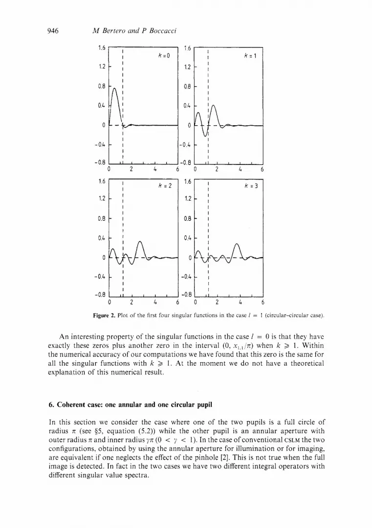
Figure 2. Plot of the first four singular functions in the case I = 1 (circular-circular case).

An interesting property of the singular functions in the case I = 0 is that they have exactly these zeros plus another zero in the interval (0, X , , , / T C ) when k 3 1. Within the numerical accuracy of our computations we have found that this zero is the same for all the singular functions with k 3 1. At the moment we d o not have a theoretical explanation of this numerical result.

6. Coherent case: one annular and one circular pupil

In this section we consider the case where one of the two pupils is a full circle of radius n (see 55, equation (5.2)) while the other pupil is an annular aperture with outer radius n and inner radius yn (0 < y < 1). In the case of conventional CSLM the two configurations, obtained by using the annular aperture for illumination or for imaging, are equivalent if one neglects the effect of the pinhole [2]. This is not true when the full image is detected. In fact in the two cases we have two different integral operators with different singular value spectra.


1 , j , , I , 1 1 , I , , , , -0.8 - 0.8

1.6

1.2

0.8

0.4

0

- 0.4

-0.8

0 2 4 6 0 2 4 6

1.6 k - 2 I

I 1 1.2

0.8

k = 3 I I I I I I I I I I I

+c&

1-0.4

U I I I I -0.e , I 1 I I ,

0 2 4 6 0 2 4

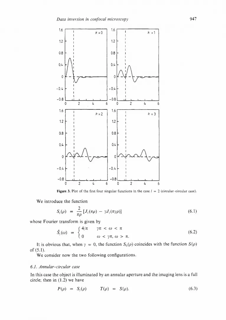
Figure 3. Plot of the first four singular functions in the case I = 2 (circular--circular case).

We introduce the function 2

=P Sy(P) = - [ J , ( Z P ) - yJ,(nyp)l

whose Fourier transform is given by y n < o < n

0 < y71,o > 71. Sl,(w) =

It is obvious that, when y = 0, the function S,(p) coincides with the function S ( p )

We consider now the two following configurations. of (5.1).

6.1. Annular-circular case

In this case the object is illuminated by an annular aperture and the imaging lens is a full circle; then in (1.2) we have

P(P) = S?(P) T(P) = S(P). (6.3)


Table 3. Singular values of the annular-circular case, with y = 0.5, for I = 0, 1, 2, 3 ( N = 240, M = 60).

k I = O I = I 1 = 2 1 = 3

0 I 2 3 4 5 6 7 8 9

I O

0.61 11 0.2312 0. IO08 0.5933 x I O - ' 0.3147 x lo- ' 0.2060 x I O - ' 0.1891 x I O - ' 0.1607 x 1 0 ~ - ' 0.1327 x I O - ' 0.9896 x 0.8846 x

0.3135 0.2017 0.8107 0.3300 x lo-' 0.2779 x IO-- ' 0.2042 x I O - ' 0.1902 x lo-' 0.1474 x lo- ' 0.1017 x I O - ' 0.9377 x 0.8792 x

0.2356 0.2093 0.1088 x I O - ' 0.8256 x I O - ' 0.6243 x I O - ' 0.3366 x lo - ' 0.3149 x I O - ' 0.2941 x lo- ' 0.2062 x IO- ' 0.2042 x lo- ' 0.1892 x I O - ' 0.1903 x I O - ' 0.1631 x lo- ' 0.1475 x I O - ' 0.1341 x I O - ' 0.1021 x 10-1 0.9899 x 0.9452 x 0.8847 x 0.8794 x 0.7711 x 0.7071 x

Using again (5.3)-(5.5) we get

Since the kernel (6.4) has the same bandwidths as the kernel (5.6), the matrix A!:!! corresponding to the kernel (6.4) can be easily obtained from (5.7), just by replacing S(+X, , ) with Sl,(+xi,wl). The result is

As in 95, approximations of the singular values of the integral operator can be obtained using a finite number of values of the indices. The convergence of the approximation is similar to that discussed in $5.

In table 3 we give the singular values x / ~ ~ , for I = 0, 1 ,2 , 3, in the case y = 0.5. These singular values have been computed in the case N = 240 and M = 60 (see 45).

In table 4 we give the behaviour of the singular values as a function of y in the case 1 = 0. The singular value xo,o is a decreasing function of y and this result is related to the fact that the light transmitted by an annular pupil decreases as the radius of the inner circle increases.

Table 4. Singular values of the annular-circular case, 1 = 0, as a function of y = 0.3, 0.5, 0.7, 0.9 (A' = 240, M = 60). ~~

k -

0 1 2 3 4 5 6 7 8 9

I O

~~

7 = 0.3 7 = 0.5 y = 0.7

0.7738 0.2113 0.1008 0.4147 x IO- ' 0.3408 x I O - ' 0.2483 x I O - ' 0.1842 x I O - ' 0.1392 x lo- ' 0.1269 x I O - ' 0.9960 x 0.8678 x

0.61 11 0.2312 0.1008 0.5933 x I O - ' 0.3147 x I O - ' 0.2060 x I O - ' 0.1891 x lo - ' 0.1607 x I O - ' 0,1327 x I O - ' 0.9896 x 0.8846 x IO-'

0.3925 0.1828 0.1130 0.6966 x lo-' 0.4428 x I O - ' 0.2964 x I O - ' 0.1578 x lo - ' 0.1491 x IO-' 0.1264 x lo- ' 0.1091 x I O - ' 0.8976 x IO-*

7 = 0.9

0.1369 0.6910 x I O - ' 0.5128 x I O - ' 0.4167 x lo- ' 0.3516 x lo-' 0.3022 x I O - ' 0.2618 x I O - ' 0.2274 x lo- ' 0.1970 x I O - ' 0.1699 x I O - ' 0.1454 x lo- '

Data inversion in confocal microscopy

-0.8

949

I I I I I I I I -0.8 , I , I I I

1.6

1.2

0.8

0.4

0

-0.4

k = 2 I I I I I I

- I I

-

- I I

1.6 k : I

I I

I I

I I

1.2 - I

0.8 - I

I

I I

-0.4 - I

-0.8 I l l I I I

0 2 4

1.2 r I

I 0.8 1 I

-0.4

Table 5. The ratios c ( ~ , ~ / c ( ~ , ~ corresponding to the singular values of table 4

k 'J = 0.3 y = 0.5 y = 0.7 y = 0.9

0 1 2 3 4 5 6 7 8 9

10

1.000 3.665 7.679 1.866 x 10 2.270 x I O 3.116 x LO 4.201 x 10 5.559 x 10 6.099 x I O 7.768 x 10 8.917 x 10

1.000 2.643 6.062 1.030 x 10 1.942 x 10 2.966 x I O 3,231 x 10 3.803 x 10 4.605 x I O 6.175 x I O 6.908 x 10

1.000 2.147 3.473 5.635 8.865 1.325 x 10 2.488 x 10 2.633 x 10 3.105 x 10 3.596 x 10 4.373 x I O

1.000 1.98 1 2.669 3.285 3.893 4.530 5.228 6.021 6.947 8.057 9.417

950

I

I I I I

- 1 I I

- 1

I k = O -

- I I

- 1 I I

, I , I , I

M Bertero and P Boccacci

1.6

1.6

1.2

0.8

0.4

0

-0.4

- 0.8

I I k = 3

1 .6

1.2

0.8

0.4

0

-0.4

-0.8

I

I I I I

- I I I

I k - 2

I - 1

I I

I I I 1 1 1

1.6

1.2

0.8

0.4

0

- 0.4

- 0.8

1.2 1 1 I

0.8 1 I I

I

1-0.8 -0.4 0 i 2 4

Figure 5. Plot of the first four singular functions in the case = 0.9 and I = 0 (annular-circular case)

In table 5 we give the ratios C ( ~ , ~ / C ( ~ , ~ for the same values of y . In this way it clearly appears that, if we consider a truncated singular function expansion, with a fixed number of terms, then the ill conditioning of this approximate solution is a decreasing function of y . The maximum of the ill conditioning is obtained in the case y = 0, i.e. in the case of circular pupils considered in $ 5 . This result can imply that i t may be useful to illuminate the object by means of an annular aperture in order to enhance the resolution. In fact the illumination profile associated with an annular aperture is narrower than that associated with a circular aperture.

In figures 4 and 5 we plot the first four singular functions for y = 0.5 and y = 0.9, in the case 1 = 0. If we compare these singular functions with those plotted in figure 1 we find that, except the case k = 0, they have two zeros inside the Rayleigh interval while the singular functions of the circular case have at most one zero.

6.2. Circular-annular case

In this configuration the illuminating pupils is a full circle while the imaging pupil is an annular aperture, so that in (1.2) we have

P(P> = S(P) U P ) = S?(P>. (6.6)

Dura inversion in confocal microscopy 95 1

Table 6. Singular values of the circular-annular case, with y = 0.5, for 1 = 0, 1, 2, 3 ( N = 240, A4 = 60).

k I = O I = 1 1 = 2

0 0.7051 1 0.1111 2 0.3742 x lo - ' 3 0.1975 x lo - ' 4 0.1245 x I O - ' 5 0.8878 x IO-* 6 0.6590 x lo-* 7 0.5187 x lo -* 8 0.4213 x IO-' 9 0.3511 x IO-'

10 0.2982 x

0.4546 0.8519 x lo- ' 0.3358 x lo- ' 0.1848 x IO- ' 0.1194 x lo- ' 0.8505 x 0.6434 x 0.5086 x IO-' 0.4146 x IO-' 0.3465 x 0.2948 x IO-'

0.2258 0.7126 x lo - ' 0.3208 x lo- ' 0.1824 x lo-- ' 0.1192 x IO- ' 0.8522 x IO-' 0.6460 x 0.5109 x 0.4166 x 10-~2 0.3479 x IO-' 0.2961 x

1 = 3

0.1323 0.5508 x I O - ' 0.2826 x lo- ' 0.1695 x I O - ' 0.1137 x I O - ' 0.8236 x 0.6296 x lo-* 0.5005 x I O - * 0.4098 x IO- ' 0.3432 x lo-' 0.2928 x

Then, the integral representation (5.3) implies that

S?(P) = 2 jo' t[Jo(npr) - y2Jd7cypr)l dt

and, from the addition theorem (5.4), we have

T,(p, p ' ) = 4n t [J/(zpt)J,(np'r) - +y2JI(ny~t)JI(nyp't)] dr (6.8)

the function T,(p, p') being defined by (3.6) and (3.7). Finally, from (3.9), (4.20) and (4.6), after some elementary computation, we get

lo'

where xi. In

XLrl BLii, = J/ + 1 1 J/ (3 x/,??, 1 - Y J , + I (YX/ .n 1 J/ ( 3 +yx,.m + 3? - J/ + I (3 1/x/.,n 14 ( " l / , t l ) .

(6.10)

We present the numerical results in the same form used for the annular-circular case. Therefore, in table 6 we give the singular values as a function of I for y = 0.5;

Table 7. Singular values of the circular-annular case, 1 = 0, as a function of y = 0.3, 0.5, 0.7, 0.9 ( N = 280, M = 280).

k p = 0.3 y = 0.5 = 0.7 p = 0.9

0 0.8109 1 0.1550 2 0.5914 x I O - ' 3 0.3193 x lo- ' 4 0.2040 x I O - ' 5 0.1443 x I O - ' 6 0.1087 x I O - ' 7 0.8571 x lo-* 8 0.6975 x lo-* 9 0.5820 x lo-*

10 0.4950 x IO-'

0.7052 0.1111 0.3744 x I O - ' 0.1976 x lo- ' 0,1246 x I O - ' 0.8784 x lo-* 0.6596 x IO- ' 0.5193 x I O - * 0.4220 x IO-* 0.3519 x 0.2991 x lo-'

0.5486 0.3117 0.6204 x I O - ' 0.1533 x I O - ' 0.1783 x lo-' 0.3436 x 0.9311 x I O - * 0.1795 x lo-* 0.5815 x IO-' 0.1108 x 0.4094 x lo-* 0.7811 x 0.3066 x I O - * 0.5830 x 0.2413 x I O - * 0.4589 x 0.1959 x lo-* 0.3717 x lo-' 0.1634 x 0.3097 x IO-' 0.1388 x lo-' 0.2624 x

952

I

I I I I

- I I I

- 1

I k = 2 -

M Bertero and P Boccacci

I

I I I I

- I I I

- 1 I

I ‘k 3 -

Table 8. The ratios xO,O/aO,k corresponding to the singular values of table 7

I - 1

I I

I l l 1 I I

k 7 = 0.3 y = 0.5

0 1.000 1 5.231 2 1.371 x 10 3 2.539 x 10 4 3.975 x 10 5 5.618 x 10 6 7.456 x 10 I 9.460 x 10 8 1.162 x 10” 9 1.393 x IO+*

10 1.638 x 10”

1.000 6.347 1.883 x 10 3.569 x 10 5.658 x 10 8.027 x 10 1.069 x lo+’ 1.358 x 1.671 x IO+’ 2.004 x IO+* 2.357 x l o + *

7 = 0.7

1.000 8.843 3.076 x 10 5.892 x 10 9.435 x 10 1.340 x 1.789 x IO+’ 2.273 x 10” 2.800 x 3.358 x I O + * 3.953 x l o k 2

y = 0.9

1.000 2.033 x 10 9.072 x 10 1.737 x 2.813 x IO+’ 3.991 x I O + * 5.348 x 10” 6.793 x IO-’ 8.388 x 1.007 10+3 1.188 x lo+’

1.6

1.2

0.8

0.4

0

-0.4

-0.8

1.6

1.2

0.8

0.4

0

-0.4

-0.8

1.6

1.2

0.8

0.4

0

-0.4

-0.8

I

I I I I

‘ I

I k = l

! I , 1 I I

2 4

0 2 4 6 0 2 4 6

Figure 6. Plot of the first four singular functions in the case y = 0.5 and I = 0 (circular-annular case).


in table 7 we give the singular values as a function of y for I = 0 and in table 8 we give the ratios cqO/cqk corresponding to the singular values of table 7.

We point out that the convergence of the singular values, for increasing values of N amd M, is slower in this case than in the cases previously considered. This is especially true when y tends to 1.

When y = 0.9, using the maximum number of points allowed by our program, i.e. N = M = 280, we still have an error on the second digit of the last singular values given in table 7. On the other hand, in the case y = 0.5, a comparison between table 6 and table 7 shows that with N = 240, M = 60 the first three digits are correct for almost all the first eleven singular values.

If we compare table 8 with table 5 we notice that the ill conditioning of the truncated singular function expansions in the circular-annular configuration is greater than the ill conditioning of the same solutions in the annular-circular case (and also greater than the ill conditioning of the circular-circular case). Moreover, for fixed k , the ill conditioning is an increasing function of y . Therefore the use of an annular aperture as imaging system does not seem to be convenient for obtaining the super-resolving effect. Further investi- gations, however, are required to confirm this conclusion.

Finally in figure 6 we plot the first four singular functions for y = 0.5, in the case I = 0. We notice that, except in the case k = 2, the singular functions with k > 0 have only one zero inside the Rayleigh interval.

7. Coherent case: annular pupils

In this section we consider the case where both pupils are annular apertures. Moreover we assume, for simplicity, that they have the same inner and outer radius, given respectively by yn and (0 < y < 1). Then we have

the function S?((p) being defined in (6.1).

Table 9. Singular values of the annular-annular case, with y = 0.5, for 1 = 0, 1, 2, 3 ( N = 240, A4 = 60).

k l = O I = 1 1 = 2 1 = 3

0 1 2 3 4 5 6 7 8 9

10

0.5186 0.2956 0.2201 0.2060 0.9408 x I O - ' 0.1390 0.9065 x I O - ' 0.6753 x I O - ' 0.5613 x I O - ' 0.3235 x I O - ' 0.4031 x I O - ' 0.3055 x lo - ' 0.1872 x I O - ' 0.2717 x I O - ' 0.1797 x I O - ' 0.2144 x I O - ' 0.1681 x lo - ' 0.1252 x I O - ' 0.1582 x lo - ' 0.1230 x I O - ' 0.9861 x lo-* 0.1108 x lo- ' 0.9566 x IO- ' 0.1031 x I O - ' 0.7612 x IO-' 0.7498 x 0.7511 x I O - * 0.7314 x IO-* 0.6291 x 0.5879 x I O - * 0.6182 x I O - * 0.5778 x IO-* 0.4536 x IO-* 0.5116 x 0.4519 x IO-' 0.5018 x IO-' 0.4446 x IO-' 0.3770 x 0,4384 x IO-' 0.3773 x IO-' 0.3347 x IO-' 0.3758 x IO- ' 0.3326 x 0.3678 x


Table 10. Singular values of the annular-annular case, I = 0. as a function of 7 = 0.3. 0.5, 0.7, 0.9 ( N = 280, M = 280).

k ,I - y = 0.3 , - 0.5

0 1 2 3 4 5 6 7 8 9

10

0.7240 0.1473 0.8471 x lo - ' 0.2814 x lo-' 0.2718 x lo- ' 0.1463 x lo - ' 0.1220 x 10-1 0.9249 x lo-* 0.7240 x 0.6474 x 0.5155 x lo-*

0.5187 0.9412 x lo - ' 0.5617 x I O - ' 0.1873 x lo- ' 0.1682 x I O - ' 0.9871 x lo-* 0.7617 x lo-' 0.6302 x lo-' 0.4539 x 0.4461 x lo-' 0.3369 x lo-*

~- ~~

y = 0.7

0.2840 0.4618 x 10.' 0.2816 x lo - ' 0.9319 x IO- ' 0.8120 x lo-' 0.4909 x IO- ' 0.3677 x I O - * 0.3133 x lo--* 0.2218 x 0,1493 x 0.1675 x

7 = 0.9

0.6670 x l o - ' 0.9291 x lo-' 0.5742 x lo-' 0.1881 x 0.1622 x 0.9883 x lo-' 0.7344 x lo-' 0.6293 x l o - ' 0.4451 x IO- ' 0.4364 x lo- ' 0.3326 x I O - '

From the results of the previous section it follows that the matrix A$; is given by

with B i i given by (6.10). In table 9 we give the singular values for I = 0, 1,2, 3 in the case y = 0.5. These have

been obtained with N = 240, M = 60. The convergence of the approximation is similar to that obtained in the circular-annular case. For this reason in tables 10 and 11 we give the results obtained using the maximum number of points allowed by our program, i.e. N = M = 280.

In Table 10 we give the singular values in the case I = 0 for various values of y . Also in this case we notice that the singular values are decreasing functions of y . In fact they tend to zero when y + 1 and this is again a consequence of the fact that, when y -+ 1, the intensity of the light transmitted by the two apertures tend to zero. Therefore the interesting quantities are again the ratios ~ 1 ~ , ~ / a , , , . These are given in table 11 and we find that these ratios are increasing functions of y , i.e. the ill conditioning of the truncated singular function expansions increases for increasing values of y. Again, such a result is analogous to that obtained in the circular-annular case.

Table 11. The ratios ~ ( ~ , ~ j c i ~ , ~ corresponding to the singular values of table I O

k y = 0.3 7 = 0.5 y = 0.7 >' = 0.9

0 1.000 1,000 1.000 1.000 1 4.915 5.51 1 6.151 7.178 2 8.547 9.235 1.009 x I O 1.161 x 10 3 2.573 x 10 2.769 x I O 3.048 x 10 3.547 x 10 4 2.664 x 10 3.084 x !O 3.500 x 10 4.111 x 10 5 4.949 x 10 5.255 x 10 5.786 x 10 6.748 x I O 6 5.935 x 10 6.810 x 10 7.724 x 10 9.081 x I O 7 7.828 x I O 8.231 x 10 9.066 x 10 1.060 x lo** 8 1.000 x 1.143 x 1.280 x lo+' 1.499 x lo+' 9 1.118 x lo+' 1.163 x 1.296 x lo+* 1.528 x

I O 1.405 x 10" 1.540 x 1.696 x lo+' 2.005 x I O + '

Data inversion in confocal microscopy

1.6

1.2

0.8

0.4

955

I

- I

k = 3 I I

I I

- I I I

I - I

1.6

1.2

0.8

0.4

0

-0.4

-0.8

k = 2 I I I I I I I I I I I I

I _ - I I

- I 1 I

I I I I I I

~~

1.6

1.2

0.8

0.4

0

- 0.4

- 0.8

-0.4

-0.8

I

I I

- I

, I , I I I

Figure 7. Plot of the first four singular functions in the case y = 0.5 and I = 0 (annular-annular case)

In figure 7 we plot the first four singular functions in the case y = 0.5. We notice that the singular functions with k = 2 , 3 have two zeros inside the Rayleigh interval.

8. Concluding remarks

In this paper we have proposed a numerical method for the computation of the singular system of the integral operators related to the problem of data inversion in super- resolving CSLM. The method applies to the case where the optical system has circular symmetry and it has been tested for several configurations of the illuminating and imaging lenses, assuming aberration-free objectives.

The interesting result is that the ill conditioning of the truncated singular function expansion of the solution depends on the configuration. We summarise the results in table 12 where we compare the condition numbers of the circular-circular case (cc) with the condition numbers of the annular-circular (AC), circular-annular (CA) and annular-annular (AA), all the annular apertures being characterised by 7 = 0.5 (see (6.1)).


Table 12. Comparison of the condition numbers for the configuration considered in this paper: (AC) = annular-circular; (cc) = circular-circular; (AA) = annular-annular; (CA) = circular-annular, All the annular apertures are characterised by y = 0.5.

0 1.000 1.000 1.000 1.000 1 2.643 4.607 5.511 6.347

.2 6.062 1.070 x 10 9.235 1.883 x 10 3 1.030 x 10 1.876 x 10 2.769 x 10 3.569 x 10 4 1.942 x 10 2.833 x 10 3.084 x 10 5.658 x 10 5 2.966 x 10 3.919 x I O 5.255 x 10 8.027 x I O

These results can have a rather simple physical interpretation. In fact an annular aperture provides an illuminating profile which is narrower than the profile of a circular aperture; on the other hand an annular aperture, when used as an imaging system, transmits less information than a circular one. If we look at the results of table 12 we find that the smallest ill conditioning corresponds to the configuration (AC) and the largest one to the configuration (CA). The configurations (cc) and (AA) are intermediate. In fact (cc) is best for the imaging but not for the illumination. On the other hand (AA) is best for the illumination but not for the imaging. In conclusion these results seem to indicate that the use of an annular aperture for the illuminating system can facilitate the super-resolving effect in CSLM. The investigation of the transfer functions will be the subject of a future publication and it is important in order to confirm the previous conclusion. This point, however, is out of the scope of this paper, which is mainly devoted to the presentation of the numerical method.

Acknowledgments

This work has been partly supported by EEC Contract No. BAP-0293-NL(GDF) and by MPI, Italy.

References

Lemons R A and Quate C F 1974 Acoustic microscopy-scanning v-sion Appl. Phys. Lett. 24 163-5 Sheppard C J R and Choudhury A 1977 Image formation in the scanning microscope Opt. Acta 24

105 1-73 Brakenhoff G J, Blom P and Barends P 1979 Confocal scanning light microscopy with high aperture

immersion lenses J . Microsc. 117 219-32 Bertero M and Pike E R 1982 Resolution in diffraction limited imaging, a singular value analysis, I. The

case of coherent illumination Opt. Acta 29 727-46 Bertero M, De Mol C, Pike E R a n d Walker J G 1984 Resolution in diffraction limited imaging, a singular

value analysis. IV. The case of uncertain localization or non-uniform illumination Opt. Acta 31

Bertero M, Brianzi P and Pike E R 1987 Super-resolution in confocal scanning microscopy Inverse Problems 3 195-2 12

Bertero M, Boccacci P, Brianzi P and Pike E R 1987 Inverse problems in confocal scanning microscopy Inverse Problems: An Interdisciplinary Study ed P C Sabatier Adv. Electr. and Electron. Phys. (Suppl.)

923-46

19 225-239


[8] Bertero M, De Mol C and Pike E R 1987 Analytic inversion formula for confocal scanning microscopy

[9] Bertero M, Boccacci P and Pike E R 1988 Inverse problems in fluorescence confocal scanning microscopy

[IO] Bertero M, Boccacci P, Defrise M, De Mol C and Pike E R 1988 Super-resolution in confocal scanning

[ l l ] Groetsch C W 1977 Generalized Inverses of Linear Operators (New York: Dekker) [I21 Papoulis A 1968 Systems and Transform with Applications to Optics (New York: McGraw-Hill) [I31 Watson G N 1952 A Treatise on lhe Theory qf Bessel Functions (Cambridge: Cambridge University Press) [14] Bertero M , De Mol C and Pike E R 1985 Linear inverse problems with discrete data. I: General

J . Opt. Soc. Am. A 4 1748-50

SPIE Proc. Vol 1028

microscopy: 11. The incoherent case Inverse Problems 5 441-61

formulation and singular system analysis Inverse Problems 1 301-30

Documents

Computation of the singular system for a class of integral operators related to data inversion in confocal microscopy