Embed Size (px)
Citation preview

arX
iv:m
ath/
0403
016v
2 [
mat
h.PR
] 1
3 D
ec 2
004
CONDITIONAL MOMENTS OF q-MEIXNER PROCESSES
W LODZIMIERZ BRYC AND JACEK WESO LOWSKI
Abstract. We show that stochastic processes with linear conditional expec-tations and quadratic conditional variances are Markov, and their transitionprobabilities are related to a three-parameter family of orthogonal polynomi-als which generalize the Meixner polynomials. Special cases of these processesare known to arise from the non-commutative generalizations of the Levy pro-cesses.
1. Introduction
1.1. Motivation. It has been known since the work of Biane [10] that every non-commutative process with free increments gives rise to a classical Markov process,whose transition probabilities ”realize” the non-commutative free convolution ofthe corresponding measures. It is natural to ask how to recognize in classical prob-abilistic terms which Markov processes might arise from this construction. Unfor-tunately, the non-commutative freeness seems to be poorly reflected in the corre-sponding classical Markov process, which makes it hard to answer this question. Amore general framework might be less constraining and easier to handle.
Non-commutative processes with free increments can be thought as a specialcase corresponding to the value q = 0 of the more general class of q-Levy processes[3], [6]. Markov processes are known to arise in this more general setting in twoimportant cases: Bozejko, Kummerer, and Speicher, give explicit Markov transitionprobabilities for the q-Brownian motion, see [12, Theorem 1.10], and Anshelevich[7, Corollary A.1] proves the corresponding result for the q-Poisson process. Otherq-Levy processes are still not well understood, so it is not known whether Markovprocesses arise in the general case; for indications that Markov property may per-haps fail, see [5].
This paper arose as an attempt to better understand the emergence of relatedMarkov processes from probabilistic assumptions. We define our class of processesby assuming that the first two conditional moments are given respectively by thegeneric linear and quadratic expressions. Such assumptions are familiar from Levy’scharacterization of the Wiener process as a martingale and a quadratic martin-gale with continuous trajectories. For more general processes the assumption ofcontinuity of trajectories fails, so we replace it by conditioning with respect notonly to the past, but also to the future. This approach originated with Plucinska
Date: February 17, 2004. Revised: May 12, 2004. Corrected: November 18, 2004.2000 Mathematics Subject Classification. 60J25.Key words and phrases. Quadratic conditional variances, harnesses, polynomial martingales,
hypergeometric orthogonal polynomials, free Levy processes, classical versions of non-commutativeprocesses, q-Meixner processes .
Research partially supported by NSF grant #INT-0332062, by the C.P. Taft Memorial Fund,and University of Cincinnati’s Summer Faculty Research Fellowship Program.
1

2 W LODZIMIERZ BRYC AND JACEK WESO LOWSKI
[24] who proved that processes with linear conditional expectations and constantconditional variances are Gaussian. Subsequent papers covered discrete Gaussiansequences [17], L2-differentiable processes [29], Poisson process [15], Gamma pro-cess [32]. Weso lowski [33] unified several partial results, identifying the generalquadratic conditional variance problem which characterizes the five Levy processesof interest in this note: Wiener, Poisson, Pascal, Gamma, and Meixner. Our mainresult, Theorem 3.5, extends [33, Theorem 2] to the more general quadratic condi-tional variances. Similar analysis of stationary sequences in [16] yields the classicalversions of the non-commutative q-Gaussian processes of [12]. Further contributionsto the stationary case can be found in [22].
Stochastic processes with linear conditional expectations and quadratic condi-tional variances turn out to depend on three numerical parameters −∞ < θ <∞, τ ≥ 0, and −1 ≤ q ≤ 1. They are Markov, and arise from the non-commutativeconstructions, at least for those values of the parameters when such constructionsare known. To point out the connection with the orthogonal polynomials fromwhich they are derived, we call them q-Meixner processes.
When q = 1, the q-Meixner processes have independent increments and we re-cover the five Levy processes from [33, Theorem 2]. For other values of parameterq, we encounter several processes that arose in non-commutative probability. Ifτ = θ = 0, we get the classical version of the q-Brownian motion [12]. If τ = 0, θ 6= 0the q-Meixner processes arise as the classical version from the q-Poisson process de-fined in [3, Def. 6.16]. When q = 0 the q-Meixner processes are related to theclass of free Levy processes considered by Anshelevich [4].
The reasons why these special cases of q-Meixner processes should arise from theFock space constructions are not clear to us. It is not known whether the genericq-Meixner process arises as a classical version of a non-commutative process, butthe situation must be more complex. The connection with the q-Levy processeson the q-Fock space as defined in [3] fails for the following reason. In Proposition3.3 below we establish a polynomial martingale property (46) for all q-Meixnerprocesses. But from Anshelevich [5, Appendix A.2] we know that a generic q-Levyprocess does not have martingale polynomials; the exceptions are q = 0, q = 1, theq-Poisson process, and the q-Brownian motion, and these are precisely the casesthat we already mentioned above.
1.2. Assumptions. Throughout this paper (Xt)t≥0 is a separable square-integrablestochastic process, normalized so that for all t, s ≥ 0
(1) E(Xt) = 0, E(XtXs) = min{t, s}.We are interested in the processes with linear conditional expectations and qua-dratic conditional variances. More specifically, we assume the following.
For all 0 ≤ s < t < u,
(2) E(Xt|F≤s ∨ F≥u) = aXs + bXu,
where a = a(s, t, u), b = b(s, t, u) are the deterministic functions of s, t, u, andF≤s ∨ F≥u denotes the σ-field generated by {Xt : t ∈ [0, s] ∪ [u,∞)}.
For ease of reference, we list the following trivial consequences of (2). From theform of the covariance it follows that
(3) a =u − t
u − s, b =
t − s
u − s.

q-MEIXNER PROCESSES 3
Notice that from (2) we have
E(E(Xt|Fs) − Xs)2 = E(E(E(Xt|F≤s ∨ F≥u)|Fs) − Xs)2
= b2E(E(Xu − Xs|Fs))2 ≤ (t − s)2/(u − s).
Passing to the limit as u → ∞ we see that
(4) E(Xt|F≤s) = Xs
for 0 ≤ s ≤ t. Similarly, taking s = 0 in (2) we get
(5) E(Xt|F≥u) =t
uXu.
Processes which satisfy condition (2) are sometimes called harnesses, see [21], [34].We assume in addition that the conditional variance of Xt given F≤s∨F≥u is givenby a quadratic expression in Xs, Xu. Recall that the conditional variance of Xwith respect to a σ-field F is defined as
Var(X |F) = E(X2|F) − (E(X |F))2.
For later calculations, it is convenient to express this assumption as follows.For all 0 ≤ s < t < u,
E(X2t |F≤s ∨ F≥u) = AX2
s + BXsXu + CX2u + D + αXs + βXu,(6)
where A = A(s, t, u), B = B(s, t, u), C = C(s, t, u), D = (s, t, u), α = α(s, t, u), β =β(s, t, u) are the deterministic functions of s, t, u.
Since X0 = 0, the coefficients a, A, B, α are undefined at s = 0. In some formulasfor definiteness we assign these values by continuity.
It turns out that under mild assumptions, the functions A, B, C, D, α, β, aredetermined uniquely as explicit functions of s, t, u, up to some numerical con-stants. The next assumption specifies two of these constants by requesting thatVar(Xt|F≤s) = const for all 0 ≤ s ≤ t. We use (4) to state this assumption in thefollowing more explicit form.
(7) E(X2t |F≤s) = X2
s + t − s.
Notice that equations (4) and (7) imply that {Xt : t ≥ 0} and {X2t − t : t ≥ 0}
are martingales with respect to the natural filtration F≤t; these two martingaleconditions (and continuity of trajectories) are the usual assumptions in the Levytheorem.
2. Conditional variances
It is interesting to note that under mild assumptions, assumption (6) can be writ-ten explicitly, up to some numerical constants. Two of these numerical constantsappear already under one-sided conditioning.
Proposition 2.1. Let (Xt)t≥0 be a separable square integrable stochastic processwhich satisfies conditions (1), (2), and such that 1, Xt, X
2t are linearly independent
for all t > 0. If for every 0 < t < u the conditional expectation E(X2t |F≥u) is a

4 W LODZIMIERZ BRYC AND JACEK WESO LOWSKI
quadratic expression in variable Xu, then there are constants τ ∈ [0,∞] and θ ∈ R
such that
(8) Var(Xt|F≥u) =
t(u−t)u+τ
(
τX2
u
u2 + θ Xu
u + 1)
if τ < ∞,
t(u − t)(
X2u
u2 + θ Xu
u
)
if τ = ∞.
for all 0 ≤ t < u.
Proof. By assumption, for any 0 < s < t
(9) E(X2s |F≥t) = m(s, t)X2
t + n(s, t)Xt + o(s, t) ,
where m, n, o are some functions.On the other hand from (5) we get
E(XsXt|F≥u) = E(E(Xs|F≥t)Xt|F≥u) =s
tE(X2
t |F≥u),
and from (2) we get
E(XsXt|F≥u) = E(XsE(Xt|F≤s ∨ F≥u)|F≥u)
=u − t
u − sE(X2
s |F≥u) +t − s
u − sXuE(Xs|F≥u)
=u − t
u − sE(X2
s |F≥u) +(t − s)s
(u − s)uX2
u .
Combining the above two formulas we have
(10)s
tE(X2
t |F≥u) =u − t
u − sE(X2
s |F≥u) +(t − s)s
(u − s)uX2
u.
Now we substitute the conditional moments from (9) into (10), gettings
t
(
m(t, u)X2u + n(t, u)Xu + o(t, u)
)
=u − t
u − s
(
m(s, u)X2u + n(s, u)Xu + o(s, u)
)
+(t − s)s
(u − s)uX2
u .
Recall that 1, Xu, X2u are linearly independent. Comparing the coefficients of re-
spective powers of Xu we obtain
s
tm(t, u) =
u − t
u − sm(s, u) +
(t − s)s
(u − s)u,
s
tn(t, u) =
u − t
u − sn(s, u) ,
s
to(t, u) =
u − t
u − so(s, u) .
The first equation leads to(
m(t, u)
t− 1
u
)
1
u − t=
(
m(s, u)
s− 1
u
)
1
u − s,
and hence
m(t, u) =t
u+ t(u − t)i(u)
for some function i : R → R. The next two equations give
n(t, u) = t(u − t)j(u) and o(t, u) = t(u − t)k(u)
for some functions j, k : R → R. Thus from (9) we get
E(X2t |F≥u) =
(
t
u+ t(u − t)i(u)
)
X2u + t(u − t)j(u)Xu + t(u − t)k(u) .

q-MEIXNER PROCESSES 5
Taking the expectations of both sides we get t = t + tu(u− t)i(u) + t(u− t)k(u), sok(u) = −ui(u). Finally we have
(11) E(X2t |F≥u) =
t
uX2
u + t(u − t)[
i(u)(X2u − u) + j(u)Xu
]
.
To identify the functions i and j we fix s < t < u and insert (11) into the formula
E(X2s |F≥u) = E(E(X2
s |F≥t)|F≥u) .
This givess
uX2
u + s(u − s)[
i(u)(X2u − u) + j(u)Xu
]
= E( s
tX2
t + s(t − s)[
i(t)(X2t − t) + j(t)Xt
]
∣
∣
∣F≥u
)
=s
t
{
t
uX2
u + t(u − t)[
i(u)(X2u − u) + j(u)Xu
]
}
+s(t − s)i(t)
{
t
uX2
u + t(u − t)[
i(u)(X2u − u) + j(u)Xu
]
}
+s(t − s)j(t)t
uXu − st(t − s)i(t) .
Comparing the coefficients of respective powers of Xu we obtain
(12) ui(u) = ti(t) + (u − t)ti(t)ui(u) ,
(13) uj(u) = tj(t) + (u − t)ti(t)uj(u) .
If i is non-zero for all t > 0 then (12) gives 1ti(t) + t = 1
ui(u) + u. This means that1
ti(t) + t = −τ for some constant τ , and τ ≥ 0 since 1/i(t) cannot vanish for any
t > 0. Hence
(14) i(t) = − 1
t(t + τ).
Using this in (13) we get u(u + τ)j(u) = t(t + τ)j(t). Thus
j(t) =θ
t(t + τ)
for some real constant θ. We get
(15) E(X2s |F≥t) =
s(s + τ)
t(t + τ)X2
t +s(t − s)
t(t + τ)θXt +
s(t − s)
t + τ.
Suppose now that i(t) = 0 for some t > 0. Then (12) implies that i is a zerofunction, corresponding to τ = ∞ in (14). In this case (13) leads to uj(u) = tj(t),which means that j(t) = θ/t for some real number θ. Thus in this case
(16) E(X2s |F≥t) =
s
tX2
t +s(t − s)
tθXt .
�
Notice that taking the expected value of both sides of (6), we get a trivial relation
(17) t − As − Cu = Bs + D,
valid for all 0 ≤ s < t < u. We need additional relations between the coefficients in(6).

6 W LODZIMIERZ BRYC AND JACEK WESO LOWSKI
Lemma 2.2. Let (Xt)t≥0 be a separable square integrable stochastic process whichsatisfies conditions (1), (2), and such that 1, Xt, X
2t are linearly independent for all
t > 0. Suppose that condition (6) holds with D(s, t, u) 6= 0 for all 0 ≤ s < t < u.Then the conditional expectation E(X2
u|F≤t) is quadratic in Xt for any 0 ≤ t < u.Moreover,
(18) E(X2u − u|F≤s) =
(
1 +A + B + C − 1
b − C
)
(X2s − s) +
α + β
b − CXs.
Proof. Equation (4) implies that E(X2t |F≤s) = E(XtXu|F≤s), so from (2) we get
E(X2t |F≤s) = aX2
s + bE(X2u|F≤s).
From (6) we get
E(X2t |F≤s) = AX2
s + BX2s + CE(X2
u|F≤s) + (α + β)Xs + D.
Notice that this implies C 6= b. Indeed, if C = b then subtracting the equations weget a quadratic equation for Xs. If this equation is non-trivial, then 1, Xs, X
2s are
linearly dependent. So the coefficients in the quadratic equation must all be zero;in particular, D = 0, contradicting the assumption.
Since C 6= b, we can solve the equations for E(X2t |F≤s) and E(X2
u|F≤s). Using(17), we get (18) after a calculation. �
Lemma 2.3. Let (Xt)t≥0 be a separable square integrable stochastic process whichsatisfies conditions (1), (2), (7) and such that 1, Xt, X
2t are linearly independent for
all t > 0. Suppose that condition (6) holds with D(s, t, u) 6= 0 for all 0 ≤ s < t < u.Then the conditional expectations E(X2
s |F≥t) are quadratic in Xt for any 0 ≤ s < t.Moreover, there are constants 0 ≤ τ < ∞,−∞ < θ < ∞ such that (8) holdstrue, and the parameters in (6), evaluated at 0 ≤ s < t < u, satisfy the followingequations.
A + B + C = 1,(19)
As2 + Bsu + Cu2 − t2 = τD,(20)
sα + uβ = θD,(21)
α + β = 0.(22)
Proof. Comparing the coefficients in (7) and (18), we get (19), and (22).Setting s = 0 in (6) we see that E(X2
t |F≥u) is quadratic in Xu. Thus Proposition2.1 implies that (8) holds true. Notice that since D(0, t, u) 6= 0, we must haveτ < ∞, so (15) holds. We use the latter in
E(X2t |F≥u) = AE(X2
s |F≥u) +s
uBX2
u + CX2u + (
s
uα + β)Xu + D,
which follows from (6). We get (20) from the comparison of the quadratic terms,and (21) from the comparison of the linear terms. �
For future reference we state the following.

q-MEIXNER PROCESSES 7
Remark 2.1. The system of equations (17), (19), (21), (20), (21), (22) has thesolution
α = D−θ
u − s,(23)
β = Dθ
u − s,(24)
A =ta
s− D
u + τ
s(u − s),(25)
B = Ds + u + τ
s(u − s)− u − s
sab,(26)
C = b − D1
u − s.(27)
We need the following version of [33, Theorem 2].
Proposition 2.4. Let (Xt)t≥0 be a separable square integrable stochastic processwhich satisfies conditions (1), (2), (6), and (7). Suppose that the coefficient D in(6) satisfies D(s, t, u) 6= 0 for all 0 ≤ s < t < u, and that 1, Xt, X
2t are linearly
independent for all t > 0. Then E(|Xt|p) < ∞ for all p ≥ 0.Moreover, if (Xt) and (Yt) satisfy these assumptions with the same coefficients
in (6), then the joint moments of both processes are equal,
E(Xn1
t1 Xn2
t2 . . . Xnk
tk) = E(Y n1
t1 Y n2
t2 . . . Y nk
tk)
for all t1, t2, . . . , tk > 0, n1, n2, . . . , nk ∈ N, k ∈ N.
Proof. Fix s < t and let {tk : k ≥ 0} be an arbitrary infinite strictly increasingsequence which contains s and t as consecutive elements, say s = tN , t = tN+1 forsome N ∈ N.
We apply [33, Theorem 2] to the sequence ξk = Xtk. Of course,
σ(ξ1, . . . , ξk, ξk+1) ⊂ F≤tk−1∨ F≥tk+1
. Therefore, conditions (4), (2), (7), and (6)
imply [33, (6), (7), (8), and (9)], respectively. Since corr(ξk−1 , ξk) =√
tk−1/tk 6=0,±1, the assumption [33, (10)] holds true, too. Finally, notice that Weso lowski’sαk = 1, and his ak = C(tk−1, tk, tk+1) 6= ak = b(tk−1, tk, tk+1) because from (27)we see that D 6= 0 if and only if C 6= b. Thus [33, (11)] hold true. From [33,Theorem 2] we see that E(|Xt|p) < ∞ for all p > 0, and that for n = 1, 2 . . . , theconditional moment E(Xn
t |Xt1 , . . . , XtN−1, Xs) is a unique polynomial of degree n
in the variable Xs.If two processes satisfy the assumptions, then the conditional moments of both
processes can be expressed as polynomials with the same coefficients. This impliesthat all joint moments of the processes are equal. �
Next we give the general form of the conditional variance under the two-sidedconditioning.
Proposition 2.5. Let (Xt)t≥0 be a separable square integrable stochastic processwhich satisfies conditions (1), (2), (6), and (7). Suppose that the coefficient D in(6) satisfies D(s, t, u) 6= 0 for all 0 ≤ s < t < u, and that 1, Xt, X
2t are linearly
independent for all t > 0. Then there are parameters −∞ < θ < ∞, and 0 ≤ τ < ∞such that the first part of (8) holds true. In addition, there exists −1 < q ≤ 1 such

8 W LODZIMIERZ BRYC AND JACEK WESO LOWSKI
that
Var(Xt|F≤s ∨ F≥u) =(28)
(u − t)(t − s)
u + τ − qs
(
(1 − q)(Xu − Xs)(sXu − uXs)
(u − s)2+ τ
(Xu − Xs)2
(u − s)2+ θ
Xu − Xs
u − s+ 1
)
.
Proof. By Proposition 2.4, all moments of Xt are finite. Fix s < t. Then from (5)and (7) we get s
t E(X3t ) = E(X2
t Xs) = EX3s , so E(X3
t )/t does not depend on t > 0.On the other hand, from (15) we get
E(X3s ) = E(X2
s Xt) =s(s + τ)
t(t + τ)E(X3
t ) +s(t − s)
t + τθ.
Hence
(29) EX3t = tθ.
Similarly, from (7) we get
E(X2t X2
s ) = EX4s + s(t − s),
and from (8) we get
E(X2t X2
s ) =s(s + τ)
t(t + τ)EX4
t + θs(t − s)
t(t + τ)E(X3
t ) + stt − s
t + τ.
Using (29) we get after a calculation thatE(X4
s )−s(s+θ2)s(s+τ) does not depend on s.
Thus
(30) E(X4t ) = (1 + q)t(t + τ) + t(t + θ2)
for some constant q ∈ R.A calculation gives
E(Xt − Xs)2 = t − s, E(Xt − Xs)3 = θ(t − s),
and
E(Xt − Xs)4 = (t − s)(
6s + θ2 − τ + (2 + q)(t + τ − 3s))
.
Since the determinant
1
(t − s)2det
1 E(Xt − Xs) E((Xt − Xs)2)E(Xt − Xs) E((Xt − Xs)2) E((Xt − Xs)3)
E((Xt − Xs)2) E((Xt − Xs)3) E((Xt − Xs)4)
= q (t + τ − 3s) + s + t + τ
is non-negative, taking s = t − 1 and t → ∞, we get q ≤ 1. Since 1, Xt, X2t are
linearly independent, the determinant evaluated at s = 0 must be strictly positive,see [19, pg. 19]. This shows that q > −1.
It remains to determine the coefficients in (6). Fix s < t < u. Comparing thetwo representations of E(XtX
2u|F≤s) as
E(E(Xt|F≤s ∨ F≥u)X2u|F≤s) = E(XtE(X2
u|F≤t)|F≤s),
and the similar two expressions for E(X2t Xu|F≤s), we get two different expressions
for E(X3t |F≤s). Equating them, we get
aX3s + bE(X3
u|F≤s)
= AX3s + BX3
s + BXs(u − s) + CE(X3u|F≤s) + DXs + (α + β)X2
s + β(u − s).
q-MEIXNER PROCESSES 9
We can solve this equation for E(X3u|F≤s), as (27) implies that C 6= b. Using (24)
and (19), the answer simplifies to
E(X3u|F≤s) = X3
s +B(u − s) + D
b − CXs + (u − s)
β
b − C.
From this we get
s
uE(X4
u) = E(XsX3u) = E(X4
s ) +B(u − s) + D
D(u − s)s.
Substituting (30) we deduce the following equation
(31)(u − s)B
D= 1 + q.
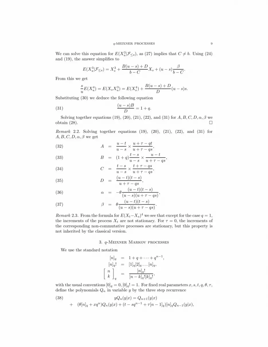
Solving together equations (19), (20), (21), (22), and (31) for A, B, C, D, α, β weobtain (28). �
Remark 2.2. Solving together equations (19), (20), (21), (22), and (31) forA, B, C, D, α, β we get
A =u − t
u − s× u + τ − qt
u + τ − qs,(32)
B = (1 + q)t − s
u − s× u − t
u + τ − qs,(33)
C =t − s
u − s× t + τ − qs
u + τ − qs,(34)
D =(u − t)(t − s)
u + τ − qs,(35)
α = −θ(u − t)(t − s)
(u − s)(u + τ − qs),(36)
β = θ(u − t)(t − s)
(u − s)(u + τ − qs).(37)
Remark 2.3. From the formula for E(Xt−Xs)4 we see that except for the case q = 1,the increments of the process Xt are not stationary. For τ = 0, the increments ofthe corresponding non-commutative processes are stationary, but this property isnot inherited by the classical version.
3. q-Meixner Markov processes
We use the standard notation
[n]q = 1 + q + · · · + qn−1,
[n]q! = [1]q[2]q . . . [n]q,[
nk
]
q
=[n]q!
[n − k]q![k]q!,
with the usual conventions [0]q = 0, [0]q! = 1. For fixed real parameters x, s, t, q, θ, τ ,define the polynomials Qn in variable y by the three step recurrence
yQn(y|x) = Qn+1(y|x)(38)
+ (θ[n]q + xqn)Qn(y|x) + (t − sqn−1 + τ [n − 1]q)[n]qQn−1(y|x),

10 W LODZIMIERZ BRYC AND JACEK WESO LOWSKI
where n ≥ 1, and Q−1(y|x) = 0, Q0(y|x) = 1, so Q1(y|x) = y − x. It is well knownthat such polynomials are orthogonal with respect to a probability measure if thelast coefficient of the three step recurrence is positive, see [19, Theorem I.4.4].Therefore, (38) defines a probability measure whenever x, θ ∈ R, 0 < s < t, τ ≥0,−1 ≤ q ≤ 1. Moreover, in this case
(39)∑
n
1√
(t − sqn−1 + τ [n − 1]q)[n]q= ∞,
so from Carleman’s criterion (see [28, page 59]), this measure is unique. We denotethis unique probability measure by µx,s,t(dy).
Of course, µx,s,t(dy) = µx,s,t,q,θ,τ(dy) depends on all the parameters of the recur-rence (38). It is worth noting explicitly that if q = −1 then [2]q = 0, so µx,s,t(dy)is supported on two points only. In general, more explicit expressions for µx,s,t(dy)can perhaps be derived from [9, Theorem 2.5] by taking their parameters b = c = 0,
ad = −(s(1 − q) + τ)/(t(1 − q) + τ), a + d = ((1 − q)x − 1)/√
t + τ/(1 − q).If we need to indicate the dependence of the polynomials in (38) on the additional
parameters in the recurrence (38), we write Qn(y|x, s, t).We will need two algebraic identities; the first one resembles [2, (2.3)] but is in
fact different; the second one is a slight generalization of [18, Theorem 1].
Lemma 3.1. For every x, y, z ∈ R, n ∈ N, and 0 ≤ s ≤ t ≤ u we have
Qn(z|x, s, u) =n∑
k=0
[
nk
]
q
Qn−k(y|x, s, t)Qk(z|y, t, u).(40)
Furthermore,
Qn(z|y, t, u)(41)
=
n∑
k=1
[
nk
]
q
Qn−k(0|y, t, 0) (Qk(z|0, 0, u) − Qk(y|0, 0, t)) .
Proof. Consider first the case |q| < 1. It is easy to check by q-differentiation withrespect to ζ that the generating function
φ(ζ, y, x, s, t) =
∞∑
n=0
ζn
[n]q!Qn(y|x, s, t)
of the polynomials Qn is given by
φ(ζ, y, x, s, t) =
∞∏
k=0
1 + θζqk − (1 − q)xζqk + ((1 − q)s + τ)ζ2q2k
1 + θζqk − (1 − q)yζqk + ((1 − q)t + τ)ζ2q2k.
For details, see [2]. Notice that for |q| < 1, the series defining φ(ζ, y, x, s, t) convergesfor all |ζ| small enough. Indeed, from (38) we get by induction |Qn+1| ≤ Cn withC = max{1, (|x| + |y| + |θ| + τ + t + s)/(1 − |q|)2}.
Therefore,
(42) φ(ζ, z, x, s, u) = φ(ζ, y, x, s, t)φ(ζ, z, y, t, u),
which implies (40) for all n ≥ 0 and |q| < 1. Since (40) is an identity between thepolynomial expressions in variables z, y, q, it must hold for all q.

q-MEIXNER PROCESSES 11
Since 1/φ(ζ, y, x, s, t) = φ(ζ, x, y, t, s), from (42) we get
φ(ζ, z, y, t, u) =φ(ζ, z, x, s, u)
φ(ζ, y, x, s, t)
= 1 +1
φ(ζ, y, x, s, t)(φ(ζ, z, x, s, u) − φ(ζ, y, x, s, t))
= 1 + φ(ζ, x, y, t, s) (φ(ζ, z, x, s, u) − φ(ζ, y, x, s, t)) .
Evaluating this at s = 0, x = 0 we get
φ(ζ, z, y, t, u) = 1 + φ(ζ, 0, y, t, 0) (φ(ζ, z, 0, 0, u) − φ(ζ, y, 0, 0, t)) .
This shows that (41) holds for all n ≥ 1 and |q| < 1. Since (41) is an identitybetween the polynomial expressions in variables z, y, q, it must hold for all q. �
We now verify that µx,s,t(dy) are the transition probabilities of a Markov process.
Proposition 3.2. If 0 ≤ s < t < u, then
µx,s,u(·) =
∫
µy,t,u(·)µx,s,t(dy).
Proof. Let ν(dz) =∫
µx,s,t(dy)µy,t,u(dz). To show that ν(dz) = µx,s,u(dz), weverify that Qn(z|x, s, u) are orthogonal with respect to ν(dz). Since Qn(z|x, s, u)satisfy the three-step recurrence (38), we need only to show that for n ≥ 1 thesepolynomials integrate to zero. Since
∫
Qk(z|y, t, u)µy,t,u(dz) = 0 for k ≥ 1, by (40)we have
∫
Qn(z|x, s, u)ν(dz)
=
n∑
k=0
[
nk
]
q
∫(∫
Qk(z|y, t, u)µy,t,u(dz)
)
Qn−k(y|x, s, t)µx,s,t(dy)
=
∫
Qn(y|x, s, t)µx,s,t(dy) = 0,
as n ≥ 1. �
Let (Xt) be a Markov process with the transition probabilities defined for 0 ≤s < t by
(43) Ps,t(x, dy) = µx,s,t(dy),
where µx,s,t(dy) is the distribution orthogonalizing the polynomials (38), X0 = 0.Since the distribution of Xt is µ0,0,t(dx), the monic polynomials pn(x, t) orthogonalwith respect to the distribution of Xt are pn(x, t) = Qn(x|0, 0, t). These polynomialssatisfy a somewhat simpler three-step recurrence
(44) xpn(x, t) = pn+1(x, t) + θ[n]qpn(x, t) + (t + τ [n − 1]q)[n]qpn−1(x, t), n ≥ 1.
Identity (41) can be re-written as
(45) Qn(y|x, s, t) =
n∑
k=1
Bn−k(x) (pk(y, t) − pk(x, s)) ,
where Bk(x) are polynomials in variable x such that B0 = 1.If −1 ≤ q < 1, then the coefficients of the recurrence (44) are uniformly bounded.
Therefore, the distribution of Xt has bounded support, see [31, Theorem 69.1]. Ifq = 1, these are classical Meixner polynomials (see [19, Ch. VI.3] or [27, Sections

12 W LODZIMIERZ BRYC AND JACEK WESO LOWSKI
4.2 and 4.3]), and their distributions have analytic characteristic functions. Thisimplies that polynomials are dense in L2(Xs, Xu), see [20, Theorem 3.1.18].
We use these observations to extend [27, (4.4)] to some non-Levy processes.
Proposition 3.3. If (Xt) is the Markov process with transition probabilities (43)and X0 = 0, then for t > s and n ≥ 0 we have
(46) E(pn(Xt, t)|F≤s) = pn(Xs, s).
Proof. Notice that for n ≥ 1 we have E(Qn(Xt|Xs, s, t)|Xs) = 0, as Qn(y|x, s, t) isorthogonal to Q0 = 1 under the conditional probability (43). We use this to prove(46) by induction.
Since p0 = 1, (46) holds true for n = 0. Suppose (46) holds true for all 0 ≤ n ≤N . From (45) and the induction assumption it follows that
0 = E(QN+1(Xt|Xs, s, t)|Xs) = B0(Xs) (E(pN+1(Xt, t)|Xs) − pN+1(Xs, s)) .
Since B0 = 1, this proves that E(pN+1(Xt, t)|Xs) = pN+1(Xs, s), which by theMarkov property implies (46) for n = N + 1. �
Proposition 3.4. If −1 ≤ q ≤ 1 and (Xt) is the Markov process with transitionprobabilities (43) and X0 = 0, then (1), (2), (7), and (28) hold true.
Proof. Let pn(x, t) be the monic polynomials which are orthogonal with respect tothe distribution of Xt. For the first part of the proof we will write their three steprecurrence (44) as
(47) xpn(x, t) = pn+1(x, t) + an(t)pn(x, t) + bn(t)pn−1(x, t),
where the coefficients are
(48) an(t) = θ[n]q, bn(t) = (t + τ [n − 1]q)[n]q.
We will also use the notation
(49) an(t) = αn + tβn, bn(t) = γn + tδn.
Recall that
(50) E(p2n+1(Xt, t)) = bn+1(t)E(p2
n(Xt, t)),
see [19, page 19].We first verify (7). Since p1(x, t) = x, p2(x, t) = x2 − θx − t, from (46) we get
E(X2t |Xs) = E(p2(Xt, t)|Xs) + θE(p1(Xt, t)|Xs) + t = p2(Xs, s) + θp1(Xs, s) + t =
X2s + t − s.Condition (1) holds true as E(Xt) = E(p1(Xt, t)p0(Xt, t)) = 0, and for s < t we
have E(XsXt) = E(Xsp1(Xs, s)) = E(p2(Xs, s) + θp1(Xs, s) + s) = s.To verify (2), we use the fact that polynomials are dense in L2(Xs, Xu). Thus
by the Markov property to prove (2) we only need to verify that
E (pn(Xs, s)Xtpm(Xu, u))(51)
= aE (Xspn(Xs, s)pm(Xu, u)) + bE (pn(Xs, s)Xupm(Xu, u))
for all m, n ∈ N and 0 < s < t. To prove this, we invoke Proposition 3.3. By (46)
E(pn(Xs, s)Xtpm(Xu, u)) = E(pn(Xs, s)Xtpm(Xt, t)).
Then by (47) and again using (46) we get that the left hand side of (51) is
E(pn(Xs, s)pm+1(Xs, s)) + am(t)E(pn(Xs, s)pm(Xs, s))

q-MEIXNER PROCESSES 13
+bm(t)E(pn(Xs, s)pm−1(Xs, s)).
Thus the left hand side of the equation is zero, except when n = m + 1, n = m, orn = m − 1.
Similar argument applies to the right hand side of (51). Thus, writing Ep2m for
E(p2m(Xs, s)), equation (51) takes the form 0 = 0, except for the following three
cases.
(i) Case n = m + 1. Then the equation reads
Ep2m+1 = a(s, t, u)bm+1(s)Ep2
m + b(s, t, u)Ep2m+1.
By (50) this holds true as a + b = 1, see (3).(ii) Case n = m. Then the equation reads
am(t)Ep2m = a(s, t, u)am(s)Ep2
m + b(s, t, u)am(u)Ep2m.
By (3), this equation holds true for any three step recurrence (47) withthe coefficients an(t) that are linear in variable t.
(iii) Case n = m − 1. In this case, (51) reads
bm(t)Ep2m−1 = a(s, t, u)Ep2
m + b(s, t, u)bm(u)Ep2m−1.
By (50) this is equivalent to bm(t) = a(s, t, u)bm(s)+b(s, t, u)bm(u)Ep2m−1,
which by (3) holds true for any three step recurrence (47) with the coeffi-cients bn(t) that are linear in variable t.
The proof of (28) follows the same plan. We verify that (6) holds true with theparameters given by formulas (32), (33), (34), (35), (36), (37). (In fact, our proofindicates also how these formulas and the recurrence (44) were initially derived.)To do so, from the three step recurrence (47) we derive
x2pn−1(x) = pn+1(x) + (an + an−1)pn(x)(52)
+ (a2n−1 + bn + bn−1)pn−1(x) + bn−1(an−1 + an−2)pn−2(x) + bn−1bn−2pn−3(x)
for n ≥ 2. (Recall that we use the convention p−1(x) = 0.)We need to prove that for any n, m ∈ N and 0 < s < t
E(
pn(Xs, s)X2t pm(Xu, u)
)
(53)
= AE(
X2spn(Xs, s)pm(Xu, u)
)
+ BE (Xspn(Xs, s)Xupm(Xu, u))
+CE(
pn(Xs, s)X2upm(Xu, u)
)
+ αE (Xspn(Xs, s)pm(Xu, u))
+βE (pn(Xs, s)Xupm(Xu, u)) + DE (pn(Xs, s)pm(Xu, u)) .
For the remainder of the proof, all the polynomials are evaluated at (Xs, s). Using(52), (47) and (46), we get
Epnpm+2 + (am+1(t) + am(t))Epnpm+1 + (a2m(t) + bm+1(t) + bm(t))Epnpm
+bm(t)(am(t) + am−1(t))Epnpm−1 + bm(t)bm−1(t)Epnpm−2
= A(Epn+2pm + (an+1(s) + an(s))Epn+1pm + (a2n(s) + bn+1(s) + bn(s))Epnpm
+bn(s)(an(s) + an−1(s))Epn−1pm + bn(s)bn−1(s)Epn−2pm)
+BE ((pn+1 + an(s)pn + bn(s)pn−1)(pm+1 + am(u)pm + bm(u)pm−1))
+C(Epnpm+2 + (am+1(u) + am(u))Epnpm+1 + (a2m(u) + bm+1(u) + bm(u))Epnpm
+bm(u)(am(u) + am−1(u))Epnpm−1
+bm(u)bm−1(u)Epnpm−2) + α(Epn+1pm + an(s)Epnpm + bn(s)Epn−1pm)
+β(Epnpm+1 + am(u)Epnpm + bm(u)Epnpm−1) + DEpnpm.

14 W LODZIMIERZ BRYC AND JACEK WESO LOWSKI
Thus the equation (53) takes the form 0 = 0, except for the following five cases:
(i) Case n = m + 2. In this case, equation (53) reads
Ep2m+2 = Abm+2(s)bm+1(s)Ep2
m + Bbm+2(s)Ep2m+1 + CEp2
m+2.
By (50), this is equivalent to (19), which holds true by our choice of A, B, C.(ii) Case n = m + 1. In this case, equation (53) reads
(am+1(t) + am(t)) Ep2m+1
= Abm+1(s)(am+1(s) + am(s))Ep2m + B(am+1(s)Ep2
m+1 + bm+1(s)am(u)Ep2m)
+C(am+1(u) + am(u))Ep2m+1 + αbm+1(s)Ep2
m + βEp2m+1.
By (49) and (50), this reduces to equation (βn + βn−1) = (u−s)BD βn−1,
which holds true since βn = 0, see (48).(iii) Case n = m. In this case, equation (53) reads(
a2m(t) + bm+1(t) + bm(t)
)
Ep2m = A
(
a2m(s) + bm+1(s) + bm(s)
)
Ep2m+
B(
Ep2m+1 + am(s)am(u)Ep2
m + bm(s)bm(u)Ep2m−1
)
+C(
a2m(u) + bm+1(u) + bm(u)
)
Ep2m + αam(s)Ep2
m + βam(u)Ep2m + DEp2
m.
After a calculation, this reduces to equation δn + δn−1 = δn−1(u−s)B
D + 1.The latter holds true by (48) and (31).
(iv) Case n = m − 1. In this case, equation (53) reads
bm(t)(am(t) + am−1(t))Ep2m−1 = Abm(s)(am(s) + am−1(s))Ep2
m−1
+B(am(u)Ep2m + am−1(s)bm(u)Ep2
m−1) + Cbm(u)(am(u) + am−1(u))Ep2m−1
+αEp2m + βbm(u)Ep2
m−1.
After a calculation, this reduces to equation
(αn−1 + αn−2)δn−1 = (1 + q)δn−1αn−2 + δn−1sα + uβ
D(s, t, u).
The latter holds true for all n ≥ 2 by (48) and (21).(v) Case n = m − 2. In this case, equation (53) reads
bm(t)bm−1(t)Ep2m−2 = AEp2
m + Bbm(u)Ep2m−1 + Cbm(u)bm−1(u)Ep2
m−2.
After a calculation, this reduces to equation
δn−1γn−2 + δn−2γn−1 = (1 + q)δn−1γn−2 + δn−1δn−2As2 + Bsu + Cu2 − t2
D.
Using relation (20), this gives
δn−2γn−1 = τδn−1δn−2 + qδn−1γn−2.
The latter is satisfied with the initial condition γ1 = 0 whenever
γn = τ [n − 1]qδn.
�

q-MEIXNER PROCESSES 15
From Proposition 2.5 we see that the conditional variance of a stochastic process(Xt) that satisfies (1), (2), (6) with D 6= 0, (7), and which has at least 3-pointsupport is given by (58) with parameters −∞ < θ < ∞,−1 < q ≤ 1, τ ≥ 0.
Let (Yt) be the Markov process with the transition probabilities (43) and thesame parameters. By Proposition 3.4, this process satisfies (1), (2), (7), and (28).
Since processes (Xt) and (Yt) satisfy (1), (2), (7), and (28) with the same pa-rameters q, θ, τ , and the distribution of (Yt) is determined uniquely by moments,therefore by Proposition 2.4 the processes have the same finite dimensional distri-butions. This establishes our main result.
Theorem 3.5. Let (Xt)t≥0 be a separable square integrable stochastic process whichsatisfies conditions (1), (2), (6), and (7). Suppose that the coefficient D in (6)satisfies D(s, t, u) 6= 0 for all 0 ≤ s < t < u, and that 1, Xt, X
2t are linearly
independent for all t > 0. Then there are parameters −1 < q ≤ 1, θ ∈ R, and τ ≥ 0such that (Xt) is a Markov process, with the transition probabilities (43), X0 = 0.
Conversely, for any −1 < q ≤ 1, τ ≥ 0, θ ∈ R, the Markov process with transitionprobabilities (43) satisfies (1), (2), (6), and (7).
Remark 3.1. If 1, Xu, X2u are linearly dependent, then the coefficients in (6) are not
unique; in particular, one can modify β(s, t, u) and C(s, t, u) to get D(s, t, u) = 0for all s < t < u, and the assumption D 6= 0 makes little sense. However, this cansometimes be circumvented, see Theorem 4.1.
Remark 3.2. For q = 1, expression (28) depends on the increments of (Xt) only, i.e.,it takes the form analyzed in [33, Theorem 1], see also Theorem 4.2. It is temptingto use this case as a model and define the q-generalizations of the five types of Levyprocesses determined in [33]:
(i) q-Wiener processes: τ = 0, θ = 0.(ii) q-Poisson type processes: τ = 0, θ 6= 0.
(iii) q-Pascal type processes: τ > 0, θ2 > 4τ .(iv) q-Gamma type processes: τ > 0, θ2 = 4τ .(v) q-Meixner type processes: θ2 < 4τ .
Some of these generalizations have already been studied in the non-commutativeprobability; for the q-Brownian motion see [12], for the q-Poisson process see [7],[23], [25], and the references therein. Anshelevich [4, Remark 6] states a recurrencewhich is equivalent to (38) for s = 0, x = 0; the latter, written as (44), plays therole in our proof of Theorem 3.5.
However, it is also possible that for |q| < 1 the differences between these pro-cesses are less pronounced; when q = 0, the transition probabilities in Theorem 4.3share the continuous component and its discrete components also admit a commoninterpretation, dispensing with the ”cases”. The case of q = 0 is especially inter-esting, as it corresponds to certain free Levy processes. As we already pointed outin the introduction, all free Levy non-commutative processes have classical Markovversions by [10, Theorem 3.1].
4. Some special cases and examples
As we already mentioned in the introduction, some of the examples we encounterare classical versions of the non-commutative processes that already have beenstudied. It might be useful to clarify terminology. A non-commutative (real) process(Xt)t∈[0,∞) is a family of elements of a unital ∗-algebra A equipped with a state

16 W LODZIMIERZ BRYC AND JACEK WESO LOWSKI
(i.e., normalized positive linear functional) Φ : A → C such that X∗t = Xt. A
classical version of a non-commutative process (Xt) is a stochastic process (Xt)such that for every finite choice 0 ≤ t1 ≤ t2 ≤ · · · ≤ tk the corresponding momentsmatch:
(54) Φ(Xt1 . . .Xtk) = E(Xt1 . . .Xtk
).
If∑
anΦ(X2nt )/2n! < ∞ for some a > 0, i.e., Xt has finite exponential moments,
this condition determines uniquely the finite-dimensional distributions of (Xt). Ofcourse, the left hand side of (54) depends on the order of {tj}, which cannot bepermuted.
4.1. q-Brownian process. For −1 ≤ q ≤ 1, the classical version of the q-Brownianmotion, see [12, Definition 3.5 and Theorem 4.6], is a Markov process with thetransition probabilities Ps,t(x, dy) for 0 < s < t given by(55)
1
2
(
1 +√
s/t)
δx√
t/s(dy) +
1
2
(
1 −√
s/t)
δ−x√
t/s(dy) if q = −1,
√1−q
2π√
4t−(1−q)y2
∏∞k=0
(t−sqk)(1−qk+1)(t(1+qk)2−(1−q)y2qk)(t−sq2k)2−(1−q)qk(t+sq2k)xy+(1−q)(sy2+tx2)q2k dy if − 1 < q < 1,
1√2π(t−s)
exp(
− (y−x)2
2(t−s)
)
dy if q = 1.
The support consists of two-point ±√
t√sx when q = −1, and is bounded |y| <
2√
t/√
1 − q when −1 < q < 1.The univariate distribution of Xt, t > 0 is given by the transitions P0,t(0, dy)
from X0 = 0, which are given by(56)
12δ√t(dy) + 1
2δ−√
t(dy) if q = −1,
√1−q
2π√
4t−(1−q)y2
∏∞k=0
(
(1 + qk)2 − (1 − q)y2
t qk)
∏∞k=0(1 − qk+1) if − 1 < q < 1,
1√2πt
exp(− y2
2t ) dy if q = 1.
The following shows that the q-Brownian motion is characterized by the as-sumption that conditional variances are quadratic, coupled with the additionalassumption that for t < u the conditional variances Var(Xt|F≥u) are non-random.
Theorem 4.1. Suppose that (Xt)t≥0 is a square-integrable separable process suchthat (1), (2), (6), (7) hold true, and in addition
(57) Var(Xt|F≥u) =t
u(u − t),
for all t < u. Then there exists q ∈ [−1, 1] such that(58)
Var(Xt|F≤s ∨ F≥u) =(t − s)(u − t)
u − qs
(
(1 − q)
(u − s)2 (Xu − Xs)(sXu − uXs) + 1
)
.
Moreover, then (Xt) is Markov with transition probabilities (55) and (56).

q-MEIXNER PROCESSES 17
Conversely, a Markov process, X0 = 0, with the transition probabilities given by(55) satisfies conditions (2), (6), (7), and (57).
Proof. Formulas (7) and (8) hold true with τ = θ = 0 by assumption. The proofof (30) relies only on these two formulas. Therefore, E(X4
t ) = (2 + q)t2 for some−1 ≤ q ≤ 1. In particular, q = −1 iff (E(X2
t ))2 = E(Xt)4, i.e., Xt = ±
√t with
equal probabilities. We need to consider separately cases q = −1 and q > −1.If q = −1, the joint moments are uniquely determined from (4). Namely, if s < t
and m is odd then E(Xmt |F≤s) = t(m−1)/2E(Xt|F≤s) = t(m−1)/2Xs. This deter-
mines all mixed moments uniquely: if n1, . . . , nk are even numbers, m1, m2, . . . , mℓ
are odd numbers, s1 < s2 < · · · < sℓ, and ℓ is even then we have
E(
Xn1
t1 Xn2
t2 . . . Xnk
tkXm1
s1Xm2
s2. . . Xmℓ
sℓ
)
=
k∏
j=1
tnj/2j
ℓ/2∏
j=1
(
s(m2j−1+1)/22j−1 s
(m2j−1)/22j
)
.
If ℓ is odd, then E(
Xn1
t1 Xn2
t2 . . .Xnk
tkXm1
s1Xm2
s2. . . Xmℓ
sℓ
)
= 0. Since the same holdstrue for the two-valued Markov chain, and its conditional variance can be writtenas (58), this ends the proof when q = −1.
If −1 < q ≤ 1, then 1, Xt, X2t are linearly independent for all t > 0. To apply
Theorem 3.5 we need to verify that D(s, t, u) 6= 0 for all s < t < u. SupposeD(s, t, u) = 0 for some 0 ≤ s < t < u. Inspecting the proof of Lemma 2.3 we seethat equations (7), (16) (which hold true by assumption) and linear independenceimply (23),(24), (25), (26), and (27) with D = 0.
We now use these values and the value E(XsX2t Xu) to derive a contradiction.
Notice that (4) and (5) imply that E(XsX2t Xu) = s/tE(X4
t ) = (2 + q)st. On theother hand, since E(X3
t ) = 0 and D = 0, from (6) we get
E(XsX2t Xu) = AE(X4
s ) + BE(X2s X2
u) +s
uCE(X4
u).
Since E(X4s ) = (2 + q)s2, and A, B, C are given explicitly, a calculation shows that
this equation holds true only if (u − t)(t − s) = 0. Thus D(s, t, u) 6= 0 for all0 ≤ s < t < u.
This shows that the assumptions of Theorem 3.5 are satisfied. Theorem 3.5 showsthat Xt is Markov with uniquely determined transition probabilities. Formulas (55)and (56) give the distribution which orthogonalizes the corresponding Al-Salam–Chihara polynomials, see [8]. �
4.2. Levy processes with quadratic conditional variance. A special choiceof the coefficients in (6) casts the conditional variance as a quadratic function ofthe increments of the process,
(59) Var(Xt|F≤s ∨ F≥u) = C2(Xu − Xs)2 + C1(Xu − Xs) + C0,
where C0 = C0(s, t, u), C1 = C1(s, t, u), C2 = C2(s, t, u) are deterministic functionsof s < t < u.
As an application of Theorem 3.5, we give the following version of [33, Theorem1].
Theorem 4.2 (Wesolowski). Let (Xt)t≥0 be a square integrable separable stochasticprocess such that the conditions (1), (2), and (59) hold true, and C2 6= ab. If for

18 W LODZIMIERZ BRYC AND JACEK WESO LOWSKI
every t > 0 the distribution of Xt has at least 3 point support, then there arenumbers θ ∈ R, τ ≥ 0 such that the conditional variance (59) is given by
(60) Var(Xt|F≤s ∨ F≥u) =(u − t)(t − s)
u − s + τ
(
τ(Xu − Xs)2
(u − s)2+ θ
Xu − Xs
u − s+ 1
)
.
Moreover, one of the following holds:
(i) τ = 0, θ = 0, and (Xt) is the Wiener processes,
E(exp(iuXt)) = exp(−tu2/2).
(ii) τ = 0, θ 6= 0, and (Xt) is a Poisson type processes,
E(exp(iuXt)) = exp
(
t
θ2(eiuθ − 1) − i
ut
θ
)
.
(iii) τ > 0 and θ2 > 4τ , and (Xt) is a Pascal (negative-binomial) type process,
E(exp(iuXt)) =(
pe−iuδ− + (1 − p)e−iuδ+)−t/τ
,
where δ± = 12 (θ ±
√θ2 − 4τ), p = δ+/(δ+ − δ−).
(iv) τ > 0 and θ2 = 4τ , and (Xt) is a Gamma type process,
E(exp(iuXt)) = exp (−2iut/θ)
(
1 − iuθ
2
)−4t/θ2
.
(v) θ2 < 4τ , and (Xt) is a Meixner (hyperbolic-secant) type process,
E(exp(iuXt))
= exp
(
iuθt
2τ
)
(
cosh(
√4τ − θ2u
2) + i
θ√4τ − θ2
sinh(
√4τ − θ2u
2)
)−t/τ
.
Proof. We verify that the assumptions of Theorem 3.5 are satisfied.Assumption (59) implies that (6) holds true with parameters A = C2 + a2, B =
2ab− 2C2, C = C2 + b2, and α + β = 0. Therefore, A + B + C = 1, which togetherwith (17) implies (27). Since C2 6= ab is the same as C 6= b, the latter impliesthat D 6= 0. Thus we can use Lemma 2.2. From (18) we get (7). Theorem 3.5implies that (Xt) is a Markov process with the transition probabilities which areidentified uniquely from their orthogonal polynomials, see [19, Ch VI.3]; see also[27, Sections 4.2 and 4.3]. In particular, (Xt) has independent and homogeneousincrements, with the distribution of Xt+s − Xs
∼= Xt as listed in the theorem.From separability, the usual properties of the trajectories of the Wiener and
Poisson processes follow. �
4.3. Free Levy processes with quadratic conditional variance. A specialchoice of the coefficients in (6) leads to the following conditional variance
Var(Xt|F≤s ∨ F≥u) =(61)
ab(
(Xu−Xs)(sXu−uXs)u+τ + τ (Xu−Xs)2
(u−s)2 + θ Xu−Xs
u−s + 1)
,
where a, b are the coefficients from (2). This formula seems hard to separate bynatural assumptions from the general expression (28), but the fact that q = 0 leadsto considerable computational simplifications. Theorem 3.5 in this setting takesthe following form, with explicit formulas for the transition probabilities.
q-MEIXNER PROCESSES 19
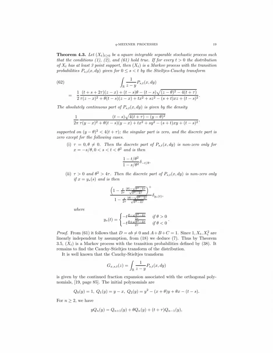
Theorem 4.3. Let (Xt)t≥0 be a square integrable separable stochastic process suchthat the conditions (1), (2), and (61) hold true. If for every t > 0 the distributionof Xt has at least 3 point support, then (Xt) is a Markov process with the transitionprobabilities Ps,t(x, dy) given for 0 ≤ s < t by the Stieltjes-Cauchy transform
∫
R
1
z − yPs,t(x, dy)(62)
=1
2
(t + s + 2τ)(z − x) + (t − s)θ − (t − s)√
(z − θ)2 − 4(t + τ)
τ(z − x)2 + θ(t − s)(z − x) + tx2 + sz2 − (s + t)xz + (t − s)2.
The absolutely continuous part of Ps,t(x, dy) is given by the density
1
2π
(t − s)√
4(t + τ) − (y − θ)2
τ(y − x)2 + θ(t − s)(y − x) + tx2 + sy2 − (s + t)xy + (t − s)2,
supported on (y − θ)2 < 4(t + τ); the singular part is zero, and the discrete part iszero except for the following cases.
(i) τ = 0, θ 6= 0. Then the discrete part of Ps,t(x, dy) is non-zero only forx = −s/θ, 0 < s < t < θ2 and is then
1 − t/θ2
1 − s/θ2δ−t/θ.
(ii) τ > 0 and θ2 > 4τ . Then the discrete part of Ps,t(x, dy) is non-zero onlyif x = y∗(s) and is then
(
1 − t2τ
|θ|−√
θ2−4τ√θ2−4τ
)+
1 − s2τ
|θ|−√
θ2−4τ√θ2−4τ
δy∗(t),
where
y∗(t) =
{
−t θ−√
θ2−4τ2τ if θ > 0
−t θ+√
θ2−4τ2τ if θ < 0
.
Proof. From (61) it follows that D = ab 6= 0 and A+B+C = 1. Since 1, Xt, X2t are
linearly independent by assumption, from (18) we deduce (7). Thus by Theorem3.5, (Xt) is a Markov process with the transition probabilities defined by (38). Itremains to find the Cauchy-Stieltjes transform of the distribution.
It is well known that the Cauchy-Stieltjes transform
Gx,s,t(z) =
∫
R
1
z − yPs,t(x, dy)
is given by the continued fraction expansion associated with the orthogonal poly-nomials, [19, page 85]. The initial polynomials are
Q0(y) = 1, Q1(y) = y − x, Q2(y) = y2 − (x + θ)y + θx − (t − s).
For n ≥ 2, we have
yQn(y) = Qn+1(y) + θQn(y) + (t + τ)Qn−1(y),
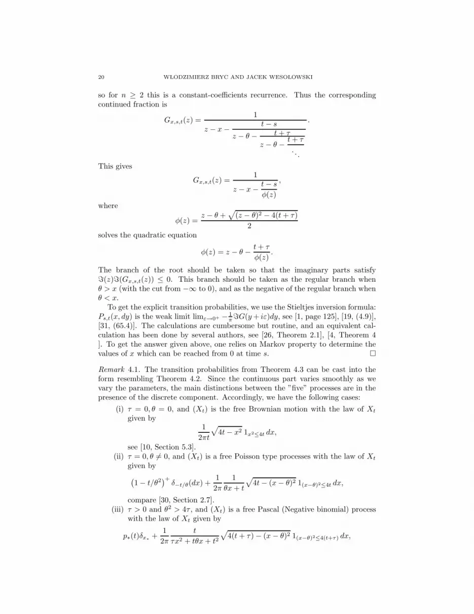
20 W LODZIMIERZ BRYC AND JACEK WESO LOWSKI
so for n ≥ 2 this is a constant-coefficients recurrence. Thus the correspondingcontinued fraction is
Gx,s,t(z) =1
z − x − t − s
z − θ − t + τ
z − θ − t + τ
. . .
.
This gives
Gx,s,t(z) =1
z − x − t − s
φ(z)
,
where
φ(z) =z − θ +
√
(z − θ)2 − 4(t + τ)
2solves the quadratic equation
φ(z) = z − θ − t + τ
φ(z).
The branch of the root should be taken so that the imaginary parts satisfyℑ(z)ℑ(Gx,s,t(z)) ≤ 0. This branch should be taken as the regular branch whenθ > x (with the cut from −∞ to 0), and as the negative of the regular branch whenθ < x.
To get the explicit transition probabilities, we use the Stieltjes inversion formula:Ps,t(x, dy) is the weak limit limε→0+ − 1
πℑG(y + iε)dy, see [1, page 125], [19, (4.9)],[31, (65.4)]. The calculations are cumbersome but routine, and an equivalent cal-culation has been done by several authors, see [26, Theorem 2.1], [4, Theorem 4]. To get the answer given above, one relies on Markov property to determine thevalues of x which can be reached from 0 at time s. �
Remark 4.1. The transition probabilities from Theorem 4.3 can be cast into theform resembling Theorem 4.2. Since the continuous part varies smoothly as wevary the parameters, the main distinctions between the ”five” processes are in thepresence of the discrete component. Accordingly, we have the following cases:
(i) τ = 0, θ = 0, and (Xt) is the free Brownian motion with the law of Xt
given by1
2πt
√
4t − x2 1x2≤4t dx,
see [10, Section 5.3].(ii) τ = 0, θ 6= 0, and (Xt) is a free Poisson type processes with the law of Xt
given by
(
1 − t/θ2)+
δ−t/θ(dx) +1
2π
1
θx + t
√
4t − (x − θ)2 1(x−θ)2≤4t dx,
compare [30, Section 2.7].(iii) τ > 0 and θ2 > 4τ , and (Xt) is a free Pascal (Negative binomial) process
with the law of Xt given by
p∗(t)δx∗+
1
2π
t
τx2 + tθx + t2
√
4(t + τ) − (x − θ)2 1(x−θ)2≤4(t+τ) dx,

q-MEIXNER PROCESSES 21
where
p∗(t) =
(
1 − t
2τ
|θ| −√
θ2 − 4τ√θ2 − 4τ
)+
,
and
x∗(t) =
t(√
θ2 − 4τ − θ)/(2τ) if θ > 0,
−t(√
θ2 − 4τ + θ)/(2τ) if θ < 0,
compare [4, Theorem 4 ].(iv) τ > 0 and θ2 = 4τ and (Xt) is a free Gamma type process with the law of
Xt given by
1
2π
4t
(xθ + 2t)2
√
4t + θ2 − (x − θ)2 1(x−θ)2≤4t+θ2 dx,
compare [4, Theorem 4 ].(v) θ2 < 4τ , and (Xt) is a free Meixner (hyperbolic-secant) type process with
the law of Xt given by
1
2π
t
τx2 + tθx + t2
√
4(t + τ) − (x − θ)2 1(x−θ)2≤4t dx,
compare the “Continuous Binomial process” in [4, Theorem 4 ].
We remark that these measures are closed under the free convolution, L(Xt+s) =L(Xt) ⊞ L(Xt); this is well known, and can be easily seen from the correspondingR-series which for τ > 0 is
RXt(z) = t
1 − zθ −√
(1 − zθ)2 − 4z2τ
2zτ,
compare [11, Proposition 3.4]. The free Brownian and free Poisson processes havebeen studied in considerable detail, see [30] and the references therein. Symmetricfree Meixner distribution appears in [14, Theorem 3], and in [13]. According to [26,Theorem 3.2(2)], these laws are infinitely divisible with respect to the free convolu-tion, with explicit Levy representations. All five distributions occur in Anshelevich[4, Theorem 4]; Anshelevich also points out that the correspondence between theclassical and free Levy processes based on the values of parameters θ, τ does notmatch the Bercovici-Pata bijection.
4.4. Binomial Example. The coefficients in (2) and (6) alone do not determinethe distribution of a process, and (2) and (6) may be satisfied by processes withunivariate distributions different than those listed in Theorem 3.5.
Proposition 4.4. Let p : [0,∞) → [0,∞) be such that∫∞
0p(x) dx < 1. Fix m ∈ N
and let π(s, t) =∫ t
sp(x) dx. The Markov process (Ys)s≥0 with Y0 = 0 and the
transition probabilities
P (Yt = j|Ys = i) =(m − i)!
(j − i)!(m − j)!
(π(s, t))j−i
(1 − π(0, t))m−j
(1 − π(0, s))m−i ,
for 0 ≤ i ≤ j ≤ m and any 0 ≤ s < t, satisfies (2) and (6) with the coefficients thatdo not depend on the parameter m ∈ N. Namely,
(63) E(Yt|F≤s ∨ F≥u) =π(t, u)
π(s, u)Ys +
π(s, t)
π(s, u)Yu

22 W LODZIMIERZ BRYC AND JACEK WESO LOWSKI
and
(64) Var(Yt|F≤s ∨ F≥u) =π(s, t)π(t, u)
(π(s, u))2 (Yu − Ys).
Proof. We first show that the transition probabilities are consistent. For any 0 ≤s < t < u and integers i, n ≥ 0, i + n ≤ m
P (Yu = i + n|Ys = i) =n∑
j=0
P (Yu = i + n|Yt = i + j)P (Yt = i + j|Ys = i)
=
n∑
j=0
(m − i)! (π(t, u ))n−j
(1 − π(0, u ))m−i−n
(π(s, t ))j
j!(n − j)!(m − i − n)! (1 − π(0, s ))m−i
=(m − i)! (1 − π(0, u))m−i−n
n!(m − i − n)! (1 − π(0, s))m−i
n∑
j=0
(
nj
)
(π(s, t))j
(π(t, u))n−j
=(m − i)!
n!(m − i − n)!
(1 − π(0, u))m−i−n
(1 − π(0, s))m−i (π(s, t) + π(t, u))
n.
=(m − i)!
n!(m − i − n)!
(1 − π(0, u))m−i−n
(1 − π(0, s))m−i (π(s, u))
n.
Then the joint distribution of (Ys, Yt, Yu) is given by
P (Yu = i + j + k, Yt = i + j, Ys = i)
= P (Yu = i + j + k|Yt = i + j)P (Yt = i + j|Ys = i)P (Ys = i|Y0 = 0)
=
(
m − i − jk
)
(π(t, u))k
(1 − π(0, u))m−i−j−k
(1 − π(0, t))m−i−j
×(
m − ij
)
(π(s, t))j (1 − π(0, t))m−i−j
(1 − π(0, s))m−i
(
mi
)
(π(0, s))i (1 − π(0, s))m−i
=m!
i!j!k!(m − i − j − k)!(π(0, s))i (π(s, t))j (π(t, u))k (1 − π(0, u))m−i−j−k .
From this, it is easy to see that conditionally on Ys, Yu, the increment Yt − Ys
has the binomial distribution with Yu − Ys trials and the probability of successπ(s, t)/π(s, u), i.e.,
P (Yt = k + i|Ys = i, Yu = i + n) =
(
nk
)(
π(s, t)
π(s, u)
)k (π(t, u)
π(s, u)
)n−k
.
Therefore
E(Yt|Ys, Yu) = Ys +π(s, t)
π(s, u)(Yu − Ys),
and (63) follows from the Markov property. Similarly, (64) is a consequence ofMarkov property and the formula for the variance of the binomial distribution.
�
Remark 4.2. For s ≤ t the conditional distribution of Yt − Ys given Ys is binomialb(m − Ys, π(s, t)/(1 − π(0, s)), which gives
Cov(Ys, Yt) = mπ(0, s) (1 − π(0, t)) .

q-MEIXNER PROCESSES 23
Acknowledgement. Part of the research of WB was conducted while visiting theFaculty of Mathematics and Information Science of Warsaw University of Technol-ogy. The authors thank M. Bozejko for bringing to their attention several references,to Hiroaki Yoshida for information pertinent to Theorem 4.3, and to M. Anshele-vich, W. Matysiak, R. Speicher, P. Szab lowski, and M. Yor for helpful commentsand discussions. Referee’s comments lead to several improvements in the paper.
References
[1] Akhiezer, N. I. The classical moment problem. Oliver & Boyd, Edinburgh, 1965. Russianoriginal: Moscow 1961.
[2] Al-Salam, W. A., and Chihara, T. S. Convolutions of orthonormal polynomials. SIAM J.Math. Anal. 7, 1 (1976), 16–28.
[3] Anshelevich, M. Partition-dependent stochastic measures and q-deformed cumulants. Doc.Math. 6 (2001), 343–384 (electronic).
[4] Anshelevich, M. Free martingale polynomials. Journal of Functional Analysis 201 (2003),228–261. ArXiv:math.CO/0112194.
[5] Anshelevich, M. Appell polynomials and their relatives. Int. Math. Res. Not. 65 (2004),3469–3531. ArXiv:math.CO/0311043.
[6] Anshelevich, M. q-Levy processes. J. Reine Angew. Math. 576 (2004), 181–207.ArXiv:math.OA/03094147.
[7] Anshelevich, M. Linearization coefficients for orthogonal polynomials using stochastic pro-cesses. Annals of Probability 33 (2005). ArXiv:math.CO/0301094.
[8] Askey, R., and Ismail, M. Recurrence relations, continued fractions, and orthogonal poly-nomials. Mem. Amer. Math. Soc. 49, 300 (1984), iv+108.
[9] Askey, R., and Wilson, J. Some basic hypergeometric orthogonal polynomials that gener-alize Jacobi polynomials. Mem. Amer. Math. Soc. 54, 319 (1985), iv+55.
[10] Biane, P. Processes with free increments. Math. Z. 227, 1 (1998), 143–174.[11] Bozejko, M., and Bryc, W. On a class of free Levy laws related to a regression problem.
arxiv.org/abs/math.OA/0410601, 2004.[12] Bozejko, M., Kummerer, B., and Speicher, R. q-Gaussian processes: non-commutative
and classical aspects. Comm. Math. Phys. 185, 1 (1997), 129–154.[13] Bozejko, M., Leinert, M., and Speicher, R. Convolution and limit theorems for condi-
tionally free random variables. Pacific J. Math. 175, 2 (1996), 357–388.[14] Bozejko, M., and Speicher, R. ψ-independent and symmetrized white noises. In Quan-
tum probability & related topics, QP-PQ, VI. World Sci. Publishing, River Edge, NJ, 1991,pp. 219–236.
[15] Bryc, W. A characterization of the Poisson process by conditional moments. Stochastics 20(1987), 17–26.
[16] Bryc, W. Stationary random fields with linear regressions. Annals of Probability 29 (2001),504–519.
[17] Bryc, W., and Plucinska, A. A characterization of infinite gaussian sequences by condi-tional moments. Sankhya A 47 (1985), 166–173.
[18] Bryc, W., Szab lowski, P., and Matysiak, W. Probabilistic aspects of Al-Salam–Chiharapolynomials. Proc. Amer. Math. Soc., to appear.
[19] Chihara, T. S. An introduction to orthogonal polynomials. Gordon and Breach, New York,1978.
[20] Dunkl, C. F., and Xu, Y. Orthogonal polynomials of several variables, vol. 81 of Encyclo-pedia of Mathematics and its Applications. Cambridge University Press, Cambridge, 2001.
[21] Hammersley, J. M. Harnesses. In Proc. Fifth Berkeley Sympos. Mathematical Statistics andProbability (Berkeley, Calif., 1965/66), Vol. III: Physical Sciences. Univ. California Press,Berkeley, Calif., 1967, pp. 89–117.
[22] Matysiak, W., and Szab lowski, P. A few remarks on Bryc’s paper on random fields withlinear regressions. Ann. Probab. 30, 3 (2002), 1486–1491.
[23] Neu, P., and Speicher, R. Spectra of Hamiltonians with generalized single-site dynamicaldisorder. Zeitschrift fr Physik B Condensed Matter 95 (1994), 101–111.

24 W LODZIMIERZ BRYC AND JACEK WESO LOWSKI
[24] Plucinska, A. On a stochastic process determined by the conditional expectation and theconditional variance. Stochastics 10 (1983), 115–129.
[25] Saitoh, N., and Yoshida, H. q-deformed Poisson random variables on q-Fock space. J.Math. Phys. 41, 8 (2000), 5767–5772.
[26] Saitoh, N., and Yoshida, H. The infinite divisibility and orthogonal polynomials with aconstant recursion formula in free probability theory. Probab. Math. Statist. 21, 1, ActaUniv. Wratislav. No. 2298 (2001), 159–170.
[27] Schoutens, W. Stochastic processes and orthogonal polynomials, vol. 146 of Lecture Notesin Statistics. Springer-Verlag, New York, 2000.
[28] Shohat, J. A., and Tamarkin, J. D. The problems of moments, vol. 1 of Math. Surveys.American Math. Soc., New York, 1943, 1950.
[29] Szab lowski, P. J. Can the first two conditional moments identify a mean square differentiableprocess? Comput. Math. Appl. 18, 4 (1989), 329–348.
[30] Voiculescu, D. Lectures on free probability theory. In Lectures on probability theory andstatistics (Saint-Flour, 1998), vol. 1738 of Lecture Notes in Math. Springer, Berlin, 2000,pp. 279–349.
[31] Wall, H. S. Analytic Theory of Continued Fractions. D. Van Nostrand Company, Inc., NewYork, N. Y., 1948.
[32] Weso lowski, J. A characterization of the gamma process by conditional moments. Metrika
36, 5 (1989), 299–309.[33] Weso lowski, J. Stochastic processes with linear conditional expectation and quadratic con-
ditional variance. Probab. Math. Statist. 14 (1993), 33–44.[34] Williams, D. Some basic theorems on harnesses. In Stochastic analysis (a tribute to the
memory of Rollo Davidson). Wiley, London, 1973, pp. 349–363.
Department of Mathematics, University of Cincinnati, PO Box 210025, Cincinnati,
OH 45221–0025, USA
E-mail address: [email protected]
Faculty of Mathematics and Information Science, Warsaw University of Technol-
ogy, pl. Politechniki 1, 00-661 Warszawa, Poland
E-mail address: [email protected]


