Department of Economics and Finance

RoME Master in Economics by Luiss ”Guido Carli” & Eief

Chair: Asset Pricing

Conditional Risk Premia in The

Consumption-CAPM

Prof. Nicola BorriSupervisor

Prof. Pietro ReichlinCo-Supervisor

Daniel MeleMatr. 707891Candidate

Academic Year: 2019/2020

Conditional Risk Premia in The Consumption-CAPM

RoME Master in Economics by Luiss ”Guido Carli” & Eief

Daniel Mele

Abstract

In this paper, the results obtained by Lettau, Maggiori, and Weber (2014) in their seminal paper,

Conditional Risk Premia in the Currency Markets and Other Asset Classes, are extended to the

classical consumption capital asset pricing model. The quantity of risk estimated is higher

conditional on low states of the world and the difference with the unconditional beta is able

to capture an important dimension of risk. Indeed, including the downside risk increases the

empirical performance of the model and reduce the pricing errors for currency, commodity, and

equity portfolios. However, only the market factor is able to price the whole cross-section of

returns.

Acknowledgements

I thank all the people that in this early stage of my journey have supported my efforts. First

of all, I will be always grateful to my family, their solid belief in me and their sacrifices for this

moment have always guided my walk. Right after, I cannot forget all the amazing friends that I

have met along the way. Alessandro, Alfredo, Andrea, Carlo, Jessica, Leonardo e Salvatore have

shown me that friendship is not a matter of time spent together but of shared views. Words

are not sufficient to thank my ”colleagues”, both my high school and master classes have been

the best groups I would have ever dreamed of. Thanks to them I don’t know what is loneliness.

Last but not least, often I have not walked with my own legs but Luisa Greta has carried the

burden of my particular temperament, her unconditional presence has positively inspired me

and my choices. So I beat on, boat against the current.

1

2

Contents

1 Introduction 5

2 Econometric framework 7

2.1 Modified Two-step Fama-MacBeth Regression . . . . . . . . . . . . . . . . . . . . . . 8

2.2 Model performance evaluation . . . . . . . . . . . . . . . . . . . . . . . . . . . . . . . 9

3 Data & Descriptive Statistics 11

3.1 Conditional Correlations . . . . . . . . . . . . . . . . . . . . . . . . . . . . . . . . . . 15

4 Empirical Results 17

4.1 Currencies . . . . . . . . . . . . . . . . . . . . . . . . . . . . . . . . . . . . . . . . . . 17

4.2 Fama and French . . . . . . . . . . . . . . . . . . . . . . . . . . . . . . . . . . . . . . 20

4.3 Commodities . . . . . . . . . . . . . . . . . . . . . . . . . . . . . . . . . . . . . . . . 22

5 Pricing the Cross-section 24

5.1 Principal component evidence . . . . . . . . . . . . . . . . . . . . . . . . . . . . . . . 24

5.2 Results . . . . . . . . . . . . . . . . . . . . . . . . . . . . . . . . . . . . . . . . . . . . 25

6 Evidence from the COVID-19 crisis 28

6.1 Industry portfolios analysis . . . . . . . . . . . . . . . . . . . . . . . . . . . . . . . . 28

6.2 Prediction . . . . . . . . . . . . . . . . . . . . . . . . . . . . . . . . . . . . . . . . . . 29

7 Robustness checks 30

7.1 Downside definition . . . . . . . . . . . . . . . . . . . . . . . . . . . . . . . . . . . . . 30

7.2 Predictability of consumption growth . . . . . . . . . . . . . . . . . . . . . . . . . . . 32

8 Conclusion 34

9 References 35

Appendix A: Time series properties 37

Appendix B: Principal component analysis 38

3

4

1 Introduction

The classical capital asset pricing model is based on the covariance between asset and market returns

as the investor does not want to see the market crushing together with the particular asset. However,

traditional risk factors as the market and consumption factors have been criticized recurrently in

the asset pricing literature. Low predictive power and inability to estimate different assets classes

are major drawbacks highlighted during several decades. Despite this, the research to reconcile the

discount factors with assets return is still fervid and ongoing. The aim and importance of this agenda

can be summarized with the words of Cochrane (2011)[6] in his speech at the American Finance

Association: ”What is the factor structure of time-varying expected returns? Expected returns vary

overtime. How correlated is such variation across assets and asset classes? How can we best express

that correlation as factor structure?. . . This empirical project has just begun,. . . but these are the

vital questions.”

Building on Ang, Chen and Xing (2006)[1], Lettau, Maggiori and Weber(2014)[13], hereafter

LMW, showed that the conditional risk, the risk to be riskier in bad times, is able to reconcile

the market factor with several asset classes and to price a cross-section of asset returns, thereby

improving upon the existing asset specific models which have failed to price it accurately. Conditional

risk concerns the downside periods that the investors face. The covariance with the chosen factor

captures an important dimension of risk but, the asymmetry in normal and bad times can play

a key role in the determination of the excess returns required by the market. The intuition is

straightforward and with a long tradition in the literature (Markowitz 1959[17]). Assets that co-

move in bad times are riskier given the high marginal utility of substitution present in downside

periods. This generates an automatic question regarding the behavior of the consumption factor

with the addition of conditional risk given the close connection between consumption growth and

linear pricing models in the economic literature.

The aim of this article is to replicate the empirical framework developed by LMW[13] to test

the ability of downside risk to reconcile the consumption factor with asset returns. The standard

consumption capital asset pricing model of Lucas (1978)[14] and Breeden (1979)[2] is estimated with

an additional factor to account for conditional risk. The estimation is carried with the LMW[13]

methodology both in the estimation of the quantities and prices of risk and in the definition of the

downside periods. In particular, the downside is identified in any period for which the factor is one

standard deviation below its sample mean. This assumption is robust to several checks and allows

to balance the need for variability and real risk that requires an high and low threshold respectively.

5

In order to test the model three main asset classes are considered. Firstly, a cross-section of

currencies returns is considered to have comparable results to the original work of LMW[13] where

this asset was particularly sensitive to the inclusion of downside periods due to the co-movements

of the carry trade strategy with the market returns. Next, a broadly used measure of equity returns

represented by the six Fama-French portfolios sorted on book-to-value and size is tested to have

results comparable to different models. Lastly, estimation is carried for commodity returns given

that also the so called basis trade has been proved to be sensitive to the conditional risk, Yang

(2013)[21]. Furthermore, the consumption variable is constructed to be closer as possible to the

micro-founded framework and is defined as the personal expenditure for non-durables and services.

Standard assumption of i.i.d consumption growth time series is tested for robustness.

Results show a picture quite uniform. Conditional risk is unable to replicate the increase in

performance of the capital asset pricing model (CAPM). In particular, against an average 40%

decrease in pricing error for CAPM, the consumption-CAPM delivers a 10% decrease. However,

minor heterogeneity across different asset classes and individual results are reported. The main

conclusion regards the failure of the conditional risk to price the whole cross-section of test assets

differently from the LMW[13] contribution. Indeed, while a positive and significant conditional price

of risk (1.4) is present for the CAPM, the Consumption-CAPM delivers a non significant and close

to zero estimate for it. The results are robust to various checks and, to have a more transparent

comparison, standard results for the CAPM containing the no-arbitrage condition for market return

are reported together with unrestricted estimation due to the absence of a restricted value for the

unconditional price of risk for the Consumption-CAPM

To further investigate the performance of the model an out-of-the sample analysis is conducted.

In particular, predicted Fama-French 5 industry portfolios’ returns are compared against actual

returns under different scenario including the recent Covid19 crisis. The results suggest that the

conditional risk improvement for the performance of the standard linear pricing models is heteroge-

neous depending on the nature of the crisis.

The work is organized as follow. Sec.2 illustrates the econometric framework for the estimation

and the model performance evaluation. Sec.3 contains information regarding data and their main

descriptive. Sec.4 reports results for each individual asset class. Sec.5 reports results for the cross-

section of asset returns with the addition of a principal component analysis. sec.7 contains the

result for the Covid crisis. Sec.7 contains the robustness checks carried out. Sec.8 summarizes the

main conclusions.

6

2 Econometric framework

The simultaneous presence of unconditional and downside risk derives from the intuition that assets

whose returns covary positively with risk factors are riskier but, a stronger covariance conditional on

downside periods identifies an important difference in this riskiness. Indeed, the idea of downside risk

is widespread and recurrent in the asset pricing literature. Classical examples using market return

as risk factor are the concept of ”semi-variance” by Markowitz (1959)[17] or Ang, Chen and Xing

(2006)[1]. Regarding consumption based models, starting from the seminal works of Lucas (1978)[14]

and Breeden (1979)[2] on the CCAPM, the idea of conditional risk-premia is even more pervasive

as the standard assumptions on utility function deliver an higher marginal utility of intertemporal

substitution when consumption is low. Examples of models incorporating this feature are Cochrane

(1996)[4] and Lettau and Ludvigson (2001)[12]. Finally, contributions in the behavioral economics

literature as Kahneman and Tversky’s (1979)[20] have highlighted how loss aversion preferences are

important in modeling investment decision.

The analysis is carried out through the econometric framework suggested by LMW[13]. The

downside-risk factor pricing model with risk factor fa specifies for N expected returns the following

relation

E (ri) = βi,aλa + (β−i,a − βi,a)λ−a , i = 1, · · · , N (1)

β−i,a =Cov (ri, fa)

V ar (ra)

β−i,a =Cov (ri, fa|fa < δ)

V ar (ra|fa < δ)

a = market excess return (m), consumption growth (c)

In particular, ri is the log excess return of asset i over the risk-free rate, βi,a and β−i,a are the

unconditional and downside beta depending on δ, the exogenous threshold defining the ”downside”

period, λa and λ−a are the unconditional and conditional price of risk. In the this context, fm = rm is

the market log excess return identifying the capital asset pricing model (CAPM) and the downside-

risk capital asset pricing model (DR-CAPM) while, fc = ∆c is the consumption growth identifying

consumption-CAPM (CCAPM) and downside-risk consumption-CAPM (DR-CCAPM).

The model shrinks to the correspondent classical one-factor model if the covariance is symmetric

in good and bad periods i.e. βi,a = β−i,a, or the conditional market risk is zero, i.e. λ−a = 0. LMW

[13] impose the restriction that the market return is exactly priced given standard assumption of no-

7

arbitrage on the market. However, the comparison between CCAPM and CAPM behaviors including

the downside risk is more transparent if we check that result for CAPM are robust relaxing the no-

arbitrage condition because in the case of CCAPM the unconditional price of risk does not have a

predetermined restricted version. Therefore, during the analysis, restricted (R) and unresticted (UR)

models are reported. Following Cochrane (2009)[5], the price of risk for the restricted specifications

of the CAPM is simply the expected market excess return given that the market is always perfectly

correlated with itself. When the risk factor does not report a standard error in the estimation it

means that it’s not estimated but restricted.

λm = ET [rm]

The model does not allow to have time-varying coefficients but incorporates the conditional risk

with a multiple factor specification. Even if this restriction can undermine the performance of the

model, the results are conservative because in short sample periods, contemporaneous presence of

multiple factors and time-varying coefficients leads to few observations available in the downstate

periods and low efficiency.

2.1 Modified Two-step Fama-MacBeth Regression

The estimation of the econometric model is implemented with a modified version of the standard

Fama and MacBeth (1973)[10] procedure. Given N time-series of assets returns and a time-series

for market return and consumption growth, in the first stage N × 2 time-series regressions deliver a

β and a β− for each asset (portfolio, single stocks, derivatives etc...),

rit = ai + βift + εit, ∀t ∈ T (2)

rit = a−i + β−i ft + ε−it , ∀t : ft ≤ δ (3)

where ft represents the factor used, market log excess return for the CAPM and consumption

growth for the CCAPM. Specifically, this stage extend the classical approach estimating the time

series regression only for the observations where the contemporaneous factor is below the defined

threshold identifying the downside.

8

The second stage is based on a single cross-section regression with N observations

E[ri] = β̂i,aλa + (β̂−i,a − β̂i,a)λ−a + αi (4)

The regression takes as regressors the estimated quantity of risk β, β− for each asset and find the

price of risk λ− and λ when the latter is not restricted in the CAPM case. However, these estimates

do not take into account the possible correlation in the panel. Regarding auto-correlation, the

assumption that asset returns time series are not highly correlated is not a major source of concern

as the literature has proved (see Cochrane 2009 [5] chapter 12). Most harmful is the assumption

about cross-sectional correlation in the panel. To avoid low estimates of the standard errors of

our estimated prices of risk, the standard Fama-MacBeth (1973)[10] correction is implemented. In

particular, the second-step cross-sectional regression is estimated at each sample period. Firstly,

the estimated prices of risk λ, λ− are computed as the average of the T cross-sectional regressions

estimates.

λ̂ =1

T

T∑t=1

λ̂t, λ̂− =1

T

T∑t=1

λ̂−t

Next, the standard deviation of these estimates is used to generate the sampling errors. The intuition

is to use the variation over time of our estimated λs to deduce their possible variation across samples.

Formally, the sampling errors become

σ(λ̂) =

√√√√ 1

T 2

T∑t=1

(λ̂t − λ̂), σ(λ̂−) =

√√√√ 1

T 2

T∑t=1

(λ̂−t − λ̂−)

which coincide, for T sufficiently big, directly with the standard errors of the means λ̂ and λ̂−.

Lastly, in these steps we cannot internalize the fact that also the quantities of risk are estimated

given that the standard Shanken (1992)[19] correction is not feasible due to a double time-series

regression in the first stage. The specification is completed by the threshold δ definition discussed

in Sec.3.

2.2 Model performance evaluation

The estimated β-pricing models have to be validated with data. Therefore, their performance is

assessed under different standard measures. A necessary but not sufficient condition for the success

9

of the model is that the resultant pricing errors are sufficiently small. Following LMW[13], the first

indicator used is the root mean squared pricing errors (RMSPE). During the analysis the reported

values come from monthly percentage errors defined as difference between actual and predicted data.

Hence, a positive error has the interpretation of an under-prediction of the model.

RMSPE =

√√√√ 1

N

N∑i=1

α2i

Another useful information is delivered by the χ2-test that all the pricing errors are jointly zero.

The test null hypothesis is that all errors are zero and therefore a p-value above 5% implies that

the model is not rejected at 5% confidence level. While small differences in p-values are difficult

to read due to possible sampling error, a much higher p-value is an indicator of the goodness of

fit and performance of the model. The test statistic is constructed following Cochrane (2009)[5].

Defining with αt the vector of pricing errors estimated at each point in time of the second step

multiple cross-sectional regression, two main variables are identified, the average pricing errors and

the correspondent covariance.

α̂ =1

T

T∑t=1

α̂t,

cov(α̂) =1

T 2

T∑t=1

(α̂t − α̂)′(α̂t − α̂)

The test is implemented knowing the following result:

α̂′cov(α̂)−1α̂ ∼ χ2N−1

Lastly, the single cross-sectional R2 is reported together with the definition used by LMW [13] to

have comparable results, i.e.

R2LMW = 1− α̂′α̂[NV ar(r)]−1

where r is the vector of the N mean returns of the tested assets. Often, this value takes large

negative values as the standard models spectacularly fail in pricing the cross-section.

10

3 Data & Descriptive Statistics

The dataset for this article is retrieved from multiple public available data. The monthly U.S.

consumption data is obtained from the ’National Income and Product Accounts of the United

States’ (NIPA tables), the population level from the ’Current Population Survey’, both collected by

the U.S. Bureau of Economic Analysis and downloaded through the FRED, Federal Reserve Bank of

St. Louis portal. The monthly excess returns for currencies, equity, and commodities are obtained

from the journal website where LMW [13] uploaded a replicating dataset. The sample period stars

in January 1974 and ends in March 2010 for a total of 435 observations with the exception of the

commodity returns ending in December 2008 (420 observations).

Consumption is defined as the sum of non-durable and services (PCEND1,PCES2) reducing

the measurement problem between expenditures and actual consumption, as remarked by Hall

(1978)[11]. Both time series are released at the aggregate U.S. level in billions of dollars, seasonally

adjusted annual rate. Services account for about 70% of the constructed measure of consumption.

Population used to calculate the per capita numbers is the civilian non-institutional population

(CNP16OV3) reported in thousands and defined as ”a person 16 years of age and older residing in

the 50 states and the District of Columbia, who are not inmates of institutions (e.g., penal and men-

tal facilities, homes for the aged), and who are not on active duty in the Armed Forces”. Throughout

the analysis consumption is interpreted with the beginning-of-period convention following Engsted

and Moller (2015)[8] that remarks the striking difference between beginning and end of period con-

ventions’ for the performance of CAPM. Basically, the consumption reported on national account

for a particular month is interpreted as the flow occurred the period before.

The market return is the value-weighted Center for Research in Security Prices (CRSP) US equity

market log excess return. The use of this broad definition of market is common in the literature and

conservative in avoiding automatic increase in the correlation with the non-equity test assets and

the market risk factor.

Fig.1 shows the time series of the two risk factors. Even if market excess return is more volatile,

the two series present a similar number of downside periods (vertical lines). Table.1 quantifies

this similarity showing that the percentage of downside periods for the market excess return and

1U.S. Bureau of Economic Analysis, Personal Consumption Expenditures: Nondurable Goods [PCEND], retrievedfrom FRED, Federal Reserve Bank of St. Louis; https://fred.stlouisfed.org/series/PCEND

2U.S. Bureau of Economic Analysis, Personal Consumption Expenditures: Services [PCES], retrieved from FRED,Federal Reserve Bank of St. Louis; https://fred.stlouisfed.org/series/PCES

3U.S. Bureau of Labor Statistics, Population Level [CNP16OV], retrieved from FRED, Federal Reserve Bank ofSt. Louis; https://fred.stlouisfed.org/series/CNP16OV

11

the consumption growth are 12.6% and 10.1% on the full sample respectively (55 and 44 periods).

Moreover, the variability of the consumption factor is around one fourth of the market factor in

line with the empirical research showing the low variation using consumption series (Mankiw and

Shapiro 1986) [16]. Regarding growth rates, the per-capita consumption shows an annualized 0.5%

growth rate with population explaining only about 20% of this trend. The standard deviation of

0.4% and the range of 0.3% clearly illustrates of the dispersion of this measure. Again, the latter

consideration is more prominent for market excess return (annualized mean 4.7 % and standard

deviation 16.5%).

In line with the previous literature, the two factors are interpreted as new information connected

to investors decisions. Clearly, the time-series properties of both deliver an useful insight in in-

terpreting the results. Sec.7 and Appendix A investigate on the standard assumption of i.i.d

consumption growth time-series (Cochrane 2009[5]).

Table 1: Risk Factors DescriptiveThe table reports annualized rate, standard deviation and percentiles for market excess return based on CRSP-US

equity return and personal consumption growth rate. Consumption is defined as the sum of non-durables and services.

The percentage of observation where the factor is one standard deviation below the sample mean is included. The

sample period is January 1974 to March 2010 for a total of 435 observation.

Mean StandardDeviation

DownsidePeriods

Median 25pct 75pct

AnnualizedGrowth RatePer-Capita Consumption 0.465 0.406 10.11% 0.437 0.227 0.694

AnnualizedExcess ReturnMarket Factor 4.668 16.469 12.64% 10.990 −26.695 41.977

Equity returns are based on the six Fama and French portfolios sorted on size and book-to-

market publicly available on Kenneth French Website4. Table.2, panel A, reports the standard

result regarding higher excess returns for small and value stocks, Fama and French (1992)[9]. The

currencies returns covering 53 countries are sorted in six portfolios based on their interest rate

following Lustig and Verdelhan(2007) [15] and excluding high inflation countries (annualized monthly

inflation 10% higher than U.S. annualized monthly inflation in the same month). The returns are

calculated by LMW[13] adding the interest rate differential and the rate of exchange rate depreciation

with the US dollar

rt+1 = it − iust −∆st+1

4http://mba.tuck.dartmouth.edu/pages/faculty/ken.french/datalibrary.html

12

Table.2, panel B, shows that this sorting based on interest rate differential generates an increasing

cross-section of portfolios’ returns confirming the standard strategy behind the carry trade, long in

high differential currency and short in low differential currency yields positive excess returns. Lastly,

the cross-section of commodities is based on five futures portfolios sorted by the commodity basis by

Yang (2013)[21]. The basis of a commodity is the difference between the futures price and the spot

price of that commodity. Similarly, a basis trade strategy long in low basis and short in high basis

currencies has shown to deliver positive excess returns. Table.2, panel C, shows that the sorting

generates a decreasing cross-section of portfolios returns as discussed.

The focus on equity, currencies and commodities is driven by their central role in the LMW[13]

work and therefore, they are used to have a more transparent comparison of the different β−pricing

models.

Table 2: Test Assets StatisticsThe table reports annualized sample means, standard deviations, and Sharpe ratios for portfolios of equity, currency,

and commodity excess returns. Panel A reports the statistics for the six Fama-French portfolios sorted on size and

book-to-value. Panel B reports the statistics for six monthly re-sampled currency portfolios based on the interest rate

differential with the US. Panel C reports the statistics for five commodity portfolios monthly re-sampled based on

the basis. The sample period is January 1974 to March 2010 for a total of 435 observations in Panels A and B and

January 1974 to March 2008 for a total of 420 observations in Panel C

Mean StandardDeviation

SharpeRatio

Panel A: Fama-French 6-portfoliosSmall sizeLow book-to-market 3.232 24.553 0.132Medium book-to-market 9.796 18.857 0.519High book-to-market 11.508 19.526 0.589

Big sizeLow book-to-market 3.945 17.181 0.230Medium book-to-market 5.664 15.758 0.359High book-to-market 6.783 16.638 0.408

Panel B: Currency portfoliosLow -2.517 7.731 -0.3262 0.795 7.637 0.1043 0.690 7.765 0.0894 2.355 7.215 0.3265 2.867 8.127 0.353High 4.936 10.731 0.460

Panel C: Commodity portfoliosBasisLow 9.184 18.504 0.4962 5.697 15.647 0.3643 3.595 16.378 0.2194 0.318 15.576 0.0205 −0.132 17.342 −0.008

13

(a) Consumption growth

(b) Market excess return

Figure 1: Risk Factors Time-SeriesOutlined are the risk factors time-series with vertical lines representing ”downside” periods, one standard deviation

below the sample mean. The top panel shows the time-series for the personal consumption growth rate factor.

Consumption is defined as the sum of non-durables and services. The bottom panel shows the time-series for the

market excess return defined as the CRSP-US equity return. The sample period is January 1974 to March 2010 for a

total of 435 observation.

14

In particular, carry and basis trades are crucial strategies analyzed for the understanding of

the performance of the downside risk (Burnside (2011)[3], Yang (2013)[21]). Nevertheless, they

represent classes broadly used in the finance literature and of general interest, with the Fama and

French portfolios being the standard choice to test asset pricing models. Table.2 reports, in addition

to the annualized mean returns, the sample standard deviation and Sharpe ratio for these three test

assets.

3.1 Conditional Correlations

The performance of the downside risk pricing model is intrinsically related to the evidence that some

cross-section strategies are more highly correlated with the risk factor chosen whenever the riskiness

is higher. Similarly to this work, Dobrynskaya (2014)[7] stressed the state dependent behavior of

the carry trade strategy in its co-movement with the market return. However, systematic evidence

across several assets’ classes is scarce and LMW [13] are among the first to explore this idea in a

longer time horizon. Therefore, the contribution given by the response that the CCAPM delivers

considering downside risk is helpful and constructive to find new patterns to reconcile micro-founded

models and empirical evidence. Moreover, ad hoc models that perform well with particular assets

are useful in prediction but interpretation and external validity of the results is difficult. A common

framework based on utility maximization allows to explain what is happening.

The definition of downstate periods is pivotal to the analysis. Two main aspects have to be

considered. First, the threshold has to realistically give rise to economic concerns, i.e. a sufficient

low threshold is required. However, a minimum level of variability in the data is required to have a

sufficiently large sample, i.e. a sufficiently high threshold is required. Defining the downstate as a

period in which the risk factor is at least one standard deviation under its sample mean, is a middle

ground to accommodate both requirements (LMW[13]).

δ = f̄a − σa (5)

In the full sample, we have 44 and 55 periods of downstate out of 435 total periods for consumption

growth and market return respectively. Sec.7 investigates if the results are robust to a different

measure of δ. In particular, all the observations below an half standard deviation from the mean

are considered downside periods in this robustness check.

Table.3 reports sample correlations for three cross-section strategies. They are constructed

15

subtracting the lowest return portfolio from the highest return portfolio. While for currency and

commodities this synthesizes a carry and basis trade, for equity this strategy tries to simulate a

growth-size strategy where the investor is long in a high book-to-market & small size and short in a

low book-to-market & big size to pursuit a positive excess return. Table.3, Panel A, highlights the

correlations for the equity based strategy. Fistly, we can see that the asymmetry between downstate

and upstate. The consumption growth factor shows that the conditional correlations is stronger

in bad states (0.09 vs 0.01) despite a low unrestricted correlation of 0.05 as our basic intuition

suggests. Similarly for the market factor, the asymmetry is present and of the expected sign but

with an amplified effect (0.32 vs −0.11). Table.3, Panel B, gives the same information for the carry

trade. In this case the market factor seems to outperform the consumption factor for which a strong

asymmetry seems not to be present (−0.02 vs 0.03) due to a general low correlation of 0.04. Indeed,

with a conditional correlations of 0.33 in bad state against a conditional correlation of 0.02 in good

state, the carry trade suits the downside risk framework as highlighted in table 4 of LMW[13].

Table 3: Conditional CorrelationsThe table reports correlations between an equity, currency and commodity based strategy and market excess return

and consumption growth. The correlation are measured in full, downside and upside sample periods. Downside is an

observation one standard deviation under the sample mean. The upside is an observation not in the downside period.

The sample period is January 1974 to March 2010 for a total of 435 observations.

All Downstate UpstatePanel A: Fama-French 4 - 3 portfolioMarket factor −0.017 0.315 −0.107

(0.048) (0.130) (0.051)Consumption factor 0.052 0.090 0.012

(0.048) (0.154) (0.154)

Panel B: Carry Trade for currenciesMarket factor 0.137 0.326 0.019

(0.048) (0.130) (0.051)Consumption factor 0.041 −0.017 0.029

(0.048) (0.154) (0.154)

Panel C: Basis Trade for commoditiesMarket factor −0.055 0.186 −0.070

(0.049) (0.138) (0.052)Consumption factor 0.011 −0.161 −0.011

(0.049) (0.160) (0.162)

Lastly, Table.3, Panel C, delivers estimate of the correlations for the basis trade. For both

models the asymmetry is present with a similar magnitude (0.19 vs −0.07 and −0.16 vs −0.01 for

market and consumption respectively) even with an unrestricted correlation close to zero (−0.05 for

the market factor and 0.01 for the consumption factor).

16

4 Empirical Results

The main finding in the analysis developed is the positive but smaller impact of the downside risk

for the consumption-CAPM respect to the market counterpart represented by the classical CAPM.

Fig.2 summarizes this result plotting average improvements between the two models. Specifically,

the mean pricing error (RMSPE) is the average error across the three test assets used. While the

CAPM has a reduction of this measure around the 40%, the DR-CCAPM slightly decreases the

error of the CCAPM only by 10%. However, this difference varies significantly across the test assets.

Therefore, specific results for currencies, Fama and French portfolios and commodities are reported.

Figure 2: Average ImprovementsOutlined are the average improvements for two β-pricing model with an additional downside risk specification for both.

The performance is based on the root squared pricing error (RMSPE) that is averaged out across equity, currency

and commodities portfolios. The sample period of these test assets is January 1974 to March 2010 for a total of 435

observations for the equity and currency assets and January 1974 to December 2008 for the commodity assets for a

total of 420 observations.

4.1 Currencies

The first row of Fig.3 reports the evidence proposed by LMW[13] to explain the positive impact

of the downside risk in predicting carry trade returns. The up-left panel shows how the variation

in beta is not able to explain the variation in mean returns. However, the up-middle panel starts

to highlight how an higher covariance in bad times better explain the returns dispersion. This is

17

not sufficient to claim failure of the CAPM given that assets that covary more in bad times can

covary more also in good times i.e. no asymmetry. Therefore, up-right panel is the key point to

understand the mechanism. The relative downside beta (β− − β) captures the market conditional

risk and indeed an increasing distribution of returns appears with the rise in conditional risk. How

this translates when consumption is used as risk factor is the question under investigation.

The second row of Fig.3 repeats the analysis using the quantities of risk associated with the

consumption factor. Similarly to its one-market-factor counterpart, the down-left panel explains the

striking failure of the CCAPM. Dispersion is too narrow respect to actual returns. Again, down-

middle and down-right panels put under the light the impact of the conditional risk. The plots convey

a similar results as discussed for the CAPM but the results are not of the same magnitude. Even

if an increase in the dispersion of betas and relative betas is present, the pattern is not monotonic

and some portfolios diverges remarkably from what is expected.

Figure 3: Risk-return relations: CurrenciesOutlined are risk–gain relations for six monthly re-sampled currency portfolios (1 to 6), based on the interest rate

differential with the US. The panels plot the mean excess return against several different betas. The sample period is

January 1974 to March 2010 for a total of 435 observations.

Fig.4 and Table.4 depict and quantify respectively the performance of the models under discus-

sion for currencies portfolios. Firstly, we see in the left and middle columns of Fig.4 that relaxing

the no-arbitrage condition on the market excess return has no significant impact on the performance

18

of the model. Coherently with the basic intuition of the econometric model, the single factor models

are not able to capture the risk-return trade-off and predict basically the same return for each port-

folio. First row of Fig.4 shows this failure. Adding the downside risk in the second row improves

the performance as the returns are close to the 45 degree line as desired but, the consumption factor

does not deliver a striking improvement as the market one.

Figure 4: Model performance: CurrenciesOutlined are annualized mean excess returns against the predicted excess returns in percent for several β-pricing

models. Test assets are six monthly re-sampled currency portfolios (1 to 6), based on the interest rate differential

with the US. The market excess return is included as a test asset (0). The sample period is January 1974 to March

2010 for a total of 435 observations.

Table.4 reports the estimated prices of risk. Again, the results are not driven by the restriction

imposed on the market return. Notably, the unrestricted models has difficulties in estimating the

unrestricted price of risk but they deliver positive and significant downside risk, 2.18 and 0.13 for

the CAPM and CCAPM respectively. While the one factor models show a similar magnitude of

pricing error, captured by the RMSPE, the additional factor halves the error for the CAPM and

decreases the CCAPM error pricing just by 15%. On the other hand, excluding the unrestricted

downside risk-CAPM (p-value 58%), all models are rejected by the assumption of jointly pricing

errors equal to zero. and have portfolio 1 with the highest pricing error. Comparing the explained

variability, the CAPM gives a greater insight always but the conditional improvement is relatively

more important for the CCAPM with a tenfold increase.

19

Table 4: Estimation of linear pricing model: CurrenciesThe table reports prices of risk, χ2 statistics testing for joint significance of pricing errors, root mean squared pricing

errors (RMSPE), the number of observations T, cross sectional R2’s and the definition of R2 used by LMW [13]

for several β-pricing models. Test assets are six monthly re-sampled currency portfolios, based on the interest rate

differential with the US. The market excess return is included as a test asset. The sample period is January 1974

to March 2010 for a total of 435 observations. Fama and MacBeth standard errors in parentheses. Restricted (R)

models have no standard error for the constrained factor or standard R2 reported.

R R-DR UR UR-DR UR UR-DRCAPM CAPM CAPM CAPM CCAPM CCAPM

λ 0.389 0.389 0.459 0.397 0.061 −0.280(−) (−) (0.231) (0.786) (0.131) (0.196)

λ− 2.181 2.175 0.133(0.772) (0.764) (0.067)

χ2 42.283 24.605 30.870 4.680 27.990 49.771P-value 0.00 0.04 0.01 0.58 0.01 0.00RMSPE 0.191 0.092 0.189 0.092 0.255 0.221R2 (-) (-) 46.67% 87.33% 2.69% 26.67%R2

LMW 8.77% 78.74% 23.37% 81.80% −39.84% −5.39%T 435 435 435 435 435 435

4.2 Fama and French

The first row of Fig.5 reports the evidence proposed by LMW[13] to explain the positive impact

of the downside risk in predicting equity returns. Indeed, from the left to the right, the dispersion

increases using the downside-conditional risk and an higher exposure to the risk is associated to an

higher return. The relative downside beta (β− − β) has the key role in the interpretation.

The second row of Fig.5 exploits the quantities of risk associated with the consumption factor.

The comments to be made are similar to the currencies case with results that are not of the same

magnitude of the CAPM. An increase in the dispersion of betas is present with a not monotonic

behavior. Differently from currencies, we have a more homogeneous pattern for the portfolios but a

general lower dispersion.

Fig.6 plots the performance of the different models for the equity portfolios used. Firstly, the

improvement with the downside risk included is clear for the CAPM case with and without restriction

(again not relevant for the results). On the other hand, the CCAPM shows that the conditional

risk is not able to provide explanatory power as the dispersion across the 45 degrees line is rather

unchanged. However, the CCAPM and DR-CCAPM seems to be more trustworthy respect to the

one-factor market based models.

20

Figure 5: Risk-return relations: Fama and FrenchOutlined are risk–gain relations for the six Fama and French portfolios sorted on book-to-market and size (1 to 6).The

panels plot the mean excess return against several different betas. The sample period is January 1974 to March 2010

for a total of 435 observations.

Figure 6: Model performance: FF PortfoliosOutlined are annualized mean excess returns against the predicted excess returns in percent for several β-pricing

models. Test assets are the six Fama and French portfolios sorted on book-to-market and size (1 to 6). The market

excess return is included as a test asset (0). The sample period is January 1974 to March 2010 for a total of 435

observations.

21

Table.5 reports the estimatation results for the equity portfolios. Differently from the currencies

case, the estimated downside price of risk is not significantly different from zero and actually negative.

This seems to suggest that the consumption conditional risk is not a measure of risk captured by

stock market when sorted by size and book-to-market value. All model are rejected by the hypothesis

of jointly zero pricing errors. The magnitude of RMSPE is similar across all models suggesting that

also the market factor is weaker respect to the currencies case. Remarkably, the additional factor as a

tiny impact on the variability explained by the consumption factor as indicated by the R2 measures

while, the market factor sees a jump and an inversion of sign when conditional risk is included.

Lastly, the unconditional price of risk has not severe estimation problems as in the currencies case.

Table 5: Estimation of linear pricing model: FF PortfoliosThe table reports prices of risk, χ2 statistics testing for joint significance of pricing errors, root mean squared pricing

errors (RMSPE), the number of observations T, cross sectional R2’s and the definition of R2 used by LMW [13] for

several β-pricing models. Test assets are the six Fama and French portfolios sorted on book-to-market and size. The

market excess return is included as a test asset. The sample period is January 1974 to March 2010 for a total of 435

observations. Fama and MacBeth standard errors in parentheses. Restricted (R) models have no standard error for

the constrained factor or standard R2 reported.

R R-DR UR UR-DR UR UR-DRCAPM CAPM CAPM CAPM CCAPM CCAPM

λ 0.389 0.389 0.516 0.361 0.304 0.344(−) (−) (0.235) (0.471) (0.131) (0.139)

λ− 1.273 1.370 −0.020(0.449) (0.418) (0.030)

χ2 60.469 33.827 750.261 472.672 247.385 52.072P-value 0.00 0.00 0.00 0.00 0.00 0.00RMSPE 0.302 0.188 0.272 0.187 0.199 0.194R2 (-) (-) 78.90% 90.05% 88.79% 89.31%R2

LMW −59.99% 37.58% −11.85% 47.26% 40.56% 43.32%T 435 435 435 435 435 435

4.3 Commodities

Fig.7 highlights the risk-return relation for the commodity portfolios. First row reports the intuition

by LMW[13] regarding the conditional risk improvement for the basis trade analysis. The relative

downside risk (up-right panel) is strongly and positive related to the actual return. This seems no

to be the case for the consumption case where, in the second row, a lower dispersion and a negative

slope can be seen.

Having excluded differences due to restricted estimation trough restricted and unrestricted com-

parison, Fig.8 depicts the models performance across the different specification. Clearly, the addi-

22

tional factor as a strong and positive impact on the performance given that all assets lie closer to

the predicted line. Some problems persist for portfolio 1 using the consumption factor. However,

the results seems to outperform both the equity and currency case discussed before.

Figure 7: Risk-return relations: CommoditiesOutlined are risk–gain relations for five commodity portfolios (1 to 5), monthly re-sampled based on the basis. The

panels plot the mean excess return against several different betas. The sample period is January 1974 to December

2008 for a total of 420 observations.

Figure 8: Model performance: CommoditiesOutlined are annualized mean excess returns against the predicted excess returns in percent for several β-pricing

models. Test assets are five commodity portfolios (1 to 5), monthly re-sampled based on the basis. The market

excess return is included as a test asset (0). The sample period is January 1974 to December 2008 for a total of 420

observations.

23

Results of the estimation are reported in Table.6. Quite surprisingly, the conditional market

price of risk is significantly negative and further analysis regarding the relation between the basis

trade and consumption growth would be useful. However, the reduction of RMSPE of 25% is the

highest across test assets for the CAPM and is closer to the CAPM case. The majority of models

are not rejected by the hypothesis of jointly zero pricing errors and the conditional risk has an out-

breaking impact on the variability explained. Similarly to the equity case, the unconditional price

of risk has not estimation problem as in the currencies case.

Table 6: Estimation of linear pricing model: CommoditiesThe table reports prices of risk, χ2 statistics testing for joint significance of pricing errors, root mean squared pricing

errors (RMSPE), the number of observations T, cross sectional R2’s and the definition of R2 used by LMW [13] for

several β-pricing models. Test assets are five commodity portfolios, monthly re-sampled based on the basis. The

market excess return is included as a test asset. The sample period is January 1974 to December 2008 for a total of

420 observations. Fama and MacBeth standard errors in parentheses. Restricted (R) models have no standard error

for the constrained factor or standard R2 reported.

R R-DR UR UR-DR UR UR-DRCAPM CAPM CAPM CAPM CCAPM CCAPM

λ 0.324 0.324 0.406 0.308 0.178 0.372(−) (−) (0.242) (0.588) (0.089) (0.127)

λ− 1.418 1.421 −0.114(0.573) (0.568) (0.065)

χ2 12.676 2.415 30.834 2.699 7.857 7.553P-value 0.03 0.78 0.00 0.75 0.25 0.27RMSPE 0.374 0.113 0.373 0.113 0.250 0.209R2 (-) (-) 14.36% 78.66% 67.95% 77.15%R2

LMW −101.12% 81.62% −66.19% 84.73% 25.26% 47.57%T 420 420 420 420 420 420

5 Pricing the Cross-section

5.1 Principal component evidence

The model proposed has to be tested against all the cross-section of assets return to validate its

general applicability. Indeed, several asset class-specific models fail when a different class other than

the one for which they are constructed is tested. The intuition for the cross-sectional-pricing derives

from the downside risk feature that is expected to be not asset specific. As pointed out by LMW[13],

their model is able to price the cross section of currencies, equity and commodities return using the

market factor.

As first evidence, Table.7 reports the sample correlations between the factors used and the first

24

two loadings of a principal component analysis. In particular, the PCA is based on currencies, equity

and commodities returns combined. Using principal components is a valid and spread technique to

validate linear models (see Fama and French 1992[9] for a classic reference). Comparing the results, it

is clear that the correlation of the second component conveys the information that the DR-CCAPM

would be inappropriate to price the selected cross-section. Conversely, as highlighted by LMW[13],

the market factor is robust to this aggregation. However, the difference is less clear when different

subsets are chosen. In fact, currency and commodity based cross-section seems to have a similar

and comparable behavior. Table.B.1 in Appendix B reports the loadings for each test assets.

Differently from LMW[13] and Ang, Chen and Xing (2006)[1] a level and slope factor seems not to

be present.

Table 7: Corr PCATable reports loadings’ [PC1-PC2] sample correlation with two factors, market excess return represented by CRSP-

US equity return and consumption growth where consumption is defined as the sum of non-durables and services.

The principal component analysis is based on six monthly re-sampled currency portfolios based on the interest rate

differential with the US, six Fama and French portfolios sorted on book-to-market and size, and five commodity

portfolios monthly re-sampled based on the basis. The sample period is Juanuary 1974 to December 2008 for a total

of 420 observations.

All Currency Currency Commodityand and and

Commodity Fama-French Fama-French

Panel A:Consumption factor

PC1 0.187 0.112 0.156 −0.176PC2 −0.002 0.165 −0.005 −0.150

Panel B:Market factor

PC1 0.864 0.145 0.921 -0.945PC2 0.401 0.061 −0.285 0.188

5.2 Results

Fig.9 and Table.8 illustrate the failure of the DR-CCAPM in pricing the cross-section of assets.

The top panel of Fig.9 shows that the unconditional quantity of risk is unable to price the mean

returns. The dispersion in betas is too low to explain the dispersion in mean returns. However, this

25

is less the case respect to the results reported in Fig.1 of LMW[13] original work. The unconditional

risk seems at beast to identify different assets class. However, the most striking difference with the

DR-CAPM analyzed by LMW[13] is the relative downside risk poor performance in pricing the mean

returns. The bottom panel of Fig.9 shows that the basic intuition that returns whose covariance

is higher in bad times have higher excess returns is still valid as the points are more spread and

increasing across classes but, the dispersion is not enough to have a clear pattern to follow. On

the other hand, Fig.1 of LMW[13] has a satisfactory outline where the assets returns are positively

ordered by relative risk. Table.8 reports the results for the analyzed models. Also in the cross-

section case, the no-arbitrage condition seems not to be a major concern and, for the CAPM case,

the market excess return has less problem in the estimation with an unrestricted excess return of

0.29 against a true excess return of 0.32. The difference emerges in comparing the conditional price

of risk. While the DR-CAPM presents a positive and significant estimate of 1.4, the DR-CCAPM

counterpart has no predictive power with an estimate close and not significantly different from zero.

Even if all the models are rejected by the hypothesis of jointly zero pricing errors, the difference in

error pricing is remarkable. While the market factor faces an halves of the pricing error from 0.31

to 0.15, the consumption factor has an unchanged results for this measure of model performance.

Similar arguments hold for the explained variance in both the standard and LMW[13] measures of

R2. Lastly, the CCAPM delivers a better results than the CAPM if the downside correction is not

included.

Table 8: Estimation of linear pricing model: Currencies, FF Portfolios and CommoditiesThe table reports prices of risk, χ2 statistics testing for joint significance of pricing errors, root mean squared pricing

errors (RMSPE), the number of observations T, cross sectional R2’s and the definition of R2 used by LMW[13]

for several β-pricing models. Test assets are six monthly re-sampled currency portfolios based on the interest rate

differential with the US, six Fama and French portfolios sorted on book-to-market and size, and five commodity

portfolios monthly re-sampled based on the basis. The market excess return is included as a test asset. The sample

period is January 1974 to December 2008 for a total of 420 observations. Fama and MacBeth standard errors in

parentheses. Restricted (R) models have no standard error for the constrained factor or standard R2 reported.

R R-DR UR UR-DR UR UR-DRCAPM CAPM CAPM CAPM CCAPM CCAPM

λ 0.324 0.324 0.472 0.287 0.221 0.217(−) (−) (0.237) (0.491) (0.090) (0.100)

λ− 1.400 1.449 0.003(0.383) (0.408) (0.027)

χ2 128.266 64.479 1, 359.862 219.514 1, 170.529 177.336P-value 0.00 0.00 0.00 0.00 0.00 0.00RMSPE 0.311 0.148 0.296 0.146 0.257 0.257R2 (-) (-) 50.71% 88.00% 62.81% 62.82%R2

LMW −17.38% 73.52% −0.61% 75.51% 24.10% 24.12%T 420 420 420 420 420 420

26

(a) Beta Consumption-CAPM

(b) Relative downside β− − β Consumption-CAPM

Figure 9: Risk-return relationOutlined are risk–gain relations for six monthly re-sampled currency portfolios based on the interest rate differential

with the US, six Fama and French portfolios sorted on book-to-market and size, and five commodity portfolios monthly

re-sampled based on the basis. The panels plot the mean excess return against unconditional beta β and relative

downside beta β−−β. The sample period is January 1974 to March 2010 for a total of 435 observations for the equity

and currency assets and January 1974 to December 2008 for the commodity assets for a total of 420 observations.

27

6 Evidence from the COVID-19 crisis

6.1 Industry portfolios analysis

The estimated models could behave differently changing the test assets or the sample period. In-

deed, greater performance is expected in the prediction of low-consumption period returns. To have

a manageable interpretation of the result, an additional asset is tested, the five Fama-French in-

dustry sorted portfolios publicly available on Kenneth French Website5. Indutries are classified as

Consumer, Manufacturing, HiTech, Health, and Other. The sectors are broad and capture approxi-

mately every domain of the economic activity and are therefore useful to analyze investors behavior

especially in general crisis periods. In particular, the portfolio Consumer includes all activities deal-

ing with durables, non-durables, wholesale, retail, and some services (laundries, repair shops). This

is extremely useful to understand the downside risk as the connection between consumption growth

and excess returns becomes as stronger as possible. Table.9 reports results for the test assets com-

parable with the LMW[13] original work as they also include this assets. Indeed, the sample period

is the same as for the currency returns analyzed (January 1974 to March 2010).

Table 9: Estimation of linear pricing model: Industry PortfoliosThe table reports prices of risk, χ2 statistics testing for joint significance of pricing errors, root mean squared pricing

errors (RMSPE), the number of observations T, cross sectional R2’s and the definition of R2 used by LMW[13] for

several β-pricing models. Test assets are five industry sorted portfolios. The market excess return is included as a

test asset. The sample period is January 1974 to March 2010 for a total of 435 observations. Fama and MacBeth

standard errors in parentheses. Restricted (R) models have no standard error for the constrained factor or standard

R2 reported.

R R-DR UR UR-DR UR UR-DRCAPM CAPM CAPM CAPM CCAPM CCAPM

λ 0.389 0.389 0.426 0.429 0.283 0.180(-) (-) (0.230) (0.619) (0.151) (0.131)

λ− 0.733 0.745 0.038(0.583) (0.586) (0.035)

χ2 6.764 5.843 28.293 3.497 22.307 1.969P-value 0.15 0.21 0.00 0.62 0.01 0.85RMSPE 0.113 0.079 0.107 0.068 0.120 0.099R2 (-) (-) 93.70% 97.42% 92.07% 94.62%R2

LMW −229.14% −59.93% −146.17% −0.68% −209.74% −110.16%T 435 435 435 435 435 435

The estimation shows a positive and significant conditional price of risk for the CCAPM of 0.04.

Even if restriction on the market factor for the CAPM case creates some difficulties in estimating

the market excess return, the assumption does not seems to create major concerns. The hypothesis

5http://mba.tuck.dartmouth.edu/pages/faculty/ken.french/datalibrary.html

28

of jointly zero pricing errors cannot be rejected both for the restricted CAPM and the DR-CCAPM.

Pricing errors are comparable across similar specifications, the improvement for the CAPM is around

25% while for the CCAPM is 16%. The high R2 suggests that this models are particularly suited

for the industry portfolios.

6.2 Prediction

The out-of-the-sample analysis consists in comparing the predicted returns with the actual returns

under different scenarios. Firstly, a period of normal economic activity is used as benchmark. In

particular, 2019 is assumed to be a year of such characteristics due to the lack of events to justify

a change in the performance of the model. The periods of distress used are the Covid19 crisis

and the Sub-prime crisis. To avoid confounding factors, the attention is focused on the month of

March and April 2020 and March and April 2008. Indeed, in the former periods a vast majority

of countries were facing the spread of the virus and consequent lockdown. Table.10 reports the

change in personal consumption in the selected periods. Clearly, the crisis have a different story

behind to explain such a different behavior for the consumption growth rate. Indeed, mainly driven

by the services component, the Sub-prime crisis faced a slightly decrease of consumption while, the

recent Covid19 crisis has a dramatic fall in this important measure.

Table 10: Consumption and crisisThe table reports personal consumption growth rate for different time periods. Consumption is defined as the sum

of non durables and services expenditure. The crisis are restricted to the months of March and April. The sample

period is January 1974 to March 2010 for a total of 435 observations.

Normal times Sub-prime crisis Covid crisis Sample mean

Consumption growth 0.69% 0.44% −9.81% 0.47%

Fig.10 investigates the performance of the model in these profoundly different periods. As

discussed before, the impact of the downside risk is greater for the CAPM. However, from this

figure we can see first evidence that the conditional risk plays a different role depending on the

distressing situation. In normal times, both CAPM and CCAPM tend to over-predict the returns

when conditional risk is included. This is case both for the average returns of these different portfolios

that for consumer portfolio. During the Covid19 crisis, returns fell substantially and no model is able

to match this patter given the still present over-prediction. The performance changes completely

when we restrict the attention to the consumer portfolios given that the return is now higher than

29

in normal times. But importantly, this increase in performance seems not to be shared by other

crisis, in particular the financial crisis of 2008, the so called Sub-prime crisis. In 2008, conditional

risk does not improve the performance when we look at the average return of the industry portfolios

or the consumer portfolio. In the two cases, the excess return is even lower than in normal times

and conditional risk does not capture at all this feature. The main intuition derives form the origin

of the two crisis. The Covid crisis derives from a general social lockdown, the Sub-prime crisis has

a financial origin and, at least in the short period, has not impacted the consumption behavior of

people. Further research is required to understand why markets have behaved so differently in these

two situations. However, the results want to deliver a message regarding the sign of the effects more

than their magnitude. Indeed, the models returns for 2020 are higher respect to the actual one. This

could be evidence for multi-factor models rather than standard ones even if consumption factor has

not to be forgotten when dealing with crisis having such a deep impact on personal expenditure.

7 Robustness checks

7.1 Downside definition

The whole analysis builds up on the exogenous choice regarding the downside sample. Using all the

observations one standard deviation below the factor sample mean, a compromise between enough

variability and risk identification seems to be achieved as discussed by LMW[13]. However, the

assumption is a key feature and estimate the econometric specification under different specifications

is clearly a required step for the validity of the results. Firstly, one could argue that a lower threshold

is required to select periods of riskiness with the expected increase in excess returns. Unfortunately,

the threshold cannot been reduced any further as the sample period is not long enough to have a

meaningful sub-sample. On the other hand, an higher threshold can deliver new insights given the

higher richness of data achievable.

Table.11 reports the main results for the whole cross-section. The threshold is changed to

encompass all periods such that the factor is half standard deviation under the sample mean

δH = f̄a −σa2

30

(a) Excess return average industry portfolio

(b) Excess return consumer industry

Figure 10: Prediction for industry portfoliosOutlined are the predicted and actual returns for a equally-weighted portfolio of FF-industry sorted returns (a) and

for FF-consumer industry return (b). Horizontal lines in red represents actual returns for 2019 (normal times), March-

April 2020 (Covid19 crisis), and March-April 2008 (Sub-prime crisis). The sample period is January 1974 to March

2010 for a total of 435 observations.

31

Table 11: Higher downside thresholdThe table reports prices of risk, χ2 statistics testing for joint significance of pricing errors, root mean squared pricing

errors (RMSPE), the number of observations T, cross sectional R2’s and the definition of R2 used by LMW[13]

for several β-pricing models. Test assets are six monthly re-sampled currency portfolios based on the interest rate

differential with the US, six Fama and French portfolios sorted on book-to-market and size, and five commodity

portfolios monthly re-sampled based on the basis. The market excess return is included as a test asset. The sample

period is January 1974 to December 2008 for a total of 420 observations. Fama and MacBeth standard errors in

parentheses. Restricted (R) models have no standard error for the constrained factor or standard R2 reported.

R R-DR UR UR-DR UR UR-DRCAPM CAPM CAPM CAPM CCAPM CCAPM

λ 0.324 0.324 0.472 0.320 0.221 0.224(-) (−) 0.237 0.773 0.090 0.124

λ− 2.601 2.611 −0.002(0.707) (0.724) (0.054)

χ2 128.266 64.869 1, 359.862 216.246 1, 170.529 181.707P-value 0.00 0.00 0.00 0.00 0.00 0.00RMSPE 0.311 0.172 0.296 0.172 0.257 0.257R2 (-) (-) 50.71% 83.43% 62.81% 62.82%R2

LMW −17.38% 64.19% −0.61% 66.19% 24.10% 24.10%T 420 420 420 420 420 420

The new criterion allows to have 113 and 121 observations in the sub-sample for the market and

consumption factors respectively, a more than doubled sample size for both. The estimation shows

that results are unchanged as the unconditional price of risk λ is positive and significant across all

models and of a similar magnitude to the results of Table.8, while the conditional price of risk λ−

is positive and significant for the market factor but not for the consumption factor. Again, this

evidence suggests the failure of the consumption-CAPM to price the cross-section of test assets and

therefore, to identify a general priced category of risk.

7.2 Predictability of consumption growth

A general and widespread assumption in the consumption based asset pricing model regards the

i.i.d structure of the consumption growth time series (Cochrane 2009[5]). The intuition behind

this assumption is that any predictability in the consumption growth would be anticipated by the

investors and therefore would not carry new information for the prediction of assets return. Firstly,

test the presence of first-order auto-correlation helps to enforce the main assumption. Table.12

reports the results of the Ljung-Box test where the null hypothesis is the absence of auto-correlation.

Therefore, an higher p-value enforce the identifying assumption regarding consumption growth.

Reported for the market factor are similarly reported. Appendix A reports other descriptive

statistics regarding the time series property of the factors. Fig. A.1 depicts the density against the

32

normal distribution as evidence of the i.i.d property.

Table 12: Ljung-Box testThe table reports test statistics and p-value for a ljung-Box test with a determined degree of freedom. The test is

implemented for the time-series of the personal consumption growth, the time-series for the market excess return

defined as the CRSP-US equity return, and the residuals of a fitted ARMA(2,1) to the personal consumption growth.

Consumption is defined as the sum of non-durables and services. The sample period is January 1974 to December

2008 for a total of 420 observation.

Degree of Freedom χ2-test statistic p-value

Consumption growth 1 1.81 0.18Market excess return 1 3.80 0.05Fitted residuals 20 22.57 0.31

To validate the results, a fitted model is extrapolated from the data using the classical Bayesian

information criterion (see Schwarz 1978[18]). The procedure delivers an ARMA(2,1) model displayed

in red in Fig.A.2. Residuals from this fitted model are used to test again the econometric model and

validate the results. As expected, the refinement does not change the results as shown in Table.13.

The last line of Table. 12 shows that auto-correlation is not present even for higher orders for the

used residuals.

Table 13: Fitted consumption and cross-section estimationThe table reports prices of risk, χ2 statistics testing for joint significance of pricing errors, root mean squared pricing

errors (RMSPE), the number of observations T, cross sectional R2’s and the definition of R2 used by LMW[13]

for several β-pricing models. Test assets are six monthly re-sampled currency portfolios based on the interest rate

differential with the US, six Fama and French portfolios sorted on book-to-market and size, and five commodity

portfolios monthly re-sampled based on the basis. The market excess return is included as a test asset. The sample

period is January 1974 to December 2008 for a total of 420 observations. Fama and MacBeth standard errors in

parentheses. Restricted (R) models have no standard error for the constrained factor or standard R2 reported.

R R-DR UR UR-DR UR UR-DRCAPM CAPM CAPM CAPM CCAPM CCAPM

λ 0.324 0.324 0.472 0.287 0.002 0.001(-) (-) (0.237) (0.491) (0.001) (0.001)

λ− 1.400 0 1.449 0.0003(0.383) (0.408) (0.0003)

χ2 128.266 64.479 1, 359.862 219.514 1, 181.901 155.144P-value 0.00 0.00 0.00 0.00 0.00 0.00RMSPE 0.311 0.148 0.296 0.146 0.260 0.257R2 (-) (-) 50.71% 88.00% 62.04% 62.79%R2

LMW −17.38% 73.52% −0.61% 75.51% 22.52% 24.04%T 420 420 420 420 420 420

33

8 Conclusion

The economic literature has always stressed how reconciling micro-founded models with empirical

evidence is at the core of the current research (Cochrane 2011[6]). However, the field is still expanding

and research is ongoing. Using the methodology constructed by LMW[13], this article analyzes the

impact of conditional risk on the classical consumption-CAPM of Lucas (1978)[14] and Breeden

(1979)[2]. Indeed, the downside risk is strictly connected to the high marginal utility of investors

in distressed periods. The asymmetry in covariance in good and bad times is a powerful tool to

construct an asset pricing model that captures relevant differences in risk.

Results depict a clear message. The conditional risk has a positive and significant impact on the

performance of the classical linear models (CAPM and CCAPM) but, the improvement is greater

for the market factor case when single asset classes are analyzed. In particular, against an average

improvement of 40% for the CAPM, the CCAPM presents a smaller gain of a one fourth magnitude.

Moreover, the striking difference emerges when the downside risk model for the consumption factor

is tested against the cross-section of test assets. Indeed, while the CAPM is able to price the cross-

section with the inclusion of the conditional risk, this is not the case for the consumption based

model. Further research is still required as highlighted by the behavior of the selected models under

different sample periods. In fact, as the conditional risk seems to generally over-predict returns in

distressed times represented by the 2008 Sub-prime crisis, focusing on consumer industry shows that

the Covid19 crisis seems to reduce the gap when the consumption based model with the inclusion

of conditional risk is considered.

To conclude this discussion a last comment is required. The econometric framework specified

delivers to the researcher an important level of flexibility given the exogenous parametrization of

the downside threshold and allows to gain some insights in the asset pricing literature having still

a preference based framework at its core. However, an attempt to internalize in the model the

downside periods threshold could be pivotal for a correct understanding of the mechanism behind

the investors investment decisions, a challenge that does not age despite is long tradition and that

continues to inspire economists in their efforts.

34

9 References

[1] Andrew Ang, Joseph Chen, and Yuhang Xing. Downside risk. The review of financial studies,

19(4):1191–1239, 2006.

[2] Douglas T. Breeden. An intertemporal asset pricing model with stochastic consumption and

investment opportunities. Journal of Financial Economics, 7(3):265 – 296, 1979.

[3] Craig Burnside. Carry trades and risk. Technical report, National Bureau of Economic Research,

2011.

[4] John H Cochrane. A cross-sectional test of an investment-based asset pricing model. Journal

of Political Economy, 104(3):572–621, 1996.

[5] John H Cochrane. Asset pricing: Revised edition. Princeton university press, 2009.

[6] John H Cochrane. Presidential address: Discount rates. The Journal of finance, 66(4):1047–

1108, 2011.

[7] Victoria Dobrynskaya. Downside market risk of carry trades. Review of Finance, 18(5):1885–

1913, 2014.

[8] Tom Engsted and Stig V Møller. Cross-sectional consumption-based asset pricing: A reap-

praisal. Economics Letters, 132:101–104, 2015.

[9] Eugene F Fama and Kenneth R French. The cross-section of expected stock returns. the Journal

of Finance, 47(2):427–465, 1992.

[10] Eugene F Fama and James D MacBeth. Risk, return, and equilibrium: Empirical tests. Journal

of political economy, 81(3):607–636, 1973.

[11] Robert E Hall. Stochastic implications of the life cycle-permanent income hypothesis: theory

and evidence. Journal of political economy, 86(6):971–987, 1978.

[12] Martin Lettau and Sydney Ludvigson. Resurrecting the (c) capm: A cross-sectional test when

risk premia are time-varying. Journal of political economy, 109(6):1238–1287, 2001.

[13] Martin Lettau, Matteo Maggiori, and Michael Weber. Conditional risk premia in currency

markets and other asset classes. Journal of Financial Economics, 114(2):197–225, 2014.

35

[14] Robert E Lucas Jr. Asset prices in an exchange economy. Econometrica: Journal of the

Econometric Society, pages 1429–1445, 1978.

[15] Hanno Lustig and Adrien Verdelhan. The cross section of foreign currency risk premia and

consumption growth risk. American Economic Review, 97(1):89–117, 2007.

[16] N Gregory Mankiw and Matthew D Shapiro. Risk and return: Consumption beta versus market

beta. The Review of Economics and Statistics, 68(3):452–459, 1986.

[17] Harry Markowitz. Portfolio selection: Efficient diversification of investments, volume 16. John

Wiley New York, 1959.

[18] Gideon Schwarz et al. Estimating the dimension of a model. The annals of statistics, 6(2):461–

464, 1978.

[19] Jay Shanken. On the estimation of beta-pricing models. The review of financial studies, 5(1):1–

33, 1992.

[20] Amos Tversky and Daniel Kahneman. Judgment under uncertainty: Heuristics and biases.

science, 185(4157):1124–1131, 1974.

[21] Fan Yang. Investment shocks and the commodity basis spread. Journal of Financial Economics,

110(1):164–184, 2013.

36

Appendix A

Figure A.1: Risk Factors NormalityOutlined are the density plot for standardized market excess return, per-capita consumption growth and a standard

normal. The market return is the CRSP-US equity index, consumption is defined as the sum of non-durables and

services. The sample period is January 1974 to March 2010 for a total of 435 observations

Figure A.2: Fitted ARMA(2,1)Outlined are personal consumption growth and fitted ARMA(2,1) time series. Consumption is defined as the sum of

non-durables and services. The sample period is January 1974 to March 2010 for a total of 435 observations

37

Appendix B

Table B.1: PCA LoadingsThe table reports the first two components’ [PC1-PC2] loadings of a principal component analysis for each test asset.

The analysis is based on six monthly re-sampled currency portfolios based on the interest rate differential with the US,

six Fama and French portfolios sorted on book-to-market and size, and five commodity portfolios monthly re-sampled

based on the basis. The sample period is January 1974 to March 2010 for a total of 435 observations.

Cur1 Cur2 Cur3 Cur4 Cur5 Cur6

PC1 0.154 0.186 0.164 0.198 0.199 0.169PC2 -0.373 -0.371 -0.385 -0.359 -0.337 -0.214

FF1 FF2 FF3 FF4 FF5 FF6

PC1 0.344 0.357 0.350 0.336 0.354 0.339PC2 0.204 0.221 0.219 0.185 0.186 0.199

Com1 Com2 Com3 Com4 Com5

PC1 0.100 0.133 0.143 0.151 0.122PC2 −0.096 −0.079 −0.107 −0.098 −0.060

38

Conditional Risk Premia in The Consumption-CAPM

Summary

Daniel Mele

Introduction

In this paper, the results obtained by Lettau, Maggiori, and Weber (2014) in their seminal paper,

Conditional Risk Premia in the Currency Markets and Other Asset Classes, are extended to the

classical consumption capital asset pricing model. The quantity of risk estimated is higher condi-

tional on low states of the world and the difference with the unconditional beta is able to capture

an important dimension of risk. Indeed, including the downside risk increases the empirical perfor-

mance of the model and reduce the pricing errors for currency, commodity, and equity portfolios.

However, only the market factor is able to price the whole cross-section of returns.

In particular, the classical capital asset pricing model is based on the covariance between asset

and market returns as the investor does not want to see the market crushing together with the

particular asset. However, traditional risk factors as the market and consumption factors have been

criticized recurrently in the asset pricing literature. Low predictive power and inability to estimate

different assets classes are major drawbacks highlighted during several decades. Despite this, the

research to reconcile the discount factors with assets return is still fervid and ongoing. The aim and

importance of this agenda can be summarized with the words of Cochrane (2011) in his speech at

the American Finance Association: ”What is the factor structure of time-varying expected returns?

Expected returns vary overtime. How correlated is such variation across assets and asset classes?

How can we best express that correlation as factor structure?. . . This empirical project has just

begun,. . . but these are the vital questions.”

Building on Ang, Chen and Xing (2006), Lettau, Maggiori and Weber (2014), hereafter LMW,

showed that the conditional risk, the risk to be riskier in bad times, is able to reconcile the market

factor with several asset classes and to price a cross-section of asset returns, thereby improving upon

the existing asset specific models which have failed to price it accurately. Conditional risk concerns

the downside periods that the investors face. The covariance with the chosen factor captures an

important dimension of risk but, the asymmetry in normal and bad times can play a key role in the

determination of the excess returns required by the market. The intuition is straightforward and with

a long tradition in the literature (Markowitz 1959). Assets that co-move in bad times are riskier given

the high marginal utility of substitution present in downside periods. This generates an automatic

question regarding the behavior of the consumption factor with the addition of conditional risk

given the close connection between consumption growth and linear pricing models in the economic

literature.

The aim of this article is to replicate the empirical framework developed by LMW to test the

ability of downside risk to reconcile the consumption factor with asset returns. The standard con-

sumption capital asset pricing model of Lucas (1978) and Breeden (1979) is estimated with an

additional factor to account for conditional risk. The estimation is carried with the LMW method-

ology both in the estimation of the quantities and prices of risk and in the definition of the downside

periods. In particular, the downside is identified in any period for which the factor is one standard

deviation below its sample mean. This assumption is robust to several checks and allows to balance

the need for variability and real risk that requires an high and low threshold respectively.

In order to test the model three main asset classes are considered. Firstly, a cross-section of

currencies returns is considered to have comparable results to the original work of LMW where this

asset was particularly sensitive to the inclusion of downside periods due to the co-movements of

the carry trade strategy with the market returns. Next, a broadly used measure of equity returns

represented by the six Fama-French portfolios sorted on book-to-value and size is tested to have

results comparable to different models. Lastly, estimation is carried for commodity returns given

that also the so called basis trade has been proved to be sensitive to the conditional risk, Yang (2013).

Furthermore, the consumption variable is constructed to be closer as possible to the micro-founded

framework and is defined as the personal expenditure for non-durables and services. Standard

assumption of i.i.d consumption growth time series is tested for robustness.

Results show a picture quite uniform. Conditional risk is unable to replicate the increase in

performance of the capital asset pricing model (CAPM). In particular, against an average 40%

decrease in pricing error for CAPM, the consumption-CAPM delivers a 10% decrease. However,

minor heterogeneity across different asset classes and individual results are reported. The main

conclusion regards the failure of the conditional risk to price the whole cross-section of test assets

differently from the LMW contribution. Indeed, while a positive and significant conditional price

of risk (1.4) is present for the CAPM, the Consumption-CAPM delivers a non significant and close

to zero estimate for it. The results are robust to various checks and, to have a more transparent

comparison, standard results for the CAPM containing the no-arbitrage condition for market return

are reported together with unrestricted estimation due to the absence of a restricted value for the

unconditional price of risk for the Consumption-CAPM

To further investigate the performance of the model an out-of-the sample analysis is conducted.

In particular, predicted Fama-French 5 industry portfolios’ returns are compared against actual

returns under different scenario including the recent Covid19 crisis. The results suggest that the

conditional risk improvement for the performance of the standard linear pricing models is heteroge-

neous depending on the nature of the crisis.

Econometric framework

The simultaneous presence of unconditional and downside risk derives from the intuition that assets

whose returns covary positively with risk factors are riskier but, a stronger covariance conditional on

downside periods identifies an important difference in this riskiness. Indeed, the idea of downside risk

is widespread and recurrent in the asset pricing literature. Classical examples using market return as

risk factor are the concept of ”semi-variance” by Markowitz (1959) or Ang, Chen and Xing (2006).

Regarding consumption based models, starting from the seminal works of Lucas (1978) and Breeden

(1979) on the CCAPM, the idea of conditional risk-premia is even more pervasive as the standard

assumptions on utility function deliver an higher marginal utility of intertemporal substitution when

consumption is low. Examples of models incorporating this feature are Cochrane (1996) and Lettau

and Ludvigson (2001). Finally, contributions in the behavioral economics literature as Kahneman

and Tversky’s (1979) have highlighted how loss aversion preferences are important in modeling

investment decision.

The analysis is carried out through the econometric framework suggested by LMW. The downside-

risk factor pricing model with risk factor fa specifies for N expected returns the following relation

E (ri) = βi,aλa + (β−i,a − βi,a)λ−a , i = 1, · · · , N (1)

β−i,a =

Cov (ri, fa)

V ar (ra)

β−i,a =

Cov (ri, fa|fa < δ)

V ar (ra|fa < δ)

a = market excess return (m), consumption growth (c)

In particular, ri is the log excess return of asset i over the risk-free rate, βi,a and β−i,a are the

unconditional and downside beta depending on δ, the exogenous threshold defining the ”downside”

period, λa and λ−a are the unconditional and conditional price of risk. In the this context, fm = rm is

the market log excess return identifying the capital asset pricing model (CAPM) and the downside-

risk capital asset pricing model (DR-CAPM) while, fc = ∆c is the consumption growth identifying

consumption-CAPM (CCAPM) and downside-risk consumption-CAPM (DR-CCAPM).

The model shrinks to the correspondent classical one-factor model if the covariance is symmetric

in good and bad periods i.e. βi,a = β−i,a, or the conditional market risk is zero, i.e. λ−a = 0. LMW

impose the restriction that the market return is exactly priced given standard assumption of no-

arbitrage on the market. However, the comparison between CCAPM and CAPM behaviors including

the downside risk is more transparent if we check that result for CAPM are robust relaxing the no-

arbitrage condition because in the case of CCAPM the unconditional price of risk does not have a

predetermined restricted version. Therefore, during the analysis, restricted (R) and unresticted (UR)

models are reported. Following Cochrane (2009), the price of risk for the restricted specifications of

the CAPM is simply the expected market excess return given that the market is always perfectly

correlated with itself. When the risk factor does not report a standard error in the estimation it

means that it’s not estimated but restricted.

λm = ET [rm]

The model does not allow to have time-varying coefficients but incorporates the conditional risk

with a multiple factor specification. Even if this restriction can undermine the performance of the

model, the results are conservative because in short sample periods, contemporaneous presence of

multiple factors and time-varying coefficients leads to few observations available in the downstate

periods and low efficiency.

Modified Two-step Fama-MacBeth Regression

The estimation of the econometric model is implemented with a modified version of the standard

Fama and MacBeth (1973) procedure. Given N time-series of assets returns and a time-series for

market return and consumption growth, in the first stage N × 2 time-series regressions deliver a β

and a β− for each asset (portfolio, single stocks, derivatives etc...),

rit = ai + βift + εit, ∀t ∈ T (2)

rit = a−i + β−i ft + ε−it , ∀t : ft ≤ δ (3)

where ft represents the factor used, market log excess return for the CAPM and consumption

growth for the CCAPM. Specifically, this stage extend the classical approach estimating the time

series regression only for the observations where the contemporaneous factor is below the defined

threshold identifying the downside.

The second stage is based on a single cross-section regression with N observations

E[ri] = β̂i,aλa + (β̂−i,a − β̂i,a)λ−a + αi (4)

The regression takes as regressors the estimated quantity of risk β, β− for each asset and find the

price of risk λ− and λ when the latter is not restricted in the CAPM case. However, these estimates

do not take into account the possible correlation in the panel. Regarding auto-correlation, the

assumption that asset returns time series are not highly correlated is not a major source of concern

as the literature has proved (see Cochrane 2009, chapter 12). Most harmful is the assumption

about cross-sectional correlation in the panel. To avoid low estimates of the standard errors of

our estimated prices of risk, the standard Fama-MacBeth (1973) correction is implemented. In

particular, the second-step cross-sectional regression is estimated at each sample period. Firstly,

the estimated prices of risk λ, λ− are computed as the average of the T cross-sectional regressions

estimates.

λ̂ =1

T

T∑t=1

λ̂t, λ̂− =1

T

T∑t=1

λ̂−t

Next, the standard deviation of these estimates is used to generate the sampling errors. The intuition

is to use the variation over time of our estimated λs to deduce their possible variation across samples.

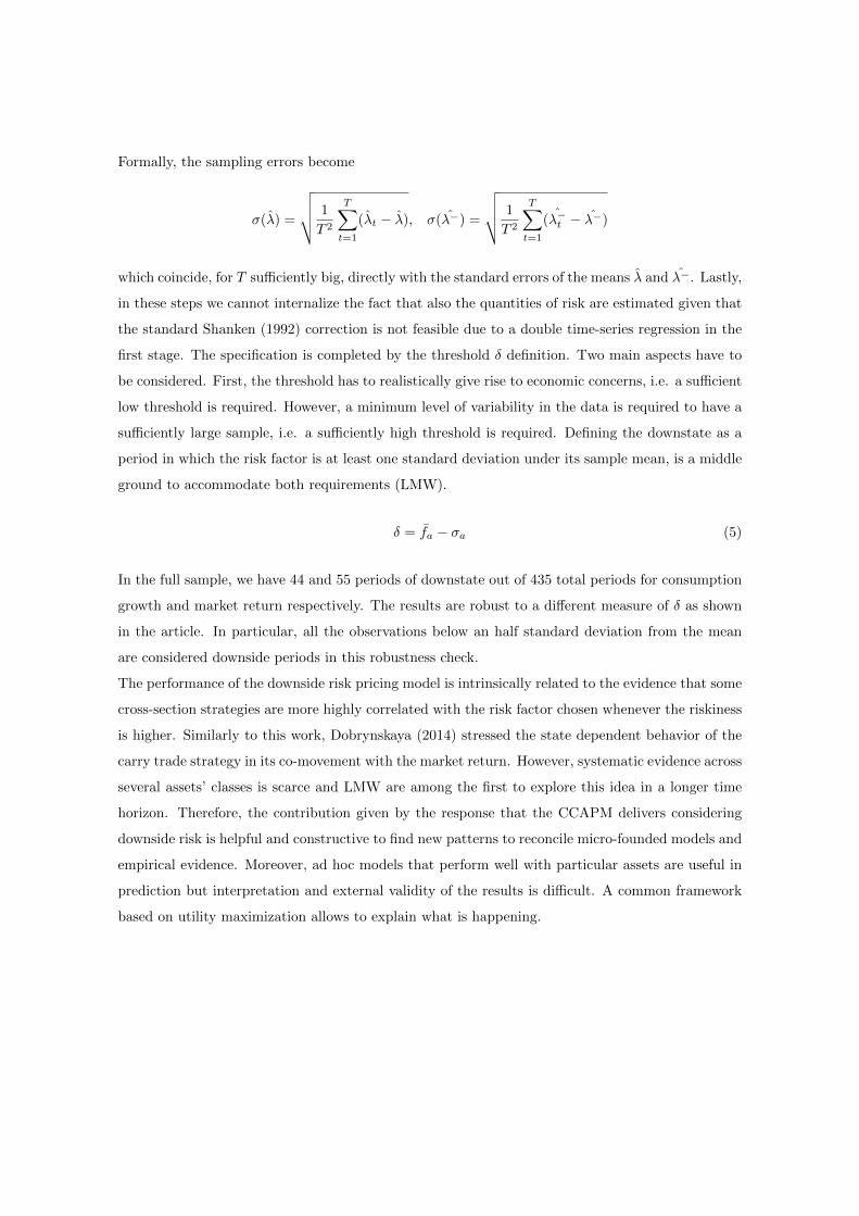
Formally, the sampling errors become

σ(λ̂) =

√√√√ 1

T 2

T∑t=1

(λ̂t − λ̂), σ(λ̂−) =

√√√√ 1

T 2

T∑t=1

(λ̂−t − λ̂−)

which coincide, for T sufficiently big, directly with the standard errors of the means λ̂ and λ̂−. Lastly,

in these steps we cannot internalize the fact that also the quantities of risk are estimated given that

the standard Shanken (1992) correction is not feasible due to a double time-series regression in the

first stage. The specification is completed by the threshold δ definition. Two main aspects have to

be considered. First, the threshold has to realistically give rise to economic concerns, i.e. a sufficient

low threshold is required. However, a minimum level of variability in the data is required to have a

sufficiently large sample, i.e. a sufficiently high threshold is required. Defining the downstate as a

period in which the risk factor is at least one standard deviation under its sample mean, is a middle

ground to accommodate both requirements (LMW).

δ = f̄a − σa (5)

In the full sample, we have 44 and 55 periods of downstate out of 435 total periods for consumption

growth and market return respectively. The results are robust to a different measure of δ as shown

in the article. In particular, all the observations below an half standard deviation from the mean

are considered downside periods in this robustness check.

The performance of the downside risk pricing model is intrinsically related to the evidence that some

cross-section strategies are more highly correlated with the risk factor chosen whenever the riskiness

is higher. Similarly to this work, Dobrynskaya (2014) stressed the state dependent behavior of the

carry trade strategy in its co-movement with the market return. However, systematic evidence across

several assets’ classes is scarce and LMW are among the first to explore this idea in a longer time

horizon. Therefore, the contribution given by the response that the CCAPM delivers considering

downside risk is helpful and constructive to find new patterns to reconcile micro-founded models and

empirical evidence. Moreover, ad hoc models that perform well with particular assets are useful in

prediction but interpretation and external validity of the results is difficult. A common framework

based on utility maximization allows to explain what is happening.

Data

The dataset for this article is retrieved from multiple public available data. The monthly U.S.

consumption data is obtained from the ’National Income and Product Accounts of the United

States’ (NIPA tables), the population level from the ’Current Population Survey’, both collected by

the U.S. Bureau of Economic Analysis and downloaded through the FRED, Federal Reserve Bank of

St. Louis portal. The monthly excess returns for currencies, equity, and commodities are obtained

from the journal website where LMW uploaded a replicating dataset. The sample period stars in

January 1974 and ends in March 2010 for a total of 435 observations with the exception of the

commodity returns ending in December 2008 (420 observations).

Consumption is defined as the sum of non-durable and services (PCEND1,PCES2) reducing the

measurement problem between expenditures and actual consumption, as remarked by Hall (1978).

Both time series are released at the aggregate U.S. level in billions of dollars, seasonally adjusted

annual rate. Services account for about 70% of the constructed measure of consumption. Population

used to calculate the per capita numbers is the civilian non-institutional population (CNP16OV3)

reported in thousands and defined as ”a person 16 years of age and older residing in the 50 states

and the District of Columbia, who are not inmates of institutions (e.g., penal and mental facilities,

homes for the aged), and who are not on active duty in the Armed Forces”. Throughout the analysis

consumption is interpreted with the beginning-of-period convention following Engsted and Moller

(2015) that remarks the striking difference between beginning and end of period conventions’ for

the performance of CAPM. Basically, the consumption reported on national account for a particular

month is interpreted as the flow occurred the period before.

The market return is the value-weighted Center for Research in Security Prices (CRSP) US equity

market log excess return. The use of this broad definition of market is common in the literature and

conservative in avoiding automatic increase in the correlation with the non-equity test assets and

the market risk factor.

Equity returns are based on the six Fama and French portfolios sorted on size and book-to-

market publicly available on Kenneth French Website4. The currencies returns covering 53 countries

1U.S. Bureau of Economic Analysis, Personal Consumption Expenditures: Nondurable Goods [PCEND], retrievedfrom FRED, Federal Reserve Bank of St. Louis; https://fred.stlouisfed.org/series/PCEND

2U.S. Bureau of Economic Analysis, Personal Consumption Expenditures: Services [PCES], retrieved from FRED,Federal Reserve Bank of St. Louis; https://fred.stlouisfed.org/series/PCES

3U.S. Bureau of Labor Statistics, Population Level [CNP16OV], retrieved from FRED, Federal Reserve Bank ofSt. Louis; https://fred.stlouisfed.org/series/CNP16OV

4http://mba.tuck.dartmouth.edu/pages/faculty/ken.french/datalibrary.html

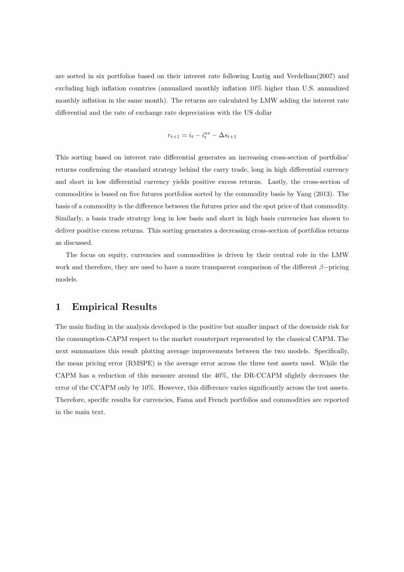
are sorted in six portfolios based on their interest rate following Lustig and Verdelhan(2007) and

excluding high inflation countries (annualized monthly inflation 10% higher than U.S. annualized

monthly inflation in the same month). The returns are calculated by LMW adding the interest rate

differential and the rate of exchange rate depreciation with the US dollar

rt+1 = it − iust −∆st+1

This sorting based on interest rate differential generates an increasing cross-section of portfolios’

returns confirming the standard strategy behind the carry trade, long in high differential currency

and short in low differential currency yields positive excess returns. Lastly, the cross-section of

commodities is based on five futures portfolios sorted by the commodity basis by Yang (2013). The

basis of a commodity is the difference between the futures price and the spot price of that commodity.

Similarly, a basis trade strategy long in low basis and short in high basis currencies has shown to

deliver positive excess returns. This sorting generates a decreasing cross-section of portfolios returns

as discussed.

The focus on equity, currencies and commodities is driven by their central role in the LMW

work and therefore, they are used to have a more transparent comparison of the different β−pricing

models.

1 Empirical Results

The main finding in the analysis developed is the positive but smaller impact of the downside risk for

the consumption-CAPM respect to the market counterpart represented by the classical CAPM. The

next summarizes this result plotting average improvements between the two models. Specifically,

the mean pricing error (RMSPE) is the average error across the three test assets used. While the

CAPM has a reduction of this measure around the 40%, the DR-CCAPM slightly decreases the

error of the CCAPM only by 10%. However, this difference varies significantly across the test assets.

Therefore, specific results for currencies, Fama and French portfolios and commodities are reported

in the main text.

Average ImprovementsOutlined are the average improvements for two β-pricing model with an additional downside risk specification for both.

The performance is based on the root squared pricing error (RMSPE) that is averaged out across equity, currency

and commodities portfolios. The sample period of these test assets is January 1974 to March 2010 for a total of 435

observations for the equity and currency assets and January 1974 to December 2008 for the commodity assets for a

total of 420 observations.

Conclusion

The economic literature has always stressed how reconciling micro-founded models with empirical

evidence is at the core of the current research (Cochrane 2011). However, the field is still expanding

and research is ongoing. Using the methodology constructed by LMW, this article analyzes the

impact of conditional risk on the classical consumption-CAPM of Lucas (1978) and Breeden (1979).

Indeed, the downside risk is strictly connected to the high marginal utility of investors in distressed

periods. The asymmetry in covariance in good and bad times is a powerful tool to construct an

asset pricing model that captures relevant differences in risk.

Results depict a clear message. The conditional risk has a positive and significant impact on the

performance of the classical linear models (CAPM and CCAPM) but, the improvement is greater

for the market factor case when single asset classes are analyzed. In particular, against an average

improvement of 40% for the CAPM, the CCAPM presents a smaller gain of a one fourth magnitude.

Moreover, the striking difference emerges when the downside risk model for the consumption factor

is tested against the cross-section of test assets. Indeed, while the CAPM is able to price the cross-

section with the inclusion of the conditional risk, this is not the case for the consumption based

model. Further research is still required as highlighted by the behavior of the selected models under

different sample periods. In fact, as the conditional risk seems to generally over-predict returns in

distressed times represented by the 2008 Sub-prime crisis, focusing on consumer industry shows that

the Covid19 crisis seems to reduce the gap when the consumption based model with the inclusion

of conditional risk is considered.

To conclude this discussion a last comment is required. The econometric framework specified

delivers to the researcher an important level of flexibility given the exogenous parametrization of

the downside threshold and allows to gain some insights in the asset pricing literature having still

a preference based framework at its core. However, an attempt to internalize in the model the

downside periods threshold could be pivotal for a correct understanding of the mechanism behind

the investors investment decisions, a challenge that does not age despite is long tradition and that

continues to inspire economists in their efforts.