Embed Size (px)
Citation preview
CONSERVATIVITY OF COERCIVE SUBTYPING
TAO XUE, ZHAOHUI LUO, AND ROBIN ADAMS
Department of Computer Science, Royal Holloway, University of Londone-mail address: taoxue, zhaohui, robin @cs.rhul.ac.uk
Abstract. Coercive subtyping provides an abbreviation mechanism, which offers a simplebut powerful approach to the study of subtyping in type theories with canonical objects.In this paper we give an adequate formulation of coercive subtyping that extends typetheories such as Martin-lof’s type theory and UTT and prove that it is a coservativeextension.
1. Introduction
We often wish to introduce a notion of subtyping into type theory, analogous to thesubset relation in set theory. Ceocive subtyping [Luo97] is one way to introduce such anotion into the type theories formulated in the logical framework LF[Luo94], a Church-typed version of Martin-Lof’s Logical framework [NPS90]. The basic idea is that, giventwo different types A and B, we can make A into a subtype of B by declaring a functionc : (A)B to be a coercion, meaning we identify any object a : A with the object c(a) : B.
Since type theories have been implemented in proof assistants, like Coq, Plastic, Adga,coercive subtyping has been implemented by Saibi in Coq[Sai97] and Callaghan in plastic[CL01].
In the formal system of coercive subtyping, we distinguish basic and derived coercions.The system of basic coercions is open in the sense that new coercions may be declared, andthe derived coercions are those could be derived with the rules in the type system fromthe basic coercions. There are different ways of introducing the basic coercions and extendtype theories with coercive subtyping. In [Luo99], the system of basic coercions is a set Rof rules whose conclusions are subtyping judgements of form Γ ⊢ A <c B : Type, like:
Γ ⊢ A <c B : Type
Γ ⊢ List(A) <map(c) List(B) : Type
The basic coercions are require to be coherent (any two coercions of the same domainare required to be equal). With R and original type system T , we could construct a typesystem T [R]. In [LL05], a set C is used for basic coercions. C is a well-defined set of coercion
LOGICAL METHODSIN COMPUTER SCIENCE DOI:10.2168/LMCS-???
c⃝Creative Commons
1
2
judgements, which satisfy congruence, transitivity, substitution, coherence and weakening.For an informal example, C should be a set like:
{Γ ⊢ A <c1 B, Γ ⊢ B <c1 C, Γ ⊢ A <c2◦c1 C, ...}with type system T , we can generate a system T [C].
Unfortunately, we find the extension system T [R](whose basic coercions are coercionrules) is not quite the right formulation for coercive subtyping. More precisely, we form acounter example to show that T [R] is not a conservative extension over T in section 3.2.
Conservativity is one of the most important properties we want to consider, whenwe make an extension of a type system. Informally, conservativity means that all thosejudgements which can be derived in the extension system, can be derived in the originalsystem as well. Intuitively, it implies that the extension has no more power than the originalsystem. Since we think coercive subtyping is just an abbreviation mechanism which shouldnot increase the power of the system, we want the conservativity property to hold.
We believe T [C](whose basic coercions are coercion judgements) is a more general ap-proach for coercive subtyping. Even when we have a set of basic coercions with the form ofrules, we could use it to generate a set of basic coercions with the form of only judgements.There was a proof which showed T [R] is a conservative extension over T [SL02]. Althoughthe result is not right, the methods in the proof light us a way to prove that T [C] is aconservativity extension of over T .
In this paper, we will give an informal description of ceorcive subtyping and the formaldefinition of T [C] in section2. Section 3 discusses coherence and conservativity, gives ainformal description on the conservativity proof. Section 4.3 proves the conservativity ofT [C] over T . In section ??, we discuss the conservativity problem of T [R], show a counterexample, and discuss the relationship between T [C] and T [R].
2. Background
2.1. Specifying type theories in LF.
In this paper, we consider the type theory UTT specified in LF to be our basic typesystem T . Here, we briefly explain what LF is and how UTT and other type theories canbe specified in LF, further details can be found in [Luo94].
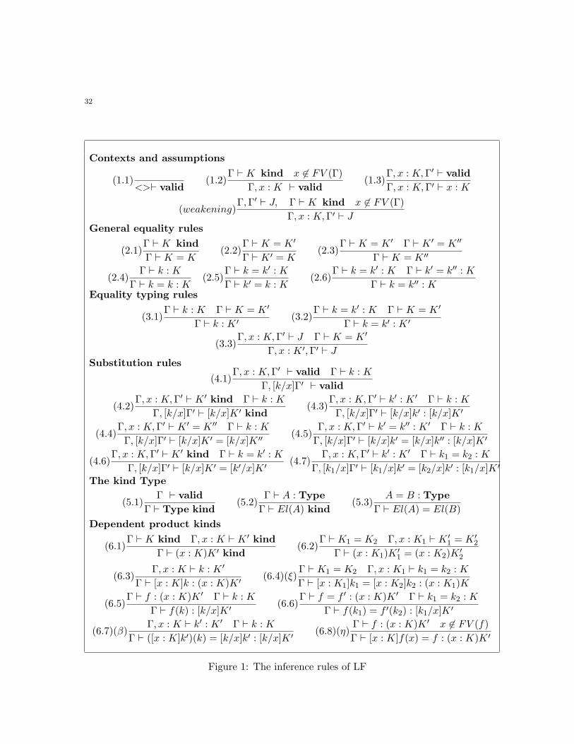
2.1.1. The logical framework LF.LF[Luo94], whose rules are given in Appendix A(slightly different from the rules in [Luo94]),is a logical framework, which can be used as a meta-language to specify type theories. LFis a simple type system with terms of the following forms:
Type, El(A), (x : K)K ′, [x : K]k′, f(k)
The kind Type represents the conceptual universe of type, El(A) represents the kind ofobject of A, (x : K)K ′ represents dependent product, [x : K]k′ represents abstraction, andf(k) is for application.
Notation 2.1. We shall use the following notations:
• We often write (K)K’ instead of (x:K)K’ if x does not occur free in K.• We write A for El(A) and (A)B for (El(A))El(B) when no confusion may occur.
3
• Substitution: [N/x]M stands for the expression obtained from M by substituting Nfor the free occurrences of variable x in M , defined as usual with possible changes ofbound variables; informally we sometimes use M [x] to indicate that variable x mayoccur free in M and subsequently write M [N ] for [N/x]M , when no confusion mayoccur.
• Function composition: for f : (K1)K2 and g : (K2)K3, we define
g ◦ f =df [x : K1]g(f(x)) : (K1)K3
• We write Γd⊢J , if d is a derivation with final judgement Γ ⊢ J .
LF could be used to specify type theories, such as Martin-Lof’s type theory [NPS90]and UTT [Luo94]. In general, a specification of a type theory in LF consists of a collectionof new constants and new computation rules. Formally, declaring a new constant k of kindK by writing
k : K
is to introduce the following inference rule:
Γ ⊢ valid
Γ ⊢ k : Kand asserting computation rule by writing
k = k′ : K where ki : Ki(i = 1, ..., n)
is to introduce the following equality inference rule:
Γ ⊢ ki : Ki(i = 1, ..., n) Γ ⊢ k : K Γ ⊢ k′ : K
Γ ⊢ k = k′ : K
2.1.2. The formulation of UTT.UTT is a type theory consists of a impredicative universe of logical propositions, a largeclass of inductive data types, and predicate universes. Taking inductive data type N fornatural number as example, we could specify N in LF as followed . Rules for other datatypes, internal logic and predicate universes are similar, further details could be found inChapter9 of [Luo94].
For the type N of natural numbers, we have the following constants
N : Type0 : N
succ : (N)NRecN : (C : (N)Type)(c : C(0))(f : (x : N)(C(x))C(succ(x)))(n : N)C(n)
and computation rule:
RecN (C, c, f, 0) = c : C(0)
RecN (C, c, f, succ(n)) = f(n,RecN (C, c, f, n)) : C(succ(n))
So, the inference rules are:
4
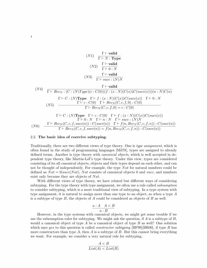
(N1)Γ ⊢ valid
Γ ⊢ N : Type
(N2)Γ ⊢ valid
Γ ⊢ 0 : N
(N3)Γ ⊢ valid
Γ ⊢ succ : (N)N
(N4)Γ ⊢ valid
Γ ⊢ RecN : (C : (N)Type)(c : C(0))(f : (x : N)(C(x))C(succ(x)))(n : N)C(n)
(N5)
Γ ⊢ C : (N)Type Γ ⊢ f : (x : N)(C(x))C(succ(x)) Γ ⊢ 0 : NΓ ⊢ c : C(0) Γ ⊢ RecN (C, c, f, 0) : C(0)
Γ ⊢ RecN (C, c, f, 0) = c : C(0)
(N6)
Γ ⊢ C : (N)Type Γ ⊢ c : C(0) Γ ⊢ f : (x : N)(C(x))C(succ(x))Γ ⊢ 0 : N Γ ⊢ n : N Γ ⊢ succ : (N)N
Γ ⊢ RecN (C, c, f, succ(n)) : C(succ(n)) Γ ⊢ f(n,RecN (C, c, f, n)) : C(succ(n))
Γ ⊢ RecN (C, c, f, succ(n)) = f(n,RecN (C, c, f, n)) : C(succ(n))
2.2. The basic idea of coercive subtyping.
Traditionally, there are two different views of type theory. One is type assignment, which isoften found in the study of programming languages [Mil78], types are assigned to alreadydefined terms. Another is type theory with canonical objects, which is well accepted in de-pendent type theory, like Martin-Lof’s type theory. Under this view, types are consideredconsisting of its all canonical objects, objects and their types depend on each other, and cannot be thought of independently. For example, the type Nat for natural numbers could bedefined as Nat = 0|succ(Nat), Nat consists of canonical objects 0 and succ, and numbersexist only because they are objects of Nat.
With different views of type theory, we have related but different ways of consideringsubtyping. For the type theory with type assignment, we often use a rule called subsumptionto consider subtyping, which is a more traditional view of subtyping. In a type system withtype assignment, it is natural to assign more than one type to an object, so when a type Ais a subtype of type B, the objects of A could be considered as objects of B as well.
a : A A < B
a : BHowever, in the type systems with canonical objects, we might get some trouble if we
use the subsumption rules for subtyping. We might ask the question, if A is a subtype of B,would a canonical object of type A be a canonical object of type B as well? One solutionwhich says yes to this question is called constructor subtyping [BF99][BR00], if type B hasmore constructors than type A, then A is a subtype of B. But this cannot bring everythingwe want. For example, we consider a very natural rule for subtyping,
A < B
List(A) < List(B)
5
where List(M) has constructors nil(M) and consM , for any type M . Now List(A) consistsof canonical objects nil(A) and consA, List(B) consists of canonical objects nil(B) andconsB. But now we are not quite clear whether nil(A) should be a canonical object ofList(B) or not.
Coercive subtyping[Luo99] is an alternative approach to introduce subtyping into typesystems with canonical objects, which can avoid the problem above. The basic idea is thatwhen we consider A as a subtype of B, we make a unique coercion c from A to B, where cis a special function from A to B, written as A <c B. The coercion actually plays a role asan abbreviation. More precisely, if f is a function from B to C, then f could apply on anyobject a of type A, f(a) is of type C and definitionally equal to f(c(a)). Intuitively, whenf requires an object of B, a stands for a mapping of c(a), and we could consider f(a) as anabbreviation for f(c(a)).
Remark 2.2. Unlike the traditional view of subtyping with subsumption rule, the objectsof subtypes do not obtain more types in coercive subtyping. The object a is an object oftype A not an object of type B. The coercion will be applied only when a function f isapplied on a. Although f(a) is now a well-typed term of type C, it is just an abbreviationfor f(c(a)), which is already of type C.
Example 2.3. With coercive subtyping, we could think example above in this way
A <c B
List(A) <map(A,B,c) List(B)
where map(A,B, c) is a function from List(A) to List(B) such that map(A,B, c)(nil(A)) =nil(B) and map(A,B, c)(cons(A, a, l)) = cons(B, c(a),map(A,B, c)(l)).
We can take another example, to see how coercive subtyping could be used in type-theoretical semantics in linguistic interpretation[Luo10].
Example 2.4. If we want to interpret John runs. As common sense, we could assume
[[runs]] : Human → Prop [[John]] : Man
but we cannot apply [[runs]] on [[John]] now. If we define coercion c from Man to Human,
Man <c Human
which means Man is a subtype of Human, we could naturally consider [[John]] is an objectof Human via c, hence John runs could be interpreted as
([[runs]])[[John]] : Prop
3. Coercive sutyping: an adequate formulation
The way we generate a type theory with coercive subtyping, is to extend an exsited typetheory with coercive judgement follwing some rules. When we make an extension of onesystem, conservativity is one of the most important properties we want to consider of.
Definition 3.1. (conservative extension)Given two systems T1, T2 and T2 is an extensionof T1. We call T2 is a conservative extension of T1, if everything in the language of T1 thatcan be derived T2, can be derive in T1 as well.
6
Intuitively, T2 does not have more power than T1. This is our view of coercive subtyping.We think coercions are just a mechanism of abbreviation, so it should not increase any powerof the original type system. Therefore extending a type theory, with coercive subtypingshould produce a conservative extension.
3.1. Coherence.
Informally, coherence in coercive subtyping means that for two types with subtyping re-lation, there is a unique coercion between them. It is very closely related to conservativity.Suppose in a system with coercive subtyping, c is a coercion from K0 to K1,
Γ ⊢ K0 <c K1, Γ ⊢ k : K0, and Γ ⊢ f : (x : K1)K2
Using coercion definition rule, we have
Γ ⊢ f(c(k)) = f(k) : [ck/x]K2
If there is another coercion c′ which is from K0 to K1 as well, Γ ⊢ c = c′ : (K0)K1, we canget
Γ ⊢ f(c′(k)) = f(k) : [c′k/x]K2
Since f is arbitrary, we take f ≡ [x : K1]x and f : (x : K1)K1. x is not free in K1, bydefinition, [ck/x]K1 ≡ [c′k/x]K1 ≡ K1, so
Γ ⊢ f(c(k)) = f(k) : K1 Γ ⊢ f(c′(k)) = f(k) : K1
Now we haveΓ ⊢ f(c(k)) = f(c′(k)) : K1
we can choose f ≡ [x : K1]x, hence
Γ ⊢ c(k) = c′(k) : K1
choose k to be variable y : K1 ,
Γ, y : K0 ⊢ c(y) = c′(y) : K1
Γ ⊢ [y : K0]c(y) = [y : K0]c′(y) : (K0)K1
and by the η ruleΓ ⊢ c = c′ : (K0)K1
In this case, the extension is not conservative. So coherence must hold in the type systemwith coercive subtyping.
3.2. Problem of exsiting formulation.
In [Luo97][Luo99], when coercive subtyping was first introduced in LF, the basic coer-cions were given by a set of coherent rules R, whose conclusions were coercive subtypingjudgements. Extending T with R and other rules, we obtain a type system T [R] withcoercive subtyping. System T [R] was proved to be a conservative extension over systemT in [SL02]. However,the proof was found to be incorrect, and for some R, T [R] is not aconservative extension over T . Informally, the problem is that we can use the judgementgenerated by coercive application back on the rules in R. In this way, some rules whosepremises are not well-typed and who will never be used in T may be used now. These rulesmight contain some coercive subtyping judgements which might voilate the coherence asconclusion. More precisely, let’s see the following counter example.
7
Example 3.2. Suppose Nat : Type, Bool : Type, c1 : (Nat)Bool, c2 : (Nat)Bool,∀x : Nat.c1(x) = true, c2(x) = false and idb ≡ [x : Bool]x. The following two rules are inthe set R
Γ ⊢ valid
Γ ⊢ Nat <c1 Bool : Type(∗)
Γ ⊢ n : Nat Γ ⊢ g : (Bool)Bool Γ ⊢ g(n) : Bool
Γ ⊢ Nat <c2 Bool : Type(∗∗)
Although there are two different coercions from Nat to Bool, R is still coherent. Thereason is, in rule (**), g is of type (Bool)Bool and a is of type Nat, since we haven’tintroduced coercion application rule in T [R]0, so g(a) : Bool is not well typed in T [R]0.So the second rule will never be used in T [R]0, and we have only one coercive subtypingrelation from Nat to Bool.
But in system T [R], after introducing coercive application rule, we have.
Γ ⊢ g : (Bool)Bool Γ ⊢ n : NatΓ ⊢ Nat :<c1 Bool : Type
Γ ⊢ Nat <c1 Bool
Γ ⊢ g(a) : Bool
Now, rule(**) can be applied, and we get another coercive subtyping c2 from Nat toBool. Using two coercion subtyping judgments in coercive definition rule separately,
Γ ⊢ idb : (Bool)Bool Γ ⊢ 0 : NatΓ ⊢ Nat <c1 Bool : Type
Γ ⊢ Nat <c1 Bool
Γ ⊢ idb(0) = idb(c1(0)) : Bool
Γ ⊢ idb : (Bool)Bool Γ ⊢ 0 : NatΓ ⊢ Nat <c2 Bool : Type
Γ ⊢ Nat <c2 Bool
Γ ⊢ idb(0) = idb(c2(0)) : Bool
idb(c1(0)) = c1(0) : Bool, idb(c2(0)) = c2(0) : Bool, so in T [R] we have
Γ ⊢ c1(0) = c2(0) : Bool
But in T , as the definition shows c1(0) = true, c2(0) = false,
Γ ⊢ c1(0) = c2(0) : Bool
It’s nonconservative, somehow inconsistent.
3.3. A formal presentation of system T [C].
System T [C] is another way to extend type theory T specified in LF with coercive su-typing, C is a set of preset coercive judgements. In T [C], the judgements generated bycoercive application can not affect the judgements in C. The above problem in T [R] wouldnot occur in T [C], and coherence is held. So we are wondering whether T [C] is a conservativeextension over T , and prove it in this paper. The formal presentation of T [C] is followed,further details could be found in [LL05][Luo05].
Definition 3.3. (Well-defined coercions) If C is a set of subtyping judgements of the formΓ ⊢ A <c B : Type which satisfies the following conditions, we say that C is a well-definedset of judgement for coercions, or briefly called Well-Defined Coercions(WDC).
8
(1) (Coherence)(a) Γ ⊢ A <c B : Type ∈ C, implies Γ ⊢ A : Type, Γ ⊢ B : Type, Γ ⊢ c : (A)B.(b) Γ ⊢ A <c A : Type ∈ C, for any Γ, A, Γ, c.(c) Γ ⊢ A <c1 B : Type ∈ C and Γ ⊢ A <c2 B : Type ∈ C, imply Γ ⊢ c1 = c2 :
(A)B.(2) (Congruence)Γ ⊢ A <c B : Type ∈ C, Γ ⊢ A = A′ : Type, Γ ⊢ B = B′ : Type and
Γ ⊢ c = c′ : (A)B, imply Γ ⊢ A′ <′c B
′ : Type ∈ C.(3) (Transitivity) Γ ⊢ A <c1 B : Type ∈ C and Γ ⊢ B <c2 A′ : Type ∈ C, imply
Γ ⊢ A < c2 ◦ c1A′ : Type ∈ C.(4) (Substitution) Γ, x : K,Γ′ ⊢ A <c B : Type ∈ C implies Γ, [k/x]Γ′ ⊢ [k/x]A <[k/x]c
[k/x]B : Type ∈ C, for any k such that Γ ⊢ k : K(5) (Weakening) Γ,Γ′ ⊢ A <c B : Type ∈ C, Γ ⊢ K kind and x ∈ FV (Γ)
∪FV (Γ′)
imply Γ, x : K,Γ′ ⊢ A <c B : Type ∈ C
3.3.1. The system T [C]0.T [C]0 is an extension of system T with coercive judgments of form A <c B : Type and thefollowing rules
• A well-defined set of judgments for coercions (WDC) C,• coercion inference rule
(ST1)Γ ⊢ A <c B : Type ∈ CΓ ⊢ A <c B : Type
• congruence rule
(ST2)Γ ⊢ A <c B : Type Γ ⊢ A = A′ : Type Γ ⊢ B′ : Type Γ ⊢ c = c′ : (A)B
Γ ⊢ A′ <c′ B′ : Type
• transitivity rule
(ST3)Γ ⊢ A <c B : Type Γ ⊢ B <c′ C : Type
Γ ⊢ A <c◦c′ C : Type
• substitution rule
(ST4)Γ, x : K,Γ′ ⊢ A <c B : Type Γ ⊢ k : K
Γ, [k/x]Γ′ ⊢ [k/x]A <[k/x]c [k/x]B : Type
3.3.2. The system T [C]0K .System T [C]0K is obtained from T [C]0 by adding the new subkinding judgement of formΓ ⊢ K <c K
′ and the following subkinding inference rules
• Basic subkinding rule
(SK1)Γ ⊢ A <c B : Type
Γ ⊢ El(A) <c El(B)
• Subkinding for dependent product kinds
(SK2)Γ ⊢ K ′
1 <c1 K1 Γ, x′ : K ′1 ⊢ [c1(x
′)/x]K2 = K ′2 Γ, x : K1 ⊢ K2 : kind
Γ ⊢ (x : K1)K2 <c (x′ : K ′1)K
′2
where c ≡ [f : (x : K1)K2][x′ : K ′
1]f(c1(x′));
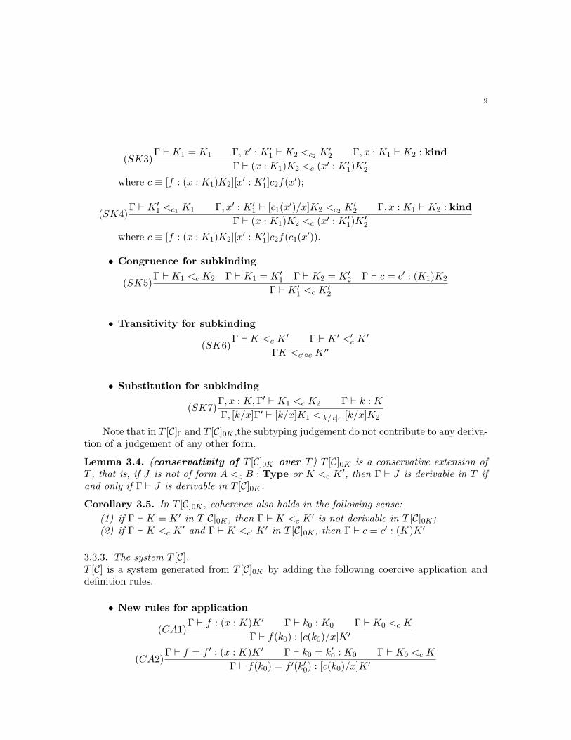
9
(SK3)Γ ⊢ K1 = K1 Γ, x′ : K ′
1 ⊢ K2 <c2 K ′2 Γ, x : K1 ⊢ K2 : kind
Γ ⊢ (x : K1)K2 <c (x′ : K ′1)K
′2
where c ≡ [f : (x : K1)K2][x′ : K ′
1]c2f(x′);
(SK4)Γ ⊢ K ′
1 <c1 K1 Γ, x′ : K ′1 ⊢ [c1(x
′)/x]K2 <c2 K ′2 Γ, x : K1 ⊢ K2 : kind
Γ ⊢ (x : K1)K2 <c (x′ : K ′1)K
′2
where c ≡ [f : (x : K1)K2][x′ : K ′
1]c2f(c1(x′)).
• Congruence for subkinding
(SK5)Γ ⊢ K1 <c K2 Γ ⊢ K1 = K ′
1 Γ ⊢ K2 = K ′2 Γ ⊢ c = c′ : (K1)K2
Γ ⊢ K ′1 <c K ′
2
• Transitivity for subkinding
(SK6)Γ ⊢ K <c K
′ Γ ⊢ K ′ <′c K
′
ΓK <c′◦c K ′′
• Substitution for subkinding
(SK7)Γ, x : K,Γ′ ⊢ K1 <c K2 Γ ⊢ k : K
Γ, [k/x]Γ′ ⊢ [k/x]K1 <[k/x]c [k/x]K2
Note that in T [C]0 and T [C]0K ,the subtyping judgement do not contribute to any deriva-tion of a judgement of any other form.
Lemma 3.4. (conservativity of T [C]0K over T ) T [C]0K is a conservative extension ofT , that is, if J is not of form A <c B : Type or K <c K
′, then Γ ⊢ J is derivable in T ifand only if Γ ⊢ J is derivable in T [C]0K .
Corollary 3.5. In T [C]0K , coherence also holds in the following sense:
(1) if Γ ⊢ K = K ′ in T [C]0K , then Γ ⊢ K <c K′ is not derivable in T [C]0K ;
(2) if Γ ⊢ K <c K′ and Γ ⊢ K <c′ K
′ in T [C]0K , then Γ ⊢ c = c′ : (K)K ′
3.3.3. The system T [C].T [C] is a system generated from T [C]0K by adding the following coercive application anddefinition rules.
• New rules for application
(CA1)Γ ⊢ f : (x : K)K ′ Γ ⊢ k0 : K0 Γ ⊢ K0 <c K
Γ ⊢ f(k0) : [c(k0)/x]K ′
(CA2)Γ ⊢ f = f ′ : (x : K)K ′ Γ ⊢ k0 = k′0 : K0 Γ ⊢ K0 <c K
Γ ⊢ f(k0) = f ′(k′0) : [c(k0)/x]K′
10
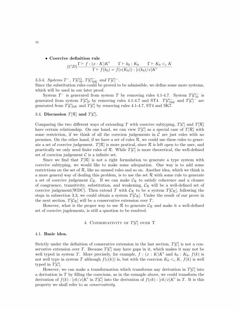
• Coercive definition rule
(CD)Γ ⊢ f : (x : K)K ′ Γ ⊢ k0 : K0 Γ ⊢ K0 <c K
Γ ⊢ f(k0) = f(c(K0)) : [c(k0)/x]K ′
3.3.4. Systems T−, T [C]10, T [C]−0K and T [C]−.
Since the substitution rules could be proved to be admissible, we define some more systems,which will be used in our later proof.
System T− is generated from system T by removing rules 4.1-4.7. System T [C]−0 isgenerated from system T [C]0 by removing rules 4.1-4.7 and ST4. T [C]−0K and T [C]− aregenerated from T [C]0K and T [C] by removing rules 4.1-4.7, ST4 and SK7.
3.4. Discussion T [R] and T [C].
Comparing the two different ways of extending T with coercive subtyping, T [C] and T [R]have certain relationship. On one hand, we can view T [C] as a special case of T [R] withsome restriction, if we think of all the coercion judgements in C are just rules with nopremises. On the other hand, if we have a set of rules R, we could use these rules to gener-ate a set of coercive judgement. T [R] is more pratical, since R is left open to the user, andpractically we only need finite rules of R. While T [C] is more theoretical, the well-definedset of coercion judgement C is a infinite set.
Since we find that T [R] is not a right formulation to generate a type system withcoercive subtyping, we would like to make some adequation. One way is to add somerestrictions on the set of R, like no unused rules and so on. Another idea, which we think isa more general way of dealing this problem, is to use the set R with some rule to generatea set of coercive judgement CR. If we can make CR to satisfy coherence and a clouserof congruence, transitivity, substitution, and weakening, CR will be a well-defined set ofcoercive judgement(WDC). Then extend T with CR to be a system T [CR], following thesteps in subsection 3.3, we could obtain a system T [CR]. Under the result of our prove inthe next section, T [CR] will be a conservative extension over T .
However, what is the proper way to use R to generate CR and make it a well-definedset of coercive jugdements, is still a question to be resolved.
4. Conservativity of T [C] over T
4.1. Basic idea.
Strictly under the definition of conserative extension in the last section, T [C] is not a con-servative extension over T . Because T [C] may have gaps in it, which makes it may not bewell typed in system T . More precisely, for example, f : (x : K)K ′ and k0 : K0, f(k) isnot well type in system T although f(c(k)) is, but with the coercion K0 <c K, f(k) is welltyped in T [C].
However, we can make a transformation which transforms any derivation in T [C] intoa derivation in T by filling the coercions, as in the exmaple above, we could transform thederivation of f(k) : [ck/x]K ′ in T [C] into the derivation of f(ck) : [ck/x]K ′ in T . It is thisproperty we shall refer to as conservativity.
11
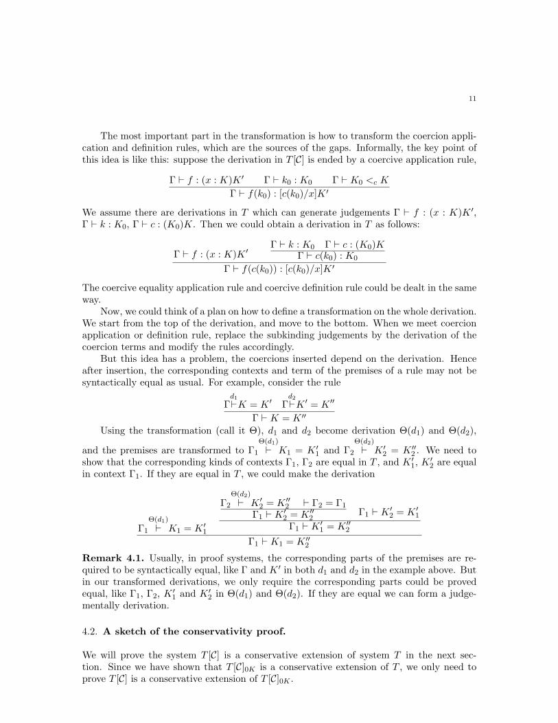
The most important part in the transformation is how to transform the coercion appli-cation and definition rules, which are the sources of the gaps. Informally, the key point ofthis idea is like this: suppose the derivation in T [C] is ended by a coercive application rule,
Γ ⊢ f : (x : K)K ′ Γ ⊢ k0 : K0 Γ ⊢ K0 <c K
Γ ⊢ f(k0) : [c(k0)/x]K ′
We assume there are derivations in T which can generate judgements Γ ⊢ f : (x : K)K ′,Γ ⊢ k : K0, Γ ⊢ c : (K0)K. Then we could obtain a derivation in T as follows:
Γ ⊢ f : (x : K)K ′Γ ⊢ k : K0 Γ ⊢ c : (K0)K
Γ ⊢ c(k0) : K0
Γ ⊢ f(c(k0)) : [c(k0)/x]K ′
The coercive equality application rule and coercive definition rule could be dealt in the sameway.
Now, we could think of a plan on how to define a transformation on the whole derivation.We start from the top of the derivation, and move to the bottom. When we meet coercionapplication or definition rule, replace the subkinding judgements by the derivation of thecoercion terms and modify the rules accordingly.
But this idea has a problem, the coercions inserted depend on the derivation. Henceafter insertion, the corresponding contexts and term of the premises of a rule may not besyntactically equal as usual. For example, consider the rule
Γd1⊢K = K ′ Γ
d2⊢K ′ = K ′′
Γ ⊢ K = K ′′
Using the transformation (call it Θ), d1 and d2 become derivation Θ(d1) and Θ(d2),
and the premises are transformed to Γ1
Θ(d1)
⊢ K1 = K ′1 and Γ2
Θ(d2)
⊢ K ′2 = K ′′
2 . We need toshow that the corresponding kinds of contexts Γ1, Γ2 are equal in T , and K ′
1, K′2 are equal
in context Γ1. If they are equal in T , we could make the derivation
Γ1
Θ(d1)
⊢ K1 = K ′1
Γ2
Θ(d2)
⊢ K ′2 = K ′′
2 ⊢ Γ2 = Γ1
Γ1 ⊢ K ′2 = K ′′
2Γ1 ⊢ K ′
2 = K ′1
Γ1 ⊢ K ′1 = K ′′
2
Γ1 ⊢ K1 = K ′′2
Remark 4.1. Usually, in proof systems, the corresponding parts of the premises are re-quired to be syntactically equal, like Γ and K ′ in both d1 and d2 in the example above. Butin our transformed derivations, we only require the corresponding parts could be provedequal, like Γ1, Γ2, K
′1 and K ′
2 in Θ(d1) and Θ(d2). If they are equal we can form a judge-mentally derivation.
4.2. A sketch of the conservativity proof.
We will prove the system T [C] is a conservative extension of system T in the next sec-tion. Since we have shown that T [C]0K is a conservative extension of T , we only need toprove T [C] is a conservative extension of T [C]0K .
12
The proof is formalize in the following way
• In subsubsection 4.3.3, a formal definition of Θ which is a transformation from T [C]−to T [C]−0K is given, some equalities are left to be proved in the rest subsections.
• The presupposition lemma and some other lemmas, which will be used to generatethe required equalities in Θ’s definition, are proved in subsubsection 4.3.4.
• In subsubsection 4.3.5, with the previous lemmas, Θ is proved to be well-defined onall the derivations of T [C]− and correct.
• Finally, in subsubsection 4.3.6, we will proof the weakening and admissibility ofsubstitution in T [C].
Remark 4.2. ************* The lemma and theorems in the following subsection areproved simultaneously.
4.3. Conservativity of T [C] over T .
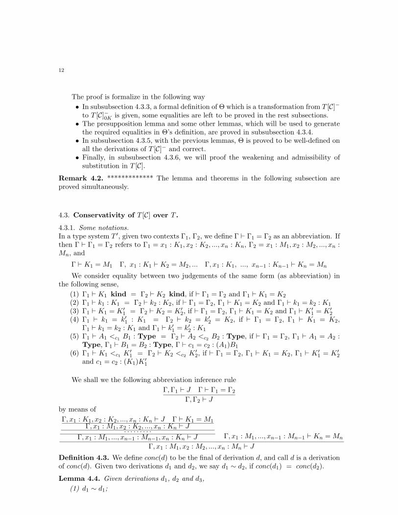
4.3.1. Some notations.In a type system T ′, given two contexts Γ1, Γ2, we define Γ ⊢ Γ1 = Γ2 as an abbreviation. Ifthen Γ ⊢ Γ1 = Γ2 refers to Γ1 = x1 : K1, x2 : K2, ..., xn : Kn, Γ2 = x1 : M1, x2 : M2, ..., xn :Mn, and
Γ ⊢ K1 = M1 Γ, x1 : K1 ⊢ K2 = M2, ... Γ, x1 : K1, ..., xn−1 : Kn−1 ⊢ Kn = Mn
We consider equality between two judgements of the same form (as abbreviation) inthe following sense,
(1) Γ1 ⊢ K1 kind = Γ2 ⊢ K2 kind, if ⊢ Γ1 = Γ2 and Γ1 ⊢ K1 = K2
(2) Γ1 ⊢ k1 : K1 = Γ2 ⊢ k2 : K2, if ⊢ Γ1 = Γ2, Γ1 ⊢ K1 = K2 and Γ1 ⊢ k1 = k2 : K1
(3) Γ1 ⊢ K1 = K ′1 = Γ2 ⊢ K2 = K ′
2, if ⊢ Γ1 = Γ2, Γ1 ⊢ K1 = K2 and Γ1 ⊢ K ′1 = K ′
2
(4) Γ1 ⊢ k1 = k′1 : K1 = Γ2 ⊢ k2 = k′2 = K2, if ⊢ Γ1 = Γ2, Γ1 ⊢ K1 = K2,Γ1 ⊢ k1 = k2 : K1 and Γ1 ⊢ k′1 = k′2 : K1
(5) Γ1 ⊢ A1 <c1 B1 : Type = Γ2 ⊢ A2 <c2 B2 : Type, if ⊢ Γ1 = Γ2, Γ1 ⊢ A1 = A2 :Type, Γ1 ⊢ B1 = B2 : Type, Γ ⊢ c1 = c2 : (A1)B1
(6) Γ1 ⊢ K1 <c1 K ′1 = Γ2 ⊢ K2 <c2 K ′
2, if ⊢ Γ1 = Γ2, Γ1 ⊢ K1 = K2, Γ1 ⊢ K ′1 = K ′
2
and c1 = c2 : (K1)K′1
We shall we the following abbreviation inference rule
Γ,Γ1 ⊢ J Γ ⊢ Γ1 = Γ2
Γ,Γ2 ⊢ J
by means of
Γ, x1 : K1, x2 : K2, ..., xn : Kn ⊢ J Γ ⊢ K1 = M1Γ, x1 : M1, x2 : K2, ..., xn : Kn ⊢ J
· · · · · · · · ·Γ, x1 : M1, ..., xn−1 : Mn−1, xn : Kn ⊢ J Γ, x1 : M1, ..., xn−1 : Mn−1 ⊢ Kn = Mn
Γ, x1 : M1, x2 : M2, ..., xn : Mn ⊢ J
Definition 4.3. We define conc(d) to be the final of derivation d, and call d is a derivationof conc(d). Given two derivations d1 and d2, we say d1 ∼ d2, if conc(d1) = conc(d2).
Lemma 4.4. Given derivations d1, d2 and d3,
(1) d1 ∼ d1;
13
(2) if d1 ∼ d2, then d2 ∼ d1;(3) if d1 ∼ d2 and d2 ∼ d3, then d1 ∼ d3.
Remark 4.5. Notice that, in any system S, we use =S for the contexts and judgmentsequality above, ∼S as well. However, if there’s no confusion may occur, we just simply use= and ∼.
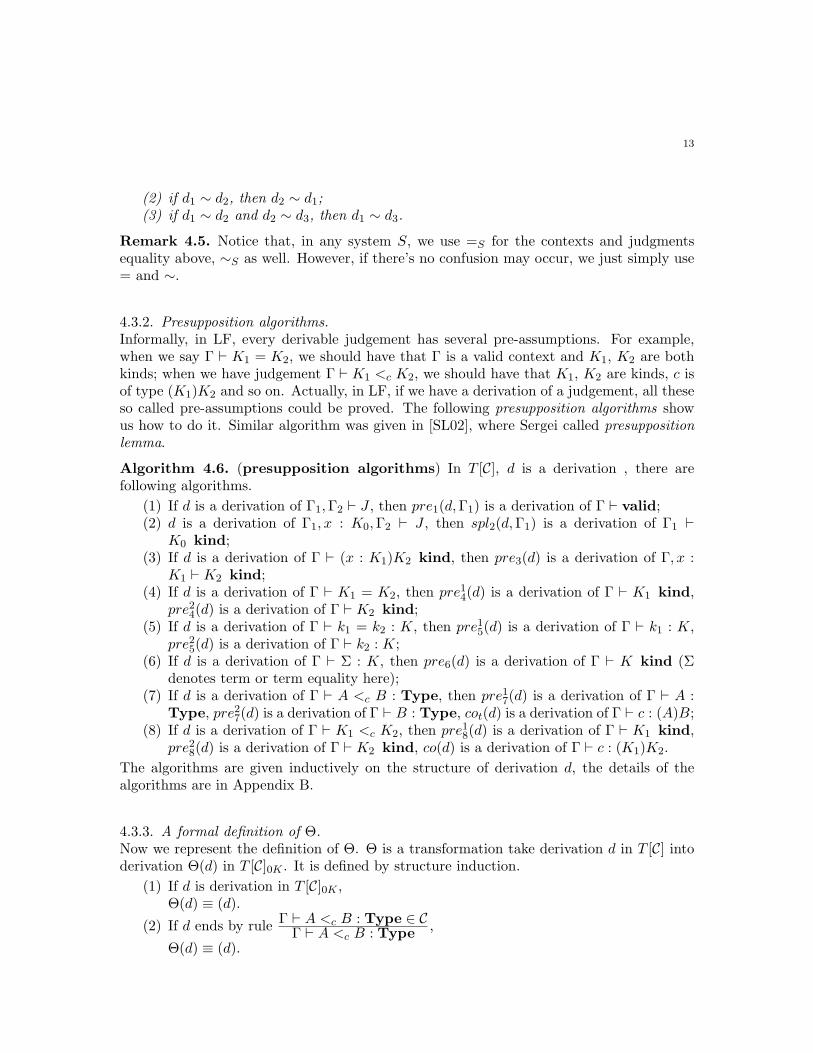
4.3.2. Presupposition algorithms.Informally, in LF, every derivable judgement has several pre-assumptions. For example,when we say Γ ⊢ K1 = K2, we should have that Γ is a valid context and K1, K2 are bothkinds; when we have judgement Γ ⊢ K1 <c K2, we should have that K1, K2 are kinds, c isof type (K1)K2 and so on. Actually, in LF, if we have a derivation of a judgement, all theseso called pre-assumptions could be proved. The following presupposition algorithms showus how to do it. Similar algorithm was given in [SL02], where Sergei called presuppositionlemma.
Algorithm 4.6. (presupposition algorithms) In T [C], d is a derivation , there arefollowing algorithms.
(1) If d is a derivation of Γ1,Γ2 ⊢ J , then pre1(d,Γ1) is a derivation of Γ ⊢ valid;(2) d is a derivation of Γ1, x : K0,Γ2 ⊢ J , then spl2(d,Γ1) is a derivation of Γ1 ⊢
K0 kind;(3) If d is a derivation of Γ ⊢ (x : K1)K2 kind, then pre3(d) is a derivation of Γ, x :
K1 ⊢ K2 kind;(4) If d is a derivation of Γ ⊢ K1 = K2, then pre14(d) is a derivation of Γ ⊢ K1 kind,
pre24(d) is a derivation of Γ ⊢ K2 kind;(5) If d is a derivation of Γ ⊢ k1 = k2 : K, then pre15(d) is a derivation of Γ ⊢ k1 : K,
pre25(d) is a derivation of Γ ⊢ k2 : K;(6) If d is a derivation of Γ ⊢ Σ : K, then pre6(d) is a derivation of Γ ⊢ K kind (Σ
denotes term or term equality here);(7) If d is a derivation of Γ ⊢ A <c B : Type, then pre17(d) is a derivation of Γ ⊢ A :
Type, pre27(d) is a derivation of Γ ⊢ B : Type, cot(d) is a derivation of Γ ⊢ c : (A)B;(8) If d is a derivation of Γ ⊢ K1 <c K2, then pre18(d) is a derivation of Γ ⊢ K1 kind,
pre28(d) is a derivation of Γ ⊢ K2 kind, co(d) is a derivation of Γ ⊢ c : (K1)K2.
The algorithms are given inductively on the structure of derivation d, the details of thealgorithms are in Appendix B.
4.3.3. A formal definition of Θ.Now we represent the definition of Θ. Θ is a transformation take derivation d in T [C] intoderivation Θ(d) in T [C]0K . It is defined by structure induction.
(1) If d is derivation in T [C]0K ,Θ(d) ≡ (d).
(2) If d ends by ruleΓ ⊢ A <c B : Type ∈ CΓ ⊢ A <c B : Type
,
Θ(d) ≡ (d).
14
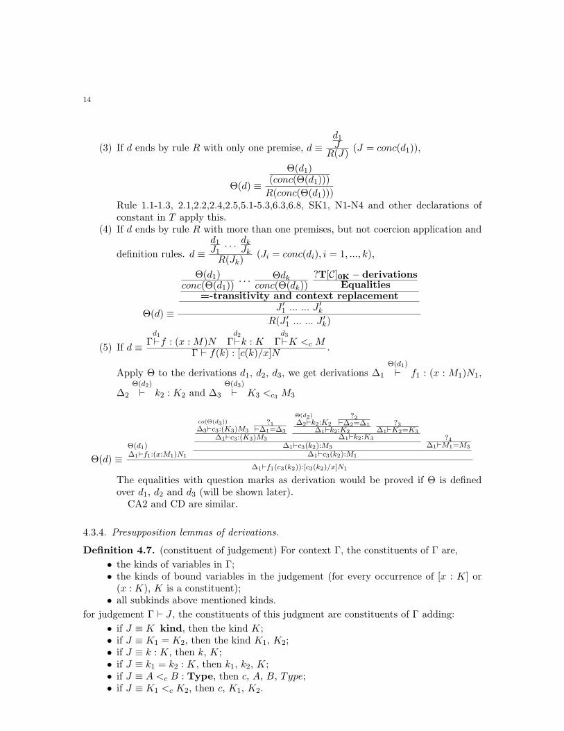
(3) If d ends by rule R with only one premise, d ≡d1J
R(J)(J = conc(d1)),
Θ(d) ≡
Θ(d1)(conc(Θ(d1)))
R(conc(Θ(d1)))Rule 1.1-1.3, 2.1,2.2,2.4,2.5,5.1-5.3,6.3,6.8, SK1, N1-N4 and other declarations ofconstant in T apply this.
(4) If d ends by rule R with more than one premises, but not coercion application and
definition rules. d ≡d1J1
. . . dkJk
R(Jk)(Ji = conc(di), i = 1, ..., k),
Θ(d) ≡
Θ(d1)conc(Θ(d1))
. . . Θdkconc(Θ(dk))
?T[C]0K − derivationsEqualities
=-transitivity and context replacementJ ′1 ... ... J ′
k
R(J ′1 ... ... J ′
k)
(5) If d ≡ Γd1⊢f : (x : M)N Γ
d2⊢k : K Γ
d3⊢K <c M
Γ ⊢ f(k) : [c(k)/x]N.
Apply Θ to the derivations d1, d2, d3, we get derivations ∆1
Θ(d1)
⊢ f1 : (x : M1)N1,
∆2
Θ(d2)
⊢ k2 : K2 and ∆3
Θ(d3)
⊢ K3 <c3 M3
Θ(d) ≡Θ(d1)∆1⊢f1:(x:M1)N1
co(Θ(d3))
∆3⊢c3:(K3)M3
?1⊢∆1=∆3
∆1⊢c3:(K3)M3
Θ(d2)
∆2⊢k2:K2
?2⊢∆2=∆1
∆1⊢k2:K2
?3∆1⊢K2=K3
∆1⊢k2:K3
∆1⊢c3(k2):M3
?4∆1⊢M1=M3
∆1⊢c3(k2):M1
∆1⊢f1(c3(k2)):[c3(k2)/x]N1
The equalities with question marks as derivation would be proved if Θ is definedover d1, d2 and d3 (will be shown later).
CA2 and CD are similar.
4.3.4. Presupposition lemmas of derivations.
Definition 4.7. (constituent of judgement) For context Γ, the constituents of Γ are,
• the kinds of variables in Γ;• the kinds of bound variables in the judgement (for every occurrence of [x : K] or(x : K), K is a constituent);
• all subkinds above mentioned kinds.
for judgement Γ ⊢ J , the constituents of this judgment are constituents of Γ adding:
• if J ≡ K kind, then the kind K;• if J ≡ K1 = K2, then the kind K1, K2;• if J ≡ k : K, then k, K;• if J ≡ k1 = k2 : K, then k1, k2, K;• if J ≡ A <c B : Type, then c, A, B, Type;• if J ≡ K1 <c K2, then c, K1, K2.
15
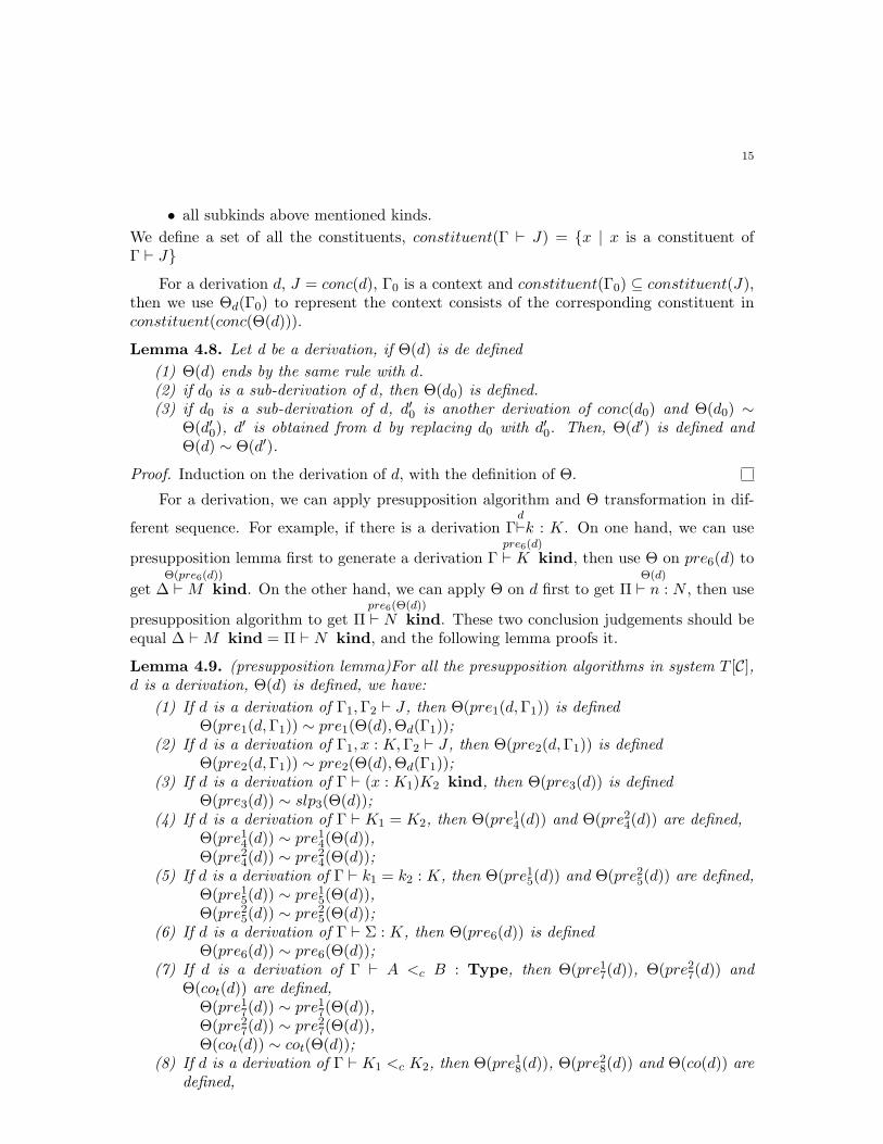
• all subkinds above mentioned kinds.
We define a set of all the constituents, constituent(Γ ⊢ J) = {x | x is a constituent ofΓ ⊢ J}
For a derivation d, J = conc(d), Γ0 is a context and constituent(Γ0) ⊆ constituent(J),then we use Θd(Γ0) to represent the context consists of the corresponding constituent inconstituent(conc(Θ(d))).
Lemma 4.8. Let d be a derivation, if Θ(d) is de defined
(1) Θ(d) ends by the same rule with d.(2) if d0 is a sub-derivation of d, then Θ(d0) is defined.(3) if d0 is a sub-derivation of d, d′0 is another derivation of conc(d0) and Θ(d0) ∼
Θ(d′0), d′ is obtained from d by replacing d0 with d′0. Then, Θ(d′) is defined andΘ(d) ∼ Θ(d′).
Proof. Induction on the derivation of d, with the definition of Θ.
For a derivation, we can apply presupposition algorithm and Θ transformation in dif-
ferent sequence. For example, if there is a derivation Γd⊢k : K. On one hand, we can use
presupposition lemma first to generate a derivationpre6(d)
Γ ⊢ K kind, then use Θ on pre6(d) to
getΘ(pre6(d))
∆ ⊢ M kind. On the other hand, we can apply Θ on d first to getΘ(d)
Π ⊢ n : N , then use
presupposition algorithm to getpre6(Θ(d))
Π ⊢ N kind. These two conclusion judgements should beequal ∆ ⊢ M kind = Π ⊢ N kind, and the following lemma proofs it.
Lemma 4.9. (presupposition lemma)For all the presupposition algorithms in system T [C],d is a derivation, Θ(d) is defined, we have:
(1) If d is a derivation of Γ1,Γ2 ⊢ J , then Θ(pre1(d,Γ1)) is definedΘ(pre1(d,Γ1)) ∼ pre1(Θ(d),Θd(Γ1));
(2) If d is a derivation of Γ1, x : K,Γ2 ⊢ J , then Θ(pre2(d,Γ1)) is definedΘ(pre2(d,Γ1)) ∼ pre2(Θ(d),Θd(Γ1));
(3) If d is a derivation of Γ ⊢ (x : K1)K2 kind, then Θ(pre3(d)) is definedΘ(pre3(d)) ∼ slp3(Θ(d));
(4) If d is a derivation of Γ ⊢ K1 = K2, then Θ(pre14(d)) and Θ(pre24(d)) are defined,Θ(pre14(d)) ∼ pre14(Θ(d)),Θ(pre24(d)) ∼ pre24(Θ(d));
(5) If d is a derivation of Γ ⊢ k1 = k2 : K, then Θ(pre15(d)) and Θ(pre25(d)) are defined,Θ(pre15(d)) ∼ pre15(Θ(d)),Θ(pre25(d)) ∼ pre25(Θ(d));
(6) If d is a derivation of Γ ⊢ Σ : K, then Θ(pre6(d)) is definedΘ(pre6(d)) ∼ pre6(Θ(d));
(7) If d is a derivation of Γ ⊢ A <c B : Type, then Θ(pre17(d)), Θ(pre27(d)) andΘ(cot(d)) are defined,
Θ(pre17(d)) ∼ pre17(Θ(d)),Θ(pre27(d)) ∼ pre27(Θ(d)),Θ(cot(d)) ∼ cot(Θ(d));
(8) If d is a derivation of Γ ⊢ K1 <c K2, then Θ(pre18(d)), Θ(pre28(d)) and Θ(co(d)) aredefined,
16
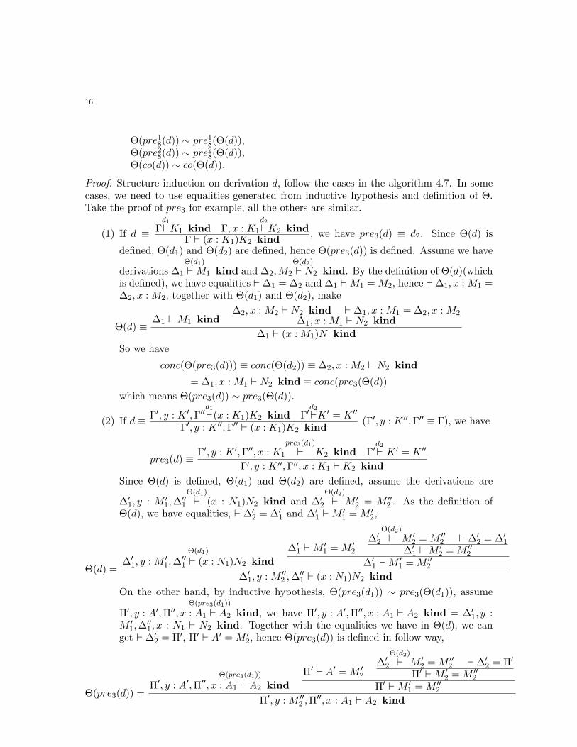
Θ(pre18(d)) ∼ pre18(Θ(d)),Θ(pre28(d)) ∼ pre28(Θ(d)),Θ(co(d)) ∼ co(Θ(d)).
Proof. Structure induction on derivation d, follow the cases in the algorithm 4.7. In somecases, we need to use equalities generated from inductive hypothesis and definition of Θ.Take the proof of pre3 for example, all the others are similar.
(1) If d ≡ Γd1⊢K1 kind Γ, x : K1
d2⊢K2 kind
Γ ⊢ (x : K1)K2 kind, we have pre3(d) ≡ d2. Since Θ(d) is
defined, Θ(d1) and Θ(d2) are defined, hence Θ(pre3(d)) is defined. Assume we have
derivationsΘ(d1)
∆1 ⊢ M1 kind andΘ(d2)
∆2,M2 ⊢ N2 kind. By the definition of Θ(d)(whichis defined), we have equalities ⊢ ∆1 = ∆2 and ∆1 ⊢ M1 = M2, hence ⊢ ∆1, x : M1 =∆2, x : M2, together with Θ(d1) and Θ(d2), make
Θ(d) ≡∆1 ⊢ M1 kind
∆2, x : M2 ⊢ N2 kind ⊢ ∆1, x : M1 = ∆2, x : M2∆1, x : M1 ⊢ N2 kind
∆1 ⊢ (x : M1)N kind
So we have
conc(Θ(pre3(d))) ≡ conc(Θ(d2)) ≡ ∆2, x : M2 ⊢ N2 kind
= ∆1, x : M1 ⊢ N2 kind ≡ conc(pre3(Θ(d))
which means Θ(pre3(d)) ∼ pre3(Θ(d)).
(2) If d ≡ Γ′, y : K ′,Γ′′d1⊢(x : K1)K2 kind Γ′d2⊢K ′ = K ′′
Γ′, y : K ′′,Γ′′ ⊢ (x : K1)K2 kind(Γ′, y : K ′′,Γ′′ ≡ Γ), we have
pre3(d) ≡Γ′, y : K ′,Γ′′, x : K1
pre3(d1)
⊢ K2 kind Γ′d2⊢ K ′ = K ′′
Γ′, y : K ′′,Γ′′, x : K1 ⊢ K2 kind
Since Θ(d) is defined, Θ(d1) and Θ(d2) are defined, assume the derivations are
∆′1, y : M ′
1,∆′′1
Θ(d1)
⊢ (x : N1)N2 kind and ∆′2
Θ(d2)
⊢ M ′2 = M ′′
2 . As the definition ofΘ(d), we have equalities, ⊢ ∆′
2 = ∆′1 and ∆′
1 ⊢ M ′1 = M ′
2,
Θ(d) =
Θ(d1)
∆′1, y : M ′
1,∆′′1 ⊢ (x : N1)N2 kind
∆′1 ⊢ M ′
1 = M ′2
∆′2
Θ(d2)
⊢ M ′2 = M ′′
2 ⊢ ∆′2 = ∆′
1
∆′1 ⊢ M ′
2 = M ′′2
∆′1 ⊢ M ′
1 = M ′′2
∆′1, y : M ′′
2 ,∆′′1 ⊢ (x : N1)N2 kind
On the other hand, by inductive hypothesis, Θ(pre3(d1)) ∼ pre3(Θ(d1)), assumeΘ(pre3(d1))
Π′, y : A′,Π′′, x : A1 ⊢ A2 kind, we have Π′, y : A′,Π′′, x : A1 ⊢ A2 kind = ∆′1, y :
M ′1,∆
′′1, x : N1 ⊢ N2 kind. Together with the equalities we have in Θ(d), we can
get ⊢ ∆′2 = Π′, Π′ ⊢ A′ = M ′
2, hence Θ(pre3(d)) is defined in follow way,
Θ(pre3(d)) =
Θ(pre3(d1))
Π′, y : A′,Π′′, x : A1 ⊢ A2 kind
Π′ ⊢ A′ = M ′2
∆′2
Θ(d2)
⊢ M ′2 = M ′′
2 ⊢ ∆′2 = Π′
Π′ ⊢ M ′2 = M ′′
2
Π′ ⊢ M ′1 = M ′′
2
Π′, y : M ′′2 ,Π
′′, x : A1 ⊢ A2 kind
17
And we get
conc(Θ(pre3(d))) ≡ Π′, y : M ′′2 ,Π
′′, x : A1 ⊢ A2 kind
= ∆′1, y : M ′′
2 ,∆′′1, x : N1 ⊢ N2 kind ≡ conc(pre3(Θ(d)))
which means Θ(pre3(d)) ∼ pre3(Θ(d)).
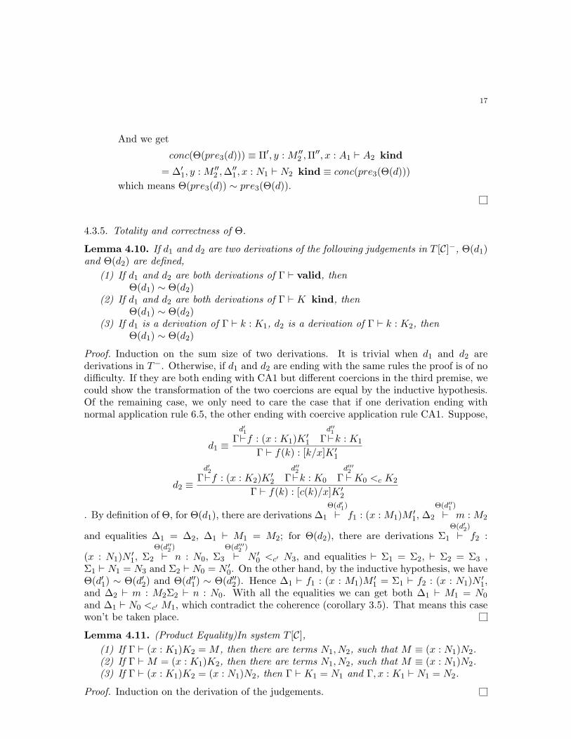
4.3.5. Totality and correctness of Θ.
Lemma 4.10. If d1 and d2 are two derivations of the following judgements in T [C]−, Θ(d1)and Θ(d2) are defined,
(1) If d1 and d2 are both derivations of Γ ⊢ valid, thenΘ(d1) ∼ Θ(d2)
(2) If d1 and d2 are both derivations of Γ ⊢ K kind, thenΘ(d1) ∼ Θ(d2)
(3) If d1 is a derivation of Γ ⊢ k : K1, d2 is a derivation of Γ ⊢ k : K2, thenΘ(d1) ∼ Θ(d2)
Proof. Induction on the sum size of two derivations. It is trivial when d1 and d2 arederivations in T−. Otherwise, if d1 and d2 are ending with the same rules the proof is of nodifficulty. If they are both ending with CA1 but different coercions in the third premise, wecould show the transformation of the two coercions are equal by the inductive hypothesis.Of the remaining case, we only need to care the case that if one derivation ending withnormal application rule 6.5, the other ending with coercive application rule CA1. Suppose,
d1 ≡Γd′1⊢f : (x : K1)K
′1 Γ
d′′1⊢k : K1
Γ ⊢ f(k) : [k/x]K ′1
d2 ≡Γd′2⊢f : (x : K2)K
′2 Γ
d′′2⊢k : K0 Γ
d′′′2⊢K0 <c K2
Γ ⊢ f(k) : [c(k)/x]K ′2
. By definition of Θ, for Θ(d1), there are derivations ∆1
Θ(d′1)
⊢ f1 : (x : M1)M′1, ∆2
Θ(d′′1 )
⊢ m : M2
and equalities ∆1 = ∆2, ∆1 ⊢ M1 = M2; for Θ(d2), there are derivations Σ1
Θ(d′2)
⊢ f2 :
(x : N1)N′1, Σ2
Θ(d′′2 )
⊢ n : N0, Σ3
Θ(d′′′2 )
⊢ N ′0 <c′ N3, and equalities ⊢ Σ1 = Σ2, ⊢ Σ2 = Σ3 ,
Σ1 ⊢ N1 = N3 and Σ2 ⊢ N0 = N ′0. On the other hand, by the inductive hypothesis, we have
Θ(d′1) ∼ Θ(d′2) and Θ(d′′1) ∼ Θ(d′′2). Hence ∆1 ⊢ f1 : (x : M1)M′1 = Σ1 ⊢ f2 : (x : N1)N
′1,
and ∆2 ⊢ m : M2Σ2 ⊢ n : N0. With all the equalities we can get both ∆1 ⊢ M1 = N0
and ∆1 ⊢ N0 <c′ M1, which contradict the coherence (corollary 3.5). That means this casewon’t be taken place.
Lemma 4.11. (Product Equality)In system T [C],(1) If Γ ⊢ (x : K1)K2 = M , then there are terms N1, N2, such that M ≡ (x : N1)N2.(2) If Γ ⊢ M = (x : K1)K2, then there are terms N1, N2, such that M ≡ (x : N1)N2.(3) If Γ ⊢ (x : K1)K2 = (x : N1)N2, then Γ ⊢ K1 = N1 and Γ, x : K1 ⊢ N1 = N2.
Proof. Induction on the derivation of the judgements.
18
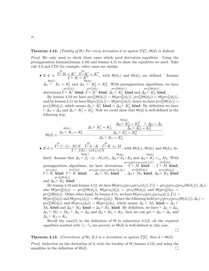
Theorem 4.12. (Totality of Θ) For every derivation d in system T [C], Θ(d) is defined.
Proof. We only need to check those cases which need derivation equalities. Using thepresupposition lemmas(lemma 4.10) and lemma 4.11 to show the equalities we need. Takerule 2.3 and CD1 for example, other cases are similar.
• If d ≡ Γd1⊢K = K ′ Γ
d2⊢K ′ = K ′′
Γ ⊢ K = K ′′ , with Θ(d1) and Θ(d2) are defined. Assume
∆1
Θ(d1)
⊢ K1 = K ′1 and ∆2
Θ(d2)
⊢ K ′2 = K ′′
2 . With presupposition algorithms, we have
derivationspre24(d1)
Γ ⊢ K ′ kind,pre14(d2)
Γ ⊢ K ′ kind,pre24(Θ(d1))
∆1 ⊢ K ′1 kind and
pre14(Θ(d2))
∆2 ⊢ K ′2 kind.
By lemma 4.10 we have pre24(Θ(d1)) ∼ Θ(pre24(d1)), pre14(Θ(d2)) ∼ Θ(pre14(d2)),
and by lemma 4.11 we have Θ(pre24(d1)) ∼ Θ(pre14(d2)), hence we have pre24(Θ(d1)) ∼
pre14(Θ(d2)), which means ∆1 ⊢ K ′1 kind = ∆2 ⊢ K ′
2 kind. By definition we have⊢ ∆1 = ∆2 and ∆1 ⊢ K ′
1 = K ′2. Now we could show that Θ(d) is well-defined in the
following way,
Θ(d) ≡
Θ(d1)
∆1 ⊢ K1 = K ′1
∆1 ⊢ K ′1 = K ′
2
Θ(d2)
∆2 ⊢ K ′2 = K ′′
2 ⊢ ∆2 = ∆1
∆1 ⊢ K ′2 = K ′′
2
∆1 ⊢ K ′1 = K ′′
2
∆1 ⊢ K1 = K ′2
• If d ≡ Γd1⊢f : (x : M)N Γ
d2⊢k : K Γ
d3⊢K <c M
Γ ⊢ f(k) : [c(k)/x]N, with Θ(d1), Θ(d2) and Θ(d3) de-
fined. Assume thatΘ(d1)
∆1 ⊢ f1 : (x : M1)N1,Θ(d2)
∆2 ⊢ k2 : K2 andΘ(d3)
∆3 ⊢ K3 <c3 M3. With
presupposition algorithms, we have derivationspre2(pre3(pre6(d1)),Γ)
Γ ⊢ M kind ,pre28(d3)
Γ ⊢ M kind,pre6(d2)
Γ ⊢ K kind,pre18(d3)
Γ ⊢ K kind,pre2(pre3(pre6(Θ(d1))),∆1)
∆1 ⊢ M1 kind ,pre28(Θ(d3))
∆3 ⊢ M3 kind,pre6(Θ(d2))
∆2 ⊢ K2 kind
andpre18(Θ(d3))
∆3 ⊢ K3 kindBy lemma 4.10 and lemma 4.12, we have Θ(pre2(pre3(pre6(d1)),Γ)) ∼ pre2(pre3(pre6(Θ(d1))),∆1),
also Θ(pre28(d3)) ∼ pre28(Θ(d3)), Θ(pre6(d2)) ∼ pre6(Θ(d2)) and Θ(pre18(d3) ∼pre18(Θ(d3)). Other other hand, by lemma 4.11, we have Θ(pre2(pre3(pre6(d1)),Γ)) ∼Θ(pre28(d3)) and Θ(pre6(d2)) ∼ Θ(pre18(d3). Hence the following hold pre2(pre3(pre6(Θ(d1))),∆1) ∼pre28(Θ(d3)) and Θ(pre6(d2)) ∼ Θ(pre18(d3), which means ∆1 ⊢ M1 kind = ∆3 ⊢M3 kind and ∆2 ⊢ K2 kind = ∆3 ⊢ K3 kind. By definition, we have ⊢ ∆1 = ∆3,∆1 ⊢ M1 = M3, ⊢ ∆2 = ∆3 and ∆2 ⊢ K2 = K3, then we can get ⊢ ∆2 = ∆1 and∆1 ⊢ K2 = K3.
Recall the case(5) in the definition of Θ in subsection 4.3.3, all the requiredequalities marked with ?1−?4 are proved, so Θ(d) is well-defined in this case.
Theorem 4.13. (Correctness of Θ) If d is a derivation in system T [C], then d ∼ Θ(d).
Proof. Induction on the derivation of d, with the totality of Θ (lemma 4.13) and using theequalities in the definition of Θ(d).
19
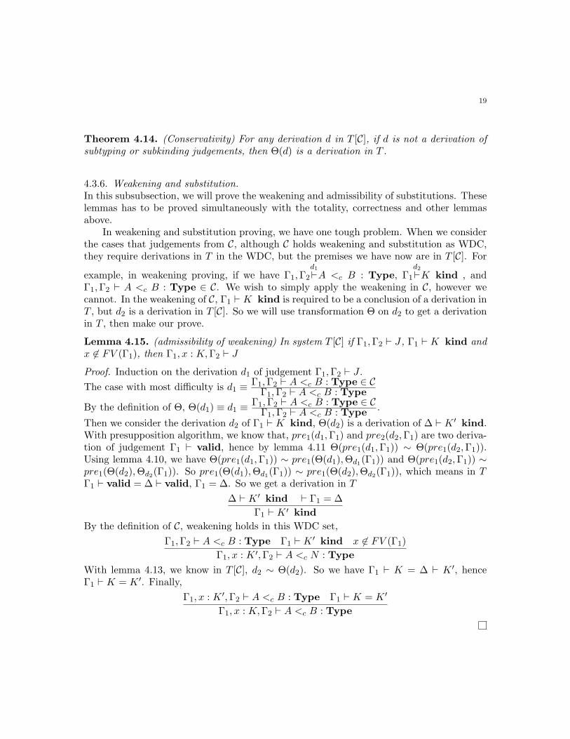
Theorem 4.14. (Conservativity) For any derivation d in T [C], if d is not a derivation ofsubtyping or subkinding judgements, then Θ(d) is a derivation in T .
4.3.6. Weakening and substitution.In this subsubsection, we will prove the weakening and admissibility of substitutions. Theselemmas has to be proved simultaneously with the totality, correctness and other lemmasabove.
In weakening and substitution proving, we have one tough problem. When we considerthe cases that judgements from C, although C holds weakening and substitution as WDC,they require derivations in T in the WDC, but the premises we have now are in T [C]. For
example, in weakening proving, if we have Γ1,Γ2
d1⊢A <c B : Type, Γ1
d2⊢K kind , and
Γ1,Γ2 ⊢ A <c B : Type ∈ C. We wish to simply apply the weakening in C, however wecannot. In the weakening of C, Γ1 ⊢ K kind is required to be a conclusion of a derivation inT , but d2 is a derivation in T [C]. So we will use transformation Θ on d2 to get a derivationin T , then make our prove.
Lemma 4.15. (admissibility of weakening) In system T [C] if Γ1,Γ2 ⊢ J , Γ1 ⊢ K kind andx ∈ FV (Γ1), then Γ1, x : K,Γ2 ⊢ J
Proof. Induction on the derivation d1 of judgement Γ1,Γ2 ⊢ J .
The case with most difficulty is d1 ≡ Γ1,Γ2 ⊢ A <c B : Type ∈ CΓ1,Γ2 ⊢ A <c B : Type
By the definition of Θ, Θ(d1) ≡ d1 ≡ Γ1,Γ2 ⊢ A <c B : Type ∈ CΓ1,Γ2 ⊢ A <c B : Type
.
Then we consider the derivation d2 of Γ1 ⊢ K kind, Θ(d2) is a derivation of ∆ ⊢ K ′ kind.With presupposition algorithm, we know that, pre1(d1,Γ1) and pre2(d2,Γ1) are two deriva-tion of judgement Γ1 ⊢ valid, hence by lemma 4.11 Θ(pre1(d1,Γ1)) ∼ Θ(pre1(d2,Γ1)).Using lemma 4.10, we have Θ(pre1(d1,Γ1)) ∼ pre1(Θ(d1),Θd1(Γ1)) and Θ(pre1(d2,Γ1)) ∼pre1(Θ(d2),Θd2(Γ1)). So pre1(Θ(d1),Θd1(Γ1)) ∼ pre1(Θ(d2),Θd2(Γ1)), which means in TΓ1 ⊢ valid = ∆ ⊢ valid, Γ1 = ∆. So we get a derivation in T
∆ ⊢ K ′ kind ⊢ Γ1 = ∆
Γ1 ⊢ K ′ kind
By the definition of C, weakening holds in this WDC set,
Γ1,Γ2 ⊢ A <c B : Type Γ1 ⊢ K ′ kind x ∈ FV (Γ1)
Γ1, x : K ′,Γ2 ⊢ A <c N : Type
With lemma 4.13, we know in T [C], d2 ∼ Θ(d2). So we have Γ1 ⊢ K = ∆ ⊢ K ′, henceΓ1 ⊢ K = K ′. Finally,
Γ1, x : K ′,Γ2 ⊢ A <c B : Type Γ1 ⊢ K = K ′
Γ1, x : K,Γ2 ⊢ A <c B : Type
20
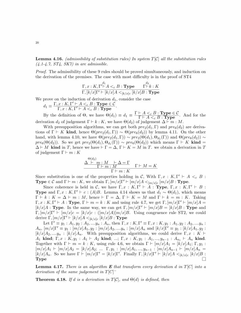
Lemma 4.16. (admissibility of substitution rules) In system T [C] all the substitution rules(4.1-4.7, ST4, SK7) in are admissible.
Proof. The admissibility of these 9 rules should be proved simultaneously, and induction onthe derivation of the premises. The case with most difficulty is in the proof of ST4
Γ, x : K,Γ′d1⊢A <c B : Type Γ
d2⊢k : K
Γ, [k/x]Γ′ ⊢ [k/x]A <[k/x]c [k/x]B : Type
We prove on the induction of derivation d1, consider the case
d1 ≡ Γ, x : K,Γ′ ⊢ A <c B : Type ∈ CΓ, x : K,Γ′ ⊢ A <c B : Type
.
By the definition of Θ, we have Θ(d1) ≡ d1 ≡ Γ ⊢ A <c B : Type ∈ CΓ ⊢ A <c B : Type
. And for the
derivation d2 of judgement Γ ⊢ k : K, we have Θ(d2) of judgement ∆ ⊢ m : M .With presupposition algorithms, we can get both pre2(d1,Γ) and pre6(d2) are deriva-
tions of Γ ⊢ K kind, hence Θ(pre2(d1,Γ)) ∼ Θ(pre6(d2)) by lemma 4.11. On the otherhand, with lemma 4.10, we have Θ(pre2(d1,Γ)) ∼ pre2(Θ(d1),Θd1(Γ)) and Θ(pre6(d2)) ∼pre6(Θ(d2)). So we get pre2(Θ(d1),Θd1(Γ)) ∼ pre6(Θ(d2)) which means Γ ⊢ K kind =∆ ⊢ M kind in T , hence we have ⊢ Γ = ∆, Γ ⊢ K = M in T . we obtain a derivation in Tof judgement Γ ⊢ m : K
∆Θ(d2)
⊢ m : M ⊢ ∆ = ΓΓ ⊢ m : M Γ ⊢ M = K
Γ ⊢ m : K
Since substitution is one of the properties holding in C, With Γ, x : K,Γ′ ⊢ A <c B :Type ∈ C and Γ ⊢ m : K, we obtain Γ, [m/x]Γ′ ⊢ [m/x]A <[m/x]c [m/x]B : Type.
Since coherence is held in C, we have Γ, x : K,Γ′ ⊢ A : Type, Γ, x : K,Γ′ ⊢ B :Type and Γ, x : K,Γ′ ⊢ c : (A)B. Lemma 4.14 shows us that d1 ∼ Θ(d1), which meansΓ ⊢ k : K = ∆ ⊢ m : M , hence ⊢ Γ = ∆, Γ ⊢ K = M and Γ ⊢ k = m : K. TakingΓ, x : K,Γ′ ⊢ A : Type, Γ ⊢ m = k : K and using rule 4.7, we get Γ, [m/x]Γ′ ⊢ [m/x]A =[k/x]A : Type. In the same way, we can get Γ, [m/x]Γ′ ⊢ [m/x]B = [k/x]B : Type andΓ, [m/x]Γ′ ⊢ [m/x]c = [k/x]c : ([m/x]A)[m/x]B. Using congruence rule ST2, we couldderive Γ, [m/x]Γ′ ⊢ [k/x]A <[k/x]c [k/x]B : Type
Let Γ′ ≡ y1 : A1, y2 : A2, ....yn : An, then Γ, x : K,Γ′ ≡ Γ, x : K, y1 : A1, y2 : A2, ....yn :An, [m/x]Γ′ ≡ y1 : [m/x]A1, y2 : [m/x]A2, ....yn : [m/x]An and [k/x]Γ′ ≡ y1 : [k/x]A1, y2 :[k/x]A2, ....yn : [k/x]An. With presupposition algorithms, we could derive Γ, x : K ⊢A1 kind; Γ, x : K, y1 : A1 ⊢ A2 kind; ...; Γ, x : K, y1 : A1, ..., yn−1 : An1 ⊢ An kind.Together with Γ ⊢ m = k : K, using rule 4.6, we obtain Γ ⊢ [m/x]A1 = [k/x]A1; Γ, y1 :[m/x]A1 ⊢ [m/x]A2 = [k/x]A2; ... Γ, y1 : [m/x]A1, ..., yn−1 : [m/x]An−1 ⊢ [m/x]An =[k/x]An. So we have Γ ⊢ [m/x]Γ′ = [k/x]Γ′. Finally Γ, [k/x]Γ′ ⊢ [k/x]A <[k/x]c [k/x]B :Type
Lemma 4.17. There is an algorithm E that transform every derivation d in T [C] into aderivation of the same judgement in T [C]−
Theorem 4.18. If d is a derivation in T [C], and Θ(d) is defined, then
21
4.4. About the prove.
We follow the prove of Sergei’s in [SL02], but there are some differences. There are someproblems which bring the prove in [SL02] into trouble. One is that in the defintion of Θ,and the induction proof of the lemmas and theorems, it didn’t check the cases of rules inR (where R is a set of rules with coercive judgements as conclusion). Another is that inthe proof of weakening and admissiblity of subsitution in T [R], the basis were not right.The inductive hypothsis in T could not be applied directly on the case that derivation is inT [R], since the premises are derivations in T [R] not in T .
In our prove, C is a set of coercion judgements, so we don’t need to worry about thecases in the inductions. When inductive hypothsis is in T , we
5. Conclusion and Future Work
In this paper, we have given a counter example to show that T [R], which is generated byextending type system T with a set of coercion rules R, is not a proper way to generatea type system with coercive subtyping. The extension system may not conservative overthe original one. And prove that T [C], which is generated by extending type system Twith a well-defined set of judgements for coercions C, is a conservative extension over T .We think the system T [C] is a more general formulation of extending type systems withcoercive subtype.
The original type system T we consider in this paper is a concrete type system UTTspecified in LF. We wish T could be an arbitrary consistent type system, but unluckily,this doesn’t hold. Very like the counter example for T [R] in section ??, we could thinka type system T with an unused rule with contains non-well typed premises, and with aconclusion which may cause inconsistent. Since this rule will not be used in T , T is stillconsistent. But once we extend T with coercive subtyping, the premise may be well typedvia coercions and the rule may be used, and inconsistency may be caused. What kind oftype system we shall consider of or what restrictions we shall make on the type system, isstill an interesting question.
References
[BF99] G.Barthe, M.J.Frade. Constructor subtyping. in :Proceedings of ESOP’99 LNCS1576, 1999.[BR00] G.Barthe, F.V.Raamsdonk. Constructor subtypinigin the Calculus of Inductive Constructions Pro-
ceedings of FOSSACS 00, LNCS 1794, 17-34, 2000.[CL01] P. Callahan, Z. Luo. An implementation of LF with coercive subtyping and universes. Journal of
Automated Reasoning, 27(1), 3-27, 2001.[Car88] L. Cardelli. Typechecking dependent types and subtypes Lecture Notes in Computer Science,
vol(306), 45 - 57, 1988.[CW85] L. Cardelli, P. Wegner. On Understanding Types, Data Abstraction, and Polymorphism. Computing
Surveys, 17(4), 471-522, 1985.[JLS98] A. Jones, Zhaohui Luo, Sergei Soloviev Some proof-thertic and algotrithmic aspects of coercive
subtyping Types for proofs and programs(eds, E.Gimenez and C. Paulin-Mohring), Proc of the Inter.Conf. TYPES’96, LNCS 1512, 1998.
[LL05] Y. Luo, Z. Luo. Transitivity in coercive subtyping. Information and Computation, 197:122-144,2005.
[Luo94] Z. Luo. Computation and Reasoning: A Type Theory for Computer Science. Oxford UniversityPress, 1994.
22
[Luo97] Z. Luo Coercive subtyping in type theory. Proc. of CSL’96, the 1996 Annual Conference of theEuropean Association for Computer Science Logic, Utrecht. LNCS 1258, 1997.
[Luo99] Z. Luo. Coercive subtyping. Journal of Logic and Computation., 9(1):105–130, 1999.[Luo05] Y. Luo. Cohernce and transitivity in coercive subtyping. PhD thesis, University of Durham, 2004.[Luo10] Z. Luo. Type-Theoretical Semantics with Coercive Subtyping. Semantics and Linguistic Theory,
Vol. 20 (SALT20), Vancouver. 2010.[LS99] Z. Luo, S. Soloviev. Dependent coercions. in: The 8th International Conference on Category Theory
and Computater Science(CTCS’99), Edinburg, Scortland. Electronic Notes in Theoretical ComputerScience, 29, 1999.
[Mar84] P. Martin-Lof. Intuitionistic type theory. Napoli, Bibliopolis, 1984.[Mar75] P. Martin-Lof. An Intuitionistic Theory of Types: Predicative Part. In: H.Rose and
J.C.Shepherdson editors, Logic Colloquium’73, North-Holland, 1975.[Mil78] R. Milner. A Theory of Type Polymorphism in Programming. Journal of Computer and System
Sciences, 17, 348-375, 1978.[Mit91] J.C Mitchell. Type inference with simple subtypes. Journal of Functional Programming, 1(2), 245-
286, 1991.[NPS90] B. Nordstrom, K. Petersson, and J. Smith. Programming in Martin-Lof ’s Type Theory: An Intro-
duction. Oxford University Press, 1990.[Sai97] A. Saibi Typing algorithm in type theory with inheritance Procedings of POPL97, 1997[SL02] S. Soloviev, Z. Luo. Coercion completion and conservativity in coercive subtyping. Annals of Pure
and Applied Logic(2002)

23
Appendix A. Rules of LF
The following give the rule of logical framework LF.
24
Appendix B. Presupposition algorithms
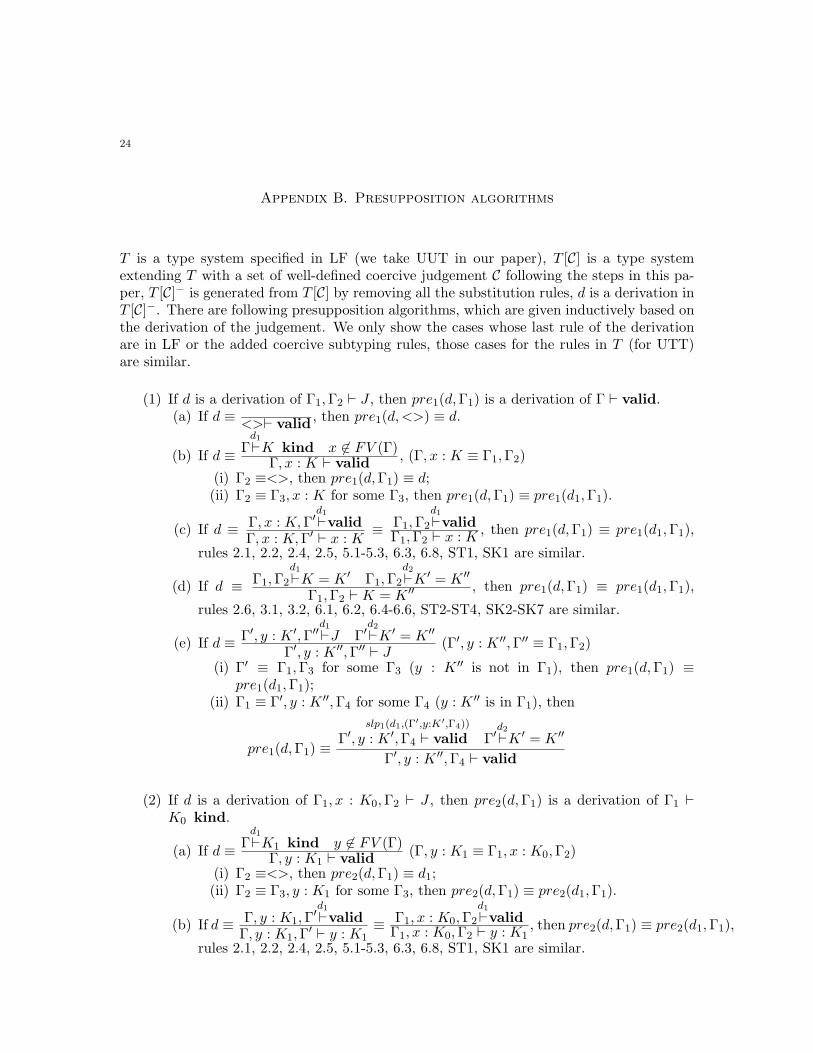
T is a type system specified in LF (we take UUT in our paper), T [C] is a type systemextending T with a set of well-defined coercive judgement C following the steps in this pa-per, T [C]− is generated from T [C] by removing all the substitution rules, d is a derivation inT [C]−. There are following presupposition algorithms, which are given inductively based onthe derivation of the judgement. We only show the cases whose last rule of the derivationare in LF or the added coercive subtyping rules, those cases for the rules in T (for UTT)are similar.
(1) If d is a derivation of Γ1,Γ2 ⊢ J , then pre1(d,Γ1) is a derivation of Γ ⊢ valid.(a) If d ≡
<>⊢ valid, then pre1(d,<>) ≡ d.
(b) If d ≡ Γd1⊢K kind x ∈ FV (Γ)
Γ, x : K ⊢ valid, (Γ, x : K ≡ Γ1,Γ2)
(i) Γ2 ≡<>, then pre1(d,Γ1) ≡ d;(ii) Γ2 ≡ Γ3, x : K for some Γ3, then pre1(d,Γ1) ≡ pre1(d1,Γ1).
(c) If d ≡ Γ, x : K,Γ′d1⊢validΓ, x : K,Γ′ ⊢ x : K
≡ Γ1,Γ2
d1⊢valid
Γ1,Γ2 ⊢ x : K, then pre1(d,Γ1) ≡ pre1(d1,Γ1),
rules 2.1, 2.2, 2.4, 2.5, 5.1-5.3, 6.3, 6.8, ST1, SK1 are similar.
(d) If d ≡ Γ1,Γ2
d1⊢K = K ′ Γ1,Γ2
d2⊢K ′ = K ′′
Γ1,Γ2 ⊢ K = K ′′ , then pre1(d,Γ1) ≡ pre1(d1,Γ1),
rules 2.6, 3.1, 3.2, 6.1, 6.2, 6.4-6.6, ST2-ST4, SK2-SK7 are similar.
(e) If d ≡ Γ′, y : K ′,Γ′′d1⊢J Γ′d2⊢K ′ = K ′′
Γ′, y : K ′′,Γ′′ ⊢ J(Γ′, y : K ′′,Γ′′ ≡ Γ1,Γ2)
(i) Γ′ ≡ Γ1,Γ3 for some Γ3 (y : K ′′ is not in Γ1), then pre1(d,Γ1) ≡pre1(d1,Γ1);
(ii) Γ1 ≡ Γ′, y : K ′′,Γ4 for some Γ4 (y : K ′′ is in Γ1), then
pre1(d,Γ1) ≡
slp1(d1,(Γ′,y:K′,Γ4))
Γ′, y : K ′,Γ4 ⊢ valid Γ′d2⊢K ′ = K ′′
Γ′, y : K ′′,Γ4 ⊢ valid
(2) If d is a derivation of Γ1, x : K0,Γ2 ⊢ J , then pre2(d,Γ1) is a derivation of Γ1 ⊢K0 kind.
(a) If d ≡ Γd1⊢K1 kind y ∈ FV (Γ)
Γ, y : K1 ⊢ valid(Γ, y : K1 ≡ Γ1, x : K0,Γ2)
(i) Γ2 ≡<>, then pre2(d,Γ1) ≡ d1;(ii) Γ2 ≡ Γ3, y : K1 for some Γ3, then pre2(d,Γ1) ≡ pre2(d1,Γ1).
(b) If d ≡ Γ, y : K1,Γ′d1⊢valid
Γ, y : K1,Γ′ ⊢ y : K1
≡ Γ1, x : K0,Γ2
d1⊢valid
Γ1, x : K0,Γ2 ⊢ y : K1, then pre2(d,Γ1) ≡ pre2(d1,Γ1),
rules 2.1, 2.2, 2.4, 2.5, 5.1-5.3, 6.3, 6.8, ST1, SK1 are similar.
25
(c) If d ≡ Γ1, x : K0,Γ2
d1⊢K = K ′ Γ1, x : K0,Γ2
d2⊢K ′ = K ′′
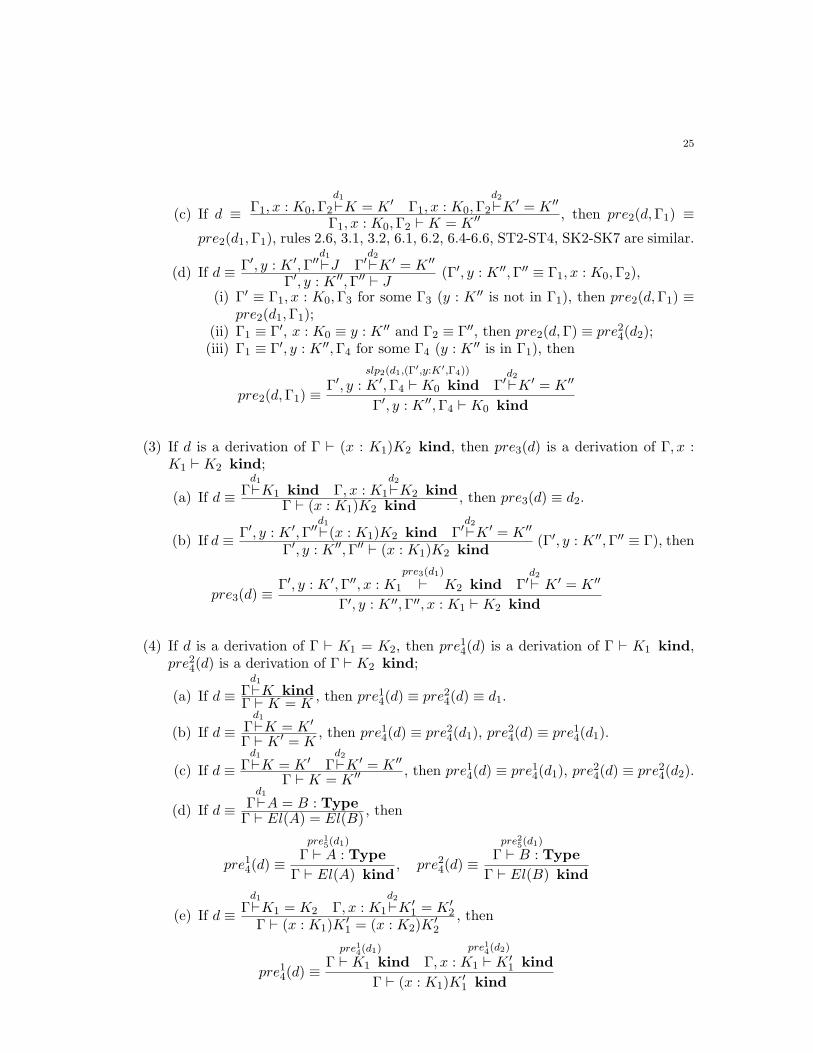
Γ1, x : K0,Γ2 ⊢ K = K ′′ , then pre2(d,Γ1) ≡pre2(d1,Γ1), rules 2.6, 3.1, 3.2, 6.1, 6.2, 6.4-6.6, ST2-ST4, SK2-SK7 are similar.
(d) If d ≡ Γ′, y : K ′,Γ′′d1⊢J Γ′d2⊢K ′ = K ′′
Γ′, y : K ′′,Γ′′ ⊢ J(Γ′, y : K ′′,Γ′′ ≡ Γ1, x : K0,Γ2),
(i) Γ′ ≡ Γ1, x : K0,Γ3 for some Γ3 (y : K ′′ is not in Γ1), then pre2(d,Γ1) ≡pre2(d1,Γ1);
(ii) Γ1 ≡ Γ′, x : K0 ≡ y : K ′′ and Γ2 ≡ Γ′′, then pre2(d,Γ) ≡ pre24(d2);(iii) Γ1 ≡ Γ′, y : K ′′,Γ4 for some Γ4 (y : K ′′ is in Γ1), then
pre2(d,Γ1) ≡
slp2(d1,(Γ′,y:K′,Γ4))
Γ′, y : K ′,Γ4 ⊢ K0 kind Γ′d2⊢K ′ = K ′′
Γ′, y : K ′′,Γ4 ⊢ K0 kind
(3) If d is a derivation of Γ ⊢ (x : K1)K2 kind, then pre3(d) is a derivation of Γ, x :K1 ⊢ K2 kind;
(a) If d ≡ Γd1⊢K1 kind Γ, x : K1
d2⊢K2 kind
Γ ⊢ (x : K1)K2 kind, then pre3(d) ≡ d2.
(b) If d ≡ Γ′, y : K ′,Γ′′d1⊢(x : K1)K2 kind Γ′d2⊢K ′ = K ′′
Γ′, y : K ′′,Γ′′ ⊢ (x : K1)K2 kind(Γ′, y : K ′′,Γ′′ ≡ Γ), then
pre3(d) ≡Γ′, y : K ′,Γ′′, x : K1
pre3(d1)
⊢ K2 kind Γ′d2⊢ K ′ = K ′′
Γ′, y : K ′′,Γ′′, x : K1 ⊢ K2 kind
(4) If d is a derivation of Γ ⊢ K1 = K2, then pre14(d) is a derivation of Γ ⊢ K1 kind,pre24(d) is a derivation of Γ ⊢ K2 kind;
(a) If d ≡ Γd1⊢K kind
Γ ⊢ K = K, then pre14(d) ≡ pre24(d) ≡ d1.
(b) If d ≡ Γd1⊢K = K ′
Γ ⊢ K ′ = K, then pre14(d) ≡ pre24(d1), pre
24(d) ≡ pre14(d1).
(c) If d ≡ Γd1⊢K = K ′ Γ
d2⊢K ′ = K ′′
Γ ⊢ K = K ′′ , then pre14(d) ≡ pre14(d1), pre24(d) ≡ pre24(d2).
(d) If d ≡ Γd1⊢A = B : Type
Γ ⊢ El(A) = El(B), then
pre14(d) ≡
pre15(d1)
Γ ⊢ A : Type
Γ ⊢ El(A) kind, pre24(d) ≡
pre25(d1)
Γ ⊢ B : Type
Γ ⊢ El(B) kind
(e) If d ≡ Γd1⊢K1 = K2 Γ, x : K1
d2⊢K ′
1 = K ′2
Γ ⊢ (x : K1)K′1 = (x : K2)K
′2
, then
pre14(d) ≡
pre14(d1)
Γ ⊢ K1 kindpre14(d2)
Γ, x : K1 ⊢ K ′1 kind
Γ ⊢ (x : K1)K′1 kind
26
pre24(d) ≡pre24(d1)
Γ ⊢ K2 kind
pre24(d2)
Γ, x : K1 ⊢ K2′ kind Γd1⊢K1 = K2
Γ, x : K2 ⊢ K ′2 kind
Γ ⊢ (x : K2)K′2 kind
(f) If d ≡ Γ′, y : K ′,Γ′′d1⊢K1 = K2 Γ′d2⊢K ′ = K ′′
Γ′, y : K ′′,Γ′′ ⊢ K1 = K2(Γ′, y : K ′′,Γ′′ ≡ Γ), then
pre14(d) ≡
pre14(d1)
Γ′, y : K ′,Γ′′ ⊢ K1 kind Γ′d2⊢K ′ = K ′′
Γ′, y : K ′′,Γ′′ ⊢ K1 kind
pre24(d) ≡
pre24(d1)
Γ′, y : K ′,Γ′′ ⊢ K2 kind Γ′d2⊢K ′ = K ′′
Γ′, y : K ′′,Γ′′ ⊢ K2 kind
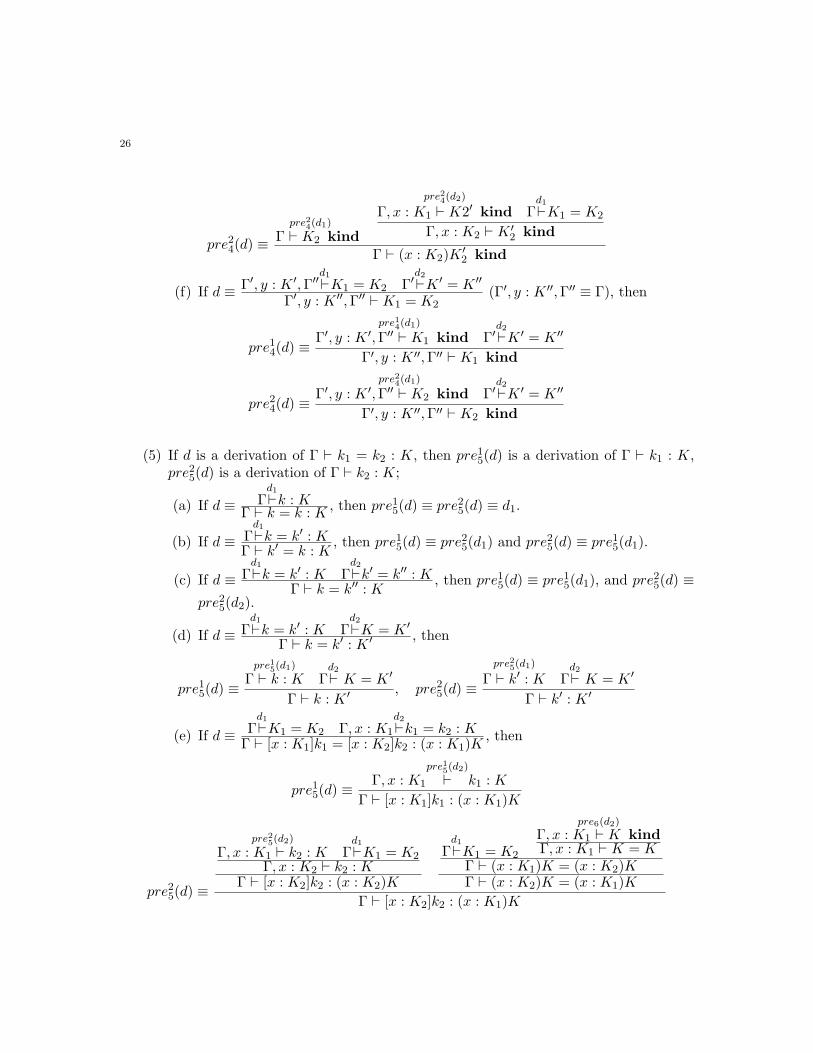
(5) If d is a derivation of Γ ⊢ k1 = k2 : K, then pre15(d) is a derivation of Γ ⊢ k1 : K,pre25(d) is a derivation of Γ ⊢ k2 : K;
(a) If d ≡ Γd1⊢k : K
Γ ⊢ k = k : K, then pre15(d) ≡ pre25(d) ≡ d1.
(b) If d ≡ Γd1⊢k = k′ : K
Γ ⊢ k′ = k : K, then pre15(d) ≡ pre25(d1) and pre25(d) ≡ pre15(d1).
(c) If d ≡ Γd1⊢k = k′ : K Γ
d2⊢k′ = k′′ : K
Γ ⊢ k = k′′ : K, then pre15(d) ≡ pre15(d1), and pre25(d) ≡
pre25(d2).
(d) If d ≡ Γd1⊢k = k′ : K Γ
d2⊢K = K ′
Γ ⊢ k = k′ : K ′ , then
pre15(d) ≡
pre15(d1)
Γ ⊢ k : K Γd2⊢ K = K ′
Γ ⊢ k : K ′ , pre25(d) ≡
pre25(d1)
Γ ⊢ k′ : K Γd2⊢ K = K ′
Γ ⊢ k′ : K ′
(e) If d ≡ Γd1⊢K1 = K2 Γ, x : K1
d2⊢k1 = k2 : K
Γ ⊢ [x : K1]k1 = [x : K2]k2 : (x : K1)K, then
pre15(d) ≡Γ, x : K1
pre15(d2)
⊢ k1 : K
Γ ⊢ [x : K1]k1 : (x : K1)K
pre25(d) ≡
pre25(d2)
Γ, x : K1 ⊢ k2 : K Γd1⊢K1 = K2
Γ, x : K2 ⊢ k2 : KΓ ⊢ [x : K2]k2 : (x : K2)K
Γd1⊢K1 = K2
pre6(d2)
Γ, x : K1 ⊢ K kindΓ, x : K1 ⊢ K = K
Γ ⊢ (x : K1)K = (x : K2)KΓ ⊢ (x : K2)K = (x : K1)K
Γ ⊢ [x : K2]k2 : (x : K1)K
27
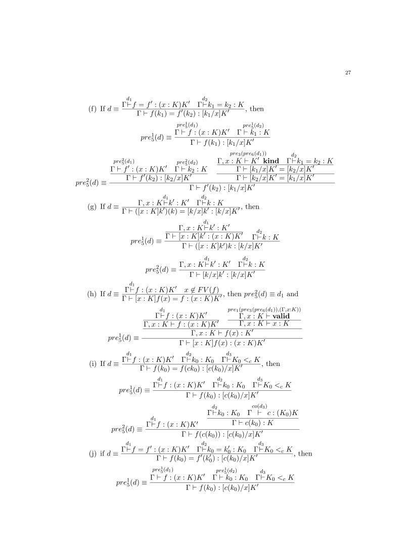
(f) If d ≡ Γd1⊢f = f ′ : (x : K)K ′ Γ
d2⊢k1 = k2 : K
Γ ⊢ f(k1) = f ′(k2) : [k1/x]K′ , then
pre15(d) ≡
pre15(d1)
Γ ⊢ f : (x : K)K ′pre15(d2)
Γ ⊢ k1 : K
Γ ⊢ f(k1) : [k1/x]K′
pre25(d) ≡
pre25(d1)
Γ ⊢ f ′ : (x : K)K ′pre25(d2)
Γ ⊢ k2 : KΓ ⊢ f ′(k2) : [k2/x]K
′
pre3(pre6(d1))
Γ, x : K ⊢ K ′ kind Γd2⊢k1 = k2 : K
Γ ⊢ [k1/x]K′ = [k2/x]K
′
Γ ⊢ [k2/x]K′ = [k1/x]K
′
Γ ⊢ f ′(k2) : [k1/x]K′
(g) If d ≡ Γ, x : Kd1⊢k′ : K ′ Γ
d2⊢k : K
Γ ⊢ ([x : K]k′)(k) = [k/x]k′ : [k/x]K ′ , then
pre15(d) ≡
Γ, x : Kd1⊢k′ : K ′
Γ ⊢ [x : K]k′ : (x : K)K ′Γd2⊢k : K
Γ ⊢ ([x : K]k′)k : [k/x]K ′
pre25(d) ≡Γ, x : K
d1⊢k′ : K ′ Γ
d2⊢k : K
Γ ⊢ [k/x]k′ : [k/x]K ′
(h) If d ≡ Γd1⊢f : (x : K)K ′ x ∈ FV (f)
Γ ⊢ [x : K]f(x) = f : (x : K)K ′ , then pre25(d) ≡ d1 and
pre15(d) ≡
Γd1⊢f : (x : K)K ′
Γ, x : K ⊢ f : (x : K)K ′
pre1(pre3(pre6(d1)),(Γ,x:K))
Γ, x : K ⊢ validΓ, x : K ⊢ x : K
Γ, x : K ⊢ f(x) : K ′
Γ ⊢ [x : K]f(x) : (x : K)K ′
(i) If d ≡ Γd1⊢f : (x : K)K ′ Γ
d2⊢k0 : K0 Γ
d3⊢K0 <c K
Γ ⊢ f(k0) = f(ck0) : [c(k0)/x]K′ , then
pre15(d) ≡Γd1⊢f : (x : K)K ′ Γ
d2⊢k0 : K0 Γ
d3⊢K0 <c K
Γ ⊢ f(k0) : [c(k0)/x]K′
pre25(d) ≡Γd1⊢f : (x : K)K ′
Γd2⊢k0 : K0 Γ
co(d3)
⊢ c : (K0)K
Γ ⊢ c(k0) : K
Γ ⊢ f(c(k0)) : [c(k0)/x]K′
(j) if d ≡ Γd1⊢f = f ′ : (x : K)K ′ Γ
d2⊢k0 = k′0 : K0 Γ
d3⊢K0 <c K
Γ ⊢ f(k0) = f ′(k′0) : [c(k0)/x]K′ , then
pre15(d) ≡
pre15(d1)
Γ ⊢ f : (x : K)K ′pre15(d2)
Γ ⊢ k0 : K0 Γd3⊢K0 <c K
Γ ⊢ f(k0) : [c(k0)/x]K′
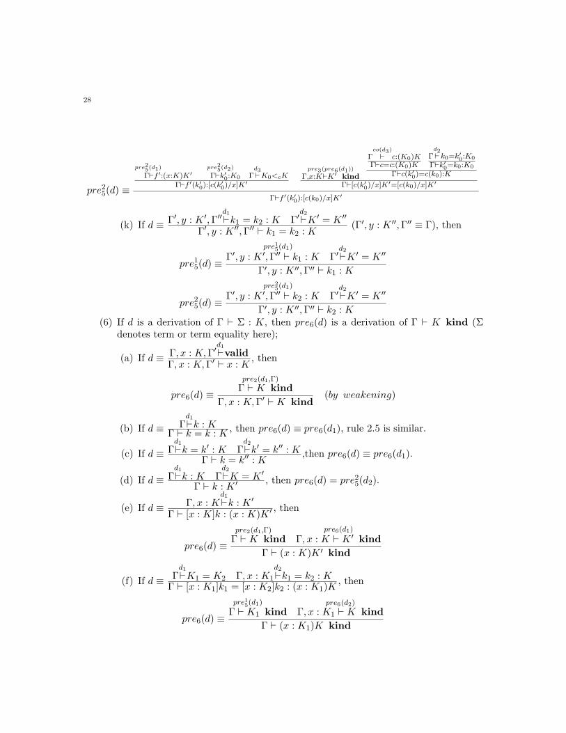
28
pre25(d) ≡
pre25(d1)
Γ⊢f ′:(x:K)K′pre25(d2)
Γ⊢k′0:K0 Γd3⊢K0<cK
Γ⊢f ′(k′0):[c(k′0)/x]K
′
pre3(pre6(d1))
Γ,x:K⊢K′ kind
Γco(d3)
⊢ c:(K0)KΓ⊢c=c:(K0)K
Γd2⊢ k0=k′0:K0
Γ⊢k′0=k0:K0
Γ⊢c(k′0)=c(k0):K
Γ⊢[c(k′0)/x]K′=[c(k0)/x]K′
Γ⊢f ′(k′0):[c(k0)/x]K′
(k) If d ≡ Γ′, y : K ′,Γ′′d1⊢k1 = k2 : K Γ′d2⊢K ′ = K ′′
Γ′, y : K ′′,Γ′′ ⊢ k1 = k2 : K(Γ′, y : K ′′,Γ′′ ≡ Γ), then
pre15(d) ≡
pre15(d1)
Γ′, y : K ′,Γ′′ ⊢ k1 : K Γ′d2⊢K ′ = K ′′
Γ′, y : K ′′,Γ′′ ⊢ k1 : K
pre25(d) ≡
pre25(d1)
Γ′, y : K ′,Γ′′ ⊢ k2 : K Γ′d2⊢K ′ = K ′′
Γ′, y : K ′′,Γ′′ ⊢ k2 : K(6) If d is a derivation of Γ ⊢ Σ : K, then pre6(d) is a derivation of Γ ⊢ K kind (Σ
denotes term or term equality here);
(a) If d ≡ Γ, x : K,Γ′d1⊢validΓ, x : K,Γ′ ⊢ x : K
, then
pre6(d) ≡pre2(d1,Γ)
Γ ⊢ K kind
Γ, x : K,Γ′ ⊢ K kind(by weakening)
(b) If d ≡ Γd1⊢k : K
Γ ⊢ k = k : K, then pre6(d) ≡ pre6(d1), rule 2.5 is similar.
(c) If d ≡ Γd1⊢k = k′ : K Γ
d2⊢k′ = k′′ : K
Γ ⊢ k = k′′ : K,then pre6(d) ≡ pre6(d1).
(d) If d ≡ Γd1⊢k : K Γ
d2⊢K = K ′
Γ ⊢ k : K ′ , then pre6(d) = pre25(d2).
(e) If d ≡ Γ, x : Kd1⊢k : K ′
Γ ⊢ [x : K]k : (x : K)K ′ , then
pre6(d) ≡pre2(d1,Γ)
Γ ⊢ K kindpre6(d1)
Γ, x : K ⊢ K ′ kind
Γ ⊢ (x : K)K ′ kind
(f) If d ≡ Γd1⊢K1 = K2 Γ, x : K1
d2⊢k1 = k2 : K
Γ ⊢ [x : K1]k1 = [x : K2]k2 : (x : K1)K, then
pre6(d) ≡
pre15(d1)
Γ ⊢ K1 kindpre6(d2)
Γ, x : K1 ⊢ K kind
Γ ⊢ (x : K1)K kind
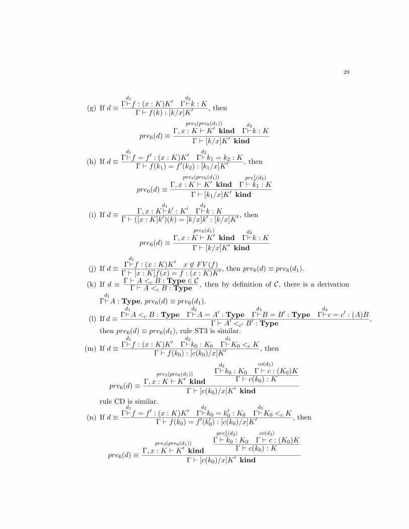
29
(g) If d ≡ Γd1⊢f : (x : K)K ′ Γ
d2⊢k : K
Γ ⊢ f(k) : [k/x]K ′ , then
pre6(d) ≡
pre3(pre6(d1))
Γ, x : K ⊢ K ′ kind Γd2⊢k : K
Γ ⊢ [k/x]K ′ kind
(h) If d ≡ Γd1⊢f = f ′ : (x : K)K ′ Γ
d2⊢k1 = k2 : K
Γ ⊢ f(k1) = f ′(k2) : [k1/x]K′ , then
pre6(d) ≡
pre3(pre6(d1))
Γ, x : K ⊢ K ′ kindpre14(d2)
Γ ⊢ k1 : K
Γ ⊢ [k1/x]K′ kind
(i) If d ≡ Γ, x : Kd1⊢k′ : K ′ Γ
d2⊢k : K
Γ ⊢ ([x : K]k′)(k) = [k/x]k′ : [k/x]K ′ , then
pre6(d) ≡
pre6(d1)
Γ, x : K ⊢ K ′ kind Γd2⊢k : K
Γ ⊢ [k/x]K ′ kind
(j) If d ≡ Γd1⊢f : (x : K)K ′ x ∈ FV (f)
Γ ⊢ [x : K]f(x) = f : (x : K)K ′ , then pre6(d) ≡ pre6(d1).
(k) If d ≡ Γ ⊢ A <c B : Type ∈ CΓ ⊢ A <c B : Type
, then by definition of C, there is a derivation
Γd1⊢A : Type, pre6(d) ≡ pre6(d1).
(l) If d ≡ Γd1⊢A <c B : Type Γ
d2⊢A = A′ : Type Γ
d3⊢B = B′ : Type Γ
d4⊢c = c′ : (A)B
Γ ⊢ A′ <c′ B′ : Type
,
then pre6(d) ≡ pre6(d1), rule ST3 is similar.
(m) If d ≡ Γd1⊢f : (x : K)K ′ Γ
d2⊢k0 : K0 Γ
d3⊢K0 <c K
Γ ⊢ f(k0) : [c(k0)/x]K′ , then
pre6(d) ≡pre3(pre6(d1))
Γ, x : K ⊢ K ′ kind
Γd2⊢k0 : K0
co(d3)
Γ ⊢ c : (K0)KΓ ⊢ c(k0) : K
Γ ⊢ [c(k0)/x]K′ kind
rule CD is similar.
(n) If d ≡ Γd1⊢f = f ′ : (x : K)K ′ Γ
d2⊢k0 = k′0 : K0 Γ
d3⊢K0 <c K
Γ ⊢ f(k0) = f ′(k′0) : [c(k0)/x]K′ , then
pre6(d) ≡pre3(pre6(d1))
Γ, x : K ⊢ K ′ kind
pre15(d2)
Γ ⊢ k0 : K0
co(d3)
Γ ⊢ c : (K0)KΓ ⊢ c(k0) : K
Γ ⊢ [c(k0)/x]K′ kind
30
(o) If d ≡ Γ′, y : K ′,Γ′′d1⊢Σ : K Γ′d2⊢K ′ = K ′′
Γ′, y : K ′′,Γ′′ ⊢ Σ : K(Γ′, y : K ′′,Γ′′ ≡ Γ), then
pre6(d) ≡
pre6(d1)
Γ′, y : K ′,Γ′′ ⊢ K kind Γ′d2⊢K ′ = K ′′
Γ′, y : K ′′,Γ′′ ⊢ K kind.
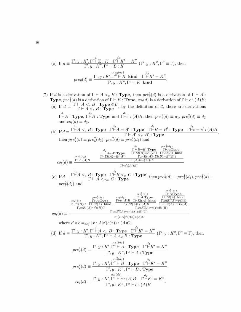
(7) If d is a derivation of Γ ⊢ A <c B : Type, then pre17(d) is a derivation of Γ ⊢ A :Type, pre27(d) is a derivation of Γ ⊢ B : Type, cot(d) is a derivation of Γ ⊢ c : (A)B;
(a) If d ≡ Γ ⊢ A <c B : Type ∈ CΓ ⊢ A <c B : Type
, by the definition of C, there are derivations
Γd1⊢A : Type, Γ
d2⊢B : Type and Γ
d3⊢c : (A)B, then pre17(d) ≡ d1, pre
27(d) ≡ d2
and cot(d) ≡ d3.
(b) If d ≡ Γd1⊢A <c B : Type Γ
d2⊢A = A′ : Type Γ
d3⊢B = B′ : Type Γ
d4⊢c = c′ : (A)B
Γ ⊢ A′ <c′ B′ : Type
,
then pre17(d) ≡ pre25(d2), pre27(d) ≡ pre25(d3) and
cot(d) ≡pre25(d4)
Γ⊢c′:(A)B
Γd2⊢A=A′:Type
Γ⊢El(A)=El(A′)
Γd3⊢B=B′:Type
Γ⊢El(B)=El(B′)
pre17(d1)
Γ⊢A:TypeΓ⊢El(A) kind
Γ,x:El(A)⊢El(B)=El(B′)Γ⊢(A)B=(A′)B′
Γ⊢c′:(A′)B′
(c) If d ≡ Γd1⊢A <c B : Type Γ
d2⊢B <c′ C : Type
Γ ⊢ A <c′◦c C : Type, then pre17(d) ≡ pre17(d1), pre
27(d) ≡
pre27(d2) and
cot(d) ≡
cot(d2)
Γ⊢c′:(B)C
pre17(d1)
Γ⊢A:TypeΓ⊢El(A) kind
Γ,x:El(A)⊢c′:(B)C
cot(d1)
Γ⊢c:(A)B
pre17(d1)
Γ⊢A:TypeΓ⊢El(A) kind
Γ,x:El(A)⊢c:(A)B
pre17(d1)
Γ⊢A:TypeΓ⊢El(A) kindΓ,x:El(A)⊢valid
Γ,x:El(A)⊢x:El(A)Γ,x:El(A)⊢c(x):El(B)
Γ,x:El(A)⊢c′(c(x)):El(C)
Γ⊢[x:A]c′(c(x)):(A)C
where c′ ◦ c =def [x : A]c′(c(x)) : (A)C;
(d) If d ≡ Γ′, y : K ′,Γ′′d1⊢A <c B : Type Γ′d2⊢K ′ = K ′′
Γ′, y : K ′′,Γ′′ ⊢ A <c B : Type(Γ′, y : K ′′,Γ′′ ≡ Γ), then
pre17(d) ≡
pre17(d1)
Γ′, y : K ′,Γ′′ ⊢ A : Type Γ′d2⊢K ′ = K ′′
Γ′, y : K ′′,Γ′′ ⊢ A : Type.
pre27(d) ≡
pre27(d1)
Γ′, y : K ′,Γ′′ ⊢ B : Type Γ′d2⊢K ′ = K ′′
Γ′, y : K ′′,Γ′′ ⊢ B : Type.
cot(d) ≡
cot(d1)
Γ′, y : K ′,Γ′′ ⊢ c : (A)B Γ′d2⊢K ′ = K ′′
Γ′, y : K ′′,Γ′′ ⊢ c : (A)B.
31
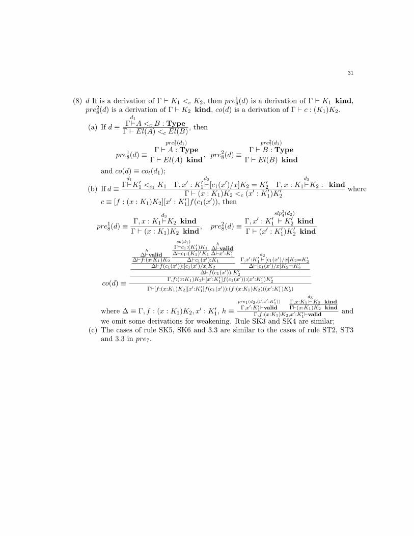
(8) d If is a derivation of Γ ⊢ K1 <c K2, then pre18(d) is a derivation of Γ ⊢ K1 kind,pre28(d) is a derivation of Γ ⊢ K2 kind, co(d) is a derivation of Γ ⊢ c : (K1)K2.
(a) If d ≡ Γd1⊢A <c B : Type
Γ ⊢ El(A) <c El(B), then
pre18(d) ≡
pre17(d1)
Γ ⊢ A : Type
Γ ⊢ El(A) kind, pre28(d) ≡
pre27(d1)
Γ ⊢ B : Type
Γ ⊢ El(B) kind
and co(d) ≡ cot(d1);
(b) If d ≡ Γd1⊢K ′
1 <c1 K1 Γ, x′ : K ′1
d2⊢ [c1(x′)/x]K2 = K ′
2 Γ, x : K1
d3⊢K2 : kind
Γ ⊢ (x : K1)K2 <c (x′ : K ′
1)K′2
where
c ≡ [f : (x : K1)K2][x′ : K ′
1]f(c1(x′)), then
pre18(d) ≡Γ, x : K1
d3⊢K2 kind
Γ ⊢ (x : K1)K2 kind, pre28(d) ≡
Γ, x′ : K ′1
slp24(d2)
⊢ K ′2 kind
Γ ⊢ (x′ : K ′1)K
′2 kind
co(d) ≡
∆h⊢valid
∆⊢f :(x:K1)K2
co(d1)
Γ⊢c1:(K′1)K1
∆⊢c1:(K1)′K1
∆h⊢valid
∆⊢x′:K′1
∆⊢c1(x′):K1
∆⊢f(c1(x′)):[c1(x′)/x]K2
Γ,x′:K′1
d2⊢ [c1(x′)/x]K2=K′
2∆⊢[c1(x′)/x]K2=K′
2∆⊢f(c1(x′)):K′
2Γ,f :(x:K1)K2⊢[x′:K′
1]f(c1(x′)):(x′:K′
1)K′2
Γ⊢[f :(x:K1)K2][x′:K′1]f(c1(x
′)):(f :(x:K1)K2)((x′:K′1)K
′2)
where ∆ ≡ Γ, f : (x : K1)K2, x′ : K ′
1, h ≡pre1(d2,(Γ,x′:K′
1))
Γ,x′:K′1⊢valid
Γ,x:K1
d3⊢K2 kind
Γ⊢(x:K1)K2 kind
Γ,f :(x:K1)K2,x′:K′1⊢valid
and
we omit some derivations for weakening. Rule SK3 and SK4 are similar;(c) The cases of rule SK5, SK6 and 3.3 are similar to the cases of rule ST2, ST3
and 3.3 in pre7.
32
Contexts and assumptions
(1.1)<>⊢ valid
(1.2)Γ ⊢ K kind x ∈ FV (Γ)
Γ, x : K ⊢ valid(1.3)
Γ, x : K,Γ′ ⊢ valid
Γ, x : K,Γ′ ⊢ x : K
(weakening)Γ,Γ′ ⊢ J, Γ ⊢ K kind x ∈ FV (Γ)
Γ, x : K,Γ′ ⊢ JGeneral equality rules
(2.1)Γ ⊢ K kind
Γ ⊢ K = K(2.2)
Γ ⊢ K = K ′
Γ ⊢ K ′ = K(2.3)
Γ ⊢ K = K ′ Γ ⊢ K ′ = K ′′
Γ ⊢ K = K ′′
(2.4)Γ ⊢ k : K
Γ ⊢ k = k : K(2.5)
Γ ⊢ k = k′ : K
Γ ⊢ k′ = k : K(2.6)
Γ ⊢ k = k′ : K Γ ⊢ k′ = k′′ : K
Γ ⊢ k = k′′ : KEquality typing rules
(3.1)Γ ⊢ k : K Γ ⊢ K = K ′
Γ ⊢ k : K ′ (3.2)Γ ⊢ k = k′ : K Γ ⊢ K = K ′
Γ ⊢ k = k′ : K ′
(3.3)Γ, x : K,Γ′ ⊢ J Γ ⊢ K = K ′
Γ, x : K ′,Γ′ ⊢ JSubstitution rules
(4.1)Γ, x : K,Γ′ ⊢ valid Γ ⊢ k : K
Γ, [k/x]Γ′ ⊢ valid
(4.2)Γ, x : K,Γ′ ⊢ K ′ kind Γ ⊢ k : K
Γ, [k/x]Γ′ ⊢ [k/x]K ′ kind(4.3)
Γ, x : K,Γ′ ⊢ k′ : K ′ Γ ⊢ k : K
Γ, [k/x]Γ′ ⊢ [k/x]k′ : [k/x]K ′
(4.4)Γ, x : K,Γ′ ⊢ K ′ = K ′′ Γ ⊢ k : K
Γ, [k/x]Γ′ ⊢ [k/x]K ′ = [k/x]K ′′ (4.5)Γ, x : K,Γ′ ⊢ k′ = k′′ : K ′ Γ ⊢ k : K
Γ, [k/x]Γ′ ⊢ [k/x]k′ = [k/x]k′′ : [k/x]K ′
(4.6)Γ, x : K,Γ′ ⊢ K ′ kind Γ ⊢ k = k′ : K
Γ, [k/x]Γ′ ⊢ [k/x]K ′ = [k′/x]K ′ (4.7)Γ, x : K,Γ′ ⊢ k′ : K ′ Γ ⊢ k1 = k2 : K
Γ, [k1/x]Γ′ ⊢ [k1/x]k′ = [k2/x]k′ : [k1/x]K ′
The kind Type
(5.1)Γ ⊢ valid
Γ ⊢ Type kind(5.2)
Γ ⊢ A : Type
Γ ⊢ El(A) kind(5.3)
A = B : Type
Γ ⊢ El(A) = El(B)
Dependent product kinds
(6.1)Γ ⊢ K kind Γ, x : K ⊢ K ′ kind
Γ ⊢ (x : K)K ′ kind(6.2)
Γ ⊢ K1 = K2 Γ, x : K1 ⊢ K ′1 = K ′
2
Γ ⊢ (x : K1)K ′1 = (x : K2)K ′
2
(6.3)Γ, x : K ⊢ k : K ′
Γ ⊢ [x : K]k : (x : K)K ′ (6.4)(ξ)Γ ⊢ K1 = K2 Γ, x : K1 ⊢ k1 = k2 : K
Γ ⊢ [x : K1]k1 = [x : K2]k2 : (x : K1)K
(6.5)Γ ⊢ f : (x : K)K ′ Γ ⊢ k : K
Γ ⊢ f(k) : [k/x]K ′ (6.6)Γ ⊢ f = f ′ : (x : K)K ′ Γ ⊢ k1 = k2 : K
Γ ⊢ f(k1) = f ′(k2) : [k1/x]K ′
(6.7)(β)Γ, x : K ⊢ k′ : K ′ Γ ⊢ k : K
Γ ⊢ ([x : K]k′)(k) = [k/x]k′ : [k/x]K ′ (6.8)(η)Γ ⊢ f : (x : K)K ′ x ∈ FV (f)
Γ ⊢ [x : K]f(x) = f : (x : K)K ′
Figure 1: The inference rules of LF