# 1003

Conspicuous Consumption and Race: Evidence from South Africa

by

Wolfhard Kaus

Max Planck Institute of Economics Evolutionary Economics Group Kahlaische Str. 10 07745 Jena, Germany Fax: ++49-3641-686868

The Papers on Economics and Evolution are edited by the Evolutionary Economics Group, MPI Jena. For editorial correspondence,

please contact: evopapers@econ.mpg.de

ISSN 1430-4716

© by the author

#1003

Conspicuous Consumption and Race:

Evidence from South Africa∗

Wolfhard Kaus†

Abstract

A century ago, Thorstein Veblen introduced socially contingent con-sumption into the economic literature. This paper complements the scarceempirical literature by testing his conjecture on South African householddata and finds that Black and Coloured households spend relatively moreon visible consumption than comparable White households. In an emerg-ing economy context, this is especially important as it carries implicationsfor spending on future assets. This paper explores whether the differencesin visible expenditures can be explained with a signaling model of statusseeking. Among Black households, spending on visible consumption isfound to change predictably with different reference group incomes.

Keywords: Conspicuous consumption, Signaling, Status, South Africa

JEL classification: D12, D83, J15, O12

∗This paper would not have been possible without the support by Servaas van der Bergwho kindly provided access to the data used. For helpful discussions and valuable commentsI would like to thank Tommaso Ciarli, Alessio Moneta, Dieter von Fintel, Benjamin Volland,Simon Wiederhold, Ulrich Witt, and Derek Yu. The usual disclaimer applies.†Max Planck Institute of Economics, Evolutionary Economics Group, Kahlaische Straße

10, 07745 Jena, Germany, kaus@econ.mpg.de.

1

#1003

1 Introduction

It is usually observed that expenditure patterns differ across as well as withincountries. A large body of theoretical and empirical contributions to demandtheory explains these differences in terms of variation in relative prices and in-come (see, e.g., Blundell (1988) for a survey and Selvanathan and Selvanathan(1993, 2004) for more empirical applications). An important assumption of thisapproach holds that the utility functions, and thus the underlying preferences,are similar. Nevertheless, anecdotal evidence shows that even at a given point intime and within the same country, some groups seem to spend more on certaintypes of goods. In a recent study Charles, Hurst, and Roussanov (2009) ex-plore such a particularity as they empirically access the differences in spendingon conspicuous consumption across races. They study U.S. household spend-ing on “visible consumption” using the Consumer Expenditure Survey (CES)database, an ongoing rotating panel data set, for the period 1986 to 2002. Vis-ible consumption is defined in terms of consumption items “that are readilyobservable in anonymous social interactions, and that are portable across thoseinteractions” (ibid p. 426). Moreover, consuming more of these goods shouldsignal “better economic circumstances” (ibid p. 431). In line with anecdotalevidence, Charles, Hurst, and Roussanov (2009) find a significant difference inspending patterns across races. After controlling for differences in permanentincome and demographics, Blacks and Hispanics spend about 30 percent moreon visible consumption than Whites.1 As visible consumption belongs to therealm of conspicuous consumption, it is straightforward to assume that the dif-ference in spending is (at least to some extent) explained by social interactionswith one’s reference group. Accordingly, Charles, Hurst, and Roussanov (2009)use a signaling model of status seeking to explain the observed phenomenon.Using this approach, the authors show that the statistically significant differ-ence in visible consumption vanishes after they control for mean reference groupincome. The results suggest that the initially found differences can be explainedby differences in the social environment. To be consistent with the assumptionof similar utility functions, these findings should hold not only across but alsowithin social groups. Even for each race separately, the two hypotheses can beconfirmed for the case of the U.S.

In light of the above, it would be especially useful to extend the analysisby Charles, Hurst, and Roussanov (2009) to less affluent countries for at leasttwo reasons. First, if individuals spend relatively more on visible consumption,(sooner or later) they will have to spend relatively less on other consumptioncategories. This will be particularly relevant if individuals among comparablyless affluent groups spend more on visible consumption, because it might bearimplications for their capacity to catch up to higher income levels. Charles,Hurst, and Roussanov (2009) show that on average Black and Hispanic house-holds seem to spend less on education, health, and food. Accordingly, if spendingon visible consumption crowds out spending on future assets among householdswith less affluent reference groups in a high income country like the U.S., asimilar finding in a less affluent country might carry implications for our under-standing of poverty. Second, testing the predictions of the signaling model ofstatus seeking in a less affluent and economically more unequal country offers

1The households are referred to as Black, Hispanic, Coloured, or White if the head of thehousehold has reported one of these categories as her social affiliation.

2

#1003

a more challenging environment for the underlying assumption of similar util-ity functions across different social groups. As South Africa consists of socialgroups with different cultural backgrounds, showing different income distribu-tions across groups and high inequality within groups, this country appears tobe exceptionally suited as a field of study.

This paper first assesses differences in spending on visible consumption acrosssocial groups in South Africa. Indeed, Coloured and Black households, whosemean income is much less than that of White households, are found to spend onaverage about 35 to 50 percent more on visible consumption than comparableWhite households. It is furthermore tested whether the differences in spendingon visible consumption can be explained by a model that incorporates sociallycontingent concerns for status. In line with the predictions of the signalingmodel of status seeking, the reference group’s mean income (as a proxy for so-cial environment) is found to account for the difference in visible expenditures.However, it is concluded that socially contingent differential spending on visi-ble consumption cannot be confirmed for each group separately. The differentresults for the South African subpopulations point to the fact that differentgroups may develop different ways to express their relative position within a so-ciety. Second, the paper assesses whether the importance of positional concernschanges with income. With rising income, a higher share of visible consumptionexpenditures is found to be socially contingent among the Black population.Overall, the paper contributes additional evidence for the existence of sociallycontingent consumption behavior as described by Veblen (1899). To the au-thor’s knowledge, this is the first paper that shows the validity of this behaviorand assesses the extent of social contingency using consumer expenditure datain a less affluent country context.2

The remainder of the paper is organized as follows. The next section reviewsthe related literature on conspicuous consumption and outlines the signalingmodel of status seeking as well as its predictions. Section 2 introduces thedata set and definitions used in the paper. In section 3, the between groupdifferences in visible expenditures are assessed and the suitability of the signalingstatus model in explaining the between group differences as a socially contingentphenomenon is tested. The fourth and last section summarizes the results andconcludes.

2 Related Literature and Model Predictions

Veblen (1899) was one of the first economists to systematically introduce statusconsiderations into economic theory. Fundamental to his “Theory of the leisureclass” is the assumption that individuals compare each other on the basis of theireconomic achievements. Moreover, he emphasized that these interpersonal com-parisons are important for human behavior as they constitute the individual’srecognition by others. As, according to Veblen (1899, p. 24f.), esteem by fellowhuman beings is the basis for self-respect, missing recognition by them wouldlower the individual’s self-assessment. To satisfy the need for self-respect, indi-viduals aim to have at least as much as their own reference group. To be noticed

2This is not to disregard earlier works on certain facets of conspicuous consumption. See,e.g., Bloch, Rao, and Desai (2004) regarding spending on wedding celebrations as a means tosignal status in rural India.

3

#1003

by others and to satisfy the desire for social recognition, individuals show theirwealth to others. As wealth is usually unobserved, Veblen (1899) identifies twodifferent ways to demonstrate one’s position in society. One variant is conspicu-ous leisure such as demonstratively engaging in everything but productive work.The second variant investigated here is conspicuous consumption, where visi-ble consumption of certain goods, signaling a higher position in interpersonalexchanges, is used to demonstrate one’s status.

The type of behavior sketched so far may give rise to certain dynamics withina society. If individuals from lower income groups aspire to the living standardof higher income groups, the demand for the relevant goods increases. Higherincome groups, however, have an incentive to distinguish themselves from lowerincome groups and thus direct their expenditures to more visible goods. Fur-thermore, Veblen (1899) infers that conspicuous consumption is even more im-portant as social cohesion decreases and mobility rises. The more anonymousand the more frequent individuals interactions with others are, the more conspic-uous consumption matters as a means to signal one’s relative position. In morenarrow economic terms, conspicuous consumption can be framed as an economicexternality. A broad range of economic works have focused on economic impli-cations and possible policy recommendations with regard to such an externality(see, e.g., Duesenberry 1949, Frank 1985, Bagwell and Bernheim 1996, Glazerand Konrad 1996, Cowan, Cowan, and Swann 1997).3

While Veblens work was rich in illustrating manifold facets of status-seekingbehavior, the present paper takes a more narrow approach to positional concernsby investigating spending on highly visible goods suited to signal one’s usuallyunobserved wealth. The basic idea has been elaborated in different signalingstatus models (Ireland 1994, Cole, Mailath, and Postlewaite 1995, Glazer andKonrad 1996, Corneo and Jeanne 1998, to mention a few). In accordance withsuch models, Charles, Hurst, and Roussanov (2009) derive a simple signalingframework for empirically investigating visible consumption. In their model, in-dividuals belong to certain reference groups whose income distribution is known.Individually unobserved income is spent on an observable and an unobservablegood. Utility is derived from spending on both kinds of goods as well as status,which is society’s inference about an individual’s income. Status is defined asthe expected value of an individual’s income given her observable spending onconspicuous consumption and the group she belongs to. Under the assumptionthat individuals maximize utility with respect to their budget constraint andsociety’s beliefs about an individual’s income, Charles, Hurst, and Roussanov(2009) derive the following predictions:

• Spending on conspicuous consumption increases with own income.

• If average group income rises, spending on conspicuous consumption de-creases.

For the present analysis the second prediction is particularly relevant as it incor-porates the group’s income distribution as a socially contingent factor, explain-ing the level of visible consumption. The intuition behind the second predictioncan be formulated as follows. Among comparable households, those living in amore affluent environment have a relatively less favorable position within their

3The importance of relative status has also been demonstrated in the context of subjectivewell-being; see, e.g., Dynan and Ravina (2007).

4

#1003

reference group. They should therefore spend relatively less on visible consump-tion.

If this conjecture is correct, it should be possible to show that any particu-larities in visible consumption across social groups vanish, or at least diminish,when the reference group’s average income is controlled for. Moreover, as theunderlying signaling model of status seeking assumes the similarity of utilityfunctions across groups, differential spending patterns on visible consumptionshould be observed within and across social groups.

3 Data and Definitions

The data used in this paper have been collected by Statistics South Africa(StatsSA). In the years 1995, 2000, and 2005, an income and expenditure sur-vey (IES) was conducted. It contains information on sources of incomes as wellas on the purchase of a wide variety of goods and services (Orkin 1997). De-signed to cover a representative sample of South African households, the samplesize consists of 29,582 households in 1995, 26,263 in 2000, and 21,144 in 2005,respectively.

Working with the data raises two problems. First, the structure of the IES2005 series differs from preceding surveys (Yu 2008). Second, it has occasionallybeen questioned whether the IES of 2000 meets a fully representative standard(see, e.g., Burger, van der Berg, and Nieftagodien 2004, van der Berg, Louw,and Yu 2008). Regarding the first problem, the classification of expenditureitems was changed from the Standard Trade Classification to the UN Statis-tics Division’s Classification of Individual Consumption According to Purpose(COICOP) in 2005. Moreover, the data collection methodology changed fromrecall to diary method. Besides these differences, imputed rent has been in-troduced as a new item. To account for these changes, some adjustments arenecessary.4 The second problem concerns mainly procedural weaknesses of the2000 IES sample. Due to migration between the 1996 census and the collectionof IES data for 2000, the survey is known to overrepresent the Black populationwhile underrepresenting the White population (Ozler 2007).5

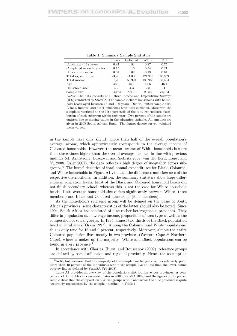
The summary statistics in Table 1 clearly show the huge differences in in-come and total expenditures across subgroups. On average, Black households

4The income and expenditure items compiled in 1995 and 2000 were recategorized accord-ing to the COICOP structure. Furthermore, the 2005 values of income, housing & utilitiesas well as total expenditures have to be corrected for the value of imputed rent to be com-parable to prior IES series. Although the change of methods from recall to diary methodmay also diminish comparability, von Fintel (2007) finds no systematic change in estimatingincome elasticities of aggregated product categories that can be attributed to the change inmethodology.

5Additionally, a higher share of zero values in food expenditures as well as greater differ-ences between total income and total expenditures have been found. In accordance with asuggestion by Ozler (2007), the 2000 sample was reweighted to match up with the populationshares in the 2001 census. Burger, van der Berg, and Nieftagodien (2004) use different meth-ods to correct for the observed IES 2000 deficiencies. Their results show surprising robustnessin parameter estimates, especially for more aggregated and less frequently purchased productcategories. The adjustments made and the results by Burger, van der Berg, and Nieftago-dien (2004) have encouraged the author to cautiously analyze the pooled data. To check therobustness of the results, all regressions in the paper were rerun without the IES 2000 data.Although the magnitude of some coefficients changed slightly, none of the results rely on theinclusion of the IES 2000 data.

5

#1003

Table 1: Summary Sample StatisticsBlack Coloured White Full

Education < 12 years 0.84 0.82 0.27 0.75Completed secondary school 0.15 0.16 0.54 0.21Education: degree 0.01 0.02 0.19 0.04Total expenditures 23,951 41,005 121,913 40,369Total income 31,701 56,991 183,965 56,584Age 46.2 46.1 47.6 46.4Household size 4.2 4.3 2.8 4Sample size 54,164 8,916 9,083 72,163

Notes: The data consists of all three Income and Expenditure Surveys(IES) conducted by StatsSA. The sample includes households with house-hold heads aged between 18 and 100 years. Due to limited sample size,Asians, Indians, and other minorities have been excluded. Moreover, thesample is restricted to the 99th percentile of the total expenditure distri-bution of each subgroup within each year. Two percent of the sample areomitted due to missing values in the education variable. All amounts aregiven in 2005 South African Rand. The figures denote survey weightedmean values.

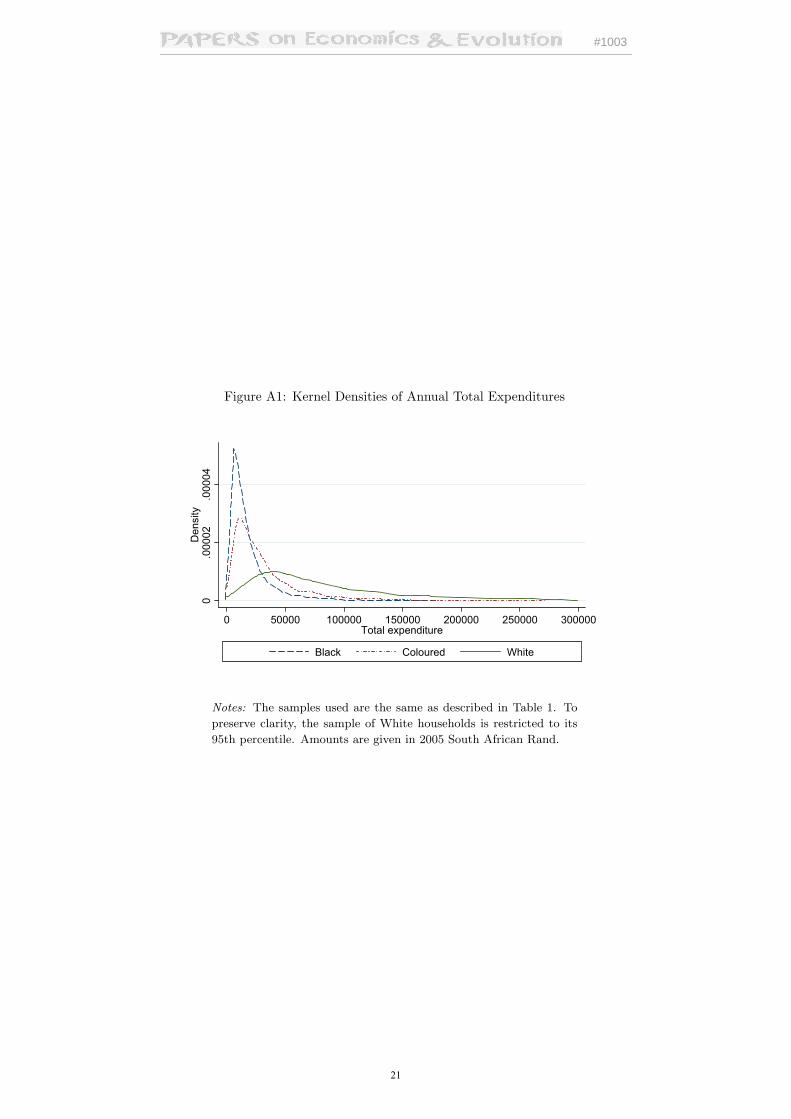
in the sample have only slightly more than half of the overall population’saverage income, which approximately corresponds to the average income ofColoured households. However, the mean income of White households is morethan three times higher than the overall average income. In line with previousfindings (cf. Armstrong, Lekezwa, and Siebrits 2008, van der Berg, Louw, andYu 2008, Ozler 2007), the data reflects a high degree of inequality across sub-groups.6 The kernel densities of total annual expenditures for Black, Coloured,and White households in Figure A1 visualize the differences and skewness of therespective distributions. In addition, the summary statistics show large differ-ences in education levels. Most of the Black and Coloured household heads didnot finish secondary school, whereas this is not the case for White householdheads. Last, average household size differs significantly between White (threemembers) and Black and Coloured households (four members).

As the household’s reference group will be defined on the basis of SouthAfrica’s provinces, some characteristics of the latter should also be noted. Since1994, South Africa has consisted of nine rather heterogeneous provinces. Theydiffer in population size, average income, proportions of area type as well as thecomposition of social groups. In 1995, almost two thirds of the Black populationlived in rural areas (Orkin 1997). Among the Coloured and White populations,this is only true for 16 and 9 percent, respectively. Moreover, almost the entireColoured population lives mostly in two provinces (Western Cape & NorthernCape), where it makes up the majority. White and Black populations can befound in every province.7

In accordance with Charles, Hurst, and Roussanov (2009), reference groupsare defined by social affiliation and regional proximity. Hence the assumption

6Note, furthermore, that the majority of the sample can be perceived as relatively poor.More than 40 percent of the individuals within the sample live on less than the lower-boundpoverty line as defined by StatsSA (Yu 2008).

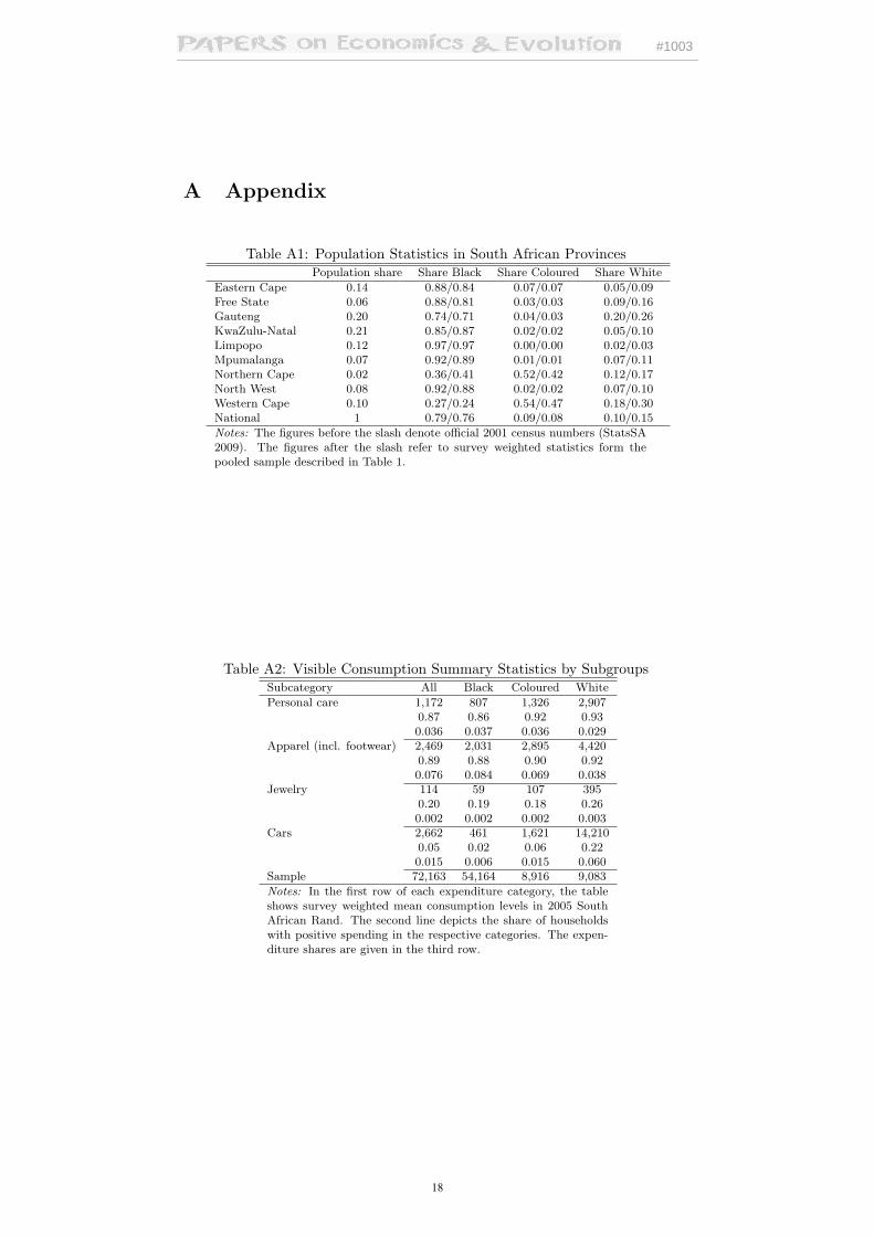
7Table A1 provides an overview of the populations distribution across provinces. A com-parison of South African census estimates in 2001 (StatsSA 2009) and the figures of the pooledsample show that the composition of social groups within and across the nine provinces is quiteaccurately represented by the sample described in Table 1.

6

#1003

is that Blacks (Coloureds, Whites) compare themselves only to other Blacks(Coloureds, Whites). It is further assumed that these reference groups can bedefined at a provincial level. For the inference of one’s income in anonymousinteractions, it is thus necessary to know one’s social affiliation and place ofresidence. Given the fact that most social interactions take place in the indi-viduals residential environment, it is straightforward to assume that this kindof knowledge is available to the observer. The arguably rough definition of ref-erence groups is claimed to be justified by two reasons. Even after apartheid,it has been recognized that race is still an important factor in social inter-actions in South Africa. This has been shown in several areas like the labormarket, the education system as well as residential environments (see, e.g.,Rospaba 2002, Moodley and Adam 2000). Further evidence is provided by arepresentative survey of the Institute for Justice and Reconciliation, which showsthat levels of interracial contact remain low (IJR 2010). About one quarter ofthe respondents report to have no verbal contacts with other groups in dailylife. Even more, about 50 percent, never socialize with individuals from differentgroups. The second reason, which may justify the broad definition of referencegroups, is related to the goods considered. In contrast to luxuries such as bigTV sets or costly tableware, which are visible only to a narrow peer group,this paper concentrates on conspicuous consumption goods that are portableand easily observable in anonymous interactions (as defined in the first sectionunder the term visible consumption). Therefore it is claimed that a more nar-rowly defined reference group would need much more specific assumptions and,accordingly, also a different model.

The classification of what is perceived to be visible consumption is an empir-ical task. For the U.S., Heffetz (2007) as well as Charles, Hurst, and Roussanov(2009) conducted a survey for this purpose. Whereas the telephone survey con-ducted by Heffetz (2007) was a random sample of the U.S. population over 18years, the survey by Charles, Hurst, and Roussanov (2009) was made amongbusiness students of the University of Chicago. According to the students’ opin-ions, spending on apparel, accessories, such as watches and jewelry, personalcare, and vehicles, are the most visible signs of better economic circumstancesin anonymous interactions. In Heffetz’s survey, among the readily observablegoods, cigarettes, cars, clothing, and jewelry are ranked highest in terms of vis-ibility. Thus, both surveys show quite similar results. For South Africa such asurvey is unfortunately not available. In this paper, a similar classification tothat for the U.S. is used. The visible consumption basket as defined by Charles,Hurst, and Roussanov (2009) is not explicitly restricted to particular products.Each item represents a category which may correspond to different products andservices in the U.S. and South Africa. However, spending on these categoriesmay still serve as a means to convey information about one’s status. Despiteother functional aspects served by these items, it would be hard to maintainthat goods which constitute outward appearance do not send any signals aboutthe economic status of a person in South Africa. It could, of course, be the casethat these signals are less important. If so, no systematic differences in spendingon the visible consumption basket should be found or explained by the signalingstatus model.

7

#1003

4 Empirical Investigation

This section starts out by assessing the differences in visible expenditures acrosssocial groups. The following subsection tests the predictions of the signalingmodel of status seeking outlined in section 2. Furthermore, the degrees of socialcontingency are estimated.

4.1 Assessing the differences

To begin with, spending on visible consumption is compared across social groups.Therefore log spending on the pooled basket of visible goods and services V isiis regressed on group dummies indicating a household as being Black Bli orColoured Coli, the log of a household’s permanent income pInci, a vector ofdemographic indicators Demi, i.e., area type, age, age squared, and family sizeas well as a vector of year dummies Yri. The corresponding regression can beformulated as follows:

ln(V isi) = β0 +β1 ∗Bli+β2 ∗Coli+γ ∗ ln(pInci)+δ ∗Demi + ε∗Yri +εi. (1)

Permanent income is usually measured by total expenditure. In like cir-cumstances, the measure is perceived as being more suitable than income as itallows to account for realized total expenditures that are larger or lower thanactual income, making total expenditures a smoother measure of income. Note,furthermore, that the log-log formulation of the regression equation allows to in-terpret its coefficient γ as (permanent) income elasticity of visible consumptionexpenditures. However, the permanent income measure does not come withoutflaws. Charles, Hurst, and Roussanov (2009) point to the fact that total expen-ditures are an endogenous variable to any components of total expenditures.Measurement errors in these components may, moreover, translate into mea-surement errors in the composite. Hence the log of total expenditures needs tobe instrumented. In a first approach, a set of instruments is applied, which is asclose as possible to the specification of Charles, Hurst, and Roussanov (2009),which, in turn, is a vector of current and permanent income controls. The setcontains a dummy for positive current income, log of current income, the levelof current income, a cubic in the level of current income as well as dummies forthree different levels of education (below secondary school, finished secondaryschool, degree).8 In a second approach, the education variables are excludedfrom the instruments. Since age and family size are assumed to directly in-fluence spending on visible consumption, it appears to be straightforward toassume that education might also directly influence the dependent variable.Accordingly, the set of education variables is used as predictor variables in thesecond approach. Tests of the statistical validity of different sets of instrumentssuggest a specification with log of current income as a single instrument.9

In Table 2, the differences between White, Black, and Coloured householdsare explored sequentially. Specification I estimates the unconditional differences

8To exactly match the authors specification, a series of one-digit industry and occupationcodes would also have to be included. This kind of data is unfortunately not available.

9Although F -stats and partial R2 on all instrument sets are sufficient, the large sampledemands cautiousness. In the second approach, the result of the weak identification testexceeds the Stock and Yogo (2005) critical values by far. This provides additional evidenceagainst weak-instrument concerns.

8

#1003

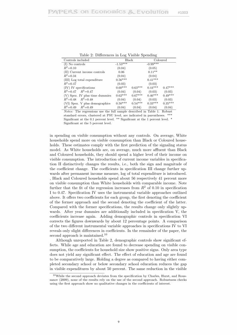
Table 2: Differences in Log Visible SpendingControls included Black Coloured

(I) No controls -1.53*** -0.99***R2=0.10 (0.04) (0.05)(II) Current income controls 0.06 0.11**R2=0.34 (0.04) (0.04)(III) Log total expenditure 0.56*** 0.41***R2=0.47 (0.03) (0.03)(IV) IV specifications 0.60*** 0.63*** 0.44*** 0.47***R2=0.47 R2=0.47 (0.04) (0.04) (0.03) (0.03)(V) Spez. IV plus time dummies 0.62*** 0.67*** 0.46*** 0.49***R2=0.48 R2=0.48 (0.04) (0.04) (0.03) (0.03)(VI) Spez. V plus demographics 0.50*** 0.54*** 0.33*** 0.35***R2=0.49 R2=0.49 (0.04) (0.04) (0.04) (0.04)

Notes: The regressions use the full sample described in Table 1. Robuststandard errors, clustered at PSU level, are indicated in parentheses. ***Significant at the 0.1 percent level. ** Significant at the 1 percent level. *Significant at the 5 percent level.

in spending on visible consumption without any controls. On average, Whitehouseholds spend more on visible consumption than Black or Coloured house-holds. These estimates comply with the first prediction of the signaling statusmodel. As White households are, on average, much more affluent than Blackand Coloured households, they should spend a higher level of their income onvisible consumption. The introduction of current income variables in specifica-tion II distinctively changes the results, i.e., both the sign and magnitude ofthe coefficient change. The coefficients in specification III change further up-wards after permanent income measure, log of total expenditure is introduced., Black and Coloured households spend about 56 respectively 41 percent moreon visible consumption than White households with comparable income. Notefurther that the fit of the regression increases from R2 of 0.10 in specificationI to 0.47. Specification IV uses the instrumental variable approaches outlinedabove. It offers two coefficients for each group, the first denoting the coefficientof the former approach and the second denoting the coefficient of the latter.Compared with the former specifications, the results change only slightly up-wards. After year dummies are additionally included in specification V, thecoefficients increase again. Adding demographic controls in specification VIcorrects the figures downwards by about 12 percentage points. A comparisonof the two different instrumental variable approaches in specifications IV to VIreveals only slight differences in coefficients. In the remainder of the paper, thesecond approach is maintained.10

Although unreported in Table 2, demographic controls show significant ef-fects. While age and education are found to decrease spending on visible con-sumption, the coefficients for household size show positive signs. Only area typedoes not yield any significant effect. The effect of education and age are foundto be comparatively large. Holding a degree as compared to having either com-pleted secondary school or below secondary school education reduces the gapin visible expenditures by about 50 percent. The same reduction in the visible

10While the second approach deviates from the specification by Charles, Hurst, and Rous-sanov (2009), none of the results rely on the use of the second approach. Robustness checksusing the first approach show no qualitative changes in the coefficients of interest.

9

#1003

spending gap can be found for households with heads older than 55 as comparedto younger than 35. Moreover, within the regression the coefficient for log totalexpenditures γ is larger than one (1.32). As γ represents the income elasticity,the visible consumption basket represents luxury goods and services.11 Theluxury property implies that with increasing income relatively more is spent onvisible consumption, which again confirms the first prediction of the signalingmodel.

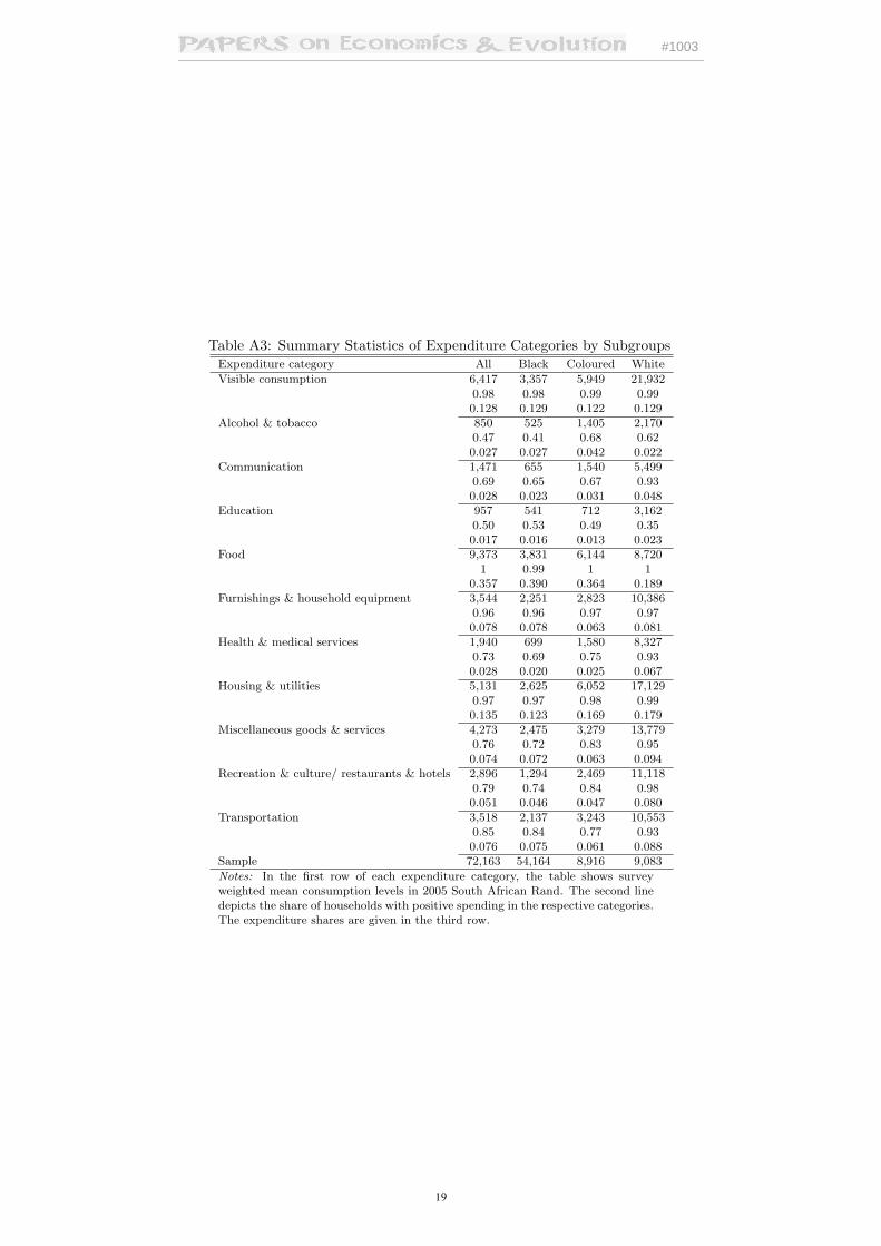
Overall, the first results in Table 2 indicate partial parallels to the findings inthe U.S., where the households of Black and Hispanic minorities spend 23 to 26percent more on visible consumption than White households with comparableincome and demographic backgrounds. Similarly, a gap in visible consumptionspending can be found in South Africa, where Black households, which consti-tute the majority of the overall population, spend about 50 percent more onvisible consumption than their White counterparts. These figures are substan-tial in absolute terms. Given that average spending of White households onvisible consumption is about 21,932 Rand a year (see Table A3), the above re-sult implies that comparable Black households, on average, spend 10,966 Randmore on visible consumption per year.

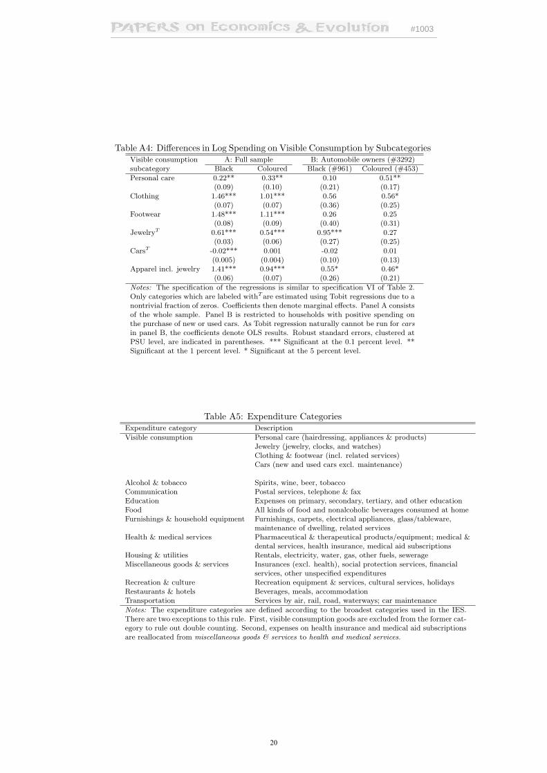
A closer examination of visible consumption components reveals a fairlyconsistent picture (see panel A in Table A4). Although the coefficients forparticular components differ in size, they uniformly show positive differences.A negative coefficient can only be found for cars.12 However, its magnitude isnegligible. The same pattern holds if only car owners are considered (panel Bof Table A4). Overall, the differences are most pronounced for clothing andfootwear , followed by jewelry and personal care.

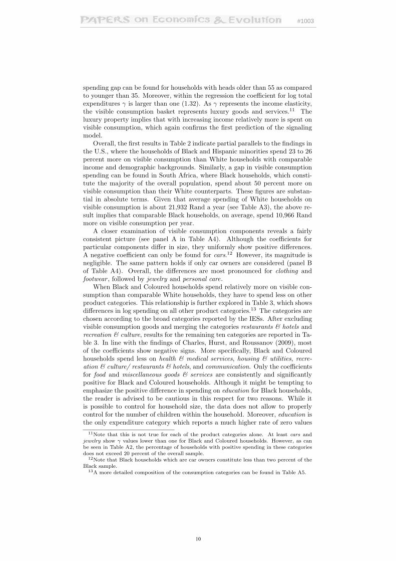
When Black and Coloured households spend relatively more on visible con-sumption than comparable White households, they have to spend less on otherproduct categories. This relationship is further explored in Table 3, which showsdifferences in log spending on all other product categories.13 The categories arechosen according to the broad categories reported by the IESs. After excludingvisible consumption goods and merging the categories restaurants & hotels andrecreation & culture, results for the remaining ten categories are reported in Ta-ble 3. In line with the findings of Charles, Hurst, and Roussanov (2009), mostof the coefficients show negative signs. More specifically, Black and Colouredhouseholds spend less on health & medical services, housing & utilities, recre-ation & culture/ restaurants & hotels, and communication. Only the coefficientsfor food and miscellaneous goods & services are consistently and significantlypositive for Black and Coloured households. Although it might be tempting toemphasize the positive difference in spending on education for Black households,the reader is advised to be cautious in this respect for two reasons. While itis possible to control for household size, the data does not allow to properlycontrol for the number of children within the household. Moreover, education isthe only expenditure category which reports a much higher rate of zero values

11Note that this is not true for each of the product categories alone. At least cars andjewelry show γ values lower than one for Black and Coloured households. However, as canbe seen in Table A2, the percentage of households with positive spending in these categoriesdoes not exceed 20 percent of the overall sample.

12Note that Black households which are car owners constitute less than two percent of theBlack sample.

13A more detailed composition of the consumption categories can be found in Table A5.

10

#1003

Table 3: Differences in Log Expenditure CategoriesExpenditure category Black Coloured

Alcohol & tobaccoT -1.44*** 0.39***(0.08) (0.08)

CommunicationT -0.84*** -1.17***(0.08) (0.07)

EducationT 0.60*** -0.13(0.06) (0.07)

Food 0.10*** 0.21***(0.03) (0.03)

Furnishings & household equipment 0.40*** 0.07(0.06) (0.06)

Health & medical servicesT -0.61*** -0.85***(0.07) (0.07)

Housing & utilities -0.73*** -0.24***(0.05) (0.05)

Miscellaneous goods & servicesT 0.94*** 0.90***(0.07) (0.08)

Recreation & culture/ restaurants & hotelsT -0.14* -0.12*(0.06) (0.06)

Transportation 0.75*** -0.35***(0.07) (0.08)

Notes: The specification of the regressions is similar to specification IVof Table 2. Only categories which are labeled withT are estimated usingTobit regressions due to a nontrivial fraction of zeros. Coefficients thendenote marginal effects. Robust standard errors, clustered at PSU level,are indicated in parentheses. *** Significant at the 0.1 percent level. **Significant at the 1 percent level. * Significant at the 5 percent level.

for White households as compared to remaining households in the sample (seeTable A3).

4.2 Explaining the differences

In this subsection, it is tested whether the differences in spending on visibleconsumption can be explained by the signaling model outlined in section 2.The second prediction, If average group income rises, spending on conspicuousconsumption decreases, is of special interest here because it incorporates thegroup’s income distribution as a socially contingent factor explaining the levelof visible consumption. Among comparable households, which differ only withrespect to their mean group income, those living in a more affluent environmenthave a relatively less favorable position within their reference group and shouldtherefore spend relatively less on visible consumption. To maintain the under-lying assumption of similar utility functions across groups, this should be truenot only across social groups but also within each group. Moreover, the resultsof the second prediction are explored in more detail to disentangle the sociallycontingent and the autonomous shares of visible consumption.

To test the second prediction, the following regression is estimated separately

11

#1003

Table 4: Within-Group Differences in Log Visible ExpendituresControls (I) (II)

Log mean group income (Black) -0.26***(0.06)

Log mean group income (White) 0.10(0.13)

Notes: The regressions use the full sample described in Ta-ble 1. Specifications I and II are similar to specification VIin Table 1 except for the omission of group dummies and theintroduction of log mean own group income. Specifications Iand II are estimated separately by subgroups. Robust stan-dard errors, clustered at PSU level, are indicated in paren-theses. *** Significant at the 0.1 percent level. ** Significantat the 1 percent level. * Significant at the 5 percent level.

for Black and White households:14

ln(V isi) = β0 + α ∗ ln(Incµk,t) + γ ∗ ln(pInci) + δ ∗Demi + ε ∗Yri + ζi, (2)

where k refers to one of 27 provinces/race units and Incµk,t denotes the averageincome of a certain group in one of the nine provinces in a certain year.

The results in Table 4 confirm the second prediction only partially. Thenegative coefficient in specification I of Table 4 complies with the prediction.Its value of -0.26 implies that if mean group income doubles, the expenditures onvisible consumption decrease by 26 percent. Thus, on average, about one quarterof the expenditures on the visible consumption basket turns out to be sociallycontingent. The same coefficient estimated for White households (specificationII) does not comply with the second prediction as it fails to show any significantnegative effect. Accordingly, the conjecture that, independent of social groupaffiliation, spending on visible consumption is a general means to signal statuscannot be confirmed. The results thus challenge the assumption of similar utilityfunctions. However, this is not to deny any social contingency among Whitehouseholds. Two explanations may apply here. Either for historical reasonsWhites do have no need to signal status at all, or they simply use different meansto signal their relative position within their reference group. Both explanationswould be in line with Mason (1998), who acknowledges different status-relatedbehavior between old-established wealthy individuals and those whose incomehas increased only recently.

Thus far, the results confirm the social contingency hypothesis at least forBlacks, who make up the largest share of the South African population. How-ever, although such an effect could be found on average, it is unclear whetherits magnitude is evenly distributed. In fact, one could argue that the magnitudemay be more pronounced among the poorest households. This would amount toclaiming that relatively poor households are more inclined to care about statuswhich would, in turn, translate into higher socially contingent shares of visi-ble consumption. It is thus explored whether the former effect systematicallychanges across the income distribution of the Black population. Using the par-titioning approach (see, e.g., Yip and Tsang 2007), regression (2) is rerun with

14A separate regression for Coloured households is omitted as the skewed distribution ofColoureds across provinces (see Table A1) does not allow to obtain reliable estimates of meangroup income for most provinces.

12

#1003

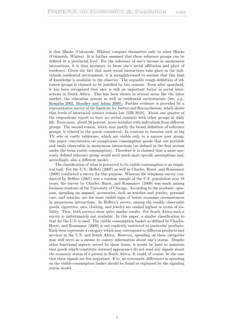
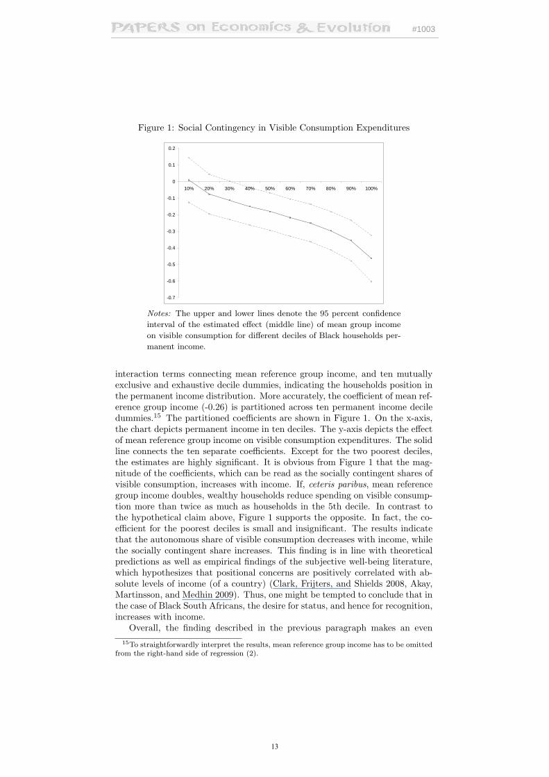
Figure 1: Social Contingency in Visible Consumption Expenditures

-0.7

-0.6

-0.5

-0.4

-0.3

-0.2

-0.1

0

0.1

0.2

10% 20% 30% 40% 50% 60% 70% 80% 90% 100%

Notes: The upper and lower lines denote the 95 percent confidence

interval of the estimated effect (middle line) of mean group income

on visible consumption for different deciles of Black households per-

manent income.

interaction terms connecting mean reference group income, and ten mutuallyexclusive and exhaustive decile dummies, indicating the households position inthe permanent income distribution. More accurately, the coefficient of mean ref-erence group income (-0.26) is partitioned across ten permanent income deciledummies.15 The partitioned coefficients are shown in Figure 1. On the x-axis,the chart depicts permanent income in ten deciles. The y-axis depicts the effectof mean reference group income on visible consumption expenditures. The solidline connects the ten separate coefficients. Except for the two poorest deciles,the estimates are highly significant. It is obvious from Figure 1 that the mag-nitude of the coefficients, which can be read as the socially contingent shares ofvisible consumption, increases with income. If, ceteris paribus, mean referencegroup income doubles, wealthy households reduce spending on visible consump-tion more than twice as much as households in the 5th decile. In contrast tothe hypothetical claim above, Figure 1 supports the opposite. In fact, the co-efficient for the poorest deciles is small and insignificant. The results indicatethat the autonomous share of visible consumption decreases with income, whilethe socially contingent share increases. This finding is in line with theoreticalpredictions as well as empirical findings of the subjective well-being literature,which hypothesizes that positional concerns are positively correlated with ab-solute levels of income (of a country) (Clark, Frijters, and Shields 2008, Akay,Martinsson, and Medhin 2009). Thus, one might be tempted to conclude that inthe case of Black South Africans, the desire for status, and hence for recognition,increases with income.

Overall, the finding described in the previous paragraph makes an even15To straightforwardly interpret the results, mean reference group income has to be omitted

from the right-hand side of regression (2).

13

#1003

Table 5: Differences in Log Visible ExpendituresControls (I) (II)

Black dummy 0.54*** 0.08(0.04) (0.09)

Coloured dummy 0.35*** 0.01(0.04) (0.06)

Log mean own group income -0.29***(0.05)

Notes: The regressions use the full sample described in Ta-ble 1. Specification I is similar to specification VI in Table 2.Specification II additionally includes the log of mean referencegroup income. Robust standard errors, clustered at PSU level,are indicated in parentheses. *** Significant at the 0.1 percentlevel. ** Significant at the 1 percent level. * Significant at the5 percent level.

stronger case for the suitability of the signaling status model in tracing so-cial contingencies in consumption expenditures. Although the socially contin-gent share in visible consumption increases with income, the different incen-tives to consume conspicuously seem to explain that, at every level of income,Black households spend relatively more on visible consumption than comparableWhite households.

To complete the analysis, one remaining implication of the signaling statusmodel is tested. If concerns for status determine spending on visible consump-tion, the differences in spending should vanish, or at least diminish, after thereference group’s average income is controlled for. Table 5 contrasts the resultsof specification VI in Table 2 with results of a similar regression that includesmean reference group income as an additional control variable. The group vari-ables in the second specifications show a striking difference. The coefficient forColoured as well as for Black households drops sharply and loses significance.Moreover, the coefficient of mean reference group income is clearly significantand negative.16 Concerns for status thus appear to be an important factor inexplaining differential spending on visible consumption across social groups.

5 Conclusion

South African society is characterized by huge differences within and betweensocial groups. This paper examines only a very small part of these differences,namely those in the spending on a particular consumption category by socialgroups. It is shown that Coloureds and Blacks spend between 30 to 50 percentmore on a basket of visible consumption goods and services than comparableWhites. This finding is especially enlightening because the partly socially con-tingent expenditures on visible consumption among Black and Coloured house-holds, which are on average much less affluent than White ones, imply lowerspending on other consumption categories. Regarding the data under consider-ation, lower expenditures on health & medical services are the most remarkable.

In the empirical analysis, it is tested whether the differences in spending on16Robustness checks reveal that no alternative measure of reference group income, such

as the overall province average or the provincial mean of a certain group alone, is able toinvalidate the group dummies.

14

#1003

visible consumption can be explained by a signaling model that incorporates so-cially contingent concerns for status. Under the assumption that status-relatedexpenditures depend on the relative position within the own reference group,the influence of mean reference group income on group differences in visiblespending is tested. In line with the predictions of the signaling model, the ref-erence group’s mean income is found to account for these differences. Havinga more favorable position within the own reference group, i.e., having a lessaffluent reference group than comparable households, may thus explain highervisible spending of Black and Coloured households.

Counter to the model’s assumptions, differential spending on visible con-sumption cannot be confirmed for each group separately. Although the expec-tations are confirmed for the largest share of the population, socially contingentspending on visible consumption is not observable within the White population.This indicates that among White South Africans, visible consumption appearsto be a less viable sign of their economic position. However, this finding doesnot deny any social contingency among White South Africans. Most probably itis only the signaling channels that differ from those of U.S. Americans or BlackSouth Africans. Nevertheless, the different results for South African subpop-ulations point to the fact that different groups may develop different ways toexpress their relative position within a society. Therefore it may not always bejustified to assume similar utility functions across different groups.

Moreover, the paper has assessed whether the importance of status consider-ations changes with income. As spending on visible consumption is found to bea rather poor proxy to capture status-related consumption among Whites, theanalysis is restricted to the Black subpopulation. With rising income, a highershare of visible consumption expenditures is found to be socially contingent.This finding indicates steady differences in the importance of status, and there-fore the desire for recognition with rising income. The overall results confirmthe importance of Veblen’s concept of socially contingent status considerationsin an economically emerging country.

References

Akay, A., P. Martinsson, and H. Medhin (2009): “Does Positional ConcernMatter in Poor Societies? Evidence from a Survey Experiment in RuralEthiopia,” IZA Discussion Papers 4354, Institute for the Study of Labor.

Armstrong, P., B. Lekezwa, and K. Siebrits (2008): “Poverty in SouthAfrica: A profile based on recent household surveys,” Stellenbosch EconomicWorking Papers 04/2008.

Bagwell, L. S., and B. D. Bernheim (1996): “Veblen Effects in a Theoryof Conspicuous Consumption,” American Economic Review, 86(3), 349–73.

Bloch, F., V. Rao, and S. Desai (2004): “Wedding Celebrations as Con-spicuous Consumption: Signaling Social Status in Rural India,” Journal ofHuman Resources, 39(3), 675–695.

Blundell, R. (1988): “Consumer Behaviour: Theory and Empirical Evidence–A Survey,” The Economic Journal, 98(389), 16–65.

15

#1003

Burger, R., S. van der Berg, and S. Nieftagodien (2004): “ConsumptionPatterns of South Africa’s Rising Middle-Class: Correcting for MeasurementErrors,” Paper presented at the conference of the Center for the Study ofAfrican Economies on Poverty Reduction, Growth and Human Developmentin Africa, Oxford.

Charles, K. K., E. Hurst, and N. Roussanov (2009): “Conspicuous Con-sumption and Race,” The Quarterly Journal of Economics, 124(2), 425–467.

Clark, A. E., P. Frijters, and M. A. Shields (2008): “Relative Income,Happiness, and Utility: An Explanation for the Easterlin Paradox and OtherPuzzles,” Journal of Economic Literature, 46(1), 95–144.

Cole, H. L., G. J. Mailath, and A. Postlewaite (1995): “Incorporatingconcern for relative wealth into economic models,” Federal Reserve Bank ofMinneapolis Quarterly Review, 13(9), 12–21.

Corneo, G., and O. Jeanne (1998): “Social organization, status, and savingsbehavior,” Journal of Public Economics, 70(1), 37–51.

Cowan, R., W. Cowan, and G. M. P. Swann (1997): “A model of demandwith interactions among consumers,” International Journal of Industrial Or-ganization, 15(6), 711–732.

Duesenberry, J. S. (1949): Income, Saving and the Theory of ConsumerBehavior. Harvard University Press, Cambridge.

Dynan, K. E., and E. Ravina (2007): “Increasing Income Inequality, ExternalHabits, and Self-Reported Happiness,” American Economic Review, 97(2),226–231.

Frank, R. H. (1985): “The Demand for Unobservable and Other NonpositionalGoods,” American Economic Review, 75(1), 101–16.

Glazer, A., and K. A. Konrad (1996): “A Signaling Explanation for Char-ity,” American Economic Review, 86(4), 1019–28.

Heffetz, O. (2007): “Conspicuous Consumption and Ex-penditure Visibility: Measurement and Application,”http://forum.johnson.cornell.edu/faculty/heffetz/papers/consp.pdf.

IJR (2010): “South African Reconciliation Barometer: Report 2009,”http://www.ijr.org.za/politicalanalysis/reconcbar/sa-barometer-research-reports/sarb-report-2009.pdf (05.01.2010).

Ireland, N. J. (1994): “On limiting the market for status signals,” Journal ofPublic Economics, 53(1), 91–110.

Mason, R. S. (1998): The Economics of Conspicuous Consumption: Theoryand Thought since 1700. Edward Elgar, Cheltenham.

Moodley, K., and H. Adam (2000): “Race and Nation in Post-ApartheidSouth Africa,” Current Sociology, 48(3), 51–69.

16

#1003

Orkin, M. (1997): “Earning and spending in South Africa. Selected findingsof the 1995 Income and Expenditure Survey,” Pretoria: Central StatisticalService.

Ozler, B. (2007): “Not Separate, Not Equal: Poverty and Inequality in Post-apartheid South Africa,” Economic Development and Cultural Change, 55,487–529.

Rospaba, S. (2002): “How Did Labour Market Racial Discrimination EvolveAfter The End Of Apartheid?,” South African Journal of Economics, 70(1),185–217.

Selvanathan, S., and E. A. Selvanathan (1993): “A Cross-Country Anal-ysis of Consumption Patterns,” Applied Economics, 25(9), 1245–59.

(2004): “Empirical regularities in South African consumption pat-terns,” Applied Economics, 36(20), 2327–2333.

StatsSA (2009): “Digital Census Atlas. Census 2001,”http://www.statssa.gov.za/census2001/digiAtlas/index.html (12.03.2009).

Stock, J. H., and M. Yogo (2005): “Testing for weak instruments in linear IVregression,” in Identification and Inference for Econometric Models: Essaysin Honor of Thomas Rothenberg, ed. by D. W. K. Andrews, and J. H. Stock,pp. 80–108. Cambridge University Press, Cambridge.

van der Berg, S., M. Louw, and D. Yu (2008): “Post-Transition PovertyTrends Based On An Alternative Data Source,” South African Journal ofEconomics, 76(1), 58–76.

Veblen, T. (1899): The Theory of the Leisure Class: Economic Study of In-stitutions. Random House, New York.

von Fintel, D. (2007): “An intertemporal comparison of expenditure elas-ticities in South Africa - what do estimates from Income and ExpenditureSurveys reveal about diary and recall enumeration?,” unpublished report forStatistics South Africa.

Yip, P. S. L., and E. W. K. Tsang (2007): “Interpreting dummy vari-ables and their interaction effects in strategy research,” Strategic Organiza-tion, 5(1), 13–30.

Yu, D. (2008): “The comparability of Income and Expenditure Surveys 1995,2000 and 2005/2006,” Stellenbosch Economic Working Papers 11/2008.

17

#1003

A Appendix

Table A1: Population Statistics in South African ProvincesPopulation share Share Black Share Coloured Share White

Eastern Cape 0.14 0.88/0.84 0.07/0.07 0.05/0.09Free State 0.06 0.88/0.81 0.03/0.03 0.09/0.16Gauteng 0.20 0.74/0.71 0.04/0.03 0.20/0.26KwaZulu-Natal 0.21 0.85/0.87 0.02/0.02 0.05/0.10Limpopo 0.12 0.97/0.97 0.00/0.00 0.02/0.03Mpumalanga 0.07 0.92/0.89 0.01/0.01 0.07/0.11Northern Cape 0.02 0.36/0.41 0.52/0.42 0.12/0.17North West 0.08 0.92/0.88 0.02/0.02 0.07/0.10Western Cape 0.10 0.27/0.24 0.54/0.47 0.18/0.30National 1 0.79/0.76 0.09/0.08 0.10/0.15

Notes: The figures before the slash denote official 2001 census numbers (StatsSA2009). The figures after the slash refer to survey weighted statistics form thepooled sample described in Table 1.

Table A2: Visible Consumption Summary Statistics by SubgroupsSubcategory All Black Coloured White

Personal care 1,172 807 1,326 2,9070.87 0.86 0.92 0.930.036 0.037 0.036 0.029

Apparel (incl. footwear) 2,469 2,031 2,895 4,4200.89 0.88 0.90 0.920.076 0.084 0.069 0.038

Jewelry 114 59 107 3950.20 0.19 0.18 0.260.002 0.002 0.002 0.003

Cars 2,662 461 1,621 14,2100.05 0.02 0.06 0.220.015 0.006 0.015 0.060

Sample 72,163 54,164 8,916 9,083

Notes: In the first row of each expenditure category, the tableshows survey weighted mean consumption levels in 2005 SouthAfrican Rand. The second line depicts the share of householdswith positive spending in the respective categories. The expen-diture shares are given in the third row.

18

#1003

Table A3: Summary Statistics of Expenditure Categories by SubgroupsExpenditure category All Black Coloured White

Visible consumption 6,417 3,357 5,949 21,9320.98 0.98 0.99 0.990.128 0.129 0.122 0.129

Alcohol & tobacco 850 525 1,405 2,1700.47 0.41 0.68 0.620.027 0.027 0.042 0.022

Communication 1,471 655 1,540 5,4990.69 0.65 0.67 0.930.028 0.023 0.031 0.048

Education 957 541 712 3,1620.50 0.53 0.49 0.350.017 0.016 0.013 0.023

Food 9,373 3,831 6,144 8,7201 0.99 1 1

0.357 0.390 0.364 0.189Furnishings & household equipment 3,544 2,251 2,823 10,386

0.96 0.96 0.97 0.970.078 0.078 0.063 0.081

Health & medical services 1,940 699 1,580 8,3270.73 0.69 0.75 0.930.028 0.020 0.025 0.067

Housing & utilities 5,131 2,625 6,052 17,1290.97 0.97 0.98 0.990.135 0.123 0.169 0.179

Miscellaneous goods & services 4,273 2,475 3,279 13,7790.76 0.72 0.83 0.950.074 0.072 0.063 0.094

Recreation & culture/ restaurants & hotels 2,896 1,294 2,469 11,1180.79 0.74 0.84 0.980.051 0.046 0.047 0.080

Transportation 3,518 2,137 3,243 10,5530.85 0.84 0.77 0.930.076 0.075 0.061 0.088

Sample 72,163 54,164 8,916 9,083

Notes: In the first row of each expenditure category, the table shows surveyweighted mean consumption levels in 2005 South African Rand. The second linedepicts the share of households with positive spending in the respective categories.The expenditure shares are given in the third row.

19

#1003

Table A4: Differences in Log Spending on Visible Consumption by SubcategoriesVisible consumption A: Full sample B: Automobile owners (#3292)subcategory Black Coloured Black (#961) Coloured (#453)

Personal care 0.22** 0.33** 0.10 0.51**(0.09) (0.10) (0.21) (0.17)

Clothing 1.46*** 1.01*** 0.56 0.56*(0.07) (0.07) (0.36) (0.25)

Footwear 1.48*** 1.11*** 0.26 0.25(0.08) (0.09) (0.40) (0.31)

JewelryT 0.61*** 0.54*** 0.95*** 0.27(0.03) (0.06) (0.27) (0.25)

CarsT -0.02*** 0.001 -0.02 0.01(0.005) (0.004) (0.10) (0.13)

Apparel incl. jewelry 1.41*** 0.94*** 0.55* 0.46*(0.06) (0.07) (0.26) (0.21)

Notes: The specification of the regressions is similar to specification VI of Table 2.Only categories which are labeled withT are estimated using Tobit regressions due to anontrivial fraction of zeros. Coefficients then denote marginal effects. Panel A consistsof the whole sample. Panel B is restricted to households with positive spending onthe purchase of new or used cars. As Tobit regression naturally cannot be run for carsin panel B, the coefficients denote OLS results. Robust standard errors, clustered atPSU level, are indicated in parentheses. *** Significant at the 0.1 percent level. **Significant at the 1 percent level. * Significant at the 5 percent level.

Table A5: Expenditure CategoriesExpenditure category Description

Visible consumption Personal care (hairdressing, appliances & products)Jewelry (jewelry, clocks, and watches)Clothing & footwear (incl. related services)Cars (new and used cars excl. maintenance)

Alcohol & tobacco Spirits, wine, beer, tobaccoCommunication Postal services, telephone & faxEducation Expenses on primary, secondary, tertiary, and other educationFood All kinds of food and nonalcoholic beverages consumed at homeFurnishings & household equipment Furnishings, carpets, electrical appliances, glass/tableware,

maintenance of dwelling, related servicesHealth & medical services Pharmaceutical & therapeutical products/equipment; medical &

dental services, health insurance, medical aid subscriptionsHousing & utilities Rentals, electricity, water, gas, other fuels, sewerageMiscellaneous goods & services Insurances (excl. health), social protection services, financial

services, other unspecified expendituresRecreation & culture Recreation equipment & services, cultural services, holidaysRestaurants & hotels Beverages, meals, accommodationTransportation Services by air, rail, road, waterways; car maintenance

Notes: The expenditure categories are defined according to the broadest categories used in the IES.There are two exceptions to this rule. First, visible consumption goods are excluded from the former cat-egory to rule out double counting. Second, expenses on health insurance and medical aid subscriptionsare reallocated from miscellaneous goods & services to health and medical services.

20

#1003

Figure A1: Kernel Densities of Annual Total Expenditures

0.0

0002

.000

04D

ensi

ty

0 50000 100000 150000 200000 250000 300000Total expenditure

Black Coloured White

Notes: The samples used are the same as described in Table 1. To

preserve clarity, the sample of White households is restricted to its

95th percentile. Amounts are given in 2005 South African Rand.

21