1

Constraint Based Object State Modeling

Daniel Gohring, Heinrich Mellmann, Hans-Dieter Burkhard

Institut fur InformatikLFG Kunstliche IntelligenzHumboldt-Universitat zu BerlinUnter den Linden 610099 Berlin, Germanyhttp://www.aiboteamhumboldt.com

Summary. Modeling the environment is crucial for a mobile robot. Common ap-proaches use Bayesian filters like particle filters, Kalman filters and their extendedforms. We present an alternative and supplementing approach using constraint tech-niques based on spatial constraints between object positions. This yields severaladvantages: a) the agent can choose from a variety of belief functions, b) the com-putational complexity is decreased by efficient algorithms. The focus of the paperare constraint propagation techniques under the special requirements of navigationtasks.

1.1 Introduction

Modeling the world state is important for many robot tasks. But usuallyrobots have a limited field of view, which makes it hard to acquire the wholesurrounding from one image. Bayesian filters [1] have been very successful insolving this problem by incorporating sensor data over time. A very famousmember of the Bayesian filter family is the Kalman filter [2] using Gaussiandistribution functions. But many distributions can neither be processed bya Kalman filter nor by one of its extensions. For non gaussian distributionsparticle filters have become very popular. But the calculation of the sampleset can become very costly, making it inappropriate for real time applications.

Given an image of a scene, we have constraints between the objects in theimage and the objects in the scene. Object parameters, image parameters andcamera parameters are dependent by related constraints. Given odometry (orcontrol) data, subsequent positions are constrained by measured speed anddirection of movements. They can be combined with sensor measurements [3].

We have to deal with incomplete or with noisy measurements. With incom-plete measurements, the result of constraint propagation will be ambiguous,while noisy measurements may lead to inconsistent constraints. Related qual-

2 Daniel Gohring, Heinrich Mellmann, Hans-Dieter Burkhard

ity measures have been discussed in our paper [4]. In this paper we discussconstraint propagation methods for solving navigation problems.

The main difference to classical propagation is due to the fact that naviga-tion tasks do always have a solution in reality. For that, inconsistencies haveto be resolved e.g. by relaxing constraints. Moreover, navigation tasks are notlooking for a single solution of the constraint problem. Instead, all possiblesolutions are interesting in order to know about the ambiguity of the solution(which is only incompletely addressed by particle filters). For that, the notionof conservative propagation functions is introduced. It can be shown that thisnotion coincides to some extend to the classical notion of local consistency(for maximal locally consistent intervals).

The paper is structured as follows: Section 1.2 gives an introduction and anexample for description and usage of constraints generated from sensor data.In Section 1.3 we present the formal definitions and the backgrounds for usageof constraints. Basics of constraint propagation in the context of navigationtasks are discussed in Section 1.4, and an efficient algorithm is presented.

1.2 Perceptual Constraints

A constraint C is defined over a set of variables v(1), v(2), ..., v(k). It definesthe values those variables can take:

C ⊆ Dom(v(1))× ...×Dom(v(k))

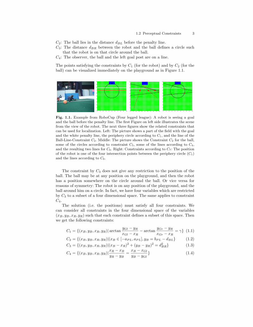
We start with an example from RoboCup where the camera image of arobot shows a goal in front and the ball before the white line of the penaltyarea (Figure 1.1). It is not too difficult for a human interpreter to give anestimate for the position (xB , yB) of the ball and the position (xR, yR) of theobserving robot. Humans can do that, regarding relations between objects,like the estimated distance dBR between the robot and the ball, and by theirknowledge about the world, like the positions of the goalposts and of thepenalty line.

The program of the robot can use the related features using image process-ing. The distance dBR can be calculated from the size of the ball in the image,or from the angle of the camera. The distance dBL between the ball and thepenalty line can be calculated, too. Other values are known parameters of theenvironment: (xGl, yGl), (xGr, yGr) are the coordinates of the goalposts, andthe penalty line is given as the set of points {(x, bPL)| − aPL ≤ x ≤ aPL}.The coordinate system has its origins at the center point, the y-axis points tothe observed goal.

The relations between the objects can be described by constraints. Thefollowing four constraints are obvious by looking to the image, and they canbe determined by the program of the observing robot:

C1: The view angle γ between the goalposts (the distance between them inthe image) defines a circle (periphery circle).

1.2 Perceptual Constraints 3

C2: The ball lies in the distance dBL before the penalty line.C3: The distance dBR between the robot and the ball defines a circle such

that the robot is on that circle around the ball.C4: The observer, the ball and the left goal post are on a line.

The points satisfying the constraints by C1 (for the robot) and by C2 (for theball) can be visualized immediately on the playground as in Figure 1.1.

0 10 20 30 40 50 60 70 80 90 1000

10

20

30

40

50

60

70

80

90

100

0 10 20 30 40 50 60 70 80 90 1000

10

20

30

40

50

60

70

80

90

100

0 10 20 30 40 50 60 70 80 90 1000

10

20

30

40

50

60

70

80

90

100

Fig. 1.1. Example from RoboCup (Four legged league): A robot is seeing a goaland the ball before the penalty line. The first Figure on left side illustrates the scenefrom the view of the robot. The next three figures show the related constraints thatcan be used for localization. Left: The picture shows a part of the field with the goaland the white penalty line, the periphery circle according to C1, and the line of theBall-Line-Constraint C2. Middle: The picture shows the Constraint C2 for the ball,some of the circles according to constraint C5, some of the lines according to C4,and the resulting two lines for C6. Right: Constraints according to C7: The positionof the robot is one of the four intersection points between the periphery circle (C1)and the lines according to C6.

The constraint by C3 does not give any restriction to the position of theball. The ball may be at any position on the playground, and then the robothas a position somewhere on the circle around the ball. Or vice versa forreasons of symmetry: The robot is on any position of the playground, and theball around him on a circle. In fact, we have four variables which are restrictedby C3 to a subset of a four dimensional space. The same applies to constraintC4.

The solution (i.e. the positions) must satisfy all four constraints. Wecan consider all constraints in the four dimensional space of the variables(xB , yB , xR, yR) such that each constraint defines a subset of this space. Thenwe get the following constraints:

C1 = {(xB , yB , xR, yR)| arctanyGl − yRxGl − xR

− arctanyGr − yRxGr − xR

= γ} (1.1)

C2 = {(xB , yB , xR, yR)|(xB ∈ [−aPL, aPL], yB = bPL − dBL} (1.2)

C3 = {(xB , yB , xR, yR)|(xB − xR)2 + (yB − yR)2 = d2BR} (1.3)

C4 = {(xB , yB , xR, yR)|xR − xByR − yB

=xB − xGl

yB − yGl} (1.4)

4 Daniel Gohring, Heinrich Mellmann, Hans-Dieter Burkhard

Then the possible solutions (as far as determined by C1 to C4) are givenby the intersection

⋂1,...,4 Ci. According to this fact, we can consider more

constraints C5, . . . , Cn as far as they do not change this intersection, i.e. asfar as

⋂1,...,n Ci =

⋂1,...,4 Ci . Especially, we can combine some of the given

constraints.By combining C2 and C3 we get the constraint C5 = C2 ∩ C3 where the

ball position is restricted to any position on the penalty line, and the playeris located on a circle around the ball. Then, by combining C4 and C5 we getthe constraint C6 = C4 ∩ C5 which restricts the positions of the robot to thetwo lines shown in Figure 1.1 (middle).

Now intersecting C1 and C6 we get the constraint C7 with four intersectionpoints as shown in Figure 1.1 (right). According to the original constraintsC1 to C4, these four points are determined as possible positions of the robot.The corresponding ball positions are then given by C2 and C4.

1.3 Formal Definitions of Constraints

We define all constraints over the set of all variables v(1), v(2), ..., v(k) (evenif some of the variables are not affected by a constraint). The domain of avariable v is denoted by Dom(v), and the whole universe under considerationis given by

U = Dom(v(1))× · · · ×Dom(v(k))

For this paper, we will consider all domains Dom(v) as (may be infinite)intervals of real numbers, i.e. U ⊆ Rk.

Definition 1. (Constraints)

1. A constraint C over v(1), ..., v(k) is a subset C ⊆ U .2. An assignment β of values to the variables v(1), ..., v(k), i.e. β ∈ U , is a

solution of C iff β ∈ C.

Definition 2. (Constraint Sets)

1. A constraint set C over v(1), ..., v(k)is a finite set of constraints overthose variables: C = {C1, ..., Cn}.

2. An assignment β ∈ U is a solution of C if β is a solution of all C ∈ C,i.e. if β ∈

⋂C

3. A constraint set C is inconsistent if there is no solution, i.e. if⋂C = ∅

The problem of finding solutions is usually denoted as solving a constraintsatisfaction problem (CSP) which is given by a constraint set C. By our def-inition, a solution is a point of the universe U , i.e. an assignment of valuesto all variables. For navigation problems it might be possible that only somevariables are of interest. This would be the case if we are interested only inthe position of the robot in our example above. Nevertheless we had to solvethe whole problem to find a solution.

1.4 Constraint Propagation 5

In case of robot navigation, there is always a unique solution of the prob-lem in reality (the positions in the real scene). This has an impact on theinterpretation of solutions and inconsistencies of the constraint system (cf.Section 1.4).

The constraints are models of relations (restrictions) between objects inthe scene. The information is derived from sensory data, from communicationwith other robots, or from knowledge about the world – as in the examplefrom above. Since information may be noisy, the constraints may not be asstrict as in the introductory example from Section 1.2. Instead of a circle weget an annulus for the positions of the robot around the ball according toC3 in the example. In general, a constraint may concern a subspace of anydimension (e.g. the whole penalty area, the possible positions of an occludedobject, etc.). Moreover, constraints need not to be connected: If there areindistinguishable landmarks, then the distance to such landmarks defines aconstraint consisting of several circles.

Other constraints are given by velocities: Changes of locations are re-stricted by the direction and speed of objects. This means that a positioncannot change too much within a short time.

There are many redundancies which are due to all available constraints. Vi-sual information in images usually contain lots of useful information: Size andappearance of observed objects, bearing angles, distances and other relationsbetween observed objects, etc. Only a very small part of this information isusually used in classical localization algorithms. This might have originated inthe fact, that these algorithms have been developed for range measurements.Another problem is the large amount of necessary calculation for Bayesianmethods (grids, particles). Kalman filters can process such large amounts, butthey rely on additional presumptions according to the underlying statistics.

Like Kalman filters, the constraint approach has the advantage, that itcan simultaneously compute positions of different objects and the relationsbetween them. Particle filters can deal only with small dimensions of searchspaces.

For constraint methods, we have the problem of inconsistencies. Accordingto the noise of measurements, it may be impossible to find a position whichis consistent with all constraints. In our formalism the intersection of all con-straints will be empty in such a case. Inconsistency in constraint satisfactionproblems means usually that there does not exist a solution in reality. But inour situation, the robot (and the other objects) do have their coordinates, onlythe sensor noise corrupted the data. Related quality measures for constraintsets have been investigated in [4].

1.4 Constraint Propagation

Known techniques (cf. e.g. [5] [6]) for constraint problems produce successivelyreduced sets leading to a sequence of decreasing restrictions

6 Daniel Gohring, Heinrich Mellmann, Hans-Dieter Burkhard

U = D0 ⊇ D1 ⊇ D2,⊇ . . .

Restrictions for numerical constraints are often considered in the form ofk-dimensional intervals I = [a,b] := {x|a ≤ x ≤ b} where a,b ∈ U and the≤-relation is defined componentwise. The set of all intervals in U is denotedby I. A basic scheme for constraint propagation with

• A constraint set C = {C1, ..., Cn} over variables v(1), ..., v(k) with domainU = Dom(v(1))× ...×Dom(v(k)).

• A selection function c : N→ C which selects a constraint C for processingin each step i.

• A propagation function d : 2U ×C → 2U for constraint propagation whichis monotonously decreasing in the first argument: d(D,C) ⊆ D.

• A stop function t : N→ {true, false}.

works as follows:

Definition 3. (Basic Scheme for Constraint Propagation, BSCP)

Step(0) Initialization: D0 := U , i := 1Step(i) Propagation: Di := d(Di−1, c(i)).

If t(i) = true: Stop.Otherwise i := i+ 1, continue with Step(i).

We call any algorithm which is defined accordingly to this scheme a BSCP-algorithm.

The restrictions are used to shrink the search space for possible solutions. If theshrinkage is too strong, possible solutions may be lost. For that, backtrackingis allowed in related algorithms.

To keep the scheme simple, the functions c and t depend only on thetime step. A basic strategy for c is a round robin over all constraints fromC, while more elaborate algorithms use some heuristics. A more sophisticatedstop criterion t considers the changes in the sets Di. Note that the sequenceneeds not to become stationary if only Di = Di−1. Actually, the sequenceD0, D1, D2, . . . needs not to become stationary at all.

For localization problems with simple constraints it is possible to computethe solution directly:

Corollary 1. If the propagation function d is defined by d(D,C) := D ∩ Cfor all D ⊆ U and all C ∈ C, then the sequence becomes stationary aftern = card(C) steps with the correct result Dn =

⋂C.

For simpler calculations, the restrictions Di are often taken in simpler forms(e.g. as intervals) and the restriction function d is defined accordingly.

Usually constraint satisfaction problems need only some but not necessar-ily all solutions. For that, the restriction function d does not need to regardall possible solutions (i.e. it need not be conservative according to definition5 below). A commonly used condition is local consistency:

1.4 Constraint Propagation 7

Definition 4. (Locally consistent propagation function)

1. A restriction D is called locally consistent w.r.t. a constraint C if

∀d = [d1, ..., dk] ∈ D ∀i = 1, ..., k ∃d′ = [d′1, ..., d′k] ∈ D ∩ C : di = d′i

i.e. if each value of a variable of an assignment from D can be completedto an assignment in D which satisfies C.

2. A propagation function d : 2U × C → 2U is locally consistent if it holdsfor all D, C: d(D,C) is locally consistent for C.

3. The maximal locally consistent propagation function dmaxlc : 2U×C →2U is defined by dmaxlc(D,C) := Max{d(D,C)|d is locally consistent}.

Since the search for solutions is easier in a more restricted the searchspace (as provided by smaller restrictions Di), constraint propagation is oftenperformed not with dmaxlc, but with more restrictive ones. Backtracking toother restrictions is used if no solution is found.

For localization tasks, the situations is different: We want to have anoverview about all possible poses. Furthermore, if a classical constraint prob-lem is inconsistent, then the problem has no solution. In localization problem,there does exist a solution in reality (the real poses of the objects under con-sideration). The inconsistency is caused e.g. by noisy sensory data. For that,some constraints must be relaxed or enlarged in the case of inconsistencies.This can be done during the propagation process by the choice of even a largerrestrictions than given by the maximal locally consistent restriction function.

Definition 5. (Conservative propagation function)A propagation function d : 2U×C → 2U is called conservative if D∩C ⊆

d(D,C) for all D and C.

Note that the maximal locally consistent restriction function dmaxlc isconservative. We have:

Proposition 1. Let the propagation function d be conservative.

1. Then it holds for all restrictions Di :⋂C ⊆ Di.

2. If any restriction Di is empty, then there exists no solution, i.e.⋂C = ∅.

If no solution can be found, then the constraint set is inconsistent. Thereexist different strategies to deal with that:

• enlargement of some constraints from C,• usage of only some constraints from C,• computation of the best fitting hypothesis according to C.

We have discussed such possibilities in the paper [4].As already mentioned above, intervals are often used for the restrictions

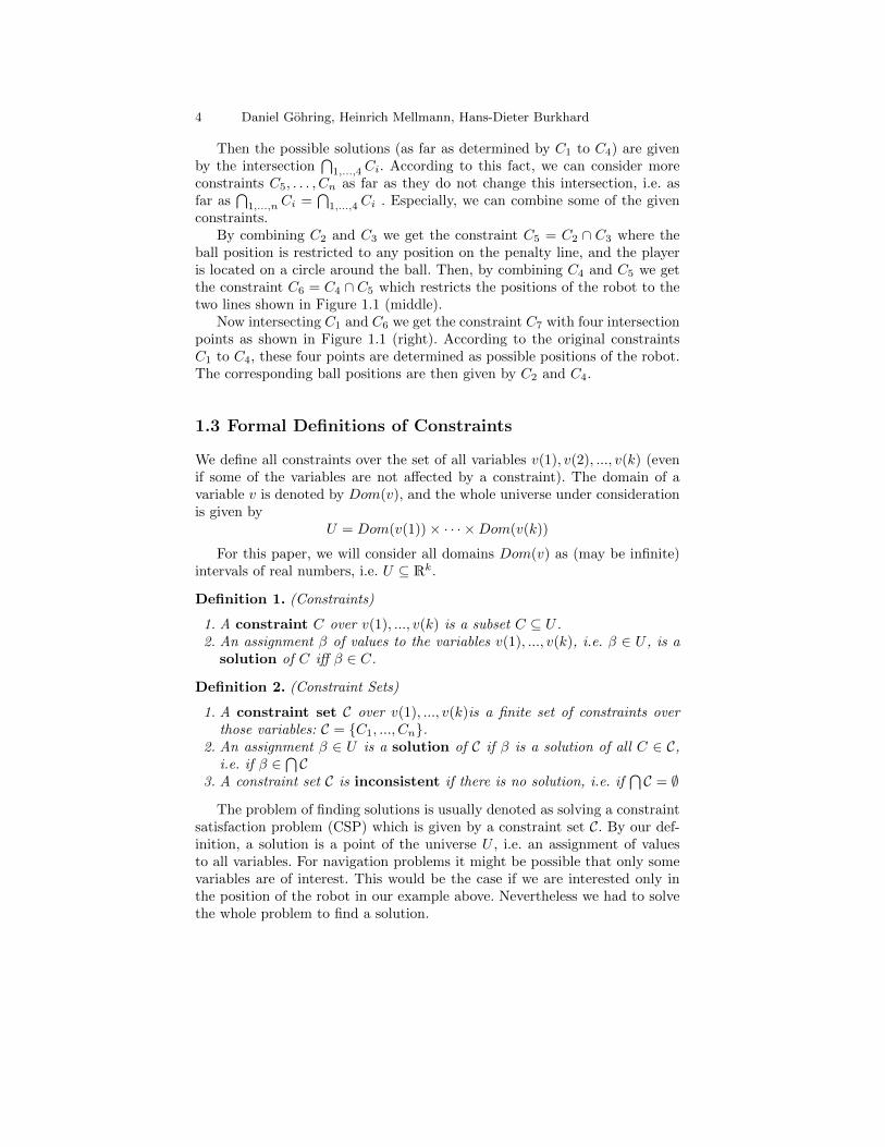
D, since the computations are much easier. Constraints are intersected withintervals, and the smallest bounding interval can be used as a conservativeresult. Examples are given in Fig. 1.2.

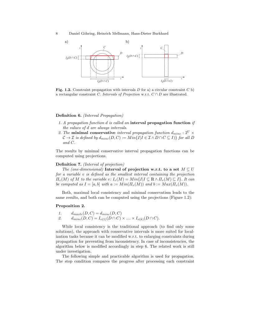
8 Daniel Gohring, Heinrich Mellmann, Hans-Dieter Burkhard

a) b)

x

y

Ix(D C)

Iy(D C)D

C

x

y

Ix(D C)

Iy(D C)D

C

Fig. 1.2. Constraint propagation with intervals D for a) a circular constraint C b)a rectangular constraint C. Intervals of Projection w.r.t. C ∩D are illustrated.

Definition 6. (Interval Propagation)

1. A propagation function d is called an interval propagation function ifthe values of d are always intervals.

2. The minimal conservative interval propagation function dminc : 2U ×C → I is defined by dminc(D,C) := Min{I|I ∈ I ∧D∩C ⊆ I)} for all Dand C.

The results by minimal conservative interval propagation functions can becomputed using projections.

Definition 7. (Interval of projection)The (one-dimensional) Interval of projection w.r.t. to a set M ⊆ U

for a variable v is defined as the smallest interval containing the projectionΠv(M) of M to the variable v: Iv(M) = Min{I|I ⊆ R∧Πv(M) ⊆ I}. It canbe computed as I = [a, b] with a := Min(Πv(M)) and b := Max(Πv(M)).

Both, maximal local consistency and minimal conservatism leads to thesame results, and both can be computed using the projections (Figure 1.2):

Proposition 2.

1. dmaxlc(D,C) = dminc(D,C)2. dminc(D,C) = Iv(1)(D ∩ C)× ....× Iv(k)(D ∩ C).

While local consistency is the traditional approach (to find only somesolutions), the approach with conservative intervals is more suited for local-ization tasks because it can be modified w.r.t. to enlarging constraints duringpropagation for preventing from inconsistency. In case of inconsistencies, thealgorithm below is modified accordingly in step 6. The related work is stillunder investigation.

The following simple and practicable algorithm is used for propagation.The stop condition compares the progress after processing each constraint

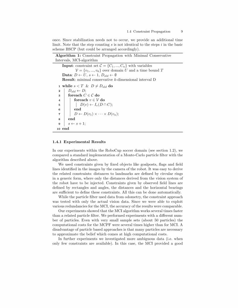
1.4 Constraint Propagation 9

once. Since stabilization needs not to occur, we provide an additional timelimit. Note that the step counting s is not identical to the steps i in the basicscheme BSCP (but could be arranged accordingly).

Algorithm 1: Constraint Propagation with Minimal ConservativeIntervals, MCI-algorithm

Input: constraint set C = {C1, ..., Cn} with variablesV = {v1, ..., vk} over domain U and a time bound T

Data: D ← U , s← 1, Dold ← ∅Result: minimal conservative k-dimensional interval D

1 while s < T & D 6= Dold do2 Dold ← D;3 foreach C ∈ C do4 foreach v ∈ V do5 D(v)← Iv(D ∩ C);6 end7 D ← D(v1)× · · · ×D(vn);

8 end9 s← s+ 1;

10 end

1.4.1 Experimental Results

In our experiments within the RoboCup soccer domain (see section 1.2), wecompared a standard implementation of a Monte-Carlo particle filter with thealgorithm described above.

We used constraints given by fixed objects like goalposts, flags and fieldlines identified in the images by the camera of the robot. It was easy to derivethe related constraints: distances to landmarks are defined by circular ringsin a generic form, where only the distances derived from the vision system ofthe robot have to be injected. Constraints given by observed field lines aredefined by rectangles and angles, the distances and the horizontal bearingsare sufficient to define these constraints. All this can be done automatically.

While the particle filter used data from odometry, the constraint approachwas tested with only the actual vision data. Since we were able to exploitvarious redundancies for the MCI, the accuracy of the results were comparable.

Our experiments showed that the MCI algorithm works several times fasterthan a related particle filter. We performed experiments with a different num-ber of particles. Even with very small sample sets (about 50 particles) thecomputational costs for the MCPF were several times higher than for MCI. Adisadvantage of particle based approaches is that many particles are necessaryto approximate the belief which comes at high computational costs.

In further experiments we investigated more ambiguous data (i.e. whenonly few constraints are available). In this case, the MCI provided a good

10 Daniel Gohring, Heinrich Mellmann, Hans-Dieter Burkhard

estimation of all possible positions (all those positions which are consistentwith the vision data). The handling of such cases is difficult for MCPF becausemany particles would be necessary. Related situations may appear for sparsesensor data and for the kidnapped robot problem. Odometry can improve theresults in case of sparse data (for MCPF as well as with additional constraintsin MCI). But we would argue that the treatment of true ambiguity by MCIis better for the kidnapped robot problem.

1.5 Conclusion

Constraint propagation techniques are an interesting alternative to probabilis-tic approaches. From a theoretical point of view, they could help for betterunderstanding of navigation tasks at all. For practical applications they per-mit the investigation of larger search spaces employing the constraints betweenvarious data. Therewith, the many redundancies in images can be better used.This paper has shown how sensor data can be transformed into constraints.We presented an algorithm for constraint propagation and discussed somedifferences to classical constraint solving techniques. In our experiments, thealgorithm outperformed classical approaches like particle filters.

The different strategies for dealing with inconsistencies have to be inves-tigated in more detail. This will be done by connecting the results from thispaper with our results from [4]. In further work we will analyze constraintbased approaches for cooperative object modeling tasks as well as very dy-namic situations with quickly changing object states.

References

1. Gutmann, J.S., Burgard, W., Fox, D., Konolige, K.: An experimental comparisonof localization methods. In: Proceedings of the 1998 IEEE/RSJ InternationalConference on Intelligent Robots and Systems (IROS), IEEE (1998)

2. Kalman, R.: A new approach to linear filtering and prediction problems. Trans-actions of the ASME - Journal of Basic Engineering 82 (1960) 35–45

3. Jungel, M.: Memory-based localization. (2007) Proceedings of the CS&P 2007.4. Gohring, D., Gerasymova, K., Burkhard, H.D.: Constraint based world modeling

for autonomous robots. (2007) Proceedings of the CS&P 2007.5. Davis, E.: Constraint propagation with interval labels. Artificial Intelligence 32

(1987)6. Goualard, F., Granvilliers, L.: Controlled propagation in continuous numerical

constraint networks. ACM Symposium on Applied Computing (2005)