Constructing invariants for hybrid systems

Constructing Invariants for Hybrid Systems ∗

Sriram Sankaranarayanan, Henny B. Sipma and Zohar MannaComputer Science Department, Stanford University, Stanford, CA 94305, USA

Abstract. We present a new method for generating algebraic invariants of hy-brid systems. The method reduces the invariant generation problem to a constraintsolving problem using techniques from the theory of ideals over polynomial rings.Starting with a template invariant – a polynomial equality over the system variableswith unknown coefficients – constraints are generated on the coefficients guaran-teeing that the solutions are inductive invariants. To control the complexity of theconstraint solving, several stronger conditions that imply inductiveness are proposed,thus allowing a trade-off between the complexity of the invariant generation processand the strength of the resulting invariants.

1. Introduction

Hybrid systems are reactive systems that combine discrete mode changeswith the continuous evolution of the system variables, specified in theform of differential equations. The analysis of hybrid systems is an im-portant problem that has been studied extensively both by the controltheory, and the formal verification community for over a decade. Amongthe most important analysis questions for hybrid systems are those ofsafety, i.e, deciding whether a given property ψ holds in all the reach-able states, and the dual problem of reachability, i.e, deciding if a statesatisfying the given property ψ is reachable. Both these problems arecomputationally hard — intractable even for the simplest subclasses,and undecidable for the general case.

In this paper, we provide techniques to generate invariants for hy-brid systems. An invariant of a hybrid system is a property ψ thatholds in all the reachable states of the system. An inductive assertionof a hybrid system is an assertion ψ that holds at the initial statesof the system, and is preserved by all discrete and continuous statechanges. Therefore, any inductive assertion is also an invariant asser-tion. Furthermore, the standard technique for proving a given assertionϕ invariant is to generate an inductive assertion ψ that implies ϕ.Therefore, the problem of invariant generation is also one of inductiveassertion generation. This problem has received wide attention in the

∗ This research was supported in part by NSF grants CCR-01-21403, CCR-02-20134 and CCR-02-09237, by ARO grant DAAD19-01-1-0723, by ARPA/AFcontracts F33615-00-C-1693 and F33615-99-C-3014, and by NAVY/ONR contractN00014-03-1-0939.

c© 2005 Kluwer Academic Publishers. Printed in the Netherlands.

differential.tex; 18/02/2005; 9:15; p.1

2

program analysis community [18, 9, 10, 34, 28, 8, 4]. The generation oflinear inductive assertions for the special case of linear hybrid systemshas also been studied [14]. Many other approaches that compute theexact or the approximate reach-set of a given hybrid system can alsobe shown to compute inductive assertions [15, 32, 19].

In this paper, we extend our previous work on non-linear inductiveassertion generation [28] for discrete systems to generate invariants forhybrid systems. We use the theory of ideals over polynomials alongwith standard computational techniques in algebraic geometry involv-ing Grobner bases to provide a technique for computing inductiveassertions for hybrid systems.

The key idea behind our technique is that given a template asser-tion, i.e, a parametric polynomial with unknown coefficients and ofbounded degree in the system variables, we derive constraints on theunknown coefficients so that any solution to these constraints is aninductive assertion. To keep these constraints tractable, we considerseveral useful restrictions on the nature of an invariant. In particular,we consider stronger conditions for inductiveness than the traditionalrequirements [20]. Also, we provide conceptually simpler techniquesto handle the continuous evolution; these techniques require neither aclosed form solution to the differential equations nor an approximationthereof.

Our technique can construct inductive assertions using less time andspace than traditional techniques. Depending on the nature of the con-secution condition chosen, our constraint generation technique is linearin the number of modes and discrete transitions, and polynomial in thenumber of system variables. Furthermore, the constraints generated canrange in complexity from the more intractable non-linear constraintsrequiring quantifier elimination to simple constraints involving onlylinear equalities. Of course, the more complex constraints potentiallyyield stronger invariants than the simpler constraints. This trade-off isuseful in practice, and contributes to making the method scale.

Related Work

The verification of safety (invariance and reachability) properties oftimed and hybrid automata has been the subject of numerous papers,and has lead to popular verification systems such as Kronos [36],Uppaal [3], Hytech [17], d/dt [1], and CheckMate [31]. Most ofthis work deals with hybrid systems with piecewise-linear dynamics,although some tools, notably CheckMate, can handle more generaldynamics. Non-linear systems have been traditionally dealt with byusing finite-state, or linear infinite-state abstractions [15]. Techniques


3

using template properties with undetermined coefficients along withconstraint solving have appeared intermittently both in the computerscience, and the control theory literature. Techniques for automaticgeneration of linear equality invariants for Petri-nets are a classic ex-ample [23]. Our earlier work on discrete linear systems handles thegeneration of linear inequality invariants using Farkas’ Lemma [8, 29].The work of Forsman et al. [12] uses Grobner bases and parameterizedpolynomials to construct Lyapunov functions to prove local stabilityof continuous systems. Their approach works by fixing the form ofthe desired Lyapunov function, and computing a maximal region overwhich a function of the given form can establish local stability.

Invariant-generation methods for discrete programs based on al-gebraic geometry have appeared recently. The work of Muller-Olmand Seidl, presents a backward propagation-based method for non-linear programs without branch conditions [22]. In [7], Colon presentsa method that uses forward propagation in the lattice of pseudo idealsof a given degree, to generate invariants of a bounded degree. In [27],Rodriguez-Carbonell and Kapur present a method to generate poly-nomial invariants for programs that contain only a special class ofassignments called solvable assignments. In [26], a forward-propagation-based technique is presented, in which statements are represented astransformations on ideals. A widening operator that limits invariantsto a given degree is used.

The work of Parillo et al. [24] presents a powerful framework basedon real-algebraic geometry and semi-definite programming. Conceptu-ally, this framework can be made to play the same role as that ofGrobner bases in this work. This has already been applied to someaspects of the safety-verification problem by the recent work of Prajnaand Jadbabaie using the idea of barrier certificates [25]. Ideas similarto the ones contained in this work have appeared independently in thework of Tiwari and Khanna [33].

The rest of the paper is organized as follows: Section 2 presents ourcomputational model and the basic theory behind ideals and Grobnerbases. Section 3 presents the constraint generation process. The na-ture of these constraints and their solution techniques are discussed inSection 4. In Section 5, we present some examples demonstrating theapplication of our techniques. Section 6 concludes with a discussion ofthe pros and cons.


4

2. Preliminaries

2.1. Computational Model: Hybrid Automata

To model hybrid systems we use hybrid automata [16].

Definition 1 (Hybrid System). A hybrid system Ψ: 〈V,L,T ,Θ,D, I, `0〉consists of the following components:

− V , a set of real-valued system variables. The number of variables(|V |) is called the dimension of the system. A state is an interpre-tation of V , assigning to each v ∈ V a real value. The set of allstates is denoted by Σ. An assertion is a first-order formula overV . A state s satisfies an assertion ϕ, written s |= ϕ, if ϕ holds ons. We will also write ϕ1 |= ϕ2 for two assertions ϕ1, ϕ2 to denotethat ϕ2 is true at least in all the states in which ϕ1 is true.

− L, a finite set of locations;

− T , a set of (discrete) transitions. Each transition τ : 〈`1, `2, ρτ 〉 ∈T consists of a prelocation `1 ∈ L, a postlocation `2 ∈ L, and anassertion ρτ over V ∪V ′ representing the next-state relation, whereV ′ denotes the values of V in the next state;

− Θ, an assertion specifying the initial condition;

− D, a map that maps each location ` ∈ L to a differential rule(also known as a vector field or a flow field), D(`), of the formvi = fi(V ) for each vi ∈ V . The differential rule at a locationspecifies how the system variables evolve in that location.

− I, a map that maps each location ` ∈ L to a location condition(location invariant), I(`), an assertion over V ;

− `0 ∈ L, the initial location; we assume that the initial conditionsatisfies the location invariant at the initial location, that is, Θ |=I(`0).

Definition 2 (Computation). A computation of a hybrid system Ψis an infinite sequence of states 〈l, ~x〉 ∈ L ×R|V | of the form

〈l0, ~x0〉 , 〈l1, ~x1〉 , 〈l2, ~x2〉 , . . .

where ~xi are the values assigned to the variables in V , such that

Initiation: the initial state of the computation satisfies the initialcondition:

l0 = `0 and ~x0 |= Θ


5

l : y ≥ 0

y = vy

vy = −10

δ = 1

y = 0,δ > 0,v′y = −vy

2 ,y′ = yδ′ = 0,

τ

Figure 1. The hybrid automaton for a bouncing ball

Furthermore, for each consecutive state pair 〈li, ~xi〉, 〈li+1, ~xi+1〉, one ofthe two consecution conditions below is satisfied.

Discrete Consecution: there exists a transition τ : 〈`1, `2, ρτ 〉 ∈ Tsuch that li = `1, li+1 = `2, and 〈~xi, ~xi+1〉 |= ρτ , where theunprimed variables refer to ~xi and the primed variables to ~xi+1, or

Continuous Consecution: li = li+1 = `, and there exists a timeinterval δ > 0, along with a smooth (continuous and differentiableto all orders) function f : [0, δ] 7→ Rn, such that f evolves from~xi to ~xi+1 according to the differential rule at location `, whilesatisfying the location condition I(`). Formally,

1. f(0) = ~x1, f(δ) = ~x2, and (∀ t ∈ [0, δ]), f(t) |= I(`),

2. (∀t ∈ [0, δ)),⟨

f(t), f(t)⟩

|= D(`).

A state 〈`, ~x〉 is called a reachable state of a hybrid system Ψ if itappears in some computation of Ψ.

Example 1 (Bouncing Ball). Figure 1 shows a graphical represen-tation of the following hybrid system, representing a ball bouncing ona soft floor (y = 0):

V = {y, vy, δ}L = {l},T = {τ}, where, τ =

⟨

l, l,

[δ > 0 ∧ y = 0 ∧ y′ = y ∧v′y = −vy

2 ∧ δ′ = 0

]⟩

Θ = (y = 0 ∧ vy = 16 ∧ δ = 0)

D(l) =(

y = vy ∧ vy = −10 ∧ δ = 1)

I(l) = (y ≥ 0)`0 = l


6

The variable y represents the position of the ball, vy represents itsvelocity, and δ denotes the time elapsed since its last bounce. A bounceis modeled by the transition τ , in which the velocity vy of the ball ishalved, and the ball reverses direction.

Definition 3 (Invariant). An invariant of a hybrid system Ψ at alocation ` is an assertion ψ such that for any reachable state 〈`, ~x〉 ofΨ, ~x |= ψ.

Definition 4 (Inductive Assertion Map). An inductive assertionmap Ψ is a map that associates with each location ` ∈ L an assertionΨ(`) that holds initially and is preserved by all discrete transitions andcontinuous flows. More formally an inductive assertion map satisfiesthe following requirements:

Initiation Θ |= Ψ(`0),

Discrete Consecution For each discrete transition τ : 〈`1, `2, ρ〉,starting from a state satisfying Ψ(`1), and taking τ leads to astate satisfying Ψ(`2). Formally,

Ψ(`1) ∧ ρτ |= Ψ(`2)′

where Ψ(`2)′ represents the assertion Ψ(`2) with the current state

variables ~x replaced by the next state variables ~x′.

Continuous Consecution For every location ` ∈ L, and states 〈`, ~x1〉,〈`, ~x2〉 such that ~x2 evolves from ~x1 according to the differentialrule D(`) at `, if ~x1 |= Ψ(`) then ~x2 |= Ψ(`). If Ψ(`) is an assertionof the form f`(~x) = 0, for a real-valued smooth function f`, we canexpress consecution by the condition

I(`)(~x) ∧ (f`(~x) = 0) |= f`(~x) = 0 .

Note that f` denotes the Lie-derivative of f` along the vector fieldD(`). The condition above is important, since we shall only beinterested in inductive assertions of the form p = 0 for a polynomialp.

An assertion ϕ is inductive if the assertion map that maps eachlocation to ϕ is an inductive assertion map. It is easy to see that aninductive assertion is an invariant. However, an invariant assertion isnot necessarily inductive.

Example 2. For the hybrid system in Example 1, the assertion y =vyδ − 5δ2 is an inductive and invariant assertion. It can be shown tosatisfy all the requisite conditions for being inductive. On the otherhand, the assertion vy ≤ 16 is an invariant but not inductive. This isbecause, it does not satisfy consecution for the discrete transition τ .


7

2.2. Algebraic Assertions and Ideals

We begin by presenting some definitions and results from commutativealgebra. Informally, an ideal is a set of equations between polynomialsalong with all their consequences. Ideals can be used to deduce factsabout the set of points that satisfy their underlying equations. Some ofthe results in this section are stated in general terms without proofs.Details can be found in most standard texts on algebra and algebraicgeometry [11, 21].

Let R be the set of reals and C be the set of complex numbersobtained as the algebraic closure of the reals. Let V = {x1, . . . , xn} bea set of variables. The set of polynomials on V , with coefficients fromR (C) is denoted by R[x1, . . . , xn] (C[x1, . . . , xn]).

Definition 5 (Algebraic Assertion). An algebraic assertion ψ is afinite conjunction of polynomial equations denoted by

∧

i

pi(x1, . . . , xn) = 0,

where each pi ∈ R[x1, . . . , xn]. The degree of an assertion is the maxi-mum among the degrees of the polynomials that make up the assertion.

Definition 6 (Algebraic Hybrid Systems). An algebraic hybridsystem is a hybrid system Ψ : 〈V,L,T ,Θ,D, I, `0〉, where,

1. For each transition τ : 〈`1, `2, ρτ 〉 ∈ T , the relation ρτ is analgebraic assertion,

2. The initial condition Θ, and the location conditions I(`) are alsoalgebraic assertions, and

3. Each rule D(`) is of the form∧

i xi = pi(x1, . . . , xn).

Definition 7 (Variety). A variety is the set of points in the com-plex plane that satisfy an algebraic assertion. Given an assertion ψ :∧

i(pi(~x) = 0), its corresponding variety is defined as

Variety(ψ) = {~z ∈ Cn | (∀i) pi(~z) = 0}.

Definition 8 (Ideal). A set I ⊆ R[x1, . . . , xn] is an ideal, if

1. 0 ∈ I,

2. If p1, p2 ∈ I then p1 + p2 ∈ I,

3. If p1 ∈ I and p2 ∈ R[x1, . . . , xn] then p1p2 ∈ I.


8

An ideal generated by a set of polynomials P , denoted by ((P )), isthe smallest ideal containing P . Equivalently,

((P )) =

{

g1p1 + · · · + gmpm | g1, . . . , gm ∈ R[x1, · · · , xn],p1, . . . , pm ∈ P

}

.

An ideal I is finitely generated if there is a finite set P such thatI = ((P )). A famous theorem due to Hilbert states that all ideals inR[x1, . . . , xn] are finitely generated. As a result, algebraic assertions canbe seen as the generators of an ideal and vice-versa. Any ideal definesa variety, which is the set of the common zeroes of all the polynomialsit contains. This correspondence between ideals and varieties is one ofthe fundamental observations involving algebraic assertions called theHilbert’s Nullstellensatz. We state the relevant direction of this theorembelow:

Theorem 1 (Hilbert’s Nullstellensatz). Consider an algebraicassertion ψ. Let I = ((ψ)) be the ideal generated by ψ in R[x1, . . . , xn],and f(x1, . . . , xn) ∈ R[x1, . . . , xn]. If f ∈ I, then

(∀~z ∈ Cn) ψ(~z) ⇒ (f(~z) = 0)

i.e, ψ(~x) |= (f(~x) = 0).

Proof. Let ψ ≡ f1 = 0 ∧ · · · ∧ fm = 0 and f ∈ I. Hence, we canexpress f as

f = g1f1 + · · · + gmfm

for some g1, . . . , gm ∈ R[x1, . . . , xn]. Let ~z ∈ Cn be such that ψ(~z)holds. Then, f(~z) =

∑mi=1(gi(~z)fi(~z)) = 0, since each fi(~z) = 0, and

therefore(∀~z ∈ Cn) ψ(~z) ⇒ (f(~z) = 0).

The theorem shows that membership of a polynomial p in an idealI leads to the semantic entailment of p = 0 by the variety induced byI. Hence, an ideal is (informally) a Consequence-Closed set of polyno-mials. While a similar statement can be made in the converse, it is notrelevant to the soundness of our technique, and therefore we omit itfrom the discussion. Note that even though the ideals are defined inR[x1, . . . , xn], the varieties along with the entailments are defined overthe complex numbers, which subsume the reals. This is a technicalitythat arises from the fact that the reals are not algebraically closed.

Remark. Figure 2 shows an instructive comparison between the de-duction of consequences of linear equalities and that of polynomial


9

Linear Equalities Polynomial Equalities

Hyperplanes Varieties

λ1 e1 = 0...

...

λm em = 0

e = 0

g1 p1 = 0...

...

gm pm = 0

p = 0

e = λ1e1 + · · · + λmem p = g1p1 + · · · + gmpm

e ∈ linear(e1, . . . , em) p ∈ ((p1, . . . , pm))

Figure 2. Comparison between multivariate linear equations and multivariatepolynomial equations

equalities, ignoring some technical details. A given set of linear equal-ities, e1 = 0, . . . , em = 0, entails a new linear equality e = 0 iff e canbe written as a linear combination of e1, . . . , em. The set of all linearcombinations of e1, . . . , em, forms a linear subspace. Similarly, for thepolynomial equalities, the real multipliers λ1, . . . , λm, are replaced byarbitrary polynomials g1, . . . , gm. The set of all such combinations ofp1, . . . , pm, is the ideal generated by p1, . . . , pm.

Example 3. The assertion ψ = (p1 : x2 + 2x + y2 − 1 = 0 ∧ p2 :x2−2x+y2−1 = 0) represents the intersection of two circles each withradius

√2, centered at (−1, 0) and (1, 0), respectively. They intersect

at two points (0, 1) and (0,−1). Furthermore, x = p1−p2

4 , and hencex ∈ ((p1, p2)). Geometrically, this states that p1 = 0 ∧ p2 = 0 |= x = 0,or in other words all the points of intersection of the two circles lie onthe y-axis. Also, x2 + y2 − 1 = p1+p2

2 ∈ ((p1, p2)). Therefore, we candeduce that the points satisfying ψ also lie on the circle with radius 1centered at the origin.

In the remainder of this subsection, we use the concept of ideals toderive a systematic algorithm for determining, given an assertion ψ anda polynomial f , whether f ∈ ((ψ)). We assume that all the polynomialsare drawn from R[x1, . . . , xn], and all consequence relations of the formψ1 |= ψ2 are over the domain of complex numbers.

Let V = {x1, . . . , xn} be a set of variables. A monomial over V is ofthe form xr1

1 xr2

2 · · · xrnn , with ri ∈ N . The set of monomials is denoted

by M . A term is of the form c · p where c ∈ R and p ∈ M . The set ofterms is denoted by Term.


10

Definition 9 (Monomial Orderings). A monomial ordering < is atotal and strict ordering on M that satisfies the following properties:

1. (∀t ∈ M ) 1 ≤ t,

2. If (t1 ≤ t2) then (∀t ∈ M ) t1t ≤ t2t.

These orderings can be extended to a non-total ordering over terms byignoring the coefficients.

Monomial orderings are used to induce a reduction relation overpolynomials. Many monomial orderings appear in the literature, themost common being the lexicographic and total-degree lexicographicorderings. Assuming a linear ordering ≺ on the variables in V , x1 ≺x2 ≺ · · · ≺ xn, the lexicographic extension ≺lex is defined as:

xr1

1 · · · xrnn ≺lex x

q1

1 · · · xqnn iff (∃i) ri < qi ∧ (∀ j < i) rj = qj.

The ordering is lexicographic on the tuple 〈r1, . . . , rn〉 corresponding toa term xr1

1 · · · xrnn . The total-degree lexicographic ordering is a variant of

this order: it first compares monomials by their total degree, defined asthe sum of the powers of all the variables, and then the lexicographicordering is used to resolve the tie for terms with the same total de-gree. In general, the choice of ordering affects the complexity of thealgorithms, but such an effect is not addressed in this paper.

Definition 10 (Lead term). Given a polynomial g, its lead term (de-noted lt(g)) is the largest term in g w.r.t. a given monomial ordering.

Definition 11 (Reduction). Let f, g be polynomials, and < be a

monomial ordering. The reduction relation over polynomials,g−→ is

defined as: fg−→ f ′ iff there exists term t in f s.t. lt(g) divides t, and

f ′ = f − t

lt(g)g.

The effect of the reduction is the cancellation of the term t thatwas selected. The reduction relation can be viewed as a term rewritingsystem over polynomials [2]. The reduction relation can be extended

to a finite set P of polynomials as fP−→ f ′ iff (∃g ∈ P ) f

g−→ f ′. The

reduction relationP−→ is terminating for any finite set of polynomials

P , as a direct consequence of the definition of monomial orderings. Anormal form f of the reduction relation is a polynomial such that nofurther reduction of f is possible. The reduction relation is confluent if

every polynomial reduces to a unique normal form. ByP�, we denote

the reflexive transitive closure of the relationP−→.


11

The reduction relation induced by P can be used to check member-ship of a given polynomial in the ideal generated by P :

Theorem 2 (Ideal Membership). Let I = ((P )) be an ideal, and f

be a polynomial. If fP� 0 then f ∈ I.

Proof. The proof proceeds by induction on the length of the derivation.

It is trivially true for zero length derivations, since 0 ∈ I. Let fP−→

f ′P� 0. It follows that f ′ = f − tg, for some suitable term t, and some

g ∈ P . Since f ′ ∈ I (the induction hypothesis), and g ∈ P , it followsthat f ′ + tg ∈ I. Thus, f ∈ I.

Example 4. Assume a set of variables x, y, z with a precedence order-ing x � y � z. Consider the ideal I = ((f : x2−y, g : y−z, h : x+z)),and the polynomial p : x2 − y2. Using the total lexicographic ordering,we have x2 > y, and thus the lead term in f is x2, which divides the

term t : x2 in p. Therefore, pf−→ p′, where

p′ = (x2 − y2)︸︷︷︸

p

−x2

x2︸︷︷︸

tlt(f)

(x2 − y)︸︷︷︸

f

= (−y2 + y).

The following sequence of reductions shows the membership of p in theideal

ph−→ −zx− y2 h−→ z2 − y2 g−→ −yz + z2 g−→ −z2 + z2 ≡ 0,

thus pI� 0, and hence p ∈ I. However, the reduction sequence

pf−→ −y2 + y

g−→ −yz + yg−→ −z2 + y

g−→ −z2 + z

reaches a normal-form without showing the ideal membership.

The reduction relationP−→ may not be confluent, as illustrated by

the example above. Therefore, Theorem 2 cannot be used to decidemembership of a polynomial in the ideal generated by P . Fortunately,for any ideal I = ((P )), there exists a special set of generators G

such that I = ((G)), and the reduction relationG−→ induced by G is

confluent. Such a basis for I is variously called the Grobner Basis, orthe Standard Basis of I.

Theorem 3 (Grobner Basis). Let I = ((P )) be an ideal, and f be

a polynomial. Let G be the Grobner basis of I. Then fG� 0 iff f ∈ I.


12

Proof. A proof of this theorem can be found in any standard text orsurvey on this topic [11, 21].

Since the reduction relation is terminating, Theorem 3 provides adecision procedure for ideal membership. We shall use nfG(p) to de-

note the normal form of a polynomial p underG�. The subscript G in

nfG(p) may be dropped if it is evident from the context. The standardalgorithm for computing the Grobner basis of an ideal is known asthe Buchberger algorithm. There are numerous implementations of thisalgorithm available with standard computer-algebra packages and poly-nomial computation libraries. As an example, the library groebnerimplements many improvements over the standard algorithm [35].

Example 5. Consider again the ideal from Example 4; I = ((f :x2 − y, g : y − z, h : x + z)). The Grobner basis for I is G = {f1 :z2−z, g : y−z, h : x+z}. With this basis, every reduction of p : x2−y2

will yield the normal form 0.

2.3. Templates

Our technique for invariant generation aims to find polynomials thatsatisfy certain properties. To represent these sets of polynomials we usetemplates — polynomials with coefficients that are linear expressionsover some set of template variables. We show that the theory of idealscan be naturally extended to templates. In particular, we show thatthere exist confluent reduction relations on templates that allow thegeneration of constraints on the template variables, such that the re-sulting set of polynomials is precisely the set of polynomials that belongto the desired ideal.

Definition 12 (Templates). Let A be a set of template variables andL(A) be the domain of all linear expressions over variables in A of theform c0 + c1a1 + . . .+ cnan, where each ci is a real-valued coefficient. Atemplate over A,V is a polynomial over variables in V with coefficientsfrom L(A).

Example 6. Let A = {a1, a2, a3}, and hence

L(A) = {c0 + c1a1 + c2a2 + c3a3 | c0, . . . , c3 ∈ R}.

The set of templates is the ring L(A)[x1, . . . , xn]. For example,

(2a2 + 3)x1x22 + (3a3)x2 + (4a3 + a1 + 10) ∈ L(A)[x1, . . . , xn].


13

Definition 13 (Semantics of Templates). Given a set of templatevariables A, an A-environment (if A is clear from the context, thensimply an environment) is a map α that assigns real values to eachvariable in A. This map is naturally extended to map expressions inL(A) to their corresponding values in R, and to map polynomials inL(A)[x1, . . . , xn] to their corresponding polynomials in R[x1, . . . , xn].

Example 7. The environment α ≡ 〈a1 = 0, a2 = 1, a3 = 2〉, maps thetemplate

(2a2 + 3)x1x22 + (3a3)x2 + (4a3 + a1 + 10)

from Example 6 to the polynomial

5x1x22 + 6x2 + 18.

The reduction relationg−→ for polynomials can be extended to a

reduction relation for templates in a natural way.

Definition 14 (Reduction of Templates). Let p be a polynomialin R[x1, . . . , xn] and f, f ′, be templates over A and {x1, . . . , xn}. The

reduction relation is defined as: fp−→ f ′ iff the lead term lt(p) divides

a term c · t in f with coefficient c(a0, . . . , am) and

f ′ = f − c · tlt(p)

p.

Remark. The reduction relation is a natural extension of the cor-responding reduction relation over polynomials. The definition abovedefines reductions of templates by polynomials in R[x1, . . . , xn]. Weshall not attempt to define reductions of templates by other templates.

The reduction relation can, in turn, be extended to sets of polyno-

mials to define reduction relationG−→ over templates for sets of poly-

nomials G. Henceforth, we shall use the symbols f, g, with subscriptsto denote templates and the symbols h, p, to denote polynomials.

Example 8. Let p be the polynomial x2−y, with lt(p) = x2. Considerthe template

f : ax2 + by2 + cz2 + dz + e.

The lead term lt(p) divides the term ax2 in f . Therefore, fp−→ f ′,

where

f ′ : (ax2 + by2 + cz2 + dz+ e)− ax2

x2(x2 − y) = by2 + cz2 + dz+ e+ ay.


14

Given a template f and an ideal I, the objective is to find thoseenvironments α such that α(f) ∈ I. This is achieved by obtainingconstraints on the environment variables A such that any solution αsatisfies α(f) ∈ I.

The properties of the Grobner basis reduction relations over poly-nomials can be extended smoothly to templates. Proofs of these resultscan be found in the appendix. We first show that the extension ofreduction relation is consistent w.r.t. the semantics of templates underany A-environment. The confluence of Grobner basis reduction relationover templates guarantees that a unique normal form exists for anytemplate (Theorem 8). The template membership theorem (Theorem10) proves that if f1 = nfG(f) is the normal form of f , then for eachenvironment α, α(f) ∈ ((G)) iff α(f1) is identically zero.

Theorem 4 (Zero Polynomial Theorem). A polynomial p is zerofor all the possible values of x1, . . . , xn iff all its coefficients are identi-cally zero.

Proof. The proof is available from any standard text on algebra.

Given a template f and an ideal I with Grobner basis G, we firstcompute nfG(f), and then equate each coefficient of the normal formto zero to obtain a set of equations over the template variables A. Anysolution to this set of equations yields an A-environment α such thatα(f) ∈ I (and conversely).

Example 9. Let I be the ideal ((x2 − y, y − z, z + x)) of Example 4with Grobner basis G = {x + z, y − z, z2 − z}. We are interested inpolynomials represented by the template

f : ax2 + by2 + cz2 + dz + e

that are members of the ideal. The normal form of this template is

nfG(f) : (a+ b+ c+ d)z + e .

Equating each coefficient in the normal form to zero, we obtain

a+ b+ c+ d = 0e = 0

From this, we can generate all instances of the template that belong toI. Some examples are x2−y2, y2− z, 2x2 − z2 − z. On the other hand,x2 + y2 − z 6∈ I, as the coefficients do not satisfy the constraints.


15

3. Constraint-Generation

Our invariant generation algorithm consists of the following steps:

1. fix a template map for the candidate invariant;

2. encode the conditions for invariance as an ideal-membership ques-tion;

3. derive the constraints on the template variables that guarantee theappropriate ideal-membership;

4. solve the constraints to obtain the invariants of the form specifiedby the template map.

In this section we describe and illustrate the first three steps; the laststep is presented in section 4.

3.1. Template Map

The first step in our method is to fix the shape of the desired invariants.Let A = {a1, a2, . . .} be a set of template variables, and let Ψ bean algebraic hybrid system with location set L = {`1, . . . , `m} andvariables V = {x1, . . . , xn}. A generic degree-k template over A and Vis the sum of all monomials of degree k or less, written as

∑

i1+···+in≤k

a〈i1,i2,...,in〉xi11 · · · xin

n

with a total of

(n+ kk

)

terms, and as many template variables. For

example, a degree-2 template for 5 variables has 21 terms.A template map η associates each location ` with a template. For

maximum generality, the template variables in the templates shouldbe all different. However, templates for different locations may havedifferent degree.

Example 10. For the system introduced in Example 1 we fix thetemplate map η as follows:

η(l) = a1y2 +a2v

2y +a3δ

2 +a4yvy +a5vyδ+a6yδ+a7y+a8vy +a9δ+a10

with the objective to identify the values of the coefficients a1 . . . a10 forwhich the assertion

a1y2 + a2v

2y + a3δ

2 + a4yvy + a5vyδ+ a6yδ+ a7y+ a8vy + a9δ+ a10 = 0

is an invariant at location l.


16

3.2. Encoding Invariance Conditions

The second step in our technique involves the encoding of the conditionsfor invariance as an ideal membership statement. Given a template η(`),we recast the invariance conditions as an ideal membership problem ofthe form

η(`) ∈ ((p1, . . . , pk))

where p1, . . . , pk, are polynomials over the reals. This is equivalent tonfG(η(`)) ≡ 0, where G is the Grobner basis of ((p1, . . . , pk)).

InitiationThe initiation condition, Θ |= (η(`0) = 0), is encoded by η(`0) ∈ ((Θ)).This is in turn encoded by computing the Grobner basis of Θ, andencoding nfΘ(η(`0)) ≡ 0.

Example 11. The initial condition for the bouncing ball example(Example 1) is (y = 0, vy = 16, δ = 0). Taking the template from Ex-ample 10, the normal form w.r.t. Θ is nf(η(l0)) = a10 + 256a2 + 16a8.Hence the constraint corresponding to initiation is a10+256a2 +16a8 =0.

Discrete ConsecutionThe consecution condition states that the invariant map must be pre-served by all transitions, i.e, for each transition 〈`1, `2, ρ〉,

(η(`1) = 0) ∧ ρ |= (η(`2)′ = 0)

must hold. Encoding this exactly would require the reduction of onetemplate (η(`2)) w.r.t. to another template (η(`1)). As noted in ourprevious work [28], this leads to complex constraints which are hardto solve in general. As an alternative we propose to use stronger con-ditions for consecution that imply the original consecution condition,but avoid the template in the antecedent. However, in doing so we losethe invariants that satisfy the general condition of consecution but notthe stronger conditions.

We describe four options for stronger consecution conditions, start-ing with the strongest. A summary of these conditions, together withtheir encodings, is shown in Figure 3.

Local Consecution (LC) The local consecution condition states thatthe transition simply establishes the invariant at the postlocation,without any assumptions on the precondition. Invariants that canbe established in this way are also known as local invariants orreaffirmed invariants.


17

Name Condition Encoding

lc ρ |= (η(l2)′ = 0) nfρ(η(l2)

′) ≡ 0

cv ρ |= (η(l1) = η(l2)′) nfρ(η(l1) − η(l2)

′) ≡ 0

cs (∃ λ) ρ |= (η(l2)′ = λη(l1)) (∃ λ) nfρ(η(l2)

′ − λη(l1)) ≡ 0

ps (∃ f) ρ |= (η(l2)′ = f · η(l1)) (∃ f) nfρ(η(l2)

′ − f · η(l1)) ≡ 0

Figure 3. Consecution Conditions for Algebraic Templates

As an example, consider the following discrete transition from l1to l2,

x′ = 0, y′ = 0

l1 l2

true xy = 0

The assertion xy = 0 holds immediately after taking the transitionregardless of what held before the transition.

Constant Value (CV) The constant-value condition states that thevalue of the polynomial at the prelocation (η(`1)) and postloca-tion (η(`2)) is not changed by the transition. Hence, if it is zerobefore the transition, then it will be zero after the transition, thuspreserving the invariant map.

For example, in the transition

x′ = x2 , y

′ = 2y

l1 l2

xy = 0 x′y′ = xy = 0

the assertion xy = 0 holds immediately after taking the transitionif it held before the transition, because the value of xy does notchange when the transition is taken.

Constant Scale (CS) The constant-scale condition states that thetransition may change the value of the polynomial only by a con-stant factor, λ. As before, if the value of the polynomial is zerobefore the transition is taken, it will be zero after the transition istaken.

In the transition


18

x′ = y, y′ = 2x

l1 l2

xy = 0 x′y′ = 2xy = 0

the assertion xy = 0 holds immediately after taking the transitionif it held before the transition, because the value of xy is doubledevery time the transition is taken.

Polynomial Scale (PS) The polynomial scale condition states thatthe transition may change the value of the polynomial by a poly-nomial factor, exemplified by the transition

x′ = y, y′ = x3 + x

l1 l2

xy = 0 x′y′ = (x2 + 1)xy = 0

The assertion xy = 0 holds immediately after taking the transitionif it held before the transition, because the value of xy is multipliedby x2 + 1 every time the transition is taken.

In all these cases, if the value of the polynomial is zero before thetransition is taken, it will be zero afterwards. In the last two casesnew unknowns, namely λ and f , are added to the constraint solvingproblem, generally rendering the constraint problem non-linear.

The encodings for the consecution conditions involve the systemvariables, and the primed system variables. To ensure that the primedvariables are eliminated as much as possible, a variable ordering mustbe chosen such that V ′ � V . The notion of CS consecution includesboth LC and CV consecutions by substituting 0, 1 for the parame-ter λ, while PS consecution includes CS consecution by requiring themultiplier polynomial to be of degree 0.

Lemma 1 (Soundness). Let η be an inductive assertion map thatsatisfies any of {LC,CV,CS,PS} consecutions for a transition τ , thenη satisfies consecution for τ .

Example 12. The transition relation for the discrete transition τ inExample 1 is

[

δ > 0 ∧ y = 0 ∧ y′ = y ∧ v′y = −vy

2 ∧ δ′ = 0]

Omitting the conjunct δ > 0 to make the transition relation algebraic(note that it is sound to weaken the antecedent), the reduction of the


19

template given in Example 10 according to local consecution yields anormal form

nfρ(η′(`)) =

a2

4v2y − a8

2vy + a10 .

Reduction of the same template according to the constant scale conse-cution condition leads to the normal form

nfρ(η′(`) − λη(`)) =

4a2λ− a2

4v2y − a5λvyδ −

2a8λ+ a8

2vy − a3λδ

2 − a9λδ − a10(λ− 1) .

Continuous ConsecutionThe continuous consecution condition states that if the invariant holdsat some state 〈`, ~x1〉 then it must hold at any state 〈`, ~x2〉 where ~x2

can be reached from ~x1 according to the differential rule D(`), whilesatisfying I(`). That is,

I(`) ∧ η(`) = 0 |= ˙η(`) = 0 .

As in the discrete case, encoding this exactly is not practical, andtherefore we impose stronger conditions, summarized in Figure 4.

Constant Value (CV) The constant value condition states that thevalue of the polynomial is constant throughout the continuousmove, expressed by the condition that the derivative of the tem-plate invariant with respect to time is zero:

η(`) = 0 .

Clearly, this condition guarantees that the assertion is preserved.Noting that the system variables are functions of time only, thederivative of the template can be obtained by the chain rule asfollows:

η(`) =∑

i

(∂η(`)

∂xixi

)

.

Recall that in algebraic hybrid systems the differential rule is a con-junction of the form

∧

i xi = pi(x1, . . . , xn), yielding the followingtemplate for η(`):

η(`) =∑

i

(∂η(`)

∂xipi(x1, . . . , xn)

)

.

This is also known as the Lie-Derivative of η(`) w.r.t. the vector

field ~x = 〈p1, . . . , pn〉 associated with the location `.


20

Name Condition Encoding

cv I(`) |= η(`) = 0 nfI(`)(η(`)) ≡ 0

cs (∃ λ) I(`) |= η(`) − λη(`) = 0 (∃ λ) nfI(`)(η(`) − λη(`)) ≡ 0

ps (∃ g) I(`) |= η(`) − gη(`) = 0 (∃ g) nfI(`)(η(`) − gη(`)) ≡ 0

Figure 4. Continuous consecution conditions

Constant Scale (CS) The constant scale condition makes use of thefact that the value of the polynomial is zero, resulting in the moregeneral condition that requires only that the difference betweenthe derivative and a constant factor times the invariant itself bezero:

(∃ λ) η(`) − λη(`) = 0 .

Polynomial Scale (PS) The polynomial scale condition relaxes thecondition further by requiring that there exists a polynomial factorsuch that the difference between the derivative and this factortimes the invariant be zero:

(∃ g) η(`) − gη(`) = 0 .

The encodings are similar to those for the discrete case. In both caseswe compute the normal form with respect to the location invariant andequate the result to zero to obtain the constraints.

Example 13. Returning to the bouncing-ball system from Example 1,and the template from Example 10, the derivative of the template is

η(l) =

(2a1y + a4vy + a6δ + a7) y+(2a2vy + a4y + a5δ + a8) vy+

(2a3δ + a5vy + a6y + a9) δ

,

which, with D(l) : y = vy ∧ vy = −10 ∧ δ = 1 gives

η(l) =

(a4v

2y + 2a1yvy + a6δvy + (−20a2 + a5 + a7)vy+

(2a3 − 10a5)δ + (−10a4 + a6)y + (a9 − 10a8)

)

.

For this system the location condition I(l) does not have any alge-braic conjuncts and therefore the CV encoding for continuous consecu-tion for location l is

nfI(l)(η(l)) = η(l)

Similarly, the CS encoding is

(∃ λ) nfI(l)(η(l) − λη(l)) = (∃ λ) (η(l) − λη(l)) ,


21

which equals

(∃ λ)

λa1y2 + (a4 − λa2)v

2y − λa3δ

2+(2a1 − λa4)yvy + (a6 − λa5)vyδ − λa6yδ+

(−10a4 + a6 − λa7)vy + (−20a2 + a5 + a7 − λa8)vy+(2a3 − 10a5 − λa9)δ + (a9 − 10a8 − λa10)

.

We shall establish the soundness of ps consecution for continuousflows. The soundness of cs and cv consecutions follows as a corollary.

Lemma 2 (Soundness). Let∧n

i=1 xi = pi(x1, . . . , xn) be a differentialrule in some location l . Let p be any polynomial in R[x1, . . . , xn], suchthat the derivative of p according to the flow in l, satisfies p = gpfor some polynomial g. Then for any continuous flow ~u(t), such thatt ∈ [0, δ], if p(~u(0)) = 0 then p(~u(δ))=0.

Proof. Let f be a real-valued function of time, defined as f(t) = p(~u(t))such that f is smooth (i.e, continuous and differentiable to any order)for t ∈ [0, δ]. We first show that at t = 0, all the orders of derivatives off vanish. If ui is the ith component of ~u, then by definition, ui = pi(~u).

f(t) = p(~u(t)) = g(~u(t)) · p(~u(t)) = f1 · f .

We prove by induction that f (m) = dmfdtm

= f · fm for m > 0, wherefm is a smooth function of time. The base case for n = 0, 1 have beenestablished above. Note that

f (m+1) =df (m)

dt=dfmf

dt= fmf + fmf = (fm + fmf1)f = fm+1f

Since p(~u(0)) = f(0) = 0, we have that f (n)(0) = 0 for all n ≥ 0. Usingthe Taylor series expansion for f in the interval t ∈ [0, δ], we obtainf(t) = 0. In particular, f(δ) = p(~u(δ)) = 0.

3.3. Deriving the constraints

The constraints on the template coefficients a1, . . . , an, are derived byequating to zero the coefficients of the normal forms of the templatew.r.t. the initial condition, and the consecution conditions for all dis-crete transitions and continuous moves. By Theorem 4, the solutionsto these constraints provide all combinations of values of the templatecoefficients for which the corresponding assertion satisfies the imposedconditions.


22

Example 14. Consider again the system presented in Example 1 andthe template of Example 10. The encodings, derived in Section 3.2,of the initial condition, discrete consecution (LC) of τ and continuousconsecution (CV) at location l are

nf(η(l)) = 256a2 + 16a8 + a10

nfρ(η′(l)) = a2

4 v2y − a8

2 vy + a10

nfI(l)(η(l)) =

(a4v

2y + 2a1yvy + a6δvy + (−20a2 + a5 + a7)vy+

(2a3 − 10a5)δ + (−10a4 + a6)y + (a9 − 10a8)

)

yielding the set of (linear) constraints

256a2 + 16a8 + a10 = 0,−20a2 + a5 + a7 = 0,

a3 − 5a5 = 0,a6 − 10a4 = 0,a9 − 10a8 = 0

anda2 = a8 = a10 = a4 = a1 = a6 = 0

Example 15. If we use the Constant Scale (CS) condition for bothdiscrete and continuous consecution, then, as presented in Examples 12and 13, we obtain the following set of (parametric) constraints:

256a2 + 16a8 + a10 = 0

∧

∃λ1

(a2(4λ1 − 1) = 0 ∧ λ1a5 = 0 ∧ a9(2λ1 + 1) = 0 ∧

λ1a3 = 0 ∧ λ1a9 = 0 ∧ a10(λ1 − 1) = 0

)

∧

∃λ2

λ2a1 = 0 ∧ a4 − λ2a2 = 0 ∧ λ2a3 = 0 ∧2a1 − λ2a4 = 0 ∧ a6 − λ2a5 = 0 ∧ λ2a6 = 0 ∧

−10a4 + a6 − λa7 = 0 ∧ −20a2 + a5 + a7 − λ2a8 = 0 ∧2a3 − 10a5 − λ2a9 = 0 ∧ a9 − 10a8 − λ2a10 = 0

A solution to these sets of constraints is presented in the next section.

Complexity of Constraint GenerationAn assessment of the complexity of the constraint generation processrequires the quantification of the time complexity of the Grobner basis


23

and the normal form computations. We shall assume an upper boundTgb on these operations. The template size is assumed to be polynomialin the dimensions, and exponential in the degree of the template. Thiscan be remedied to some extent by the template shrinking strategiespresented in the next section.

The number of Grobner basis conversions is one per location, andper discrete transition. More often than not, the location invariants,the initial conditions and the discrete transitions are simple in struc-ture, containing only non-factorizable polynomials. This speeds up theGrobner basis computation in practice. Computing the initiation anddiscrete consecution constraints involves one normal form computationper condition. Each normal form computation is assumed linear in thetemplate size. Furthermore, computing the Lie derivative involves npolynomial multiplications, and is at most quadratic in the templatesize (algorithms using fast fourier transforms (fft) multiply two poly-nomials of length m is O(m log(m)) time). Therefore, modulo the costof computing Grobner bases and normal forms, the constraint genera-tion process is polynomial in the program size (number of dimensions+ number of locations + number of transitions), and exponential in thedesired degree if generic templates are used. The number of Grobnerbasis computations is linear in the system description. The number ofnormal form conversions is also linear in the system description, witheach normal form conversion operating on a template polynomial.

4. Solving Constraints

The encodings presented in the previous section generate several typesof constraints. Initiation always produces linear equalities. The typeof constraints generated by the consecution condition vary from lin-ear equalities for the most restricted, Local Consecution condition, togeneral non-linear equalities for the Polynomial Scale condition. Fig-ure 5 shows the different types obtained for the various conditions andencodings.

Solution techniques exist for all of these types of constraints, butthey differ greatly in their complexity. Solution techniques for linearequalities are well understood and tend to be computationally inex-pensive. For example, Gaussian elimination can be done efficiently inpolynomial time (assuming constant time arithmetic operations). Onthe other hand, techniques for solving non-linear equalities are complex,either requiring specialized techniques as in the case of eigenproblems,or generic elimination techniques such as quantifier elimination overcomplex or real numbers [5].


24

Condition Restriction Constraint types

Initiation linear equalities

Local (LC) linear equalities

Consecution Constant Value (CV) linear equalities

Constant Scale (CS) eigenvalue problems

Polynomial Scale (PS) non-linear algebraic

Figure 5. Constraints obtained from different conditions for inductive assertions

Two types of non-linear constraints can be distinguished. For thecase of Constant Scale consecution, non-linearities are introduced inthe constraints by the scale parameter λ. For this case, the resultingconstraints are generalized eigenproblems of the form A~x = λB~x. Bothnumerical and symbolic solutions exist for these problems. Numericalsolution techniques are faster and more easily implemented, but maybe sensitive to round-off errors. Using inaccurate values for λ results infinding only the trivial solution. Symbolic solution techniques, on theother hand, can only be used for special cases, because they depend onpolynomial root solving. From our experience, numerical techniques areadequate, provided the values obtained for λ are rational or algebraicof low degree.

The general non-linear constraints generated by the Polynomial Scaleconsecution condition are much harder to solve. For small to mediumsize systems, these constraints can be handled using a combination ofsimplification and quantifier elimination. For higher-degree polynomi-als, generic quantifier elimination techniques over the reals are required,which work well for small sized problems [6], but do not scale.

4.1. Linear Equalities

Linear equalities arise from the encodings of the initial condition, LCand CV consecution for the discrete case, and the CV consecution forthe continuous case.

The theory of linear equalities over the reals is relatively simplewith fast solution techniques. Representing the system of constraintsin matrix form

A~x+~b = 0

with A an m×n matrix and~b an m×1 column vector, we are interestedin all solutions ~x. In general, the system is under-determined, andhence, the set of solutions forms a linear subspace of dimension greater


25

than zero. Assume that the solution is given as ~xd = C~xi, where ~xi arethe independent variables and ~xd are dependent. The generators arecomputed by expanding the orthonormal basis for ~xi with ~xd = C~xi.Each generator yields an independent invariant when substituted inplace of the unknown coefficients of the template.

The system of constraints may not always lead to a (useful) invari-ant. If the system is infeasible, which is the case iff the row reducedechelon form contains the equation 1 = 0, then there are no solutions,signifying that no invariant of the form of the template could be foundby our technique. In case the system is homogeneous, that is ~b = 0,it always has the trivial solution ~x = 0, which produces the trivialinvariant true. In this case non-trivial invariants are obtained if theconstraint system exhibits non-trivial solutions.

Example 16. Recall the constraints from Example 14. After simplifi-cation, this system can be written as

a5 + a7 = 0a3 − 5a5 = 0

or in matrix notation,

(0 1 11 −5 0

)

a3

a5

a7

=

(00

)

which can be converted to the equivalent row reduced echelon form

(1 0 50 1 1

)

a3

a5

a7

=

(00

)

with dependent variables a3 and a5 and independent variable a7. Ex-panding the basis vector for a7 to include a3 and a5 yields the singlegenerator

−5−1

1

for the solution subspace. Assigning these values to the template ofExample 10 produces the non-trivial, inductive invariant

−5δ2 − vyδ + y = 0 .

Template ShrinkingLinear equalities are useful even when some constraints are non-linear.In the example above, we considered the case where all constraints


26

were linear equalities, and therefore linear constraint solving techniqueswere able to produce the invariant. More commonly, only some of theconstraints are linear equalities and non-linear constraint solving tech-niques must be used to obtain the invariant. In this case the linearequalities may be used to reduce the size of the template, thereby sim-plifying the constraint generation and the constraint solving processes.

Let f be a template:

f : c1p1 + c2p2 + . . . + cnpn or ~c · ~p

where ~c are the coefficients (or template variables) and ~p are the mono-mials. Let A~c = 0 be a system of constraints generated on the templatevariables, where the column rank of A is m. Then the number of inde-pendent variables is n−m. If A is full column rank (m = n) all templatevariables are determined, and hence it just remains to check whetherthe resulting invariant satisfies the remaining (non-linear) constraints.If the system of constraints is empty (m = 0), all template variables areindependent and no simplification can be made to the template. For anyintermediate value m of the rank, rewriting A~c = 0 in row echelon formproduces the m dependent variables as linear combinations of the m−nindependent variables. Hence the dependent variables can be removedfrom the template, resulting in a template with fewer unknowns.

Example 17. Recall the template from example 10:

η(l) = a1y2 +a2v

2y +a3δ

2 +a4yvy +a5vyδ+a6yδ+a7y+a8vy +a9δ+a10

and the constraints for initiation and CV (continuous) consecution fromexample 14:

a{1,4,6} = 0a10 + 256a2 + 16a8 = 0

a5 + a7 − 20a2 = 0a3 − 5a5 = 0a9 − 10a8 = 0

This system of constraints can be rewritten in row echelon form (leavingout a1, a4, and a6) as follows:

1 0 0 0 −5 0 00 1 0 0 1 −20 00 0 1 0 0 0 −100 0 0 1 0 256 16

a3

a7

a9

a10

a5

a2

a8

= 0


27

producing as dependent variables a3, a7, a9, and a10, and the relation-ships

a{1,4,6} = 0a3 = 5a5

a7 = 20a2 − a5

a9 = 10a8

a10 = −256a2 − 16a8

Substituting the linear combinations for the dependent variables yieldsthe template:

ηs(l) = a2(v2y + 20y − 256) + a5(vyδ + 5δ2 − y) + a8(vy + 10δ − 16)

with only the dependent variables a2, a5, and a8 as unknowns. Thismakes the encoding and the solving of the remaining consecution con-dition easier.

In practice, if the CV condition is used for continuous consecution ata particular location, the generated linear equalities can automaticallybe used to reduce the template for that location. This makes the gener-ation of the discrete consecution constraints and their solution faster,providing a dramatic reduction in the complexity of the constraints tobe solved.

4.2. Parametric-Linear Equalities

Parametric linear equalities arise from the encoding of the constantscale (CS) consecution constraints. They encompass both the CV andLC conditions for the discrete case, and the CV condition for thecontinuous case.

Definition 15 (Parametric Linear Constraint). A parametric lin-ear constraint is an equality of the form

(∃λ1, . . . , λk) (e0 +k∑

i=1

λiei = 0)

where e0, . . . , ek are homogeneous linear expressions over the templatevariables.

Assuming that a CS encoding is used for all consecution conditions,the constraint system generated is a conjunction of linear equalities andparametric linear equalities with one parameter λi for each consecutioncondition. That is, the system of constraints is of the following form:

(∃λ1, . . . , λk) (A~x = 0 ∧m∧

i=1

((Ai + λiBi)~x = 0))


28

where ~x are the template variables and A, Ai, Bi are constant matrices.We first show that checking whether such a system has a non-trivialsolution is NP-hard in general, and then provide a strategy that solvesthese systems efficiently in most cases we have encountered so far.

Lemma 3. Consider a constraint system of the form given above.Checking whether there exist values for λ1, . . . , λk such that the in-stantiated system has a non-trivial solution for ~x is NP-hard.

Proof. The reduction is from the subset-sum problem, which is shownto be np -complete (see [13], page 223 for further details).

subset sum: Given an n element set S, with elements having real-valued weights w1, . . . , wn, is there a subset whose elements’ weightsadd up to W 6= 0?

We introduce n+1 variables x1, . . . , xn, ε. The system of constraintsis shown below:

∑ni=1 wixi −Wε = 0 −→ weights must add up

∧ni=1

{λixi = 0(λi − 1)(xi − ε) = 0

−→ xi = 0 or xi = ε or xi = ε = 0

The equations have been set up so that each xi is either 0 or ε. A solu-tion is non-trivial iff ε 6= 0. Let ~x, ε be a non-trivial solution. Therefore1ε~wt~x = W . Given that each xi is either 0 or ε, xi

εis either 0 or 1.

Therefore, a non-trivial solution to the feasibility problem yields onefor the subset-sum problem. Similarly, a (necessarily non-trivial) solu-tion for the subset-sum problem along with ε = 1 yields a non-trivialsolution to the feasibility problem, completing the reduction.

We do not attempt a proof of NP-completeness since membership inNP requires proving that the solution size is polynomial in the problemsize. This seems non-trivial, and outside the scope of our discussion.In practice, such a system of constraints can often be solved muchmore efficiently by means of factorization followed by case splitting. Ina previous paper we showed that this strategy handles all parametriclinear constraints generated in the invariant generation of Petri Netsby exploiting the structure of the transitions in Petri Nets [30]. In thepresent case we use the strategy as a heuristic that has proven successfulfor most constraints we have encountered so far.

A parametric constraint is factorisable if it can be written in theform

e(λ− α) = 0


29

for some α ∈ R. A system of constraints ∃~λ ϕ that contains such afactorisable constraint can be split into two cases as follows:

∃λ ((ϕ ∧ λ = α) ∨ (ϕ ∧ λ 6= α))

which can then be solved separately. In the first disjunct all occurrencesof λ can be substituted with α, effectively eliminating λ. The presenceof λ 6= α in the second disjunct entails the equality e = 0.

Our strategy is as follows. To solve a system of linear parametricconstraints

(∃λ1, . . . , λk) (A~x = 0 ∧m∧

i=1

((Ai + λiBi)~x = 0))

repeatedly apply the following two steps:

1. use A~x = 0 to rewrite the dependent variables in ~x in terms of theindependent variables in

∧mi=1((Ai +λiBi)~x = 0) (as was illustrated

in Example 17 for template reduction);

2. select a factorisable equality ai + λibi = 0 and split the system intwo cases as shown above and solve each case separately;

until neither step is applicable. The unsolved cases may be discarded(without loss of soundness), or we may revert to the simpler conditionsby instantiating the remaining parameters to 0 (for LC encoding inthe discrete case or CV encoding in the continuous case), or 1 (for CVencoding in the discrete case). Note that each disjunct, in particulareach instantiation of the parameters, potentially leads to an invariant.At any stage we may discard disjuncts, or instantiate parameters. Bydoing so we may fail to find some invariants but we do not compromisesoundness. In practice further expansion of a disjunct can often beavoided if the linear equalities in it entail an another disjunct that hasalready been resolved. Testing this subsumption can be done efficiently,and saves a lot of effort in practice.

Example 18. Reconsider the constraints derived in Example 15 forthe Initiation condition and the CS consecution conditions. Let thissystem of constraints be denoted by

∃λ1 λ2 ϕ .

We will eliminate the quantified variables by the factorization strategyoutlined above. Noticing that λ2 is a factor in several equations, wefirst split the system on λ2 = 0, yielding

∃λ1 λ2 (ϕ ∧ λ2 = 0) ∨ (ϕ ∧ λ2 6= 0) .


30

Simplification of the second disjunct produces the trivial solution

a1 = a2 = . . . = a10 = 0

which corresponds to the trivial invariant true.Substituting 0 for λ2 in ϕ and simplifying the result leads to

∃λ1

256a2 + 16a8 + a10 = 0 ∧a2(4λ1 − 1) = 0 ∧ λ1a5 = 0 ∧ a9(2λ1 + 1) = 0 ∧

λ1a3 = 0 ∧ λ1a9 = 0 ∧ a10(λ1 − 1) = 0 ∧a4 = 0 ∧ a1 = 0 ∧ a6 = 0 ∧

−20a2 + a5 + a7 = 0 ∧ 2a3 − 10a5 = 0 ∧ a9 − 10a8 = 0

We denote the system above as ∃λ1ϕ1. Splitting this system withrespect to the eigenvalues for λ1 results in

∃λ1

(ϕ1 ∧ λ1 = 0) ∨(ϕ1 ∧ λ1 = 1) ∨(ϕ1 ∧ λ1 = 1

4) ∨(ϕ1 ∧ λ1 = −1

2) ∨(ϕ1 ∧ λ1 6= {0, 1

4 ,−12 , 1})

The first disjunct, in which λ1 = 0, results in the same linear systemsolved in Example 16, and thus produces the same invariant

−5δ2 − vyδ + y = 0 .

All other disjuncts produce the trivial solution

a1 = a2 = . . . = a10 = 0

and thus do not lead to other invariants. More accurate conditionsfor consecution did not result in stronger invariants for this example.Only the choice λ1 = λ2 = 0, which coincides with the CV encodingfor the continuous consecution and the LC encoding for the discreteconsecution, produced a non-trivial invariant.

5. Applications

We demonstrate the results of our technique on some application ex-amples. All the examples were run on our prototype implementationin Mathematica linked with a C++ implementation of the constraint-solving strategies discussed in the previous section, and elsewhere [30].The example descriptions and the code will be available from ourwebpages.


31

s, x, v ≥ 0x = vv = 2t = 1

l0

s, x ≥ 0,v = 5x = vv = 0t = 1

l1 s, x, v ≥ 0x = vv = −1t = 1

l2

τ1

τ2

τ3

Figure 6. Hybrid Automaton for the Train System

Train System:

Figure 6 shows a hybrid automaton modeling a train accelerating (lo-cation l0), traversing at constant speed (l1), and decelerating (l2). Thesystem has three continuous variables: x, the position of the train, v,the train’s velocity, and t, a master clock. The system has one discretevariable s, representing the number of stops made so far. The initialcondition is given by x = s = t = v = 0. There are three discretetransitions, τ1, τ2, and τ3, with transition relations

ρτ1 : v = 5 ∧ id(s, x, v, t)ρτ2 : id(s, x, v, t)ρτ3 : v = 0 ∧ s′ = s+ 1 ∧ t′ = t+ 2 ∧ id(x, v)

wherein id(X) denotes∧

x∈X(x′ = x). Application of our techniqueresulted in the following assertion map:

η(l0) : v2 − 4x− 10v + 115s − 20t = 0η(l1) : 5v2 + 4xv + 115vs − 20vt = 0η(l2) : 2v2 + 4x− 20v + 115s − 20t+ 75 = 0

With v = 5 at l1 the assertion η(l1) can be simplified to 4x + 115s −20t+ 25 = 0.

An analytic argument for the assertion η(l0) is as follows. Considerthe system at the state 〈l0, 〈s, v, x, t〉〉. Each stop s consists of acceler-ating from 0 to 5 in l0 and decelerating from 5 to 0 in l2. The distancecovered in these two modes is 25

4 and 252 respectively. Furthermore,

accelerating from 0 to v in l0 advances the position another v2

4 . Hence

the total distance traveled is given by x = s(254 + 25

2 ) + v2

4 + 5tl1 ,where tl1, the time spent in location l1 is given by t − tl0 − tl2 =t − (v/2 + s(5

2)) − (51s + 2s). Substituting, we obtain the inductive


32

assertion 4x = v2−115s+20t−10v. Similar arguments can be providedfor the other locations.

Looping the Loop:

Consider a heavy particle on a circular path of radius 2 with an initialangular velocity ω = ω0 starting at x = 2, y = 0. The differentialequation for its motion is given by

x = ˙r(cos θ) = −r(sin θ)θ = −yωy = ˙r(sin θ) = xω

ω = − g sin θr

= −52x

Using CV consecution, the quadratic invariants obtained were x2+y2 =4 and ω2 + 5y = ω2

0. The former invariant is a result of our modeling(though not explicitly posed as a location invariant) and the latter isthe energy conservation equation. This invariant also establishes thatunless ω0 ≥

√10, the particle will be unable to complete a full circle.

Particle in a Magnetic Field

Figure 7 shows a charged particle on a 2D-plane with a reflecting barrierat x = 0, and a magnetic field at x ≥ d ≥ 0. The eight system variablesare the particle’s position and velocity, x, y, vx, vy, a bounce counter bthat is incremented every time the particle collides against the barrierat x = 0, along with the parameters a, d, and time t. The dynamics ofthe particle at 0 ≤ x ≤ d are those of constant velocity motion givenby ~x = ~v and ~v = 0. In the magnetic field region, a force perpendicularto the particle’s velocity vector causes it to move in a circular orbit,with dynamics given by ~x = ~v, vx = −avy and vy = avx. The particle’sbehavior is modeled by the three mode hybrid automaton shown in Fig-ure 7. Initially, vx = 2, vy = −2, and x = y = t = b = 0. The parameterd was set to 2, and a left unspecified. This makes the simulation andthe propagation-based exploration of the system hard. Transition τ1models the transition from the right moving particle into the magneticfield. It is guarded by x = 2, and leaves the variables unchanged. Thetransition τ2 models the transition back from magnetic into the leftregion. It is guarded by x = 2, and leaves the variables unchanged. Thebounce on the barrier at x = 0 is modeled by τ3, which negates vx,and increments b by 1. The mode invariants vx ≥ 0 for left, and vx ≤ 0for right were ignored. This however leads to unwanted behaviors likethe particle in mode right making a transition into magnetic only tomake another transition into left with no time elapse. The following


33

⊗

⊗

⊗

⊗

⊗

⊗

⊗

⊗

⊗

⊗

⊗

⊗

⊗

⊗

⊗

⊗

⊗

⊗

⊗

⊗

⊗

⊗

⊗

⊗

⊗

⊗

⊗

⊗

⊗

⊗

⊗

⊗

⊗

⊗

⊗

⊗

⊗

⊗

⊗

⊗

⊗

⊗

⊗

⊗

⊗

⊗

⊗

⊗

d

Magnetic Field

vx ≥ 0x = vx

y = vy

vx = vy = 0

right

x = vx

y = vy

vx = −avy

vy = avx

magnetic

vx ≤ 0x = vx

y = vy

vx = vy = 0

left

τ1 τ2

τ3

Figure 7. Particle in a magnetic field and its non-linear hybrid model. The dynamicsof a, t, b are not shown.

invariants were obtained:

Location Invariant

left vy + 2 = 0 ∧ v2x − 4 = 0

magnetic vy = a(x− 2) − 2 ∧ v2x + v2

y = 8

right vy + 2 = 0 ∧ v2x − 4 = 0

However, at location right, the invariant vx ≥ 0 and v2x − 4 = 0 lets us

conclude vx = 2. This is easily mechanized by computing the roots ofthe univariate polynomials, and discarding extraneous roots disallowed


34

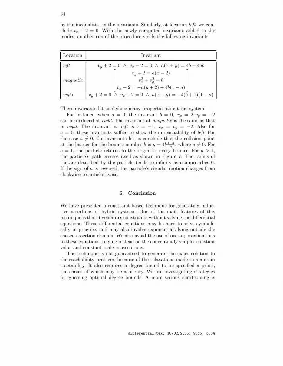
by the inequalities in the invariants. Similarly, at location left, we con-clude vx + 2 = 0. With the newly computed invariants added to themodes, another run of the procedure yields the following invariants

Location Invariant

left vy + 2 = 0 ∧ vx − 2 = 0 ∧ a(x+ y) = 4b− 4ab

magnetic

vy + 2 = a(x− 2)

v2x + v2

y = 8

vx − 2 = −a(y + 2) + 4b(1 − a)

right vy + 2 = 0 ∧ vx + 2 = 0 ∧ a(x− y) = −4(b+ 1)(1 − a)

These invariants let us deduce many properties about the system.For instance, when a = 0, the invariant b = 0, vx = 2, vy = −2

can be deduced at right. The invariant at magnetic is the same as thatin right. The invariant at left is b = −1, vx = vy = −2. Also fora = 0, these invariants suffice to show the unreachability of left. Forthe case a 6= 0, the invariants let us conclude that the collision pointat the barrier for the bounce number b is y = 4b1−a

a, where a 6= 0. For

a = 1, the particle returns to the origin for every bounce. For a > 1,the particle’s path crosses itself as shown in Figure 7. The radius ofthe arc described by the particle tends to infinity as a approaches 0.If the sign of a is reversed, the particle’s circular motion changes fromclockwise to anticlockwise.

6. Conclusion

We have presented a constraint-based technique for generating induc-tive assertions of hybrid systems. One of the main features of thistechnique is that it generates constraints without solving the differentialequations. These differential equations may be hard to solve symboli-cally in practice, and may also involve exponentials lying outside thechosen assertion domain. We also avoid the use of over-approximationsto these equations, relying instead on the conceptually simpler constantvalue and constant scale consecutions.

The technique is not guaranteed to generate the exact solution tothe reachability problem, because of the relaxations made to maintaintractability. It also requires a degree bound to be specified a priori,the choice of which may be arbitrary. We are investigating strategiesfor guessing optimal degree bounds. A more serious shortcoming is


35

that, at present, the technique does not handle inequalities. Inequalitiesfrequently occur in the guards and location conditions, and not beingable to use them in the constraint generation process may weaken theresulting invariants considerably. We are investigating strategies forextending the results in this paper to generate inequality invariants ofhybrid systems.

AcknowledgementWe would like to thank the anonymous referees for their careful readingof the paper and the many suggestions for improvement.

References

1. Asarin, E., Dang, T., and Maler, O. The d/dt tool for verification of hybridsystems. In Proc. 14th Intl. Conference on Computer Aided Verification (2002),vol. 2404 of LNCS, Springer Verlag, pp. 365–370.

2. Baader, F., and Nipkow, T. Term Rewriting and All That. CambridgeUniversity Press, 1998.

3. Bengtsson, J., Larsen, K. G., Larsson, F., Pettersson, P., and Yi,W. Uppaal — a Tool Suite for Automatic Verification of Real–Time Sys-tems. In Proc. of Workshop on Verification and Control of Hybrid Systems III(Oct. 1995), no. 1066 in Lecture Notes in Computer Science, Springer–Verlag,pp. 232–243.

4. Bensalem, S., Bozga, M., Fernandez, J.-C., Ghirvu, L., and Lakhnech,Y. A transformational approach for generating non-linear invariants. In StaticAnalysis Symposium (June 2000), vol. 1824 of LNCS, Springer Verlag.

5. Bockmayr, A., and Weispfenning, V. Solving numerical constraints. InHandbook of Automated Reasoning, A. Robinson and A. Voronkov, Eds., vol. I.Elsevier Science, 2001, ch. 12, pp. 751–842.

6. Collins, G. E., and Hong, H. Partial cylindrical algebraic decompositionfor quantifier elimination. Journal of Symbolic Computation 12, 3 (sep 1991),299–328.

7. Colon, M. Approximating the algebraic relational semantics of imperativeprograms. In 11th Static Analysis Symposium (SAS’2004) (2004), vol. 3148 ofLNCS, Springer-Verlag.

8. Colon, M., Sankaranarayanan, S., and Sipma, H. Linear invariant genera-tion using non-linear constraint solving. In Computer Aided Verification (July2003), F. Somenzi and W. H. Jr, Eds., vol. 2725 of LNCS, Springer Verlag,pp. 420–433.

9. Cousot, P., and Cousot, R. Abstract Interpretation: A unified lattice modelfor static analysis of programs by construction or approximation of fixpoints.In ACM Principles of Programming Languages (1977), pp. 238–252.

10. Cousot, P., and Halbwachs, N. Automatic discovery of linear restraintsamong the variables of a program. In ACM Principles of ProgrammingLanguages (Jan. 1978), pp. 84–97.

11. Cox, D., little, J., and O’Shea, D. Ideals, Varieties and Algorithms: AnIntroduction to Computational Algebraic Geometry and Commutative Algebra.Springer, 1991.


36

12. Forsman, K. Construction of Lyapunov functions using Grobner bases. InProc. 30th IEEE CDC (1991).

13. Garey, M., and Johnson, D. Computers and Intractability: A Guide to theTheory of NP-Completeness. W.H. Freeman & Co., New York, 1999.

14. Halbwachs, N., Proy, Y., and Roumanoff, P. Verification of real-timesystems using linear relation analysis. Formal Methods in System Design 11, 2(1997), 157–185.

15. Henzinger, T., and Ho, P.-H. Algorithmic analysis of nonlinear hybridsystems. In Computer-Aided Verification, vol. 939 of LNCS. Springer-Verlag,1995, pp. 225–238.

16. Henzinger, T. A. The theory of hybrid automata. In Logic In ComputerScience (LICS 1996) (1996), IEEE Computer Society Press, pp. 278–292.

17. Henzinger, T. A., and Ho, P. HyTech: The Cornell hybrid technology tool.In Hybrid Systems II (1995), vol. 999 of LNCS, Springer-Verlag, pp. 265–293.

18. Karr, M. Affine relationships among variables of a program. Acta Inf. 6(1976), 133–151.

19. Lafferriere, G., Pappas, G., and Yovine, S. Symbolic reachability compu-tation for families of linear vector fields. J. Symbolic Computation 32 (2001),231–253.

20. Manna, Z., and Pnueli, A. Temporal Verification of Reactive Systems:Safety. Springer-Verlag, New York, 1995.

21. Mishra, B., and Yap, C. Notes on Grobner bases. Information Sciences 48(1989), 219–252.

22. Muller-Olm, M., and Seidl, H. Polynomial constants are decidable. InStatic Analysis Symposium (SAS 2002) (2002), vol. 2477 of LNCS, Springer-Verlag, pp. 4–19.

23. Murata, T. Petri nets: Properties, analysis and applications. Proceedings ofthe IEEE 77, 4 (Apr. 1989), 541–580.

24. Parillo, P. A. Semidefinite programming relaxation for semialgebraicproblems. Mathematical Programming Ser. B 96, 2 (2003), 293–320.

25. Prajna, S., and Jadbabaie, A. Safety verification using barrier certificates.In Hybrid Systems: Computation and Control (2004), vol. 2993 of LNCS,Springer-Verlag, pp. 477–492.

26. Rodriguez-Carbonell, E., and Kapur, D. An abstract interpretationapproach for automatic generation of polynomial invariants. In 11th StaticAnalysis Symposium (SAS’2004) (2004), vol. 3148 of LNCS, Springer-Verlag.

27. Rodriguez-Carbonell, E., and Kapur, D. Automatic generation of poly-nomial loop invariants: Algebraic foundations. In Proc. Intl. Symp on Symbolicand Algebraic Computation (ISSAC-2004) (Spain, 2004).

28. Sankaranarayanan, S., Sipma, H., and Manna, Z. Non-linear loop in-variant generation using Grobner bases. In ACM Principles of ProgrammingLanguages (POPL) (2004), ACM Press, pp. 318–330.

29. Sankaranarayanan, S., Sipma, H. B., and Manna, Z. Petri net analy-sis using invariant generation. In Verification: Theory and Practice (2003),vol. 2772 of LNCS, Springer-Verlag, pp. 682–701.

30. Sankaranarayanan, S., Sipma, H. B., and Manna, Z. Constraint-basedlinear relations analysis. In 11th Static Analysis Symposium (SAS’2004) (2004),vol. 3148 of LNCS, Springer-Verlag, pp. 53–68.

31. Silva, B., Richeson, K., Krogh, B., and Chutinan, A. Modeling and veri-fying hybrid dynamic systems using CheckMate. In Proc. Conf. on Automationof Mixed Processes: Hybrid Dynamic Systems (2000), pp. 323–328.


37

32. Tiwari, A. Approximate reachability for linear systems. In Hybrid Systems:Computation and Control HSCC (2003), vol. 2623 of LNCS, Springer-Verlag,pp. 514–525.

33. Tiwari, A., and Khanna, G. Non-linear systems: Approximating reachsets. In Hybrid Systems: Computation and Control (2004), vol. 2993 of LNCS,Springer-Verlag, pp. 477–492.

34. Tiwari, A., Rueß, H., Saıdi, H., and Shankar, N. A technique for invari-ant generation. In TACAS 2001 (2001), vol. 2031 of LNCS, Springer-Verlag,pp. 113–127.

35. Windsteiger, W., and Buchberger, B. Grobner: A library for computingGrobner bases based on saclib. Tech. rep., RISC-Linz, 1993.

36. Yovine, S. Kronos: A verification tool for real-time systems. Springer In-ternational Journal of Software Tools for Technology Transfer 1, 1/2 (October1997).

Appendix

In this appendix, we shall prove a few useful theorems mentioned inother results along with the confluence of the Grobner basis reductionon templates. The key idea is to reduce any failure of confluence ontemplates to a failure of confluence on the instantiation of the templateunder an appropriate environment.

Claim 1. Let f, f ′ be templates and α be any environment.

1. α(f + g) = α(f) + α(g),

2. c · α(f) = α(c · f), for any c ∈ R.

Theorem 5 (Consistency). Let fp−→ f ′ for templates f, f ′, over

template variables in A. Then, for an arbitrary A-environment α, α(f)p−→

α(f ′) or α(f) = α(f ′). Conversely, if for some α, α(f)p−→ h then there

is a f ′ such that h = α(f ′) and fp−→ f ′.

Proof. We have that f ′ = f − c·tlt(p)p for some term c · t in f wherein

c(a0, . . . , am) is a linear expression. If α(c) = 0 then α(f) = α(f ′), or

else, if α(c) 6= 0 then we have that α(f ′) = α(f)− α(c·t)lt(p)p. In this case,

α(f)p−→ α(f ′).

On the other hand, let α(f)p−→ h, for some template f and poly-

nomial p. Let α(c) · t be the term in α(f) that lt(p) divides. Hence,the result of the reduction is,

h = α(f) − α(c)t

lt(p)p = α(f − ct

lt(p)p)

Therefore, setting f ′ = f− ctlt(p)p, we have α(f ′) = h and f

p−→ f ′.


38

Theorem 6 (Template Identity). Two templates f1, f2 over tem-plate variables A are not identical iff there is an environment α suchthat α(f1) 6≡ α(f2).

Proof. Since f1 6≡ f2, we have that f1 − f2 is a non-zero template. Lett be a term in f1 − f2, with a non-zero coefficient expression c. Let αbe an environment s.t. α(c) 6= 0. Hence α(f1 − f2) 6≡ 0. Thus we havethat α(f1) 6≡ α(f2).

The other direction is immediate from the definition of identicaltemplates.

Theorem 7 (Normal Form Theorem). A template f is a normal

form underG−→ iff for each environment α, α(f) is a normal form

underG−→.

Proof. To prove the forward implication, assume that f is a normal

form underG−→. However assume that α(f)

G−→ h for some α. By thereverse direction of the consistency theorem (Theorem 5), we have that

there exists f ′ such that fG−→ f ′ and α(f ′) = h. This contradicts our

assumption that f is in normal form.To prove the reverse implication, let us assume that f is not in

normal form. Then there is a reduction fG−→ f ′. Let t be the term in

f that is replaced by the reduction and c be its non-zero coefficient.By Theorem 5, we have that for each environment α, α(f) = α(f ′) or

α(f)G−→ α(f ′). We find an environment α such that α(c) 6= 0. For

such an environment α(f)G−→ α(f ′), since α(c) 6= 0. Thus α(f) is not

in normal form w.r.t.G−→.

Theorem 8 (Confluence of Templates). Let G be a Grobner basis

and f be a template. Let fG� f1 and f

G� f2, where f1, f2 are normal

forms. We have that f1 ≡ f2 and henceG−→ is confluent for templates.

Proof. Assuming otherwise, i.e., f1 6≡ f2, we have by Theorem 6 thatα(f1) 6≡ α(f2) for some α. Furthermore, Theorem 7 implies that α(f1)and α(f2) are in normal forms. By the forward direction of Theorem 5,

we have that α(f)G� α(fi), i = 1, 2. Hence, by the confluence of the

Grobner basis reduction relation over real polynomials, we have thatα(f1) = α(f2), thus leading to a contradiction.

Theorem 9 (Normal Forms for Templates). Let f be a templateover variables A. Let G be the Grobner basis of I = (G). Then, for anyA-environment α,

α(nfG(f)) = nfG(α(f))


39

Proof. The proof is by induction over the length of the minimal se-quence of reductions from f to f ′ = nf(f). For zero length derivations,f = nf(f), we have that α(f) is a normal form. Hence, α(nf(f)) =α(f) = nf(α(f)).

Assuming that the theorem holds for templates which have a length

n or less derivation to their normal forms, let fG−→ f1

G�n nf(f).

Hence, by Theorem 5, we have that α(f) = α(f1) or α(f)G−→ α(f1).

In either case nf(α(f1)) = nf(α(f)). Applying the induction to f1, wehave that α(nf(f1)) = nf(α(f1)). Hence

α(nf(f)) = α(nf(f1)) = nf(α(f1)) = nf(α(f))

Theorem 10 (Template Membership). Let f be a template andG be a Grobner basis, such that I = ((G)). Let f ′ = nfG(f). For eachenvironment α, α(f) ∈ I iff α(f ′) is identically zero.

Proof. Given f,G such that f ′ = nfG(f), for any environment α, wehave that α(f ′) = α(nf(f)) = nf(α(f)). Hence, if α(f ′) is identicallyzero, then nf(α(f)) is identically zero, and therefore, α(f) ∈ (G).

Let α(f) ∈ (G), hence nfG(α(f)) is identically zero. However, α(f ′) =α(nf(f)) = nf(α(f)) ≡ 0, and hence, α(nf(f)) = α(f ′) is identicallyzero.



Documents

Constructing invariants for hybrid systems