Embed Size (px)
Citation preview
1
Constructing Near-Perfect Phylogenies with Multiple Homoplasy
Events
Ravi Vijaya Satya, 1 Gabriela Alexe, 2 Laxmi Parida, 2Gyan Bhanot, 2 Amar Mukherjee 1
Abstract
In this paper, we explore the problem of constructing near-perfect phylogenies bi-allelic haplotypes,
where the deviation from perfect phylogeny is entirely due to recurrent mutations. We present some novel
insights into this problem and present polynomial-time algorithms for restricted versions of the problem.
We show that these algorithms can be extended to genotype data, in which case the problem is called the
near-perfect phylogeny haplotyping (NPPH) problem. Specifically, we present a near-optimal algorithm
for the H1-NPPH problem, which is to determine if a given set of genotypes admit a phylogeny with just
one homoplasy event. The time-complexity of our algorithm for the H1-NPPH problem is O(m2(n+m)),
where n is the number of genotypes and m is the number of SNP sites. This is a significant improvement
over the earlier algorithm with time-complexity O(n4).
We also introduce more generalized versions of the problem. The H(1, q)-NPPH problem is to deter-
mine if a given set of genotypes admit a phylogeny with q homoplasy events, so that all the homoplasy
events occur in a single site. Extending this definition even further, we define the H(p, q)-NPPH problem,
which is to determine if a given set of genotypes admit phylogeny in which at most p sites have homoplasy
events, with at most q homoplasy events in each site. We present an O(mq+1(n + m)) algorithm for the
H(1, q)-NPPH problem, and an O(nmp+1 + pmq+1(n + m)) algorithm for the H(p, q)-NPPH problem.
Keywords: Haplotype Inference, Perfect Phylogeny, Near-perfect phylogeny haplotyping
1 Introduction
Though the genomic sequence is mostly similar from individual to individual, each individual differs from others in
some locations. Studying these variations will help in understanding, diagnosis, and treatment of many genetically
inherited diseases. Single Nucleotide Polymorphisms (SNPs) are the most common genetic variations observed. SNPs
are loci in the human genome where multiple variants exist at a high enough frequency (> 0.05) that the position
can be considered polymorphic within the population. Each individual variant in a SNP location is called an allele.
It is estimated [HapMapConsortium, 2003] that there are as many as 10 million SNPs in the human genome, which
translates to a density of one SNP every three hundred base pairs of DNA. More than 99% of the SNPs in the human
genome are bi-allelic.
The human genome is diploid, meaning that in each cell there are two copies of each chromosome. Due to the
bi-parental nature of heredity in diploid organisms, one of these copies is derived from the mother and the other is
derived from the father. Each of these copies is called a haplotype. As we are interested in only the SNP locations, in
1University of Central Florida, Orlando FL 32816, USA.2IBM T.J. Watson Research Center, York Town Heights NY 10549, USA
Email: [email protected], [email protected], [email protected], [email protected], [email protected]
the genome, a haplotype that covers a region of the chromosome with m SNPs is generally represented as a binary
vector of length m. The values 0 and 1 represent the two alleles of each SNP. A genotype gives combined information
about the two haplotypes, and is represented by length-m vector over the alphabet {0, 1, 2}. In a genotype g, if g[i] is
0 or 1, it implies that the two haplotypes (h, h′) for g are homozygous in the ith SNP with the 0-allele or the 1-allele,
respectively. If g[i] = 2, it implies that the ith SNP is heterozygous in g. i.e., either h[i] = 0 and h′[i] = 1, or h[i] = 1
and h′[i] = 0.
With the current technology, the cost associated with empirically collecting haplotype data is prohibitively expen-
sive. Therefore, only the un-ordered bi-allelic genotype data is collected through empirical means. This necessitates
computational techniques for inferring the most haplotypes from the genotypes. Given n genotypes over m SNP sites,
the haplotype inference(HI) is to find a pair of haplotypes for each genotype, so that combining the two haplotypes
results in the genotype. This problem is also referred to as the phase problem in genotyping. For each genotype, we
want to find the most likely pair of haplotypes that might have combined to form the genotype.
The haplotype inference problem was first introduced by Clark [Clark, 1990]. Subsequently, multiple formulations
were introduced, with different definitions for the optimum solution. Most formulations are based on parsimony,
perfect phylogeny or maximum likelihood. A comprehensive survey of the many different variations of the HI problem
is provided by [Bonizzoni et al., 2003].
1.1 Perfect Phylogeny
Under the coalescent model of evolution, all the individuals in a population have a common ancestor. Applying the
standard infinite sites assumption to the coalescent model leads to the perfect phylogeny model of evolution, which
assumes that each site in the genome can mutate only once in the evolutionary history. A perfect phylogeny T for n
haplotypes over m SNPs is a tree in which each of the m SNPs labels exactly one edge in the T . Each vertex in T is
labeled by a haplotype vector. Each of the n haplotypes must label some vertex in the tree.
Applying the coalescent model to the Haplotype Inference problem, Gusfield [Gusfield, 2002] introduced a perfect
phylogeny formulation of the problem, called the PPH(Perfect Phylogeny Haplotyping) problem. The perfect phy-
logeny formulation requires that all the haplotypes that resolve the given genotypes describe a perfect phylogeny. The
perfect phylogeny model is justified by the block structure of the human genome and the validity of the infinite sites
assumption. The block structure guarantees that there are few (ideally zero) recombinations within the block, and
the infinite-sites assumptions guarantees that each site mutates only once in the recent evolutionary history under
consideration.
Gusfield [Gusfield, 2002] presented an O(nm2) algorithm for the PPH problem by reduction to the graph re-
alization problem. The paper also lays out some fundamental rules that help in determining if a solution exists,
and finding the solution if there is one. Bafna et al [Bafna et al., 2002] presented a direct solution that takes
O(nmα(nm)) time. Eskin et al [Eskin et al., 2003] presented an alternative approach to the problem, but the
overall complexity is still O(nm2). The authors of this paper have have recently developed the optimal O(nm)
OPPH algorithm [VijayaSatya and Mukherjee, 2005a, VijayaSatya and Mukherjee, 2006]. A new data structure
called the FlexTree which represents all the phylogenetic trees for a given PPH problem was presented in in
[VijayaSatya and Mukherjee, 2005a, VijayaSatya and Mukherjee, 2006]. The OPPH algorithm makes use of this
FlexTree data structure in order to solve the PPH problem in the optimal O(nm) time. Two other simultane-
2
ous, independent O(nm) algorithms [Liu and Zhang, 2004, Ding et al., 2005] have also been developed for the PPH
problem.
1.2 Imperfect Phylogeny
True biological data rarely, if ever, conforms to perfect phylogeny because of repeated mutations and recombinations.
However, the deviations from perfect phylogeny are expected to be small within a block of the human genome. When
the deviations from perfect phylogeny are small, and the phylogenies are called as near-perfect phylogenies. The
term near perfect phylogeny is generally used to refer to phylogenies that involve a small number of repeated/back
mutations.
The problem of constructing near perfect phylogenies with repeated mutations has been tackled before [Fernandez-Baca and Lagergren,
The complexity of the best algorithm for constructing near perfect phylogenies on a set of n haploid taxa is given by
nmO(q)2O(q2r2), where r is number of alleles in any site, and q is the repeated/back mutations. In this paper, we are
only concerned with bi-allelic SNP data, and hence r = 2. Even then the algorithm is clearly impractical for values
of q as small as 4.
In this paper, we deal with restricted versions of the near-perfect phylogeny problem and present polynomial
time algorithms for these problems. Song et al.[Song et al., 2005] have introduced a restricted version of the near-
perfect phylogeny problem that allows a single repeated mutation. They specifically defined the problem on genotype
data and called the problem the H1 Imperfect Phylogeny Haplotyping (H1-IPPH) problem. However, the acronym
IPPH has been previously used [Halperin and Karp, 2004, Kimmel and Shamir, 2005] to refer to the Incomplete
Perfect Phylogeny Haplotyping problem. Therefore, in this paper, we rename the problem as the H1- Near-Perfect
Phylogeny Haplotyping problem (H1-NPPH).
In this paper, we present a generalized framework for constructing near-perfect phylogenies(NPPs) that involve
more than one homoplasy events, both for haplotype and genotype data. We define a H(1, q) NPP as a near-perfect
phylogeny involving q homoplasy events in a single site. Similarly, a H(p, q)-NPP is a near perfect phylogeny, in which
p sites have homoplasy events, with at most q homoplasy events in each site. Under this notation, a near-perfect
phylogeny with a single homoplasy is denoted as the H(1, 1)-NPP.
In Section 2, we present polynomial-time algorithms for constructing near-perfect phylogenies for haplotype
data. In Section ??, we extend these algorithms to deal with genotype data. The algorithms we present here are
near-optimal for the problems involved. Specifically, our O(m2(n + m) algorithm for the H1-NPPH problem is a
significant improvement over the earlier O(n4) algorithm presented in [Song et al., 2005]. We have implemented the
H1-NPPH algorithm using C++. Testing on simulated data, we show that our algorithm is very fast while having
comparable accuracy to that of the popular PHASE [Stephens et al., 2001] program. The speed of the H1-NPPH
implementation proves that the this approach is practical H(p, q)-NPPH problem, specifically for small values of p
and q. **********re-phrase the previous sentence********.
2 Constructing Near-Perfect Phylogenies from Haplotype data
In this section, we present polynomial-time algorithms for various restricted versions of Near-Perfect Phylogeny (NPP)
problem. In all the problems that we describe in this section, the input is an n×m matrix M over the alphabet {0, 1},
3
c4
c1
c2
c3
c5
c1
11000
01000
00100
00011
10010
00010
00000
11000
01001
00100
00010
00011
5
4
3
2
1
54321
r
r
r
r
r
ccccc
(a) (b)
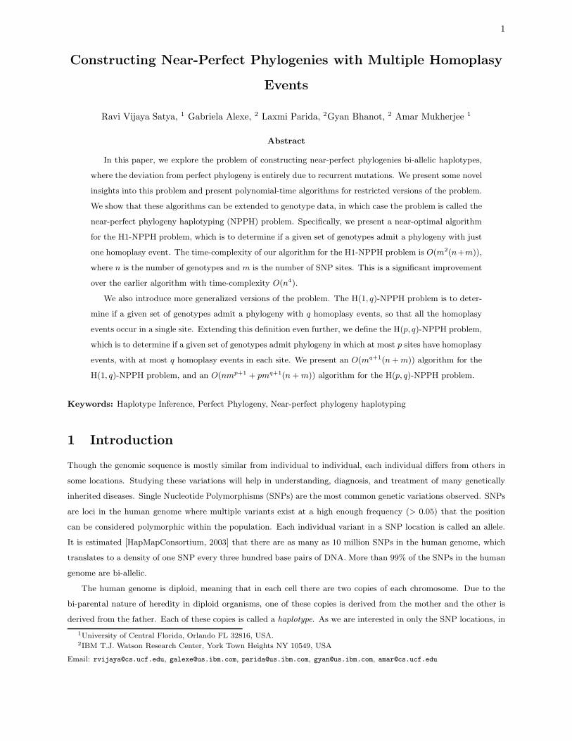
Figure 1: (a) A haplotype matrix M ; (b) A phylogeny T for M
where the columns c1, c2, ..., cm indicate sites and the rows r1, r2, ..., rn indicate samples. Given that the matrix M
does not allow a perfect phylogeny, we want to construct a near-perfect phylogeny for M that is the closest to a
perfect phylogeny. We use the terms ‘column’ and ‘site’ interchangeably in the rest of this paper.
Throughout this paper we assume that the deviations from perfect phylogeny are only due to violations of the
infinite sites assumption - i.e, due to recurrent or back mutations. The phylogenies we deal with in this paper are
un-rooted phylogenies. In an un-rooted phylogeny, there is no distinction between a recurrent mutation and a back
mutation.
We define the following terms. An ordered pair of values (a, b), aǫ{0, 1}, bǫ{0, 1}, is said to be induced by a
pair of ordered columns (i, j) if there is a row r in M such that M [r, i] = a and M [r, j] = b. The set of ordered
pairs induced by a pair of columns (i, j) is denoted by I(i, j). According to the well-established four-gamete test
[Hudson and Kaplan, 1985], the matrix M does not have a perfect phylogeny if |I(i, j)| = 4 for any pair of columns
(i, j). We say that two columns i and j conflict with each other if |I(i, j)| = 4. A conflict graph Gc = (V, E) is a
graph in which each vertex viǫV corresponds to a column ci in M . An edge (vi, vj) is in E if the sites ci and cj
conflict with each other.
The general definition of a phylogeny is that the phylogeny is a tree in which the leaves represent the input taxa.
In this paper, we are more interested in the structure of the phylogeny than the actual phylogeny of the taxa. Hence,
when we say a phylogeny, we refer to an edge and vertex labeled tree T . Each edge in T is labeled by a site in M ,
and indicates a mutation in that site. An example of a phylogeny is shown in Figure 1. Each vertex in the phylogeny
is labeled by 0-1 vector of length m, and indicates the state of each site at the vertex. For any vertex v, we denote
the vertex label of v using the notation L(v). Since T is a phylogeny for M , for each row r in M , there must be a
vertex v such that L(v) = M [r]. Multiple rows in M might map to the same vertex in T , and some vertices in T
might not represent any row in M . Notice that the phylogeny in Figure 1 is not a perfect phylogeny. There are two
edges in T labeled with column c1.
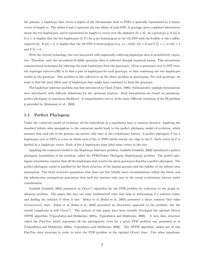
Removing a set of vertices Sc from any tree T divides T into a set of connected (trivial or non-trivial) components
denoted as T/Sc. Note that, since T is a tree, each connected component TiǫT/Sc
will also be a tree. For any connected
component Ti of T , we define R(Ti) as the set of rows of M that map to any vertex in Ti. A column c is said to be
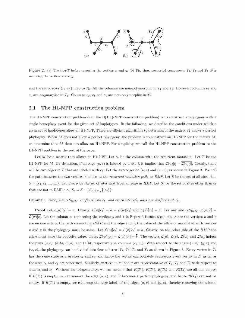
non-polymorphic in Ti if the column c has the same state in each row rǫR(Ti). For example, refer to Figure 2-(a),
which is the same phylogeny as in Figure 1. The three connected components produced by removing the vertices x
and y in 2-(a) are shown in Figure 2-(b)[in dotted regions]. In the matrix M , the row r2 maps to T1, r3 maps to T2,
4
(b)
c4
c1
c2
c3
c5
c1
x
y c5
c1
y
x
T1
T2
T3
(a)
Figure 2: (a) The tree T before removing the vertices x and y; (b) The three connected components T1, T2 and T3 after
removing the vertices x and y
and the set of rows {r4, r5} map to T3. All the columns are non-polymorphic in T1 and T2. However, columns c5 and
c1 are polymorphic in T3. Columns c2, c3 and c4 are non-polymorphic in T3.
2.1 The H1-NPP construction problem
The H1-NPP construction problem (i.e., the H(1, 1)-NPP construction problem) is to construct a phylogeny with a
single homoplasy event for the given set of haplotypes. In the following, we describe the conditions under which a
given set of haplotypes allow an H1-NPP. There are efficient algorithms to determine if the matrix M allows a perfect
phylogeny. When M does not allow a perfect phylogeny, the problem is to construct an H1-NPP for the matrix M ,
or determine that M does not allow an H1-NPP. For simplicity, we call the H1-NPP construction problem as the
H1-NPP problem in the rest of the paper.
Let M be a matrix that allows an H1-NPP. Let cb be the column with the recurrent mutation. Let T be the
H1-NPP for M . By definition, if an edge (u, v) is labeled by a site i, it implies that L(u)[i] = L(v)[i]. Clearly, there
will be two edges in T that are labeled with cb. Let the two edges be (u, v) and (w, x), as shown in Figure 3. We call
the path between the two vertices v and w as the recurrent mutation path, or RMP. Let S be the set of all sites, i.e.,
S = {c1, c2, ..., cm}. Let SRMP be the set of sites that label an edge in RMP. Let Se be the set of sites other than cb
that are not in RMP. i.e., Se = S − {SRMP
⋃{cb}}.
Lemma 1 Every site cǫSRMP conflicts with cb, and every site cǫSe does not conflict with cb.
Proof Let L(u)[cb] = a. Clearly, L(v)[cb] = a = L(w)[cb] and L(x)[cb] = a. For any site cǫSRMP , L(v)[c] =
L(w)[c]. Let the column c1 connecting the vertices y and z in Figure 3 is such a column. Since the vertices u and v
are on one side of the path connecting RMP and the edge (u, v), the value of the allele c1 associated with vertices
u and v in the phylogeny must be same. Let L(u)[c1] = L(v)[c1] = b. Clearly, on the other side of the RMP the
allele must have the opposite value. Thus, L(w)[c1] = L(x)[c1] = b. The vectors L(u), L(v), L(w) and L(x) induce
the pairs (a, b), (a, b), (a, b), and (a, b), respectively in columns (cb, c1). With respect to the edges (u, v), (y, z) and
(w, x), the phylogeny can be divided into four subtrees T1, T2, T3 and T4 as shown in Figure 3. Every vertex in T1
has the same state as u in sites cb and c1, and hence the vertex appropriately represents every vertex in T1 as far as
the sites cb and c1 are concerned. Similarly, vertices v, w, and x are representative of T2, T3 and T4 with respect to
sites c1 and cb. Without loss of generality, we can assume that R(T1), R(T2), R(T3) and R(T4) are all non-empty.
If R(T1) is empty, we can remove the edge (u, v), and T becomes a perfect phylogeny, and hence R(T1) can not be
empty. If R(T2) is empty, we can swap the edge-labels of the edges (u, v) and (y, z), thereby removing the column
5
cb cb
T1
u v w x
c3
c1 y z
T2
T4
T3 c4 c2
Figure 3: Illustration of Lemma 1
c1 from RMP. Hence, R(T2) cannot be empty. R(T3) cannot be empty for the same reasons as that of R(T2), and
R(T4) cannot be empty for the same reasons as that of R(T1). Hence, the pairs (a, b), (a, b), (a, b), and (a, b) will all
be in I(cb, c1). Therefore, |I(cb, c1)| = 4, and hence cb conflicts with c1.
It can similarly be shown that every site cǫSe will not conflict with cb. Sites c2, c3 and c4 in Figure 3 are examples
of such sites. ♦
Let T/{u,v,w,x} be the set of connected components generated by removing vertices u, v, w and x from T . Removing
the vertices u, v, w and x removes both the edges labeled with cb from T . Therefore, no connected component in
T/{u,v,w,x} will have an edge labeled with cb. Therefore, the column cb will be non-polymorphic within any connected
component TiǫT/{u,v,w,x}.
We will now state and prove a theorem that gives the necessary and sufficient conditions for a haplotype matrix
to have a perfect phylogeny with only one homoplasy event. Let M be a matrix such that M does not allow a perfect
phylogeny, but the matrix M ′ produced by removing a column cb from M allows a perfect phylogeny T ′. Since the
rows in M correspond one-to-one with rows in M ′, the rows in M can be mapped to vertices in T ′. It will be helpful
to visualize the matrix M as the matrix M ′ with a single column cb appended as the rightmost column of M . We
state the following theorem:
Theorem 1 The matrix M allows an H1-NPP iff there are two vertices x and y in T ′ such that the site cb is
non-polymorphic in every connected component in T ′/{x,y}.
Proof Let T ′/{x,y} = {T1, T2, ....Tk}, as shown in Figure 4-(a), where k = d(x) + d(y) − 1, d(x) is the degree of x
and d(y) is the degree of y in T ′. We show that we can construct an H1-NPP T for M by expanding the vertices
x and y into edges labeled with cb. We start with an empty tree T . We introduce four new vertices x0, x1, y0 and
y1 into T , and add two edges (x0, x1) and (y0, y1), both labeled with cb. The two vertices x0 and x1 are labeled
based on the label of the vertex x in T ′ as follows - L(x0)[i] = L(x1)[i] = L(x)[i] for every column i 6= cb. This is
equivalent to taking the matrix M ′ and attaching the vertex label of x in T ′ to both the vertices x0 and x1. This
takes care of the allele values of all sites except the site cb. The site cb is now associated with the edge (x0, x1) as
follows: L(x0)[cb] = 0, and L(x1)[cb] = 1. The vertices y0 and y1 are similarly labeled based the label of the vertex in
y in T ′ in every site other than cb. In site cb, L(y0)[cb] = 0 and L(y1)[cb] = 1. With reference to Figure 4-(b),in each
component Ti, 1 ≤ i ≤ j, there will be a vertex vi so that (x, vi) is an edge in T ′. Since Ti is non-polymorphic in cb,
we can introduce the edge (x0, vi) or (x1, vi) in T , depending on whether L(v)[cb] = 0, or L(v)[cb] = 1, respectively.
Similarly, each component from Tj+2 to Tk can be connected to either y0 or y1, as shown in Figure 4-(b). If Tj+1 is
non-empty, there will be vertices v1 and v2 in Tj+1 so that (x, v1) and (y, v2) are edges in T ′. If L(v1)[cb] = 0, we
6
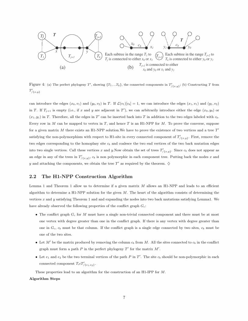
x y
Tj
T1 Tj+1
Tj+2
Tk
x0 x1 y1 y0
cb cb
Tj+1
Tj+1 is connected to either
x0 and y0 or x1 and y1
T�
T
Each subtree in the range T1 to
Tj is connected to either x0 or x1
Each subtree in the range Tj+2 to
Tk is connected to either y0 or y1
(a) (b)
Figure 4: (a) The perfect phylogeny T ′, showing {T1, ...Tk}, the connected components in T ′/{x,y}
; (b) Constructing T from
T ′/{x,y}
can introduce the edges (x0, v1) and (y0, v2) in T . If L(v1)[cb] = 1, we can introduce the edges (x1, v1) and (y1, v2)
in T . If Tj+1 is empty (i.e., if x and y are adjacent in T ′), we can arbitrarily introduce either the edge (x0, y0) or
(x1, y1) in T . Therefore, all the edges in T ′ can be inserted back into T in addition to the two edges labeled with cb.
Every row in M can be mapped to vertex in T , and hence T is an H1-NPP for M . To prove the converse, suppose
for a given matrix M there exists an H1-NPP solution.We have to prove the existence of two vertices and a tree T ′
satisfying the non-polymorphism with respect to H1-site in every connected component of T ′/{x,y}. First, remove the
two edges corresponding to the homoplasy site cb and coalesce the two end vertices of the two back mutation edges
into two single vertices. Call these vertices x and y.Now obtain the set of trees T ′/{x,y}. Since cb does not appear as
an edge in any of the trees in T ′/{x,y}, cb is non polymorphic in each component tree. Putting back the nodes x and
y and attaching the components, we obtain the tree T ′ as required by the theorem. ♦
2.2 The H1-NPP Construction Algorithm
Lemma 1 and Theorem 1 allow us to determine if a given matrix M allows an H1-NPP and leads to an efficient
algorithm to determine a H1-NPP solution for the given M . The heart of the algorithm consists of determining the
vertices x and y satisfying Theorem 1 and and expanding the nodes into two back mutations satisfying Lemma1. We
have already observed the following properties of the conflict graph Gc:
• The conflict graph Gc for M must have a single non-trivial connected component and there must be at most
one vertex with degree greater than one in the conflict graph. If there is any vertex with degree greater than
one in Gc, cb must be that column. If the conflict graph is a single edge connected by two sites, cb must be
one of the two sites.
• Let M ′ be the matrix produced by removing the column cb from M . All the sites connected to cb in the conflict
graph must form a path P in the perfect phylogeny T ′ for the matrix M ′.
• Let e1 and e2 be the two terminal vertices of the path P in T ′. The site cb should be non-polymorphic in each
connected component TiǫT′/{e1,e2}
.
These properties lead to an algorithm for the construction of an H1-IPP for M .
Algorithm Steps
7
c3 c7
c5 c1
c2
c4 c6
c8 c9
(c)
(d)
c6
c7
c5
c4
c2
c1 c9 c8
r1
r2 r3
r4
r5
r6 r9
r8 r10
x0 y0 r7
c3 y1
c3
x1
101100100
001100100
011100000
001100000
000110110
000110101
000111000
000110000
000100000
000000000
10
9
8
7
6
5
4
3
2
1
987654321
r
r
r
r
r
r
r
r
r
r
ccccccccc
M Gc (b)
(a)
x c2 y
r1 r4
r5
r6
r10
r7,r9
c9 c4 c1
r8
c6 c8
c5 c7 r2 r3
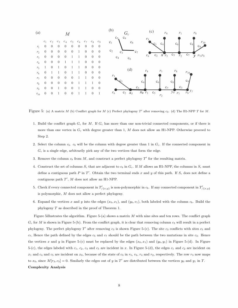
Figure 5: (a) A matrix M (b) Conflict graph for M (c) Perfect phylogeny T ′ after removing c3. (d) The H1-NPP T for M .
1. Build the conflict graph Gc for M . If Gc has more than one non-trivial connected components, or if there is
more than one vertex in Gc with degree greater than 1, M does not allow an H1-NPP. Otherwise proceed to
Step 2.
2. Select the column cb. cb will be the column with degree greater than 1 in Gc. If the connected component in
Gc is a single edge, arbitrarily pick any of the two vertices that form the edge.
3. Remove the column cb from M , and construct a perfect phylogeny T ′ for the resulting matrix.
4. Construct the set of columns Sc that are adjacent to cb in Gc. If M allows an H1-NPP, the columns in Sc must
define a contiguous path P in T ′. Obtain the two terminal ends x and y of this path. If Sc does not define a
contiguous path T ′, M does not allow an H1-NPP.
5. Check if every connected component in T ′/{x,y} is non-polymorphic in cb. If any connected component in T ′
/{x,y}
is polymorphic, M does not allow a perfect phylogeny.
6. Expand the vertices x and y into the edges (x0, x1), and (y0, v1), both labeled with the column cb. Build the
phylogeny T as described in the proof of Theorem 1.
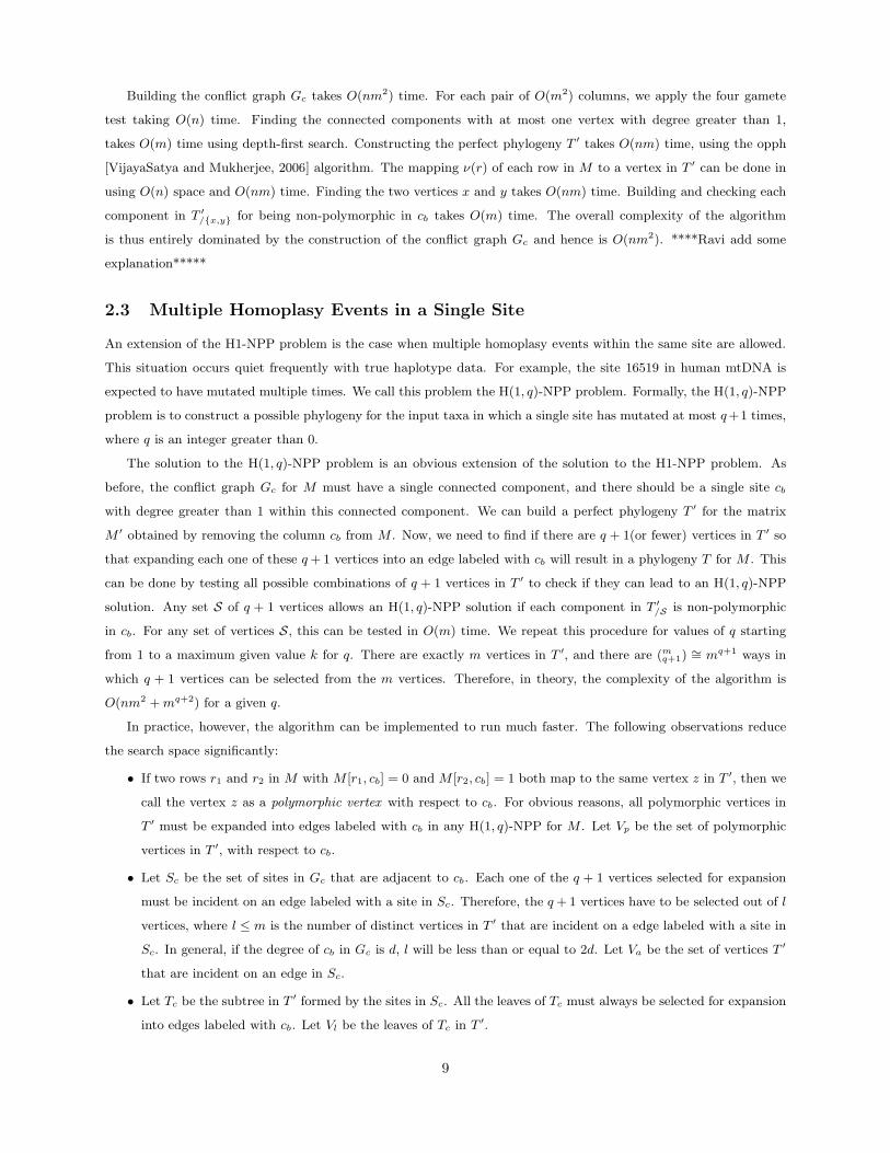
Figure 5illustrates the algorithm. Figure 5-(a) shows a matrix M with nine sites and ten rows. The conflict graph
Gc for M is shown in Figure 5-(b). From the conflict graph, it is clear that removing column c3 will result in a perfect
phylogeny. The perfect phylogeny T ′ after removing c3 is shown Figure 5-(c). The site c3 conflicts with sites c5 and
c7, Hence the path defined by the edges c5 and c7 should be the path between the two mutations in site c3. Hence
the vertices x and y in Figure 5-(c) must be replaced by the edges (x0, x1) and (y0, y1) in Figure 5-(d). In Figure
5-(c), the edges labeled with c1, c2, c4 and c5 are incident in x. In Figure 5-(d), the edges c1 and c2 are incident on
x1 and c4 and c5 are incident on x0, because of the state of c3 in r5, r6, r4 and r2, respectively. The row r3 now maps
to x0, since M [r3, c3] = 0. Similarly the edges out of y in T ′ are distributed between the vertices y0 and y1 in T .
Complexity Analysis
8
Building the conflict graph Gc takes O(nm2) time. For each pair of O(m2) columns, we apply the four gamete
test taking O(n) time. Finding the connected components with at most one vertex with degree greater than 1,
takes O(m) time using depth-first search. Constructing the perfect phylogeny T ′ takes O(nm) time, using the opph
[VijayaSatya and Mukherjee, 2006] algorithm. The mapping ν(r) of each row in M to a vertex in T ′ can be done in
using O(n) space and O(nm) time. Finding the two vertices x and y takes O(nm) time. Building and checking each
component in T ′/{x,y} for being non-polymorphic in cb takes O(m) time. The overall complexity of the algorithm
is thus entirely dominated by the construction of the conflict graph Gc and hence is O(nm2). ****Ravi add some
explanation*****
2.3 Multiple Homoplasy Events in a Single Site
An extension of the H1-NPP problem is the case when multiple homoplasy events within the same site are allowed.
This situation occurs quiet frequently with true haplotype data. For example, the site 16519 in human mtDNA is
expected to have mutated multiple times. We call this problem the H(1, q)-NPP problem. Formally, the H(1, q)-NPP
problem is to construct a possible phylogeny for the input taxa in which a single site has mutated at most q+1 times,
where q is an integer greater than 0.
The solution to the H(1, q)-NPP problem is an obvious extension of the solution to the H1-NPP problem. As
before, the conflict graph Gc for M must have a single connected component, and there should be a single site cb
with degree greater than 1 within this connected component. We can build a perfect phylogeny T ′ for the matrix
M ′ obtained by removing the column cb from M . Now, we need to find if there are q + 1(or fewer) vertices in T ′ so
that expanding each one of these q + 1 vertices into an edge labeled with cb will result in a phylogeny T for M . This
can be done by testing all possible combinations of q + 1 vertices in T ′ to check if they can lead to an H(1, q)-NPP
solution. Any set S of q + 1 vertices allows an H(1, q)-NPP solution if each component in T ′/S is non-polymorphic
in cb. For any set of vertices S , this can be tested in O(m) time. We repeat this procedure for values of q starting
from 1 to a maximum given value k for q. There are exactly m vertices in T ′, and there are (mq+1) ∼= mq+1 ways in
which q + 1 vertices can be selected from the m vertices. Therefore, in theory, the complexity of the algorithm is
O(nm2 + mq+2) for a given q.
In practice, however, the algorithm can be implemented to run much faster. The following observations reduce
the search space significantly:
• If two rows r1 and r2 in M with M [r1, cb] = 0 and M [r2, cb] = 1 both map to the same vertex z in T ′, then we
call the vertex z as a polymorphic vertex with respect to cb. For obvious reasons, all polymorphic vertices in
T ′ must be expanded into edges labeled with cb in any H(1, q)-NPP for M . Let Vp be the set of polymorphic
vertices in T ′, with respect to cb.
• Let Sc be the set of sites in Gc that are adjacent to cb. Each one of the q + 1 vertices selected for expansion
must be incident on an edge labeled with a site in Sc. Therefore, the q + 1 vertices have to be selected out of l
vertices, where l ≤ m is the number of distinct vertices in T ′ that are incident on a edge labeled with a site in
Sc. In general, if the degree of cb in Gc is d, l will be less than or equal to 2d. Let Va be the set of vertices T ′
that are incident on an edge in Sc.
• Let Tc be the subtree in T ′ formed by the sites in Sc. All the leaves of Tc must always be selected for expansion
into edges labeled with cb. Let Vl be the leaves of Tc in T ′.
9
Let mc = |Va|, and let mg = |Vp
⋃Vl|. The actual number of sets that need to be searched is given by (
mc−mg
q+1−mg).
Hence, for any matrix M , q must be greater than or equal to mg − 1.
2.4 Allowing Homoplasy Events in Multiple Sites
Extending the problem even further, we define the H(p, q)-NPP problem. An H(p, q)-NPP is a phylogeny in which
at most p sites have homoplasy events, with at most q homoplasy events in each site. The conflict graph in this case
will have multiple connected components and/or multiple vertices with degree greater than 1.
Let G′c be the graph obtained by removing all degree-0 vertices from Gc. If the matrix M is to allow an H(p, q)-
NPP, G′c must have a vertex cover with size less than or equal to p. If such a vertex cover C is found, removing the
vertices in C from Gc will result in a graph with no non-trivial connected components. We will be able to construct
a perfect phylogeny T ′ for the vertices in SC. Once T ′ is constructed, we can add the sites in C to T ′ one by one.
The order in which the sites are added to T ′ does not matter. Adding each site to T ′ is essentially an H(1, q)-NPP
problem.
The problem of finding the minimum vertex cover is NP-complete. Therefore, finding all vertex covers in G′c with
size at most p takes exponential time with respect to p. Though the possibility of G′c having multiple connected
components somewhat breaks down the problem into smaller parts, effectively the solution is to try all possible sets
of vertices in G′c with size p to check if they form a vertex cover for G′
c. Assuming the size of Gc is O(m), finding all
such vertex covers takes O(mp+1) time. For each vertex cover, we need to construct the initial perfect phylogeny T ′,
and keep adding sites from C to T ′. As explained above, this is equivalent to solving p H(1, q)-NPP problems. Hence
the over all complexity of the problem is O(nm2 + mp+1 + ηpmq+2) time, where η is the number of distinct vertex
covers of G′c with size less than or equal to p.
Special Scenarios
A special situation arises when each non-trivial connected component in Gc has at most one site with degree greater
than 1. In that case, p will be equal to the number of non-trivial connected components in Gc. The set C (described
above) is fixed. This reduces the time complexity of the algorithm to O(nm2 + pmq+2). In general, each connected
component in Gc that is either a single edge or involves a single vertex with degree greater than 1 will reduce the
effective value of p by 1.
3 Near-Perfect Phylogeny Haplotyping
In case of the NPPH problem, the input is a set of genotypes. The aim in general is to construct a set of haplotypes
that are the most likely explanation for the given set of genotypes. Parsimony is widely accepted as the most likely
explanation. Therefore, the aim is to obtain, out of all possible explanations for the given genotypes, the set of
haplotypes that a allows a phylogeny with the least number of recurrent mutations. The unrestricted version of this
problem is clearly NP-complete. Here, we try to solve some restricted versions of the problem.
3.1 H1-NPPH Problem
We formally state the H1-NPPH problem as follows. We are given an n × m genotype matrix A over the alphabet
{0, 1, 2}. Each row in A represents a genotype. As before, the columns represent SNP sites. The aim is to construct
10
a 2n × m haplotype matrix M such that 1) Each row r in A is a result of combining the rows r and r′ in M and 2)
The matrix M allows an H1-NPP.
The solution to the H1-NPPH problem is very similar to that for the H1-NPP problem, except that it might not
be possible to fully construct the conflict graph for a genotype matrix. In a genotype matrix A, an ordered pair of
values (a, b), aǫ{0, 1}, bǫ{0, 1} is in I(i, j) for a pair of columns (i, j) if
1. There is a row r in A such that A[r, i] = a and A[r, j] = b,or
2. A[r, i] = a and A[r, j] = 2, or
3. A[r, i] = 2 and A[r, j] = b.
If two columns i and j are ‘2’ in some genotype, the states of i and j in the two haplotypes for the genotype could
be either {(0, 0), (1, 1)} or {(0, 1), (1, 0)}. Therefore, we might not be able to completely specify I(i, j). I(i, j) can be
completely specified only in two situations: when I(i, j) = 4 because of rows in A in which either the column i or the
column j is not ‘2’ or when there are no rows in A in which both i and j are ‘2’. Hence, though we might be able to
construct some edges in the conflict graph in Gc, we might not be able to construct all the edges in Gc.
Since we can not construct Gc directly, we need other ways to find the column cb that has a recurrent mutation.
One obvious procedure for finding cb is to remove each column from A, and check if the rest of the matrix allows
a perfect phylogeny. If we can find such a column cb, then there might be a H1-NPPH solution for A. This is the
procedure used in [Song et al., 2005] to find the column cb. We adopt the same procedure to find cb. Then, we
propose our new algorithm to construct H1-NPPH.
Once the column cb is found, we can build the perfect phylogeny T ′ for the matrix A′ obtained by removing cb from
A. In general, the matrix A′ might have multiple perfect phylogenies. Chung and Gusfield [Chung and Gusfield, 2002]
have empirically shown that the likelihood for the phylogeny being unique increases quickly with the number of
genotypes. Even for relatively small data sets of 50 individuals and 50 SNP sites, it has been shown that the PPH
solution is unique 99.9% of the time. In the following, we assume that A′ has a unique perfect phylogeny T ′. If A′
allows multiple perfect phylogenies, the following procedure has to be repeated for each such perfect phylogeny.
Using the phylogeny T ′, we can construct the haplotype matrix M ′ for A′. We denote the rows of A′ by r1, r2, ...
and the corresponding pairs rows in M ′ as r1, r′1, r2, r
′2, ... The matrix M should now be built by adding the column
cb to M ′. We can also assign values to some rows in column cb of the matrix M . In a row ri of A′, if A′[ri, cb]
is either 0 or 1, then both the haplotypes for this row will also have either 0 or 1, respectively. We then set
M [ri, cb] = M [r′i, cb] = A′[ri, cb]. When A′[r, cb] = 2, we know that M [ri, cb] = M [r′i, cb], but we can not determine
which one of them must be 0 for M to allow an H1-NPP. We call such a pair of rows (ri, r′i) in M as an ambiguous
pair. Thus the problem of determining whether A allows an H1-NPP solution reduces to determining whether there
is an assignment of values to each such ambiguous pair so that matrix M allows an H1-NPP.
Each row in M ′ (and hence in M) can be mapped to a vertex in T ′. We represent this mapping using the notation
ν(ri) = v, where ri is a row in M , and v is a vertex in T ′. For any vertex v in T ′, zero or more rows in M can map
to vertex v.
The underlying idea of our algorithm is based on Theorem 1 which was used to find a path RMP defined by two
end points of the recurrent mutations. For this we need to identify two vertices x and y, if they exist, such that each
connected component in T ′/{x,y} is polymorphic with respect to cb. We will show how to use this property to actually
obtain an assignment of values to each ambiguous pair of rows in M .
11
We choose arbitrarily two vertices x and y in T ′ and construct a graph Ga = (V, E), where the vertices in V
correspond to a connected component TiǫT′/{x,y}. For each ambiguous pair (ri, r
′i) in M , we know that M [ri, cb] =
M [r′i, cb]. Therefore, if ν(ri) is in a component Ti, and ν(r′i) is in Tj , we add the edge (vi, vj) to E. As each connected
component Ti has to be non-polymorphic in cb, if any un-ambiguous row rj maps to a vertex in Ti, we assign the
value M [rj , cb] to the vertex vi. Since the value of M [rj , cb] is either 0 or 1, we can imagine these two values to
represent two ‘colors’. Thus, if the chosen pair of vertices {x, y} leads to a valid solution assignment of values to the
ambiguous pairs of nodes , each connected component in Ga should become two-colorable with the coloring scheme
of vertices in Ga as described. Intuitively, a valid two coloring is possible only if the following is true: Let R0 be the
set of rows in M such that M [r, cb] = 0 and similarly let R1 be the set of rows in M such that M [r, cb] = 1. Then
each component Ti of Ga has a valid two coloring if and only if R(Ti) is a subset of either R0 or R1.
****************Ravi, this para seems unnecessary************* If Ga is two colorable given the current color-
ing of the vertices, each un-colored vertex in Ga can be assigned a color (value) of 0 or 1. When a vertex vi is assigned a
value aǫ{0, 1}, we can assign M [r, cb] = a for every row r such that ν(r) is in Ti and M [r, cb] is un-assigned. After every
unknown entry in column cb of M is filled like this, each connected component TiǫT′/{x,y} will be non-polymorphic in cb,
and hence T ′ can be converted into an H1-NPP T for M . ******************************************************
c5
c1
c3
c2
c4
c6
c7 c3
c8
c9
c5
c1
c2
c4
c6
c7
c8
c9
r1�,r7
r2, r7�
r1, r5
r2�, r3� r4, r6
r5�, r6�
r4� x y
x y
T1
T2
T3
T4
T5
T6
A
M�
M
(a) (b) (c)
(d)
(e)
T�
T
r5�, r6� r1�,r7
r2, r7� r4, r6
r2�, r3�
000010122
221000100
022022200
201000200
000220000
000220220
000012202
7
6
5
4
3
2
1
987654321
r
r
r
r
r
r
r
ccccccccc
1
1
1
1
?
?
?
?
0
0
?
?
?
?
00001010'
00001001
01100000'
10100000
01100000'
00001100
00100000'
10100000
00010000'
00001000
00010000'
00001010
00001001'
00001100
3
7
7
6
6
5
5
4
4
3
3
2
2
1
1
98765421 c
r
r
r
r
r
r
r
r
r
r
r
r
r
r
cccccccc
r1, r5
r3
Figure 6: (a) Matrix A; (b) The tree T ′; (c) Matrices M ′ and M ; (d) Components in T ′/{x,y}
overlaid with the edges in Ga;
(e) The H1-NPP T for the matrix M
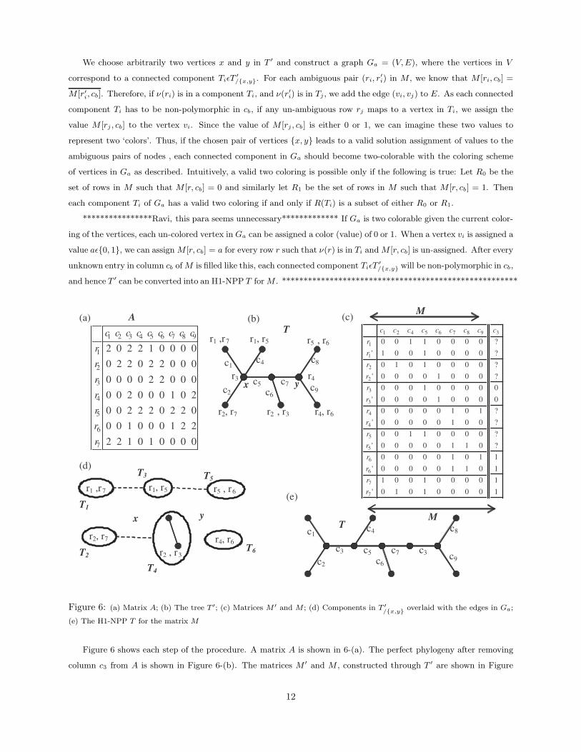
Figure 6 shows each step of the procedure. A matrix A is shown in 6-(a). The perfect phylogeny after removing
column c3 from A is shown in Figure 6-(b). The matrices M ′ and M , constructed through T ′ are shown in Figure
12
6-(c). The components in T ′/{x,y} are shown in Figure 6-(d). Since the rows r1 and r′1 in M form an ambiguous pair,
components T1 and T3 in Ga are connected. Similarly, components T2 and T4 will be connected due to the ambiguous
pair (r2, r′2, and components T3 and T5 are connected due to ambiguous pair (r5, r
′5). These edges are shown using
dashed lines in Figure 6-(d). Though the rows r4 and r′4 also form an ambiguous pair, no edge is added to Ga since
one of them (r′4) maps to the vertex y. Since y will be expanded into two vertices y0 and y1, r′4 can map to any of
the two vertices y0 and y1, and hence the pair of rows (r4, r′4) does not impose any restriction on the coloring of the
vertices in Ga. Components T1, T2, T5 and T6 can similarly be assigned a color of 1 because of the rows r7, r′7, r′6
and r6, respectively. T3 and T4 can not directly be assigned any color, since no unambiguous row maps to them. It
can be seen that Ga is two-colorable, and the only possible coloring is to assign color 0 to both T3 and T4. The final
H1-NPP T is shown Figure 6-(e).
The fundamental problem now is how to find the two sites x and y in T ′. In case of the H1-NPP problem in
Section 2, the conflict graph Gc could be constructed, RMP could be deduced from Gc, and the two vertices x and y
could be directly selected as the terminal ends of RMP. In case of the H1-NPPH problem, since we can not construct
the conflict graph completely (unless in very obvious special scenarios), we must exhaustively search for the vertices
by checking each pair of vertices in T ′. Since there are exactly m vertices in T ′, there will O(m2) pairs of vertices
that we need to check.
For each pair of vertices, the graph Ga can be constructed in O(n + m) time, allowing parallel edges. Since there
are at most O(n) edges in Ga (at most one for each row in A), the connected components in Ga can be identified
in O(n + m) time using depth-first search. Two-coloring of Ga can be obtained in O(n+m) time using breadth-first
search. Hence, the overall complexity of the algorithm is O(m2(n + m)).
3.2 Making use of the conflict graph
The conflict graph provides useful information that can be utilized to speed up the above algorithm. Even though
it might not be possible to build the conflict graph completely, we can make use of what is available of the conflict
graph in order to reduce the O(m2) search space of the pairs of vertices.
Inferring the recombination path
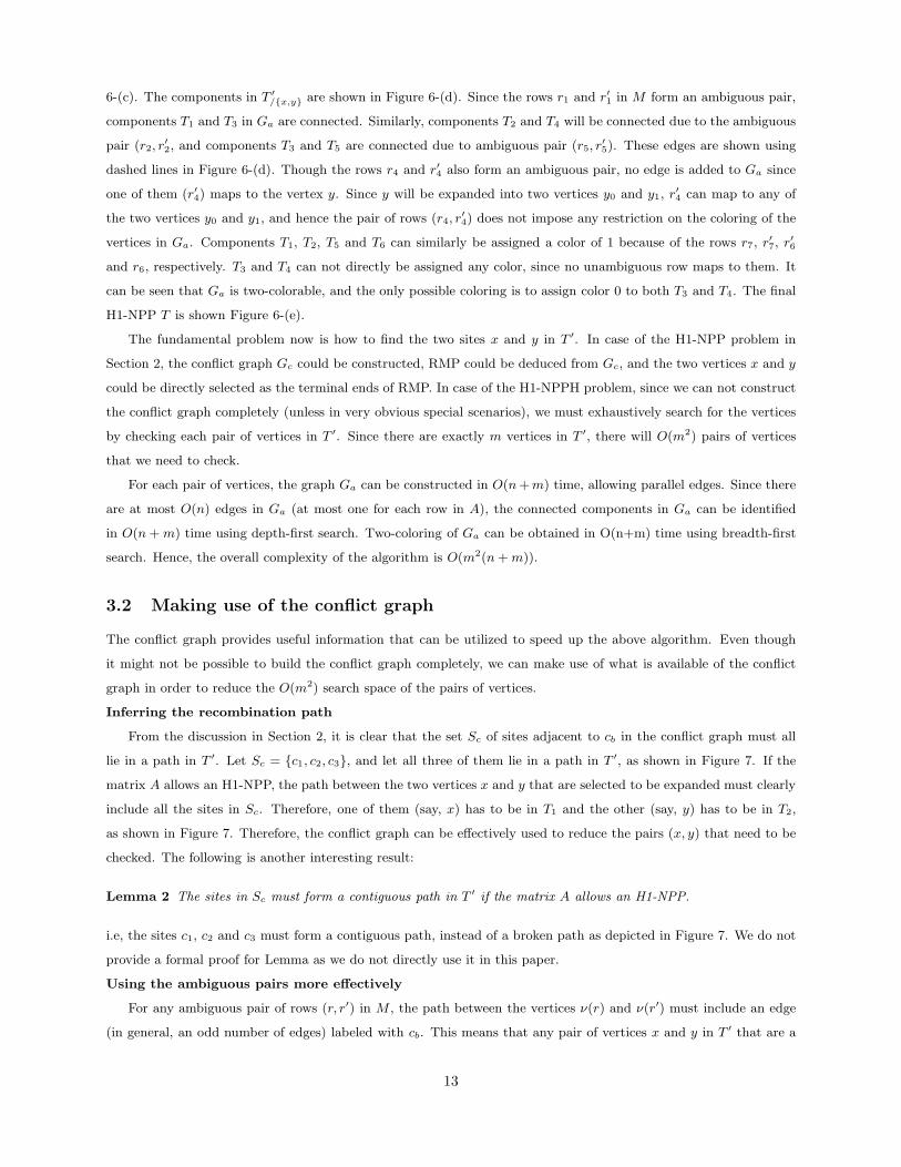
From the discussion in Section 2, it is clear that the set Sc of sites adjacent to cb in the conflict graph must all
lie in a path in T ′. Let Sc = {c1, c2, c3}, and let all three of them lie in a path in T ′, as shown in Figure 7. If the
matrix A allows an H1-NPP, the path between the two vertices x and y that are selected to be expanded must clearly
include all the sites in Sc. Therefore, one of them (say, x) has to be in T1 and the other (say, y) has to be in T2,
as shown in Figure 7. Therefore, the conflict graph can be effectively used to reduce the pairs (x, y) that need to be
checked. The following is another interesting result:
Lemma 2 The sites in Sc must form a contiguous path in T ′ if the matrix A allows an H1-NPP.
i.e, the sites c1, c2 and c3 must form a contiguous path, instead of a broken path as depicted in Figure 7. We do not
provide a formal proof for Lemma as we do not directly use it in this paper.
Using the ambiguous pairs more effectively
For any ambiguous pair of rows (r, r′) in M , the path between the vertices ν(r) and ν(r′) must include an edge
(in general, an odd number of edges) labeled with cb. This means that any pair of vertices x and y in T ′ that are a
13
c1 c3
u u� v� v
T�
c2
T1 T2
Figure 7: Any solution must involve a vertex from T1 and a vertex from T2
possible solution must be such that ν(r) and ν(r′) are not in the same connected component TiǫT′/{x,y}. The following
lemma states this property formally:
Lemma 3 For any two vertices x and y in T ′ that can be expanded to form a H1-NPPH solution for matrix A, the
path between the vertices ν(r) and ν(r′) for every ambiguous pair (r, r′) must include the vertex x or y or both.
Proof Let there be an ambiguous pair (r, r′) in M so that the path in T ′ between the two vertices ν(r) and ν(r′)
does not include the vertices x or y or both. This means that the vertices ν(r) and ν(r) are in the same connected
component TiǫT′/{x,y}. Since M [r, cb] = M [r′, cb], this implies that Ti can not be non-polymorphic with respect to cb.
Hence, there must be an edge within Ti labeled with cb in addition to the two edges labeled with cb inserted at the
vertices x and y. Hence the two vertices x and y can not lead to an H1-NPP solution for the matrix A. Therefore, for
any pair of vertices x and y in T ′ that can be expanded into an H1-NPPH solution for matrix A, the path between
the vertices ν(r) and ν(r′) for every ambiguous pair (r, r′) must include the vertex x or y or both. ♦
Lemma 3 can be used to avoid checking some vertex pairs. Let R be the set of rows in A such that A[r, cb] = 2
for every rǫR. Let Rx ⊆ R be the set of rows in A such that, for every rǫRy, the path between the vertices ν(r) and
ν(r′) in T ′ includes the vertex x in T ′. Similarly, let Ry be the corresponding set of rows for the vertex y in T ′. The
pair of vertices x and y can not be a solution unless R = Rx
⋃Ry .
3.3 The H(1, q)-NPPH problem
The solution for the H(1, q)-NPPH problem is a simple extension to the solution for the H1-NPPH problem. All the
discussion above applies to H(1, q)-NPPH problem, with the only difference being that instead of finding a pair of
vertices x and y, we need to find a set of q + 1 vertices S so that T ′ can be converted into an H(1, q)-NPP T by
expanding each one of q + 1 vertices in S into an edge labeled with cb.
In case of the H(1, q)-NPP problem, we could use Gc to narrow down the possible sets of vertices for S . We can
not do the same thing here, since Gc is not complete. Therefore, we need to try all-possible sets of vertices of size q+1.
There are (mq+1) such possible sets of vertices. For each set, testing if the set of vertices form a solution is identical
to the procedure for the H1-NPPH problem - we build the graph Ga in which each vertex represents a connected
component in T ′/S . As before, we two vertices vi and vi have an edge between them if there is an ambiguous pair (r, r′)
in M so that the vertex ν(r) is in vi and the vertex ν(r′) is in vj . We need to test if the graph Ga is two-colorable.
As in the case of the H(1, q)-NPP problem, This algorithm can be implemented to run in O(nm2 + mq+1(n + m)
time.
14
3.4 The H(p, q)-NPPH problem
The solution to the H(p, q)-NPPH problem is an obvious extension of the H(1, q)-NPPH problem. We first need to
find a set of p columns C so that the matrix A′ obtained by removing the columns in C from A has a perfect phylogeny
T ′. Once T ′ is constructed, we can essentially treat the problem as p H(1, q)-NPPH problems. The time complexity
of the algorithm is O(nmp+1 + ηpmq+1(n + m)), where η is the number distinct sets of vertices C such that removing
the sites C from A results in a perfect phylogeny.
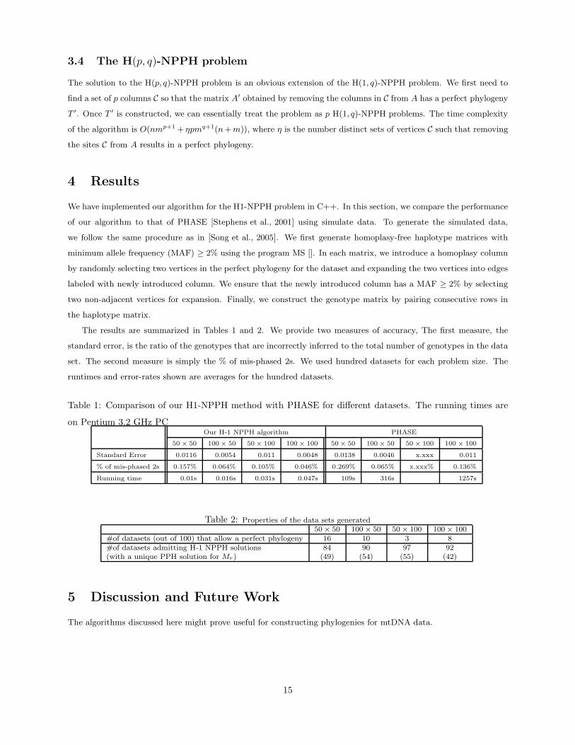
4 Results
We have implemented our algorithm for the H1-NPPH problem in C++. In this section, we compare the performance
of our algorithm to that of PHASE [Stephens et al., 2001] using simulate data. To generate the simulated data,
we follow the same procedure as in [Song et al., 2005]. We first generate homoplasy-free haplotype matrices with
minimum allele frequency (MAF) ≥ 2% using the program MS []. In each matrix, we introduce a homoplasy column
by randomly selecting two vertices in the perfect phylogeny for the dataset and expanding the two vertices into edges
labeled with newly introduced column. We ensure that the newly introduced column has a MAF ≥ 2% by selecting
two non-adjacent vertices for expansion. Finally, we construct the genotype matrix by pairing consecutive rows in
the haplotype matrix.
The results are summarized in Tables 1 and 2. We provide two measures of accuracy, The first measure, the
standard error, is the ratio of the genotypes that are incorrectly inferred to the total number of genotypes in the data
set. The second measure is simply the % of mis-phased 2s. We used hundred datasets for each problem size. The
runtimes and error-rates shown are averages for the hundred datasets.
Table 1: Comparison of our H1-NPPH method with PHASE for different datasets. The running times are
on Pentium 3.2 GHz PCOur H-1 NPPH algorithm PHASE
50 × 50 100× 50 50× 100 100× 100 50× 50 100× 50 50 × 100 100 × 100
Standard Error 0.0116 0.0054 0.011 0.0048 0.0138 0.0046 x.xxx 0.011
% of mis-phased 2s 0.157% 0.064% 0.105% 0.046% 0.269% 0.065% x.xxx% 0.136%
Running time 0.01s 0.016s 0.031s 0.047s 109s 316s 1257s
Table 2: Properties of the data sets generated50 × 50 100 × 50 50 × 100 100 × 100
#of datasets (out of 100) that allow a perfect phylogeny 16 10 3 8#of datasets admitting H-1 NPPH solutions 84 90 97 92(with a unique PPH solution for Mr) (49) (54) (55) (42)
5 Discussion and Future Work
The algorithms discussed here might prove useful for constructing phylogenies for mtDNA data.
15
References
[Bafna et al., 2002] Bafna, V., Gusfield, D., Lancia, G., and Yooseph, S. (2002). Haplotyping as perfect phylogeny: A directapproach. Technical Report CSE-2002-21, Department of Computer Science, The University of California at Davis.
[Bonizzoni et al., 2003] Bonizzoni, P., Vedova, G. D., Dondi, R., and Li, J. (2003). The haplotyping problem: And overview ofcomputational models and solutions. Journal of Computer Scienc and Technology, 18(6):675–688.
[Chung and Gusfield, 2002] Chung, R. H. and Gusfield, D. (2002). Pph - a program for deducing haplotypes that fit a perfectphylogeny. Technical Report CSE-2002-27, Department of Computer Science, The University of California at Davis.
[Clark, 1990] Clark, A. G. (1990). Inference of haplotypes from pcr-amplified samples of diploid populations. Mol. Biol. Evol.,7:111–122.
[Ding et al., 2005] Ding, Z., Filkov, V., and Gusfield, D. (2005). A linear time algorithm for the perfect phylogeny haplotyping(pph) problem. In Proceedings of RECOMB, MIT, Cambridge, MA.
[Eskin et al., 2003] Eskin, E., Halperin, E., and Karp, R. M. (2003). Large scale reconstruction of haplotypes from genotypedata. In Proceedings of RECOMB.
[Fernandez-Baca and Lagergren, 2003] Fernandez-Baca, D. and Lagergren, J. (2003). A polynomial time algorithm for near-perfect-phylogeny. SIAM Journal of Computing, 32(5):1115–1127.
[Gusfield, 2002] Gusfield, D. (2002). Haplotyping as perfect phylogeny: conceptual framework and efficient solutions. InProceedings of RECOMB.
[Gusfield et al., 2003] Gusfield, D., Eddhu, S., and Langley, C. (2003). Efficient reconstruction of phylogenetic networks withconstrained recombination. In Proceedings of CSB2003, pages 363–374, Stanford, CA.
[Halperin and Karp, 2004] Halperin, E. and Karp, R. (2004). Perfect phylogeny and haplotype assignment. In Proceedings ofRECOMB.
[HapMapConsortium, 2003] HapMapConsortium (2003). The international hapmap project. Nature, 426:789–796.
[Hudson and Kaplan, 1985] Hudson, R. and Kaplan, N. (1985). Statistical propertied of the number of recombination eventsin the history of a sample of dna sequences. Genetics, 111:147–165.
[Kimmel and Shamir, 2005] Kimmel, G. and Shamir, R. (2005). The incomplete perfect phylogeny problem. J BioinformComput Biol., 3(2):1–25.
[Liu and Zhang, 2004] Liu, Y. and Zhang, C.-Q. (2004). A linear solution for haplotype perfect phylogeny problem. InInternational Conference on Bioinformatics and its Applications (ICBA), Nova Southeastern University, Fort Lauderdale,USA.
[Song et al., 2005] Song, Y. S., Wu, Y., and Gusfield, D. (2005). Algorithms for imperfect phylogeny haplotyping (ipph) witha single homoplasy or recombination event. In Proceedings of WABI 2005, pages 152–164.
[Stephens et al., 2001] Stephens, M., Smith, N., and Donnelly, P. (2001). A new statistical method for haplotype reconstructionfrom population data. Am J Hum Genet., 68.
[VijayaSatya and Mukherjee, 2005a] VijayaSatya, R. and Mukherjee, A. (2005a). An efficient algorithm for perfect phylogenyhaplotyping. In Proceedings of CSB2003, pages 103–110, Stanford, CA.
[VijayaSatya and Mukherjee, 2006] VijayaSatya, R. and Mukherjee, A. (2006). An optimal algorithm for perfect phylogenyhaplotyping. to appear in the Journal of Computational Biology.
[VijayaSatya and Mukherjee, 2005b] VijayaSatya, R. and Mukherjee, A. (December 12, 2005b). The undirected incompleteperfect phylogeny problem. Technical Report CS-TR-05-11, School of Computer Science, University of Central Florida,Orlando.
16


