A

Contextual tag inferenceMICHAEL I. MANDEL, RAZVAN PASCANU, DOUGLAS ECK, and YOSHUA BENGIO, Universite deMontrealLUCA M. AIELLO and ROSSANO SCHIFANELLA, Universita di Torinoand FILIPPO MENCZER, Indiana University

This paper examines the use of two kinds of context to improve the results of content-based music taggers: the relationshipsbetween tags and between the clips of songs that are tagged. We show that users agree more on tags applied to clips temporally

”closer” to one another; that conditional restricted Boltzmann machine models of tags can more accurately predict related tagswhen they take context into account; and that when training data is ”smoothed” using context, support vector machines can

better rank these clips according to the original, unsmoothed tags and do this more accurately than three standard multi-label

classifiers.

Categories and Subject Descriptors: H.1.2 [Information Systems]: Models and Principles—Human information processing;H.5.5 [Information Interfaces and Presentation]: Sound and Music Computing—Signal analysis, synthesis, and processing;I.2.6 [Artificial Intelligence]: Learning—Connectionism and neural nets

General Terms: Experimentation, Performance

Additional Key Words and Phrases: Autotagging, clips, context, music, smoothing, tags

ACM Reference Format:ACM Trans. Multimedia Comput. Commun. Appl. V, N, Article A (September 10), 17 pages.DOI = 10.1145/0000000.0000000 http://doi.acm.org/10.1145/0000000.0000000

1. INTRODUCTION

The amount of digital music available online is vast and increasing, not just as official releases onrecord labels, but also as user generated content. Social tags and expert generated tag descriptionsallow users to find relevant content on Last.fm and Pandora.com, respectively, but they are timeconsuming and expensive to collect. This paper discusses methods for automatically applying tags tomusic (“autotagging”) to scale these data beyond the limitations of current manual processes.

Automatically generated tags can be used in three primary ways. They can be used to search bydescription through a collection of music that has been automatically described. For example, a usermight want to find music that is “folk rock with male vocals and acoustic guitar.” They can be used tobrowse through music with similar descriptions. For example, the same search could be constructed for auser automatically from David Bowie’s “Space Oddity,” without having to articulate a specific description.

Author’s address: M. Mandel: University of Montreal, Department of Computer Science and Operations Research, CP 6128, Succ.Centre-Ville, Montreal, Quebec, H3C 3J7 CANADAPermission to make digital or hard copies of part or all of this work for personal or classroom use is granted without fee providedthat copies are not made or distributed for profit or commercial advantage and that copies show this notice on the first pageor initial screen of a display along with the full citation. Copyrights for components of this work owned by others than ACMmust be honored. Abstracting with credit is permitted. To copy otherwise, to republish, to post on servers, to redistribute tolists, or to use any component of this work in other works requires prior specific permission and/or a fee. Permissions may berequested from Publications Dept., ACM, Inc., 2 Penn Plaza, Suite 701, New York, NY 10121-0701 USA, fax +1 (212) 869-0481, orpermissions@acm.org.c© 10 ACM 1551-6857/10/09-ARTA $10.00

DOI 10.1145/0000000.0000000 http://doi.acm.org/10.1145/0000000.0000000

ACM Transactions on Multimedia Computing, Communications and Applications, Vol. V, No. N, Article A, Publication date: September 10.

A:2 • Michael Mandel et al.

Finally, they allow summarization of search results and other collections of music. Descriptions ofminutes or hours of music can be skimmed in seconds from which relevant candidates can be selectedfor more thorough auditory screening.

This paper specifically discusses ways of taking context into account for improving autotagger trainingdata. Context in this case means some combination of the relationships between tags and the relation-ships between 10-second clips of songs. Autotagging systems typically treat each tag as an independentclassification problem, and each clip of music as an independent data point. The models described in thiswork take advantage of the relationships between tags and between clips to make better predictions oftags.

After discussing previous work on autotagging and context in machine vision in Section 1.1, Sec-tion 2 describes measurements of temporal context in an existing dataset. Section 2.1 then describeswhat is to our knowledge the first use of Amazon’s Mechanical Turk service to collect autotaggingtraining data, and another examination of temporal context on these data. Section 3 then describesthe various language models employed to capture tag-tag contextual relationships, specifically, therestricted Boltzmann machine (RBM), the conditional RBM (CRBM), and the doubly conditional RBM(DCRBM), and information theoretic models of tag-tag similarity. Finally, Section 4 describes fourexperiments conducted with these models on three different datasets, measuring their prediction of thetags themselves and the improvement that they impart to support vector machine-based autotaggers.

1.1 Background

Researchers have investigated a number of music autotagging techniques over the last decade [Slaney2002; Whitman and Rifkin 2002; Eck et al. 2008; Tingle et al. 2010]. Many current autotagging systems(e.g. [Mandel and Ellis 2008]) treat each tag as a separate classification or ranking problem. This papergeneralizes this to the problem of predicting the presence or relevance of multiple tags simultaneously,which is known as multi-label classification [Tsoumakas et al. 2010]. Many multi-label classificationalgorithms have been proposed in the literature [Boutell et al. 2004; Kang et al. 2006; Tsoumakas andVlahavas 2007; Zhang and Zhou 2007; Han et al. 2010], including some explicitly designed for problemsin music [Trohidis et al. 2008].

One form of context that we explore in this paper is the exploitation of the relationships betweentags. This form of context has been explored by other authors with regards to music tagging, generallyas a second stage on top of independent tag predictors. Aucouturier et al. [2007] use a decision treelearned from ground truth tags to enforce certain relationships between tag predictions and find thatit improves the precision of their taggers by an average of 5% and up to 15%. Bertin-Mahieux et al.[2008] use a second layer of boosting on top of the individual autotaggers, but do not show a significantimprovement over the individual autotaggers. Miotto et al. [2010] use a Dirichlet mixture model tosmooth autotagger outputs, improving the performance of acoustic classifiers and outperforming asupport vector machine context model under a number of metrics.

The context model of Miotto et al. [2010] is inspired by context models from the vision literature,specifically, Rasiwasia and Vasconcelos [2009]. The vision and image retrieval literature in general hasdeveloped rather sophisticated notions of context that could be applied to music, such as Chen et al.[2010]. Heitz and Koller [2008] characterize these different types of context well, describing their ownwork as “stuff-thing” context, meaning that it uses background textures to inform its predictions ofthe identities of foreground objects. This is contrasted against the “scene-thing” context of Murphyet al. [2004], which first uses the “gist” of the image to classify the scene (e.g. office, hallway, street),and then uses the scene predictions to inform priors on where and what objects should be expected.Rabinovich et al. [2007] use a “thing-thing” context, where the identities of objects in scenes informone another. This is perhaps the most similar of the three to the context used in music tagging. OtherACM Transactions on Multimedia Computing, Communications and Applications, Vol. V, No. N, Article A, Publication date: September 10.

Contextual tag inference • A:3

visual contexts include the 3D geometric relationships between objects [Hoiem et al. 2008] and therelationship between human pose and objects like sports equipment [Yao and Fei-Fei 2010]. In both ofthese cases, object identification and context mutually reinforce each other.

These different types of visual context could have analogs in music. For example, a visual scene mightbe analogous to a musical genre, as the priors over instruments, moods, etc. found in a song shoulddepend on the genre of the song. Just as an office scene has a high probability of including a computerkeyboard [Murphy et al. 2004], a rock song has a high probability of involving guitar. Similarly, justas a street scene has a low prior on that same keyboard, a hip-hop song has a low prior on that sameguitar. In the same way, spatial context in images could correspond to temporal context in music andthe 3D geometric context of Hoiem et al. [2008] might correspond to a more nuanced notion of musicalstructural context. Just as Hoiem et al. [2008] infer the 3D geometry of a scene from a 2D projection ofit and use it to perform better spatial reasoning about car and pedestrian detection, so might musicalstructure be inferred from the temporal and musical surfaces and used to better inform tagging. Thispaper will, however, restrict itself to a simpler notion of temporal context, defined simply according toclip metadata: its offset into a track, the track, the album, and the artist. In fact, many of our models willonly consider the clip and track identities. While this is greatly simplified, it is still useful in modelingthe temporal context of music and tags.

Our examination of the relationships between the tags of different parts of the same song was enabledby our collection of a new dataset using Amazon.com’s Mechanical Turk service. Mechanical Turk isa marketplace where “requesters” post tasks that require some amount of basic human intelligencealong with a bounty for their completion. For example, we paid “turkers” $0.03-0.05 per clip that theyannotated with 5-10 tags. This marketplace allowed us to gather a new dataset relatively quickly andcheaply using 5 clips from each song. Mechanical Turk has been used in the past for collecting naturallanguage processing data [Snow et al. 2008] and vision data [Sorokin and Forsyth 2008; Whitehill et al.2009], but to our knowledge it has not been used for collecting tag data for music. Concurrently withour work, Lee [2010] used Mechanical Turk to collect music similarity judgements.

This paper is based on work presented in our previous conference publication [Mandel et al. 2010]and uses techniques described by Schifanella et al. [2010]. It applies the information theory-basedsmoothing methods of the latter with the autotaggers of the former, and adds to this a new RBM-basedsmoothing model. It also unifies the experiments presented in those papers and explicitly states theideas of context in music.

2. TEMPORAL TAG CONTEXT

How similar are the tags that different users apply to the same clip? Different clips from the sametrack? Clips from different tracks on the same album? Clips from different albums from the sameartist? Clips from different artists? How does this similarity vary for clips from the same track asthe separation between the clips increases? We consider these questions and attempt to answer themthrough a simple co-occurrence analysis of tags similar to the one performed by Schifanella et al. [2010].This investigation of temporal context or the temporal “scale” of various tags and types of tags willinform our tag language models.

Our existing MajorMiner dataset [Mandel and Ellis 2008] provides an excellent testbed for examiningmany of these questions. In order to perform this analysis, we measured the number of co-occurring tagsin every pair of (user,clip) observations. We categorized each pair of observations by the relationshipsbetween the users and the clips. For example, they could be from the same user, and the clips couldbe from different tracks on the same album. Or they could be from different users but the same clip.We then simply took the average number of co-occurring clips for each of these various categorizations.Figure 1(a) shows the results of this analysis.

ACM Transactions on Multimedia Computing, Communications and Applications, Vol. V, No. N, Article A, Publication date: September 10.

A:4 • Michael Mandel et al.

Nothing Artist Album Track ClipShared

0.0

0.2

0.4

0.6

0.8

1.0

1.2

Co-o

ccurr

ing t

ags

60 40 20 0 20 40 60Separation (% of track)

0.40

0.45

0.50

0.55

0.60

0.65

Co-o

ccurr

ing t

ags

above b

ase

line

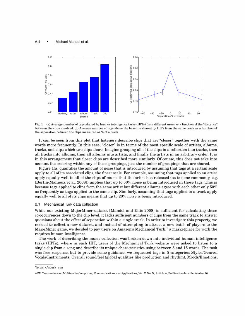
Fig. 1. (a) Average number of tags shared by human intelligence tasks (HITs) from different users as a function of the “distance”between the clips involved. (b) Average number of tags above the baseline shared by HITs from the same track as a function ofthe separation between the clips measured as % of a track.

It can be seen from this plot that listeners describe clips that are “closer” together with the samewords more frequently. In this case, “closer” is in terms of the most specific scale of artists, albums,tracks, and clips which two clips share. Imagine grouping all of the clips in a collection into tracks, thenall tracks into albums, then all albums into artists, and finally the artists in an arbitrary order. It isin this arrangement that closer clips are described more similarly. Of course, this does not take intoaccount the ordering within any of these groupings, just the number of groupings that are shared.

Figure 1(a) quantifies the amount of noise that is introduced by assuming that tags at a certain scaleapply to all of its associated clips, the finest scale. For example, assuming that tags applied to an artistapply equally well to all of the clips of music that the artist has released (as is done commonly, e.g.[Bertin-Mahieux et al. 2008]) implies that up to 50% noise is being introduced in those tags. This isbecause tags applied to clips from the same artist but different albums agree with each other only 50%as frequently as tags applied to the same clip. Similarly, assuming that tags applied to a track applyequally well to all of its clips means that up to 20% noise is being introduced.

2.1 Mechanical Turk data collection

While our existing MajorMiner dataset [Mandel and Ellis 2008] is sufficient for calculating theseco-occurrences down to the clip level, it lacks sufficient numbers of clips from the same track to answerquestions about the effect of separation within a single track. In order to investigate this property, weneeded to collect a new dataset, and instead of attempting to attract a new batch of players to theMajorMiner game, we decided to pay users on Amazon’s Mechanical Turk,1 a marketplace for work therequires human intelligence.

The work of describing the music collection was broken down into individual human intelligencetasks (HITs), where in each HIT, users of the Mechanical Turk website were asked to listen to asingle clip from a song and describe its unique characteristics using between 5 and 15 words. The taskwas free response, but to provide some guidance, we requested tags in 5 categories: Styles/Genres,Vocals/Instruments, Overall sound/feel (global qualities like production and rhythm), Moods/Emotions,

1http://mturk.com

ACM Transactions on Multimedia Computing, Communications and Applications, Vol. V, No. N, Article A, Publication date: September 10.

Contextual tag inference • A:5

and Other (sound alike artists, era, locale, song section, audience, activities, etc.). In order to avoidbiasing the turkers’ responses, no examples of tags were provided. Turkers were paid between $0.03and $0.05 per clip, on which they generally spent about one minute.

The music used in the experiment was collected from music blogs that are indexed by the HypeMachine.2 We downloaded the front page of each of the approximately 2000 blogs and recorded theURLs of any mp3 files linked from them, a total of approximately 17,000 mp3s. We downloaded 1500 ofthese mp3s at random, of which approximately 700 were available, error free, and at least 128 kbpswhile still being below 10 megabytes (to avoid DJ sets, podcasts, etc). Of these, we selected 185 atrandom. From each of these 185 tracks, we extracted five 10-second clips evenly spaced throughoutthe track. We presented these clips to turkers in a random order, and generally multiple clips from thesame track were not available simultaneously. Each clip was seen by 3 different turkers.

Mechanical Turk gives the “requester” the opportunity to accept or reject completed HITs eithermanually or automatically. In order to avoid spammers, we designed a number of rules for automaticallyrejecting HITs based on analyses of each and all of a user’s HITs. Individual HITs were rejected if: (1)they had fewer than 5 tags, (2) a tag had more than 25 characters, or (3) less than half of the tags werefound in a dictionary of Last.fm tags. All of a users’ HITs were rejected if: (1) that user had a very smallvocabulary compared to the number of HITs they performed (fewer than 1 unique tag per HIT), (2) theyused any tag too frequently (4 tags were used in more than half of their HITs), (3) they used more than15% “stop words” like nice, music, genre, etc., or (4) at least half of their HITs were rejected for otherreasons. The list of stop words was assembled by hand from HITs that were deemed to be spam.

We posted a total of 925 clips, each of which was to be seen by 3 turkers for a total of 2775 HITs. Weaccepted 2566 completed HITs and rejected 305 HITs. Some of the rejected HITs were re-posted andothers were never completed. The completed HITs included 15,500 (user, tag, clip) triples from 209unique turkers who provided 2100 unique tags. Of these tags, 113 were used by at least 10 turkers,making up 13,000 of the (user, tag, clip) triples. We paid approximately $100 for these data, althoughthis number doesn’t include additional rounds of data collection and questionnaire tuning.

2.1.1 Results. The data from Mechanical Turk provide an in-depth look at the relationships betweentags applied to clips in the same track. Figure 1(b) shows the normalized number of tag co-occurrencesfor clips with different separations (in terms of percentage of the track). The normalization consists ofcalculating the difference between the number of tags that co-occur for clips at a particular offset in thesame track versus those in different tracks. This normalization is necessary because different offsetsinto tracks were generally heard by different turkers with their own idiosyncratic vocabularies. Withthis normalization, it can be seen that there is a monotonic fall-off of tag co-occurrence from a peak at a0% offset, supporting the data in Figure 1(a).

3. TAG LANGUAGE MODELS

Tags collected from human users are typically quite sparse. With Mechanical Turk, we were able tocollect tags for a small number of clips, each seen by 3 people with 17 (user, tag) pairs on average.With the MajorMiner game, we were able to collect tags for a slightly larger number of clips, each seenby about 7 people with 30 (user, tag) pairs on average. The Last.fm dataset that we are using (seeSection 4.1) has over 1.2 million tracks and 8.5 million (user, tag, track) triples, making an average ofonly 7 (user, tag) pairs per track. Additionally, because popular songs are tagged much more frequentlythan less popular songs, only 18% of songs have more than 7 (user, tag) pairs applied to them.

2http://hypem.com/list

ACM Transactions on Multimedia Computing, Communications and Applications, Vol. V, No. N, Article A, Publication date: September 10.

A:6 • Michael Mandel et al.

For the popular tracks, it is not a problem to count the number of times each tag has been applied toeach clip, but for those 82% of tracks in the long tail, these tag data are quite noisy. One approach toremoving this noise is by treating the true tags as hidden data and inferring them from the observationsof tags that were applied. Such a tag language model should be able to identify both tags that shouldhave been applied, but weren’t, and tags that were applied but should not have been.

This paper discusses and tests two different kinds of tag language models, one based on an informationtheoretic formulation of this inference [Schifanella et al. 2010], and the second based on restrictedBoltzmann machines (RBMs) [Mandel et al. 2010; Mandel et al. 2011]. While there are many more usesfor it, in this case, we only use the information theoretic model to learn the relationships between tagsin a tag-tag similarity matrix. The RBM models can learn this tag-tag context, and can additionallyincorporate the temporal context discussed in Section 2 through conditioning on “auxiliary variables.”

3.1 Information theoretic models

Inferring suitable hidden tags for resources (clips, tracks, albums and so on) with poor tagging informa-tion and detecting noisy tags in the set of tags attached to a resource are tasks that can be achieved bymining the global tag-to-tag similarity relationships occurring in the folksonomy.

Given a similarity score for every pair of tags, any set of tags associated with a specific resource canbe expanded by adding the tags that are most similar to the given tags, under the assumption thattags which are strongly related to each other apply equally to the same resource. For instance, if rapand hip-hop are found to be very similar and one resource is tagged with only rap, it is very likelythat hip-hop can be applied as well. Conversely, a noisy tag set can be reduced by wiping out thosetags that are not strongly related to the majority of other tags assigned to the same resource. Here, wereport a brief overview on how tag-to-tag similarity can be computed.

A widely accepted representation of folksonomies is based on a set of triples (u, r, t) representing auser u marking a resource r with a tag t. Extracting meaningful similarity patterns occurring betweentags in such three-dimensional model requires a dimensionality reduction of the triple space, becausemeasures for relatedness and similarity are still not well developed for three-mode data. The processof reducing a folksonomy to a two-mode relationship is known as aggregation [Markines et al. 2009].Although the aggregation could be performed across any of the three dimension involved, in our settingwe are interested in calculating the similarity between pairs of tags by means of comparing the resourcesthey annotate; for this reason we aggregate on the user dimension. Doing so we obtain a description ofeach tag as a weighted vector of resources.

As widely shown by previous work [Markines et al. 2009], the aggregation can be performed in variousways, leading to as many different calculations of the weights in the resource vector. Simple examples ofaggregation are the projection aggregation, which outputs a binary vector denoting the set of resourceslabeled by the tag, and the distributional aggregation, which produces a frequency-weighted vectorwhere resources are weighted according to how many times they have been tagged with the consideredtag.

Collapsing the two-dimensional tag-resource space into a weighted tag-to-tag relation is performed byapplying a semantic similarity measure (e.g., cosine similarity) to each pair of resource vectors. Previouswork addresses the application of different metrics in such context [Markines et al. 2009; Schifanellaet al. 2010]. Since most of these metrics leverage fundamental principles from the information theory, inthe following we will name information theoretic (or also InfTh for brevity) all the autotagging modelsthat use these metrics.ACM Transactions on Multimedia Computing, Communications and Applications, Vol. V, No. N, Article A, Publication date: September 10.

Contextual tag inference • A:7

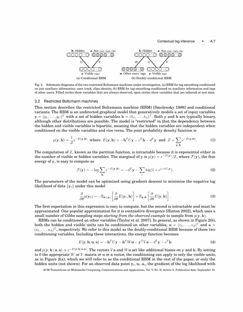
(a) Conditional RBM (b) Doubly-conditional RBM

Fig. 2. Schematic diagrams of the two restricted Boltzmann machines under investigation. (a) RBM for tag smoothing conditionedon just auxiliary information: user, track, clips identity, (b) RBM for tag smoothing conditioned on auxiliary information and tagsof other users. Filled circles show variables that are always observed, open circles show variables that are inferred at test time.

3.2 Restricted Boltzmann machines

This section describes the restricted Boltzmann machine (RBM) [Smolensky 1986] and conditionalvariants. The RBM is an undirected graphical model that generatively models a set of input variablesy = (y1, . . . , yC)

T with a set of hidden variables h = (h1, . . . , hn)T . Both y and h are typically binary,

although other distributions are possible. The model is “restricted” in that the dependency betweenthe hidden and visible variables is bipartite, meaning that the hidden variables are independent whenconditioned on the visible variables and vice versa. The joint probability density function is

p(y,h) =1

Ze−E(y,h) where E(y,h) = −hTUy − cTh− dTy and Z =

∑y,h

e−E(y,h). (1)

The computation of Z, known as the partition function, is intractable because it is exponential either inthe number of visible or hidden variables. The marginal of y is p(y) = e−F(y)/Z, where F(y), the freeenergy of y, is easy to compute as

F(y) = − log∑h

e−E(y,h) = −dTy −∑i

log(1 + eci+Uiy). (2)

The parameters of the model can be optimized using gradient descent to minimize the negative loglikelihood of data {yt} under this model

∂

∂θp(yt) = −Eh |yt

[∂

∂θE(yt,h)

]+ Ey,h

[∂

∂θE(y,h)

]. (3)

The first expectation in this expression is easy to compute, but the second is intractable and must beapproximated. One popular approximation for it is contrastive divergence [Hinton 2002], which uses asmall number of Gibbs sampling steps starting from the observed example to sample from p(y,h).

RBMs can be conditioned on other variables [Taylor et al. 2007]. In general, as shown in Figure 2(b),both the hidden and visible units can be conditioned on other variables, u = (v1, . . . , vd)

T and a =(a1, . . . , aA)

T , respectively. We refer to this model as the doubly-conditional RBM because of these twoconditioning variables. Including these interactions, the energy function becomes

E(y,h,u,a) = −hTUy − hTWu− yTV a− dTy − cTh (4)

and p(y,h |u,a) ∝ e−E(y,h,u,a). The vectors V a and Wu act like additional biases on y and h. By settingto 0 the appropriate W or V matrix or u or a vector, the conditioning can apply to only the visible units,as in Figure 2(a), which we will refer to as the conditional RBM in the rest of the paper, or only thehidden units (not shown). For an observed data point yt,ut,at, the gradient of the log likelihood with

ACM Transactions on Multimedia Computing, Communications and Applications, Vol. V, No. N, Article A, Publication date: September 10.

A:8 • Michael Mandel et al.

respect to a parameter θ becomes

∂

∂θlog p(yt |ut,at) = −Eh |yt,ut,at

[∂

∂θE(yt,h,ut,at)

]+ Ey,h |ut,at

[∂

∂θE(y,h,ut,at)

]. (5)

Salakhutdinov et al. [2007] describe a conditional RBM used for collaborative filtering in which onlythe hidden variables are conditioned on other variables. Mandel et al. [2010] describe a conditionalRBM used for modeling tags of the form of Figure 2(a), while this paper is the first to describe a doublyconditional RBM used for modeling tags.

3.3 Conditional RBM tag language model

As shown in Figure 2, both the conditional RBM and doubly-conditional RBM (DCRBM) can be usedas tag language models. Both of them use the same variables and same representations for tags,hidden representations, and auxiliary information including user, track, and clip identity. The DCRBMadditionally includes a representation of the tags that other users have applied to a particular clip.

The visible units in each RBM, y, represent the tags that have been applied to a particular clip by aparticular user in the form of a binary vector. These visible units are connected to the hidden units,h, and units representing auxiliary information about the user and clip involved, a. Specifically, eachuser is given their own auxiliary unit that indicates when it is that user applying the tags. This is aso-called “one-hot” representation of user, as only one user unit is ever 1 at a tim. Additionally, however,there are analogous representations in a for the clip that has been tagged and the track from which itcame. In this way, for example, taggings of the same clip by different users can share information, ascan taggings of different clips from the same track, and taggings of different clips by the same user. Inthe case of the DCRBM, the u vector is the average of all of the other binary tag vectors that apply tothe same clip, providing the context of the tags other users have apply to the clip. The u vector is thesame length as the y vector, but the elements of u are continuous values between 0 and 1, while theelements of y are strictly 0 or 1.

The various parameters learned by the model can capture specialized information about the relation-ships between these variables. In particular, this can be encouraged by applying an L1 or L2 prior to theW and V matrices during learning. When W and V are encouraged to be sparse, the biases d capture theoverall frequency of each tag, U captures information about the correlations between tags independentof context, and W captures the relationships between tags in other taggings of the same clip. The Vmatrix captures any deviations in relative frequency between tags due to context, for example if a usertends to favor certain tags over others or if a particular clip tends to be described with tags that wouldnormally not coincide.

After a CRBM is trained, it is used to estimate p(y |a), which provides the smoothing. This is done bydrawing samples from the distribution for each particular setting of a, i.e. for each clip. Because of itsprobabilistic formulation, the CRBM allows unobserved variables to be either imputed or marginalizedaway. In particular, it is desirable to provide smoothed tags independent of a particular user’s biases,so the user variables in a are marginalized away. Additionally, the DCRBM can be provided with anaverage of all of the tag vectors for a particular clip in u, from which it estimates p(y |a,u).

4. EXPERIMENTS

This section describes a number of experiments performed to investigate the usefulness of the variousaspects of contextual tag language models. It first describes the datasets on which the models are tested,then the features used to describe the audio, then the experiments themselves.ACM Transactions on Multimedia Computing, Communications and Applications, Vol. V, No. N, Article A, Publication date: September 10.

Contextual tag inference • A:9

4.1 Datasets

Three different datasets were employed in these experiments. They came from Mechanical Turk, theMajorMiner game, and a crawl of Last.fm, roughly corresponding to small, medium, and large sizes.

The Mechanical Turk dataset is described in Section 2.1. This dataset had 925 clips, 2100 tags, 209users, and 15,500 (user, clip, tag) triples. While it is the smallest dataset, the clips that compose itwere selected in such a way as to give the best picture of within-track tag variation. Because of its size,we treated all (user, clip, tag) triples as true for the purposes of evaluation, even those that were notverified by two users.

The medium-sized dataset comes from the MajorMiner game [Mandel and Ellis 2008]. It has 2600clips, 6700 tags, 600 users, and 80,000 (user, clip, tag) triples. This dataset gives a nice balance betweensize, diversity of music, and different scales of tagging. Its tags were collected at the clip level, and soare very specific. Because approximately 7 users saw each clip, we accept as true (clip, tag) pairs onwhich two different users agree. If only one user uses a (clip, tag) pair, we count it as an intermediatestate, neither true or false, for evaluation purposes.

The largest dataset comes from the website Last.fm. Schifanella et al. [2010] describe the design of acrawler to gather the social tags describing individual tracks in Last.fm. While this is more fine-grainedtag data than is usually collected from Last.fm (e.g. [Bertin-Mahieux et al. 2008]), it is still not at theclip level like the other two datasets. In order to evaluate clip-level classification scores, we assumedthat track-level tags applied to all of a track’s clips. In practice, we found that there was enough data tosimply select the 10-second clip from the exact center of each track to use as a representative of theentire track. While the entire dataset has 1.2 million clips, 280,000 tags, 84,000 users, and 8.6 million(user, clip, tag) triples, many of these only appear infrequently. Limiting the dataset to clips, tags, andusers that appear in 100 or more triples still retains 8900 users, 9400 tracks, 7100 tags, and 1.4 milliontriples.

We pre-processed the data by transforming tags into a canonical form. We normalized the spelling ofdecades and the word “and,” removed phrases such as “sounds like” from the beginning of tags, removedwords like “music,” “sound,” and “feel” from the ends of tags, and removed punctuation. We also stemmedeach word in the tag so that different forms of the same word would match each other, e.g. drums,drum, and drumming.

4.2 Features

We use the audio features described by Mandel and Ellis [2008], which characterize the audio’s timbreand rhythm. The features are all calculated over 10-second clips of songs. The timbral features are themean and unwrapped covariance matrix of 18-dimensional Mel frequency cepstral coefficients (MFCCs).This feature captures information about music’s production and instrumentation. It specifically ignoresmusical features like harmony and melody.

The rhythmic features could be called “envelope cepstrum.” The spectrogram is divided into a numberof frequency bands, and the FFT across time is taken of each band, yielding the modulation of each band.The low frequency modulations are kept (up to 10 Hz), the log magnitude is taken, and then the DCTalong time is taken, yielding the “envelope cepstrum” in the different frequency bands. These bands arethen stacked on top of one another to create a 200-dimensional rhythmic feature vector. These featurescapture information about the music’s beat, tempo, and rhythm, attempting to separate the varioussignals from the drum kit: bass drum, snare, and hi-hat cymbal.

Both of these features are computed over all of the clips in the dataset and then normalized so thateach dimension has zero mean and unit variance. Each datapoint’s feature vector is then normalizedagain so that it has unit norm. This second normalization minimizes the number of outliers caused

ACM Transactions on Multimedia Computing, Communications and Applications, Vol. V, No. N, Article A, Publication date: September 10.

A:10 • Michael Mandel et al.

by the heavy tails of the feature dimension distributions, preventing them from dominating distancecalculations.

4.3 Experiment 1: predicting tags from context

This experiment investigates the predictive power of the various language models for tags and theadvantages that context provides for these models. It is purely textual in that it does not involve theaudio of the music at all, just the tags, tagging information, user information, and music metadata.

All three of the datasets described in Section 4.1 can be used in a leave-one-out tag prediction task.In this task, the relative probability of a novel observation is compared to that of the same observationwith one bit flipped (one tag added or deleted). If the model has captured important structure in thedata, then it will judge the true observation to be more likely than the bit-flipped version of it. Thisratio is directly connected to the so-called pseudo-likelihood of the test set [Besag 1975]. Because it isa ratio of probabilities, it does not require the computation of the partition function, Z, which is verycomputationally intensive. Mathematically, the pseudo-likelihood is defined as

PL(v | a) ≡∏i

p(vi | v\i, a) =∏i

p(v | a)p(v | a) + p(vi | a)

(6)

where vi is the ith visible unit, v\i is all of the visible units except for the ith unit, and vi is theobservation v with the ith bit flipped. Even though our observation vectors are generally very sparse(∼4% of the bits were 1s), the 1s are more important than the 0s, so we compute the average logpseudo-likelihood over the 1s and 0s separately and then average those two numbers together. Thisprovides a better indication of whether the model can properly account for the tags that are present,and diminishes the importance of the tags that aren’t present.

This leave-one-out tag prediction can be done with any model that computes the likelihood of tags.Thus we can train models with different combinations of auxiliary variables, or different structuresentirely, as long as they can predict the likelihood of novel data. A baseline comparison to all of ourRBMs is a factored model that estimates the probability of each tag independently from training dataand then measures the likelihood of each tag independently on test data. Because of the independenceof the variables, in this case the pseudo-likelihood is identical to the true likelihood.

We performed this experiment with the textual component of these three datasets, dividing the data60-20-20 into training, validation, and test sets. The observations were shuffled, but then rearrangedslightly to ensure that all of the auxiliary classes appeared at least once in the training set to avoid“out-of-vocabulary” problems. This experiment only used the singly-conditional RBM for clarity, asthe doubly-conditional RBM has very different pseudo-likelihoods due to its being conditioned on tagdata. We ran a grid search over the number of hidden units, the learning rate, and the regularizationcoefficients using only the track-based auxiliary variables, those with the most even coverage. This gridsearch involved training approximately 500 different models, each taking 10 minutes on average. Weselected the system with the best hyperparameters based on the pseudo-likelihood of the validationdataset. Once we had selected reasonable hyperparameters, we ran experiments using all combinationsof the auxiliary variables with the other hyperparameters held constant. Five different random divisionsof the data allowed the computation of standard errors.

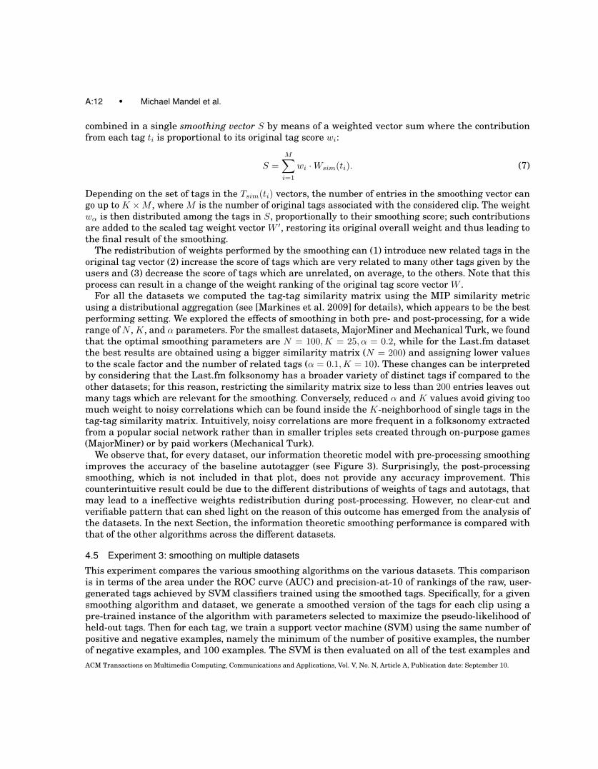
The log pseudo-likelihoods of the test datasets under these systems are shown in Table I. Theresults are not strictly comparable across datasets because they involved slightly different numbers ofvisible units. The results are shown on a per-bit basis, however, to facilitate comparison. These resultsshow first that non-conditional restricted Boltzmann machines (rows with three −s) are much moreeffective than the factored models at modeling test data. This is because in addition to modeling therelative frequencies of tags, the RBM models the relationships between tags through its hidden units.ACM Transactions on Multimedia Computing, Communications and Applications, Vol. V, No. N, Article A, Publication date: September 10.

Contextual tag inference • A:11

Table I. Average per-bit log pseudo-likelihood (lessnegative is better) for restricted Boltzmann machines

conditioned on different types of auxiliaryinformation. A + indicates that the auxiliary

information was present, a − indicates that it wasabsent. The baseline system is a factored model

evaluated in the same way.

Auxiliary infoDataset User Track Clip log(PL)±stderr

MajorMiner + + + −0.9179±0.0088

MajorMiner + + − −0.9189±0.0070

MajorMiner + − − −0.9416±0.0074MajorMiner − − − −1.0431±0.0095

MajorMiner baseline −1.4029±0.0024

Mech. Turk + + − −0.893 ± 0.015Mech. Turk + − − −0.904 ± 0.013

Mech. Turk + + + −0.914 ± 0.012

Mech. Turk − − − −1.039 ± 0.013Mech. Turk baseline −1.300 ± 0.007

Conditioning the RBM on auxiliary information (rows with at least one +) further improves the pseudo-likelihoods. Specifically, it seems that the most useful auxiliary variable is the identity of the user,but the identity of the track helps as well. Including clip information is slightly detrimental, althoughnot statistically significantly so, possibly because it introduces a large number of extra parameters toestimate in the Wa matrix from few observations.

4.4 Experiment 2: information theoretic smoothing

It is possible to exploit the tag-tag similarity relationship derived from the information theoretic modeldefined in Section 3.1 to improve the autotagger’s prediction accuracy through a process of remodulationof the tag scores that we call smoothing. The idea behind this kind of smoothing is that the weightedtag vectors can be remodulated through a redistribution of scores to increase the weight of the mostrelevant tags and to minimize those of the noisy ones.

The smoothing procedure can be reasonably applied in pre-processing on the tag vectors used in thelearning set as well as in post-processing on the autotagger output. Pre-smoothing is aimed at refiningthe autotagger input to improve learning when the considered clips are poorly or noisily tagged, whilepost-smoothing is used to adjust the tag prediction to highlight the most relevant tags or to bring outrelevant tags that have not been detected by the autotagger. The same smoothing algorithm is used inboth pre-processing and post-processing phases, modulo the normalization of the tag vectors; in thefollowing we outline the detail of the main smoothing steps.

Given a tag vector of weights W = [w1, ..., wM ] corresponding to tags T = {t1, ..., tM}, the first step ofthe smoothing is to scale down the distribution of scores by a scale factor α ∈ [0, 1], simply recurring tothe scalar product (1−α) ·W =W ′. The overall weight wα =

∑Mi=1 α ·wi that is deducted from the score

vector is then redistributed among those tags that are found to be similar to the existing tags, accordingto the tag-tag similarity relationship. Accordingly to the techniques described in Section 3.1, a tag-tagsimilarity matrix is calculated for all the pairs among the N most popular tags that mark all the clipsin the dataset except the clip for which the autotagging is being made. For each tag ti ∈ T we extractits K ≤ N most similar tags Tsim(ti) = {τ1, ..., τK}, together with their corresponding similarity valuesWsim(ti) = [wτ1 , ..., w

τK ]. The contributions of the similarity vectors computed for all the tags are then

ACM Transactions on Multimedia Computing, Communications and Applications, Vol. V, No. N, Article A, Publication date: September 10.

A:12 • Michael Mandel et al.

combined in a single smoothing vector S by means of a weighted vector sum where the contributionfrom each tag ti is proportional to its original tag score wi:

S =

M∑i=1

wi ·Wsim(ti). (7)

Depending on the set of tags in the Tsim(ti) vectors, the number of entries in the smoothing vector cango up to K ×M , where M is the number of original tags associated with the considered clip. The weightwα is then distributed among the tags in S, proportionally to their smoothing score; such contributionsare added to the scaled tag weight vector W ′, restoring its original overall weight and thus leading tothe final result of the smoothing.

The redistribution of weights performed by the smoothing can (1) introduce new related tags in theoriginal tag vector (2) increase the score of tags which are very related to many other tags given by theusers and (3) decrease the score of tags which are unrelated, on average, to the others. Note that thisprocess can result in a change of the weight ranking of the original tag score vector W .

For all the datasets we computed the tag-tag similarity matrix using the MIP similarity metricusing a distributional aggregation (see [Markines et al. 2009] for details), which appears to be the bestperforming setting. We explored the effects of smoothing in both pre- and post-processing, for a widerange of N , K, and α parameters. For the smallest datasets, MajorMiner and Mechanical Turk, we foundthat the optimal smoothing parameters are N = 100,K = 25, α = 0.2, while for the Last.fm datasetthe best results are obtained using a bigger similarity matrix (N = 200) and assigning lower valuesto the scale factor and the number of related tags (α = 0.1,K = 10). These changes can be interpretedby considering that the Last.fm folksonomy has a broader variety of distinct tags if compared to theother datasets; for this reason, restricting the similarity matrix size to less than 200 entries leaves outmany tags which are relevant for the smoothing. Conversely, reduced α and K values avoid giving toomuch weight to noisy correlations which can be found inside the K-neighborhood of single tags in thetag-tag similarity matrix. Intuitively, noisy correlations are more frequent in a folksonomy extractedfrom a popular social network rather than in smaller triples sets created through on-purpose games(MajorMiner) or by paid workers (Mechanical Turk).

We observe that, for every dataset, our information theoretic model with pre-processing smoothingimproves the accuracy of the baseline autotagger (see Figure 3). Surprisingly, the post-processingsmoothing, which is not included in that plot, does not provide any accuracy improvement. Thiscounterintuitive result could be due to the different distributions of weights of tags and autotags, thatmay lead to a ineffective weights redistribution during post-processing. However, no clear-cut andverifiable pattern that can shed light on the reason of this outcome has emerged from the analysis ofthe datasets. In the next Section, the information theoretic smoothing performance is compared withthat of the other algorithms across the different datasets.

4.5 Experiment 3: smoothing on multiple datasets

This experiment compares the various smoothing algorithms on the various datasets. This comparisonis in terms of the area under the ROC curve (AUC) and precision-at-10 of rankings of the raw, user-generated tags achieved by SVM classifiers trained using the smoothed tags. Specifically, for a givensmoothing algorithm and dataset, we generate a smoothed version of the tags for each clip using apre-trained instance of the algorithm with parameters selected to maximize the pseudo-likelihood ofheld-out tags. Then for each tag, we train a support vector machine (SVM) using the same number ofpositive and negative examples, namely the minimum of the number of positive examples, the numberof negative examples, and 100 examples. The SVM is then evaluated on all of the test examples andACM Transactions on Multimedia Computing, Communications and Applications, Vol. V, No. N, Article A, Publication date: September 10.

Contextual tag inference • A:13

MTurk MajMin Last.fmDataset

0.50

0.55

0.60

0.65

0.70

0.75

Avg A

RO

C

DCRBMCRBMInfThRawChance

MTurk MajMin Last.fmDataset

0.00

0.05

0.10

0.15

0.20

0.25

Avg P

reci

sion-a

t-1

0

DCRBMCRBMInfThRawChance

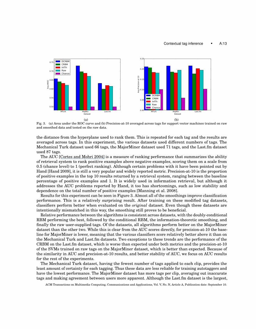
(a) (b)Fig. 3. (a) Area under the ROC curve and (b) Precision-at-10 averaged across tags for support vector machines trained on rawand smoothed data and tested on the raw data.

the distance from the hyperplane used to rank them. This is repeated for each tag and the results areaveraged across tags. In this experiment, the various datasets used different numbers of tags. TheMechanical Turk dataset used 66 tags, the MajorMiner dataset used 71 tags, and the Last.fm datasetused 87 tags.

The AUC [Cortes and Mohri 2004] is a measure of ranking performance that summarizes the abilityof retrieval system to rank positive examples above negative examples, scoring them on a scale from0.5 (chance level) to 1 (perfect ranking). Although certain problems with it have been pointed out byHand [Hand 2009], it is still a very popular and widely reported metric. Precision-at-10 is the proportionof positive examples in the top 10 results returned by a retrieval system, ranging between the baselinepercentage of positive examples and 1. It is widely used in information retrieval, but although itaddresses the AUC problems reported by Hand, it too has shortcomings, such as low stability anddependence on the total number of positive examples [Manning et al. 2008].

Results for this experiment can be seen in Figure 3. Almost all of the smoothings improve classificationperformance. This is a relatively surprising result. After training on these modified tag datasets,classifiers perform better when evaluated on the original dataset. Even though these datasets areintentionally mismatched in this way, the smoothing still proves to be beneficial.

Relative performance between the algorithms is consistent across datasets, with the doubly-conditionalRBM performing the best, followed by the conditional RBM, the information-theoretic smoothing, andfinally the raw user-supplied tags. Of the datasets, all algorithms perform better on the MajorMinerdataset than the other two. While this is clear from the AUC scores directly, for precision-at-10 the base-line for MajorMiner is lower, meaning that the various classifiers score relatively better above it than onthe Mechanical Turk and Last.fm datasets. Two exceptions to these trends are the performance of theCRBM on the Last.fm dataset, which is worse than expected under both metrics and the precision-at-10of the SVMs trained on raw tags on the MajorMiner dataset, which is better than expected. Because ofthe similarity in AUC and precision-at-10 results, and better stability of AUC, we focus on AUC resultsfor the rest of the experiments.

The Mechanical Turk dataset, having the fewest number of tags applied to each clip, provides theleast amount of certainty for each tagging. Thus these data are less reliable for training autotaggers andhave the lowest performance. The MajorMiner dataset has more tags per clip, averaging out inaccuratetags and making agreement between users more apparent. Although the Last.fm dataset is the largest,

ACM Transactions on Multimedia Computing, Communications and Applications, Vol. V, No. N, Article A, Publication date: September 10.

A:14 • Michael Mandel et al.

0.3 0.4 0.5 0.6 0.7 0.8 0.9gooddarkpop

happyvocals

smooth80sjazz

percussionclassicrock

femalebass

malevocalsalternative

upbeatlove

maleindie

ambientfun

pianoenergetic

classicfast

femalevocalscalmsoft

countryslowrockloud

guitarangryfunk

instrumentalsynthesizer

sadelectricguitar

bluesparty

technoclub

electronicafolkrap

hiphopdisco

danceacousticguitar

acoustic

DCRBMCRBMInfThRawChance

0.4 0.5 0.6 0.7 0.8 0.9 1.0organ

keyboardbass

voicedrum

80ssynth

solonoisevocal

trumpetrepetitive

popalternative

acousticbritishguitar

funkindie

femalestrings

electronicdrummachine

maleambient

endsaxophone

pianofast

electronicaslow

countrypunkclubbeatfolksoftrockjazz

dancetrancehouse

technometalballad

loudquiet

hiphoprap

silence

DCRBMCRBMInfThRawChance

0.40 0.45 0.50 0.55 0.60 0.65 0.70 0.75 0.80uk

britishfavouritefavorites

awesomeprogressiverock

90ssexy

guitarbritpop

postpunkexperimental

americanindierock

indiealternative

seenlive00sepic

newwaverockpop

alternativerockhardrock

psychedelic80s

melancholicpunk

electronicaelectronic

grungeheavymetalmelancholy

chillmetal

70striphop

beautifulalternativemetal

pianodowntempo

sadsingersongwriter

dancechillout

folkambient

60sacousticmellow

DCRBMCRBMInfThRawChance

(a) Mechanical Turk (b) MajorMiner (c) Last.fm

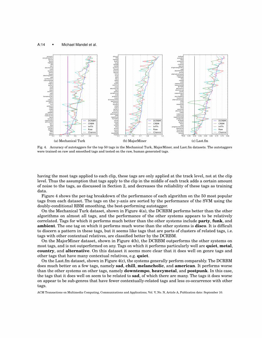
Fig. 4. Accuracy of autotaggers for the top 50 tags in the Mechanical Turk, MajorMiner, and Last.fm datasets. The autotaggerswere trained on raw and smoothed tags and tested on the raw, human generated tags.

having the most tags applied to each clip, these tags are only applied at the track level, not at the cliplevel. Thus the assumption that tags apply to the clip in the middle of each track adds a certain amountof noise to the tags, as discussed in Section 2, and decreases the reliability of these tags as trainingdata.

Figure 4 shows the per-tag breakdown of the performance of each algorithm on the 50 most populartags from each dataset. The tags on the y-axis are sorted by the performance of the SVM using thedoubly-conditional RBM smoothing, the best-performing autotagger.

On the Mechanical Turk dataset, shown in Figure 4(a), the DCRBM performs better than the otheralgorithms on almost all tags, and the performance of the other systems appears to be relativelycorrelated. Tags for which it performs much better than the other systems include party, funk, andambient. The one tag on which it performs much worse than the other systems is disco. It is difficultto discern a pattern in these tags, but it seems like tags that are parts of clusters of related tags, i.e.tags with other contextual relatives, are classified better by the DCRBM.

On the MajorMiner dataset, shown in Figure 4(b), the DCRBM outperforms the other systems onmost tags, and is not outperformed on any. Tags on which it performs particularly well are quiet, metal,country, and alternative. On this dataset it seems more clear that it does well on genre tags andother tags that have many contextual relatives, e.g. quiet.

On the Last.fm dataset, shown in Figure 4(c), the systems generally perform comparably. The DCRBMdoes much better on a few tags, namely sad, chill, melancholic, and american. It performs worsethan the other systems on other tags, namely downtempo, heavymetal, and postpunk. In this case,the tags that it does well on seem to be related to sad, of which there are many. The tags it does worseon appear to be sub-genres that have fewer contextually-related tags and less co-occurrence with othertags.ACM Transactions on Multimedia Computing, Communications and Applications, Vol. V, No. N, Article A, Publication date: September 10.

Contextual tag inference • A:15

0.3 0.4 0.5 0.6 0.7 0.8 0.9darkpop

happyvocals

smooth80sjazz

percussionclassicrock

femalebass

malevocalsalternative

upbeatlove

maleindie

ambientfun

pianorelaxed

energeticclassic

fastfemalevocals

calmsoft

countryslowrockloud

guitarangryfunk

instrumentalsynthesizer

sadelectricguitar

bluesparty

technoclub

electronicafolkrap

hiphopdisco

danceacousticguitar

acoustic

DCRBMCLPMLkNNRAkEL

0.3 0.4 0.5 0.6 0.7 0.8 0.9 1.0organ

keyboardbass

voicedrum

80ssynth

solonoisevocal

trumpetrepetitive

popalternative

acousticharmony

britishindustrial

guitarfunkindie

femalestrings

electronicmale

ambientend

saxophonepiano

fastelectronica

slowcountry

punkclubbeatfolksoftrockjazz

dancetrancehouse

technometalballad

loudquiet

rapsilence

DCRBMCLPMLkNNRAkEL

MTurk MajMinDataset

0.50

0.55

0.60

0.65

0.70

0.75

Avg A

RO

C

DCRBMCLPMLkNNRAkEL

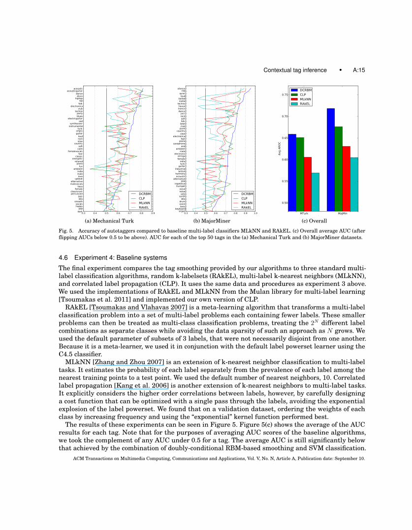
(a) Mechanical Turk (b) MajorMiner (c) Overall

Fig. 5. Accuracy of autotaggers compared to baseline multi-label classifiers MLkNN and RAkEL. (c) Overall average AUC (afterflipping AUCs below 0.5 to be above). AUC for each of the top 50 tags in the (a) Mechanical Turk and (b) MajorMiner datasets.

4.6 Experiment 4: Baseline systems

The final experiment compares the tag smoothing provided by our algorithms to three standard multi-label classification algorithms, random k-labelsets (RAkEL), multi-label k-nearest neighbors (MLkNN),and correlated label propagation (CLP). It uses the same data and procedures as experiment 3 above.We used the implementations of RAkEL and MLkNN from the Mulan library for multi-label learning[Tsoumakas et al. 2011] and implemented our own version of CLP.

RAkEL [Tsoumakas and Vlahavas 2007] is a meta-learning algorithm that transforms a multi-labelclassification problem into a set of multi-label problems each containing fewer labels. These smallerproblems can then be treated as multi-class classification problems, treating the 2N different labelcombinations as separate classes while avoiding the data sparsity of such an approach as N grows. Weused the default parameter of subsets of 3 labels, that were not necessarily disjoint from one another.Because it is a meta-learner, we used it in conjunction with the default label powerset learner using theC4.5 classifier.

MLkNN [Zhang and Zhou 2007] is an extension of k-nearest neighbor classification to multi-labeltasks. It estimates the probability of each label separately from the prevalence of each label among thenearest training points to a test point. We used the default number of nearest neighbors, 10. Correlatedlabel propagation [Kang et al. 2006] is another extension of k-nearest neighbors to multi-label tasks.It explicitly considers the higher order correlations between labels, however, by carefully designinga cost function that can be optimized with a single pass through the labels, avoiding the exponentialexplosion of the label powerset. We found that on a validation dataset, ordering the weights of eachclass by increasing frequency and using the “exponential” kernel function performed best.

The results of these experiments can be seen in Figure 5. Figure 5(c) shows the average of the AUCresults for each tag. Note that for the purposes of averaging AUC scores of the baseline algorithms,we took the complement of any AUC under 0.5 for a tag. The average AUC is still significantly belowthat achieved by the combination of doubly-conditional RBM-based smoothing and SVM classification.

ACM Transactions on Multimedia Computing, Communications and Applications, Vol. V, No. N, Article A, Publication date: September 10.

A:16 • Michael Mandel et al.

The AUC for each of the top 50 tags can be seen in Figure 5(a) and (b) for the Mechanical Turk andMajorMiner datasets, respectively. On the Mechanical Turk dataset, the DCRBM achieved a higherAUC for a large majority of the tags except for the notable exceptions of disco, electronica, classical,and energetic. On the MajorMiner dataset, the DCRBM performed better than the baseline algorithmson all tags except for small differences on saxophone, ambient, repetitive, and electronic. Thisevidence solidly supports the conclusion that DCRBM is able to out-perform other multi-label classifierson these tasks.

5. CONCLUSIONS

These experiments show that the autotagging of music becomes more accurate when augmented withcontextual information, both in terms of tag co-occurrence context and temporal context. Temporalcontext can be employed because of the higher correlations shown to exist between the tags applied toclips that are “closer” to one another temporally. Tag-tag context can be applied because of synonymyand other contextual relationships between tags. These results are an important step in developingmusic classification and categorization beyond a series of isolated tag problems and clip examples to amore holistic approach that considers music and tags in their rich contextual relationships.

In addition to these ideas about context, this paper has contributed two new realizations of contextualtag language models in the form of conditional restricted Boltzmann machines. These models achievebetter AUC performance than other state-of-the-art multi-label classifiers on this problem. It has alsoshown the value for capturing tag-tag context of information theoretic models that have previously beenshown to accurately predict friendship links in social networks. Both of these modeling strategies couldbe applied to images, video, or many other modalities in which social tags are useful, but frequentlysparse.

In the future, we would like to extend this work by modeling audio and tags jointly, instead ofrequiring separate tag-smoothing and classifier training stages. One candidate for such a model is thediscriminative RBM [Larochelle and Bengio 2008; Mandel et al. 2011], which is closely related to theconditional RBMs employed in this paper. We would also like to exploit unlabeled and weakly labeleddata, for example large collections of unlabeled music and large collections of text about music. RBMsand particularly discriminative RBMs look quite promising for such tasks. Finally, we would like toexpand our use of information theoretic models beyond the tag-tag similarity to take advantage of thefurther context and richness available in the full set of (user, item, tag) triples.

ACKNOWLEDGMENTS

We are grateful to Last.fm for making their data available. This work was partly supported by theproject Social Integration of Semantic Annotation Networks for Web Applications funded by NationalScience Foundation award IIS-0811994.

REFERENCES

AUCOUTURIER, J., PACHET, F., ROY, P., AND BEURIV, A. 2007. Signal + context = better classification. In Proc. ISMIR. 425–430.BERTIN-MAHIEUX, T., ECK, D., MAILLET, F., AND LAMERE, P. 2008. Autotagger: A model for predicting social tags from acoustic

features on large music databases. J. New Music Res. 37, 2, 115—135.BESAG, J. 1975. Statistical analysis of non-lattice data. The Statistician 24, 3, 179–195.BOUTELL, M., LUO, J., SHEN, X., AND BROWN, C. 2004. Learning multi-label scene classification1. Pattern Recognition 37, 9,

1757–1771.CHEN, L., XU, D., TSANG, I. W., AND LUO, J. 2010. Tag-based web photo retrieval improved by batch mode re-tagging. 3440–3446.CORTES, C. AND MOHRI, M. 2004. Auc optimization vs. error rate minimization. In NIPS 16, S. Thrun, L. Saul, and B. Scholkopf,

Eds. Vol. 16. MIT Press, Cambridge, MA.

ACM Transactions on Multimedia Computing, Communications and Applications, Vol. V, No. N, Article A, Publication date: September 10.

Contextual tag inference • A:17

ECK, D., LAMERE, P., BERTIN-MAHIEUX, T., AND GREEN, S. 2008. Automatic generation of social tags for music recommendation.In NIPS 20, J. Platt, D. Koller, Y. Singer, and S. Roweis, Eds. MIT Press, Cambridge, MA, 385–392.

HAN, Y., WU, F., JIA, J., ZHUANG, Y., AND YU, B. 2010. Multi-task sparse discriminant analysis (mtsda) with overlappingcategories. In AAAI Conference on Artificial Intelligence. 469–474.

HAND, D. J. 2009. Measuring classifier performance: a coherent alternative to the area under the ROC curve. Mach. Learn. 77,103–123.

HEITZ, G. AND KOLLER, D. 2008. Learning spatial context: Using stuff to find things. In ECCV, D. Forsyth, P. Torr, andA. Zisserman, Eds. Lecture Notes in Computer Science Series, vol. 4. Springer Berlin / Heidelberg, Berlin, Heidelberg, 30–43.

HINTON, G. 2002. Training products of experts by minimizing contrastive divergence. Neural Computation 14, 1771–1800.HOIEM, D., EFROS, A., AND HEBERT, M. 2008. Putting objects in perspective. International Journal of Computer Vision 80, 1,

3–15.KANG, F., JIN, R., AND SUKTHANKAR, R. 2006. Correlated Label Propagation with Application to Multi-label Learning. In Intl.

Conf. on Comp. Vision and Pat. Rec. 1719–1726.LAROCHELLE, H. AND BENGIO, Y. 2008. Classification using discriminative restricted Boltzmann machines. In Proc. ICML,

A. McCallum and S. Roweis, Eds. Omnipress, 536–543.LEE, J. H. 2010. Crowdsourcing music similarity judgments using mechanical turk. In Proc. ISMIR. 183–188.MANDEL, M., PASCANU, R., LAROCHELLE, H., AND BENGIO, Y. 2011. Autotagging music with conditional restricted boltzmann

machines. Online: http://arxiv.org/abs/1103.2832.MANDEL, M. I., ECK, D., AND BENGIO, Y. 2010. Learning tags that vary within a song. In Proc. ISMIR. 399–404.MANDEL, M. I. AND ELLIS, D. P. W. 2008. A web-based game for collecting music metadata. J. New Music Res. 37, 2, 151–165.MANNING, C., RAGHAVAN, P., AND SCHUTZE, H. 2008. Introduction to information retrieval. Cambridge University Press.MARKINES, B., CATTUTO, C., MENCZER, F., BENZ, D., HOTHO, A., AND STUMME, G. 2009. Evaluating similarity measures for

emergent semantics of social tagging. In Proceedings of the 18th international conference on World wide web. ACM, 641–650.MIOTTO, R., BARRINGTON, L., AND LANCKRIET, G. 2010. Improving auto-tagging by modeling semantic co-occurrences. In Proc.

ISMIR. 297–302.MURPHY, K., TORRALBA, A., AND FREEMAN, W. T. 2004. Using the forest to see the trees: A graphical model relating features,

objects, and scenes. In NIPS 16, S. Thrun, L. Saul, and B. Scholkopf, Eds. MIT Press, Cambridge, MA.RABINOVICH, A., VEDALDI, A., GALLEGUILLOS, C., WIEWIORA, E., AND BELONGIE, S. 2007. Objects in context. In Intl. Conf.

on Computer Vision. IEEE, 1–8.RASIWASIA, N. AND VASCONCELOS, N. 2009. Holistic context modeling using semantic co-occurrences. In Intl. Conf. on Comp.

Vision and Pat. Rec. IEEE, Los Alamitos, CA, USA, 1889–1895.SALAKHUTDINOV, R., MNIH, A., AND HINTON, G. 2007. Restricted Boltzmann machines for collaborative filtering. In Proc.

ICML. 791–798.SCHIFANELLA, R., BARRAT, A., CATTUTO, C., MARKINES, B., AND MENCZER, F. 2010. Folks in folksonomies: Social link

prediction from shared metadata. In Proc. ACM Intl. Conf. on Web search and data mining. ACM, 271–280.SLANEY, M. 2002. Semantic-audio retrieval. In Proc. ICASSP. Vol. 4.SMOLENSKY, P. 1986. Information processing in dynamical systems: foundations of harmony theory. MIT Press.SNOW, R., O’CONNOR, B., JURAFSKY, D., AND NG, A. 2008. Cheap and fast – but is it good? evaluating non-expert annotations

for natural language tasks. In Proc. Empirical Methods in NLP. 254–263.SOROKIN, A. AND FORSYTH, D. 2008. Utility data annotation with amazon mechanical turk. In CVPR Workshops. 1–8.TAYLOR, G., HINTON, G. E., AND ROWEIS, S. 2007. Modeling human motion using binary latent variables. In NIPS 19,

B. Scholkopf, J. Platt, and T. Hoffman, Eds. MIT Press, Cambridge, MA, 1345–1352.TINGLE, D., KIM, Y. E., AND TURNBULL, D. 2010. Exploring automatic music annotation with “acoustically-objective” tags. In

Proc. Intl. Conf. on Multimedia inf. retr. ACM, 55–62.TROHIDIS, K., TSOUMAKAS, G., KALLIRIS, G., AND VLAHAVAS, I. 2008. Multilabel classification of music into emotions. In Proc.

ISMIR.TSOUMAKAS, G., KATAKIS, I., AND VLAHAVAS, I. 2010. Mining multi-label data. In Data Mining and Knowledge Discovery

Handbook, O. Maimon and L. Rokach, Eds. Chapter 34, 667–685.TSOUMAKAS, G., VILCEK, J., SPYROMITROS, L., AND VLAHAVAS, I. 2011. MULAN: a java library for multi-label learning.

Journal of Machine Learning Research. Accepted for publication conditioned on minor revisions.TSOUMAKAS, G. AND VLAHAVAS, I. 2007. Random k-Labelsets: An ensemble method for multilabel classification. In Proc. ECML.

Lecture Notes in Computer Science Series, vol. 4701. Springer Berlin / Heidelberg, Berlin, Heidelberg, Chapter 38, 406–417.

ACM Transactions on Multimedia Computing, Communications and Applications, Vol. V, No. N, Article A, Publication date: September 10.

A:18 • Michael Mandel et al.

WHITEHILL, J., RUVOLO, P., WU, T., BERGSMA, J., AND MOVELLAN, J. 2009. Whose vote should count more: Optimal integrationof labels from labelers of unknown expertise. In NIPS 22, Y. Bengio, D. Schuurmans, C. Williams, J. Lafferty, and A. Culotta,Eds. 2035–2043.

WHITMAN, B. AND RIFKIN, R. 2002. Musical query-by-description as a multiclass learning problem. In IEEE Workshop onMultimedia Signal Processing. 153–156.

YAO, B. AND FEI-FEI, L. 2010. Modeling mutual context of object and human pose in human-object interaction activities. In Intl.Conf. on Comp. Vision and Pat. Rec. IEEE, 17–24.

ZHANG, M. AND ZHOU, Z. 2007. ML-KNN: A lazy learning approach to multi-label learning. Pattern Recognition 40, 7, 2038–2048.

Received September 2010; revised March 2011; accepted August 2011

ACM Transactions on Multimedia Computing, Communications and Applications, Vol. V, No. N, Article A, Publication date: September 10.