Embed Size (px)
Citation preview

Journal of Graph Algorithms and Applicationshttp://jgaa.info/ vol. 10, no. 1, pp. 5–49 (2006)
Contraction and Treewidth Lower Bounds
Hans L. Bodlaender Thomas Wolle
Institute of Information and Computing Sciences, Utrecht UniversityP.O. Box 80.089, 3508 TB Utrecht, The Netherlands
http://www.cs.uu.nl/[email protected] [email protected]
Arie M. C. A. Koster
Zuse Institute Berlin (ZIB)Takustraße 7, D-14194 Berlin, Germany
http://www.zib.de/[email protected]
Abstract
Edge contraction is shown to be a useful mechanism to improve lowerbound heuristics for treewidth. A successful lower bound for treewidthis the degeneracy: the maximum over all subgraphs of the minimum de-gree. The degeneracy is polynomial time computable. We introduce thenotion of contraction degeneracy: the maximum over all minors of theminimum degree. We show that the contraction degeneracy problem isNP-complete, even for bipartite graphs, but for fixed k, it is polynomialtime decidable if a given graph G has contraction degeneracy at leastk. Heuristics for computing the contraction degeneracy are proposed andevaluated. It is shown that these can lead in practice to considerableimprovements of the lower bound for treewidth, but can perform arbi-trarily bad on some examples. A study is also made for the combinationof contraction with Lucena’s lower bound based on Maximum CardinalitySearch [27]. Finally, heuristics for the treewidth are proposed and eval-uated that combine contraction with a treewidth lower bound techniqueby Clautiaux et al. [12].
Article Type Communicated by Submitted Revised
regular paper Tomasz Radzik August 2004 July 2005
This work was partially supported by the DFG research group “Algorithms, Structure,
Randomness” (Grant GR 883/9-3, GR 883/9-4), and by the Netherlands Organisation
for Scientific Research NWO (project Treewidth and Combinatorial Optimisation).

H. L. Bodlaender et al., Contraction and Treewidth, JGAA, 10(1) 5–49 (2006)6
1 Introduction
It is about two decades ago that the notion of treewidth and the equivalentnotion of partial k-tree were introduced. Nowadays, these play an importantrole in many theoretic studies in graph theory and algorithms, but also their usefor practical applications is growing, see e.g. [23, 25]. A first step when solvingproblems on graphs of bounded treewidth is to compute a tree decompositionof (close to) optimal width, on which often a dynamic programming approach isapplied. Such a dynamic programming algorithm typically has a running timethat is exponential in the treewidth of the graph. Since the treewidth problem isNP-complete [1], it is rather unlikely to find efficient algorithms for computingthe treewidth. Therefore, we are interested in lower and upper bounds for thetreewidth of a graph.
This paper focuses on lower bounds on the treewidth of a graph. Goodlower bounds can serve to speed up branch and bound methods, inform usabout the quality of upper bound heuristics, and in some cases, tell us that weshould not use tree decompositions to solve a problem on a certain instance.A large lower bound on the treewidth of a graph implies that we should nothope for computationally efficient dynamic programming algorithms that usetree decompositions for this particular instance.
More work has been done recently on practical algorithms for determiningthe treewidth of graphs, for instance on preprocessing methods (see [8, 9, 18]),upper bound heuristics (e.g. [12, 13, 20, 22]), lower bound heuristics (e.g. [7, 12,27, 29]), and some exact methods (e.g. [20, 33]). In many cases, exact methodsare still too slow, and for many instances, there are large gaps between thebounds given by upper bound and lower bound heuristics. Thus, the study ofalgorithms and heuristics for treewidth remains interesting also from a practicalpoint of view.
In this paper, we propose and study algorithms that find lower bounds fortreewidth using contraction of edges. In each of the algorithms, we have acombination of contraction with existing lower bound methods. In particular, westudy how contraction can be used to improve the degeneracy (or MMD) lowerbound [22], the lower bound based on maximum cardinality search MCSLB,introduced by Lucena [27], and the technique introduced by Clautiaux et al. [12].Descriptions of these existing lower bound methods can be found in Section 2.
Contraction of an edge is the operation that replaces its two endpoints by asingle vertex, which is adjacent to all vertices at least one of the two endpointswas adjacent to. Combining the notion of contraction with degeneracy givesthe new notion of contraction degeneracy of a graph G: the maximum of theminimum degree over all graphs that can be obtained by contracting edges andtaking subgraphs of G. It provides us with a new lower bound on the treewidthof graphs. While unfortunately, computing the contraction degeneracy of agraph is NP-complete (as is shown in Section 3.2), the fixed parameter casesare polynomial time solvable (see Section 3.3), and there are simple heuristicsthat provide us with good bounds on several instances taken from real lifeapplications (see Section 5).

H. L. Bodlaender et al., Contraction and Treewidth, JGAA, 10(1) 5–49 (2006)7
In a very recent paper, Gogate and Dechter [20] propose a branch and boundalgorithm for treewidth with a good anytime performance. Independently ofour work, Gogate and Dechter also propose the lower bound heuristic whichwe call the MMD+(min-d) heuristic in this paper. We compare this heuristicwith other heuristics in Section 6, and see that the strategy where we contractto a neighbour with minimum number of common neighbours almost alwaysoutperforms the MMD+(min-d) heuristic where we contract to a neighbour ofminimum degree. For more details, see [20], Section 3 and Section 6.
The lower bound provided by MCSLB is never smaller than the degeneracy,but can be larger [7]. This motivates the study of contraction in combinationwith the MCSLB algorithm. Combining MCSLB with contraction was first usedby Lucena in [26]. Unfortunately, the problem to determine if some bound canbe obtained with MCSLB for a graph obtained from G by contracting edges isalso NP-complete (Section 4.2). Its fixed parameter case is linear time solvable(Section 4.3). We also studied some heuristics for this bound.
In our experiments, we have seen that, typically, the bound by MCSLB isequal to the degeneracy or slightly larger. In both cases, often a large increasein the lower bound is obtained when we combine the method with contraction.See Section 6 for results of our computational experiments. They show thatcontraction is a very viable idea for obtaining or improving treewidth lowerbounds.
A further improvement to the lower bounds can be obtained by using amethod found by Clautiaux et al. [12]. This method uses another treewidthlower bound algorithm as a subroutine. In [12], the authors use the degeneracy(or MMD) as a subroutine, but one can also use other algorithms. Our exper-iments showed that the contraction degeneracy heuristics generally outperformthe method of [12] with degeneracy, but when we combine the method of [12]with the heuristics of this paper, we get in several cases an additional smallimprovement to the lower bound. We finally propose a heuristic that combinesthe method of [12] and contraction in another way, by doing a contraction be-tween every round of ‘graph improvement’. See Section 5 for more details. Thislatter heuristic often costs considerably more time, but can give also significantincreases to the lower bound.
2 Preliminaries
Throughout the paper G = (V,E) denotes a simple undirected graph. Mostof our terminology is standard graph theory/algorithm terminology. n denotesthe number of vertices of the input graph G = (V,E). As usual, the degreein G of vertex v is dG(v) or simply d(v). N(S) for S ⊆ V denotes the openneighbourhood of S, i.e. N(S) =
⋃s∈S N(s) \ S. A vertex v ∈ V is universal in
a graph G = (V,E), if v is adjacent to all other vertices. We define:
δ(G) := minv∈V
d(v)

H. L. Bodlaender et al., Contraction and Treewidth, JGAA, 10(1) 5–49 (2006)8
Subgraphs and Minors. After deleting vertices of a graph and their incidentedges, we get an induced subgraph. For a graph G = (V,E) and set of verticesW ⊆ V , the subgraph of G induced by W is denoted G[W ] = (W, v, w ∈E | v, w ∈ W). A subgraph is obtained, if we additionally allow deletion ofedges. If we furthermore allow edge-contractions, we get a minor. It is knownthat the treewidth of a minor of G is at most the treewidth of G (see e.g. [4]).We explicitly exclude the null graph (the graph without vertices and withoutedges) as a minor or subgraph.
Edge-Contraction. Contracting edge e = u, v in the graph G = (V,E),denoted as G/e, is the operation that introduces a new vertex ae and newedges, such that ae is adjacent to all the neighbours of v and u, and deletesvertices u and v and all edges incident to u or v:
G/e := (V ′, E′), where
V ′ = ae ∪ V \ u, vE′ = ae, x | x ∈ N(u, v) ∪ E \ e′ ∈ E | e′ ∩ e 6= ∅
A contraction-set is a cycle free set E′ ⊆ E(G) of edges. Note that after each sin-gle edge-contraction the names of the vertices are updated in the graph. Hence,for two adjacent edges e = u, v and f = v, w, edge f will be differentafter contracting edge e, namely in G/e we have f = ae, w. Still, for conve-nience, we let f represent the same edge in G and in G/e. For a contraction-setE′ = e1, e2, . . . , ep, we define G/E′ := G/e1/e2/ . . . /ep. Furthermore, notethat the order of edge-contractions to obtain G/E′ is not relevant. A contractionH of G is a graph such that there exists a contraction-set E′ with: H = G/E′.
A graph H = (VH , EH) is a subdivision of a graph G = (V,E), if H can beobtained from G by zero or more subdivision operations; a subdivision operationreplaces an edge v, w by a new vertex x and two edges v, x and x,w.
Treewidth. A tree decomposition of G = (V,E) is a pair (Xi | i ∈ I, T =(I, F )), with Xi | i ∈ I a family of subsets of V , and T a tree, such that
• ⋃i∈I Xi = V .
• For all v, w ∈ E, there is an i ∈ I with v, w ∈ Xi.
• For all i0, i1, i2 ∈ I: if i1 is on the path from i0 to i2 in T , then Xi0 ∩Xi2 ⊆Xi1 .
The width of tree decomposition (Xi | i ∈ I, T = (I, F )) is maxi∈I |Xi| − 1.The treewidth tw(G) of G is the minimum width among all tree decompositionsof G.
One can alternatively define the treewidth in terms of chordal graphs. Agraph is chordal, if and only if it does not contain an induced cycle with lengthat least four. The treewidth of a graph is exactly the minimum over all chordalgraphs H that contain G as a subgraph of the size of the maximum clique in Hminus 1, see [4].

H. L. Bodlaender et al., Contraction and Treewidth, JGAA, 10(1) 5–49 (2006)9
Degeneracy/MMD. We also use the term MMD (Maximum Minimum De-gree) for the degeneracy. The degeneracy δD of a graph G is defined to be:
δD(G) := maxG′
δ(G′) | G′ is a subgraph of G
The minimum degree of a graph is a lower bound on its treewidth, and thetreewidth of G cannot increase by taking subgraphs. Hence, the treewidth of Gis at least its degeneracy. (See also [22].)
Maximum Cardinality Search. MCS is a method to number the vertices ofa graph. It was first introduced by Tarjan and Yannakakis for the recognitionof chordal graphs [34]. We start by giving some vertex number 1. In stepi = 2, . . . , n, we choose an unnumbered vertex v that has the largest numberof already numbered neighbours, breaking ties as we wish. Then we associatenumber i to vertex v. An MCS ordering ψ can be defined by mapping eachvertex to its number: ψ(v) := number of v. For a fixed MCS ordering, letvi := ψ−1(i).
Definition 1 Let be given a graph G and an MCS ordering ψ of G, and letvi := ψ−1(i). The visited degree vdψ(vi) of vi is defined as follows:
vdψ(vi) := dG[v1,...,vi](vi)
The visited degree MCSLBψ of an MCS ordering ψ is defined as follows:
MCSLBψ := maxi=1,...,n
vdψ(vi)
In [27], Lucena shows that for every graph G and MCS ordering ψ of G,
MCSLBψ ≤ tw(G)
Thus, an MCS numbering gives a lower bound on the treewidth of a graph.In [7], it was shown that it is NP-hard to compute the maximum over all
MCS orderings ψ of MCSLBψ; more precisely, deciding if maxMCSLBψ | ψis an MCS ordering of G ≥ 7 is NP-complete.
Improved Graphs. In [5], two notions of improved graphs were introduced.Let k be an integer. The (k + 1)-neighbours improved graph G′ = (V,E′) ofG = (V,E) is obtained as follows: we take G, and then, as long as there arenon-adjacent vertices u, v, that have at least k + 1 common neighbours in thegraph, we add the edge u, v. This improvement step is motivated by thefollowing lemma.
Lemma 1 (See [3, 5, 12].) Any tree decomposition of G with width at mostk is also a tree decomposition of the (k+ 1)-neighbours improved graph G′ of Gwith width at most k, and vice versa.
H. L. Bodlaender et al., Contraction and Treewidth, JGAA, 10(1) 5–49 (2006)10
Clautiaux et al. use improved graphs to provide iterative methods to improveexisting lower bounds for treewidth [12]. They use the MMD for computinglower bounds, but their approach works with every lower bound heuristic. Theiralgorithm LB N works as follows:
• Suppose we have a lower bound LB ≤ tw(G) on the treewidth of G (e.g.LB was computed with the MMD heuristic).
• Use as hypothesis that LB = tw(G). Build the (LB + 1)-neighboursimproved graph G′ of G. (Note that if the hypothesis holds, then tw(G) =tw(G′))
• Compute a lower bound LB′ of G′ (e.g. with the MMD heuristic).
• If LB′ > LB, we have a contradiction, showing the hypothesis LB =tw(G) to be wrong.
• Therefore, LB < tw(G) and LB + 1 is also a lower bound.
• Set LB to LB + 1, and repeat the process until there is no contradiction.
We see that the LB N algorithm uses another treewidth lower bound algo-rithm as a subroutine, and thus, for every choice of such an algorithm, we obtaina different version of the LB N algorithm. If algorithm Y is used as subroutine,then we call the resulting algorithm LBN(Y), e.g. the algorithm discussed byClautiaux et al. in [12] is the LBN(MMD) algorithm.
In [12], Clautiaux et al. also propose a related method, that sometimes givesbetter lower bounds, but also uses more time. Here, we have a different notionof improved graph. Let k be an integer. The (k + 1)-paths improved graphG′′ = (V,E′′) of G = (V,E) is obtained by adding an edge u, v to E for allvertex pairs u and v such that there are at least k + 1 vertex disjoint pathsbetween u and v in G. Similar to Lemma 1, we have here the following.
Lemma 2 (See [3, 5, 12].) Any tree decomposition of G with width at mostk is also a tree decomposition of the (k+ 1)-paths improved graph G′′ of G withwidth at most k, and vice versa.
We can build the (k + 1)-paths improved graph in polynomial time, as we candecide in polynomial time whether there are at least k+ 1 vertex disjoint pathsbetween a pair of vertices with help of network flow techniques. However, therunning time to compute the paths improved graph is much larger than for theneighbour version. If we use (k + 1)-paths improved graphs instead of (k + 1)-neighbours improved graphs, then we obtain a new lower bound heuristic fortreewidth, called LB P in [12]. If we use as subroutine a lower bound algorithmY in this algorithm, we call the resulting algorithm LBP(Y).

H. L. Bodlaender et al., Contraction and Treewidth, JGAA, 10(1) 5–49 (2006)11
3 Contraction Degeneracy
We first look at the treewidth lower bound heuristic, obtained by combiningthe degeneracy with contraction. The algorithm to compute the degeneracyof a graph repeatedly removes the vertex of minimum degree, and outputs thelargest of these minimum degrees seen in the process. However, we can also geta lower bound for treewidth if we contract the vertex of minimum degree witha neighbour instead of deleting it. In this case, we can get different values if wemake different choices which minimum degree vertex to select, and with whichneighbour to contract it. The best way of doing these contractions is capturedby the notion of contraction degeneracy.
In this section, we define the new parameter of contraction degeneracy andthe related computational problem. We show the NP-completeness of the prob-lem just defined, and consider the complexity of the fixed parameter cases.
3.1 Definition of the Problem
Definition 2 The contraction degeneracy δC of a graph G is defined as follows:
δC(G) := maxG′
δ(G′) | G′ is a minor of G
When G is connected, δC(G) can also be defined as the maximum over allcontractions of G of the minimum degree of the contraction. This does notnecessarily hold for disconnected graphs: when G has connected componentswhose contraction degeneracy is smaller than the contraction degeneracy of G,we must delete this component entirely to obtain the minor with maximumminimum degree. The corresponding decision problem is formulated as usual:
Problem: Contraction Degeneracy
Instance: Graph G = (V,E) and integer k ≥ 0.Question: Is the contraction degeneracy of G at least k?
Lemma 3 For any graph G, we have that δC(G) ≤ tw(G).
Proof: Note that for any minor G′ of G, we have that tw(G′) ≤ tw(G) (seee.g. [4]). Furthermore, for any graph G′: δ(G′) ≤ tw(G′). The lemma followsnow directly. 2
3.2 NP-completeness
Theorem 1 The Contraction Degeneracy problem is NP-complete.
Proof: Clearly, the problem is in NP as we only have to guess an edge set E′,and then compute in polynomial time δ(G/E′).
The hardness proof is a transformation from the Vertex Cover problem,which is known to be NP-complete, see [19]. In the Vertex Cover problem,we are given a graph G = (V,E) and an integer k, and look for a vertex cover of

H. L. Bodlaender et al., Contraction and Treewidth, JGAA, 10(1) 5–49 (2006)12
w1
uk
Gu
u1
w2
2
Figure 1: Graph G′ constructed for the transformation.
size at most k, i.e. a set W ⊆ V with |W | ≤ k, such that each edge in E has atleast one endpoint in W . Let be given a Vertex Cover instance (G, k), withG = (V,E). Suppose k ≤ |V |.
Construction: We construct a graph G′ by taking the complement G of G,adding two adjacent vertices and k pairwise non-adjacent vertices, and makingthe new vertices adjacent to each vertex in G. G′ is formally defined as follows,see Figure 1:
G′ := (V ′, E′) where
V ′ = V ∪ w1, w2 ∪ u1, . . . , ukE′ = (v, w 6∈ E | v, w ∈ V, v 6= w) ∪ w1, w2
∪ wi, v | i ∈ 1, 2 ∧ v ∈ V ∪ ui, v | i ∈ 1, . . . , k ∧ v ∈ V
Let be n := |V |. The constructed instance of the Contraction Degener-
acy problem is (G′, n+ 1).Now, we have to show that there is a vertex cover for G of size at most k if,
and only if δC(G′) ≥ n+ 1.
Claim 1 If there is a vertex cover of G of size at most k, then there is aE1 ⊆ E′, such that δ(G′/E1) ≥ n+ 1.
Proof: Suppose there is a vertex cover of size at most k. Now take a vertexcover V1 = v1, . . . , vk of G of size exactly k. (If we add vertices to a vertexcover, we obtain again a vertex cover.) Let E1 = ui, vi | i = 1, . . . , k. I.e.,each vertex in the vertex cover has a vertex of the type ui contracted to it; wecan do this because each vertex ui is adjacent to every vertex of G in the graphG′. We claim that the graph obtained from G′ by contracting E1, G
′/E1 is an(n+ 2)-clique. Assume there are two vertices x and y with x, y 6∈ E(G′/E1).Since the vertices w1 and w2 are universal in G′/E1, we have x, y ⊆ V .Therefore, x, y is not an edge in G, hence x, y ∈ E, and thus x or y isin V1. We assume w.l.o.g. x ∈ V1, i.e. ∃i ∈ 1, . . . , k, such that vi = x.Since we contracted ui, vi and ui, y ∈ E(G′), we have vi = x is adjacent

H. L. Bodlaender et al., Contraction and Treewidth, JGAA, 10(1) 5–49 (2006)13
to y in G′/E1, which is a contradiction. Hence, G′/E1 is an (n+ 2)-clique andδ(G′/E1) = n+ 1. ⋄
Claim 2 If there is a E1 ⊆ E′, such that δ(G′/E1) ≥ n + 1, then there is avertex cover V1 for G of size at most k.
Proof: For all i ∈ 1, . . . , k, vertex ui has degree exactly n in G′. Thus,for each ui, i ∈ 1, . . . , k, we have to contract an edge incident to ui. Asthere are no edges ui, uj in G′, contracting the edges incident to verticesui, i ∈ 1, . . . , k removes k vertices from the graph. Thus, after contractingthese edges, there are n + 2 vertices left in the graph. Therefore we cannotcontract another edge, since then we could not obtain the minimum degree ofn+ 1. Furthermore, we see that G′/E1 is an (n+ 2)-clique. Hence, E1 containsexactly k edges, one for every ui, i ∈ 1, . . . , k, with the other endpoint in V .Let be V1 :=
⋃e∈E1
e \ ⋃i=1,...kui. Clearly, |V1| = k, and we claim that V1 is
a vertex cover of G. Assume, there is an edge f = x, y in G with V1 ∩ f = ∅.Hence, f is not an edge in G′. Since G′/E1 is an (n+2)-clique, edge f exists inG′/E1, which means: f was created by contracting another edge ui, vj ∈ E1.This can only be the case if vj = x or vj = y. According to the definition of V1,we have: vj ∈ V1, which contradicts V1 ∩ f = ∅. Hence, V1 is a vertex cover ofsize k. ⋄As G∗ can be constructed in polynomial time, NP-completeness of the Con-
traction Degeneracy problem now follows. 2
Lemma 4 If H is a subdivision of G, then δC(G) = δC(H).
Proof: We can use induction to the number of subdivision operations appliedto G in order to obtain H, and thus it is sufficient to show that δC(G) =δC(H) if H is obtained from G by one subdivision operation. Say edge v, wis subdivided, and replaced by vertex x and edges v, x and x,w.
δC(G) ≤ δC(H), as we obtain any contraction of G as contraction of H bystarting with contracting the edge v, x.
If δC(G) = 1, then G is a forest, hence H is a forest, and δC(H) = 1. IfδC(G) ≥ 2, then a contraction of H with minimum degree larger than δC(G) ≥2 cannot contain the degree-2 vertex x, so must include a contraction of avertex with x. By commutativity of contraction, we can assume that we startby contracting x with a neighbour, so any contraction of H with minimumdegree larger than δC(G) must be a contraction of a graph isomorphic to G.We conclude that no such contraction exists, and δC(G) = δC(H). 2
Corollary 1 The Contraction Degeneracy problem is NP-complete, evenfor bipartite graphs.
Proof: We transform from the Contraction Degeneracy problem on arbi-trary graphs. Given an instance (G, k) of Contraction Degeneracy, takethe instance (H, k) where H is obtained by subdividing each edge of G. H isbipartite, and by Lemma 4, the two instances are equivalent. 2

H. L. Bodlaender et al., Contraction and Treewidth, JGAA, 10(1) 5–49 (2006)14
3.3 Fixed Parameter Cases of Contraction Degeneracy
Now, we consider the fixed parameter case of the Contraction Degeneracy
problem. I.e. for a fixed integer k, we consider the problem to decide for agiven graph G if G has a minor with minimum degree k. Graph minor theorygives a fast answer to this problem. For a good introduction to the algorithmicconsequences of this theory, see [17].
Theorem 2 The Contraction Degeneracy problem can be solved in lineartime when k is a fixed integer with k ≤ 5, and can be solved in O(n3) time whenk is a fixed integer with k ≥ 6.
Proof: Let k be a fixed integer. Consider the class of graphs Gk = G | Ghas contraction degeneracy at most k − 1. Gk is closed under taking minors:if H is a minor of G and H has contraction degeneracy at least k, then Ghas also contraction degeneracy at least k. As every class of graphs that isclosed under minors has an O(n3) algorithm to test membership by Robertson-Seymour graph minor theory (see [17]), the theorem for the case that k ≥ 6follows.
Suppose now that k ≤ 5. There exists a planar graph Gk with minimumdegree k (for example for k = 5 the icosahedron, see [11]). Hence, Gk 6∈ Gk.A class of graphs that is closed under taking minors and does not contain allplanar graphs has a linear time membership test (see [17]), which shows theresult for the case that k ≤ 5. 2
It can be noted that the cases that k = 1, 2 and 3 are very simple: a graphhas contraction degeneracy at least 1, if and only if it has at least one edge,and it has contraction degeneracy at least 2, if and only if it is not a forest. Fora graph to have contraction degeneracy at least 3, all vertices of degree 2 orless have to be contracted recursively. If the result is a non-empty graph, thecontraction degeneracy is at least 3. Vertices of degree 2 can be contracted toeither of the neighbours without loss of generality. In the same way graphs thathave treewidth at least 3 are identified [2, 9], and hence graphs with δC(G) ≥ 3are exactly those with tw(G) ≥ 3.
The result is non-constructive when k ≥ 6; when k ≤ 5, the result canbe made constructive by observing that the property that G has contractiondegeneracy k can be formulated in monadic second order logic (MSOL) for fixedk. Thus, we can solve the problem as follows: the result of [32] applied to Gk, aplanar graph with minimum degree k, gives an explicit upper bound ck on thetreewidth of graphs in Gk = G | G has contraction degeneracy at most k− 1.Test if G has treewidth at most ck, and if so, find a tree decomposition withwidth at most ck with the algorithm of [3]. If G has treewidth at most ck, usethe tree decomposition to test if the MSOL formula holds for G [15]; if not, wedirectly know that G has contraction degeneracy at least k. It should also benoted that the constant factors hidden in the O-notation of these algorithmsare very large; it would be nice to have practical algorithms that do not rely ongraph minor theory. We summarise the different cases in the following table.

H. L. Bodlaender et al., Contraction and Treewidth, JGAA, 10(1) 5–49 (2006)15
k Time Reference1 O(n) Trivial2 O(n) G is not a forest3 O(n) tw(G) ≥ 3
4, 5 O(n) [3, 15, 32], MSOLfixed k ≥ 6 O(n3) [30, 31]variable k NP-complete Theorem 1
Table 1: Complexity of contraction degeneracy
4 Maximum Cardinality Search with Contrac-
tion
As discussed in Section 2, we obtain a lower bound on the treewidth of a graphfrom a maximum cardinality search ordering. We now study the combination ofthis MCSLB heuristic with contraction, and we analyse the complexity of findingan optimal way of contracting and building an MCS ordering to obtain the bestlower bound possible with this method. We define four computation problems,and show that each of these is either NP-complete or NP-hard, respectively. Forsome of these, we also can show that the fixed parameter cases are tractable.
4.1 Definition of the Problems
We consider the following problem and variants.
Problem: MCSLB With Contraction
Instance: Graph G = (V,E), integer k.Question: Does G have a contraction H, and H an MCS ordering
ψ with the visited degree of ψ at least k?
Problem: MCSLB With Minors
Instance: Graph G = (V,E), integer k.Question: Does G have a minor H, and H an MCS ordering ψ
with the visited degree of ψ at least k?
Problem: MinMCSLB With Contraction
Instance: Graph G = (V,E), integer k.Question: Does G have a contraction H, such that every MCS
ordering ψ has visited degree at least k?
Problem: MinMCSLB With Minors
Instance: Graph G = (V,E), integer k.Question: Does G have a minor H, such that every MCS ordering
ψ has visited degree at least k?

H. L. Bodlaender et al., Contraction and Treewidth, JGAA, 10(1) 5–49 (2006)16
G G
k k k
G
n+2
Figure 2: The graph G′ constructed for the transformation.
4.2 NP-completeness
Theorem 3 MCSLB With Contraction is NP-complete.
Proof: Clearly MCSLB With Contraction belongs to NP. We just have toguess a contraction H and an MCS ordering ψ and check in polynomial time,whether the visited degree of ψ in H is at least k.
To prove NP-hardness, we use a transformation from Vertex Cover. Letbe given a Vertex Cover instance (G, k), where G = (V,E) with n = |V |,and k is an integer. We construct a graph G′ in the following way:
Construction. First, we take n + 2 copies of the complement G of G. Wecall the vertices in these copies graph vertices. We add k · (n+ 2) extra vertices.Each extra vertex has degree n: it is adjacent to all graph vertices in one copyof G and no other vertex; each copy has exactly k such extra vertices. Hence, intotal, we have k(n+2) extra vertices. Finally, we add an edge between each pairof graph vertices that belong to different copies. Let G′ be the resulting graph,see Figure 2. The MCSLB With Contraction instance is (G′, n(n+2)− 1).
Now, we will show that G′ has a contraction H that has an MCS ordering ψwith the visited degree of ψ at least n(n+ 2) − 1, if and only if G has a vertexcover of size at most k.
Claim 3 If G has a vertex cover of size at most k, then G′ has a contractionH that has an MCS ordering ψ with the visited degree of ψ at least n(n+2)−1.
Proof: Let V ′ be a vertex cover of G of size at most k. Now, we performthe following in each copy of G. Contract all the extra vertices to vertices inthe vertex cover V ′, such that each vertex in V ′ has at least one extra vertexcontracted to it. This turns the set of graph vertices of G′ into a clique of sizen(n+ 2), because for each pair of nonadjacent graph vertices v, w in G′, v, w

H. L. Bodlaender et al., Contraction and Treewidth, JGAA, 10(1) 5–49 (2006)17
is an edge in G, so an extra vertex, adjacent to v and w is contracted to v orw, after which the edge v, w is formed in H. (Compare with the proof ofClaim 1.) As H is a clique of n(n + 2) vertices, any MCS ordering of H hasvisited degree exactly n(n+ 2) − 1. ⋄
Now, we will show the other direction. For this, we need a series of claims.Suppose that G′ has a contraction H that has an MCS ordering ψ with thevisited degree of ψ at least n(n + 2) − 1. Let y be the first vertex in ψ thatis visited with visited degree n(n + 2) − 1, and let Y be the vertices that arevisited up to y (including y). Note that y must be a graph vertex. By Lucena’stheorem [27], H[Y ] has treewidth at least n(n+ 2)− 1. Let X be the set of thevertices in H that are extra vertices that are not contracted.
Claim 4 There are at most n+1 copies of G that have at least one extra vertexthat belongs to X ∩ Y .
Proof: Consider the MCS ordering ψ up to the point that there are n+1 copiesof G with at least one extra vertex in X ∩ Y . As the set of visited vertices isconnected, each copy must have a (possibly contracted) graph vertex that isvisited. Before we can visit a vertex in X of the last copy, we must first visita (possibly contracted) graph vertex of that copy. After that visit, each graphvertex has visited degree at least n+1, while vertices in X have degree at mostn, so yet unvisited vertices in X will not be visited before all graph vertices arevisited, in particular, only after y is visited. ⋄
So, there is at least one copy of G that has no uncontracted extra verticesin Y . Let Vi be the set of vertices of that copy in Y .
Claim 5 Vi is a clique.
Proof: Assume the opposite. Let v and w be non-adjacent vertices in Vi. Wecan triangulate H[Y ] as follows: Add an edge between each pair of non-adjacent(possibly contracted) graph vertices, except that we do not add the edge v, w.Since Vi does not have extra vertices that are not contracted, this gives a chordalgraph. For each vertex x ∈ X, the set of neighbours of x forms a clique, i.e.,the vertices in X are simplicial. It is well known that if H is obtained from Gby removing a simplicial vertex of degree d, then the treewidth of H equals themaximum of d and the treewidth of G, see e.g., [9]. The degrees of the verticesin X are at most n. After we remove these, we get a graph that is obtainedby removing an edge from a clique with at most n(n + 2) vertices, yielding agraph with clique-size at most n(n + 2) − 1. Hence the treewidth is at mostn(n+ 2) − 2, which is a contradiction. ⋄
Claim 6 There are at least n(n+ 2) graph vertices in Y .
Proof: If the opposite holds, then the treewidth of H[Y ] would be less thann(n+ 2) − 1. Consider e.g. the following triangulation of H[Y ]: turn the set of(possibly contracted) graph vertices into a clique. The maximum clique size will

H. L. Bodlaender et al., Contraction and Treewidth, JGAA, 10(1) 5–49 (2006)18
be less than n(n+2) and the treewidth less than n(n+2)− 1. This contradictsthe fact that the treewidth of H[Y ] is at least n(n+ 2) − 1. ⋄
Because there are n(n+ 2) graph vertices in Y , we know that |Vi| = n, andwe cannot have contracted other graph vertices to vertices in Vi, since then wewould have less then n(n + 2) graph vertices in Y . So, Vi was formed into aclique by the contraction of the k extra vertices of the copy to the graph verticesin Vi. Let Z be the set of vertices in Vi that have an extra vertex contracted toit. We have |Z| ≤ k.
Claim 7 Z is a vertex cover.
Proof: For each edge v, w ∈ E, v and w are non-adjacent in H. Thus, wemust have an extra vertex contracted to v or an extra vertex contracted to w.Therefore, we have v ∈ Z or w ∈ Z for each edge v, w ∈ E. ⋄
Hence, we can conclude that if G′ has a contraction H that has an MCSordering ψ with the visited degree of ψ at least n(n + 2) − 1, then G has avertex cover of size at most k, which proves the other direction. The proof ofthe NP-completeness of MCSLB with contraction is now complete. 2
The same proof can be used for the related problems given in Section 4.1,except that membership in NP is trivial only for MCSLB With Minors, andwe have no proof for membership in NP for the other two problems. Therefore,we conclude the following statement.
Corollary 2 MCSLB With Minors is NP-complete, and MinMCSLB
With Contraction and MinMCSLB With Minors are NP-hard.
4.3 Fixed Parameter Cases
The fixed parameter case of MCSLB With Minors can be solved in lineartime with help of graph minor theory. Observing that the set of graphs G | Gdoes not have a minor H, such that H has an MCS ordering ψ with the visiteddegree of ψ at least k is closed under taking of minors, and does not includeall planar graphs (see [7]), gives us by the Graph Minor theorem of Robertsonand Seymour and the results in [3, 32] the following result. See again [17] formore background information.
Theorem 4 (i) MCSLB With Minors is linear time solvable for fixed k.(ii) The MinMCSLB With Minors problem can be solved in linear time whenk is a fixed integer with k ≤ 5, and can be solved in O(n3) time when k is afixed integer with k ≥ 6.
Note that these results are non-constructive, and that the constant factors inthe O-notation of these algorithms can be expected to be too large for practicalpurposes.

H. L. Bodlaender et al., Contraction and Treewidth, JGAA, 10(1) 5–49 (2006)19
5 Heuristics
In this section, we discuss a number of heuristics, each giving a lower bound fortreewidth. In Section 6, we discuss experimental evaluations of the heuristics.Here, we describe the heuristics, and in some cases, give some analysis of them.In Section 5.1, we propose and analyse some heuristics for the contraction de-generacy. In Section 5.2, we discuss heuristics for MCSLB with contraction. InSection 5.3, we look at the LBN and LBP heuristics, introduced in [12]. Thesecan be combined with any of the other heuristics, but we also propose a newheuristic where contractions alternate with constructions of neighbours or pathsimproved graphs.
5.1 Heuristics for the Contraction Degeneracy
An almost trivial heuristic for the contraction degeneracy is the degeneracy,δD(G). We denote it in our overviews with the shorter abbreviation MMD(‘Maximum Minimum Degree’). It can be computed in linear time, by iterativelyselecting a vertex of minimum degree, and deleting it and its incident edges. Thelargest seen minimum degree in these steps is the degeneracy.
From this algorithm, we derive the MMD+ algorithm (with three variants.)In this algorithm, we select a vertex v of minimum degree, and contract it withone of its neighbours u. In each case, the algorithm outputs the maximum overall vertices of its degree when it was selected as minimum degree vertex. Clearly,this is a lower bound on the contraction degeneracy of a graph. We considerthree strategies how to select a neighbour:
• min-d selects a neighbour with minimum degree. This heuristic is moti-vated by the idea that the smallest degree is increased as fast as possiblein this way.
• max-d selects a neighbour with maximum degree. This heuristic is moti-vated by the idea that we end up with some vertices of very high degree.
• least-c selects a neighbour u of v, such that u and v have the least numberof common neighbours. Note that for each common neighbour w of u andv, the two edges u,w and v, w become the same edge in the graph,meaning that for each common neighbour, effectively one edge is removedfrom the graph. Thus, the least-c heuristic is motivated by the idea todelete as few as possible edges in each iteration to get a high minimumdegree.
We call the resulting heuristics MMD+(min-d), MMD+(max-d) andMMD+(least-c). In Section 6, we experimentally evaluate these heuristics.While the heuristics (and especially the least-c heuristic) do often well in prac-tice, unfortunately, each of the three heuristics can do arbitrarily bad. In Sec-tions 5.1.1 – 5.1.4, we give examples of graphs where there is a large differencebetween the contraction degeneracy and a possible lower bound for it obtainedby the considered heuristic.

H. L. Bodlaender et al., Contraction and Treewidth, JGAA, 10(1) 5–49 (2006)20
We observe that each of the MMD+ heuristics gives a value that is at leastthe degeneracy: consider a subgraph H of G with minimum degree the degen-eracy of G. Consider the graph G′ that we currently have just before the firstvertex v from H is to be contracted by the heuristic. All neighbours of v in Hare also neighbours of v in G′, hence the algorithm gives as bound at least thedegree of v in H, hence at least the degeneracy of G.
The minimum degree of a vertex is also a trivial lower bound for both thetreewidth and the contraction degeneracy. We call this heuristic MD; it playsa role in combination with a technique based on work by Clautiaux et al. [12],see Section 5.3.
5.1.1 Degeneracy versus contraction degeneracy
The MMD algorithm can perform arbitrarily bad. Consider a clique with rvertices, and then subdivide every edge. Let G be the resulting graph. Clearly,δ(G) = 2. We also have δD(G) = 2 since all subdivisions have degree 2 and mustbe deleted, which also deletes all edges in G. However, δC(G) = r−1 = Ω(
√n),
because undoing the subdivisions results in an r-clique with minimum degreer − 1.
5.1.2 A bad example for the MMD+(max-d) heuristic
An example where the MMD+(max-d) heuristic can perform arbitrarily badis not hard to find. One simple example is the following. Take a clique withr vertices, subdivide every edge, and then add one universal vertex x, i.e., avertex x with an edge to each other vertex. Let G be the resulting graph. TheMMD+(max-d) heuristic will contract each vertex to x, and hence will give 3as a result. However, δC(G) = r = Ω(
√n), since if we contract the subdivision
vertices to the clique vertices, we obtain a clique with r + 1 vertices.
5.1.3 A bad example for the MMD+(min-d) heuristic
The example where the MMD(min-d) performs bad is somewhat more involved.For each r, we build a graph where the min-d heuristic can possibly give a lowerbound of three, while the contraction degeneracy of the graph is r. We assume,as ‘adversary’, that we can decide in which way tie-breaking is done (i.e. theadversary can select a vertex among those who have minimum degree.)
Let r ≥ 3 be some integer. Build a graph Gr as follows. We take for eachi, j, 1 ≤ i < j ≤ r a vertex vij . We take for each i, 1 ≤ i ≤ r a vertex wi. Wetake a vertex x. Now, we add edges vij , wi, vij , wj and vij , x, for eachi, j, 1 ≤ i < j ≤ r.
To the graph thus obtained, we add a number of cliques. Each clique consistsof three new vertices and one vertex of the type wi, 1 ≤ i ≤ r or x. We haveone such clique that contains x. For each i, we take r2 such cliques that containwi, 1 ≤ i ≤ r. (It is possible to make a more compact construction, using aboutr2/6 cliques.) We call the new vertices in these cliques the additional clique
H. L. Bodlaender et al., Contraction and Treewidth, JGAA, 10(1) 5–49 (2006)21
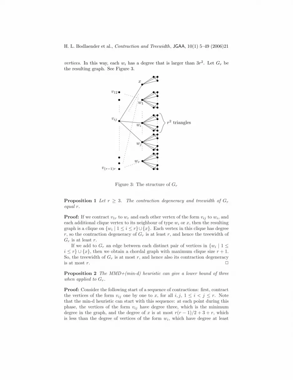
vertices. In this way, each wi has a degree that is larger than 3r2. Let Gr bethe resulting graph. See Figure 3.
vijwi
wj
x
v12
v(r−1)r
w1
wr
r2 triangles
Figure 3: The structure of Gr
Proposition 1 Let r ≥ 3. The contraction degeneracy and treewidth of Grequal r.
Proof: If we contract v1r to wr and each other vertex of the form vij to wi, andeach additional clique vertex to its neighbour of type wi or x, then the resultinggraph is a clique on wi | 1 ≤ i ≤ r∪x. Each vertex in this clique has degreer, so the contraction degeneracy of Gr is at least r, and hence the treewidth ofGr is at least r.
If we add to Gr an edge between each distinct pair of vertices in wi | 1 ≤i ≤ r ∪ x, then we obtain a chordal graph with maximum clique size r + 1.So, the treewidth of Gr is at most r, and hence also its contraction degeneracyis at most r. 2
Proposition 2 The MMD+(min-d) heuristic can give a lower bound of threewhen applied to Gr.
Proof: Consider the following start of a sequence of contractions: first, contractthe vertices of the form vij one by one to x, for all i, j, 1 ≤ i < j ≤ r. Notethat the min-d heuristic can start with this sequence: at each point during thisphase, the vertices of the form vij have degree three, which is the minimumdegree in the graph, and the degree of x is at most r(r − 1)/2 + 3 + r, whichis less than the degree of vertices of the form wi, which have degree at least
H. L. Bodlaender et al., Contraction and Treewidth, JGAA, 10(1) 5–49 (2006)22
3r2. So, during this first part of the running of the algorithm, the bound forthe contraction degeneracy is not larger than three.
After all vertices vij have been contracted to x, the graph has the followingform: x is adjacent to all wi; there are no edges between vertices wi, wi′ , i 6= i′;and then there are a number of four-cliques that have one vertex in commonwith the rest of the graph. This is a chordal graph with maximum clique sizefour. So, this graph has treewidth three, and hence contraction degeneracy atmost three. Hence, the min-d heuristic cannot give a bound larger than threein the remainder of the run of the algorithm. Thus, the maximum bound itobtains can be three. 2
Corollary 3 The MMD+(min-d) heuristic can give a solution that is a factorof Ω(
√n) away from optimal.
We can use cliques with four instead of three additional clique vertices. Inthat case, it holds that every possible run of the MMD+(min-d) heuristic givesa lower bound of four on the graph.
5.1.4 A bad example for the MMD+(least-c) heuristic
The example for the MMD+(least-c) heuristic is a modification of the one forthe min-d heuristic.
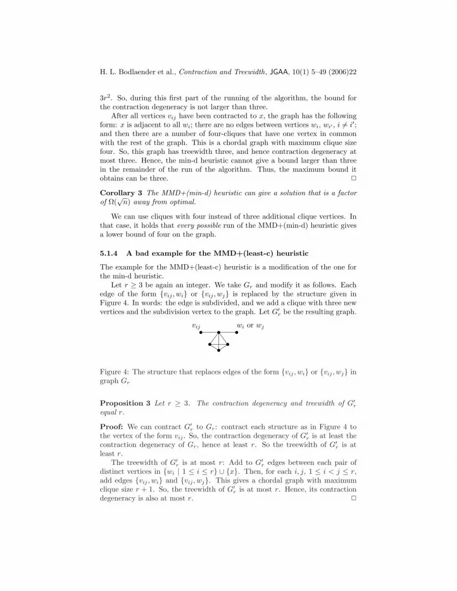
Let r ≥ 3 be again an integer. We take Gr and modify it as follows. Eachedge of the form vij , wi or vij , wj is replaced by the structure given inFigure 4. In words: the edge is subdivided, and we add a clique with three newvertices and the subdivision vertex to the graph. Let G′
r be the resulting graph.
vij wi or wj
Figure 4: The structure that replaces edges of the form vij , wi or vij , wj ingraph Gr
Proposition 3 Let r ≥ 3. The contraction degeneracy and treewidth of G′r
equal r.
Proof: We can contract G′r to Gr: contract each structure as in Figure 4 to
the vertex of the form vij . So, the contraction degeneracy of G′r is at least the
contraction degeneracy of Gr, hence at least r. So the treewidth of G′r is at
least r.The treewidth of G′
r is at most r: Add to G′r edges between each pair of
distinct vertices in wi | 1 ≤ i ≤ r ∪ x. Then, for each i, j, 1 ≤ i < j ≤ r,add edges vij , wi and vij , wj. This gives a chordal graph with maximumclique size r + 1. So, the treewidth of G′
r is at most r. Hence, its contractiondegeneracy is also at most r. 2

H. L. Bodlaender et al., Contraction and Treewidth, JGAA, 10(1) 5–49 (2006)23
Proposition 4 The MMD+(least-c) heuristic can give a bound of three whenapplied to G′
r.
Proof: Like for the min-d heuristic, the algorithm can start with contractingeach vertex of the form vij to x. During this phase, vertices vij have the mini-mum degree in the graph, namely three, and have no common neighbours withx. So, during this phase, the lower bound is set to three.
After all vertices of the form vij are contracted to x, the graph G′′ hastreewidth three. This can be seen as follows. The treewidth of a graph is themaximum treewidth of its biconnected components. The biconnected compo-nents of G′′ are either cliques with four vertices, single edges, or consist of x,a vertex wi, and a number of paths of length two between x and wi (for somei, 1 ≤ i ≤ r). In the first case, the treewidth of the component is three; in thelast case, the component has treewidth three. So, after the contractions of thevij-vertices to x, the bound of three cannot be increased. 2
Corollary 4 The MMD+(least-c) heuristic can give a solution that is a factorof Ω(
√n) away from optimal.
It is possible to modify the construction such that any run of theMMD+(least-c) heuristic gives a result far from optimal. Instead of cliqueswith three new vertices and one ‘old’ vertex, we use cliques with five new ver-tices and one old vertex. The structure of Figure 4 is replaced by the structureof Figure 5. In this way, we obtain a graph that has contraction degeneracy r,but for which any run of the MMD+(least-c) heuristic gives a lower bound thatis at most five.
vij wi or wj
Figure 5: An alternative structure that replaces edges of the form vij , wi orvij , wj in graph Gr
5.2 Heuristics for MCSLB With Contractions
Based on the result by Lucena [27] that the visited degree of an MCS orderingof G is a lower bound for the treewidth, we will look at heuristics based uponmaximum cardinality search and contraction.
For comparison, we have the MCSLB heuristic. This heuristic computes |V |MCS orderings ψ – one for each vertex as start vertex. It returns the maximumover these orderings of MCSLBψ, cf. [7].
The MCSLB+ heuristic starts by using MCSLB to find a start vertex wwith largest MCSLBψ. Then, we iteratively select a vertex and a neighbour tocontract, compute an MCS ordering, and repeat until the graph has no edges.

H. L. Bodlaender et al., Contraction and Treewidth, JGAA, 10(1) 5–49 (2006)24
To reduce the CPU time consumption, an MCS is carried out only with startvertex w (or vertices resulting from contractions that involve w) instead ofwith all possible start vertices. Three strategies for selecting a vertex v to becontracted are examined:
• min-deg selects a vertex of minimum degree.
• last-mcs selects the last vertex in the just computed MCS ordering.
• max-mcs selects a vertex with maximum visited degree in the just com-puted MCS ordering.
Once a vertex v is selected, we select a neighbour u of v using the two strate-gies min-d and least-c that are already explained for MMD+. We thus havesix versions of the MCSLB+ heuristic. These are experimentally evaluated inSection 6. We did not evaluate the MCSLB+(max-d) heuristic, because of thenegative experimental results for the MMD+(max-d) strategy.
5.3 Contraction and the LBN and LBP Heuristics
For each treewidth lower bound algorithm Y, we have two lower bound heuristicsLBN(Y) and LBP(Y), based on the technique by Clautiaux et al. [12], seeSection 2. So, we can have, e.g. the LBN(MMD+) algorithm.
A different method to combine the LBN or LBP methods with contractionis to alternate improvement steps with contractions. We describe the LBN+(Y)algorithm for some treewidth lower bound heuristic Y below. If we instead ofmaking a neighbours improved graph, take a paths improved graph, we obtainthe LBP+(Y) algorithm; the latter one is slower but often gives better bounds.
Algorithm LBN+(Y)1 Initialise L to some lower bound on the treewidth of G, e.g. L = 0.2 H := G.3 repeat4 H = the (L+ 1)-neighbours improved graph of H.5 b :=Y(H)6 if b > L7 then L := L+ 18 goto step 29 else select a vertex v of minimum degree in H.10 select neighbour u of v according to the least-c strategy.11 contract the edge u, v in H.12 endif13 until H is empty14 output L.
In the description above, we used the least-c strategy, as this one performedbest for the other heuristics; of course, variants with other contraction strategiescan also be considered.
H. L. Bodlaender et al., Contraction and Treewidth, JGAA, 10(1) 5–49 (2006)25
Proposition 5 If algorithm Y is an algorithm that outputs a lower bound onthe treewidth of its input graph, then LBN+(Y) and LBP+(Y) output lowerbounds on the treewidth of its input graph.
Proof: Let G be the input graph of algorithm LBN+(Y) or LBP+(Y). Aninvariant of the algorithm is that the treewidth of G is at least L. A secondinvariant of the algorithm is that when the treewidth of G equals L, then thetreewidth of H is at most L. Clearly, these invariants hold initially. Lemmas 1and 2 show that the second invariant holds also after making an improved graphin step 4. The fact that contraction cannot increase treewidth shows that thesecond invariant holds after a contraction in step 11. Similar as in [12], whenY outputs a value larger than L on H, then the treewidth of H and hence thetreewidth of G (by the second invariant) is larger than L, so increasing L byone in step 7 maintains the first invariant. 2
In our experiments, we started the algorithm by setting the lower bound Lto the value computed by the MMD+ heuristic.
5.3.1 Faster Implementation of LBP+
A straightforward implementation of an LBP+(Y) heuristic can be very slow.However, we can observe that some steps are not necessary. Contracting an edgecan increase the number of vertex disjoint paths between two vertices, but notfor all pairs. Lemma 5 tells us that contracting an edge x, y cannot increasethe number of vertex disjoint paths between u and v, if x, y ∩ u, v = ∅.
Lemma 5 Let be given vertices u and v and edge e = x, y in G = (V,E).Furthermore, let N be the maximum number of vertex disjoint paths between uand v in G, and let N ′ be the maximum number of vertex disjoint paths betweenu and v in G/x, y. Then we have:
x, y ∩ u, v = ∅ =⇒ N ′ ≤ N
Proof: Let ae be the new vertex created by contracting edge e. We consider aset P ′ of vertex disjoint paths p1, ..., pN ′ between u and v in G/e. Since thesepaths are vertex disjoint and x, y ∩ u, v = ∅, there can be at most one pathp′ in P ′ going through the new vertex ae, i.e. ae is contained in at most onepath p′ of P ′.
One easily sees that there is a path p in G between u and v that uses allvertices of p′ except ae and x and/or y. Therefore, we have a set P of N ′ vertexdisjoint paths between u and v in G. Hence, N ′ ≤ N . 2
In other words, the number of vertex disjoint paths between u and v can beincreased by an edge contraction, only if an edge incident to u or v is contracted.A consequence of this is that after contracting edge e which results in a newvertex ae, we only have to look for the number of vertex disjoint paths of pairsof vertices that contain ae. This results in a drastic speed up compared tothe case when checking all pairs of vertices for L + 1 vertex disjoint paths, as

H. L. Bodlaender et al., Contraction and Treewidth, JGAA, 10(1) 5–49 (2006)26
we check O(n) pairs instead of Θ(n2) pairs. However, once we have found animprovement edge in the graph, we then must check all other pairs, as possibly,after an improvement edge is added, pairs of vertices that do not contain ae canhave L+ 1 vertex disjoint paths.
5.3.2 LBN+(MD) versus LBN+(MMD)
We now compare the LBN+(MD) heuristic with the LBN+(MMD) heuristic,and similarly, the LBP+(MD) heuristic with the LBP+(MMD) heuristic. Weshow that these output the same lower bound result. I.e. in the LBN+(MD)heuristic, we just use the minimum degree of a vertex in H as lower bound,while in the LBN+(MMD) heuristic, we compute the degeneracy.
The intuitive idea is that LBN+(MD) and LBN+(MMD) compute the sameresult because, due to the additional contraction step, the subgraphs consideredby the MMD lower bound, will also be considered in the algorithm LBN+(MD);similarly for the version with paths improvement. Below, we show that thisintuition is correct. However, before that, we give one lemma.
Lemma 6 (See [36].) Let be given a graph G = (V,E), vertex v ∈ V and edgee ∈ E. Furthermore, let ae be the resulting new vertex after contracting edge e.If v 6∈ e, then dG/e(v) ≥ dG(v) − 1. If v ∈ e, then dG/e(ae) ≥ dG(v) − 1.
Lemma 7 Let G = (V,E) be a graph. Let the result of running theLBN+(MD), LBN+(MMD), LBP+(MD) and LBP+(MMD) algorithms on Gbe respectively αn, βn, αp and βp. Then αn = βn and αp = βp.
Proof: The proof is the same for the versions with neighbours and paths im-provement. Thus, in the proof below, we write LBX+(MD) and LBX+(MMD),where the X can stand for N or P, and we drop the subscripts n and p from αand β.
First note that when the LBX+(MD) and LBX+(MMD) enter the loop atstep three with the same value of L, then they will work with the same graphH. Thus, we have that α ≤ β: when LBX+(MD) increases L by one, we havethat L is smaller than the minimum degree of H, hence also smaller than thedegeneracy of H, and hence the LBX+(MMD) algorithm will also increase Lby one at the corresponding point during the execution of the algorithms. Toshow equality, we assume the following, and we will derive a contradiction:
α < β (1)
Consider the moments step 2 is done by algorithm LBX+(MMD) and byalgorithm LBX+(MD) when L = α. As LBX+(MD) outputs α, this is thelast time step 2 is done by the LBX+(MD) algorithm, while the LBX+(MMD)algorithm will increase L further (as α < β), and hence will execute later the‘goto step 2’ command at least once.
Let H∗ be the the graph H at the moment the LBX+(MMD) algorithm isat step 7 and 8 when the algorithm increases L from α to α + 1. This graph

H. L. Bodlaender et al., Contraction and Treewidth, JGAA, 10(1) 5–49 (2006)27
H∗ is formed from G by a sequence of contractions and (α + 1)-neighbours or(α+1)-paths improvement steps. As the test in step 6 was true, the degeneracyof H∗ is at least α+ 1.
The LBX+(MD) algorithm has started a run of the main iteration withL = α. As the algorithm outputs α, this is its last iteration. During thisiteration, it does the same improvement steps as the LBX+(MMD) algorithm,and hence, at some point, creates the graph H∗. However, it cannot executesteps 7 and 8 now, so the test in step 6 was false for the LBX+(MD) algorithms.Thus, we have:
δ(H∗) ≤ α < δD(H∗)
Write d = δD(H∗). Therefore, there exists an induced subgraph H ′ ⊂ H∗ with
δ(H∗) < δ(H ′) = d
Note that all vertices in V (H ′) have degree at least d := δD(H∗) in H∗. Wenow consider the execution of LBX+(MD), starting when H is the graph H∗,up to just before the point that the first vertex from H ′ is selected as minimumdegree vertex v in step 9. During this part of the execution, we have that H ′ isa subgraph of the graph H used by the algorithm: improvement steps only addedges, and no edges between vertices in H ′ are contracted.
Now, consider the first vertex v∗ from H ′ that is selected as minimum degreevertex v in step 9 by LBX+(MD). As H ′ is a subgraph of the graph H, we havethat the degree of v∗ at the moment it is selected is at least its degree in H ′,which is at least d. But, as v∗ is the minimum degree of a vertex in H, allvertices in H have at this point degree at least d. This gives a contradiction:consider the test at step 6 just before v∗ was selected: the minimum degree ofH is at least d, which is larger than the current value of L, i.e. α. So, this testis true, and the algorithm will increase L, contradiction.
So, we can conclude that the assumption α < β is false, hence α = β. 2
Whether in practice LBX+(MD) would be more time-efficient thanLBX+(MMD) is unclear from the above. The lower bound MMD is more timeconsuming than MD, but can result in a b > L earlier during the contractionprocess, by this avoiding a number of graph improvement steps. By Lemma 7,the number of graph improvement steps in the last iteration will be equal, slow-ing down the algorithm on this point.
Similarly LBX+(MMD+) can be more time-efficient than LBX+(MD):MMD+ is more time consuming but can reduce the number of improvementsteps. Moreover, LBX+(MMD+) can return a better bound than LBX+(MD),although this rarely happens. Experimental results with LBX+(MD),LBX+(MMD), and LBX+(MMD+) have shown that the computation timesof LBX+(MD) are significantly smaller than those for LBX+(MMD) which ontheir turn are significantly smaller than those for LBX+(MMD+).

H. L. Bodlaender et al., Contraction and Treewidth, JGAA, 10(1) 5–49 (2006)28
6 Experimental Results
In this section, we report on the results of computational experiments we havecarried out. We tested our algorithms on a number of graphs. The first setof instances are probabilistic networks from existing decision support systemsfrom fields like medicine and agriculture. Central to the use of these networks isto solve the probabilistic inference problem. One of the most used methods forprobabilistic inference is the following: one constructs the so-called moralisedgraph from the probabilistic network. After this (simple) step, one builds atree decomposition of the moralised graph, and then uses this tree decomposi-tion to solve the probabilistic inference problem. The time for the last step isexponential in the width of the tree decomposition, but linear in the numberof nodes. Thus, computing the treewidth of these moralised graphs is of greatpractical use. The second set of instances are from frequency assignment prob-lems from the EUCLID CALMA project. In [21, 23], tree decompositions wereused to solve the frequency assignment problem on many of the networks fromthis collection of instances. In addition, we use versions of the network, ob-tained by preprocessing [9]. The preprocessing algorithm changed the instancesto equivalent instances of smaller size. We have also used these sets of instancesin earlier experiments. A third set of instances are taken from the work ofCook and Seymour [14]. Here, they present a heuristic for the travelling sales-man problem where they use branch decompositions (a notion strongly relatedto tree decompositions) of graphs formed by merging a number of TSP-tours.Finally, we computed the lower bounds for many of the DIMACS colouring in-stances [16]. Among all these, we excluded those networks for which the MMDheuristic already gives the exact treewidth. Some of the graphs can be obtainedfrom [35]. All algorithms have been written in C++, and the computationshave been carried out on a Linux operated PC with a 3.0 GHz Intel Pentium 4processor. The CPU time is measured in seconds.
Tables 2, 3 and 4 give the results for some selected instances, whose behav-iour is typical for the entire set of instances. In the appendix, we give longertables for the entire collection of graphs we tested our algorithms on. In Ta-ble 2, we included the best known upper bound (UB) for comparison [22, 13].For the six variants of the MCSLB+ algorithm we give for space reasons onlythe average time. There were no large differences in the running times betweenthe different MCSLB+ heuristics. Lucena [26] also has made an experimentalevaluation of the MCSLB+ algorithm.
We can see from these results that contraction is a very useful method forobtaining lower bounds for treewidth. The improvements obtained by usingMMD+ instead of MMD, or MCSLB+ instead of MCSLB are in many casesquite significant.
Concerning the different strategies for MMD+, we can observe that the least-c strategy is best. In many cases, it performs much better than the other twostrategies, and in all our experiments, there is only one case where its bound isone smaller than that obtained with the min-d strategy. The max-d strategyappears to do badly, giving in general much smaller lower bounds than the other

H. L. Bodlaender et al., Contraction and Treewidth, JGAA, 10(1) 5–49 (2006)29
two. Thus, we did not use this strategy for the other heuristics.For the MCSLB+, again the least-c strategy seems to be better than the min-
d strategy. We observe that min-deg and last-mcs for selecting the contractionvertex, combined with least-c outperform the other strategies. The differencesbetween MMD+(least-c) and MCSLB+(least-c) are usually small, but in a fewcases, the MCSLB+(least-c) gives a significant larger bound. The time of theseheuristic is often much larger than that of the MMD+ heuristics.
In Table 4 a number of LBN and LBP strategies are compared. Here,MMD+(least-c) and MCSLB+(min-deg,least-c) are used as subroutines. ForLBX(MMD) and LBX(MCSLB), the LBP variants provide significantly betterbounds than the LBN variants. Time consumption however is also significantlyhigher. For LBX(MMD+) and LBX(MCSLB+), there is only marginal differ-ences between LBN and LBP. Moreover, LBN(MMD+) and LBN(MCSLB+)are typically as good as or even better than LBP(MMD) and LBP(MCSLB),whereas there computation times are lower. Although, MCSLB and MCSLB+provide slightly better bounds than MMD and MMD+ respectively, the resultsshow that it is not worth to include them in LBX strategies instead of MMDand MMD+: the additional computational effort is huge in comparison to thegain in the lower bound.
For the instances from probabilistic networks and frequency assignment, theLBN+(MD) and LBP+(MD) algorithm give often rather significant increases tothe lower bounds, but often at the cost of more time use. The situation for theTSP-instances is interesting. The LBN(MMD+) and LBP+(MD) algorithmsseem to give the best tradeoff between lower bound and running time. TheLBP+(MD) algorithm appears to use very much time on these instances. A fewcases could not be run to completion due to the large time used; others give aresult only after several hours of computation time.
We can also observe that in a several cases (e.g. link, munin3) theLBP+(MD) algorithm performs faster than the LBP(MMD). This can be ex-plained by the fact that the LBP+(MD) algorithm starts with the lower boundvalue given by the MMD+ algorithm, while the LBP(MMD) algorithm startswith the value provided by the MMD algorithm. Thus, these latter algorithmshave more rounds, and as often many improvements are possible for small valuesof k, the earlier rounds are often more time consuming. Hence, for speeding upLBN, LBP, LBN+ or LBP+ based heuristics, one should start with a good startvalue of the lower bound. For instance, one might want to start an LBP+(MD)heuristic with a lower bound obtained by an LBN+(MD) heuristic.
For the class of instances derived from the work of Cook and Seymour [14],our heuristics seem not well suited. This can be explained as follows. For planargraphs, the contraction degeneracy is at most five (as planar graphs and henceminors of planar graphs have always a vertex of degree at most five). The TSP-instances can be expected to be close to planar; thus one can expect the MMD+based heuristics not to do well on such instances in general.
Overall, for 45 out of 151 graphs, the best lower bound computed equals thebest known upper bound, for many other instances the remaining gap is verysmall. From these results, we can conclude that combining existing methods

H. L. Bodlaender et al., Contraction and Treewidth, JGAA, 10(1) 5–49 (2006)30
with contraction can give considerable improvements of treewidth lower bounds.As illustrated by Figure 6, the MMD+(least-c) appears to be a good algorithmwith often (almost) negligible running times and good bounds; better boundscan be obtained by slower algorithms, like LBN+(MD) or LBP+(MD).
instance size UB MMD MMD+min-d max-d least-c
|V | |E| LB CPU LB CPU LB CPU LB CPU
link 724 1738 13 4 0.00 8 0.02 5 0.01 11 0.03munin1 189 366 11 4 0.00 8 0.01 5 0.00 10 0.00munin3 1044 1745 7 3 0.01 7 0.01 4 0.02 7 0.02pignet2 3032 7264 135 4 0.01 29 0.11 10 0.07 38 0.20celar06 100 350 11 10 0.00 11 0.00 10 0.00 11 0.01celar07pp 162 764 16 11 0.00 13 0.00 12 0.00 15 0.01graph04 200 734 55 6 0.00 12 0.01 7 0.00 19 0.02rl5934-pp 904 1800 21 3 0.01 5 0.02 4 0.02 5 0.03queen15-15 225 5180 171 42 0.00 52 0.07 42 0.02 58 0.19
Table 2: Upper bounds and results of MMD and MMD+ for selected instances
instance MCSLB MCSLB+ LBsmin-deg last-mcs max-mcs average
LB CPU min-d least-c min-d least-c min-d least-c CPU
link 5 3.09 8 10 8 11 8 6 43.08munin1 4 0.17 8 10 9 10 9 7 0.95munin3 4 5.87 6 7 7 7 6 7 33.80pignet2 5 59.60 28 39 30 39 16 18 509.60celar06 11 0.06 11 11 11 11 11 11 0.33celar07pp 12 0.16 14 15 13 15 13 15 1.22graph04 8 0.25 12 20 13 20 14 16 1.95rl5934-pp 4 8.27 5 6 5 6 5 6 35.98queen15-15 42 1.80 52 59 52 62 52 58 27.79
Table 3: Results of MCSLB+ for selected instances
7 Discussion and Concluding Remarks
In this article, we examined the notion of contraction degeneracy, and severalheuristics for treewidth lower bounds which are based on the combination ofcontraction with existing treewidth lower bound methods. We showed somecorresponding decision problems to be NP-complete, but also introduced severalheuristics.
The practical experiments show that contracting edges is a very good ap-proach for obtaining lower bounds for treewidth as it considerably improves

H.L.B
odlaen
der
etal.,
Contra
ction
and
Treew
idth
,JG
AA
,10(1)
5–49(2006)31
instance LBN LBN LBN LBN LBN+ LBP LBP LBP LBP LBP+(MMD) (MCSLB) (MMD+) (MCSLB+) (MD) (MMD) (MCSLB) (MMD+) (MCSLB+) (MD)LB CPU LB CPU LB CPU LB CPU LB CPU LB CPU LB CPU LB CPU LB CPU LB CPU
link 4 0.04 5 8.03 11 0.05 10 127.37 11 0.40 10 2525.67 10 623.78 11 10.93 11 223.65 12 40.70munin1 4 0.00 4 0.45 10 0.01 10 2.00 10 0.03 7 3.70 7 4.88 10 0.10 10 2.12 10 0.16munin3 3 0.09 4 15.11 7 0.04 7 69.88 7 0.53 6 3747.90 6 265.25 7 15.88 7 88.35 7 31.31pignet2 6 2.86 6 240.24 38 0.28 39 1051.52 41 21.58 - - - - 40 144.83 39 1091.67 48 1280.96celar06 10 0.00 11 0.15 11 0.01 11 0.81 11 0.02 11 0.29 11 0.23 11 0.09 11 0.89 11 0.12celar07pp 13 0.02 13 0.68 15 0.01 15 3.16 15 0.06 15 7.64 15 6.48 15 0.80 15 3.96 16 2.11graph04 6 0.01 8 0.68 20 0.03 20 4.30 21 0.34 10 194.32 10 10.81 20 0.03 20 4.27 24 4.34rl5934-pp 3 0.14 4 11.93 5 0.05 6 61.69 3 0.55 - - - - 6 5.86 6 56.51 9 38137.20queen15-15 42 0.08 42 2.37 58 0.24 59 32.85 60 7.36 48 1045.63 50 1221.13 58 0.24 59 32.01 73 7579.01
Table 4: Results of LBN+/LBP+ for selected instances

H. L. Bodlaender et al., Contraction and Treewidth, JGAA, 10(1) 5–49 (2006)32
Figure 6: CPU time (logarithmic scale) vs. lower bounds for instance queen15-15 (for MMD+ and MCSLB+ only MMD+(least-c) and MCSLB+(min-deg,least-c) are shown)
known lower bounds. The MMD+ heuristics appear to be attractive, due tothe fact that the running time of these heuristics is almost always negligible,and the bound is reasonably good. The MCSLB+ heuristics have much largerrunning time, and often give only a small improvement on the MMD+ basedlower bound. Several LBN, LBP, and LBN+ heuristics often use more time thanthe MMD+, but less than the MCSLB+, and can give further lower bound im-provements, cf. Figure 6. The LBP+(MD) heuristic usually is slowest but givesoften the best results. Furthermore, we see that the strategy for selecting aneighbour u of v with the least number of common neighbours of u and v oftenperforms best and appears to be the clear choice for such a strategy.
Notice that although the gap between lower and upper bound could be sig-nificantly closed by contracting edges within the algorithms, the absolute gapis still large for many graphs (pignet2, graph*). While it is known that thetreewidth has polynomial time approximation algorithm with logarithmic per-formance ratios, the existence of polynomial time approximation algorithms fortreewidth with constant bounded ratios remains a long standing open problem.Thus, obtaining good lower bounds for treewidth is both from a theoretical asfrom a practical viewpoint a highly interesting topic for further research.
A different lower bound for treewidth was provided by Ramachandramurthi[28, 29]. While this lower bound appears to generally give small lower boundvalues, it can also be combined with contraction, see [24] for a recently publishedstudy. Moreover, in [6], a new lower bound heuristic has been recently developedfor (close-to) planar graphs, where contraction-based lower bounds seems to beless lucrative.
Apart from its function as a treewidth lower bound, the contraction degen-eracy appears to be an attractive and elementary graph measure, worth further

H. L. Bodlaender et al., Contraction and Treewidth, JGAA, 10(1) 5–49 (2006)33
study. For instance, interesting topics are its computational complexity on spe-cial graph classes or the complexity of approximation algorithms with a guar-anteed performance ratio. We recently found a polynomial time algorithm forcographs [10], and we observed that the problem is easy for chordal graphs [36],but many other cases remain open.
Acknowledgements
We would like to thank Dieter Kratsch for useful discussions and also the anony-mous referees of this article.

H. L. Bodlaender et al., Contraction and Treewidth, JGAA, 10(1) 5–49 (2006)34
References
[1] S. Arnborg, D. G. Corneil, and A. Proskurowski. Complexity of findingembeddings in a k-tree. SIAM J. Algebraic Discrete Methods, 8:277–284,1987.
[2] S. Arnborg and A. Proskurowski. Characterization and recognition of par-tial 3-trees. SIAM J. Algebraic Discrete Methods, 7:305–314, 1986.
[3] H. L. Bodlaender. A linear time algorithm for finding tree-decompositionsof small treewidth. SIAM J. Computing, 25:1305–1317, 1996.
[4] H. L. Bodlaender. A partial k-arboretum of graphs with bounded treewidth.Theoretical Computer Science, 209:1–45, 1998.
[5] H. L. Bodlaender. Necessary edges in k-chordalizations of graphs. Journalof Combinatorial Optimization, 7:283–290, 2003.
[6] H. L. Bodlaender, A. Grigoriev, and A. M. C. A. Koster. Treewidth lowerbounds with brambles. In G. S. Brodal and S. Leonardi, editors, Proceedings13th Annual European Symposium on Algorithms, ESA2005, pages 391–402. Springer Verlag, Lecture Notes in Computer Science, vol. 3669, 2005.
[7] H. L. Bodlaender and A. M. C. A. Koster. On the Maximum CardinalitySearch lower bound for treewidth. In J. Hromkovic, M. Nagl, and B. West-fechtel, editors, Proc. 30th International Workshop on Graph-TheoreticConcepts in Computer Science WG 2004, pages 81–92. Springer Verlag,Lecture Notes in Computer Science, vol. 3353, 2004.
[8] H. L. Bodlaender and A. M. C. A. Koster. Safe separators for treewidth.In Proceedings 6th Workshop on Algorithm Engineering and ExperimentsALENEX04, pages 70–78, 2004.
[9] H. L. Bodlaender, A. M. C. A. Koster, and F. v. d. Eijkhof. Pre-processingrules for triangulation of probabilistic networks. Computational Intelli-gence, 21(3):286–305, 2005.
[10] H. L. Bodlaender and T. Wolle. Contraction degeneracy on cographs. Tech-nical Report UU-CS-2004-031, Institute for Information and ComputingSciences, Utrecht University, Utrecht, The Netherlands, 2004.
[11] J. A. Bondy and U. S. R. Murty. Graph Theory with Applications. AmericanElsevier, MacMillan, New York, London, 1976.
[12] F. Clautiaux, J. Carlier, A. Moukrim, and S. Negre. New lower and up-per bounds for graph treewidth. In J. D. P. Rolim, editor, ProceedingsInternational Workshop on Experimental and Efficient Algorithms, WEA2003, pages 70–80. Springer Verlag, Lecture Notes in Computer Science,vol. 2647, 2003.

H. L. Bodlaender et al., Contraction and Treewidth, JGAA, 10(1) 5–49 (2006)35
[13] F. Clautiaux, A. Moukrim, S. Negre, and J. Carlier. Heuristic and meta-heuristic methods for computing graph treewidth. RAIRO Operations Re-search, 38:13–26, 2004.
[14] W. Cook and P. D. Seymour. Tour merging via branch-decomposition.Informs J. on Computing, 15(3):233–248, 2003.
[15] B. Courcelle. The monadic second-order logic of graphs I: Recognizablesets of finite graphs. Information and Computation, 85:12–75, 1990.
[16] The second DIMACS implementation challenge: NP-Hard Prob-lems: Maximum Clique, Graph Coloring, and Satisfiability. Seehttp://dimacs.rutgers.edu/Challenges/, 1992–1993.
[17] R. G. Downey and M. R. Fellows. Parameterized Complexity. Springer,1998.
[18] F. v. d. Eijkhof and H. L. Bodlaender. Safe reduction rules for weightedtreewidth. In L. Kucera, editor, Proceedings 28th Int. Workshop on GraphTheoretic Concepts in Computer Science, WG’02, pages 176–185. SpringerVerlag, Lecture Notes in Computer Science, vol. 2573, 2002.
[19] M. R. Garey and D. S. Johnson. Computers and Intractability, A Guide tothe Theory of NP-Completeness. W.H. Freeman and Company, New York,1979.
[20] V. Gogate and R. Dechter. A complete anytime algorithm for treewidth.In Proceedings of the 20th Annual Conference on Uncertainty in ArtificialIntelligence UAI-04, pages 201–208, Arlington, Virginia, USA, 2004. AUAIPress.
[21] A. M. C. A. Koster. Frequency Assignment - Models and Algorithms. PhDthesis, Univ. Maastricht, Maastricht, The Netherlands, 1999.
[22] A. M. C. A. Koster, H. L. Bodlaender, and S. P. M. van Hoesel. Treewidth:Computational experiments. In H. Broersma, U. Faigle, J. Hurink, andS. Pickl, editors, Electronic Notes in Discrete Mathematics, volume 8, pages54–57. Elsevier Science Publishers, 2001.
[23] A. M. C. A. Koster, S. P. M. van Hoesel, and A. W. J. Kolen. Solvingpartial constraint satisfaction problems with tree decomposition. Networks,40:170–180, 2002.
[24] A. M. C. A. Koster, T. Wolle, and H. L. Bodlaender. Degree-basedtreewidth lower bounds. In S. E. Nikoletseas, editor, Proceedings of the 4thInternational Workshop on Experimental and Efficient Algorithms WEA2005, pages 101–112. Springer Verlag, Lecture Notes in Computer Science,vol. 3503, 2005.

H. L. Bodlaender et al., Contraction and Treewidth, JGAA, 10(1) 5–49 (2006)36
[25] S. J. Lauritzen and D. J. Spiegelhalter. Local computations with probabil-ities on graphical structures and their application to expert systems. TheJournal of the Royal Statistical Society. Series B (Methodological), 50:157–224, 1988.
[26] B. Lucena. Dynamic Programming, Tree-Width, and Computation onGraphical Models. PhD thesis, Brown University, Providence, RI, USA,2002.
[27] B. Lucena. A new lower bound for tree-width using maximum cardinalitysearch. SIAM J. Discrete Mathematics, 16:345–353, 2003.
[28] S. Ramachandramurthi. A lower bound for treewidth and its consequences.In E. W. Mayr, G. Schmidt, and G. Tinhofer, editors, Proceedings 20thInternational Workshop on Graph Theoretic Concepts in Computer ScienceWG’94, pages 14–25. Springer Verlag, Lecture Notes in Computer Science,vol. 903, 1995.
[29] S. Ramachandramurthi. The structure and number of obstructions totreewidth. SIAM J. Discrete Mathematics, 10:146–157, 1997.
[30] N. Robertson and P. D. Seymour. Graph minors. XIII. The disjoint pathsproblem. J. Combinatorial Theory Series B, 63:65–110, 1995.
[31] N. Robertson and P. D. Seymour. Graph minors. XX. Wagner’s conjecture.J. Combinatorial Theory Series B, 92:325–357, 2004.
[32] N. Robertson, P. D. Seymour, and R. Thomas. Quickly excluding a planargraph. J. Combinatorial Theory Series B, 62:323–348, 1994.
[33] K. Shoikhet and D. Geiger. A practical algorithm for finding optimal tri-angulations. In Proc. National Conference on Artificial Intelligence (AAAI’97), pages 185–190. Morgan Kaufmann, 1997.
[34] R. E. Tarjan and M. Yannakakis. Simple linear time algorithms to testchordiality of graphs, test acyclicity of graphs, and selectively reduce acyclichypergraphs. SIAM J. Computing, 13:566–579, 1984.
[35] Treewidthlib. http://www.cs.uu.nl/people/hansb/treewidthlib, 2004.
[36] T. Wolle and H. L. Bodlaender. A note on edge contraction. TechnicalReport UU-CS-2004-028, Institute of Information and Computing Sciences,Utrecht University, Utrecht, The Netherlands, 2004.

H. L. Bodlaender et al., Contraction and Treewidth, JGAA, 10(1) 5–49 (2006)37
A All Computational Results
Below, we present the results of our experiments. Earlier, we presented a numberof selected results. See Section 6 for details on the backgrounds of the graphsand the experimental setting.
instance size UB MMD MMD+min-d max-d least-c
|V | |E| LB CPU LB CPU LB CPU LB CPU
barley 48 126 7 5 0.00 6 0.00 5 0.00 6 0.00diabetes 413 819 4 3 0.00 4 0.01 4 0.00 4 0.00link 724 1738 13 4 0.00 8 0.02 5 0.01 11 0.03mildew 35 80 4 3 0.00 4 0.00 3 0.00 4 0.00munin1 189 366 11 4 0.00 8 0.01 5 0.00 10 0.00munin2 1003 1662 7 3 0.01 6 0.01 4 0.01 6 0.02munin3 1044 1745 7 3 0.01 7 0.01 4 0.02 7 0.02munin4 1041 1843 8 4 0.01 7 0.01 5 0.01 7 0.02oesoca+ 67 208 11 9 0.00 9 0.00 9 0.00 9 0.00oow-trad 33 72 6 3 0.00 4 0.00 4 0.00 5 0.00oow-bas 27 54 4 3 0.00 4 0.00 3 0.00 4 0.00oow-solo 40 87 6 3 0.00 4 0.00 4 0.00 5 0.00pathfinder 109 211 6 5 0.00 6 0.00 5 0.00 6 0.01pignet2 3032 7264 135 4 0.01 29 0.11 10 0.07 38 0.20pigs 441 806 10 3 0.00 6 0.01 4 0.00 7 0.01ship-ship 50 114 8 4 0.00 6 0.00 4 0.00 6 0.00water 32 123 9 6 0.00 7 0.00 7 0.00 8 0.00wilson 21 27 3 2 0.00 3 0.00 3 0.00 3 0.00
barley-pp 26 78 7 5 0.00 6 0.00 5 0.00 6 0.00link-pp 308 1158 13 6 0.00 8 0.01 6 0.00 11 0.02munin1-pp 66 188 11 4 0.00 8 0.00 5 0.00 10 0.01munin2-pp 167 455 7 4 0.00 6 0.01 5 0.00 6 0.01munin3-pp 96 313 7 4 0.00 7 0.00 5 0.00 7 0.01munin4-pp 217 646 8 5 0.00 7 0.00 5 0.01 8 0.01munin-kgo-pp 16 41 5 4 0.00 4 0.00 5 0.00 4 0.00oesoca+-pp 14 75 11 9 0.00 10 0.00 9 0.00 9 0.00oow-trad-pp 23 54 6 4 0.00 5 0.00 4 0.00 5 0.00oow-solo-pp 27 63 6 4 0.00 5 0.00 4 0.00 5 0.00pathfinder-pp 12 43 6 5 0.00 6 0.00 5 0.00 6 0.00pignet2-pp 1024 3774 132 5 0.01 29 0.09 10 0.03 38 0.13pigs-pp 48 137 10 4 0.00 7 0.00 4 0.00 7 0.00ship-ship-pp 30 77 8 4 0.00 6 0.00 4 0.00 6 0.00water-pp 22 96 9 6 0.00 8 0.00 7 0.00 8 0.00
Table 5: Upper bounds and results of MMD and MMD+ for (preprocessedversions of) probabilistic networks

H. L. Bodlaender et al., Contraction and Treewidth, JGAA, 10(1) 5–49 (2006)38
instance size UB MMD MMD+min-d max-d least-c
|V | |E| LB CPU LB CPU LB CPU LB CPU
celar01 458 1449 15 8 0.00 12 0.01 9 0.00 14 0.02celar02 100 311 10 9 0.00 9 0.00 9 0.00 10 0.00celar03 200 721 15 8 0.00 11 0.00 9 0.00 13 0.01celar04 340 1009 16 9 0.00 12 0.01 9 0.00 13 0.01celar05 200 681 15 9 0.01 11 0.00 9 0.00 13 0.01celar06 100 350 11 10 0.00 11 0.00 10 0.00 11 0.01celar06pp 82 327 11 10 0.00 11 0.00 10 0.00 11 0.01celar07 200 817 16 11 0.00 13 0.00 12 0.01 15 0.00celar07pp 162 764 16 11 0.00 13 0.00 12 0.00 15 0.01celar08 458 1655 16 11 0.00 13 0.01 12 0.01 15 0.01celar08pp 365 1539 16 11 0.00 13 0.00 12 0.01 15 0.01celar09 340 1130 16 11 0.01 13 0.01 12 0.00 15 0.01celar10 340 1130 16 11 0.00 13 0.01 12 0.01 15 0.01celar11 340 975 15 8 0.00 11 0.00 9 0.00 13 0.01graph01 100 358 24 8 0.00 9 0.01 9 0.00 14 0.00graph02 200 709 50 6 0.00 11 0.00 7 0.01 20 0.02graph03 100 340 22 5 0.00 8 0.00 6 0.01 14 0.00graph04 200 734 55 6 0.00 12 0.01 7 0.00 19 0.02graph05 100 416 25 8 0.00 9 0.00 9 0.00 15 0.00graph06 200 843 53 8 0.00 12 0.01 9 0.00 21 0.02graph06pp 119 348 17 5 0.00 7 0.00 6 0.00 11 0.01graph07 200 843 53 8 0.00 12 0.01 9 0.00 21 0.02graph08 340 1234 91 7 0.00 16 0.02 8 0.01 26 0.04graph09 458 1667 116 8 0.01 17 0.03 9 0.01 29 0.06graph10 340 1275 93 6 0.00 15 0.01 7 0.01 27 0.04graph11 340 1425 98 7 0.00 17 0.01 8 0.01 27 0.05graph11pp 340 1424 98 7 0.00 16 0.02 8 0.01 28 0.05graph12 340 1256 90 5 0.00 16 0.01 6 0.01 25 0.04graph13 458 1877 126 6 0.00 18 0.02 7 0.01 31 0.07graph13pp 456 1874 130 6 0.01 18 0.03 7 0.01 31 0.07graph14 458 1398 121 4 0.00 20 0.02 8 0.02 27 0.05
Table 6: Upper bounds and results of MMD and MMD+ for frequency assign-ment instances

H. L. Bodlaender et al., Contraction and Treewidth, JGAA, 10(1) 5–49 (2006)39
instance size UB MMD MMD+min-d max-d least-c
|V | |E| LB CPU LB CPU LB CPU LB CPU
celar01-pp 157 804 15 8 0.00 12 0.00 9 0.00 14 0.01celar02-pp 19 115 10 9 0.00 9 0.00 9 0.00 10 0.00celar03-pp 81 413 15 9 0.00 11 0.01 10 0.00 13 0.00celar04-pp 114 524 16 9 0.00 12 0.00 10 0.00 13 0.01celar05-pp 80 426 15 9 0.00 12 0.00 9 0.01 13 0.00celar07-pp 92 521 16 11 0.00 13 0.01 11 0.00 15 0.00celar08-pp 189 1016 16 11 0.00 13 0.01 12 0.00 15 0.01celar09-pp 133 646 16 11 0.00 13 0.00 11 0.00 15 0.01celar10-pp 133 646 16 11 0.01 13 0.01 11 0.00 15 0.01celar11-pp 96 470 15 9 0.00 11 0.00 9 0.01 13 0.00graph01-pp 89 332 24 8 0.00 10 0.00 9 0.01 15 0.00graph02-pp 179 659 48 6 0.00 12 0.01 7 0.01 20 0.01graph03-pp 79 293 22 6 0.00 8 0.00 6 0.01 13 0.00graph04-pp 179 678 53 6 0.01 12 0.00 7 0.01 19 0.01graph05-pp 91 394 25 8 0.00 9 0.01 9 0.00 15 0.01graph06-pp 180 790 52 8 0.00 13 0.01 9 0.00 21 0.02graph07-pp 180 790 52 8 0.00 13 0.01 9 0.00 21 0.02graph08-pp 314 1173 90 7 0.01 16 0.02 8 0.01 26 0.04graph09-pp 405 1525 116 8 0.00 18 0.04 9 0.02 29 0.08graph10-pp 328 1253 97 6 0.00 16 0.03 7 0.01 26 0.05graph11-pp 307 1338 93 7 0.00 16 0.02 8 0.01 28 0.04graph12-pp 312 1177 87 6 0.00 16 0.02 7 0.01 25 0.03graph13-pp 420 1772 129 6 0.01 19 0.03 7 0.01 31 0.07graph14-pp 395 1325 127 5 0.00 20 0.02 8 0.02 27 0.04
Table 7: Upper bounds and results of MMD and MMD+ for preprocessed ver-sions of frequency assignment instances
instance size UB MMD MMD+min-d max-d least-c
|V | |E| LB CPU LB CPU LB CPU LB CPU
fl3795 2103 3973 11 3 0.01 5 0.09 4 0.06 5 0.10fnl4461 3326 5147 29 3 0.02 5 0.10 4 0.08 5 0.13pcb3038 1985 3109 21 2 0.01 5 0.05 4 0.04 5 0.07rl5915 1939 2935 19 3 0.01 5 0.06 4 0.04 5 0.06rl5934 2048 3087 23 3 0.01 5 0.05 4 0.04 5 0.07
fl3795-pp 1433 3098 12 3 0.01 5 0.04 4 0.05 6 0.05fnl4461-pp 1528 3114 30 3 0.01 5 0.04 4 0.03 5 0.06pcb3038-pp 948 1920 22 3 0.01 5 0.03 4 0.02 5 0.03rl5915-pp 863 1730 19 3 0.00 5 0.02 4 0.02 5 0.03rl5934-pp 904 1800 21 3 0.01 5 0.02 4 0.02 5 0.03
Table 8: Upper bounds and results of MMD and MMD+ for TSP graphs andpreprocessed versions of these

H. L. Bodlaender et al., Contraction and Treewidth, JGAA, 10(1) 5–49 (2006)40
instance size UB MMD MMD+min-d max-d least-c
|V | |E| LB CPU LB CPU LB CPU LB CPUanna 138 493 12 10 0.00 11 0.01 10 0.00 11 0.01david 87 406 13 10 0.00 10 0.00 10 0.00 12 0.00fpsol2.i.1 269 11654 66 64 0.01 66 0.05 64 0.04 66 0.34games120 120 638 33 8 0.00 12 0.01 9 0.01 19 0.01homer 556 1628 31 12 0.01 19 0.01 12 0.01 22 0.02inithx.i.1 519 18707 56 55 0.01 55 0.11 55 0.09 56 0.72le450-15a 450 8168 272 24 0.01 59 0.15 27 0.03 73 0.45le450-15b 450 8169 270 24 0.01 59 0.15 27 0.04 75 0.45le450-15c 450 16680 359 49 0.01 98 0.30 51 0.08 109 1.22le450-15d 450 16750 360 51 0.00 97 0.30 52 0.07 109 1.14le450-25a 450 8260 234 26 0.00 56 0.12 29 0.04 75 0.42le450-25b 450 8263 233 25 0.00 53 0.12 28 0.04 74 0.42le450-25c 450 17343 327 52 0.01 95 0.28 54 0.08 111 1.14le450-25d 450 17425 336 51 0.01 97 0.29 53 0.08 111 1.17le450-5a 450 5714 256 17 0.01 53 0.13 19 0.03 62 0.31le450-5b 450 5734 254 17 0.00 53 0.13 19 0.03 62 0.32le450-5c 450 9803 272 33 0.00 74 0.22 35 0.04 86 0.63le450-5d 450 9757 278 32 0.01 73 0.22 34 0.04 85 0.62miles1000 128 3216 49 41 0.00 45 0.01 41 0.01 48 0.06miles1500 128 5198 77 72 0.00 76 0.03 72 0.01 77 0.10miles250 125 387 9 7 0.00 8 0.00 7 0.00 9 0.00miles500 128 1170 22 19 0.00 21 0.00 20 0.01 22 0.02miles750 128 2113 36 31 0.00 33 0.01 31 0.01 34 0.04mulsol.i.1 138 3925 50 48 0.00 50 0.02 49 0.01 50 0.06mulsol.i.2 173 3885 32 31 0.00 31 0.01 31 0.02 32 0.06mulsol.i.3 174 3916 32 31 0.00 32 0.03 31 0.02 32 0.06mulsol.i.4 175 3946 32 31 0.00 31 0.01 31 0.02 32 0.07mulsol.i.5 176 3973 31 31 0.00 31 0.01 31 0.02 31 0.06myciel3 11 20 5 3 0.00 5 0.00 3 0.00 5 0.00myciel4 23 71 10 5 0.00 8 0.00 5 0.00 8 0.00myciel5 47 236 19 8 0.00 14 0.01 8 0.00 14 0.00myciel6 95 755 35 12 0.00 24 0.00 13 0.01 26 0.01myciel7 191 2360 66 18 0.00 40 0.03 19 0.01 42 0.07queen10-10 100 1470 72 27 0.00 31 0.02 27 0.01 35 0.03queen11-11 121 1980 88 30 0.00 34 0.03 30 0.01 38 0.04queen12-12 144 2596 104 33 0.00 39 0.03 33 0.01 44 0.07queen13-13 169 3328 122 36 0.01 42 0.05 36 0.01 48 0.10queen14-14 196 4186 141 39 0.00 48 0.06 39 0.01 53 0.14queen15-15 225 5180 163 42 0.00 52 0.07 42 0.02 58 0.19queen16-16 256 6320 186 45 0.01 56 0.11 45 0.02 63 0.26queen5-5 25 160 18 12 0.00 12 0.00 12 0.00 12 0.00queen6-6 36 290 25 15 0.00 15 0.00 15 0.00 15 0.01queen7-7 49 476 35 18 0.01 18 0.00 18 0.00 20 0.01queen8-12 96 1368 67 25 0.00 29 0.02 25 0.00 33 0.03queen8-8 64 728 46 21 0.01 22 0.00 21 0.01 25 0.01queen9-9 81 1056 58 24 0.00 26 0.02 24 0.00 29 0.02school1 385 19095 188 73 0.01 97 0.19 74 0.08 122 1.04school1-nsh 352 14612 162 61 0.01 82 0.13 61 0.05 106 0.74zeroin.i.1 126 4100 50 48 0.00 50 0.02 48 0.01 50 0.08zeroin.i.2 157 3541 32 29 0.00 31 0.02 30 0.01 32 0.07zeroin.i.3 157 3540 32 29 0.00 31 0.02 30 0.01 32 0.07
Table 9: Upper bounds and results of MMD and MMD+ for DIMACS colouringinstances

H. L. Bodlaender et al., Contraction and Treewidth, JGAA, 10(1) 5–49 (2006)41
instance MCSLB MCSLB+ LBsmin-deg last-mcs max-mcs average
LB CPU min-d least-c min-d least-c min-d least-c CPU
barley 5 0.01 6 6 6 6 6 5 0.06diabetes 4 0.92 4 4 4 4 4 4 5.23link 5 3.09 8 10 8 11 8 6 43.08mildew 3 0.00 4 4 4 4 4 4 0.03munin1 4 0.17 8 10 9 10 9 7 0.95munin2 4 5.46 6 6 6 6 5 6 31.3munin3 4 5.87 6 7 7 7 6 7 33.8munin4 5 6.06 7 7 7 8 6 7 48.3oesoca+ 9 0.02 9 9 9 9 9 9 0.15oow-trad 4 0.00 5 5 5 5 5 4 0.03oow-bas 3 0.00 4 4 4 4 4 4 0.02oow-solo 4 0.01 4 5 4 5 5 5 0.05pathfinder 6 0.05 6 6 6 6 6 6 0.34pignet2 5 59.60 28 39 30 39 16 18 509.6pigs 3 1.01 7 7 7 7 6 6 5.12ship-ship 5 0.01 6 6 6 6 6 6 0.06water 8 0.00 8 8 8 8 8 8 0.04wilson 3 0.00 3 3 3 3 3 3 0.01
barley-pp 6 0.00 6 6 6 6 6 6 0.02link-pp 6 0.60 8 11 8 11 8 9 4.65munin1-pp 5 0.02 9 10 9 9 9 8 0.14munin2-pp 5 0.15 6 6 6 6 6 6 0.91munin3-pp 5 0.05 7 7 7 7 6 6 0.34munin4-pp 5 0.26 7 7 7 7 7 7 1.7munin-kgo-pp 5 0.00 5 5 5 5 5 5 0.01oesoca+-pp 10 0.00 10 10 10 10 10 10 0.01oow-trad-pp 4 0.00 5 5 5 5 5 5 0.01oow-solo-pp 5 0.00 5 5 5 5 5 5 0.02pathfinder-pp 6 0.00 6 6 6 6 6 6 0pignet2-pp 6 7.59 29 38 29 39 20 21 74.76pigs-pp 5 0.01 7 7 7 7 7 6 0.07ship-ship-pp 4 0.00 6 6 6 6 6 6 0.02water-pp 8 0.00 8 8 8 8 8 8 0.02
Table 10: Results of MCSLB+ for (preprocessed versions of) probabilistic net-works

H. L. Bodlaender et al., Contraction and Treewidth, JGAA, 10(1) 5–49 (2006)42
instance MCSLB MCSLB+ LBsmin-deg last-mcs max-mcs average
LB CPU min-d least-c min-d least-c min-d least-c CPU
celar01 10 1.20 12 13 12 14 12 13 17.08celar02 9 0.06 9 10 9 10 9 9 0.3celar03 9 0.23 11 12 11 13 12 12 1.54celar04 11 0.66 11 13 12 13 12 13 4.85celar05 9 0.23 12 13 12 13 12 12 1.8celar06 11 0.06 11 11 11 11 11 11 0.33celar06pp 11 0.04 11 11 11 11 11 11 0.24celar07 12 0.24 13 15 13 15 13 15 1.66celar07pp 12 0.16 14 15 13 15 13 15 1.22celar08 12 1.45 13 15 14 15 13 15 17.04celar08pp 12 0.86 14 15 14 15 14 14 8.39celar09 12 0.82 13 15 14 15 14 15 4.62celar10 12 0.71 13 15 14 15 14 15 4.77celar11 10 0.66 11 13 12 13 12 12 4.43graph01 9 0.06 9 15 11 14 12 13 0.45graph02 8 0.24 12 19 12 19 14 13 2.54graph03 6 0.06 9 13 10 14 9 13 0.49graph04 8 0.25 12 20 13 20 14 16 1.95graph05 9 0.06 10 15 11 16 11 14 0.47graph06 9 0.26 12 22 14 22 14 15 2.22graph06pp 6 0.07 7 11 7 11 7 8 0.47graph07 9 0.26 12 22 14 22 14 15 2.15graph08 9 0.76 17 26 18 26 18 20 5.89graph09 9 1.43 17 30 20 28 22 23 11.51graph10 8 0.77 18 26 17 26 19 22 6.25graph11 8 0.80 15 27 18 27 17 26 6.53graph11pp 8 0.81 16 27 17 28 18 23 7.25graph12 7 0.76 15 25 16 25 17 21 5.92graph13 8 1.48 18 32 19 31 20 28 12.89graph13pp 8 1.46 19 31 19 32 21 17 12.98graph14 5 1.35 19 28 20 28 21 25 10.11
Table 11: Results of MCSLB+ for frequency assignment instances

H. L. Bodlaender et al., Contraction and Treewidth, JGAA, 10(1) 5–49 (2006)43
instance MCSLB MCSLB+ LBsmin-deg last-mcs max-mcs average
LB CPU min-d least-c min-d least-c min-d least-c CPU
celar01-pp 10 0.16 11 13 12 13 12 13 1.27celar02-pp 10 0.00 10 10 10 10 10 10 0.01celar03-pp 10 0.04 11 13 12 13 13 12 0.29celar04-pp 11 0.08 11 13 13 13 13 13 0.57celar05-pp 9 0.04 11 12 12 12 11 12 0.31celar07-pp 12 0.11 13 15 14 15 14 15 0.4celar08-pp 12 0.25 14 15 14 15 14 15 1.89celar09-pp 12 0.12 14 15 14 15 14 15 0.82celar10-pp 12 0.12 14 15 14 15 14 15 0.82celar11-pp 10 0.06 12 13 11 12 11 11 0.42graph01-pp 9 0.05 10 15 11 14 12 14 0.33graph02-pp 8 0.22 12 19 14 19 14 15 1.46graph03-pp 6 0.03 9 14 9 13 10 13 0.25graph04-pp 8 0.20 12 20 13 20 13 17 1.56graph05-pp 9 0.06 10 15 10 15 12 14 0.37graph06-pp 9 0.23 12 22 15 21 15 17 1.75graph07-pp 9 0.23 12 22 15 21 15 17 1.73graph08-pp 8 0.67 16 26 17 25 19 23 5.15graph09-pp 9 1.31 18 29 20 30 21 24 9.35graph10-pp 8 0.76 16 26 18 26 16 22 5.71graph11-pp 9 0.67 16 27 18 28 18 25 5.51graph12-pp 7 0.65 16 25 17 25 17 25 4.98graph13-pp 8 1.31 19 32 20 32 21 30 10.74graph14-pp 6 1.03 20 28 21 28 21 25 7.92
Table 12: Results of MCSLB+ for preprocessed versions of frequency assignmentinstances
instance MCSLB MCSLB+ LBsmin-deg last-mcs max-mcs average
LB CPU min-d least-c min-d least-c min-d least-c CPU
fl3795 4 41.12 5 6 5 6 5 5 160.84fnl4461 4 101.46 5 5 5 5 5 5 406.3pcb3038 4 33.02 5 5 5 5 5 5 127.66rl5915 4 33.39 5 5 5 6 5 5 114.83rl5934 4 37.70 5 5 5 6 5 5 128.27
fl3795-pp 4 18.52 5 6 5 6 5 5 115.28fnl4461-pp 4 22.26 5 5 5 5 5 5 124.29pcb3038-pp 4 7.48 5 5 5 5 5 5 45.56rl5915-pp 4 9.13 5 5 5 6 5 6 34.57rl5934-pp 4 8.27 5 6 5 6 5 6 35.98
Table 13: Results of MCSLB+ for TSP graphs and preprocessed versions ofthese

H. L. Bodlaender et al., Contraction and Treewidth, JGAA, 10(1) 5–49 (2006)44
instance MCSLB MCSLB+ LBsmin-deg last-mcs max-mcs average
LB CPU min-d least-c min-d least-c min-d least-c CPUanna 10 0.21 10 12 11 12 11 11 1.66david 10 0.10 11 12 10 12 10 11 0.79fpsol2.i.1 66 4.45 66 66 66 66 66 66 79.51games120 10 0.23 12 20 15 19 14 18 1.58homer 13 3.54 19 23 20 23 18 17 39.36inithx.i.1 56 13.62 56 56 56 56 56 56 262.49le450-15a 28 7.08 60 74 59 73 59 71 131.96le450-15b 27 6.73 59 74 59 75 60 73 127.27le450-15c 51 10.50 97 110 98 109 97 105 223.34le450-15d 53 10.66 98 110 97 110 96 107 251.67le450-25a 30 6.06 56 75 58 75 59 69 138.04le450-25b 29 6.22 54 75 55 76 56 69 126.24le450-25c 55 12.23 97 111 96 111 97 110 262.69le450-25d 54 11.05 97 111 98 111 98 110 264.69le450-5a 20 5.26 53 63 52 62 53 62 89.01le450-5b 20 5.16 51 62 52 62 52 61 90.96le450-5c 35 7.14 73 86 73 87 74 85 152.89le450-5d 34 7.39 72 85 73 86 73 84 150.14miles1000 46 0.60 46 48 46 49 46 48 10.21miles1500 74 1.00 77 77 77 77 76 76 13.16miles250 8 0.16 9 9 9 9 8 8 1.49miles500 21 0.30 22 22 22 22 22 22 2.78miles750 32 0.44 33 34 33 34 33 34 6.23mulsol.i.1 50 0.77 50 50 50 50 50 50 10.62mulsol.i.2 32 0.95 32 32 32 32 32 32 15.92mulsol.i.3 32 0.99 32 32 32 32 32 32 14.51mulsol.i.4 32 0.99 32 32 32 32 32 32 15.72mulsol.i.5 31 1.00 31 31 31 31 31 31 14.53myciel3 3 0.00 4 4 5 4 4 4 0.00myciel4 5 0.00 8 8 8 8 8 7 0.03myciel5 8 0.03 14 14 14 14 14 12 0.23myciel6 13 0.16 23 25 24 24 23 23 1.70myciel7 20 0.84 40 43 40 43 39 35 13.05queen10-10 27 0.25 31 35 30 36 30 32 2.72queen11-11 30 0.41 34 39 35 40 35 37 4.64queen12-12 33 0.62 37 44 40 45 39 42 7.58queen13-13 36 0.91 42 51 45 49 43 47 12.54queen14-14 39 1.29 46 54 49 55 47 52 18.57queen15-15 42 1.80 52 59 52 62 52 58 27.79queen16-16 45 2.48 56 64 57 65 55 63 39.83queen5-5 12 0.01 12 12 12 12 12 12 0.05queen6-6 15 0.03 15 15 15 16 15 16 0.15queen7-7 18 0.04 18 19 18 19 19 19 0.37queen8-12 25 0.22 30 34 29 33 29 31 2.24queen8-8 21 0.08 22 25 22 25 22 24 0.73queen9-9 24 0.15 25 30 27 30 26 28 1.21school1 85 9.73 97 122 110 118 104 118 228.85school1-nsh 72 6.70 81 108 92 101 88 105 155.16zeroin.i.1 50 0.67 50 50 50 50 50 50 8.90zeroin.i.2 31 0.80 31 32 31 32 31 31 10.91zeroin.i.3 31 0.78 31 32 31 32 31 31 11.45
Table 14: Results of MCSLB+ for DIMACS colouring instances

H.L.B
odlaen
der
etal.,
Contra
ction
and
Treew
idth
,JG
AA
,10(1)
5–49(2006)45
instance LBN LBN LBN LBN LBN+ LBP LBP LBP LBP LBP+(MMD) (MCSLB) (MMD+) (MCSLB+) (MD) (MMD) (MCSLB) (MMD+) (MCSLB+) (MD)LB CPU LB CPU LB CPU LB CPU LB CPU LB CPU LB CPU LB CPU LB CPU LB CPU
barley 5 0.00 5 0.03 6 0.00 6 0.13 6 0.01 6 0.18 6 0.23 6 0.06 6 0.20 6 0.10diabetes 3 0.03 4 2.39 4 0.02 4 10.42 4 0.13 4 373.22 4 12.27 4 10.01 4 20.69 4 17.89link 4 0.04 5 8.03 11 0.05 10 127.37 11 0.40 10 2525.67 10 623.78 11 10.93 11 223.65 12 40.70mildew 3 0.00 3 0.01 4 0.00 4 0.06 4 0.00 4 0.13 4 0.15 4 0.04 4 0.11 4 0.05munin1 4 0.00 4 0.45 10 0.01 10 2.00 10 0.03 7 3.70 7 4.88 10 0.10 10 2.12 10 0.16munin2 3 0.08 4 13.74 6 0.04 6 66.72 6 0.47 5 2475.97 5 212.62 6 23.66 6 90.95 6 54.54munin3 3 0.09 4 15.11 7 0.04 7 69.88 7 0.53 6 3747.90 6 265.25 7 15.88 7 88.35 7 31.31munin4 4 0.04 5 15.13 8 0.04 7 77.26 8 1.05 6 411.21 6 167.57 8 16.02 8 151.12 8 99.52oesoca+ 9 0.00 9 0.06 9 0.00 9 0.37 10 0.03 9 0.22 9 0.28 9 0.22 10 0.88 10 0.79oow-trad 3 0.00 4 0.01 5 0.00 5 0.05 5 0.00 5 0.22 5 0.10 5 0.01 5 0.07 5 0.02oow-bas 3 0.00 3 0.00 4 0.00 4 0.04 4 0.00 4 0.08 4 0.10 4 0.01 4 0.03 4 0.01oow-solo 3 0.00 4 0.02 4 0.00 5 0.07 5 0.01 5 0.49 5 0.16 5 0.13 5 0.10 5 0.04pathfinder 5 0.00 6 0.12 6 0.00 6 0.59 6 0.04 6 0.17 6 0.24 6 0.11 6 0.71 6 0.16pignet2 6 2.86 6 240.24 38 0.28 39 1051.52 41 21.58 - - - - 40 144.83 39 1091.67 48 1280.96pigs 3 0.02 3 2.66 7 0.01 7 12.04 7 0.13 5 238.01 5 257.73 7 1.71 7 13.07 8 9.58ship-ship 4 0.00 5 0.03 6 0.00 6 0.14 6 0.00 6 0.12 6 0.08 6 0.02 6 0.16 6 0.03water 6 0.00 8 0.02 8 0.00 8 0.08 9 0.01 8 0.21 8 0.08 9 0.09 9 0.21 9 0.16wilson 2 0.00 3 0.00 3 0.00 3 0.02 3 0.00 3 0.01 3 0.00 3 0.01 3 0.01 3 0.00barley-pp 5 0.00 6 0.01 6 0.00 6 0.04 6 0.00 6 0.04 6 0.02 6 0.01 6 0.05 6 0.03link-pp 6 0.01 6 1.62 11 0.03 11 10.35 11 0.17 10 42.60 10 50.41 11 2.65 11 12.99 12 29.94munin1-pp 4 0.00 5 0.06 10 0.00 10 0.34 10 0.02 7 0.54 7 0.32 10 0.03 10 0.34 10 0.05munin2-pp 4 0.01 5 0.39 6 0.01 6 1.97 6 0.05 5 19.69 5 3.33 6 0.81 6 2.77 6 3.16munin3-pp 4 0.00 5 0.14 7 0.00 7 0.72 7 0.03 6 8.10 6 0.58 7 0.08 7 0.83 7 0.23munin4-pp 5 0.01 5 0.71 8 0.01 7 3.74 8 0.09 6 11.80 6 12.96 8 0.97 8 7.33 8 3.78munin-kgo-pp 4 0.00 5 0.00 4 0.00 5 0.01 5 0.00 5 0.02 5 0.01 5 0.03 5 0.01 5 0.03oesoca+-pp 9 0.00 10 0.00 10 0.00 10 0.01 10 0.00 10 0.00 10 0.00 10 0.01 10 0.01 10 0.00oow-trad-pp 4 0.00 4 0.00 5 0.00 5 0.03 5 0.00 5 0.02 5 0.02 5 0.01 5 0.03 5 0.02oow-solo-pp 4 0.00 5 0.01 4 0.00 5 0.03 5 0.00 5 0.03 5 0.02 5 0.03 5 0.05 5 0.02pathfinder-pp 5 0.00 6 0.00 6 0.00 6 0.00 6 0.00 6 0.00 6 0.01 6 0.00 6 0.01 6 0.00pignet2-pp 9 3.49 9 52.41 38 0.18 38 167.31 41 5.65 27 6598.52 27 3894.26 39 17.17 40 341.93 48 288.83pigs-pp 4 0.00 5 0.03 7 0.00 7 0.15 8 0.02 6 0.32 6 0.08 7 0.00 7 0.16 8 0.03ship-ship-pp 4 0.00 4 0.01 6 0.00 6 0.05 6 0.00 6 0.02 6 0.05 6 0.01 6 0.06 6 0.02water-pp 6 0.00 8 0.01 8 0.00 8 0.04 9 0.01 9 0.08 9 0.04 9 0.03 9 0.09 9 0.07
Table 15: Results of LBN+/LBP+ for (preprocessed versions of) probabilistic networks
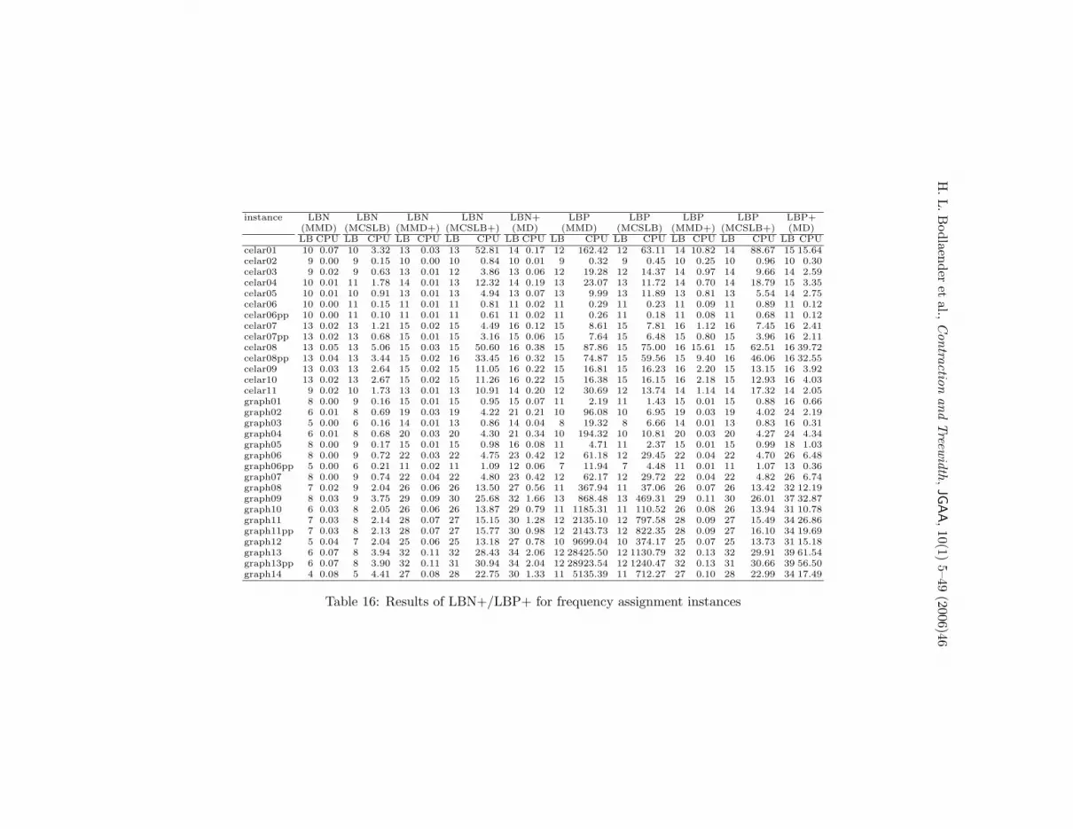
H.L.B
odlaen
der
etal.,
Contra
ction
and
Treew
idth
,JG
AA
,10(1)
5–49(2006)46
instance LBN LBN LBN LBN LBN+ LBP LBP LBP LBP LBP+(MMD) (MCSLB) (MMD+) (MCSLB+) (MD) (MMD) (MCSLB) (MMD+) (MCSLB+) (MD)LB CPU LB CPU LB CPU LB CPU LB CPU LB CPU LB CPU LB CPU LB CPU LB CPU
celar01 10 0.07 10 3.32 13 0.03 13 52.81 14 0.17 12 162.42 12 63.11 14 10.82 14 88.67 15 15.64celar02 9 0.00 9 0.15 10 0.00 10 0.84 10 0.01 9 0.32 9 0.45 10 0.25 10 0.96 10 0.30celar03 9 0.02 9 0.63 13 0.01 12 3.86 13 0.06 12 19.28 12 14.37 14 0.97 14 9.66 14 2.59celar04 10 0.01 11 1.78 14 0.01 13 12.32 14 0.19 13 23.07 13 11.72 14 0.70 14 18.79 15 3.35celar05 10 0.01 10 0.91 13 0.01 13 4.94 13 0.07 13 9.99 13 11.89 13 0.81 13 5.54 14 2.75celar06 10 0.00 11 0.15 11 0.01 11 0.81 11 0.02 11 0.29 11 0.23 11 0.09 11 0.89 11 0.12celar06pp 10 0.00 11 0.10 11 0.01 11 0.61 11 0.02 11 0.26 11 0.18 11 0.08 11 0.68 11 0.12celar07 13 0.02 13 1.21 15 0.02 15 4.49 16 0.12 15 8.61 15 7.81 16 1.12 16 7.45 16 2.41celar07pp 13 0.02 13 0.68 15 0.01 15 3.16 15 0.06 15 7.64 15 6.48 15 0.80 15 3.96 16 2.11celar08 13 0.05 13 5.06 15 0.03 15 50.60 16 0.38 15 87.86 15 75.00 16 15.61 15 62.51 16 39.72celar08pp 13 0.04 13 3.44 15 0.02 16 33.45 16 0.32 15 74.87 15 59.56 15 9.40 16 46.06 16 32.55celar09 13 0.03 13 2.64 15 0.02 15 11.05 16 0.22 15 16.81 15 16.23 16 2.20 15 13.15 16 3.92celar10 13 0.02 13 2.67 15 0.02 15 11.26 16 0.22 15 16.38 15 16.15 16 2.18 15 12.93 16 4.03celar11 9 0.02 10 1.73 13 0.01 13 10.91 14 0.20 12 30.69 12 13.74 14 1.14 14 17.32 14 2.05graph01 8 0.00 9 0.16 15 0.01 15 0.95 15 0.07 11 2.19 11 1.43 15 0.01 15 0.88 16 0.66graph02 6 0.01 8 0.69 19 0.03 19 4.22 21 0.21 10 96.08 10 6.95 19 0.03 19 4.02 24 2.19graph03 5 0.00 6 0.16 14 0.01 13 0.86 14 0.04 8 19.32 8 6.66 14 0.01 13 0.83 16 0.31graph04 6 0.01 8 0.68 20 0.03 20 4.30 21 0.34 10 194.32 10 10.81 20 0.03 20 4.27 24 4.34graph05 8 0.00 9 0.17 15 0.01 15 0.98 16 0.08 11 4.71 11 2.37 15 0.01 15 0.99 18 1.03graph06 8 0.00 9 0.72 22 0.03 22 4.75 23 0.42 12 61.18 12 29.45 22 0.04 22 4.70 26 6.48graph06pp 5 0.00 6 0.21 11 0.02 11 1.09 12 0.06 7 11.94 7 4.48 11 0.01 11 1.07 13 0.36graph07 8 0.00 9 0.74 22 0.04 22 4.80 23 0.42 12 62.17 12 29.72 22 0.04 22 4.82 26 6.74graph08 7 0.02 9 2.04 26 0.06 26 13.50 27 0.56 11 367.94 11 37.06 26 0.07 26 13.42 32 12.19graph09 8 0.03 9 3.75 29 0.09 30 25.68 32 1.66 13 868.48 13 469.31 29 0.11 30 26.01 37 32.87graph10 6 0.03 8 2.05 26 0.06 26 13.87 29 0.79 11 1185.31 11 110.52 26 0.08 26 13.94 31 10.78graph11 7 0.03 8 2.14 28 0.07 27 15.15 30 1.28 12 2135.10 12 797.58 28 0.09 27 15.49 34 26.86graph11pp 7 0.03 8 2.13 28 0.07 27 15.77 30 0.98 12 2143.73 12 822.35 28 0.09 27 16.10 34 19.69graph12 5 0.04 7 2.04 25 0.06 25 13.18 27 0.78 10 9699.04 10 374.17 25 0.07 25 13.73 31 15.18graph13 6 0.07 8 3.94 32 0.11 32 28.43 34 2.06 12 28425.50 12 1130.79 32 0.13 32 29.91 39 61.54graph13pp 6 0.07 8 3.90 32 0.11 31 30.94 34 2.04 12 28923.54 12 1240.47 32 0.13 31 30.66 39 56.50graph14 4 0.08 5 4.41 27 0.08 28 22.75 30 1.33 11 5135.39 11 712.27 27 0.10 28 22.99 34 17.49
Table 16: Results of LBN+/LBP+ for frequency assignment instances

H.L.B
odlaen
der
etal.,
Contra
ction
and
Treew
idth
,JG
AA
,10(1)
5–49(2006)47
instance LBN LBN LBN LBN LBN+ LBP LBP LBP LBP LBP+(MMD) (MCSLB) (MMD+) (MCSLB+) (MD) (MMD) (MCSLB) (MMD+) (MCSLB+) (MD)LB CPU LB CPU LB CPU LB CPU LB CPU LB CPU LB CPU LB CPU LB CPU LB CPU
celar01-pp 10 0.04 10 0.43 13 0.02 13 2.84 14 0.06 13 55.96 13 21.25 14 3.89 14 8.31 15 8.87celar02-pp 10 0.00 10 0.00 10 0.01 10 0.02 10 0.00 10 0.03 10 0.03 10 0.02 10 0.04 10 0.02celar03-pp 10 0.01 10 0.11 13 0.00 13 0.74 13 0.02 12 3.38 12 2.00 14 0.28 13 0.93 14 0.90celar04-pp 10 0.01 11 0.24 13 0.02 13 1.47 14 0.07 13 5.97 13 2.75 14 0.44 14 2.51 15 1.57celar05-pp 10 0.01 10 0.16 13 0.01 12 0.74 13 0.02 13 4.49 13 4.82 13 0.34 13 1.98 14 1.52celar07-pp 13 0.01 13 0.25 15 0.01 15 1.08 16 0.05 15 3.90 15 3.24 16 0.40 16 1.95 16 0.90celar08-pp 13 0.02 13 1.00 15 0.01 15 4.66 16 0.15 15 33.64 15 35.31 15 6.73 16 22.61 16 23.85celar09-pp 13 0.02 13 0.45 15 0.02 15 2.07 16 0.09 15 7.09 15 8.27 15 0.86 16 5.86 16 1.54celar10-pp 13 0.02 13 0.47 15 0.01 15 1.99 16 0.09 15 9.78 15 8.27 15 0.89 16 4.61 16 1.42celar11-pp 10 0.01 10 0.16 13 0.00 13 0.94 14 0.06 12 8.27 12 4.96 14 0.39 14 1.76 14 1.13graph01-pp 8 0.00 9 0.14 14 0.01 15 0.72 15 0.03 11 1.42 11 1.25 14 0.02 15 1.30 16 0.26graph02-pp 6 0.01 8 0.53 19 0.03 19 3.33 21 0.21 10 38.95 10 8.55 19 0.06 19 5.27 24 1.99graph03-pp 6 0.00 6 0.10 14 0.01 14 0.57 14 0.07 10 3.67 10 3.84 14 0.02 14 0.92 16 0.47graph04-pp 6 0.01 8 0.55 20 0.03 20 3.44 21 0.32 11 82.46 11 11.29 20 0.05 20 5.84 24 4.22graph05-pp 8 0.00 9 0.14 15 0.01 15 0.85 16 0.08 11 6.26 11 3.07 15 0.02 15 1.46 18 0.80graph06-pp 8 0.01 9 0.58 22 0.03 22 4.08 23 0.39 12 50.71 12 28.18 22 0.05 22 5.81 26 6.40graph07-pp 8 0.01 9 0.61 22 0.03 22 4.03 23 0.40 12 50.35 12 26.60 22 0.04 22 5.52 26 6.36graph08-pp 7 0.01 8 2.53 26 0.10 26 13.80 27 0.53 12 194.21 12 73.90 26 0.09 26 15.62 32 11.73graph09-pp 8 0.02 9 3.56 29 0.08 29 22.77 31 1.18 13 220.09 13 162.56 29 0.19 29 35.83 37 33.81graph10-pp 6 0.02 8 1.92 26 0.06 26 13.55 29 1.08 11 684.95 11 94.07 26 0.07 26 13.28 31 16.21graph11-pp 7 0.03 9 1.77 28 0.07 27 13.75 30 0.90 13 569.82 13 73.34 28 0.08 27 13.11 34 20.72graph12-pp 6 0.02 7 1.85 25 0.06 25 11.70 27 0.76 11 528.67 11 114.95 25 0.08 25 11.73 31 15.34graph13-pp 6 0.07 8 3.54 32 0.10 32 25.62 34 2.01 13 3186.53 13 344.59 32 0.12 32 26.96 39 62.66graph14-pp 5 0.03 6 2.75 27 0.06 28 17.38 30 1.25 13 198.29 13 106.43 27 0.10 28 17.59 34 16.91
Table 17: Results of LBN+/LBP+ for preprocessed versions of frequency assignment instances

H.L.B
odlaen
der
etal.,
Contra
ction
and
Treew
idth
,JG
AA
,10(1)
5–49(2006)48
instance LBN LBN LBN LBN LBN+ LBP LBP LBP LBP LBP+(MMD) (MCSLB) (MMD+) (MCSLB+) (MD) (MMD) (MCSLB) (MMD+) (MCSLB+) (MD)LB CPU LB CPU LB CPU LB CPU LB CPU LB CPU LB CPU LB CPU LB CPU LB CPU
fl3795 3 0.42 4 66.52 6 0.12 6 352.62 3 0.73 - - - - 6 65.26 6 415.54 - -fnl4461 3 0.40 4 169.78 5 0.20 5 882.32 3 0.91 - - - - 6 9.76 6 1317.62 - -pcb3038 3 0.83 4 57.82 5 0.11 5 282.95 3 3.39 - - - - 5 1.53 5 272.68 - -rl5915 3 0.17 4 53.56 5 0.11 5 252.75 3 0.70 - - - - 6 9.05 6 385.44 - -rl5934 3 0.18 4 60.28 5 0.11 5 285.51 3 0.69 - - - - 6 5.45 6 429.39 - -
fl3795-pp 3 0.36 4 31.06 6 0.10 6 163.79 3 1.32 - - - - 6 40.66 6 215.22 7 4269.18fnl4461-pp 3 0.36 4 36.51 5 0.10 5 180.71 3 0.70 - - - - 6 79.71 6 413.34 - -pcb3038-pp 3 0.15 4 13.50 5 0.06 5 62.74 3 0.30 - - - - 6 10.43 6 107.43 8 34030.60rl5915-pp 3 0.14 4 10.96 5 0.05 5 53.00 3 0.31 - - - - 6 7.32 6 89.13 9 54819.50rl5934-pp 3 0.14 4 11.93 5 0.05 6 61.69 3 0.55 - - - - 6 5.86 6 56.51 9 38137.20
Table 18: Results of LBN+/LBP+ for TSP graphs and preprocessed versions of these

H.L.B
odlaen
der
etal.,
Contra
ction
and
Treew
idth
,JG
AA
,10(1)
5–49(2006)49
instance LBN LBN LBN LBN LBN+ LBP LBP LBP LBP LBP+(MMD) (MCSLB) (MMD+) (MCSLB+) (MD) (MMD) (MCSLB) (MMD+) (MCSLB+) (MD)
LB CPU LB CPU LB CPU LB CPU LB CPU LB CPU LB CPU LB CPU LB CPU LB CPUanna 10 0.00 10 0.28 11 0.00 12 1.88 12 0.22 11 1.03 11 1.44 12 0.74 12 2.26 12 1.67david 10 0.01 10 0.12 12 0.01 12 0.87 12 0.06 11 0.98 11 1.13 12 0.36 12 1.23 12 0.61fpsol2.i.1 66 0.23 66 4.91 66 0.25 66 93.64 66 5.03 66 1402.59 66 656.75 66 656.36 66 752.30 66 1810.12games120 8 0.00 10 0.27 19 0.02 20 1.98 21 0.36 12 88.04 12 12.85 19 0.02 20 1.99 24 2.48homer 14 0.08 14 6.38 23 0.03 23 52.19 25 3.12 21 94.01 21 93.80 24 7.44 24 87.00 26 88.39huck 10 0.00 10 0.09 10 0.00 10 0.69 10 0.04 10 0.03 10 0.11 10 0.03 10 0.69 10 0.10inithx.i.1 56 0.43 56 16.68 56 0.47 56 326.61 56 14.75 56 7085.94 56 5588.02 56 5688.78 56 6032.99 56 3937.69jean 9 0.00 9 0.08 9 0.01 9 0.49 9 0.04 9 0.36 9 0.44 9 0.36 9 0.85 9 0.67le450-15a 24 0.32 28 8.31 73 0.53 74 145.57 80 48.59 56 8613.52 56 11511.59 73 17.78 74 170.65 94 33607.00le450-15c 49 1.02 51 14.57 110 1.31 110 283.65 118 196.08 92 41950.71 92 53453.79 110 194.46 110 487.54 139 301507.92le450-25a 27 0.68 30 8.04 75 0.49 75 148.21 81 40.36 62 7227.17 62 8449.98 77 209.07 77 515.26 96 29270.39le450-25c 52 0.93 55 14.34 111 1.31 111 290.95 121 228.82 100 36727.37 100 45282.66 116 1453.15 116 2527.20 144 818568.19le450-5a 17 0.27 20 7.85 62 0.39 63 100.06 66 17.13 33 6955.30 33 6207.72 62 0.42 63 100.46 79 6149.43le450-5c 33 0.62 35 10.14 86 0.78 86 173.22 93 48.27 51 19667.36 51 21950.36 86 0.73 86 168.45 106 30076.05miles1000 44 0.27 46 0.81 48 0.07 48 11.43 49 1.01 47 245.14 47 125.33 49 113.87 49 129.82 49 337.91miles1500 76 0.20 76 2.58 77 0.11 77 14.82 77 0.63 76 399.24 76 275.38 77 107.52 77 122.32 77 113.30miles250 8 0.00 8 0.22 9 0.01 9 2.28 9 0.07 8 2.48 8 1.29 9 0.64 9 2.86 9 0.78miles500 21 0.03 22 0.60 22 0.02 22 4.36 22 0.16 22 21.88 22 11.70 22 6.56 22 10.93 22 14.52miles750 32 0.03 32 0.57 34 0.04 34 7.70 34 0.35 33 70.08 34 64.44 34 27.06 34 35.66 35 160.10mulsol.i.1 50 0.10 50 0.96 50 0.08 50 13.22 50 0.75 50 243.02 50 120.56 50 118.76 50 135.98 50 103.11mulsol.i.2 32 0.07 32 1.21 32 0.07 32 17.29 32 1.10 32 111.41 32 73.47 32 73.49 32 91.28 32 68.10myciel3 3 0.00 3 0.00 4 0.00 4 0.00 5 0.00 4 0.00 4 0.00 4 0.00 4 0.01 5 0.00myciel4 5 0.00 5 0.00 8 0.01 8 0.03 8 0.01 6 0.02 6 0.03 8 0.00 8 0.04 9 0.01myciel5 8 0.00 8 0.04 14 0.00 14 0.24 15 0.07 12 0.33 12 0.44 14 0.04 15 0.40 16 0.25myciel6 15 0.21 15 0.53 24 0.02 25 1.93 27 0.26 20 5.02 20 4.77 26 0.26 26 2.98 29 1.94myciel7 25 2.96 25 6.45 43 0.08 44 23.61 46 3.39 34 88.09 34 76.75 44 7.65 45 36.74 52 174.52queen12-12 33 0.02 33 0.83 43 0.09 44 9.18 44 0.78 37 101.99 38 114.91 43 0.08 44 8.85 55 363.91queen15-15 42 0.08 42 2.37 58 0.24 59 32.85 60 7.36 48 1045.63 50 1221.13 58 0.24 59 32.01 73 7579.01queen16-16 45 0.12 45 3.33 63 0.31 64 46.89 66 13.44 53 2005.27 53 2512.97 63 0.31 64 46.05 79 16312.83queen5-5 12 0.00 12 0.01 12 0.00 12 0.06 12 0.01 12 0.00 12 0.03 13 0.01 13 0.09 14 0.04queen6-6 15 0.00 15 0.03 15 0.01 15 0.18 16 0.05 15 0.08 16 0.13 17 0.09 17 0.41 18 0.35queen8-12 25 0.02 25 0.35 33 0.04 34 2.96 34 0.46 30 23.52 30 28.56 33 0.04 34 2.66 39 19.54queen9-9 24 0.01 24 0.19 30 0.03 30 1.61 30 0.31 26 5.46 26 5.93 30 0.03 30 1.60 35 9.75school1 88 375.93 88 156.33 122 1.49 122 347.09 132 180.80 116 65019.15 116 66247.57 128 3668.42 127 4722.53 149 207254.65school1-nsh 72 198.00 72 11.47 106 0.90 108 219.47 116 112.63 100 51399.36 100 45639.51 111 1801.06 112 2066.21 132 139781.41zeroin.i.1 50 0.06 50 0.85 50 0.08 50 10.23 50 0.78 50 72.33 50 36.11 50 35.21 50 45.28 50 33.40zeroin.i.2 31 0.20 31 1.03 32 0.07 32 12.81 32 1.05 31 211.19 31 72.98 32 57.15 32 69.75 32 74.14
Table 19: Results of LBN+/LBP+ for some DIMACS colouring instances


