Copyright and use of this thesis - University of Sydney

Copyright and use of this thesis

This thesis must be used in accordance with the provisions of the Copyright Act 1968.

Reproduction of material protected by copyright may be an infringement of copyright and copyright owners may be entitled to take legal action against persons who infringe their copyright.

Section 51 (2) of the Copyright Act permits an authorized officer of a university library or archives to provide a copy (by communication or otherwise) of an unpublished thesis kept in the library or archives, to a person who satisfies the authorized officer that he or she requires the reproduction for the purposes of research or study.

The Copyright Act grants the creator of a work a number of moral rights, specifically the right of attribution, the right against false attribution and the right of integrity.

You may infringe the author’s moral rights if you:

- fail to acknowledge the author of this thesis if you quote sections from the work

- attribute this thesis to another author

- subject this thesis to derogatory treatment which may prejudice the author’s reputation

For further information contact the University’s Director of Copyright Services

sydney.edu.au/copyright

Studies in relativity and quantuminformation theory

Maki Takahashi

A thesis submitted in fulfilment of the requirementsfor the degree of

Doctor of Philosophy

The University of SydneyFaculty of ScienceSchool of Physics

December 2013

mailto:[email protected]

i

c© Maki Takahashi, 2013.

Typeset in LATEX 2ε.

mailto:[email protected]

ii

“they tell me you have written this large book on the system of the universe, and havenever even mentioned its Creator”

Napoleon Bonaparte

“I had no need of that hypothesis.”Pierre-Simon Laplace

iii

Abstract

The current foundations of theoretical physics can be summarised by the two corner-stones of physics, namely quantum mechanics and relativity theory. One can probablyadd to this list information theory since as observers we are in essence informationgatherers from which one deduces certain aspects of these theories as well as makingpredictions. In this thesis we will explore various aspects of these theories as well asthe interactions between them. This thesis can be broken into three broad topics whichfit into and overlap various aspects of these three cornerstones of physics.

The main topic of this thesis is on relativistic quantum information theory. Here weconstruct a reformulation of quantum information which is consistent with relativitytheory. We will see that by providing a rigorous formulation starting with the fieldequations for a massive fermion and a photon we can construct a theory for relativisticquantum information. In particular we provide a measurement formalism, a transportequation which describes the unitary evolution of a state through spacetime as well ashow to extend this to multipartite systems.

The second topic concerns the nature of time, duration and clocks in current phys-ical theories and in particular for Newtonian mechanics. We analyse the relationshipbetween the readings of clocks in Newtonian mechanics with absolute time. We will seethat in order to answer this question we must provide not only a model for a clock butalso solve what is referred to as Newton’s Scholium problem. We then compare thiswith other dynamical theories in particular quantum mechanics and general relativitywhere the treatment of time is quite different from Newtonian mechanics.

The final topic is rather different from the first two. In this chapter we investigatea range of methods to perform tomography in a solid-state qubit device, for which apriori initialization and measurement of the qubit is restricted to a single basis of theBloch sphere. We explore and compare several methods to acquire precise descriptionsof additional states and measurements, quantifying both stochastic and systematicerrors, ultimately leading to a tomographically-complete set that can be subsequentlyused in process tomography. We focus in detail on the example of a spin qubit formedby the singlet-triplet subspace of two electron spins in a GaAs double quantum dot,although our approach is quite general.

These three parts are followed by a personal (and possibly controversial) conclusion,which describes my fascination with, and ultimately my reason for pursuing studies inrelativity, quantum information and the foundations of physics.

iv

Statement of Students Contribution

Except where acknowledged in the customary manner,the material presented in this thesis is, to the best of myknowledge, original and has not been submitted in wholeor part for a degree in any university.

Maki Takahashi

v

Publications and Attributions

Relativistic Quantum Information

1. Matthew C. Palmer, Maki Takahashi and Hans F. Westman, Localized qubits incurved spacetimes. Annals Phys. 327 (2012) 1078-1131.

2. Matthew C. Palmer, Maki Takahashi and Hans F. Westman, WKB analysis ofrelativistic Stern-Gerlach measurements. Annals Phys. 336 (2013) 505516.

This is a comprehensive body of work which was developed in collaboration with Dr.Hans F. Westman and Mr Matthew C. Palmer. The initial idea of the project wasproposed by HW. The research and production of these two publications has beenequally divided amongst MP, HW and myself. There are however, particular resultsfor which there is ownership. Furthermore due to restrictions in publication lengththere are additional results which have been included in this thesis which were notincluded in the final publications. They are as follows:

Ch.4 MP and HW were responsible for the research in section 4.2, I contributed todiscussions and the writing of this section. The results presented in sections 4.3.4,4.4.4 and 4.4.5 are entirely my work. Sections 4.4.4 and 4.4.5 contains entirelynew material not found in (1). The material is mathematically distinct butempirically equivalent to that in (1). For the purpose of comparison the originalmaterial is included in Appendix A, the results contained in the appendix wasprimarily the work of MP. The formalism presented in sections 4.4.4 and 4.4.5impact various additional results presented in later sections and they have beenmodified to reflect these results.

Ch.5 Section 5.4 is new material which is entirely my work, and identifies additionalgeometric phases which have not been considered in (1). The numerical calcula-tions at the end of Section 5.5 is the work of MP.

Ch.6 This research for this chapter has been shared amongst the three of us and thereare no notable attributions to be made.

Ch.7 This chapter is entirely based on publication (2). The initial idea can be at-tributed to MP. I have made a significant contribution to the research for thisproject and in particular towards the key result of this paper Section 7.3. Thisderivation of the relativistic spin measurement is the work of MP and myself, andhas been independently checked by HW. MP and myself are responsible for the

vi

http://www.sciencedirect.com/science/article/pii/S0003491611001692

http://www.sciencedirect.com/science/article/pii/S0003491613001279

vii

writing of this publication. Section 7.4 is new material not included in (2) andis entirely my work.

The Newton Scholium Problem

Maki Takahashi, Dean Rickles and Hans F. Westman, Not all together desperate: theNewton Scholium Problem. In preparation.

The initial idea for this research project was proposed by Dr. Hans F. Westman.The research was collaborative with Dr. Dean Rickles, HW and myself contributingequally to the historical and philosophical research. HW and myself were responsiblefor the mathematical research. I played a central role in developing the mathematicalformulation, carrying out the calculations and investigating possible solutions of thisproblem. I am primarily responsible for the writing of this paper.

Tomography of a spin qubit

Maki Takahashi, Stephen Bartlett and Andrew Doherty, Tomography of a spin qubitin a double quantum dot. Phys. Rev. A 88, 022120 (2013).

This initial idea for this research project was proposed by Prof. Stephen Bartlettand A. Prof. Andrew Doherty. I was responsible for the research and in particular forall the calculations, the development of numerical code and simulations. I am primarilyresponsible for the writing of this paper.

http://pra.aps.org/abstract/PRA/v88/i2/e022120

Acknowledgements

I would like to thank my supervisor, Dr Hans Westman for his support and encour-agement, for being patient with my never ending list of questions and finally for hiswisdom which has assisted beyond measure, my journey in becoming a researcher. Iwould also like to thank Prof. Stephen Bartlett for his guidance throughout the courseof my PhD. During my PhD, I have enjoyed many discussions with fellow physicists.In particular I would like to thank Andrew Doherty, Danny Terno, Dean Rickles, NickMenicucci, Aharon Brodutch, Nikolai Friss and Florian Girelli.

I would like to thank the University of Sydney and the School of Physics for sup-porting me both financially and for providing me with an environment conducive toresearch. I would also like to thank the Perimeter Institute for Theoretical Physicsfor providing funding to visit for three weeks which assisted me in developing as aresearcher.

I would like to thank my colleague Dr Matthew Palmer for being available to discussmy many stupid ideas. I would like to thank my friends Andrew D., Andrew L., Brett,Courtney, Jacob, Joel, Matt and Raph for being helpful distractions from my research.I am also grateful to My house mates for not believing that this day would come.

I am thankful to my parents for their, encouragement and support throughout mylife and to my mother-in-law Sharon for her loving support. Finally I am grateful tomy loving partner, Emma, for enduring my endless doubts, questions, ramblings andso forth throughout the years with incredible patience.

viii

Author’s Note

In writing this thesis there were several choices regarding the style and format thatI would like to note. Firstly I would like to point out what this thesis is not: This thesisis not intended to convey a coherent story, research indeed is not like that rather asscientists we identify areas where we believe progress can be made. Only after decadeseven centuries when we step back do we begin to see the bigger picture. This thesisis simply a collection of research projects both large and small varying over variousdifferent fields some leaning towards philosophy others couched in experiments. Theseare areas which not only interested me but where I believed answers can be found fromdeep problems regarding the quantization of gravity to answering the simple question“what is my state?” or “what gate did I just perform?”.

In this light let us address the first issue regarding the basic format of the thesis,that is whether to present a traditional thesis or simply a ‘thesis by publication’. HereI have opted to present my research somewhere in between these two formats: thoseprojects which are small self contained bodies of work I have simply presented thepapers in essentially the same way as they were or will be published. Others are muchlarger and I have here for the readers sanity avoided repetition and presented a moretraditional format which we might call a thesis.

In particular the first part is in the field of relativistic quantum information whichhas been the primary field of research during my PhD. In this part of the thesis Ihave adopted a traditional thesis format. There are several reasons for this: firstly inorder to avoid repetition a traditional thesis seemed more suitable. Secondly, duringthe preparation of each paper there were several decisions to remove some resultsfor not being inline with the primary focus of each paper which were perhaps bettersuited to a thesis style document. As these represented a significant research efforton my part I have decided to include them and I have indicated in the Publicationsand Attributions section where such results have been included. Having said this themajority of the chapters have been left untouched from the original manuscripts. Incontrast the second part of this thesis represents several fields of research with smallresearch projects. As these projects are small self contained bodies of work I havepresented these ‘by publication’.

In regards to the use of pronouns, since the majority of the work is research thatwas collaborative in nature I will use ‘we’ rather than ‘I’ throughout for consistency,unless I am conveying an opinion not shared by my collaborators. I hope you enjoyreading this at least as much as I did writing it.

ix

x Author’s Note

Contents

Abstract iv

Statement of Students Contribution v

Publications and Attributions vi

Acknowledgements viii

Author’s Note ix

List of Figures xv

List of Symbols xviii

1 Introduction 11.1 Outline of the Thesis . . . . . . . . . . . . . . . . . . . . . . . . . . . . 2

I Relativistic Quantum Information 5

2 Introduction to RQI 7

3 Preliminaries Localized qubits in curved spacetimes 113.1 Mathematical tools . . . . . . . . . . . . . . . . . . . . . . . . . . . . . 113.2 Relativistic Quantum Information circa 2009 . . . . . . . . . . . . . . . 183.3 Relativistic quantum information . . . . . . . . . . . . . . . . . . . . . 22

4 Relativistic qubits 254.1 An outline of methods and concepts . . . . . . . . . . . . . . . . . . . . 254.2 Issues from quantum field theory - the domain of applicability . . . . . 294.3 The qubit as the spin of a massive fermion . . . . . . . . . . . . . . . . 334.4 The qubit as the polarization of a photon . . . . . . . . . . . . . . . . . 44

5 Phases and interferometry 555.1 Spacetime Mach–Zehnder interferometry . . . . . . . . . . . . . . . . . 565.2 The phase difference from the WKB approximation . . . . . . . . . . . 575.3 The physical interpretation of phase in terms of wave geometry . . . . 61

xi

xii Contents

5.4 Geometric phase . . . . . . . . . . . . . . . . . . . . . . . . . . . . . . 64

5.5 An example: relativistic neutron interferometry . . . . . . . . . . . . . 66

6 Relativistically covariant quantum information 71

6.1 Elementary operations and measurement formalism . . . . . . . . . . . 71

6.2 Quantum entanglement . . . . . . . . . . . . . . . . . . . . . . . . . . . 77

7 Relativistic Stern-Gerlach measurements 83

7.1 Hermitian operators and spin observables . . . . . . . . . . . . . . . . . 84

7.2 Intuitive derivation of the Stern-Gerlach observable . . . . . . . . . . . 84

7.3 WKB analysis of a Stern-Gerlach measurement . . . . . . . . . . . . . 86

7.4 Comparison of spin operators . . . . . . . . . . . . . . . . . . . . . . . 90

7.5 Summary . . . . . . . . . . . . . . . . . . . . . . . . . . . . . . . . . . 95

8 Conclusion 97

II 103

9 “Not all together desperate” - the Newton Scholium Problem 105

9.1 Theory of clocks and their accuracy . . . . . . . . . . . . . . . . . . . . 107

9.2 Newton’s Scholium . . . . . . . . . . . . . . . . . . . . . . . . . . . . . 111

9.3 A ‘modern take’ on the Newton Scholium . . . . . . . . . . . . . . . . . 112

9.4 Solving the Scholium Problem: What does it take? . . . . . . . . . . . 116

9.5 Modern Clocks . . . . . . . . . . . . . . . . . . . . . . . . . . . . . . . 118

9.6 Time and duration in different dynamical theories . . . . . . . . . . . . 119

9.7 Conclusion . . . . . . . . . . . . . . . . . . . . . . . . . . . . . . . . . . 122

10 Tomography of a spin qubit in a double quantum dot 125

10.1 Introduction . . . . . . . . . . . . . . . . . . . . . . . . . . . . . . . . . 125

10.2 Spin singlet-triplet qubits . . . . . . . . . . . . . . . . . . . . . . . . . 127

10.3 Tomography for states and measurements . . . . . . . . . . . . . . . . . 130

10.4 Process tomography . . . . . . . . . . . . . . . . . . . . . . . . . . . . 138

10.5 Conclusion . . . . . . . . . . . . . . . . . . . . . . . . . . . . . . . . . . 140

III Conclusion and Outlook 143

11 The future of relativistic quantum information theory 145

A The original qubit formalism 149

A.1 The quantum state . . . . . . . . . . . . . . . . . . . . . . . . . . . . . 149

A.2 The inner product . . . . . . . . . . . . . . . . . . . . . . . . . . . . . 152

A.3 The relation to the Wigner formalism . . . . . . . . . . . . . . . . . . . 152

Contents xiii

B Null Fermi-Walker transport 155B.1 Jerk and non-geodesic motion . . . . . . . . . . . . . . . . . . . . . . . 155

C Relationship between Wigner and Weyl representations 157C.1 Relation to the Wigner representation . . . . . . . . . . . . . . . . . . . 158

References 161

xiv Contents

List of Figures

4.1 The comparison between tangent spaces and Hilbert spaces on a curvedspacetime manifold. . . . . . . . . . . . . . . . . . . . . . . . . . . . . . 26

5.1 A spacetime picture of a Mach-Zehnder type interference experiment. . 57

5.2 An illustration of depicting the accumulation of internal phase. . . . . . 62

5.3 An illustration of displacement phase. . . . . . . . . . . . . . . . . . . . 63

5.4 An illustration of internal and displacement phase. . . . . . . . . . . . 64

5.5 A Schematic diagram of a Neutron interferometer used in the COWexperiment. . . . . . . . . . . . . . . . . . . . . . . . . . . . . . . . . . 66

7.1 Comparison of expectation values for three distinct relativistic spin op-erators. . . . . . . . . . . . . . . . . . . . . . . . . . . . . . . . . . . . . 94

10.1 The Bloch sphere is defined at the point labelled εBS, where we haveplotted the energy levels as a function of ε the gate voltage. The z-basiscorresponds to the energy eigenstates of the Hamiltonian at the pointεBS. . . . . . . . . . . . . . . . . . . . . . . . . . . . . . . . . . . . . . 128

10.2 Schematic illustration of the ε pulse sequence for the z preparation andmeasurement as a function of time t. The pulse starts at the measure-ment point εM and rapidly but adiabatically ramps down to the qubitpoint εBS. See Ref. [140] for details. . . . . . . . . . . . . . . . . . . . . 132

10.3 Schematic illustration of the pulse sequence for the (a) +x and (b) +ypreparation and measurement. . . . . . . . . . . . . . . . . . . . . . . . 133

10.4 Comparison of state and measurement reconstruction for method A(green), B (blue) and C (red). (a) The convergence of a systematicerror for the measurement Ex. Here, α is the angular separation be-tween the vector R2

i and the true measurement with respect to the totalnumber of measurements N . (b) The infidelity 1− F between the truestate ρ1 and reconstructed state ρest1 . The data has been averaged over10 runs per point in order to highlight the difference in average-caseperformance of Methods B and C. . . . . . . . . . . . . . . . . . . . . 138

xv

xvi List of Figures

10.5 Process fidelities for the Hadamard gate, reconstructed using states andmeasurements characterised from method A (green), B (blue), and C(red). (a),(b) the infidelity between the ideal unitary ρU and the re-constructed process ρEest based on state and measurement tomographyobtained for NSPAM = 106 (a) and NSPAM = 109 (b) total measurementsrespectively. The solid line represents the fidelity between the true pro-cess and the ideal Hadamard gate; process tomography estimates shouldconverge to this line. (c),(d) the fidelity between the true E and recon-structed process Eest, again for NSPAM = 106 (c) and NSPAM = 109 (d)total measurements respectively. These process tomography estimatesshould improve continuously as 1/

√N . The data has been averaged over

10 runs per point. . . . . . . . . . . . . . . . . . . . . . . . . . . . . . . 141

A.1 Adaption of tetrad . . . . . . . . . . . . . . . . . . . . . . . . . . . . . 151

C.1 Comparison between the action of a Lorentz transformation on spindegrees of freedom for Weyl and Wigner representations. . . . . . . . . 160

List of Symbols

α, β, γ, δ, . . . denotes flat spacetime tensor indices

µ, ν, ρ, σ, . . . denotes curved spacetime tensor indices

I, J,K, L, . . . = 0, 1, 2, 3 denotes spacetime tetrad indices

i, j, k, l, . . . = 1, 2, 3 denotes spatial components of tetrad indices

A,B,C,D, . . . = 1, 2 denotes spinor indices when working with fermions or diad indiceswhen working with photons.

A′, B′, C ′, D′, . . . = 1, 2 denotes conjugate spinor indices. The diad indices do not haveconjugate indices.

eµI (x) The tetrad field

eµA The diad field, where A is a diad index

gµν The spacetime metric

hµν Denotes the projector onto the space orthogonal to some time-like or light-like4-velocity uµ.

ηIJ = diag(1,−1,−1,−1) The locally falt Minkowski metric

δAB Local metric on the two dimensional space orthogonal the photons 4-velocityuµ, where A,B are diad indices

Γµνρ The affine connection

ω Iν J The spin-1 connection, or connection 1-form

WµAB Connection on the space orthognal to the photons four-velcoity uµ, where A,B

are diad indices

(LIJ) BA and (RIJ)A

′

B′ The left- and right-handed generators of SL(2,C)

ΛIJ An arbitrary Lorentz transformation

|p, σ〉 A momentum eignenstate in the Wigner representation

xvii

xviii List of Figures

Hx,p The Hilbert space for a relativistic qubit, where x and p labels the position andmomentum

ψA Tilde ∼ denotes quantities evaluated in the qubits rest frame

IA′A The inner product structure for spinors

1Introduction

Over the past 80 years there has been an enormous research effort into the field ofQuantum Gravity [1–4] the primary aim being to construct a quantum theory of grav-ity which should in principle answer or at the very least shed light on the very peculiarfeatures encountered at the boundary of quantum theory and gravitational physics,such as the black hole information paradox, Hawking radiation and much more [5, 6].Unfortunately, this research field has been long and arduous with very few significantbreakthroughs. Much of the difficulty has been due to a lack of any clear experimentalindication as to how one should proceed in quantizing gravity as well as many technicalchallenges faced when applying the standard quantization tools that have proved souseful in quantizing virtually any other gauge theory. In contrast, more recently therehas been an enormous amount of progress in quantum information theory and quantumcomputation and although the long term goal of developing a quantum computer hasbeen highly elusive, one can not deny that the field has evolved into an empirically pre-cise science. In this thesis we would like to explore from a theoretical perspective howone might gain some insight into the field of quantum gravity, our approach howeverwill not be concerned with the difficult task of quantizing gravity but rather asking themuch simpler question of what we can learn about gravity from quantum theory andmore specifically quantum information theory.

Before we embark on such a journey it is reasonable to ask why we think thisis the right question and what do we think we would gain? The answer to this ishistorical: since the discovery of special relativity in 1905, it was well known to thephysics community that the (at the time) highly successful and accurate theory ofNewtonian gravity was not consistent with special relativity and the question was howto ‘relativize gravity’ so that it is consistent with special relativity. While there hadbeen many attempts to do this, Einstein and (perhaps less well known) Hilbert werethe first to construct such a theory[7, 8]. Einstein’s approach to constructing his theoryhinged on

1

2 Introduction

1. The geometrical formulation of special relativity developed by Minkowski, wherethe three dimensional ‘ether’ is replaced by the four dimensional spacetime.

2. Asking the operational question: what can be learned by probing gravity usingclassical test particles? Following such a thought process Einstein concluded thatthe aspect of Newtonian gravity that should be retained is the equivalence prin-ciple. The most widely accepted version of this principle is the strong equivalenceprinciple according to which in an Einstein elevator that is freely falling, the lawsof special relativity are approximately valid. This is the aspect that is consistentlocally with special relativity.

The intuition (for the main body of work detailed in this thesis, see Part I) is therefore:to firstly develop a geometrical formulation of quantum theory or in our case quantuminformation theory. Secondly, one should probe gravity using quantum test particles,or in our case qubits, in the hope that one can gain some insight into how one shouldquantize the gravitational field, or at the very least highlight the incompatibility be-tween these two corner stones of physics. In addition to this we will also explore variousother topics of interest which tie into the general theme of this thesis, namely relativity,gravity and quantum information.

1.1 Outline of the Thesis

Specifically this thesis details the broad areas of interests that I have explored relatingto relativity, gravity and quantum information theory. The main body of work, PartI, concerns a detailed study into the field of relativistic quantum information theory.Part II covers two very different topics one concerning classical Newtonian mechanicsthe other quantum information theory, which we briefly detail below.

Part I


The this part of this thesis we will develop a general relativistic theory of a localizedqubit realised by the spin of an electron and the polarization of a photon. Importantly,we will see that this formalism fits into the two criteria detailed above. This researchwas motivated by a simple experimental question: if we move a spatially localizedqubit, initially in a state |ψ1〉, along some spacetime path Γ from a spacetime point x1

to another point x2, what will the final quantum state |ψ2〉 be at point x2? This paperaddresses this question for two physical realizations of the qubit: spin of a massivefermion and polarization of a photon. Our starting point is the Dirac and Maxwellequations that describe respectively the one-particle states of localized massive fermionsand photons. In the WKB limit we show how one can isolate a two-dimensionalquantum state which evolves unitarily along Γ. In addition we show how to obtain from

1.1 Outline of the Thesis 3

this WKB approach a fully general relativistic description of gravitationally inducedphases. We then extend this formalism by considering multipartite states and generalizethe formalism to incorporate basic elements from quantum information theory such asquantum entanglement, quantum teleportation, and identical particles. Finally, weprovide a concrete physical model for a Stern–Gerlach measurement of spin and obtaina unique spin operator which can be determined given the orientation and velocity ofthe Stern–Gerlach device and velocity of the massive fermion.

Part II

The Newton Scholium Problem

In Chapter 9 we will look at a very different topic to the previous one. One of themajor long standing challenges in the quantization of general relativity is known as theproblem of time. It is a problem which arrises in quantizing general relativity partlybecause of the very different nature of time in general relativity compared to what weare accustomed to in virtually all other physical theories. In this chapter we wouldlike to address a very foundational problem of understanding the relationship betweentime, clocks and duration in Newtonian physics where even in this simple context wewill see that the answer to what is time, clocks and duration are quite subtle. Byaddressing this problem we will see that this leads to what has been referred to as TheNewton Scholium problem.The hope is that exploring these deep fundamental questionswe may gain some insight into the problem of time in general relativity.

Tomography of a spin qubit in a double quantum dot

One of the major challenges experimentalists face when performing an experimentprobing quantum systems is in identifying the quantum state. This is not only impor-tant to understand the physical system under question but is of particular importancein quantum computation where accurately identifying the quantum state, known asQuntum State Tomography, is crucial for quantum computational tasks. In Chapter 10we investigate a range of methods to perform tomography in a solid-state qubit device,for which a priori initialization and measurement of the qubit is restricted to a singlebasis of the Bloch sphere. We explore and compare several methods to acquire precisedescriptions of additional states and measurements, quantifying both stochastic andsystematic errors, ultimately leading to a tomographically-complete set that can besubsequently used in process tomography. We focus in detail on the example of a spinqubit formed by the singlet-triplet subspace of two electron spins in a GaAs doublequantum dot, although our approach is quite general.

4 Introduction

Part I


5

2Introduction to RQI

The first part of this thesis will provide a systematic and self-contained exposition ofthe subject of localized qubits in curved spacetimes with the focus on two physicalrealizations of the qubit: spin of a massive fermion and polarization of a photon. Al-though a great amount of research has been devoted to quantum field theory in curvedspacetimes [9–11] and also more recently to relativistic quantum information theoryin the presence of particle creation and the Unruh effect [12–16], the literature aboutlocalized qubits and quantum information theory in curved spacetimes is relativelysparse [17–19]. In particular, we are aware of only several papers, [17, 18, 20], thatdeal with the issues surrounding the following question: if we move a spatially localizedqubit, initially in a state |ψ1〉, along some spacetime path Γ from a point p1 in space-time to another point p2, what will the final quantum state |ψ2〉 be at point p2? This,and other relevant questions, were given as open problems in the field of relativisticquantum information by Peres and Terno in [21, p.19]. The formalism developed inthis paper will be able to address such questions, and will also be able to deal with thebasic elements of quantum information theory such as entanglement and multipartitestates, teleportation, and quantum interference.

The basic object in quantum information theory is the qubit. Given a Hilbert spaceof some physical system, we can physically realize a qubit as any two-dimensional sub-space of that Hilbert space. However, such physical realizations will in general not belocalized in physical space. We shall restrict our attention to physical realizations thatare well-localized in physical space so that we can approximately represent the qubitas a two-dimensional quantum state attached to a single point in space. From a space-time perspective a localized qubit is then mathematically represented as a sequence oftwo-dimensional quantum states along some spacetime trajectory corresponding to theworldline of the qubit.

In order to ensure relativistic invariance it is then necessary to understand how thisquantum state transforms under a Lorentz transformation. However, as is well-known,

7

8 Introduction to RQI

there are no finite-dimensional faithful unitary representations of the Lorentz group [22]and in particular no two-dimensional ones. The only faithful unitary representationsof the Lorentz group are infinite dimensional (see e.g. [23]). Hence, these cannot betaken to mathematically represent a qubit, i.e. a two-level system. Naively it wouldappear that a formalism for describing localized qubits which is both relativistic andunitary is a mathematical impossibility.

In the case of flat spacetime the Wigner representations [22, 24] provide unitaryand faithful but infinite-dimensional representations of the Lorentz group. These rep-resentations make use of the symmetries of Minkowski spacetime, i.e. the full inhomo-geneous Poincare group which includes rotations, boosts, and translations. The basisstates |p, σ〉 are taken to be eigenstates of the four momentum operators (the genera-tors of spatio-temporal translations) P µ, i.e. P µ|p, σ〉 = pµ|p, σ〉 where the symbol σrefers to some discrete degree of freedom, perhaps spin or polarization. One strategyfor obtaining a two-dimensional (perhaps mixed) quantum state ρσσ′ for the discretedegree of freedom σ would be to trace out the momentum degree of freedom. Butas shown in [21, 25–27] this density operator does not have covariant transformationproperties (see §3.3). The mathematical reason, from the theory presented in this pa-per, is that the quantum states for qubits with different momenta belong to differentHilbert spaces. Thus, the density operator ρσσ′ is then a mixture of states which be-long to different Hilbert spaces. The operation of ‘tracing out the momenta’ is neitherphysically meaningful nor mathematically motivated1.

Another strategy for defining qubits in a relativistic setting would be to restrict tomomentum eigenstates |p, σ〉. The continuous degree of freedom P is then fixed andthe remaining degrees of freedom are discrete. In the case of a photon or fermion thestate space is two dimensional and this can then serve as a relativistic realization of aqubit. This is the strategy in [17, 18] where the authors develop a theory of transport ofqubits along worldlines. However, when we go from a flat spacetime to curved we losethe translational symmetry and thereby also the momentum eigenstates |p, σ〉. Theonly symmetry remaining is local Lorentz invariance which is manifest in the tetradformulation of general relativity. Since the translational symmetry is absent in a curvedspacetime it seems difficult to work with Wigner representations which rely heavily onthe full inhomogeneous Poincare group. The use of Wigner representations thereforeneeds further justification as they do not exist in curved spacetimes.

In this paper we shall refrain altogether from making use of the infinite-dimensionalWigner representation. Since our focus is on qubits physically realized as polarizationof photons and spin of massive fermions our starting point will be the field equationsthat describe those physical systems, i.e. the Maxwell and Dirac equations in curvedspacetimes. Using the WKB approximation we then show in detail how one can isolatea two-dimensional Hilbert space and determine an inner product, unitary evolution,and a quantum state. Our procedure reproduces the results of [17, 18], and can beregarded as an independent justification and validation.

Notably, possible gravitationally induced global phases [28–33], which are absent in[17, 18], are automatically included in the WKB approach. Such a phase is irrelevant

1This statement will be further clarified in §4.3.4

9

if only single trajectories are considered. However, quantum mechanics allows for moreexotic scenarios such as when a single qubit is simultaneously transported along asuperposition of paths. In order to analyze such scenarios it is necessary to determinethe gravitationally induced phase difference. We show how to derive a simple butfully general relativistic expression for such a phase difference in the case of spacetimeMach–Zehnder interferometry. Such a phase difference can be measured empirically[34] with neutrons in a gravitational field. See [30, 35, 36] and references therein forfurther details and generalizations. The formalism developed in this paper can easilybe applied to any spacetime, e.g. spacetimes with frame-dragging.

This paper aims to be self-contained and we have therefore included necessary back-ground material such as the tetrad formulation of general relativity, the connection1-form, spinor formalism and more (see §3.1.1 and 3.1.2). For example, the absence ofglobal reference frames in a curved spacetime has a direct bearing on how entangledstates and quantum teleportation in a curved spacetime are to be understood concep-tually and mathematically. We discuss this in section 6.2. We have also included anoverview of the Wigner formalism in both flat and curved spacetime in §3.3, which hasinteresting comparisons with the formalism presented in this paper which we will pointout along the way.

10 Introduction to RQI

3Preliminaries Localized qubits in curved

spacetimes

In this chapter we will provide the necessary mathematical tools required to understandthe details of this thesis. We will also provide a brief review of the relevant literatureto provide a broader context of where this thesis fits.

3.1 Mathematical tools

Throughout this paper we will require the use of several mathematical tools in order toconstruct a relativistic quantum information formalism. Specifically we will review thetetrad formulation of general relativity and spinor notation along with its connectionto the Weyl field. The hurried reader may want to skip to §3.3.

3.1.1 Reference frames and connection 1-forms

The notion of a local reference frame, which is mathematically represented by a tetradfield eµI (x), is essential for describing localized qubits in curved spacetimes. This sectionprovides an introduction to the mathematics of tetrads with an eye towards its use forquantum information theory in curved spacetime. A presentation of tetrads can alsobe found in [37, App. J].

11

12 Preliminaries Localized qubits in curved spacetimes

The absence of global reference frames

One main issue that arises when generalizing quantum information theory from flatto curved spaces is the absence of a global reference frame. On a flat space manifoldone can define a global reference frame by first introducing, at an arbitrary point x1,some orthonormal reference frame, i.e. we associate three orthonormal spatial vectors(xx1 , yx1 , zx1) with the point x1. In order to establish a reference frame at some otherpoint x2 we can parallel transport each of the three vectors to that point. Since themanifold is flat the three resulting orthonormal directions are independent of the pathalong which they were transported. Repeating this for all points x in our space weobtain a unique field of reference frames (xx, yx, zx) defined for all points x on themanifold.1 Thus, from an arbitrarily chosen reference frame at a single point x1 wecan erect a unique global reference frame.

However, when the manifold is curved no unique global reference frame can beestablished in this way. The reference frame obtained at point x2 by the paralleltransport of the reference frame at x1 is in general dependent on the path along whichthe frame was transported. Thus, in general there is no path-independent way ofconstructing global reference frames. Instead we have to accept that the choice ofreference frame at each point on the manifold is completely arbitrary, leading us to thenotion of local reference frames.

To illustrate this situation and its consequences in the context of quantum informa-tion theory in curved space, consider two parties, Alice and Bob, at separated locations.First we turn to the case where the space is flat and the entangled state is the singletstate. The measurement outcomes will be anticorrelated if Alice and Bob measurealong the same direction. In flat space the notion of ‘same direction’ is well-defined.However, in curved space, whether two directions are ‘the same’ or not is a matterof pure convention, since the direction obtained from parallel transporting a referenceframe from Alice to Bob is path dependent. Thus, the phrase ‘Alice and Bob measurealong the same direction’ does not have an unambiguous meaning in curved space.

With no natural way to determine that two reference frames at separated pointshave the same orientation, we are left with having to keep track of the arbitrary localchoice of reference frame at each point. The natural way to proceed is then to developa formalism that will be reference frame covariant, with the empirical predictions (e.g.predicted probabilities) of the theory required to be manifestly reference frame invari-ant. The formalism obtained in this paper, in comparison to the formalism presentedin §3.2, meets these two requirements.

1In this paper we will implicitly always work in a topologically trivial open set. This allows us to

ignore topological issues, e.g. the fact that not all manifolds will admit the existence of an everywhere

non-singular field of reference frames.

3.1 Mathematical tools 13

Tetrads and local Lorentz invariance

The previous discussion was in terms of a curved space and a spatial reference frameconsisting of three orthonormal spatial vectors. However, in this paper we considercurved spacetimes, and so we have to adjust the notion of a reference frame accordingly.We can do this by simply including the 4-velocity of the spatial reference frame as afourth component tx of the reference frame. Thus, in relativity a reference frame(tx, xx, yx, zx) at some point x consists of three orthonormal spacelike vectors and atimelike vector tx.

Instead of using the cumbersome notation (tx, xx, yx, zx) to represent a local ref-erence frame at a point x we adopt the compact standard notation eµI (x). HereI = 0, 1, 2, 3 labels the four orthonormal vectors of this reference frame such thateµ0 ∼ t, eµ1 ∼ x, eµ2 ∼ y, and eµ3 ∼ z, and µ labels the four components of each vectorwith respect to the coordinates on the curved manifold. The object eµI (x) is called atetrad field. This object represents a field of arbitrarily chosen orthonormal basis vec-tors for the tangent space TxM for each point x in the spacetime manifold M. Thisorthonormality is defined in spacetime by

gµν(x)eµI (x)eνJ(x) = ηIJ

where gµν is the spacetime metric tensor and ηIJ is the local flat Minkowski metric.Furthermore, orthogonality implies that the determinant e = det(eµI ) of the tetrad asa matrix in (µ, I) must be non-zero. Thus there exists a unique inverse to the tetrad,denoted by eIµ, such that eIµe

µJ = ηIJ = δIJ or eIµe

νI = gνµ = δνµ. Making use of the inverse

eIµ we obtain

gµν(x) = eIµ(x)eJν (x)ηIJ .

Therefore, if we are given the inverse reference frame eIµ(x) for all spacetime points xwe can reconstruct the metric gµν(x). The tetrad eµI (x) can therefore be regarded as amathematical representation of the geometry.

As stressed above, on a curved manifold the choice of reference frame at any specificpoint x is completely arbitrary. Consider then local, i.e. spacetime-dependent, trans-formations of the tetrad eµI (x) → e′µI (x) = Λ J

I (x)eµJ(x) that preserve orthonormality;

ηIJ = gµν(x)e′µI (x)e′νJ (x) = gµν(x)Λ KI (x)eµK(x)Λ L

J (x)eνL(x) = ηKLΛ KI (x)Λ L

J (x).(3.1)

The transformations Λ JI (x) are recognized as local Lorentz transformations and leave

ηIJ invariant. Given that the matrices Λ JI (x) are allowed to depend on xµ, so that

different transformations can be performed at different points on the manifold, thereference frames associated with different points are therefore allowed to be changedin an uncorrelated manner. However for continuity reasons we will restrict Λ J

I (x) tolocal proper Lorentz transformations, i.e. members of SO+(1, 3).

The inverse tetrad eIµ transforms as eIµ → e′Iµ = ΛIJe

Jµ where ΛI

KΛ KJ = δIJ . We now

see that the gravitational field gµν is invariant under these transformations:

g′µν = ηIJe′Iµ e′Jν = ηIJΛI

KeKµ ΛJ

LeLν = ηIJΛI

KΛJLe

Kµ e

lν = ηKLe

Kµ e

Lν = gµν . (3.2)


Therefore, all tetrads related by a local Lorentz transformation ΛIJ(x) represent

the same geometry gµν . Thus, by switching from a metric representation to a tetradrepresentation we have introduced a new invariance: local Lorentz invariance.

As stated earlier it will be useful to formulate qubits in curved spacetime in areference frame covariant manner. To do so we need to be able to represent spacetimevectors with respect to the tetrads and not the coordinates. A spacetime vector Vexpressed in terms of the coordinates will carry the coordinate index V µ. However, thevector could likewise be expressed in terms of the tetrad basis, in this case V µ = V IeµIwhere V I are the components of the vector in the tetrad basis given by V I = eIµV

µ. Wecan therefore work with tensors represented either in the coordinate basis labelled byGreek indices µ, ν, ρ, etc or in the tetrad basis where tensors are labelled with capitalRoman indices I, J,K, etc. The indices are raised or lowered either with gµν or withηIJ depending on the basis. We will switch between tetrad and coordinate indicesfreely throughout this paper.

The connection 1-form

In order to define a covariant derivative and parallel transport one needs a connection.When this connection is expressed in the coordinate basis, which is in general neithernormalized nor orthogonal, this is referred to as the affine connection Γρµν . Alternativelyif the connection is expressed in terms of the orthonormal tetrad basis it is called theconnection one-form ω I

µ J . To see this, consider the parallel transport of a vector V µ

along some path xµ(λ) given by the equation

DV µ

Dλ≡ dV µ

dλ+

dxν

dλΓµνρV

ρ ≡ 0.

where λ is some arbitrary parameter. The vector V µ in the tetrad basis is expressedas V µ = V IeµI . We can now re-express the parallel transport equation in terms of thetetrad components V I :

D(eµIVI)

Dλ≡d(eµIV

I)

dλ+

dxν

dλΓµνρe

ρIV

I

=eµI

(dV I

dλ+

dxν

dλ

[eIρ∂νe

ρJ + Γσνρe

IσeρJ

]V J

).

Thus, if we define

ω Iν J ≡ eIρ∂νe

ρJ + Γσνρe

IσeρJ ,

the equation for the parallel transport of the tetrad components V I can be written as

DV I

Dλ≡ dV I

dλ+

dxν

dλω Iν JV

J = 0.

The object ω Iν J is called the connection 1-form or spin-1 connection and is merely

the affine connection Γµνρ expressed in a local orthonormal frame eµI (x). It is also


called a Lie-algebra -valued 1-form since, when viewed as a matrix (ων)IJ , it is a 1-

form in ν of elements of the Lie algebra so(1, 3). The connection 1-form encodesthe spacetime curvature but unlike the affine connection it transforms in a covariantway (as a covariant vector, or in a different language, as a 1-form) under coordinatetransformations, due to it having a single coordinate index ν. However, as can readilybe checked from the definition, it transforms inhomogeneously under a change of tetradeIµ(x)→ ΛI

J(x)eJµ(x):

ω Iµ J → ω′ Iµ J = ΛI

KΛ LJ ω

Kµ L + ΛI

K∂µΛ KJ . (3.3)

The inhomogeneous term ΛIK∂µΛ K

J is present only when the rotations depend on the

position coordinate xµ and ensures that the parallel transport DV I

Dλtransforms properly

as a contravariant vector under local Lorentz transformations.

3.1.2 Spinors and SL(2,C)

In our analysis of qubits in curved spacetime it will be necessary to introduce somenotation for describing spinors. A spinor is a two-component complex vector φA, whereA = 1, 2 labels the spinor components, living in a two-dimensional complex vector spaceW . We are going to be using spinors as objects that transform under SL(2,C), whichforms a double cover of SO+(1, 3). Hence, W carries a spin-1

2representation of the

Lorentz group. The treatment of spinors in this section begins abstractly by detailingthe properties of the spinor space W , we will then review SL(2,C) spinors and howthey are related to Dirac spinors.

Complex vector spaces

Mathematically, spinors are vectors in a complex two-dimensional vector space W . Wedenote elements of W by φA. Just as in the case of tangent vectors in differentialgeometry, we can consider the space W ∗ of linear functions ψ : W 7→ C, i.e. ψ(αφ1 +βφ2) = αψ(φ1) + βψ(φ2). Objects belonging to W ∗, which is called the dual space ofW , is written with the index as a superscript, i.e. ψA ∈ W ∗.

Since our vector space is a complex vector space it is also possible to consider thespace W

∗of all antilinear maps χ : W 7→ C, i.e. all maps χ such that χ(αφ1 + βφ2) =

αχ(φ1) + βχ(φ2). A member of that space, called the conjugate dual space of W , iswritten as χA

′ ∈ W ∗. The prime on the index distinguishes these vectors from the dual

vectors.Finally we can consider the space W dual to W

∗, which is identified as the conjugate

space of W . Members of this space are denoted as ξA′ .In summary, because we are dealing with a complex vector space in quantum me-

chanics rather than a real one as in ordinary differential geometry we have four ratherthan two spaces:

• the space W itself: φA ∈ W ;


• the space W ∗ dual to W : ψA ∈ W ∗;

• the space W∗

conjugate dual to W : χA′ ∈ W ∗

;

• the space W dual to W∗: ξA′ ∈ W .

Spinor index manipulation

There are several rules regarding the various spinor manipulations that are requiredwhen considering spinors in spacetime. Specifically, we would like to mathematicallyrepresent the operations of complex conjugation, summing indices, and raising andlowering indices. The operation of raising and lowering indices will require additionalstructure which we will address later.

Firstly the operation of complex conjugation: In spinor notion the operation of com-plex conjugation will turn a vector in W into a vector in W . The complex conjugationof φA is represented as

φA = φA′ .

We will also need to know how to contract two indices. We can only contract whenone index appears as a superscript and the other as a subscript, and only when theindices are either both primed or both unprimed, i.e. φAψ

A and ξA′χA′ are allowed

contractions. Contraction of a primed index with an unprimed one, e.g. φAχA′ , is not

allowed.The reader familiar with two-component spinors [38–40] will recognize the index

notation (consisting of primed or unprimed indices) with that commonly used in treat-ments of spinors. It should be noted however that this structure has little to do withthe Lorentz group or its universal covering group SL(2,C). Rather, this structure isthere as soon as we are dealing with complex vector spaces and is unrelated to whatkind of symmetry group we are considering. We will now consider the symmetry givenby the Lorentz group.

SL(2,C) and the spin-12

Lorentz group

The Lie group SL(2,C) is defined to consist of 2×2 complex-valued matrices L BA with

unit determinant which mathematically translates into

1

2εCDε

ABL CA L D

B = 1

where εAB is the antisymmetric Levi–Civita symbol defined by ε12 = 1 and εAB = −εBAand similarly for εAB. It follows immediately from the definition of SL(2,C) that theLevi–Civita symbol is invariant under actions of this group. If we use the Levi–Civitasymbols to raise and lower indices it is important due to their antisymmetry to stickto a certain convention, more precisely: whether we raise with the first or second index[38]. See e.g. [39] for competing conventions.


The generators GIJ in the corresponding Lie algebra sl(2,C) is defined by (matrixindices suppressed)

[GIJ , GKL] = i(ηJKGIL − ηIKGJL − ηJLGIK + ηILGJK

)and their algebra coincides with the Lorentz so(1, 3) algebra. In fact, SL(2,C) is thedouble cover of SO+(1, 3) and is therefore a spin-1

2representation of the Lorentz group.

Note also that the indices I, J,K, L = 0, 1, 2, 3 labelling the generators of the groupare in fact tetrad indices. The Dirac 4× 4 representation of this algebra is given by

SIJ =i

4[γI , γJ ]

This representation is reducible, which can easily be seen if we make use of the Weylrepresentation of the Dirac matrices

γI =

(0 σIAA′

σIA′A 0

)In this way the Dirac 4 × 4 representation decomposes into a left- and right-handedrepresentation. To see this note that since primed and unprimed indices are differentkinds of indices the ordering does not matter. However, if we want the spinors σIAA′and σJA

′A to be the usual Pauli matrices it is necessary to have the primed/unprimedindex as a row/column for σJA

′A and vice versa for σIAA′ [39]. Furthermore, σIAA′ andσJA

′A are in fact the same spinor object if we use εAB and εA′B′ to raise and lowerthe indices. Nevertheless, it is convenient for our purposes to keep the bar since thatallows for a compact index-free notation σI = (1, σi), σI = (1,−σi), where the σi are(in matrix form) the usual Pauli matrices.

This allows us to extract from the Dirac algebra γα, γβ = 2ηαβ the correspondingtwo-component algebra

σαAA′σβA′B + σβAA′σ

αA′B = 2ηαβδ BA (3.4)

where δ BA is the Kronecker delta. In this representation the generators become

SIJ =i

4

[γI , γJ

]=

((LIJ) B

A 00 (RIJ)A

′

B′

)where

(LIJ) BA = i

4

(σIAA′σ

JA′B − σJAA′σIA′B)

(3.5)

(RIJ)A′

B′ = i4

(σIA

′AσJAB′ − σJA′AσIAB′

). (3.6)

The Dirac spinor can now be understood as a composite object:

Ψ =

(φAχA′

)(3.7)


where φA and χA′

are left- and right-handed spinors respectively. In this paper we takethe left-handed component as encoding the quantum state. However, we could equallywell have worked with the right-handed component as the result turns out to be thesame.

Although εAB and εA′B′ are the only invariant objects under the actions of the groupSL(2,C), the hybrid object σIA

′A plays a distinguished role because it is invariant underthe combined actions of the spin-1 and spin-1

2Lorentz transformations, that is

σIA′A → ΛI

JΛABΛA′

B′σJB′B = σIA

′A

where ΛIJ is an arbitrary Lorentz transformation and ΛA

B and ΛA′

B′ are the corre-sponding spin-1

2Lorentz boosts. ΛA

B is the left-handed and Λ A′

B′ (= Λ−1A′

B′) theright-handed representation of SL(2,C).

The connection between SO(1, 3) vectors in spacetime and SL(2,C) spinors is es-tablished with the linear map σIA

′A, a hybrid object with both spinor and tetrad indices[38]. The relation between a spacetime vector φI and a spinor φA is given by

φI = σIA′AφA′φA.

This relation can be thought of as the spacetime extension of the relation betweenSO(3) vectors and SU(2) spinors, i.e. this object is the Bloch 4-vector. This is in facta null vector, and we can say that σIA

′A provides a map from the spinor space to thefuture null light cone [38].

The geometric structure of the inner product

In order to turn the complex vector space W into a proper Hilbert space we need tointroduce a positive definite sesquilinear inner product. A sesquilinear form is linear inthe second argument, antilinear in the first, and takes two complex vectors φA, ψA ∈ Was arguments. The antilinearity in the first argument means that φA must come witha complex conjugation and the linearity in the second argument means that ψA comeswithout complex conjugation. In order to produce a complex number we now haveto sum over the indices. So we should have something looking like 〈φ|ψ〉 =

∑φA′ψA.

However, we are not allowed to carry out this summation: both the indices appearas subscripts and in addition one comes primed and the other unprimed. The onlyway to get around this is to introduce some geometric object with index structureIA′A ∈ W ∗ ⊗W ∗. The inner product then becomes

〈φ|ψ〉 = IA′AφA′ψA.

In order to guarantee positive definiteness, the inner product structure IA′A (when

viewed as a matrix) should have only positive eigenvalues.

3.2 Relativistic Quantum Information circa 2009

Before we begin our analysis of relativistic quantum information it will be helpfulto have a clear picture of the current standing of the field of relativistic quantum

3.2 Relativistic Quantum Information circa 2009 19

information, with which we will draw many comparisons. Specifically we will focus onthe treatment of fermion and photon one particle states which is based on an alternativerepresentation to the one which will be explored in this thesis known as the Wignerrepresentation. The outline of this section is therefore as follows, we will begin with abrief summary of the Wigner representation for a massive spin-1

2system and a massless

spin-1 system. We will then review several interesting results that have been found inthe relativistic quantum information community. We will continually return to theseresults throughout this part of the thesis to make various comparisons.

3.2.1 The Wigner representation

During the 1930’s, Eugene Wigner asked the important question whether there existsa unitary representation of the Poincare group, the symmetry group for flat spacetimewhich is comprised of Lorentz boosts, rotations and translations. The need for aunitary representation should be clear: if one would like to unify relativity and quantummechanics then one would hope that a unitary representation of the symmetry groupof flat spacetime can be found. However it is (and was) a well known fact that thereare no finite dimensional faithful unitary representations of the Poincare group, whichstems fundamentally from the fact that neither the Poincare group nor the Lorentzgroup are compact.2 This question, in a seminal paper [22] was with the use of infinitedimensional representations, answered affirmatively and is now commonly known as theWigner representation. We will now outline how to construct the Wigner representationfor both massive spin-1

2and massless spin-1 systems.

One-particle states

The goal is to construct a unitary representation of the Poincare group acting on aninfinite dimensional Hilbert space H. First lets begin by considering the Lie algebra ofthe Poincare group defined by the commutation relations

i[Jαβ, Jγδ

]= ηβγJαδ − ηαγJβδ − ηαδJγβ + ηβδJγα (3.8)

i[Pα, Jβγ

]= ηαβP γ − ηαγP β (3.9)[

Pα, P β]

= 0 (3.10)

where Pα is identified as the generators of traslations and Jαβ as the generators of theLorentz group. The generators can further be decomposed into generators of rotationsJmn and generators of Lorentz boosts J0n. Note that for simplicity we will occasionallykeep indices implicit.

In order to quantize we promote the generators Pα and Jαβ to operators Pα andJαβ which act on states in an infinite dimensional Hilbert space. Following Weinberg’s

2We will see that we can recover unitarity for finite dimensional systems by introducing an ap-

propriate inner product, however by doing so we will no longer have a representation in the strict

mathematical sense as boosts will map states from one hilbert space to another.


treatment, we identify our Hilbert space by the set of states which satisfies the following

Pα |p, σ〉 = pα |p, σ〉 , (3.11)

i.e. by the set of momentum eigenstates |p, σ〉, where σ can be any discrete label,but here we will take it to represent the spin of the fermion or the polarization of thephoton. Under an arbitrary translation |p, σ〉 → U(1, a) |p, σ〉 = eip·a |p, σ〉. We are leftto identify the action of the Lorentz group on the states |p, σ〉. To do this first consideran arbitrary Lorentz transformation Λ which is represented by the unitary operatorU(Λ, 0) ≡ U(Λ). The action of U(Λ) on |p, σ〉 must be to produce an eigenstate of Pα

with eigenvalue Λp. Therefore the action of U(Λ) must result in a transformation ofthe form

U(Λ) |p, σ〉 =∑σ′

Cσσ′ |Λp, σ′〉 (3.12)

In order to determining the coefficients Cσσ′ the standard procedure is to first choose arepresentative four-momentum kα, e.g. for a massive fermion a suitable choice may bethe rest frame momentum kα = (1, 0, 0, 0), however any other choice is equally valid.We then define the action of a set of privileged Lorentz transformation Lαβ(p) as

|p, σ〉 ≡ N(p)U(L(p)) |k, σ〉 (3.13)

where pα = Lαβ(p)kβ and N(p) is some appropriately chosen normalisation. For themassive case Lαβ(p) would correspond to a pure boost. We see that this definition ofthe Lorentz transformation L(p) acting on |k, σ〉 simply leaves σ invariant. Consideringagain an arbitrary Lorentz transformation acting on an arbitrary momentum eigenstatewe have

U(Λ) |p, σ〉 = N(p)U(Λ)U(L(p)) |k, σ〉= N(p)U(L(Λp))U(L−1(Λp)ΛL(p)) |k, σ〉 (3.14)

The Lorentz transformation L−1(Λp)ΛL(p) can be viewed as the following sequenceof operations k → p → Λp → k. This transformation belongs to a subgroup ofthe Poincare group which we refer to as Wigner’s little group and consists of the setof Lorentz transformations which leaves the standard momentum kα invariant, i.e.Wα

βkβ = kα. Explicitly they are given by the following set of Lorentz transformations

Wαβ = L−1(Λp)αγΛ

γδL(p)δβ

The action of a Lorentz transformation on an arbitrary state has therefore been splitinto a component which acts purely on the momentum subspace U(L(Λp)) and a com-ponent U(L−1(Λp)ΛL(p)) which acts purely on the discrete subspace σ. Note howeverthat U(L−1(Λp)ΛL(p)) is not independent of the momentum subspace. We thereforehave

U(Λ) |p, σ〉 =∑σ′

Dσσ′(W (Λ, p)) |Λp, σ′〉 (3.15)

where we can identify Dσσ′(W (Λ, p)) = U(L−1(Λp)ΛL(p)). The matrices Dσσ′ furnisha representation of Wigner’s little group and is referred to as the Wigner rotation

3.2 Relativistic Quantum Information circa 2009 21

matrix. Dσσ′(W (Λ, p)) is the σ-representation of W , e.g. for a spin-12

system the Dσσ′

would correspond to the spin-12

representation of the Lorentz transformation W .The Hilbert space in the Wigner representation is given by the tensor product

H = L2 ⊗Hσ and the momentum eigenstates can be decomposed as |p, σ〉 = |p〉 ⊗ |σ〉.

Wigner rotations for massive spin-12

particles

For a massive spin-12

particle the action of a Lorentz transformation can be determinedby first choosing a standard momentum kα. This we define as the rest frame momentum

kα =

m000

The corresponding little group is therefore the group of spatial rotations SO(3) and theaction of a Lorentz transformation simply rotates the spin. This is clearly true if werestrict Λ to rotations, since the boost L and the rotation Λ commute W (Λ, p) = Λ and

D( 12

)(W ) is the corresponding SU(2) rotation. If we restrict Λ to a pure boosts in order

to determine W (Λ, p) and hence D( 12

)(W ) we will require the spin-12

representation ofan arbitrary Lorentz boost

Λ 12(p) =

√γ + 1

2σ0 +

√γ − 1

2β2βiσi

where β is the boost parameter and γ the corresponding Lorentz factor. The Wignerrotation is D( 1

2)(W (Λ, p)) = L−1

12

(Λp)Λ 12L 1

2(p) and for an infinitesimal Lorentz boost is

explicitly given by

D( 12

)(W (Λ, p)) = σ0 − i

2

εijkδvipj

p0 +mσk (3.16)

where δvi is the infinitesimal boost. Note that the Wigner rotation has broken manifestLorentz covariance. This as we shall see in §4.3.4 is because the Wigner formalismis defined in a specific reference frame defined by the choice of the standard four-momentum kα.

Wigner rotations for massless spin-1 particles

The structure of Wigner’s little group for massless particles is more complicated. Thisstems from the fact that a null four-vector is orthogonal to itself, for the purpose of thisthesis we will simply outline the basic result further details can be found in [24, 41].The standard choice for kα is the null vector

kα =

1001


There are two distinct transformations that leave kα invariant rotations in the x − yplane by an angle θ = θ(Λ, p) which we label R(θ) and transformations that havethe structure of the Euclidean group of translations E(2) which we label as S(α, β).The transformations S(α, β) acting on a polarisation vector ψα corresponds to a gaugetransformation of the form ψα → ψ′α = ψα + λkα, where λ is some arbitrary con-stant and hence does not change the physical state. The action of a general Lorentztransformation therefore has the form

W (Λ, k) = S(α, β)R(θ) (3.17)

That is, a component R(θ) which changes the physical state of the polarization anda component S(α, β) which is pure gauge. Explicit forms of the Wigner rotation forphotons can be found in [41].

3.3 Relativistic quantum information

The birth of relativistic quantum information began with [25, 42] and since then therehas been active research into understanding how these two cornerstones of physics,namely quantum information theory and relativity can be combined [13, 17, 18, 21, 26,27, 43]. Here we will state the results found in [17, 21]. For convenience we will onlyreview the analysis of fermions, however it is important to note that similar resultshave also been obtained for the case of photons [25, 43].

3.3.1 Flat spacetime

As we have just outlined the Wigner representation is in fact an infinite dimensionalrepresentation acting in an infintie dimensional Hilbert space H. The state |p, σ〉 ∈ Htherefore cannot be taken to represent the state of a qubit. In order to obtain the stateof a qubit encoded in σ according to the standard prescription of quantum theory wemust trace out the momentum degrees of freedom. Specifically given the density matrixρ corresponding to the state |p, σ〉, the partial trace over the moomentum degrees offreedom yields

ρσ = Trp ρ = |σ〉〈σ|.

This illustrates the first peculiar result of relativistic quantum information. Specificallythe reduced density matrix ρσ has no Lorentz transformation law. This is becausethe Wigner rotation is explicitly momentum dependent. Therefore if we consider twoinertial observers Alice and Bob who each have states ρA and ρB respectively, thereis no way Alice can compare her state with Bob’s in any physically meaningful waywithout knowing the momentum of the state with respect to each frame. The reduceddensity matrix therefore appears to have very little use in the relativistic context.

The second interesting result that stemmed from considering not a momentumeigenstate but the more realistic minimum uncertainty state that is separable in spin

3.3 Relativistic quantum information 23

and momentum

|Ψ〉 =

∫ψ(p) |p, σ〉 dµ(p)

where ψ(p) = Nexp(−|p|2/2∆2) and dµ(p) = d4p δ(p2 − m2) = d3p/(2π)3(2p0) isthe Lorentz invariant measure. The action of a Lorentz transformation on the reduceddensity matrix corresponds to a completely positive trace preserving (CPTP) map withmaster equation

ρ′σ = ρσ(1− Γ2

4) + (σxρσσx + σyρσσy)

Γ2

8

where

Γ =∆

m

1−√

1− β2

β.

The Lorentz transformation results in a CPTP map because the Wigner rotation ismomentum dependent. The action of a Lorentz transformation therefore acts as anentangling gate, entangling the momentum and spin degrees of freedom. We will seein Chapter 7 that the spin observable for a Stern-Gerlach measurement is in factmomentum dependent and therefore in order to determine the measurement statisticsone cannot use the reduced density matrix ρσ, instead an alternative tracing operationmust be considered we will have more to say about this in the latter chapters.

3.3.2 Extensions to curved spacetime

The above discussion has been in the context of flat spacetime. An important questionwould be whether there exists an appropriate extension of the Wigner formalism tocurved spacetime. One approach for extending such a formalism can be found in [17]who as a first approximation extended the Wigner formalism to curved spacetime. Todo this recall that the gravitational field encoded in the spin-1 connection ω I

ν J actsvia a sequence of infinitesimal Lorentz transformations. Therefore given a timeliketrajectory xµ(τ) along which a massive spin-1

2particle is transported we can determine

the corresponding Wigner rotation

W IJ(τ) = ηIJ + ϑIJ(τ) dτ, (3.18)

where ϑ00(τ) = ϑ0

i(τ) = ϑi0(τ) = 0 and

ϑik(τ) = λik(τ) +λi0(τ) pk(τ)− λk0(τ) pi(τ)

p0(τ) +mc. (3.19)

and

λIJ(τ) = − 1

mc2

[aI(τ) pJ(τ)− pI(τ) aJ(τ)

]− 1

mcpν(τ)ω I

ν J(x(τ)). (3.20)

The corresponding spin-12

representation of the Wigner rotation in curved spacetime is

D( 1

2)

σ′σ(W (τ)) = σ0 +i

2

[ϑ23(τ) σx + ϑ31(τ) σy + ϑ12(τ)σz

]dτ (3.21)


However the validity of this approach is entirely not clear for one small but importantreason, the Wigner representation is a unitary representation of the Poincare group - thesymmetry group of flat spacetime. We however require a unitary representation of theLorentz group - the local symmetry group of curved spacetime. Although the Lorentzgroup is a subgroup of the Poincare group the construction of the Wigner representationexplicitly made use of the momentum eigenstates |p, σ〉 and the translation operator Pα

which is not a member of the Lorentz group and therefore one should think seriouslybefore blindly applying this formalism. This thesis is primarily aimed at addressing thisfundamental issue. We will see in the next chapter precisely under what approximationsthis extension of the Wigner formalism is valid.

4Relativistic qubits

4.1 An outline of methods and concepts

In this section we provide a general outline of the main ideas and concepts needed tounderstand the topic of localized qubits in curved spacetimes.

4.1.1 Localized qubits in curved spacetimes

Let us now make precise the concept of a localized qubit. As a minimal characterization,a localized qubit is understood in this paper as any two-level quantum system whichis spatially well-localized. Such a qubit is effectively described by a two-dimensionalquantum state attached to a single point in space. From a spacetime perspective thehistory of the localized qubit is then a sequence (i.e. a one-parameter family) of two-dimensional quantum states |ψ(λ)〉 each associated with a point xµ(λ) on the worldlineof the qubit parameterized by λ. In this paper we will focus on qubits representedby the spin of an electron and the polarization of a photon and show how one can,by applying the WKB approximation to the corresponding field equation (the Diracor Maxwell equation), extract a two-level quantum state associated with a spatiallylocalized particle.

An immediate consequence of this definition is that the sequence of quantum states|ψ(λ)〉 must be thought of as belonging to distinct Hilbert spacesHx(λ) attached to eachpoint xµ(λ) of our trajectory.1 The situation is identical to that in differential geometrywhere one must think of the tangent spaces associated with different spacetime points

1Mathematically the structure is referred to as a fibre bundle where we have a fibre Hx(λ) for each

spacetime point.

25

26 Relativistic qubits

Figure 4.1: If we parallel transport a vector v from point x1 to x2 along two distincttrajectories Γ1 and Γ2 in curved spacetime we generally obtain two distinct vectors vΓ1 andvΓ2 at x2. Thus, no natural identification of vectors of one tangent space and another existsin general and we need to associate a distinct tangent space for each point in spacetime. Thesame applies to quantum states and their Hilbert spaces: the state at a point x2 of a qubitmoved from a point x1 would in general depend on the path taken, and hence the Hilbertspace for each point is distinct. The Hilbert spaces Hx1 and Hx2 are illustrated as vertical‘fibres’ attached to the spacetime points x1 and x2.

as mathematically distinct: since the parallel transport of a vector along some pathfrom one point to another is path dependent there is no natural identification betweenvectors of one tangent space and the other. The parallel transport, for any type ofobject, is simply a sequence of infinitesimal Lorentz transformations acting on theobject and it is this sequence that is in general path dependent. Thus, if we are dealingwith a physical realization of a qubit whose state transforms non-trivially under theLorentz group, as is the case for the two physical realizations that we are considering,we must also conclude that in general it is not possible to compare quantum statesassociated with distinct points in spacetime. As we shall see in sections 4.3.3 and4.4.4, Hilbert spaces for different momenta pµ(λ) of the particle carrying the qubitmust also be considered distinct. The Hilbert spaces will therefore be indexed as Hx,p,and so along a trajectory there will be a family of Hilbert spaces H(x,p)(λ).

The ambiguity in comparing separated states has particular consequences: It is ingeneral not well-defined to say that two quantum states associated with distinct pointsin spacetime are the same. Nor is it mathematically well-defined to ask how much aquantum state has “really” changed when moved along a path. Nevertheless, if twoinitially identical states are transported to some point x but along two distinct paths,the difference between the two resulting states is well-defined, since we are comparingstates belonging to the same Hilbert space (see figure 4.1).

There are also consequences for how we interpret basic quantum information taskssuch as quantum teleportation: When Alice “teleports” a quantum state over somedistance to Bob we would like to say that it is the same state that appears at Bob’slocation. However, this will not have an unambiguous meaning. An interesting alter-native is to instead use the maximally entangled state to define what is “the same”quantum state for Bob and Alice, at their distinct locations. We return to these issuesin §6.2.3.

In a strict sense a localized qubit can be understood as a sequence of quantum

4.1 An outline of methods and concepts 27

states attached to points along a worldline. We will however relax this notion of local-ized qubits slightly to allow for path superpositions as well. More specifically, we canconsider scenarios in which a single localized qubit is split up into a spatial superpo-sition, transported simultaneously along two or more distinct worldlines, and made torecombine at some future spacetime region so as to produce quantum interference phe-nomena. We will still regard these spatial superpositions as localized if the componentsof the superposition are each localized around well-defined spacetime trajectories.

4.1.2 Physical realizations of localized qubits

The concepts of a classical bit and a quantum bit (cbit and qubit for short) are abstractconcepts in the sense that no importance is usually attached to the specific way inwhich we physically realize the cbit or qubit. However, when we want to manipulatethe state of the cbit or qubit using external fields, the specific physical realization ofthe bit becomes important. For example, the state of a qubit, physically realized as thespin of a massive fermion, can readily be manipulated using an external electromagneticfield, but the same is not true for a qubit physically realized as the polarization of aphoton.

The situation is no different when the external field is the gravitational one. Inorder to develop a formalism for describing transport of qubits in curved spacetimes itis necessary to pay attention to how the qubit is physically realized. Without knowingwhether the qubit is physically realized as the spin of a massive fermion or the po-larization of a photon, for example, it is not possible to determine how the quantumstate of the qubit responds to the gravitational field. More precisely: gravity, in part,acts on a localized qubit through a sequence of Lorentz transformations which canbe determined from the trajectory along which it is transported and the gravitationalfield, i.e. the connection one-form ωµ

IJ . Since different qubits can constitute different

representations under the Lorentz group, the influence of gravity will be representationdependent. This is not at odds with the equivalence principle, which only requires thatthe qubits are acted upon with the same Lorentz transformation.

4.1.3 Our approach

Our starting point will be the one-particle excitations of the respective quantum fields.These one-particle excitations are fields Ψ or Aµ, which are governed by the classicalDirac or Maxwell equation, respectively. Our goal is to formulate a mathematical de-scription for localized qubits in curved spacetime. Therefore we must find a regime inwhich the spatial degrees of freedom of the fields are suppressed so that the relevantstate space reduces to a two-dimensional quantum state associated with points alongsome well-defined spacetime trajectory. Our approach is to apply the WKB approxima-tion to the Dirac and Maxwell equations (sections 4.3.1 and 4.4.1) and study spatiallylocalized solutions. In this way we can isolate a two-dimensional quantum state fromΨ and Aµ, that travels along a classical trajectory.


In the approach that we use for the two realizations, we start with a general wave-function for the fields expressed as

φA(x) = ψA(x)ϕ(x)eiθ(x) or Aµ(x) = Re[ψµ(x)ϕ(x)eiθ(x)]

where the two-component spinor field φA(x) is the left-handed component of the Diracfield Ψ and xµ is some coordinate system. The decompositions for the two fields aresimilar: θ(x) is the phase, ϕ(x) is the real-valued envelope, and ψA(x) or ψµ(x) arefields that encode the quantum state of the qubit in the respective cases. These latterobjects are respectively the normalized two-component spinor field and normalizedcomplex-valued polarization vector field. Note that we are deliberately using the samesymbol ψ for both the two-component spinor ψA and the polarization 4-vector ψµ asit is these variables that encode the quantum state in each case.

The WKB limit proceeds under the assumptions that the phase θ(x) varies in xmuch more rapidly than any other aspect of the field and that the wavelength of thephase oscillation is much smaller than the spacetime curvature scale. Expanding thefield equations under these conditions we obtain:

• a field of wavevectors kµ(x) whose integral curves satisfy the corresponding clas-sical equations of motion;

• a global phase θ, determined by integrating kµ along the integral curves;

• transport equations that govern the evolution of ψA and ψµ along this family ofintegral curves;

• a conserved current which will be interpreted as a quantum probability current.

The assumptions of the WKB limit by themselves do not ensure a spatially localizedenvelope ϕ(x), and therefore do not in general describe localized qubits. In sections4.3.2 and 4.4.2 we add further assumptions that guarantee that the qubit is localizedduring its transport along the trajectory. The spatial degrees of freedom are in thisway suppressed and we can effectively describe the qubit as a sequence of quantumstates, encoded in the objects ψA(τ) or ψA(λ). These objects constitute non-unitaryrepresentations of the Lorentz group. As we shall see in §6.1, unitarity is recoveredonce we have correctly identified the respective inner products. Notably, the Hilbertspaces H(x,p)(λ) we obtain are labelled with both the position and the momentum ofthe localised qubit.

Finally, since the objects ψA(τ) and ψA(λ) have been separated from the phase eiθ(x),the transport equations for these objects do not account for possible gravitationallyinduced global phases. We show how to obtain such phases in §5 from the WKBapproximation. Thus, with the inclusion of phases, we have provided a complete,Lorentz covariant formalism describing the transport of qubits in curved spacetimes.Hereafter it is straightforward to extend the formalism to several qubits in order totreat multipartite states, entanglement and teleportation (§6.2), providing the basicingredients of quantum information theory in curved spacetimes.

4.2 Issues from quantum field theory - the domain of applicability 29

4.2 Issues from quantum field theory - the domain

of applicability

The formalism describing qubits in curved spacetimes presented in this paper has itsspecific domain of applicability and cannot be taken to be empirically correct in allsituations. One simple reason for this is that the current most fundamental theory ofnature is not formulated in terms of localized qubits but instead involves very differentobjects such as quantum fields. There are four important issues arising from quantumfield theory that restrict the domain of applicability:

• the problem of localization;

• particle number ambiguity;

• particle creation;

• the Unruh effect.

Below we discuss these issues and indicate how they restrict the domain of applicabilityof the formalism of this paper.

4.2.1 The localization problem

The formalism of this paper concerns spatially localized qubits, with the wavepacketwidth being much smaller than the curvature scale. However, it is well-known fromquantum field theory that it is not possible to localize one-particle states to an arbi-trary degree. For example, localization of massive fermions is limited by the Comptonwavelength λc = h/mc [44]. More precisely, any wavefunction constructed from exclu-sively positive frequency modes must have a tail that falls off with radius r slower thane−r/λc . However, this is of no concern if we only consider wavepackets with a widthmuch larger than the Compton wavelength. This consequently restricts the domainof applicability of the material in this paper. In particular, since the width of thewavepacket is assumed to be much smaller than the curvature scale (see §4.2.2), thelocalization theorem means that we cannot deal with extreme curvature scales of theorder of the Compton wavelength.

A similar problem exists also for photons. Although the Compton wavelength forphotons is ill-defined, it has also been shown that they must have non-vanishing sub-exponential tails [45, 46].

Given these localization theorems it is not strictly speaking possible to define alocalized wavepacket with compact support. However, for the purpose of this paperwe will assume that most of the wavepacket is contained within some region, smallerthan the curvature scale, and the exponential tails outside can safely be neglected incalculations. We will assume from here on that this is indeed the case.


4.2.2 Particle number ambiguity

One important lesson that we have learned from quantum field theory in curved space-times is that a natural notion of particle number is in general absent; see e.g. [10].It is only under special conditions that a natural notion of particle number emerges.Therefore, for arbitrary time-dependent spacetimes it is not in general possible to talkunambiguously about the spin of one electron or the polarization state of one photonas this would require an unambiguous notion of particle number. This is important inthis paper because a qubit is realized by the spin of one massive fermion or polarizationof one photon.

The particle number ambiguity can be traced back to the fact that the most funda-mental mathematical objects in quantum field theory are the quantum field operatorsand not particles or Fock space representations. More specifically, how many particlesa certain quantum state is taken to represent depends in general on how we expandthe quantum field operators in terms of annihilation and creation operators (ai, a

†i ):

φ(x) =∑i

fiai + fia†i

which in turn depends on how the complete set of modes (which are solutions tothe corresponding classical field equations) is partitioned into positive and negativefrequency modes (fi, fi). In particular, the number operator N ≡

∑i a†i ai depends on

the expansion of the quantum field operator φ(x). This expansion can be done in aninfinitude of distinct ways related by Bogoliubov transformations [9]. Particle numberis therefore ill-defined. Since we base our approach on the existence of well-definedone-particle states for photons and massive fermions, the particle number ambiguityseems to raise conceptual difficulties.

We will now argue from the equivalence principle that the particle number ambi-guity does not occur for spatially localized states. Consider first vanishing externalfields and thus geodesic motion (we will turn to non-geodesics in the next section).In a pseudo-Riemannian geometry, for any sufficiently small spacetime region we canalways find coordinates such that the metric tensor is the Minkowski metric gµν

∗= ηµν

and the affine connection is zero Γρµν∗= 0. However, this is true also for a sufficiently

narrow strip around any extended spacetime trajectory, i.e. there exists an extendedopen region containing the trajectory such that gµν

∗= ηµν and Γρµν

∗= 0 [47]. Thus, as

long as the qubit wavepacket is confined to that strip it might as well be travelling ina flat spacetime. In fact, the usual free Minkowski modes e±ip·x form a complete set ofsolutions to the wave equation for wavepackets localized within that strip. Using thesemodes we can then define positive and negative frequency and thus the notion of par-ticle number becomes well-defined. Thus, if we restrict ourselves to qubit wavepacketsthat are small with respect to the typical length scale associated with the spacetimecurvature, the particle number ambiguity is circumvented and it becomes unproblem-atic to think of the classical fields Ψ(x) and Aµ(x) as describing one-particle excitationsof the corresponding quantum field.

4.2 Issues from quantum field theory - the domain of applicability 31

4.2.3 Particle creation and external fields

Within a strip as defined in the previous section, the effects of gravity are absentand therefore there is no particle creation due to gravitational effects for sufficientlylocalized qubits. If the trajectory Γ along which the qubit is transported is non-geodesic, non-zero external fields need to be present along the trajectory. For chargedfermions we could use an electromagnetic field. However, if the field strength is strongenough it might cause spontaneous particle creation and we would not be dealing witha single particle and thus not a two-dimensional Hilbert space. As the formalism ofthis paper presupposes a two-dimensional Hilbert space, we need to make sure that weare outside the regime where particle creation can occur.

When time-dependent external fields are present, the normal modes e±ip·x are nolonger solutions of the corresponding classical field equations and there will in general beno preferred way of partitioning the modes (fi, fi) into positive and negative frequencymodes. Therefore, even when we confine ourselves to within the above mentionednarrow strip, particle number is ambiguous.

This type of particle number ambiguity can be circumvented with the help of asymp-totic ‘in’ and ‘out’ regions in which the external field is assumed to be weak. In thescenarios considered in this paper there will be a spacetime region Rprep. in which thequantum state of the qubit is prepared, and a spacetime region Rmeas. where a suitablemeasurement is carried out on the qubit. The regions are connected by one or manytimelike paths along which the qubit is transported. The regions Rprep. and Rmeas.

are here taken to be macroscopic but still sufficiently small such that no tidal effectsare detectable, and so special relativity is applicable. We allow for non-zero externalfields in these regions and along the trajectory, though we assume that external fields(or other interactions) are weak in these end regions so that the qubit is essentiallyfree there. This means that in Rprep. and Rmeas. we can use the ordinary Minkowskimodes eip·x and e−ip·x to expand our quantum field. This provides us with a naturalpartitioning of the modes into positive and negative frequency modes and thus particlenumber is well-defined in the two regions Rprep. and Rmeas.. For our purposes we cantherefore regard (approximately) the regions Rprep. and Rmeas. as the asymptotic ‘in’and ‘out’ regions of ordinary quantum field theory.

If we want to determine whether there is particle creation we simply ‘propagate’(using the wave equation with an external field) a positive frequency mode (with respectto the free Minkowski modes in Rprep.) from region Rprep. to Rmeas.. In region Rmeas. wethen see whether the propagated mode has any negative frequency components (withrespect to the free Minkowski modes in Rmeas.). If negative frequency components arepresent we can conclude that particle creation has occurred (see e.g. [48]). This willpush the physics outside our one-particle-excitation formalism and we need to makesure that the strength of the external field is sufficiently small so as to avoid particlecreation.

One also has to avoid spin-flip transitions in photon radiation processes such asgyromagnetic emission, which describes radiation due to the acceleration of a chargedparticle by an external magnetic field, and the related Bremsstrahlung, which corre-sponds to radiation due to scattering off an external electric field [49–51]. For the


former, a charged fermion will emit photons for sufficiently large accelerations and cancause a spin flip and thus a change of the quantum state of the qubit. Fortunately, theprobability of a spin-flip transition is much smaller than that of a spin conserving one,which does not alter the quantum state of the qubit [51]. In this paper we assume thatthe acceleration of the qubit is sufficiently small so that we can ignore such spin-flipprocesses.

4.2.4 The Unruh effect

Consider the case of flat spacetime. A violently accelerated particle detector couldclick (i.e. indicate that it has detected a particle) even though the quantum field φ isin its vacuum state. This is the well-known Unruh effect [9, 15, 52]. What happensfrom a quantum field theory point of view is that the term for the interaction betweena detector and a quantum field allows for a process where the detector gets excited andsimultaneously excites the quantum field. This effect is similar to that when an accel-erated electron excites the electromagnetic field [53]. A different way of understandingthe Unruh effect is by recognizing that there are two different timelike Killing vec-tor fields of the Minkowski spacetime: one generates inertial timelike trajectories andthe other generates orbits of constant proper acceleration. Through the separation ofvariables of the wave equation one then obtains two distinct complete sets of orthonor-mal modes: Minkowski modes and Rindler modes, corresponding respectively to eachKilling field. The positive Minkowski modes have negative frequency components withrespect to the Rindler modes and it can be shown that the Minkowski vacuum containsa thermal spectrum with respect to a Rindler observer.

In order to ensure that our measurement and preparation devices operate ‘accu-rately’, their acceleration must be small enough so as not to cause an Unruh typeeffect.

4.2.5 The domain of applicability

Let us summarize. In order to avoid unwanted effects from quantum field theory wehave to restrict ourselves to scenarios in which:

• the qubit wavepacket size is much smaller than the typical curvature scale (toensure no particle number ambiguity);

• in the case of massive fermions, because of the localization problem the curvaturescale must be much larger than the Compton wavelength;

• there is at most moderate proper acceleration of the qubit (to ensure no particlecreation or spin-flip transition due to external fields);

• there is at most moderate acceleration of preparation and measurement devices(to ensure negligible Unruh effect).

For the rest of the paper we will tacitly assume that these conditions are met.

4.3 The qubit as the spin of a massive fermion 33

4.3 The qubit as the spin of a massive fermion

A specific physical realization of a qubit is the spin of a massive fermion such as anelectron. An electron can be thought of as a spin-1

2gyroscope, where a rotation of 2π

around some axis produces the original state but with a minus sign. Such an object isusually taken to be represented by a four-component Dirac field, which constitutes areducible spin-1

2representation of the Lorentz group. However, given that we are after

a qubit and therefore a two-dimensional object, we will work with a two-componentWeyl spinor field φA(x), with A = 1, 2, which is the left-handed component of the Diracfield (see 3.1.2).2 The Weyl spinor itself constitutes a finite-dimensional faithful – andtherefore non-unitary – representation of the Lorentz group [23] and one may thereforethink that it could not mathematically represent a quantum state. As we shall see,unitarity is recovered by correctly identifying a suitable inner product.3

We will begin by considering the Dirac equation in curved spacetime minimallycoupled to an electromagnetic field. We rewrite this Dirac equation in second-orderform (called the Van der Waerden equation) where the basic field is now a left-handedWeyl spinor φA. This equation is then studied in the WKB limit which separates thespin from the spatial degrees of freedom. We then localize this field along a classicaltrajectory to arrive at a transport equation for the spin of the fermion which formsthe physical realization of the qubit. We find that this transport equation correspondsto the Fermi–Walker transport of the spin along a non-geodesic trajectory plus anadditional precession of the fermion’s spin due to the presence of local magnetic fields.We will see that from the WKB approximation a natural inner product for the two-dimensional vector space of Weyl spinors emerges. Furthermore, we will see in section4.3.3 that in the rest frame of the qubit the standard notion of unitarity is regained.It is also in this frame where the transport equation is identical to the result obtainedin [17].

4.3.1 The WKB approximation

Before we begin our analysis of the Dirac equation in the WKB limit we refer the readerto 3.1.2 for notation and background material on spinors. This material is necessaryfor the relativistic treatment of massive fermions.

The minimally coupled Dirac field in curved spacetime

Fermions in flat spacetime are governed by the Dirac equation iγµ∂µΨ = mΨ. Since weare dealing with curved spacetimes we must generalize the Dirac equation to includethese situations. This is done as usual through minimal coupling by replacing the

2We could work instead with the right-handed component, but this would yield the same results.3For the those unfamiliar with Weyl spinors, their relationship with the Dirac 4-spinor and their

application to massive fermions we refer the reader to [54].


partial derivatives by covariant derivatives. The covariant derivative of a Dirac spinoris defined by [55]

∇µΨ = (∂µ −i

2ωµIJS

IJ)Ψ (4.1)

where SIJ = i4[γI , γJ ] are the spin-1

2generators of the Lorentz group and γI are the

Dirac γ-matrices which come with a tetrad rather than a tensor index. The gravita-tional field enters through the spin-1 connection ωµIJ . We assume that the fermion iselectrically charged and include an electromagnetic field FIJ by minimal coupling sothat we can consider accelerated trajectories. The Dirac equation in curved spacetimeminimally coupled to an external electromagnetic field Aµ is then given by

iγµDµΨ = mΨ (4.2)

where we define the U(1) covariant derivative as Dµ = ∇µ − ieAµ.

The Van der Waerden equation: an equivalent second order formulation

In order to proceed with the WKB approximation it is convenient to put the Diracequation into a second-order form. This can be done by making use of the Weylrepresentation of the γ-matrices (see 3.1.2 for further details). In this representationthe γ-matrices take on the form

γI =

(0 σIAA′

σIA′A 0

).

The Dirac equation then splits into two separate equations

iσµA′ADµφA = mχA

′(4.3a)

iσµAA′DµχA′ = mφA (4.3b)

with σµA′A ≡ eµI σ

IA′A and σµA′A ≡ eµI σIA′A, and Ψ = (φA, χ

A′), where φA and χA′

are left- and right- handed 2-spinors respectively. Solving for χA′

in equation (4.3a)and inserting the result into (4.3b) yields a second-order equation called the Van derWaerden equation [56]

σµAA′σνA′BDµDνφB +m2φA = 0

which is equivalent to the Dirac equation (4.2). We can rewrite this equation in thefollowing way

0 = σµAA′σνA′BDµDνφB +m2φA

= σµAA′σνA′B

(DµDν +D[µDν]

)φB +m2φA

= gµνDµDνφA − iLµν BA (R C

µνB − ieδ CB Fµν)φC +m2φA (4.4)

where we have used that 2D[µDν] = [Dµ, Dν ] and 2DµDν = Dµ, Dν, and σµσν =gµν . We identify Fµν ≡ 2∇[µAν] as the electromagnetic tensor and R B

µνA φB :=


2∇[µ∇ν]φA as a spin-12

curvature 2-form associated with the left-handed spin-12

connec-

tion i2ωµIJL

IJ BA , where Lµν = eµI e

νJ L

IJ = i2σ[µ, σν] are the left-handed spin-1

2generators

related to the Dirac four-component representation by Sµν = Lµν ⊕ Rµν . We have tac-itly assumed here that the connection is torsion-free. Torsion can be included (at leastin the case of vanishing electromagnetic field) and will slightly modify the way thespin of the qubit changes when transported along a trajectory. We refer the reader to[57–59] for further details on torsion.

The basic ansatz

The starting point of the WKB approximation is to write the left-handed two-spinorfield φA as

φA(x) = ϕA(x)eiθ(x)/ε

and study the Van der Waerden equation in the limit ε → 0, where ε is a convenientexpansion parameter. Physically this means that we are studying solutions for whichthe phase is varying much faster than the complex amplitude ϕA. In the high fre-quency limit ε → 0 the fermion will not ‘feel’ the presence of a finite electromagneticfield. We are therefore going to assume that as the frequency increases the strengthof the electromagnetic field also increases. We therefore have that the electromagneticpotential is given by 1

εAµ, where ε is to be thought of as a ‘dummy’ parameter whose

only role is to identify the different orders in an expansion. Once the different ordershave been identified the value of ε in any equation can be set to 1.

The Van der Waerden equation in the WKB limit

Rewriting the Van der Waerden equation in terms of the new variables ϕA and θ, andcollecting terms of similar order in 1

ε, yields

gµν∇µ∇νϕA − iLµν BA R C

µνB ϕC +i

ε(2kµ∇µϕA + ϕA∇µk

µ

+ ieFµνLµν BA ϕB)− 1

ε2kµk

µϕA +m2ϕA = 0 (4.5)

where we define the momentum/wavevector as the gauge invariant quantity kµ = ∇µθ−eAµ.

If we assume that both the typical scale ` over which ϕA varies and the curvaturescale R are large compared to the scale o over which the phase varies (which is param-eterized by ε), the first two terms of (4.5) can be neglected. The WKB limit consistsof approximating (4.5) by the set of equations

2kµ∇µϕA + ϕA∇µkµ + ieFµνL

µν BA ϕB = 0 (4.6a)

kµkµ −m2 = 0. (4.6b)

Specifically the WKB limit assumes that a solution of (4.6) is an approximate solutionto the full equation (4.5). Note that in the WKB limit the mass term represents a largenumber and is therefore treated as a 1/ε2 term.


Derivation of the spin transport equation and conserved current

The dispersion relation (4.6b) implies that k is timelike. Furthermore, by taking thecovariant derivative of the dispersion relation and assuming vanishing torsion (i.e.∇ν∇µθ = ∇µ∇νθ) we have

∇ν(kµkµ −m2) = 2kµ∇νkµ = 2kµ∇ν(∇µθ − eAµ)

= 2(kµ∇µkν + ekµFµν) = 0

we readily see that the integral curves of uµ(x) ≡ kµ(x)/m, defined by dxµ

dτ= uµ, satisfy

the classical Lorentz force law

mD2xµ

Dτ 2+ e

dxν

dτF µν = 0. (4.7)

where aµ ≡ D2xµ

Dτ2 = dxν

dτ∇νu

µ and uµuµ = 1. Thus, the integral curves of kµ are classicalparticle trajectories.

To see the implications of the first equation (4.6a) we contract it with kµσµA′AϕA′

and add the result to its conjugate. Simplifying this sum with the use of (4.7) and theidentity ([54, Eqn (2.85) p19])

σKA′ALIJ B

A =i

2(ηKI σJA

′B − ηKJ σIA′B − iεKIJLσLA′B)

yields

∇µ(ϕ2)kµ + ϕ2∇µkµ = 0 (4.8)

where ϕ2 ≡ uµσµA′AϕA′ϕA. Eq.(4.8) can also be rewritten as

∇µ(ϕ2kµ) = 0 (4.9)

which tells us that we have a conserved energy density jµ ≡√−gϕ2kµ 4, with g =

det gµν .Secondly, (4.8) yields ∇µk

µ = −(2kµ∇µϕ)/ϕ and when this is inserted back into(4.6a) we obtain

2kµ∇µψA + ieFµνLµν BA ψB = 0.

By making use of the integral curves xµ(τ) we obtain the ordinary differential equation

DψADτ

+ ie

2mFIJL

IJ BA ψB = 0 (4.10)

where DψADτ

= dψAdτ− i

2uµωµIJL

IJ BA ψB is the spin-1

2parallel transport. Equation (4.10)

governs the evolution of the normalized spinor ψA ≡ ϕA/ϕ along integral curves. BelowψA will assume the role of the qubit quantum state.

4ϕ2 has dimension L−3.


4.3.2 Qubits, localization and transport

The aim of this paper is to obtain a formalism for localized qubits. However, theWKB approximation does not guarantee that the fermion is spatially localized, i.e.the envelope ϕ(x) need not have compact support in a small region of space. Inaddition, even if the envelope initially is well-localized there is nothing preventing itfrom distorting and spreading, and becoming delocalized. We therefore need to makeadditional assumptions beyond the WKB approximation to guarantee the initial andcontinued localization of the qubit. As pointed out in §4.2.2, by restricting ourselvesto localized envelopes we avoid the particle number ambiguity and can interpret theDirac field as a one-particle quantum wavefunction.

Localization

Before we begin let us be a bit more precise as to what it means for a qubit to be ‘lo-calized’. In order to avoid the particle number ambiguity we know that the wavepacketsize L has to be much less than the curvature scale R. We also know from quantumfield theory that it is not possible to localize a massive fermion to within its Comptonwavelength λcom ≡ h/mc using only positive frequency modes. Mathematically weshould then have λcom < L R where L is the packet length in the rest frame of thefermion. If λcom ∼ R the formalism of this paper will not be empirically correct.

How well-localized a wavepacket is, is determined by the support of the envelope.Strictly speaking we know from quantum field theory that a localized state will alwayshave exponential tails which cannot be made to vanish using only positive frequencymodes. However, the effects of such tails are small and for the purpose of this paperwe will neglect them and assume that the wavepacket has compact support.

The equation that governs the evolution of the envelope within the WKB approxi-mation is the continuity equation (4.9)

∇µ(uµϕ2(x)) = 0.

If we assume that the divergence of the velocity field uµ is zero, i.e. ∇µuµ = 0, the

continuity equation reduces to

∇µ(uµϕ2(x)) = uµ∇µϕ2 + ϕ2∇µu

µ = uµ∇µϕ2 = 0,

or, using the integral curves of uµ,

dϕ2

dτ= 0.

Thus, the shape of the envelope in the qubit’s rest frame remains unchanged duringthe evolution. However, because of the uncertainty principle [60], if the wavepacket hasfinite spatial extent it cannot simultaneously have a sharp momentum, and thereforethe divergence in velocity cannot be exactly zero. We can then relax the assumption,since the only thing that we need to guarantee is that the final wavepacket is not


significantly distorted compared to the original one. Since ∇µuµ measures the rate of

change of the rest-frame volume 1V

dVdτ

[61] we should require that

〈∇µuµ〉 1

τΓ

where 〈∇µuµ〉 is the typical value of |∇µu

µ|, and τΓ

the proper time along some path Γassumed to have finite length. If we combine this assumption of negligible divergencewith the assumption that the envelope is initially localized so that the wavepacket sizeis smaller than the curvature scale, we can approximately regard the envelope as beingrigidly transported while neither distorting nor spreading during its evolution.

To further suppress the spatial degrees of freedom we need also an assumptionabout the two-component spinor ψA(x). This variable could vary significantly withinthe localized support of the envelope ϕ(x). However, as we want to attach a singlequbit quantum state to each point along a trajectory we need to assume that ψA(x)only varies along the trajectory and not spatially. More precisely, we assume thatψA(t, ~x) = ψA(t) when we use local Lorentz coordinates (t, ~x) adapted to the restframe of the particle. This implies that the wavepacket takes on the form

φA(t, ~x) = ψA(t)ϕ(t, ~x)eiθ(t,~x).

This form is not preserved for all reference frames since in other local Lorentz co-ordinates ψA will have spatial dependence. Nevertheless, if the packet is sufficientlylocalized and ψA varies slowly the wave-packet will approximately be separable inspin and position for most choices of local Lorentz coordinates. With these addi-tional assumptions we have effectively ‘frozen out’ the spatial degrees of freedom ofthe wavepacket. The spinor ψA can now be thought of not as a function of spacetimeψA(x) satisfying a partial differential equation, but rather as a spin state ψA(τ) definedon a classical trajectory Γ satisfying an ordinary differential equation (4.11). We cantherefore effectively characterize the fermion for each τ by a position xµ(τ), a 4-velocitydxµ/dτ = uµ(τ), and a spin ψA(τ). Once we have identified the spin as a quantumstate this will provide the realization of a localized qubit.

The physical interpretation of WKB equations

As discussed in section 4.2.2, if we restrict ourselves to localized wavepackets we caninterpret φA(x) as one-particle excitations of the quantum field. This allows us tointerpret the conserved current jµ/m =

√gϕ2uµ as the probability current of a single

particle. In this way we can provide a physical interpretation of the classical two-component spinor field φA(x) as a quantum wavefunction of a single particle.

Next, let us examine the transport equation (4.10). The electromagnetic ten-sor FIJ that appears in the term ieFIJ L

IJ/m can be decomposed into a compo-nent parallel to the timelike 4-velocity uI and a spacelike component perpendicu-lar to uI using a covariant spatial projector hIJ = δIJ − uIuJ . We can then rewriteFIJL

IJ BA as (2uIu

KFKJ + h KI h L

J FKL)LIJ BA . The first term corresponds to the elec-

tric field as defined in the rest frame, uIuKFKJ . This will produce an acceleration


uµ∇µuI = aI = − emuJFJI of the fermion as described by the Lorentz force equation

(4.7). The second term is recognized as the magnetic field experienced by the particle,i.e. the magnetic field as defined in the rest frame of the particle, Brest

IJ . We thus obtainthe transport equation for ψA;

DψADτ

− iuIaJLIJ BA ψB + i

e

2mBrestIJ L

IJ BA ψB = 0. (4.11)

This has a simple physical interpretation. The third term represents the magneticprecession which is induced by the torque that the magnetic field exerts on the spin.This takes the usual form i

2emFijL

ij = i2emBij

12εij kσ

k = − i2em

B · σ if we express it in atetrad co-moving with the particle, i.e. eµ0 = uµ.

The two first terms represent the spin-half version of the Fermi–Walker derivative:

DFWψADτ

≡ DψADτ

− iuIaJLIJ BA ψB. (4.12)

The presence of a Fermi–Walker derivative can be understood directly from physicalconsiderations. Heuristically we understand the electron as a spin-1

2object, i.e. loosely

as a quantum gyroscope. The transport of the orientation of an ordinary classical gyrois not governed by the parallel transport equation but rather, it is governed by a Fermi–Walker transport equation. The Fermi–Walker equation arises when we want to movea gyroscope along some spacetime path without applying any external torque [61]5. Wethus identify (4.12) as describing torque-free transport of the electron, resulting in theusual Thomas precession of the spin [47]. Finally, the parallel transport term DψA/Dτencodes the influence of gravity on the qubit, governed by the spin-1 connection ω I

µ J .

A summary of the WKB limit

Let us summarize the results from the previous section.

• The full wavepacket is written as φA(x) = ψA(x)ϕ(x)eiθ(x).

• The current jµ/m =√gϕ2uµ is a conserved probability density.

• The phase θ and the vector potential Aµ define a field of 4-velocities uµ =1m

(∇µθ − eAµ).

• The integral curves of uµ are timelike and satisfy the classical Lorentz equationmaµ = euνFµν .

• The two-component spinor ψA(τ) defined along some integral curve of uµ satisfiesthe transport equation

DψADτ

− iuIaJLIJ BA ψB + i

e

2mh KI h L

J FKLLIJ BA ψB = 0 (4.13)

5At first one might think that this is just what the parallel transport equation achieves. However,

this is only true for geodesic motion (aI = 0), where the Fermi–Walker and parallel transport equations

agree.


which dictates how the spin is influenced by the presence of an electromagneticand gravitational field.

4.3.3 The quantum Hilbert space

The spinor ψA ∈ W (where W is a two dimensional complex vector space) could po-tentially encode a two dimensional quantum state. However, given that ψA constitutesa faithful and therefore non-unitary representation of the Lorentz group this identifica-tion might seem problematic. This issue is resolved by identifying a velocity-dependentinner product on the space W . In doing so we are able to promote W to a Hilbertspace and so regard ψA as a quantum state. Let us now show how the two-componentspinor ψA can be taken as a representation of the quantum state for a qubit, and thatit does indeed evolve unitarily.

The quantum state and the inner product

Although the space of two-component spinors W is a two-dimensional complex vectorspace, it is not a Hilbert space as there is no positive definite sesquilinear inner productdefined a priori. However, in the above analysis of the Dirac field in the WKB limitthe object IA

′Au ≡ uI σ

IA′A emerged naturally, which the reader may recall has theappropriate index signature for an inner product. We would like to see how this relatesto the inner product for a Dirac field in the WKB limit.

To begin consider the conserved current jµ = Ψ(x)γµΨ(x). The net ‘flow’ of thiscurrent through an arbitrary hypersurface forms the Dirac inner product, and is aconserved quantity. Now consider the Dirac inner product between two 4-spinor fieldsΨ1(x), Ψ2(x) in the Weyl representation (3.7). We have∫

Ψ1(x)γµΨ2(x) dΣµ =

∫σµA′Aχ

A1 (x)χA

′

2 (x) + σµAA′φ1B′(x)φ2

A(x) dΣµ (4.14)

where the integration is over an arbitrary spacelike hypersurface Σ. If nµ is the unitvector field normal to the hypersurface and dΣ is the induced volume element, we writedΣµ = nµdΣ. Equation (4.14) is further simplified by making use of the equations ofmotion mχA

′= iσµA

′ADµφA, where the covariant derivative reduces to DµφA ≈ kµφAin the WKB approximation. In this approximation we obtain∫

Ψ1(x)γµΨ2(x) dΣµ ≈∫u1αu

2βσ

αB′AσµAA′σβA′Bφ1

B′(x)φ2B(x) + σµAA

′φ1A′(x)φ2

A(x) dΣµ. (4.15)

If we further assume that k1α = k2

α, i.e. the 4-momentum of the fields Ψ1 and Ψ2 in theWKB limit coincide, the inner product can be further simplified to∫

Ψ1(x)γµΨ2(x) dΣµ =

∫2IA

′Au ϕ1

A′(x)ϕ2A(x)uµ dΣµ (4.16)


where we have made use of the identity [54, Eqn (2.52) p16]

σαB′AσµAA′σ

βA′B = gαµσβB′B − gαβσµB′B + gβµσαB

′B + iεαµβγσ B′Bγ . (4.17)

We therefore see that IA′A

u , which naturally emerged in the WKB approximation, alsoemerges in the inner product for the Dirac field in the WKB limit.6 Thus we take theinner product between two spinors ψ1

A and ψ2A to be given by⟨

ψ1|ψ2⟩

= IA′A

u ψ1A′ψ

2A = uI σ

IA′Aψ1A′ψ

2A (4.18)

which in the rest frame uI = (1, 0, 0, 0) takes on the usual form u0σ0A′Aψ1

A′ψ2A =

δA′Aψ1

A′ψ2A. 7 The connection between Dirac notation and spinor notation can therefore

be identified as

|φ〉 ∼ φA 〈φ| ∼ IA′A

u φA′ .

First note that the inner product (4.18) is manifestly Lorentz invariant. This followsimmediately from the fact that all indices have been contracted.8 Secondly, IA

′Au satis-

fies all the criteria for an inner product on a complex vector space W : Sesquilinearity9

is immediate, and the positive definiteness follows if uI is future causal and timelike,since the eigenvalues λ± = u0(1±v) of IA

′Au are strictly positive, where u0 ≡ (1−v2)−

12

and v denotes the speed of the particle as measured in the tetrad frame. Thus, in theWKB limit, IA

′Au can be taken to define an inner product on the spinor space W which

therefore becomes a Hilbert space. The spinor ψA is then a member of a Hilbert spaceand thus it can play the role of a quantum state. A qubit is then characterized by itstrajectory Γ and the quantum states ψA(τ) attached to each point along the trajectory.

In §4.1.1 we saw that we need a separate Hilbert space for each spacetime pointx. However, the inner product is also velocity dependent, or equivalently momentumdependent. Thus, we must also regard states corresponding to qubits with differentmomenta as belonging to different Hilbert spaces. In particular, as we saw in (4.16),we cannot compare or add quantum states with different 4-momenta p1 6= p2 even ifthe quantum states are associated with the same position in spacetime. Consequentlythe Hilbert space of the qubit is labelled not only with its spacetime position but alsowith its 4-momentum. We therefore denote the Hilbert space as Hx,p.

6Note that the factor of 2 arises from differences in defining normalization: the Dirac spinor is

normalized by Ψ(x)†Ψ(x) ≡ 1 with Ψ = (φ, χ), but the Weyl 2-spinor is normalized by φ(x)†φ(x) ≡ 1.7In non-relativistic quantum theory, one would choose the inner product as IA

′A = δA′A where

δA′A is the Kronecker delta. However, a different structure arises from the inner product of the Dirac

field in the WKB limit.8Lorentz invariance can be verified explicitly by making use of ΛIJ(x)σJB

′B(x)Λ A′

B′ (x)Λ AB (x) =

σIA′A [54].9Sesquilinearity is the property that the inner product is linear in its second argument and antilinear

in its first.


4.3.4 Relation to the Wigner rotation

In order to establish a relation to the Wigner representations and Wigner rotations[24] we first note that the basis

ξA =

(10

)χA =

(01

)in which the quantum state is expanded, ψA = ψ1ξA + ψ2χA, is an oblique basisand not orthonormal with respect to the inner product IA

′Au , i.e. 〈ξ|χ〉 6= 0 and

〈ξ|ξ〉 6= 1 6= 〈χ|χ〉. One consequence of this is that the transport equation (4.12)appears non-unitary as it contains both terms that look Hermitian (e.g. Lij = 1

2εij kσ

k),

and terms that look anti-Hermitian (e.g. L0j = − i2σj). However, as will shall see in

§6.1 the transport is unitary with respect to the inner product IA′A

u .The connection to the Wigner formalism is seen by re-expressing the quantum state

in an orthonormal basis. This is given by

ξA = Λ BA ξB χA = Λ B

A χB

where Λ BA is the spin-1

2representation corresponding to the Lorentz transformation

defined by uI = Λ JI δ

0J . Orthonormality follows from the Lorentz invariance of σJB

′B

and the fact that ξA and χA are orthonormal with respect to the inner product δA′A.

For example, ξ and χ are orthogonal which can be seen by making use of the invarianceof σIA

′A:

〈ξ|χ〉 = Λ C′

A′ ξC′ΛDB χDuI σ

IA′B

= ξC′χDΛ C′

A′ Λ DB ΛJ

Iδ0J σ

IA′B = ξC′χDδBC′ = 0

and we can in a similar way demonstrate that 〈ξ|ξ〉 = 〈χ|χ〉 = 1. The components(ψ1, ψ2) are defined by ψA = ψ1ξA+ψ2χA and can now be understood as the components

ψA = Λ−1 BA ψB of the spinor in the particle’s rest frame.

Given that in the rest frame the basis (ξA, χA) is indeed orthonormal, it is instructiveto also express the Fermi–Walker transport in such a basis. By doing so we will notonly see that the evolution is indeed unitary, but in addition we will make contact withthe transport equation identified by [17] in which the authors made use of infinite-dimensional representations and the Wigner rotations.

Explicitly the spin-12

Lorentz boost as defined above takes the form [54]

Λ BA =

√γ + 1

2σ0 BA +

√γ − 1

2β2βiσ

i BA (4.19)

where βi is the boost velocity, γ = (1 − β2)−12 is its Lorentz factor, and the Pauli

operators are given by σI BA = σ0AA′σ

IA′B. The corresponding spin-1 boost (acting ona contravariant vector) is

ΛIJ =

(γ γβj

γβi δij +γ2βiβjγ+1

)(4.20)


where βj = δijβi. Substituting ψA = Λ B

A ψB into the Fermi–Walker derivative (4.12)yields

DFWψADτ

=dψAdτ− i

2uµωµ IJL

IJ BA ψB − iuIaJL

IJ BA ψB

= Λ BA

dψBdτ

+dΛ B

A

dτψB − i

(1

2uµωµ IJ + uIaJ

)LIJ B

A Λ CB ψC = 0.

The latter expression can be rearranged to give an evolution equation for the rest-framespinor

dψAdτ

=

[−Λ−1 B

A

dΛ DB

dτ+ i

(1

2uµωµ IJ + uIaJ

)Λ−1 B

A LIJ CB Λ D

C

]ψD.

One can then simplify this using the identities Λ BA ΛD

CLIJ CB = ΛI

KΛJLL

KL DA

10 and

Λ−1 BA = ΛB

A [39, p9] to obtain spin-1 boosts to the terms involving LIJ . Using nowexplicit expressions of the spin-1

2and spin-1 boosts (4.19) and (4.20), one can cancel

many of the terms to yield the result

dψAdτ

=iγ2

2(γ + 1)βi

dβjdτ

εijkσk BA ψB

+ iuµ(

1

2ωµ ij + γωµ 0jβi +

γ2

γ + 1ωµ ilβ

lβj

)Lij BA ψB. (4.21)

This is the transport equation for the quantum state ψA expressed in terms of therest-frame spinor ψA. First we note that the transport is unitary with respect to thestandard inner product δA

′A as it only contains terms proportional to Lij = 12εij kσ

k.It is however not manifestly Lorentz invariant. Secondly, it is also equivalent to thetransport equation (3.21) derived by [17] who used the infinite-dimensional Wignerrepresentations [24]. We have thus re-derived their result using the Dirac equation inthe WKB limit. In addition, we have done so while avoiding the use of momentumeigenstates |p, σ〉, which are strictly speaking not well-defined in a curved spacetime asno translational invariance is present.

Notice that there is no term proportional to the identity δ BA which would correspond

to an accumulation of global phase. In fact, global phase is missing in [17]. On theother hand, as we shall see in §5, these phases are automatically included in the WKBapproach adopted in this paper.

Although the unitarity of the transport becomes manifest when written in termsof the rest-frame spinor it is not necessary to work with equation (4.21). Once wegeneralize the notion of unitarity in §6.1 we will see that we can treat the evolution ofthe quantum state in terms of the manifestly Lorentz covariant Fermi–Walker transport(4.12).

10This can be shown using the Lorentz invariance of σIA′A and the definition of LIJ B

A in terms of

σI : see §3.1.2.


4.4 The qubit as the polarization of a photon

Another specific physical realization of a qubit is the polarization of a single photon.This is an important example since it lends itself easily to physical applications. Weobtain this realization via the WKB limit of Maxwell’s equations in curved spacetime[61, 62]. The polarization of a photon is described by a unit spacelike 4-vector ψµcalled the polarization vector [61–63]. Restricting ourselves to localized wavepacketswe obtain the description of a photon with definite 4-momentum/wavevector kµ andpolarization vector ψµ(λ) which is parallel transported along a null geodesic xµ(λ). Wewill see that in fact ψµ contains only two gauge invariant degrees of freedom and thuscan be taken to encode the quantum state of a photonic qubit.

Although we consider only geodesic trajectories in this paper it is possible to con-sider non-geodesic trajectories. We refer the reader to B.1 for a discussion of approachesto this problem. A physically motivated way to obtain non-geodesic trajectories wouldbe to introduce a medium in Maxwell’s equations through which the photon propa-gates. Nevertheless, even without explicitly including a medium, it is easy to includeoptical elements such as mirrors, prisms, and other unitary transformations as longas their effect on polarization can be considered separately to the effect of transportthrough curved spacetime.

4.4.1 Parallel transport from the WKB approximation

In this section we shall see that the parallel transport equation for the polarizationvector emerges directly from the WKB approximation [61, 62]. Gauge invariance andgauge fixing in the WKB approach are important for properly isolating the quantumstate and we have therefore paid attention to this issue.

The basic ansatz

The WKB approximation for photons follows a procedure similar to that for the Diracfield. First we write the vector potential Aµ as

Aµ = Re[ϕµeiθ/ε]. (4.22)

As in the case for the Dirac field, the WKB limit is where the phase θ is oscillatingrapidly compared to the slowly varying complex amplitude ϕµ. As before, this isexpressed through the expansion parameter ε. Maxwell’s equations can then be studiedin the limit ε → 0. Although we omit taking the real part of ϕµeiθ/ε in this section itis implicitly understood that this is done.

Gauge transformations in the WKB limit

Let us now study the U(1) gauge transformations in terms of the new variables θ andϕµ. It is clear that not all gauge transformations Aµ → Aµ + ∇µλ will preserve the

4.4 The qubit as the polarization of a photon 45

basic form Aµ = ϕµeiθ/ε. We therefore consider gauge transformations of the formλ = ζeiθ/ε where ζ is a slowly varying function. This class of gauge transformationscan be written in the polar form of (4.22) as

Aµ → Aµ +∇µλ = Aµ +∇µ(ζeiθ/ε) =

(ϕµ +∇µζ +

i

εkµζ

)eiθ/ε

and so ϕµ → ϕµ +∇µζ + iεkµζ.

In the limit ε → 0 note that ϕµ does not behave properly under the gauge trans-formations of the type that we are considering since the second term blows up. Thishas no physical significance and is just an artefact of describing the vector potentialas being of the specific form (4.22). Such a gauge transformation leaves the physicsunchanged but will no longer preserve the form of the solution (4.22) where we havea slowly varying envelope and rapid phase. Because of this it is necessary to furtherrestrict the space of gauge transformations to “small” gauge transformations ζ = −iεξ.In that limit we then have

ϕµ → ϕµ − iε∇µξ + kµξ (4.23)

and so ϕµ → ϕµ + kµξ + O(ε). However, as we shall see below, in order to maintaingauge invariance of the equations in all orders of ε it is important to keep both ordersof ε in the gauge transformation (4.23).

The gauge condition

In the literature we find two suggestions for imposing a gauge. For example, in [61]the Lorenz gauge is used, ∇µA

µ = (∇µϕµ + i

εkµϕµ)eiθ/ε = 0, and in [62] the gauge

kµϕµ = 0 is imposed so that the complex amplitude ϕµ is always orthogonal to thewavevector kµ. However, for our purposes neither of these gauge conditions turns outto be suitable. Rather we will work in a gauge where kµ and ϕµ are orthogonal up tofirst-order terms in ε, i.e.

ϕµkµ = εα(x)

where α is taken to be some arbitrary function of xµ.

Maxwell’s equations in the WKB limit

Let us now turn to Maxwell’s equations in vacuum:

∇µFµν = gρµ∇ρ(∇µAν −∇νAµ) = 0. (4.24)

The equations ∇[ρFµν] = 0 are mere identities when we work with a vector potentialAµ rather than the gauge invariant Fµν ≡ ∇µAν −∇νAµ. If we substitute the ansatz


Aµ = ϕµeiθ/ε into (4.24) we obtain

ϕν −∇µ∇νϕµ +i

ε[2kµ∇µϕν + ϕν∇µk

µ

−kν∇µϕµ −∇ν(ϕµk

µ)]− 1

ε2(k2ϕν − kνϕµkµ) = 0. (4.25)

Gauge invariance can be a bit subtle in this context so let us make a few remarks.Eq.(4.25) is of course invariant under gauge transformations ϕµ → ϕµ− iε∇µξ+kµξ asthis is nothing but Maxwell’s equations (4.24) rewritten in different variables. However,note that the terms of zeroth, first, and second order (in 1/ε) of Eq. (4.25):

ϕν −∇µ∇νϕµ (4.26a)

2kµ∇µϕν + ϕν∇µkµ − kν∇µϕ

µ −∇ν(ϕµkµ) (4.26b)

k2ϕν − kνϕµkµ (4.26c)

are not separately gauge invariant. This is so because the gauge transformation ϕµ →ϕµ − iε∇µξ + kµξ contains terms of different orders in ε. Thus, after a gauge transfor-mation of the second-order term (4.26c) we end up with first-order terms in ε, whichthen belong to (4.26b). Similarly first-order terms in ε in (4.26b) end up in (4.26a). Itis then easy to verify that the entire equation (4.25) is gauge invariant although theseparate terms in (4.26) are not.

Equations of motions in the gauge ϕµkµ = εα

Imposing the gauge condition kµϕµ = εα on (4.25) yields the equation[ϕν −∇µ∇νϕµ −∇να +

i

ε(2kµ∇µϕν + ϕν∇µk

µ

−kν(∇µϕµ − α))− 1

ε2k2ϕν

]eiθ/ε = 0. (4.27)

We now demand that the solutions for ϕµ be independent of ε in the limit when ε issmall. Physically this means that for high frequencies the form of the solutions shouldbe independent of the frequency (parameterized by ε). Consequently, each separateorder of 1

εin the expansion must be zero. The equations corresponding to the first and

second orders then read

2kµ∇µϕν + ϕν∇µkµ − kν(∇µϕ

µ − α) = 0 (4.28a)

kµkµ = 0 (4.28b)

for ϕν 6= 0. The zeroth-order equation is to be thought of as ‘small’ in comparison tothe higher order terms in 1/ε and is therefore ignored and not imposed as an equationof motion. The second equation (4.28b) is trivially gauge invariant since kµ does nottransform. The first equation is only gauge invariant up to first-order terms in ε. Thiscan be seen by letting α transform as α → α + kµ∇µξ under a gauge transformation,making use of (4.26c), and the fact that kµ satisfies the geodesic equation as shown in(4.29).


The derivation of parallel transport and conserved currents

Equation (4.28b) tells us that the wavevector kµ is a null vector, and that its integralcurves xµ(λ) defined by dxµ/dλ ∝ kµ lie on a light cone. Taking the derivative ofEq.(4.28b) yields

∇ν(kµkµ) = 2kµ∇νkµ ≡ 2kµ∇ν∇µθ = 2kµ∇µ∇νθ = 2kµ∇µkν = 0 (4.29)

which tells us that the integral curves are null geodesics.11 These are expected sincewe have considered Maxwell’s equations in vacuum. Non-geodesic trajectories can beobtained by introducing a medium through which the photon propagates. See B.1 fora discussion.

Contracting equation (4.28a) with ϕv and adding to it its complex conjugate yieldsthe continuity equation

2ϕνkµ∇µϕν + 2ϕνkµ∇µϕν + 2ϕνϕν∇µkµ = −2∇µ(ϕ2kµ) = 0 (4.30)

where ϕ2 ≡ −gµνϕµϕν . Note that ϕ2 is gauge invariant up to first-order terms in ε,i.e. ϕ2 → ϕ2 +O(ε), and therefore also jµ ≡ √gϕ2kµ is gauge invariant to first order.This means that jµ is a conserved current in the WKB limit. Since j0 has the units ofa probability density12 we can interpret jµ as a conserved probability density current.

We can also deduce that ∇µkµ = − 2

ϕkµ∇µϕ and if we insert this in equation (4.28a)

and define the polarization vector ψν through ϕν ≡ ϕψν , we obtain

2kµ∇µϕν + ϕν∇µkµ − kν(∇µϕ

µ − α) = 2kµ∇µϕν − ϕν2

ϕkµ∇µϕ− kν(∇µϕ

µ − α)

= 2ϕkµ∇µψν − kν(∇µϕµ − α) = 0

which implies that

kµ∇µψν =

(∇µϕ

µ − α2ϕ

)kν .

However, since α is arbitrary the whole right-hand side is arbitrary and we can write

kµ∇µψν = βkν . (4.31)

The right-hand side is proportional to the wavevector kν and represents an arbitraryinfinitesimal gauge transformation of ψµ. Let us now introduce the integral curves ofuµ = kµ/E given by dxµ/dλ = uµ where E is an arbitrary constant with dimensionsof energy. We can then write equation (4.31) as

DψµDλ

= βuµ. (4.32)

Thus the transport of the polarization vector ψµ is given by the parallel transportalong the null geodesic integral curves of uµ, with an arbitrary infinitesimal gaugetransformation at each instant.

11We have assumed in (4.26a) that the spacetime torsion is zero. A non-zero torsion field could

possibly influence the polarization (see [59]).12We recall that Aµ has dimensions L−1 in natural units with e = 1.


4.4.2 Localization of the qubit

As in the fermion case, the WKB approximation is not enough to guarantee either thatthe wavepacket is localized or that it stays localized under evolution, and again it isnot possible to achieve strict localization. Indeed it can be proved that a photon musthave non-vanishing sub-exponential tails [45, 46]. As in the case of fermions, §4.3.2,we are going to ignore these small tails and treat the wavepacket as effectively havingcompact support within some small region much smaller than the typical curvaturescale.

The continuity equation (4.30) dictates the evolution of the envelope ϕ(x). Dividingby the energy as measured in some arbitrary frame gives ∇µ(ϕ2uµ) = 0. Again we seethat the assumption ∇µu

µ = 0 simplifies this equation. However, the interpretationof ∇µu

µ is a bit different. Instead of quantifying how much a spatial volume elementis changing (as in §4.3.2), it quantifies how much an area element, transverse to uµ insome arbitrary reference frame, changes [64]:

∇µuµ =

1

A

dA

dλ

where λ is an affine parameter defined by dxµ/dλ = uµ. In this case we require that〈∇µu

µ〉 1/λΓ, where λΓ is the affine length of the trajectory Γ. Thus, it givesus a measure of the transverse distortion of a wavepacket. For photons there can beno longitudinal distortion since all components, regardless of frequency, travel withthe speed of light. Initial localization and the assumption that ∇µu

µ ≈ 0 thereforeguarantee that the wave-packet is rigidly transported along the trajectory.

Once we assume that the polarization vector ψµ does not vary spatially withinthe wavepacket we can effectively describe the system as a polarization vector ψµ(λ)for each λ ∈ Γ. Having effectively suppressed the spatial degrees of freedom of thewavepacket, the polarization ψµ can thus be thought of as a function defined on aclassical trajectory Γ, satisfying an ordinary differential equation (4.32). A photonicqubit can then be characterized by a position xµ(λ), a wavevector kµ(λ), and a spacelikecomplex-valued polarization vector ψµ(λ).

4.4.3 A summary of WKB limit

To summarize, the WKB approximation yields the following results and equations:

• The integral curves xµ(λ) of uµ are null geodesics

• The vector jµ =√gϕ2kµ is a conserved probability density current.

• The polarization vector ψµ satisfies ψµuµ = 0 and transforms as ψµ → ψµ + υuµ

under gauge transformation up to first-order terms in ε.

• The transport of ψµ is governed by (4.32) which is simply the parallel transportalong integral curves of uµ modulo gauge transformations.


We have now established a formalism for the quantum state of a localized qubit whichis invariant under ψµ → ψµ + υuµ and ψµu

µ = 0 up to first-order terms in ε. We shallfrom this point on neglect the small terms of order ε.

4.4.4 The quantum Hilbert space

We now show that the polarization 4-vector has only two complex degrees of freedomand in fact it can be taken to encode a two-dimensional quantum state. We do this firstwith a tetrad adapted to the velocity of the photon for simplicity and then construct acovariant formalism which is particularly suited for the description of a qubit realizedby the polarization of photons.

Identification of the quantum state with an adapted tetrad

Recall from the previous section that we partially fixed the gauge to uIψI = 0. The

remaining gauge transformations are of the form ψI → ψI + υuI . Indeed, if uIψI = 0

we also have that uI(ψI + υuI) = 0 for all complex-valued functions υ, since uI is null.

Note that for convenience, we will in this section work with tetrad indices instead ofthe ordinary tensor indices.

To illustrate in more detail what effect this gauge transformation has on the polar-ization vector we adapt the tetrad reference frame eµI to the direction of the photon sothat uµ ∝ eµ0 + eµ3 . Notice that there are several choices of tetrads that put the pho-ton 4-velocity into this standard form. The two-parameter family of transformationsrelating these different tetrad choices are (1) spatial rotations around the z-axis and(2) boosts along the z-axis.

With a suitable parameterization of the photon trajectory such that e0µ(dxµ/dλ) = 1

we can eliminate the proportionality factor and we have uµ = eµ0 + eµ3 . In tetradcomponents uI = (1, 0, 0, 1) and we see that the tetrad z-component eµ3 is aligned withthe photon’s 3-velocity. Since 0 = uIψ

I = ψ0−ψ3 it follows that ψ0 = ψ3 = ν and thepolarization vector can be written as

ψI =

νψ1

ψ2

ν

.

It is clear that a gauge transformation ψI → ψI+υuI leaves the two middle componentsunchanged and changes only the zeroth and third components. The two complexcomponents ψ1 and ψ2 therefore represent gauge invariant true degrees of freedom ofthe polarization vector whereas the zeroth and third components represent pure gauge.

We can now identify the quantum state as the two gauge invariant middle com-ponents ψ1 and ψ2, where ψ1 is the horizontal and ψ2 the vertical component of thequantum state in the linear polarization basis defined with respect to this adaptedtetrad.


Covariant representation of the Quantum state

As we have just seen the polarization 4-vector ψµ has only two gauge invariant physicaldegrees of freedom, which in fact belongs to a two dimensional subspace Sx ⊂ TxM.It is therefore natural to represent polarization degrees of freedom as elements of thistwo dimensional subspace. However, in order to do this we need to introduce thenotion of a null hypersurface Sx (a hypersurface orthogonal to a null vector uµ) andthe corresponding projector hµν onto this hypersurface, details on null hypersurfacesand null projectors can be found in [64].

First consider the constraint uµψµ = 0 on polarization vectors. This suggests thatwe should identify the space orthogonal to uµ and represent the vectors ψµ ∈ Sx withrespect to this subspace. However, as we have already discussed since a null vectoris orthogonal to itself we can always apply the transformation ψµ → ψµ + λuµ toany vector and still preserve orthogonality. We should therefore separate the spacetransverse to uµ from that parallel (i.e. separate the physical degrees of freedom fromgauge). To do this we must introduce an arbitrarily (auxiliary) null vector Nµ definedsuch that uµNµ ≡ −1 and NµNµ ≡ 0. The projector for a null vector onto the spacetransverse to uµ is then given by

hµν = gµν + uµNν +Nµuν . (4.33)

hµν projects vectors onto the space Sp orthogonal to both uµ and Nµ, therefore ifψµuµ = 0 and ψµNµ = 0 then hµνψ

ν = ψµ.To proceed first note that Sp is in fact two dimensional and hµν can be thought of

as a metric for this space. This can be seen if we adapt our basis such that the fourvelocity uµ = (1, 0, 0, 1), then hµν = diag(0,−1,−1, 0). The vectors uµ and Nµ in factform a basis for S⊥x , in order to represent an arbitrary vector in Sx we introduce twoadditional vectors which form a basis for Sx. We label these eµA where A = 1, 2 and werefer to this object as a diad (in analogy to the tetrad).13 We choose the diad to beorthonormal such that it satisfies

gµνeµAe

νB = −δAB (4.34)

where δAB = diag(1, 1). Since eµA when viewed as a matrix is rectangular it is notimmediately clear whether the inverse diad eAµ exists, however the two additional con-straints eµAuµ = eµANµ = 0 guarantee that the inverse exists and is unique. The inversehas the following properties

eAµ eBν δAB = eAµ eνA = hµν (4.35)

where we have used eAµ eµB = −δAB.

We can therefore represent the polarization vector ψµ orthogonal to uµ and Nµ ineither the coordinate basis or the diad basis

ψµ = hµνψν = eµAe

Aν ψ

ν = eµAψA (4.36)

13Note that one could instead of formulating general relativity in terms of a tetrad field use the

vectors uµ, Nµ and eµA. This is similar to the null tetrad formulation, see [40].


where we define ψA ≡ eAµψµ. The object ψA is referred to as the Jones vector [65]

where ψ1 is the horizontal and ψ2 the vertical component of the quantum state in thelinear polarization basis defined with respect to the diad. Note we have deliberatelyused a notation similar to that used for representing spinors; however, ψA should notbe confused with an SL(2,C) spinor. In order to distinguish ψA from ψµ we refer tothe former as the Jones vector and the latter as the polarization vector.

We will now show that ψA is in fact gauge invariant. To do this note that underthe transformation ψµ → ψµ + vuµ clearly the relation ψµNµ = 0 will not hold sinceuµN

µ 6= 0. Therefore we must have that under a gauge transformation of ψµ we mustalso transform Nµ and hence hµν . To do this consider a general transformation onNµ of the form Nµ → N ′µ = Nµ + V µ for V µ some arbitrary 4-vector which can berepresented as a linear combination of uµ, Nµ and eµA which forms a complete basis forTxM. In order to ensure that the constraints, NµNµ = 0, Nµuµ = −1 and Nµψµ = 0,are propagated under an arbitrary gauge transformations

ψµ → ψ′µ

= ψµ + (cAeνAψν)uµ (4.37)

where cA are two arbitrary parameters. We must also transform Nµ by

Nµ → N ′µ

= Nµ +1

2cAcAu

µ + cAeµA (4.38)

Under the above set of transformations the transverse metric changes according tohµν → h′µν = hµν + cAcAu

µuν + cAuµeAν + cAeµAuν . This can be re-expressed as

h′µν = δABe′µAe′Bν and so a gauge transformation corresponds to the following diad trans-

formation eµA → e′µA = eµA + cAuµ. Therefore under a gauge transformation the Jones

vector ψA ≡ eAµψµ transforms as:

ψ′A

= e′Aµψ′µ = (eAµ + cAuµ)(ψµ + (cAeνAψν)u

µ) = eAµψµ = ψA (4.39)

We see that the Jones vector is indeed gauge invariant. Therefore ψA encodes the twophysical degrees of freedom and is hence taken to represent the quantum state.

The inner product

We must identify an inner product on the complex vector space for polarization vectorsso that it can be promoted to a Hilbert space. In the analysis of the WKB limitwe found that jµ = −√gϕ2gρσψ

ρψσkµ corresponded to a conserved 4-current whichwas physically interpreted as a conserved probability density current. A natural innerproduct between two polarization 4-vectors ψI and φJ in the tetrad basis or equivalentlytwo Jones vectors ψA and φB is then given by

− ηIJ φIψJ or δABφAψB (4.40)

This innerproduct is clearly sesquilinear and positive definite for spacelike polarizationvectors.14 Unlike the case for fermions, the inner product ηIJ/δAB is not explicitly

14There is no primed index for conjugate terms because the vector representation of the Lorentz

group is real.


dependent on the photon 4-velocity. However the Jones vectors are defined with respectto the null projector which is velocity dependent. Furthermore, in order to be able tocoherently add two polarization states it is also necessary to have kI1 = kI2, i.e. the twophotons must have the same frequency. Therefore we conclude that two polarizationvectors corresponding to two photons with distinct momentum do not lie in the sameHilbert space. Under such conditions the inner product is both Lorentz invariant andgauge invariant. With the inner product (4.40) the complex vector space of polarizationvectors is promoted to a Hilbert space which is notably labelled again with both positionand 4-momentum pI = ~kI .

The above inner product (4.40), in particular when represented in terms of theJones vectors is nothing but the standard inner product for a two-dimensional Hilbertspace 〈φ|ψ〉, where we associate

|ψ〉 ∼ ψI , ψA and 〈φ| ∼ −φI = −ηIJ φJ , δABφB.

We now have a complete quantum mechanical formalism and we can work either withthe polarization 4-vector ψI or the Jones vector ψA interchangeably.

4.4.5 The transport equation for the Jones Vector

The transport equation for the polarisation vector (4.32) can now be used to derivethe transport equation for the Jones vector

Dψµ

Dλ=

dψµ

dλ+ uνΓµνρψ

ρ (4.41)

= eµAuν∂νψ

A + uν(∂ν(e

µA) + Γµνρe

ρA

)ψA (4.42)

= eµAuν∂νψ

A + uν(∂ν(g

µσeσA) + Γσνρg

µσeρA

)ψA = βuµ (4.43)

Now substituting (4.33) and subsequently (4.35), we get

Dψµ

Dλ= eµA

dψB

dλ+ eµA(eAδ ∂β(eδB) + Γδβγe

Aδ e

γB)uνψB

− uνΓσνρ(uσNµ +Nσuµ)eρAψ

A = βuµ (4.44)

The last two term are each proportional to Nµ and uµ respectively, likewise the right-hand side is proportional to uµ. Multiplying the whole equation by eBµ , and relabellingindices we are left with

DψA

Dλ=

dψA

dλ+ uµWµ

ABψ

B (4.45)

where WβAB = eAδ ∂β(eδB) + Γδβγe

Aδ e

γB. This is the connection on the space of Jones

vectors, i.e. the 2 dimensional Hilbert space H and plays an analogous role to thespin-1 connection in the tetrad basis. This connection is antisymmetric in A,B (andwe note that it is real) therefore Wµ

AB = iWµσ

yAB i.e. it is proportional to the Pauli

y-matrix in the Linear polarization basis.15 Therefore the parallel transport is both

15Note again that this should not be confused with the σ-matrices encountered when working with

spinors.


unitary and preserves helicity of the polarization, i.e. the gravitational field cannottransform a right circularly polarized state into a left-circularly polarized state.16

We have now presented an alternative two component formalisms to the polarizationvector which we refer to as the Jones vector representation of the quantum state.In summary, one should apply the following recipe to the polarization vector ψµ tocalculate the parallel transport of the Jones vector ψA, given a null world line xµ(λ)with four-velocity uµ

1. Choose an arbitrary (spacelike) diad eµA(λ)along each point of the world linedefined such that eµAuµ = 0. Note that this has essentially fixed the choice of Nµ

since we have four constraints NµNµ = 0, uµNµ = −1 and eµANµ = 0 we do notneed to explicitly choose Nµ.

2. Determine the initial state of the Jones vector ψA = eAµψµ.

3. Calculate the connection WβAB along each point of the world line.

4. And integrate to determine (4.45) along the world line to determine the finalstate.

It is important to note that the two formalisms are from a numerical perspectiveequivalent, however from a practical perspective the Jones vector representation hasseveral advantages which we should point out. Firstly, the connection is abelian andcan be simply integrated without the need of time ordered products encountered withthe Polarization vector. Furthermore, unlike the case for fermions and the 4-componentpolarization representation the standard quantum information formalism carries overdirectly without the need for any modifications. Finally, it is through this manifestlygauge invariant formalism that we see the parallel transport is unitary and helicitypreserving for photons which from the 4 component polarization representation is notimmediately apparent. I would like to point out that the formalism presented here is anovel alternative approach to working with the polarisation 4-vector which is manifestlyLorentz covariant and gauge invariant.

The relation to the Wigner formalism

The Wigner rotation on the quantum state which results from the transport of thepolarization vector can be identified in the same way as was done in §4.3.4 for fermions.Recall (§3.2.1) that the Wigner rotation is defined with respect to a Standard 4-velocitykI , for photons the typical choice is kI = (1, 0, 0, 1). The Wigner rotation is thendetermined by W (p,Λ) = L−1(Λp)ΛL(p), where L(p) is defined by pI ≡ LIJ(p)kJ . Forphotons L(p) corresponds to a rotation of the photons 4-momentum pI to align withthe z-axis of the tetrad, followed by a boost along the z-axis. For the Jones vectorthis prescription cannot be immediately applied since we have introduced the diad in

16This can be understood because gravity simply acts via sequence of Lorentz transformations which

must be helicity preserving [24].


place of the tetrad. One could therefore introduce the tetrad and define the diad withrespect to the tetrad.

However let us first recall what a Wigner rotation is. A Wigner rotation corre-sponds to an element of Wigner’s little group which corresponds to the set of Lorentztransformations which leaves kI invariant. We should note however that the transportequation (4.45) is already of this form, explicitly uµWµ

AB is a map on Sp and hence

generates rotations around the axis defined by uµ hence such rotations must leave uµ

invariant and hence they are elements of Wigner’s Little group. The only differencehere is that the Wigner rotation is defined with respect to the standard 4-momentumkI where as (4.45) is expressed in a manifestly covariant way and hence is equivalent toany choice of standard momentum, not just kI = (1, 0, 0, 1). Therefore there is no needto determine the Wigner rotation it is already expressed in in the transport equation(4.45).

There are several additional points which we should point out. Firstly, the standardtreatments for photons [21, 41] and fermions 4.3.4 in determining the Wigner rotationis to break Lorentz covariance, which as we have already stressed is due to the factthat the standard momentum kI is expressed in a particular choice of reference frame.Secondly, the astute reader may have noticed that since the choice of diad is arbitraryso is the Wigner rotation which it is defined with respect to, at least in an arbitrarycurved spacetime. Hence, one should not be interested in the ‘amount’ of Wignerrotation along a given trajectory but rather with Lorentz invariant quantities such asthe outcomes of measurements given an experimental setup, see §6.1.

5Phases and interferometry

So far we have determined the transport of the quantum state of a single qubit alongone spacetime trajectory. If we inspect the transport equations (4.11) and (4.45) we seethat neither one contains a term proportional to the identity δBA

1. Such a term wouldlead to an overall accumulation of global phase eiθψA. This leads one to suspect thatnot all of the possible contributions to the global phase have been taken into accountin these transport equations. Indeed this is the case, as can be seen immediately byconsidering the full wavepacket in the WKB approximation

Ψσ(x) = ϕ(x)ψσ(x)eiθ(x)

where ϕ(x) is a real-valued envelope and σ = 1, 2 for fermions or σ = 0, 1, 2, 3 forphotons.2 Clearly there is an additional phase θ(x) which is not included in ψσ(x).

Since global phase is unobservable this is of course of no concern if we restrict our-selves to a qubit moving along a single trajectory. However, quantum mechanics allowsfor more exotic experiments where a single qubit is split up into a spatial superposi-tion, simultaneously transported along multiple distinct paths, and recombined so asto produce quantum interference phenomena. Here it becomes necessary to keep trackof the phase difference between the components of the spatial superposition in orderto be able to predict the measurement probabilities at the detectors.

In this section we will extend the formalism in this paper to include gravitationallyinduced phase difference in experiments involving path superpositions. The formalismwill be derived from equations of the WKB approximation together with the assump-tions of localization. With these assumptions, the details of the spatial profile of the

1Recall that although the index notation for fermions and photons is similar, for fermions we are

dealing with spinors indices where as for photons we are dealing with diad indices.2In the case of a scalar particle (and thus not a qubit) there are still gravitational phases, and here

the index σ can just be removed.

55

56 Phases and interferometry

qubit become irrelevant, and we can satisfactorily describe the experiment solely interms of a phase difference ∆θ between two quantum states. This phase difference willdepend on the spacetime geometry gµν and the trajectories along which the qubit issimultaneously transported. We show how the various sources for the phase differencecan be understood from a wave-geometric picture. In addition we will analyze thetransport equations (4.11) and (4.45) to determine whether there are additional ‘geo-metric’ phase factors which could arise from transporting a state along a superpositionof two paths which forms a closed spacetime loop. We find that for a qubit representedby the spin of an electron this is indeed the case. However, for photons this phasefactor is limited to only circularly polarized states. We lastly apply the formalism ofthis paper to gravitational neutron interferometry [32–34] and obtain an exact generalrelativistic expression for the phase difference which in various limits reproduces theresults in [30, 31, 36] in which higher order corrections to the non-relativistic resultwere proposed.

5.1 Spacetime Mach–Zehnder interferometry

We consider, as a concrete example of an interference experiment, standard Mach–Zehnder interferometry. As usual, there is a qubit incident on a beam splitter (e.g. ahalf-silvered mirror) which creates a spatial superposition of the qubit. The two com-ponents of the spatially superposed state (each assumed to be spatially well-localized)are then transported along two different paths and later made to interfere using anotherbeam splitter. This produces two output rays each incident on a particle detector, asillustrated in figure 5.1.

Let us now focus our attention on a small region D1 situated on the right outputarm. There are then two classical paths Γ1 and Γ2 which arrive at D1, as illustratedin Fig.5.1. Note that in order for us to derive a formalism in terms of quantum states,the wavevectors kµ1 and kµ2 of Γ1 and Γ2 must be approximately equal in this region,i.e. kµ1 = kµ2 = kµ. This is because the Hilbert space of a quantum state is labelledwith momentum, as explained in §4.3.3 and §4.4.4.

In general the times of arrival of the two paths Γ1 and Γ2 at the second beamsplitter BS2 will differ for the two paths. As we shall see this contributes to the totalphase difference between the two packets.

Let x be some suitable local Lorentz coordinate system in regionD1. The wavepacketin region D1 is then given by the superposition

aΨ(1)σ (x) + bΨ(2)

σ (x) (5.1)

where Ψ(1)σ (x) and Ψ

(2)σ (x) are the packets propagated along Γ1 and Γ2 respectively. a

and b are determined from the reflection and transmission coefficients of the variousbeam splitters in the experiment. In the case of 50-50 beam splitters, a = b = i√

2in

region D1 (see Fig.5.1). We will ignore any overall global phase factor resulting fromreflections.

5.2 The phase difference from the WKB approximation 57

Figure 5.1: Spacetime figure of a Mach–Zehnder type interferometer, illustrating a singlequbit subjected to a beam splitter BS1 resulting in a superposition of the qubit travellingalong two distinct spacetime paths Γ1 and Γ2. In some future spacetime region containingthe beam splitter BS2 the components of the spatial superposition are assumed to recombineto produce possible interference phenomena in the detector regions D1 and D2. These regionscontain two trajectories, indicating that the times of arrival at the second beam splitter BS2

are not in general the same. The variables x1,2 are arbitrary spacetime points in the regionD1 along trajectories Γ1 and Γ2 and are useful for calculating the total phase difference.The red and blue strips represent the spatial extents of the wavepackets along Γ1 and Γ2

respectively. These correspond to the length L of the wavepacket as measured along the linejoining the points x1 and x2.

5.2 The phase difference from the WKB approxi-

mation

In order to make empirical predictions in a Mach–Zehnder type interference experimentwe must determine explicitly the forms of Ψ

(1)σ (x) and Ψ

(2)σ (x) in (5.1) in the detector

region D1. By making use of the field equations in the WKB limit and the localizationassumptions we will see that Ψ

(1)σ (x) and Ψ

(2)σ (x) will differ by a phase accumulated

along the trajectory and a rigid translation/displacement, resulting in an overall phasedifference. The derivations differ in the cases of fermions and photons and we will treatthem separately.

5.2.1 Fermions

In the small region D1 the wavepacket in the WKB approximation is given by

aφ(1)A (x) + bφ

(2)A (x) = aϕ1(x)ψ

(1)A (x)eiθ1(x) + bϕ2(x)ψ

(2)A (x)eiθ2(x) (5.2)

where x is some local Lorentz coordinate system, and a and b are real-valued coeffi-cients. The functions φi(x), ψ

(i)A (x) and θi(x) (i = 1, 2) are defined in section 4.3.1. We


are now going to successively make use of the equations of the WKB approximationand the localization assumptions to simplify the expression (5.2) and thereby extractthe relative phase difference between the two components in the superposition.

First we use the fact that under the mathematical assumptions detailed in §4.3.2 theenvelope will be transported rigidly and will not distort. Therefore, ϕ1(x) and ϕ2(x)will differ at most up to a rigid translation and rotation. We assume that the packetis ‘cigar shaped’ and is always oriented in the direction of motion. The final envelopeswill then differ at most up to a translation and we can write ϕi(x) = ϕ(x − xi) forsome suitable function ϕ(x) and an arbitrary choice of spacetime points xµ1 , x

µ2 ∈ D1

situated on the trajectories Γ1,Γ2 respectively (see figure 5.1).If we now assume that

(xµ − xµi )∇µϕ(x)

ϕ(x) 1, i = 1, 2

for all points x ∈ D1, the difference in the envelopes ϕ1(x) and ϕ2(x) is negligible. Thetranslational difference in the envelopes can then be neglected and factored out:

aφ(1)A (x) + bφ

(2)A (x) ≈ ϕ(x)

(aψ

(1)A (Γ1)eiθ1(x) + bψ

(2)A (Γ2)eiθ2(x)

)(5.3)

where ψ(i)A (Γi) are determined by integrating the transport equation (4.11) to the points

x1, x2, respectively. Thus for the purpose of interferometry the details of the envelope,apart from determining the overall visibility, become irrelevant and can be ignored.

We now focus on the phase θ1 and θ2. As we pointed out in section 4.3.3, in orderto coherently add two quantum states it is necessary to assume that the wavevectorsof the packets are the same, kµ1 = kµ2 = kµ. Therefore in the region D1 we have fromthe WKB approximation that the phases θ1(x) and θ2(x) both satisfy the equation

∇µθ = kµ + eAµ. (5.4)

Within the small region D1 we regard kµ(x) and Aµ(x) as constant and so the par-tial differential equation (5.4) has the solution θi(x) = (kµ + eAµ)(xµ − xµi ) + θi(xi)where θi(xi) are two integration constants corresponding to the value of θi(x) at thepoints xi. These integration constants can be determined by integrating (5.4) alongthe trajectories Γ1,2 to the positions x1,2 respectively, i.e.

θi(xi) =

∫Γi

(kµ + eAµ)dxµ + θ0 (5.5)

where θ0 is some arbitrary global phase just before the wavepacket was split up by thefirst beam splitter. Using the above we can rewrite (5.3) as

aφ(1)A (x) + bφ

(2)A (x) ≈ ϕ(x)eiθ1(x)

(aψ

(1)A (Γ1) + bψ

(2)A (Γ2)ei∆θ

)(5.6)

where

∆θ = (kµ + eAµ)(xµ1 − xµ2) + (θ2(x2)− θ1(x1)). (5.7)

5.2 The phase difference from the WKB approximation 59

It is important to note that this phase difference is independent of xµ ∈ D1 as alldependence on x has been factored out in (5.6). Furthermore, we note that the choiceof x1 and x2 is arbitrary and the phase difference ∆θ is also independent of this choice.To see this, consider a different choice of positions, x′1 = x1 + δx1 and x′2 = x2 + δx2

on Γ1 and Γ2. This results in a change in the integration constants (5.5) of θi(xi) →θi(xi)+(kµ+eAµ)δxµi which exactly cancels the change in the term (kµ+eAµ)(xµ1−x

µ2)

in (5.7). Therefore ∆θ is independent of the arbitrary positions x1 and x2.Note that ∆θ is not the phase difference determined empirically in a Mach–Zehnder

type interference experiment. This is because the transported quantum states ψ(1)A (Γ1)

and ψ(2)A (Γ2) can contain an additional phase difference induced from their specific evo-

lutions on the Bloch sphere. This transport induced phase difference can be determinedfrom [66] (see §5.4 below for more details)

ei∆θTrans =〈ψ(1)(Γ1)|ψ(2)(Γ2)〉|〈ψ(1)(Γ1)|ψ(2)(Γ2)〉|

. (5.8)

The region D1 is assumed to be small enough that ψ(1)A and ψ

(2)A do not vary significantly

with changes in x1 and x2. Thus, the total phase difference ∆θTot, which is the quantitythat we actually measure in a Mach–Zehnder experiment, is then given by

∆θTot = ∆θ + ∆θTrans.

This total phase difference ∆θTot can be determined completely from the trajectoriesΓ1 and Γ2 and the spacetime geometry gµν using the transport equation (4.11). Inparticular, the phase difference measured by some detector in D1 is independent of themotion of that detector.

Lastly, if we restrict ourselves to measurements that do not probe the spatial profilewe can neglect the factor ϕ(x)eiθ1(x) in (5.6). All contributions to the phase difference

are then contained in ψ(i)A and ∆θ, and so at D1 we are left with the two-dimensional

quantum state

|ψ〉recomb = aψ(1)A (Γ1) + bψ

(2)A (Γ2)ei∆θ.

Therefore the assumptions that led to (5.6) established a formalism for determiningthe resulting qubit quantum state in region D1 of a Mach–Zehnder type interferometer.

5.2.2 Photons

The derivation of the phase difference for photons follows essentially the same path asthat for fermions. The starting point is to consider the wavepacket in the small regionD1

aAI(1)(x) + bAI(2)(x) = aϕ1(x)ψI(1)(x)eiθ1(x) + bϕ2(x)ψI(2)(x)eiθ2(x) (5.9)

where x is some local Lorentz coordinate system, and a and b are real-valued coeffi-cients. The functions ϕi(x), ψI(i)(x) and θi(x) (i = 1, 2) are defined in section 4.4.1. We


then make use of the equations of the WKB approximation and the localization as-sumptions to simplify the expression (5.9). As in the case of fermions, this means thatthe envelopes ϕ1(x) and ϕ1(x) are rigidly transported along their respective trajectoriesand so they differ at most by a translation i.e. ϕi(x) = ϕ(x− xi).

Again, if we assume the change in the envelope is small

(xµ − xµi )∇µϕ(x)

ϕ(x) 1, i = 1, 2

for all points x ∈ D1, the translational difference in the envelopes can be neglected andcan be factored out:

aAI(1)(x) + bAI(2)(x) ≈ ϕ(x)eiθ1(x)(aψI(1)(Γ1) + bψI(2)(Γ2)ei∆θ(x)

)where ∆θ = θ2(x)− θ1(x). We then solve the partial differential equation ∇µθ = kµ todetermine

θi(x) = kµ(xµ − xµi ) + θi(xi) + θ0 (5.10)

where θi(xi) =∫

Γikµdxµ are again integration constants. Using that kµ is null and

that we are integrating along its integral curves, we have∫

Γikµdxµ ≡ 0. Thus, the

only contribution to the phase difference is

∆θ = kµ(xµ1 − xµ2). (5.11)

Again note that this phase difference is independent of the position xµ ∈ D1 atwhich the phase difference is computed. We also have that the phase difference∆θ is independent of the choice of points x1 and x2. This follows since a changexµi → x′µi = xµi + δxµi = xµi + εik

µ leaves ∆θ invariant since kµδxµi = 0.

As in the fermionic case there is also a phase difference ∆θTrans defined by (5.8)related to the transport along the trajectories. What is actually measured in a Mach–Zehnder interference experiment is then

∆θTot = ∆θ + ∆θTrans.

Just as in the case for fermions we now neglect the spatial part and we end up withthe final qubit quantum state at D1

|ψ〉recomb = aψI(1)(Γ1) + bψI(2)(Γ2)ei∆θ(x)

We have now obtained a formalism for describing interference experiments for photonssolely in terms of two-dimensional quantum states.

5.2.3 The recipe for adding qubit states

Above we have established a formalism for quantum interference phenomena for bothfermions and photons in a Mach–Zehnder interference experiment. This description canbe summarized by the following recipe for correctly adding the two quantum states:

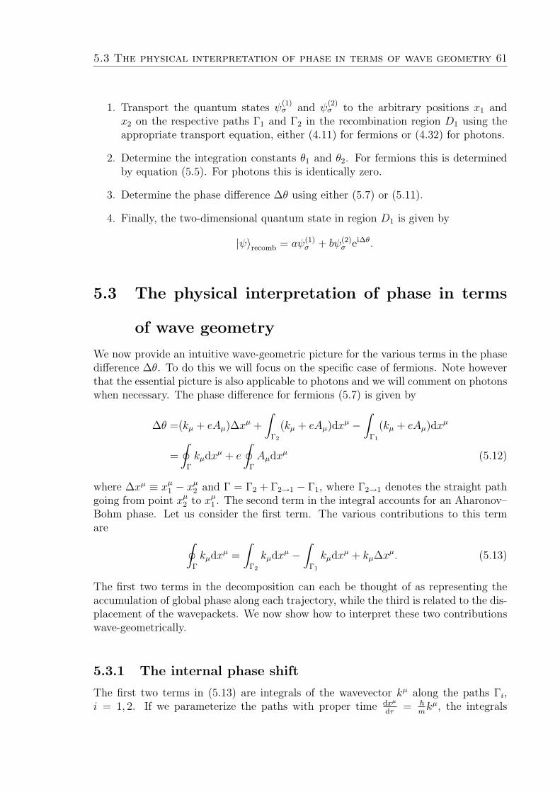
5.3 The physical interpretation of phase in terms of wave geometry 61

1. Transport the quantum states ψ(1)σ and ψ

(2)σ to the arbitrary positions x1 and

x2 on the respective paths Γ1 and Γ2 in the recombination region D1 using theappropriate transport equation, either (4.11) for fermions or (4.32) for photons.

2. Determine the integration constants θ1 and θ2. For fermions this is determinedby equation (5.5). For photons this is identically zero.

3. Determine the phase difference ∆θ using either (5.7) or (5.11).

4. Finally, the two-dimensional quantum state in region D1 is given by

|ψ〉recomb = aψ(1)σ + bψ(2)

σ ei∆θ.

5.3 The physical interpretation of phase in terms

of wave geometry

We now provide an intuitive wave-geometric picture for the various terms in the phasedifference ∆θ. To do this we will focus on the specific case of fermions. Note howeverthat the essential picture is also applicable to photons and we will comment on photonswhen necessary. The phase difference for fermions (5.7) is given by

∆θ =(kµ + eAµ)∆xµ +

∫Γ2

(kµ + eAµ)dxµ −∫

Γ1

(kµ + eAµ)dxµ

=

∮Γ

kµdxµ + e

∮Γ

Aµdxµ (5.12)

where ∆xµ ≡ xµ1 − xµ2 and Γ = Γ2 + Γ2→1 − Γ1, where Γ2→1 denotes the straight path

going from point xµ2 to xµ1 . The second term in the integral accounts for an Aharonov–Bohm phase. Let us consider the first term. The various contributions to this termare ∮

Γ

kµdxµ =

∫Γ2

kµdxµ −∫

Γ1

kµdxµ + kµ∆xµ. (5.13)

The first two terms in the decomposition can each be thought of as representing theaccumulation of global phase along each trajectory, while the third is related to the dis-placement of the wavepackets. We now show how to interpret these two contributionswave-geometrically.

5.3.1 The internal phase shift

The first two terms in (5.13) are integrals of the wavevector kµ along the paths Γi,i = 1, 2. If we parameterize the paths with proper time dxµ

dτ= ~

mkµ, the integrals


a) t1 b) t2

Figure 5.2: An illustration of the accumulation of internal phase from a time t1 (a) to alater time t2 (b) along a trajectory. The internal phase θint = ∆xint/o is determined by thedifference in the offset ∆xint = ∆x2 −∆x1 of a point pph of constant phase and a point penv

of constant position on the envelope at the two times t1 and t2. For timelike packet velocitiesthe phase velocity vph is greater than the group velocity vg = c2/vph < c so the internal phaseis seen to accumulate along the trajectory.

become ∫Γi

kµdxµ =

∫Γi

dτmc2

~. (5.14)

This results in a phase discussed in [28, 29] and motivated from the relativistic path in-tegral. We can also understand this term in a simple wave-geometric picture. Considera point penv(τ) defined by ϕ(x) = const which is fixed on the rigidly moving envelope(see figure 5.2). With respect to some arbitrary reference frame with 4-velocity nµ,the velocity at which penv moves in this frame is called the group velocity vg (see e.g.[63]), defined by u0 = e0

µuµ = γvg = (1 − v2

g/c2)−1/2, and corresponds to the particle’s

velocity. Secondly, consider a fixed phase point pph defined by θ(x) = const. The speedat which this phase point moves is given by vph ≡ c2/vg and is called the phase velocity.Thus, if vg < c the points of constant phase move with respect to the wavepacket. It isthis difference in velocity that results in the accumulation of the above mentioned pathintegral phase (5.14). To see this, first calculate how much distance δxint is gained bypph relative to penv during some time interval dt measured in this reference frame. Thisis given by

δxint = pph − penv =

(c2

vg

− vg

)dt.

In order to see how many radians of phase this distance is equivalent to we divide bythe reduced wavelength o ≡ ~/p = ~/mvg;

δxint

o=

(c2

vg− vg

)dt

o=

c2

vgγ−2dtmγvg

~=mc2

~γ−1dt =

mc2

~dτ.

During a finite period of time we have θint ≡∫

dτmc2/~ = ∆xint/o, which is nothingbut the path integral phase. We can now interpret the path integral phase as how muchthe constant phase surfaces have shifted inside the wavepacket. We call this an internalphase shift θint. When we add two wavepackets it is important to keep track of this

5.3 The physical interpretation of phase in terms of wave geometry 63

phase shift as it may lead to destructive or constructive interference. θint calculatedfor each trajectory is simply the integration constants θi(xi) (e.g. (5.5)).

Recall that for photons there was no contribution to the phase from the pathintegral, i.e. the integration constants are θi(xi) = 0. From a wave-geometric picturethis is due to the fact that the group and phase velocities are equal and thereforeθint = 0 .

5.3.2 The displacement induced phase difference

Let us now provide a wave-geometric interpretation for the third term in (5.13), kµ∆xµ.First, for simplicity let ∆xµ = xµ1 − x

µ2 be spacelike and orthogonal to some arbitrary

unit timelike vector nµ, i.e. ∆xµ = hµν∆xν where hµν = δµν − nµnν projects onto the

orthogonal space of nµ.3 kµ∆xµ then simplifies to:

|kµ∆xµ| = |kµhµν∆xν | = k⊥∆xdis| cos(α)| = ∆xdis

o

where k⊥ =√−hµνkµkν and ∆xdis =

√−hµν∆xµ∆xν , and we have used that | cos(α)| =

1 since the wavepackets are spatially displaced in the direction of motion, i.e. kµ⊥ ∝∆xµ.

Figure 5.3: Illustration of the recombination of two envelopes in the detector region D1.The offset of the classical positions x1, x2 of two wavepackets with the same wavelength oproduces a displacement phase of ∆θdis = ∆xdis/o.

This contribution to the phase difference, which is present for both fermions andphotons, can therefore be interpreted as the two wavepackets being spatially displaced,as illustrated in figure 5.3 and as argued in [35]. Note that in order for this displacementinduced phase difference ∆θdis = kµ∆xµ to be experimentally, the variance in ∆xdis overruns of an interference experiment must be significantly smaller than the wavelength o.Furthermore, if ∆xdis ∼ L (see Fig.5.1) then the interference effects will be drasticallyreduced and when ∆xdis ≥ L no interference phenomena will be present.

3∆xµ can always be made spacelike orthogonal by changing the arbitrary end points of the trajec-

tories Γ1 and Γ2.


5.3.3 Addition of quantum states in the wave-geometric pic-

ture

The recipe for adding two quantum states §5.2.3 can now readily be understood in termsof wave geometry. In the detector region D1 we have two wavepackets whose envelopes,centred at x1 and x2, overlap but are slightly offset (as in figure 5.3). Furthermore,each wavepacket has a rapidly oscillating phase that has evolved in a path-dependentway along each of the two distinct trajectories Γ1 and Γ2 (as in figure 5.2). Thesetwo effects produce respectively the displacement induced phase difference and theinternal phase difference. We then add these wavepackets to obtain the total phasedifference ∆θ. This is illustrated in figure 5.4. The total phase difference is again∆θTot = ∆θTrans. + ∆θ.

Figure 5.4: From a wave-geometric point of view we can understand the phase difference∆θ as the sum of two contributions: the difference in the internal phase given by ∆θint =∆xint/o and a phase difference ∆θdis = ∆xdis/o originating from the wavepackets beingspatially displaced.

5.4 Geometric phase

In the previous section we made a clear distinction between a phase shift induced bythe transport of a quantum state along a given curve from that which is obtained fromthe WKB approximation by considering the interference of two wave packets. In thissection we will like to expand on the transport induced phase shift. Consider (5.8) andfor clarity let us assume that the states |ψ(1)(Γ1)〉 and |ψ(2)(Γ2)〉 are the same stateup to phase, i.e. |〈ψ(1)(Γ1)|ψ(2)(Γ2)〉| = 1. Expanding (5.8) for electrons we get the

5.4 Geometric phase 65

following expression for ∆θTrans.

ei∆θTrans = uI σIA′AψA′ψC ×

T1 exp

[−∫

Γ1

dτ

(i

2uµωµIJ + iuIaJ − i

e

2mBrestIJ

)LIJ B

A

]×

T2 exp

[∫Γ2

dτ

(i


e

2mBrestIJ

)LIJ C

B

](5.15)

where T1,2 corresponds to the time ordering operator along Γ1,2, which is required sincethe infinitesimal transformations along the trajectory in general do not commute fromone instance to the next. In order to see that (5.15) must be true one can use that thetransport equation (4.13) preserves the inner product between states and as we shallsee is also unitary 6.1.1, hence the inner product between |ψ(1)(Γ1)〉 and |ψ(2)(Γ2)〉 isequivalent to the inner product between |ψ(1)〉 and |ψ(2)(Γ1 + Γ2)〉, where |ψ(2)〉 hasbeen transported backwards in time along Γ1.

Making use of the face that the two integrands by construction commute since byassumption |〈ψ(1)(Γ1)|ψ(2)(Γ2)〉| = 1 we get

ei∆θTrans = uI σIA′AψA′ψB T exp

[∮Γ

dτ

(i


e

2mBrestIJ

)LIJ B

A

](5.16)

Finally since the exponent is proportional to the identity we have

ei∆θTrans = Tr

[T exp

[∮Γ

dτ

(i


e

2mBrestIJ

)LIJ B

A

]](5.17)

We can now identify the various properties of what is generically known as geometricphase. The last term is closely related to the famous Berry phase [67]. This caneasily be seen by evaluating the term in the rest frame − i

2em

B · σ, hence provided thatthe magnetic field is changed adiabatically this would precisely correspond to a Berryphase. The first and second term are two additional geometric phases that arise for spinin the relativistic regime. The first is a purely geometric effect due to the spacetimecurvature where as the latter is due to the acceleration along the spacetime trajectory.Although the presence of the first phase has been suggested in the literature (althoughnot explicitly stated) the second phase is to our knowledge novel.

We can similarly obtain a geometric phase for the polarization qubit. By using thetransport equation for the Jones vector (4.45) we have

ei∆θTrans = Tr

[T exp

(∮Γ

dτuµWµAB

)]= Tr

[exp

(∮Γ

iuµWµdτσyAB

)](5.18)

Where the time ordered operator is no longer necessary since operators at differentpoints along a trajectory are always proportional to σy

AB and hence commute. Fur-

thermore for a closed trajectory where the initial and final states are the same we musthave either

∮Γ

iuµWµdτ = 2πn and hence ei∆θTrans = 1 or our initial state must be aneigenstate of σy

AB, i.e. the Jones vector corresponds to either left or right circular

polarization.


Figure 5.5: A Schematic diagram of a Neutron interferometer used in the COW experi-ment. A neutron incident on the first beam splitter BS1 is split into a spatial superpositiontravelling along two distinct paths Γ1 and Γ2. We find that Γ2 accumulates a phase shiftwith respect to Γ1 as it is higher in the gravitational field by ∆z.

5.5 An example: relativistic neutron interferome-

try

As a concrete example for implementing the above recipe for calculating the phasedifference we consider the gravitational neutron interferometry experiment illustratedin Fig.5.5, known as the Colella–Overhauser–Werner (COW) experiment [34]. Thesetup is geometrically identical to a Mach–Zehnder interferometer: The wavepacketis as usual split up into a spatial superposition and the respective wavepackets thentravel along two distinct paths. The interferometer is oriented such that one path ishigher up in the gravitational field relative to the other path. Essentially the two com-ponents of the spatial superposition have different speeds and experience two differentgravitational potentials, which leads, in the recombination region, to a phase shift.Interference fringes have been observed (see e.g. [32–34]) when the interferometer isrotated in the gravitational field, altering the difference in height of the paths.

In this section we are going to derive the phase difference for this experiment usingthe relativistic formalism developed above. The spin of the neutrons is ignored and wetreat them as scalar particles with no internal discrete degree of freedom. Thereforethere is no need to use the transport equation (4.11). The effects due to the spin couldbe included by computing (5.8); however the corrections to the overall phase differenceare minute, as noted in [36]. From this analysis we will arrive at an exact relativisticresult which contains, in certain limits, both approximate relativistic corrections to theCOW experiment [30, 31, 36] as well as the non-relativistic result [32–34].

One might represent the gravitational field for this experiment by the Schwarzschildmetric. However, since the size of the experimental apparatus is less than a metre andhence small compared to the curvature scale, we can mimic gravity by simply goingto an accelerated reference frame. This can be achieved by making use of the Rindler

5.5 An example: relativistic neutron interferometry 67

coordinates [61, 63] in which the flat spacetime metric takes the form4

gµν =

(1 + zg

c2)2 0 0 0

0 −1 0 00 0 −1 00 0 0 −1

.

Since the Rindler metric is static (i.e. independent of t) we have a Killing vectorηµ = (1, 0, 0, 0) and hence conserved energy E ≡ pµη

µ = mc2γg00, where γ ≡ (g00 −v2

c2)−1/2 with v the speed of the neutron as measured in the frame defined by the

Killing vector ηµ. We can now use this conserved energy to determine the speed v2

of the neutron in the upper path given the speed in the lower path v1, i.e. E1 =mc2γ1g00(z1) = mc2γ2g00(z2) = E2. We take the lower path to be at height z1 = 0, andso if the difference in height is ∆z we have the height of the top path being z2 = ∆z.Therefore we have the relation γ2g00(z2) = γ1 since g00(z1) = 1.

The easiest way to calculate the phase difference is by using the formula

∆θ =

∮Γ

kµdxµ =

∫Γ2

kµdxµ −∫

Γ1

kµdxµ + kµ∆xµ (5.19)

where we have used (5.7) and assumed that Aµ(x) is constant. This formula containstwo arbitrary spacetime points x1 and x2. Here we take these points to be where thetrajectories Γ1 and Γ2, respectively, hit the second beam splitter BS2. Since the spatialpositions of these two events are the same in our Rindler coordinate system we have∆xµ = (∆t, 0, 0, 0), where ∆t is the difference in arrival time. This is given by

∆t = `

(1

v1

− 1

v2

)where ` is the length of the horizontal legs of the paths. The contribution of the phasedifference from the third term is thus

kµ∆xµ =mc2`

~

(g00(∆z)γ2

v1

− g00(∆z)γ2

v2

)=mc2`

~

(γ1

v1

− γ1

v2

).

Let us now turn to the first and second terms in (5.19), representing the internal phaseshifts. Since the internal phases accumulated along the vertical components of eachpath are equal the quantity cancels in the calculation of the phase difference and soit is unnecessary to calculate them. The internal phase shifts of the upper and lowerhorizontal paths are given by

θ(1)int =

mc2

~τ1 =

mc2`

~1

γ1v1

, θ(2)int =

mc2

~τ2 =

mc2`

~1

γ2v2

.

4Note that we could also consider rotating reference frames which would lead to the Sagnac effect

[30, 33, 36], but for simplicity we will stick to the Rindler metric.


The phase difference is then given by

∆θ = θ(2)int − θ

(1)int + kµ∆xµ =

mc2`

~

(1

γ2v2

− 1

γ1v1

+γ1

v1

− γ1

v2

)which simplifies to

∆θ =m`γ1

~

(v1 −

v2

(1 + ∆zgc2

)2

)(5.20)

where we can make the replacement v2 = c√g00

(1− g00γ

−21

).

Eq.(5.20) is the exact result for the gravitationally induced phase shift in the Rindlermetric. This compares to various results in the literature [30–33, 36] for the gravita-tional effect in the COW experiment, which turn out to be approximations of (5.20).It is instructive to take various limits to demonstrate these connections.

Firstly, if we take the weak field limit, ∆zg/c2 1 we obtain

∆θ ≈ m`v1γ1

~

(1−

√1− 2

∆zg

v21

). (5.21)

If we furthermore take ∆zg/v21 1, which corresponds to assuming |v1 − v2|/v1 1,

and consider only first order terms, we obtain the phase result in [30]. If we insteadtake the non-relativistic limit (γ1 ≈ 1) we obtain the result of [31]. Expanding thisresult to two orders of ∆zg/v2

1 gives

∆θ ≈ m`

~

(∆zg

v1

+∆z2g2

4v31

), (5.22)

which indicates the ‘g2’ correction term derived in [31]. To leading order in ∆zg/v21 the

non-relativistic limit gives the standard theoretical prediction of the phase difference∆θCOW observed in the COW experiment

∆θCOW =m∆z`g

~v1

. (5.23)

There is a reported small discrepancy between measurement and theory [34]. However,the error introduced by neglecting corrections in ∆zg/v2

1 is too small to account forthis discrepancy [31].

The standard result (5.23) is obtained using a path integral approach (see e.g.[32, 33]). The path integral method allows only for summation over paths which startand end at the same two spacetime points. However, the classical trajectories in thisproblem in fact do not arrive at the second beam splitter at the same time. Therefore,the standard expression, although a very good approximation in the specific case ofthe actual experiment under consideration, is not exact even non-relativistically.

Let us examine a COW experiment numerically, presented in Table 5.1. From[32], the interferometer dimensions are ∆z = ` = 3.16 cm, the neutrons have mass

5.5 An example: relativistic neutron interferometry 69

Result Approximation Ref ∆ from COW ∆ from Exact

Exact Rindler (5.20) 1× 10−6 0

Weak field 1O ∆zg/c2 = 3× 10−18 (5.21) 1× 10−6 −1× 10−25

Small ∆v wf+1O ∆zg/v21 = 4× 10−8 [30] 2× 10−9 −1× 10−6

Non relativistic wf+0O γ = 1 + 2× 10−11 [31] 1× 10−6 −2× 10−9

g2 correction nr+2O ∆zg/v21 (5.22) 6× 10−7 −5× 10−7

[34] nr+1O ∆zg/v21 (5.23) 0 −1× 10−6

Table 5.1: Phase results for different approximations starting from the exact result (5.20)and finishing with the COW approximation (5.23). The Approximation column indicates towhat order a term is expanded (0O,1O,2O), the numerical value of the term, as well asindicating whether the phase result is based on previous approximations. For example, the‘Non relativistic’ result is zeroth order (‘0O’) in γ, but also possesses all of the Weak fieldresult’s approximations (‘wf’). The ∆ columns indicate the value of the result subtractingthe COW result, and the Exact result, respectively.

m = 1.67 × 10−27 kg and speed v1 = 2794 m.s−1, and g = 9.81 m.s−2. All results forphase difference ∆θ with these data give 55.6 rad. From 5.1, the difference betweenthe COW result (5.23) and the exact result (5.20) is 1.05 × 10−6 rad, a difference of19 parts per billion. The weak field limit is a very good approximation; 10−25 fromthe exact result. A nonrelativistic limit is the next best approximation (10−9 from theexact result), whereas the small velocity change first order expansion by [30] is lessjustified, providing only a relatively minor improvement on the COW result.


6Relativistically covariant quantum

information

6.1 Elementary operations and measurement for-

malism

In order to develop quantum information theory in curved spacetimes we need to under-stand how elementary operations such as unitary transformations and state updatingare represented within the reference frame covariant formalism of this paper. Thischapter is dedicated to these issues. In addition we show how Hermitian observablesare represented, how to calculate their expectation values, and in Chapter 7 we willshow how to construct explicitly a quantum observable for a Stern-Gerlach measure-ment.

6.1.1 Fermions

In this section we develop the notion of unitarity, observables and projectors forfermions. The notion of unitarity and observables is not straightforward for two rea-sons: (1) the inner product is velocity dependent and (2) Hilbert spaces associatedwith distinct points in spacetime must be thought of as separate. The formalism thatwe develop addresses these issues in a reference-frame-covariant way.

71

72 Relativistically covariant quantum information

Unitarity and Hermitian operators

Unitarity is traditionally defined for automorphisms U : H 7→ H, i.e. unitary mapstake elements from one Hilbert space back to the same Hilbert space. The map U isunitary if it satisfies

〈Uφ|Uψ〉 = 〈φ|ψ〉 (6.1)

where, for example the inner product for non-relativistic qubits is given by 〈φ|ψ〉 =δA′AφA′ψA. However, for our purposes this definition is too restrictive: we are interested

in localized qubits transported along some spacetime trajectory Γ. The Hilbert spacesassociated with the points along Γ must be thought of as distinct and the therefore amap induced by the transport equation (4.11) cannot be thought of as a map from aHilbert space to itself. Furthermore, the inner products for the Hilbert spaces dependon the respective 4-velocity. It is then clear that the transformation induced by thetransport equation (4.11) is not going to be unitary according to (6.1) as we are notdealing with automorphisms.

Consider therefore a map U : H1 → H2 where H1 and H2 are two Hilbert spaceson the trajectory Γ. A quantum state which belongs to H1 is indicated by a subscript|·〉1 and similarly for H2. The ‘generalized’ definition of unitarity then becomes

2 〈Uφ|Uψ〉2 = 1 〈φ|ψ〉1 (6.2)

using the inner product i 〈φ|ψ〉i = IA′A

uiφ

(i)A′ψ

(i)A , with IA

′Aui≡ u

(i)I σ

IA′A, and φ(i)A , ψ

(i)A ∈

Hi, i = 1, 2. If we adapt the tetrad such that uI = (1, 0, 0, 0) along the trajectory wesee that the inner product IA

′Au = uI σ

IA′A becomes the ordinary inner product δA′A

which is independent of both position and momentum. We would therefore expect theinner product between two quantum states along some trajectory Γ to be conserved.To see this let φ(τ) and ψ(τ) represent two quantum states that are Fermi–Walkertransported, according to equation (4.12) along Γ. Then we have

d

dτ〈φ|ψ〉 =

DFW

Dτ〈φ|ψ〉 = uI σ

IA′ADFW φA′

DτψA + uI σ

IA′AφA′DFWψADτ

= 0 (6.3)

since the Fermi–Walker derivative of uI is zero by construction, and the inner product〈·|·〉 is defined using IA

′Au(τ). Strictly speaking, the inner product should be labelled with

τ (i.e. τ 〈·|·〉τ ) in order to indicate that we are dealing with different Hilbert spaces.However, for convenience we omit this cumbersome notation.

Let us now consider a more general evolution dictated by a Schrodinger equation

DFWψADτ

=dψAdτ− i

(1

2

dxµ

dτωµIJ + uIaJ

)LIJ B

A ψB = iA BA ψB (6.4)

whereA BA represents some operator on ψB. Requiring the inner product to be preserved

under the evolution implies that A BA must for all φ, ψ ∈ H satisfy

uI σIA′AφA′A

BA ψB − uI σIA

′AA B′

A′ φB′ψA = 0 (6.5)

6.1 Elementary operations and measurement formalism 73

or equivalently 〈φ|Aψ〉 = 〈Aφ|ψ〉, which is nothing but the standard definition of aHermitian operator. Since this must hold for all φA and ψA we must have IB

′Au A B

A =IA′B

u A B′

A′ .In spinor notation we can define AA′A ≡ A A

B IA′Bu which yields an equivalent defi-

nition of Hermiticity for the spinorial object AA′A:

AA′A = AA′A.

An object AA′A satisfying this condition can be written as

AA′A = NI σIA′A (6.6)

for some real-valued coefficients NI . We also have A BA = IuAA′AA

′B where IuAA′ is theinverse of IA

′Au defined by IuAA′I

A′Bu = δBA . The corresponding operator A B

A is thengiven by

A BA ≡ IuAA′AA

′B = uIσIAB′NJ σ

JB′B = uINJ(σ[I σJ ] + σI σJ) BA= −2iuINJL

IJ BA + uIN

Iδ BA (6.7)

where LIJBA are the left-handed sl(2,C) generators and the term in δ B

A generateschanges in global phase 1. Using the self dual property Lαβ = 1

2iεαβγδLγδ [54, Eqn. 2.74]

to introduce the Pauli-Lubanski vector Wα(p) := 12εαβγδpβLγδ = ipβL

αβ, one can then

show that a Hermitian operator A must be of the form

A BA = NI

(−2W I B

A (p)

m+ uIδ BA

)(6.8)

where each operator is identified by a Lorentz 4-vector NI of real coefficients.2

It should be noted that the operator A BA does not ‘look’ Hermitian when written out

in matrix form. For example, A 21 6= A 1

2 . Rather, it is only the object AA′A ≡ IA′B

u A AB

which looks Hermitian in matrix form, i.e. AA′A = AAA′ 3. The reason for thisdifference can be clearly seen by expressing A B

A in the rest frame of the qubit. In theparticle rest frame, Hermitian operators are expressed as A B

A = NIσ0AA′σ

IA′B, and in

this case A 21 = ¯A 1

2 . Thus, from an operator ˆA which is Hermitian with respect to δA′A

we can construct another operator A which is Hermitian with respect to IA′A

u simplyby applying a boost, i.e. A B

A = Λ CA A D

C Λ−1BD , where Λ is the spin-1

2representation of

the Lorentz boost that takes δI0 to uI .A general inner product preserving evolution can therefore be understood as being

composed of two pieces. One piece, the Fermi–Walker derivative, dictates how accel-eration and the gravitational field affect the quantum state and has therefore a purely

1Note that one could also have chosen the right-handed representation RIJA′

B′ of the Lorentz group

as this would yield the same result.2This form will be used heavily in §73Spinor notation gives the relationship AA′A ≡ AAA′ ≡ AA′A between the conjugate and row-

column transpose.


geometric character. The Fermi–Walker derivative maps elements between neighbour-ing Hilbert spaces H(x,p)(τ) and H(x,p)(τ+δτ). The remaining term A B

A encodes possiblenon-geometric influences on the quantum state and is an automorphism A : H → H.This second term is required to be Hermitian with respect to the inner product IA

′Au .4

We have already seen an example of an evolution of the form (6.4). In the WKBlimit of the minimally coupled Dirac equation we arrived at the transport equation(4.11), where the Hermitian operator took on the form

B BA ≡ −

e

2mBIJL

IJ BA = − e

2mh KI h L

J FKLLIJ BA

where BIJ ≡ h KI h L

J FKL is the magnetic field experienced by the particle. To see thatthe magnetic precession term B B

A is Hermitian with respect to the inner product, weexpand the left side of the Hermiticity definition (6.5):

〈φ|Bψ〉 − 〈Bφ|ψ〉 = − e

2mφ(uK σ

KBIJ LIJ − BIJ

ˆLIJuK σK)ψ.

With BIJ real and making use of the identity [σK , LIJ ] = i[ηIJ σK − ηJK σI ] [39], wehave

〈φ|Bψ〉 − 〈Bφ|ψ〉 = − e

2muKBIJ φ[σK , LIJ ]ψ (6.9)

= −ie

2mφσKψ[uKB

II −B I

K uI ] = 0 (6.10)

since BIJuJ = 0 and B I

I = 0. The magnetic precession is thus a Hermitian automor-phism with respect to the inner product IA

′Au .

Observables and projective measurements

Observables are represented by Hermitian operators A BA , which will take the form

indicated in (6.8). The covariant expression of the expectation value of the observableA for a spinor ψA is given by

〈ψ|A|ψ〉 = ψA′NI σIA′AψA. (6.11)

where we have again used the identity IuAA′IA′Bu = δBA . Note that in (6.11) all indices

have been contracted, indicating the expectation value is manifestly a Lorentz invariantscalar and could in principle represent an empirically accessible quantity.

In order to complete the measurement formalism we need to discuss how to de-termine the post-measurement quantum state. We do this for the simple case ofprojection-valued measures, however we can easily extend the formalism to general-ized measurements. A Hermitian operator has a real eigenvalue spectrum and itsnormalized eigenstates |ψ(k)〉 are orthogonal, i.e.

〈ψ(k)|ψ(l)〉 = IA′A

u ψ(k)A′ ψ

(l)A = δkl.

4Hermiticity can alternatively be defined in terms of the partial d/dτ or covariant D/Dτ derivatives

but in doing so we would have to modify the definition of a Hermitian operator.

6.1 Elementary operations and measurement formalism 75

where k, l = ±. The spectral decomposition of an observable A is A BA =

∑± λ±P

±BA ,

where the λ± are the eigenvalues of A BA and the P±BA represents the corresponding

projector onto the eigenstate |ψ±〉. In spinor notation, the projectors are given byP±BA = IA

′Bu ψ±A′ψ

±A . A pair of projection operators P±BA which, together with the

identity operator, span the space of Hermitian observables on H can also be written as

P±BA =1

2(δ BA ∓ 2iuInJL

IJ BA ) (6.12)

with nInI = 1 and nIu

I = 0. These are the ordinary Bloch sphere projectors butwritten in a reference frame covariant way. One can then suspect that a measurementof spin along some unit direction can be represented by such projectors. This is indeedthe case as we shall see in Ch.7 for the specific case of a Stern-Gerlach measurements.Strictly speaking nIu

I need not be zero, this however only changes the global phase onthe updated state.

6.1.2 Photons

In this section we develop the notion of unitarity, observables and projectors for pho-tons. The definition of unitarity is much simpler than for fermions as the inner productis not velocity dependent; the difficulty is only in handling the gauge degrees of freedom,which as we shall see for the gauge invariant Jones vector is not relevant.

As we have already stated, the polarization state of a photon can be represented bya spatial complex 4-vector ψI orthogonal to the null wavevector kµ. Furthermore, thecorresponding quantum state of a photonic qubit with null velocity uI was identifiedas being a member of an equivalence class of polarization vectors ψI ∼ ψI + υuI allorthogonal to uI (§4.4.4). With the orthogonality condition and the gauge degree offreedom this space therefore reduced to a two-dimensional Hilbert space on which uni-tary and Hermitian operators act. We now develop the notion of unitarity, observablesand projectors within this four-dimensional formalism.

Unitarity and Hermitian operators

Unitarity and Hermiticity are more straightforward with polarization vectors thanspinors because the definition of unitarity 〈Uφ|Uψ〉 = 〈φ|ψ〉 is in terms of a stan-dard inner product ηIJ φ

IψJ where ηIJ is constant. The requirement for unitarityagain translates into requiring that the inner product between two polarization vectorsis conserved along trajectories, i.e.

d 〈φ|ψ〉dλ

=D 〈φ|ψ〉Dλ

=D 〈φ|Dλ

|ψ〉+ 〈φ| D |ψ〉Dλ

= 0. (6.13)

Consider now a Schrodinger evolution of the form

DψI

Dλ= βuI + iAIJψ

J orDψA

Dλ= iAABψ

B (6.14)


which is more general than the transport equation (4.32) or (4.45). Substituting into(6.13), we get

A JI φJψ

I − φIAIJψJ = 0 or A BA φBψ

A − φAAABψB = 0

where we have used that ψIuI = uIφI = 0. Requiring that this hold for all |φ〉 and |ψ〉we obtain the standard definition of Hermiticity; A I

J = AIJ or A AB = AAB.

For operators in the Jones vector representation we have no additional requirements.The Hermitian operator AAB is interpreted as acting on vectors in the subspace Sporthogonal to uµ. In the polarization vector representation we must, in addition to theabove, ensure that the gauge condition uIψ

I = 0 is preserved. This implies that

d(uIψI)

dλ=D(uIψ

I)

Dλ=DψI

DλuI = AIJψ

JuI = 0.

This condition ensures that Hermitian operators AIJ map polarization vectors intopolarization vectors. Again this should hold for all ψJ , so we have the conditionAIJuI ∝ uJ . The following two conditions suffice for characterizing a general Hermitianoperator;

A IJ = AIJ , (6.15a)

AIJuJ ∝ uI . (6.15b)

In order to determine the form of valid operators it is convenient to express thematrix AIJ in terms of the basis vectors uI , N I , eIA which spans the full tangentspace, where eIA = eIµe

µA is the diad expressed in the tetrad basis. A valid map AIJ

on polarization vectors must satisfy equations (6.15). In terms of the sixteen basiselements formed by the tensor product of each of the vectors, no terms in N I or NJ

can exist, since N IuI 6= 0. Any remaining terms that involve uI or uJ are pure gaugeand do not change the polarization vector. A hermitian operator is therefore, up togauge, represented as

AIJ = aAaBeIAe

BJ

where the two complex numbers aA constitute the four remaining real degrees offreedom. The two conditions in (6.15) thus reduce a 4 × 4 hermitian matrix to ef-fectively a 2 × 2 hermitian operator that acts on the transverse spacelike (polariza-tion) degrees of freedom. The relationship with the Jones vector is then given byAAB = aAaB = Caσ A

a B, where Ca consists of four coefficients a = 0, 1, 2, 3 and σacorresponds to the four Pauli matrices.

Observables and projective measurements

The construction of observables and projectors is identical to that of fermions. Observ-ables are represented by Hermitian operators AIJ or AAB. Let P I

(k)(PA(k)) represent the

6.2 Quantum entanglement 77

eigenvectors of AIJ(AAB). The∣∣P(k)

⟩form an orthonormal basis with

⟨P(k)|P(l)

⟩= δkl.

The probability pk of getting outcome λk is given by

pk = |P I(k)ψI |2 = |PA

(k)ψA|2. (6.16)

The corresponding projector for an eigenvector∣∣P(k)

⟩is P =

∣∣P(k)

⟩ ⟨P(k)

∣∣ and the

post-measurement state, up to gauge, is given by |ψ〉 → |ψ′〉 = P |ψ〉.In the case for photons in the polarization vector formalism we have a clean inter-

pretation of the eignevectors P Ik as polarizer vectors: complex, spacelike normalized

vectors5. Polarizer vectors correspond to the physical direction and parameters of anoptical polarizer: A linear polarizer direction is of the form eiθP I with P I real, anda circular polarizer is a complex vector P I = 1√

2(P I

1 + iP I2 ) with P I

1PJ2 ηIJ = 0 and

P I1P

J1 ηIJ = P I

2PJ2 ηIJ = −1. The probability of transmission of a polarization vector

through a polarizer is simply the modulus square of the overlap of the polarizationstate with the polarizer vector (6.16). Such an overlap clearly does not depend on thetetrad frame used, and indeed all indices are contracted in (6.16). The probability pis then manifestly a Lorentz scalar. It is easy to verify that the formalism is invariantunder gauge transformations ψI → ψI + υuI and P I → P I + κuI . Thus, the prob-ability p is both gauge invariant and Lorentz invariant as should be the case. Withthis completed measurement formalism we now have a complete framework for bothphotons and fermions to consider quantum information in the relativistic regime.

6.2 Quantum entanglement

Until now we have been concerned with the question of how the quantum state ofsome specific physical realization of a single qubit is altered by moving along somewell-defined path in spacetime. We shall now show how this formalism can easily beextended to describe entanglement of multiple qubits.

6.2.1 Bipartite states

We have seen that it is necessary to associate a separate Hilbert space with each pair ofposition and momentum (xµ, pµ). A single qubit moving along a specific path xµ(λ) inspacetime will therefore have its state encoded in a sequence of distinct Hilbert spacesassociated with the spacetime points along the path 6. The formalism that we have

5Note that P Ik need not be orthogonal to the photons velocity, P IψI = P Ih JI ψI = 0, hence it is

only the projected vector hIJPJk , or if you like PA which is physically significant.

6Recall that while we can uniquely determine the 4-momentum pµ = mdxµ

dτ from the trajectory

x(τ) in the case of massive fermions, the same is not true for photons. Due to the arbitrariness of

the parametrization of the null trajectory x(λ) we can only determine the null momentum up to a

proportionality factor, i.e. pµ ∝ dxµ

dλ .


so far developed determines how to assign a quantum state to each distinct Hilbertspace along the path along which we move the qubit. The one-parameter family ofquantum states |ψ(λ)〉 is parameterized by some parameter λ of the path x(λ), andthe sequence of Hilbert spaces associated with the path is H(x,p)(λ). The quantum state|ψ(λ)〉 belongs to the specific Hilbert space H(x,p)(λ).

Let us now consider how to generalize the formalism of this paper to the quantumstate of two, possibly entangled, qubits in curved spacetime. Instead of one worldlinewe will now have two worldlines, x1(λ1) and x2(λ2), and consequently instead of oneparameter λ we now have two, λ1 and λ2. Corresponding to each value of λ1 and λ2

we have two spacetime points and two Hilbert spaces, H(x1,p1)(λ1) and H(x2,p2)(λ2). Itis therefore clear that the quantum state describing the two qubits is mathematicallydescribed by a quantum state |ψ(λ1, λ2)〉 ∈ H(x1,p1)(λ1) ⊗ H(x2,p2)(λ2) which belongs tothe tensor product Hilbert space.

In order to calculate statistics (e.g. correlation functions) we need to provide aninner product for the tensor product Hilbert spaceH(x1,p1)(λ1)⊗H(x2,p2)(λ2). The naturalchoice is the inner product induced by the inner products for the individual Hilbertspaces.

In the case of fermions the natural choice for the parameterization λ is the propertime τ . The Hilbert spaces H(x1,p1)(τ1) and H(x2,p2)(τ2) have the inner products given byIA′A

1 = u1I σ

IA′A and IA′A

2 = u2I σ

IA′A where u1I and u2

I are the respective 4-velocities. Inour index notation a bipartite quantum state can be represented by an object with twospinor indices ψA1A2(x1(τ1), x2(τ2)). Note however that the indices A1 and A2 relateto two distinct spinor spaces associated with two distinct points x1(τ1) and x2(τ2) andtherefore cannot be contracted. The inner product between two bipartite quantumstates |ψ〉 and |φ〉 becomes

〈ψ|φ〉p1,p2= u1

I σIA′1A1u2

J σJB′2B2ψA′1B′2φA1B2 .

where p1, p2 are the momenta of the two qubits. In the case of photons the quan-tum state |ψ〉 can be represented by a polarization 4-vector ψI(λ) or Jones vectorψA(λ). A bipartite state |ψ〉 is then given by a two-index object ψI1I2(x1(λ1), x2(λ2))or ψA1A2(x1(λ1), x2(λ2)), where I1/A1 and I2/A2 belong to two different tangent spacesand thus cannot be contracted. The requirement that the polarization vector be or-thogonal to the null wavevector generalizes to uI1ψ

I1I2 = 0 = uI2ψI1I2 . The inner

product between two bipartite quantum states |ψ〉 and |φ〉 becomes

〈ψ|φ〉p1,p2= ηI1J1ηI2J2ψ

I1I2φJ1J2 = δA1B1δA2B2ψA1A2φB1B2 .

We could also consider bipartite states |φ〉 where one component is an electron and theother is a photon. Mathematically this would be represented as φI1A2

(x1(λ), x2(τ)) andlikewise for the Jones vector. The inner product can be constructed similarly.

Let us now turn to the evolution of bipartite quantum states. The physicallyavailable interactions of the qubits are given by local operations. Mathematically thismeans that the most general evolution of the state vector is given by two separate


Schrodinger equations:

iDT

Dλ1

|ψ(λ1, λ2)〉 = A1(λ1)⊗ I|ψ(λ1, λ2)〉 (6.17)

iDT

Dλ2

|ψ(λ1, λ2)〉 = I⊗ A2(λ2)|ψ(λ1, λ2)〉 (6.18)

where A1(λ1) and A2(λ2) are possible local Hermitian operators (as defined in §6.1)acting on the Hilbert spaces H(x1,p2)(λ1) and H(x2,p2)(λ2). D

T/Dλ denotes the transportlaw, i.e. the Fermi–Walker transport for fermions or the parallel transport for photons.

This mathematical description of the evolution of the quantum state is not standardsince we have two Schrodinger equations rather than one. However, if we introducean arbitrary foliation t(x) these two equations can be combined into one Schrodingerequation. First we express the parameters as functions of the foliation λ1 = λ1(t) andλ2 = λ2(t). This allows us to write the quantum state as only depending on one timeparameter: |ψ(t)〉 = |ψ(λ1(t), λ2(t))〉. The evolution of the quantum state now takes amore familiar form

iDT

Dt|ψ(t)〉 ≡ i

(dλ1

dt

DT

Dλ1

+dλ2

dt

DT

Dλ2

)|ψ(λ1(t), λ2(t))〉

=

(dλ1

dtA1 ⊗ I +

dλ2

dtI⊗ A2

)|ψ(λ1(t), λ2(t))〉

= A|ψ〉

where A ≡ dλ1

dtA1⊗ I + dλ2

dtI⊗ A2 is the total Hamiltonian acting on the full state. For

this single Schrodinger equation to hold for all paths xµ1(λ1) and xµ2(λ2), and all choicesof foliation t(x), and so for all values of dλ1

dtand dλ2

dt, it is necessary that both equations

(6.17) and (6.18) hold. Thus, the two mathematical descriptions of the evolution ofthe quantum state are equivalent when only local operations enter in the evolution.

If the Hamiltonian is not a local one, i.e. not of the form A = aA1 ⊗ I + bI ⊗ A2,then it is not possible to cast it into the previous form with two independent evolutionequations and it is also necessary to introduce a preferred foliation. However, if allinteractions are local the introduction of an arbitrary foliation is not necessary.

The generalization to multipartite states is straightforward. Furthermore, if weare dealing with identical particles the wavefunction should be symmetrized or anti-symmetrized with respect to the particle label, depending on whether we are dealingwith bosons or fermions. This will correctly reproduce for example the Pauli exclusionphenomenon and the Hong–Ou–Mandel bunching phenomenon [68].

6.2.2 State updating and the absence of simultaneity

Let us now discuss the issue of state updating for entangled states. Let Γ1 and Γ2 betwo spacetime trajectories along which two qubits are being transported. Furthermorelet x1(λ1) and x2(λ2) each represent a distinct point on the corresponding trajectory.


Consider now that the two qubits are in the entangled state

|ψ(λ1, λ2)〉 =1√2

(|+, λ1〉 |−, λ2〉 − |−, λ1〉 |+, λ2〉) .

If a measurement on qubit 1 is carried out at the spacetime point x1(λ1) with outcome‘+’, the bipartite state has to be updated as follows:

|ψ(λ1, λ2)〉 → |+, λ1〉 |−, λ2〉 .

Note that the value of λ2 is left completely arbitrary after the state update. It shouldtherefore be clear that even though the state update is associated with a distinctspacetime point x1(λ1) on the trajectory Γ1 no such point can be identified for Γ2. Inother words, as long as the local unitary evolution for particle 2 is well-defined, thestate updating can be thought of as occurring at any point x2(λ2) along Γ2. The pointx2(λ2) could be in the past, elsewhere, or in the future of x1(λ1). The reason for thisfreedom in state updating is that a projection operator on particle 1 commutes withany local unitary operator acting on particle 2.

6.2.3 An example: quantum teleportation

As an example of entanglement and state updating let us look at quantum teleportationin a curved spacetime. Although the mathematics is virtually the same as for the non-relativistic treatment, the interpretation is more delicate. In particular, in a curvedspacetime the claim that the input state is in some sense the “same” as the outputstate seems to lack a well-defined mathematical meaning. However, as we are goingto see, in order to carry out the standard teleportation protocol the parties involvedmust first establish a shared basis in which the entangled state takes on a definite andknown form. For example, Alice and Bob could choose the singlet state. This willbe called the ‘canonical’ form of the entangled state. Once this shared basis has beenestablished, Alice and Bob have a well-defined convention for comparing quantumstates associated with these different points in spacetime. The problems associatedwith quantum teleportation in curved spacetime are therefore similar to the problemsassociated with teleportation in flat spacetime when the maximally entangled state isunknown [69–72].

Consider then three qubits moving along three distinct trajectories Γ1, Γ2, and Γ3.For concreteness assume that the qubits are physically realized as the spins of massivefermions. The tripartite state is then given by

|Υ;λ1, λ2, λ3〉 ∈ H(x1,p1)(λ1) ⊗H(x2,p2)(λ2) ⊗H(x3,p3)(λ3)

or, written in our index notation, ΥA1A2A3(λ1, λ2, λ3).In order to proceed we define a basis for each one of the three Hilbert spaces

H(x1,p1)(λ1), H(x2,p2)(λ2), and H(x3,p3)(λ3) and for all points along the trajectories Γ1, Γ2,and Γ3. The three pairs of basis vectors are assumed to be orthonormal, and to evolveaccording to the local unitary evolution (e.g. by pure gravitational evolution given by


the Fermi–Walker transport (4.12)). Therefore, once we have fixed the basis for particlei at one point xi(λi) on the trajectory Γi, the basis is uniquely fixed everywhere elsealong the trajectory, at least where the local unitary evolution is well-defined. It followsthat a state can be expressed as a linear combination of these basis states with thecomponents independent of λi, i = 1, 2, 3.

We denote these three pairs of (one-parameter families of) orthonormal states as

φ(i)Ai

(λi) and ψ(i)Ai

(λi), with i = 1, 2, 3. The orthonormality conditions are explicitly givenby ⟨

φ(i);λi|ψ(i);λi⟩

= u(i)IiσIiA

′iAiφ

(i)

A′i(λi)ψ

(i)Ai

(λi) = 0⟨φ(i);λi|φ(i);λi

⟩= u

(i)IiσIiA

′iAiφ

(i)

A′i(λi)φ

(i)Ai

(λi) = 1⟨ψ(i);λi|ψ(i);λi

⟩= u

(i)IiσIiA

′iAiψ

(i)

A′i(λi)ψ

(i)Ai

(λi) = 1

with i = 1, 2, 3.

Consider now the specific tripartite three-parameter family of states

ΥA1A2A3(λ1, λ2, λ3) =1√2

(αφ

(1)A1

(λ1) + βψ(1)A1

(λ1))(

φ(2)A2

(λ2)φ(3)A3

(λ3) + ψ(2)A2

(λ2)ψ(3)A3

(λ3))

(6.19)where α and β are independent of λ1 (since evolution is entirely in the basis vectors)and |α|2 + |β|2 = 1. The maximally entangled state (involving particles 2 and 3) onlyhas coefficients equal to 0 or 1 which are trivially independent of the parameters λ2

and λ3. We will call the maximally entangled state in equation (6.19) the canonicalform. Other choices of this canonical form are possible but the teleportation protocolused below (see (6.20)) will then change accordingly.

As in the flat spacetime description we now proceed to rewrite the state in the Bellbasis for the Hilbert space H(x1,p1)(λ1) ⊗H(x2,p2)(λ2):

Φ±A1A2(λ1, λ2) ≡ 1√

2

(φ

(1)A1

(λ1)φ(2)A2

(λ2)± ψ(1)A1

(λ1)ψ(2)A2

(λ2))

Ψ±A1A2(λ1, λ2) ≡ 1√

2

(φ

(1)A1

(λ1)ψ(2)A2

(λ2)± ψ(1)A1

(λ1)φ(2)A2

(λ2)).

In these new bases the state |Υ〉 reads

ΥA1A2A3(λ1, λ2, λ3) =1

2

(Φ+A1A2

(αφA3 + βψA3) + Φ−A1A2(αφA3 − βψA3)

+ Ψ+A1A2

(βφA3 + αψA3) + Ψ−A1A2(−βφA3 + αψA3)

).

Alice now performs a Bell basis measurement on the particles 1 and 2. It is importantto note that the specific physical measurement operation that Alice needs to carry outdepends on the bases (φ

(1)A1, ψ

(1)A1

) and (φ(2)A2, ψ

(2)A2

). The basis (φ(2)A2, ψ

(2)A2

) is determined bythe maximally entangled state. If Alice does not know the maximally entangled stateshe will not be able to do the correct Bell basis measurement.


The outcome of the Bell basis measurement (Φ+, Φ−, Ψ+, or Ψ−) is then commu-nicated to Bob’s side: Bob performs the local unitary operation U (which is assumedto act on the state but not on the basis) given by

U =

1l if Φ+

σz if Φ−

σx if Ψ+

iσy if Ψ−

(6.20)

where σx, σy, σz take the usual form when expressed in the local orthonormal basis

(φ(3)A3, ψ

(3)A3

). Thus, as was the case for Alice, in order for Bob to know which specificphysical operation to carry out, the basis has to be specified. Since the basis is deter-mined by the maximally entangled state, Bob must know the entangled state in orderto carry out his operations. Note that if the basis in which Bob applies the operationis incorrect, the state that Bob obtains at the end differs depending on the outcome ofthe Bell measurement. In the case where Bob implements the operation in the correctbasis, Bob’s state is given by αφA3 + βψA3 .

We should now ask whether we can sensibly view this protocol as a ‘teleportation’of a quantum state from Alice to Bob in the sense that Bob received the same stateas Alice sent. This hinges on there being a meaningful way of comparing quantumstates associated with distinct spacetime points. However, as we have already stressed,if spacetime is curved, sameness of quantum states cannot be established uniquely byparallel transporting one qubit to the other as this would depend on the specific pathalong which we transport the qubit.

On the other hand, the maximally entangled state, by determining the bases forit to take the canonical form, defines a shared spinor basis for Alice and Bob. If wechange the basis, the maximally entangled state would of course change accordinglyand would no longer take on the canonical form. Given a shared basis we have awell-defined way of comparing quantum states and in particular a well-defined way toclaim that they are the same or not. Thus, when we have a maximally entangled state,there is a natural way of comparing quantum states associated with distinct spacetimepoints. It is in using this convention for comparing quantum states that we can claimthat Bob did indeed receive the same quantum state, and therefore we can say thatthe state was in this sense teleported.7

In the case of fermions it is also easy to see that the maximally entangled state willalso establish a shared reference frame, i.e. a shared tetrad. This comes about becausefrom the left-handed spinor ψA by means of which the quantum state is expressed wecan construct the null Bloch 4-vector bI = σIA

′AψA′ψA. A maximally entangled statecan therefore be loosely understood geometrically as a kind of ‘non-local connection’.

7We note that all examples of experimentally produced entangled qubit pairs are produced in

localized spatial regions and distributed to the parties. The components of the entangled state will

then undergo local unitary evolution along each trajectory.

7Relativistic Stern-Gerlach measurements

In this chapter we will be concerned with the relativistic measurement of spin, thedetails in this section are based on the work presented in [73]. In the literature therehave been several proposals dating back to the 1960’s for relativistic spin operators andthese have been studied in the context of quantum field theory for various reasons (seee.g. [74–78]). More recently, these operators have been used in relativistic quantuminformation theory to predict measurement statistics for relativistic spin measurements[42, 79–83]. The approach of this paper will not follow these proposals. Rather we willfollow a strictly operational approach, where we will expand on results developed in[73, 84]. Specifically, we will derive the relevant spin operator for a Stern-Gerlachmeasurement of a relativistic massive fermion. Importantly, our operational approachyields a Hermitian spin operator which is mathematically distinct from these previousproposals.

The outline of this paper is as follows: We will begin by very briefly reviewingHermitian operators with an eye towards spin observables. We will then derive therelativistic Stern-Gerlach spin observable by modelling a Stern-Gerlach measurement.Firstly, the specific mathematical form of the Stern-Gerlach operator is establishedusing the transformation properties of the electromagnetic field. Next, to confirmthat this is indeed the correct operator we provide a detailed analysis of the Stern-Gerlach measurement process. We do this by applying a WKB approximation tothe minimally coupled Dirac equation describing an interaction between a massivefermion and an electromagnetic field. Making use of the superposition principle weshow that the +1 and −1 spin eigenstates of the proposed spin operator are split intoseparate packets due to the inhomogeneity of the Stern-Gerlach magnetic field. Wethen compare this operator with two alternative proposals for a spin operator foundin[42, 79]. We conclude by discussing the consequences for quantum tomography. Notethat throughout this chapter we will assume that we are working in flat spacetime andas such all quantities are expressed with flat spacetime indices (α, β . . .). The extension

83

84 Relativistic Stern-Gerlach measurements

to curved spacetime can be made by assuming that the measurement process occurs ina region that is sufficiently small compared to the spacetime curvature.

7.1 Hermitian operators and spin observables

Recall that an Hermtian operator is given by

A = 2inαuβLαβ + nαuβη

αβI = nα

(−2Wα(p)

m+ uαI

)(7.1)

where each operator is defined by a Lorentz 4-vector nα of real coefficients. We arenow interested in spin observables formed from Hermitian operators (7.1). In order todo this we require that a spin observable evaluated in the particle’s rest frame reduceto the non-relativistic expression niσ

i where ni is the normalised spin measurementdirection. This implies that nα in (7.1) is orthogonal to uα, i.e. we have the condition

uαnα = 0. (7.2)

The magnitude of nα only rescales the eigenvalues of the observable and without loss ofgenerality we can normalise it so that it is spacelike with n2 = −1. A spin observabletherefore reduces to

A = 2inαuβLαβ + nαuβη

αβI = −2nαWα(p)

m(7.3)

The task of determining a spin observable has been reduced to determining nα. We willnow look at how we can do this for the particular case of a Stern-Gerlach measurement.

7.2 Intuitive derivation of the Stern-Gerlach ob-

servable

The task now is to determine the correct spin observable for a Stern-Gerlach mea-surement in which the Stern-Gerlach apparatus and particle carrying the spin havea relativistic relative velocity. Given the measurement formalism and formation ofLorentz invariant expectation values outlined in the previous section, the problem ofdetermining a ‘relativistic Stern-Gerlach spin operator’ is reduced to simply determin-ing how nα is related to the direction of the Stern-Gerlach apparatus. This analysiswill follow [73].

7.2 Intuitive derivation of the Stern-Gerlach observable 85

7.2.1 The non-relativistic Stern-Gerlach experiment

Before we consider the relativistic case it is helpful to first review a standard non-relativistic Stern-Gerlach spin measurement represented by the arbitrary non-relativisticHermitian observable niσ

i. In this case a particle is passed though an inhomogeneousmagnetic field. This causes the wavepacket to separate into two packets of orthogonalspin, after which a position measurement records the outcome. In the rest frame of theparticle, the fermion is exposed to a magnetic field BSG

i = |BSG|bSGi for a short period

of time, which is the magnetic field as measured specifically in the Stern-Gerlach restframe, denoted by SG. The direction bSG

i of the magnetic field defines the quantizationdirection of the spin, and the gradient of the magnetic field ∇i|BSG| determines the rateand direction along which the wavepacket splits into eigenstates of bSG

i σi [60]. Therefore

in the non-relativistic case the measurement direction ni is simply the direction of themagnetic field in the Stern-Gerlach rest frame, bSG

i .

7.2.2 The relativistic Stern-Gerlach experiment

We now turn to the relativistic scenario. In this case the qubit is now moving throughthe Stern-Gerlach apparatus with relativistic velocity. Viewed in the rest frame ofthe particle, denoted RF, the measurement process is indistinguishable from the non-relativistic one described in §7.2.1. However, in this frame the fermion will experiencea transformed magnetic field BRF

i = |BRF|bRFi . The measurement direction is now given

by ni = biRF, giving a spin observable of bRFi σ

i.1 This spin observable is written in thespecific frame of the particle rest frame, and due to the transformation properties of themagnetic field, the relationship between bRF

i and the orientation of the Stern-Gerlachapparatus is nontrivial. The goal is now to arrive at a covariant expression of thespin observable in terms of the Stern-Gerlach direction bSG

α and the 4-velocities of theStern-Gerlach apparatus and the particle.

In order to do this we assume that the electromagnetic field generated consists ofpurely a magnetic field in the rest frame of the Stern-Gerlach device,

Fαβ = −εαβγδvγBδSG

∗∗=

(0 00 Bij

)(7.4)

where vγ is the 4-velocity of the Stern-Gerlach device and BδSG is the magnetic field

4-vector of the Stern-Gerlach device. The double star ‘∗∗’ of the right hand sideindicates that it has been evaluated explicitly in the frame where vα

∗∗= (1, 0, 0, 0),

i.e. the Stern-Gerlach rest frame in which the Stern-Gerlach magnetic 4-vector is givenby Bδ

SG

∗∗= (0, Bi

SG).

We can now determine the 4-vector BαRF defined by Bα

RF

∗= (0, Bi

RF), where ‘∗’ indi-

cates evaluation in the particle rest frame, uα∗= (1, 0, 0, 0). The covariant expression

1Similarly it is the gradient of the rest frame magnetic field ∇i|BRF| which now determines the

rate and direction along which the wavepacket splits.


for BαRF is given by Bα

RF ≡ −12εαβγδuβFγδ, which when inserted into (7.4) yields

BαRF =

1

2εαβγδuβεγδκλv

κBλSG = Bα

SG(v · u)− vα(BSG · u) (7.5)

with εαβγδεγδκλ = −2(δακδβλ − δαλδβκ) [61, p.87], and the notation a · b ≡ aαb

α indicatinga 4-vector scalar product. Considering a spin measurement using this magnetic field,the four-vector nα in (6.11) is now the normalized direction of the rest frame magneticfield:

nα(m,u, v) ≡ bαRF =Bα

RF

|BRF|(7.6)

where |BRF| :=√−Bα

RFBβRFηαβ, and from (7.5) we have bRF · u = 0, in agreement with

(7.2). By Eqn.(7.3) the relativistic spin operator is therefore given by

S BA := −bRF

α

2Wα BA

m, (7.7)

and the expectation value of the corresponding measurement is calculated using (6.11).Expectation values (6.11) are invariant under simultaneous Lorentz transformation ofboth particle and apparatus, and thus with only the relative velocity between theapparatus and qubit and the spatial orientation of the Stern-Gerlach apparatus, wecan calculate the expectation values corresponding to a relativistic Stern-Gerlach spinmeasurement.

7.3 WKB analysis of a Stern-Gerlach measurement

In section 7.2 we argued that in the particle rest frame the measurement process isindistinguishable to a non-relativistic one [60, 85]. From this analysis we saw that it isthe direction of the magnetic field, as seen in the particle rest frame, that determineswhich spin measurement is being carried out. That derivation used standard argumentsbased on classical relativity and nonrelativistic quantum mechanics (see also [73, 84]).

In this section we provide a more fundamental analysis of the relativistic Stern-Gerlach measurement process, using the minimally coupled Dirac equation in the WKBlimit. Our starting point is again the Van der Waerden equation (4.4). The two com-ponent field is then expanded, without loss of generality, as a superposition in theeigenbasis of the spin operator (7.7). Using the linearity of the Van der Waerden equa-tion, we can analyse each component of the superposition separately, and identify theclassical trajectories of each component. We will use this to show that an inhomoge-neous magnetic field results in the splitting of a localised wave-packet with arbitraryspin into two components of orthogonal spin. This analysis singles out (7.7) as therelevant spin operator for a relativistic Stern-Gerlach spin measurement.

7.3 WKB analysis of a Stern-Gerlach measurement 87

7.3.1 The WKB equations

A qubit physically realized by the spin of a massive fermion is described by the Diracfield, therefore our starting point will be the Dirac equation minimally coupled to theelectromagnetic field

iγαDαΨ = iγα (∂α − ieAα) Ψ = mΨ (7.8)

where we define the U(1) covariant derivative as Dα ≡ ∂α− ieAα. Ψ is the Dirac field,γα are the Dirac γ-matrices and Aα is the electromagnetic four potential. Strictlyspeaking it is the positive frequency solutions of the Dirac equation that describe aone particle state. Furthermore we assume that the strength of the electric field isinsufficient to cause particle creation. We refer the reader to [73] for a discussion ofspin of a massive fermion as a realisation of a relativistic qubit.

We proceed with the WKB approximation by putting the Dirac equation (7.8) intoa second order form. In the Weyl representation of the Dirac matrices, the field splitsinto Ψ = (φA, χ

A′) [48]. The objects φA and χA′

are each two-component Weyl-spinorfields constituting left- and right- handed spinor representations of SL(2,C). In thisrepresentation the Dirac equation splits into two separate equations

iσαA′ADαφA = mχA

′(7.9a)

iσαAA′DαχA′ = mφA. (7.9b)

Solving for χA′

in equation (7.9a), inserting the result into (4.3b), and rearrangingyields a second order equation called the Van der Waerden equation [56]

ηαβDαDβφA − eFαβLαβ BA φB +m2φA = 0 (7.10)

where Fαβ = ∂αAβ − ∂βAα is the electromagnetic tensor and we have used that Lαβ =i2σ[ασβ] and ηαβ = σασβ.

The next step is to consider the Van der Waerden equation in the high frequencyWKB limit [73]. In this limit we see that the fermion travels along classical trajectories.We will assume that the field is sufficiently localised for the purposes of the Stern-Gerlach measurement.2 The goal then is to show that the wavepacket is split by theStern-Gerlach magnetic field into two packets of spin corresponding exactly to theeigenstates of the spin operator (7.7).

Traditional treatments of the WKB approximation begin with an ansatz for thespinor field of the form

φA(x) = ϕA(x)eiθ(x)/ε

where ε is to be thought of as a ‘dummy’ parameter whose only role is to identifythe different orders in an expansion. This ansatz is substituted into the Van derWaerden equation. One can then expand in the limit ε → 0; the high frequencylimit. Mathematically this corresponds to splitting the field into a rapidly varyingphase θ and a slowly varying envelope ϕA. The phase determines a field of wavevectors

2We refer the reader to [73] for further details on localisation.


kα ≡ ∂αθ − eAα which in this limit define integral curves along which the envelope istransported.

In the case of a Stern-Gerlach spin measurement we know the initial wave packetwill be split into two wavepackets of orthogonal spin with different wavevectors k±α ≡∂αθ

± − eAα. Therefore we must slightly modify the WKB ansatz to

φA = aϕ+Aeiθ+/ε + bϕ−Aeiθ−/ε (7.11)

where we have, without loss of generality, expanded the spinor field in the eigenbasisof S B

A (7.7) with components a, b ∈ C defined so that |a|2 + |b|2 = 1. The integralcurves are determined by the phases θ± which correspond to the spin eigenstates ϕ±A.We will see that these components are deflected in two different directions by theinhomogeneous magnetic field.

Using the linearity of the Van der Waerden equation we can analyze each componentφ±A = ϕ±Aeiθ±/ε separately. Substituting φ±A into (7.10) yields(

ηαβ∂α∂βϕ±A − eFαβL

αβ BA ϕ±B +

i

ε(2kα±∂αϕ

±A + ϕ±A∂αk

α±)

− 1

ε2k±α k

α±ϕ±A +m2ϕ±A

)eiθ±/ε = 0 (7.12)

where k±α ≡ ∂αθ± − eAα. It is customary to treat the mass term as ε−2 and we shall

do so here. In the ε→ 0 limit, which corresponds to large momentum, we notice thatthe electromagnetic field term Fαβ has a negligible influence in (7.12). Thus in orderfor the fermion to ‘feel’ the presence of the electromagnetic field, we will need to treatFαβ as a 1/ε term.

The WKB approximation proceeds by separating the orders of ε. For our purposeswe neglect the lowest order terms and thus obtain the following set of equations

1

ε

(2kα±∂αϕ

±A + ϕ±A∂αk

α± + ieFαβL

αβ BA ϕ±B

)= 0, (7.13)

1

ε2

(k±α k

α± −m2

)ϕ±A = 0. (7.14)

The first equation (7.13) will describe the evolution of the spin state of ϕ±A along atrajectory [73]. The second equation (7.14) determines the trajectories along whichthe fermion is transported. As it is, the spin does not couple to the magnetic field,implying that the trajectories cannot be spin-dependent, and thus no spin-dependentdeflection of packets can occur. However, if we treat the gradient of the magnetic fieldas a ε−2 term, we can include such a term in (7.14):(

k±α kα± −m2

)ϕ±A − εeFαβL

αβ BA ϕ±B = 0. (7.15)

To zeroth order in ε, Eqn.(7.15) is still the standard dispersion relation, and implies thatkα± is timelike. However, upon taking the gradient of (7.15), the second term becomesrelevant. It is in this way that the trajectories become spin-dependent, producing theseparation of the wavepacket that occurs in a Stern-Gerlach measurement.

7.3 WKB analysis of a Stern-Gerlach measurement 89

7.3.2 Determining the spin-dependent trajectories

It is from the integral curves ofdxα±dτ

= uα±(x) ≡ kα±(x)/m that we can read off thedeflection of the trajectories, where uα+ = uα− prior to entering the magnetic field. Inorder to deduce the implications of (7.15) we first multiply it by IA

′Au± ϕ±A′ , obtaining(

k±α kα± −m2

)|ϕ±|2 − εeFαβIA

′Au± Lαβ B

A ϕ±Bϕ±A′ = 0. (7.16)

Next, we decompose the operator FαβLαβ into the electric field ERF and magnetic field

BRF operators as measured in the rest frame defined by the initial 4-velocity u±α . Thisis given by

FαβLαβ = ERF + BRF

≡ 2u±γ uα±FαβL

γβ + Fαβh±αγh±

βδL

γδ(7.17)

where h±αγ ≡ δαγ − uα±u±γ is the spacetime projector onto the space orthogonal to the

4-velocity uα±. The first term is anti-Hermitian with respect to the inner product IA′A

u± ,whereas the second term is Hermitian.

First consider the magnetic field term BRF. Using the self-dual property Lαβ =12iεαβγδLγδ, and substituting the specific form (7.4) of the electromagnetic field of the

Stern-Gerlach apparatus, the expression can be rearranged to give

BRF =Fαβh±αγh±

βδL

γδ

=− 2iuαBRF

β Lαβ ≡ |BRF|S(7.18)

where |BRF| is the magnitude of the magnetic field as measured in the rest frame of u±α(7.5). We see that the magnetic field operator is in fact the relativistic spin operator(7.7) derived in the previous section multiplied by the field strength. Given that ϕ±Aare defined as eigenstates of this operator, (7.11), we therefore have that⟨

ψ±∣∣ BRF

∣∣ψ±⟩ = ±|BRF| (7.19)

where the quantum state is identified as |ψ±〉 ∼ ϕ±A/|ϕ±| with |ϕ±|2 ≡ ϕ±A′IA′Au± ϕ±A.

Let us now proceed to show that the expectation values of ERF in (7.17) with |ψ±〉are zero. Firstly, we define the projector Π±BRF

≡ 12(I ± 1

|BRF|2BRF), so we have⟨

ψ±∣∣ ERF

∣∣ψ±⟩ = Tr[ERF|ψ±〉〈ψ±|] = Tr[ERFΠ±BRF]

= Tr[ERF

1

2(I ± 1

|BRF|2BRF)].

Using the Lorentz invariance of the expectation values, we can evaluate the expectationvalues in the particle rest frame where the operators take on the form ERF ∗

= ERFi σi

and BRF ∗= BRFi σi: ⟨

ψ±∣∣ ERF

∣∣ψ±⟩ ∗= ± 1

|BRF|2ERF

i BiRF.


The electric field vector is given by EiRF

∗= F 0i = εijkvjB

SGk . By Eqn.(7.5), Bi

SG is alinear combination of Bi

RF and vi, and so we have EiRFB

RFi = 0. Therefore⟨

ψ±∣∣ ERF

∣∣ψ±⟩ = 0. (7.20)

Now substituting (7.19) and (7.20) into (7.16), and taking the gradient of the re-sulting equation, we obtain

0 = ∂α(k±β kβ±)± ∂α(|BRF|)

= 2kβ±∂βk±α + 2ekβ±Fβα ± ∂α(|BRF|) (7.21)

where we have used that ∂α(|BRF|) ∼ 1/ε2. We see thatdxα±dτ

= uα± = kα±/m must satisfy

md2xα±dτ 2

+ edxβ±dτ

F αβ ±

1

m∂α(|BRF|) = 0 (7.22)

whered2xα±dτ2 =

dxβ±dτ∂βu

α± is the 4-acceleration and uα±u

±α = 1. The first two terms of

(7.22) are simply the classical Lorentz force law, but in addition to this we have adeflection induced by the non-zero magnetic field gradient ±∂α(|BRF|)/m whose signdepends on whether the spin is parallel or anti-parallel to the magnetic field BRF

α .

The implications of (7.22) are as follows: prior to measurement we have that uα+ =uα−. The qubit is then exposed to a strongly inhomogeneous electromagnetic field Fαβfor a short period of time. This impulse-like interaction alters the velocity of therespective packets. For an ideal measurement this interaction is short enough thatnegligible precession of the spin, governed by (7.13), will occur during this splitting.The end result is the deflection of the ψ+

A component of spin with amplitude |a|2 in thedirection of the gradient of the magnetic field, and the deflection of the ψ−A componentwith amplitude |b|2 in the opposite direction. A position measurement will then producethe outcome ‘+’ with probability |a|2, and ‘−’ with |b|2. Thus we conclude that theoperator corresponding to relativistic Stern-Gerlach measurement is given by (7.7).

7.4 Comparison of spin operators

As we have already mentioned there have been various relativistic spin operators thathave appeared in the literature. These operators were originally developed in the con-text of quantum field theory for the purpose of splitting the spin degrees of freedomfrom the orbital angular momentum in a unique way which had important consequencesin developing a well defined position operator for a relativistic particle. It is only re-cently within the relativistic quantum information community where several authors[21, 25, 42, 79, 80, 82, 86] have considered the possibility that these operators couldcorrespond to an observable for ‘some’ spin measurement. In this section we will exam-ine two proposals for a relativistic spin operator first applied to Relativistic quantum

7.4 Comparison of spin operators 91

information by Terno [79] and Czachor[42], hence we will call them respectively theTerno and Czachor spin operator. The Terno operator is given by

S(B)

i :=1

m

[Wi −

W0pim+ p0

]. (7.23)

The Czachor operator is given by

S(C)

i :=Wi

p0

, (7.24)

Comparing these operators we will see that the operator derived in this section differsto both the Terno and Czachor spin operators.

The first distinction between the observables (7.23) and (7.24), and that for a Stern-Gerlach measurement (7.7) is that the former are defined in terms of 3-vectors (e.g.Wi, pi), i.e. they are defined in a specific reference frame, and in order to a comparethese we will need to either break the manifest Lorentz covariance of the Stern-Gerlachoperator or generalise the above to an arbitrary reference frame. We will here follow thelatter as this clearly highlights the similarities as well as the differences between theseoperators as well as highlight the features a measurement devices must have in orderto be mathematically represented by either (7.23) or (7.24). We would like to pointout that the analysis presented here in this thesis is the first time such a comparisonhas been made.

In order to generalise these operators we must first decide on the specific referenceframe with respect to which these operators are defined. There appears to be only twological choices either the rest frame of the measurement apparatus or the rest frameof the qubit. However we also require that a spin operator should correspond to aHermitian observable, i.e. we should have that (7.23) and (7.24) both reduce to thenon-relativistic spin operator σi in the rest frame of the qubit. We will therefore assumethat these two operators are defined in the rest frame of the measurement apparatusand identify the momentum pi as that corresponding to the momentum of the qubitas measured with respect to this frame.

As we have seen, an arbitrary Hermitian observables can always be expressed assome linear combination of the Pauli-Lubanski vector (7.1), i.e. aRF

α Wα BA . The goal

is therefore to identify the vector aRFα , which for the case of the Stern-Gerlach mea-

surement we found corresponded to to the direction of spin being measured as seenin the particles rest frame. We will therefore adopt this interpretation for aRF

α andhence denote it by ‘RF’. Recall that aRF

α must satisfy aRFα u

α = 0 and can geometricallybe thought of as the direction along the Bloch sphere one projects the spin. A rela-tivistic spin observable will simply define a relationship between aRF

α and the physicalquantities defining the measurement, such as the settings of a measurement apparatusaMAα (denoted ‘MA’) and the relative velocity between the measurement apparatus and

qubit. Note that in an arbitrary frame the relative veloocity will depend on the velocityof the measurement apparatus vα and the velocity/momentum of the qubit uα/pα.3

3Note that we will restrict our attention to cases where aMAα vα = 0, i.e. aMA

α is a spatial vector in

the measurement apparatus frame.


7.4.1 The Bogoliubov spin operator

The first operator we will consider was highlighted by [79] which follows the treat-ment by Bogoliubov in [87]. The spin operator is derived by defining three conditionsthat a relativistic spin-operator Si should satisfy: (1) it should reduce to the Paulimatrices in the non-relativistic limit; (2) it should be a 3-vector, so should transformunder rotations appropriately; and (3) it should satisfy the spin commutation rela-tions. These three conditions uniquely determine the Terno spin operator (7.23). Agiven measurement will correspond to an arbitrary linear combination of this operator

S (B) = −aRF

α

Wα(u)

m∗∗= aiS(B)

i . (7.25)

where we label the equality with ∗∗ for expression which have been evaluated in the

‘MA’ rest frame, i.e. where vα∗∗:= (1, 0, 0, 0). We therefore associate ai with the the

apparatus settings according to aαMA

∗∗= (0, ai). By making the right hand side of (7.25)

manifestly covariant we obtain the following relationship between aRFα and aMA

α

aαRF =

[aβMA −

uγaγMAv

β

uρ(uρ + vρ)

]hαβ (7.26)

where hαβ(u) = δαβ − uαuβ is the projector onto the space orthogonal to the 4-velocityuα. The spin observable is given by

S (B) = − 1

m

[aMA

α −uγaMA

γ vα

uρ(uρ + vρ)

]hαβW

β (7.27)

It is easy to see that in the MA frame (7.27) reduces to the right hand side of (7.25).The unique feature of this operator is that the settings of the measurement apparatusin fact corresponds to the same direction as seen by the qubit in the rest frame. Bythis means that for aαMA

∗∗= (0, ai) we have that aαRF

∗= (0, ai), i.e. the measurement

directions as seen in these two different frames are independent of the relative velocity.This should be contrasted with the Stern-Gerlach spin operator where the directionone aligns the Stern-Gerlach device biSG and the direction as seen in the rest-frame biRF

are momentum dependent and as a result do not in general coincide.

7.4.2 The Czachor spin operator

A second spin operator which we will compare has received considerable interest in therelativistic quantum information community. This operator was first applied to quan-tum information by Czachor [42] who studied the effect of Lorentz boosts on the degreeof violations of Bell inequalities on bipartite systems subjected to the measurementscorresponding to the spin operator (7.24).

S (C) = −aRF

α

Wα(u)

m∗∗= aiS(C)

i . (7.28)

7.4 Comparison of spin operators 93

Putting this in a manifestly Lorentz covariant form we have:

S (C) = −aRFα W

α

pαvα= −

aMAα hαβW

β

pαvα. (7.29)

We can now easily read off the relationship between aRFα and aMA

α for the Czachoroperator as

aαRF = hαβaβMA (7.30)

Unlike the Terno operator the motivation behind choosing S(C)

i as a relativistic spinoperator can be understood from physical grounds. Namely, by considering how aLorentz boost acts on the 3-vector ai. We have that

aiΛ(γβn)−→ a′

i= ai +

γ2β2

γ + 1(njaj)n

i

with ni the direction of the boost. If we then associate the direction ai as correspondingto the direction in which we align our measurement apparatus, the direction as seen inthe qubits rest frame is no longer ai but is in fact a′i. Therefore a suitable relativistic

spin observable which has an appropriate non-relativistic limit is defined as a′iσiγ

whereγ is the Lorentz factor. This can then be rearranged to give a linear combination ofthe Czachor spin operator S(C)

i .

7.4.3 Analysis of spin operators

Finally we would like to compare the two relativistic spin operators with the spinoperator corresponding to a relativistic Stern-Gerlach measurement derived in §7.2.Given that we have expressed the above operators in a manifestly Lorentz covariantway the comparison is rather simple. In terms of the Pauli-Lubanski vector we have

S BA = −bRF

α Wα BA

= −bSGα (v · u)− vα(bSG · u)√

(v · u)2 − (bSG · u)2Wα B

A . (7.31)

where we recall that bRFα = BRF

α / |BRF| and bSGα = BSG

α / |BSG|. We identify bRFα = aRF

α

and bSGα = aMA

α .There are several interesting features which we should point out. Firstly all op-

erators when expressed covariantly have the same standard form aRFα W

α BA . They are

hermitian operators which reduce appropriately to the non-relativistic spin operator.This should therefore not be used as a bench mark for whether a given operator iscorrect. The differences between these operators can be seen in how the directions aRF

α

and aMAα are related. For example in the case of a Stern-Gerlach measurement this

relationship was established by the transformation properties of the electromagneticfield. In regards to the operators (7.27) and (7.29) we clearly see that the relativisticobservable for a Stern-Gerlach measurement is mathematically distinct because the


0.0 0.2 0.4 0.6 0.8 1.0

0.6

0.4

0.2

0.0

0.2

0.4

0.6

Exp

ecta

tio

nV

alu

e

Spin Operator

Figure 7.1: Example of expectation value for spin operators as a function of relativevelocity β. Note that the Czachor and Stern-Gerlach expectation values are not alwayssymmetrically opposed.

relationship between aRFα and aMA

α is distinct. What must be addressed regarding theseoperators, if they are to be of any use, is how one might construct such a measurement,i.e. what physical setup would correspond to such measurements.

We would now like to highlight the empirical difference between the various spinoperators which will shed some light on the relationship between aRF

α and aMAα . Note

this analysis is similar to that found in [84] who compared S (SG) with yet another spinoperator. The first point to note is that the empirical difference between these operatorsis only noticeable for measurements which are not parallel or orthogonal to the directionof motion. In order to notice the greatest difference we choose our measurements to be45 to the direction of motion. Next one must choose an appropriate state. For statesorthogonal to both the direction of motion and the direction of measurement again nodifference is noticeable. In order to see the greatest difference we choose the rest framestate to be:

|ψ〉 = cos(π/8) |0〉+ sin(π/8) |1〉

When viewed in the non-relativistic limit on the Bloch sphere this would correspondto a measurement in an orthogonal direction to the state.

Calculating the expectation values as a function of the relative velocity betweenthe measurement apparatus and the qubits rest frame results in Figure 7.1. Note thatin order to make this comparison we have normalised the operators S (T) and S (C) suchthat the expectation values are in the range [−1, 1]

We see that the expectation values diverge between the various operators. Whatone finds, provided the appropriate state and measurement direction are chosen is thatthe expectation values between S (C) and S (SG) will diverge from each other. This isbecause the measurement direction aRF

α for S (C) projects onto the direction of motionwhere as the magnetic field bRF

α projects onto the space orthogonal to the direction ofmotion. While the expectation value for S (B) will always be independent of the relativevelocity vR because the corresponding direction aRF

α have been constructed so that itis independent of the vR. We therefore have shown that for an appropiate choice ofstates and measurements one can indeed distinguish between these operators.

7.5 Summary 95

7.5 Summary

In this chapter we provided two distinct ways of identifying the spin observable cor-responding to a Stern-Gerlach measurement of a massive fermion where the relativevelocity of the particle and Stern-Gerlach apparatus is relativistic. The first approachfollowed an intuitive argument based on the transformation properties of the electro-magnetic field. The second approach was a first-principles approach, starting with theDirac equation minimally coupled to the electromagnetic field. Using this equation weshowed that in the WKB limit the ‘+’ spin eigenstate of (7.7) is deflected ‘up’ and the‘−’ spin eigenstate is deflected ‘down’. We therefore concluded that in the relativisticregime the appropriate spin-operator for a Stern-Gerlach measurement is

S(v, p, bSG) = −bSGα (v · p)− vα(bSG · p)√

(v · p)2 − (bSG · p)2

2Wα(p)

m. (7.32)

Notably the spin operator (7.32) is momentum-dependent, so that, if the momentum isunknown, it is not possible to determine the expectation value. This has the followingimplications: Firstly, as we mentioned in §3.3 tracing over momentum of a state writtenin a tensor product basis of spin and momentum has been used in relativistic quantuminformation theory to extract the reduced spin density matrix [25–27, 82, 88, 89].However, we can see that due to the momentum dependence of the observable (7.32),this reduced spin density matrix is not useful for predicting the statistics of a relativisticStern-Gerlach measurement. The usefulness of the reduced spin density matrix isfurther limited by the fact that it has no Lorentz covariant transformation properties[21, 25, 26, 89–91].

Secondly, in attempting to perform quantum tomography of the spin degrees offreedom one faces an obstacle. The goal of quantum state tomography is to inferthe quantum state from the outcomes from a set of different measurements. Non-relativistically, the relationship between the quantum state and measurement data ismomentum independent, and it is enough to choose three linearly independent direc-tions in order to reconstruct the quantum state. However, in the relativistic Stern-Gerlach case, the experimental data are related to momentum dependent theoreticalexpectation values of the quantum state, determined by (7.32). Thus, if momentum isunknown, three linearly independent directions will not suffice. We leave it as an openquestion as to what minimal set of measurements is required to reconstruct the statein this relativistic case.

As a final point we discussed several alternative operators that are used as ob-servables for relativistic spin measurements. Two notable operators that have beenproposed in the relativistic quantum information community are the Terno (7.27) andCzachor (7.29) spin operators. Although we showed that indeed these proposals areHermitian they are mathematically distinct from (7.32) and it was shown that theylead to quantitatively distinct predictions. The question that therefore must be ad-dressed is whether there exists a non-trivial physical implementation for either of theseproposals. However, it is clear that measurements making use of the coupling of spinto the electromagnetic field will not yield these spin operators.


8Conclusion

This section of the thesis explored relativistic quantum information restricted to theregime of localized qubits where the particle number ambiguity is circumvented. A lo-calized qubit is therefore understood in this paper to be any object that can effectivelybe described by a position and momentum (x, p) and some two-component quantumstate |ψ〉. In particular, we obtained a description of localized qubits in curved space-times, with the qubits physically realized as the spin of a massive fermion, and thepolarization of a photon.

The original motivation for this research was to develop a formalism for answering asimple experimental question: if we move a spatially localized qubit, initially in a state|ψ1〉 at spacetime point x1, along some classical spacetime path Γ to another point x2,what will the final quantum state |ψ2〉 be? Rather than working directly with Wignerrepresentations, which as we have already stressed cannot be extended to curved space-time, our starting point in answering this question was the one-particle excitations ofthe quantum fields that describe these physical systems. The one-particle excitationsin curved spacetime satisfy respectively the Dirac equation minimally coupled to theelectromagnetic field, and Maxwell’s equations in vacuum. From these fields we wereable to isolate a two-component quantum state and a corresponding Hilbert space.

In the case of fermions §4.3, the equation governing the transport of the spin of afermion consisted of a spin-1

2version of the Fermi–Walker derivative and a magnetic

precession term, expressed in a non-orthonormal Hilbert space basis. This result wasexpected since an electron can be regarded as a spin-1

2gyroscope, and the precession

of a classical gyroscope along accelerated trajectories obeys the Fermi–Walker equa-tion. By introducing an orthonormal Hilbert space basis, which physically correspondsto representing the spinor in the particle’s rest frame, we reproduced the transportequation obtained in [17, 18] which made use of Wigner representations.

For photons §4.4, we showed by applying the WKB approximation to vacuumMaxwell equations that the polarization vector of a photon is parallel transported along

97

98 Conclusion

geodesics and that this corresponds to a Wigner rotation. Furthermore, this rotationis proportional to the spin-1 connection term ωµ12 when we consider a reference framewhere the photon 3-velocity is along the z-axis. In this way the effect of spacetimegeometry on the quantum state was easily identified. In addition and in contrast to thecase for fermions, we were able to constructed a representation which we referred asthe Jones vector ψA that is a unitary, gauge invariant and Lorentz covariant formalism.

In the case for fermions we worked with faithful finite-dimensional but non-unitaryrepresentations of the Lorentz group, specifically a two-component left-handed spinorψA. Nevertheless, by identifying a suitable inner product we obtained a unitary formal-ism by no-longer insisting on the need for a representation. The advantage of workingwith non-unitary representations is that the objects which encode the quantum statetransform covariantly under actions of the Lorentz group. As a result the transportequations are manifestly Lorentz covariant, in addition to taking on a simple form.The connection to the Wigner formalism for fermions was obtained by choosing a ref-erence frame adapted to the particle’s 4-velocity, which is the reason why the Wignerformalism is not manifestly Lorentz covariant.

For photons the situation was a little different, for fermions unitarity was restoredby introducing a Lorentz invariant inner product. For the Jones vector formalism thedifficulty is not with unitarity or Lorentz covariance, rather the difficulty is in insistingon a gauge invariant formalism. In particular, we showed that in order for the innerproduct to be gauge invariant we were required to only take the inner product betweenstates with the same momentum and as such our Hilbert space was again labelledby momentum Hp, and in the same way as for fermions the formalism is thereforeno longer a representation Lorentz group. With this insight we showed the transportequation in fact corresponds to a Wigner rotation, but not to that obtained in theWigner formalism, since the Jones vector is manifestly Lorentz convariant where asthe Wigner formalism is not.

A second advantage of working in terms of the Dirac and Maxwell fields instead ofthe Wigner representations is that global phases and quantum interference come outautomatically from the WKB approximation. By considering spacetime Mach–Zehnderinterference experiment we arrived at a general relativistic formula for calculating thegravitationally induced phase difference. In the specific case of gravitational neutroninterferometry we obtained a new general relativistic phase which reduced in variouslimits to existing relativistic and non-relativistc approximations for the gravitationallyinduced phase difference. Our overall approach, however, provides a general, unified,and straightforward way of calculating phases and interference for any situation. Inaddition we derived a new gravitationally induced geometric phase for fermions andusing the Jones vector formalism showed that no such phase exists for photons.

Using these two representations we then constructed in Chapter 6 a fully relativisti-cally covariant quantum information formalism. In particular we showed how to treathermitian operators, measurements and state updating, as well as the treatment ofmultipartite states, entanglement, and teleportation, thereby extending the formalismto include all the basic elements of quantum information theory.

One area that (with the exception of a few) has been neglected within the litera-ture was in regard to making empirical predictions, that is, we need a way to extract

99

probabilities for outcomes from the formalism. Such a measurement formalism wasdeveloped for both fermions and photons. The predicted probabilities of outcomes ofexperiments were shown to be manifestly Lorentz invariant and thus reference frameinvariant, resulting in a relativistically invariant measurement formalism. In addition,we identified the spin observable corresponding to a Stern-Gerlach measurement of amassive fermion where the relative velocity of the particle and Stern-Gerlach appara-tus is relativistic. This was shown in two distinct ways, the first approach followed anintuitive argument based on the transformation properties of the electromagnetic field.The second approach was a first-principles approach, starting with the Dirac equationminimally coupled to the electromagnetic field. Using this equation we showed thatin the WKB limit the ‘+’ spin eigenstate of (7.7) is deflected ‘up’ and the ‘−’ spineigenstate is deflected ‘down’. We therefore concluded that in the relativistic regimethe appropriate spin-operator for a Stern-Gerlach measurement is

S(v, p, bSG) = −bSGα (v · p)− vα(bSG · p)√

(v · p)2 − (bSG · p)2

2Wα(p)

m. (8.1)

Notably the spin operator (8.1) is momentum-dependent, so that, if the momentum isunknown, it is not possible to determine the expectation value. This has the followingimplications: Firstly, the effect of tracing over momentum of a state when written ina tensor product basis of spin and momentum, that is in the Wigner representationhas been has been a big area of interest in relativistic quantum information theory.In particular the fact that the reduced spin density matrix has no Lorentz covarianttransformation properties has been the source of many debates [21, 25–27, 82, 88–91].However, we can see that due to the momentum dependence of the observable (8.1),this reduced spin density matrix is not useful for predicting the statistics of a relativisticStern-Gerlach measurement.

Secondly, in attempting to perform quantum tomography of the spin degrees offreedom one faces an obstacle. The goal of quantum state tomography is to inferthe quantum state from the outcomes from a set of different measurements. Non-relativistically, the relationship between the quantum state and measurement data ismomentum independent, and it is enough to choose three linearly independent direc-tions in order to reconstruct the quantum state. However, in the relativistic Stern-Gerlach case, the experimental data are related to momentum dependent expectationvalues of the quantum state, determined by (8.1). Thus, if momentum is unknown,three linearly independent directions will not suffice. It would be very interesting to seeif it is possible to reconstruct a state given a set of measurement data, and if so whatis the minimal set of measurements required to reconstruct the state in this relativisticcase.

As a final point we discussed several alternative operators that are used as ob-servables for relativistic spin measurements. Two notable operators that have beenproposed in the relativistic quantum information community are the Terno (7.27) andCzachor (7.29) spin operators. Although we showed that indeed these proposals areHermitian they are mathematically distinct from (8.1) and it was shown that they leadto quantitatively distinct predictions. The reason behind this was due to the simple

100 Conclusion

fact that the measurement direction as seen in the rest-frame aRFα had different trans-

formation properties to that for a magnetic field and as a result these proposals cannotbe considered to represent a Stern-Gerlach measurement. The question that thereforemust be addressed is whether there exists a non-trivial physical implementation foreither of these proposals. However, it is clear that measurements making use of thecoupling of spin to the electromagnetic field will not yield these spin operators.

On reflection of this part of the thesis, we see that the the Lorentz group playeda primary role in the construction of qubits in curved spacetime. This role can beunderstood in terms of how gravity acts on physical objects. When an object is movedalong some path xµ(λ) in spacetime it passes through a sequence of tangent spaces.These are connected by infinitesimal Lorentz transformations that are determined fromthe trajectory and the gravitational field (i.e. the connection 1-form ω I

µ J). That is,apart from a possible global phase, this sequence of infinitesimal Lorentz transforma-tions determines how an object is affected by the gravitational field. In particular, ifthe object has internal degrees of freedom that transform under the Lorentz group, wecan determine the effect of gravity on the state of these internal degrees of freedom.For example, this is the explanation for the presence of spin connection terms in thefermion Fermi–Walker transport. It is also an explanation for why the photon Wignerrotation is simply a rotation of the linear polarization and so respects the helicity ofthe photon: no Lorentz boost can change frames sufficiently to change the helicity ofa photon.

In this paper we focused on just two physical realizations which constituted non-trivial representations of the Lorentz group. We can nevertheless contemplate otherrealizations such as composite two-level systems. In order to understand how gravityacts on the qubit state the same general approach applies: One needs to provide amathematical model of the physical system. Once a model is established one canin principle determine how (if at all) the quantum state transforms under a Lorentztransformation. In addition to this there are other possible gravitational influences onthe quantum state such as gravitationally induced phases.

As a concrete example of a physical realization that would behave very differentlyto the elementary realizations treated in this paper, consider a two-level system wherethe two levels are energy eigenstates |E1〉 and |E2〉. From ordinary non-relativisticquantum mechanics we know that the total state |ψ〉 = a |E1〉+ b |E2〉 will undergo theevolution

|ψ(t)〉 = aeiE1t/~ |E1〉+ beiE2t/~ |E2〉 .

If the composite object is much smaller than the curvature scale and the accelera-tion is sufficiently gentle to not destroy it we can obtain a fully general relativisticgeneralization by simply replacing the Newtonian time t with the proper time τ :

|ψ(τ)〉 = aeiE1τ/~ |E1〉+ beiE2τ/~ |E2〉 .

Thus, because of the energy difference we develop a relative phase between the twoenergy levels which is proportional to the proper time of the trajectory. In principlewe can make use of such a two-level system to measure the proper time of a spacetime

101

trajectory. Since proper time is path dependent we see that the transport of thequantum state is also path dependent, and we can also contemplate possible interferenceexperiments.

The formalism presented in this paper provides a basis for quantum informationtheory of localized qubits in curved spacetime. One theoretical application of this is toextend the applicability of clock synchronization [92–94] and reference frame sharing[70, 71] to curved spacetime, and provide an interesting physical scenario for the studyof symmetries in quantum mechanics [95, 96].

This formalism also has potential measurement applications. For example, in thelast ten or fifteen years there has been interest in precision measurement of the effectsof general relativity. Most recently there has been the experimental confirmation of thepredicted frame-dragging effect by Gravity Probe B [97].1 On the other hand, in thesame period there has been an increased interest in quantum precision measurementsusing techniques from quantum information theory [99–104]. The formalism of thispaper provides a bridge between these developments, providing a solid foundation forconsidering the effects of gravity on quantum states, and for considering the design ofprecision measurements of these effects. Importantly, by the use of entangled statesone can in principle significantly increase the precision of such a measurement. Forlocalized qubits in curved spacetimes as defined in this paper, the effect of gravity entersas classical parameters in the unitary evolution of the quantum state. Therefore, oneshould be able to use these same quantum information theory techniques to increasethe precision in measurements of the gravitational field. It is plausible that such anamalgamation of the transformation of the discrete degrees of freedom of a quantumstate and the phase accumulation, by increasing the degrees of freedom to be measured,will increase the sensitivity with which possible future sophisticated precision quantummeasurements can measure gravitational effects.

For example, spacetime torsion is generally believed, even if non-zero, to be toosmall to measure with present day empirical methods [59]. One problem is that tor-sion, as it is conventionally introduced in Einstein–Cartan theory, does not have anypropagating degrees of freedom. Thus, the torsion in a spacetime region is non-zeroif and only if the spin density is non-zero there. Experiments to measure torsion thusrequire objects to pass though a material with non-zero spin density to accumulate aneffect, while accounting for standard interactions. Needless to say, measuring torsion isthen very difficult. However, electrons decouple from matter in the high energy WKBlimit and effectively only feel the gravitational field including torsion. Thus, the spinof high energy fermions might carry information about the spacetime torsion.

To summarize: in this paper we have provided a complete account of the transportand measurement of localized qubits, realized as elementary fermions or photons, incurved spacetime. The manifest Lorentz covariance of the formalism allows for a rela-tivistic treatment of qubits, with a perhaps more straightforward interpretation thanapproaches based on Wigner representations. The treatment of multipartite states,entanglement and interferometry provides a basis for quantum information theory oflocalized qubits in curved spacetime.

1See also [20, 98] for a recent theoretical analysis of polarization rotation due to gravity.

102 Conclusion

Part II

103

9“Not all together desperate” - the Newton

Scholium Problem

The concept of time and duration has been of great interest in natural philosophydating back to Aristotle and remains so today [105–108]. For physicists however, suchnotions are typically believed to be well understood at least within the context of aphysical theory. That was, until the beginning of the research field formally referredto as canonical quantum gravity (the Hamiltonian quantization of general relativity)in 1968 [2]. This approach to quantum gravity, as well as many alternative approachessince, have, all been plagued by the infamous ‘problem of time’, and this has ledmany to think seriously about what is time and how it is treated in our physicaltheories [109–112]. In particular what is it about time in general relativity that isso different from other theories that makes it such a difficult theory to quantize? Toeven begin answering this question we need to understand precisely the relationshipbetween what we mean mathematically by ‘time’ in our physical theories and how thisis tied to the the measurements of duration. In this paper we will contribute to such aninvestigation by analysing the notion of time within the context of Newtonian physics,where surprisingly even within this ‘simple’ theory the notion of time, duration andclocks is still very mirky. In particular we will see that in order to arrive at a satisfactoryunderstanding of time and duration we will have to solve what Julian Barbour hasdubbed the Newton Scholium problem (see, e.g., [113], p. 1266).

The Scholium refers to a section in Newton’s Mathematical Principles of NaturalPhilosophy [114] and builds upon the careful definitions of terms that Newton presentsin the opening section of the Principia. In particular, he offers the following distinction

I. Absolute, true, and mathematical time, of itself, and from its own nature,flows equably without relation to anything external, and by another nameis called duration: relative, apparent, and common time, is some sensible

105

106 “Not all together desperate” - the Newton Scholium Problem

and external (whether accurate or unequable) measure of duration by themeans of motion, which is commonly used instead of true time; such as anhour, a day, a month, a year. ([114], p.6)

Newton introduces two distinct notions of time, namely absolute and relative time.Absolute time is purely mathematical in character and by definition is a unique mea-sure, at least up to a choice of units. On the other hand relative time is tied to themeasurements and observations of the physical world around us. As such, there is nounique choice, any measure will suffice as a notion of relative time, e.g. one could usea swinging pendulum or equally as valid the motion of the moon. We will refer to adevice that reads relative time as a clock and a clock whose readings coincide withabsolute time as an accurate clock.

Given that these two times are in general distinct and should not be assumed to beequivalent, we have to ask an important but yet very elementary question: does thesymbol t in Newton’s equations of motion

mkd2xkdt2

= Fk (9.1)

refer to absolute or relative time? Put differently, does the symbol t correspond directlyto the readings of some external physical clock or does it represent Newton’s moreabstract absolute time?

From a logical point of view we are free to adopt any of the two interpretations ofthe symbol t, but a moment’s reflection reveals that when carrying out elementary me-chanical experiments, it is almost universally assumed that the symbol t represents thereading of a laboratory clock, i.e. an external device which is not modelled explicitlyby the equations of motion describing our physical system in question. This interpre-tation of the symbol t corresponds to what Newton calls relative time (or commontime). Notably, this operational interpretation of t is also the one adopted by Einsteinin his seminal paper on special relativity in which clocks (and rods) are treated asself-sufficient primitive objects [108, 115].1

Let us illustrate these remarks by an example. Consider a swinging pendulum, theequation of motion describing our physical system is

d2θ

dt2= −g

rcos θ. (9.2)

In this example the symbol t could represent relative time, i.e. the readings of anexternal laboratory clock. However we here face an immediate issue, as we have alreadypointed out there is no unique choice of a suitable clock. The only privileged choicewould be if the clock is accurate.

Even if we assume the clock is accurate any real physical clock consists of manyinternal degrees of freedom. In this example however, the external clock is mathemati-cally represented only by one real number t. In particular, the equation (9.2) does not

1Although Einstein did later criticize the idea of taking clocks and rods as self-sufficient entities

[116].

9.1 Theory of clocks and their accuracy 107

contain any dynamical degrees of freedom of the external clock. Obviously, the clockwith all its internal degrees of freedom, is not faithfully modelled within the theory.Therefore, the assumption that the clock is accurate (i.e. that the rate of ticking re-mains uniform over time and is hence in sync with absolute time) cannot be justifiedwithin our pendulum theory. Rather, the accuracy of the clock has to be taken ontrust; perhaps we trust the clock manufacturer. The question we would like to addresshere is how do we measure duration and how do we determine its accuracy? We willsee that addressing this fundamental question will ultimately lead to the Scholiumproblem. Simply stated the Newton Scholium problem is as follows: do the Newtonianequations of motion allow us, given a set of observations, to deduce the presence ofabsolute time or space?

In this paper we aim to give a modernized presentation of the Newton Scholiumproblem. In particular, we will formalise this traditionally philosophical problem math-ematically, with a view to exposing its foundations and stating exactly what it wouldtake to resolve this long lasting problem that remains to this day. We also draw onhistorical and philosophical lessons from our analysis highlighting, in particular, theextent to which the sophistication of Newton’s understanding of time and its measure-ment has been radically underestimated.

The outline of this chapter is as follows: we will begin by defining a clock andhow one determines the accuracy of a given clock. We will then briefly review someclocks that have been used throughout history and analyse in particular why someclocks have been rejected for “better” ones. At this point we will take a brief historicalinterlude into how Newton viewed the Scholium and the issues it presented. This willthen lead us to defining mathematically how a clock can be constructed but in doingso we will see that we will be forced to solve the Newton Scholium problem. Oncewe have defined in mathematically precise terms what the problem is we will considerhow we might go about solving this difficult problem. Though our treatment will stayfirmly within the context of Newtonian mechanics, we will briefly discuss how othertheoretical frameworks, namely quantum mechanics and general relativity, face theirown distinct Scholium problems.

9.1 Theory of clocks and their accuracy

Not all clocks are “good clocks” and some clocks are certainly “better” than others.But what do we exactly mean by “good” and “better” here? More precisely, what isthe theoretical definition of a “good clock”? What do we exactly mean by “the rateof ticking remains uniform over time”? With respect to what does it remain uniform?If a clock is believed to be slightly inaccurate, how can we numerically quantify howinaccurate it is?

Surprisingly, it is very hard to find a coherent answers to these very basic questionsin standard treatments of Newtonian mechanics. If Newtonian mechanics is able tomake any empirically meaningful statements we must address this important founda-tional problem which seem to have been somewhat neglected in the literature with


few exceptions [107, 108]. The remarks by Newton in the above quote, where Newtonstresses that relative (or “common”) time might not provide an accurate measure ofabsolute time, suggests that Newton was well aware of this kind of question and itseems reasonable to believe that this was his reason for favouring absolute mathemat-ical time over the relative common time. This is borne out by Newton’s reference tothe treatment of time by astronomers:

V. Absolute time, in astronomy, is distinguished from relative, by the equa-tion or correction of the apparent time. For the natural days are trulyunequal, though they are commonly considered as equal, and used for ameasure of time; astronomers correct this inequality that they may mea-sure the celestial motions by a more accurate time. It may be, that thereis no such thing as an equable motion, whereby time may be accuratelymeasured. All motions may be accelerated and retarded, but the flowingof absolute time is not liable to any change. . . ([114], p.7)

Before we proceed it should be noted that there is nothing inherently inconsistent inadopting the operational interpretation of the symbol t, i.e. t corresponds to relativetime. Indeed, this is the interpretation that is adopted everyday in the laboratorywhere a “good clock” is supposed to be a priori given. The problems raised aboveconcerns how one can justify the accuracy of such external physical clocks.

9.1.1 What is an accurate clock?

Let us now proceed and take t to represent absolute time, i.e. the symbol t in Newton’sequations of motion is per definition absolute time and is not assumed to represent thereadings of some external physical clock. By making this shift in interpretation of thesymbol t we can potentially start understanding the questions raised above. Clearly, a“good” clock is one which “marches in step” with absolute time, i.e. the t in Newton’sequations.

In order to make these remarks precise we need to provide a theoretical modelof the physical clock. Imagine then that the clock is composed of N point-particlesX = (x1,x2, ...xN , ) with the interactions described by some set of forces. Givensome initial conditions (X0, V0) for the Newtonian equations of motion it is possible todetermine the consequent evolution X(t), where V0 is the set of initial velocities for allN particles. Furthermore, we assume that the readings of the clock is some real-valuedfunction τ = τ(X(t)) of the dynamical variables X. Given this we can now define inmathematically precise terms what a “good” clock is:

A “good” physical clock should obey τ(X(t)) = at+ b, i.e. the clock readingτ should “march in step” with absolute time t.

The constant a stands for a choice of units and b for an irrelevant “starting time”, sincein the end we are only interested in the duration ∆τ = τ(t2)− τ(t1) = a∆t.

It is important to stress that under this definition the accuracy of a clock is ex-plicitly dependent on the model of our clock and as a result there are different types

9.1 Theory of clocks and their accuracy 109

of inaccuracy which we should distinguish. The first rather benign type, arises if themodel τ(X(t)) 6= at+ b, i.e. it is not a linear function of absolute time. This source ofinaccuracy can easily be dealt with since one can, given the function on the right handside, construct a new function τ ′(X(t)) such that linearity is restored.

The second source of inaccuracy is however more severe and it is the one which wewill focus on. In particular, it is possible that the theoretical model we have provided ofthe physical clock is not accurate. Perhaps we have omitted friction terms, or perhapswe have by mistake used the wrong masses. In such a case given the model τ(X(t))one cannot accurately deduce the right hand side since there are unknown higher orderterms which are non-negligible. In order to quantify the inaccuracy it is enough to getestimates of the magnitudes of these terms with respect to the lower order terms, i.e.one could obtain a quantitative measure of its inaccuracy by Taylor expanding aroundsome time t0, τ(t) = b+ a(t− t0) +O((t− t0)2) and estimating the relative magnitudeof O((t− t0)2) with respect to first order term a(t− t0). Precisely how this is achievedhowever is not straight forward, without either assuming the accuracy of the theorythat one is testing or having access to a ‘more’ accurate clock.

In short: we can only trust a physical clock to give us an accurate measure ofNewton’s absolute time as much as we trust the theoretical model of the physical clock.But provided that we believe our theoretical model is adequate so is this definition ofa “good clock”.

9.1.2 Model dependence and the failure of Sidereal time

Let us elucidate these remarks. A famous example of a much used external clock isthe rotation of the Earth. This is called Sidereal time by astronomers. The rotationis revealed by the apparent motion of the fixed stars. In order to justify the accuracyof this astronomical clock we have to provide a theoretical model of Sidereal time andso also of the rotation of Earth. A simple model can be constructed if we assume thatEarth is a perfect spherical solid with only six dynamical degrees of freedom: threecenter of mass coordinates and three Euler angles α, β, γ. The Newtonian equations ofmotion then yield solutions of the form: α = α0, β = β0, and γ = ωt+ γ0. Thus γ is alinear function in the parameter t and hence γ can be taken to represent an accuratemeasure of Newton’s absolute time.

However, dating as far back as the mid 17th century it was becoming clear toastronomers, due to the observed anomalous acceleration of the moon that this was infact not a good model for the rotation of the Earth and hence γ(t) does not providean accurate measure of absolute time [117, 118]. In a desperate attempt to resolvethis issue, a huge research effort over several centuries took place to account for theobserved acceleration of the moon by modifying this model for the rotation of theEarth. The first attempt at a solution came from Pierre-Simon Laplace who proposedthat the Earth’s orbit was distorted due to the other nearby planets. This howeveronly accounted for half of the observed acceleration. The next attempt was tidal effectsdecelerating the rotation of Earth. It was then the motion of the Earth’s rotation axisthat came into question and the list goes on: the presence of other (at the time),


unobserved celestial bodies, magnetic forces and even meteorites. It was only afterhaving exhausted all alternative explanations that astronomers abandoned the use ofSidereal time and made way for an alternative, more accurate notion of time calledEphemeris time which we shall turn to next.

It is important to stress that although it was reasonably clear that it was theoverly simplistic theoretical model of the rotation of the Earth which resulted in theanomalous accelerations of the moon, the failure of Sidereal time was ultimately due tothe unpredictable nature of the Earth’s rotation, or simply put the lack of an accuratemodel describing its motion. In short there were unknown higher order terms O(t2)which could not be accounted for. This example of a clock not only illustrates thedependence on the underlying theory to define absolute time t, but also the dependenceon an accurate model to quantify a good clock τ . As Harvey Brown succinctly putsit “it is theory that rules in the construction of accurate clocks, not the availability ofaccurate clocks that rules in the construction of theory” [108].

9.1.3 Ephemeris time

As we have seen the rotation of the Earth which had been used for several centuriesultimately failed and an alternative more accurate system was needed to define a clock.The solution was to not use the rotation of the Earth with respect to the backgroundstars as a clock but rather the motion of some near by body with respect to somebackground object(s). The most accurate choice turned out to be the motion of themoon with respect to the solar system. They used in Barbour’s words “the Moonas the hand of a clock formed by the solar system” [105]. This basic notion of timeis referred to as Ephemeris time and for a period of about 40 years since the 1920’sbecame the standard notion of time used by astronomers, until the development of theatomic clock [118].

A more modern theoretical account of Ephemeris time which captures the essentialchallenge in defining a clock has been proposed by Barbour [107]. The approach hereis to take a closed dynamical system, say the solar system. The idea is to then use theconservation of the total energy E to define a relationship between Newtonian time tand the dynamical degrees of freedom, i.e. the position of the planets xi. We have thatthe total energy is given by

E =∑i

1

2mi

(dxidt

)2

+ V (x1,x2, . . .) (9.3)

where mi are the masses of the planets, the dxi/dt are the velocities and V is theNewtonian gravitational potential. One can then rearrange this to obtain

dt =

√∑i

12mi (dxi)

2

E − V≡ dτ(X(t)) (9.4)

Therefore by observing the changes in positions dxi as a clock whose increments dτwill ‘march in step’ with Newtonian time dt. Obviously this notion of a clock also

9.2 Newton’s Scholium 111

depends on the accuracy of our model, for example perhaps the solar system is not agood approximation to an isolated system.

In any case, one might think that (9.4) provides a clear operational definition forwhat we mean by a clock. There is however a major flaw in this argument: firstlythe xi in (9.4) are the positions defined with respect to an inertial frame. However, inpractice the xi are taken to represent the positions as measured with respect to Earthand the motions of the planets are measured with respect to the background stars whichare assumed to be fixed. It is not uncommon in standard treatments of Newtonianmechanics to hear the phrase “there exists frames in which Newton’s laws hold”, thequestion is how are these inertial frames related to those of any Earth bound observerwhich clearly is non-inertial. If such statements are to have any empirical content wemust be able to determine how an observers frame is related to an inertial frame ofreference. Furthermore we have also overlooked the fact that the masses, the potentialV and any other constant, such as the total energy E and the Newtonian gravitationalconstant G are assumed to be known. A moments reflection as to how one measuresmasses for example however reveals that we must assume we have access to an accurateclock and hence there is no independent way of determining these unknowns. If weare to arrive at a true operational definition of a clock which marches in step withNewtonian time (9.4) does not suffice. We must determine how an observers frame isrelated to an inertial frame as well as all the unknown quantities given the measurementdata.2 This problem is what we refer to as the Newton Scholium problem and as weshall see it is a problem that Newton raises in the Scholium to his Principia.

9.2 Newton’s Scholium

The same problem as we have just raised in identifying an accurate clock can in factbe found in Newton’s Scholium. Newton was concerned with eliminating from themathematical principles of natural philosophy certain common preconceptions aboutthe concepts of not only time but also space, place and motion. For Newton, it iscrucial that the proper physical description (couched in mathematics) is not tarred bysuch misconceptions: time, space, place, and motion in the popular mind provide usonly with relative and apparent notions.

True time and relative time are, then, distinct conceptually, ontologically and em-pirically. These differences lead to an obvious problem that Newton was well aware of:if our only direct sensory access is to the relative versions of time, space, place, andmotion, then how are we to find out the true versions from these impostors? Indeed,Newton closed his Scholium with these words, amounting to a statement of this veryproblem:

It is indeed a matter of great difficulty to discover, and effectually to dis-tinguish, the true motions of particular bodies from the apparent; because

2We will see in §9.3.1 precisely what we mean by measurement data.


the parts of that immovable space, in which those motions are performed,do by no means come under the observation of our senses. ([114], p.12)

Newton goes on to claim, somewhat wryly, that “the thing is not altogether desperate”since he has up his sleeve “some arguments to guide us, partly from the apparentmotions, which are the differences of the true motions; partly from the forces, whichare the causes and effects of the true motions”. This way of putting things sounds toour ears like an admission that the problem raised is not solved to his full satisfaction.3

Indeed, Newton does not subsequently fully come to grips with this problem that heclearly saw as the central project of the Principia “for to this end it was that I composedit”.

The Scholium was interpreted (for example by Mach and Reichenbach [119]) asfuzzy metaphysics. However, this appears to have been a mistake for Newton can beseen to have raised a serious problem: given the existence of absolute space and time,how in practice are absolute time, space and motions to be distinguished from theapparent (since they “do by no means come under the observation of our senses”)? Or,in other words, how do we know when we have a good clock? How do we know whenwe have a good ruler? Which, if we could access such ideal measurement device wecould deduce absolute time, space and motion from the apparent. We would now liketo formulate this problem more sharply.

9.3 A ‘modern take’ on the Newton Scholium

We shall now provide a mathematically sharp formulation of what we have referredto as the Newton scholium problem. But before we begin let us first clarify severalimportant distinctions between the Scholium problem that we will formulate fromthe one that Newton envisaged. In reading the Scholium it appears that Newtonapparently believed in the existence of an unobservable rest-frame. Hence, the termtrue motion could be taken to mean the motion of some object with respect to thatinvisible non-moving frame. We could then imagine some preferred inertial system withcorresponding coordinate system (x, t) and interpret the true motion as mathematicallyrepresented by x(t). The term apparent motion could then simply mean motion as seenfrom any other reference system be it inertial or non-inertial. Such a system could beaccelerating, rotating or perhaps be an inertial system but not necessarily Newton’sprivileged one. It is however clear from the Galilean relativity principle that we cannotempirically identify Newton’s privileged rest-frame since no such structure is presenton Newton’s laws unless we break Galilean invariance with some potential V or force.We shall instead interpret true motion as motion with respect to some inertial systemand the term apparent motion as the motion observed from any non-inertial reference

3In case the reader thinks that the bucket and globes thought experiments are sufficient for solving

the problem, we note that this cannot have been the case as far as Newton was concerned, for those

arguments come before the preceding quotations.

9.3 A ‘modern take’ on the Newton Scholium 113

frame (y, τ) and represent the motion of some body with respect to this frame as y(τ).The parameter τ used to order events into a one-parameter sequence of instances neednot have anything to do with Newton’s absolute time t, rather τ will be interpretedas corresponding to readings of some clock whether it be accurate or inaccurate. Thescholium problem is therefore the problem of identifying the true motions x(t) fromthe apparent y(τ).

9.3.1 Observing the apparent motion

There however seems to be an additional problem with this formulation of the Scholiumproblem: precisely what aspects of the apparent motions y(τ) are directly observable?Clearly we cannot assume that the positions y(τ) themselves are directly observable,since it presupposes that we can easily erect a non-inertial Cartesian coordinate system(y, τ) everywhere in space. This is not only impractical but also raises the question:how can we ascertain that our erected coordinate system is Cartesian? In order toroot out such fantastic assumptions not easily independently verified, we shall onlyassume that the angular coordinates of a body can be observed. Specifically we willparameterize the position y(τ) of a particle in spherical polar coordinates

y = (r sin θ cosφ, r sin θ sinφ, r cos θ) (9.5)

and take θ(τ), ϕ(τ) and any derivatives θ′, ϕ′, θ′′, ϕ′′, . . . as directly observable.Although one could question the accuracy of any angular measurement this is essen-tially a question of geometry and does not depend on the physical theory under ques-tion. Thus we have reduced the assumption to practical Euclidean geometry which canbe carried out locally.4

9.3.2 Newton’s equations in a non-inertial frame

Let us take the solar system as a concrete example. The scholium problem can now bestated as follows: given the observed angular coordinate data for all the celestial bodiesof our solar system θi(τ), ϕi(τ) where for an n particle system i = 1, 2, ..., n, can wedistinguish the true motions of the planets from the apparent motions as observed fromthe accelerating, and rotating, reference system called Earth where no reliable clockexists? Note that τ which labels the readings of our clock, need not correspond toan external system as for example an atomic clock but could also be for example theangular coordinates of the moon whose true motion must also be determined. The

4If we consider the observation of the positions of celestial bodies, there are of course additional

assumption. For example, does it not bend in the atmosphere? And do we not have gravitational

lensing? And is it not true that light from Pluto takes some 36 hours to reach us, under which time

period the angular coordinate of Pluto has changed? For simplicity we will ignore such issues.


only restriction we place on the parameter τ is that it is a monotonically increasingfunction.

Contrary to the previous interpretation of true motion as motion with respect toNewton’s privileged inertial frame of reference, we have some hope of solving thisproblem. Put succinctly we would like to determine the true motion xi(t) as would beseen from an inertial frame of reference (x, t) given the observed data θi(τ), ϕi(τ).Given that θi(τ), ϕi(τ) corresponds to data collected with respect to an arbitraryframe of reference (y, τ), our starting point will therefore be Newton’s equations ina non-inertial reference frame. In order to do this we will begin with the NewtonianLagrangian and systematically apply arbitrary action of the euclidian group: rotationsR and translations T . Specifically this will correspond to the coordinate transformation

xi → yi = RT(xi − T ) (9.6)

where the xi are the coordinates of the inertial reference frame and the yi are thecoordinates of the arbitrary Euclidean reference frame. The rotation matrix R has theproperty RR−1 = RRT = I, where I is the identity matrix and RT is the transposeof R. The inertial coordinates are therefore:

xi = Ryi + T (9.7)

and the corresponding velocity is given by

dxidt

= xi = Ryi + Ryi + T (9.8)

The Newtonian action for a system of n particles is:

S =

∫dt(T − V ) =

∫dt(

1

2

n∑i=1

mi

(dxidt

)2

− V (X))

where X = (x1,x2, . . .xn). Applying the change of coordinates Eqn (9.7) and (9.8) theaction becomes:

S =

∫dtL =

∫dt

[1

2

n∑i=1

mi

(yTi RT + yT

i RT

+ TT)·(Ryi + Ryi + T

)− V (Y)

]

where Y = (y1,y2, . . .yn). We have assumed, as is the case in Newtonian gravity,that the potential V is invariant under both translations and rotations and henceV is independent of T and R. The observed apparent motions are related to thecoordinates yi(t) which are functions of Newtonian time, the experimental data ishowever a function of time measured by an arbitrary clock τ . We therefore will applyan arbitrary reparamatrisation to the temporal coordinate. This involves promotingt to a dynamical variable which depends on the parameter τ by extending to a new3n+ 1 dimensional configuration space

t→ t(τ) and dt→ dt

dτdτ = Ndτ

9.3 A ‘modern take’ on the Newton Scholium 115

where N is referred to as the lapse function. The Newtonian action expressed in anarbitrary Euclidian frame of reference is therefore

S =

∫dτL(yi,y

′i, t; τ)

where prime denotes differentiation with respect to the independent variable τ . Thecorresponding Lagrangian L is

L =1

2

n∑i=1

mi

N

(yTi

′+ yT

i RT′R + V T)·(y′i + RTR′yi + V

)−NV (X) (9.9)

where V ≡ RTT ′. The corresponding 3n Newtonian equations of motion for yi are

mi

N(y′′i +

Coriolis︷︸︸︷2ω × y′i +

Euler︷︸︸︷ω′ × yi +

Centrifugal︷︸︸︷ω × (ω × yi) +A)

−

Lapse force︷︸︸︷miN

′

N2(y′i + ω × yi + V ) +N∇iV = 0 (9.10)

where we have defined the angular velocity as RTR′ ≡ ω× and made use of the identityRTR′ + RT′R = 0. We have identified the additional ficticious forces which arise dueto being in an non-inertial reference frame. The Coriolis, Euler and Centrifugal forcesare due to the arbitrary rotation R. The additional linear acceleration A ≡ V ′ isdue to the arbitrary translation T . Finally the Lapse force is due to the arbitraryreparameterization encoded in the Lapse function N , this is the term which resultedin the anomalous acceleration of the moon.

In addition to (9.10) we have an additional equation for the dynamical variable t.Given that (9.9) does not depend explicitly on t we have a conserved quantity −Ewhich after some rearranging gives

dt = Ndτ =

√∑i

12mi

(y′i + RTR′yi + V

)2

E − Vdτ. (9.11)

This is equivalent to (9.4) but now expressed in an arbitrary frame of reference.Before we move on note that although the velocity V (defining the Galilean frame

of reference) is present one can verify by making an arbitrary Galilean transformationV → V +λv0 that the equations of motion are indeed Galilean invariant and hence onecannot uniquely determine V . Similarly one cannot determine the absolute positionT as well as the absolute orientation R, as should be the case.

9.3.3 The modern Newton Scholium problem

We can now state the Scholium problem in mathematically precise terms. Specificallythe Scholium problem reduces to solving for ω(τ), A(τ) and N(τ) from the set of 3n


nonlinear coupled ordinary differential equations (9.10), given the experimental dataθi, ϕi which recall are related to yi by (9.5). But given that we will not assume thatwe have access to the distances ri, the masses mi, as well as any additional constantsthat appear in the potential V we must also solve for these. The quantities ω, A andN , which are typically believed to be unobservable, define a relationship between anobservers frame and absolute space and time for which Newton’s laws are defined. Inparticular, using (9.11) we see that the Lapse N relates Newton’s absolute time t withthe readings of an observers clock τ , and therefore in order to identify an accurateclock we must solve the Newton Scholium problem.5

9.4 Solving the Scholium Problem: What does it

take?

The Scholium problem as presented here is clearly extremely difficult, we can howeversimplify the problem by noting that we do not need to determine ω(τ), A(τ) and N(τ)for all τ , rather it suffices to determine the instantaneous values of these quantities.This has the advantage that we can treat the problem algebraically as opposed toworking with sets of non-linear coupled ordinary differential equations. The Scholiumproblem therefore consists of uniquely determining the instantaneous values of ω, ω′,A, N , N ′, ri, r

′i, r′′i , mi, plus any additional unknown constants which enter into the

potential V , for example Newton’s gravitational constant G.

9.4.1 An algebraic approach to the Scholium problem

Let us illustrate some of the complications which arise when pursuing the algebraicapproach. We can firstly eliminate some of the unknowns by fixing the units formass, distance and time. This is allowed because the data θi, ϕi is dimensionless.However, even with this slight simplification we still have more unknowns (4n+9) thanthe number of independent equations (3n). Therefore the equations of motion alonedo not provide a solution to the Scholium problem. The reason for this is because theNewtonian equations of motion only predict the subsequent evolution of the systemprovided the initial positons and velocities are specified, as well as the masses andany additional constants. It is these constants which make the Scholium problemunderdetermined.

One simple way to proceed would be to introduce additional equation which thedata θi, ϕi should satisfy. This could be done by taking additional derivatives of

5Note the clear distinction between this problem and the n-body problem. The n-body problem is

the problem of finding the solution xi(t) to Newton’s equations for all t given the initial data, which

consists of the initial positions, velocities and masses etc associated with all the particles of a system.

9.4 Solving the Scholium Problem: What does it take? 117

the Newtonian equations of motion. With each derivative we get an additional 3nindependent equations, whereas only an additional n + 7 unknowns: n unknowns forderivatives of ri and 7 for additional derivatives of ω, A and N . In particular if wetake d derivatives we have 3n(d+ 1) equations and 4n+ 9 + d(n+ 7) unknowns. It iseasy to check that we need a minimum of 4 particles in order to be able to solve theScholium problem, in which case we would need to take at least 13 derivatives. On theother hand for only one additional derivative d = 1, we need the number of particlesn ≥ 16.

Clearly in full generality the Scholium problem is not tractable analytically, onecould of course simplify this problem by allowing for additional observables. For exam-ple, Barbour has suggested in [120] to take the distances rij between all the particlesas directly observable. But as we have mentioned it is difficult to independently verifythe accuracy of, for example our rulers without assuming (at least in practice) theproperties that one is attempting to determine. We will leave the problem of how onecan solve the Scholium problem for future analysis and turn to the implications fordifferent types of solutions.

9.4.2 The implications of different solutions

There are three situations we could find our selves in when facing the Scholium problem.That is, we could have no solution, multiple solutions and lastly a unique solution. Letus discuss these in a little more detail highlighting in particular the implications theyhave on the foundation of Newtonian mechanics.

If there is no solution to the Scholium problem, i.e. there is not a set of values forall the unknowns such that all equations are simultaneously satisfied, then we mustconclude that Newtonian mechanics is fundamentally flawed, in particular there is nooperational way in which to test this theory. This could of course happen since theNewtonian equations of motion are underdetermined in the unknown parameters, andif indeed this were the case it would be a remarkable coincidence that Newtonianmechanics has been so successful. One possible reason for why this might be the case,may be because the physical world is fundamentally relational and as a result anyproperties of absolute space and time are empirically inaccessible. This could thereforeprovide evidence for favouring relational theories over absolute ones, that is theorieswhose dynamical variables are relational in nature. For example, theories where thedynamical variables are simply the distances between all the planets [121].

If there are multiple solutions to the Scholium problem then it may be that New-tonian mechanics is as a physical theory ill-defined, it cannot make unique predictions.This of course depends somewhat on the degeneracy of the solution. It may be thatcertain parameters are uniquely determined whilst others are not. In such a case oneshould study the degeneracy and determine what predictions if any Newtonian me-chanics can make. For example it may be that only the relational quantities remaininvariant whilst the absolute quantities such as ω, A and N are dependent on theparticular solution. This again may suggest that the fundamental nature of the worldis relational, however if this were the case we would be right back where we started,


namely what is an accurate clock? This form of a solution is probably the hardest totest since it may not be clear given a particular solution how one can generate another.If however, this were the case there would at least be a explanation for the remarkablesuccess of Newtonian mechanics.

Finally, it may be that the Scholium problem has a unique solution. This wouldbe the ideal case all unknowns will have unique values and hence it will be possibleto define not only an accurate clock which marches in step with absolute time, butalso the relationship between an arbitrary observers frame and an inertial frame ofreference. Newtonian mechanics will as a theory be on solid ground. It would alsobe difficult to motivate a relational theory given both the success and simplicity ofNewtonian mechanics. A theory based in absolute space which although cannot bedirectly observed its presence can, given the equations of motion, be deduced.

9.5 Modern Clocks

We seem to have raised a serious issue within Newtonian mechanics. If one cannot solvethe Scholium problem how can we test the accuracy of a clock. Given that we have manyexamples of what we claim to be very accurate clocks we might think that the Scholiumproblem has been solved. This is not far from the truth, but to see exactly which aspectsof the Scholium problem have been tackled and exactly how this is achieved it is aninstructive exercise to see how clocks have been constructed. To do this let us beginwith where we left of, that is with Ephemeris time. The way Ephemeris time wasused in practice was to take the solar system as a clock. Specifically one models thesolar system, i.e. all the celestial bodies: planets, moon, and any asteroids/meteoritessufficiently large to be observationally significant. Observing then the position of agiven body, in this case the moon with respect to the position of the other planets wecan infer the passage of absolute time with respect to this clock.

Once we have a model, the Scholium problem has been reduced to determiningall the unknowns given the observational data. Of these unknowns it is the velocitiesand accelerations which enter into our model which introduce the greatest uncertainty.In particular how do we determine say the velocity of a given particle or the rate ofchange of an angular coordinate without an accurate clock? The approach is simplyto guess the initial values, in the example of the solar system astronomers used a ‘bad’clock namely Sidereal time to obtain approximate values of the initial velocities. Then,by performing a ‘fit’ to the data it is possible to determine the best solution to theScholium problem consistent with the data. This approach however is not without itsproblems and in particular it is not clear whether a solution generated in this way canalso distinguish whether the solution is unique or not.

Nowadays we have two equivalently accurate choices for clocks, one based on quan-tum mechanics the other on general relativity, namely atomic clocks and pulsars [117].The atomic clock was first developed in the late 1950’s, interestingly the reason forfavouring the atomic clock over Ephemeris time was not because the atomic clock wasmore accurate, rather the choice of atomic time over Ephemeris time was for practical

9.6 Time and duration in different dynamical theories 119

reasons. The nature of astronomical observations make them quite inaccurate thereforein order to make Ephemeris time comparable to atomic time it was necessary to usethe astronomical data collected since the beginning of the century.

Time standards based on both Atomic and pulsar clocks also face the issues that wementioned above and as such do not solve the Scholium problem in its full generality.In fact atomic clocks raise an additional issue: they are modelled in quantum mechanicsand as such they provide a measure of the t in Schrodinger’s equation, which a priorihas nothing to do with Newtonian time. It is therefore a curious case that in fact thesetwo time scales agree. Pulsars however do not face this issue since the correlation withNewtonian time can be understood as the non-relativistic limit of general relativity,the same case cannot be easily made for quantum mechanics although we do believethis to be the case. The same comments can also be said for the time parameter inquantum field theory and special relativity. This brings us to our next topic, namelyhow time is treated in these two different dynamical theories.

9.6 Time and duration in different dynamical the-

ories

We have now seen the mathematical formulatation of the Scholium problem and deter-mined what is required to solve this fundamental problem within Newtonian physics.We arrived at this problem by asking what is an accurate clock? We would now liketo see how one might begin to consider this question in different dynamical theoriesand in particular point out the unique challenges that we would face. The two theoriesthat are of particular importance are quantum mechanics and general relativity.

9.6.1 Quantum mechanics

The quantum mechanical version of the scholium problem can be approached in asimilar way to the Newtonian scholium problem, that is by defining an accurate clock.By following such a procedure we will quickly see that the quantum scholium problemshare many similarities to the Newtonian Scholium problem. Just as in Newtonianmechanics, quantum mechanics has a presupposed background absolute space withrespect to which true dynamics occurs. Our observations are however only relativeobservations of this dynamics and one would like to see how we could deduce the truedynamics given the observational data.

Let us see in a little more detail how this problem might be approached. Firstlyin the context of quantum mechanics an accurate clock is one which marches in stepwith the t in the Schrodinger equation. Therefore an accurate clock is an observableτ(X(t) whose expectation value obeys

τ = 〈τ(X(t))〉 = at+ b. (9.12)


In order to find an observable τ(X(t) it is necessary to solve the quantum Scholiumproblem. In particular, the starting point is the Schrodinger equation in an arbitraryparametrization

idΨ

dτ= N(τ)HΨ (9.13)

where N(τ) is again the lapse function defined by dt = Ndτ . Furthermore, we see thatjust as in the Newtonian case (9.13) is defined with respect to an inertial frame whichagain cannot be assumed to be given. In order to address this fundamental problem wemust again face the quantum Scholium problem, i.e. in order to identify the accuracyof a clock we must relate an observers frame to an inertial frame of reference and inaddition identify all unknown constants such as the masses of the particles, Planck’sconstant h, etc. which enter into our theory.

In the philosophical and foundations community it is not uncommon to hear debatessurrounding the notion of time in quantum mechanics. In particular, why is it that timeis not an observable within quantum mechanics? But approached from the perspectiveof the Scholium problem this does not seem so strange. In particular the situation is nodifferent to that found in Newtonian mechanics, time is simply an external parameterwithin our theory, which is not directly observable.

Although the quantum version of the Scholium problem which we outlined aboveshare many of the similarities to that found in Newtonian mechanics, there are twonotable distinctions which we would like to point out. Firstly, what we have proposedis in essence the construction of a clock observable from the dynamical degrees offreedom within the theory. It is however well known that for any system governed by aHamiltonian H bounded from below no such observable τ(X) can be found to satisfy(9.12). Yet everyday we make use of atomic clocks so precisely how does the observablefor an atomic clock relate to this theorem? Is the theorem violated? Or perhaps anatomic clock does not satisfy (9.12).

Secondly, why is it that atomic clocks which are now the standard time keepingdevice, and which march in step with Schrodinger time in fact also march in step withNewton’s absolute time. Presumably this is because Newtonian mechanics is believedto be the classical limit of quantum mechanics but what is the precise mechanism bywhich this comes about. One could use an argument similar to that found in Ehrenfest’stheorem [122], where it is shown that the expectations values of an observable satisfythe classical equations of motion. The evolution of mean values however, does notfully explain how we obtain classical Newtonian mechanics from quantum mechanicsand therefore cannot explain why these two time scales agree. The most promisingapproach to date has been decoherence, which indeed would be an interesting researchavenue and have potential applications to quantum gravity in understanding how wecan obtain a very classical world from what we believe to be based on a very quantumtheory [123]. Alternatively, if we are limited to quantum theory, there may not bea good argument for understanding how we obtain classical physics nor why thesetwo time scales agree rather this could indicate that a more universal theory whichreproduces both quantum mechanics and classical mechanics in various limits is thecause.

The quantum Scholium problem also connects with many current research areas

9.6 Time and duration in different dynamical theories 121

whose goal is to understand the nature of time in quantum mechanics and why thequantisation of gravity has lead to the problem of time[124–128]. In particular it wouldbe interesting to see what light the quantum Scholium problem sheds on these researchareas.

9.6.2 General Relativity

In any introductory course in relativity it is standard practice to be taught it in termsof an observer’s readings of rods and clocks. In particular, it is not uncommon to hearstatements along the lines of “the proper time λ corresponds to an observer’s readingsof a clock. . . ”. But what is meant by this in particular, precisely what readings doesλ correspond to? Presumably it corresponds to the readings of an accurate clock, ifso, how do we determine the clock’s accuracy when restricted to general relativity? Inorder to address these questions we need to have a model for our clock. Fortunatelywithin special relativity or locally within general relativity for observers at rest, a simplemodel can be constructed. Such observers can simply use the constancy of the speedof light postulated within this theory to design an accurate clock, i.e. a light clock.However, if one would like to predict the readings of a clock of an arbitrary observer orimplement a global positioning system, then we are faced by a very difficult problemanalogous to the Newtonian Scholium problem which we call the relativistic Scholiumproblem.

Let us restrict our attention to general relativity and elaborate on the above com-ments. The main difference in this context is that absolute time t in Newtonian ma-chanics, which is a global parameter that all observers agree on (at least if all obsevershad access to an accurate clock) is replaced by proper time λ which is operationallyinterpreted as an observer’s readings of an ideal clock. If we would like to deal withnon-ideal clocks where we must determine the accuracy of such a clock or predict thereadings for some arbitrary observer then this would not suffice, we must use the lawsof general relativity. In particular, the proper time for an observer travelling along aworld line γ is represented as

λ =

∫γ

√gµν

dxµ

dλ

dxν

dλdλ (9.14)

where gµν(x) is the metric and corresponds to a solution of Einstein’s Field equationsencoding the spacetime geometry. The coordinates xµ correspond to an arbitrary choiceof coordinates and do not correspond to the physical readings of ‘rods’ and ‘clocks’.This is a reflection of the fact that general relativity is generally covariant and henceany observable within this theory is by construction independent of the choice of xµ.This definition is therefore not operational.

Within this context there are two ways we can proceed: we could either assume aspacetime geometry gµν and in this case the Scholium problem corresponds to relatingthe arbitrary chosen coordinates xµ to some set of physical observables which corre-sponds to say the positions of the particles6; or we could also require that we determine

6Note that this is not at odds with the principle of general covariance rather we should think of


gµν given the observable data. The later of course is far more challenging since themetric has 6 gauge invariant degrees of freedom for each spacetime point which mustbe determined [129].

Let us address the simpler Scholium problem which in fact has important applica-tions for the implementation of GPS technology. Hence given the importance of GPSdevices it is not surprising that this version of the Scholium problem has received someattention, although perhaps not phrased in the language used in this paper. The ideahere is to model the local spacetime geometry around Earth by a suitable metric, forexample take the post-Newtonain approximation of the Schwarzschild geometry. Thegoal is to relate the arbitrarily chosen coordinates to the physically observable bodies.How this can be done however is rather subtle, one approach implemented by the IAUis to align these to the directions of suitably chosen background-‘candles’, i.e. quasars[117]. This choice would be suitable provided that one assumes that the backgroundis indeed asymptotically flat as well as assuming that the chosen objects are fixed. Al-though for practical purposes this approach appears to be adequate, it does not addressthe fundamental issue, in particular gµν is believed to only be an approximate solutionlocally around Earth and hence one should not make reference to distant objects whichare clearly inconsistent with this assumption. In order to truly address this versionof the Scholium problem one should only rely on measurements of local bodies. Onepossible way to approach this problem is as follows, given gµν one sends out a set ofsatellites which are assumed to move along geodesics. Furthermore these satellites arecapable of communicating amongst themselves and have access to some clock. It maythen be possible for these satellites to implement a GPS-like protocol and establish theworld-lines of each satellite by determining the relative distances between each satelliteby sending signals between them and simultaneously determine the accuracy of eachon-board clock self-consistently. The second version of the Scholium problem where gµνis unknown is far more difficult but also brings out many foundational issues relatingto observables within general relativity. We leave the details of precisely how one couldformulate and solve the relativistic Scholium problem to future research.

9.7 Conclusion

Our starting point was to determine in mathematically precise terms what do we meanby time and duration? What do we mean by an accurate clock? We approached thisissue strictly within the context of Newtonian mechanics. We have showed that inorder to answer this question one is forced to face Newton’s Scholium problem. Wethen developed a clear mathematical construction of this problem which to date hasnever been formulated. Although we did not come to any satisfactory resolution tothis problem we hope that we have developed a frame work to begin such an analysis.

The Scholium problem has been debated for a long time. Historically its formu-lation however has not been in terms of clocks, rather it has been in terms of the

this as an arbitrary gauge choice. See [129] for further details.

9.7 Conclusion 123

famous debate by Newton and Mach, namely the absolute versus relational debate.The standpoint of a relationalist is that only relative quantities are observable andhence the existence of absolute space which does “by no means come under the obser-vation of our senses” should be questioned. Indeed if a theory is to make empiricallymeaningful statements about the world then the relationalist seems to have raised aserious issue. The Scholium problem however precisely address this question, and wecan speculate that the reason the absolute versus relative debate has been such a long-lasting issue is perhaps largely due to the fact that Newton’s Scholium problem has toour knowledge never been satisfactorily solved.

On the other hand the usefulness of absolute theories is undeniable and an absolutistmay be content with a pragmatic approach and leave these issues to the philosophers tosought out. But from the perspective of quantum gravity this may have serious physicalimplications, indeed a physicist’s intuition regarding how to construct a viable theoryof quantum gravity is strongly swayed by their particular belief regarding this problemand for this reason it is of importance to solve this long lasting problem.


10Tomography of a spin qubit in a double

quantum dot

10.1 Introduction

Quantum tomography is considered the gold standard for fully characterising quantumsystems, and in particular for characterising the quantum logic gates that form thebasic elements of a quantum computer.

In the standard formulation of process tomography [130], a quantum process ischaracterised through the average statistics of an experiment wherein the unknownprocess is applied to a system prepared in one of a tomographically complete set ofknown input states, and the output is subjected to one of a tomographically completeset of known measurements. Generally, the input states and measurements are assumedto be pure and rank-1, respectively (an approximation that is quite reasonable in arange of optical and atomic systems [131, 132]).

This situation in many solid state implementations of qubits is complicated bytwo issues. First, one generally does not have access to either a tomographically-complete set of state preparations or measurements in the system; in fact typically,only preparations and measurements in a single basis (say the energy eigenbasis) canbe performed directly. Tomographically complete sets can be generated using transfor-mations (gates) that change these bases, but fully characterising these basis-changinggates through some form of tomographic methods is a bootstrapping problem. As anillustration of the problem, consider how one would operationally define a direction onthe Bloch sphere of a qubit (say, the x-basis) in a system where the only preparationsand measurements are diagonal in the z-basis and where the operations used to rotateinto and out of this axis are subjected to both stochastic and systematic errors.

125

126 Tomography of a spin qubit in a double quantum dot

The second complication is that these state preparations and measurements are of-ten poorly approximated by pure states and projectors. In many solid state implemen-tations of a qubit, state preparation and measurement (SPAM) errors are significantlylarger than gate errors, and so one requires a full characterisation of the SPAM errorsprior to performing process tomography. The effects of SPAM errors, and more broadlythe exploration of the effects of systematic and stochastic errors on tomography as wellas techniques to overcome these, has been the topic of several recent studies [133–137].

In this paper, we investigate a number of methods to perform quantum tomogra-phy on a system subject to the constraints listed above. As a specific example wewill focus on the singlet-triplet qubit in a double quantum dot [138–140], building onthe result of Shulman et al. [141] by proposing general procedures to perform bothstate and measurement tomography to characterise these elements for their use in pro-cess tomography. We expect our results to be applicable (possibly with appropriatemodifications) to a broader range of solid state systems including other realisationsof qubits in semiconductors [142–146] and superconductors [147–149]. Specifically, weintroduce three distinct tomographic methods. The first, Method A, makes additionalassumptions about certain state preparations and measurements in order to constrainthe problem; these assumptions are unique to our spin qubit, but similar assumptionsmay be natural in other realisations. Our second, Method B, uses a phenomenologicalmodel for qubit evolution (which incorporates relevant noise processes) to provide fur-ther constraints; again, this phenomenological model is specific to spin qubits, but thismethod could be applied to other qubit realisations for which the evolution is under-stood phenomenologically. Finally, our third method, Method C, uses additional statepreparations and measurements beyond the ‘standard’ tomographically complete onein order to constrain the problem; we expect this method to be broadly applicable to allqubit systems, and we show that this method has other advantages as well. Our workcomplements a number of recent investigations into the tomographic characterisationof spin qubit quantum devices [133, 141, 145, 150].

The outline for this paper is as follows. In Sec. 10.2, we describe the spin singlet-triplet qubit in a double quantum dot that will serve as our model qubit system. Weturn to the construction of tomographically-complete sets of states and measurementsin Sec. 10.3, where we also provide three distinct recipes for tomography, each withdiffering sets of assumptions, all of which fully characterise a tomographically-completeset of state and measurement operators. We compare the convergence of these threerecipes. In Sec. 10.4, we numerically study the performance of process tomographyusing the tomographically-complete sets of states and measurements used in each of thethree recipes. We show, perhaps not surprisingly, that the highest fidelity tomographicreconstructions are obtained using a model for state and measurement tomographywith the fewest assumptions.

10.1.1 Mathematical elements of quantum tomography

We briefly review the standard formalism to describe general (mixed) quantum states,generalized quantum measurements, and quantum processes. See Ref. [151] for details.

10.2 Spin singlet-triplet qubits 127

For a quantum system with finite-dimensional Hilbert space H, a quantum state isdescribed by a density matrix ρ, which is a hermitian, positive semi-definite matrixsatisfying Tr(ρ) = 1. Measurements of a qubit are often described as projections alongsome direction on the Bloch sphere; a description of general noisy measurements in-cludes errors in this measurement direction as well as stochastic errors where the wrong(opposite) direction is identified. All such measurement errors can be described withinthe framework of generalized measurements, which can describe noisy measurements inthe same way that density matrices describe noisy states. A generalized measurementis formally expressed as a positive operator valued measure (POVM), i.e., a set E(µ)of hermitian, positive semi-definite matrices E(µ) satisfying

∑Mµ=1 E

(µ) = I where µlabels the measurement outcome µ = 1, . . . ,M and I is the identity matrix. Notethat, for two outcome measurements, a POVM consists of only two elements, E(1) andE(2) = I −E(1); as such measurements are completely defined by the operator E(1), wecan describe the measurement using only this operator, and drop the label µ. If thestate ρ is subjected to a process E and then measured with the POVM described byE, the probability p of obtaining the measurement outcome associated with E is givenby the Born rule p = Tr(E(ρ)E). Finally, any quantum process is described by a com-pletely positive (CP) map E , which maps density operators to density operators, andwhich should preserve the trace condition. A unitary evolution U , acting on quantumstates as ρ 7→ UρU−1, is a special case of such a quantum process.

10.2 Spin singlet-triplet qubits

In this section, we briefly review the details of the singlet-triplet spin qubit, followingRef. [140]. This particular realisation of a qubit consists of the spin states of twoelectrons trapped in a double quantum dot. The spin configurations of two electronseach in separate dots spans a four-dimensional space, but a uniform in-plane magneticfield B is applied along the z-axis to energetically separate the states |T+〉 = |↑↑〉 and|T−〉 = |↓↓〉, leaving a two-dimensional space of spin configurations that will define thequbit. The system is controlled by varying the detuning ε ∝ VL − VR, where VL andVR are the electrostatic potentials applied to each dot with L,R respectively labellingthe left and right dot. See Fig. 10.1.

10.2.1 Initialization and readout

With two electrons in the double dot, initialization of the spin states can be performedusing a large bias. Biasing the potential difference so that ε > 0 first confines twoelectrons in one of the two dots with charge configuration (0, 2), where the numbersin parentheses labels the occupation number of electrons in the left and right dotrespectively. The Pauli-exclusion principle requires that the ground-state wave-functionis antisymmetric and hence the spins must be in the singlet state which we label as|S(0, 2)〉 = 1√

2(|↑↓〉 − |↓↑〉). By adiabatically mapping ε from this initialisation point


Figure 10.1: The Bloch sphere is defined at the point labelled εBS , where we have plottedthe energy levels as a function of ε the gate voltage. The z-basis corresponds to the energyeigenstates of the Hamiltonian at the point εBS .

εM to a point ε < 0 it is possible to have one electron tunnel to the second dot suchthat the state |S(0, 2)〉 7→ |S(1, 1)〉 ≡ |S〉 without affecting the spin configuration.

Readout of the spin state can also be performed by using a large bias togetherwith charge sensing (e.g., via a neighbouring quantum point contact (QPC)) [152]. Byslowly increasing the detuning to a large value εM , the state |S(1, 1)〉 is adiabaticallymapped to |S(0, 2)〉, and an electron charge moves from the left to the right dot.The triplet states do not result in the motion of an electron charge, due to Pauliexclusion. Thus, by distinguishing these charge configurations with a nearby chargesensor, this spin-dependent charge transfer results in a single-shot measurement of thespin configuration.

10.2.2 The qubit Bloch sphere and Hamiltonian

The qubit is defined by the two-dimensional space spanned by the |S〉 and the tripletstate |T0〉 = 1√

2(|↑↓〉+ |↓↑〉). We note, however, that the charge configuration of these

states depends explicitly on the value of the detuning ε. As we change ε we alsochange the energetics of the system (i.e., we change the Hamiltonian). It is helpful,and conceptually clearest, to define our qubit and hence our Bloch sphere for a fixedvalue ε = εBS, where the preparation, evolution and subsequent measurement of ourstates are all defined relative to this point. At this point εBS, we will define thez-axis of the Bloch sphere to be the energy eigenbasis of the system’s Hamiltonian;specifically, |0〉 ' |S〉 to be the ground state (with singlet character) and |1〉 ' |T0〉 theexcited state (with triplet character). These energy eigenstates are not precisely spinsinglets/triplets, due to an additional term in the Hamiltonian which we now describe.

Along with the exchange interaction between electrons in the two dots, controlledby the detuning ε, the qubit’s energetics will be affected by any gradient ∆B in themagnetic field. The presence of this gradient field is necessary in order to be able tocoherently manipulate the qubit state around two linearly independent directions on

10.2 Spin singlet-triplet qubits 129

the Bloch sphere. As was demonstrated in Foletti et al. [140], the presence of a fixedand constant magnetic gradient field allows arbitrary qubit operations to be performedby simply controlling the detuning parameter ε. The Hamiltonian for this qubit canbe expressed as

H(ε) = J(ε)σz + ωσx (10.1)

where σi are the Pauli matrices, J(ε) ≈ J(ε) + δJ and ω ≈ ω + δω for ω ≡ gµB∆B.The quantity δJ represent the errors in the pulses controlling the gate voltages and δωarises from random fluctuations in the magnetic field gradient. For each value of ε thisHamiltonian generates rotations approximately around an ε-dependent axis at a rateΩ ≈

√J2 + ω2. We therefore see that it is possible to achieve arbitrary qubit rotations

by simply controlling the gate voltages.We see, then, that if the z-axis of Bloch sphere is defined by the energy eigenbasis

at some value of detuning εBS, the precise spin nature of the energy eigenstates |0〉and |1〉 will be determined by the ratio of J(εBS) and the gradient field ω. We choosea value of εBS such that J(εBS) ω, so that the ground state |0〉 ' |S〉 has singletcharacter and |1〉 ' |T0〉 has triplet character. With this choice, the above-describedmethods for state initialization and readout can accurately prepare and measure inthis basis, as states can be quickly mapped to the large value of detuning while stillmaintaining the adiabatic condition. We also note that the gradient field implicitlydefines the x-axis of the Bloch sphere for our qubit; we return to this precise definitionlater.

10.2.3 Types of noise

It is useful to classify errors associated with our state preparations and measurementsinto two distinct types:

• Stochastic errors resulting from the system coupling to an environment and de-cohering.

• Systematic errors associated with over- and under-rotations of bases, leading tobiases in the state or measurement direction on the Bloch sphere. (Such errorsare sometimes referred to as unitary errors.)

For example, in attempting to prepare the x-state |+〉, stochastic errors will result ina mixed state described by a Bloch vector ~r with length |~r| < 1, and systematic errorswill result in the direction of this Bloch vector being non-parallel to the x-axis.

The systematic errors will be modelled by fixed but randomly determined energiesJ and ω in the system Hamiltonian, while stochastic errors will be modelled by whitenoise fluctuations δJ and δω in those same parameters. Note that, more generally,we could consider a noise spectrum that acts at a range of frequencies, describing anon-Markovian interaction with an environment. Systematic errors as defined aboveare the zero-frequency component, whereas Markovian stochastic errors correspond toa white spectrum. Practically, this would mean that some errors may appear stochasticwhen describing long-time experiments, but systematic on very short time scales. A


fully general analysis of this situation is beyond the scope of this work, and we restrictour attention to the classification of noise described above.

The stochastic noise associated with δJ and δω in the Hamiltonian (10.1) results ina decohering map which, due to the white noise approximation, leads to exponentialdecay in qubit coherence as described by a Bloch equation with a decoherence time T2

determined by the noise power. The qubit evolution in this case can be represented bya Lindblad master equation which at εBS takes the form

ρ = iΩ

2[σz, ρ] +

1

2T2

(σzρσz − ρ). (10.2)

The evolution has two parameters, the rotation rate Ω (which depends on εBS throughthe values of J and ∆B at this point) and the T2 decoherence time.

10.3 Tomography for states and measurements

The standard methods of process tomography make use of a tomographically completeset of states and measurements. However, as we’ve described the singlet-triplet qubitso far, we have only discussed how to initialize the qubit in one particular state, andhow to measure in a single basis, and in addition both the initialization and readoutwill be affected significantly by noise. In this section, we describe how to build upa tomographically complete set of states and measurements using qubit evolutionsthat introduce both systematic and stochastic errors, and then present tomographicprocedures to quantify these errors in a self-consistent way.

10.3.1 Tomographically complete sets of states and measure-

ments

For a single qubit, the standard tomographically-complete set of states and measure-ments includes preparations of +x,+y,+z eigenstates as well as projective measure-ments in the x, y, z bases. As we will make use of noisy (full rank) state and measure-ment operators, we require an additional state to fix the overall normalization. We usethe additional state −z for this purpose. In this section, we first discuss noisy prepara-tion and measurement in the z-basis, and then further preparations and measurementsin different bases to complete a tomographically-complete set of 4 states and 3 mea-surements. Using the techniques of Ref. [140], we describe first how to prepare statesand measurements that are diagonal in the z-basis, then states that are approximately+x eigenstates, and finally describe the most general states and measurements.

Initialization and measurement in the z-basis

The initialization process described in Sec. 10.2 provides our starting point. As theenergy eigenbasis defines the Bloch sphere, there are no systematic errors in this state

10.3 Tomography for states and measurements 131

preparation. However, we can allow the possibility of stochastic errors due to impreciserelaxation to the ground state. That is, our initialization leads to a state described as

ρ+z = (1− ε)|0〉〈0|+ ε|1〉〈1| (10.3)

where ε is a free, unknown parameter describing the noise associated with this prepa-ration. (Recall that |0〉 , |1〉 are the energy eigenbasis of the qubit at εBS.)

The readout performs a measurement that is also, by definition, along the z-axis.However, it will not in general be well described by a projective measurement, as therewill be stochastic errors. We describe this measurement by the effect (POVM operator)E+z, diagonal in the z-basis, as

E+z = (1− ε0)|0〉〈0|+ ε1|1〉〈1|

=1

2(1 + (ε1 − ε0))I +

1

2(1 + (ε1 + ε0))σz . (10.4)

The operator E+z describes the measurement outcome “0”, i.e., the singlet outcome.(The “1” measurement outcome is associated with the operator I−E+z.) The parame-ter ε0 describes the probability that the measurement will signal the outcome “1” whenthe state was actually |0〉, and ε1 describes the independent probability of signallingthe outcome “0” when the state was actually |1〉.

We therefore have 3 unknown noise parameters, one for ρ+z and two for E+z.However, only two of these are independently observable, even in principle, if ρ+z

and E+z are the only states and measurements that can be performed on the doublequantum dot system. (All other states and measurements correspond to a coherentevolution together with these.) Using this fact and that ρ+z and E+z are both diagonalin the same basis, it is straightforward to show that under an arbitrary evolution ofρ+z it is impossible to distinguish all three parameters. We can therefore eliminate oneof the three noise parameters by redefining the remaining two without affecting themeasurement statistics. Therefore, without loss of generality we will choose ρ+z to bea pure state (that is, choose ε = 0),

ρ+z = |0〉〈0| = 1

2I ± 1

2σz . (10.5)

The corresponding measurement will therefore still be of the form (10.4) but now withdifferent values for ε0 and ε1. We will illustrate the preparation and measurement bythe ε-pulse sequences illustrated in Fig. 10.2. Note that these parameters will in generaldepend on the choice of εBS.

Initialization in the x-basis

The magnetic field gradient ∆B in the Hamiltonian of Eq. (10.1) provides a differentdirection on the Bloch sphere than z, and allows us to define the x-axis of the Blochsphere as follows. Performing an initialization where the |S(0, 2)〉 singlet is broughtadiabatically to the point where J(ε) = 0 can be used to prepare an eigenstate of this


Figure 10.2: Schematic illustration of the ε pulse sequence for the z preparation andmeasurement as a function of time t. The pulse starts at the measurement point εM andrapidly but adiabatically ramps down to the qubit point εBS . See Ref. [140] for details.

Hamiltonian term, and rapidly switching the detuning to εBS completes the initializa-tion; see Fig. 10.3(a). We define this state ρ+x to be real, i.e., its Bloch vector lies inthe x−z plane; in general, systematic errors due to the implementation of the controlpulse will mean this state is not precisely aligned with the x-axis. We can thereforerepresent ρ+x by

ρ+x =1

2I +

1

2

(r(2)x σx + r(2)

z σz). (10.6)

where r(2)x and r

(2)z are the Bloch sphere components constrained such that (r

(2)x )2 +

(r(2)z )2 ≤ 1. (Here, the superscript (2) denotes that this is our second independent

preparation.) We emphasise that the above equation is a completely general expressionfor the form of the +x preparation, regardless of the specific method (pulse sequence)used to generate it.

The remaining states and measurements

For process tomography, we require at least four states ρi, i = 1, 2, 3, 4 and threemeasurements Ej, j = 1, 2, 3. With ρ1 = ρ+z, ρ2 = ρ+x and E1 = E+z as definedabove, we still require at least two or more additional states ρi for i = 3, 4, . . ., andat least two additional measurements Ej for j = 2, 3, . . .. In general, these states willhave both stochastic and systematic errors.

Additional states can be initialized by reducing J(ε) to zero, or any nonzero value,and allowing the qubit to evolve prior to switching back to the point εBS. Rather thanattempting to describe the effect of such pulse sequences, we leave the form of theseinitializations completely general, represented as an arbitrary qubit density operatoras

ρi =1

2I +

1

2

3∑a=1

r(i)a σa (10.7)

where each state i has three unknown parameters r(i)a for a = 1, 2, 3 corresponding to

the x, y, and z components of the Bloch vector. The value in parentheses labels thedifferent state preparations, i = 3, 4, . . ..

Similarly any additional measurements are also left completely general and are


(a) (b)

Figure 10.3: Schematic illustration of the pulse sequence for the (a) +x and (b) +ypreparation and measurement.

explicitly represented as

Ej =1

2(1− (ε1 − ε0)) I +

1

2(1− (ε1 + ε0))

3∑a=1

R(j)a σa (10.8)

where the unknowns are the 2 noise parameters ε0,1, the three measurement parameters

R(j)a for a = 1, 2, 3, and again where the value in parentheses labels the different mea-

surements j = 2, 3, . . .. Note that we retain the z-axis measurement noise parametersε0,1, because any measurement on this system correspond to an evolution subsequentlyfollowed by the original E+z measurement. However, additional stochastic noise is in-

cluded in this description as well, represented by the possibility that∑

a=13 R(j)a can be

less than unity. In order for these to correspond to physical states and measurementsthey must be constrained such that

∑3a=1 r

(i)a ≤ 1 and

∑3a=1R

(j)a ≤ 1, where equality

denotes pure states and projective measurements. The pulse sequences for these statesand measurements are illustrated in Fig. 10.3.

10.3.2 Characterising the states and measurements

The task of characterising the states and measurements is now reduced to simplydetermining the unknown parameters for an informationally complete set of states andmeasurements. In order to identify these unknowns, one would collect statistics frompreparing and then measuring in all combinations of states and measurements, andthen fit the unknown parameters to the data for example by using maximum likelihoodestimation (MLE). Unfortunately, to characterise a minimal set, i.e., only 4 states and3 measurements, we have 16 unknown parameters to determine, and the statistics frommeasuring these 4 states with 3 measurements will only give 12 independent pieces ofdata. We therefore will either require additional assumptions to restrict the number offree parameters, or additional states and measurements to provide more independentstatistics.

We define and compare three different methods for this, each based on a differentapproach.


Method A – additional assumptions

We reduce the number of unknown parameters by making additional assumptions aboutthe form of the states and measurements. One natural assumption is that the measure-ments E2,3 do not have any additional stochastic errors apart from those due to theunderlying E+z measurement, described by ε0,1. (The measurements can still possessarbitrary systematic errors.) This assumption corresponds to enforcing the additional

constraints∑3

a=1(R(j)a )2 = 1 for j = 2, 3 which eliminates 1 unknown for each mea-

surement, yielding a total of 13 unknown parameters in the model. Another naturalassumption is that the measurement E2, which uses an inverted pulse sequence to thatused in the ρ+x initialization, is similarly constrained to the x− z plane on the Bloch

sphere, i.e., enforcing R(2)3 = 0. This additional assumption reduces the total number of

unknown parameters in the model to 12, precisely equal to the number of independentdata we can obtain.

We note these assumptions are particular to our singlet-triplet qubit system. Toapply this method to other qubit realisations, one would need to identify a similarnumber of ‘natural’ assumptions to constrain the problem, and we note that this maynot be possible in all situations.

Method B – using free evolution

As an alternative method, we can avoid making additional assumptions on the form ofour states and measurements, and follow the general approach of Shulman et al., [141].In this approach, we obtain additional data by allowing the qubit to evolve freely forsome time between the state initialization and the measurement. By fitting the evolu-tion to a simple phenomenological model with few free parameters, we can constrainthe parameters of all states and measurements in our tomographically-complete set.

We consider allowing the qubit to evolve freely for various times between the prepa-rations and measurements. This will introduce additional unknown parameters asso-ciated with the evolution. In order to reduce the number of unknown parametersintroduced, we will evolve the states under the Hamiltonian defined at the qubit point,i.e., at εBS, and to a good approximation the evolution corresponds to rotations aroundthe z-axis with some decay towards the z-axis. Specifically, we model evolution of anarbitrary quantum state ρ by the Lindblad master equation of Eq. (10.2). This modelintroduces two unknown parameters: the rotation rate Ω and the T2 coherence time.The solution is given by

ρ(t) = 12

(1 + e−t/T2 cos Ωt

)ρ(0)

+ 12

(1− e−t/T2 cos Ωt

)σzρ(0)σz

+ i2e−t/T2 sin Ωt [σz, ρ(0)] . (10.9)

We will take the above form of ρ(t) as an ansatz for the state obtained by initializingthe qubit as ρ(0) and then allowing it to evolve freely for time t. The conditionalprobability pj|i = P(Ej|ρi(t)) for obtaining the measurement outcome Ej given the


initial state ρi and an evolution time t takes the form

pj|i(t) = ai,j + e−t/T2 (bi,j cos(Ωt)− ci,j sin(Ωt)) (10.10)

We note that this method can be modified, in particular in the form of the decoher-ence, if the qubit evolution is more accurately modelled by an alternative parametri-sation. For example, in a non-Markovian noise environment, other non-exponentialdecay envelopes may be more appropriate. We emphasise that any such model formsan assumption on which this method is based.

With this evolution, we can constrain all of the parameters in our tomographically-complete sets of states and measurements, as well as the additional free parameters inthe above evolution, by allowing the qubit to evolve for a number of finite timesteps tkbetween the various qubit initializations and the subsequent measurements. We note,however, that this method is based on the assumption of qubit evolution accordingto the above ansatz. This Method B can be adapted to other qubit systems using aphenomenological evolution appropriate to that qubit and its noise environment.

Method C – more states and measurements

Finally, as a third method, we investigate how we can add additional states ρi andmeasurements Ej beyond the minimal tomographically complete set in order to furtherconstrain the parameters of our fit. The number of unknown parameters introduced byadding K additional states and measurements grows linearly with K; specifically, weintroduce 6 new parameters for each state and measurement pair using the completelygeneral forms of (10.7) and (10.8). Performing all possible combinations of state ini-tialization and measurement in an experiment, the amount of independent data growsquadratically in K. Therefore, provided we introduce a sufficient numbers of state andmeasurement pairs we can always collect a sufficient set of independent data to deter-mine all unknown parameters without the need of evolving our states or introducing anyother assumptions. In our case, it suffices to make use of a total of 5 state and measure-ment pairs: that is, 4 states and 3 measurements from our tomographically-completesets, plus 1 more arbitrary state and 2 more arbitrary measurements. Therefore, wewould have 25 unknown parameters and exactly 25 independent measurements withthe probabilities given by pj|i = P(Ej|ρi).

We emphasise that, unlike methods A and B above, this method introduces noadditional assumptions; beyond the z-basis state and measurement, all other statesand measurements are completely free and arbitrary. As a result, Method C is broadlyapplicable to all qubit realisations that possess a common z-basis state preparationand measurement.


10.3.3 Tomography and the state and measurement recon-

structions

We now describe how experimental data following the above three methods can beused to reconstruct the parameters of the states and measurements, therefore provid-ing an accurate estimate of these states and measurements for future use in processtomography.

Let us first consider Method B, which requires qubit evolution. We select M equallyspaced intervals of time tk, k = 1, . . . ,M . For each state i = 1, 2, 3, 4, measurementj = 1, 2, 3, and time tk, k = 1, . . . ,M , we generate a set of data corresponding to theconditional probabilities (10.10) which corresponds to preparing the state ρi evolvingfor a fixed period of time tk and measuring Ej. This is repeated N times with nj|i(tk)positive outcomes. The statistics are labelled by the measurement i, the initial state jand the time t with a frequency pj|i(tk) = nj|i(t)/N . The 12 data sets are then collectedand likelihood function L for the 12 conditional probabilities (10.10) is maximized overthe parameter space to determine the best fit. Although pj|i(tk) will be distributedbinomially, for sufficiently large N we can approximate this by a normal distribution.The log-likelihood becomes

− lnL =∑i,j

M∑k=1

1

σijk

(Tr(Ejρi(tk))− pj|i(tk)

)2

where σijk =√Npj|i(tk)(1− pj|i(tk)) are the errors associated with the measurements.

Minimizing − lnL we obtain the best fit values of the 16 unknown parameters char-acterising the states and measurements and the two evolution parameters Ω and T2.Note that if the reconstructed states or measurements were found to be unphysicalthen they should be corrected for in the standard manner [131].

For methods A and C the situation is considerably simpler. For both methods, asthe measurement frequencies pj|i = nj|i/N completely constrain the unknown parame-ters, we similarly construct − lnL and minimize over all parameters to determine thestates.

We emphasize that the fit in all cases is of the conditional probabilities pj|i =Tr(Ejρi), which are non-linear functions of the unknown parameters. Therefore, toachieve a good fit, in practice we require a reasonable initial estimate.

10.3.4 Simulations of state and measurement tomography

We now will explore how the above methods behave using simulated data, and comparethe relative accuracy and convergence of the three methods.

The assumptions used in these methods provide a fundamental problem in doingsimulations. Both Methods A and B make explicit use of assumptions: Method Amakes assumptions about some of the state initializations and measurements, andMethod B makes assumptions about the free evolution of the qubit. In our simulations


(as with actual experiments) the performance of these methods will obviously dependon the accuracy of these assumptions. In the following, we describe simulations forwhich the assumptions of Method A are explicitly violated, but the assumptions ofMethod B are obeyed, and we compare these methods in light of this.

In our simulations, the values of the unknown parameters in the states and mea-surements were selected with systematic errors described by inaccuracies in the mea-surement directions on the Bloch sphere of ∼ 10 and stochastic errors ∼ 0.05, whichroughly corresponds to those found in Ref. [140]. Note the results presented here in donot depend significantly on the particular choice of parameters. In particular all themeasurements have additional noise, and the x-measurement E2 is not constrained tolie in the x−z plane as assumed by Method A. Also in our simulations, qubit evolutionis modelled by the Lindblad master equation of Eq. (10.2); therefore this assumption inMethod B is precisely obeyed in our simulation. The minimization of the log likelihoodis performed using Minuit, a minimization routine in the ROOT library developed byCERN.

If we compare how quickly the systematic errors for the measurements converge tothe true values, Fig. 10.4(a), we find that at least for sufficiently small stochastic errorsin the true measurements (. 0.05) the systematic errors converge to the true errorsat exactly the same rates for N . 106. However, for N larger we see that methodA obtains a lower limit on the accuracy of the systematic errors. We find throughsimulations that this lower limit on the accuracy is primarily due to the inaccurateassumption about the stochastic errors on measurement j = 2, 3 and not the inaccurateassumption that the x-measurement lies in the x−z plane.

In Fig. 10.4(b), we compare the convergence of the reconstructed states to the truestates, as quantified by the fidelity F (ρesti , ρi). For both methods B and C we findthat the reconstructed state converges to the true state at a rate ∝ N−1. For methodA we find that for small N . 100 the reconstructed state converges at approximatelythe same rate, however for N larger we find that the fidelity reaches a lower boundof the order 10−3. This lower limit is set by the stochastic errors associated with themeasurements which were assumed to be sufficiently small that they can be ignored.We note that Method C performs better on average than B by a constant factor (abouta factor of 5), although the spread in this performance is significant. (Note that thedata in Fig. 10.4(b) has been averaged over 10 runs per point to highlight this differencein average-case performance.)

As mentioned above, given that the conditional probabilities pj|i = Tr(Ejρi) arenon-linear functions of the unknown parameters, to achieve a good fit we in practicerequire a reasonable initial estimate. Here, we found that method B was the most sta-ble and in practice one could be completely ignorant about all of the parameters andstill achieve a reasonable fit to the data. This is primarily because the extra evolution-ary degrees of freedom reduce the parameter space compatible with the data. (Thisstability suggests that one may wish to increase the number of states and measurementsin method C beyond the minimum required, in order to obtain similar stability.) Formethods A and C this is not the case, and we require a reasonable approximation tothe true states and measurements, for example we found that it was necessary to takeρ2 to be approximately |+〉〈+|, likewise for any additional states in order to achieve a


410

510

610

710

-410

-310

-210

-110

1

(a)

410

510

610

710

-710

-610

-510

-410

-310

-210

-110

1

(b)

Figure 10.4: Comparison of state and measurement reconstruction for method A (green),B (blue) and C (red). (a) The convergence of a systematic error for the measurement Ex.Here, α is the angular separation between the vector R2

i and the true measurement withrespect to the total number of measurements N . (b) The infidelity 1 − F between the truestate ρ1 and reconstructed state ρest1 . The data has been averaged over 10 runs per point inorder to highlight the difference in average-case performance of Methods B and C.

reasonable fit. Finally method A was the most sensitive to the initial conditions andfor a fair comparison we have plotted the data with initial parameters to be within1%−2% of their true value.

10.4 Process tomography

The methods described in the previous section provide estimates (reconstructions) of atomographically-complete set of states and measurements, which can subsequently beused to perform process tomography. Here, we investigate the performance of processtomography based on these reconstructions.

As an example, we consider process tomography of a noisy implementation of theHadamard gate. The Hadamard gate is unitary, but any experimental implementationwill have both stochastic and systematic errors. The resulting evolution is thereforea CP map E , which we would like to estimate. We will use our tomographically-complete sets of states ρi and measurements Ej, reconstructed to some accuracyas parameterised by the number of measurements NSPAM. Process tomography thenfollows the standard procedure [151], however with the added complication that thestates and measurements are nonorthogonal and noisy.

For each state i and measurement j, we collect statistics from N experiments wherethe input state ρi is acted upon by the gate E and subsequently measured with Ej.The relative frequencies, pj|i = nij/N , which are estimates of the quantum mechanicalprobabilities pj|i = p(Ej|E(ρi)). Given our estimates for ρi and Ej obtained throughstate and measurement tomography, we can reconstruct the process E .

10.4 Process tomography 139

For the numerical implementation of this reconstruction, it is useful to consider theChoi state ρErec associated with this process. Recall that, for a qubit, the Choi statefor a process E is given by ρE = [I ⊗ E ](|Φ+〉〈Φ+|), where |Φ+〉 = 1/

√2(|00〉 + |11〉).

In practice this simple inversion using the Born rule will typically yield an unphysicalChoi state. A standard method to obtain only physical Choi states is to perform MLEon the reconstructed state ρErec constrained to the set of physical Choi states. Thereare two conditions that a physical Choi state must satisfy

1. it must be an Hermitian, Tr ρE = 1, positive semi-definite operator, i.e., 〈ψ| ρE |ψ〉 ≥0 for any |ψ〉.

2. The partial trace over subsystem B should yield the maximally mixed state, i.e.,TrB(ρE) = 1

2IA.

The first condition will be enforced by choosing a suitable parametrization for positivesemi-definite states. Namely, the Cholesky decomposition where ρE = T †T/Tr(T †T )where T is a lower triangular complex matrix which has 16 degrees of freedom ti, i =1, 2, . . . , 16 [131]. The second condition can now be expressed as a set of 4 constraintson the parameters ti, Ci(ti) = 0, for i = 1, . . . , 4.

In order to perform maximum likelihood estimation, we construct the likelihoodfunction L by considering an operator basis of 16 elements formed by the tensor productMij = Mi⊗Mj where Mi are an operator basis for a qubit (for example, the Pauli spinmatrices). We define pij and qij to be tho components of the reconstructed operatorρErec and the physical Choi state ρEest . The resulting log-likelihood function is

− lnL = N∑ij

(pij − qij)2

qij(1− qij)

where pij = Tr(MijρErec) and qij = Tr(MijρEest). As is standard practice we have ignoredthe normalisation constant which enters into the likelihood function [131]. We wouldnow like to minimize − lnL over the parameters ti whilst enforcing the constraintsCi = 0. In order to enforce these constraints we will follow a procedure similar to thatof Ref. [153]. We can turn this into an unconstrained problem by following what iscalled the augmented Lagrangian method where we add a penalty function to − lnL[154]

L(t1, t2, . . .) = − lnL+4∑i=1

(λiCi +

µ

2C2i

)(10.11)

where in optimization theory L is called the Lagrangian function. The minimizationof L follows an iterative procedure where λi and µ are appropriately chosen constantswhich are updated after each minimization. The advantage of this method is that thesolutions do not depend strongly on the initial guess and will converge to the mini-mum in a finite number of iterations (here we found that 5 iterations were sufficient).Minimizing L over the set of parameters ti results in the closest physical Choi stateconsistent with the data satisfying conditions 1 and 2 [155].

We performed simulations of process tomography for the Hadamard gate, using theChoi matrix obtained by integrating a variant of the master equation (10.2) using a


rotation axis corresponding to J/ω ≈ 1 for a period of time t ≈ π/Ω. In a well-designedprocess tomography scheme, our estimate ρEest should converge to the true state ρE asN → ∞. However, we can expect that reconstruction errors in our estimates of thestates and measurements used in this process tomography will affect this convergenceto the true value. This is borne out in our simulations; see Fig. 10.5(d). Comparingthe fidelity of the estimated state to the true state F (ρEest , ρE) we see that all methodslead to process tomography that initially converges at a rate proportional to N−1.However, for large N the errors do not converge to zero, but saturate at a nonzerolower bound determined by the accuracy of the state and measurement tomography.For example, using NSPAM = 106 to characterise the states and measurements (a valueof NSPAM for which the estimates obtained in method A for state and measurementbegin to saturate, see Fig. 10.4), we find that our process tomography stops improvingafter about N & 105. Note that this effect of the state and measurement errors onprocess tomography was also observed in Ref. [135]. If, however, we perform state andmeasurement tomography with NSPAM = 109 (a value for which the estimates usingmethod A have long since saturated, but methods B and C are still improving), we seethat the process tomography fidelities for methods B and C improve, converging aswould be predicted, however method A remains saturated at this limit. This exampleclearly demonstrates the dependence of process tomography on state and measurementtomography.

10.5 Conclusion

Quantum process tomography has become the gold standard for benchmarking quan-tum gates, in part because it constitutes a general method for characterising arbi-trary processes without making unnecessary assumptions. However, as applied in thepast, substantial assumptions have been made about the form of the tomographically-complete set of states and measurements used for performing process tomography.These assumptions, while possibly well-justified in optical and atomic systems, areinappropriate for most solid-state implementations.

We have presented and analysed numerically a range of methods for process to-mography where these assumptions are relaxed or avoided altogether. We showedthat out of these methods, the one without any assumptions about the form of thetomographically-complete set of states and measurements (Method C) leads to themost efficient process tomography. We note that our technique is related in spirit tothe self-consistent tomography approach of Ref. [135]. The key distinction between thetwo is that we first characterise our tomographically-complete states and measurementsprior to initiating standard process tomography, with a relatively simple optimisation,whereas their approach performs a unified estimation of all gates, including those thatcould be used for state preparation and measurement in different bases, all at the sametime. Our work is relevant not just for the singlet-triplet qubit but for any systemwhich has large SPAM errors.

10.5 Conclusion 141

210

310

410

510

610

-410

-310

-210

-110

1

(a)

210

310

410

510

610

-410

-310

-210

-110

1

(b)

210

310

410

510

610

-410

-310

-210

-110

1

(c)

210

310

410

510

610

-410

-310

-210

-110

1

(d)

Figure 10.5: Process fidelities for the Hadamard gate, reconstructed using states andmeasurements characterised from method A (green), B (blue), and C (red). (a),(b) theinfidelity between the ideal unitary ρU and the reconstructed process ρEest based on stateand measurement tomography obtained for NSPAM = 106 (a) and NSPAM = 109 (b) totalmeasurements respectively. The solid line represents the fidelity between the true process andthe ideal Hadamard gate; process tomography estimates should converge to this line. (c),(d)the fidelity between the true E and reconstructed process Eest, again for NSPAM = 106 (c)and NSPAM = 109 (d) total measurements respectively. These process tomography estimatesshould improve continuously as 1/

√N . The data has been averaged over 10 runs per point.


Part III

Conclusion and Outlook

143

11The future of relativistic quantum

information theory

This thesis explored a diverse range of topics ranging from the philosophical founda-tions of physics regarding time and duration in Chapter 9, to the other extreme beinggrounded in experiments where we explored how to identify the state of a qubit in solidstate systems, in Chapter 10.

In Chapter 9 we showed that in order to truly understand the nature of absolutetime we are forced to solve the Newton Scholium problem. Furthermore this problemis not confined to Newtonian mechanics or other absolute theories such as quantummechanics, rather it is a general problem that occurs in any physical theory and onethat deserves more attention especially in light of the challenges which we face in thequantization of gravity.

The problems faced in Chapter 10 were more tractable than the Scholium prob-lem, specifically we were concerned with performing tomography on systems whichsuffer from large state preparation and measurement errors . We presented and anal-ysed numerically a range of methods for process tomography by first characterisinga tomographically-complete set of state preparations and measurements and subse-quently using these for process tomography. The key to achieving this was to simultane-ously characterise both the tomographically-complete set of states and measurements.Interestingly the most efficient method made use of a tomgraphically over-completeset of states and measurements and has important implications for a broad range ofspin-qubit quantum devices which face these issues.

The main field of research was somewhere in between these two extremes: we tookan operational approach exploring the foundational connections between relativity andquantum information theory. The goal was to address the following criteria

1. Develop a geometric formulation of quantum information theory compatible with

145

146 The future of relativistic quantum information theory

general relativity.

2. Probe gravity with quantum test particles, namely qubits, to understand howthe quantum nature of matter and gravity ‘interact’

Through the guidance of these two principles the hope was that we can gain someinsight into how nature unifies quantum theory with general relativity. This formalismwhich is aimed at systems which are experimentally accessible, provides the foundationsto test the quantum nature of matter in regimes where gravity can no longer be ignored.This could potentially point to how relativity and quantum theory should be unified.In particular, we systematically approached a vast range of topics from the evolutionof quantum states in curved spacetime, to an exploration of the non-classical aspects ofquantum theory, such as superpostions and entanglement even the effects of relativisticmeasurements. Of particular importance to the current discussion we showed that infact quantum information theory is completely compatible with relativity provided thatwe modify our notion of unitarity, which we can think of as a geometrical modificationto quantum information theory.1

Looking back what exactly were we trying to achieve? What does this frameworkbuy us? It is my belief that the road to quantum gravity will come from experiment,and it seems reasonable to expect that such experiments should combined aspectsof both quantum mechanics and gravity. In this light, it would be interesting toinvestigate what experiments would be fruitful. Perhaps there are experiments whichcould utilise powerful quantum information techniques improving the current tests ofgeneral relativity. For example, given that there is a rather large family of gravitationaltheories compatible with current experiments one interesting research avenue may be toexplore the possibility that general relativity is only really an approximation to a deepermore fundamental (though still classical) theory, which potentially does not face thedifficulties that general relativity faces in quantization, as discussed in detail in Chapter8. Conversely perhaps general relativity can shed some light on the foundations ofquantum theory, for example there may be certain interpretations of quantum theorythat are simply incompatible with the principles of relativity. These questions haveonly been explored for a limited class of scenarios and I believe that it would be afruitful avenue of research.

One particularly interesting scenario which brings together the topics presented inthis thesis has been proposed in [156]. In this scenario the author asks what happenswhen we take a massive state and place it in a spatial superpositions of being in positionx with wave-function |ψx〉 and being in position −x with wave-function |ψ−x〉? We canimmediately see that if we consider now the state of the gravitational field for eachcomponent of the superpostion, denoted |Gx〉 and |G−x〉 we see that the full state isin fact an entangled state between the gravitational degrees of freedom contained in|G±x〉 and the degrees of freedom contained in |ψ±x〉. Explicitly we have

|Ψ〉 = λ |ψx〉 |Gx〉+ µ |ψ−x〉 |G−x〉 (11.1)

1In comparison the Wigner formalism suggests that one cannot unify quantum information theory

with relativity without sacrificing the relativity principle.

147

We can now ask a basic elementary question, namely, how does this state evolve? Giventhat in general relativity the time parameter is a measure of the local gravitational field,it is not clear how this question should be addressed, given that the gravitational fieldis ill defined. Furthermore since there is no clear mathematical framework, namely atheory of quantum gravity, to define the gravitational degrees of freedom |G±x〉 it ishard to see how we can come to any satisfactory answer to this question, although ithas been suggested that decoherence plays a fundamental role and estimates for therate of decoherence have been suggested and could perhaps be within experimentalreach in the foreseeable future [156].

If this scenario could be experimentally probed it would provide deep insight intohow we might in fact quantize gravity. In this light I believe the topics exploredin this thesis have important conceptual as well as possible practical implications inthe consideration of such experiments. Firstly at a very basic level one will require ascheme to perform quantum state tomography on the system under question in order toestimate the state of the system such as that proposed in [157]. Furthermore I believethis scenario gets at the heart of one of the major reasons a quantum theory of gravityhas been so elusive, namely, that is due to the problem of time or more specifically dueto the incompatibility between the way in which time in quantum mechanics and timein general relativity are treated. For this reason I believe the Scholium problem forquantum mechanics and in particular relativity may provide some interesting insightinto this problem and may indicate possible physical effects that could be observed.Lastly our formalism for relativistic quantum information I believe provides a richerframework into which we can analyse these types of scenarios, where properties ofquantum mechanics and general realtivity can no longer be ignored.

It is clear that there is a good deal more to be said in understanding the significanceof quantum information theory to relativity and quantum gravity in general; a talewhich is still in its infancy. Indeed there is a vast field of problems still waiting to beexplored. I truly hope you enjoyed reading this thesis, and I hope I was able to teachyou some things about the foundations of physics, quantum information theory andrelativity, and awaken you to the richness of these disciplines.

148 The future of relativistic quantum information theory

AThe original qubit formalism

Here we present the essential details of the original qubit formalism presented in [73],which can be contrasted to that presented in §4.4.

A.1 The quantum state

We now show that the polarization 4-vector has only two complex degrees of freedomand in fact it can be taken to encode a two-dimensional quantum state. We do thisfirst with a tetrad adapted to the velocity of the photon for simplicity and then witha general tetrad. It is convenient and more transparent to work with tetrad indicesinstead of the ordinary tensor indices and we shall do so here.

Identification of the quantum state with an adapted tetrad

Recall from the previous section that we partially fixed the gauge to uIψI = 0. The

remaining gauge transformations are of the form ψI → ψI + υuI . Indeed, if uIψI = 0

we also have that uI(ψI + υuI) = 0 for all complex-valued functions υ, since uI is null.

To illustrate in more detail what effect this gauge transformation has on the polar-ization vector we adapt the tetrad reference frame eµI to the direction of the photon sothat uµ ∝ eµ0 + eµ3 . Notice that there are several choices of tetrads that put the pho-ton 4-velocity into this standard form. The two-parameter family of transformationsrelating these different tetrad choices are (1) spatial rotations around the z-axis and(2) boosts along the z-axis.

With a suitable parameterization of the photon trajectory such that e0µ(dxµ/dλ) = 1

we can eliminate the proportionality factor and we have uµ = eµ0 + eµ3 . In tetradcomponents uI = (1, 0, 0, 1) and we see that the tetrad z-component eµ3 is aligned with

149

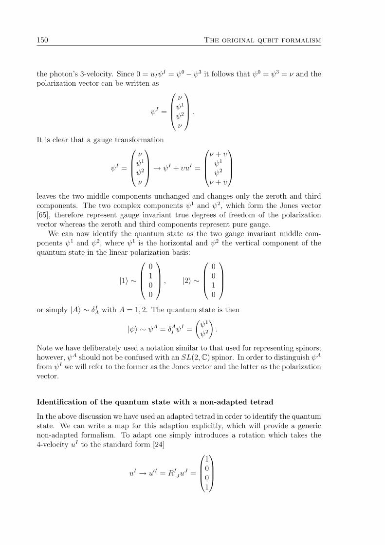
150 The original qubit formalism

the photon’s 3-velocity. Since 0 = uIψI = ψ0−ψ3 it follows that ψ0 = ψ3 = ν and the

polarization vector can be written as

ψI =

νψ1

ψ2

ν

.

It is clear that a gauge transformation

ψI =

νψ1

ψ2

ν

→ ψI + υuI =

ν + υψ1

ψ2

ν + υ

leaves the two middle components unchanged and changes only the zeroth and thirdcomponents. The two complex components ψ1 and ψ2, which form the Jones vector[65], therefore represent gauge invariant true degrees of freedom of the polarizationvector whereas the zeroth and third components represent pure gauge.

We can now identify the quantum state as the two gauge invariant middle com-ponents ψ1 and ψ2, where ψ1 is the horizontal and ψ2 the vertical component of thequantum state in the linear polarization basis:

|1〉 ∼

0100

, |2〉 ∼

0010

or simply |A〉 ∼ δIA with A = 1, 2. The quantum state is then

|ψ〉 ∼ ψA = δAI ψI =

(ψ1

ψ2

).

Note we have deliberately used a notation similar to that used for representing spinors;however, ψA should not be confused with an SL(2,C) spinor. In order to distinguish ψA

from ψI we will refer to the former as the Jones vector and the latter as the polarizationvector.

Identification of the quantum state with a non-adapted tetrad

In the above discussion we have used an adapted tetrad in order to identify the quantumstate. We can write a map for this adaption explicitly, which will provide a genericnon-adapted formalism. To adapt one simply introduces a rotation which takes the4-velocity uI to the standard form [24]

uI → u′I = RIJu

J =

1001

A.1 The quantum state 151

which results in the tetrad being aligned with the photon’s 3-velocity, as illustrated infigure A.1.

Such a rotation is explicitly given by

RIJ(u) = δI0δ

0J − rI rJ −

u3

u(P I

J + rI rJ)−√

1−(u3

u

)2

εIKJ0rK

where u3/u = uµeµ3/u = − cos θ is the angle between the direction of the photon and the

z-component of the tetrad, rI ≡ εIJ30uJ is the spatial axis of rotation with rI ≡ rI/|r|,

and P IJ ≡ δIJ − eI0e0

J is the projector onto the spacelike hypersurface orthogonal to thetetrad time axis (see Fig.A.1).

Figure A.1: The rotation R adapts the spacelike vectors of the tetrad ~ei so that thez-axis ~e3 is aligned to the 3-velocity of the photon ~u. A polarization vector is then in theplane spanned by R~e1 and R~e2.

It is important to stress that there are several other possible choices for this spatialrotation corresponding to different conventions for the linear polarization basis. Fur-thermore, the rotation matrix above becomes undefined for θ = π which is unavoidablefor topological reasons.

The rotation RIJ induces a linear polarization basis δAI R

IJ . We can now extract the

components of the quantum state expressed in this basis as

ψA = fAJ ψJ , with fAJ ≡ δAI R

IJ . (A.1)

It is clear that the specific linear polarization basis used here depends on how wehave adapted the tetrad to the velocity of the photon. However, regardless of whatconvention one chooses, the quantum state ψA is gauge invariant. Alternatively wecould think of the quantum state directly in terms of an equivalence class of polarizationvectors ψI ∼ ψI+υuI orthogonal to photon velocity uI . The advantage of this approachis that once one has developed a gauge invariant formalism one need not work with thecumbersome two component Jones vector, but instead can work solely with the gaugecovariant polarization vector ψI . This will be addressed below and in Section 6.1.2.

fAI from (A.1) turns out to provide a ‘diad’ frame: The two vectors f 1I and f 2

I spanthe two-dimensional space orthogonal to both the photon’s 4-velocity uI and the timecomponent of a tetrad etI . If we let f IA be the inverse of fAI we have that f IAf

AJ = δIJ and

f IAuI = f IAetI = 0. In fact, if we define wI to be a null vector defined by etI = 1

2(uI +wI)

[64], the vectors uI , wI , f1I and f 2

I span the full tangent space. This decomposition willbe useful when identifying unitary operations in Section 6.1.2.


A.2 The inner product

We must identify an inner product on the complex vector space for polarization so thatit can be promoted to a Hilbert space. In the analysis of the WKB limit we found thatjI = −√gkIϕ2ηJKψ

J ψK corresponded to a conserved 4-current which was physicallyinterpreted as a conserved probability density current. A natural inner product betweentwo polarization 4-vectors ψI and φJ is then given by

− ηIJ φIψJ . (A.2)

This form is clearly sesquilinear and positive definite for spacelike polarization vectors.1

Unlike the case for fermions, the inner product ηIJ is not explicitly dependent on thephoton 4-velocity. However, if we consider the gauge transformation ψI → ψI + υ1u

I1

and φI → φI + υ2uI2 it is clear that unless uI1 = uI2, i.e. kI1 ∝ kI2, the inner product

(4.40) is not gauge invariant. We conclude that two polarization vectors correspondingto two photons with non-parallel null velocities do not lie in the same Hilbert space.Furthermore, in order to be able to coherently add two polarization states it is alsonecessary to have kI1 = kI2, i.e. the two photons must have the same frequency. Undersuch conditions the inner product is both Lorentz invariant and gauge invariant. Withthe inner product (4.40) the complex vector space of polarization vectors is promotedto a Hilbert space which is notably labelled again with both position and 4-momentumpI = ~kI .

The above inner product (4.40) reduces to the standard inner product for a two-dimensional Hilbert space. This is best seen through the use of an adapted tetrad. Inan adapted frame the inner product of ψI = (ν, ψ1, ψ2, ν) with some other polarizationvector φI = (µ, φ1, φ2, µ) is given by

−ηIJ φIψJ = −µν + φ1ψ1 + φ2ψ

2 + µν = φ1ψ1 + φ2ψ

2 = 〈φ|ψ〉.

Thus, the standard inner product 〈φ|ψ〉 = φ1ψ1 + φ2ψ

2 is simply given by 〈φ|ψ〉 =−ηIJ φIψJ , where we associate

|ψ〉 ∼ ψI and 〈φ| ∼ −φI = −ηIJ φJ .

We can now work directly with the polarization 4-vector ψI which transforms in amanifestly Lorentz covariant and gauge covariant manner.

A.3 The relation to the Wigner formalism

The Wigner rotation W BA (k,Λ) on the quantum state represented by the Jones vector

which results from the transport of the polarization vector can be identified in the sameway as was done in §4.3.4 for fermions. Specifically, this is achieved by determining the

1There is no primed index for conjugate terms because the vector representation of the Lorentz

group is real.

A.3 The relation to the Wigner formalism 153

evolution of the Jones vector ψA that is induced by the transport of the quantum staterepresented by the polarization 4-vector ψI . Substituting ψI = f IBψ

B in the transport

equation (4.32), dψI

dλ+ uµω I

µ JψJ = βuI , and multiplying by fAI , we obtain

dψA

dλ= −

(uµeAI ω

Iµ Jf

JB + fAI

df IBdλ

)ψB + βfAI u

I . (A.3)

The last term is zero, as fAI is the diad frame defined to be orthogonal to uI . If we first

consider (A.3) in an adapted tetrad as in §4.4.4 we see that the derivativedfIBdλ

vanishesand the remaining term on the right-hand side can be simplified to

dψA

dλ= iuµωµ12σ

yABψ

B (A.4)

where we have made use of the antisymmetry of the spin-1 connection in order tointroduce the antisymmetric Pauli Y matrix σyAB.2 Eq.(A.4) is then clearly unitaryand helicity preserving as it is proportional to σyAB in the linear polarization basis.We can now readily identify the infinitesimal Wigner rotation as WA

B = iuµωµ12σyAB,

where the rotation angle is uµωµ12. In a non-adapted tetrad frame the map f IA = δJARIJ

can be seen to put (A.3) in the form (A.4) with a modified spin-1 connection ω′ Iµ J . TheWigner rotation for non-adapted tetrads is then

WAB = iuµ(R I

1 ∂µR2I +R I

1 ωJ

µI R2J)σyAB. (A.5)

A general Wigner rotation is understood as the composition of mapsWAB ≡ f IB(Λu)Λ J

I fAJ (u).

It is therefore no surprise that the transport of the polarization vector induces a Wignerrotation: The action of the gravitational field along a trajectory is simply a sequenceof infinitesimal Lorentz transformations which are given by uµω I

µ J (§4.1.2). The trans-port of the Jones vector is therefore described by a sequence of infinitesimal Wignerrotations given by (A.5). Notice that the Wigner rotation takes on a form which is notmanifestly Lorentz covariant. This is because the Wigner rotation describes a spatialrotation. This should be contrasted with the manifestly Lorentz covariant representa-tion in terms of parallel transported polarization vectors. Furthermore, after we havedeveloped a measurement formalism in section 6.1.2 it will become clear that there isno need to work with the cumbersome Wigner rotations.

2Note again that this should not be confused with the σ-matrices encountered when working with

spinors.


BNull Fermi-Walker transport

B.1 Jerk and non-geodesic motion

We have seen that the transport of qubits as massive fermions is governed by the spin-12

Fermi–Walker transport equation (§4.3.3). One might then expect that the transport ofqubits as polarization of photons along non-geodesic null-trajectories should similarlybe governed by a kind of Fermi–Walker transport. Transport of polarization vectors forthese non-geodesic null trajectories was developed by Castagnino [158–160]. However,these two proposals are mathematically distinct, and it is not clear to us which oneis the correct one. Furthermore, both of these proposals involve the ‘jerk’ along thepath, i.e. the time derivative of the acceleration, making the transport equation fornon-geodesic paths looks rather unpleasant.

It is easy to show that any transport of a polarization vector along a null pathmust involve three or more derivatives of the trajectory xµ(λ), i.e. involve one ormore derivative of the acceleration aµ(λ). From linearity and the requirement that thetransport reduces to the parallel transport for geodesics we deduce that the transport

must have the form DNFWφI

Dλ= DφI

Dλ+ T IJφ

J = 0. We now show that no such choiceof T IJ containing only the 4-velocity and the acceleration exists that preserves theorthogonality φIuI = 0 between the 4-velocity and the polarization vector. We havethat

0 =d

dλ(φIuI) =

D

Dλ(φIuI) =

DφI

DλuI + φIaI = −T IJuIφJ + φIaI .

However, if we now assume that the transport contains at most the second derivativeof xµ(λ) (i.e. the velocity uI and the acceleration aI) we deduce that T IJ = αuIuJ +βuIaJ + γaIuJ + δaIaJ . But since uIaI ≡ 0 we see that T IJuIφ

J ≡ 0 and we have thusdeduced that φIaI = 0 for all trajectories and all polarization vectors which is false.

155

156 Null Fermi-Walker transport

Therefore, we have a contradiction and we have to conclude that T IJ contains one ormore derivatives of the acceleration aI .

It is, however, not clear that it is appropriate to study transport of polarizationvectors along non-geodesic null trajectories. Physically, non-geodesic paths of photonscan only be achieved in the presence of a medium, in which case the photon trajectorieswill be timelike. In our approach a physically motivated way to obtain non-geodesictrajectories would be to introduce a medium in Maxwell’s equations through which thephoton propagates. Nevertheless, even without explicitly including a medium, it is easyto include optical elements such as mirrors, prisms, and other unitary transformationsas long as their effect on polarization can be considered separately to the effect oftransport through curved spacetime.

CRelationship between Wigner and Weyl

representations

We have now completely derived a relativistic covariant quantum information formal-ism. Specifically we have seen how to construct starting with the fundamental fieldequations the notion of a localized qubit in the relativistic context, the trajectoriesalong which they are transported and the governing transport equations. In the lightof the previous chapters we would now like to critically analyse the alternative treat-ment of the spin of a massive fermion as a representation of a qubit in the relativisticquantum information community. As we have already mentioned this treatment isbased on the Wigner representation which is related to the SL(2,C) representationused in this paper by adapting the reference frame to the particles four velocity. Inthis section we would like to compare the relationship between the Wigner and Weylrepresentations for a spin-1

2massive fermion.

157

158 Relationship between Wigner and Weyl representations

C.1 Relation to the Wigner representation

There are several important distinctions between the Wigner representation and theWeyl representation which we should make. Firstly in the Wigner representation thereis a natural tensor product between spin and momentum H = L2⊗C2, however in theWeyl representation we found that the Hilbert space for the spin degrees of freedomare in fact labelled by momentum we therefore have that H = ⊕pHp. The secondimportant distinction is in the transformation properties of the states under arbitraryLorentz transformations. In the Wigner representation one must determine the Wignerrotation matrix DA′A(W (Λ, P )) which essentially characterises the action of Lorentztransformations on the spin degrees of freedom. The rotation matrix has the peculiarfeature that the action of an arbitrary Lorentz transformation Λ on our states dependson the momentum. This is in contrast to the Weyl representation where the actionof Lorentz transformations are simply spin-1

2representations of Λ, Λ 1

2. Recall that

although the matrices Λ 12

are non-unitary, with the appropriate choice of inner productthe action of Λ 1

2on any state in our Hilbert space is indeed unitary in the sense that

they are norm preserving. Given that these two representations are very different it ishelpful to see precisely how they are related. To do this we will need to consider thequantized Dirac field.

C.1.1 Mathematical

In this section we would like to see the mathematical relationship between the Weylrepresentation presented in this thesis and the Wigner representation, to do this let usconsider the quantized Dirac field. The Dirac field can be expanded in a fourier seriesin terms of the annihilaion and creation operators for both fermions a(p, σ), a†(p, σ)and anti-fermions b(p, σ), b†(p, σ) which under fourier decomposition takes the form:

Ψ(x) =∑σ

∫dµ(p)

[u(p, σ)a(p, σ)e−ip·x + v(p, σ)b†(p, σ)e+ip·x

], (C.1)

or in the two component Weyl representation

φA(x) =∑σ

∫dµ(p)

[xA(p, σ)a(p, σ)e−ip·x + yA(p, σ)b†(p, σ)e+ip·x

], (C.2)

where dµ(p) = (2π)−3/2(2Ep)−1/2d3p is the Lorentz invariant measure. The relation-ship between four component dirac field and the Weyl 2-spinor is given by

u(p, σ) =

(xA(p, σ)

y†A′(p, σ)

).

In this context the Wigner state |p, σ〉 is simply defined to be a one particle exci-tation of the Dirac field and therefore we have

|p, σ〉 = (2π)3/2(2Ep)1/2a†(p, σ) |0〉

C.1 Relation to the Wigner representation 159

One can then show that in order for |p, σ〉 to have the appropriate transformation prop-erties as discussed in §3.2.1, the annihilation and creation operators must transformaccording to

U−1(Λ)a†(p, σ)U(Λ) = N(Λ, p)∑σ′

Dσσ′(W (Λ, p))a†(pΛ, σ′) (C.3)

where we have used the Lorentz invariance of the vacuum state |0〉. N(Λ, p) is anappropriate normalization constant and pΛ corresponds to the spatial components ofΛp [24]. Given that under an arbitrary Lorenz transformation the annihilation andcreation operators transform via a Wigner rotation we should understand them ascreating and annihilating states with rest-frame spin σ.

Consider now the one-particle wave functions ψ(x) and φA(x). They are defined as

ψ(x) ≡ 〈0| Ψ(x) |p, σ〉 = u(p, σ)e−ip·x and φA(x) ≡ 〈0| φA(x) |p, σ〉 = xA(p, σ)e−ip·x

A Lorentz transformation acting on |p, σ〉 in fact induces a spin-12

Lorentz transfor-mation on the one-particle wave functions. Therefore we can identify the Dirac wave-function φA(x) as a basis for the spatially localised quantum state presented in thisthesis. In order to see this it suffices to show that the transformation properties arethe same. To see this consider an arbitrary Lorentz transformation Λ acting on a Diracfield. In order for this to furnish a representation of the Lorentz group we must havethat

U−1(Λ)φA(x)U(Λ) = Λ BA φB(Λ−1x) (C.4)

Expanding the left hand side and using (C.3), we see that (C.4) is satisfied provided∑σ′

xA(p, σ′)D12

σσ′ = Λ BA xB(Λp, σ) (C.5)

Putting this all together let us now consider the transformation of the one-particlewave function under an arbitrary Lorentz transformation U(Λ) acting on |p, σ〉.

〈0| φA(x)U(Λ) |p, s;F 〉 = 〈0|U−1(Λ)φA(x)U(Λ) |p, σ〉 = Λ BA xB(p, σ)e−ip·Λ

−1x

where we have used (C.4), (C.5) and the Lorentz invariance of |0〉. Rearranging theright hand side

〈0| φA(x) |Λp, σ〉 = xA(Λp, σ)e−iΛp·x

which is in agreement with the transformation of the quantum state as found in §4.3.4.Note that we have expressed the wave-function as a function of the rest-frame spinσ, however given that this is indeed a basis for the quantum state we should identifyxA(p, σ) as belonging to Hp and we should remove the functional arguments (Λp, σ)which can be implicitly understood given the reference to the Hilbert space. That iswe have

xA(p, σ) = Λ BA xA = Λ 1

2χσ (C.6)

Where χσ corresponds to the spin components σ in the rest-frame, and correspondsto the restframe spin which as we have already shown has the same transformationproperties as the Wigner representation (4.21).

160 Relationship between Wigner and Weyl representations

(a) (b)

Figure C.1: Comparison of the action of Lorentz transformations between the (a) Weyland (b) Wigner representations. (a) Lorentz transformations takes a state ψA ∈ Hp1 to anew state Λ B

A ψB ∈ Hp2 . (b) Lorentz transformations correspond to actions which preservethe standard momentum k.

C.1.2 Geometric

We have shown the clear mathematical relationship between these two representations.It is perhaps helpful to give a clearer geometric picture of this mathematical relationshipbetween these two different representations. With in the Weyl representation a Lorentztransformation simply acts via a spin-1

2Lorentz transformation and one adapts the in-

ner product with the four momentum of the qubit. This is illustrated in Fig C.1(a).However in he Wigner representation instead of adapting the inner product one choosesa standard momentum k and actions of the Lorentz group on the Hilbert space for spinH = C2 are defined as those which leave k invariant, that is W (Λ, p) = L−1(Λp)ΛL(p).For equal to the rest frame momentum k = (1, 0, 0, 0), this is illustrated in Fig C.1(b).As we showed in §4.3.4 the Weyl representation reduces to that of the Wigner repre-sentation by simply re-expressing the action of Lorentz transformations on ψA as thoseacting on the rest-frame spin ψA. Given that the choice of the standard momentum kis arbitrary one should strictly speaking also index the spin Hilbert space with k, i.e.H = C2

k=p, where p denotes the rest-frame momentum .

References

[1] A. Ashtekar. New variables for classical and quantum gravity. Phys. Rev. Lett.57, 2244 (1986). 1

[2] B. S. DeWitt. Quantum theory of gravity. i. the canonical theory. Phys. Rev.160, 1113 (1967). 105

[3] P. G. Bergmann. Hamilton-jacobi and schrodinger theory in theories with first-class hamiltonian constraints. Phys. Rev. 144, 1078 (1966).

[4] C. Rovelli. Quantum Gravity. Cambridge Monographs on Mathematical Physics(Cambridge University Press, 2007). 1

[5] J. D. Bekenstein. Black holes and entropy. Phys. Rev. D 7, 2333 (1973). 1

[6] S. Hawking. Particle creation by black holes. Commun. Math. Phys. 43, 199(1975). 10.1007/BF02345020. 1

[7] A. Einstein. Die Feldgleichungen der Gravitation. Sitzungsberichte der Preussis-chen Akademie der Wissenschaften zu Berlin pp. 844–847 (1915). 1

[8] D. Hilbert. Grundlagen der physik, erste mitteilung, vorgelegtin der sitzung. Vom 20, November 1915. English translationhttp://www.springerlink.com/content/t2681418480nq841 . 1

[9] N. D. Birrell and P. C. W. Davies. Quantum Fields in Curved Space (CambridgeMonographs on Mathematical Physics) (Cambridge University Press, 1984). 7,30, 32

[10] R. M. Wald. Quantum Field Theory in Curved Spacetime and Black Hole Ther-modynamics (University Of Chicago Press, 1994), 1 ed. 30

[11] V. Mukhanov and S. Winitzki. Introduction to Quantum Effects in Gravity (Cam-bridge University Press, 2007). 7

[12] P. M. Alsing, I. Fuentes-Schuller, R. B. Mann, and T. E. Tessier. Entanglementof dirac fields in noninertial frames. Phys. Rev. A 74, 032326 (2006). 7

161

http://www.springerlink.com/content/t2681418480nq841

162 References

[13] I. Fuentes, R. B. Mann, E. Martın-Martınez, and S. Moradi. Entanglement ofdirac fields in an expanding spacetime. Phys. Rev. D 82, 045030 (2010). 22

[14] E. Martın-Martınez, I. Fuentes, and R. B. Mann. Using berry’s phase to detectthe unruh effect at lower accelerations. Phys. Rev. Lett. 107, 131301 (2011).

[15] J. Louko and A. Satz. How often does the unruh–dewitt detector click? regular-ization by a spatial profile. Classical and Quantum Gravity 23(22), 6321 (2006).32

[16] E. Martın-Martınez. Relativistic quantum information: developments in quantuminformation in general relativistic scenarios. arXiv:1106.0280v1 (2011). arXiv:

1106.0280. 7

[17] H. Terashima and M. Ueda. Einstein-podolsky-rosen correlation in a gravitationalfield. Phys. Rev. A 69, 032113 (2004). 7, 8, 22, 23, 33, 42, 43, 97

[18] P. M. Alsing, G. J. Stephenson Jr, and K. P. Spin-induced non-geodesic motion,gyroscopic precession, wigner rotation and epr correlations of massive spin 1/2particles in a gravitational field (2009). arXiv:0902.1396v1. 7, 8, 22, 97

[19] J. L. Pienaar, C. R. Myers, and T. C. Ralph. Space-time qubits. Phys. Rev. A84, 022315 (2011). 7

[20] A. Brodutch, T. F. Demarie, and D. R. Terno. Photon polarization and geometricphase in general relativity. Phys. Rev. D 84, 104043 (2011). 7, 101

[21] A. Peres and D. R. Terno. Quantum information and relativity theory. Rev.Mod. Phys. 76, 93 (2004). 7, 8, 22, 54, 90, 95, 99

[22] E. Wigner. On unitary representations of the inhomogeneous lorentz group. Ann.Math. 40(1), 149 (1939). 8, 19

[23] Y. S. Kim and M. E. Noz. Theory and applications of the Poincare group (Reidel; Sold and distributed in the U.S.A. and Canada by Kluwer Academic Publishers,Dordrecht, Holland ; Boston : Hingham, MA :, 1986). 8, 33

[24] S. Weinberg. The Quantum Theory of Fields, Vol. 1: Foundations (CambridgeUniversity Press, 1995), 1 ed. 8, 21, 42, 43, 53, 150, 159

[25] A. Peres, P. F. Scudo, and D. R. Terno. Quantum entropy and special relativity.Phys. Rev. Lett. 88, 230402 (2002). 8, 22, 90, 95, 99

[26] A. Peres and D. R. Terno. Quantum information and special relativity. Int. J.Quant. Info. 1, 225 (2003). arXiv:quant-ph/0301065. 22, 95

[27] S. D. Bartlett and D. R. Terno. Relativistically invariant quantum information.Phys. Rev. A 71, 012302 (2005). 8, 22, 95, 99

arXiv:1106.0280

arXiv:1106.0280

arXiv:0902.1396v1

arXiv:quant-ph/0301065

References 163

[28] L. Stodolsky. Matter and light wave interferometry in gravitational fields. GeneralRelativity and Gravitation 11(6), 391 (1979). 8, 62

[29] P. M. Alsing, J. C. Evans, and K. K. Nandi. The phase of a quantum mechanicalparticle in curved spacetime. Gen. Relativ. Gravit. 33, 1459 (2000). arXiv:

gr-qc/0010065. 62

[30] J. Anandan. Gravitational and rotational effects in quantum interference. Phys.Rev. D 15, 1448 (1977). 9, 56, 66, 67, 68, 69

[31] J. Audretsch and C. Lammerzahl. New inertial and gravitational effects mademeasurable by atomic beam interferometry. Appl. Phys. B 54, 351 (1992).10.1007/BF00325379. 56, 66, 68, 69

[32] J. J. Sakurai. Modern Quantum Mechanics (Revised Edition) (Addison Wesley,1993), rev sub ed. 56, 66, 68

[33] S. A. Werner. Gravitational, rotational and topological quantum phase shifts inneutron interferometry. Classical and Quantum Gravity 11(6A), A207 (1994).8, 67, 68

[34] R. Colella, A. W. Overhauser, and S. A. Werner. Observation of gravitationallyinduced quantum interference. Phys. Rev. Lett. 34, 1472 (1975). 9, 56, 66, 68,69

[35] P. D. Mannheim. Classical underpinnings of gravitationally induced quantuminterference. Phys. Rev. A 57, 1260 (1998). 9, 63

[36] K. Varju and L. H. Ryder. General relativistic treatment of the colella-overhauser-werner experiment on neutron interference in a gravitational field. Am. J. Phys.68(5), 404 (2000). 9, 56, 66, 67, 68

[37] S. Carroll. Spacetime and Geometry: An Introduction to General Relativity (Ben-jamin Cummings, 2003). 11

[38] R. M. Wald. General Relativity (University Of Chicago Press, 1984), 1 ed. 16,18

[39] D. Bailin and A. Love. Supersymmetric Gauge Field Theory and String Theory(Taylor & Francis, 1994), 1 ed. 16, 17, 43, 74

[40] R. Penrose and W. Rindler. Spinors and Space-Time: Volume 1, Two-Spinor Cal-culus and Relativistic Fields (Cambridge Monographs on Mathematical Physics)(Cambridge University Press, 1987). 16, 50

[41] P. Caban and J. Rembielinski. Photon polarization and wigner’s little group.Phys. Rev. A 68, 042107 (2003). 21, 22, 54

[42] M. Czachor. Einstein-podolsky-rosen-bohm experiment with relativistic massiveparticles. Phys. Rev. A 55, 72 (1997). 22, 83, 90, 91, 92

arXiv:gr-qc/0010065

arXiv:gr-qc/0010065

164 References

[43] P. M. Alsing and G. J. Stephenson Jr. The wigner rotation for photons in anarbitrary gravitational field (2009). arXiv:0902.1399v1. 22

[44] T. D. Newton and E. P. Wigner. Localized states for elementary systems. Rev.Mod. Phys. 21, 400 (1949). 29

[45] G. C. Hegerfeldt. Remark on causality and particle localization. Phys. Rev. D10, 3320 (1974). 29, 48

[46] I. Bialynicki-Birula. Exponential localization of photons. Phys. Rev. Lett. 80,5247 (1998). 29, 48

[47] S. Weinberg. Gravitation and Cosmology: Principles and Applications of theGeneral Theory of Relativity (Wiley, 1972), 1 ed. 30, 39

[48] M. E. Peskin and D. V. Schroeder. An Introduction To Quantum Field Theory(Frontiers in Physics) (Westview Press, 1995). 31, 87

[49] V. A. Bordovitsyn and I. M. Ternov. Synchrotron Radiation Theory and itsDevelopment: in Memory of I.M. Ternov (World Scientific, 1999). 31

[50] D. Melrose. Quantum Plasmadynamics: Unmagnetized Plasmas (Lecture Notesin Physics) (v. 1) (Springer, 2007), 1 ed.

[51] D. Melrose. Quantum Plasmadynamics: Magnetized Plasmas (Springer, 2010),1 ed. 31, 32

[52] W. G. Unruh. Notes on black-hole evaporation. Phys. Rev. D 14, 870 (1976). 32

[53] E. T. Akhmedov and D. Singleton. On the relation between unruh and sokolov–ternov effects. Int. J. Mod. Phys. A 22, 4797 (2007). 32

[54] H. K. Dreiner, H. E. Haber, and S. P. Martin. Two-component spinor techniquesand feynman rules for quantum field theory and supersymmetry. Phys. Rept.494, 1 (2010). 33, 36, 41, 42, 73

[55] M. Nakahara. Geometry, Topology and Physics (Taylor & Francis, 2003), 2 ed.34

[56] J. J. Sakurai. Advanced Quantum Mechanics (Addison-Wesley, Reading, Mas-sachusetts, 1980). 34, 87

[57] J. Audretsch. Dirac electron in space-times with torsion: Spinor propagation,spin precession, and nongeodesic orbits. Phys. Rev. D 24, 1470 (1981). 35

[58] J. and Anandan. Topological and geometrical phases due to gravitational fieldwith curvature and torsion. Physics Letters A 195(5-6), 284 (1994).

[59] P. G. Bergmann, (ed. ), V. de Sabbata, (ed. ), G. T. Gillies, (ed. ), and P. I.Pronin, (ed. ). Spin in gravity: Is it possible to give an experimental basis totorsion? (World Scientific, 1997). 35, 47, 101

arXiv:0902.1399v1

References 165

[60] A. Peres. Quantum Theory: Concepts and Methods (Fundamental Theories ofPhysics) (Springer, 1993). 37, 85, 86

[61] C. W. Misner, K. S. Thorne, and J. A. Wheeler. Gravitation (Physics Series)(W. H. Freeman, 1973), 1 ed. 38, 39, 44, 45, 67, 86

[62] N. Woodhouse. Special Relativity (Springer, Berlin, 1992). 44, 45

[63] W. Rindler. Introduction to Special Relativity (Oxford University Press, USA,1991). 44, 62, 67

[64] E. Poisson. A Relativist’s Toolkit : The Mathematics of Black-Hole Mechanics(Cambridge University Press, 2004). 48, 50, 151

[65] E. Hecht. Optics (Addison-Wesley, 2002), 4 ed. 51, 150

[66] I. Bengtsson and K. Zyczkowski. Geometry of Quantum States: An Introductionto Quantum Entanglement (Cambridge University Press, 2008). 59

[67] M. V. Berry. Quantal Phase Factors Accompanying Adiabatic Changes. Pro-ceedings of the Royal Society of London. Series A, Mathematical and PhysicalSciences 392(1802), 45 (1984). 65

[68] C. K. Hong, Z. Y. Ou, and L. Mandel. Measurement of subpicosecond timeintervals between two photons by interference. Phys. Rev. Lett. 59, 2044 (1987).79

[69] S. D. Bartlett, T. Rudolph, and R. W. Spekkens. Reference frames, superselectionrules, and quantum information. Rev. Mod. Phys. 79, 555 (2007). 80

[70] T. Rudolph and B. C. Sanders. Requirement of optical coherence for continuous-variable quantum teleportation. Phys. Rev. Lett. 87, 077903 (2001). 101

[71] S. D. Bartlett, T. Rudolph, and R. W. Spekkens. Dialogue concerning two viewson quantum coherence: Factist and fictionist. Int. J. Quantum Inf. 4, 17 (2006).101

[72] S. D. Bartlett, T. Rudolph, R. W. Spekkens, and P. S. Turner. Quantum com-munication using a bounded-size quantum reference frame. N. J. Phys. 11(6),063013 (2009). 80

[73] M. C. Palmer, M. Takahashi, and H. F. Westman. Localized qubits in curvedspacetimes. Annals of Physics 327(4), 1078 (2012). 83, 84, 86, 87, 88, 149

[74] L. L. Foldy and S. A. Wouthuysen. On the dirac theory of spin 1/2 particles andits non-relativistic limit. Phys. Rev. 78, 29 (1950). 83

[75] F. W. Hehl and W.-T. Ni. Inertial effects of a dirac particle. Phys. Rev. D 42,2045 (1990).

166 References

[76] L. H. Ryder. Relativistic treatment of inertial spin effects. Journal of Physics AMathematical General 31, 2465 (1998).

[77] L. H. Ryder. Relativistic Spin Operator for Dirac Particles. General Relativityand Gravitation 31, 775 (1999).

[78] B. Mashhoon. On the coupling of intrinsic spin with the rotation of the earth.Physics Letters A 198, 9 (1995). 83

[79] D. R. Terno. Two roles of relativistic spin operators. Phys. Rev. A 67, 014102(2003). 83, 90, 91, 92

[80] P. Caban and J. Rembielinski. Lorentz-covariant reduced spin density matrix andeinstein-podolsky-rosen-bohm correlations. Phys. Rev. A 72, 012103 (2005). 90

[81] P. Caban and J. Rembielinski. Einstein-podolsky-rosen correlations of dirac par-ticles - quantum field theory approach. Phys. Rev. A 74, 042103 (2006).

[82] N. Friis, R. A. Bertlmann, M. Huber, and B. C. Hiesmayr. Relativistic entangle-ment of two massive particles. Phys. Rev. A 81, 042114 (2010). 90, 95, 99

[83] M. Czachor and M. Wilczewski. Relativistic bennett-brassard cryptographicscheme, relativistic errors, and how to correct them. Phys. Rev. A 68, 010302(2003). 83

[84] P. L. Saldanha and V. Vedral. Physical interpretation of the wigner rotationsand its implications for relativistic quantum information. New Journal of Physics14(2), 023041 (2012). 83, 86, 94

[85] L. E. Ballentine. Quantum Mechanics: A Modern Development (World ScientificPublishing Company, 1998). 86

[86] A. G. S. Landulfo and G. E. A. Matsas. Influence of detector motion in bellinequalities with entangled fermions. Phys. Rev. A 79, 044103 (2009). 90

[87] N. Bogoliubov and D. Shirkov. Introduction to axiomatic quantum field theory(Wiley-Interscience, 1980). 92

[88] R. M. Gingrich and C. Adami. Quantum entanglement of moving bodies. Phys.Rev. Lett. 89, 270402 (2002). 95, 99

[89] T. Choi. Relativistic spin operator and lorentz transformation of spin state of amassive dirac particle. arXiv:1209.4440 (2012). 95

[90] D. R. Terno. Quantum Information Processing: From Theory to Experiment,edited D.G. Angelakis et al., pp. 61–86 (IOP Press, 2006).

[91] M. Czachor. Comment on “quantum entropy and special relativity”. Phys. Rev.Lett. 94, 078901 (2005). 95, 99

References 167

[92] R. Jozsa, D. S. Abrams, J. P. Dowling, and C. P. Williams. Quantum clocksynchronization based on shared prior entanglement. Phys. Rev. Lett. 85, 2010(2000). 101

[93] V. Giovannetti, S. Lloyd, and L. Maccone. Quantum-enhanced positioning andclock synchronization. Nature 412, 417 (2001). arXiv:quant-ph/0103006.

[94] M. de Burgh and S. D. Bartlett. Quantum methods for clock synchronization:Beating the standard quantum limit without entanglement. Phys. Rev. A 72,042301 (2005). 101

[95] S. J. Jones, H. M. Wiseman, S. D. Bartlett, J. A. Vaccaro, and D. T. Pope. En-tanglement and symmetry: A case study in superselection rules, reference frames,and beyond. Phys. Rev. A 74, 062313 (2006). 101

[96] S. D. Bartlett, A. C. Doherty, R. W. Spekkens, and H. M. Wiseman. Entangle-ment under restricted operations: Analogy to mixed-state entanglement. Phys.Rev. A 73, 022311 (2006). 101

[97] C. W. F. Everitt, D. B. DeBra, B. W. Parkinson, J. P. Turneaure, J. W. Conklin,M. I. Heifetz, G. M. Keiser, A. S. Silbergleit, T. Holmes, J. Kolodziejczak, M. Al-Meshari, J. C. Mester, B. Muhlfelder, V. G. Solomonik, K. Stahl, P. W. Worden,W. Bencze, S. Buchman, B. Clarke, A. Al-Jadaan, H. Al-Jibreen, J. Li, J. A.Lipa, J. M. Lockhart, B. Al-Suwaidan, M. Taber, and S. Wang. Gravity probeb: Final results of a space experiment to test general relativity. Phys. Rev. Lett.106, 221101 (2011). 101

[98] A. Brodutch and D. R. Terno. Polarization rotation, reference frames, and mach’sprinciple. Phys. Rev. D 84, 121501 (2011). 101

[99] A. M. Childs, J. Preskill, and J. Renes. Quantum information and precisionmeasurement. J. Mod. Opt. 47, 155 (2000). 101

[100] G. M. D’Ariano, P. Lo Presti, and M. G. A. Paris. Using entanglement improvesthe precision of quantum measurements. Phys. Rev. Lett. 87, 270404 (2001).

[101] J. Preskill. Quantum information and physics: some future directions. J. Mod.Opt. 47, 127 (2000).

[102] V. Giovannetti, S. Lloyd, and L. Maccone. Quantum-enhanced measurements:beating the standard quantum limit. Science 306, 1330 (2004).

[103] G. Chiribella, G. M. D’Ariano, and M. F. Sacchi. Optimal estimation of grouptransformations using entanglement. Phys. Rev. A 72, 042338 (2005).

[104] G. Y. Xiang, B. L. Higgins, D. W. Berry, H. M. Wiseman, and G. J. Pryde.Entanglement-enhanced measurement of a completely unknown optical phase. Na-ture Photonics 5, 43 (2011). arXiv:quant-ph/1003.5213. 101

arXiv:quant-ph/0103006

arXiv:quant-ph/1003.5213

168 References

[105] J. Barbour. The End of Time: The Next Revolution in Physics (Weidenfeld andNicholson, 1999). 105, 110

[106] J. Barbour. The Discovery of Dynamics: A Study from a Machian Point of Viewof the Discovery and the Structure of Dynamical Theories (Oxford UniversityPress, 2001).

[107] J. Barbour. The nature of time. arXiv:0903.3489 (2009). 108, 110

[108] H. R. Brown. Physical relativity: Space-Time Structure From a Dynamical Per-spective (Clarendon, Oxford, 2005), 1. publ. ed. 105, 106, 108, 110

[109] E. Anderson. The problem of time in quantum gravity (2010). arXiv:1009.2157.105

[110] C. Kiefer. Does time exist in quantum gravity? (2009). arXiv:0909.3767.

[111] L. Smolin. Unimodular loop quantum gravity and the problems of time (2010).arXiv:1008.1759.

[112] L. Smolin. How far are we from the quantum theory of gravity? (2003). arXiv:hep-th/0303185. 105

[113] J. Barbour. The definition of machs principle. Foundations of Physics 40, 1263(2010). 10.1007/s10701-010-9490-7. 105

[114] I. Newton and F. Cajori. Sir Isaac Newton’s Mathematical Principles of NaturalPhilosophy and His System of the World: The system of the world. No. v. 1 inSir Isaac Newtons mathematical principles on natural philosophy and his systemof the world (University of California Press, 1962). 105, 106, 108, 112

[115] A. Einstein. On the Electrodynamics of Moving Bodies. Annalen der Physik 17(1905). 106

[116] A. Einstein. Autobiographical Notes in Albert Einstein: Philosopher-Scientist P.A. Schilpp (ed.), Library of Living Philosophers, vol. III (Cambridge UnicersityPress, 1970). 106

[117] C. Audoin and B. Guinot. The Measurement of Time: Time, Frequency and theAtomic Clock (Cambridge University Press, 2001). 109, 118, 122

[118] A. Jones. Splitting The Second: The Story of Atomic Time (Taylor & Francis,2010). 109, 110

[119] R. Rynasiewicz. By their properties, causes and effects: Newton’s scholium ontime, space, place and motioni. the text. Studies in History and Philosophy ofScience Part A 26(1), 133 (1995). 112

[120] J. Barbour and S. Echols. Absolute and relative motion. Manuscript (c2003). 117

arXiv:1009.2157

arXiv:0909.3767

arXiv:1008.1759

arXiv:hep-th/0303185

arXiv:hep-th/0303185

References 169

[121] J. B. Barbour and B. Bertotti. Mach’s Principle and the Structure of DynamicalTheories. Proceedings of the Royal Society of London. A. Mathematical andPhysical Sciences 382(1783), 295 (1982). 117

[122] P. Ehrenfest. Bemerkung uber die angenaherte Gultigkeit der klassischenMechanik innerhalb der Quantenmechanik. Zeitschrift fur Physik A Hadronsand Nuclei 45(7), 455 (1927). 120

[123] E. Joos. Decoherence and the Appearance of a Classical World in QuantumTheory. Physics and astronomy online library (Springer, 2003). 120

[124] D. N. Page and W. K. Wootters. Evolution without evolution: Dynamics describedby stationary observables. Phys. Rev. D 27, 2885 (1983). 121

[125] J. C. Arce. Unification of the conditional probability and semiclassical interpre-tations for the problem of time in quantum theory. Phys. Rev. A 85, 042108(2012).

[126] R. Gambini, R. A. Porto, J. Pullin, and S. Torterolo. Conditional probabilitieswith dirac observables and the problem of time in quantum gravity. Phys. Rev.D 79, 041501 (2009).

[127] C. Rovelli. Time in quantum gravity: An hypothesis. Phys. Rev. D 43, 442(1991).

[128] R. Gambini and J. Pullin. Relational physics with real rods and clocks and themeasurement problem of quantum mechanics. Foundations of Physics 37(7), 1074(2007). 121

[129] H. Westman and S. Sonego. Coordinates, observables and symmetry in relativity.Annals of Physics 324(8), 1585 (2009). 122

[130] I. L. Chuang and M. A. Nielsen. Prescription for experimental determination ofthe dynamics of a quantum black box. J. Mod. Opt. 44, 2455 (1997). 125

[131] D. F. V. James, P. G. Kwiat, W. J. Munro, and A. G. White. Measurement ofqubits. Phys. Rev. A 64, 052312 (2001). 125, 136, 139

[132] C. F. Roos, G. P. T. Lancaster, M. Riebe, H. Haffner, W. Hansel, S. Gulde,C. Becher, J. Eschner, F. Schmidt-Kaler, and R. Blatt. Bell states of atoms withultralong lifetimes and their tomographic state analysis. Phys. Rev. Lett. 92,220402 (2004). 125

[133] V. V. Dobrovitski, G. de Lange, D. Riste, and R. Hanson. Bootstrap tomographyof the pulses for quantum control. Phys. Rev. Lett. 105, 077601 (2010). 126

[134] A. M. Branczyk, D. H. Mahler, L. A. Rozema, A. Darabi, A. M. Steinberg, andD. F. V. James. Self-calibrating quantum state tomography. New J. Phys. 14(8),085003 (2012).

170 References

[135] S. T. Merkel, J. M. Gambetta, J. A. Smolin, S. Poletto, A. D. Corcoles, B. R.Johnson, C. A. Ryan, and M. Steffen. Self-Consistent Quantum Process Tomog-raphy. arXiv:1211.0322 (2012). 1211.0322. 140

[136] D. Rosset, R. Ferretti-Schobitz, J.-D. Bancal, N. Gisin, and Y.-C. Liang. Im-perfect measurement settings: Implications for quantum state tomography andentanglement witnesses. Phys. Rev. A 86, 062325 (2012).

[137] T. Moroder, M. Kleinmann, P. Schindler, T. Monz, O. Guhne, and R. Blatt.Certifying systematic errors in quantum experiments. Phys. Rev. Lett. 110,180401 (2013). 126

[138] J. R. Petta, A. C. Johnson, J. M. Taylor, E. A. Laird, A. Yacoby, M. D. Lukin,C. M. Marcus, M. P. Hanson, and A. C. Gossard. Coherent manipulation ofcoupled electron spins in semiconductor quantum dots. Science 309(5744), 2180(2005). 126

[139] J. M. Taylor, J. R. Petta, A. C. Johnson, A. Yacoby, C. M. Marcus, and M. D.Lukin. Relaxation, dephasing, and quantum control of electron spins in doublequantum dots. Phys. Rev. B 76, 035315 (2007).

[140] S. Foletti, H. Bluhm, D. Mahalu, V. Umansky, and A. Yacoby. Universal quantumcontrol of two-electron spin quantum bits using dynamic nuclear polarization. Nat.Phys. 5(12), 903 (2009). xv, 126, 127, 129, 130, 132, 136

[141] M. D. Shulman, O. E. Dial, S. P. Harvey, H. Bluhm, V. Umansky, and A. Yacoby.Demonstration of entanglement of electrostatically coupled singlet-triplet qubits.Science 336(6078), 202 (2012). 126, 134

[142] K. C. Nowack, M. Shafiei, M. Laforest, G. E. D. K. Prawiroatmodjo, L. R.Schreiber, C. Reichl, W. Wegscheider, and L. M. K. Vandersypen. Single-shotcorrelations and two-qubit gate of solid-state spins. Science 333(6047), 1269(2011). 126

[143] R. Brunner, Y. S. Shin, T. Obata, M. Pioro-Ladriere, T. Kubo, K. Yoshida,T. Taniyama, Y. Tokura, and S. Tarucha. Two-Qubit Gate of Combined Single-Spin Rotation and Interdot Spin Exchange in a Double Quantum Dot. Phys. Rev.Lett. 107(14), 146801 (2011).

[144] E. A. Laird, J. M. Taylor, D. P. DiVincenzo, C. M. Marcus, M. P. Hanson, andA. C. Gossard. Coherent spin manipulation in an exchange-only qubit. Phys.Rev. B 82, 075403 (2010).

[145] J. Medford, J. Beil, J. M. Taylor, S. D. Bartlett, A. C. Doherty, E. I. Rashba,D. P. DiVincenzo, H. Lu, A. C. Gossard, and C. M. Marcus. Self-consistent mea-surement and state tomography of an exchange-only spin qubit. arXiv:1302.1933(2013). 126

1211.0322

References 171

[146] J. Medford, J. Beil, J. M. Taylor, E. I. Rashba, , H. Lu, A. C. Gossard, and C. M.Marcus. The resonant exchange qubit. arXiv:1304.3413 (2013). 126

[147] J. M. Chow, J. M. Gambetta, A. D. Corcoles, S. T. Merkel, J. A. Smolin,C. Rigetti, S. Poletto, G. A. Keefe, M. B. Rothwell, J. R. Rozen, M. B. Ketchen,and M. Steffen. Universal quantum gate set approaching fault-tolerant thresholdswith superconducting qubits. Phys. Rev. Lett. 109, 060501 (2012). 126

[148] L. DiCarlo, J. M. Chow, J. M. Gambetta, L. S. Bishop, B. R. Johnson, D. I.Schuster, J. Majer, A. Blais, L. Frunzio, S. M. Girvin, and R. J. Schoelkopf.Demonstration of two-qubit algorithms with a superconducting quantum processor.Nature 460(7252), 240 (2009).

[149] R. C. Bialczak, M. Ansmann, M. Hofheinz, E. Lucero, M. Neeley, A. D.O’Connell, D. Sank, H. Wang, J. Wenner, M. Steffen, A. N. Cleland, and J. M.Martinis. Quantum process tomography of a universal entangling gate imple-mented with Josephson phase qubits. Nat. Phys. 6(6), 409 (2010). 126

[150] N. Rohling and G. Burkard. Tomography scheme for two spin-1/2 qubits in adouble quantum dot. arXiv:1304.2954 (2013). 126

[151] M. Nielsen and I. Chuang. Quantum Computation and Quantum Information(Cambridge University Press, Cambridge, 2000), 10 ed. 126, 138

[152] C. Barthel, D. J. Reilly, C. M. Marcus, M. P. Hanson, and A. C. Gossard. Rapidsingle-shot measurement of a singlet-triplet qubit. Phys. Rev. Lett. 103, 160503(2009). 128

[153] J. L. O’Brien, G. J. Pryde, A. Gilchrist, D. F. V. James, N. K. Langford, T. C.Ralph, and A. G. White. Quantum process tomography of a controlled-not gate.Phys. Rev. Lett. 93, 080502 (2004). 139

[154] D. P. Bertsekas. Constrained Optimization and Lagrange Multiplier Methods(Athena Scientific, Belmont, Massachusetts, 1996), 1 ed. 139

[155] T. Yamamoto, M. Neeley, E. Lucero, R. C. Bialczak, J. Kelly, M. Lenander,M. Mariantoni, A. D. O’Connell, D. Sank, H. Wang, M. Weides, J. Wenner,Y. Yin, A. N. Cleland, and J. M. Martinis. Quantum process tomography of two-qubit controlled-z and controlled-not gates using superconducting phase qubits.Phys. Rev. B 82, 184515 (2010). 139

[156] R. Penrose. On Gravity’s role in Quantum State Reduction. General Relativityand Gravitation 28(5), 581 (1996). 146, 147

[157] M. R. Vanner, I. Pikovski, M. S. Kim, C. Brukner, K. Hammerer, G. J. Milburn,and M. Aspelmeyer. Pulsed quantum optomechanics (2010). 1011.0879. 147

[158] M. Castagnino. Rend. Mat. 24, 438 (1965). Original paper, in Italian. 155

1011.0879

172 References

[159] D. Bini, A. Geralico, and R. T. Jantzen. Frenet–serret formalism for null worldlines. Classical and Quantum Gravity 23(11), 3963 (2006).

[160] J. Samuel and R. Nityananda. Transport along null curves. J. Phys. A 33(14),2895 (2000). 155

Documents

Copyright and use of this thesis - University of Sydney