Corruption, Military Spending and Growth

d’Agostino G.*, Dunne J. P.**, Pieroni L.***

*University of Rome III (Italy), and University of the West of England (UK)

**University of the West of England (UK), and University of Cape Town (RSA)

***University of Perugia (Italy)

Abstract

This paper considers the complementary effect of corruption and military spendingon economic growth, analyzing both the impact of public spending and the allocationof resources between categories of public spending. The non-linearities emerged fromthe endogenous growth model are due to the links among public spending components,corruption and economic growth. The main findings of the empirical results confirmthe expectation that corruption and military burden lower GDP per capita growthrate. They also suggest that omitting the complementarity effect between militaryspending and corruption the impact on economic performance is underestimated.

Keywords : corruption, military spending, development economics

JEL Classification : O57, H5, D73

1

1 Introduction

Allegations of corruption in the military sector are neither infrequent nor unexpected. It

is argued that the limited competition in the defence sector leads to a relatively high level of

informal contracts and to rent-seeking activities, providing fertile ground for the growth of

corrupt practices. This can have lead to an increase in the cost of military activities and their

burden on the economies rent seeking in the military sector and may crowd out productive

investment in the private second, meaning there are both direct and indirect effects.

We follow the theoretical suggestions of the endogenous growth model originally devel-

oped by Barro (1990) and propose as explanatory key decisions of the model the comple-

mentary effects that arises between private and public sectors and the detrimental effects of

corruption. In our model the government expenditure for military sector and public invest-

ment are defined as potential productive inputs, with different productivity, and corruption

impact on the long run economic growth. The model also incorporates the inefficiencies

of the corruption linked services provided by the public sector (red tape and bureaucratic

corruption), although it does not affect long run growth.

Our research is related to a number of empirical papers that test if the more corruption

enhances the level of military spending (and vice-versa), implying that they are complements

in constraining the economic growth (Mauro, 1995, 1998; Aizenman and Glick, 2003) . Our

work is closed in the spirit to Tanzi (1998) Gupta et al. (2000) who argued that produc-

tive public investments is scaled down in countries with widespread corruption in favour of

government expenditure less verifiable such as the military one.

This paper contributes in this literature in two ways. First, we test if the magnitude

of corruption is associated with a larger size of expenditure of the military sector (as well

as of government spending in investments) and how this externality leads to cut economic

growth. We focus our attention on military-corruption link with economic performance.

These effects of corruption seem particularly relevant when they are associated with higher

shares of military spending in GDP. The confidentialness of some military operations and

privateness in the control of natural resources in developing countries makes difficult any

provisional analysis of costs increasing the discretionary power of the bureaucratic lobby

2

and the corruption level of the public officer (Gupta, 2000). For this reason, we address the

analysis specifically to a large sample of African countries.

Furthermore, we motivate our analysis by estimating from empirical model three types

of elasticities that are able to account for military spending/corruption relationship in the

use of policy analyses (Lee, 2006): i) direct elasticities that arise from the estimations of

the parameters of the model; ii) indirect elasticities that measure the interaction between

corruption and components of government spending, and iii) total elasticities as a sum of

the elasticity i) and ii).

The empirical results, that use a recent panel from 1996 to 2007, confirm the endogenous

model predictions. While government investments enhance economic growth, large military

burden and current government spending cut GDP growth. As expected corruption shows

a negative effect. Significant indirect effects by corruption are found for each components

of government spending in determining economic performance. Specifically we convey an

asymmetric impact between military sector and corruption on economic growth. The neg-

ative effect of military spending on growth is consistently influenced by the indirect impact

of corruption on military burden while the magnitude of the reverse causality although sig-

nificant is less considerable. This result is emphasized when we estimate the elasticities for

countries with high or low levels of corruption and military burden.

The remainder of the paper is organized as follows. In section 2, we briefly review

the relevant literature for our approach. In section 3 we illustrate the endogenous growth

model for the components of government spending extended for the detrimental effects of

corruption. We also derive the expected signs of the model parameters by implementing

the comparative static. Section 4 discusses the methods for the empirical application and

correlated issues. Section 4 illustrates the dataset and provides a discussion of the empirical

results. Concluding remarks are presented in section 6.

2 Preliminaries

Consider an economy where a representative household maximizes an utility function

choosing the optimal amount of private consumption. The agent produces a single com-

3

modity, which can be consumed, accumulated as capital or paid for as an income tax. The

objective is to maximize the discounted sum of future instantaneous utilities:

MAX

∫ ∞0

U(c)e−ρtdt (1)

where c describe the amount of private consumption, and ρ is the subjective discount rate.

Thus, the instantaneous utility function of private consumption is modeled by a constant

elasticity of substitution (CES) function, described as :

U(c) =c1−σ − 1

1− σ(2)

Following Barro (1990) and Devarajan et al. (1996), the production function is modelled

as interaction among private capital k and total public spending G, which is disentangled

among two public productive sectors, that we identify as military spending M , public in-

vestment I and an expenditure for current government consumption, cp. The production

function in aggregate embodies a technology of constant returns to scale under diminishing

returns with respect to each factor,

y = Ak1−α−β−δMαIβcδp (3)

with the household budget constraint given by:

k = (1− τ)Ak1−α−β−δMαIβcδp − c (4)

where τ is the flat-rate of income tax.

Government uses the total amount of collected taxes (τy) in order to finance total public

spending (G), deploying them among public productive sectors (M, I) and current govern-

ment consumption (cp).

The representative household choses the optimal amount of private consumption so as to

maximize (2) subject to (4) and given the initial level private capital k. The steady state

4

growth equation is given by:

γ =c

c=

1

σ

[(1− α− β − δ)(1− τ)A (gmil)

α (ginv)β (gcons)

δ

(G

k

)α+β+δ

− ρ

](5)

where γ measures the consumption growth rate. The government-specific parameters α, β

and δ, are assumed to be complements with the parameter of the private capital. Note that

given the components of government spending, the model also corresponds to the Ramsey

specification where are assumed diminishing returns of the private capital.

The preciding model assumes that financing government spending by income tax is al-

located efficiently. This assumption may be relaxed by assuming that corruptive practises

in the economy induce, at least, allocative distorsions. A different strategy is adopted here,

which consists of assuming that corruption affects the expenditures of the public sectors

evenly so as to avoid any parametric reduction on their effect.

3 Proposed model

The model we propose assumes that the government follows specific rules of financing

described by:

M = h1gmilG (6)

I = h2ginvG (7)

cp = h3gconsG (8)

where gmil, ginv and gcons denote the fraction of public resources allocated for public sector

components whereas h1, h2 and h3 identify the detrimental effects of corruption affects

military spending, public investment and current government consumption, respectively.

Note that modelling the fraction of corruption as a tax captures the idea that the degree of

exposure to corruption is not identical across categories of productive public expenditures

(see, Mariani (2007); Acemoglu and Verdier (1998); Delavallade (2007)). The previous

parametrization (6)-(8) may be cast into (5) such as the steady state growth equation is

5

given by:

γ =c

c=

1

σ

[(1− α− β − δ)(1− τ)A (h1gmil)

α (h2ginv)β (h3gcons)

δ

(G

k

)α+β+δ

− ρ

](9)

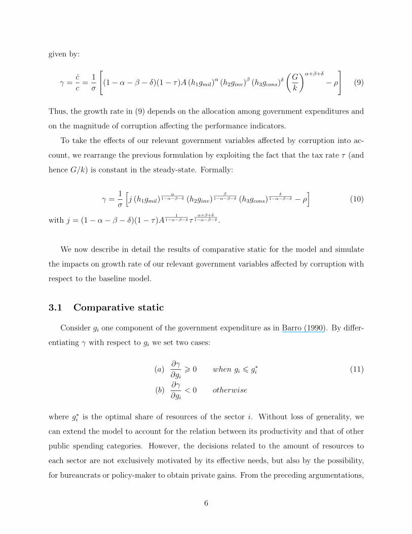
Thus, the growth rate in (9) depends on the allocation among government expenditures and

on the magnitude of corruption affecting the performance indicators.

To take the effects of our relevant government variables affected by corruption into ac-

count, we rearrange the previous formulation by exploiting the fact that the tax rate τ (and

hence G/k) is constant in the steady-state. Formally:

γ =1

σ

[j (h1gmil)

α1−α−β−δ (h2ginv)

β1−α−β−δ (h3gcons)

δ1−α−β−δ − ρ

](10)

with j = (1− α− β − δ)(1− τ)A1

1−α−β−δ τα+β+δ

1−α−β−δ .

We now describe in detail the results of comparative static for the model and simulate

the impacts on growth rate of our relevant government variables affected by corruption with

respect to the baseline model.

3.1 Comparative static

Consider gi one component of the government expenditure as in Barro (1990). By differ-

entiating γ with respect to gi we set two cases:

(a)∂γ

∂gi> 0 when gi 6 g∗i (11)

(b)∂γ

∂gi< 0 otherwise

where g∗i is the optimal share of resources of the sector i. Without loss of generality, we

can extend the model to account for the relation between its productivity and that of other

public spending categories. However, the decisions related to the amount of resources to

each sector are not exclusively motivated by its effective needs, but also by the possibility,

for bureaucrats or policy-maker to obtain private gains. From the preceding argumentations,

6

there are therefore some reasonable assumptions that can be included in our model in order

to derive a parametrization for empirical tests:

Assumption 1: the degree of exposure to corruption is not identical across categories of

government spending. As argued by Gupta et al. (2001) there are public sector like defence

that are more susceptible to corruptive practises.

Assumption 2: corruption has a negative impact on growth, i.e. ∂γ∂h< 0. That is, we

exclude that corruption might promote economic growth as it relaxes inefficient and rigid

regulations imposed by government (see for example, Dreher and Herzfeld (2005)).

Assumption 3: modelling corruption as a tax not only makes the impact of compo-

nents of government spending heterogenous on growth rates but focuses the channel of the

interactions (complementary or substitution) of corruption and government components by

the grand (or political) corruption (Bardhan, 1997). This restriction implies the exclusion

of inefficiency current government consumption on growth rate due to the effects of (petty)

corruption. With respect to the equation (8), this negligible impacts leads to h3∼= 1.

Assumption 4: the productivity of the expenditure of the public sectors is not homo-

geneous. In particular, this difference is modelled in the production function by assuming

that β (government investments) is greater than α (military sector).

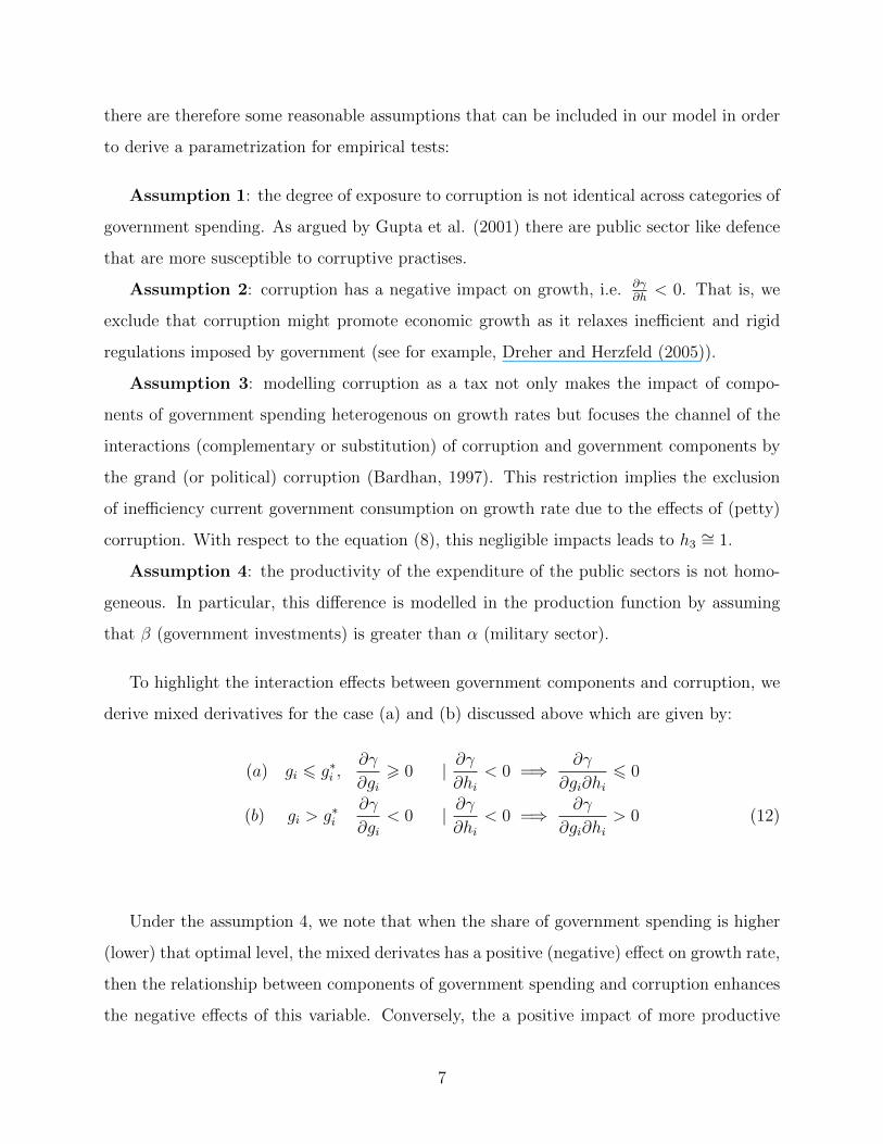
To highlight the interaction effects between government components and corruption, we

derive mixed derivatives for the case (a) and (b) discussed above which are given by:

(a) gi 6 g∗i ,∂γ

∂gi> 0 | ∂γ

∂hi< 0 =⇒ ∂γ

∂gi∂hi6 0

(b) gi > g∗i∂γ

∂gi< 0 | ∂γ

∂hi< 0 =⇒ ∂γ

∂gi∂hi> 0 (12)

Under the assumption 4, we note that when the share of government spending is higher

(lower) that optimal level, the mixed derivates has a positive (negative) effect on growth rate,

then the relationship between components of government spending and corruption enhances

the negative effects of this variable. Conversely, the a positive impact of more productive

7

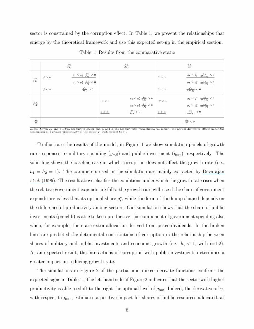
sector is constrained by the corruption effect. In Table 1, we present the relationships that

emerge by the theoretical framework and use this expected set-up in the empirical section.

Table 1: Results from the comparative static

dγdg1

dγdg2

dγdh

dγdg1

β > αg1 ≤ g∗1

dγdg1

≥ 0β > α

g1 ≤ g∗1dγ

dhdg1≤ 0

g1 > g∗1dγdg1

< 0 g1 > g∗1dγ

dhdg1> 0

β < α dγdg1

> 0 β < α dγdhdg1

< 0

dγdg2

β < αg2 ≤ g∗2

dγdg2

≥ 0β < α

g2 ≤ g∗2dγ

dhdg2≤ 0

g2 > g∗2dγdg2

< 0 g2 > g∗2dγ

dhdg2> 0

β > α dγdg2

> 0 β > α dγdhdg2

< 0

dγdh

dγdh

< 0

Notes: Given g1 and g2, two productive sector and α and β the productivity, respectively, we remark the partial derivative effects under theassumption of a greater productivity of the sector g2 with respect to g1.

To illustrate the results of the model, in Figure 1 we show simulation panels of growth

rate responses to military spending (gmil) and public investment (ginv), respectively. The

solid line shows the baseline case in which corruption does not affect the growth rate (i.e.,

h1 = h2 = 1). The parameters used in the simulation are mainly extracted by Devarajan

et al. (1996). The result above clarifies the conditions under which the growth rate rises when

the relative government expenditure falls: the growth rate will rise if the share of government

expenditure is less that its optimal share g∗i , while the form of the hump-shaped depends on

the difference of productivity among sectors. Our simulation shows that the share of public

investments (panel b) is able to keep productive this component of government spending also

when, for example, there are extra allocation derived from peace dividends. In the broken

lines are predicted the detrimental contributions of corruption in the relationship between

shares of military and public investments and economic growth (i.e., hi < 1, with i=1,2).

As an expected result, the interactions of corruption with public investments determines a

greater impact on reducing growth rate.

The simulations in Figure 2 of the partial and mixed derivate functions confirms the

expected signs in Table 1. The left hand side of Figure 2 indicates that the sector with higher

productivity is able to shift to the right the optimal level of ginv. Indeed, the derivative of γ,

with respect to ginv, estimates a positive impact for shares of public resources allocated, at

8

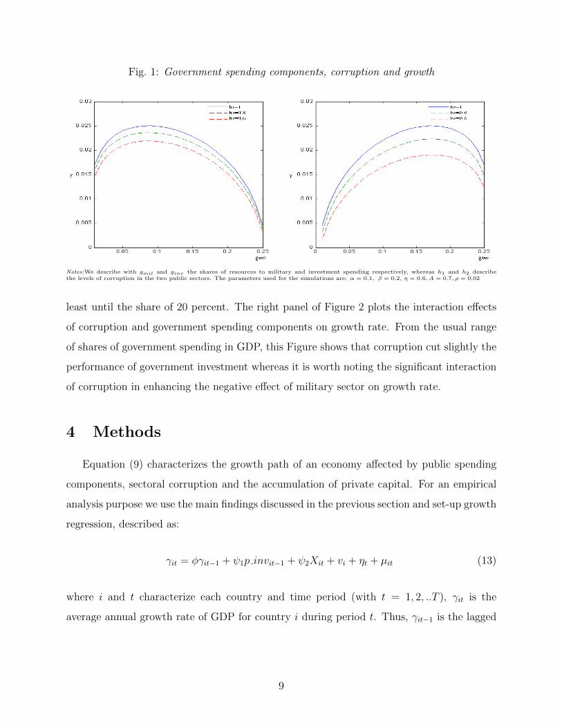
Fig. 1: Government spending components, corruption and growth

Notes:We describe with gmil and ginv the shares of resources to military and investment spending respectively, whereas h1 and h2 describethe levels of corruption in the two public sectors. The parameters used for the simulations are: α = 0.1, β = 0.2, η = 0.6, A = 0.7, ρ = 0.02

least until the share of 20 percent. The right panel of Figure 2 plots the interaction effects

of corruption and government spending components on growth rate. From the usual range

of shares of government spending in GDP, this Figure shows that corruption cut slightly the

performance of government investment whereas it is worth noting the significant interaction

of corruption in enhancing the negative effect of military sector on growth rate.

4 Methods

Equation (9) characterizes the growth path of an economy affected by public spending

components, sectoral corruption and the accumulation of private capital. For an empirical

analysis purpose we use the main findings discussed in the previous section and set-up growth

regression, described as:

γit = φγit−1 + ψ1p invit−1 + ψ2Xit + vi + ηt + µit (13)

where i and t characterize each country and time period (with t = 1, 2, ..T ), γit is the

average annual growth rate of GDP for country i during period t. Thus, γit−1 is the lagged

9

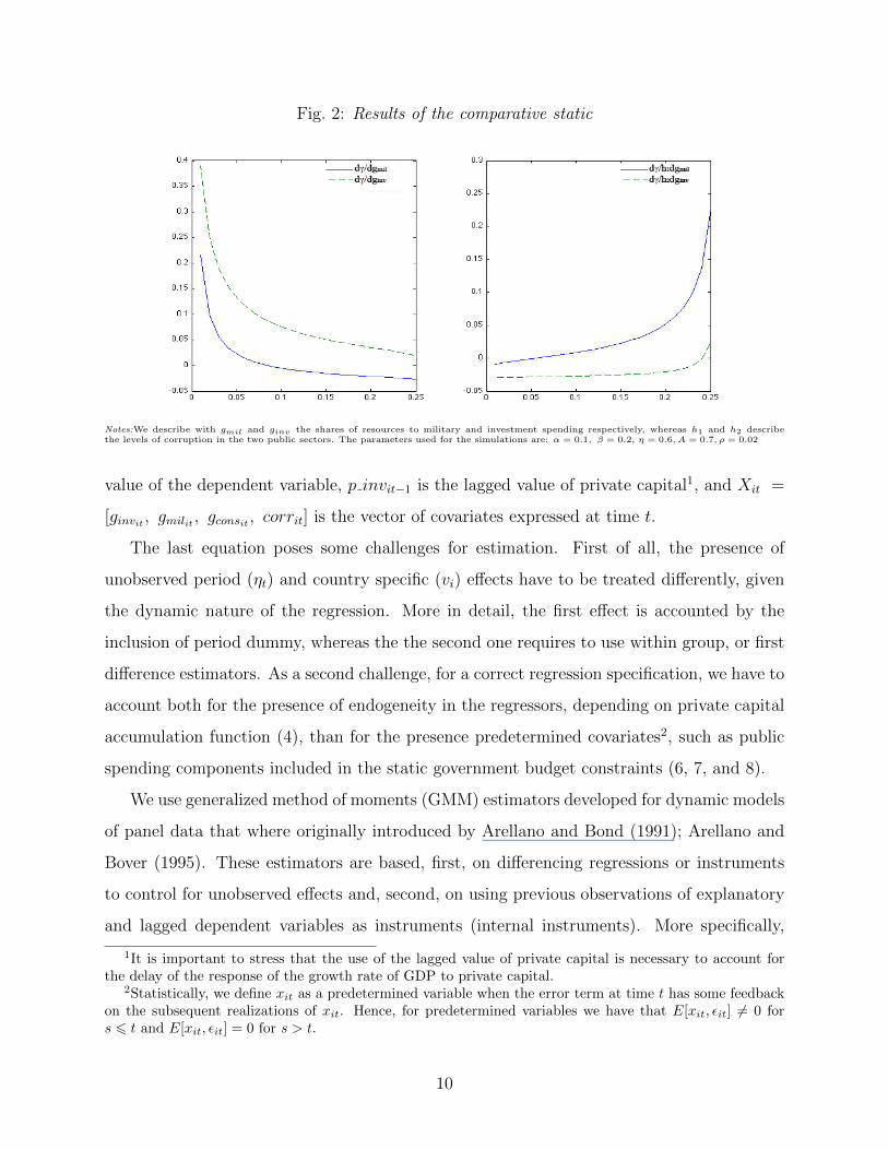
Fig. 2: Results of the comparative static

Notes:We describe with gmil and ginv the shares of resources to military and investment spending respectively, whereas h1 and h2 describethe levels of corruption in the two public sectors. The parameters used for the simulations are: α = 0.1, β = 0.2, η = 0.6, A = 0.7, ρ = 0.02

value of the dependent variable, p invit−1 is the lagged value of private capital1, and Xit =

[ginvit , gmilit , gconsit , corrit] is the vector of covariates expressed at time t.

The last equation poses some challenges for estimation. First of all, the presence of

unobserved period (ηt) and country specific (vi) effects have to be treated differently, given

the dynamic nature of the regression. More in detail, the first effect is accounted by the

inclusion of period dummy, whereas the the second one requires to use within group, or first

difference estimators. As a second challenge, for a correct regression specification, we have to

account both for the presence of endogeneity in the regressors, depending on private capital

accumulation function (4), than for the presence predetermined covariates2, such as public

spending components included in the static government budget constraints (6, 7, and 8).

We use generalized method of moments (GMM) estimators developed for dynamic models

of panel data that where originally introduced by Arellano and Bond (1991); Arellano and

Bover (1995). These estimators are based, first, on differencing regressions or instruments

to control for unobserved effects and, second, on using previous observations of explanatory

and lagged dependent variables as instruments (internal instruments). More specifically,

1It is important to stress that the use of the lagged value of private capital is necessary to account forthe delay of the response of the growth rate of GDP to private capital.

2Statistically, we define xit as a predetermined variable when the error term at time t has some feedbackon the subsequent realizations of xit. Hence, for predetermined variables we have that E[xit, εit] 6= 0 fors 6 t and E[xit, εit] = 0 for s > t.

10

following Arellano and Bond (1991); Arellano and Bover (1995), we can rewrite equation

(13) as:

∆γit = φ∆γit−1 + ψ1∆p invit−1 + ψ2∆Xit + ∆µit (14)

where all variables are now expressed as deviations from period mean and t = 3, .., T . Equa-

tion (14) violate the assumption of non correlation between the error term µit − µit−1, and

the lagged dependent variable γit − γit−1. Thus, the use of instruments is required in order

to deal, contemporary, with the likely endogeneity between errors and lagged values of the

dependent variable and with the endogenity in the regressors. The instruments take advan-

tage of the panel nature of the dataset in that they consist of previous observations of the

explanatory and lagged-dependent variables.

Under the assumption of non serial correlation in the the error term and that the explana-

tory variables are weakly exogenous3, our application of the GMM dynamic panel estimator

uses the following moment conditions:

E [γit−2 (µit − µit−1)] = 0 (15)

E[Xit−2 (µit − µit−1)

]= 0 (16)

where X now include in it both the exogenous covariates and private capital p inv. In theory

un unlimited number of moment conditions, which implies the use of a number of instruments

growing with the number of periods T, may increase the efficiency of the estimator, at the

expense of an increasing of the overfitting bias. The trade-off between efficiency and bias

in the estimator becomes not trivial especially when the sample size in the cross-sectional

dimension is limited (Roodman, 2009). Since this is our case, we use as instruments only

the first appropriate lag of each time-varying explanatory variable.

The GMM estimator based on conditions (15) and (16), is known as difference estimator.

Notwithstanding its advantages with respect to simpler panel-data estimators, the differ-

ence estimator has important statistical shortcomings. As point out by Blundell and Bond

(1998) among others, when the explanatory variables are persistent over time, lagged levels

3By definition a variable is weakly exogenous when it is assumed to be uncorrelated with future realizationsof the error terms.

11

of these variables are weak instruments in the first difference specification of the growth re-

gression. Note that, the weakness of instruments influences the asymptotic and small-sample

performance of the difference estimator toward inefficient and biased coefficient estimates,

respectively.

To prevent the potential inefficiency and bias in the difference estimator, we adopt a

strategy which combine the specification in difference (14), with the regression equation in

levels (13) into an unique system of equations (Arellano and Bover, 1995; Blundell and Bond,

1998). Moreover, we use the set of instruments described above for the regression equation

in difference, and the lagged differences of the explanatory variables for the equation in

levels. These are appropriate instruments under the assumption that the correlation between

explanatory variables and the country-specific effect (vi) is the same for all time periods.

That is:

E [γit+pvi] = E [Zit+qvi] and (17)

E[Xit+pvi

]= E [Xit+qvi] for all p and q (18)

Using the stationarity property and the assumption of exogeneity of future shocks, the

moment conditions for the second part of the system are given by:

E [(γit−1 − Zit−2) (µit + vi)] = 0 (19)

E[(Xit−1 −Xit−2

)(µit + vi)

]= 0 (20)

Thus, we use moment conditions (15), (16), (19), and (20) and employ a GMM procedure to

generate consistent and efficient estimates of the parameters of interest and their asymptotic

variance and covariance matrix, which are described respectively by the following formulas:

θ =(X ′ZΩZ ′X

)−1

X ′ZΩZ ′y (21)

AV AR(θ) =(X ′ZΩZ ′X

)−1

(22)

where θ = [φ, ψi] is the vector of parameters, y is the dependent variable stacked first in

12

differences and then in levels, x is the matrix of covariates which includes also the lagged

values of the dependent variable and the private investment stacked first in differences and

then in levels, Z is the matrix of instruments, and Ω is a consistent estimate of the variance-

covariance matrix of the moment conditions. Estimations of the variance-covariance matrix

are obtained through two-step procedure (Arellano and Bond, 1991). This procedure consist

in: i) assuming that the residual µit are independent and homoskedastic both across countries

and over time, to obtain the first step parameter estimations, and ii) using the residual in

the first step estimations to obtain a consistent variance-covariance matrix, and then to

re-estimate the parameters of the model in the second-step.

Since the consistency of the GMM estimators depends on whether lagged values of the

explanatory variables are valid instruments in the growth regression, we set-up different

tests for it. Firstly, we examine the overidentifying restrictions and test the validity of the

instruments by analyzing the sample similar to the moment conditions used in the estimation

process. In particular, Hansen and incremental Hansen tests examine the validity of the full

set of instruments and the instruments included in the level equation, respectively. Failure to

reject the inability of the instrument set gives support to the model specification. Further, a

test for serially correlated errors is implemented. With this dynamic framework, the absence

of a second-order residual correlation is tested for the validity of the estimation under the

null hypothesis.

Finally for a policy-maker perspective, using the estimated parameters from the system

GMM model, we propose different elasticity measures. The objective is threefold: i) to

analyse the direct elasticity of military spending, public investments and corruption on the

growth rate of GDP; ii) to assess the interactions among public spending components and

corruption, by calculating an indirect elasticity measure, and iii) to derive the share of these

elasticities on total elasticities.

Following the suggestion proposed by Lee (2006) we define the direct elasticity as:

ed = πX ′(.,.) (23)

where ˜X(.,.) = [gmil/γ, ginv/γ, corr/γ] is a vector of ratios among military spending, public

13

investments and corruption constructed as country and period means and the growth rate of

GDP constructed as country and period mean, whereas π = [ψgmil, ψginv , ψcorr] is a vector

of parameters estimated by equation (21). For example the direct elasticity of military

spending is then given by:

miled = ψgmilgmil(.,.)γ(.,.)

(24)

Moreover, to estimate indirect elasticity we set-up a fixed effect panel data estimator, which

regress, one by one, the component of X on the other components, and a linear deterministic

trend (T) to control for cyclical effects. For example, the specification of the fixed effect panel

data for military spending is given by:

milit = a+ b1ginvit + b2corrit + T + ui +mit (25)

where ui is the country specific effect, and mit is the error term. The parameters estimated

by (24) and (25), are then used to obtain the indirect elasticity for military spending with

respect corruption, described as:

mil/g correind = (ψcorrb2)gmil(.,.)γ(.,.)

(26)

Finally, total elasticity measure is obtained as the sum of direct and indirect elasticities for

each component. In our example, the total elasticity of military spending is then given by:

miletot =mil ed +mil/corr eind +mil/g inv eind (27)

5 Empirical results

5.1 Data

The dataset used to estimate the system of equations (13) and (14) includes 22 African

countries over the period 1996-2007 and it is extracted from African development indicator

of the World Bank (WBI). The complete list of countries is reported in Appendix 1, along

with the mean of each used variable.

14

Dependent variable (γ) is represented by the percentage annual growth rate of GDP

per-capita, whereas (ginv) is matched by the percentage ratio of gross private investment in

GDP, which includes private nonprofit agencies in addiction to the fixed domestic assets.

Government spending components are characterized by three different variables: i) mil-

itary expenditures which includes all current and capital expenditures on the armed forces

from NATO definition. It includes peacekeeping forces not only defense ministries and other

government agencies engaged in defense projects but also paramilitary forces, if these are

judged to be trained and equipped for military operations and military space activities;

ii)gross domestic fixed investment (i.e., gross fixed capital formation) comprises all additions

to the stocks of fixed assets (purchases and own-account capital formation), less any sales of

second-hand and scrapped fixed assets, by government units and non-financial public enter-

prises. It is worth noting that the variable outlays by government on military equipment are

excluded; iii) government consumption, which includes current expenditures for purchases of

goods and services (including compensation of employees). These components of government

spending are expressed as percentage in GDP.

A measure of corruption is included in the model to account for direct and indirect in-

teractions with growth rate. Although different private or public agencies publish measures

of corruption for countries of the World, we use the control of corruption index (CCI) ex-

tracted from WBI which is based on direct perceptions of firms. This index is interpreted

as the extent to which public power is exercised for private gain, including administrative

and grand corruption, as well as capture of the state by elites and private interests. Because

we are not able to drop-out from the variable the influence of other forms of corruption, we

expect a certain degree of measurement error (in excess with respect to grand corruption

that we specify in the model) in using this variable. The corruption index proposed ranges

from 0 to 100, where 0 means that country is perceived corrupted.

In addition to this set of variables, we define a dummy characterizing the countries in

the sub-Saharan africa (equal to 1), d.sub saharian, and 0 otherwise.

15

5.2 Estimates

Table 2 shows Blundell and Bond (1998) GMM estimation results for system of equations

13 and 14. The first two columns of the table are used as benchmark, including public

spending components and private investments (I) and time dummies (II), respectively;

column (III) introduces corruption index whereas column (IV ) includes the interaction

terms for military sector (gmilt ∗ corrt) and public investments (ginvt ∗ corrt). The lagged

value of private investment is introduced to account for its accumulation function described

in equation 4.

The estimated coefficients are significant, except for the interaction term of public in-

vestments (ginvt ∗ corrt ), and exhibit the expected signs. This outcome confirms the good

ability of the proposed endogenous growth model to explain the nexus among public spend-

ing components, corruption and growth. More in details, from column III, we see that the

share of military spending in GDP exhibits a strong negative impact on the growth rate of

GDP whereas, conversely, public investments are positive relate to it. This result predict

a different productivity level of the two components of public spending, and suggests that

the amount of resources devoted by the government to the military sector exceed its optimal

needs. In this context, corruption does not only entail a decrease in economic performance,

but it also increase the amount of rent-seeking activities, i.e. military spending. As a first

assessment, the theoretical prediction clearly emerges from the estimation (IV ) where the

interaction variable gmilt ∗ corrt affects positively the response variable. On the contrary,

the statistically not significant interaction of ginvt ∗ corrt excludes important effects in the

relationship between the public investment sector and growth rate.

Such a conclusion, corruption, in the African context, is able to favour military spend-

ing, worsening the negative impact of larger military sector on the economy’s growth rate.

Corruption entails the presence of re-allocative effects, which are independent by the pro-

ductivity or efficiency of the sector, but are related to them abilities to generates more rents,

involving bigger amount of money, and so larger bribes (Delavallade, 2005).

Table 3 reports the fixed-effect panel estimation results for the auxiliary regression 25,

useful to measure by (26) the indirect elasticities of military spending, public investments,

16

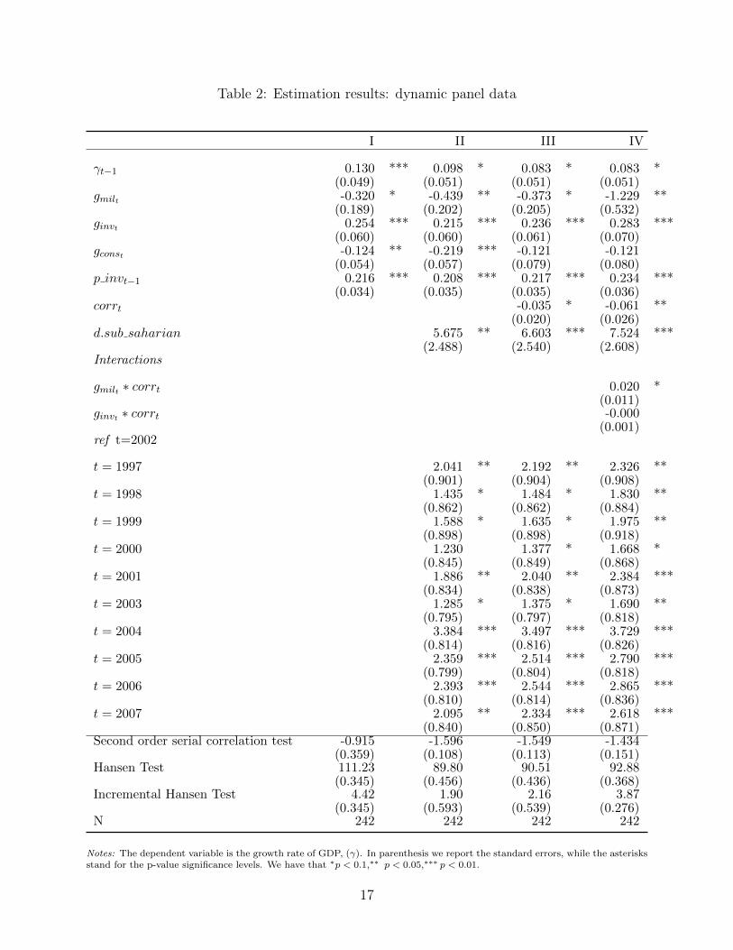
Table 2: Estimation results: dynamic panel data

I II III IV

γt−1 0.130 *** 0.098 * 0.083 * 0.083 *(0.049) (0.051) (0.051) (0.051)

gmilt -0.320 * -0.439 ** -0.373 * -1.229 **(0.189) (0.202) (0.205) (0.532)

ginvt 0.254 *** 0.215 *** 0.236 *** 0.283 ***(0.060) (0.060) (0.061) (0.070)

gconst -0.124 ** -0.219 *** -0.121 -0.121(0.054) (0.057) (0.079) (0.080)

p invt−1 0.216 *** 0.208 *** 0.217 *** 0.234 ***(0.034) (0.035) (0.035) (0.036)

corrt -0.035 * -0.061 **(0.020) (0.026)

d.sub saharian 5.675 ** 6.603 *** 7.524 ***(2.488) (2.540) (2.608)

Interactions

gmilt ∗ corrt 0.020 *(0.011)

ginvt ∗ corrt -0.000(0.001)

ref t=2002

t = 1997 2.041 ** 2.192 ** 2.326 **(0.901) (0.904) (0.908)

t = 1998 1.435 * 1.484 * 1.830 **(0.862) (0.862) (0.884)

t = 1999 1.588 * 1.635 * 1.975 **(0.898) (0.898) (0.918)

t = 2000 1.230 1.377 * 1.668 *(0.845) (0.849) (0.868)

t = 2001 1.886 ** 2.040 ** 2.384 ***(0.834) (0.838) (0.873)

t = 2003 1.285 * 1.375 * 1.690 **(0.795) (0.797) (0.818)

t = 2004 3.384 *** 3.497 *** 3.729 ***(0.814) (0.816) (0.826)

t = 2005 2.359 *** 2.514 *** 2.790 ***(0.799) (0.804) (0.818)

t = 2006 2.393 *** 2.544 *** 2.865 ***(0.810) (0.814) (0.836)

t = 2007 2.095 ** 2.334 *** 2.618 ***(0.840) (0.850) (0.871)

Second order serial correlation test -0.915 -1.596 -1.549 -1.434(0.359) (0.108) (0.113) (0.151)

Hansen Test 111.23 89.80 90.51 92.88(0.345) (0.456) (0.436) (0.368)

Incremental Hansen Test 4.42 1.90 2.16 3.87(0.345) (0.593) (0.539) (0.276)

N 242 242 242 242

Notes: The dependent variable is the growth rate of GDP, (γ). In parenthesis we report the standard errors, while the asterisksstand for the p-value significance levels. We have that ∗p < 0.1,∗∗ p < 0.05,∗∗∗ p < 0.01.

17

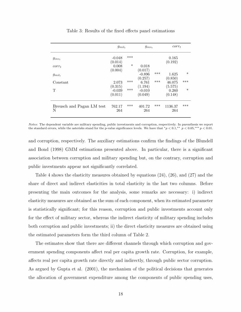
Table 3: Results of the fixed effects panel estimations

gmilt ginvt corrt

ginvt -0.048 *** 0.165(0.014) (0.192)

corrt 0.008 * 0.018(0.004) (0.017)

gmilt -0.896 *** 1.625 *(0.257) (0.850)

Constant 2.073 *** 6.761 *** 46.075 ***(0.315) (1.194) (5.575)

T -0.039 *** -0.010 0.260 *(0.011) (0.049) (0.148)

Breusch and Pagan LM test 762.17 *** 401.72 *** 1136.37 ***N 264 264 264

Notes: The dependent variable are military spending, public investments and corruption, respectively. In parenthesis we reportthe standard errors, while the asterisks stand for the p-value significance levels. We have that ∗p < 0.1,∗∗ p < 0.05,∗∗∗ p < 0.01.

and corruption, respectively. The auxiliary estimations confirm the findings of the Blundell

and Bond (1998) GMM estimations presented above. In particular, there is a significant

association between corruption and military spending but, on the contrary, corruption and

public investments appear not significantly correlated.

Table 4 shows the elasticity measures obtained by equations (24), (26), and (27) and the

share of direct and indirect elasticities in total elasticity in the last two columns. Before

presenting the main outcomes for the analysis, some remarks are necessary: i) indirect

elasticity measures are obtained as the sum of each component, when its estimated parameter

is statistically significant; for this reason, corruption and public investments account only

for the effect of military sector, whereas the indirect elasticity of military spending includes

both corruption and public investments; ii) the direct elasticity measures are obtained using

the estimated parameters form the third column of Table 2.

The estimates show that there are different channels through which corruption and gov-

ernment spending components affect real per capita growth rate. Corruption, for example,

affects real per capita growth rate directly and indirectly, through public sector corruption.

As argued by Gupta et al. (2001), the mechanism of the political decisions that generates

the allocation of government expenditure among the components of public spending uses,

18

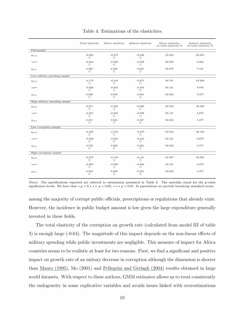
Table 4: Estimations of the elasticities

Total elasticity Direct elasticity Indirect elasticity Direct elasticity Indirect elasticityon total elasticity % on total elasticity %

Full-sample

gmil -0.820 -0.273 -0.546 33.345 66.655() () ()

corr -0.644 -0.585 -0.058 90.936 9.064() () ()

ginv 0.560 0.520 0.040 92.879 7.121() () ()

Low military spending sample

gmil -0.175 -0.104 -0.071 40.701 59.299() () ()

corr -0.626 -0.043 -0.583 93.121 6.879() () ()

ginv 0.628 0.034 0.594 94.623 5.377() () ()

High military spending sample

gmil -0.611 -0.223 -0.389 63.552 36.448() () ()

corr -0.631 -0.043 -0.588 93.121 6.879() () ()

ginv 0.451 0.024 0.427 94.623 5.377() () ()

Low corruption sample

gmil -0.425 -0.155 -0.270 63.552 36.448() () ()

corr -0.366 -0.025 -0.341 93.121 6.879() () ()

ginv 0.533 0.029 0.504 94.623 5.377() () ()

High corruption sample

gmil -0.279 -0.158 -0.121 43.307 56.693() () ()

corr -0.865 -0.060 -0.806 93.121 6.879() () ()

ginv 0.564 0.030 0.534 94.623 5.377() () ()

Notes: The specifications reported are referred to estimations presented in Table 2. The asterisks stand for the p-valuesignificance levels. We have that ∗ p < 0.1, ∗ ∗ p < 0.05, ∗ ∗ ∗ p < 0.01. In parentheses we provide bootstrap standard errors.

among the majority of corrupt public officials, prescriptions or regulations that already exist.

However, the incidence in public budget amount is low given the large expenditure generally

invested in these fields.

The total elasticity of the corruption on growth rate (calculated from model III of table

3) is enough large (-0.64). The magnitude of this impact depends on the non-linear effects of

military spending while public investments are negligible. This measure of impact for Africa

countries seems to be realistic at least for two reasons. First, we find a significant and positive

impact on growth rate of an unitary decrease in corruption although the dimension is shorter

than Mauro (1995), Mo (2001) and Pellegrini and Gerlagh (2004) results obtained in large

world datasets. With respect to these authors, GMM estimator allows us to treat consistently

the endogeneity in some explicative variables and avoids issues linked with overestimations

19

of OLS parameters. Secondly, the existence on average of weaker institutions in Africa makes

corruption work as the second-best solution to market distortions imposed by government

procedures and policies at least in the short run. This effect partly counterbalance the

negative impact of corruption on economic performance in the long run.

We find a larger growth rate impact of changes in military spending. Also in this case,

a 10% decrease in military allocation may enhance real per capita growth rate by 8.2% on

growth rate. It is confirmed that rent-seeking sectors as military more than other productive

sectors is dependent from corruptive practices. Indirect elasticity seems to be associated

with the levels of corruption as shown in the sub-sample estimations of the elasticities.

This can support a political intervention to enhance the economic performance that

directly leads to a cut in the share of military spending to GDP, and indirectly reduces

corruptive incentives yielded by the defence sector. From a policy-maker point of view, if

the resources depicted by the military sector are devoted to enhance the share of public

investment, the impact in terms of real per capita growth rate, conditionally to corruption

level, rise. In table 4 we also present the estimated elasticities of sub-samples of countries

selected by distribution of the variable military spending in GDP; the sample ”‘high”’ repre-

sents the countries over the median of the distribution whereas ”‘low”’ represents the group

under the median. The estimated values of corruption in these sub-samples are shown to

be close estimates of those reported for the full sample of African countries, whereas are

growing in countries where the military spending is significantly more higher. The result of

this sensitivity analysis proves the usefulness to disentangle the effect of complementarities

between military sector and corruption as well as the goodness of our previous conclusions.

20

6 Conclusions

Corruption in developing countries is largely accepted to be an important obstacle to

economic growth, but there has been relatively few attempt to identify the specific manner

in which this may occur. In this paper an endogenous growth model that allows corruption

to act on economic growth, through interactions between the military sector and civilian

investments is developed and estimated. The empirical results for a panel of African coun-

tries confirm the predictions that while government investments enhance economic growth,

large military burdens and current government spending reduce it and that corruption has

a negative effect. Significant indirect effects of corruption are found for each components

of government spending, with a particularly strong asymmetric effect for the military com-

ponent. This negative effect of military burden on growth is consistently influenced by

the indirect impact of corruption, while the reverse effect though significant is considerably

smaller. This implies that combatting corruption is likely to directly increase aggregate

economic performances and to indirectly cut the negative impacts of military spending.

Overall, the results provide strong evidence that for the group of African countries studies

high levels of defense spending and corruption have had a damaging effect on economic

performance, both directly and indirectly.

21

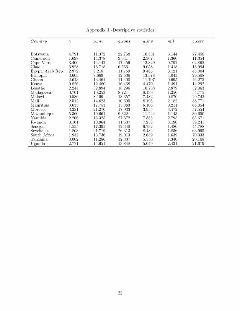
Appendix 1 -Descriptive statistics

Country γ p inv g cons g inv mil g corr

Botswana 4.791 11.372 22.768 10.531 3.144 77.458Cameroon 1.698 14.378 9.641 2.367 1.360 11.354Cape Verde 3.406 14.142 17.456 12.329 0.792 62.862Chad 3.928 16.718 6.566 9.058 1.418 13.994Egypt, Arab Rep. 2.972 9.218 11.769 9.485 3.121 45.004Ethiopia 3.603 8.669 12.536 13.378 4.043 29.508Ghana 2.613 13.461 11.400 11.707 0.695 46.275Kenya 0.826 12.480 16.468 4.470 1.491 14.292Lesotho 2.244 32.894 18.296 10.738 2.879 52.063Madagascar 0.701 10.253 8.721 8.139 1.250 54.775Malawi 0.586 8.199 13.357 7.482 0.870 29.742Mali 2.512 14.623 10.695 8.195 2.182 38.771Mauritius 3.633 17.753 13.383 6.106 0.211 68.054Morocco 3.231 21.270 17.933 3.955 3.472 57.554Mozambique 5.360 10.661 9.322 11.244 1.143 30.650Namibia 2.266 16.325 27.372 7.885 2.795 65.671Rwanda 3.101 10.964 11.537 7.258 3.190 39.241Senegal 1.555 17.395 12.340 6.732 1.480 45.788Seychelles 1.808 21.719 26.313 8.482 1.856 63.995South Africa 1.932 13.736 19.013 2.689 1.639 70.333Tanzania 3.002 11.286 12.337 5.550 1.340 20.108Uganda 2.771 14.651 13.848 5.049 2.431 21.679

22

References

Acemoglu, D. and Verdier, T. (1998). Property rights, corruption and the allocation of

talent: A general equilibrium approach. Economic Journal, 108 (450), 1381–1403.

Aizenman, J. and Glick, R. (2003). Military Expenditure, Threats, and Growth. NBER

Working Papers 9618, National Bureau of Economic Research, Inc.

Arellano, M. and Bond, S. (1991). Some tests of specification for panel data: Monte

carlo evidence and an application to employment equations. Review of Economic Studies,

58 (2), 277–97.

— and Bover, O. (1995). Another look at the instrumental variable estimation of error-

components models. Journal of Econometrics, 68 (1), 29–51.

Barro, R. J. (1990). Government spending in a simple model of endogenous growth. Jour-

nal of Political Economy, 98 (5), S103–26.

Blundell, R. and Bond, S. (1998). Initial conditions and moment restrictions in dynamic

panel data models. Journal of Econometrics, 87 (1), 115–143.

Delavallade, C. (2005). Corruption and distribution of public spending in developing

countries. Journal of Economics and Finance, 30 (2).

— (2007). Why do North African firms involve in corruption ? Documents de travail du

Centre d’Economie de la Sorbonne v07002, Universite Pantheon-Sorbonne (Paris 1), Cen-

tre d’Economie de la Sorbonne.

Devarajan, S., Swaroop, V. and Heng-fu, Z. (1996). The composition of public ex-

penditure and economic growth. Journal of Monetary Economics, 37 (2-3), 313–344.

Dreher, A. and Herzfeld, T. (2005). The Economic Costs of Corruption: A Survey and

New Evidence. Public Economics 0506001, EconWPA.

Gupta, S., Sharan, R. and de Mello, L. (2000). Corruption and Military Spending.

IMF Working Papers 00/23, International Monetary Fund.

23

Lee, J.-H. (2006). Business corruption, public sector corruption, and growth rate: time

series analysis using korean data. Applied Economics Letters, 13 (13), 881–885.

Mariani, F. (2007). Migration as an antidote to rent-seeking? Journal of Development

Economics, 84 (2), 609–630.

Mauro, P. (1995). Corruption and growth. The Quarterly Journal of Economics, 110 (3),

681–712.

— (1998). Corruption and the composition of government expenditure. Journal of Public

Economics, 69 (2), 263–279.

Pellegrini, L. and Gerlagh, R. (2004). Corruption’s effect on growth and its transmis-

sion channels. Kyklos, 57 (3), 429–456.

Roodman, D. (2009). A note on the theme of too many instruments. Oxford Bulletin of

Economics and Statistics, 71 (1), 135–158.

Tanzi, V. (1998). Corruption Around the World - Causes, Consequences, Scope, and Cures.

IMF Working Papers 98/63, International Monetary Fund.

24