arX

iv:1

202.

6491

v1 [

astr

o-ph

.CO

] 2

9 Fe

b 20

12Draft version March 1, 2012Preprint typeset using LATEX style emulateapj v. 5/2/11

COSMOS: STOCHASTIC BIAS FROM MEASUREMENTS OF WEAK LENSING AND GALAXY CLUSTERING

Eric Jullo1,2, Jason Rhodes1, Alina Kiessling3, James E. Taylor4, Richard Massey3, Joel Berge5, CarloSchimd2, Jean-Paul Kneib2, and Nick Scoville6

Draft version March 1, 2012

ABSTRACT

In the theory of structure formation, galaxies are biased tracers of the underlying matter densityfield. The statistical relation between galaxy and matter density field is commonly referred as galaxybias. In this paper, we test the linear bias model with weak-lensing and galaxy clustering measurementsin the 2 square degrees COSMOS field (Scoville et al. 2007). We estimate the bias of galaxies betweenredshifts z = 0.2 and z = 1, and over correlation scales betweenR = 0.2 h−1 Mpc and R = 15 h−1 Mpc.We focus on three galaxy samples, selected in flux (simultaneous cuts I814W < 26.5 and Ks < 24),and in stellar-mass (109 < M∗ < 1010 h−2 M⊙ and 1010 < M∗ < 1011 h−2 M⊙). At scales R >2 h−1Mpc, our measurements support a model of bias increasing with redshift. The Tinker et al.(2010) fitting function provides a good fit to the data. We find the best fit mass of the galaxy halosto be log(M200/h

−1M⊙) = 11.7+0.6−1.3 and log(M200/h

−1M⊙) = 12.4+0.2−2.9 respectively for the low and

high stellar-mass samples. In the halo model framework, bias is scale-dependent with a change ofslope at the transition scale between the one and the two halo terms. We detect a scale-dependenceof bias with a turn-down at scale R = 2.3± 1.5h−1Mpc, in agreement with previous galaxy clusteringstudies. We find no significant amount of stochasticity, suggesting that a linear bias model is sufficientto describe our data. We use N-body simulations to quantify both the amount of cosmic variance andsystematic errors in the measurement.Subject headings: cosmology: observations — gravitational lensing: weak — large-scale structure of

Universe

1. INTRODUCTION

In the theory of structure formation, galaxies form indark matter overdensities. However, the distribution ofgalaxies does not perfectly match the underlying matterdistribution, and the relation between the two is calledgalaxy bias.The galaxy bias relation δg = f(δ) relates the mat-

ter density contrast δ to the galaxy density contrast δg.The density contrast δ is defined as the ratio betweenthe local and the mean densities δ ≡ ρ/ρ − 1. To firstorder, the galaxy bias relation δg = bδ is parametrizedby the bias parameter b. However the stochasticity inthe physical processes of galaxy formation might intro-duce some stochasticity in the galaxy bias relation. Theamount of stochasticity can be measured with the cor-relation coefficient r defined as the ratio between thecovariance and the variance of the density contrasts δ

and δg, r = 〈δgδ〉/√

〈δ2g〉〈δ2〉. A correlation coefficient

r = 1 means the bias relation is perfectly linear, whereas0 < r < 1 suggests stochasticity and/or non-linearity

eric.jullo@oamp.fr1 Propulsion Laboratory, California Institute of Technology,

Pasadena, CA 91109, USA2 Laboratoire dAstrophysique de Marseille, Universite de

Provence, CNRS, 13388 Marseille CEDEX 13, France3 Institute for Astronomy, Blackford Hill, Edinburgh EH9 3HJ

UK4 Department of Physics and Astronomy, University of Wa-

terloo, 200 University Avenue West, Waterloo, Ontario, CanadaN2L

5 Institute of Astronomy, Department of Physics, ETH Zurich,CH-8093, Switzerland

6 California Institute of Technology, MC 105-24, 1200 EastCalifornia Boulevard, Pasadena, CA 91125, USA

(Dekel & Lahav 1999). We do not expect the bias re-lation to be anti-correlated with r < 0, nor b < 0 (i.e.galaxy clustering decreases when matter clustering in-creases).Bias varies for different galaxy populations. Galaxy bi-

asing is known to be larger for luminous, red, and high-redshift galaxies (Marinoni et al. 2005; Meneux et al.2006; Coil et al. 2008; Zehavi et al. 2010). Bias alsovaries with scale, but differently for different galaxy typesand luminosity (Cresswell & Percival 2009; Ouchi et al.2005; McCracken et al. 2010). In the halo-model frame-work, the scale-dependence of bias is explained as thetransition from a small-scale regime where galaxiesare in the same halo of dark matter to a large-scaleregime where galaxies are in two different halos (see e.g.Zheng et al. 2009, for a recent discussion). The scale-dependence of bias therefore tells us about the dark mat-ter halo properties around galaxies.Tegmark & Bromley (1999) first measured bias

stochasticity in the Las Campanas Redshift Survey. Atthe same time, simulations started to predict stochastic-ity, as well as scale and redshift-dependence in the biasrelation due to physical processes (Blanton et al. 1999;Somerville et al. 2001; Yoshikawa et al. 2001). In the2dF Galaxy Redshift Survey, Wild et al. (2005) usedthe count-in-cell technique to measure the non-linearityand stochasticity of the bias relation for red/earlyand blue/late-type galaxies at redshift z < 0.114. Forboth categories, they found more stochasticity at scaleR = 10 Mpc than at scale R = 45 Mpc. Recent resultsfrom simulations also predict an increasing amount ofstochasticity at smaller scales (Baldauf et al. 2010).The correlation coefficient is at the same time an esti-

2

mate of stochasticity and non-linearity. In the zCOS-MOS redshift survey (Lilly et al. 2009), Kovac et al.(2009) found non-linearity to contribute less than ∼0.2% to the bias relation for luminosity-selected galax-ies (MB < −20− z). Therefore in the following, we willassume that the correlation coefficient r mostly quanti-fies bias stochasticity. With respect to the bias param-eter b, Kovac et al. (2009) found the bias relation to bescale-independent between scales R = 8 h−1 Mpc andR = 10 h−1 Mpc, and redshift-dependent between red-shifts z = 0.4 and z = 1.In this work, we measure galaxy bias with a technique

proposed by Schneider (1998) based on galaxy cluster-ing and weak lensing. In short, weak lensing is used toderive matter clustering from the shape of backgroundgalaxies, which is then compared to the galaxy cluster-ing to infer the bias. van Waerbeke et al. (1999) em-phasized the potential of this technique with analyti-cal calculations for surveys with various depths and ar-eas, and Hoekstra et al. (2001, 2002) applied it to the50.5 deg2 of the RCS and VIRMOS-DESCART sur-veys. They measured the linear bias parameter b andthe correlation coefficient r for a flux-limited galaxy sam-ple (19.5 < RC < 21) at redshift z ≃ 0.35, and onscales between R = 0.2 and 9.3 h−1

50 Mpc. They foundstrong evidence that both b and r change with scale, andr ∼ 0.57 at 1 h−1

50 Mpc, which suggests a significant de-gree of stochasticity and/or non-linearity in their sampleof galaxies. Simon et al. (2007) applied the same tech-nique to the 15 deg2 of the GaBoDS survey for threeflux-limited galaxy samples in the R-band, at redshiftz =0.35, 0.47 and 0.61. They also found bias to be scaledependent, with an increasing amount of bias at smallscales. In addition, they found the bias parameters band r to be redshift-independent within statistical uncer-tainties, with r ∼ 0.6. Finally, Sheldon et al. (2004) per-formed a comparable study in the 3800 deg2 of the SDSSsurvey, with volume- and magnitude-selected galaxies(0.1 < z < 0.174 and −23.0 < Mr − 5 logh < −21.5). Inagreement with Hoekstra et al. (2002), they found theratio b/r to be scale-independent between 0.4 and 6.7h−1 Mpc, with (b/r) = (1.3 ± 0.2)(Ωm/0.27) for a flux-limited galaxy sample. In fact, the Hoekstra et al. (2002)results suggested that the respective scale-dependence ofb and r conspire to produce a scale-independent ratiob/r. In summary, the consistent value of r < 1 found inall these studies suggests some degree of stochasticity inthe investigated galaxy samples.In this work, we study the bias of galaxies in the 2

square degrees of the COSMOS field. We test the lin-ear bias model, and its dependence on scale and redshift.For two galaxy samples selected in stellar mass and onesample selected in flux, we measure bias on scales be-tween 0.2 h−1 Mpc and 15 h−1 Mpc, and redshifts be-tween z = 0.2 and z = 1. Thus, we extend the pre-vious works on bias both in scale, redshift and stellarmass. COSMOS is ideal to perform this study becauseaccurate stellar mass have been measured up to redshiftz ∼ 1.2 (Bundy et al. 2010), and photometric redshiftsup to redshift z ∼ 4 (Ilbert et al. 2009). In addition,with the high resolution images from the the AdvancedCamera for Survey aboard the Hubble Space Telescope(ACS/HST), we can precisely measure the shape of more

than 200,000 galaxies. Measuring the shape of galaxiesat redshift z > 2 is crucial for weak lensing to allow ac-curate determination of the matter density up to redshiftz ∼ 1. In section 2, we present the COSMOS survey, ourlensing catalog and our selection of foreground galaxiesfor which we want to measure the bias. In section 3, wedescribe the lensing formalism used in this paper. In sec-tion 4, we present a set of simulations we use to quantifythe impact of cosmic variance. In section 5, we show ourresults, and we go on to discuss some possible systematicerrors in section 6. We conclude in section 7.In this paper, we assume the WMAP7 (Komatsu et al.

2010) cosmological parameters Ωm = 0.272, ΩΛ = 0.728,Ωb = 0.0449, σ8 = 0.809, n = 0.963, ω0 = −1 andh = 0.71.

2. DATA

2.1. General properties

The COSMOS field is a 1.64 deg2 patch of sky closeto the equator (α=10.h00.m28.s, δ=+2.12.′21.′′). It was im-aged with ACS/HST during cycles 12-13 (Scoville et al.2007; Koekemoer et al. 2007). An intensive follow-upfrom UV to IR was conducted by several ground-basedand space-based telescopes. In this study, we take ad-vantage of the spatial resolution of the ACS imagingto measure the shape of the galaxies, and of the multi-filter ground-based imaging to derive accurate photomet-ric redshifts (Ilbert et al. 2009).

2.2. Lensing catalog

We use an updated version of the lensing catalogpresented in Leauthaud et al. (2007). In this newcatalog, raw ACS/f814w images have been correctedfor the Charge Transfer Inefficiency (CTI) effect usingthe algorithm described in Massey et al. (2010). Ob-jects are detected with the “hot-cold” technique de-scribed in Leauthaud et al. (2007), i.e. Sextractor(Bertin & Arnouts 1996) is run twice : first to detect ex-tended objects, and then compact objects. Regions con-taminated by bright stars or satellite trails are maskedout. Point sources and spurious detections are discardedas detailed in (Leauthaud et al. 2007). The catalog iscomplete up to magnitude MAG AUTO = 26.5 in theACS/f814w band (hereafter I814W ).Galaxy ellipticities are measured with the RRG algo-

rithm described in Rhodes et al. (2000), and calibratedwith the same shear calibration as in Leauthaud et al.(2007). In our final source catalog, we make the cuts onsize d > 1.6 times the PSF size and S/N > 4.5 as inLeauthaud et al. (2007). We also remove galaxies withmore than one peak in their photometric redshift prob-ability distribution function, or galaxies masked in theSubaru imaging. This way, we obtain an average redshifterror σz/(1 + z) < 0.05 Our source catalog with goodshapes and redshifts contains 210,477 galaxies, whichyields a density of 36 galaxies per square arc-minute.As in Massey et al. (2007b), we assign to every sourcegalaxy a inverse variance weight w aimed at maximiz-ing the S/N, and calculated from the galaxy apparentmagnitude

w =1

σ2ǫ + 0.1

, (1)

3

where the observational noise (pixellation, shot noise,etc) is well approximated by the following function ofthe galaxy apparent magnitude in the I814W band

σǫ = 0.32 + 0.0014(MAG AUTO− 20)3 . (2)

The second term 0.1 represents the variance of the intrin-sic shape noise, which was found to be pretty constant inLeauthaud et al. (2007). Note that the power of 2 wasomitted as a typo in Massey et al. (2007b).

2.3. Foreground and background galaxy catalogs

2.3.1. Catalog cuts by redshift

In this work, we want to study the evolution of galaxybias as a function of redshift and scale. Bias is computedfrom the ratio of galaxy and matter clustering in bins ofredshift. To ease the interpretation of the bias resultslater on, we choose to define foreground galaxy sampleswith redshift distributions matching the redshift distri-bution of the matter that most efficiently perturbs thebackground galaxy shapes through weak lensing. Typ-ically, the matter that lies halfway between us and thebackground galaxies, is the one that most efficiently per-turbs their shape. We show in Section 6 that a mismatchin redshift can change the estimated bias.We create 3 bins B1, B2 and B3 of background sources.

We set the bin limits to z = 0.3, 0.8, 1.4 and 4, so thatthe number of galaxies and signal to noise in each binis similar. We assign a galaxy with redshift z ± σ68%

to a particular redshift bin with limits zlow and zhigh ifz − σ68% > zlow and z + σ68% < zhigh. The values ofz and σ68% are estimated from the photometric redshiftlikelihoods. The number of galaxies per bin is reportedin Table 1.For each background bin, we compute the lensing ef-

ficiency. The lensing efficiency is a calculation based onthe redshift distribution of the background galaxies in co-moving coordinates pb(w) = pb(z)dz/dw and of the cos-mological parameters.We use it as a weighting functionin the following to project the 3D matter power spec-trum along the line of sight. The lensing efficiency as afunction of the comoving distance to the lens is definedas

g(w) =3ΩmH2

0fK(w)

2c2a(w)

∫ wh

w

dw′ pb(w′)fK(w − w′)

fKw′(3)

where the functions a(w) and fK(w) are respectively thecomoving scale factor and the comoving angular distance.We find the lensing efficiency curves to peak at redshiftszB1 = 0.22, zB2 = 0.37 and zB3 = 0.51.Next, we create 5 bins of foreground galaxies. For

the three first bins, we adjust their centers to match thepeaks of the 3 lensing efficiencies. Then, we adjust theirwidth so that the signal to noise of the galaxy-galaxycross-correlation measurements is the largest. Too broadbins increase the mixing of angular and physical scales,and too narrow bins increase shot noise. Bins mustalso be broad enough, so that we can use the Limberapproximation to compute the theoretical signal. In-deed, the Limber approximation breaks down at largescales for too narrow redshift bins. Simon (2007) com-puted the minimal bin width as a function of scale and

redshift, beyond which the Limber approximation be-comes inaccurate by more than 10%. To minimize theimpact of this issue, we fix the bin width so that wereach 10% inaccuracy at 100 arc-minutes, i.e. twice thelargest scale at which we compute the correlation func-tions. In summary, we obtain three foreground bins withlimits 0.17 < zF1 < 0.27, 0.32 < zF2 < 0.42, and0.47 < zF3 < 0.57. To these 3 foreground bins, weadd two extra bins to probe the bias at higher redshift0.60 < zF4 < 0.75 and 0.87 < zF5 < 1.07. Finally, we as-sign the foreground galaxies to their respective bins usingthe same criteria we used for the background sources, andcompute pf (z) the redshift distribution of the foregroundbins. Again, we will use these redshift distributions asweighting functions to project the 3D matter power spec-trum along the line of sight, and compute the differentestimators presented below.Note here three important points regarding our anal-

ysis. First, we compute the redshift distribution of thegalaxies that fall in the foreground and background red-shift bins pf (z) and pb(z) by summing their redshift pos-

terior probability distribution function (pdf) p(i)(z). Theredshift distributions pf (z) and pb(z), as well as the lens-ing efficiency curves are shown in Figure 1. Summing theredshift pdfs instead of building histograms of the indi-vidual redshift estimates has several advantages : (i) ithelps to deal with skewed pdfs, (ii) it tells us about theprobability of having galaxies outside a redshift bin. Inspite of our cuts in redshift, we still find that 30% ofthe galaxies are probably outside the redshift limits oftheir respective redshift bins. If instead we choose to cutgalaxies at 3σ68% from the redshift bin limits, we onlydecrease this probability to 28%. (iii) It gives us theoreti-cal predictions that better reproduce the measurements.Summing the pdfs produces redshift distributions withtails falling outside the redshift bins limits. As a result,we predict projected power spectra with larger ampli-tudes at small and large scales. They reproduce betterthe measurements.Second, we must emphasize that the redshift distribu-

tions we obtain are weighting functions that we use toproject the 3D matter power spectrum along the line ofsight, and predict the behavior of several estimators. Inparticular, we use the lensing efficiency in place of thelensing-effective matter distribution. This latter wouldbe the true matter redshift distribution multiplied by thelensing efficiency. Nonetheless, by averaging over manyline of sights, we expect the lensing efficiency to approx-imate the lensing-effective matter distribution, and thusproduce accurate predictions.Third, the centers of foreground bins F4 and F5 do

not perfectly match the peak of the lensing efficiency forcatalog B3. In section 6, we show how such a mismatchcan alter the bias measurements. We show that the ef-fects are particularly severe at small scales in the non-linear regime. Fortunately for bins F4 and F5 most ofthe angular scales we probe correspond to physical scalesin the quasi-linear and linear regime. Since the scale-dependence of the bias in the linear regime is small, theeffect of mismatch in redshift will be small.

2.3.2. Catalog cuts by flux and stellar mass

4

TABLE 1Redshift range and number of galaxies per foreground

and background bins.

Bin Redshift Stellar Mass Range [h−272 M⊙]

Range 109 → 1010 1010 → 1011 AllF1 [0.17, 0.27] 1,298 644 7,920F2 [0.32, 0.42] 3,151 1,770 13,898F3 [0.47, 0.57] 3,215 1,456 11,256F4 [0.60, 0.75] 7,776 3,899 22,958F5 [0.87, 1.07] 11,828 6,223 27,911

B1 [0.3, 0.8] — — 63,529B2 [0.8, 1.4] — — 70,157B3 [1.4, 4.0] — — 59,056

In order to investigate the dependence of bias with stel-lar mass, we further partition our foreground catalogsinto one flux-selected and two stellar-mass selected cata-logs. The COSMOS catalog for the foreground galax-ies is complete up to I814W < 26.5 and Ks < 24in AB magnitude (Capak et al. 2007; Ilbert et al. 2009;Leauthaud et al. 2007). The limit in Ks-band is moreconservative and comes from estimating the observedmagnitude of a maximal M∗/L stellar population modelwith solar metallicity, no dust, and a τ = 0.5 Gyr burstof star formation at redshift zform = 5 (Leauthaud et al.2011b). Bundy et al. (2010) computed the 80% com-pleteness in stellar mass for magnitude selected galaxiesKs < 24 and I814W < 26.5. He found the 80% complete-ness lower limits in log M∗/M⊙ to be 8.8, 9.3, 9.7 and10.0 for his redshift bins [0.2,0.4], [0.4,0.6], [0.6,0.8] and[0.8,1.0]. In order to have enough galaxy per bin, we binin the two stellar mass bins 109 < M∗ < 1010 h−2

72 M⊙

and 1010 < M∗ < 1011 h−272 M⊙. Our low stellar-mass

galaxy samples is therefore more than 80% complete inall redshift bins, and our high stellar-mass galaxy sam-ple is more than 80% complete in bins F1, F2, about80% complete in bins F3, and less than 80% complete inbins F4 and F5. For comparison, the mean stellar massin our flux-limited galaxy samples in bins F1, F2, F3,F4 and F5 are 9.6, 9.7, 9.8, 10.0 and 10.1 in units oflog(M∗/h

−272 M⊙).

3. LENSING METHOD

In gravitational lensing theory, the mass of foregroundstructures locally perturbs space-time, deviates the pathof light-rays coming to us from background galaxies, anddistorts their intrinsic shape. By analyzing the shapeof many background galaxies, it is therefore possible toinfer the properties of the intervening structures. Forinstance, the correlation of ellipticity measurements ofbackground galaxies tells us about the clustering of theforeground structures. As such, gravitational lensing is adirect probe of the matter density field projected alongthe line of sight. Perturbations of the background galaxyshapes are of two kinds. The convergence κ quanti-fies the amount of isotropic amplification, and the shear,γ = γ1+ iγ2 quantifies the amount of stretch along somedirection.If we consider a sample of background galaxies with

lensing efficiency as a function of redshift g(z), the con-vergence and shear produced by the matter along the lineof sight, expressed in terms of density contrast δ is

κ(θ) =

∫ wh

0

dw g(w)δ(fK(w)θ, w) , (4)

γ(θ) = − 1

π

∫

d2θ′ κ(θ′ − θ)1

(θ′1 − θ′2)2. (5)

Schneider et al. (1998) introduce the mass aperturestatistic Map defined as

Map(θ) =

∫ θ

0

d2ϑU(|ϑ|)κ(ϑ) , (6)

where the integral extends over a disk of angular radius θ.U(θ) is a compensated weight function which vanishes forϑ > θ. In a similar manner, the aperture number countof galaxies at a scale θ is defined as

N(θ) =

∫ θ

0

d2ϑU(|ϑ|)δg(ϑ) (7)

where U(ϑ) is the same function as above, and δg(θ) isthe galaxy density contrast.

3.1. Variance aperture statistics

Schneider (1998) and van Waerbeke (1998) developeda formalism based on aperture statistics to measure thedependence of bias with scale. They define the follow-ing aperture statistics from the auto- and cross-powerspectra of galaxies and matter Pn(ℓ), Pκ(ℓ) and Pnκ(ℓ)respectively

〈N 2(θ)〉 = 2π

∫ ∞

0

dℓ ℓ Pn(ℓ) [I(ℓθ)]2, (8)

〈M2ap(θ)〉 = 2π

∫ ∞

0

dℓ ℓ Pκ(ℓ) [I(ℓθ)]2 , (9)

〈N (θ)Map(θ)〉 = 2π

∫ ∞

0

dℓ ℓ Pnκ(ℓ) [I(ℓθ)]2. (10)

The filter I(x) is defined as (Schneider et al. 1998;Hoekstra et al. 2002; Simon et al. 2007)

I(x) =12

π

J4(x)

x2(11)

where J4(x) is the Bessel function of order 4. This filteris a narrow band filter, which peaks at x ∼ 4.25. Thepower-spectra Pn(ℓ), Pκ(ℓ) and Pκn(ℓ) derive from the3D matter power-spectrum Pm(k, w) projected along theline of sight, weighted by the functions g(w), pf (w) orpf(w)g(w), and altered by the bias parameters b and r.Their respective analytical expressions are

Pn(ℓ) =

∫ wh

0

dw[pf (w)]

2

[fK(w)]2b2Pm

(

ℓ

fK(w), w

)

. (12)

Pκ(ℓ) =

∫ wh

0

dw[g(w)]2

[fK(w)]2Pm

(

ℓ

fK(w), w

)

, (13)

and

Pκn(ℓ) =

∫ wh

0

dwg(w)pf (w)

[fK(w)]2brPm

(

ℓ

fK(w), w

)

. (14)

5

0.0 0.5 1.00.0

0.5

1.0

0.0 0.5 1.0

F1−B1

0.0 0.5 1.0 1.5 2.0

0.0 0.5 1.0 1.5 2.0

F2−B2

0 1 2 3 4

0 1 2 3 4

F3−B3

0 1 2 3 4

0 1 2 3 4

F4−B3

0 1 2 3 4

0 1 2 3 4

F5−B3

RedshiftFig. 1.— Redshift distributions of the 3 background catalogs B1–B3 (purple/dark line), and the five foreground catalogs F1–F5 (yel-

low/light line). The normalized lensing efficiency curves (red dashed lines) give the location where the matter most efficiently perturbs theshape of the background galaxies. [See the electronic edition for a color version of this figure.]

1 100.00

0.02

0.04

0.06

0.08

0.10

0.12

f1

1 101.4

1.6

1.8

2.0

2.2

2.4

2.6

2.8 F1−B1F2−B2F3−B3F4−B3F5−B3

f2

Aperture Scale [arcmin]

Fig. 2.— Bias calibration factors f1 and f2 used to calibrateb and r respectively. We compute them assuming a Smith et al.(2003) non-linear power-spectrum with unbiased foreground galax-ies (b = r = 1), a Eisenstein & Hu (1999) transfer function, andthe WMAP7 cosmological parameters (Komatsu et al. 2010). De-viations from a straight line are due to mismatches in Fourier spaceof scales probed by the galaxy and the matter aperture statistics〈N 2(θ)〉 and 〈M2

ap(θ)〉 respectively. A straight line would indicatea perfect match between the two statistics.

We use the Limber approximation here to simplify theintegrals.The technique developed in this paper is powerful be-

cause all the power spectra are filtered by the same nar-row band filter I(x). In contrast, the estimators ξ+,ξ−, ω(θ) and 〈γt〉 involve four different filters (see Ap-pendix B). Combining them directly would lead to amixing of modes in Fourier space, and would hamperthe interpretation.

3.2. Bias measured from aperture statistics

The bias parameters b and r are defined as ratios ofthe variance aperture statistics

b(θ) = f1(θ,Ωm,ΩΛ)×√

〈N 2(θ)〉〈M2

ap(θ)〉, (15)

r(θ) = f2(θ,Ωm,ΩΛ)×〈N (θ)Map(θ)〉

√

〈N 2(θ)〉〈M2ap(θ)〉

. (16)

The functions f1 and f2 correct for the fact that dif-ferent cosmological volumes are probed by the differentstatistics. They are defined as

f1(θ) =

√

〈M2ap(θ)〉

〈N 2(θ)〉

∣

∣

∣

∣

∣

∣

r=b=1

, (17)

f2(θ) =

√

〈N 2(θ)〉〈M2ap(θ)〉

〈N (θ)Map(θ)〉

∣

∣

∣

∣

∣

∣

r=b=1

, (18)

and are computed assuming a Smith et al. (2003) non-linear power-spectrum with unbiased foreground galax-ies (b = r = 1), a Eisenstein & Hu (1999) trans-fer function, and the WMAP7 cosmological parameters(Komatsu et al. 2010).In Figure 2, we show the evolution of f1 and f2 as

a function of scale and redshift. These functions arenot constant in scale. The amplitude of the deviationsis larger for the higher redshift samples of galaxies. InFigure 2, function f1 for pair F1-B1 is nearly constant,whereas it varies by 25% for pair F5-B3. The scale-dependence of f1 and f2 is due to the fact that many dif-ferent physical scales are projected into the same angularbins, and the weighting functions in 〈N 2(θ)〉, 〈M2

ap(θ)〉and 〈N (θ)Map(θ)〉 are different.van Waerbeke (1998) showed that f1 and f2 do not de-

pend on the shape of the power-spectrum. We performeda set of tests to verify this statement, and reached thesame conclusion. We computed f1 and f2 with a powerspectrum for the linear regime Peacock & Dodds (1996)instead of a Smith et al. (2003) power-spectrum. We al-tered the amplitude σ8 and spectral index ns by 20%, andwe measured less than a 5% difference. The amplitude ofthe power spectrum does not have a strong influence onf1 and f2. Note however that the calibration functionsf1 and f2 scale with Ωm (Simon et al. 2007). We fixed itto the WMAP7 value.

3.3. Physical scales

Because we make measurements in bins of angular sep-arations rather than physical separation, the bias param-eters we measure are averages of the true bias parametersb(k, w) and r(k, w) in k-space and comoving distances.Their respective expressions are given by (Hoekstra et al.2002)

〈b〉2(θ) =∫ wh

0 dw h1(θ, w)b2( 4.25

θfK(w) , w)∫ wh

0 dw h1(θ, w), (19)

6

〈r〉(θ) =∫ wh

0dw h3(θ, w)r(

4.25θfK(w) , w)

∫ wh

0dw h3(θ, w)

. (20)

where the weighting functions h1(θ, w) and h3(θ, w) arerespectively

h1(θ, w) =

(

pf (w)

fK(w)

)2

Pfilter(θ, w) , (21)

h3(θ, w) =pf (w)g(w)

[fK(w)]2Pfilter(θ, w) , (22)

and the filtered matter power spectrum is

Pfilter(θ, w) = 2π

∫ ∞

0

dℓ ℓ Pm

(

ℓ

fK(w), w

)

[I(ℓθ)] .

(23)Note that in Eq. 19 and 20 the bias parameters b(k, w)

and r(k, w) are estimated at scale k = 4.25/θfK(w). Inthese equations, it was assumed that the bias parame-ters are evolving slowly with scale, and their product bythe I(x) filter was equivalent to the product by a DiracδD(x) function. Note as well that the functions pf (z)and pf(z)g(z) are narrow in redshift space. As a result,very few angular scales are mixed together when bias pa-rameters b(k, w) and r(k, w) are projected along the lineof sight. Therefore, the shapes of the bias parameters 〈b〉and 〈r〉 in real space and b(k, w) and r(k, w) in k-spaceare very similar.We use the weighting functions h1 and h3 to relate

the physical scales to the angular scales at which biasparameters are measured. The scales in physical unitsare obtained via the following expressions

〈Rb(θ)〉 = 2π

∫ wh

0 dw h1(θ, w)∫ wh

0 dw h1(θ, w)4.25

θfK(w)

(24)

〈Rr(θ)〉 = 2π

∫ wh

0dwh3(θ, w)

∫ wh

0 dw h3(θ, w)4.25

θfK(w)

(25)

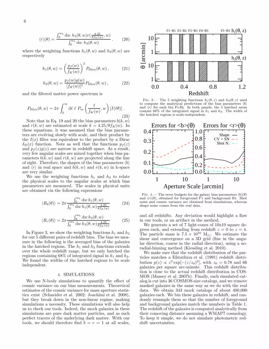
In Figure 3, we show the weighting functions h1 and h3

for our 5 different pairs of redshift bins. The bias we mea-sure in the following is the averaged bias of the galaxiesin the hatched regions. The h1 and h3 functions extendsover the whole redshift range, but we only hatched theregions containing 68% of integrated signal in h1 and h3.We found the widths of the hatched regions to be scaleindependent.

4. SIMULATIONS

We use N-body simulations to quantify the effect ofcosmic variance on our bias measurements. Theoreticalestimates of the cosmic variance for mass aperture statis-tics exist (Schneider et al. 2002; Joachimi et al. 2008),but they break down in the non-linear regime, makingsimulations a necessity. These simulations will also helpus to check our tools. Indeed, the mock galaxies in thesesimulations are pure dark matter particles, and as suchperfect tracers of the underlying dark matter. With ourtools, we should therefore find b = r = 1 at all scales,

1

10

F1−B1 F2−B2 F3−B3 F4−B3 F5−B3h1(θ, z)

0.0 0.4 0.8 1.2Redshift

1

10h3(θ, z)

θ [a

rcm

in]

Fig. 3.— The 5 weighting functions h1(θ, z) and h3(θ, z) usedto compute the analytical predictions of the bias parameters 〈b〉and 〈r〉 for each bin Fi-Bj. In both panels, the 5 hatched areascontain 68% of the integrated signal in h1 and h3. The width ofthe hatched regions is scale-independent.

Errors for <b>(θ)

1 100.0

0.1

0.2

0.3

0.4Errors for <r>(θ)

1 100.00.2

0.4

0.6

0.81.0

ShapeCV + SN

Shot N.

Aperture Scale [arcmin]Fig. 4.— The error budgets for the galaxy bias parameters 〈b〉(θ)

and 〈r〉(θ), obtained for foreground F1 and background B1. Shotnoise and cosmic variance are obtained from simulations, whereasshape noise comes from the real data.

and all redshifts. Any deviation would highlight a flawin our tools, or an artifact in the method.We generate a set of 7 light-cones of 10x10 square de-

grees each, and extending from redshift z = 0 to z = 4.The particle mass is 7.5 × 1010 M⊙. We estimate theshear and convergence on a 3D grid (fine in the angu-lar direction, coarse in the radial direction), using a no-radial-binning method (Kiessling et al. 2010).We make sure that the redshift distribution of the par-

ticles matches a Efstathiou et al. (1991) redshift distri-bution p(z) ∝ z2 exp[−(z/z0)

2], with z0 = 0.78 and 66galaxies per square arc-minute. This redshift distribu-tion is close to the actual redshift distribution in COS-MOS (Massey et al. 2007b). Finally, each simulated cat-alog is cut into 36 COSMOS-size catalogs, and we removemasked galaxies in the same way as we do with the realdata. We obtain 343 mock catalogs of about 400,000galaxies each. We bin these galaxies in redshift, and ran-domly resample them so that the number of foregroundand background galaxies match the numbers in Table 1.The redshift of the galaxies is computed analytically fromtheir comoving distance assuming a WMAP7 cosmology.To keep it simple, we do not simulate photometric red-shift uncertainties.

7

Figure 4 shows the error budget for the bias b andthe correlation coefficient r computed for the foregroundredshift bin F1, and the background bin B1. We split theerror budget into cosmic variance, shot noise and shapenoise. To quantify the uncertainty in our results dueto cosmic variance, we compute the bias parameters foreach COSMOS realization. The variance of the resultingdistribution is therefore due to cosmic variance and shotnoise. To quantify the amount of shot noise only, webootstrap the galaxies in one single COSMOS realization.As shown in Figure 4, we find the cosmic variance for

parameter 〈b〉 computed in foreground bin F1 and back-ground bin B1 to be larger than the shape noise. In con-trast for the correlation coefficient 〈r〉, shape noise dom-inates at all scales. 〈r〉 is more sensitive to shape noisebecause it contains the contributions from 〈N (θ)Map(θ)〉and 〈M2

ap(θ)〉, which are both affected by shape noise.We perform the same analysis with the other pairs inbins Fi-Bj, and find that shape noise is always largerthan cosmic variance both for bias parameters 〈b〉 and〈r〉. The reason is that background galaxies in bins B2and B3 are fainter, so their shape estimation is morenoisy.We also used the simulations to test our treatment

of the photometric redshift, and especially the way wereconstruct the weighting functions pb(z) and pf (z) forthe background and foreground redshift bins. We sim-ulated photometric redshifts with different redshift un-certainties from dz/(1 + z) = 0.01 to dz/(1 + z) = 0.05.We reconstructed the weighting functions of bins F1 andB1. For bin F1 with dz/(1 + z) = 0.05, we measuredthe rms between the recovered and the true p(z) to berms = 4.49± 0.32 for the standard histogram technique,and rms = 4.10 ± 0.33 for the sum of pdfs technique.For bin B1 with errors dz/(1 + z) = 0.01, we mea-sured rms = 0.48 ± 0.01 and rms = 0.65 ± 0.01 re-spectively. Therefore, our technique is better for largeredshift uncertainties, and lower redshift bins. In ourparticular case, where redshift uncertainties are aboutdz/(1 + z) = 0.05 for the faint part of the samples, ourtechnique is globally as good as constructing a standardhistogram of the best fit estimates. As already mentionedpreviously, we preferred this technique because galax-ies outside the redshift limits were properly taken intoaccount, which resulted in a better agreement betweenpredicted and observed signals. To push this compari-son further, more realistic galaxy redshift pdfs should besimulated, but this is out of the scope of this paper.Note finally that our estimates of the systematic er-

rors in our measurements of 〈b〉 and 〈r〉 might be un-derestimated because we do not consider scatter due toinaccurate photometric redshifts, and we do not popu-late the dark matter simulations with a realistic modelof galaxies. Therefore, any additional scatter introducedby physical processes involved in galaxy formation willnot be taken into account.

5. RESULTS

In this section, we present our measurements of the cor-relation functions. We use these measurements to derivethe bias, and estimate its scale- and redshift-dependence.

5.1. Correlation functions

As described in Appendix A, aperture statistics arecomputed from auto- and cross-correlation functions. Weuse the software Athena7, which implements a tree-code, and computes auto- and cross-correlation func-tions. For the tree-code, we choose an opening angle8

of 0.04 radians. All correlation functions are measuredin 950 logarithmic bins between 0.05 and 50 arc-minutes,which corresponds to a sampling scale of ∆ϑ = 0.007ϑ.The aperture statistics and the bias parameters are alsocomputed with this fine binning. We estimate the errorbars with bootstrapping, i.e. we repeat the measure-ments 200 times with different galaxy samples randomlydrawn from the input catalogs. For the figures, we rebinthe data in coarse bins using a median binning technique.We used the median rather than the mean because thedistributions of the bias parameters are not Gaussian,and so the median is more robust. However, this is asmall correction since with the mean instead, the biasparameters b and r would be only about 3% larger. Toallow a straightforward comparison, we use the same bin-ning for both the data and the simulations.In the following, we will always compare our results to

numerical predictions. We found the Smith et al. (2003)fitting formula to give a good approximation of the mea-surements at large scales. In contrast at small scales, wefound the fitting formula to under-predict the measure-ments (see e.g. Figures 6, 8 and 9). Hilbert et al. (2009)had already noticed this discrepancy at scales ℓ > 10000,and suggested that it could be due to the low resolutionof the simulations used by Smith et al. (2003). In ourcase, the discrepancies could at least partly also originatefrom the fact that we compare power-spectra of biasedgalaxy samples and dark-matter. Indeed, power-spectraof galaxies are expected to deviate from pure dark mat-ter power-spectra. Analyzing these deviations as a func-tion of scale, redshift and galaxy properties is in fact thewhole purpose of this paper. Therefore, comparing themeasured and the predicted measurements already giveus a first guess by eye of the amplitude of galaxy bias fora particular galaxy population.

Galaxy clustering— In Figure 5 we show the pro-jected galaxy auto-correlation function ω(θ) for our 5foreground redshift bins. We compute ω(θ) using theLandy & Szalay (1993) estimator defined as

ω(θ) =DD

RR− 2

DR

RR+ 1 . (26)

where the normalized numbers of pairs DD, RR and DRrefer to pairs of galaxy positions, random positions, andgalaxy and random positions respectively.By bootstrapping the data, we include shot noise in

the error bars for the data, and cosmic variance for thesimulations. At high redshift, we calculate smaller errorbars because (i) high redshift bins contain more galaxies,and (ii) we probe larger volumes and cosmic variance de-creases in larger volumes. In bins F4 and F5, we observe2σ and 3σ deviations respectively between the measured

7 http://www2.iap.fr/users/kilbinge/athena8 In Athena, galaxy properties are spatially averaged in nodes.

The opening angle between a central and a tangential node is theratio between the size of the tangential node divided by the distancebetween the nodes. The properties of two nodes are correlated ifthe opening angle is smaller than 0.04 rad.

8

0.01

0.10

1.00

ω(θ

)

F1

F2

1 10

0.01

0.10

1.00

ω(θ

)

F3

1 10

F4

1 10

F5

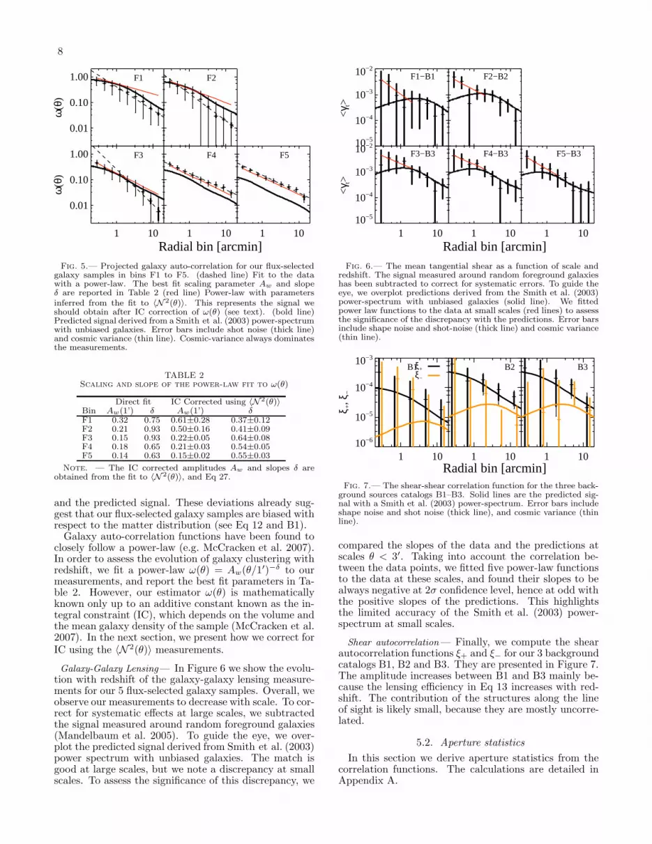
Radial bin [arcmin]Fig. 5.— Projected galaxy auto-correlation for our flux-selected

galaxy samples in bins F1 to F5. (dashed line) Fit to the datawith a power-law. The best fit scaling parameter Aw and slopeδ are reported in Table 2 (red line) Power-law with parametersinferred from the fit to 〈N 2(θ)〉. This represents the signal weshould obtain after IC correction of ω(θ) (see text). (bold line)Predicted signal derived from a Smith et al. (2003) power-spectrumwith unbiased galaxies. Error bars include shot noise (thick line)and cosmic variance (thin line). Cosmic-variance always dominatesthe measurements.

TABLE 2Scaling and slope of the power-law fit to ω(θ)

Direct fit IC Corrected using 〈N 2(θ)〉Bin Aw(1’) δ Aw(1’) δF1 0.32 0.75 0.61±0.28 0.37±0.12F2 0.21 0.93 0.50±0.16 0.41±0.09F3 0.15 0.93 0.22±0.05 0.64±0.08F4 0.18 0.65 0.21±0.03 0.54±0.05F5 0.14 0.63 0.15±0.02 0.55±0.03

Note. — The IC corrected amplitudes Aw and slopes δ areobtained from the fit to 〈N 2(θ)〉, and Eq 27.

and the predicted signal. These deviations already sug-gest that our flux-selected galaxy samples are biased withrespect to the matter distribution (see Eq 12 and B1).Galaxy auto-correlation functions have been found to

closely follow a power-law (e.g. McCracken et al. 2007).In order to assess the evolution of galaxy clustering withredshift, we fit a power-law ω(θ) = Aw(θ/1

′)−δ to ourmeasurements, and report the best fit parameters in Ta-ble 2. However, our estimator ω(θ) is mathematicallyknown only up to an additive constant known as the in-tegral constraint (IC), which depends on the volume andthe mean galaxy density of the sample (McCracken et al.2007). In the next section, we present how we correct forIC using the 〈N 2(θ)〉 measurements.

Galaxy-Galaxy Lensing— In Figure 6 we show the evolu-tion with redshift of the galaxy-galaxy lensing measure-ments for our 5 flux-selected galaxy samples. Overall, weobserve our measurements to decrease with scale. To cor-rect for systematic effects at large scales, we subtractedthe signal measured around random foreground galaxies(Mandelbaum et al. 2005). To guide the eye, we over-plot the predicted signal derived from Smith et al. (2003)power spectrum with unbiased galaxies. The match isgood at large scales, but we note a discrepancy at smallscales. To assess the significance of this discrepancy, we

10−5

10−4

10−3

10−2

<γ t>

F1−B1

F2−B2

1 1010−5

10−4

10−3

10−2

<γ t>

F3−B3

1 10

F4−B3

1 10

F5−B3

Radial bin [arcmin]Fig. 6.— The mean tangential shear as a function of scale and

redshift. The signal measured around random foreground galaxieshas been subtracted to correct for systematic errors. To guide theeye, we overplot predictions derived from the Smith et al. (2003)power-spectrum with unbiased galaxies (solid line). We fittedpower law functions to the data at small scales (red lines) to assessthe significance of the discrepancy with the predictions. Error barsinclude shape noise and shot-noise (thick line) and cosmic variance(thin line).

1 1010−6

10−5

10−4

10−3

ξ +, ξ

−

B1 ξ+ ξ−

1 10

B2

1 10

B3

Radial bin [arcmin]Fig. 7.— The shear-shear correlation function for the three back-

ground sources catalogs B1–B3. Solid lines are the predicted sig-nal with a Smith et al. (2003) power-spectrum. Error bars includeshape noise and shot noise (thick line), and cosmic variance (thinline).

compared the slopes of the data and the predictions atscales θ < 3′. Taking into account the correlation be-tween the data points, we fitted five power-law functionsto the data at these scales, and found their slopes to bealways negative at 2σ confidence level, hence at odd withthe positive slopes of the predictions. This highlightsthe limited accuracy of the Smith et al. (2003) power-spectrum at small scales.

Shear autocorrelation— Finally, we compute the shearautocorrelation functions ξ+ and ξ− for our 3 backgroundcatalogs B1, B2 and B3. They are presented in Figure 7.The amplitude increases between B1 and B3 mainly be-cause the lensing efficiency in Eq 13 increases with red-shift. The contribution of the structures along the lineof sight is likely small, because they are mostly uncorre-lated.

5.2. Aperture statistics

In this section we derive aperture statistics from thecorrelation functions. The calculations are detailed inAppendix A.

9

0.001

0.010

0.100<

Nap2

>F1

F2

1 10

0.001

0.010

0.100F3

1 10

F4

1 10

F5

Aperture Scale [arcmin]Fig. 8.— The galaxy aperture variance. To guide the eye, we

overplot the predicted signal derived from a Smith et al. (2003)power-spectrum with unbiased galaxies (solid line). As expectedthe prediction underestimates the signal at small scales. At largescales, the deviation in bins F4 and F5 already suggests that galax-ies are biased (see also Figure 11). Error bars include shot-noise(thick line), and cosmic variance (thin line).

Galaxy aperture variance— The measurements of〈N 2(θ)〉 for the 5 foreground bins are shown in Figure 8.For each redshift bin, we fit a power-law. In contrast toω(θ), 〈N 2(θ)〉 is not affected by IC, because the compen-sated filter T+ which multiplies ω(θ) in Eq A10 cancelsout any constant, including IC (Schneider et al. 1998).Simon et al. (2007) derived an analytic relation betweenthe parameters of a power-law fit to 〈N 2(θ)〉 and the pa-rameters of a PL fit to an IC corrected correlation func-tion ω(θ). The slope of ω(θ) corrected for IC is givenby

f(δ) = 0.0051δ11.55 + 0.2769δ3.95 + 0.2838δ1.25 , (27)

where δ is the slope of the PL fit to 〈N 2(θ)〉. The am-plitude of the PL fit to ω(θ) is the same as the ampli-tude of the PL fit to 〈N 2(θ)〉. In Table 2, we report theIC-corrected amplitudes Aw and slopes δ of the galaxyautocorrelation function ω(θ) obtained with Eq 27.We find that the amplitude Aw decreases with red-

shift, in agreement with McCracken et al. (2007) whoalso found smaller amplitudes for fainter galaxies in COS-MOS i.e. more likely located at higher redshift. Besides,we note a jump in amplitude between bins F3 and F2, i.e.between redshift z ∼ 0.52 and z ∼ 0.35. With respectto the slope δ, we observe a slight but not significant(less than 1σ) steepening with redshift. Such a pecu-liar behavior could be explained by the large scale struc-ture identified at redshift z ∼ 0.7 already detected inseveral other studies (Massey et al. 2007a; Guzzo et al.2007; Meneux et al. 2009; de la Torre et al. 2010). Weguess that more massive galaxies in this structure wouldincrease the slope because they are typically more clus-tered than average.Finally, we observe an increasing deviation (more than

5σ in bin F5) between the measurements and the signalpredicted with a Smith et al. (2003) power spectrum andunbiased galaxies. This suggests that galaxies are morebiased at high redshift, in agreement with expectations.

<N

Map

>

1x1

0−4 1

x10−

3 F1−B1

F2−B2

<N

Map

>

1x1

0−4 1

x10−

3 F3−B3

F4−B3

F5−B3

<N

Mx>

−4x

10−

4 4x1

0−4

1 10

<N

Mx>

−4x

10−

4 4x1

0−4

1 10

1 10

Aperture Scale [arcmin]

Fig. 9.— The galaxy-mass aperture covariance as a function ofscale and redshift. To guide the eye at large scale, we also show thepredictions derived from the Smith et al. (2003) power-spectrumwith unbiased galaxies (solid line). For bin F2-B2, we found thechange of slope of be not significant compared to a power-law fit(blue line). In red, 〈NMx〉 quantifies the amount of “B-modes”(see text). Error bars include shape noise (thick line) and cosmicvariance (thin line).

For bin F4 in the last 3 bins, we find on average a biasof about 1.4 between the data and the predictions, andfor bin F5 in the last 5 bins, we find a bias of about 2.6.

Galaxy-mass aperture covariance— The measurementsof 〈N (θ)Map(θ)〉 for our 5 foreground redshift bins areshown in Figure 9. In agreement with the < γt >measurements, we again note that a Smith et al. (2003)power-spectrum under-predicts the data points at smallscales. We performed a χ2-test, and found this disagree-ment to be significant in all bins at more than 3σ (weincluded the covariances matrices in the χ2-test). Thisdisagreement is also present for the stellar-mass selectedgalaxy samples in Figures 16 and 17. At small scales inbin F2-B2, we also note a slight change of slope at 1’scale. Again, we investigate the significance of this fea-ture with a χ2-test, but found a reduced χ2 = 1.60 whichis not enough to reject a simple power-law model.An E/B mode decomposition also exits for the

〈N (θ)Map(θ)〉 statistics. 〈NMx〉 quantifies the amountof B-modes in the measurement, and is computed by re-placing γt by γx in Eq A11. γx is the galaxy-galaxyclustering signal obtained with the coordinate system ro-tated by 45 degrees. This operation is commonly usedto reveal B-modes contamination if a 〈NMx〉 signal isdetected. Using a χ2-test and taking into account thecorrelation between the data points, we find the B-modesfor 〈NMx〉 to be consistent with zero in all bins Fi-Bj at95% confidence level, hence confirming a very low levelof contamination in our analysis.

Mass aperture variance— The measurements of 〈M2ap(θ)〉

for bins B1, B2 and B3 are shown in Figure 10. The solid

10

<

Map2

>

1

x10−

6 1

x10−

4

B1

B2

B3

1 10

1 10

1 10

Aperture Scale [arcmin]Fig. 10.— The mass-aperture variance as a function of scale and

redshift. To guide the eye, we overplot predictions derived fromthe Smith et al. (2003) power spectrum. In bin F2-B2, we fitteda power-law (blue line) to the data and found the change of slopeof be not significant. (in red) The “B-modes” are consistent withzero at all scales in all bins. Errors include shape noise and shotnoise (thick line), and cosmic variance (thin line).

0.1 1.0 10.0eff comoving scale [h−1 Mpc]

1

1

1

1

1

bias

<b>

0.5

0.51.5

0.51.5

0.51.5

0.51.5

1.5 F5−B3

F4−B3

F3−B3

F2−B2

F1−B1

Fig. 11.— Evolution of bias in comoving scale and redshift forthe flux-limited galaxy sample. Bias increases with redshift bothbecause flux-selected galaxies reside in more massive halos, and be-cause halos of any given mass are more biased at high redshift. Atsmall scales, the change of slope can be interpreted as the transi-tion between the two-halo and the one-halo terms in a halo modelframework. Errors bars include shape and shot noise (thick line),and cosmic variance (thin line). The horizontal dashed line marksthe value b = 1 for each bin. The data points are correlated (seeSection 5.6).

line represents the predicted signal with a Smith et al.(2003) power spectrum. We performed a χ2-test betweenthe data points and the predicted signal and found thatthe data points are consistent with the predicted signalat 68% confidence level for all bins B1, B2 and B3. Atall scales, shape noise dominates over cosmic variance.Errors are smaller for bin B3, because the signal is larger(about 10 times larger than the signal in bin B1).

5.3. Bias of the flux-selected sample

5.3.1. Constant bias model

In Figure 11, we show the galaxy bias 〈b〉(R) for oursample of flux-limited galaxies. We observe that bias

0.1 1.0 10.0eff comoving scale [h−1 Mpc]

01

02

1

02

1

02

1

02

1

2

bias

<b>

F5−B3

F4−B3

F3−B3

F2−B2

F1−B1

109 < M* < 1010

1010 < M* < 1011

Fig. 12.— Same as Figure 11, but for stellar-mass selected galax-ies. Bias increases with redshift and stellar-mass. The horizontaldashed line marks the value b = 1 for each bin.

varies with scale and redshift, but since the data pointsare correlated we use a χ2-test to quantify the signifi-cance of these variations. First, we assume the null hy-pothesis that bias is scale and redshift-independent. Totest this hypothesis, we fit a constant b0 to the 45 datapoints in the 5 redshift bins, and compute the χ2 statis-tics

χ2 = (B− b0)TC−1(B− b0) , (28)

where B is a vector containing the 45 data points, and Cis their covariance matrix. To perform the fit and find thebest fit parameters, we use the IDL AMOEBA technique(Nelder & Mead 1965), and repeat the process 100 timeswith different starting values. We obtain a best fit withχ2 = 229. Our data points are correlated, so the effectivenumber of degrees of freedom (dof) to perform the χ2 testis less than the number of data points N = 45 minusthe number of free parameters. Bretherton et al. (1999)proposed several estimators for the number of degreesof freedom for correlated data. We use the followingestimator9

dof =N2

∑

ij r2ij

(29)

where rij is the correlation coefficient between datapoints bi and bj, and N is the number of data points.Using this estimator, we find dof = 32 − 1 = 31, wherewe subtracted 1 for the parameter we fit. The reduced χ2

is therefore χ2/dof = 7.4, which allows us to confidentlyreject a constant bias model given our data.

5.3.2. Redshift-dependent model

Here we discuss a test of the redshift dependence ofbias. To our model, we add the following redshift depen-dence

9 Bretherton et al. (1999) mainly studied another estimatordof = (

∑i Cii)2/

∑ij C

2ij , which is equivalent if the data points

are centered and normally distributed with unit variance.

11

b(z) = b0 + b1z . (30)

We obtain a reduced χ2/dof = 2.5. Although still nota good fit, this model is nonetheless significantly betterthan the previous redshift-independent model.So far, we have ruled out a constant bias with redshift

and scale, but we did not isolate the redshift dependenceor scale dependence yet. This is the purpose of the restof this section.

5.3.3. Scale-independent model

Next, we test the scale-dependence only. Our null hy-pothesis is now that bias is scale-independent. For eachredshift bin, we fit a constant, and sum the χ2 for eachindividual redshift bin. We obtain a total χ2 = 43 for aneffective number of degrees of freedom dof = 32−5 = 27.This means that there are 97.4% chance that the scale-independent model is wrong. Here we subtracted 5 forthe 5 constant parameters we fit. A fit of this model tothe stellar-mass selected galaxy samples brings less strin-gent constraints, with χ2/dof = 1.49 and χ2/dof = 1.0for the low and high stellar-mass selected samples respec-tively.

5.4. Bias of the stellar-mass selected sample

In Figure 12, we show the galaxy bias 〈b〉 for twostellar mass-selected galaxy samples as a function ofscale and redshift. Previous studies have shown thatstellar-mass is a good tracer of halo mass (see e.g.Leauthaud et al. 2011b, and references therein), whichin turn parametrizes most of the bias models. In con-trast, flux-selected samples are more affected by selectioneffects. For instance, low surface brightness extendedgalaxies are systematically under represented becausethey tend to evade the magnitude cuts (Meneux et al.2009). Our stellar-mass selected samples should there-fore tell us more about halo properties.

5.4.1. Halo mass

First, we derive the average halo mass for our two sam-ples of galaxies. For this purpose, we fit the bias modelproposed by Tinker et al. (2010)

b(ν) = 1−Aνa

νa + δac+Bνb + Cνc , (31)

defined in terms of the peak height ν = δc(z)/D(z)σ(M),where δc(z) is the critical density for halo collapse(Weinberg & Kamionkowski 2003), D(z) is the growthfactor, and σ2(M) is the variance of the density fluc-tuations smoothed with a top-hat filter of size R =(3M/4πρm)1/3. The parameters of this fitting functionderive from fits to N-body simulations. They are A =1.0 + 0.24y exp(−(4/y)4), a = 0.44y − 0.88, B = 0.183,b = 1.5, C = 0.019 + 0.107y + 0.19 exp(−(4/y)4) andc = 2.4. We define the parameter y ≡ log10∆ for over-density ∆ = 200 times the cosmological mean density.Although this bias model is not explicitly a redshift-

dependent model, we make use of the fact that ν scaleswith redshift to test the redshift dependence of our mea-surements.

The Tinker et al. (2010) model is a halo bias model,i.e. it was calibrated on halo clustering measured in N-body simulations. In contrast, we measure galaxy clus-tering for stellar-mass selected galaxies. Using it to inferhalo mass implies the two following assumptions : (i)the dark-matter mass function is constant in the rangeof halo mass we consider (ii) there is only one galaxyper halo. The first assumption is valid because ourgalaxies are embedded in halos with peak height ν ∼ 1and mass log10(M/M⊙) ≤ 13, and the halo mass func-tion in this regime is almost flat (Sheth & Tormen 1999;Tinker et al. 2008). The second assumption holds in thelinear regime where most of the signal comes from theclustering of central galaxies.To overcome the problem of having data points at dif-

ferent redshifts, we fit a redshift-normalized peak heightparameter ν0, defined such that b(νi) = b(ν0/D(zi)),where zi is the redshift of a data point bi. Since thismodel is only valid in the linear regime, we only considerthe 16 data points at scales R > 2 h−1 Mpc. We findχ2 = 3.13 and χ2 = 4.93 for dof = 10.8 and dof = 11.2respectively for the low and high stellar-mass galaxy sam-ples. Therefore, the model proposed by Tinker et al.(2010) fits well our data.This implies that our measurements agree with an

increase of bias with redshift. In addition, we canderive the halo mass of our two stellar-mass selectedgalaxy samples. Indeed, the best fit values are ν0 =0.77+0.20

−0.31 and ν0 = 1.01+0.24−0.18 for the low and the

high stellar-mass samples respectively. To compareto Leauthaud et al. (2011b), we compute the peakheight estimator at redshift z = 0.37, νz=0.37 =ν0/D(0.37) = 0.93 and νz=0.37 = 1.21 for the low andhigh stellar-mass samples, respectively. This translatesinto 9.64 < log10(M200/h

−1M⊙) < 12.29, and 11.51 <log10(M200/h

−1M⊙) < 12.80, respectively. These re-sults are in very good agreement with Leauthaud et al.(2011b), when considering that our two stellar-mass se-lected samples range between 109 h−2M⊙ < M∗ <1010 h−2M⊙ and 1010 h−1M⊙ < M∗ < 1011 h−2M⊙.As a last check, we also fit the Sheth et al. (2001) biasmodel, and found similar results. The data are not strin-gent enough to distinguish the two models.In Figure 13, we show the evolution of bias with

redshift. The data points are averages of points atscales R > 2 h−1Mpc, and errors come from the re-spective total covariances matrices. The total covari-ance matrix is the sum of the data covariance matrixand the simulation covariance matrix. The shape noise,shot noise and cosmic variance are thus taken into ac-count. For comparison, we overplot the bias measured byKovac et al. (2009) (K09) with the zCOSMOS dataset,and by Marinoni et al. (2005) (M05) with the VLT VI-MOS Deep Survey (VVDS). The zCOSMOS dataset isthe same as ours but with galaxies brighter than I814 <22.5. The bias measured by K09 follows our high stellar-mass galaxy samples, whereas the bias measured by M05follows our low mass samples. We attribute the differ-ence in bias between the two measurements to differencesin galaxy selection functions.We found bias in bin F3-B3 for the high stellar-mass

galaxy sample to be larger than expected. Although thisdata point still agrees with the bias model predictions at

12

0.0 0.2 0.4 0.6 0.8 1.0Redshift

0

1

2

3Li

near

bia

s <

b>109 < M* < 1010

1010 < M* < 1011

zCOSMOSVVDS

Tinker et al. 2010

Fig. 13.— Redshift evolution of bias averaged on scales R >2 h−1Mpc for the two stellar mass selected galaxy samples. Er-ror bars include shape noise, shot noise (thick line) and cosmicvariance (thin line). Solid lines are the best fit predicted by theTinker et al. (2010) halo bias fitting function. At z = 0.37, thehalo masses predicted by the model are log(M200/h−1M⊙) = 11.58and log(M200/h−1M⊙) = 12.36 for the low and high stellar-mass selected galaxy samples. Green boxes are measurements inVVDS for a volume-limited (MB < −20 + 5 log h) galaxy sample(Marinoni et al. 2005). Pink boxes are measurements in zCOS-MOS for MB < −20 − z galaxies (Kovac et al. 2009).

95% confidence level, it shall be discussed further. In-deed at a similar redshift, K09 also identified a signifi-cant overdensity of galaxies which could explain the largebias value, but Finoguenov et al. (2007) identified veryfew massive groups. These two inconsistent observationsare puzzling. A halo model alike the one proposed byLeauthaud et al. (2011a) could help us understand bet-ter the peculiar properties of the galaxies at this redshift,in particular the fraction of satellite galaxies.

5.4.2. Scale-dependent model

In section 5.3, we showed that a scale-dependent biasmodel was preferred but still not significantly better thana scale-independent model. Nonetheless, we observe byeye that bias systematically decreases at small scales, andthe turn-down seems to start at scale R ∼ 2 h−1Mpc,which could correspond to the transition between theone-halo and the two-halo term, already identified in sev-eral previous papers. According to Zehavi et al. (2005),the behavior of bias at this transition scale is due topairs of satellite galaxies. With a halo model appliedto simulated data, Kravtsov et al. (2004) showed thata significant amount of pairs with satellite galaxies wascrucial for a smooth transition. Coupon et al. (2011),using the CFHT Lensing Survey, and Peng et al. (2011),with SDSS data, also found that the fraction of satel-lite galaxies depend on the overdensity and not on thehalo mass or redshift. Since overdensities increase at latetime, the number of satellite galaxies increases in low red-shift samples of galaxies. A change of slope in our data

TABLE 3Best fit parameters for the scale and redshift dependent

model (Eq. 32) applied to the109 h−2M⊙ < M∗ < 1010 h−2M⊙ (low) and

1010 h−2M⊙ < M∗ < 1011 h−2M⊙ (high) stellar-massselected samples.

LOW HIGH

RTD h−1Mpc 2.6± 1.2 1.0+0.8−0.2

α1 0.42+0.32−0.21 0.63± 0.18

α2 −0.17+0.44−0.41 −0.44± 0.24

logM200/h−1M⊙ 11.7+0.6−1.3 12.4+0.2

−2.9

χ2/dof 0.7 1.0

would therefore indicate a change of the satellite fractionin the galaxy samples.In order to measure the significance of an evolution of

the slope with redshift, we parametrize it as α(z) = α1+α2z. We also introduce a turn-down scale RTD beyondwhich bias evolves linearly. The final scale-dependentbias model we fit to the data is

b(R, z) = blin(ν)

(

RRTD

)α1+α2z

R < RTD

1 R ≥ RTD

. (32)

where we use the redshift-dependent bias model blin(ν)of Tinker et al. (2010) to describe the bias in the linearregime. We find χ2/dof = 0.7 and χ2/dof = 1.0 for thelow and high stellar-mass selected samples respectively.The best fit parameters are reported in Table 3.The difference in χ2 between the scale-independent

(SI) and scale-dependent (SD) model ∆χ2 = χ2SI/dofSI−

χ2SD/dofSD = 0.79 is not large enough to completely rule

out the SI bias model.The best fit parameters of the SD model merit some

particular attention. First, the scale at which biasturns down is detected to be between 0.8 h−1Mpc and3.8 h−1Mpc at 68% CL. In contrast to what was ob-served in SDSS (Johnston et al. 2007), the data suggestRTD to be marginally larger for less massive galaxies, butwe would need more bins in stellar-mass to confirm thistendency.Second, the slope of bias at scales below RTD is de-

tected to be larger than zero, but at less than 2σ CL.We measured α1 = 0.42+0.32

−0.21 and α1 = 0.63 ± 0.18for the low and high stellar-mass samples, respectively.Regarding its evolution with redshift, we found α2 =−017+0.44−0.41 for the low stellar mass galaxy sample,hence no significant evolution, but α2 = −0.44 ± 0.24for the high stellar-mass selected sample, hence a slightflattening of the slope at small scales at higher redshiftbins.It is expected that the steepness of the slope is related

to the occurrence of satellite galaxies in our sample, withmore satellite galaxies producing shallower slopes. Thecoincident fact that the turn-down scale is larger and theslope is shallower for the low stellar-mass sample suggestsa larger amount of satellite galaxies in our low stellar-mass selected sample.

5.5. Correlation coefficients

In Figure 14, we show the correlation coefficient 〈r〉for our flux-limited galaxy samples. Our measurements

13

eff comoving scale [h−1 Mpc]

co

rrel

atio

n <

r>

012

0

F5−B3<r> = 1.08±0.47

012

0

F4−B3<r> = 1.33±0.39

012

0

F3−B3<r> = 1.51±0.40

012

0

F2−B2<r> = 1.03±0.49

0.1 1.0 10.0012

0

F1−B1<r> = 0.58±0.28

Fig. 14.— The correlation coeffcient 〈r〉 measured in redshiftbins for our flux-limited galaxy samples. A deviation from r = 1suggests the bias relation is stochastic, and not perfectly linear.Our method produces artificial deviations from r = 1, which wequantify with pure dark matter simulations (pink area) for whichwe know a priori that r = 1. The size of the pink area is due tocosmic variance. The hatched area individuates the range of scaleswhere the simulations are consistent with r = 1. The averagedvalues of r are computed in these areas.

agree with r = 1 at all scales and all redshifts. Wenonetheless observe some trend in the data, that mightarise from possible artifacts in the method (see Sec-tion 6). To highlight them, we applied the method tothe simulated data, and indeed found a trend with a sig-nal greater than 1 at small scale and lower than 1 atlarge scale. We show the correlation coefficient and er-rors obtained from the simulations as pink regions. Con-sequently, the trends we observe in our data points can beexplained by artifacts in the method. The pink hatchedregions mark the scales where r is consistent with 1 in thesimulations. To compute the correlation factor for a par-ticular galaxy sample, we only average the data pointsin these regions.We found no significant deviation from r = 1, although

in bin F1-B1, we obtain r = 0.58± 0.28. Hoekstra et al.(2001) and Simon et al. (2007) found the correlation co-efficient 〈r〉 < 1 at 8σ, highlighting some stochasticity inthe bias relations of their galaxy samples. In our case,we can only say that our flux-selected and stellar-massselected samples are good tracers of the underlying massdistribution given the error bars (see also Figures 16 and17 for the results with the stellar-mass samples).We have found no standard halo model to predict the

scale-dependence of the correlation coefficient r. In con-trast, Neyrinck et al. (2005) propose a galaxy-halo modelwhich does. In their model, they assume halos attach togalaxies, in contrast to the standard halo model wheregalaxies attach to halos. By construction, assumingall halos have the same density profile, the correlation-coefficient is always r = 1. In the case halos have differ-ent density profiles, the correlation factor becomes scale

<b>(θ)

1 10Angular scale [arcmin]

1

10

Ang

ular

sca

le [a

rcm

in]

1 10

1

10

0.0

0.2

0.3

0.5

0.7

0.8

1.0<r>(θ)

1 10Angular scale [arcmin]

1

10

Ang

ular

sca

le [a

rcm

in]

1 10

1

10

0.0

0.2

0.3

0.5

0.7

0.8

1.0

Fig. 15.— Left : The correlation matrix of estimator 〈b〉(θ) fordata points in Figure 11 in bin F1-B1. Right : The correlationmatrix of estimator 〈r〉(θ) in Figure 14 in bin F1-B1. Both correla-tion matrices include shape noise, shot noise and cosmic variance.

dependent. At large scales, many halos are averagedover, resulting in a mean density profile. The matter dis-tribution therefore matches the galaxy distribution, andr = 1. At scales smaller than the minimum intergalacticdistance, r drops below 1 because of the many differentdensity profiles. Finally, assuming that the inner part ofthe density profiles are similar, r raises back to 1.In light of this model, we attempt to identify a dip

in bins F1-B1 and F2-B2 at scale R ∼ 2 h−1 Mpc.Hoekstra et al. (2002) and Simon et al. (2007) also ob-tained such a dip at scale R ∼ 1 h−1 Mpc with muchhigher significance. We fit a constant r = 1 to our datapoints in the hatched areas, and measured χ2 = 3.45in bin F1-B1 (dof = 2.75, > 68% CL at χ2 > 3.20),and χ2 = 2.20 in bin F2-B2 (dof = 3.06, > 68% CLat χ2 > 3.57). A constant model r = 1 therefore stillprovides a good fit to the data.

5.6. Bias correlation matrix

Figure 15 shows the correlation matrix of the bias(including cosmic variance) for the flux-limited galaxysample F1-B1. The data points are significantly corre-lated between 1’ and 10’ for the bias parameter 〈b〉, andless correlated for the correlation coefficient. The largeamount of correlation at the smallest scales θ < 0.4′ isdue to numerical artifacts (see section 6).Note as well that the large correlation between the an-

gular bins for parameter 〈b〉 only shows up when the co-variance matrix derived from simulations is added to thecovariance matrix derived from the data. Otherwise, theamount of correlation is weak because of the low signal-to-noise in the data. The signal to noise in the simulateddata is much higher, hence the stronger signal in the cor-relation matrix.

6. DISCUSSION

6.1. Artifacts in the measurements

It is well-known that aperture statistics, obtainedthrough integration of other estimators, are very sensi-tive to integration limits. Kilbinger et al. (2006) foundthat the signal is underestimated by more than 10% at12 times the lower integration limit, i.e. 0.6’ in our case.On the other hand, at large scales, the signal is only validup to half the upper scale limit (see Eq. 9–8). We usedsimulations to assess the systematic effects produced byaperture statistics. In Figure 16 and 17, our simulationsshow that the correlation coefficient 〈r〉 is overestimatedby 10% to 50% at scales θ < 1′, depending on the redshift

14

bin. For the bias parameter 〈b〉, deviations from b = 1occur at scales θ < 0.7′.In the simulations, we also observed that the cross-

correlation signals 〈N (θ)Map(θ)〉 and 〈γt〉 are biased lowat large scales. Subtracting the signal measured aroundrandom foreground did not help in recovering r = 1 atlarge scales. We found this effect to be less importantas the number of foreground galaxies decreases with re-spect to the number of background galaxies. This can beseen by comparing the red dashed lines in Figures 16 and17. Although this effect is of minor consequences on ourmeasurements given the size of the error bars, we tried tounderstand it. It is possible to demonstrate analyticallythat a constant additive systematic will cancel betweensources 90 degrees separated. When foreground galaxiesdo not have sources all around them or the additive sys-tematic is not constant, the average 〈γt〉 is biased low. Inthe Sloan Digital Sky Survey, Mandelbaum et al. (2005)found that subtracting the signal measured around ran-dom foreground galaxies was effectively removing thisnoise. However, our simulations do not include shapenoise, and therefore the signal we measure at large scalescannot be due to shape noise.Another source of systematic error could be related to

the tree-code we use to compute the correlation func-tions. The documentation for the tree-code Athenamentions that choosing a too large opening angle cansmear out the ellipticities of galaxies at large scales. In-deed, we find that if we increase the opening angle thenthe effect worsens, but it does not improve with valuessmaller than the one we use. Because this systematicerror is subdominant to our measurements, we decidednot to further attempt its correction.

6.2. Bin mismatch in redshift

In this section, we show that a mismatch in redshift be-tween peaks of the pf (z) and the lensing efficiency curvesg(z) can alter the bias measurements. We looked intothis issue because this is the case in bins F4-B3 and F5-B3. To understand the origin of the problem, we shouldrecall that in our method, the bias is the product of afunction f1 and a measurement 〈N 2(θ)〉/〈M2

ap(θ)〉.On the left panel of Figure 18, we compute the ra-

tios 〈N 2(θ)〉/〈M2ap(θ)〉 and the inverse of the functions

f1 for different combinations of foreground and back-ground sample bins. We find that between bins F1-B1and F1-B3 〈N 2(θ)〉/〈M2

ap(θ)〉 decreases by 37% and 33%at large and small scales respectively, whereas function f1decreases by 78% and 64%. As a result, our estimationsof bias change.We do expect the signal to decrease because 〈M2

ap(θ)〉increases with redshift, but we do not expect the mea-sured and the predicted signal to change by differentamounts. According to Eq 19, the bias measurementsshould only depend on the foreground redshift distribu-tion, and not on the choice of the background galaxysample and associated lensing efficiency. This is of courseassuming that 〈M2

ap(θ)〉 and the matter power spectrumgrows linearly, and the lensing-effective matter redshiftdistribution is well approximated by the lensing effi-ciency. For very wide surveys where many line of sightsare averaged over, the lensing efficiency might be a goodapproximation of the effective matter distribution, but

in COSMOS especially at low redshift, this might notbe the case. On the other hand at small scales in thenon-linear regime, the power spectrum might not growlinearly. In Figure 18, smaller scales are more affectedby bin mismatch.Given the limited size of the COSMOS field, we

therefore posit that cosmic variance or shape measure-ments could yield these discrepancies because the vol-umes probed by 〈M2

ap(θ)〉 are too small. This type ofdiscrepancies warn us that for future surveys, we shouldtry to match as closely as possible the mean redshift ofthe foreground galaxies and the peak of the lensing effi-ciency, in order to limit the effect of cosmic variance.

7. CONCLUSION

The strength of the COSMOS survey is the exceptionalquality of the ACS imaging, and the 30-band photome-try. Thanks to the latter, a photometric redshift can bederived for more than 600,000 galaxies at I814W < 26.0(Ilbert et al. 2009).In this paper we made use of these two properties to

investigate the evolution of stochastic bias with scaleand redshift in COSMOS. We partitioned our foregroundgalaxy catalogs in 3 categories : one flux-selected cat-alog (I814W < 26.5 and Ks < 24), and two stellar-mass selected catalogs. To estimate the bias parameterb and the correlation coefficient r, we applied a tech-nique based on aperture statistics described in (Schneider1998; Hoekstra et al. 2002). We used simulated lensingcatalogs derived from N-body simulations to quantifythe amount of error due to cosmic variance, and to testthe method against numerical artifacts. We found thatweak lensing shape noise dominates the error budget, andthat we are affected by some numerical artifacts at smallscales (θ < 0.6′), and at large scales for the correlationcoefficient r.Then, we used a χ2-test to assess the significance of

redshift evolution and scale-dependence of bias. Wefound a significant evolution of bias with redshift,but could not confidently rule out a scale-independentmodel. We found that both bias models proposed byTinker et al. (2010) and Sheth et al. (2001) provide agood fit to the redshift evolution of our measurementsat scales R > 2 h−1Mpc. We used the result of the fit toderive the halo mass of our stellar-mass selected galaxysamples. Finally, we observed that bias starts to declinebelow a scale of about 2 h−1Mpc. We proposed a biasmodel to describe this scale-dependence and obtained avery good fit with χ2/dof ≤ 1 for our two stellar-mass se-lected galaxy samples. We measured a 3σ significance ofthe turn-down scale RTD for the high stellar mass sam-ple, but could not draw conclusions about the evolutionof the slope with redshift because of low signal to noise.Finally, we observed that bias in bin F3-B3 is 2σ off the

expectations with a Tinker et al. (2010) bias model. Weattribute this to the presence of large over-densities in theCOSMOS field already identified in Kovac et al. (2009)and Massey et al. (2007a). With respect to bias stochas-ticity parameter 〈r〉, our measurements are all consistentwith 〈r〉 = 1. The linear bias model is therefore a goodfit to our data, albeit with somewhat large errors.The COSMOS field is still too small to produce deci-

sive conclusions about the evolution of bias, especiallyto characterize its scale-dependence, and to measure its

15

stochasticity in stellar mass-selected galaxy samples. Onaverage, we measured signal to noise ratios b/σb ∼ 3 andr/σr ∼ 0.5. The most important source of error is shapenoise in the background galaxies. Schneider et al. (1998)have shown that the error on 〈M2

ap(θ)〉 decreases as 1/Nb.In order to increase the signal to noise by a factor of 10,we would need a field 10 times larger.With their RCS and VIRMOS-DESCART survey of

50.5 deg2, Hoekstra et al. (2002) obtained signal to noiseratios about 8 on both bias parameters b and r. However,they did not perform simulations to disentangle system-atic and statistical errors as we did in this paper. Theyalso did not have redshift or stellar-mass estimates fortheir galaxies. Future ground-based wide field surveyssuch as KIDS and VIKING, DES, Pan-STARSS, LSSTand HyperSuprime-Cam on Subaru should provide goodphotometric redshifts and stellar-mass to perform a moreconclusive analysis of the scale- and redshift-dependenceof bias.The main challenge for weak-lensing tomography with

the future surveys (this bias analysis being one applica-tion) is to measure the shape of background galaxies upto redshift z = 4. This is essential to measure the red-shift evolution of galaxy properties and bias up to red-shift z ∼ 1. In their current implementation, the space-based missions Euclid and WFIRST propose a near-

infrared (NIR) and a visible channel (for Euclid), andvery wide field surveys. Visible and NIR imaging are crit-ical to produce good photometric redshifts (Jouvel et al.2011). These missions will also produce galaxy densitiesof about 30 per arc-minutes square. Therefore, with sev-eral millions of galaxies, they should be able to measurewith good S/N the scale-dependence of bias from verysmall to very large scales.

We would like to thank the referee for his insightfulcomments that led to a significant improvement of thepaper. It is also a pleasure to thank Chris Hirata andFabian Schmidt for useful discussions and helpful sug-gestions. We also gratefully thank Alexie Leauthaud forher help and advice, and for providing the COSMOSlensing catalog. This work was done in part at JPL,operated by Caltech under a contract for NASA. EJ ac-knowledges support from the Jet Propulsion Laboratory,in contract with the California Institute of Technology,and the NASA Postdoctoral Program. RM is supportedby an STFC Advanced Fellowship. c©2012. All rightsreserved.This work uses observations obtained with the Hubble

Space Telescope. The HST COSMOS Treasury programwas supported through NASA grant HST-GO-09822.

REFERENCES

Baldauf, T., Smith, R. E., Seljak, U., & Mandelbaum, R. 2010,Phys. Rev. D, 81, 063531

Bertin, E. & Arnouts, S. 1996, Astronomy & AstrophysicsSupplement, 117, 393

Blanton, M., Cen, R., Ostriker, J. P., & Strauss, M. A. 1999,ApJ, 522, 590

Bretherton, C., Widmann, M.and Dymnikov, V., Wallace, J., &Blade, I. 1999, Journal of Climate, 12, 1990

Bundy, K., Scarlata, C., Carollo, C. M., et al. 2010, ApJ, 719,1969

Capak, P., Aussel, H., Ajiki, M., et al. 2007, ApJS, 172, 99Coil, A. L., Newman, J. A., Croton, D., et al. 2008, ApJ, 672, 153Coupon, J., Kilbinger, M., McCracken, H. J., et al. 2011, ArXiv

e-printsCresswell, J. G. & Percival, W. J. 2009, MNRAS, 392, 682de la Torre, S., Guzzo, L., Kovac, K., et al. 2010, MNRAS, 1322Dekel, A. & Lahav, O. 1999, ApJ, 520, 24Efstathiou, G., Bernstein, G., Tyson, J. A., Katz, N., &

Guhathakurta, P. 1991, ApJ, 380, L47Eisenstein, D. J. & Hu, W. 1999, ApJ, 511, 5Finoguenov, A., Guzzo, L., Hasinger, G., et al. 2007, ApJS, 172,

182Guzzo, L., Cassata, P., Finoguenov, A., et al. 2007, ApJS, 172,

254Hilbert, S., Hartlap, J., White, S. D. M., & Schneider, P. 2009,

A&A, 499, 31Hoekstra, H., van Waerbeke, L., Gladders, M. D., Mellier, Y., &

Yee, H. K. C. 2002, ApJ, 577, 604Hoekstra, H., Yee, H. K. C., & Gladders, M. D. 2001, ApJ, 558,

L11Ilbert, O., Capak, P., Salvato, M., et al. 2009, ApJ, 690, 1236Joachimi, B., Schneider, P., & Eifler, T. 2008, A&A, 477, 43Johnston, D. E., Sheldon, E. S., Wechsler, R. H., et al. 2007,

ArXiv e-printsJouvel, S., Kneib, J.-P., Bernstein, G., et al. 2011, A&A, 532,

A25+Kiessling, A., Heavens, A. F., & Taylor, A. N. 2010, ArXiv

e-printsKilbinger, M., Schneider, P., & Eifler, T. 2006, A&A, 457, 15Koekemoer, A. M., Aussel, H., Calzetti, D., et al. 2007, ApJS,

172, 196Komatsu, E., Smith, K. M., Dunkley, J., et al. 2010, ArXiv

e-printsKovac, K., Porciani, C., Lilly, S. J., et al. 2009, ArXiv e-printsKravtsov, A. V., Berlind, A. A., Wechsler, R. H., et al. 2004,

ApJ, 609, 35Landy, S. D. & Szalay, A. S. 1993, ApJ, 412, 64

Leauthaud, A., Massey, R., Kneib, J.-P., et al. 2007, ApJS, 172,219

Leauthaud, A., Tinker, J., Behroozi, P. S., Busha, M. T., &Wechsler, R. 2011a, ArXiv e-prints

Leauthaud, A., Tinker, J., Bundy, K., et al. 2011b, ArXiv e-printsLilly, S. J., Le Brun, V., Maier, C., et al. 2009, ApJS, 184, 218Mandelbaum, R., Hirata, C. M., Seljak, U., et al. 2005, MNRAS,

361, 1287Marinoni, C., Le Fevre, O., Meneux, B., et al. 2005, A&A, 442,

801Massey, R., Rhodes, J., Ellis, R., et al. 2007a, Nature, 445, 286Massey, R., Rhodes, J., Leauthaud, A., et al. 2007b, ApJS, 172,

239Massey, R., Stoughton, C., Leauthaud, A., et al. 2010, MNRAS,

401, 371McCracken, H. J., Capak, P., Salvato, M., et al. 2010, ApJ, 708,

202McCracken, H. J., Peacock, J. A., Guzzo, L., et al. 2007, ApJS,

172, 314Meneux, B., Guzzo, L., de la Torre, S., et al. 2009, A&A, 505, 463Meneux, B., Le Fevre, O., Guzzo, L., et al. 2006, A&A, 452, 387Nelder, J. A. & Mead, R. 1965, Comput. J., 7, 308Neyrinck, M. C., Hamilton, A. J. S., & Gnedin, N. Y. 2005,

MNRAS, 362, 337Ouchi, M., Hamana, T., Shimasaku, K., et al. 2005, ApJ, 635,

L117Peacock, J. A. & Dodds, S. J. 1996, MNRAS, 280, L19Peng, Y., Lilly, S. J., Renzini, A., & Carollo, M. 2011, ArXiv

e-printsRhodes, J., Refregier, A., & Groth, E. J. 2000, ApJ, 536, 79Schneider, P. 1998, ApJ, 498, 43Schneider, P., van Waerbeke, L., Jain, B., & Kruse, G. 1998,

MNRAS, 296, 873Schneider, P., van Waerbeke, L., Kilbinger, M., & Mellier, Y.

2002, A&A, 396, 1Scoville, N., Aussel, H., Brusa, M., et al. 2007, ApJS, 172, 1Sheldon, E. S., Johnston, D. E., Frieman, J. A., et al. 2004, AJ,

127, 2544Sheth, R. K., Mo, H. J., & Tormen, G. 2001, MNRAS, 323, 1Sheth, R. K. & Tormen, G. 1999, MNRAS, 308, 119Simon, P. 2007, A&A, 473, 711Simon, P., Hetterscheidt, M., Schirmer, M., et al. 2007, A&A,

461, 861Smith, R. E., Peacock, J. A., Jenkins, A., et al. 2003, MNRAS,

341, 1311Somerville, R. S., Lemson, G., Sigad, Y., et al. 2001, MNRAS,

320, 289Tegmark, M. & Bromley, B. C. 1999, ApJ, 518, L69

16

Tinker, J., Kravtsov, A. V., Klypin, A., et al. 2008, ApJ, 688, 709Tinker, J. L., Robertson, B. E., Kravtsov, A. V., et al. 2010, ApJ,

724, 878van Waerbeke, L. 1998, A&A, 334, 1van Waerbeke, L., Bernardeau, F., & Mellier, Y. 1999, A&A, 342,

15Weinberg, N. N. & Kamionkowski, M. 2003, MNRAS, 341, 251Wild, V., Peacock, J. A., Lahav, O., et al. 2005, MNRAS, 356, 247

Yoshikawa, K., Taruya, A., Jing, Y. P., & Suto, Y. 2001, ApJ,558, 520

Zehavi, I., Eisenstein, D. J., Nichol, R. C., et al. 2005, ApJ, 621,22

Zehavi, I., Zheng, Z., Weinberg, D. H., et al. 2010, ArXiv e-printsZheng, Z., Zehavi, I., Eisenstein, D. J., Weinberg, D. H., & Jing,

Y. P. 2009, ApJ, 707, 554

APPENDIX

PRACTICAL ESTIMATORS

In practice, aperture statistics estimators are obtained from two point correlation functions (Schneider et al. 2002).The correlators used in this work are : (i) the angular correlation of the foreground galaxy positions, ω(θ), (ii) the meantangential shear about foreground galaxies, 〈γt〉(θ), (iii) the shear-shear correlation functions ξ±(θ) as determined fromthe ellipticities of the background galaxies (Simon et al. 2007) :The angular correlation of the foreground galaxy positions is computed with the Landy & Szalay (1993) estimator

defined as

ω(θ) =DD

RR− 2

DR

RR+ 1 . (A1)

The mean tangential shear around foreground galaxies is computed in angular scales, and is function of the shearcomponents γ1 and γ2

〈γt〉(θ)=⟨

w(i)γ(i,j)t ∆(i,j)(θ)

⟩

(A2)

=−⟨

w(i)(

γ(i)1 cos 2φ(i,j) + γ

(i)2 sin 2φ(i,j)

)

∆(i,j)⟩

where φ(i,j) = θ(i) − θ(j) is the polar angle between foreground galaxy i and background galaxy j. The angle bracketsstand for weighted mean over indices i and j and weights w(i). ∆(i,j)(θ) is a binning function

∆(i,j)(θ) =

1 for θ ≤ |θi − θj | < θ + δθ0 otherwise

(A3)

The shear-shear correlation functions ξ±(θ) are obtained from the correlation of the shear components γ1 and γ2 :

ξ+(θ) =⟨

w(i)w(j)γ(i)1 γ

(j)1

⟩

+⟨

w(i)w(j)γ(i)2 γ

(j)2

⟩

∆(i,j)(θ) (A4)

ξ−(θ) =(⟨

w(i)w(j)γ(i)1 γ

(j)1 cos 4φ(i,j)

⟩

−⟨

w(i)w(j)γ(i)2 γ

(j)2 cos 4φ(i,j)

⟩

+⟨

w(i)w(j)γ(i)1 γ

(j)2 sin 4φ(i,j)

⟩

+⟨

w(i)w(j)γ(i)2 γ

(j)1 sin 4φ(i,j)

⟩)

∆(i,j)(θ)

(A5)

Aperture statistics estimators can be expressed in terms of these correlators (Schneider et al. 2002; Hoekstra et al.2002). First, the E- and B-mode of the aperture mass variance 〈M2

ap(θ)〉 are obtained from the shear-shear correlationfunctions ξ±(θ)

〈M2ap(θ)〉 =

1

2

∫ 2θ

0

dϑ ϑ

θ2

(

ξ+(ϑ)T+

(

ϑ

θ

)

+ ξ−(ϑ)T−

(

ϑ

θ

))

, (A6)

〈M2⊥(θ)〉 =

1

2

∫ 2θ

0

dϑ ϑ

θ2

(

ξ+(ϑ)T+

(

ϑ

θ

)

+ ξ−(ϑ)T−

(

ϑ

θ

))

. (A7)

where

T+(x)=6(2− 15x2)

5

[

1− 2

πarcsin(x/2)

]

+x√4− x2

100π(120 + 2320x2 − 7544

+132x6 − 9x8) , (A8)

17

T−(x) =192

35πx3

(

1− x2

4

)7/2

. (A9)

T±(x) vanish for x > 2. The B-mode aperture mass 〈M2⊥(θ)〉 provides a quantitative estimate of the systematics,

since gravitational lensing only produces E-modes.Second, the aperture count variance 〈N 2(θ)〉 is related to ω(θ)

〈N 2(θ)〉 =∫ 2θ

0

dϑ ϑ

θ2ω(θ)T+

(

ϑ

θ

)

. (A10)

Finally, the galaxy-mass cross correlation aperture 〈N (θ)Map(θ)〉 is obtained from the mean tangential shear 〈γt〉(θ)

〈N (θ)Map(θ)〉 =∫ 2θ

0

dϑ ϑ

θ2〈γt〉(θ)F

(

ϑ

θ

)

(A11)

where the function F (x) has no analytic expression and also vanishes for x > 2

F (x) = 576

∫ 2

0

dt

tJ2(xt) [J4(t)]

2. (A12)

CORRELATORS

We have seen in Eq 8 – 10 that the aperture statistics 〈N 2(θ)〉, 〈M2ap(θ)〉 and 〈N (θ)Map(θ)〉 derive from their

respective power-spectra multiplied by the same filter function I(ℓθ) = J4(x)/x2. This filter is convenient because

it is very narrow in Fourier-space, and almost acts as a δD(x) function. When integrated over the power-spectra, itresults in very limited correlation between the Fourier modes. The aperture statistics are close approximations of thepower-spectra but in real space. There is almost a bijective relation between angular scales, and Fourier modes. As aresult, it is possible to combine the aperture statistics to derive the bias parameters as it is done in Fourier space.In practice, aperture statistics derive from the correlators ω(θ), 〈γt〉(θ) and ξ±(θ). Correlators also derive from the

power-spectra, but filtered by different filters, as shown below (Hoekstra et al. 2002)

ω(θ)= 〈δn(0)δn(θ)〉

=1

2π

∫ ∞

0

dℓ ℓ Pn(ℓ)J0(ℓθ) , (B1)

〈γt〉(θ)= 〈δn(0)γt(θ)〉

=1

2π

∫ ∞

0

dℓ ℓ Pκn(ℓ)J2(ℓθ) , (B2)

ξ±(θ)= 〈γt(0)γt(θ)〉 ± 〈γ×(0)γ×(θ)〉

=1

2π

∫ ∞

0

dℓ ℓ Pκ(ℓ)J0,4(ℓθ) , (B3)

Therefore, taking their ratio to derive the bias parameters is unreliable. Note as well that some filters alike the Beselfunction J0(x) act as low-pass filters. Many Fourier modes are mixed together into one angular scale. Consequently,the correlation between the different angular scales is large.

18

<N

ap2 >

1

x10−

2 1

x10−

1

0.1 0.2 0.6 1.7

F1

0.1 0.4 1.0 2.9

F2

0.2 0.5 1.4 4.0

F3

0.2 0.6 1.7 5.0

F4

0.3 0.8 2.3 6.7

F5

eff comoving scale [h−1 Mpc]

<N

Map

>

1x1

0−4 1

x10−

3

0.1 0.2 0.5 1.4

F1−B1

0.1 0.3 0.9 2.5

F2−B2

0.1 0.4 1.2 3.3

F3−B3

0.2 0.5 1.5 4.2

F4−B3

0.2 0.7 2.0 5.6

F5−B3

<N

Mx>

−4x

10−

4 4x1

0−4

012345

bias

<b>

0.1 0.2 0.6 1.7

F1−B1

0.1 0.4 1.0 2.9

F2−B2

0.2 0.5 1.4 4.0

F3−B3

0.2 0.6 1.7 5.0

F4−B3

0.3 0.8 2.3 6.7

F5−B3

1 10012345

corr

elat

ion

<r>

1 10

0.1 0.2 0.6 1.5

F1−B1

1 10

1 10

0.1 0.4 1.0 2.7

F2−B2

1 10

1 10

0.2 0.5 1.4 3.6

F3−B3

1 10

1 10

0.2 0.6 1.7 4.6

F4−B3

1 10

1 10

0.3 0.9 2.3 6.1

F5−B3

eff comoving scale [h−1 Mpc]

Fig. 16.— Overview of the most important estimators involved in the measurement of bias and stochasticity for the stellar mass selectedgalaxy sample in the range 109 < M∗ < 1010 h−2 M⊙. The black curve in the two upper panels is the theoretical prediction derivedfrom a Smith et al. (2003) power-spectrum, and it is meant to guide the eye at large scales. The discrepancies at small scales are expected(see text). The red dashed curves are the signals obtained in the simulations, which highlight numerical artifacts. Data points must beinterpreted with respect to these curves rather than b = 1 and r = 1.

19

<N

ap2 >

1x1

0−2

1x1

0−1

0.1 0.2 0.6 1.7

F1

0.1 0.4 1.0 2.9

F2

0.2 0.5 1.4 4.0

F3

0.2 0.6 1.7 5.0

F4

0.3 0.8 2.3 6.7

F5

eff comoving scale [h−1 Mpc]

<N

Map

>

1x1

0−4 1

x10−

3

0.1 0.2 0.5 1.4

F1−B1

0.1 0.3 0.9 2.5

F2−B2

0.1 0.4 1.2 3.3

F3−B3

0.2 0.5 1.5 4.2

F4−B3

0.2 0.7 2.0 5.6

F5−B3

<N

Mx>

−4x

10−

4 4x1

0−4

012345

bias

<b>

0.1 0.2 0.6 1.7

F1−B1

0.1 0.4 1.0 2.9

F2−B2

0.2 0.5 1.4 4.0

F3−B3

0.2 0.6 1.7 5.0

F4−B3

0.3 0.8 2.3 6.7

F5−B3

1 10012345

corr

elat

ion

<r>

1 10

0.1 0.2 0.6 1.5

F1−B1

1 10

1 10

0.1 0.4 1.0 2.7

F2−B2

1 10

1 10

0.2 0.5 1.4 3.6

F3−B3

1 10

1 10

0.2 0.6 1.7 4.6

F4−B3

1 10

1 10

0.3 0.9 2.3 6.1

F5−B3

eff comoving scale [h−1 Mpc]

Fig. 17.— Same as Figure 16, but for galaxies in the stellar mass range 1010 < M∗ < 1011.

20

0

50

100

150

0.1 0.2 0.5 1.3

F1−B1

0.1 0.3 0.8 2.2

F2−B1

0.2 0.4 1.1 3.0

F3−B1

0

50

100

150F1−B2

F2−B2

F3−B2

1 100

50

100

150F1−B3

1 10

F2−B3

1 10

F3−B3

eff comoving scale [h−1 Mpc]

Aperture Scale [arcmin]

( <

Nap2

> /

<M

ap2 >

)1/

2

012345

0.1 0.2 0.5 1.3

F1−B1

0.1 0.3 0.8 2.2

F2−B1

0.2 0.4 1.1 3.0

F3−B1

012345

F1−B2

F2−B2

F3−B2

1 10012345

F1−B3

1 10

F2−B3

1 10

F3−B3

eff comoving scale [h−1 Mpc]

Aperture Scale [arcmin]

bias

<b>

Fig. 18.— The effects of a mismatch between foreground (F1, F2, F3) and background (B1, B2, B3) redshift bins for the stellar massselected galaxy sample 109 < M∗ < 1010. Left panel — The bias parameter 〈b〉 not calibrated by function f1. The thick line is thecalibration signal 1/f1 computed assuming b = 1. Right panel — The bias parameter 〈b〉 calibrated by function f1.