Embed Size (px)
Citation preview

Cournot Competition and Endogenous FirmSize∗
Jason BarrRutgers University, Newark
Francesco SaracenoObservatoire Français des Conjonctures Économiques
January 2005Rutgers University Newark Working Paper #2005-001
Abstract
We study the dynamics of firm size in a repeated Cournot gamewith unkown demand function.We model the firm as a type of artificialneural network. Each period it must learn to map environmentalsignals to both demand parameters and its rival’s output choice. Butthis learning game is in the background, as we focus on the endogenousadjustment of network size. We investigate the long-run behavior offirm/network size as a function of profits, rival’s size, and the type ofadjustment rules used.
Keywords: Firm size, adjustment dynamics, artificial neural net-works, Cournot games
JEL Classification: C63, D21, D83, L13
∗An earlier version of this paper was presented at the 10th International Conferenceon Computing in Economics and Finance, July 8-10, 2004, University of Amsterdam. Wethank the session participants for their comments.
1

1 IntroductionIn this paper we explore firm size dynamics, with the firm modeled as atype of artificial neural network (ANN). Two firms/networks compete at twodifferent levels. The first level, which has been explored in detail in otherwork (Barr and Saraceno (BS), 2004; 2005), looks at Cournot competitionbetween two neural networks. In this paper, this level of competition isessentially in the background, while the main form of strategic interactionis in regards to firm size dynamics. The firm, while playing the repeatedCournot game, has to make long run decisions about its size, which affectsnot only its own profits, but those of its rival as well.Our previous research showed that firm size, which was left exogenous,
is an important determinant of performance in an uncertain environment.Here we reverse the perspective, taking as given both the learning processand the dependence of firm profit on size and environmental complexity, andendogenize firm size in order to investigate whether simple adjustment rulessucceed in yielding the optimal size (defined as the result of a best responsedynamics). The computational requirements needed to discover the optimalnetwork size may be quite expensive for the firm; and thus we explore lesscostly methods for adjusting firm size.In particular, we explore two types of adjustment rules. The first rule
(”the isolationist”) has the firm adjusting its size simply based on its last pe-riod profit growth. The second rule (”the imitationist”) has the firm adjust-ing its size if its rival has larger profits. Lastly we investigate firm dynamicswhen the firms use a combined rule.We explore how the two firms interact to affect their respective dynamics;
we also study how the adjustment rate parameters affect dynamics and longrun firm size. In addition, we investigate the conditions under which theadjustment rules will produce the Cournot-Nash outcome.To our knowledge, no other paper has developed the issue of long run
firm growth in an adaptive setting. Here we highlight some of the importantfindings of our work:
• In the isolationist case, firm dynamics is a function of both environ-mental complexity, initial size, rival’s initial size and the adjustmentrate parameter. The value of a firm’s long run size is a non-linear func-tion of these four variables. Ceteris paribus, we find, for example, thatfirms using a simple rule gives decreasing firm size versus increasing
2

complexity. In fact, a complex environment causes profit growth, andconsequently, firm growth, to be lower.
• In the imitationist case, firm dynamics is also a function of initial firmsize, initial rival’s size, complexity and the adjustment rate parameter.In such a case, increasing complexity will yield lower steady state sizes,though they are not necessarily the same for the two firms.
• Via regression analysis we measure the relative effects of the variousinitial conditions and parameters on long run dynamics. We find thatown initial size is positively related to long run size, rival’s initial sizehas a negative effect for small initial size, but positive effect for largerinitial sizes. The larger the adjustment parameters, the larger is thelong run size.
• Finally, we show that the simple dynamics that we consider very rarelyconverge to the ’best response’ outcome. In particular, the firm’s ad-justment parameter plays an important role in guaranteeing such aconvergence.
Our work relates to a few different areas. Our approach to using a neuralnetwork fits within the agent-based literature on information processing (IP)organizations (Chang and Harrington, forthcoming). In this vein, organiza-tions are modeled as a collection or network of agents that are responsiblefor processing incoming data. IP networks and organizations arise becausein modern economies no one agent can process all the data, as well as makedecisions about it. The growth of the modern corporation has created theneed for workers who are managers and information processors (Chandler,1977; Radner, 1993).Typical models are concerned with the relationship between the struc-
ture of the network and the corresponding performance or cost (DeCanio andWatkins, 1998; Radner, 1993; Van Zandt, 1998). In this paper, the networkis responsible for mapping incoming signals about the economic environmentto both demand and a rival’s output decision. Unlike other informationprocessing models, we explicitly include strategic interaction: one firm’s abil-ity to learn the environment affects the other firm’s pay-offs. Thus a firmmust locate an optimal network size not only to maximize performance fromlearning the environment but also to respond to its rival’s actions. In our
3

case, the firm is able to learn over time as it repeatedly gains experience inobserving and making decisions about environmental signals.A second area of literature that relates to our work is that of the evo-
lutionary and firm decision making models of Nelson and Winter (1982),Simon (1982) and Cyret and March (1963). In this area, the firm is alsoboundedly rational, but the focus is not on information processing per se.Rather, the firm is engaged in a myriad of activities from production, salesand marketing, R&D, business strategy, etc. As the firm engages in its busi-ness activities it gains a set of capabilities that cannot be easily replicated byother firms. The patterns of behavior that it collectively masters are knowas its ’routines’ (Nelson and Winter,1982). Routines are often comprised ofrules-of-thumb behavior: continue to do something if it is working, change ifnot.In this vein, firms in our paper employ simple adjustment rules when
choosing a firm size. In a world where there is an abundance of informationto process, and when discovering optimal solutions is often computationallyexpensive firms will seek relatively easier rules of behavior, ones that producesatisfactory responses at relatively low cost (Simon, 1982).
The rest of the paper is organized as follows. Section 2 discusses themotivation for using a neural network as a model of the firm. Then, in section3, we give a brief discussion of the set up of the model. A more detailedtreatment is given in the Appendix. Next, section 4 gives the benchmarkcases of network size equilibria. Sections 5 to 7 discuss the heart of thepaper—the firm size adjustment algorithms and the results of the algorithms.Finally, section 8 presents a discussion on the implications of the model andalso gives some concluding remarks.
2 Neural Networks as a Model of the FirmIn previous work (BS, 2002; 2005) we argued that information processing isa crucial feature of modern corporations, and that efficiency in performingthis task may be crucial for success or failure. We further argued that whenfocussing on this aspect of firm behavior, computational learning theory maygive useful insights and modelling techniques. In this perspective, it is usefulto view the firm as a learning algorithm, consisting of agents that follow aseries of rules and procedures organized in both a parallel and serial man-
4

ner. Firms learn and improve their performance by repeating their actionsand recognizing patterns (i.e., learning by doing). As the firm processesinformation, it learns its particular environment and becomes proficient atrecognizing new and related information.Among the many possible learning machines, we focussed on Artificial
Neural Networks as models of the firm, because of the intuitive mappingbetween their parallel processing structure and firm organization. Neuralnetworks, like other learning machines, can generalize from experience to un-seen problems, i.e., they recognize patterns. Firms (and in general economicagents) do the same: the know-how acquired over time is used in tacklingnew, related problems.What is specific about ANNs, as learning machines, is the parallel and
decentralized processing. ANNs are composed of multiple units processingrelatively simple tasks in parallel. The combined result of this multiplicityis the ability to process very complex tasks. In the same way firms are oftencomposed of different units working autonomously on very specific tasks, andare coordinated by a management that merges the results of these simpleoperations in order to design complex strategies.Furthermore, the firm, like learning algorithms, faces a trade-off linked to
the complexity of its organization. Small firms are likely to attain a ratherimprecise understanding of the environment they face; but on the other handthey act pretty quickly and are able to design decent strategies with smallamounts of experience. Larger and more complex firms, on the other hand,produce more sophisticated analyses, but they need time and experienceto implement their strategies. Thus, the optimal firm structure may onlybe determined in relation with the environment, and it is likely to changewith it. Unlike computer science, however, in economics the search for anoptimal structure occurs given a competitive landscape, which imposes timeand money constraints on the firm.In our previous work we showed, by means of simulations, that the trade-
off between speed and accuracy generates a hump-shaped profit curve infirm size (BS, 2002). We also showed that as complexity of the environmentincreases the firm size that maximizes profit also increases. These resultsreappeared when we applied the model to Cournot competition. Here, weleave the Cournot competition and the learning process in the background,and investigate how network size changes endogenously.
5
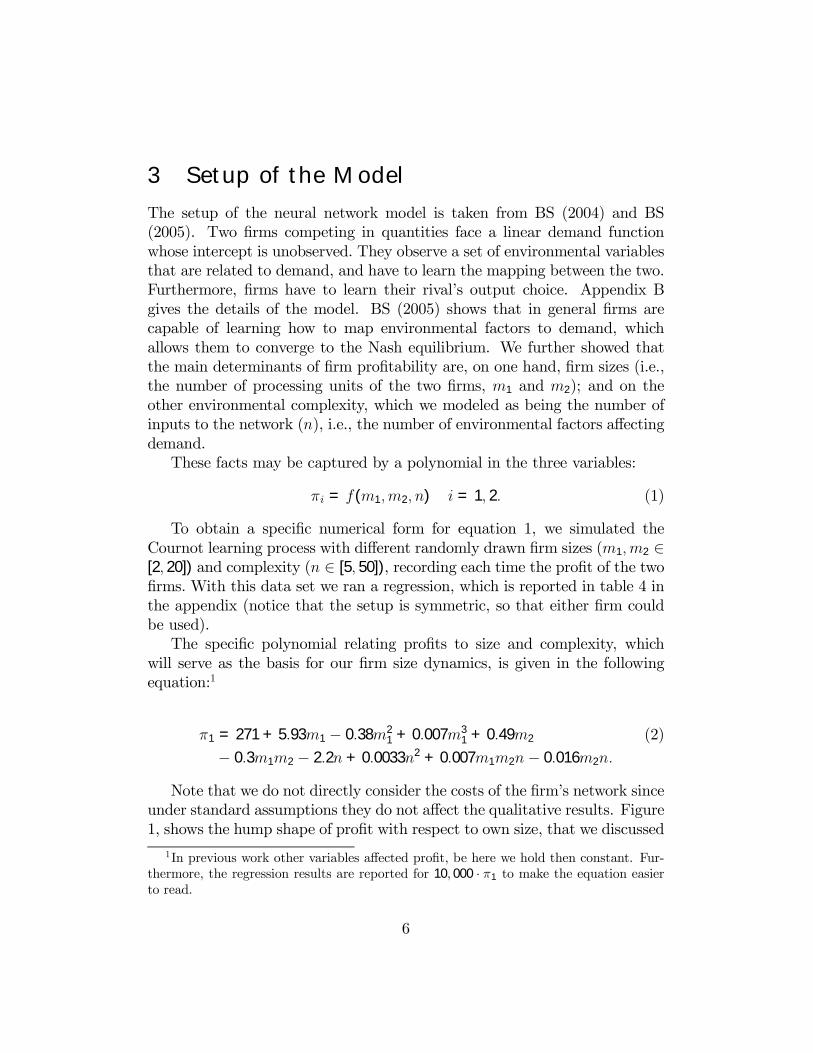
3 Setup of the ModelThe setup of the neural network model is taken from BS (2004) and BS(2005). Two firms competing in quantities face a linear demand functionwhose intercept is unobserved. They observe a set of environmental variablesthat are related to demand, and have to learn the mapping between the two.Furthermore, firms have to learn their rival’s output choice. Appendix Bgives the details of the model. BS (2005) shows that in general firms arecapable of learning how to map environmental factors to demand, whichallows them to converge to the Nash equilibrium. We further showed thatthe main determinants of firm profitability are, on one hand, firm sizes (i.e.,the number of processing units of the two firms, m1 and m2); and on theother environmental complexity, which we modeled as being the number ofinputs to the network (n), i.e., the number of environmental factors affectingdemand.These facts may be captured by a polynomial in the three variables:
πi = f(m1,m2, n) i = 1, 2. (1)
To obtain a specific numerical form for equation 1, we simulated theCournot learning process with different randomly drawn firm sizes (m1, m2 ∈[2, 20]) and complexity (n ∈ [5, 50]), recording each time the profit of the twofirms. With this data set we ran a regression, which is reported in table 4 inthe appendix (notice that the setup is symmetric, so that either firm couldbe used).The specific polynomial relating profits to size and complexity, which
will serve as the basis for our firm size dynamics, is given in the followingequation:1
π1 = 271 + 5.93m1 − 0.38m21 + 0.007m3
1 + 0.49m2 (2)
− 0.3m1m2 − 2.2n + 0.0033n2 + 0.007m1m2n− 0.016m2n.
Note that we do not directly consider the costs of the firm’s network sinceunder standard assumptions they do not affect the qualitative results. Figure1, shows the hump shape of profit with respect to own size, that we discussed
1In previous work other variables affected profit, be here we hold then constant. Fur-thermore, the regression results are reported for 10, 000 · π1 to make the equation easierto read.
6

in previous work. Three curves are reported, corresponding to small, mediumand large opponent’s size (complexity is fixed at n = 10).
200
220
240
260
280
prof1
2 4 6 8 10 12 14 16 18 20m1
Figure 1: A firm’s profit function vs. own size (m2 = 2, solid line; m2 = 10,crosses; m2 = 20, diamonds). n = 10.
4 The Best Response Function and NetworkSize Equilibrium
In this section, as a benchmark, we discuss the firm’s best response functionand equilibria that arise from the game. We can derive the best responsefunction in size by setting the derivative of profit with respect to size equalto zero, i.e.,
∂πi
∂mi
= f 0 (mi,m−i, n) = 0 i = 1, 2. (3)
Given the functional form for profit of equation (2), this yields the fol-lowing solution for firm 1 (as usual either firm can be used, as the problem
7

is symmetric)2:
mbr1 (m2, n) = 16.9± 2.26
√2.6m2 − 0.058nm2 + 3.9
The ’best response’ function is polynomial in mi and as a result, there isgenerally more than one solution, and often some of the solutions are complexnumbers. Nevertheless, for values of m2 and n in the admissible range (mi ∈[2, 20], n ∈ [5, 50]), the solution is unique and decreasing. The Network SizeEquilibrium (NSE) is given by the intersection of the best responses for thetwo firms. Figure 2 shows the best response mappings for equation (2), andthe corresponding Nash equilibria in size; notice that these equilibria arestable. In fact, in spite of the complexity of the profit function, the bestresponse is quasi-linear. Notice further the relationship between the bestresponses and environmental complexity: increasing complexity shifts thebest response functions, and consequently the Nash equilibrium upwards.In
4
5
6
7
8
9
10
11
12
m1
5 6 7 8 9 10 11 12m2
Figure 2: Best response functions (n = 10, diamonds; n = 25, crosses;n = 40, solid lines) for firms 1 and 2. The Network Size Equilibria are givenby the intersection of the lines.
general, we can express optimal firm size, m∗i , as a function of environmental
2For simplicity we ignore the integer issue in regards to firm size and assume that firmsize can take on any real value greater than zero.
8

complexity. If we take the two best responses, and we impose m∗1 = m∗
2 = m∗
by symmetry, we obtain the following:
m∗ = 23.5− 0.15n− 4.5p
(14.1− 0.34n + 0.001n2) (4)
The plot of this expression may be seen in figure 3.3
Finally, we can ask whether profits are increasing or decreasing at theequilibrium firm size. To answer this question, we substitute the optimalvalue given by equation (4) into the profit equation (2), to obtain a decreasingrelationship; the plot is also reported in figure 3.
200
220
240
260
280
5 15 25 35n
π
6
7
8
9
10
11
12
m*
Figure 3: Profit (solid line, left axis) at equilibrium is decreasing in environ-mental complexity. On the other hand, equilibrium size (crosses, right axis)is increasing.
To conclude, we have shown that best response dynamics yield a uniqueand stable equilibrium. Furthermore, we were able to show that the firm sizein equilibrium is increasing in complexity, while profit is decreasing. In thenext section we turn to simpler firm size adjustment rules, that require lowercomputational capacity for the firm.
3As was the case before, we actually have two solutions for firm size. Nevertheless, oneroot gives values that are outside the relevant range for m∗
, and can be discarded.
9

5 Adaptive Adjustment DynamicsAs discussed above, firms often face a large amount of information to process.In standard economic theory, firms are assumed to understand many detailsabout how the world functions and how various variables interact. They areassumed to know their cost functions, profit functions, and the effect of arival’s decisions on profits. But in a complex world, with boundedly rationalagents, the cost to discover such knowledge is relatively high. As a result,firms learn as they engage in their activities and use this knowledge to helpguide them.For this reason, in this section, we explore relatively simple dynamics for
firm size: dynamics that assume on the part of firms simply being able toobserve the effect that changing the number of agents (nodes) has on profits.The best response function in section 4 is quite complex, and assumed thatthe firm knows it; more specifically, it is assumed to know the expected max-imal profit obtainable for the entire range of a rival’s choice of network size.4
(Note also that the best response functions graphed above are numericalapproximations.)In addition in a world in which production and market conditions con-
stantly change, past information may quickly become irrelevant. Meaningthat even if a firm has perfect knowledge of its best response function ata certain point in time, that function may quickly become outdated. Thatmeans that even when the firm is in possession of the computational capabil-ities necessary to compute the best response, a firm may not find it efficientto actually do so.Using the profit function generated in section 3, we explore adjustment
dynamics for firms using rule-of-thumb type adjustment rules with the fol-lowing general adjustment dynamics:
mi,t = mi,t−1 + β (πi,t−1 − πi,t−2) + αIi [(m−i,t−1 −mi,t−1)(π−i,t−1 − πi,t−1)] .(5)
First, β represents the sensitivity of firm size to own profit growth. Inother words, if a firm has positive profit growth it will increase its firm sizeby β (πi,t−1 − πi,t−2), units; if profit growth is negative, it will decrease byβ (πi,t−1 − πi,t−2) . Again, we assume that firm size can take on a real-valued
4A common assumption in game theory is that firms know the equilbrium and thatthey know that their rival knows it, and they know that their rival knows they know it,ad infitinum (Fudenberg and Tirole, 1996).
10

positive number.Next, the parameter α captures the ”imitation” factor behind size ad-
justment; Ii is an indicator function taking the value of 1 if the opponent’sprofit is larger than the firm’s, and a value of 0 otherwise:
Ii =
½1 ⇔ (π−i,t−1 − πi,t−1) > 00 ⇔ (π−i,t−1 − πi,t−1) ≤ 0
In case Ii = 1, then size will be adjusted in the direction of the opponents’.Thus, the firm will adjust towards the opponent’s size, whenever it observes abetter performance of the latter (note that we do not have any discounting).To sum up, our adjustment rule only uses basic routines: first, the firm
expands if it sees its profit increasing; second it adapts towards the opponent’ssize whenever it sees that the latter is doing better. These are the mostbasic and commonsensical routines a firm would employ, and require verylittle observation and computation on the part of the firm. In short, we canthink of the Cournot game as happening on a short term basis, while theadjustment dynamics occurs over longer periods of time.In the next section we investigate the following questions: what kinds
of firm dynamics can we expect to see given the simple adjustment rules?And under what parameter choices using equation (5) will firms reach theequilibrium level presented in figure 3 and, what kinds of behavior can weexpect for firm size as a function of the parameter space?
6 Results
6.1 Scenario 1: The Isolationist Firm
Suppose that α = 0. Then each firm will only look at its own past perfor-mance when deciding whether to add or to remove nodes:
mi,t = mi,t−1 + β [πi,t−1(mi,t−1,m−i,t−1, n)− πi,t−2(mi,t−2,m−i,t−2, n)]
Of course, this does not mean that the firm’s own dynamics is independentof the other, as in fact πi,t−1 and πi,t−2 depend on both sizes. Figure 4 showsthe adjustment dynamics of two isolationist firms for different complexitylevels. The adjustment rate β is kept fixed (at β = 0.05).The dynamics are relatively simple and show a few things. The first is
that the long-run level, in general, is reached fairly quickly. The second is
11

10
15
20
25
30
35
0 1 2 3 4 5 6Time
Firm
siz
e
n=5
n=20
n=40
Figure 4: Firm dynamics when the firms start at different sizes (m1(0) = 10;m2(0) = 20), for three different levels of complexity.
that this level seems to depend on initial own size. For example, a firmstarting at say 10 nodes will converge at a value around 17-18 nodes; boththe opponent’s initial size, and the complexity level seem to have a verylimited effect, if any. These qualitative features do not change for differentinitial conditions (other figures available upon request). This result is hardlysurprising regarding the opponent’s size if we consider that the two firmshave a simple adjustment rule, so that interaction only takes place indirectly,through the profit function.Thus, at first sight the picture does not show strong differences in long
run dynamics. However a deeper look will show that initial size, initial rival’ssize complexity and β all have statistically significant effects on long run size.In section 6.3 below we show regression results for the dynamics of equation(5), where it appears that n and β are important determinants of long runsize. Thus, we conclude that in figure 4 the effects of these parameters arehidden by the predominant effect of initial size.Finally, figure 5 shows the adjustment dynamics for three different values
of β.When β = 0.025, firm size adjusts to approximately 15, when β = 0.075,long run firm size is larger, finally when β = 0.125, we see that long run firmsize is the largest (about 25) and that there are oscillatory dynamics, withdecreasing amplitude, but with apparently regular frequency. Thus we cansee that a larger β leads to larger long run firm size.
12

0
10
20
30
40
50
1 3 5 7 9 11 13 15 17 19 21 23 25 27 29 31 33 35 37 39 41
β=0.025 β=0.075 β=0.125
time
m1
Figure 5: m1(0) = m2(0) = 10, n = 20, three different β.
6.2 Scenario 2: The Imitationist
In this case the contrary of the isolationist firm holds: firms do not care abouttheir own situation, but rather about the comparison with the opponent:β = 0. Thus,
mi,t = mi,t−1 + αIi [(m−i,t−1 −mi,t−1)(π−i,t−1 − πi,t−1)] .
In this case, the firm will not change its size if it has a larger profit, and itwill adjust towards the opponent if it has a smaller profit. Thus, we can saya number of things before feeding actual parameter values. First, at eachperiod, only one firm moves. Second, at the final equilibrium, the two profitsmust be equal, which happens when firm sizes are equal, but not necessarilyonly in this situation. For n = 5, suppose one firm begins small and theother large (m1 = 4 and m2 = 15). The resulting dynamics depend on α, asshown in figure 6.For low levels of α, in fact, the drive to imitation is not important enough,
and the two firms do not converge to the same size. For intermediate values(around α = 0.125), instead, convergence takes place to an intermediate size.When α is too large, on the other hand, the initial movement (in this caseof firm 1) is excessive, and may overshoot.Complexity has a role as well, as shown in figure 7 (where n = 40). In
fact, as greater complexity yields larger firm size, we see that the adjustmentis faster (for each given α), and that for large enough values of α, the systemexplodes.
13

5 10 15 20 25 300
5
10
15
20α=0.025
m1m2
5 10 15 20 25 300
5
10
15
20α=0.075
m1m2
5 10 15 20 25 300
5
10
15
20α=0.125
m1m2
5 10 15 20 25 300
5
10
15
20α=0.175
m1m2
Figure 6: Firm dynamics for different values of α. n = 5.
Both in the imitationist and in the isolationist cases, the dynamics showa very strong dependence on initial conditions. This feature of the time seriescalls for a systematic analysis of the parameter space and we present belowregression results for the combined scenario.
6.3 Scenario 3: Combined Dynamics Regression Analy-sis
In this section, we investigate via regression analysis the effects of initialfirm size, adjustment parameters and complexity on long run firm size. Herewe combine the two types of dynamics, exploring the outcomes based onequation 5. To do this we generate 5, 000 random combinations of initial firmsizes from mi (0) ∈ {2, 20} , α ∈ [0.025, 0.075] , β ∈ [0.025, 0.075] and n ∈{5, 10, ...., 40} and then we look at the long run steady state firm size for firm1, which ranges from 2.6 to 39.6 nodes. The regression results are presentedin table 1. The regression equation is non-linear in the variables and includesseveral interaction terms. Also a dummy variable, δ [m1 (0) > m2 (0)] = 1 if
14

5 10 15 20 25 300
5
10
15
20α=0.025
m1m2
5 10 15 20 25 300
5
10
15
20α=0.075
m1m2
5 10 15 20 25 300
5
10
15
20
25α=0.125
m1m2
5 10 15 20 25 300
20
40
60
80
100α=0.175
m1m2
Figure 7: Firm dynamics for different values of α. n = 40.
m1 (0) > m2 (0) and 0 otherwise, was included since it was found to bestatistically significant.Column (4) of table 1 also includes coefficients for the normalized vari-
ables, which all have mean of zero and standard deviation of one. Thesecoefficients then allow us to compare the relative magnitudes of the variableson the dependant variable.>From the regression table we can draw the following conclusions:
• Increasing initial own firm size, increases long run size, and increasingrival’s size initially has a negative effect, but for m2 (0) > 8, the effectis positive.
• The parameters α and β both have positive effects on firm size, thoughnegative interaction effects with initial size.
• The dummy variable, which reflects the relative starting position of thetwo firms, shows that relative initial size matters in determining long
15

Dependent Variable: m1(100)
Variable Coef. Std. Err. Norm. Coef.m1 (0) 0.517 0.032 0.475[m1 (0)]2 0.009 0.001 0.190m2 (0) -0.289 0.030 -0.264[m2 (0)]2 0.031 0.001 0.632m1 (0) ·m2 (0) -0.020 0.001 -0.308δ [m1 (0) > m2 (0)] 0.447 0.090 0.038α 58.159 3.763 0.208β 159.342 4.536 0.569α ·m1 (0) -3.110 0.310 -0.175β ·m1 (0) -2.042 0.289 -0.114β ·m2 (0) 3.907 0.309 0.216n -0.040 0.008 -0.077n · β 1.401 0.125 0.163n ·m1 (0) 0.006 0.001 0.170Constant 3.157 0.301 .Nobs. 5000R2 0.878
Table 1: Regression results for adjustment dynamics. Dep. Var. m1(100).Robust standard errors given. All variables stat. sig. at 99% or greaterconfidence level.
run size. If firm 1 starts larger than firm two, all else equal, it will havea larger long run size.
• Ceteris paribus, increasing complexity is associated with smaller firmsize. The reason is that greater environmental complexity reduces prof-its and thus in turn reduces the long run size.
• However, there are several interaction effects that capture the non-linear relationship between the independent variables and long run firmsize. For example, both initial own size and the adjustment parametershave positive effects, but there are also off-setting interaction effectsthat reduce the total effect of starting size and the adjustment parame-ters. That is to say, the interaction variables, α ·m1 (0) and β ·m1 (0)have negative effects, while n · β has a positive effect. Interestingly,
16

n · α has no statistically significant effect on long run size (coefficientnot included).
7 Convergence to Nash EquilibriumAs we saw in the previous section, the long run size of the firm is determinedby several variables and, as a result, the convergence to the Nash equilib-rium is not guaranteed by the simple adaptive dynamics that we study inthis paper. As a result, this section investigates the conditions under whichconvergence takes place.We made random draws of the relevant parameters (α and β in the range
[0, 0.2], m1(0) and m2(0) in, the range [2, 20]), and we ran the dynamics.Then, we retained only the runs that ended up with both firms within onenode of the Nash value (i.e. mi(50) ∈ [m∗−0.5, m∗+0.5]. That was done onemillion times for each complexity value n ∈ {5, 10, 15, 20, 25, 30, 35, 40, 45}.Table 2 shows the results, reporting the success rate, the average α, β,
and initial m1, and the mode of the latter (given the symmetric setting, thevalues for m2(0) are identical). The numbers in parenthesis are the standarddeviations.
n (m∗) Succ. α β m1(0) mod[m1(0)]5 (6.85) 0.492% 0.122
(0.052)0.082(0.042)
8.758(5.380)
5
10 (7.19) 0.413% 0.115(0.057)
0.087(0.056)
7.897(5.267)
4
15 (7.58) 0.296% 0.093(0.056)
0.082(0.075)
4.137(1.476)
5
20 (8.01) 0.190% 0.106(0.053)
0.009(0.007)
4.845(1.792)
5
25 (8.53) 0.207% 0.106(0.054)
0.011(0.007)
4.972(1.896)
5
30 (9.15) 0.247% 0.105(0.053)
0.012(0.008)
5.408(2.137)
5
35 (9.91) 0.293% 0.105(0.053)
0.014(0.010)
5.700(2.347)
6
40 (10.93) 0.354% 0.110(0.050)
0.016(0.011)
6.304(2.583)
5
45 (12.50) 0.356% 0.119(0.048)
0.021(0.014)
6.967(2.948)
6
Table 2: Convergence to Nash equilibrium for different complexity levels
17

The first result that emerges is that only a very small number of runs con-verged close to the Nash value. In fact, the success ratio does not even attainhalf of a percentage point. The value was particularly low for intermediatecomplexity values. Thus, we find that even extremely simple and common-sensical adjustment rules, while allowing for convergence to a steady statevalue, do not yield the equilibrium ’full information’ outcome. This resultcalls for a careful assessment of the conditions under which a Nash outcomemay be seen as a plausible outcome.Another striking result is that the mode of the initial size is in fact in-
sensitive to complexity, whereas the mean has a slight u-shape (i.e., largervalues at the extremes of the complexity range). Thus, with respect to bothstatistics, we do not observe that the increase in complexity, and in the as-sociated Nash value for firm size, requires larger initial firms for convergenceto happen.In fact, from the table we can induce that the only variable that seems
to vary significantly with complexity is the profit coefficient β. The othersare quite similar across complexity values, both regarding the value and thestandard deviation.To further investigate the relationship between the exogenous variables
and the likelihood of the system settling down to a Nash equilibrium, weconducted a probit regression analysis. We created data set of 50, 000 obser-vations from random draws of the relevant parameters from the respectiveparameter sets given above. The probit analysis allows us to measure howthe parameters affect the probability that the system will reach a Nash equi-librium. The results of this regression are given in table 3, where we reportthe results of the marginal changes in probability with a change in the inde-pendent variable. A few conclusions can be drawn from the table:
• The probability of firm size reaching a Nash equilibrium is decreasingwith environmental complexity. This is quite intuitive, as more complexenvironments have a perturbing effect on the dynamics
• Cet. par. larger α is associated with a higher probability of reachingNash. This is due to the fact that the α parameter reflects the firminteraction with the opponent, and thus may be a proxy for a bestresponse dynamics. The more important this factor in the adjustmentdynamics, the greater the chances to mimic the best response dynamics.
18

Variable dF/dx std. err.n -0.00015 3.51E-05n2 2.90E-06 6.55E-07α 0.0046 0.0014β -0.0583 0.0072β2 0.170 0.028m1 (0) -0.00039 5.66E-05m2 (0) -0.00039 5.58E-05β ·m1 (0) 0.00089 0.00024β ·m2 (0) 0.00047 0.00019m1 (0) ·m2 (0) 0.000022 3.65E-06nobs. 50,000prob(Nash) 0.0033
\prob(Nash) .00076 (at x)pseudo R2 0.243
Table 3: Probit regressions results. Dep. var. is 1 if long run firm size isequal to Nash equilibrium, 0 otherwise. Robust standard error are presented.All coefficients are stat. sig. at 99% or greater confidence level.
• β has a quadratic relationship: having a negative effect for small betasbut increasing for values of β above 0.325.
• Initial firm size matters; the larger the initial size the lower the prob-ability of hitting the Nash equilibrium; though there are positive, off-setting interaction effects between own and rivals sizes.
• Lastly there is a positive interaction effect between β and initial ownand rival’s size.
8 Discussion and ConclusionThis paper has presented a model of the firm as an artificial neural network.We explored the long run size dynamics of firms/neural networks playing aCournot game in an uncertain environment. Building on previous paperswe derived a profit function for the firm that depends on its own size, therival’s size and environmental complexity. We then looked at long-run firm
19

size resulting from two types of simple adaptive rules: the ’isolationist’ andthe ’imitationist.’ These dynamics were compared to a benchmark ’bestresponse’ case.First we find that when using simple adjustment rules, long run firm size
is a function of initial firm size, initial rival’s size, environmental complexityand the adjustment rate parameters. These variables interact in a non-linearway. We also find that only under only very precise initial conditions andparameter values does the firm converge to the Nash equilibrium size givenby the best response. The reason is that the dynamics we consider tend tosettle rapidly (no more than a few iterations) on a path that depends oninitial conditions. The simple rules generally yield suboptimal long run equi-libria, and only fairly specific combinations of parameters and initial sizesyield the optimal size. Thus, our results suggest cautiousness in taking theNash equilibrium as a focal point of simple dynamics (the standard ’as if’argument). Interestingly, we further find that when firms use simple adjust-ment rules, environmental complexity has a negative effect on size, even ifthe Nash equilibrium size is increasing in environmental complexity. Thisis particularly true in the isolationist case, and is explained by the nega-tive correlation between profits and complexity: complex environments yieldlower profits, and hence less incentives for firm growth; ceteris paribus, thisyields lower steady state size, and suboptimal profits. Thus, in our modelmore efficient information processing, and more complex adjustment ruleswould play a positive role in the long run profitability of the firm, and woulddeserve investment of resources. It may be interesting to build a model inwhich firms face a trade-off between costs and benefits of costly but efficientadjustment rules.Finally, we found that β, the effect of own profit on firm size, is more
important than the comparison with the rival’s performance in determiningwhether the Nash outcome is reached or not. In fact, it emerged from ouranalysis that values of β in particular ranges significantly increased the prob-ability of convergence to the optimal size. This result triggers the question ofwhy such a parameter should be considered exogenous. One could imaginea ’superdynamics’, in which firms adjust their reactivity to market signals,i.e., their β, in order to maximize the chances of converging to the optimalsize. Such an investigation may also be the subject of future research. Otherextensions may include to link the findings with these models to stylized factsaround firm growth and size (i.e., the literature on Gibrat’s Law).
20

Appendix
A Neural NetworksThis appendix briefly describes the working of Artificial Neural Networks..For a more detailed treatment, the reader is referred to Skapura (1996).Neural networks are nonlinear function approximators that can map virtu-ally any function. Their flexibility makes them powerful tools for patternrecognition, classification, and forecasting. The Backward Propagation Net-work (BPN), which we used in our simulations, is the most popular networkarchitecture. It consists in a vector of x ∈ Rn inputs, and a collection of mprocessing nodes organized in layers.For our purposes (and for the simulations) we focus on a network with
a single layer. Inputs and nodes are connected by weights, wh ∈ Rn×m,that store the knowledge of the network. The nodes are also connected toan output vector y ∈Ro, where o is the number of outputs (2 in our case),and wo ∈ Rm×o is the weight vector. The learning process takes the formof successive adjustments of the weights, with the objective of minimizinga (squared) error term.5 Inputs are passed through the neural network todetermine an output; this happens through transfer (or squashing) functions,such as the sigmoid, to allow for nonlinear transformations. Then supervisedlearning takes place in the sense that at each iteration the network outputis compared with a known correct answer, and weights are adjusted in thedirection that reduces the error (the so called ‘gradient descent method’).The learning process is stopped once a threshold level for the error has beenattained, or a fixed number of iterations has elapsed. Thus, the working ofa network (with one hidden layer) may be summarized as follows. The feedforward phase is given by
y1×o
= g
·g
µx
1×n· wh
n×m
¶wo
m×o
¸where g(·) is the sigmoid function that is applied both to the input to the hid-den layer and to the output. To summarize, the neural network is comprisedof three ’layers’: the environmental data (i.e., the environmental state vec-tors), a hidden/managerial layer, and an output/decision layer. The ’nodes’
5The network may be seen as a (nonlinear) regression model. The inputs are the inde-pendent variables, the outputs are the dependent variables, and the weights are equivalentto the regression coefficients.
21

in the managerial and decision layers represent the information processingbehavior of agents in the organization.The error vector associated with the outputs of the network is:
ε =©
(yj−yj)2ª , j = 1, ..., o
Total error is then calculated:
ξ =oX
j=1
εj
where y is the true value of the function, corresponding to the input vectorx.This information is then propagated backwards as the weights are ad-
justed according to the learning algorithm, that aims at minimizing the totalerror, ξ. The gradient of ξ with respect to the output-layer weights is
∂ξ
∂wo= −2 (y− y) [y(1− y)] g
¡x ·wh
¢,
since for the sigmoid function, ∂y/∂wo = y(1− y).Similarly, we can find the gradient of the error surface with respect to the
hidden layer weights:
∂ξ
∂wh= −2
£(y − y) [y(1− y)] g
¡x ·wh
¢¤wog0(x ·wh)x.
Once the gradients are calculated, the weights are adjusted a small amountin the opposite (negative) direction of the gradient. We introduce a propor-tionality constant η, the learning-rate parameter, to smooth the updatingprocess. Define δo = .5 (y − y) [y(1− y)] .. We then have the weight adjust-ment for the output layer as
wo(t + 1) = wo(t) + ηδog¡x ·wh
¢Similarly, for the hidden layer,
wh(t + 1) = wh(t) + ηδhx,
where δh = g0(x ·wh)δowo. When the updating of weights is finished, thefirm views the next input pattern and repeats the weight-update process.
22

B Derivation of the Profit FunctionThis appendix briefly describes the process that leads to equation 2, that inthe present paper is left in the shadow. Details of the model can be found inBS (2004) and BS (2005).
B.1 Cournot Competition in an Uncertain Environ-ment
We have two Cournot duopolists facing the demand function
pt = γt − (q1t + q2t) .
where γt changes and is ex ante unknown to firms. Assume that productioncosts are zero. Then, the best response function, were γt known, would begiven by
qbrj =1
2[γ − q−j] ,
with a Nash Equilibrium of
qne =γ
3, πne
j =1
9γ2.
When deciding output, firms do not know γ, but have to estimate it. Theyonly know that it depends on a set of observable environmental variablesx ∈ {0, 1}n:
γt = γ(xt) =1
2n
nXk=1
xk2n−k
where γ(·) is unknown ex ante. Each period, the firm views an environmentalvector x and uses this information to estimate the value of γ (x) . Note thatγ(xt) can be interpreted as a weighted sum of the presence or absence ofenvironmental features.To measure the complexity of the information processing problem, we
define environmental complexity as the number of bits in the vector, n, which,ranges from a minimum of 5 bits to a maximum of 50. Thus, in each period:
1. Each firm observes a randomly chosen environmental state vector x.Note that each x has a probability of 1/2n of being selected as thecurrent state.
23

2. Based on that each firm estimates a value of the intercept parameter,γj. The firm also estimates its rival’s choice of output, qj−j, where qj−j
is firm j 0s guess of firm −j0s output.
3. It then observes the true value of and γ, and q−j, and uses this infor-mation to determine its errors using the following rules:
ε1j =¡γj − γ
¢2(6)
ε2j =¡qj−j − q−j
¢2(7)
4. Based on these errors, the firm updates the weight values in its network.
This process repeats for a number T = 250 of iterations. At the end, wecan compute the average profit for the two firms as
πi =1
T
TXt=1
qit(γt − (q1t + q2t)). (8)
C Regression Results for ProfitEquation (2) was derived by using the model described in the precedingappendix. We built a data set by making random draws of n ∈ [5, 50],mi ∈ [2, 20]. We ran the Cournot competition process for T = 250 iterations(random initial conditions were appropriately taken care of by averaging overmultiple runs). We recorded average profit for the two firms computed as ineq. (8), and the values of m1, m2, and n. This was repeated 10, 000 times, inorder to obtain a large data set. We then ran a regression to obtain a precisepolynomial form for profit as a function of sizes and environmental complex-ity. Table 4 gives the complete results of the regression, which is reflected inequation (1).
24

Variable Coefficient Std. Errorconstant 270.688 0.898m1 5.932 0.229m2
1 -0.375 0.023m3
1 0.007 0.001m2 0.490 0.056m1 ·m2 -0.304 0.004n -2.201 0.034n2 0.003 0.001m1 ·m2 · n 0.007 0.000m2 · n -0.016 0.002nobs. 10,000R2 0.864R2 0.864
Table 4: Profit function for firm 1. Dep. var 10, 000 · π1. Robust standarderrors given. All coefficients stat. sig. at 99% or greater confidence level.
ReferencesBarr, J. and Saraceno, F. (2005). ”Cournot Competition, Organization and
Learning.” Journal of Economic Dynamics and Control, 29(1-2), 277-295.
Barr, J. and Saraceno. F. (2004). ”Organization, Learning and Cooperation.”Rutgers University, Newark Working Paper #2004-001.
Barr, J. and F. Saraceno (2002), “A Computational Theory of the Firm,”Journal of Economic Behavior and Organization, 49, 345-361.
Chandler, Jr., A. D. (1977). The Visible Hand: The Managerial Revolutionin American Business. Harvard University Press: Boston.
Chang, M-H, and Harrington, J.E. (forthcoming). ”Agent-Based Models ofOrganizations.” Handbook of Computational Economics, Vol 2. Eds K.L.Judd and L. Tesfatsion.
Cyert. R. M. and March J.G. (1963). A Behavioral Theory of the Firm.Prentice-Hall, New Jersey.
25
DeCanio, S. J. andW. E. Watkins (1998), “Information Processing and Orga-nizational Structure,” Journal of Economic Behavior and Organization,36, 275-294.
Fudenberg, D. and Tirole, J. (1996). Game Theory. The MIT Press, Cam-bridge.
Nelson, R. R. andWinter, S. G. (1982). An Evolutionary Theory of EconomicChange. Belknap Press of Harvard University Press: Cambridge.
Radner, R. (1993), “The Organization of Decentralized Information Process-ing,” Econometrica, 61, 1109-1146.
Simon, H. A. (1982). ”Rational Choice and the Structure of the Environ-ment.” Psychology Review. 63(2): 129-138. Reprinted in: BehavioralEconomics and Business Organizations. The MIT Press: Cambridge.
Skapura, D. M. (1996), Building Neural Networks, Addison-Wesley, NewYork.
Van Zandt, T. (1998). ”Organizations with an Endogenous Number of Infor-mation Processing Agents,” In: M. Majumdar (Ed.) Organizations withIncomplete Information. Cambridge University Press: Cambridge.
26


