CSI: Novelty Detection via Contrastive Learningon Distributionally Shifted Instances

Jihoon Tack∗†, Sangwoo Mo∗‡, Jongheon Jeong‡, Jinwoo Shin†‡†Graduate School of AI, KAIST

‡School of Electrical Engineering, KAIST{jihoontack,swmo,jongheonj,jinwoos}@kaist.ac.kr

Abstract

Novelty detection, i.e., identifying whether a given sample is drawn from outsidethe training distribution, is essential for reliable machine learning. To this end,there have been many attempts at learning a representation well-suited for noveltydetection and designing a score based on such representation. In this paper, wepropose a simple, yet effective method named contrasting shifted instances (CSI),inspired by the recent success on contrastive learning of visual representations.Specifically, in addition to contrasting a given sample with other instances asin conventional contrastive learning methods, our training scheme contrasts thesample with distributionally-shifted augmentations of itself. Based on this, wepropose a new detection score that is specific to the proposed training scheme. Ourexperiments demonstrate the superiority of our method under various novelty de-tection scenarios, including unlabeled one-class, unlabeled multi-class and labeledmulti-class settings, with various image benchmark datasets. Code and pre-trainedmodels are available at https://github.com/alinlab/CSI.

1 Introduction

Out-of-distribution (OOD) detection [26], also referred to as a novelty- or anomaly detection is a taskof identifying whether a test input is drawn far from the training distribution (in-distribution) or not.In general, the OOD detection problem aims to detect OOD samples where a detector is allowed toaccess only to training data. The space of OOD samples is typically huge, i.e., an OOD sample canvary significantly and arbitrarily from the given training distribution. Hence, assuming specific priorknowledge, e.g., external data representing some specific OODs, may introduce a bias to the detector.The OOD detection is a classic yet essential problem in machine learning, with a broad range ofapplications, including medical diagnosis [4], fraud detection [53], and autonomous driving [12].

A long line of literature has thus been proposed, including density-based [74, 46, 6, 47, 11, 55, 61, 17],reconstruction-based [58, 76, 9, 54, 52, 7], one-class classifier [59, 56], and self-supervised [15, 25, 2]approaches. Overall, a majority of recent literature is concerned with (a) modeling the representationto better encode normality [23, 25], and (b) defining a new detection score [56, 2]. In particular,recent studies have shown that inductive biases from self-supervised learning significantly help tolearn discriminative features for OOD detection [15, 25, 2].

Meanwhile, recent progress on self-supervised learning has proven the effectiveness of contrastivelearning in various domains, e.g., computer vision [21, 5], audio processing [50], and reinforcementlearning [63]. Contrastive learning extracts a strong inductive bias from multiple (similar) views of asample by let them attract each other, yet repelling them to other samples. Instance discrimination [69]

∗Equal contribution

34th Conference on Neural Information Processing Systems (NeurIPS 2020), Vancouver, Canada.

is a special type of contrastive learning where the views are restricted up to different augmentations,which have achieved state-of-the-art results on visual representation learning [21, 5].

Inspired by the recent success of instance discrimination, we aim to utilize its power of representationlearning for OOD detection. To this end, we investigate the following questions: (a) how to learna (more) discriminative representation for detecting OODs and (b) how to design a score functionutilizing the representation from (a). We remark that the desired representation for OOD detectionmay differ from that for standard representation learning [23, 25], as the former aims to discriminatein-distribution and OOD samples, while the latter aims to discriminate within in-distribution samples.

We first found that existing contrastive learning scheme is already reasonably effective for detectingOOD samples with a proper detection score. We further observe that one can improve its performanceby utilizing “hard” augmentations, e.g., rotation, that were known to be harmful and unused for thestandard contrastive learning [5]. In particular, while the existing contrastive learning schemes act bypulling all augmented samples toward the original sample, we suggest to additionally push the sampleswith hard or distribution-shifting augmentations away from the original. We observe that contrastingshifted samples help OOD detection, as the model now learns a new task of discriminating betweenin- and out-of-distribution, in addition to the original task of discriminating within in-distribution.

Contribution. We propose a simple yet effective method for OOD detection, coined contrastingshifted instances (CSI). Built upon the existing contrastive learning scheme [5], we propose twonovel additional components: (a) a new training method which contrasts distributionally-shiftedaugmentations (of the given sample) in addition to other instances, and (b) a score function whichutilizes both the contrastively learned representation and our new training scheme in (a). Finally,we show that CSI enjoys broader usage by applying it to improve the confidence-calibration of theclassifiers: it relaxes the overconfidence issue in their predictions for both in- and out-of-distributionsamples while maintaining the classification accuracy.

We verify the effectiveness of CSI under various environments of detecting OOD, including unlabeledone-class, unlabeled multi-class, and labeled multi-class settings. To our best knowledge, we are thefirst to demonstrate all three settings under a single framework. Overall, CSI outperforms the baselinemethods for all tested datasets. In particular, CSI achieves new state-of-the-art results2 on one-classclassification, e.g., it improves the mean area under the receiver operating characteristics (AUROC)from 90.1% to 94.3% (+4.2%) for CIFAR-10 [33], 79.8% to 89.6% (+9.8%) for CIFAR-100 [33],and 85.7% to 91.6% (+5.9%) for ImageNet-30 [25] one-class datasets, respectively. We remark thatCSI gives a larger improvement in harder (or near-distribution) OOD samples. To verify this, we alsorelease new benchmark datasets: fixed version of the resized LSUN and ImageNet [39].

We remark that learning representation to discriminate in- vs. out-of-distributions is an importantbut under-explored problem. We believe that our work would guide new interesting directions in thefuture, for both representation learning and OOD detection.

2 CSI: Contrasting shifted instancesFor a given dataset {xm}Mm=1 sampled from a data distribution pdata(x) on the data space X , the goalof out-of-distribution (OOD) detection is to model a detector from {xm} that identifies whether xis sampled from the data generating distribution (or in-distribution) pdata(x) or not. As modelingpdata(x) directly is prohibitive in most cases, many existing methods for OOD detection define a scorefunction s(x) that a high value heuristically represents that x is from in-distribution.

2.1 Contrastive learning

The idea of contrastive learning is to learn an encoder fθ to extract the necessary information todistinguish similar samples from the others. Let x be a query, {x+}, and {x−} be a set of positiveand negative samples, respectively, and sim(z, z′) := z · z′/‖z‖‖z′‖ be the cosine similarity. Then,the primitive form of the contrastive loss is defined as follows:

Lcon(x, {x+}, {x−}) := −1

|{x+}|log

∑x′∈{x+} exp(sim(z(x), z(x′))/τ)∑

x′∈{x+}∪{x−} exp(sim(z(x), z(x′))/τ), (1)

where |{x+}| denotes the cardinality of the set {x+}, z(x) denotes the output feature of the contrastivelayer, and τ denotes a temperature hyper-parameter. One can define the contrastive feature z(x)

2We do not compare with methods using external OOD samples [24, 57].

2

directly from the encoder fθ, i.e., z(x) = fθ(x) [21], or apply an additional projection layer gφ, i.e.,z(x) = gφ(fθ(x)) [5]. We use the projection layer following the recent studies [5, 30].

In this paper, we specifically consider the simple contrastive learning (SimCLR) [5], a simple andeffective objective based on the task of instance discrimination [69]. Let x̃(1)i and x̃

(2)i be two

independent augmentations of xi from a pre-defined family T , namely, x̃(1) := T1(xi) and x̃(2) :=T2(xi), where T1, T2 ∼ T . Then the SimCLR objective can be defined by the contrastive loss(1) where each (x̃

(1)i , x̃

(2)i ) and (x̃

(2)i , x̃

(1)i ) are considered as query-key pairs while others being

negatives. Namely, for a given batch B := {xi}Bi=1, the SimCLR objective is defined as follows:

LSimCLR(B; T ) :=1

2B

B∑i=1

Lcon(x̃(1)i , x̃(2)i , B̃−i) + Lcon(x̃(2)i , x̃

(1)i , B̃−i), (2)

where B̃ := {x̃(1)i }Bi=1 ∪ {x̃(2)i }Bi=1 and B̃−i := {x̃(1)j }j 6=i ∪ {x̃

(2)j }j 6=i.

2.2 Contrastive learning for distribution-shifting transformations

Chen et al. [5] has performed an extensive study on which family of augmentations T leads toa better representation when used in SimCLR, i.e., which transformations should fθ consider aspositives. Overall, the authors report that some of the examined augmentations (e.g., rotation),sometimes degrades the discriminative performance of SimCLR. One of our key findings is thatsuch augmentations can be useful for OOD detection by considering them as negatives - contrastfrom the original sample. In this paper, we explore which family of augmentations S, which wecall distribution-shifting transformations, or simply shifting transformations, would lead to betterrepresentation in terms of OOD detection when used as negatives in SimCLR.

Contrasting shifted instances. We consider a set S consisting of K different (random or determin-istic) transformations, including the identity I: namely, we denote S := {S0 = I, S1, . . . , SK−1}.In contrast to the vanilla SimCLR that considers augmented samples as positive to each other, weattempt to consider them as negative if the augmentation is from S. For a given batch of samplesB = {xi}Bi=1, this can be done simply by augmenting B via S before putting it into the SimCLR lossdefined in (2): namely, we define contrasting shifted instances (con-SI) loss as follows:

Lcon-SI := LSimCLR

(⋃S∈SBS ; T

), where BS := {S(xi)}Bi=1. (3)

Here, our intuition is to regard each distributionally-shifted sample (i.e., S 6= I) as an OOD withrespect to the original. In this respect, con-SI attempts to discriminate an in-distribution (i.e., S = I)sample from other OOD (i.e., S ∈ {S1, . . . , SK−1}) samples. We further verify the effectiveness ofcon-SI in our experimental results: although con-SI does not improve representation for standardclassification, it does improve OOD detection significantly (see linear evaluation in Section 3.2).

Classifying shifted instances. In addition to contrasting shifted instances, we consider an auxiliarytask that predicts which shifting transformation yS ∈ S is applied for a given input x, in order tofacilitate fθ to discriminate each shifted instance. Specifically, we add a linear layer to fθ for modelingan auxiliary softmax classifier pcls-SI(yS |x), as in [15, 25, 2]. Let B̃S be the batch augmented fromBS via SimCLR; then, we define classifying shifted instances (cls-SI) loss as follows:

Lcls-SI :=1

2B

1

K

∑S∈S

∑x̃S∈B̃S

− log pcls-SI(yS = S | x̃S). (4)

The final loss of our proposed method, CSI, is defined by combining the two objectives:LCSI = Lcon-SI + λ · Lcls-SI (5)

where λ > 0 is a balancing hyper-parameter. We simply set λ = 1 for all our experiments.

OOD-ness: How to choose the shifting transformation? In principle, we choose the shifting trans-formation that generates the most OOD-like yet semantically meaningful samples. Intuitively, suchsamples can be most effective (‘nearby’ but ‘not-too-nearby’) OOD samples, as also discussed inSection 3.2. More specifically, we measure the OOD-ness of a transformation by the area under thereceiver operating characteristics (AUROC) between in-distribution vs. transformed samples undervanilla SimCLR, using the detection score (6) defined in Section 2.3. The transformation with highOOD-ness values (i.e., OOD-like) indeed performs better (see Table 4 and Table 5 in Section 3.2).

3

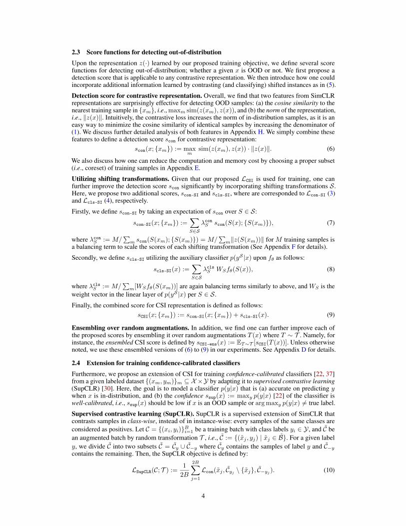
2.3 Score functions for detecting out-of-distribution

Upon the representation z(·) learned by our proposed training objective, we define several scorefunctions for detecting out-of-distribution; whether a given x is OOD or not. We first propose adetection score that is applicable to any contrastive representation. We then introduce how one couldincorporate additional information learned by contrasting (and classifying) shifted instances as in (5).

Detection score for contrastive representation. Overall, we find that two features from SimCLRrepresentations are surprisingly effective for detecting OOD samples: (a) the cosine similarity to thenearest training sample in {xm}, i.e., maxm sim(z(xm), z(x)), and (b) the norm of the representation,i.e., ‖z(x)‖. Intuitively, the contrastive loss increases the norm of in-distribution samples, as it is aneasy way to minimize the cosine similarity of identical samples by increasing the denominator of(1). We discuss further detailed analysis of both features in Appendix H. We simply combine thesefeatures to define a detection score scon for contrastive representation:

scon(x; {xm}) := maxm

sim(z(xm), z(x)) · ‖z(x)‖. (6)

We also discuss how one can reduce the computation and memory cost by choosing a proper subset(i.e., coreset) of training samples in Appendix E.

Utilizing shifting transformations. Given that our proposed LCSI is used for training, one canfurther improve the detection score scon significantly by incorporating shifting transformations S.Here, we propose two additional scores, scon-SI and scls-SI, where are corresponded to Lcon-SI (3)and Lcls-SI (4), respectively.

Firstly, we define scon-SI by taking an expectation of scon over S ∈ S:

scon-SI(x; {xm}) :=∑S∈S

λconS scon(S(x); {S(xm)}), (7)

where λconS :=M/∑m scon(S(xm); {S(xm)}) =M/

∑m‖z(S(xm))‖ for M training samples is

a balancing term to scale the scores of each shifting transformation (See Appendix F for details).

Secondly, we define scls-SI utilizing the auxiliary classifier p(yS |x) upon fθ as follows:

scls-SI(x) :=∑S∈S

λclsS WSfθ(S(x)), (8)

where λclsS :=M/∑m[WSfθ(S(xm))] are again balancing terms similarly to above, and WS is the

weight vector in the linear layer of p(yS |x) per S ∈ S.

Finally, the combined score for CSI representation is defined as follows:sCSI(x; {xm}) := scon-SI(x; {xm}) + scls-SI(x). (9)

Ensembling over random augmentations. In addition, we find one can further improve each ofthe proposed scores by ensembling it over random augmentations T (x) where T ∼ T . Namely, forinstance, the ensembled CSI score is defined by sCSI-ens(x) := ET∼T [sCSI(T (x))]. Unless otherwisenoted, we use these ensembled versions of (6) to (9) in our experiments. See Appendix D for details.

2.4 Extension for training confidence-calibrated classifiers

Furthermore, we propose an extension of CSI for training confidence-calibrated classifiers [22, 37]from a given labeled dataset {(xm, ym)}m ⊆ X ×Y by adapting it to supervised contrastive learning(SupCLR) [30]. Here, the goal is to model a classifier p(y|x) that is (a) accurate on predicting ywhen x is in-distribution, and (b) the confidence ssup(x) := maxy p(y|x) [22] of the classifier iswell-calibrated, i.e., ssup(x) should be low if x is an OOD sample or argmaxy p(y|x) 6= true label.

Supervised contrastive learning (SupCLR). SupCLR is a supervised extension of SimCLR thatcontrasts samples in class-wise, instead of in instance-wise: every samples of the same classes areconsidered as positives. Let C = {(xi, yi)}Bi=1 be a training batch with class labels yi ∈ Y , and C̃ bean augmented batch by random transformation T , i.e., C̃ := {(x̃j , yj) | x̃j ∈ B̃}. For a given labely, we divide C̃ into two subsets C̃ = C̃y ∪ C̃−y where C̃y contains the samples of label y and C̃−ycontains the remaining. Then, the SupCLR objective is defined by:

LSupCLR(C; T ) :=1

2B

2B∑j=1

Lcon(x̃j , C̃yj \ {x̃j}, C̃−yj ). (10)

4

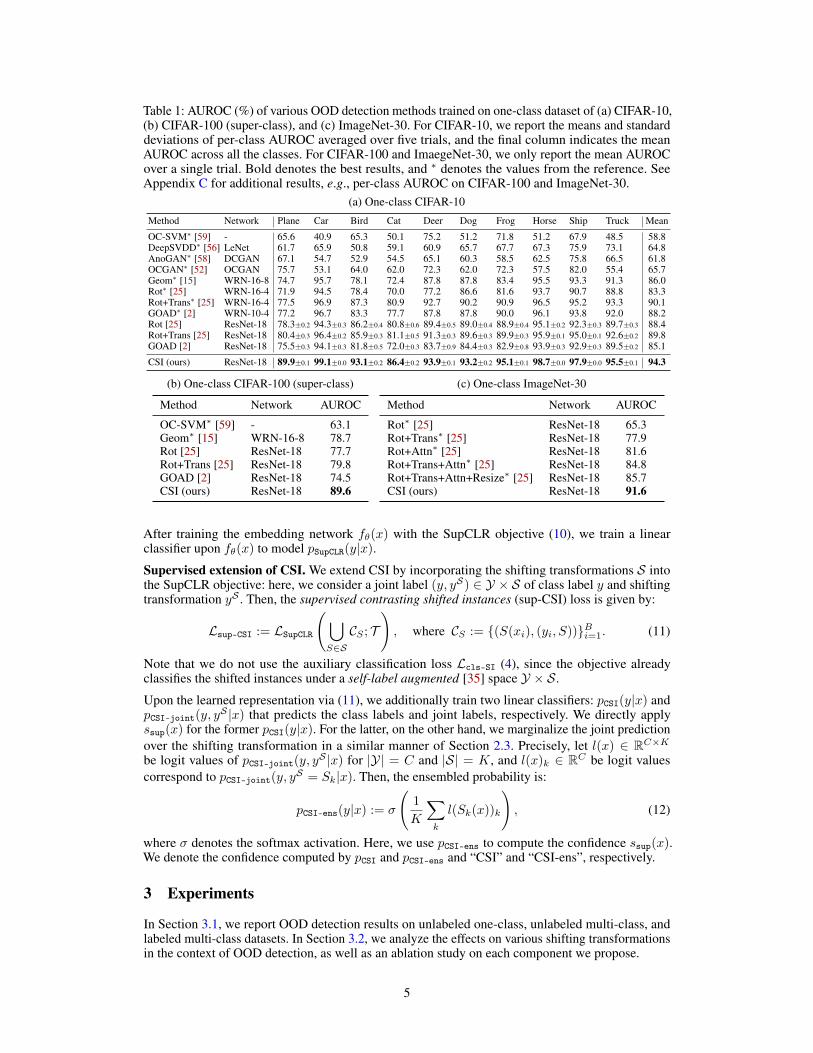
Table 1: AUROC (%) of various OOD detection methods trained on one-class dataset of (a) CIFAR-10,(b) CIFAR-100 (super-class), and (c) ImageNet-30. For CIFAR-10, we report the means and standarddeviations of per-class AUROC averaged over five trials, and the final column indicates the meanAUROC across all the classes. For CIFAR-100 and ImaegeNet-30, we only report the mean AUROCover a single trial. Bold denotes the best results, and ∗ denotes the values from the reference. SeeAppendix C for additional results, e.g., per-class AUROC on CIFAR-100 and ImageNet-30.

(a) One-class CIFAR-10

Method Network Plane Car Bird Cat Deer Dog Frog Horse Ship Truck Mean

OC-SVM∗ [59] - 65.6 40.9 65.3 50.1 75.2 51.2 71.8 51.2 67.9 48.5 58.8DeepSVDD∗ [56] LeNet 61.7 65.9 50.8 59.1 60.9 65.7 67.7 67.3 75.9 73.1 64.8AnoGAN∗ [58] DCGAN 67.1 54.7 52.9 54.5 65.1 60.3 58.5 62.5 75.8 66.5 61.8OCGAN∗ [52] OCGAN 75.7 53.1 64.0 62.0 72.3 62.0 72.3 57.5 82.0 55.4 65.7Geom∗ [15] WRN-16-8 74.7 95.7 78.1 72.4 87.8 87.8 83.4 95.5 93.3 91.3 86.0Rot∗ [25] WRN-16-4 71.9 94.5 78.4 70.0 77.2 86.6 81.6 93.7 90.7 88.8 83.3Rot+Trans∗ [25] WRN-16-4 77.5 96.9 87.3 80.9 92.7 90.2 90.9 96.5 95.2 93.3 90.1GOAD∗ [2] WRN-10-4 77.2 96.7 83.3 77.7 87.8 87.8 90.0 96.1 93.8 92.0 88.2Rot [25] ResNet-18 78.3±0.2 94.3±0.3 86.2±0.4 80.8±0.6 89.4±0.5 89.0±0.4 88.9±0.4 95.1±0.2 92.3±0.3 89.7±0.3 88.4Rot+Trans [25] ResNet-18 80.4±0.3 96.4±0.2 85.9±0.3 81.1±0.5 91.3±0.3 89.6±0.3 89.9±0.3 95.9±0.1 95.0±0.1 92.6±0.2 89.8GOAD [2] ResNet-18 75.5±0.3 94.1±0.3 81.8±0.5 72.0±0.3 83.7±0.9 84.4±0.3 82.9±0.8 93.9±0.3 92.9±0.3 89.5±0.2 85.1

CSI (ours) ResNet-18 89.9±0.1 99.1±0.0 93.1±0.2 86.4±0.2 93.9±0.1 93.2±0.2 95.1±0.1 98.7±0.0 97.9±0.0 95.5±0.1 94.3

(b) One-class CIFAR-100 (super-class)

Method Network AUROC

OC-SVM∗ [59] - 63.1Geom∗ [15] WRN-16-8 78.7Rot [25] ResNet-18 77.7Rot+Trans [25] ResNet-18 79.8GOAD [2] ResNet-18 74.5CSI (ours) ResNet-18 89.6

(c) One-class ImageNet-30

Method Network AUROC

Rot∗ [25] ResNet-18 65.3Rot+Trans∗ [25] ResNet-18 77.9Rot+Attn∗ [25] ResNet-18 81.6Rot+Trans+Attn∗ [25] ResNet-18 84.8Rot+Trans+Attn+Resize∗ [25] ResNet-18 85.7CSI (ours) ResNet-18 91.6

After training the embedding network fθ(x) with the SupCLR objective (10), we train a linearclassifier upon fθ(x) to model pSupCLR(y|x).Supervised extension of CSI. We extend CSI by incorporating the shifting transformations S intothe SupCLR objective: here, we consider a joint label (y, yS) ∈ Y × S of class label y and shiftingtransformation yS . Then, the supervised contrasting shifted instances (sup-CSI) loss is given by:

Lsup-CSI := LSupCLR

(⋃S∈SCS ; T

), where CS := {(S(xi), (yi, S))}Bi=1. (11)

Note that we do not use the auxiliary classification loss Lcls-SI (4), since the objective alreadyclassifies the shifted instances under a self-label augmented [35] space Y × S.

Upon the learned representation via (11), we additionally train two linear classifiers: pCSI(y|x) andpCSI-joint(y, y

S |x) that predicts the class labels and joint labels, respectively. We directly applyssup(x) for the former pCSI(y|x). For the latter, on the other hand, we marginalize the joint predictionover the shifting transformation in a similar manner of Section 2.3. Precisely, let l(x) ∈ RC×Kbe logit values of pCSI-joint(y, yS |x) for |Y| = C and |S| = K, and l(x)k ∈ RC be logit valuescorrespond to pCSI-joint(y, yS = Sk|x). Then, the ensembled probability is:

pCSI-ens(y|x) := σ

(1

K

∑k

l(Sk(x))k

), (12)

where σ denotes the softmax activation. Here, we use pCSI-ens to compute the confidence ssup(x).We denote the confidence computed by pCSI and pCSI-ens and “CSI” and “CSI-ens”, respectively.

3 Experiments

In Section 3.1, we report OOD detection results on unlabeled one-class, unlabeled multi-class, andlabeled multi-class datasets. In Section 3.2, we analyze the effects on various shifting transformationsin the context of OOD detection, as well as an ablation study on each component we propose.

5

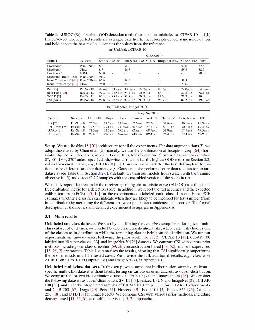
Table 2: AUROC (%) of various OOD detection methods trained on unlabeled (a) CIFAR-10 and (b)ImageNet-30. The reported results are averaged over five trials, subscripts denote standard deviation,and bold denote the best results. ∗ denotes the values from the reference.

(a) Unlabeled CIFAR-10

CIFAR10→Method Network SVHN LSUN ImageNet LSUN (FIX) ImageNet (FIX) CIFAR-100 Interp.

Likelihood∗ PixelCNN++ 8.3 - 64.2 - - 52.6 52.6Likelihood∗ Glow 8.3 - 66.3 - - 58.2 58.2Likelihood∗ EBM 63.0 - - - - - 70.0Likelihood Ratio∗ [55] PixelCNN++ 91.2 - - - - - -Input Complexity∗ [61] PixelCNN++ 92.9 - 58.9 - - 53.5 -Input Complexity∗ [61] Glow 95.0 - 71.6 - - 73.6 -

Rot [25] ResNet-18 97.6±0.2 89.2±0.7 90.5±0.3 77.7±0.3 83.2±0.1 79.0±0.1 64.0±0.3

Rot+Trans [25] ResNet-18 97.8±0.2 92.8±0.9 94.2±0.7 81.6±0.4 86.7±0.1 82.3±0.2 68.1±0.8

GOAD [2] ResNet-18 96.3±0.2 89.3±1.5 91.8±1.2 78.8±0.3 83.3±0.1 77.2±0.3 59.4±1.1

CSI (ours) ResNet-18 99.8±0.0 97.5±0.3 97.6±0.3 90.3±0.3 93.3±0.1 89.2±0.1 79.3±0.2

(b) Unlabeled ImageNet-30

ImageNet-30→Method Network CUB-200 Dogs Pets Flowers Food-101 Places-365 Caltech-256 DTD

Rot [25] ResNet-18 76.5±0.7 77.2±0.5 70.0±0.5 87.2±0.2 72.7±1.5 52.6±1.4 70.9±0.1 89.9±0.5

Rot+Trans [25] ResNet-18 74.5±0.5 77.8±1.1 70.0±0.8 86.3±0.3 71.6±1.4 53.1±1.7 70.0±0.2 89.4±0.6

GOAD [2] ResNet-18 71.5±1.4 74.3±1.6 65.5±1.3 82.8±1.4 68.7±0.7 51.0±1.1 67.4±0.8 87.5±0.8

CSI (ours) ResNet-18 90.5±0.1 97.1±0.1 85.2±0.2 94.7±0.4 89.2±0.3 78.3±0.3 87.1±0.1 96.9±0.1

Setup. We use ResNet-18 [20] architecture for all the experiments. For data augmentations T , weadopt those used by Chen et al. [5]: namely, we use the combination of Inception crop [64], hori-zontal flip, color jitter, and grayscale. For shifting transformations S, we use the random rotation0°, 90°, 180°, 270° unless specified otherwise, as rotation has the highest OOD-ness (see Section 2.2)values for natural images, e.g., CIFAR-10 [33]. However, we remark that the best shifting transforma-tion can be different for other datasets, e.g., Gaussian noise performs better than rotation for texturedatasets (see Table 6 in Section 3.2). By default, we train our models from scratch with the trainingobjective in (5) and detect OOD samples with the ensembled version of the score in (9).

We mainly report the area under the receiver operating characteristic curve (AUROC) as a threshold-free evaluation metric for a detection score. In addition, we report the test accuracy and the expectedcalibration error (ECE) [45, 19] for the experiments on labeled multi-class datasets. Here, ECEestimates whether a classifier can indicate when they are likely to be incorrect for test samples (fromin-distribution) by measuring the difference between prediction confidence and accuracy. The formaldescription of the metrics and detailed experimental setups are in Appendix A.

3.1 Main results

Unlabeled one-class datasets. We start by considering the one-class setup: here, for a given multi-class dataset of C classes, we conduct C one-class classification tasks, where each task chooses oneof the classes as in-distribution while the remaining classes being out-of-distribution. We run ourexperiments on three datasets, following the prior work [15, 25, 2]: CIFAR-10 [33], CIFAR-100labeled into 20 super-classes [33], and ImageNet-30 [25] datasets. We compare CSI with various priormethods including one-class classifier [59, 56], reconstruction-based [58, 52], and self-supervised[15, 25, 2] approaches. Table 1 summarizes the results, showing that CSI significantly outperformsthe prior methods in all the tested cases. We provide the full, additional results, e.g., class-wiseAUROC on CIFAR-100 (super-class) and ImageNet-30, in Appendix C.

Unlabeled multi-class datasets. In this setup, we assume that in-distribution samples are from aspecific multi-class dataset without labels, testing on various external datasets as out-of-distribution.We compare CSI on two in-distribution datasets: CIFAR-10 [33] and ImageNet-30 [25]. We considerthe following datasets as out-of-distribution: SVHN [48], resized LSUN and ImageNet [39], CIFAR-100 [33], and linearly-interpolated samples of CIFAR-10 (Interp.) [11] for CIFAR-10 experiments,and CUB-200 [67], Dogs [29], Pets [51], Flowers [49], Food-101 [3], Places-365 [75], Caltech-256 [18], and DTD [8] for ImageNet-30. We compare CSI with various prior methods, includingdensity-based [11, 55, 61] and self-supervised [15, 2] approaches.

6

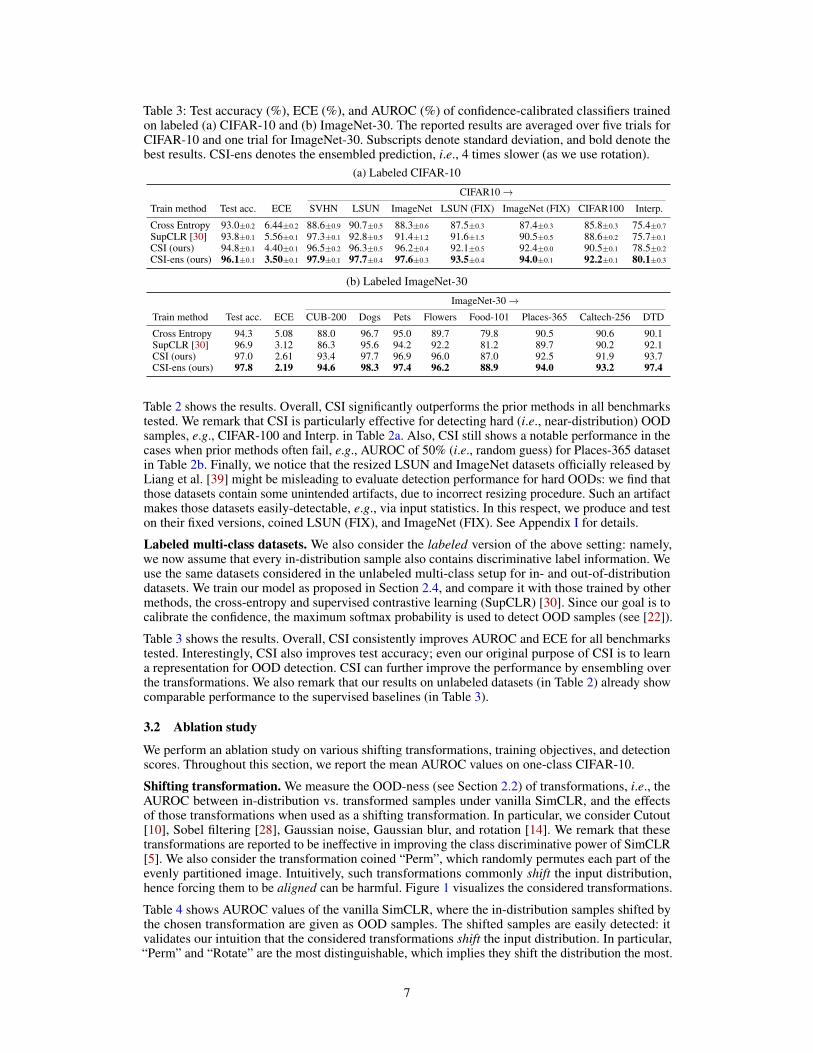
Table 3: Test accuracy (%), ECE (%), and AUROC (%) of confidence-calibrated classifiers trainedon labeled (a) CIFAR-10 and (b) ImageNet-30. The reported results are averaged over five trials forCIFAR-10 and one trial for ImageNet-30. Subscripts denote standard deviation, and bold denote thebest results. CSI-ens denotes the ensembled prediction, i.e., 4 times slower (as we use rotation).

(a) Labeled CIFAR-10

CIFAR10→Train method Test acc. ECE SVHN LSUN ImageNet LSUN (FIX) ImageNet (FIX) CIFAR100 Interp.

Cross Entropy 93.0±0.2 6.44±0.2 88.6±0.9 90.7±0.5 88.3±0.6 87.5±0.3 87.4±0.3 85.8±0.3 75.4±0.7

SupCLR [30] 93.8±0.1 5.56±0.1 97.3±0.1 92.8±0.5 91.4±1.2 91.6±1.5 90.5±0.5 88.6±0.2 75.7±0.1

CSI (ours) 94.8±0.1 4.40±0.1 96.5±0.2 96.3±0.5 96.2±0.4 92.1±0.5 92.4±0.0 90.5±0.1 78.5±0.2

CSI-ens (ours) 96.1±0.1 3.50±0.1 97.9±0.1 97.7±0.4 97.6±0.3 93.5±0.4 94.0±0.1 92.2±0.1 80.1±0.3

(b) Labeled ImageNet-30

ImageNet-30→Train method Test acc. ECE CUB-200 Dogs Pets Flowers Food-101 Places-365 Caltech-256 DTD

Cross Entropy 94.3 5.08 88.0 96.7 95.0 89.7 79.8 90.5 90.6 90.1SupCLR [30] 96.9 3.12 86.3 95.6 94.2 92.2 81.2 89.7 90.2 92.1CSI (ours) 97.0 2.61 93.4 97.7 96.9 96.0 87.0 92.5 91.9 93.7CSI-ens (ours) 97.8 2.19 94.6 98.3 97.4 96.2 88.9 94.0 93.2 97.4

Table 2 shows the results. Overall, CSI significantly outperforms the prior methods in all benchmarkstested. We remark that CSI is particularly effective for detecting hard (i.e., near-distribution) OODsamples, e.g., CIFAR-100 and Interp. in Table 2a. Also, CSI still shows a notable performance in thecases when prior methods often fail, e.g., AUROC of 50% (i.e., random guess) for Places-365 datasetin Table 2b. Finally, we notice that the resized LSUN and ImageNet datasets officially released byLiang et al. [39] might be misleading to evaluate detection performance for hard OODs: we find thatthose datasets contain some unintended artifacts, due to incorrect resizing procedure. Such an artifactmakes those datasets easily-detectable, e.g., via input statistics. In this respect, we produce and teston their fixed versions, coined LSUN (FIX), and ImageNet (FIX). See Appendix I for details.

Labeled multi-class datasets. We also consider the labeled version of the above setting: namely,we now assume that every in-distribution sample also contains discriminative label information. Weuse the same datasets considered in the unlabeled multi-class setup for in- and out-of-distributiondatasets. We train our model as proposed in Section 2.4, and compare it with those trained by othermethods, the cross-entropy and supervised contrastive learning (SupCLR) [30]. Since our goal is tocalibrate the confidence, the maximum softmax probability is used to detect OOD samples (see [22]).

Table 3 shows the results. Overall, CSI consistently improves AUROC and ECE for all benchmarkstested. Interestingly, CSI also improves test accuracy; even our original purpose of CSI is to learna representation for OOD detection. CSI can further improve the performance by ensembling overthe transformations. We also remark that our results on unlabeled datasets (in Table 2) already showcomparable performance to the supervised baselines (in Table 3).

3.2 Ablation study

We perform an ablation study on various shifting transformations, training objectives, and detectionscores. Throughout this section, we report the mean AUROC values on one-class CIFAR-10.

Shifting transformation. We measure the OOD-ness (see Section 2.2) of transformations, i.e., theAUROC between in-distribution vs. transformed samples under vanilla SimCLR, and the effectsof those transformations when used as a shifting transformation. In particular, we consider Cutout[10], Sobel filtering [28], Gaussian noise, Gaussian blur, and rotation [14]. We remark that thesetransformations are reported to be ineffective in improving the class discriminative power of SimCLR[5]. We also consider the transformation coined “Perm”, which randomly permutes each part of theevenly partitioned image. Intuitively, such transformations commonly shift the input distribution,hence forcing them to be aligned can be harmful. Figure 1 visualizes the considered transformations.

Table 4 shows AUROC values of the vanilla SimCLR, where the in-distribution samples shifted bythe chosen transformation are given as OOD samples. The shifted samples are easily detected: itvalidates our intuition that the considered transformations shift the input distribution. In particular,“Perm” and “Rotate” are the most distinguishable, which implies they shift the distribution the most.

7

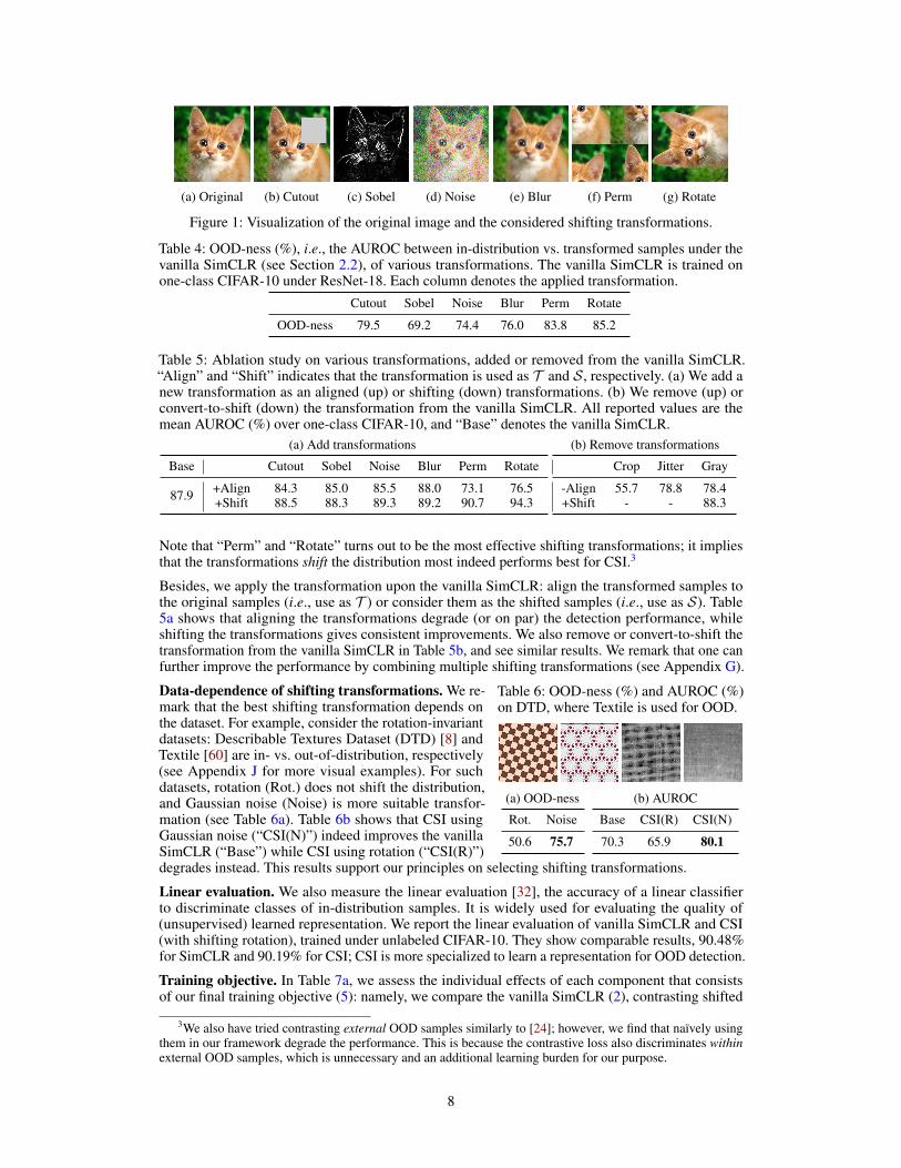
(a) Original (b) Cutout (c) Sobel (d) Noise (e) Blur (f) Perm (g) Rotate

Figure 1: Visualization of the original image and the considered shifting transformations.

Table 4: OOD-ness (%), i.e., the AUROC between in-distribution vs. transformed samples under thevanilla SimCLR (see Section 2.2), of various transformations. The vanilla SimCLR is trained onone-class CIFAR-10 under ResNet-18. Each column denotes the applied transformation.

Cutout Sobel Noise Blur Perm Rotate

OOD-ness 79.5 69.2 74.4 76.0 83.8 85.2

Table 5: Ablation study on various transformations, added or removed from the vanilla SimCLR.“Align” and “Shift” indicates that the transformation is used as T and S, respectively. (a) We add anew transformation as an aligned (up) or shifting (down) transformations. (b) We remove (up) orconvert-to-shift (down) the transformation from the vanilla SimCLR. All reported values are themean AUROC (%) over one-class CIFAR-10, and “Base” denotes the vanilla SimCLR.

(a) Add transformations

Base Cutout Sobel Noise Blur Perm Rotate

87.9 +Align 84.3 85.0 85.5 88.0 73.1 76.5+Shift 88.5 88.3 89.3 89.2 90.7 94.3

(b) Remove transformations

Crop Jitter Gray

-Align 55.7 78.8 78.4+Shift - - 88.3

Note that “Perm” and “Rotate” turns out to be the most effective shifting transformations; it impliesthat the transformations shift the distribution most indeed performs best for CSI.3

Besides, we apply the transformation upon the vanilla SimCLR: align the transformed samples tothe original samples (i.e., use as T ) or consider them as the shifted samples (i.e., use as S). Table5a shows that aligning the transformations degrade (or on par) the detection performance, whileshifting the transformations gives consistent improvements. We also remove or convert-to-shift thetransformation from the vanilla SimCLR in Table 5b, and see similar results. We remark that one canfurther improve the performance by combining multiple shifting transformations (see Appendix G).

Table 6: OOD-ness (%) and AUROC (%)on DTD, where Textile is used for OOD.

(a) OOD-ness

Rot. Noise

50.6 75.7

(b) AUROC

Base CSI(R) CSI(N)

70.3 65.9 80.1

Data-dependence of shifting transformations. We re-mark that the best shifting transformation depends onthe dataset. For example, consider the rotation-invariantdatasets: Describable Textures Dataset (DTD) [8] andTextile [60] are in- vs. out-of-distribution, respectively(see Appendix J for more visual examples). For suchdatasets, rotation (Rot.) does not shift the distribution,and Gaussian noise (Noise) is more suitable transfor-mation (see Table 6a). Table 6b shows that CSI usingGaussian noise (“CSI(N)”) indeed improves the vanillaSimCLR (“Base”) while CSI using rotation (“CSI(R)”)degrades instead. This results support our principles on selecting shifting transformations.

Linear evaluation. We also measure the linear evaluation [32], the accuracy of a linear classifierto discriminate classes of in-distribution samples. It is widely used for evaluating the quality of(unsupervised) learned representation. We report the linear evaluation of vanilla SimCLR and CSI(with shifting rotation), trained under unlabeled CIFAR-10. They show comparable results, 90.48%for SimCLR and 90.19% for CSI; CSI is more specialized to learn a representation for OOD detection.

Training objective. In Table 7a, we assess the individual effects of each component that consistsof our final training objective (5): namely, we compare the vanilla SimCLR (2), contrasting shifted

3We also have tried contrasting external OOD samples similarly to [24]; however, we find that naïvely usingthem in our framework degrade the performance. This is because the contrastive loss also discriminates withinexternal OOD samples, which is unnecessary and an additional learning burden for our purpose.

8

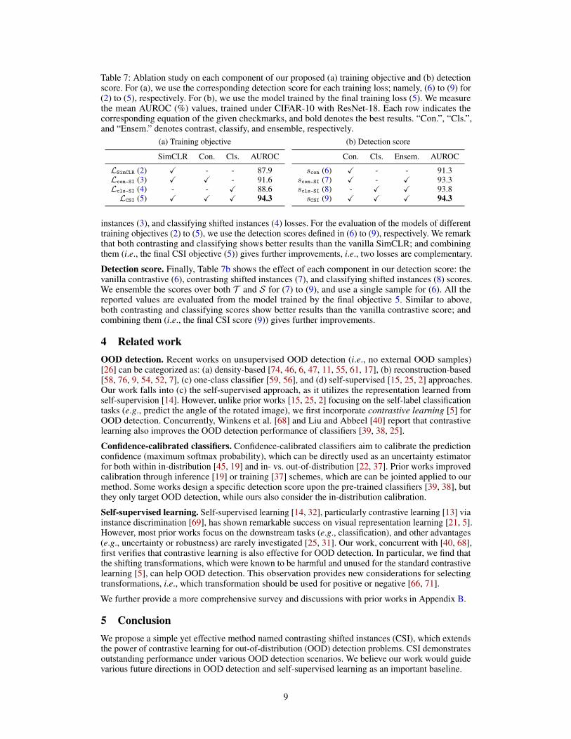
Table 7: Ablation study on each component of our proposed (a) training objective and (b) detectionscore. For (a), we use the corresponding detection score for each training loss; namely, (6) to (9) for(2) to (5), respectively. For (b), we use the model trained by the final training loss (5). We measurethe mean AUROC (%) values, trained under CIFAR-10 with ResNet-18. Each row indicates thecorresponding equation of the given checkmarks, and bold denotes the best results. “Con.”, “Cls.”,and “Ensem.” denotes contrast, classify, and ensemble, respectively.

(a) Training objective

SimCLR Con. Cls. AUROC

LSimCLR (2) X - - 87.9Lcon-SI (3) X X - 91.6Lcls-SI (4) - - X 88.6

LCSI (5) X X X 94.3

(b) Detection score

Con. Cls. Ensem. AUROC

scon (6) X - - 91.3scon-SI (7) X - X 93.3scls-SI (8) - X X 93.8

sCSI (9) X X X 94.3

instances (3), and classifying shifted instances (4) losses. For the evaluation of the models of differenttraining objectives (2) to (5), we use the detection scores defined in (6) to (9), respectively. We remarkthat both contrasting and classifying shows better results than the vanilla SimCLR; and combiningthem (i.e., the final CSI objective (5)) gives further improvements, i.e., two losses are complementary.

Detection score. Finally, Table 7b shows the effect of each component in our detection score: thevanilla contrastive (6), contrasting shifted instances (7), and classifying shifted instances (8) scores.We ensemble the scores over both T and S for (7) to (9), and use a single sample for (6). All thereported values are evaluated from the model trained by the final objective 5. Similar to above,both contrasting and classifying scores show better results than the vanilla contrastive score; andcombining them (i.e., the final CSI score (9)) gives further improvements.

4 Related workOOD detection. Recent works on unsupervised OOD detection (i.e., no external OOD samples)[26] can be categorized as: (a) density-based [74, 46, 6, 47, 11, 55, 61, 17], (b) reconstruction-based[58, 76, 9, 54, 52, 7], (c) one-class classifier [59, 56], and (d) self-supervised [15, 25, 2] approaches.Our work falls into (c) the self-supervised approach, as it utilizes the representation learned fromself-supervision [14]. However, unlike prior works [15, 25, 2] focusing on the self-label classificationtasks (e.g., predict the angle of the rotated image), we first incorporate contrastive learning [5] forOOD detection. Concurrently, Winkens et al. [68] and Liu and Abbeel [40] report that contrastivelearning also improves the OOD detection performance of classifiers [39, 38, 25].

Confidence-calibrated classifiers. Confidence-calibrated classifiers aim to calibrate the predictionconfidence (maximum softmax probability), which can be directly used as an uncertainty estimatorfor both within in-distribution [45, 19] and in- vs. out-of-distribution [22, 37]. Prior works improvedcalibration through inference [19] or training [37] schemes, which are can be jointed applied to ourmethod. Some works design a specific detection score upon the pre-trained classifiers [39, 38], butthey only target OOD detection, while ours also consider the in-distribution calibration.

Self-supervised learning. Self-supervised learning [14, 32], particularly contrastive learning [13] viainstance discrimination [69], has shown remarkable success on visual representation learning [21, 5].However, most prior works focus on the downstream tasks (e.g., classification), and other advantages(e.g., uncertainty or robustness) are rarely investigated [25, 31]. Our work, concurrent with [40, 68],first verifies that contrastive learning is also effective for OOD detection. In particular, we find thatthe shifting transformations, which were known to be harmful and unused for the standard contrastivelearning [5], can help OOD detection. This observation provides new considerations for selectingtransformations, i.e., which transformation should be used for positive or negative [66, 71].

We further provide a more comprehensive survey and discussions with prior works in Appendix B.

5 ConclusionWe propose a simple yet effective method named contrasting shifted instances (CSI), which extendsthe power of contrastive learning for out-of-distribution (OOD) detection problems. CSI demonstratesoutstanding performance under various OOD detection scenarios. We believe our work would guidevarious future directions in OOD detection and self-supervised learning as an important baseline.

9

Acknowledgements

This work was supported by Institute of Information & Communications Technology Planning& Evaluation (IITP) grant funded by the Korea government (MSIT) (No.2019-0-00075, ArtificialIntelligence Graduate School Program (KAIST) and No.2017-0-01779, A machine learning andstatistical inference framework for explainable artificial intelligence). We thank Sihyun Yu, ChaewonKim, Hyuntak Cha, Hyunwoo Kang, and Seunghyun Lee for helpful feedback and suggestions.

Broader Impact

This paper is focused on the subject of out-of-distribution (OOD) (or novelty, anomaly) detection,which is an essential ingredient for building safe and reliable intelligent systems [1]. We expect ourresults to have two consequences for academia and broader society.

Rethinking representation for OOD detection. In this paper, we demonstrate that the representationfor classification (or other related tasks, measured by linear evaluation [32]) can be different from therepresentation for OOD detection. In particular, we verify that the “hard” augmentations, thought to beharmful for contrastive representation learning [5], can be helpful for OOD detection. Our observationraises new questions for both representation learning and OOD detection: (a) representation learningresearches should also report the OOD detection results as an evaluation metric, (b) OOD detectionresearches should more investigate the specialized representation.

Towards reliable intelligent system. The intelligent system should be robust to the potential dangersof uncertain environments (e.g., financial crisis [65]) or malicious adversaries (e.g., cybersecurity[34]). Detecting outliers is also related to human safety (e.g., medical diagnosis [4] or autonomousdriving [12]), and has a broad range of industrial applications (e.g., manufacturing inspection [42]).However, the system can be stuck into confirmation bias, i.e., ignore new information with a myopicperspective. We hope the system to balance the exploration and exploitation of the knowledge.

References[1] D. Amodei, C. Olah, J. Steinhardt, P. Christiano, J. Schulman, and D. Mané. Concrete problems

in ai safety. arXiv preprint arXiv:1606.06565, 2016.

[2] L. Bergman and Y. Hoshen. Classification-based anomaly detection for general data. InInternational Conference on Learning Representations, 2020.

[3] L. Bossard, M. Guillaumin, and L. Van Gool. Food-101–mining discriminative componentswith random forests. In European Conference on Computer Vision, 2014.

[4] R. Caruana, Y. Lou, J. Gehrke, P. Koch, M. Sturm, and N. Elhadad. Intelligible models forhealthcare: Predicting pneumonia risk and hospital 30-day readmission. In ACM SIGKDDInternational Conference on Knowledge Discovery and Data Mining, 2015.

[5] T. Chen, S. Kornblith, M. Norouzi, and G. Hinton. A simple framework for contrastive learningof visual representations. In International Conference on Machine Learning, 2020.

[6] H. Choi, E. Jang, and A. A. Alemi. Waic, but why? generative ensembles for robust anomalydetection. arXiv preprint arXiv:1810.01392, 2018.

[7] S. Choi and S.-Y. Chung. Novelty detection via blurring. In International Conference onLearning Representations, 2020.

[8] M. Cimpoi, S. Maji, I. Kokkinos, S. Mohamed, and A. Vedaldi. Describing textures in the wild.In IEEE Conference on Computer Vision and Pattern Recognition, 2014.

[9] L. Deecke, R. Vandermeulen, L. Ruff, S. Mandt, and M. Kloft. Image anomaly detection withgenerative adversarial networks. In Joint European Conference on Machine Learning andKnowledge Discovery in Databases, 2018.

[10] T. DeVries and G. W. Taylor. Improved regularization of convolutional neural networks withcutout. arXiv preprint arXiv:1708.04552, 2017.

10

[11] Y. Du and I. Mordatch. Implicit generation and modeling with energy based models. InAdvances in Neural Information Processing Systems, 2019.

[12] K. Eykholt, I. Evtimov, E. Fernandes, B. Li, A. Rahmati, C. Xiao, A. Prakash, T. Kohno,and D. Song. Robust physical-world attacks on deep learning visual classification. In IEEEConference on Computer Vision and Pattern Recognition, 2018.

[13] W. Falcon and K. Cho. A framework for contrastive self-supervised learning and designing anew approach. arXiv preprint arXiv:2009.00104, 2020.

[14] S. Gidaris, P. Singh, and N. Komodakis. Unsupervised representation learning by predictingimage rotations. In International Conference on Learning Representations, 2018.

[15] I. Golan and R. El-Yaniv. Deep anomaly detection using geometric transformations. In Advancesin Neural Information Processing Systems, 2018.

[16] P. Goyal, P. Dollár, R. Girshick, P. Noordhuis, L. Wesolowski, A. Kyrola, A. Tulloch, Y. Jia,and K. He. Accurate, large minibatch sgd: Training imagenet in 1 hour. arXiv preprintarXiv:1706.02677, 2017.

[17] W. Grathwohl, K.-C. Wang, J.-H. Jacobsen, D. Duvenaud, M. Norouzi, and K. Swersky. Yourclassifier is secretly an energy based model and you should treat it like one. In InternationalConference on Learning Representations, 2020.

[18] G. Griffin, A. Holub, and P. Perona. Caltech-256 object category dataset, 2007.

[19] C. Guo, G. Pleiss, Y. Sun, and K. Q. Weinberger. On calibration of modern neural networks. InInternational Conference on Machine Learning, 2017.

[20] K. He, X. Zhang, S. Ren, and J. Sun. Deep residual learning for image recognition. In IEEEConference on Computer Vision and Pattern Recognition, 2016.

[21] K. He, H. Fan, Y. Wu, S. Xie, and R. Girshick. Momentum contrast for unsupervised visualrepresentation learning. In IEEE Conference on Computer Vision and Pattern Recognition,2020.

[22] D. Hendrycks and K. Gimpel. A baseline for detecting misclassified and out-of-distributionexamples in neural networks. In International Conference on Learning Representations, 2017.

[23] D. Hendrycks, K. Lee, and M. Mazeika. Using pre-training can improve model robustness anduncertainty. In International Conference on Machine Learning, 2019.

[24] D. Hendrycks, M. Mazeika, and T. Dietterich. Deep anomaly detection with outlier exposure.In International Conference on Learning Representations, 2019.

[25] D. Hendrycks, M. Mazeika, S. Kadavath, and D. Song. Using self-supervised learning canimprove model robustness and uncertainty. In Advances in Neural Information ProcessingSystems, 2019.

[26] V. Hodge and J. Austin. A survey of outlier detection methodologies. Artificial intelligencereview, 2004.

[27] S. Ioffe and C. Szegedy. Batch normalization: Accelerating deep network training by reducinginternal covariate shift. International Conference on Machine Learning, 2015.

[28] N. Kanopoulos, N. Vasanthavada, and R. L. Baker. Design of an image edge detection filterusing the sobel operator. IEEE Journal of solid-state circuits, 1988.

[29] A. Khosla, N. Jayadevaprakash, B. Yao, and L. Fei-Fei. Novel dataset for fine-grained imagecategorization. In IEEE Conference on Computer Vision and Pattern Recognition, ColoradoSprings, CO, June 2011.

[30] P. Khosla, P. Teterwak, C. Wang, A. Sarna, Y. Tian, P. Isola, A. Maschinot, C. Liu, andD. Krishnan. Supervised contrastive learning. In Advances in Neural Information ProcessingSystems, 2020.

11

[31] M. Kim, J. Tack, and S. J. Hwang. Adversarial self-supervised contrastive learning. In Advancesin Neural Information Processing Systems, 2020.

[32] A. Kolesnikov, X. Zhai, and L. Beyer. Revisiting self-supervised visual representation learning.In IEEE Conference on Computer Vision and Pattern Recognition, 2019.

[33] A. Krizhevsky et al. Learning multiple layers of features from tiny images, 2009.

[34] C. Kruegel and G. Vigna. Anomaly detection of web-based attacks. In Proceedings of the 10thACM conference on Computer and communications security, 2003.

[35] H. Lee, S. J. Hwang, and J. Shin. Self-supervised label augmentation via input transformations.In International Conference on Machine Learning, 2020.

[36] K. Lee, C. Hwang, K. S. Park, and J. Shin. Confident multiple choice learning. In InternationalConference on Machine Learning, 2017.

[37] K. Lee, H. Lee, K. Lee, and J. Shin. Training confidence-calibrated classifiers for detectingout-of-distribution samples. In International Conference on Learning Representations, 2018.

[38] K. Lee, K. Lee, H. Lee, and J. Shin. A simple unified framework for detecting out-of-distributionsamples and adversarial attacks. In Advances in Neural Information Processing Systems, 2018.

[39] S. Liang, Y. Li, and R. Srikant. Enhancing the reliability of out-of-distribution image detectionin neural networks. In International Conference on Learning Representations, 2018.

[40] H. Liu and P. Abbeel. Hybrid discriminative-generative training via contrastive learning. arXivpreprint arXiv:2007.09070, 2020.

[41] I. Loshchilov and F. Hutter. Sgdr: Stochastic gradient descent with warm restarts. arXiv preprintarXiv:1608.03983, 2016.

[42] D. Lucke, C. Constantinescu, and E. Westkämper. Smart factory-a step towards the nextgeneration of manufacturing. Manufacturing Systems and Technologies for the New Frontier,page 115, 2008.

[43] L. v. d. Maaten and G. Hinton. Visualizing data using t-sne. Journal of machine learningresearch, 2008.

[44] J. MacQueen et al. Some methods for classification and analysis of multivariate observations,1967.

[45] M. P. Naeini, G. Cooper, and M. Hauskrecht. Obtaining well calibrated probabilities usingbayesian binning. In AAAI Conference on Artificial Intelligence, 2015.

[46] E. Nalisnick, A. Matsukawa, Y. W. Teh, D. Gorur, and B. Lakshminarayanan. Do deep generativemodels know what they don’t know? In International Conference on Learning Representations,2019.

[47] E. Nalisnick, A. Matsukawa, Y. W. Teh, and B. Lakshminarayanan. Detecting out-of-distributioninputs to deep generative models using a test for typicality. arXiv preprint arXiv:1906.02994,2019.

[48] Y. Netzer, T. Wang, A. Coates, A. Bissacco, B. Wu, and A. Y. Ng. Reading digits in naturalimages with unsupervised feature learning. In Advances in Neural Information ProcessingSystems Workshop on Deep Learning and Unsupervised Feature Learning, 2011.

[49] M.-E. Nilsback and A. Zisserman. A visual vocabulary for flower classification. In IEEEConference on Computer Vision and Pattern Recognition, 2006.

[50] A. v. d. Oord, Y. Li, and O. Vinyals. Representation learning with contrastive predictive coding.arXiv preprint arXiv:1807.03748, 2018.

[51] O. M. Parkhi, A. Vedaldi, A. Zisserman, and C. Jawahar. Cats and dogs. In IEEE Conferenceon Computer Vision and Pattern Recognition, 2012.

12

[52] P. Perera, R. Nallapati, and B. Xiang. Ocgan: One-class novelty detection using gans withconstrained latent representations. In IEEE Conference on Computer Vision and PatternRecognition, 2019.

[53] C. Phua, V. Lee, K. Smith, and R. Gayler. A comprehensive survey of data mining-based frauddetection research. arXiv preprint arXiv:1009.6119, 2010.

[54] S. Pidhorskyi, R. Almohsen, and G. Doretto. Generative probabilistic novelty detection withadversarial autoencoders. In Advances in Neural Information Processing Systems, 2018.

[55] J. Ren, P. J. Liu, E. Fertig, J. Snoek, R. Poplin, M. Depristo, J. Dillon, and B. Lakshminarayanan.Likelihood ratios for out-of-distribution detection. In Advances in Neural Information Process-ing Systems, 2019.

[56] L. Ruff, R. Vandermeulen, N. Goernitz, L. Deecke, S. A. Siddiqui, A. Binder, E. Müller, andM. Kloft. Deep one-class classification. In International Conference on Machine Learning,2018.

[57] L. Ruff, R. A. Vandermeulen, N. Görnitz, A. Binder, E. Müller, K.-R. Müller, and M. Kloft. Deepsemi-supervised anomaly detection. In International Conference on Learning Representations,2020.

[58] T. Schlegl, P. Seeböck, S. M. Waldstein, U. Schmidt-Erfurth, and G. Langs. Unsupervisedanomaly detection with generative adversarial networks to guide marker discovery. In Interna-tional conference on information processing in medical imaging, 2017.

[59] B. Schölkopf, R. C. Williamson, A. J. Smola, J. Shawe-Taylor, and J. C. Platt. Support vectormethod for novelty detection. In Advances in Neural Information Processing Systems, 2000.

[60] H. Schulz-Mirbach. Tilda-ein referenzdatensatz zur evaluierung von sichtprüfungsverfahren fürtextiloberflächen. Interner Bericht, 1996. URL https://lmb.informatik.uni-freiburg.de/resources/datasets/tilda.en.html.

[61] J. Serrà, D. Álvarez, V. Gómez, O. Slizovskaia, J. F. Núñez, and J. Luque. Input complexityand out-of-distribution detection with likelihood-based generative models. In InternationalConference on Learning Representations, 2020.

[62] Severstal. Severstal: Steel defect detection, 2019. URL https://www.kaggle.com/c/severstal-steel-defect-detection.

[63] A. Srinivas, M. Laskin, and P. Abbeel. Curl: Contrastive unsupervised representations forreinforcement learning. In International Conference on Machine Learning, 2020.

[64] C. Szegedy, W. Liu, Y. Jia, P. Sermanet, S. Reed, D. Anguelov, D. Erhan, V. Vanhoucke, andA. Rabinovich. Going deeper with convolutions. In IEEE Conference on Computer Vision andPattern Recognition, pages 1–9, 2015.

[65] J. B. Taylor and J. C. Williams. A black swan in the money market. American EconomicJournal: Macroeconomics, 2009.

[66] Y. Tian, C. Sun, B. Poole, D. Krishnan, C. Schmid, and P. Isola. What makes for good views forcontrastive learning. In Advances in Neural Information Processing Systems, 2020.

[67] C. Wah, S. Branson, P. Welinder, P. Perona, and S. Belongie. The Caltech-UCSD Birds-200-2011Dataset. Technical Report CNS-TR-2011-001, California Institute of Technology, 2011.

[68] J. Winkens, R. Bunel, A. G. Roy, R. Stanforth, V. Natarajan, J. R. Ledsam, P. MacWilliams,P. Kohli, A. Karthikesalingam, and S. Kohl. Contrastive training for improved out-of-distributiondetection. arXiv preprint arXiv:2007.05566, 2020.

[69] Z. Wu, Y. Xiong, S. X. Yu, and D. Lin. Unsupervised feature learning via non-parametricinstance discrimination. In IEEE Conference on Computer Vision and Pattern Recognition,2018.

13

[70] G.-S. Xia, X. Bai, J. Ding, Z. Zhu, S. Belongie, J. Luo, M. Datcu, M. Pelillo, and L. Zhang. Dota:A large-scale dataset for object detection in aerial images. In IEEE Conference on ComputerVision and Pattern Recognition, 2018.

[71] T. Xiao, X. Wang, A. A. Efros, and T. Darrell. What should not be contrastive in contrastivelearning. arXiv preprint arXiv:2008.05659, 2020.

[72] Y. You, I. Gitman, and B. Ginsburg. Large batch training of convolutional networks. arXivpreprint arXiv:1708.03888, 2017.

[73] S. Yun, J. Park, K. Lee, and J. Shin. Regularizing class-wise predictions via self-knowledgedistillation. In IEEE Conference on Computer Vision and Pattern Recognition, 2020.

[74] S. Zhai, Y. Cheng, W. Lu, and Z. Zhang. Deep structured energy based models for anomalydetection. In International Conference on Machine Learning, 2016.

[75] B. Zhou, A. Lapedriza, A. Khosla, A. Oliva, and A. Torralba. Places: A 10 million imagedatabase for scene recognition. IEEE Transactions on Pattern Analysis and Machine Intelligence,2017.

[76] B. Zong, Q. Song, M. R. Min, W. Cheng, C. Lumezanu, D. Cho, and H. Chen. Deep autoencod-ing gaussian mixture model for unsupervised anomaly detection. In International Conferenceon Learning Representations, 2018.

14