arX

iv:h

ep-t

h/04

0525

9v2

15

Mar

200

5

Preprint typeset in JHEP style - HYPER VERSION LPTENS-04/27

RI-05-04

hep-th/0405259

D-branes in N=2 Liouville theory and its mirror

Dan Israel1, Ari Pakman2,3 and Jan Troost1

1 Laboratoire de Physique Theorique de l’Ecole Normale Superieure∗

24, Rue Lhomond, 75231 Paris Cedex 05, France

2 Racah Institute of Physics, The Hebrew University

Jerusalem 91904, Israel

3 Erwin Schrodinger International Institute for Mathematical Physics

Boltzmanngasse 9, A-1090 Vienna, Austria

E-mail: israel@lpt.ens.fr, pakman@phys.huji.ac.il, troost@lpt.ens.fr

Abstract: We study D-branes in the mirror pair N = 2 Liouville/supersymmetric

SL(2,R)/U(1) coset superconformal field theories. After revisiting the duality between

the two models, we build D0, D1 and D2 branes, on the basis of the boundary state con-

struction for the H+3 conformal field theory. We also construct D0-branes in an orbifold

that rotates the angular direction of the cigar. We show how the poles of correlators associ-

ated to localized states and bulk interactions naturally decouple in the one-point functions

of localized and extended branes. We stress the role played in the analysis of D-brane

spectra by primaries in SL(2,R)/U(1) which are descendents of the parent theory.

∗Unite mixte du CNRS et de l’Ecole Normale Superieure, UMR 8549.

Contents

1. Introduction 2

2. The bulk 2

2.1 The bulk spectrum of the supersymmetric coset 3

2.2 Towards the duality with N = 2 Liouville: a bosonic ancestor 4

2.3 The supersymmetric case 7

2.4 Bulk versus localized poles and self-duality 9

2.5 The conformal bootstrap approach 10

3. The boundary 12

4. D0-branes 13

4.1 One-point function for the localized branes 13

4.2 Cardy computation for the D0-branes 15

5. D0 branes in a Zp orbifold 20

6. D1 branes 24

7. D2-branes 26

7.1 D1-like contribution 26

7.2 D0-like contribution 27

8. Conclusions 29

A. Computing N=2, c>3 characters 30

B. Changing basis in SL(2,R) 37

C. Cardy condition for D0 branes in R/NS sectors 39

D. Embedding N = 2 into SL(2,R) 41

E. Conventions 42

– 1 –

1. Introduction

We have learned that it is very useful to study non-perturbative objects in string theory, es-

pecially when they are related to an implementation of holography. This study has proved

instrumental both for understanding gauge theory physics, and for getting to grips with

aspects of quantum gravity. In this paper, we will concentrate on constructing boundary

conformal field theories for theories with N = 2 supersymmetry and central charge c > 3.

These boundary conformal field theories are arguably the most important missing ingredi-

ent in the construction of D-branes in non-compact curved string backgrounds with bulk

supersymmetry.

The models we will study in detail are the N = 2 Liouville theory [1, 2], and the

SL(2,R)/U(1) super-coset [3] theory. These two theories are known to be dual [4, 5](see

also [6, 7]), and are mapped to each other by mirror symmetry.

Constructing D-branes in these superconformal field theories will not only increase

our knowledge of D-branes in non-minimal N = 2 superconformal field theories (see also

[10, 11, 12]), but it will also enable us to study holographic dualities in closer detail.

There are two conjectured instances of holography where these D-branes are expected to

be relevant. The N = 2 Liouville/SL(2,R)/U(1) background is is related to a conjectured

calculable version of holography [5] which involves a bulk closed superstring background [8]

dual to a non-gravitational non-local Little String Theory [9]. Note for instance that D1-

branes stretching between NS5-branes (which can be interpreted as the W-bosons of the

Little String Theory) can be constructed using these boundary conformal field theories.

Another natural area where the D-branes built in this model are relevant is the study

of matrix models for two-dimensional non-critical superstrings [11] and Type 0 strings in

a 2D black hole. For the latter case, it was conjectured in [13], following the ideas of [14],

that the decoupled theory of N → ∞ D0 branes of ZZ type in N = 2 Liouville, leads to a

version of the matrix model of [15] with the matrix eigenvalues filling symmetrically both

sides of the inverted harmonic oscillator potential. This matrix model would be dual to

2D Type 0A string theory in the supersymmetric 2D black hole background.

Our paper is structured as follows. We first review in section 2 the bulk theories, and

the duality between N = 2 Liouville theory and the supersymmetric coset. In section 3 we

go on to discuss how to relate H+3 (i.e. Euclidean AdS3) boundary conformal field theories

to the N = 2 theories under consideration. In the following sections, we then explicitly

construct and study D0-, D1- and D2-branes. We pause in section 5 to explain how to

extend our result to an angular orbifold of the cigar. In the appendices, we collect several

important remarks. One concerns the fact that the SL(2,R)/U(1) super-coset characters

are equal to the characters of the N = 2, c > 3 Virasoro algebra. Another treats the Fourier

transformation of the one-point functions, while a third appendix analyzes the SL(2,R)

symmetry of general N = 2 c > 3 conformal field theories.

2. The bulk

In this section we will study aspects of the bulk theory in which the D-branes studied in this

– 2 –

paper will be embedded. We give original points of view on some of the topics treated in the

literature. We first discuss the spectrum of the supersymmetric SL(2,R)/U(1) conformal

field theory for concreteness. We then study the nature of the duality between the susy

coset and N = 2 Liouville (as well as its bosonic counterpart). We next review the pole

structure of the bulk correlators and comment upon the pole structure of the one-point

functions. We finish by suggesting that from the perspective of recent developments in

non-rational conformal field theories, the duality of the two theories is a case of dynamics

being completely determined by chiral symmetries.

2.1 The bulk spectrum of the supersymmetric coset

We consider a bulk theory with N = 2 supersymmetry, namely the axial SL(2,R)/U(1)

super-coset conformal field theory [3]. We review the algebraic details of this N = 2 algebra

in Appendix A. The central charge of the conformal field theory is

c = 3 +6

k, (2.1)

where k is the level of the parent (total) SL(2,R) current algebra. The primaries Φjm,m in

the bulk, coming from SL(2,R) primaries with spin j, can belong either to the NS or R

sector of the N = 2 algebra. They have conformal dimensions and N = 2 R-charges [13, 8]

∆j,w,n = −j(j − 1)

k+m2

k+

(δR±)2

8Qj,w,n =

2m

k+δR±

2,

∆j,w,n = −j(j − 1)

k+m2

k+

(δR±)2

8Qj,w,n = −2m

k− δR

±

2, (2.2)

where

m =n+ kw

2m = −n− kw

2, (2.3)

with n,w ∈ Z. The constant δR± is zero in the NS sector and ±1 in the R sector. The

Ramond primaries appear always in pairs due to the double degeneracy of the Ramond

vacuum. The numbers m, m are the eigenvalues of the left and right elliptic generators of

the SL(2,R) Lie algebra. Notice that the conformal dimension ∆j,w,n is invariant under

j → −j + 1. The two corresponding primaries are related through

Φ−j+1m,m = RNS/R±

(−j + 1,m, m) Φjm,m ,

=1

RNS/R±(j,m, m)Φj

m,m , (2.4)

where the reflection coefficients RNS/R±

(j,m, m) are given by [13]

RNS(j,m, m) = ν1−2j Γ(−2j + 1)Γ(1 + 1−2jk )

Γ(2j − 1)Γ(1 − 1−2jk )

Γ(j +m)Γ(j − m)

Γ(−j + 1 +m)Γ(−j + 1 − m), (2.5)

RR±

(j,m, m) = ν1−2j Γ(−2j + 1)Γ(1 + 1−2jk )

Γ(2j − 1)Γ(1 − 1−2jk )

Γ(j +m± 12 )Γ(j − m∓ 1

2)

Γ(−j + 1 +m± 12 )Γ(−j + 1 − m∓ 1

2),

(2.6)

– 3 –

for primaries of the NS and R sectors, respectively.

The two-dimensional geometry of the axial coset theory is a cigar [16, 17], or Euclidean

2D black hole [18, 19] . It has an asymptotic radius equal to√kα′, and the quantum number

n is interpreted in the axial SL(2,R)/U(1) coset as the momentum around the compact

circle at infinity. The number w denotes the winding number of the closed string states [20],

but can be viewed also as the spectral flow parameter of the affine SL(2,R) algebra [21, 22].

The spectrum of the super-coset includes both continuous representations with j =12 + iP (and P ∈ R

+0 ), and discrete lowest-weight representations D+

j [20] with values of

j ∈ R satisfying

1

2< j <

k + 1

2, (2.7)

and

j + r = m, j + r = m , (2.8)

where r, r are integers (half-integers) for the Neveu-Schwarz (Ramond) sector. The bound

for j (2.7) is stricter than the unitarity bound on the coset representations [23] as well as

than the bound corresponding to normalizable operators [22]. The improved bound has

been shown to apply in all physical settings [5, 22, 24, 25, 26, 8]. Although coset primaries

for discrete representations appear for all values of r, r, only those with r, r ≥ 0 correspond

to coset primaries inherited from SL(2,R) primaries, and only for them expressions (2.2)

hold. The coset primaries with r, r < 0 arise from descendants of SL(2,R) discrete lowest-

weight representations D+j , but they can be interpreted as primaries coming from discrete

highest-weight representations D−k+22

−jwith spin k+2

2 − j. We discuss the details of the

r, r < 0 primaries in this section, in section 4.1 and in Appendix A.1

The spectrum of primaries that we have reviewed above follows from studying the

representation of the affine SL(2,R) algebra and from the analysis of the modular invariant

partition function of the model [24, 26, 8]. The reflection coefficients (2.5)-(2.6) are related

to the dynamics of the theory, i.e. the correlation functions, which we consider now.

2.2 Towards the duality with N = 2 Liouville: a bosonic ancestor

Before discussing the duality between the susy coset SL(2,R)/U(1) and N = 2 Liouville,

we will look at its bosonic counterpart. The correlators of the bosonic SL(2,R)/U(1)

theory can be obtained by free field computations in SL(2,R). For this one can use the

Wakimoto free field representation of the algebra2

j+ = β

j3 = −βγ − 1

Q∂φ

j− = βγ2 +2

Qγ∂φ+ k∂γ (2.9)

1Note that when we take into account all primaries including those with r, r′ < 0, there is no need to

consider both D+ and D− representations, the D+ representations being enough to cover all the spectrum.2We will take the SL(2,R) level k+ 2, which is more convenient in order to move to the susy case later.

We take α′ = 2.

– 4 –

where

Q =

√2

k∆(β, γ) = (1, 0)

β(z)γ(w) ∼ 1

z − wφ(w)φ(z) ∼ − log(z − w) (2.10)

and the energy momentum tensor of the theory is:

T = β∂γ − 1

2(∂φ)2 − Q

2∂2φ , (2.11)

with the central charge given by (2.1). The SL(2,R) vertex operators are represented by

Φjm,m = γj+m−1γj+m−1e(j−1)Qφ . (2.12)

Correlators were computed in this formalism first in [27], by using the screening charge3

L1 = µ1ββe−Qφ . (2.13)

The two-point function is

〈Φjm,mΦj′

m,m〉 = |z12|−4∆jδn+n′δw+w′

(δ(j + j′ − 1) +RNS(j,m, m)δ(j − j′)

)(2.14)

where RNS(j,m, m) is given in (2.5). Similar free field computations can be performed

using a dual screening charge [28, 29, 30]

L2 = µ2(ββ)ke−2Q

φ , (2.15)

and the correlators agree under the identification [29]

πµ2Γ(k)

Γ(1 − k)=

(πµ1

Γ(k−1)

Γ(1 − k−1)

)k

. (2.16)

The vertex operators (2.12) correspond to the SL(2,R) theory. To obtain the primaries

of the coset one multiplies them by the exponential of a free boson, which represents the

gauged coordinate. But the nontrivial part of any correlator computed is the same in

SL(2,R) or SL(2,R)/U(1) since both interaction terms L1 and L2 commute with the

gauged current j3.

The free field formalism actually allows to compute (2.14) by inserting both L1 and

L2, and only for those values of j where the anomalous momentum conservation for φ is

satisfied as

2(j − 1)Q− n1Q− n22

Q= −Q , (2.17)

3Whenever we say screening charge we imply the integrated form∫d2z L.

– 5 –

where n1, n2 = 0, 1, . . . are the number of insertions of L1 and L2, respectively4. The

results are then analytically continued to arbitrary j.

In the limit φ→ ∞ the potential drops exponentially and the theory becomes weakly

coupled. In the cigar geometry, the dilaton becomes linear in φ, which has the interpretation

of the radial coordinate away from the tip. Following [15], it is easy to see that the relation

between L1 and L2 is that of a strong-weak coupling duality. For k → ∞, L2 is supported

in the strong coupling region (φ→ −∞) and L1 has support in the weak coupling region.

This is consistent with the fact the L1 screening can be obtained from the geometry of the

parent theory, by parameterizing AdS3 with Poincare coordinates, and the geometry of the

cigar becomes weakly curved at k → ∞ since the radius tends to infinity. The relation is

inverted at the opposite limit k → 0. Notice that all this is consistent with the fact that

µ1 and µ2 are interchanged under k ↔ k−1 as follows from (2.16).

It was first observed in [4] that correlators computed in the bosonic SL(2,R)/U(1)

model coincide with those of the sine-Liouville model, whose fields are a compact boson

X at the radius R =√

2(k + 2) of the cigar, and a non-compact one φ with background

charge. The stress tensor of the theory is

T = −1

2(∂X)2 − 1

2(∂φ)2 − Q

2∂2φ , (2.18)

and the central charge is5 c = 2 + 6k . The SL(2,R)/U(1) primaries are mapped to the

following primaries of sine-Liouville:

Φjm,m = e

im√

2k+2

XL+im√

2k+2

XRe(j−1)Qφ . (2.19)

The correlation functions are computed in the Coulomb formalism by using the screening

charges

L±sl = µsle

±i√

k+22

(XL−XR)e− 1

Qρ, (2.20)

which are primaries of ±1 winding in the compact boson. The relevant computations can

be found in [31] for the two-point functions and in [32] for some three point functions.6

Using L±sl as screening charges, the anomalous momentum conservation for a two-point

function is

2(j − 1)Q− (n− + n+)1

Q= −Q , (2.21)

where n± is the number of insertions of L±sl.

An important result of [4] is that in the computation of N -point functions, with N > 3,

the correlators can violate winding number by up to N − 2 units. This result is easily ob-

tained in the sine-Liouville side, as shown in [32], since the integrals to which the correlators4Note that the values of j selected by (2.17) are nothing but 2j = 1 + n1 + n2k, which correspond to

degenerate representations of the affine SL(2,R) algebra.5This central charge differs by 1 from the central charge in (2.1). This corresponds to the addition of a

trivial boson as mentioned before.6The analytical structure of correlators computed in [32], was recently shown in [33] to agree with that

obtained in the SL(2,R) approach for winding-violating processes.

– 6 –

reduce in the Coulomb formalism, vanish when the difference n−−n+ does not have the cor-

rect value. The same result, of course, appears in the SL(2,R)/U(1) side, though through

some hard work [29, 34]. Note that as a consequence, the perturbative computation of a

two-point function requires n− = n+, and thus an even amount of insertions of L±sl.

In terms of strong-weak coupling duality, the sine-Liouville L±sl interaction belongs to

the same side of the duality as the interaction Lagrangian L2. The relation between the

coupling constants µsl and µ1 was shown in [35] to be

(πµsl

k

) 2k

= πµ1Γ(k−1)

Γ(1 − k−1)(2.22)

from which, using (2.16) it follows that

(πµsl

k

)2= πµ2

Γ(k)

Γ(1 − k). (2.23)

This quadratic relation between µ2 and µsl is consistent with KPZ scaling, since it is clear

from (2.17) that any value of j which is screened with n2 insertions of L2, can be equally

screened with twice as much insertions of L±sl.

2.3 The supersymmetric case

The supersymmetric version of the equivalence between the bosonic coset SL(2,R)/U(1)

and the sine-Liouville theory, is the celebrated mirror duality between the supersymmetric

coset SL(2,R)/U(1) and the N = 2 Liouville theory. This duality was conjectured in [5]. It

was then shown in [6] that the equivalence between the actions of this two N = 2 theories

follows from mirror symmetry, using the techniques of [36]. The same equivalence was

shown in [7] to follow from an analysis of the dynamics of domain walls.

In both analyses of [6] and [7], crucial use is made of the explicit N = 2 supersymmetry

in the action. On the other hand, it is easy to see that the computational content of the

duality, i.e., the identity of the correlators, is exactly the same as that of the bosonic

version. In the supersymmetric coset SL(2,R)/U(1) side, the primaries are obtained from

the parent susy SL(2,R)k model. In the latter, one can decouple the fermions and shift

the level k → k + 2 (see Appendix B), so that the NS primary states are the product of a

bosonic SL(2,R)k+2 primary and the fermionic vacuum. Descending to the coset involves

removing a free U(1) boson, so the correlators reduce to those of a purely bosonic model

at level k + 2, with the screening charges given by (2.13) and (2.15). In the Ramond

sector, a coset primary is obtained by extracting the contribution of the gauged U(1) from

the product of an SL(2,R)k+2 primary and a spin field of the decoupled fermions (see

e.g. [13]). The computation reduces also to that of the bosonic case, but the dependence

on the quantum number m is now shifted to m± 12 , as can be seen in (2.6).

The N = 2 Liouville is an interacting theory for a complex chiral super-field Φ, with

a Liouville potential. For some previous works on N = 2 Liouville see [1, 2, 37, 38]. The

super-field Φ has a non-compact real component φ with background charge, a compact

imaginary component Y , and the corresponding fermions. The stress tensor is

T = −1

2(∂Y )2 − 1

2(∂φ)2 − Q

2∂2φ− 1

2ψy∂ψy − 1

2ψφ∂ψφ (2.24)

– 7 –

with a central charge given by (2.1). The compactness of Y actually allows to define the the

following chiral/anti-chiral superfields in N=(2,2) superspace of coordinates (z, θ±; z, θ±):

Φ± = φ± i(YL − YR) + iθ±(ψφ ∓ iψy) − iθ±(ψφ ± iψy) + iθ±θ±F± . (2.25)

Correspondingly we have the following two N = 2 Liouville chiral interactions:

L±N=2 = µ2

∫d2θ±e−

1Q

Φ±

=µ2

Q2e− 1

Q[φ±i(YL−YR)]

(ψφ ± iψy)(ψφ ∓ iψy) . (2.26)

In the expansion we have set to zero the auxiliary field F±. Its presence only contributes

contact terms in the correlators, so it can be ignored [39]. At this point it is convenient to

bosonize the fermions as

ψφ ± iψy√2

= e±iHL

ψφ ± iψy√2

= e±iHR (2.27)

so that the interaction terms become7

L±N=2 = kµ2 e

− 1Q

φe±i[ 1Q

YL+HL]e∓i[ 1Q

YR+HR] . (2.28)

We will now rotate the two bosons YL and HL as

√k + 2

2XL =

1

QYL +HL

√k + 2

2ZL = −YL +

1

QHL (2.29)

and similarly for XR, ZR. The two bosons XL, ZL commute and are canonically normal-

ized. Making this change of variables in the interaction (2.28), we see that ZL completely

decouples from the interaction term, and L±N=2 becomes identical to the bosonic L±

sl, as

announced. This change of variables is actually the N = 2 Liouville equivalent of the chiral

rotation in susy SL(2,R) that allows to decouple the fermions by shifting the level k to

k + 2. We again arrived to a form of the screening charge without fermions, and the coef-

ficient of the compact boson in the interaction has been shifted from 1Q =

√k2 to

√k+22 .

The NS primaries of the model are given by (2.19). The Ramond sector is treated as in

the SL(2,R)/U(1) case with the same result.

By bosonizing the fermions, we have lost explicit N = 2 supersymmetry at the level

of the action, which was so important in the approaches of [6, 7]. This is not uncommon

in conformal field theories, where fermions are typically bosonized in order to compute

7The interaction (2.28) is the N = 2 point in a continuous family of theories studied in [31].

– 8 –

correlators8. In our case it is a signal that the reason for the identity of the correlators

may not lie in the form of the action of the theory (see later).

A dual, non-chiral interaction term is also allowed by the N=2 symmetry of the N=2

Liouville theory :

LN=2 = µ2

∫d4θ e

Q2

(Φ++Φ−). (2.30)

We now observe [38] that this screening charge coincides with the screening charge of the

SL(2,R)/U(1) super-coset, i.e. the supersymmetric equivalent of (2.13). Using the same

steps of bosonization and field redefinitions one can reduce this equivalence to the bosonic

one already discussed. Thus this circle of ideas clarifies the fact that the N = 2 Liouville

duality proposed in [37] is nothing but the bosonic duality of [4] discussed in the previous

section.

2.4 Bulk versus localized poles and self-duality

Poles in the correlators of our model can be either of ”bulk” or ”localized” type. Bulk poles

correspond to interactions taking place along the infinite direction of the (asymptotic) linear

dilaton. On the other hand, localized poles are associated to discrete normalizable states

living near the tip of the cigar9.

In particular, in the two-point function (2.5), the first two gamma functions of the

numerator have bulk poles, and the last two gamma functions, with m, m dependence,

have localized poles. We analyze here the NS two-point function, the R case being similar.

Let us consider first the bulk poles. The first gamma function has single poles at

values 2j = 1, 2, · · · . From (2.17), we see that these values of j are screened by n1 = 2j− 1

charges of type L1, and no L2 charges. In the Coulomb formalism, one first separates the

non-compact field into φ = φ0+φ, and then the integral of the zero mode φ0 over its infinite

volume gives the pole [41]. The second gamma function has poles at (2j−1)k = 1, 2.... These

values of j are screened in SL(2,R)/U(1) by n2 = (2j−1)k charges of type L2, and no L1

charges. In the sine-Liouville theory, these corresponds to having n+sl = (2j−1)

k charges of

L+sl, and the same amount of L−

sl. This follows from (2.21) and the condition n−sl = n+sl for

two-point functions.

The same phenomenon of having two families of bulk poles occurs in bosonic Liouville

theory, where the two-point function has two sets of poles, their semi-classical origin being

the insertion of either the Liouville interaction µLe−2bφ or its dual µLe

− 2bφ, with a relation

between µL and µL similar to (2.16) [42].

The bulk poles in (2.5) are simple poles, except at the level k = 1. At this level,

corresponding to c = 9, both the first and second gamma functions in (2.5) have each a

pole at 2j = 2, 3.... This is signaled by the fact that the two dual charges L1 and L2

8Explicit N = 2 supersymmetry at the level of the action is not necessary for a conformal field theory

to have N = 2 supersymmetry in its spectrum and in its chiral algebra. For example, an N = 2 minimal

model with central charge c = 1 can be realized through a free compact boson. We thank A.Giveon for

comments on this point.9See [40] for a recent discussion on this double nature of poles in the context of holographic descriptions

of Little String Theories.

– 9 –

become equal for k = 1, including µ1 = µ2, so this the self-dual point of the theory. There

is only one single bulk pole left at k = 1, that comes from the first gamma function of (2.5)

at 2j = 1. But this is the expected result since for this j no screening charges are needed

to satisfy the anomalous momentum conservation (2.17), and the single pole comes from

the infinite volume of the zero mode of φ.10

Notice that although one can interpret L1 as being a strong-weak dual to both L2 and

L±sl, the sine-Liouville interaction remains outside the liaison between the Wakimoto pair

L1 and L2, and this becomes more manifest at the self-dual point k = 1.

As mentioned, localized poles occur in the third and fourth gamma functions of the

numerator of (2.5). They signal the presence of normalizable bound states in the strong

coupling region associated with the residue of the singularity. We will consider here the

case m = m = kw/2, which is the relevant case for the D-brane analysis. At values of

r = kw/2 − j > 0, corresponding to primaries of SL(2,R)/U(1) coming from primaries of

SL(2,R), the fourth gamma function in the numerator of (2.5) has a localized pole. On

the other hand, at values of r = kw/2− j < 0 corresponding to primaries of SL(2,R)/U(1)

which are descendants of SL(2,R), the two-point function has a zero from a pole in the

third gamma function in the denominator of (2.5). We will return to this issue in sect. 4.1.

A qualitative feature that we wish to stress is that, for the theories with boundary

that we will construct, the two kinds of poles naturally decouple. One-point functions of

localized D0-branes will have only poles associated to the discrete normalizable states, and

those of extended D1-branes will have only ”bulk” poles associated to the zero-mode of the

radial coordinate. Intuitively, on the one hand, the D0-branes are localized near the tip

of the cigar, as are the normalizable bound states, and on the other hand, the D1-branes

stretch along the radial direction and only couple to momentum modes, thus forbidding

the coupling to discrete bound states that all carry a non-trivial winding charge. In the

last case of D2-branes, we have both type of poles since these non-compact branes have a

induced D0-brane charge localized at the tip of the cigar [43].

A similar decoupling phenomenon can be observed for the one-point functions of

bosonic (and N = 1 [44] ) Liouville theory. In this case, the ZZ one-point functions

[45] have no poles and the FZZT one-point functions [46] have the bulk Liouville poles

mentioned above.

2.5 The conformal bootstrap approach

We have reviewed above how perturbative calculations with different screening charges

lead to the same correlators in both theories. The perturbative approach leads to physical

insights related to the nature of the poles, strong-weak coupling regimes, etc. Also, in the

last years a new powerful approach to compute correlators in non-rational conformal field

theories has appeared [47]. In non-rational conformal field theories the normalizable states

have a continuous spectrum (in H+3 they correspond to the continuous representations of

SL(2,R)) and appear in the intermediate channels of the correlators. The new approach

10The importance of the self-dual point at k = 1 has recently been stressed in [33]. The same self-duality

phenomenon, with single poles becoming double poles, occurs in Liouville at c = 25 (b = 1).

– 10 –

consists in assuming that a general property of the conformal bootstrap, namely the fac-

torization constraints, can be analytically continued to primary states corresponding to

non-normalizable degenerate operators with discrete spectrum. This assumption, together

with assuming that a strong-weak coupling duality is present in the theory (of the type

between L1 and L2 above), leads to constraints for two and three point functions which

have a unique solution. We will not review this method here, and we refer the reader to

[47, 42, 46] for details.

A natural question is what new light can be shed on the equivalence between N = 2

Liouville and the susy SL(2,R)/U(1) through these methods. This question is related to

the more general issue of what role the action or the perturbative screening charges play in

this approach. The method essentially reduces to a minimum the dynamical information

needed to solve the theory. It asks as an input two pieces of information: i) the quantum

numbers of a degenerate operator, which are given by the chiral symmetries of the theory,

and ii) the value of certain fixed correlators involving one or two screenings. As an output

we get the value of arbitrary correlators. In the sine-Liouville/ SL(2,R)/U(1) context, this

method has been exploited in [35] to obtain the relation (2.22) between coupling constants

µ1 and µsl.

Now, as shown in [47], it turns out that the second piece of input, namely, the per-

turbative fixed correlators, can be obtained by asking for consistency of the factorization

constraints themselves11. This means that the chiral algebra of the model would fully fix

the correlators, through the family of its degenerate primaries. The argument holds both

for bulk and boundary theories. In this way, for example, in [49], factorization constraints

for the boundary H+3 theory were obtained without introducing a boundary action. In

other words, under certain analyticity assumptions one could in principle achieve for non-

rational conformal field theories, what is known to hold for rational ones, namely, that the

chiral symmetries of the theory completely fix the correlation functions (under a certain

prescription as to how left and right fields are glued). Notice that in our theory many

factors of the two-point function (2.5) can be seen as the result of Fourier-transforming

the same object from a basis of primaries where the SL(2,R) chiral symmetry is real-

ized through differential operators (see Appendix B). So the idea would be to push these

symmetry constraints further to their very end.

Carrying this program in our case, the SL(2,R)/U(1) and N = 2 Liouville theories

would appear just as different realizations of the same chiral structure. The latter would

be nothing but the common core of their respective chiral algebras, affine SL(2,R) and

N = 2, c > 3 Virasoro, which are [23] related by a free boson which does not affect

the correlators. In appendix D we show how an N = 2, c > 3 algebra yields always an

SL(2,R) algebra by adding a free boson. Concerning the possible additional ”geometrical”

information, namely, the way left and right chiral fields are glued, there is only one known

modular invariant with N = 2, c > 3 spectrum [26, 8], up to discrete orbifolds acting on

the N=2 charges.

That is the idea behind a central assumption of our paper, namely, that boundary

11We thank V. Schomerus for this crucial comment.

– 11 –

CFT quantities computed in H+3 , which descend naturally to SL(2,R)/U(1), describe also

the boundary theory of N = 2 Liouville.

3. The boundary

The bosonic coset

Recall that for the bosonic coset we have that the one-point functions [43] are given in

terms of the product of one-point functions for H+3 and the one-point functions for an

auxiliary boson X (at radius R =√α′k) which we can give the geometric interpretation of

being the angular variable in the coset. The left and right chiral U(1) quantum numbers

of H+3 (labeled nH and pH) and X are related as:

(nH + ipH

2,−nH − ipH

2

)=

(n+ kw

2,n− kw

2

)(3.1)

where the relative minus sign arises because we gauge axially. We then use the factorization

of the one-point function:

〈Φj,cosetn,w 〉 = 〈Φj,H3

n,w 〉〈V Xn,w〉 (3.2)

to obtain the one-point function in the coset [43]. Since X has the geometric interpretation

of being the angular variable, Dirichlet conditions on X (i.e. Neumann conditions on the

H+3 gauged current) have the interpretation of branes localized in the angular direction.12

Note that we have assumed the ghost contribution to the one-point function to be trivial.

(We can detect non-trivial renormalizations through the Cardy check.) Note also that our

derivation is only valid for coset primaries that are associated to primaries in the parent

theory. Coset primaries associated to descendents in the original model require special

care.

The super-coset

For the super-coset, we can tell an analogous story. We have that the one-point functions

are given by a product of one-point functions for H+3 at level k+2, for a U(1) associated to

the fermions, and for an auxiliary boson X that has again the interpretation of the angular

direction. The one-point functions factorize, and we have:

〈Φj,supercosetn,w 〉 = 〈Φj,H3

n,w 〉〈V Xn,w〉〈VF 〉. (3.3)

We can be more precise about the relationship between the boundary condition for the

various currents. The left and right N = 2 R-currents are given in terms of the total

currents J3, J3 as follows (see appendix A for conventions) :

JR = ψ+ψ− +2J3

kand JR = ψ+ψ− − 2J3

k. (3.4)

12See next paragraph for a more rigorous argument based on BRST symmetry.

– 12 –

The A-type boundary conditions of the N=2 algebra [50] are defined through the twisted

gluing conditions13: JR = JR, G± = iηG∓, η = ±1 being the choice of spin structure.

Thus we see from (3.4) – and the expressions for the supercurrents – that the total currents

of the SL(2,R) algebra has to satisfy untwisted boundary conditions: J3,± = −J3,±. As

we know from [51, 48, 49] this corresponds to AdS2 branes in AdS3. The axial super-coset

has a BRST charge corresponding to the gauge-fixed local symmetry, whose expression is

(see e.g. [52]) :

QBRST =

∮dz

2iπ

{c (J3 + i∂X) + γ (ψ3 + ψx)

}−∮

dz

2iπ

{c (J3 − i∂X) + γ (ψ3 − ψx)

}.

(3.5)

Thus the preservation of the BRST current will impose that the extra boson X has the

boundary conditions ∂X = ∂X in the closed string channel, i.e. Dirichlet conditions. The

net effect of the (β, γ) super-ghosts will be to remove the contributions of the fermions ψ3

associated to J3 and ψx associated to X, leaving the fermions ψ± with (relative) A-type

boundary conditions. In the cigar these are the D1-branes, extending to infinity [53, 43].

The B-type boundary conditions of the N=2 algebra [50] are defined through the un-

twisted gluing conditions: JR = −JR, G± = iηG±. Using the same lines of reasoning we

find that these boundary conditions corresponds to twisted boundary conditions for the

SL(2,R) currents, J3 = J3, J± = −J∓. These are either H2 branes or S2 of imaginary

radius. In the former case we obtain D2-branes in the cigar, and in the latter D0-branes

localized at the tip of the cigar [53, 43]. In both cases the extra field X has to satisfy

Neumann boundary conditions.

To summarize, the one-point functions for the super-coset are as in [43] (but, impor-

tantly, the basis of Ishibashi states to which they correspond is a basis of Ishibashi states

that preserves N = 2 superconformal symmetry and the level is shifted by two units), with

an additional factor corresponding to two real fermions.

We move on to apply the dictionary above to the particular cases of D0-, D1- and

D2-branes in the supersymmetric N = 2 theories. We will be using the quantum number

notations traditional for the SL(2,R)/U(1) super-coset, for convenience of comparison with

(technically similar) results in the bosonic coset [43]. But it should always be kept in mind

that the construction equally well applies to N = 2 Liouville theory, since the primaries

in one theory can be associated to unique primaries in its dual and since the characters in

both theories are identical.

4. D0-branes

The first type of branes we discuss are the B-type branes localized at the tip of the cigar

SL(2,R)/U(1) conformal field theory.

4.1 One-point function for the localized branes

These one point functions for the D0-branes of N=2 Liouville are similar to those of the

13All the gluing conditions in this section correspond to the closed string channel.

– 13 –

ZZ branes [45] for bosonic Liouville theory. Their expression is (see Appendix B) :

〈Φjnw〉D0

u = δn,0Ψu(j, w)

|z − z|∆j,w(4.1)

where

ΨNSu (j, w) = k−

12 (−1)uwν

12−j Γ(j + kw

2 )Γ(j − kw2 )

Γ(2j − 1)Γ(1 − 1−2jk )

sin πku(2j − 1)

sin πk (2j − 1)

ΨNSu (j, w) = iwΨNS

u (j, w)

ΨR±

u (j, w) = k−12 (−1)uwν

12−j Γ(j + kw

2 ± 12 )Γ(j − kw

2 ∓ 12)

Γ(2j − 1)Γ(1 − 1−2jk )

sin πku(2j − 1)

sin πk (2j − 1)

(4.2)

The normalization constant k−12 (−1)uw (and iw) is fixed to satisfy the Cardy condition

(see next section).

The numbers u = 1, 2... are inherited from the one-point functions of localized D-

branes in H+3 , and they correspond to finite dimensional representations of SL(2,R) of

spin j = − (u−1)2 . The latter are only a subset of the degenerate representations of the

SL(2,R) affine algebra14. Remember that in the bosonic and N = 1 Liouville theory, the

localized ZZ branes [45, 44] have two quantum numbers, associated to all the degenerate

representations of the (N = 1) Virasoro algebra. This suggests that more general solutions

of the factorization constraints in [49] are expected, which in turn would imply a bigger

family of D-branes for our N = 2 model.

For a discrete state with pure winding, the numbers j and w are correlated as [8]

j + r =kw

2(4.3)

with r ∈ Z for the NS sector and r ∈ Z+ 12 for the R sector. Moreover, the unitarity bound

(2.7) for j implies that for every r there is a unique pair of j, w such that (4.3) holds.

Given a j in the unitary bound (2.7) and satisfying (4.3), the one point functions

(4.2) have poles at values of r ≥ 0, w > 0. The case r < 0 should be treated differently,

since from the point of view of the parent H+3 – or SL(2,R) – theory, the states with

w > 0 and w 6 0 are of very different origin. Indeed in the former case, the equation (4.3)

can be solved with r > 0, hence those states descend from flowed primaries of a lowest

weight representation Dj , w+ of the SL(2,R) affine algebra, see [21, 22]. Accordingly the

formulae (4.2) are obtained from descent of the H+3 ones – as in [43] – valid for primaries of

H+3 . The one-point function has simple poles for all these states, coming form the second

Gamma function in the numerator of (4.2). On the contrary, in the latter case w 6 0,

the solution of (4.3) is solved with r < 0. Those states, while primaries of the coset,15

are descendents of the SL(2,R) flowed algebra. To use nevertheless the formulas of the

H+3 branes, we have to use the isomorphism of representations : D+ , w

j ∼ D− , w−1j′ , with

j′ = k+22 −j. Applying this mapping on the one-point functions, we find poles coming form

the first Gamma function in the numerators of (4.2).14They correspond to n2 = 0 in footnote 4.15In fact these “diagonal” states are obtained from the lowest weight state of the representation. In a

bosonic model they are: (J−

−1)r|j, j〉. For the supersymmetric case, see appendix A.

– 14 –

4.2 Cardy computation for the D0-branes

In this section we will verify that the one-point functions of localized D-branes obtained in

section 4.1. satisfy the Cardy condition relating the open and closed string channels. We

distinguish between three cases for the open string spectrum: NS, R and NS. As usual [54],

they correspond to NS, NS and R sectors in the closed string channel, respectively. We will

show below the computation in detail for the NS/NS case. For the other cases, we state

the result, and defer details to Appendix C.

For the annulus partition function of a NS open string stretching between a brane

labeled by u = 1, 2... and the basic brane with u′ = 1 we consider

ZNSu,1 (τ, ν) =

∑

r∈Z

chNSf (u, r; τ, ν)

=ϑ3(τ, ν)

η(τ)3

∑

s∈Z+ 12

1

1 + yqs(q

s2−suk y

2s−uk − q

s2+suk y

2s+uk ) . (4.4)

We have taken the N = 2 NS characters (A.37) associated to the u-dimensional represen-

tations of SL(2,R) of spin j = − (u−1)2 , and we have summed over the whole spectral flow

orbit. For an open string stretching between two branes with general boundary conditions

u and u′, we expect, as in [55, 49, 43], that the partition function is obtained by summing

ZNSu,1 over the irreducible representations appearing in the fusion of the representations

associated to u and u′. Calling the latter j = |j| and j′ = |j′|, we have

j ⊗ j′ = |j − j′| ⊕ |j − j′| + 1 ⊕ · · · ⊕ j + j′ . (4.5)

In terms of the u, u′ indices, this decomposition implies

ZNSu,u′(τ, ν) =

min(u,u′)−1∑

n=0

ZNSu+u′−2n−1,1(τ, ν) . (4.6)

In order to verify the Cardy condition on these branes, we will perform a modular trans-

formation of ZNSu,u′ to the closed string channel16. Let us start with the ZNS

u,1 partition

function (4.4). We will parameterize ν as: ν = ν1 − τν2, ν1,2 ∈ R. The modular transform

of ZNSu,1 (τ, ν) can be expressed as

e−iπ c3

ν2

τ ZNSu,1 (−1

τ,ν

τ) =

ϑ3(τ, ν)

η(τ)3

× 1

2iπ

[∫

C−ǫ

+

∫

C+ǫ

]dZ (−iπ) eπZ+ 2iπτ

kZ2 sinh(2πZ

k u)

cosh(πZ)

eiπ(iτZ−ν)

cos π(iτZ − ν)(4.7)

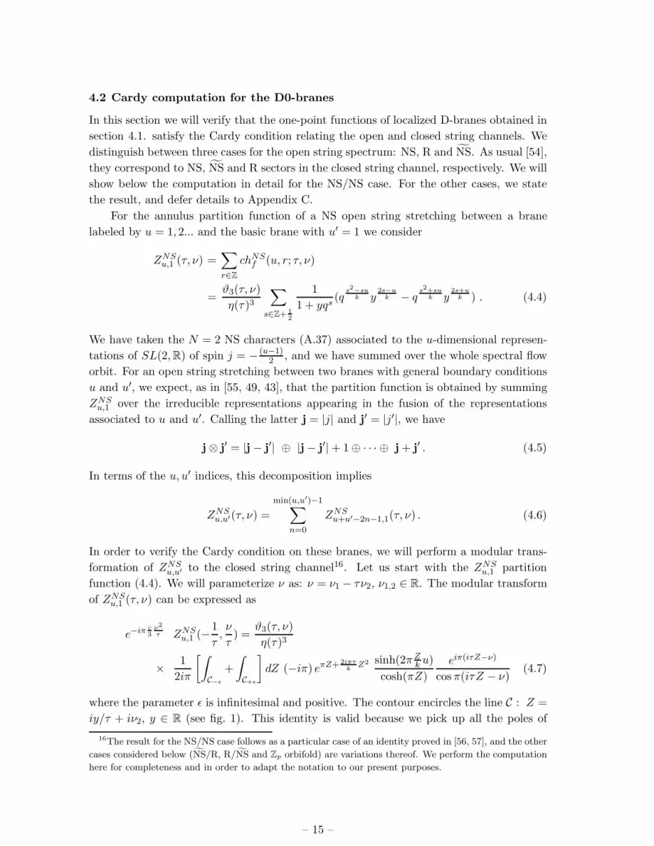
where the parameter ǫ is infinitesimal and positive. The contour encircles the line C : Z =

iy/τ + iν2, y ∈ R (see fig. 1). This identity is valid because we pick up all the poles of

16The result for the NS/NS case follows as a particular case of an identity proved in [56, 57], and the other

cases considered below (NS/R, R/NS and Zp orbifold) are variations thereof. We perform the computation

here for completeness and in order to adapt the notation to our present purposes.

– 15 –

C

C ε

−εX

X

XX

X

X

X

X

2 ε

X

CZ plane

X

X

X

X

X

2ν

Figure 1: Choice of contour of integration (for τ1 > 0).

the integrand inside the contour. These are the zeroes of cos π(iτZ − ν) which occur at

ν − iτZ = y + ν1 = s ∈ Z + 1/2. At these poles, the contour integral yields the residues

−2

τ

eiπ(s−ν)/τ sin(2π uk (s − ν)/τ) e−i2π(s−ν)2/(kτ)

eiπ(s−ν)/τ + e−iπ(s−ν)/τ, (4.8)

which lead to the identity (4.7). This identity is valid as long as there are no poles coming

from the cosh πZ factor on the contour of integration. These special cases occur only for

ν2 ∈ Z+1/2 and we assume that ν2 does not take these values. We now note that we have

the expansions:

eiπ(iτZ−ν)

2 cos π(iτZ − ν)=

∞∑

w=0

(−1)we−2πiw(iτZ−ν) for |e−i2π(iτZ−ν)| < 1 (4.9)

and

eiπ(iτZ−ν)

2 cos π(iτZ − ν)= −

−1∑

w=−∞

(−1)we−2πiw(iτZ−ν) for |e+i2π(iτZ−ν)| < 1 . (4.10)

The expansion (4.9) is valid in C+ǫ and (4.10) is valid in C−ǫ. Plugging these expansions

into the right hand side of eq. (4.7) we get

e−iπ c3

ν2

τ ZNSu,1 (−1

τ,ν

τ) =

ϑ3(τ, ν)

η(τ)3

∑

w∈Z

∫

CdZ (−1)w

sinh(2πZk u)

cosh(πZ)eπZ ywq−iwZ+ Z2

k . (4.11)

When taking ǫ→ 0 we added a minus sign to the contour C+ǫ and switched its direction. To

obtain the corresponding expression for the general case (4.6) of ZNSu,u′ , we use the identity

min(u,u′)−1∑

n=0

sinh

(2πZ

k(u+ u′ − 2n− 1)

)=

sinh(2πZk u) sinh(2πZ

k u′)

sinh(2πZk )

(4.12)

– 16 –

so we get

e−iπ c3

ν2

τ ZNSu,u′(−1

τ,ν

τ) =

ϑ3(τ, ν)

η(τ)3

∑

w∈Z

∫

CdZ (−1)w

sinh(2πZk u) sinh(2πZ

k u′)

cosh(πZ) sinh(2πZk )

eπZ ywq−iwZ+ Z2

k . (4.13)

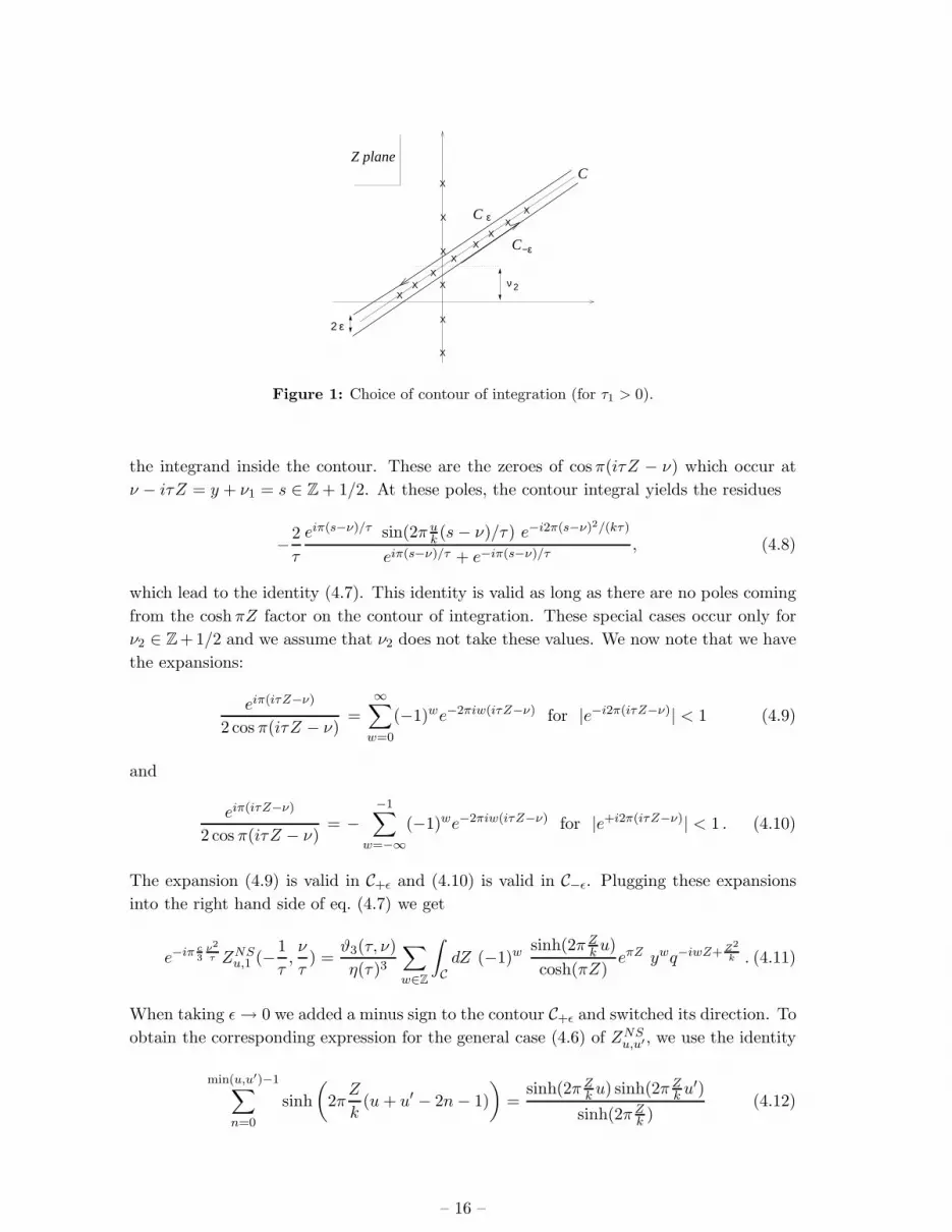
Note that the exponent of q is complex. In order to get a real exponent for q we will (i) shift

the C contour of integration by iwk2 − iν2, for each term indexed by w and (ii) tilt it parallel

to the real axis (see fig. 2). The resulting exponent of q will be that needed to get the

characters of the continuous representations. As we shift the contour we pick poles which

X

X

X

X

X

X

2

C

(i)

(ii)

ν

R + ikw/2

kw/2

Figure 2: Change of contour of integration (case w > kν2

2).

will make up the contributions of the N = 2 discrete representations to the closed string

channel amplitude. No poles are picked when tilting to the real axis. So the modular

transform of ZNSu,u′ is decomposed into

e−iπ c3

ν2

τ ZNSu,u′(−1

τ,ν

τ) = ZNS,c

u,u′ + ZNS,du,u′ . (4.14)

The first term comes from the continuous integral, which after shifting and tilting the

contour, becomes

ZNS,cu,u′ =

∑

w∈Z

∫ +∞

−∞dP

eπ( iwk2

+P ) sinh(2πPk u) sinh(2πP

k u′)

(−1)w(u−u′) cosh(π(P + iwk2 )) sinh(2πP

k )(4.15)

× qP2+(wk/2)2

k yw ϑ3(τ, ν)

η(τ)3.

In the last factor we get a continuous character chNSc (P, wk

2 ; τ, ν) (see (A.20)), correspond-

ing to a pure winding state with m = kw2 , as expected. And since chc(P,

wk2 ; τ, ν) is even

in P we can rewrite this as

ZNS,cu,u′ =

∑

w∈Z

∫ +∞

0dP

2 sinh(2πP ) sinh(2πPk u) sinh(2πP

k u′)

(−1)w(u−u′)[cosh(2πP )+cos(πkw)] sinh(2πPk )chNS

c (P,wk

2; τ, ν) .

(4.16)

– 17 –

This expression is equal to

ZNS,cu,u′ =

∑

w∈Z

∫ +∞

0dP Ψu

(1

2− iP,−w

)Ψu′

(1

2+ iP,w

)chNS

c (P,wk

2; τ, ν) (4.17)

so we get the expected continuous spectrum from the overlap between D0 boundary

states17.

The poles picked up arise from the zeroes of the factor cosh πZ in (4.13), at values of

Z such that Z = is with s ∈ Z + 12 . Note that for irrational k the shifted contour will

never fall on a pole, and we will assume this to be the case. The poles will contribute with

positive sign for s > ν2 and with negative sign for s < ν2. Let us consider the former case.

A given s ∈ Z + 12 will give a pole contribution for all the terms in (4.11) with w > ws,

where ws is the only integer satisfying

ws >2s

k> ws − 1 . (4.18)

For poles corresponding to s < ν2, we get contributions for all the terms in (4.11) with

w 6 ws − 1, where ws is also defined by (4.18). Summing all these residues we get

ZNS,du,u′ = −2

ϑ3(τ, ν)

η(τ)3

[∑

s>ν2

∞∑

w=ws

−∑

s<ν2

ws−1∑

w=−∞

]sin(2π s

ku)sin(2π s

ku′)

(−1)w sin(2π s

k

) ywqsw− s2

k . (4.19)

Noting that |yqs| = e−2πτ2(s−ν2) is smaller (bigger) than 1 for s > ν2 (s < ν2), we can sum

on w for every s to get

ZNS,du,u′ = −2

∑

s∈Z+ 12

(−1)wssin(2π s

ku)sin(2π s

ku′)

sin(2π s

k

) ywsqsws−s2

k

1 + yqs

ϑ3(τ, ν)

η(τ)3. (4.20)

This result can be recast in a more transparent fashion as follows. Calling s = r + 12

with r ∈ Z, a character of the N = 2 NS discrete representations corresponding to a pure

winding mode J30 = j + r = kw

2 is given by (see (A.31))

chNSd (j, r; τ, ν) =

ywqsw− s2

k

1 + yqs

ϑ3(τ, ν)

η(τ)3. (4.21)

Now, for every r ∈ Z there is only one value of w, such that j = −r + kw2 lies in the

improved unitary bound (2.7). This is exactly the value of w fixed by the condition (4.18).

Moreover, all possible representations corresponding to pure winding states and such that

j lies inside the unitary bound are covered by taking all r ∈ Z and fixing ws as in (4.18).

Calling jr the spin of the representation associated to each r, then (4.20) is equal to

ZNS,du,u′ =

∑

r∈Z

(−1)wr(u−u′) 2 sin(

πk (2jr − 1)u

)sin(

πk (2jr − 1)u′

)

sin(

πk (2jr − 1)

) chNSd (jr, r; τ, ν) (4.22)

17Note that in the ”out” boundary state we take the opposite U(1) charge, as follows from CPT conju-

gation [58].

– 18 –

where ws has been renamed wr.

As shown in section 4.1, the product Ψu(−j + 1,−w)Ψu′(j, w) has a single pole for

every discrete, pure-winding state. It is natural to expect the discrete part of the annulus

amplitude (in the closed string channel) to be given by the residue of this pole. This is

indeed the case, and one can check that (4.22) is equal to

ZNS,du,u′ = 2π

∑

r∈Z

Res[ΨNS

u (−jr + 1,−wr)ΨNSu′ (jr, wr)

]chNS

d (jr, r; τ, ν) , (4.23)

where the residue is computed when considering the bracketed expression as an analytic

function of j. More details about this last step are given in section 7 that treats D2-branes.

We have thus verified the Cardy consistency condition for the D0 branes in the NS/NS

sector.

The computation for the R/NS and NS/R cases is basically the same, mutatis mutandi.

We state here the results and provide the details of the computation in Appendix C for

the interested reader. For the open string sector we take the partition functions

ZRu,1(τ, ν) =

∑

r∈Z+ 12

chRf (u, r; τ, ν) , (4.24)

ZNSu,1 (τ, ν) =

∑

r∈Z

chNSf (u, r; τ, ν) , (4.25)

and ZR/NSu,u′ (τ, ν) is given by a sum as in (4.6). The modular transforms are

e−iπ c3

ν2

τ ZRu,u′(−1

τ,ν

τ) = (4.26)

∑

w∈Z

∫ +∞

0dP ΨNS

u

(1

2− iP,−w

)ΨNS

u′

(1

2+ iP,w

)chNS

c (P,wk

2; τ, ν)

+2π∑

r∈Z

Res[ΨNS

u (−jr + 1,−wr)ΨNSu′ (jr, wr)

]chNS

d (jr, r; τ, ν) ,

e−iπ c3

ν2

τ ZNSu,u′(−1

τ,ν

τ) = (4.27)

∑

w∈Z

∫ +∞

0dP ΨR

u

(1

2− iP,−w

)ΨR

u′

(1

2+ iP,w

)chR

c (P,wk

2; τ, ν)

+2π∑

r∈Z+ 12

Res[ΨR

u (−jr + 1,−wr)ΨRu′(jr, wr)

]chR

d (jr, r; τ, ν) ,

where jr and wr are defined in the same way as for the NS/NS case, but notice that in

the the R case r is half-integer. In both (4.26) and (4.27) the residues are again computed

considering the bracketed expression as a function of j.

Some comments are in order.

– 19 –

• Although the Cardy condition holds for arbitrary boundary conditions u, u′, there

are reasons to argue that only the u = u′ = 1 case corresponds to physical D-

branes. Firstly, for u, u′ 6= 1 the open string partition function is built from non-

unitary N = 2 representations. An alternative argument was given in [43], based

on comparing higher values of u to expectations for the physics of coinciding single

D0-branes.

• From the case of the D0 branes we draw an important lesson, which will remain

valid for the D1 and D2 branes. Although the open string partition function is built

out of N = 2 characters, the product of the one point functions in the closed string

channel is the same as that of the bosonic 2D black hole studied in [43] at level k+2.

Using identities developed in [57] (see also [59]) to relate sums of characters of N = 2

representations to characters of a bosonic SL(2,R)/U(1) model, one can expand the

partition function (4.4) of a string stretching between a u-brane and a basic brane as

ZNSu,1 (τ, ν) =

1

η(τ)

∑

n,r∈Z

z(j+r)k/2

+nq

k/2k+2

( (j+r)k/2

+n)2[λj,r−n(τ) − λ−j+1,r−n−u(τ)] (4.28)

where j = − (u−1)2 and

λj,r(τ) = η(τ)−2q−(j− 1

2 )2

k+ (j+r)2

k+2

∞∑

s=0

(−1)sq12s(s+2r+1) (4.29)

are the characters of the bosonic coset SL(2,R)/U(1) descending from bosonic SL(2,R)

primaries with J30 = j + r. On the other hand, the open string partition function

of a bosonic open string stretching between similar D-branes in the bosonic cigar

background is given by [43]

Zbosonicu,1 (τ, ν) =

∑

r∈Z

[λj,r(τ) − λ−j+1,r(τ)] . (4.30)

Notice that the partition functions (4.28) and (4.30) differ by characters of a U(1)

boson. This is the U(1) R-current of N = 2, who is responsible for the extension

of the bosonic SL(2,R)/U(1) algebra into N = 2 [23]. It is a free boson, and it

is coupled in a way that is of mild consequence to the modular matrix and to the

one-point functions.

5. D0 branes in a Zp orbifold

Before proceeding to the D1 branes, we will discuss a natural and interesting generalization

of the D0 branes considered in the previous section.

In the annulus partition function (4.4) we summed over the whole infinite spectral flow

orbit, and this was essential in order to obtain a discrete spectrum of U(1) charges in the

closed string channel. But a consistent result is also obtained if the sum is taken with

– 20 –

jumps of p units of spectral flow. As we will see, this correspond to D0 branes living in a

Zp orbifold of the original background, and in this framework we will be able to connect

with previous works on boundary N = 2 Liouville theory [10, 11, 12].

The orbifold acts freely as a shift of 2π/p on the angular direction of the cigar. As for

a compact free boson, we expect that the orbifold theory is equivalent to the original one

with the radius divided by p. This implies a spectrum of charges given by

J30 + J3

0 = m+ m =kw

p, J3

0 − J30 = m− m = pn. (5.1)

Moreover, since the (infinite) volume of the target space decreases now by a factor 1/p, we

expect that the one point functions should be renormalized by√

1/p. For k integer one

can mod out the theory by Zk (see below), and we get the spectrum of single cover of the

vector coset SL(2,R)/U(1) [25], which has the target space geometry of the trumpet, at

first order in 1/k.

By applying the same method of descent from H+3 we can compute the one-point

function for this orbifold. For simplicity, we will study here the NS/NS case, with u = u′ =

1, and we omit the NS/u/u′ labels.. The other sectors are similar.

We obtain the following one-point function for the D0-branes :

Ψp,a(j, w) =1√pke−2πiaw

p ν12−j

Γ(j + kw2p )Γ(j − kw

2p )

Γ(2j − 1)Γ(1 − 1−2jk )

(5.2)

where a ∈ Zp is an additional quantum number of these D-branes and the phase e−2πiawp

is fixed by the Cardy condition.

Let us start with the open string partition function for an open string stretching

between two such D0-branes, for which we consider

Zp;a,a′(τ, ν) =∑

r∈Zp+a−a′

chf (1, r; τ, ν)

=ϑ3(τ, ν)

η(τ)3

∑

s∈Zp+a−a′+ 12

qs2−s

k y2s−1

k

1 + yqs−

∑

s∈Zp−1+a−a′+ 12

qs2+s

k y2s+1

k

1 + yqs

. (5.3)

We have summed over all the representations of the spectral flow with p-jumps, with the

starting point r = a− a′ coming from the additional parameters of these D0-branes.

In order to check the Cardy condition, we will perform a modular transformation of

Zp;a,a′ to the closed string channel. The computation is very similar to that of the previous

section, so we will indicate only the major steps. We start with

e−iπ c3

ν2

τ Zp;a,a′(−1

τ,ν

τ) =

ϑ3(τ, ν)

η(τ)3× (5.4)

1

2iπ

[∫

C−ǫ

+

∫

C+ǫ

]dZ

(−iπ)

p

eπZ+2π Zk

+ 2iπτk

Z2

cosh(πZ)

e−iπ( ν−iτZ−1/2−(a−a′)

p+ 1

2)

2 cos π(ν−iτZ−1/2−(a−a′)p + 1

2)

− 1

2iπ

∫

C−ǫ

+

∫

C+ǫ

]dZ

(−iπ)

p

eπZ−2π Zk

+ 2iπτk

Z2

cosh(πZ)

e−iπ(ν−iτZ+1/2−(a−a′)

p+ 1

2)

2 cos π(ν−iτZ+1/2−(a−a′)p + 1

2 )

.

– 21 –

The contour of integration is the same as in the previous section, but now the last factor

of the integrand has poles at values ν − iτZ = pZ + a − a′ + 12 in the first term, and at

ν−iτZ = pZ+a−a′− 12 for the second. Expanding the last factor of (5.4) as in (4.9)-(4.10),

and taking ǫ→ 0 in the contours C±ǫ, yields,

e−iπ c3

ν2

τ Zp;a,a′(−1

τ,ν

τ) =

ϑ3(τ, ν)

η(τ)3

∑

w∈Z

∫

CdZ e

−2iπ(a−a′)wp

sinh(π(2Zk − iw

p ))

p cosh(πZ)eπZ y

wp q

−i wZp

+ Z2

k . (5.5)

In order to express (5.5) as a sum over characters we shift the contour in each term by an

amount of iwk2p − iν2. As in the previous section, we pick poles for Z = is, with s ∈ Z + 1

2 ,

corresponding to the discrete representations. Defining ws ∈ Z as

ws >2ps

k> ws − 1 , (5.6)

the poles with s > ν2 (s < ν2) are picked with positive (negative) sign, by all the values

w ≥ ws (w < ws) in (5.5). The sum of all the poles is

−2ϑ3(τ, ν)

η(τ)3

[∑

s>ν2

∞∑

w=ws

−∑

s<ν2

ws−1∑

−∞

]e−2πi(a−a′)w

p sin

(2πs

k− πw

p

)y

wp q

swp− s2

k (5.7)

= −2ϑ3(τ, ν)

η(τ)3

∑

s∈Z+ 12

∑

n∈Zp

e−2πi(a−a′)ws+np sin

(2πs

k− π

(ws + n)

p

)y

ws+np q

s(ws+n)p

− s2

k

1 + yqs.

Collecting the continuous and discrete contributions, we get finally

e−iπ c3

ν2

τ Zp;a,a′(−1

τ,ν

τ) = (5.8)

∑

w∈Z

∫ +∞

0dP Ψp,a′

(1

2− iP,−w

)Ψp,a

(1

2+ iP,w

)chNS

c (P,kw

2p; τ, ν)

+2π∑

r∈Z

∑

n∈Zp

Res[Ψp,a′(−jr,n + 1,−ws − n)Ψp,a(jr,n, ws + n)

]chNS

d (jr,n, r; τ, ν) ,

where as usual the residue is computed when considering the bracketed expression as a

function of j. The spins jr,n of the discrete representations are defined through

jr,n + r =k(ws + n)

2p(5.9)

where s = r+ 12 , and jr,n satisfies the unitary bound (2.7). Moreover, from (5.6) it follows

that the width k/2 of the unitary bound (2.7) is sliced into p intervals, and for each n ∈ Zp

we have

1

2+kn

2p< jr,n <

k(n + 1)

2p+

1

2. (5.10)

Finally, note that the choice of a in the open string channel, which is a statement about

the spectrum, becomes a phase in the closed string channel.

– 22 –

The Zk and Z∞ cases

In this context, we can now construe previous studies of D-branes in N = 2 Liouville theory

as particular cases of the orbifold discussed here.

In [10] D-branes were built in a N = 2 model with rational central charge c = 3 + 6KN ,

with K,N positive integers, and the D0-brane open string partition function was taken

with jumps of N spectral flow units (for u = u′ = 1). This corresponds to level k = NK

and p = N in our case. In particular, for K = 1, the asymptotic radius shrinks from

R =√kα′ to R

k = α′

R , which is the T-dual radius18. Indeed, notice that for p = k, the

spectrum of pure winding modes in (5.1) becomes pure momentum in the T-dual picture.

Note that we strengthen some of the results in [10], since our construction is explicitly

based on branes which have been checked to satisfy factorization constraints in the parent

theory [49]. Moreover, our results our based on a systematic analysis of a solution to the

branes preserving the full chiral algebra in the parent theory, and do not depend on the

central charge being rational. Apart from these bonuses, we also clarified the connection

to the semi-classical geometrical (mirror) cigar-picture.

Another interesting case to consider is the limit p→ ∞. This corresponds to the cigar

radius shrinking to zero, so that the spectrum (5.1) of m for pure winding states becomes

continuous, thus yielding a continuum of R-charges in the closed string channel. As shown

in [25] it corresponds to the vector gauging of the universal cover of SL(2,R).

At the level of the Cardy computation, naively taking the limit p → ∞ in (5.8) gives

zero in the closed string channel, since Ψp,a(j, w) goes to zero, see (5.2). The correct way

of proceeding is to notice that equation (5.5) becomes a Riemann sum, which leads to an

integral over t = wp ∈ R. We can moreover express t = x+ g, g ∈ Z, x ∈ [0, 1). The sum

over w in (5.5) becomes

1

p

∑

w

−→∫ +∞

−∞dt −→

∫ 1

0dx∑

g∈Z

. (5.11)

One can show that the resulting expression for the closed string channel is equivalent to

starting with

Z1,1(x; τ, ν) =∑

r∈Z

e2πixrchNSf (1, r; τ, ν) , (5.12)

and computing

∫ 1

0dx e−2πixde−iπ c

3ν2

τ Z1,1(x,−1

τ,ν

τ) , (5.13)

where d ∈ Z depends on the precise way the limit is taken in (5.11). The computation

of (5.13) itself can be performed with an identity proved in [56, 57], to which we refer for

details. The resulting expression can be found in [12].

18In the case of rational k there will be additional discrete terms in the closed string channel partition

function, coming from poles falling exactly on the displaced contour of section 4. But taking them into

account does not change the orbifold picture.

– 23 –

6. D1 branes

In this section, we check the relative Cardy condition for D1-branes in the N = 2 Liou-

ville/supersymmetric coset conformal field theory. In this and the next sections, we will

work in the NS sector. The other sectors are obtained straightforwardly. Following the

general logic, we assume that the one-point functions for closed string primaries in the

presence of a D1-brane labeled by the parameters (r, θ0) is given by (see Appendix B):

〈Φjnw(z, z)〉D1

r,θ0= δw,0

Ψr,θ0(j, n)

|z − z|∆j,n, (6.1)

with

Ψr,θ0(j, n) = N1einθ0

{e−r(−2j+1) + (−1)ner(−2j+1)

}ν

12−j Γ(−2j + 1)Γ(1 + 1−2j

k )

Γ(−j + 1 + n2 )Γ(−j + 1 − n

2 )

(6.2)

We put a normalization factor N1 up front that will be fixed during the Cardy computation.

Note that the only poles in the one-point function originate from infinite volume diver-

gences (i.e. they are bulk poles). Thus the only contributions to the closed string channel

amplitude between two D1-branes originate from continuous representations (unlike the

D0- and D2-brane computations where poles associated to discrete representations require

special attention). The closed string channel amplitude will only contain contributions

proportional to the continuous character:

chNSc (P,

n

2;−1

τ,ν

τ) = q

P2

k+ n2

4k ynkϑ3(− 1

τ ,ντ )

η3(− 1τ )

. (6.3)

We compute the closed string channel amplitude between two branes with identical bound-

ary conditions both labeled by (r, θ0), for simplicity. The computation can then easily be

generalized to include the case of differing boundary conditions, following [60]. For our

case, we find the partition function:

ZD1r,θ0

=

∫ ∞

0dP∑

n∈Z

Ψr,θ0(P, n)Ψr,θ0(−P,−n) chNSc

(P,n

2;−1

τ,ν

τ

)(6.4)

=4N 2

1

k

∫ ∞

0dP

1

sinh 2πP sinh 2πPk(

∑

n∈2Z

cos2 2rP cosh2 πP chNSc (P,

n

2) +

∑

n∈2Z+1

sin2 2rP sinh2 πP chNSc (P,

n

2)

).

We modular transform the characters to obtain the annulus amplitude suitable for inter-

pretation in the open string channel:

e−ciπν2

3τ ZD1r,θ0

=8N 2

1

k

∫ ∞

0dP

∫ ∞

0dP ′

∑

w∈ Z

2

cos4πPP ′

k

×cos2 2rP cosh2 πP + (−1)2w sin2 2rP sinh2 πP

sinh 2πP sinh 2πPk

chNSc (P ′, kw; τ, ν).(6.5)

– 24 –

Since the transformation properties of continuous N = 2 characters are analogous to the

transformation properties of purely bosonic coset characters, we can discuss the results sim-

ilarly as for the bosonic coset [43]. To make the discussion more explicit, and in particular

to match on to the boundary reflection amplitude, we follow [49, 43] to check the relative

Cardy condition. We compare the regularized density of states obtained in the open string

channel with the one we expect from a reflection amplitude which is the natural N = 2

generalization of the reflection amplitude in [49, 60, 43] (which satisfies factorization). To

this end, we subtract a reference amplitude labeled by r∗, and use trigonometric identities

and the change of variables t = 2πP to obtain:

e−ciπν2

3τ (ZD1r,θ0

− ZD1r∗,θ0

) =8N 2

1

k

∫ ∞

0dP ′

∑

w∈ Z

2

chNSc (P ′, kw) × (6.6)

∂

∂P ′

∫ ∞

0

dt

t

k

16π

cosh2 t2 − (−1)2w sinh2 t

2

sinh t sinh tk

{sin

2t

k(P ′ +

rk

π) + sin

2t

k(P ′ − rk

π) − (r → r∗)

}.

To link the relative density of continuous states in the open string channel to the boundary

reflection amplitude it is convenient to define the special functions:

logS(0)k (x) = i

∫ ∞

0

dt

t

(sin 2tx

k

2 sinh tk sinh t

− x

t

),

logS(1)k (x) = i

∫ ∞

0

dt

t

(cosh t sin 2tx

k

2 sinh tk sinh t

− x

t

). (6.7)

We can then write our ansatz for the boundary reflection amplitudes as:

R(P,w ∈ Z|r) = νiPk

Γ2k(−1

2 − iP + k)Γk(2iP + k)S(0)k (P + rk

π )

Γ2k(

12 + iP + k)Γk(−2iP + k)S

(0)k (−P + rk

π )

R(P,w ∈ Z +1

2|r) = νiP

k

Γ2k(−1

2 − iP + k)Γk(2iP + k)S(1)k (P + rk

π )

Γ2k(

12 + iP + k)Γk(−2iP + k)S

(1)k (−P + rk

π ). (6.8)

For the definition of the generalized gamma-functions Γk, we refer to e.g. [43] – they

immediately drop out of the computation of the relative partition function. Using the

reflection amplitudes (and the fact that they are parity odd) we can show that the relative

Cardy condition holds:

e−ciπν2

3τ (ZD1r,θ0

− ZD1r∗,θ0

) =N 2

1

πi

∫ ∞

0dP ′

∑

w∈Z

(∂

∂P ′log

R(P ′, w|r)R(P ′, w|r∗)

)chNS

c (P ′, kw)

+∑

w∈Z+ 12

(∂

∂P ′log

R(P ′, w|r)R(P ′, w|r∗)

)chNS

c (P ′, kw)

. (6.9)

To obtain agreement with the density of states expected on the basis of the boundary

reflection amplitude, we can fix N 21 = 1/2. Notice that in the open string channel, a pure

– 25 –

winding state has J30,open = 2J3

0,closed = kw. So we get in (6.9) contributions from open

strings winding both integer and half-integer times around the cigar. This is consistent

with the semiclassical geometry of the D1 branes in the cigar [43].

We have thus verified that the relative Cardy condition is satisfied by our D1-branes.

In summary, in this section we have argued that the relative Cardy condition holds, given

the one-point functions for the D1-branes we started out with, and the extension of the

boundary reflection amplitudes of [49, 60] to N = 2 theories. The computation follows the

lines of [43] due to the close connection between (continuous) N = 2 characters and those

of the bosonic coset, and their modular properties (see comment at the end of Section 4).

Note that the D1-branes couple to continuous bulk states with zero winding only.

7. D2-branes

In this section, we analyze the Cardy condition for the D2-branes which we can construct

from the H2 branes in Euclidean AdS3. They correspond to type B branes w.r.t. the

N=2 superconformal algebra. We find some puzzling features when trying to perform the

Cardy check. Following [43] and the general logic outlined before, we propose the following

one-point function for the D2-branes parameterized by σ, in the NS sector :

〈Φjnw(z, z)〉D2

σ = δn,0Ψσ(j, w)

|z − z|∆j,w, with :

Ψσ(j, w) = N2 ν12−j Γ(j + kw

2 )Γ(j − kw2 )

Γ(2j − 1)Γ(1 − 1−2jk )

eiσ(1−2j) sinπ(j − kw2 ) + e−iσ(1−2j) sinπ(j + kw

2 )

sinπ(1 − 2j) sin π 1−2jk

(7.1)

This one point function has poles corresponding to the discrete representations, and there-

fore will couple both to localized and extended states. This is expected on general grounds

since these D2-branes carry D0-brane charge.

The annulus partition function in the closed string channel, for general Casimir labeled

by j, in the NS sector, is:

ZD2σσ′ (−1/τ, ν/τ) = −kN 2

2

∫dj∑

w∈Z

chNS(j, kw

2 ;−1/τ, ν/τ)

sinπ(1 − 2j) sin π (1−2j)k

(7.2a)

{2 cos(σ + σ′)(1 − 2j) − 2 cos(σ − σ′)(1 − 2j) cos 2πj (7.2b)

+2 cos(σ − σ′)(1 − 2j) sin2 2πj

cos πkw − cos 2πj− 2i sin(σ − σ′)(1 − 2j) sin 2πj sinπkw

cos πkw − cos 2πj

}

(7.2c)

We can read from this expression that the different terms will contribute in a very different

fashion.

7.1 D1-like contribution

The two terms of the second line (7.2b) will give a contribution similar to the D1-branes

(which is an expected contribution, on the basis of the fact that the D2-branes also stretch

– 26 –

along the radial direction), with imaginary parameter though. Explicitely, we have in the

closed channel :

ZD2,(b)σσ′ (−1/τ, ν/τ) = 2kN 2

2

∫ ∞

0dP∑

w∈Z

chNSc

(P, kw

2 ;−1/τ, ν/τ)

sinh 2πP sinh 2πP/k[cosh 2P (σ + σ′) + cosh 2P (σ − σ′) cosh 2πP

]. (7.3)

As for the D1-branes, we consider the relative partition function w.r.t. the annulus ampli-

tude for reference branes of parameters (σ0, σ′0). Going through the same steps as in the

previous sections, we obtain the open string channel amplitude :

ZD2,(b)σσ′ (τ, ν) = 4kN 2

2

∫dP ′ ∂

2iπ ∂P ′log

{R(P ′|iσ+σ′

2 ) R(P ′|iσ−σ′

2 )

R(P ′|iσ0+σ′0

2 ) R(P ′|iσ0−σ′0

2 )

}∑

n∈Z

chNSc (P ′, n; τ, ν)

(7.4)

in terms of reflections amplitudes similar as before, see (6.8), but with imaginary parameters

i(σ ± σ′)/2 . We fix the normalization constant to N 22 = 1

4k .

7.2 D0-like contribution

Now we concentrate on the last two terms (7.2c) of the annulus amplitude. As we will see

this will give a contribution similar to those of D0-branes, hence with both discrete and

continuous contributions. Let’s first concentrate on the latter. Since the last term is odd

in w, it will cancel from the amplitude19 and we are left with :

ZD2,(c)σσ′, cont(−1/τ, ν/τ) = −1

2

∫ ∞

0dP∑

w∈Z

cosh 2P (σ − σ′) sinh2 2πP chNSc

(P, kw

2 ;−1/τ, ν/τ)

(cosh 2πP + cos πkw) sinh 2πP sinh 2πP/k

(7.5)

Assuming that σ − σ′ = 2πm/k, m ∈ Z, we recognize a D0 amplitude for two branes of

same parameter m :

ZD2,(c)σσ′, cont

(−1

τ,ν

τ

)= −1

2

∫ ∞

0dP∑

w∈Z

(2 sinh2(2πPm/k) + 1

)sinh 2πP

(cosh 2πP + cos πkw) sinh 2πP/k

× chNSc

(P,kw

2;−1/τ, ν/τ

), (7.6)

up to the constant term in the bracketed expression, that will drop from the relative

partition function. The normalization −1/2 of this expression has to be compared with

the normalization (−)w(m−m) = 1 of the D0 computation (4.16).

Discrete representations

We can also make the identification with a D0-like contribution as follows. First we consider

the more straightforward case w > 0. Then we pick the poles of the discrete representations

19Strictly speaking, this holds only when ν = 0. The same is true in the discrete sector below.

– 27 –

in the domain : j ∈ D =(

kw2 − N

)∩]

12 ; k+1

2

[. For each pole we will have a contribution

of 2π times the residue :

−1

2

∑

j∈D

∑

w>0

(−)j−kw2

cos 2πm2j−1k sinπ(2j − 1) − i sin 2πm2j−1

k sinπkw

sinπ(j + kw2 ) sinπ 2j−1

k

chNSd (j,−kw/2− j)

(7.7)

We write j = kw2 − r, with r ∈ N. Then for every r, there is only one value of w, that we’ll

call wr such that j is in the correct range. Explicitely wr is given by: wr = ⌊2r+1k ⌋+1. We

call also jr the value of j that has been picked. With this procedure we get :

−1

2

∑

r∈N

(−)wrcos 2πm2r+1

k − i sin 2πm2r+1k

sinπ 2r+1k

chNSd (jr, r) (7.8)

Let us now consider the case w 6 0. In this case we have to use the isomorphism of

representations : D+,wj ≃ D−,w−1

j′ , with j′ = k+22 − j. We have then j′ = −k

2 (w − 1) − r′,

r′ ∈ N, and the value of w is fixed to : wr′ = −⌊2r′+1k ⌋. This leads to the following

contribution to the annulus amplitude:

−1

2

∑

r′∈N

(−)w′r−1 cos 2πm2r′+1

k + i sin 2πm2r′+1k

sinπ 2r′+1k

chNSd (j′r′ ,−r′) (7.9)

Then it is possible to add the two contributions, which cancels the imaginary part, and

leaves us with :

ZD2,(c)σσ′, disc

(−1

τ,ν

τ

)= −1

2

∑

r∈Z

(−)⌊2r+1

k⌋ 2 sin2 2πm r+1/2

k − 1

sin 2π r+1/2k

chNSd

(jr, r;−

1

τ,ν

τ

). (7.10)

This is again −1/2 of the expression of the amplitude for two D0’s of parameter m,

eq. (4.22), up to the irrelevant constant term.

Some comments on D2-branes physics

The following comments are in order:

• in the computation we assumed that the difference of the parameters of the D2 in the

annulus amplitude is quantized: σ′ − σ = 2πm/k, m ∈ Z. This relative quantization

condition is discussed in [43] for the bosonic coset. Indeed the difference of the D2-

branes parameters is the net induced D0-charge, hence it should be quantized. To be

more precise it is believed that a D2-brane with parameter σ′ is a bound state of a

brane of parameter σ with m D0-branes (for the σ′ > σ case , otherwise one has to

reverse the picture)

• as a corollary, the one-point functions for the D2-branes have poles both of the local-

ized type and of the bulk type

• the computation of the annulus amplitude gives a continuous spectrum of open strings

attached to the D2-branes, with a sensible density of states, and also a contribution

– 28 –

similar to the D0 – see the previous remark about the induced D0 charge – but

with a normalization (−1/2) which complicates the task of making sense of the open

string spectrum, and blurs the physical picture of bound states. The only open

string spectrum leading to a good physical picture would seem to correspond to two

D2-branes with the same parameter σ.

Clearly further study of the physics of D2-branes is needed to clarify their interpretation.

8. Conclusions

We constructed D-branes in N = 2 Liouville theory and the SL(2,R)/U(1) super-coset

conformal field theory, and checked the (relative) Cardy condition as well as consistency

with the proposed boundary reflection amplitudes, which were proven earlier to satisfy the

factorization constraints. The one-point functions that we constructed remarkably decou-

ple the poles in bulk amplitudes (notably the reflection amplitude) into poles associated to

infinite volume and the ones associated to normalizable discrete states. It would be inter-

esting to investigate whether the boundary decoupling phenomenon aids in understanding

more aspects of the conjectured holographic duality in the (doubly scaled) little string

theory.

We have shown (for the particular but extendable) case of the D0-branes how to

generalize the results to other sectors of the supersymmetric Hilbert space, and to orbifolds

of the cigar conformal field theory.

We have pointed out throughout this work some similarities of the one-point functions

for N = 2 Liouville with those of the N = 0, 1 cases, like the decoupling of the bulk poles.

It would be interesting to see also whether the interesting relations uncovered in [61, 62]

between the boundary states associated to localized and extended branes have also any

manifestation in the N = 2 theory.

In appendices, we argued for the general use of the SL(2,R) symmetry that can be

obtained by enhancing N = 2 theories with an orthogonal free scalar, and we suggested

that this tool provides some technical support for an attempt to interpret the variables

(x, x) – parameterizing the SL(2,R) quantum numbers in position space on the boundary

of AdS3 – as new worldsheet variables. We showed in great detail the fact that super-

coset characters agree with N = 2 characters, and the N = 2 spectral flow has a natural

interpretation in terms of SL(2,R) quantum numbers.

Note that we have constructed D-branes for generic values of the level k. It is known

that the conformal field theory correlators depend strongly on whether k is rational or

irrational (for instance via the shift equations, or the structure of the poles in the bulk

correlators). It seems important to further clarify the relation between the construction

of branes at rational and irrational values of k (for instance by further comparing the

techniques developed in [57] to the results of [43]), as well as the dependence of bulk

correlators on this most intriguing distinguishing feature.

The branes we constructed form an integral part of the construction of D-branes in non-

compact non-trivially curved supersymmetric string theory backgrounds. One particular

– 29 –

application amongst these is the construction of D1-branes and D3-branes in the Little

String Theory background in the double scaling limit (see also e.g. [63, 64, 65]). Indeed,

when we consider the doubly scaled limit for NS5-branes which are evenly distributed over

a topologically trivial circle, we obtain a closed string background which is supposed to

represent a holographic dual of the Higgs phase of the Little String Theory living on the

NS5-branes [5], whose partition function has been studied in [26, 8]. The role of the W-

bosons in the LST is played by the D1-branes stretching between the NS5-branes. One can

construct at least the one-point functions corresponding to these D-branes by combining the

D0-brane in the SL(2,R)/U(1) theory and a D1-brane in the supersymmetric SU(2)/U(1)

coset theory, properly taking into account the discrete orbifold operation. The construction

of these one-point functions is now straightforward. We will return to some of these issues

in the near future [66].

Acknowledgments

We thank Shmuel Elitzur, Angelos Fotopoulos, Stefan Fredenhagen, Gaston Giribet, Amit

Giveon, Anton Kapustin, Elias Kiritsis, Costas Kounnas, David Kutasov, Marios Petropou-

los, Boris Pioline, Sylvain Ribault, Adam Schwimmer and especially Volker Schomerus for

comments and discussions. AP thanks the Laboratoire de Physique Theorique de l’Ecole

Normale Superieure for hospitality during the first part of this work, and the organizers of

the ESI Workshop ”String Theory in Curved Backgrounds and Boundary Conformal Field

Theory”. AP is supported by the Horowitz Foundation and by an ESI Junior Fellowhip.

This work is supported in part by the Israeli Science Foundation and by the EEC under

the contracts HPRN-CT-2000-00122, HPRN-CT-2000-00131.

A. Computing N=2, c>3 characters

In this appendix we will compute the N = 2, c > 3 characters appearing in the spectrum of

the D-branes studied in the paper. We will obtain them as characters of the supersymmetric

coset SL(2,R)/U(1), through a rather standard procedure. The same characters can be

computed by subtracting the null-vectors modules from the free action of the N = 2

generators, as has been done in [67, 68, 69]. The N = 2 representations that we consider

are both unitary and non-unitary. The characters of the former have been computed in

those papers and coincide with our results, while for non-unitary representations we present

the characters for the first time. The fact that the coset yields irreducible N = 2 characters

can be traced back to the fact that the SL(2,R) characters we start with correspond to

irreducible representations of the SL(2,R) algebra.

Notice that we have here a non-minimal version of a similar situation for (N = 1, 2

supersymmetric) unitary minimal models, where the (supersymmetric) Virasoro characters

coincide with the characters of certain cosets involving SU(2) factors which realize the

minimal models [70].

Moreover, this coincidence of the two ways of computing the characters, which was

independently noticed in [26] and [8], is central to the fact that the D-branes that we build

– 30 –

in this paper belong to the class of objects, such as the correlation functions [4, 35, 32]

or the modular-invariant partition function [26, 8], for which there is no distinction as to

whether we are in the N = 2 Liouville or in the supersymmetric cigar.

Let us review first how the N = 2 algebra arises in the susy SL(2,R)/U(1) coset [3].

The supersymmetric SL(2,R) model at level k has currents Ja, ψb (a, b = 1, 2, 3), with

OPEs

Ja(z)Jb(w) ∼ gabk/2

(z − w)2+fab

c Jc(w)

z − w,

Ja(z)ψb(w) ∼ fabcψ

c(w)

z − w,

ψa(z)ψb(w) ∼ gab

z − w(A.1)

where gab = diag(+,+,−), f123 = 1 and indices in the antisymmetric fabc are raised and

lowered with gab.

We first define

ja = Ja − Ja

Ja = − i

2fa

bcψbψc (A.2)

The currents ja commute with the three fermions and generate a bosonic SL(2,R) model

at level k + 2. The currents Ja, ψa form a supersymmetric SL(2,R) model at level −2.

The Hilbert space of the original supersymmetric SL(2,R)k theory is the direct product of

the Hilbert space of the bosonic SL(2,R)k+2 and that of the three free fermions.

We are interested in the coset obtained by gauging the U(1) symmetry generated by

J3, ψ3. This coset has an N = 2 algebra generated by

G± =

√2

kψ±j∓

JR =2

kj3 +

k + 2

kJ3 =

2

kJ3 + ψ+ψ− (A.3)

T = TSL(2,R) − TU(1)

where√

2ψ± = ψ1 ± iψ2 and

TU(1) = −1

kJ3J3 +

1

2ψ3∂ψ3 . (A.4)

The currents (A.3) commute with J3, ψ3 and satisfy the N = 2 superconformal algebra

JR(z)JR(w) ∼ c/3

(z − w)2,

JR(z)G±(w) ∼ ± G±(w)

(z − w),

G+(z)G−(w) ∼ 2c/3

(z − w)3+

2JR(w)

(z −w)2+

1

(z − w)

(2T (w) + ∂JR(w)

).

(A.5)

– 31 –

with the central charge

c = 3 +6

k. (A.6)

A highest-weight representation of the N = 2 algebra with a given central charge c is

determined by the conformal dimension h and the U(1) charge Q of the highest weight

state. By building the N = 2 representations through the SL(2,R)/U(1) coset, we can

parameterize h,Q by means of SL(2,R) quantum numbers as follows from the zero modes

of J3, T in (A.3).

The states of the coset are all those states in the parent SL(2,R) theory annihilated

by the modes J3n>0, ψ

3n>0, and a primary state of the coset is a coset state which is also

a primary of the N = 2 algebra. Every primary state of the parent theory is clearly a

primary of the coset. In addition, for the discrete and finite-dimensional representations of

ja, there are also descendent states of the parent theory which are primaries of the coset.

The Hilbert space of the parent theory can be decomposed into subspaces with definite

J30 eigenvalue m. Since the N = 2 algebra commutes with J3

0 , from a given SL(2,R)

representation with spin j, we will obtain a different N = 2 representation for each value

of m. The use of j,m labels is most convenient, because performing integer spectral flow

in N = 2 just amounts to an integer shift in m, as we will see below.

For a given SL(2,R) representation, we are interested in the characters

chNSj,m(q, y) = q−

c24 TrNS qL0yJR

0 (A.7)

chNSj,m(q, y) = q−

c24 TrNS (−1)F qL0yJR

0 (A.8)

chRj,m(q, y) = q−

c24 TrR qL0yJR

0 (A.9)

where the trace is taken on the Hilbert space of the coset. We will compute in all the cases

the NS character first. The Ramond characters will be obtained by half-spectral flow [71]

as

chR(τ, ν) = qc6( 12)2y

c3

12 chNS(τ, ν +

τ

2) (A.10)

where q = ei2πτ , y = ei2πν . As for the NS characters, it is easy to see that they are given

by

chNSj,m(τ, ν) = eiπQj,mchNS

j,m(τ, ν − 1/2) (A.11)

where Qj,m is the U(1) charge of the highest weight state. The NS characters can be

obtained from

χj(q, x, y) = Tr qL0−c+3/2

24 xJ30 yJR

0 =∑

m

xm ξm(q) chNSj,m(q, y) (A.12)

where

ξm(q) = q−348

−m2

k

∞∏

n=1

(1 + qn− 12 )

(1 − qn)(A.13)

– 32 –

The trace in (A.12) is taken on the whole NS Hilbert space of the supersymmetric SL(2,R)kmodel and JR

0 is well-defined even before going to the coset. We have expanded χj(q, x, y)

into terms with definite J30 charge m and factored in each such term a supersymmetric

U(1) character ξm(q) with highest weight ∆ = −m2

k , generated by the modes of J3, ψ3.

The computation of χj(q, x, y) itself goes as follows. In the factorized SL(2,R)k+2 ⊗{ψa} theory we can easily compute

χj(q, z, w) = q−c+3/2

24 Tr qL0zj30 × Tr qL0wJ3

0 , (A.14)

and then from (A.2) and (A.3) it follows that χj(q, x, y) is given from χj(q, z, w) by the

replacements

z → xy2k ,

w → xyk+2

k . (A.15)

In (A.14), the trace over the fermions NS Hilbert space is

Tr qL0wJ30 =

∞∏

n=1

(1 + qn− 12 )(1 + wqn− 1

2 )(1 + w−1qn− 12 )

=∞∏

n=1

(1 + qn− 12 )

(1 − qn)

∑

p∈Z

wpqp2

2 . (A.16)

For the first factor in (A.14), we should consider the different possible representations of

the ja algebra. We take q = ei2πτ , y = ei2πν .

Continuous representations

The ja representations are built by acting with jan<0 on representations of the zero modes ja0 .

For the continuous representations we have j = 12 + iP , P ∈ R

+. The SL(2,R) primaries

are |P,m〉, with m = r + α, r ∈ Z, α ∈ [0, 1) and conformal weight

−j(j − 1)

k=

14 + P 2

k. (A.17)

These primaries of ja are multiplied by the fermionic NS vacuum to get the full primaries,

so j30 = J30 = m on these states. Considered as primaries of N = 2, they give rise to unitary

N = 2 representations [23] with (see (A.3))

hP,m =14 + P 2 +m2

k, Qm =

2m

k(A.18)

The character of the susy SL(2,R) representation is

χj(q, z, w) = q−c+3/2

24 Tr qL0zj30 × Tr qL0wJ3

0 ,

= q−c+3/2

24 q1/4+P2

k

∑

r,p∈Z

zα+rwpqp2

2

∞∏

n=1

(1 + qn− 12 )

(1 − qn)4(A.19)

– 33 –

and applying the steps described above it is immediate to obtain the N = 2 characters

chNSc (P,m; τ, ν) = Tr qL0−c/24 yJR

0

= qP2+m2

k y2mkϑ3(τ, ν)

η(τ)3(A.20)

chNSc (P,m; τ, ν) = q

P2+m2

k y2mkϑ4(τ, ν)

η(τ)3(A.21)

chRc (P,m′; τ, ν) = q

P2+m′2

k y2m′

kϑ2(τ, ν)

η(τ)3(A.22)

wherem′ = m+ 12 when the Ramond character is obtained by half-spectral flow from (A.20).

Discrete representations

Let us consider discrete lowest-weight representations D+j of ja, with primaries |j, r〉, with

m = j + r and r ∈ Z, r > 0, and with j ∈ R, j > 0. For 0 < j < k+22 they give rise to

N = 2 unitary representations [72, 23, 73]. This bound is further constrained in physical

settings to be 12 < j < k+1

2 . For each value of m = j + r, r ∈ Z the N = 2 primaries are

r ≥ 0 |j, j + r〉r < 0 (j−−1)

−r−1ψ−− 1

2

|j, j〉 (A.23)

The quantum numbers are:

r ≥ 0 hj,r = −j(j−1)+(j+r)2

k Qj,r = 2(j+r)k

r < 0 hj,r = −j(j−1)+(j+r)2

k − r − 12 Qj,r = 2(j+r)

k − 1

=−(k+2

2−j)(k+2

2−j−1)+(k+2

2−j−r−1)2

k = −2(k+22

−j−r−1)

k

(A.24)

The second line in the r < 0 case shows that these states are similar to the r ≥ 0 states

when built from D−k+22

−j. Note that r = 0,−1 correspond to chiral and anti-chiral primaries

respectively, as follows from hj,0 = Qj,0/2 and hj,−1 = −Qj,−1/2. These states are mapped

to fermionic null states of relative charge ±1 along the spectral flow orbit.

To compute the characters we start with

χj(q, z, w) = q−c24 Tr qL0zj3

0 × Tr qL0wJ30

=q−

c24

−j(j−1)

k zj

∏∞n=1(1 − zqn−1)(1 − z−1qn)(1 − qn)

× Tr qL0wJ30 (A.25)

Using20

1∏∞n=1(1 − qn−1z)(1 − qnz−1)

=1∏∞

n=1(1 − qn)2

∞∑

t=−∞

ztSt(q) , (A.26)

where

St(q) =

∞∑

s=0

(−1)sq12s(s+2t+1) (A.27)

20See [74] for a proof of this identity.

– 34 –

the character (A.25) can be expanded into

χj(q, z, w) = q−c24

− j(j−1)k

∞∏

n=1

(1 + qn− 12 )∑

p,t∈Z

St(q) qp2

2 zj+twp

∏∞n=1(1 − qn)4

(A.28)

After the replacement (A.15), and defining r = t+p, we get the decomposition as in (A.12)

χj(q, x, y) =∑

r∈Z

xj+r ξj+r(q) × q−(j−1/2)2+(j+r)2

k y2(j+r)

k

η(τ)3

∑

p∈Z

Sr−p(q)ypq

p2

2 . (A.29)

Using

∑

p∈Z

Sr−p(q) ypq

p2

2 =

∑p∈Z

ypqp2

2

1 + yqr+1/2=

ϑ3(τ, ν)

1 + yqr+1/2(A.30)

we get finally

chNSd (j, r; τ, ν) = Tr qL0−c/24yJR

0

= q−(j−1/2)2

k+ (j+r)2

k y2(j+r)

k1

1 + yq1/2+r

ϑ3(τ, ν)

η(τ)3, (A.31)

= q−(j−1/2)2

k+ (j+r)2

k−r− 1

2 y2(j+r)

k−1 1

1 + y−1q−1/2−r

ϑ3(τ, ν)

η(τ)3.

We wrote the characters in two forms, each form reflecting the structure of the represen-

tation for a different range of r (see (A.23)). For the other sectors we get

chNSd (j, r; τ, ν) = q−

(j−1/2)2

k+

(j+r)2

k y2(j+r)

k1

1 − yq1/2+r

ϑ4(τ, ν)

η(τ)3(A.32)

chRd (j, r′; τ, ν) = q−

(j−1/2)2

k+

(j+r′)2

k y2(j+r′)

k1

1 + yq1/2+r′ϑ2(τ, ν)

η(τ)3(A.33)

where r′ = r+ 12 when the Ramond character is obtained by half-spectral flow from (A.31).

Finite dimensional representations

In this case the spin takes the values j = − (u−1)2 , u = 1, 2.... The highest weights are

u-dimensional representations of ja0 given by |j,m〉, with m = j, j + 1, · · · − j. Only for

u = 1 the induced N = 2 representation is unitary. For every m = j + r, r ∈ Z the N = 2

primaries are

r < 0 (j−−1)−r−1ψ−

− 12

|j, j〉0 ≤ r ≤ u− 1 |j, j + r〉r > u− 1 (j+−1)

r−uψ+− 1

2

|j,−j〉(A.34)

with quantum numbers

r < 0 hj,r = −j(j−1)+(r+j)2

k − r − 12 Qj,r = 2(r+j)

k − 1

0 ≤ r ≤ u− 1 hj,r = −j(j−1)+(r+j)2

k Qj,r = 2(r+j)k

r > u− 1 hj,r = −j(j−1)+(r+j)2

k + r − u+ 12 Qj,r = 2(r+j)

k + 1

(A.35)

– 35 –

In order to compute the characters, we start with

χj(q, z, w) = q−c24 Tr qL0zj3

0 × Tr qL0wJ30 (A.36)

=q−

c24

−j(j−1)

k (z−(u−1)

2 − zu+1

2 )∏∞n=1(1 − zqn−1)(1 − z−1qn)(1 − qn)

×∞∏

n=1

(1 + qn− 12 )

(1 − qn)

∑

p∈Z

wpqp2

2

The expansion goes along similar lines to the discrete representations and is left as an

exercise. The resulting N = 2 characters are

chNSf (u, r; τ, ν) = Tr qL0−c/24zJR

0

= q−(j−1/2)2

k+

(r+j)2

k−r−1/2y

2(r+j)k

−1 (1−qu)

(1+y−1q−1/2−r)(1+y−1qu−1/2−r)

ϑ3(τ,ν)η(τ)3

,

= q−(j−1/2)2

k+ (r+j)2

k y2(r+j)

k(1−qu)

(1+yq+1/2+r)(1+y−1qu−1/2−r)

ϑ3(τ,ν)η(τ)3

,

= q−(j−1/2)2

k+

(r+j)2

k+r+2j− 1

2 y2(r+j)

k+1 (1−qu)

(1+yq1/2+r)(1+yqr−u+1/2)

ϑ3(τ,ν)η(τ)3

.

(A.37)

Again, we expressed the characters in forms reflecting the structure of the representation

for different ranges of r. These characters can also be expressed as

chNSf (u, r; τ, ν) = chNS

d (j, r; τ, ν) − chNSd (−j + 1, r − u; τ, ν)

=ϑ3(τ, ν)

η(τ)3q

s2−suk y

2s−uk

[1

1 + yqs− 1

1 + yqs−u

](A.38)

with s = r + 12 . For the other sectors we get

chNSf (u, r; τ, ν) = q−

(j−1/2)2

k+ (r+j)2

k y2(r+j)

k(1−qu)

(1−yq+1/2+r)(1−y−1qu−1/2−r)

ϑ4(τ,ν)η(τ)3

chRf (u, r′; τ, ν) = q−

(j−1/2)2

k+

(r′+j)2

k y2(r′+j)

k(1−qu)

(1+yq+1/2+r′ )(1+y−1qu−1/2−r′ )

ϑ2(τ,ν)η(τ)3

(A.39)

where r′ = r+ 12 when the Ramond character is obtained by half-spectral flow from (A.37).

Spectral flow

The N = 2 algebra has the spectral flow automorphism [71]

Ln → Ln + wJn +c

6w2δn,0

Jn → Jn +c

3δn,o

G±m → G±

m±w (A.40)

which maps a representation into another one. The spectrum of the flowed representations

is obtained by measuring the flowed L0, J0 on the original representation. The character

of the spectrally flowed representation is then given by

ch(τ, ν) → qc6w2

yc3w ch(τ, ν + wτ) (A.41)

– 36 –

Using (E.5), it is immediate to verify that in the characters considered above the spectral

flow by w integer units is equivalent to a shift m → m+ w, thus verifying our claim that

m keeps track of the N = 2 spectral flow orbit.

Finally, notice that in the discrete and finite cases, SL(2,R) representations in which

the generators act freely give rise to an N = 2 representations with null descendents due to

the semi-infinite/finite base in SL(2,R). To get some insight into the form of the characters,

note that the free action of the modes L−n, J−n, G±−n+1/2 on the highest weight state gives

the contribution (in the NS sector),

∞∏

n=1

(1 + qn− 12 y)(1 + qn− 1

2 y−1)

(1 − qn)2= q1/8ϑ3(τ, ν)

η(τ)3(A.42)

In the discrete and finite representations the character is further modded out by the null

descendents.

B. Changing basis in SL(2, R)

In this appendix we recall how to Fourier transform the one-point functions of [49] into the

form in which they were used in [43], and in the bulk of our paper, in our conventions.

Reflection amplitude

We use a quadratic Casimir for SL(2, R) representation of the form:

c2 = −j(j − 1) (B.1)

and we adopt conventions in which the bulk two-point functions are:

〈Φj(x1, x1)Φj′(x2, x2)〉 = |z12|−4∆j

(δ2(x1 − x2)δ(j + j′ − 1) +

B(j)

|x12|4jδ(j − j′)

)

B(j) =k

πν1−2j Γ(1 − 2j−1

k )

Γ(2j−1k )

(B.2)

which leads after Fourier transformation

Φjnw =

1

4π2

∫d2xj−1+mxj−1+mΦj(x, x) (B.3)

to

〈ΦjnwΦj′

n′w′〉 = |z12|−4∆jδn+n′δw+w′

(δ(j + j′ − 1) +R(j, n,w)δ(j − j′)

)

R(j, n,w) = ν1−2j Γ(−2j + 1)Γ(j +m)Γ(j − m)Γ(1 + 1−2jk )

Γ(2j − 1)Γ(−j + 1 +m)Γ(−j + 1 − m)Γ(1 − 1−2jk )

. (B.4)

In the super-coset, we identify the elliptic eigenvalues of SL(2, R) with the geometric

angular momentum and winding by:

m = (n+ kw)/2

m = (−n+ kw)/2. (B.5)

– 37 –

Localized branes

Starting from the one-point function for spherical branes in H3 [49]:

〈Φj(x|z)〉s = − 1

2π(1 + xx)−2j Γ(1 + (−2j + 1)/k)

Γ(1 − 1/k)

sin s(−2j + 1)

sin sν−j+1|z − z′|−2∆j ,

(B.6)

we find its Fourier transform:

〈Φjnp(z)〉s =

∫d2xeinarg(x)|x|2j−2−ip〈Φj(x|z)〉s

=1

2δn,0

Γ(j − ip/2)Γ(j + ip/2)Γ(1 + 1/k)

Γ(2j − 1)Γ(1 − (−2j + 1)/k)

sinπ/k sin s(−2j + 1)

sin s sinπ(−2j + 1)/k, (B.7)

where we made use of the integral:

∫ ∞

0drr2j−1−ip(1 + r2)−2j =

1

2

Γ(j − ip/2)Γ(j + ip/2)

Γ(2j). (B.8)

Up to normalization, this corresponds to the one-point function in the bosonic and super-

symmetric coset.

Extended AdS2 branes

Starting from the one-point function for extended branes in H3 (where σ = sgn(x+ x)):

〈Φj(x|z)〉r =Nk

π|x− x|−2jν−j+1/2Γ(1 + (−2j + 1)/k)e(1−2j)rσ |z − z′|−2∆j , (B.9)

we find the transformed coset one-point function:

〈Φjnp(z)〉r =

∫dx2einarg(x)|x|2j−2−ip〈Φj(x|z)〉r

= 2πkδ(p)Nν−j+1/2 Γ(−2j + 1)Γ(1 + (−2j + 1)/k)

Γ(−j + 1 + n/2)Γ(−j + 1 − n/2)((−1)ner(−2j+1) + e−r(−2j+1)).

(B.10)

We used the integrals:

∫ π/2

−π/2dφeinφ(2 cos φ)−2j =

π Γ(−2j + 1)

Γ(1 − j + n/2)Γ(1 − j − n/2)∫ ∞

0drr−1−ip = 2πδ(p). (B.11)

Thus we have reviewed the connection between the one-point functions in [49] and the

one-point functions for the coset [43] in our conventions.

– 38 –

C. Cardy condition for D0 branes in R/NS sectors

In this appendix we will provide some more details of the Cardy computation for D0 branes

in the R and NS sectors, along the lines of section 4.

Let us start Ramond sector in the open string channel. For the partition function in

the (u, 1) case we take

ZRu,1(τ, ν) =

∑

r∈Z+ 12

chRf (u, r; τ, ν)

=ϑ2(τ, ν)

η(τ)3

∑

s∈Z

1

1 + yqs(q

s2−suk y

2s−uk − q

s2+suk y

2s+uk ) , (C.1)

where we have summed over the whole spectral flow orbit of the N = 2 Ramond characters

associated with the u-dimensional representation of SL(2,R). For the general (u, u′) case

we make a sum as in (4.6). The computation is very similar to the NS/NS case, so we will

only indicate the major steps.

We start with the modular transform of ZRu,1(τ, ν), given by

e−iπ c3

ν2

τ ZRu,1(−

1

τ,ν

τ) =

ϑ4(τ, ν)

η(τ)3×

1

2iπ

[∫

C−ǫ

+

∫

C+ǫ

]dZ (−iπ) eπZ+ 2iπτ

kZ2 sinh(2πZ

k u)

cosh(πZ)

eiπ(iτZ−ν+ 12)

cos π(iτZ − ν + 12)

(C.2)

The contour of integration is the same as in section 4, and the integrand has poles at

ν − iτZ = s ∈ Z. Expanding the last factor of the integrand as a sum over w as in

(4.9-4.10), taking ε → 0 and shifting the contour by iwk2 − iν2 in each term, we arrive, for

general (u, u′), to a decomposition

e−iπ c3

ν2

τ ZRu,u′(−1

τ,ν

τ) = ZR,c

u,u′ + ZR,du,u′ (C.3)

where the first term is an integral over the shifted contour and the second is the sum of

poles picked during the shift. These terms are

ZR,cu,u′ =

∑

w∈Z

∫ +∞

0dP

2 sinh(2πP ) sinh(2πPk u) sinh(2πP

k u′)

(−1)w(u+u′+1)[cosh(2πP )+cos(πkw)] sinh(2πPk )

× qP2+(kw/2)2

k y2(kw/2)

kϑ4(τ, ν)

η(τ)3

=∑

w∈Z

∫ +∞

0dP ΨNS

u

(1

2− iP,w

)ΨNS

u′

(1

2+ iP,w

)chNS

c (P,wk

2; τ, ν) (C.4)

and

ZR,du,u′ =

∑

r∈Z

2 sin(

2πk (2jr − 1)u

)sin(

2πk (2jr − 1)u′

)

(−1)wr(u+u′+1) sin(

2πk (2jr − 1)

) ϑ4(τ, ν)

η(τ)3ywrqswr−

s2

k

1 − yqs

= 2π∑

r∈Z

Res[ΨNS

u (−jr + 1, wr)ΨNSu′ (jr, wr)

]chNS

d (jr, r; τ, ν) (C.5)

– 39 –

where jr and wr are defined in the same way as in section 4 and s = r + 12 as usual. We

see thus that the Cardy condition is verified.

For the open string partition function in the NS sector, which computes the open

string Witten index [75], we start with

ZNSu,1 (τ, ν) =

∑

r∈Z

chNSf (u, r; τ, ν)

=ϑ4(τ, ν)

η(τ)3

∑

s∈Z+ 12

1

1 − yqs(q

s2−suk y

2s−uk − q

s2+suk y

2s+uk ) (C.6)

Its modular transform is

e−iπ c3

ν2

τ ZNSu,1 (−1

τ,ν

τ) =

ϑ2(τ, ν)

η(τ)3

× 1

2iπ

[∫

C−ǫ

+

∫

C+ǫ

]dZ (−iπ) eπZ+ 2iπτ

kZ2 sinh(2πZ

k u)

sinh(πZ)

eiπ(iτZ−ν)

cos π(iτZ − ν)(C.7)

with the same contour as before, but now the integrand has poles at ν − iτZ = s ∈ Z + 12 .

Expanding again the last factor of the integrand as in (4.9-4.10), taking ε→ 0 and shifting

the contour by iwk2 − iν2 in each term, we arrive, for general (u, u′), to

e−iπ c3

ν2

τ ZNSu,u′(−1

τ,ν

τ) = ZNS,c

u,u′ + ZNS,du,u′ (C.8)

where

ZNS,cu,u′ =

∑

w∈Z

∫ +∞

0dP

2 sinh(2πP ) sinh(2πPk u) sinh(2πP

k u′)

(−1)w(u+u′)[cosh(2πP )−cos(πkw)] sinh(2πPk )

× qP2+(kw/2)2

k y2(kw/2)

kϑ2(τ, ν)

η(τ)3

=∑

w∈Z

∫ +∞

0dP ΨR−

u

(1

2− iP,−w

)ΨR+

u′

(1

2+ iP,w

)chR

c (P,wk

2; τ, ν) (C.9)

and

ZNS,du,u′ =

∑

r∈Z+ 12

(−1)wr(u+u′) 2 sin(

πk (2jr − 1)u

)sin(

πk (2jr − 1)u′

)

sin(

πk (2jr − 1)

) ywsqsws−s2

k

1 + yqs

ϑ2(τ, ν)

η(τ)3

= 2π∑

r∈Z+ 12

Res[ΨR−

u (−jr + 1,−wr)ΨR+

u′ (jr, wr)]chR

d (jr, r; τ, ν) , (C.10)

with jr and wr defined as in section 4, but now taking r ∈ Z + 12 .

In both ZR,du,u′ and ZNS,d

u,u′ the residues are computed when considering the bracketed

expressions as analytical functions of j.

– 40 –

D. Embedding N = 2 into SL(2, R)

Our goal in this appendix is to elaborate on the relation between the N = 2, c > 3 chiral

algebra and the SL(2,R) algebra, showing how the former always lead to the latter. These

ideas go back to [23].

Consider an N = 2 algebra with c > 3. We can write the supercurrents and the U(1)

R-current in the following form:

G± =

√2c

3π±e

±i√

3cφ

JR = i

√c

3∂φ

(D.1)

where we made use of a canonically normalized scalar φ and the fact that the super-

currents carry U(1) R-charge ±1. The fields π± are the first parafermionic currents of

SL(2,R)/U(1). We now observe that if we add a trivial auxiliary U(1) to the theory,

parameterized by an anti-hermitean scalar field T , we can define the following currents:

j3 = i

√k + 2

k∂φ+

(k + 2)√2k

∂T = JR +(k + 2)√

2k∂T

j± =√k + 2π±e

∓√

2k+2

(i√

2kφ+√

k+2k

T

)

(D.2)

which satisfy an SL(2, R) algebra at level k + 2 :21

j3(z)j3(w) ∼ − k + 2

2(z − w)2,

j3(z)j±(w) ∼ ± j±(w)

z − w,

j+(z)j−(w) ∼ k + 2

(z − w)2− 2j3(w)

z − w.

(D.4)

To make use of the purely bosonic current algebra when solving the theory, we will need

to introduce primary fields for the N = 2 algebra combined with the U(1) that transform

as standard representations of the SL(2, R) current algebra. This can be achieved as

follows. When we denote Zj;r,r a primary of the N = 2 algebra with conformal weight

∆j,r = −j(j − 1)/k + m2/k and U(1) R-charge m = j + r, we can introduce the new

primaries Zj,r,r:

Zj,r,r = Zj,r,reαj,rTL+αj,rTR , (D.5)

21If we wish, we can add a super-partner for the boson T , and view the linear combination of ∂φ and ∂T

orthogonal to I3 as bosonized complex fermion:

i

√k + 2

k∂φ+

√2

k∂T =: ψ+

ψ− : . (D.3)

The three fermions then complete an N = 1 supersymmetric SL(2,R)k theory, containing a purely bosonic

SL(2,R)k+2.

– 41 –

where we choose αj,r such that

∆(Zj,r,r) = −j(j − 1)

k= ∆j,r −

α2j,r

2(D.6)

(i.e. the momentum of the boson T is coupled to the N = 2 U(1) R-charge). The new

primaries can be checked to transform in a standard fashion as operators of SL(2, R), in

a basis labeled by the spectrum of an elliptic generator. To go to the hyperbolic basis we

can Fourier transform:

Φj(z, z, x, x) =∑

m,m

Zj,r,r xj−1+mxj−1+m. (D.7)

We can now compute correlators of these fields, which are linear combinations of primaries

of the N = 2 algebra ”dressed” with an orthogonal and free U(1), using a full chiral

SL(2, R). Thus, if the solution of the H+3 theory is purely based on symmetries, this holds

for any N = 2 theory with c > 3. 22

We note also that the construction above shows that the ”x-variables” basis will remain

an efficient formalism for computation as long as N = 2 supersymmetry is preserved. This

complements the remarks in [40] where it was suggested that these variables should be

interpreted as parameterizing a new worldsheet, at any point in the moduli space.

E. Conventions

We take q = ei2πτ , y = ei2πν , and we define:

η(τ) = q1/24∞∏

n=1

(1 − qn) (E.1)

ϑ2(τ, ν) = q18 y

12

∞∏

n=1

(1 − qn)(1 + qny)(1 + qn−1y−1) =∑

n∈Z+ 12

qn2

2 yn (E.2)

ϑ3(τ, ν) =∞∏

n=1

(1 − qn)(1 + qn− 12 y)(1 + qn− 1

2 y−1) =∑

n∈Z

qn2

2 yn (E.3)

ϑ4(τ, ν) =∞∏

n=1

(1 − qn)(1 − qn− 12 y)(1 − qn− 1

2 y−1) =∑

n∈Z

(−1)nqn2

2 yn. (E.4)

A shift in the second argument of the third theta-function can be compensated for as

follows (w ∈ Z):

ϑ3(τ, η + wτ) = q−w2

2 y−wϑ3(τ, η). (E.5)

22We assume that the N = 2 theory does not split into subtheories with c < 3. This assumes the

irreducibility of the representations space of the N = 2, c > 3 algebra. Otherwise, a similar SU(2) algebra

would be a more appropriate tool to solve the theory.

– 42 –

References

[1] L. Girardello, A. Pasquinucci and M. Porrati, “N=2 Morse-Liouville Theory And

Nonminimal Superconformal Theories,” Nucl. Phys. B352, 769 (1991).

[2] D. Kutasov and N. Seiberg, “Noncritical Superstrings,” Phys. Lett. B251, 67 (1990).

[3] Y. Kazama and H. Suzuki, “New N=2 Superconformal Field Theories And Superstring

Compactification,” Nucl. Phys. B321, 232 (1989).

[4] V. Fateev, A. Zamolodchikov, A. Zamolodchikov, unpublished notes.

[5] A. Giveon and D. Kutasov, “Little string theory in a double scaling limit,” JHEP 9910, 034

(1999) [arXiv: hep-th/9909110].

[6] K. Hori and A. Kapustin, “Duality of the fermionic 2d black hole and N = 2 Liouville theory

as mirror symmetry,” JHEP 0108, 045 (2001) [arXiv: hep-th/0104202].

[7] D. Tong, “Mirror mirror on the wall: On two-dimensional black holes and Liouville theory,”

JHEP 0304, 031 (2003) [arXiv: hep-th/0303151].

[8] D. Israel, C. Kounnas, A. Pakman and J. Troost, “The partition function of the

supersymmetric two-dimensional black hole and little string theory,” arXiv: hep-th/0403237.

[9] N. Seiberg, “New theories in six dimensions and matrix description of M-theory on T**5 and

T**5/Z(2),” Phys. Lett. B408, 98 (1997) [arXiv:hep-th/9705221]; M. Berkooz, M. Rozali

and N. Seiberg, “On transverse fivebranes in M(atrix) theory on T**5,” Phys. Lett. B408,

105 (1997) [arXiv: hep-th/9704089].

[10] T. Eguchi and Y. Sugawara, “Modular bootstrap for boundary N = 2 Liouville theory,”

JHEP 0401, 025 (2004) [arXiv: hep-th/0311141].

[11] J. McGreevy, S. Murthy and H. Verlinde, “Two-dimensional superstrings and the

supersymmetric matrix model,” JHEP 0404, 015 (2004) [arXiv: hep-th/0308105].

[12] C. Ahn, M. Stanishkov and M. Yamamoto, “One-point functions of N = 2 super-Liouville

theory with boundary,” Nucl. Phys. B683, 177 (2004) [arXiv: hep-th/0311169].

[13] A. Giveon, A. Konechny, A. Pakman and A. Sever, “Type 0 strings in a 2-d black hole,”

JHEP 0310, 025 (2003) [arXiv:hep-th/0309056].

[14] M. R. Douglas, I. R. Klebanov, D. Kutasov, J. Maldacena, E. Martinec and N. Seiberg, “A

new hat for the c = 1 matrix model,” arXiv:hep-th/0307195.

[15] V. Kazakov, I. K. Kostov and D. Kutasov, “A matrix model for the two-dimensional black

hole,” Nucl. Phys. B622, 141 (2002) [arXiv: hep-th/0101011].

[16] S. Elitzur, A. Forge and E. Rabinovici, “Some Global Aspects Of String Compactifications,”

Nucl. Phys. B359, 581 (1991).

[17] G. Mandal, A. M. Sengupta and S. R. Wadia, “Classical solutions of two-dimensional string

theory,” Mod. Phys. Lett. A6, 1685 (1991).

[18] E. Witten, “On string theory and black holes,” Phys. Rev. D44, 314 (1991).

[19] A. Giveon, “Target space duality and stringy black holes,” Mod. Phys. Lett. A6, 2843 (1991).

[20] R. Dijkgraaf, H. Verlinde and E. Verlinde, “String propagation in a black hole geometry,”

Nucl. Phys. B371, 269 (1992).

– 43 –

[21] M. Henningson, S. Hwang, P. Roberts and B. Sundborg, “Modular invariance of SU(1,1)

strings,” Phys. Lett. B267, 350 (1991).

[22] J. M. Maldacena and H. Ooguri, “Strings in AdS(3) and SL(2,R) WZW model. I,” J. Math.

Phys. 42, 2929 (2001) [arXiv: hep-th/0001053].

[23] L. J. Dixon, M. E. Peskin and J. Lykken, “N=2 Superconformal Symmetry And SO(2,1)

Current Algebra,” Nucl. Phys. B325, 329 (1989).

[24] A. Hanany, N. Prezas and J. Troost, “The partition function of the two-dimensional black

hole conformal field theory,” JHEP 0204, 014 (2002) [arXiv: hep-th/0202129].

[25] D. Israel, C. Kounnas and M. P. Petropoulos, “Superstrings on NS5 backgrounds, deformed

AdS(3) and holography,” JHEP 0310, 028 (2003) [arXiv:hep-th/0306053].

[26] T. Eguchi and Y. Sugawara, “SL(2,R)/U(1) supercoset and elliptic genera of non-compact

Calabi-Yau manifolds,” JHEP 0405 (2004) 014 [arXiv: hep-th/0403193].

[27] K. Becker and M. Becker, “Interactions in the SL(2,IR) / U(1) black hole background,” Nucl.

Phys. B418, 206 (1994) [arXiv: hep-th/9310046].

[28] V. S. Dotsenko, “The Free Field Representation Of The SU(2) Conformal Field Theory,”

Nucl. Phys. B338, 747 (1990); V. S. Dotsenko, “Solving The SU(2) Conformal Field Theory

With The Wakimoto Free Field Representation,” Nucl. Phys. B358, 547 (1991).

[29] G. Giribet and C. Nunez, “Correlators in AdS(3) string theory,” JHEP 0106, 010 (2001)

[arXiv: hep-th/0105200].

[30] D. M. Hofman and C. A. Nunez, “Free field realization of superstring theory on AdS3,”

arXiv: hep-th/0404214.

[31] P. Baseilhac and V. A. Fateev, “Expectation values of local fields for a two-parameter family

of integrable models and related perturbed conformal field theories,” Nucl. Phys. B532, 567

(1998) [arXiv: hep-th/9906010].

[32] T. Fukuda and K. Hosomichi, “Three-point functions in sine-Liouville theory,” JHEP 0109,

003 (2001) [arXiv: hep-th/0105217].

[33] G. Giribet and D. Lopez-Fogliani, “Remarks on free field realization of SL(2,R)/U(1) x U(1)

WZNW model,” arXiv: hep-th/0404231.

[34] J. M. Maldacena and H. Ooguri, “Strings in AdS(3) and the SL(2,R) WZW model. III:

Correlation functions,” Phys. Rev. D65, 106006 (2002) [arXiv: hep-th/0111180].

[35] A. Giveon and D. Kutasov, “Notes on AdS(3),” Nucl. Phys. B 621, 303 (2002)

[arXiv:hep-th/0106004].

[36] K. Hori and C. Vafa, “Mirror symmetry,” arXiv: hep-th/0002222.

[37] C. Ahn, C. Kim, C. Rim and M. Stanishkov, “Duality in N = 2 super-Liouville theory,”

arXiv:hep-th/0210208.

[38] Y. Nakayama, “Liouville field theory: A decade after the revolution,” arXiv: hep-th/0402009.

[39] M. B. Green and N. Seiberg, “Contact Interactions In Superstring Theory,” Nucl. Phys.

B299, 559 (1988).

[40] O. Aharony, A. Giveon and D. Kutasov, “LSZ in LST,” arXiv: hep-th/0404016.

– 44 –

[41] M. Goulian and M. Li, “Correlation Functions In Liouville Theory,” Phys. Rev. Lett. 66,

2051 (1991); P. Di Francesco and D. Kutasov, “World sheet and space-time physics in

two-dimensional (Super)string theory,” Nucl. Phys. B375, 119 (1992)

[arXiv:hep-th/9109005].

[42] J. Teschner, “Liouville theory revisited,” Class. Quant. Grav. 18, R153 (2001) [arXiv:

hep-th/0104158].

[43] S. Ribault and V. Schomerus, “Branes in the 2-D black hole,” JHEP 0402, 019 (2004)

[arXiv: hep-th/0310024].

[44] T. Fukuda and K. Hosomichi, “Super Liouville theory with boundary,” Nucl. Phys. B635,

215 (2002) [arXiv: hep-th/0202032].

[45] A. B. Zamolodchikov and A. B. Zamolodchikov, “Liouville field theory on a pseudosphere,”

arXiv: hep-th/0101152.

[46] V. Fateev, A. B. Zamolodchikov and A. B. Zamolodchikov, “Boundary Liouville field theory.

I: Boundary state and boundary two-point function,” arXiv: hep-th/0001012; J. Teschner,

“Remarks on Liouville theory with boundary,” arXiv: hep-th/0009138.

[47] J. Teschner, “On the Liouville three point function,” Phys. Lett. B363, 65 (1995) [arXiv:

hep-th/9507109]; J. Teschner, “On structure constants and fusion rules in the

SL(2,C)/SU(2) WZNW model,” Nucl. Phys. B546, 390 (1999) [arXiv: hep-th/9712256].

[48] P. Lee, H. Ooguri and J. w. Park, “Boundary states for AdS(2) branes in AdS(3),” Nucl.

Phys. B 632, 283 (2002) [arXiv:hep-th/0112188].

[49] B. Ponsot, V. Schomerus and J. Teschner, “Branes in the Euclidean AdS(3),” JHEP 0202,

016 (2002) [arXiv: hep-th/0112198].

[50] H. Ooguri, Y. Oz and Z. Yin, “D-branes on Calabi-Yau spaces and their mirrors,” Nucl.

Phys. B 477 (1996) 407 [arXiv: hep-th/9606112].

[51] C. Bachas and M. Petropoulos, “Anti-de-Sitter D-branes,” JHEP 0102 (2001) 025 [arXiv:

hep-th/0012234].

[52] H. Rhedin, “Gauged supersymmetric WZNW model using the BRST approach,” Phys. Lett.

B373 (1996) 76 [arXiv: hep-th/9511143].

[53] A. Fotopoulos, “Semiclassical description of D-branes in SL(2)/U(1) gauged WZW model,”

Class. Quant. Grav. 20, S465 (2003) [arXiv: hep-th/0304015].

[54] Y. Matsuo and S. Yahikozawa, “Superconformal Field Theory With Modular Invariance On

A Torus,” Phys. Lett. B178, 211 (1986).

[55] A. Giveon, D. Kutasov and A. Schwimmer, “Comments on D-branes in AdS(3),” Nucl. Phys.

B615, 133 (2001) [arXiv: hep-th/0106005].

[56] K. Miki, “The Representation Theory Of The SO(3) Invariant Superconformal Algebra,” Int.

J. Mod. Phys. A5, 1293 (1990).

[57] D. Israel, A. Pakman and J. Troost, “Extended SL(2,R)/U(1) characters, or modular

properties of a simple non-rational conformal field theory,” JHEP 0404 (2004) 045 [arXiv:

hep-th/0402085].

[58] A. Recknagel and V. Schomerus, “D-branes in Gepner models,” Nucl. Phys. B 531, 185

(1998) [arXiv:hep-th/9712186].

– 45 –

[59] I. Bakas and E. Kiritsis, “Beyond the large N limit: Nonlinear W(infinity) as symmetry of

the SL(2,R) / U(1) coset model,” Int. J. Mod. Phys. A7, 55 (1992) [arXiv: hep-th/9109029].

[60] S. Ribault, “Two AdS(2) branes in the Euclidean AdS(3),” JHEP 0305, 003 (2003)

[arXiv:hep-th/0210248].

[61] E. J. Martinec, “The annular report on non-critical string theory,” arXiv:hep-th/0305148.

[62] N. Seiberg and D. Shih, “Branes, rings and matrix models in minimal (super)string theory,”

JHEP 0402, 021 (2004) [arXiv:hep-th/0312170].

[63] S. Elitzur, A. Giveon, D. Kutasov, E. Rabinovici and G. Sarkisian, “D-Branes In The

Background Of Ns Fivebranes,” Int. J. Mod. Phys. A16 (2001) 880.

[64] O. Pelc, “On the quantization constraints for a D3 brane in the geometry of NS5 branes,”

JHEP 0008, 030 (2000) [arXiv: hep-th/0007100].

[65] S. Ribault, “D3-branes in NS5-branes backgrounds,” JHEP 0302, 044 (2003) [arXiv:

hep-th/0301092].

[66] D. Israel, A. Pakman and J. Troost, “D-branes in Little String Theory”, to appear.

[67] V. K. Dobrev, “Structure Of Verma Modules And Characters Of Irreducible Highest Weight

Modules Over N=2 Superconformal Algebras,” in ”CLAUSTHAL 1986, PROCEEDINGS,

DIFFERENTIAL GEOMETRIC METHODS IN THEORETICAL PHYSICS”, 289-307.

[68] V. K. Dobrev, “Characters Of The Unitarizable Highest Weight Modules Over The N=2

Superconformal Algebras,” Phys. Lett. B186, 43 (1987).

[69] E. Kiritsis, “Character Formulae And The Structure Of The Representations Of The N=1,

N=2 Superconformal Algebras,” Int. J. Mod. Phys. A3, 1871 (1988).

[70] P. Goddard, A. Kent and D. I. Olive, “Virasoro Algebras And Coset Space Models,” Phys.

Lett. B152, 88 (1985); P. Goddard, A. Kent and D. I. Olive, “Unitary Representations Of

The Virasoro And Supervirasoro Algebras,” Commun. Math. Phys. 103, 105 (1986);

Z. a. Qiu, “Modular Invariant Partition Functions For N=2 Superconformal Field Theories,”

Phys. Lett. B 198, 497 (1987).

[71] A. Schwimmer and N. Seiberg, “Comments On The N=2, N=3, N=4 Superconformal

Algebras In Two-Dimensions,” Phys. Lett. B184, 191 (1987).

[72] W. Boucher, D. Friedan and A. Kent, “Determinant Formulae And Unitarity For The N=2

Superconformal Algebras In Two-Dimensions Or Exact Results On String Compactification,”

Phys. Lett. B172, 316 (1986).

[73] A. Pakman, “Unitarity of supersymmetric SL(2,R)/U(1) and no-ghost theorem for fermionic

strings in AdS(3) x N,” JHEP 0301, 077 (2003) [arXiv: hep-th/0301110].

[74] A. Pakman, “BRST quantization of string theory in AdS(3),” JHEP 0306, 053 (2003)

[arXiv: hep-th/0304230].

[75] M. R. Douglas and B. Fiol, “D-branes and discrete torsion. II,” arXiv: hep-th/9903031.

– 46 –