Embed Size (px)
Citation preview

arX
iv:1
309.
6968
v2 [
mat
h.C
V]
29
Dec
201
3
SUBSPACES OF C∞ INVARIANT UNDER THE DIFFERENTIATION
ALEXANDRU ALEMAN, ANTON BARANOV, YURII BELOV
Abstract. Let L be a proper differentiation invariant subspace of C∞(a, b) such that
the restriction operator d
dx
∣∣Lhas a discrete spectrum Λ (counting with multiplicities). We
prove that L is spanned by functions vanishing outside some closed interval I ⊂ (a, b)
and monomial exponentials xkeλx corresponding to Λ if its density does not exceed the
critical value |I|2π
, and moreover, we show that the result is not necessarily true when the
density of Λ equals the critical value. This answers a question posed by the first author
and B. Korenblum. Finally, if the residual part of L is trivial, then L is spanned by the
monomial exponentials it contains.
1. Introduction
Consider the space C∞(a, b) equipped with the usual topology of uniform convergence
on compacta of each derivative f (k), k = 0, 1, . . .; more specifically, the topology given by
any of the translation invariant metrics given below. Consider a sequence (Ij) of compact
intervals with ∪jIj = (a, b), denote by ‖ · ‖j the sup-norm over Ij and set
d(f, g) =
∞∑
j,k=0
2−j−k ‖f (k) − g(k)‖j1 + ‖f (k) − g(k)‖j
.
The present paper concerns the structure of closed subspaces of C∞(a, b) which are
invariant for the differentiation operator D = ddx. Our investigation follows the classical
line, namely we are going to consider an appropriate version of spectral synthesis for these
subspace, which we now explain.
Strictly speaking, a continuous operator has the property of spectral syntesis if any non-
trivial invariant subspace is generated by the root-vectors contained in it. The definition
extends in an obvious way to families of commuting operators. The parade examples are
the translation invariant subspaces of the locally convex space of continuous functions on
the real line. These are now well understood due to the work of J. Delsarte [5], J.-P.
Kahane [6] and L. Schwartz [10]. In the setting of entire functions translation-invariance
The second and the third author were supported by the Chebyshev Laboratory (St.Petersburg State
University) under RF Government grant 11.G34.31.0026 and by JSC ”Gazprom Neft”. The third author
was partially supported by RFBR grant 12-01-31492 and Dmitriy Zimin fund Dynasty.1

2 ALEXANDRU ALEMAN, ANTON BARANOV, YURII BELOV
is equivalent to complex differentiation invariance and the spectral synthesis property has
been proved by L. Schwartz [11].
The structure of differentiation-invariant subspaces of C∞(a, b) is more complicated and
was only investigated recently in [1]. The reason for the additional complication is the
presence of the following subspaces: Given a closed set S ⊂ (a, b) let
(1.1) LS = {f ∈ C∞(a, b) : f (k)(S) = {0}, k ≥ 0} .
In many cases these subspaces are nontrivial, and obviously, they contain no root-vector of
D, since these functions are monomial exponentials, i.e. they have the form x→ xneλx , n ∈N , λ ∈ C . According to [1] the D-invariant subspaces of C∞(a, b) can be classified in terms
of the spectrum of the restriction of this operator. More precisely, given such a closed
subspace L of C∞(a, b) we have the following three alternatives:
(i) σ(D|L) = C,
(ii) σ(D|L) = ∅,(iii) σ(D|L) is a nonvoid discrete subset of C consisting of eigenvalues of D.
Very little is known about the structure of subspaces of the form (i). A concrete example
is obtained by choosing the set S in (1.1) to consist of finitely many points, or disjoint
intervals. The subspaces of type (ii) are called residual and are completely characterized
in [1]. The main result of that paper asserts that such a subspace has the form
LI = {f ∈ C∞(a, b) : f (k)(I) = 0, k ≥ 0}
for some interval I ⊂ (a, b) which is relatively closed in (a, b). The interval I may reduce
to one point. We will call I the residual interval.
The subspaces of type (iii) are the main concern of this paper. Such a subspace L might
have a nontrivial residual part (see again [1] for the details) given by
Lres =⋂
{p(D)L : p− polynomial }.
The natural question which arises and has been formulated in [1] is:
Is every D-invariant subspace of type (iii) generated by its residual part and the monomial
exponential it contains?
In the case when the spectrum of the restriction of D is a finite set an affirmative answer
has been given in [1, Proposition 6.1]. The general case is quite subtle and, surprisingly
enough, our results reveal an interplay between the length of the residual interval and the
uniform upper density of the set σ(D|L). This is defined as usual by
D+(σ(D|L)) := limr→∞
supx∈R
card{λ ∈ σ(D|L) : ℜλ ∈ [x, x+ r]}r
,
where multiplicities are counted.
SUBSPACES OF C∞ INVARIANT UNDER THE DIFFERENTIATION 3
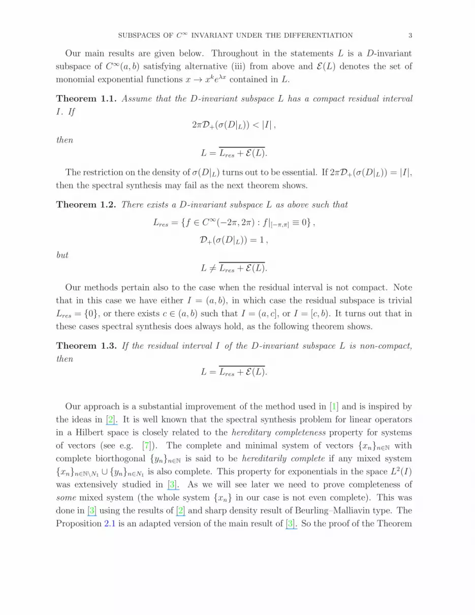
Our main results are given below. Throughout in the statements L is a D-invariant
subspace of C∞(a, b) satisfying alternative (iii) from above and E(L) denotes the set of
monomial exponential functions x→ xkeλx contained in L.
Theorem 1.1. Assume that the D-invariant subspace L has a compact residual interval
I. If
2πD+(σ(D|L)) < |I| ,then
L = Lres + E(L).
The restriction on the density of σ(D|L) turns out to be essential. If 2πD+(σ(D|L)) = |I|,then the spectral synthesis may fail as the next theorem shows.
Theorem 1.2. There exists a D-invariant subspace L as above such that
Lres = {f ∈ C∞(−2π, 2π) : f |[−π,π] ≡ 0} ,D+(σ(D|L)) = 1 ,
but
L 6= Lres + E(L).
Our methods pertain also to the case when the residual interval is not compact. Note
that in this case we have either I = (a, b), in which case the residual subspace is trivial
Lres = {0}, or there exists c ∈ (a, b) such that I = (a, c], or I = [c, b). It turns out that in
these cases spectral synthesis does always hold, as the following theorem shows.
Theorem 1.3. If the residual interval I of the D-invariant subspace L is non-compact,
then
L = Lres + E(L).
Our approach is a substantial improvement of the method used in [1] and is inspired by
the ideas in [2]. It is well known that the spectral synthesis problem for linear operators
in a Hilbert space is closely related to the hereditary completeness property for systems
of vectors (see e.g. [7]). The complete and minimal system of vectors {xn}n∈N with
complete biorthogonal {yn}n∈N is said to be hereditarily complete if any mixed system
{xn}n∈N\N1∪ {yn}n∈N1
is also complete. This property for exponentials in the space L2(I)
was extensively studied in [3]. As we will see later we need to prove completeness of
some mixed system (the whole system {xn} in our case is not even complete). This was
done in [3] using the results of [2] and sharp density result of Beurling–Malliavin type. The
Proposition 2.1 is an adapted version of the main result of [3]. So the proof of the Theorem

4 ALEXANDRU ALEMAN, ANTON BARANOV, YURII BELOV
1.1 consists of two steps: we reduce the problem to a Hilbert space problem (Section 2)
and solve the appropriate mixed completeness problem (Section 3).
The idea of the construction of the counterexample in Theorem 1.2 goes back to [2,
Theorem 1.3].
Organization of the paper. The paper is organized as follows. Theorem 1.1 is proved
in Sections 2 and 3. Example of the absence of spectral synthesis is given in Section 4. In
Section 5 we prove Theorem 1.3.
2. Proof of Theorem 1.1
2.1. Preliminaries. The continuous linear functionals on C∞(a, b) are compactly sup-
ported distributions of finite order on the interval (a, b) (that is, distributions of the form
ϕ = f (n), n ∈ N, where f ∈ L1loc(a, b) and differentiation is understood in the sense of dis-
tributions). We denote this class by S(a, b). As usual we can define the Fourier transform
of ϕ ∈ S(a, b) by the formula
ϕ(z) = ϕ(eiz).
Since ϕ has finite order, the function ϕ is an entire function of finite exponential type with
at most polynomial growth on the real line. Put
HI =
{f : f =
n∑
k=0
zk(fk(z) + ck), fk ∈ PWI , ck ∈ C
},
where PWI is the Fourier image of the space L2(I). For every functional ϕ ∈ S(a, b) we
have ϕ ∈ HI , where I = I(ϕ) is a closed interval such that suppϕ ⊂ I.
Under the Fourier transform the duality between S(a, b) and C∞(a, b) becomes the du-
ality between the space H = ∪I⊂(a,b)HI and the space of entire functions U with conjugate
indicator diagrams in (a, b) and decreasing faster than any polynomial along the real line.
Let F ∈ ∪I⊂(a,b)HI , G ∈ U . If F has infinite number of zeros, then its bilinear form
(F,G)H,U = (F , G)S(a,b),C∞(a,b) can be viewed as usual inner product in L2(R) (or PWI)
of the functions F (z)/P (z) and G(z)P (z), where P is a polynomial of a sufficiently large
degree whose zero set is a subset of zero set of F . This explains how spaces PWI come
into the picture.
For an entire function F we will denote its zeros set as ZF .
2.2. The associated a Hilbert space problem. Let us denote Λ = σ(D|L),
L0 = Lres + E(L),
and let I be the residual interval given by
Lres = LI = {f ∈ C∞(a, b) : f (k)(I) = 0 , k ≥ 0}.

SUBSPACES OF C∞ INVARIANT UNDER THE DIFFERENTIATION 5
If I reduces to one point, it is easy to see that L = C∞(a, b). Thus we shall assume
throughout that I does not reduce to a point.
Let us consider the annihilators L⊥ and L⊥0 of L and L0 respectively in the dual space
S(a, b). It is easy to see that
L⊥0 = {F : F ∈ HI , F
∣∣Λ= 0}.
It will be sufficient to prove that L⊥ is dense in L⊥0 , in the weak star topology.
Let us consider the distribution ϕ ∈ L⊥ with the maximal length of conv suppϕ. It is
clear that ϕ ∈ HI but ϕ /∈ HJ for any subinterval J ⊂ I, J 6= I. We can write
ϕ(z) = GΛ(z)E(z),
where GΛ is some canonical product corresponding to the sequence Λ) and E is some entire
function. In fact, we shall choose GΛ such that G(z)/G(z) is a quotient of two Blaschke
products. Moreover, without loss of generality we can assume that E has no multiple zeros
and E(λ) 6= 0 for λ ∈ Λ.
From [1, Proposition 3.1] we know that
GΛ(z)E(z)
z − w∈ L⊥, w ∈ ZE .
Therefore, we can further assume that GΛE ∈ PW I , otherwise we can start with the
function E(z)(z−w1)...(z−wn)
in place of E.
We argue by contradiction. Suppose that L⊥ is not dense in L⊥0 . Then there exists
an entire function T such that GΛT ∈ HI and GΛT /∈ L⊥. We fix such a function T and
number N such that GΛ(x)T (x) = O(1+ |x|N). From the Hahn–Banach Theorem we know
that there exists a non-trivial function f ∈ C∞(I) such that(GΛ(z)E(z)
z − w, f
)= 0, w ∈ ZE and (GΛT, f) 6= 0.
In order to arrive at a Hilbert space setting we assume first that GΛT ∈ PWI . In this
case both equations may be understood as usual inner products in L2(R). The general case
(GΛT grows polynomially) will be reduced to this special situation in the next subsection.
This leads to the following system of equations
(2.1)
∫R
GΛ(x)E(x)x−w
F (x)dx = 0, w ∈ ZE ,∫RGΛ(x)T (x)F (x)dx 6= 0.
The contradiction we are seeking for is given by the following proposition. The repro-
ducing kernel at λ in PWI will be denoted by kλ.

6 ALEXANDRU ALEMAN, ANTON BARANOV, YURII BELOV
Proposition 2.1. Let G ∈ PWI be a function with simple zeros and such that G /∈ PWJ
for any proper subinterval J of I. If we have a partition of its zero set ZG = Λ1 ∪ Λ2,
Λ1 ∩ Λ2 = ∅ such that 2πD+(Λ2) < |I|, then the mixed system
(2.2) {kλ}λ∈Λ2∪{G(z)
z − λ
}
λ∈Λ1
is complete in PWI .
Let us assume for the moment that Proposition 2.1 is proved, and that GΛT ∈ PWI .
From (2.1) it follows that F is orthogonal (in PWI) to the family{
GΛ(z)E(z)z−w
}w∈ZE
. Apply
Proposition 2.1 to the function G = GΛE, with Λ2 = Λ,Λ1 = ZE, to conclude that F
belongs to the closed span of {kλ}λ∈Λ, which obviously contradicts the second equation in
(2.1).
2.3. Reduction of the general case to the Hilbert space setting. In the general
case we only know that that GΛT (x) = O(1 + |x|N) on the real line. Put
M = {GΛH : GΛH ∈ PWI}.By the previous argument we have that L⊥ is dense in M , hence, it remains to prove that
M is dense in L⊥0 . Assume the contrary. Then there exists a function f ∈ C∞(a, b) such
that f ⊥M but (GΛT, f) 6= 0.
Let us fix a finite set W , W ∩ Λ = ∅, such that there exists a function g of the form∑w∈W cwe
iwt with the property that for 0 ≤ k ≤ 2N + 2, g(k) − f (k) vanishes at the
endpoints of I. Moreover, it is clear that there exists GΛF0 ∈ M such that GΛ(T + F0)
vanishes on W . Thus GΛ(T + F0) = GΛPWT1, where PW is a polynomial vanishing on W .
Obviously, (GΛPWT1, F ) 6= 0.
Now let F = f − g, and note that F (x) = O((1 + |x|)−2N); in particular, FQ ∈ L2(R),
for every polynomial Q of degree strictly less than 2N .
For every entire function U with GΛPWU ∈ PWI , we have the system
(2.3)
∫RGΛ(x)PW (x)U(x)F (x)dx = 0,
∫RGΛ(x)PW (x)T1(x)F (x)dx 6= 0.
Now fix a function U such that T1 and U have at least N + 2 common zeros and
GΛU /∈ PWJ for any proper subinterval J ⊂ I . Then write U = QU1, T1 = QT2, where
Q is a polynomial of degree N + 2 and let Q∗(z) = Q(z). We then have
(GΛPWT2, FQ∗) 6= 0,
(GΛPWU1
z − u, FQ∗
)= 0, if u ∈ ZU1
,
which is a system of the form (2.1) with the set Λ ∪W instead of Λ and with U1 instead
of E. As we have seen in the previous subsection this system leads to a contradiction. �

SUBSPACES OF C∞ INVARIANT UNDER THE DIFFERENTIATION 7
3. Proof of Proposition 2.1
In order to complete the proof of Theorem 1.1 it remains to prove Proposition 2.1. To
simplify notations we assume without loss that I = [−π, π] and write PWπ instead of
PW [−π,π]. We denote by kλ the reproducing kernel of PWπ corresponding to the point λ,
that is,
kλ(z) =sin π(z − λ)
π(z − λ), and f(λ) = (f, kλ).
Recall that for any γ ∈ R the system {kn+γ}n∈Z is an orthogonal basis of PWπ.
3.1. Equation for the function of zero exponential type. The proof is similar to
the proof of the main theorem in [2]. Assume the contrary. Then there exists a nonzero
h ∈ PWπ such that
(3.1)
(h,G(z)
z − λ
)= 0, λ ∈ Λ1, (h, kλ) = 0, λ ∈ Λ2.
We expand h with respect to the orthogonal basis {kn}n∈Z:
h(z) =∑
n
ankn(z).
Then the equations (3.1) can be rewritten as
(3.2)
∑n
anG(n)λ−n
= 0, λ ∈ Λ1,∑
n(−1)nanλ−n
= 0, λ ∈ Λ2.
Then there exist entire functions S1 and S2 such that
(3.3)
∑n
anG(n)z−n
= G1(z)S1(z)sinπz∑
n(−1)nan
z−n= G2(z)S2(z)
sinπz= h(z)
sinπz,
where G1 and G2 are canonical products corresponding to Λ1,Λ2, respectively. The func-
tions S1, S2 satisfying (3.3) parametrize all functions orthogonal to the mixed system (2.2).
Put V = S1S2. Comparing the residues in equations (3.3) at the points n we get
V (n) = (−1)n|an|2.
Therefore we have the representation
V (z) = Q(z) +R(z) sin πz,
where
Q(z) = sin πz∑
n
|an|2z − n

8 ALEXANDRU ALEMAN, ANTON BARANOV, YURII BELOV
and R is a function of zero exponential type. Without loss of generality we can assume
that S1 and S2 are real on the real line (the similar formulae hold for S1 +S∗1 and S2 +S∗
2 ,
see [2]). We know that
(3.4) R(λ) +∑
n
|an|2λ− n
= 0, λ ∈ ZS2.
This is a very restrictive condition because we can start with a basis {kn+γ}n∈Z, γ ∈ [0, 1)
which is sufficiently far from real the zeros of S2 so that the Cauchy transform of the
sequence |an|2 is not very big on real zeros of S2. On the other hand, there are a lot of real
zeros of S2 because the function V has at least one zero in each interval [n, n+ 1). In the
next subsection we present this idea in detail.
3.2. Choice of the basis. Choosing amongst the bases {kn+γ}, γ ∈ R, is of course equiv-
alent to the corresponding translation to the functions involved. For simplicity, we shall
keep the same notations for these. Then we can find a sufficiently small δ > 0 for which
there exist two subsets Σ,Σ1 of the zero set Z(S2) of the function S2 with the following
properties:
• Σ has exactly one point in those intervals where Z(S2) ∩ [n, n+ 1) 6= ∅, and
dist(x,Z) >δ
1 + x2, x ∈ Σ;
• Σ1 has positive upper density, and dist(x,Z) > δ, x ∈ Σ1.
We need to consider three cases. If R is a nonzero polynomial, then the zeros of the
function (3.4) approach Z and we obtain a contradiction to the existence of Σ1. If R = 0,
then it is known that the density of Σ1 is zero [2, Proposition 3.1]. Finally, if R is not a
polynomial, we can divide it by (z − z1)(z − z2), where z1 and z2 are two arbitrary zeros
of R, z1, z2 6∈ Σ, to get a function R1 of zero exponential type which is bounded on Σ.
Next, we obtain some information on Σ. For a discrete set X = {xn} ⊂ R we consider
its counting function nX(t) = card {n : xn ∈ [0, t)}, t ≥ 0, and nX(t) = −card {n : xn ∈(−t, 0)}, t < 0. If f is an entire function and X is the set of its real zeros (counted
according to multiplicities), then there exists a branch of the argument of f on the real
axis, which is of the form arg f(t) = πnX(t) + ψ(t), where ψ is a smooth function. Such
choice of the argument is unique up to an additive constant and in what follows we always
assume that the argument is chosen to be of this form.
Denote by u the conjugate function (the Hilbert transform) of u,
u(x) =1
πv.p.
∫
R
(1
x− t+
t
t2 + 1
)u(t)dt.

SUBSPACES OF C∞ INVARIANT UNDER THE DIFFERENTIATION 9
We use the fact that for every function f ∈ PWπ with the conjugate indicator diagram
[−π, π] and all zeros in C+, one has
(3.5) arg f = πx+ u+ c,
where u ∈ L1((1 + x2)−1dx), c ∈ R.
Indeed, the function g = e−iπzf(z) is an outer function in C+ and, hence, it can be
represented in the form elog |g|+ilog |g|. Taking into account the arguments we get (3.5).
It follows from (3.3) that GV ∈ PW2π. For any f ∈ PWπ we put
f#(z) = f(z)B−(z),
where B−(z) is a Blaschke product in C− with zero set Zf ∩ C−. The function f# has no
zeros in C− and is also in PWπ. So, we have
h# = G#2 S
#2 ∈ PWπ, G#V # ∈ PW2π.
Using these inclusions and the fact that V # has at least one zero in each interval (n, n+1)
we find an equation on the counting function of Σ. In the next subsection we will show
that this contradicts to the fact that nonconstant entire function of zero exponential type
is bounded on Σ.
Let us consider its representation V # = V0H , where the zeros of V0 are simple, interlacing
with Z and V0|Σ = 0. It is clear that arg V0 = πx+O(1). Since,
arg(G#V #) = 2πx+ u1 + c,
and
arg(G#) = πx+ u2 + c,
we conclude that
arg(H) = u3 +O(1).
Consider the equality h# = G#2 HS
#2 /H and note that
arg(S2
H
)= πnΣ − α,
where α is some nondecreasing function on R. This follows from the fact that S#2 /H
vanishes only on a subset of the real axis which contains Σ. Applying the representation
(3.5) to h#, we conclude that
(3.6) argG#2 + πnΣ(x) = πx+ u+ v + α,
where u ∈ L1((1 + x2)−1dx), v ∈ L∞(R), and α is nondecreasing.
Using the fact that the upper density of Λ2 is less than π we get an equation

10 ALEXANDRU ALEMAN, ANTON BARANOV, YURII BELOV
(3.7) πnΣ(x) = πεx+ u+ v + α1, ε > 0,
and α1 is nondecreasing.
Summing up, we have an entire function R of zero exponential type which is not a
polynomial, and which is bounded on a set Σ ⊂ R satisfying (3.7).
3.3. Beurling–Malliavin meets Polya. To deduce a contradiction from (3.7), we use
some information on the classical Polya problem and on the second Beurling–Malliavin
theorem. We say that a sequence X = {xn} ⊂ R is a Polya sequence if any entire function
of zero exponential type which is bounded on X is a constant. We say that a disjoint
sequence of intervals {In} on the real line is a long sequence of intervals if
∑
n
|In|21 + dist2(0, In)
= +∞.
A complete solution of the Polya problem was obtained by Mishko Mitkovski and Alexei
Poltoratski [9]. In particular a separated sequence X ⊂ R is not a Polya sequence if and
only if there exists a long sequence of intervals {In} such that
card(X ∩ In)|In|
→ 0.
Applying this result to our R and Σ (formally speaking, Σ is not a separated sequence
but by construction it is a union of two separated sequences which are interlacing), we find
a long system of intervals {In} such that
card(Σ ∩ In)|In|
→ 0.
Given I = [a, b], denote I− = [a, (2a+ b)/3], I+ = [(a+ 2b)/3, b],
∆∗I = inf
I+[πεx− πnΣ(x) + v]− sup
I−[πεx− πnΣ(x) + v].
Now, for a long system of intervals {In} and for some c > 0 we have
∆∗In
≥ c|In|.
Next we use a version of the second Beurling–Malliavin theorem given by N. Makarov
and A. Poltoratski in [8].
Combining Proposition 3.13 and Theorem 5.9 from [8] we get
Proposition 3.1. Suppose γ ∈ C(R). If there exists c > 0 and a long system of intervals
In such that
(3.8) ∆∗In[γ] ≥ c|In|,

SUBSPACES OF C∞ INVARIANT UNDER THE DIFFERENTIATION 11
then γ cannot be represented as α + h, where α is decreasing and h ∈ L1((1 + x2)−1dx).
If we apply this for the function πεx−πnΣ(x)+v we arrive to a contradiction. Proposition
2.1 is completely proved. �
Remark 3.2. We close this subsection with an additional explanation of the result in
Proposition 3.1. Assume that |In| = o(dist(0, In)). Let hn = hχ10In be a restriction of
function h onto interval 10In (the interval of the length 10|In| and with the same center
as In). If the inequality (3.8) holds for hn, then the Kolmogorov theorem states that there
exists c such that ∫
|hn|>A
dx
1 + x2≤ c
A
∫
R
|hn(x)|dx1 + x2
, A > 1.
Choosing A = ε|In|, ε > 0 we have
|In|21 + dist2(0, In)
≤ 3c
ε
∫
R
|hn(x)|dx1 + x2
.
Summing up over n we get the contradiction
∞ =∑
n
|In|21 + dist2(0, In)
≤ C1
∑
n
∫
R
|hn(x)|dx1 + x2
≤ C2
∫
R
|h(x)|dx1 + x2
<∞.
We refer to [8] for the details.
3.4. A reformulation in terms of an approximation result. Given a distribution
ϕ and w ∈ C which is a zero of order n of its Fourier transform ϕ, we denote by ϕw,k,
1 ≤ k ≤ n, the distributions with Fourier transforms
ϕw,k(z) =ϕ(z)
(z − w)k.
As a consequence of the proof of Theorem 1.1 we have the following result.
Corollary 3.3. Let ϕ be a compactly supported distribution, let I be the convex hull of its
support, and let Λ be a subset of the zero set of ϕ (counting multiplicities). If
D+(Λ) <|I|2π,
then every distribution ψ with support in I whose Fourier transform vanishes on Λ, lies in
the weak-star closure of the linear span of {ϕw,k : w /∈ Λ}.
12 ALEXANDRU ALEMAN, ANTON BARANOV, YURII BELOV
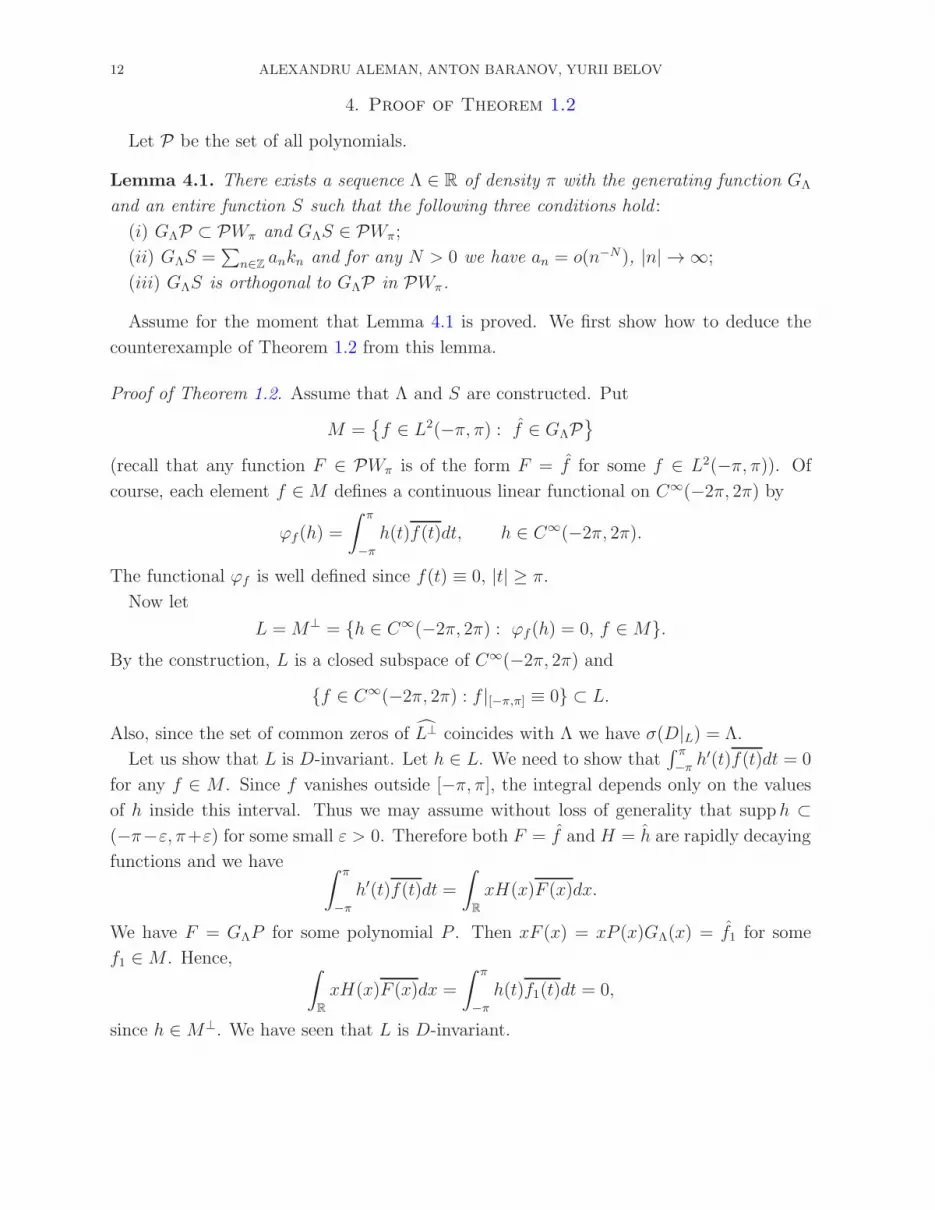
4. Proof of Theorem 1.2
Let P be the set of all polynomials.
Lemma 4.1. There exists a sequence Λ ∈ R of density π with the generating function GΛ
and an entire function S such that the following three conditions hold :
(i) GΛP ⊂ PWπ and GΛS ∈ PWπ;
(ii) GΛS =∑
n∈Z ankn and for any N > 0 we have an = o(n−N), |n| → ∞;
(iii) GΛS is orthogonal to GΛP in PWπ.
Assume for the moment that Lemma 4.1 is proved. We first show how to deduce the
counterexample of Theorem 1.2 from this lemma.
Proof of Theorem 1.2. Assume that Λ and S are constructed. Put
M ={f ∈ L2(−π, π) : f ∈ GΛP
}
(recall that any function F ∈ PWπ is of the form F = f for some f ∈ L2(−π, π)). Of
course, each element f ∈M defines a continuous linear functional on C∞(−2π, 2π) by
ϕf(h) =
∫ π
−π
h(t)f(t)dt, h ∈ C∞(−2π, 2π).
The functional ϕf is well defined since f(t) ≡ 0, |t| ≥ π.
Now let
L =M⊥ = {h ∈ C∞(−2π, 2π) : ϕf (h) = 0, f ∈M}.By the construction, L is a closed subspace of C∞(−2π, 2π) and
{f ∈ C∞(−2π, 2π) : f |[−π,π] ≡ 0} ⊂ L.
Also, since the set of common zeros of L⊥ coincides with Λ we have σ(D|L) = Λ.
Let us show that L is D-invariant. Let h ∈ L. We need to show that∫ π
−πh′(t)f(t)dt = 0
for any f ∈ M . Since f vanishes outside [−π, π], the integral depends only on the values
of h inside this interval. Thus we may assume without loss of generality that supp h ⊂(−π−ε, π+ε) for some small ε > 0. Therefore both F = f and H = h are rapidly decaying
functions and we have ∫ π
−π
h′(t)f(t)dt =
∫
R
xH(x)F (x)dx.
We have F = GΛP for some polynomial P . Then xF (x) = xP (x)GΛ(x) = f1 for some
f1 ∈M . Hence, ∫
R
xH(x)F (x)dx =
∫ π
−π
h(t)f1(t)dt = 0,
since h ∈M⊥. We have seen that L is D-invariant.

SUBSPACES OF C∞ INVARIANT UNDER THE DIFFERENTIATION 13
Now we construct a continuous functional ϕ on L such that ϕ|L0= 0, but ϕ|L 6= 0,
where, as in the proof of the first theorem,
L0 = Lres + E(L).
Let h0 ∈ L2(−π, π) be such that h0 = GΛS. Recall that GΛS =∑
n∈Z ankn where an =
o(n−N) for any N > 0. Hence, h0(t) =∑
n∈Z aneint and, by the fast decay of an we conclude
that h0 is a C∞ function in the closed interval [−π, π]. Denote by h some function in
C∞(−2π, 2π) such that h|[−π,π] = h0.
Consider the functional ϕ on L, ϕ(g) =∫ π
−πg(t)h0(t)dt. It is clear that ϕ annihilates the
set {g ∈ C∞(−2π, 2π) : g|[−π,π] ≡ 0}. Also, ϕ(eiλt) = h0(λ) = 0. Thus, ϕ annihilates L0.
Let us show that h ∈ L. Since ϕ(h) =∫ π
−π|h0(t)|2dt > 0, we then conclude that L 6= L0.
Indeed, for any f ∈M we have
ϕf (h) =
∫ π
−π
h(t)f(t)dt =
∫ π
−π
h0(t)f(t)dt
=
∫
R
h0(x)f(x)dx = 0,
since h0 = GΛS, f = GΛP for some polynomial P , and GΛS ⊥ GΛP in L2(R) by the
construction of Lemma 4.1. Thus we have constructed a functional which separates L0
and L. �
Proof of Lemma 4.1. Recall that we denote by ZF the zero set of an entire function F (all
functions involved will have simple zeros). Let
U(z) =sin(π
√z)
π√z
=∏
n∈N
(1− z
n2
),
and let V be some product with very lacunary zeros, say
V (z) =∏
n∈N
(1− z
22n + 1
).
Put
GΛ(z) =sin πz
U(z)V (z).
Note that UV tends to infinity faster than any power along R except some small neighbor-
hoods of the zeros of UV . Therefore, using, e.g., Plancherel–Polya theorem one can easily
show that GΛP ∈ PWπ for any polynomial P .
Let us introduce two more entire functions
T (z) =sin(π
√z + 1/2/10)
W (z)√z + 1/2
, W (z) =∏
n∈N
(1− z
100 · 22n − 1/2
)

14 ALEXANDRU ALEMAN, ANTON BARANOV, YURII BELOV
(note that the zeros of the nominator are exactly of the form 100n2 − 1/2, n ∈ N).
Now we define the sequence an by an := 0 for n /∈ ZU ∪ ZV and
an := (−1)nT (n), n ∈ ZU ∪ ZV .
It is easy to see that T (n) = o(n−N) for any N when n→ +∞, since sin(π√x) is bounded
for x > 0 and W (n) grows faster than any power along N.
Now we define the function S by the formula
(4.1)GΛ(z)S(z)
sin πz=
1
π
∑
n∈Z
(−1)nanz − n
.
Thus GΛS =∑
n∈Z ankn, where kn are the elements of the orthogonal basis of reproducing
kernels of PWπ (the Shannon–Kotelnikov formula), and so GΛS ∈ PWπ. This proves (i)
and (ii), since {an} has a fast decay.
Note that the summation goes only along n ∈ ZU ∪ZV , and we can rewrite (4.1) as the
following interpolation formula:
S(z)
U(z)V (z)=
1
π
∑
n∈ZU∪ZV
T (n)
z − n.
Next we put S1 = GΛT . We need to show that the following interpolation formula also
holds:S1(z)
sin πz=
1
π
∑
n∈Z
anGΛ(n)
z − n.
This formula can be rewritten in the following way using the fact that an = (−1)nT (n),
and GΛ(n) = π(−1)n((UV )′(n)
)−1, n ∈ ZU ∪ ZV :
(4.2)T (z)
U(z)V (z)=
∑
n∈ZU∪ZV
T (n)
(UV )′(n)(z − n).
We have already mentioned that T (n) decays faster than any power when n → ∞. It
is also easy to see that |(UV )′(n)| → ∞ when n → ∞ and n ∈ ZU ∪ ZV . Since V is a
lacunary product it is clear that |V (n)| is large for n ∈ ZU and |V ′(n)| is large for n ∈ ZV ,
while |U(n)|, n ∈ ZV and |U ′(n)|, n ∈ ZU , have a power-type below estimate in n. Thus,
the series in the right-hand side of (4.2) converges uniformly on compact sets separated
from the poles.
Clearly the residues coincide, and so the difference between the left and the right-hand
side of (4.2) (let us denote it byH) is an entire function. Obviously. H is of zero exponential
type. It remains to notice that the function T/(UV ) in the left-hand side tends to zero
along the imaginary axis (for the function on the right this is obvious), thus |H(iy)| → 0,
|y| → ∞, whence H ≡ 0.

SUBSPACES OF C∞ INVARIANT UNDER THE DIFFERENTIATION 15
By exactly the same arguments we may show that for any P ∈ P,
P (z)S1(z)
sin πz=
1
π
∑
n∈Z
P (n)anGΛ(n)
z − n.
It remains to verify that the function GΛS =∑
n∈Z ankn is orthogonal to all functions of
the form zkGΛ, k ∈ Z+. Let a /∈ Z and let P (z) = (z − a)zk. Since kn are the reproducing
kernels of PWπ, we have
(zkGΛ, GΛS) =1
π
∑
n∈Z
nkanGΛ(n) =1
π
∑
n∈Z
P (n)anGΛ(n)
n− a=P (z)S1(z)
sin πz
∣∣∣∣z=a
= 0.
This proves (iii) and completes the proof of the lemma. �
5. Subspaces with non-compact residual interval
In this section we prove Theorem 1.3.
We begin with a simple observation related to the absence of the residual part. Given
a distribution ϕ compactly supported on (a, b) we denote throughout this section by I(ϕ)
the convex hull of its support and by |I(ϕ)| its length. Note that if L has a residual interval
I strictly contained in (a, b) then all distributions in the annihilator of L are supported on
this interval, and clearly,
sup{|I(ϕ)| : ϕ ∈ L⊥} = |I|.the next lemma shows that this observation remains true when I = (a, b) as well.
Lemma 5.1. If σ(D|L) is an infinite discrete subset of C and Lres = {0}, thensup{|I(ϕ)| : ϕ ∈ L⊥} = b− a,
where b− a = ∞ if (a, b) has infinite length.
Proof. Let s be the supremum in the statement. Under the assumption on σ(D|L) it followseasily that s > 0. Also note that if |I(ϕ)|, |I(ψ)| > s/2, then these intervals must have a
nonempty intersection otherwise |I(ϕ+ ψ)| > s. Thus,
I =⋃
{I(ϕ) : ϕ ∈ L⊥, |I(ϕ)| > s/2}is an interval with |I| ≥ s. It is easy to see that we must have |I| = s. Indeed, if c, d ∈ I
with d − c > s such that c ∈ I(ϕ), d ∈ I(ψ), then clearly, |I(ϕ + ψ)| > s, which is a
contradiction.
We claim that I contains the interior of any interval I(ϕ), with ϕ ∈ L⊥. Assume the
contrary, i.e., that there exists ϕ ∈ L⊥ such that the interior of I(ϕ) is not contained in I.
If J is a nontrivial interval in I(ϕ) \ I, we choose ψ ∈ L⊥ with
|I(ψ)| > max{s− |J |, s/2}
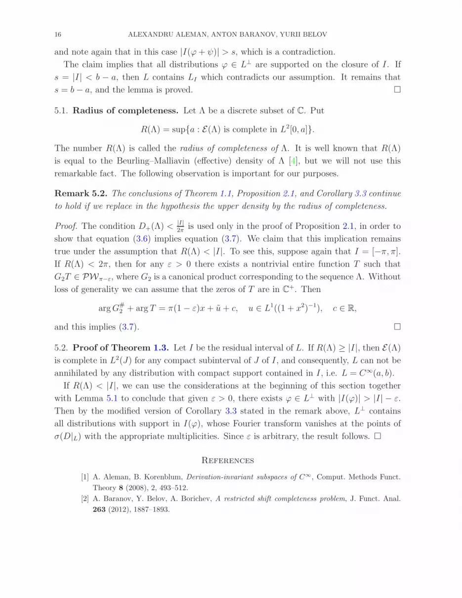
16 ALEXANDRU ALEMAN, ANTON BARANOV, YURII BELOV
and note again that in this case |I(ϕ+ ψ)| > s, which is a contradiction.
The claim implies that all distributions ϕ ∈ L⊥ are supported on the closure of I. If
s = |I| < b − a, then L contains LI which contradicts our assumption. It remains that
s = b− a, and the lemma is proved. �
5.1. Radius of completeness. Let Λ be a discrete subset of C. Put
R(Λ) = sup{a : E(Λ) is complete in L2[0, a]}.
The number R(Λ) is called the radius of completeness of Λ. It is well known that R(Λ)
is equal to the Beurling–Malliavin (effective) density of Λ [4], but we will not use this
remarkable fact. The following observation is important for our purposes.
Remark 5.2. The conclusions of Theorem 1.1, Proposition 2.1, and Corollary 3.3 continue
to hold if we replace in the hypothesis the upper density by the radius of completeness.
Proof. The condition D+(Λ) <|I|2π
is used only in the proof of Proposition 2.1, in order to
show that equation (3.6) implies equation (3.7). We claim that this implication remains
true under the assumption that R(Λ) < |I|. To see this, suppose again that I = [−π, π].If R(Λ) < 2π, then for any ε > 0 there exists a nontrivial entire function T such that
G2T ∈ PWπ−ε, where G2 is a canonical product corresponding to the sequence Λ. Without
loss of generality we can assume that the zeros of T are in C+. Then
argG#2 + arg T = π(1− ε)x+ u+ c, u ∈ L1((1 + x2)−1), c ∈ R,
and this implies (3.7). �
5.2. Proof of Theorem 1.3. Let I be the residual interval of L. If R(Λ) ≥ |I|, then E(Λ)is complete in L2(J) for any compact subinterval of J of I, and consequently, L can not be
annihilated by any distribution with compact support contained in I, i.e. L = C∞(a, b).
If R(Λ) < |I|, we can use the considerations at the beginning of this section together
with Lemma 5.1 to conclude that given ε > 0, there exists ϕ ∈ L⊥ with |I(ϕ)| > |I| − ε.
Then by the modified version of Corollary 3.3 stated in the remark above, L⊥ contains
all distributions with support in I(ϕ), whose Fourier transform vanishes at the points of
σ(D|L) with the appropriate multiplicities. Since ε is arbitrary, the result follows. �
References
[1] A. Aleman, B. Korenblum, Derivation-invariant subspaces of C∞, Comput. Methods Funct.
Theory 8 (2008), 2, 493–512.
[2] A. Baranov, Y. Belov, A. Borichev, A restricted shift completeness problem, J. Funct. Anal.
263 (2012), 1887–1893.

SUBSPACES OF C∞ INVARIANT UNDER THE DIFFERENTIATION 17
[3] A. Baranov, Y. Belov, A. Borichev, Hereditary completeness for systems of exponentials and
reproducing kernels, Adv. Math. 235 (2013), 525–554.
[4] A. Beurling and P. Malliavin, On the closure of characters and the zeros of entire functions,
Acta Math. 118 (1967), 79–93.
[5] J. Delsarte, Les fonctions moyenne-periodiques, J. Math. Pures Appl. 14 (1935), 403–453.
[6] J-P. Kahane, Sur quelques problemes d’unicite et de prolongement, relatifs aux fonctions ap-
prochables par des sommes d’exponentielles, Ann. Inst. Fourier. (Grenoble) 5 (1953–1954),
39–130.
[7] A.Markus, The problem of spectral synthesis for operators with point spectrum, Izv. Akad. Nauk
SSSR 34 (1970), 3, 662–688 (Russian); English transl.: Math. USSR-Izv. 4 (1970), 3, 670–696.
[8] N. Makarov, A. Poltoratski,Meromorphic inner functions, Toeplitz kernels, and the uncertainty
principle, in Perspectives in Analysis, Springer Verlag, Berlin, 2005, 185–252.
[9] M. Mitkovski, A. Poltoratski, Polya sequences, Toeplitz kernels and gap theorems, Adv. Math.
224 (2010), 1057–1070.
[10] L. Schwartz, Theorie generale des fonctions moyenne-periodiques, Ann. of Math. (2) 48 (1947),
857–929.
[11] L. Schwartz, Etude des sommes d’exponentielles 2nd ed. Publications de l’Institut de
Mathematique de l’Universite de Strasbourg, V. Actualites Sci. Ind., Hermann, Paris, 1959.
Alexandru Aleman,
Centre for Mathematical Sciences, Lund University,
P.O. Box 118, SE-22100 Lund, Sweden
Anton Baranov,
Department of Mathematics and Mechanics, St. Petersburg State University,
St. Petersburg, Russia,
and
National Research University Higher School of Economics,
St. Petersburg, Russia,
Yurii Belov,
Chebyshev Laboratory, St. Petersburg State University,
St. Petersburg, Russia,
j b juri [email protected]


