Embed Size (px)
Citation preview

J. Differential Equations 250 (2011) 1–25
Contents lists available at ScienceDirect
Journal of Differential Equations
www.elsevier.com/locate/jde
Darboux integrating factors: Inverse problems ✩
Colin Christopher a, Jaume Llibre b, Chara Pantazi c,∗, Sebastian Walcher d
a Department of Mathematics and Statistics, University of Plymouth, Plymouth PL2 3AJ, UKb Departament de Matemàtiques, Universitat Autònoma de Barcelona, 08193 Bellaterra, Barcelona, Spainc Departament de Matemàtica Aplicada I, Universitat Politècnica de Catalunya, EPSEB, Av. Doctor Marañón, 44-50, 08028 Barcelona, Spaind Lehrstuhl A für Mathematik, RWTH Aachen, 52056 Aachen, Germany
a r t i c l e i n f o a b s t r a c t
Article history:Received 22 July 2008Available online 23 October 2010
MSC:34C0534A3434C14
Keywords:Polynomial differential systemInvariant algebraic curveIntegrating factor
We discuss planar polynomial vector fields with prescribedDarboux integrating factors, in a nondegenerate affine geometricsetting. We establish a reduction principle which transfers theproblem to polynomial solutions of certain meromorphic linearsystems, and show that the space of vector fields with a given in-tegrating factor, modulo a subspace of explicitly known “standard”vector fields, has finite dimension. For several classes of exampleswe determine this space explicitly.
© 2010 Elsevier Inc. All rights reserved.
1. Introduction
Given a planar polynomial vector field, there is the classical problem (going back to Darboux andPoincaré) to determine an integrating factor of Darboux type, or to verify that no such factor ex-ists. The papers and survey papers by Schlomiuk [15–17] give a good introduction to this field ofresearch. A preliminary question is to determine the invariant algebraic curves of the vector field, orto ensure that no such curves exist. Several results, mostly for settings with certain additional condi-tions, are known; we mention Cerveau and Lins Neto [4], Carnicer [3], Camacho and Sad [2], Lins [11],
✩ J.L. and Ch.P. are partially supported by a MEC/FEDER grant MTM2008-03437, by a CIRIT grant number 2009SGR-410. J.L. isalso partially supported by ICREA Academia. Ch.P. is additionally partially supported by a MICINN-FEDER MTM2009-06973 andCUR-DIUE grant 2009SGR 859. C.Ch. and S.W. acknowledge the hospitality and support of the CRM and Mathematics Departmentat Universitat Autònoma de Barcelona during visits when this manuscript was prepared.
* Corresponding author.E-mail addresses: [email protected] (C. Christopher), [email protected] (J. Llibre), [email protected]
(C. Pantazi), [email protected] (S. Walcher).
0022-0396/$ – see front matter © 2010 Elsevier Inc. All rights reserved.doi:10.1016/j.jde.2010.10.013

2 C. Christopher et al. / J. Differential Equations 250 (2011) 1–25
Zoladek [21], and Esteves and Kleiman [10]. An elementary approach, which also discusses integratingfactors, is given in [20]. However, it seems that a general solution of this problem is still not withinreach. Considering and solving the corresponding inverse problems seems to be essential in order toobtain structural insight and a proper understanding of the situation. These inverse problems are nottrivial, but they are accessible.
The solution of the inverse problem for curves in the projective plane, in the case that all irre-ducible curves are smooth and all intersections transversal, has been considered by several authors.An elementary exposition is given in [7]. The nondegenerate affine setting with smooth irreduciblecurves and only transversal intersections was resolved, some years ago, using mainly tools from ele-mentary commutative algebra; see [5] and [19]. A complete solution for the general problem in theaffine plane – modulo standard tasks of algorithmic algebra – is presented in [6]. In the cited papersthe strategy was to start with a linear space of vector fields that are known to admit the given curves.Then one proceeded to show that the list is already complete, or at least that the quotient space of allvector fields admitting the curves modulo the known ones has finite dimension. The remaining finitedimensional problem is then amenable to methods of algorithmic algebra.
The inverse problem for integrating factors, which we will discuss in the present paper, seemsharder to tackle. In [13] and [5] the case of inverse polynomial integrating factors was settled if theabove-mentioned affine nondegeneracy conditions hold for the underlying curves. Moreover, in thenondegenerate projective setting the case of arbitrary exponents was resolved. Similar to the strategyfor curves, the basic approach was to obtain a sufficiently large inventory of vector fields that admita given integrating factor, and then to prove that no further ones exist.
The main theme of the present paper is a general characterization of vector fields with prescribedintegrating factors in the affine nondegenerate geometric scenario. (In other words, the underlyingprojective curves may have degenerate singular points in the projective plane as long as they arerestricted to one line.) The main result is that, modulo a subspace of ‘known’ vector fields admitting aprescribed integrating factor, only a finite dimensional problem remains. To obtain this result, we willemploy a quite simple reduction principle, which leads to a system of meromorphic linear differentialequations for functions of one variable, and more precisely to polynomial solutions of this system.Since the solution space of this meromorphic system is finite dimensional, finite dimensionality ofour quotient space follows. Moreover, one obtains a computational access to the determination of thequotient space. For several classes of examples we will prove that the dimension of the quotient spaceis zero, but we will also exhibit cases when the dimension is positive.
The remaining open problem is the degenerate affine setting; including irreducible curves withsingularities as well as non-transversal intersections. In the final section of the paper we show thatthis problem can in part be addressed by extending the space of vector fields from polynomialsto the larger class whose entries are polynomial in one variable and rational in the other. Vari-ants of the arguments from previous sections show finite dimension of the corresponding quotientspace modulo “known” vector fields, and examples illustrate that explicit results can be obtainedby computation. But transferring results back to the case of polynomial vector fields is a nontrivialproblem.
We will further investigate the degenerate affine setting in forthcoming work. In addition to con-tinuing the approach from Section 7 of this paper we will also employ sigma processes to removedegenerate singular points from the affine plane.
2. Basics and known results
We consider a complex polynomial vector field
X = P∂
∂x+ Q
∂
∂ y, (1)
on C2, sometimes also written as

C. Christopher et al. / J. Differential Equations 250 (2011) 1–25 3
X =(
PQ
),
and irreducible pairwise relatively prime polynomials f1, . . . , fr , with f := f1 · · · fr . The degree of fwill be denoted by δ( f ); the degree of X is defined here as max{δ(P ), δ(Q )}. We will also considerdegrees δx , δy with respect to the individual variables.
The question we will address in the present paper is the following: Given nonzero complex con-stants d1, . . . ,dr , under which conditions does X admit the Darboux integrating factor f −d1
1 · · · f −drr ?
It is well known (see, e.g. [7] and [5]) that the complex zero set of f (which is generally a reduciblecurve in C
2) is then invariant for the vector field; equivalently there are polynomials L1, . . . , Lr suchthat
X fi = Li · f i, 1 � i � r.
We will briefly say that in this case the vector field X admits f , or admits the curve given by f = 0. Thevector field X admits the Darboux integrating factor above if and only if
d1 · L1 + · · ·dr · Lr = div X .
The respective zero sets of f and the f i in C2 will be denoted by C and Ci . As usual, we call a point
z with f (z) = fx(z) = f y(z) = 0 a singular point of C , and analogously for the Ci . The Hamiltonianvector field of f is defined by
X f = − f y∂
∂x+ fx
∂
∂ y.
For given f , the vector fields admitting f form a linear space V f . We are interested in the struc-
ture of the subspace of V f whose elements admit the Darboux integrating factor f d11 · · · f dr
r . First, letus collect some facts and properties that are known from previous work. (See [19,7,13,5].) Clearly,vector fields of the type
X =∑
i
aif
f i· X fi + f · X (2)
with polynomials ai and a polynomial vector field X , admit f . These vector fields form a subspaceof V f which will be denoted V 1
f . Following [13], but reorganizing a little, we introduce two genericnondegeneracy conditions:
(ND1) Each Ci is nonsingular.(ND2) All singular points of C have multiplicity one (thus when two irreducible components intersect,
they intersect transversally, and no more than two irreducible components intersect at onepoint).
Note that – in contrast to [5] – there is no condition with regard to the behavior at infinity. Thefollowing result is from [7], with an improvement in [5, Theorem 3.4] (in conjunction with Theo-rem 3.6); see also [13] and [6].
Theorem 1. If the conditions (ND1) and (ND2) hold then V f = V 1f .
This is our starting point for turning to integrating factors. As above, fix complex constantsd1, . . . ,dr , all of them nonzero. The vector fields with Darboux integrating factor

4 C. Christopher et al. / J. Differential Equations 250 (2011) 1–25
(f d11 · · · f drr
)−1(3)
form a linear space F f = F f (d1, . . . ,dr), which is a subspace of V f . Let us first exhibit some of itselements; cf. [19] and [5]. Given an arbitrary polynomial g , define
Z g = Z (d1,...,dr)g
to be the Hamiltonian vector field of
g/(
f d1−11 · · · f dr−1
r
).
Lemma 2. The following statements hold.
(a) The vector field
f d11 · · · f dr
r · Z g = f · Xg −r∑
i=1
(di − 1)gf
f i· X fi (4)
is polynomial and admits the integrating factor ( f d11 · · · f dr
r )−1 . The vector fields of this type form a sub-space F 0
f = F 0f (d1, . . . ,dr) of F f (d1, . . . ,dr).
(b) Given e1, . . . , er such that every di − ei is a nonnegative integer, one has
Z (e1,...,er)g = Z (d1,...,dr)
g∗ , with g∗ := f (d1−e1)1 · · · f (dr−er)
r · g
and therefore
f (d1−e1)1 · · · f (dr−er)
r · ( f e11 · · · f er
r · Z (e1,...,er)g
) = f d11 · · · f dr
r · Z (d1,...,dr)g∗ ,
whence
f (d1−e1)1 · · · f (dr−er)
r F 0f (e1, . . . , er) ⊆ F 0
f (d1, . . . ,dr).
Proof. Obvious. �There exist vector fields in F f (1, . . . ,1) that are not in F 0
f (1, . . . ,1): For all constants αi and every
vector field X with divergence zero, the vector field
X =∑
i
αif
f i· X fi + f · X (5)
clearly admits the integrating factor f −1. More generally, if d1, . . . ,dr are all nonnegative integersthen
X = f d11 · · · f dr
r
(r∑
i=1
αi
f i· X fi + Z (d1,...,dr)
h
), (6)
with constants αi and some polynomial h, admits the integrating factor ( f d11 · · · f dr
r )−1.The following result was shown in [5]; see also Section 3 below.

C. Christopher et al. / J. Differential Equations 250 (2011) 1–25 5
Theorem 3. Suppose that conditions (ND1) and (ND2) hold, and that d1, . . . ,dr are positive integers. Then avector field X admits the integrating factor ( f d1
1 · · · f drr )−1 if and only if X is of the form (6).
The case of Darboux integrating factors that are not inverse polynomials has been resolved com-pletely in [5] when additional nondegeneracy conditions at infinity hold:
Proposition 4. Suppose that conditions (ND1) and (ND2) hold, and moreover that the homogeneous highestdegree terms of f1, . . . , fr have no multiple prime factors and are pairwise relatively prime. Then a vector fieldX admits the integrating factor (3), with some d� not a nonnegative integer, if and only if X has the form (4),thus X = f d1
1 · · · f drr · Z g for some polynomial g.
One also knows some results about degenerate settings. The following is a special case of Prop. 3.4of [19].
Proposition 5. Let f1, . . . , fr be irreducible homogeneous (thus linear) polynomials. Then a vector field Xadmits the integrating factor (3) if and only if
X = b ·(
xy
)+ f d1
1 · · · f drr · Z g
with a homogeneous polynomial b of degree∑
di − 2, and some polynomial g.
The methods employed in the proofs of Theorem 3 and Propositions 4 and 5 do not seem tobe applicable for more general settings. Our goal for the present paper is to explore the scenarioof Proposition 4 when no additional conditions at infinity are imposed. This requires different tech-niques. Achieving this goal may be a critical step since in the affine plane the nondegeneracy condi-tions (ND1) and (ND2) can be enforced by a series of sigma processes, due to a theorem by Bendixsonand Seidenberg.
3. A reduction principle
We start with an elementary observation from [5], which also was at the basis for the proofs ofTheorem 3 and Proposition 4.
Lemma 6. Let X be of the form (2), namely
X =r∑
i=1
aif
f i· X fi + f · X ∈ V 1
f
and assume that X admits the integrating factor (3), with some d� �= 1. Then
X + 1
d� − 1· f d1
1 · · · f drr · Za�
= f� · X∗,
and X∗ admits the integrating factor (f d1
1 · · · f (d�−1)� · · · f dr
r
)−1.
Therefore, modulo F 0f (d1, . . . ,dr) the vector field X is congruent to some f� · X∗ , with X∗ ∈
F f (d1, . . . ,d� − 1, . . . ,dr). Lemma 2 shows that this principle may be applied repeatedly. We cantherefore note:

6 C. Christopher et al. / J. Differential Equations 250 (2011) 1–25
Lemma 7. In order to investigate the structure of the quotient space
F (d1, . . . ,dr)/F 0f (d1, . . . ,dr)
one may replace di by 1 if di is a positive integer, and by di − ki with any positive integer ki otherwise. Inparticular we may assume that each di has real part � 1.
We use this to outline the proof of Theorem 3. By Lemma 7 one may assume d1 = · · · = dr = 1.Now step 3 of the proof of Theorem 4.2 of [5] applies. The proof in [5] also uses reduction, understronger hypotheses, which are not needed in this particular case.
In the general case, one may try to achieve degree reduction for the vector fields involved. Butwithout additional hypotheses it is impossible to keep these degrees under control when passingfrom X to X∗ in Lemma 6. Generally, such a degree reduction strategy will not work, and moreover,Proposition 5 shows that the conclusion of Proposition 4 is not always true.
But there exists a general reduction strategy which relies on a weaker principle.
Proposition 8. Given f1, . . . , fr , let n j := δy( f j) be the respective degree in y, n := ∑n j = δy( f ), and
assume that each f j = α j · yn j + · · · with nonzero constants α j , 1 � j � r.
(a) Then any vector field X ∈ V 1f which admits f = f1 · · · fr has a representation
X =r∑
i=1
aif
f i· X fi + f · ˜X
such that δy(ai) < ni for i = 1, . . . , r.(b) Assume that X admits the integrating factor (3), with some d� �= 1.
(b1) If δy(X) > n + n� − 1, then
X + 1
d� − 1· f d1
1 · · · f drr · Za�
= f� · X∗ and δy(
X∗) = δy(X) − n�.
(b2) If δy(X) � n + n� − 1, then
X + 1
d� − 1· f d1
1 · · · f drr · Za�
= f� · X∗ and δy(
X∗) � n − 1.
Proof. Given a representation
X =r∑
i=1
aif
f i· X fi + f · X,
as in (2), then whenever δy(a j) � δy( f j) one has a j = a j + b j · f j with polynomials a j and b j , andδy(a j) < n j . Substituting this in (2) and rearranging terms shows statement (a).
To prove part (b1), from (a) we have that δy(a�) < n� . Now observe
δy
(a�
f
f· X fi
)� n + n� − 2,
i

C. Christopher et al. / J. Differential Equations 250 (2011) 1–25 7
due to f i = αi yni + · · · with αi constant, and
δy( f · Xa�) � n + n� − 1.
Thus
δy(
f d11 · · · f dr
r · Za�
)� n + n� − 1.
The rest of statement (b1) and statement (b2) follows easily. �Remarks.
(i) We will always assume in the following that the two nondegeneracy conditions (ND1) and (ND2)hold.
(ii) The hypothesis on the f i can be achieved via a linear transformation of the variables, with ni =δ( f i). In this sense the principle is universally applicable, and the hypothesis will be assumedfrom now on. (Of course, one will gladly consider cases with ni < δ( f i).)
Corollary 9. When conditions (ND1) and (ND2) hold and d� is not a positive integer for some � then the ques-tion whether some vector field X ∈ F f (d1, . . . ,dr) is contained in F 0
f (d1, . . . ,dr) is reduced to the analogous
question for a vector field X ∈ F f (d1, . . . ,d� − k�, . . . ,dr) with
δy( X ) � n − 1
for some integer k� � 0.
Proof. This follows by repeated application of Proposition 8, Theorem 1, Lemma 6 and the previousremarks. �
The usefulness of the reduction principle becomes manifest next, because there is an approach tohandling vector fields of bounded y-degree:
Theorem 10. Let m1 and m2 be positive integers, and consider vector fields
X = P ∂/∂x + Q ∂/∂ y
with δy(P ) < m1 and δy(Q ) < m2 . Then the following hold:
(a) There exist vector fields
Yi = vi ∂/∂x + wi ∂/∂ y, 1 � i � s,
that are linearly independent over C[x], satisfying the degree conditions δy(vi) < m1 , δy(wi) < m2 , andall Yi admitting f , with the following property: The vector field X admits f if and only if it has a repre-sentation
X = u1(x) · Y1 + · · · + us(x) · Ys (7)
with u1, . . . , us ∈ C[x]. Moreover, the polynomials ui are uniquely determined.

8 C. Christopher et al. / J. Differential Equations 250 (2011) 1–25
(b) Assume that X is of the form (7). Given d1, . . . ,dr , there exist matrices
V (x) and B(x) = Bd1,...,dr (x)
with entries in C[x] with the following property: X is contained in F f (d1, . . . ,dr) if and only if
V (x) ·⎛⎜⎝ u′
1...
u′s
⎞⎟⎠ = B(x) ·⎛⎝ u1
...
us
⎞⎠ .
The matrices V and B have s columns and at most max{m1,m2}− 1 rows. The entries of V do not dependon d1, . . . ,dr .
Proof. (a) The vector fields of y-degree less than m1, m2 respectively in their components form a freemodule over C[x], and among these the vector fields which admit f obviously form a submodule.Since C[x] is a principal ideal domain, this submodule is also free.
(b) Let Ki, j be the cofactor of f j with respect to Yi . For X as in part (a), the cofactor of f j is thengiven by
L j =∑
i
ui · Ki, j.
Note that δy(Ki, j) � max{m1,m2} − 2. Evaluation of the integrating factor condition div X = ∑d j L j
gives
div∑
ui · Yi =∑(
ui · div Yi + Yi(ui)) =
∑(ui · div Yi) +
∑vi · u′
i =∑
d j L j,
and hence
∑i
vi · u′i =
∑i
ui
(∑j
d j · Ki, j − div Yi
). (8)
We compare coefficients of powers of y (note that only powers from 0 to max{m1,m2}−2 may occur)to obtain the assertion. �
In the following sections we will use this theorem to investigate particular geometric settings.The principal computational problem that remains is to explicitly determine the vector fields Yi . Weare able to calculate the vector fields Yi in some settings, see Sections 4, 5 and 6. But a generalconsequence for the structure of F f /F 0
f is worth noting first.
Theorem 11. Let the setting of Theorem 10 be given. If some d� is not a positive integer then
dim(
F f (d1, . . . ,dr)/F 0f (d1, . . . ,dr)
)< ∞.
Proof. Under our assumptions we can apply Proposition 8, hence we may assume the setting ofTheorem 10 with all δy(Yi) � n − 1.
We will first show that v1, . . . , vs are linearly independent over C[x]. Thus let c1, . . . , cs ∈ C[x]such that c1 v1 + · · · + cs vs = 0. Since every Yi admits f , we have

C. Christopher et al. / J. Differential Equations 250 (2011) 1–25 9
vi · fx + wi · f y = Ki · f , 1 � i � s,
with Ki the cofactor corresponding to Yi . We obtain(∑i
ci wi
)· f y =
(∑i
ci Ki
)· f .
Due to our basic assumption f and f y �= 0 are relatively prime, thus f must divide∑
ci wi . But if thissum is nonzero then it has y-degree less than n; a contradiction. So, we conclude that
∑ci wi = 0,
and therefore∑
ci Yi = 0. Since the Yi are linearly independent over C[x] we find that c1 = · · · =cs = 0.
We may now pass to C(x). In view of (8), the linear independence of v1, . . . , vs is equivalent tothe fact that the rank V = s. Thus one may choose an s × s-subsystem with invertible matrix on theleft-hand side, and obtain a meromorphic linear system⎛⎜⎝ u′
1...
u′s
⎞⎟⎠ = A(x) ·⎛⎝ u1
...
us
⎞⎠ . (9)
The space of solutions of this system has finite dimension s, and so, a fortiori, contains the subspace ofpolynomial solutions. The dimension of the latter is an upper bound for the dimension of F f /F 0
f . �In the following sections we will explicitly determine system (9) for several geometric scenarios,
and use it to determine F f /F 0f . We therefore recall some facts about meromorphic linear systems. In
Cn consider a system of linear differential equations
w ′ = A(x) · w
with the entries of A meromorphic; thus each singular point x0 is (at most) a pole, and we have aLaurent expansion
A(x) = (x − x0)−� · A−� + · · · , A−� �= 0,
with some integer � and a constant matrix A−� . If there exists a solution that is meromorphic in x0,i.e.
w(x) = (x − x0)q wq + · · · , wq �= 0,
with some integer q � 0, then substitution into the differential equation leads to
q(x − x0)q−1 · wq + · · · = (x − x0)
q−� · A−�wq + · · · .
For � > 1 we see that necessarily
A−� · wq = 0;
thus A−� admits the eigenvector wq with eigenvalue 0. For � = 1 (the case of a weak singular point)we obtain the necessary condition

10 C. Christopher et al. / J. Differential Equations 250 (2011) 1–25
A−1 · wq = q · wq,
thus A−1 admits the eigenvector wq with integer eigenvalue q. If the solution is holomorphic inx0 then q must be a nonnegative integer. There is an extensive theory for weak singular points ofmeromorphic linear systems; see for instance Ch. 4 of Coddington and Levinson [9]. In what followswe will only need the fact that the existence of meromorphic solutions at singular points of A hasimplications for the eigenvalues of A−� .
The singular point at infinity is of particular interest to us; see Coddington and Levinson [9, Ch. 4,Section 6]. To analyze this point, introduce
v = x−1; dw
dv= − 1
v2
dw
dx.
Hence
dw
dv= −v−2 A
(v−1) · w = (
v−�B−� + · · ·) · w,
and one considers the singularity of this system at v = 0. If ∞ is a weak singular point of system w ′ =A(x) · w then the eigenvalues of A∞ := B−1 are of particular significance: If a polynomial solution
w = w0 + x · w1 + · · · + xm · wm
exists for w ′ = A(x) · w then
w(v) = v−m · wm + · · · + v−1 · w1 + w0,
and the eigenvalue −m of A∞ is just the negative degree of the polynomial solution in question.
4. One irreducible factor – special curves
We will first apply the reduction principle and Theorem 10 to the case of one irreducible curve.In the present section we will focus on the special class of smooth irreducible curves defined by apolynomial
f (x, y) = ym − p(x) (10)
with m � 2 an integer and p a polynomial in one variable with no multiple roots. This class includeselliptic and hyperelliptic curves. We are interested in F f (d) for all nonzero d, and there only remainsthe case when d is not a positive integer; see Theorem 3. Due to Lemma 7 we may assume thatRe d < 1. By Corollary 9, modulo F 0
f it is sufficient to consider the problem for a vector field
Y =(
b1b2
)for some polynomials b1 and b2 of y-degree � m − 1 (and still with Re d < 1). We proceed assuggested by Theorem 10, and first determine the vector fields of this type which admit the poly-nomial f .

C. Christopher et al. / J. Differential Equations 250 (2011) 1–25 11
Lemma 12. A vector field Y = b1 ∂/∂x + b2 ∂/∂ y with δy(bi) � m − 1 for i = 1,2 admits f if and only if
Y = u0(x)Y0 + u1(x) · Y1 + · · · + um−1(x) · Ym−1
with polynomials u0, u1, . . . , um−1 in one variable, and
Y0 :=(
mym−1
p′(x)
), Y j :=
(mp(x)y j−1
p′(x)y j
)for 1 � j � m − 1.
Proof. We start from
Y = (u0(x) + u1(x)y + · · · + um−1(x)ym−1) ·
(mym−1
p′(x)
)+ (
ym − p(x)) ·
(...
).
Rewrite this expression, replacing ym+k by p · yk in the first summand and changing the secondaccordingly. This yields
u0(x) ·(
mym−1
p′)
+ u1(x) · Y1 + · · · + um−1(x) · Ym−1 + (ym − p(x)
) ·(
...
).
The last term must vanish by degree considerations, and the lemma follows. �Theorem 13. Let d be nonzero, and not a positive integer. For any polynomial f as in (10) one has F f (d) =F 0
f (d).
Proof. We may assume Re d < 1. Let Y be as in Lemma 12. Note that Y0 = X f . The vector field Y j
admits f with cofactor equal to K j := mp′(x)y j−1, 1 � j � m − 1, while
div(u j · Y j) = (mp(x)u′
j(x) + (m + j)p′(x)u j(x))
y j−1 ( j � 1),
div(u0 · Y0) = mu′0 ym−1.
Therefore the integrating factor condition
d ·m−1∑j=0
u j K j =m−1∑j=0
div(u j Y j)
is satisfied if and only if u′0 = 0 and
dmp′(x)u j(x) = mp(x)u′j(x) + (m + j)p′(x)u j(x), 1 � j � m − 1,
as follows from comparing powers of y. Thus u0 is constant.If j � 1 and u j �= 0 then last equality is equivalent to
u′j
u j= (d − 1 − j/m) · p′
p, 1 � j � m − 1.
Therefore u j is a constant multiple of a power of p, with the exponent given by the first factor onthe right-hand side. Since we assume that u j �= 0 this exponent must be a nonnegative integer, due

12 C. Christopher et al. / J. Differential Equations 250 (2011) 1–25
to the assumption on p. But this is impossible in view of Re d < 1. Hence u j = 0 for 1 � j � m − 1,and this completes the proof. �5. One irreducible factor – general cubic curves
As for the second class of examples, we consider smooth irreducible cubic curves determined (withno loss of generality) by a polynomial
f = y3 + p1(x) · y + p0(x). (11)
We imitate the strategy from the previous section. This leaves us with a vector field X that admits fand can be written in the form
X = a · X f + f · X, δy(a) � 2, δy( X) � 1.
Lemma 14. Modulo F 0f (d) it is sufficient to investigate vector fields of type Y = b1 ∂/∂x + b2 ∂/∂ y with
δy(b1) � 1 and δy(b2) � 2. Additionally, we may assume Re d < 1.
Proof. We may assume that Re d < 1 by Lemma 7 and Theorem 3, and this property persists infurther applications of Lemma 6. Due to Corollary 9 we can reduce the problem to vector fields Xwith δy(X) � 2. Additionally, from Proposition 8(a) we have
X = aX f + f X
with δy(a) < 3. So, δy( f X) = δy(X − aX f ) � 4, which shows that X = b1 ∂/∂x + b2 ∂/∂ y with
δy(b1) � 1 and δy(b2) � 1.Moreover, f d Za = f Xa − (d − 1)aX f and so we have
X = aX f + f X =(
1
d − 1f Xa − 1
d − 1f d Za
)+ f X,
and
X + 1
d − 1f d Za = f
(X + 1
d − 1Xa
).
Since δy(a) < 3 we can write a = a0(x) + a1(x)y + a2(x)y2 and obtain
Xa =( −2a2(x)y − a1(x)
a′2(x)y2 + a′
1(x)y + a′0(x)
).
Thus Xa = c1 ∂/∂x + c2 ∂/∂ y with δy(c1) � 1 and δy(c2) � 2 and X + 1d−1 Xa is as desired. �
Lemma 15. A vector field Y = b1 ∂/∂x + b2 ∂/∂ y with δy(b1) � 1 and δy(b2) � 2 admits f if and only if
Y = u1(x) · Y1 + u2(x) · Y2

C. Christopher et al. / J. Differential Equations 250 (2011) 1–25 13
with polynomials u1 , u2 in one variable and
Y1 :=(
3p0 + 2p1 yp′
0 y + p′1 y2
), Y2 :=
( −2p21 + 9p0 y
2p′0 p1 − 3p0 p′
1 − p1 p′1 y + 3p′
0 y2
).
Proof. Computing modulo f we have y3 ≡ −p1 y − p0 and y4 ≡ −p1 y2 − p0 y. Thus for suitablepolynomials ai = ai(x) we get
Y ≡ (a0 + a1 y + a2 y2) ·
(−3y2 − p1p′
1 y + p′0
)≡
((3a1 p0 − p1a0) + (2a1 p1 + 3a2 p0)y + (2a2 p1 − 3a0)y2
(p′0a0 − p′
1 p0a2) + (p′0a1 + p′
1a0 − p′1 p1a2)y + (p′
0a2 + p′1a1)y2
).
Considering degrees with respect to y one sees that Y actually must be equal to the last vector fieldin this chain of equivalences, and moreover that 3a0 = 2a2 p1. Set a1 = u1, a2 = 3u2 and rearrangeterms to obtain the assertion. �
Modulo F 0f there remains the investigation of the vector fields in Lemma 15. Following the strat-
egy suggested by Theorems 10 and 11, we obtain a meromorphic linear system.
Proposition 16. Let f be given as in (11) and assume that d is not a positive integer. The vector field Y inLemma 15 admits the integrating factor f −d, if and only if the polynomials u1 and u2 satisfy(
u′1
u′2
)= 1
�· B(x)
(u1u2
)(12)
with the discriminant � = 27p20 + 4p3
1 of f , and
B(x) =(
(3d − 4) · (9p0 p′0 + 2p2
1 p′1) (3d − 5) · (−3p1) · (3p0 p′
1 − 2p′0 p1)
(3d − 4) · (3p0 p′1 − 2p′
0 p1) (3d − 5) · (9p0 p′0 + 2p2
1 p′1)
).
Moreover, we have
dim F f (d)/F 0f (d) � 1.
Proof. The cofactors of Y1 and Y2, respectively, are
K1 = 3p′0 + 3p′
1 y,
K2 = −3p1 p′1 + 9p′
0 y
while
div Y1 = 4p′0 + 4p′
1 y,
div Y2 = −5p1 p′1 + 15p′
0 y.
Evaluating the integrating factor condition
div(u1Y1 + u2Y2) = d · (u1 K1 + u2 K2)

14 C. Christopher et al. / J. Differential Equations 250 (2011) 1–25
yields (3p0 −2p2
12p1 9p0
)·(
u′1
u′2
)=
((3d − 4)p′
0 −(3d − 5)p1 p′1
(3d − 4)p′1 (3d − 5) · 3p′
0
)·(
u1u2
)and inverting the matrix on the left-hand side we obtain the meromorphic linear system (12). There-fore dim F f (d)/F 0
f (d) � 2. We note that the diagonal elements of B(x) are (3d − 4) · �′/6 and(3d − 5) · �′/6, respectively and we may suppose that Re(d − 3/2) < 0.
Now assume that dim F f (d)/F 0f (d) = 2. Then system (12) admits a polynomial fundamental sys-
tem with polynomial Wronskian w(x), and
w ′(x) = trB(x)
�(x)· w(x)
= (d − 3/2)�′(x)
�(x)· w(x).
But this implies that d −3/2 is a nonnegative integer; a contradiction. Therefore dim F f (d)/F 0f (d) < 2
and this completes the proof. �Remark. The meromorphic linear system has obvious solutions for some special values of the expo-nent:
Y1 ∈ F f (4/3) (u1 = 1, u2 = 0),
Y2 ∈ F f (5/3) (u1 = 0, u2 = 1).
One verifies directly that Y1 is of the form (4) with g = −3y, and that Y2 is of the form (4), withg = −9/2y2 − 3p1. One may proceed to show that
F f (4/3 + k) = F 0f (4/3 + k) and F f (5/3 + k) = F 0
f (5/3 + k)
for every integer k � 0.
In order to gain a general perspective, we turn to singular points of system (12). These singularpoints are not necessarily weak singularities: First, the discriminant � may have multiple roots evenfor a smooth and irreducible curve. (One example is given by f = y3 + xy + x, with p0 = p1 = x.)Second, the upper right entry of the matrix in Proposition 16 may have degree greater than or equalto the degree of �, which implies the existence of a pole of order > 1 at infinity. (Generally, givenpolynomials r and s with leading coefficients lc(r) and lc(s), the transform of the rational functionr(x)/s(x) will be
−v−2r(
v−1)/s(
v−1) = −vδ(s)−δ(r)−2 · (lc(r)/ lc(s) + · · ·)with the dots indicating existence of terms of v of positive order.)
One may distinguish various cases here, and we discuss two of them:
(i) Assuming that 2δ(p0) > 3δ(p1) (thus δ(�) = 2δ(p0)), the upper right entry of B(x) has precisedegree 2δ(p1) + δ(p0) − 1, and this is smaller than δ(�) if and only if 2δ(p1) � δ(p0). This latercondition is necessary and sufficient for the existence of a weak singular point at infinity. (Thelower left element of B(x) causes no problem.) For instance, in the case δ(p0) = 5 and δ(p1) = 3the singular point at infinity of the system is not weak.

C. Christopher et al. / J. Differential Equations 250 (2011) 1–25 15
(ii) Assuming that 2δ(p0) < 3δ(p1) (thus δ(�) = 3δ(p1)), the upper right entry of B(x) has pre-cise degree 2δ(p1) + δ(p0) − 1, and this is smaller than δ(�) if and only if δ(p1) � δ(p0). Thislater condition is necessary and sufficient for the existence of a weak singular point at infinity.(Again, the lower left element of B(x) causes no problem.) For instance, in the case δ(p0) = 4 andδ(p1) = 3 the singular point at infinity of the system is not weak.
The remaining case 2δ(p0) = 3δ(p1) is more complicated, since one has to take cancellations ofhighest-degree terms into account.
We do not aim at a complete discussion of all cubic curves in this section, but we obtain quitedefinitive results for the cases (i) and (ii) above, assuming that there is a weak singularity at infinity.
Proposition 17. The following statements hold for the polynomial f be given in (11).
(a) If δ(p0) � 2δ(p1) then system (12) admits a first order pole at infinity, with the coefficient matrix of v−1
being equal to
A∞ =(− 3d−4
3 δ(p0) ∗0 − 3d−5
3 δ(p0)
).
Therefore, F f (d) = F 0f (d) whenever d is not a positive integer.
(b) If δ(p1) � δ(p0) (and δ(p1) > 0) then system (12) admits a first order pole at infinity, with
A∞ =(− 3d−4
2 δ(p1) ∗0 − 3d−5
2 δ(p1)
).
Therefore, F f (d) = F 0f (d) whenever d is not a positive integer.
Proof. (a) The diagonal entries of the matrix are (3d − 4)�′/(6�) and (3d − 5)�′/(6�). By our as-sumption, the degree of � is equal to 2δ(p0), the polynomial at the lower left position in the matrixof Proposition 16 has degree less than 2δ(p0) − 1 and the polynomial at the upper right has degreeno more than δ(p0) − 1. This shows the asserted form of A∞ , and in particular both eigenvalueshave positive real parts when (as we may assume) Re(d) < 1. By the eigenvalue criterion (see the endof Section 3) the system (12) has no nontrivial polynomial solutions. The proof of statement (b) isanalogous. �
Thus for large classes of cubic curves one has F f (d) = F 0f (d) for any d. It would be interesting to
know whether there exist curves and exponents with dim(F f (d)/F 0f (d)) = 1.
6. Several factors, all curves are graphs
We now consider a scenario involving several curves, with a quite simple geometric setting: Givenpolynomials p1(x), . . . , pr(x) in one variable, we let
f i := y − pi(x), 1 � i � r; f := f1 · · · fr, (13)
thus each curve Ci is the graph of some polynomial in x, and condition (ND1) is automatic. We willcontinue to assume that condition (ND2) holds. Thus for all i �= j, either p j − pi is a nonzero constantor p j − pi has no common roots with its derivative; moreover for all pairwise different i, j, k thepolynomials p j − pi and pk − pi have no common root. As the first step, we apply Proposition 8 tothe vector fields admitting a given integrating factor. Since the case of inverse polynomial integratingfactors is known from Theorem 3, we may assume that not all di are positive integers. By Lemma 7

16 C. Christopher et al. / J. Differential Equations 250 (2011) 1–25
we may furthermore assume that di = 1 or Re(di) < 1 for all i when we study the dimension ofF f (d1, . . . ,dr)/F 0
f (d1, . . . ,dr).
Lemma 18. Let f be as in (13), and let d1, . . . ,dr be given, not all of them positive integers.
(a) The vector field X lies in F f (d1, . . . ,dr) if and only if there are nonnegative integers k1, . . . ,kr , polyno-mials b1(x), . . . ,br(x) in one variable and a polynomial g such that
X = f k11 · · · f kr
r
(∑i
bi(x)f
f i· X fi
)+ f d1
1 · · · f drr · Z g,
with
X :=∑
bi(x)f
f i· X fi ∈ F f (d1 − k1, . . . ,dr − kr).
In addition, X ∈ F 0f (d1, . . . ,dr) if and only if X ∈ F 0
f (d1 − k1, . . . ,dr − kr).(b) Moreover,
X∗ =∑
i
ai(x)f
f i· X fi ∈ F f (d1, . . . ,dr)
if and only if
−∑
i
a′i · f
f i=
∑i,�: i<�
((d� − 1)ai − (di − 1)a�
) · f
f i f�· (p′
� − p′i
).
Proof. Applying Proposition 8 we obtain
X = f k11 · · · f kr
r X + f d11 · · · f dr
r Z g
and by Lemma 6 we get X ∈ F 0f (d1 − k1, . . . ,dr − kr). Additionally, from Proposition 8(a) we have
X =∑
bi(x)f
f i· X fi + f ˜X
due to δy(bi) < 1. Now applying Corollary 9 we may assume δy X < r − 1. Hence, ˜X = 0 and so X isas desired.
For part (b), note that X fi ( fk) = p′k − p′
i and X fi (ai) = −a′i . Straightforward computations show
X∗( f�) =( ∑
i: i �=�
ai · f
f i f�· (p′
� − p′i
)) · f� =: K� · f�,
div X∗ = −∑
i
a′i · f
f i+
∑i,�: i<�
(ai − a�) · f
f i f�· (p′
� − p′i
),
and the integrating factor condition follows. �

C. Christopher et al. / J. Differential Equations 250 (2011) 1–25 17
It is convenient to abbreviate
θi := di − 1, 1 � i � r (14)
for the following. We may assume Re(θi) � 0 for all i when discussing F f /F 0f . The particular incar-
nation of Theorems 10 and 11 in this section is as follows:
Theorem 19. One has
X∗ :=∑
i
ai(x)f
f i· X fi ∈ F f (d1, . . . ,dr)
if and only if the polynomials ai satisfy the meromorphic linear system
a′i =
∑j: j �=i
(θ jai − θia j) · (p j − pi)′
p j − pi. (15)
The nonzero constant solution a1 = θ1, . . . ,ar = θr of system (15) yields a scalar multiple of f d11 · · · f dr
r Z1 . Inparticular
dim(
F f /F 0f
)� r − 1.
Proof. To see necessity, start with the condition in part (b) of Lemma 18 and substitute y → pk(x)for fixed k. On the left-hand side the only nonzero term is
a′k ·
∏i �=k
(pk − pi).
On the right-hand side
f
f j f�
(x, pk(x)
) = 0 if k /∈ { j, �},
and there remains
∑�: �>k
(θ�ak − θka�)∏i �=k
(pk − pi) · (pk − p�)′
pk − p�
+∑
j: j<k
(θka j − θ jak)∏i �=k
(pk − pi) · (p j − pk)′
pk − p j
as asserted.As for sufficiency, assume that (15) holds. Then
−∑
i
a′i · f
f i=
∑i,k: i �=k
(θkai − θiak)(pk − pi)
′
pk − pi
f
f i
=∑
i,k: i<k
(θkai − θiak)(pk − pi)
′
pk − pi
(f
f i− f
fk
)
=∑
i,k: i<k
(θkai − θiak)(pk − pi)
′
pk − pi
f
f i fk( fk − f i)

18 C. Christopher et al. / J. Differential Equations 250 (2011) 1–25
and this is the assertion, in view of fk − f i = pi − pk . Finally, the solution space of (15) has dimen-sion r, and it contains a nontrivial element of F 0
f . �We proceed to investigate the constant solutions of (15) in greater detail. The multiples of the
constant solution exhibited in Theorem 19 will be called trivial constant solutions.
Proposition 20. Assume that r > 1 and Re(θi) � 0 for all i, but not all θi = 0. We define the equivalencerelation ∼ on pairs of indices by i ∼ j if and only if p j − pi is constant. Then the following hold for theconstant solutions of (15).
(a) If i and j are in different equivalence classes and θi �= 0, then a j = ai · θ j/θi is uniquely determined by ai .(b) If there are two equivalence classes I and J such that there are i ∈ I with θi �= 0, and j ∈ J with θ j �= 0
then every constant solution of (15) is trivial.(c) There exist nontrivial constant solutions of (15) if and only if there is an equivalence class I such that
|I| > 1 and θ j = 0 for all j /∈ I . In this case, the constant solutions are given by (α1, . . . ,αr) with α j = 0for all j /∈ I and αi arbitrary for i ∈ I . These correspond to the vector fields
∑i∈I
αif
f i· X fi ∈ F f (d1, . . . ,dr),
and one has
dim(
F f (d1, . . . ,dr)/F 0f (d1, . . . ,dr)
) = |I| − 1.
Proof. We first prove that θ jai −θia j = 0 whenever i and j are in different classes. To verify this, notethat
0 = a′i =
∑j
(θ jai − θia j) · (p j − pi)′
p j − pi.
If p j − pi is not constant then any root x0 of this polynomial will be a pole of (p j − pi)′/(p j − pi).
Due to condition (ND2) x0 is not a pole of any (pk − pi)′/(pk − pi) with k �= j. Therefore the identity
can hold only if all coefficients corresponding to nonconstant p j − pi vanish, and (a) is proven.Moreover, statement (b) follows easily: ai determines all ak with k /∈ I because of statement (a). In
particular a j is determined by ai . But a j in turn determines all a� with � ∈ I . Thus there is only onesolution, up to scalar multiples. A similar argument proves all but the last assertion of (c).
There remains to prove that only the trivial constant solutions of (15) lie in F 0f (d1, . . . ,dr). Thus
assume that there are constants ai and a polynomial g such that
∑ai
f
f i· X fi = f d1
1 · · · f drr · Z g .
Now from (4) consider the explicit expression
f d11 · · · f dr
r · Z g =(
− f1 · · · fr g y + g∑
i
θif
f i
)∂
∂x+
(f1 · · · fr · gx − g
∑i
θif
f ip′
i
)∂
∂ y,
and compare degrees with respect to y. Assuming g = g0(x) · ym + · · · with a nonnegative integer m,the leading term for the first entry of f d1
1 · · · f drr · Z g will be equal to
C. Christopher et al. / J. Differential Equations 250 (2011) 1–25 19
−(
m −∑
θi
)g0(x)yr+m−1 �= 0,
due to the condition on the real parts of the θi . On the other hand, the y-degree of the first entry of∑ai f / f i · X fi is at most equal to r − 1. Therefore g = g0(x), and comparing y-degrees of the second
entries shows that g is constant. Thus the remaining assertion in (c) is proven. �Remark. It is worth looking at the particular case when all p j − pi are constant; thus (15) has onlyconstant solutions. Up to an automorphism of the affine plane (given by x → x and y → y − p1(x)) wemay assume that all pi are constant. Thus the curves are just parallel straight lines, there are no singu-lar points in the affine plane, and there is only one (albeit quite degenerate) singular point at infinity.Due to Proposition 20(c) the corresponding vector fields are precisely those of the form q(y) ∂/∂xwith δ(q) < r. Given the hypotheses of Proposition 20, one has F f (d1, . . . ,dr) �= F 0
f (d1, . . . ,dr) for allr � 2. Moreover, it is easy to construct vector fields that are not integrable in an elementary man-ner, by adding suitable vector fields of the form f d1
1 · · · f drr · Z g ; see Prelle and Singer [14], and also
Singer [18].
From now on we assume that some p j − pi is not constant. We turn to analyzing the singularpoints of system (15). As it turns out, this system admits only weak singularities on the complexprojective plane.
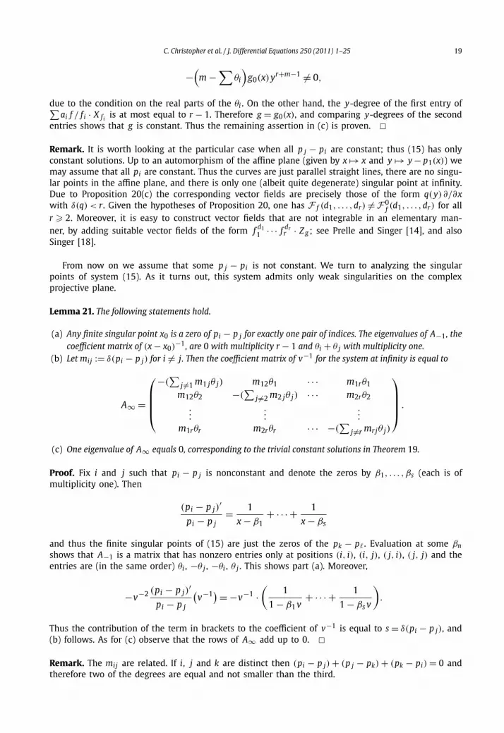
Lemma 21. The following statements hold.
(a) Any finite singular point x0 is a zero of pi − p j for exactly one pair of indices. The eigenvalues of A−1 , thecoefficient matrix of (x − x0)
−1 , are 0 with multiplicity r − 1 and θi + θ j with multiplicity one.(b) Let mij := δ(pi − p j) for i �= j. Then the coefficient matrix of v−1 for the system at infinity is equal to
A∞ =
⎛⎜⎜⎜⎝−(
∑j �=1 m1 jθ j) m12θ1 · · · m1rθ1
m12θ2 −(∑
j �=2 m2 jθ j) · · · m2rθ2
......
...
m1rθr m2rθr · · · −(∑
j �=r mrjθ j)
⎞⎟⎟⎟⎠ .
(c) One eigenvalue of A∞ equals 0, corresponding to the trivial constant solutions in Theorem 19.
Proof. Fix i and j such that pi − p j is nonconstant and denote the zeros by β1, . . . , βs (each is ofmultiplicity one). Then
(pi − p j)′
pi − p j= 1
x − β1+ · · · + 1
x − βs
and thus the finite singular points of (15) are just the zeros of the pk − p� . Evaluation at some βnshows that A−1 is a matrix that has nonzero entries only at positions (i, i), (i, j), ( j, i), ( j, j) and theentries are (in the same order) θi , −θ j , −θi , θ j . This shows part (a). Moreover,
−v−2 (pi − p j)′
pi − p j
(v−1) = −v−1 ·
(1
1 − β1 v+ · · · + 1
1 − βs v
).
Thus the contribution of the term in brackets to the coefficient of v−1 is equal to s = δ(pi − p j), and(b) follows. As for (c) observe that the rows of A∞ add up to 0. �Remark. The mij are related. If i, j and k are distinct then (pi − p j) + (p j − pk) + (pk − pi) = 0 andtherefore two of the degrees are equal and not smaller than the third.
20 C. Christopher et al. / J. Differential Equations 250 (2011) 1–25
A natural application of Lemma 21 is to investigate the dimension of F f /F 0f . Sufficient information
on the eigenvalues of A∞ can be obtained in many cases.
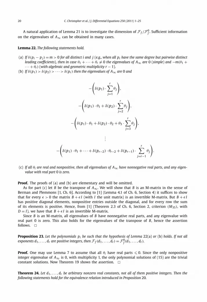
Lemma 22. The following statements hold.
(a) If δ(pi − p j) = m > 0 for all distinct i and j (e.g., when all pi have the same degree but pairwise distinctleading coefficients), then in case θ1 + · · · + θr �= 0 the eigenvalues of A∞ are 0 (simple) and −m(θ1 +· · · + θr) (with algebraic and geometric multiplicity r − 1).
(b) If δ(p1) > δ(p2) > · · · > δ(pr) then the eigenvalues of A∞ are 0 and
−(
δ(p1) ·r∑
j=1
θ j
),
−(
δ(p1) · θ1 + δ(p2) ·r∑
j=2
θ j
),
−(
δ(p1) · θ1 + δ(p2) · θ2 + θ3 ·r∑
j=3
θ j
),
...
−(
δ(p1) · θ1 + · · · + δ(pr−2) · θr−2 + δ(pr−1) ·r∑
j=r−1
θ j
).
(c) If all θi are real and nonpositive, then all eigenvalues of A∞ have nonnegative real parts, and any eigen-value with real part 0 is zero.
Proof. The proofs of (a) and (b) are elementary and will be omitted.As for part (c) let B be the transpose of A∞ . We will show that B is an M-matrix in the sense of
Berman and Plemmons [1, Ch. 6]. According to [1] (Lemma 4.1 of Ch. 6, Section 4) it suffices to showthat for every ε > 0 the matrix B + ε I (with I the unit matrix) is an invertible M-matrix. But B + ε Ihas positive diagonal elements, nonpositive entries outside the diagonal, and for every row the sumof its elements is positive. Hence, from [1] (Theorem 2.3 of Ch. 6, Section 2, criterion (M35), withD = I), we have that B + ε I is an invertible M-matrix.
Since B is an M-matrix, all eigenvalues of B have nonnegative real parts, and any eigenvalue withreal part 0 is zero. This also holds for the eigenvalues of the transpose of B , hence the assertionfollows. �Proposition 23. Let the polynomials pi be such that the hypothesis of Lemma 22(a) or (b) holds. If not allexponents d1, . . . ,dr are positive integers, then F f (d1, . . . ,dr) = F 0
f (d1, . . . ,dr).
Proof. One may use Lemma 7 to assume that all θi have real parts � 0. Since the only nonpositiveinteger eigenvalue of A∞ is 0, with multiplicity 1, the only polynomial solutions of (15) are the trivialconstant solutions. Now Theorem 19 shows the assertion. �Theorem 24. Let d1, . . . ,dr be arbitrary nonzero real constants, not all of them positive integers. Then thefollowing statements hold for the equivalence relation introduced in Proposition 20.

C. Christopher et al. / J. Differential Equations 250 (2011) 1–25 21
(a) If every equivalence class contains just one element, then
F f (d1, . . . ,dr) = F 0f (d1, . . . ,dr).
(b) If for every equivalence class I with |I| > 1 there exists an index j /∈ I such that d j is not a positive integer,then
F f (d1, . . . ,dr) = F 0f (d1, . . . ,dr).
(c) If there exists an equivalence class I with |I| > 1 such that d j is a positive integer for every j /∈ I then
F f (d1, . . . ,dr) �= F 0f (d1, . . . ,dr).
The elements of F f (d1, . . . ,dr) have the explicit form
∏i∈I
f (ei−1)
i
∏j /∈I
f(d j−1)
j ·(∑
i∈I
αif
f iX fi
)+ f d1
1 · · · f drr · Z g
with integers ei � 1, constants αi and some polynomial g.
Proof. We may assume that all θi � 0, due to Lemma 7. Then Lemma 22 shows that the only non-positive integer eigenvalue of A∞ is 0 (possibly with multiplicity > 1). Therefore, every polynomialsolution of (15) is constant, and the assertion follows with Theorem 19 and Proposition 20. �
It seems likely that the conclusion of Theorem 24 is always true, not only for real exponents.To prove this, one would need more precise information about the eigenvalues of A∞ . In any case,even allowing degeneracies for the geometric setting at infinity, one still obtains F f (d1, . . . ,dr) =F 0
f (d1, . . . ,dr) in most scenarios. It seems reasonable to conjecture that F f �= F 0f will always be an
exceptional case.
7. Degenerate geometric settings
In this final section we briefly discuss the setting when the geometric nondegeneracy conditions(ND1) and (ND2) no longer hold. We will only assume from now on that the curves f i = 0 areirreducible and pairwise relatively prime.
As it turns out, variants of the results from the previous sections continue to hold in this moregeneral context if we consider the space of vector fields that are polynomial in y and rational in x.Letting f = yn + · · · = f1 · · · fr be a polynomial as before, and given nonzero constants di , we nowconsider the subspaces
F ∗f (d1, . . . ,dr) and F ∗
f0(d1, . . . ,dr)
of this linear space. The former subspace consists of all vector fields admitting the integrating fac-tor (3), while the latter consists of all vector fields of the special form
f d11 · · · f dr
r · Z g
with g ∈ C(x)[y]. Mutatis mutandis, Lemma 2 obviously holds for these vector fields.Our starting point, in lieu of Theorem 1, is now as follows:

22 C. Christopher et al. / J. Differential Equations 250 (2011) 1–25
Lemma 25. If a polynomial vector field X admits f then
X =∑
i
aif
f i· X fi + f · X, (16)
where the ai lie in C(x)[y], and X is rational in x and polynomial in y. More precisely, there is h ∈ C[x],depending only on f , such that all ai can be chosen in C[x, y][ 1
h ].
Proof. The proof follows essentially from Theorem 6.12 of [8]. (See also [5, Theorem 3.4].) In thistheorem it was shown that for any polynomial vector field admitting f , and for every element h of acertain ideal I defined via f , there exist polynomials ai and a polynomial vector field X such that
h · X =∑
i
aif
f i· X fi + f · X .
By definition the ideal I contains the polynomials
f ,f
f i· f iy (1 � i � n)
(see [8] or [5]) which do not have a common factor in view of f = yn + · · · . Hence the zero set of I
is finite, and there exists a polynomial h(x) ∈ I ∩ C[x]. �Now Lemmas 6 and 7, Proposition 8 and Corollary 9 carry over to the present setting with obvious
modifications. (In order to apply Lemma 25, one may have to multiply by powers of h, but this isharmless.) If all di are positive integers then we end up with the case d1 = · · · = dr = 1, for which[5, Proposition 4.3] shows that
X =∑
i
βif
f i· X fi + f · Xg (17)
with constants βi and some rational function g . (This may be seen as a counterpart to Theorem 3.)For the remaining exponents we can reduce to the case of vector fields X with δy(X) � n − 1.
Theorem 26. If some d� is not a positive integer then
dim(
F ∗f (d1, . . . ,dr)/F ∗
f0(d1, . . . ,dr)
)� n − 1.
Proof. Let X ∈ F ∗f (d1, . . . ,dr), and δy(X) � n − 1 with no loss of generality.
We start with some preliminary considerations. Let K ⊇ C(x) denote a splitting field of f ∈C(x)[y]; thus we have
f = (y − q1(x)
) · · · (y − qn(x)) =: g1 · · · gn
over K, with algebraic functions q1, . . . ,qn . Since f has no multiple prime factors over C(x), and weare in characteristic zero, the qi are pairwise distinct, whence f /g1, . . . , f /gn are relatively prime. ByLagrange interpolation, every s ∈ K[y] with degree � n − 1 has a unique representation
s =∑
ci · f
gi
i
C. Christopher et al. / J. Differential Equations 250 (2011) 1–25 23
with ci ∈ K. We note that
Xgi =( −1
−q′i(x)
)and so the vector field X can be written in the form
X =∑
i
ai(x)f
gi· Xgi +
∑i
bi(x)f
gi
∂
∂ y. (18)
If X admits f then X(gk) is a multiple of gk for each k, thus
0 = X(gk)(qk) =∑
i
bi(x)f
gi(qk) = bk(x)
f
gk(qk)
and therefore bk = 0. So from (18) we obtain
X =∑
i
ai(x)f
gi· Xgi (19)
similar to the setting of Lemma 18 and Theorem 19. Now an imitation of the proof of Theorem 19shows that the ai satisfy the differential equation
a′i =
∑j: j �=i
(θ jai − θia j) · (q j − qi)′
q j − qi, (20)
analogous to Eq. (15). Here θi + 1 equals the exponent of the factor f� of f which is divided by gi .As in Theorem 19, the nonzero constant solution ai = θi (1 � i � n) yields a scalar multiple off d11 · · · f dr
r Z1 ∈ F ∗f
0. In summary, the dimension of the quotient space is bounded by n − 1. �For the case of polynomial vector fields, which is of principal interest to us, this theorem provides a
strong structural result, but some questions remain open. One problem in this approach is to identifythe polynomial vector fields in F ∗
f0(d1, . . . ,dr); another problem is to utilize the differential equation
(20) beyond dimension estimates. Our final result illustrates that the differential equation can beuseful for finding vector fields in some cases. We consider the case of a “degenerate hyperellipticcurve” (compare Theorem 13 with m = 2).
Proposition 27. For f = y2 − p(x) the dimension of F ∗f (d)/F ∗
f0(d) is at most 1. Furthermore, if d is not a
positive integer then the most general first integral and X ∈ F ∗f (d) with δy(X) = n −1 is the sum of a Darboux
function and a term of the form∫ y/
√p(Z 2 − 1)−d dZ .
Proof. It is straightforward to work back through the reduction process to show that the first integralof the original system is of a similar form. The first part is just Theorem 26 if d is not a positiveinteger, and a consequence of [5, Proposition 4.3] otherwise. For the second part we use that X has arepresentation (19), and from (20) we obtain
a′1 = (d − 1)(a1 − a2)
p′, a′
2 = (d − 1)(a2 − a1)p′
,
2p 2p
24 C. Christopher et al. / J. Differential Equations 250 (2011) 1–25
noting q1 = √p = −q2. Thus a1 + a2 is a constant, which we may take to be 0 in view of the last
argument in the proof of Theorem 26. There remains
a′1 = 2(d − 1)a1
p′
ph,
which gives
a1 = �pd−1, a2 = −�pd−1
for some constant �. Going back to (19), we find
1
(y2 − p(x))d· X = �pd−1
(y2 − p(x))d−1· Xw (21)
with
w := ln
(y − √
p
y + √p
).
This vector field admits the first integral
�
2
y/√
p∫dZ
(Z 2 − 1)d. �
We note that this candidate for an exceptional vector field can only work when pd−1 is a rationalfunction.
8. Note added in proof
The assertion of Theorem 11 holds in general, even if assumptions (ND1) and (ND2) are not satis-fied. This is shown in a forthcoming paper [12], using properties of σ -processes. But as it turns out,the essential part of the finiteness proof is contained in Section 3 of the present paper.
References
[1] A. Berman, R.J. Plemmons, Nonnegative Matrices in the Mathematical Sciences, SIAM, Philadelphia, 1994.[2] C. Camacho, P. Sad, Invariant varieties through singularities of holomorphic vector fields, Ann. Math. 15 (1982) 579–595.[3] M. Carnicer, The Poincaré problem in the nondicritical case, Ann. Math. 140 (1994) 289–294.[4] D. Cerveau, A. Lins Neto, Holomorphic foliations in CP(2) having an invariant algebraic curve, Ann. Inst. Fourier 41 (1991)
883–903.[5] C. Christopher, J. Llibre, Ch. Pantazi, S. Walcher, Inverse problems for multiple invariant curves, Proc. Roy. Soc. Edinburgh
Sect. A 137 (2007) 1197–1226.[6] C. Christopher, J. Llibre, Ch. Pantazi, S. Walcher, Inverse problems for invariant algebraic curves: explicit computations, Proc.
Roy. Soc. Edinburgh Sect. A 139 (2009) 287–302.[7] C. Christopher, J. Llibre, Ch. Pantazi, X. Zhang, Darboux integrability and invariant algebraic curves for planar polynomial
systems, J. Phys. A 35 (2002) 2457–2476.[8] C. Christopher, J. Llibre, J.V. Pereira, Multiplicity of invariant algebraic curves in polynomial vector fields, Pacific J.
Math. 229 (1) (2007) 63–117.[9] E.A. Coddington, N. Levinson, Theory of Ordinary Differential Equations, McGraw–Hill, New York, 1955.
[10] E. Esteves, S. Kleiman, Bounds on leaves of one-dimensional foliations, Bull. Braz. Math. Soc. (N.S.) 34 (2003) 145–169.[11] A. Lins Neto, Algebraic solutions of polynomial differential equations and foliations in dimension two, in: Holomorphic
Dynamics, in: Lecture Notes in Math., vol. 1345, Springer-Verlag, Berlin/New York, 1988, pp. 192–232.[12] J. Llibre, C. Pantazi, S. Walcher, Morphisms and inverse problems for Darboux integrating factors, preprint, 2009.

C. Christopher et al. / J. Differential Equations 250 (2011) 1–25 25
[13] Ch. Pantazi, Inverse problems of the Darboux theory of integrability for planar polynomial differential systems, Doctoralthesis, Universitat Autonoma de Barcelona, 2004.
[14] M.J. Prelle, M.F. Singer, Elementary first integrals of differential equations, Trans. Amer. Math. Soc. 279 (1983) 613–636.[15] D. Schlomiuk, Algebraic particular integrals, integrability and the problem of the center, Trans. Amer. Math. Soc. 338 (1993)
799–841.[16] D. Schlomiuk, Elementary first integrals and algebraic invariant curves of differential equations, Expo. Math. 11 (1993)
433–454.[17] D. Schlomiuk, Algebraic and geometric aspects of the theory of polynomial vector fields, in: D. Schlomiuk (Ed.), Bifurcations,
Periodic Orbits of Vector Fields, Kluwer Academic Publishers, Dordrecht, 1993, pp. 429–467.[18] M.F. Singer, Liouvillian first integrals of differential equations, Trans. Amer. Math. Soc. 333 (1992) 673–688.[19] S. Walcher, Plane polynomial vector fields with prescribed invariant curves, Proc. Roy. Soc. Edinburgh Sect. A 130 (2000)
633–649.[20] S. Walcher, On the Poincaré problem, J. Differential Equations 166 (2000) 51–78.[21] H. Zoladek, On algebraic solutions of algebraic Pfaff equations, Studia Math. 114 (1995) 117–126.


