Embed Size (px)
Citation preview

Data Dissemination for Distributed Computing
A DISSERTATION
SUBMITTED TO THE FACULTY OF THE GRADUATE SCHOOL
OF THE UNIVERSITY OF MINNESOTA
BY
Jinoh Kim
IN PARTIAL FULFILLMENT OF THE REQUIREMENTS
FOR THE DEGREE OF
Doctor Of Philosophy
Prof. Jon B. Weissman, Co-Advisor
Prof. Abhishek Chandra, Co-Advisor
February, 2010

c⃝ Jinoh Kim 2010
ALL RIGHTS RESERVED

Acknowledgements
Some of the materials in this thesis originally came from published papers: the accessi-
bility estimation work is from ICDCS and TPDS publications [1, 2] and the collective
data access work was published in CCGrid [3]. The OPEN work and parallel data ac-
cess are currently under submission. Many individuals have helped me over past several
years, as well as they have for this thesis, and I would like to acknowledge their contri-
butions here. Bret McGuire provided me his code for PlanetLab experiments. I would
like to thank Seonho Kim for his help in getting me started. I would also like to thank
Saurabh Jain for his kind suggestions and for listening to me as I pursued my work. In
addition, I would like to acknowledge Mike Cardosa for his invaluable feedback. I am
grateful, moreover, to Siddharth Ramakrishnan, Atul Katiyar, and Robert Reutiman
for their many suggestions. I would additionally like to thank the other members of
DCS for their kindness and suggestions.
In particular, I would especially like to thank my advisers, Jon Weissman and Ab-
hishek Chandra, for their generosity, patience, and guidance. I am very grateful for
the chance to have worked with them. I also deeply appreciate Zhi-Li Zhang for his
theoretical help and David Lilja for his advanced insights.
Lastly, I would like to thank my lovely family, Myunghwa, Minsoo, and Aujin, for
their love and support. I would also like to give thanks to our parents, sisters, and
brothers, for their encouragement and understanding. Many thanks to the CS Korean
fellows, Myunghwan Park, Hunjeong Kang, Dongchul Park, and Taehyun Hwang. A spe-
cial thanks to Ikkyun Kim, Sangman Lee, Heesook Choi, Chunglae Cho, and Jungchan
Na. I would like to extend my appreciation to Seogjoo Hwang, Sekwon Jang, Kyo Suh,
Sungjun Jo, Chulmin Kang, and all of the members at the KPCM Paul Mission.
i

Dedication
Dedicated to my love Myunghwa,
my sweetheart Minsoo and Aujin,
and our parents.
ii

Data Dissemination for Distributed Computing
by Jinoh Kim
ABSTRACT
Large-scale distributed systems provide an attractive scalable infrastructure for net-
work applications. However, the loosely-coupled nature of this environment can make
data access unpredictable, and in the limit, unavailable. This thesis strives to provide
predictability in data access for data-intensive computing in large-scale computational
infrastructures.
A key requirement for achieving predictability in data access is the ability to estimate
network performance for data transfer so that computation tasks can take advantage
of the estimation in their deployment or data source selection. This thesis develops
a framework called OPEN (Overlay Passive Estimation of Network Performance) for
scalable network performance estimation. OPEN provides an estimation of end-to-end
accessibility for applications by utilizing past measurements without the use of explicit
probing. Unlike existing passive approaches, OPEN is not restricted to pairwise or
a single network in utilizing historical information; instead, it shares measurements
between nodes without any restrictions. As a result, it achieves n2 estimations by O(n)
measurements.
In addition, this thesis considers data dissemination in two specific environments.
First, we consider a parallel data access environment in which multiple replicated servers
can be utilized to download a single data file in parallel. To improve both performance
and fault tolerance, we present a new parallel data retrieval algorithm and explore a
broad set of resource selection heuristics. Second, we consider collective data access
in applications for which group performance is more important than individual per-
formance. In this work, we employ communication makespan as a group performance
metric and propose server selection heuristics to maximize collective performance.
iii

Contents
Acknowledgements i
Dedication ii
Abstract iii
List of Tables viii
List of Figures ix
1 Introduction 1
1.1 Contributions . . . . . . . . . . . . . . . . . . . . . . . . . . . . . . . . . 3
1.2 Dissertation Overview . . . . . . . . . . . . . . . . . . . . . . . . . . . . 4
2 Background 6
2.1 Distributed Computing Model . . . . . . . . . . . . . . . . . . . . . . . . 6
2.1.1 Replica Selection . . . . . . . . . . . . . . . . . . . . . . . . . . . 8
2.1.2 Resource Selection . . . . . . . . . . . . . . . . . . . . . . . . . . 9
2.2 Related Work . . . . . . . . . . . . . . . . . . . . . . . . . . . . . . . . . 10
2.2.1 Data Transfer Protocols . . . . . . . . . . . . . . . . . . . . . . . 10
2.2.2 Communication Performance Metrics . . . . . . . . . . . . . . . . 11
2.2.3 Server Selection . . . . . . . . . . . . . . . . . . . . . . . . . . . . 11
2.2.4 Resource Management and Discovery . . . . . . . . . . . . . . . 13
2.2.5 Network Performance Estimation . . . . . . . . . . . . . . . . . . 15
2.2.6 Probabilistic Information Dissemination . . . . . . . . . . . . . . 16
iv

2.2.7 Data Grids . . . . . . . . . . . . . . . . . . . . . . . . . . . . . . 19
2.3 Notation . . . . . . . . . . . . . . . . . . . . . . . . . . . . . . . . . . . . 19
3 Passive Data Accessibility Estimation 21
3.1 Introduction . . . . . . . . . . . . . . . . . . . . . . . . . . . . . . . . . . 21
3.2 Accessibility Estimation . . . . . . . . . . . . . . . . . . . . . . . . . . . 22
3.2.1 Accessibility Metric . . . . . . . . . . . . . . . . . . . . . . . . . 22
3.2.2 Accessibility Parameters . . . . . . . . . . . . . . . . . . . . . . . 23
3.2.3 Self-Estimation . . . . . . . . . . . . . . . . . . . . . . . . . . . . 25
3.2.4 Neighbor Estimation . . . . . . . . . . . . . . . . . . . . . . . . . 28
3.2.5 Inferring Server Latency without Active Probing . . . . . . . . . 32
3.3 Performance Evaluation . . . . . . . . . . . . . . . . . . . . . . . . . . . 35
3.3.1 Experimental Setup . . . . . . . . . . . . . . . . . . . . . . . . . 35
3.3.2 Performance Comparison over Time . . . . . . . . . . . . . . . . 37
3.3.3 Impact of Candidate Size . . . . . . . . . . . . . . . . . . . . . . 39
3.3.4 Impact of Neighbor Size . . . . . . . . . . . . . . . . . . . . . . . 39
3.3.5 Impact of Data Size . . . . . . . . . . . . . . . . . . . . . . . . . 41
3.3.6 Timeliness . . . . . . . . . . . . . . . . . . . . . . . . . . . . . . . 42
3.3.7 Multi-object Access . . . . . . . . . . . . . . . . . . . . . . . . . 43
3.3.8 Impact of Churn . . . . . . . . . . . . . . . . . . . . . . . . . . . 44
3.3.9 Impact of Replication . . . . . . . . . . . . . . . . . . . . . . . . 45
3.4 Summary . . . . . . . . . . . . . . . . . . . . . . . . . . . . . . . . . . . 48
4 OPEN: A Framework for Accessibility Estimation 51
4.1 Introduction . . . . . . . . . . . . . . . . . . . . . . . . . . . . . . . . . . 51
4.2 Secondhand Estimation . . . . . . . . . . . . . . . . . . . . . . . . . . . 53
4.2.1 Why Secondhand Estimation? . . . . . . . . . . . . . . . . . . . 54
4.3 The OPEN Framework . . . . . . . . . . . . . . . . . . . . . . . . . . . . 56
4.3.1 End-to-End Accessibility . . . . . . . . . . . . . . . . . . . . . . 56
4.3.2 Passive Estimation . . . . . . . . . . . . . . . . . . . . . . . . . . 57
4.3.3 Proactive Dissemination . . . . . . . . . . . . . . . . . . . . . . . 60
4.4 Evaluation . . . . . . . . . . . . . . . . . . . . . . . . . . . . . . . . . . . 65
4.4.1 Evaluation Methodology . . . . . . . . . . . . . . . . . . . . . . . 65
v

4.4.2 Selection Performance . . . . . . . . . . . . . . . . . . . . . . . . 66
4.4.3 Overhead Optimization . . . . . . . . . . . . . . . . . . . . . . . 72
4.4.4 Simulation with S3 Data Sets . . . . . . . . . . . . . . . . . . . . 76
4.4.5 Running Montage in the OPEN Framework . . . . . . . . . . . . 78
4.4.6 Discussion . . . . . . . . . . . . . . . . . . . . . . . . . . . . . . . 82
4.5 Summary . . . . . . . . . . . . . . . . . . . . . . . . . . . . . . . . . . . 83
5 Parallel Data Access 84
5.1 Introduction . . . . . . . . . . . . . . . . . . . . . . . . . . . . . . . . . . 84
5.2 Data Retrieval Algorithm . . . . . . . . . . . . . . . . . . . . . . . . . . 84
5.3 Resource Selection Heuristics . . . . . . . . . . . . . . . . . . . . . . . . 87
5.3.1 Latency-based Heuristics . . . . . . . . . . . . . . . . . . . . . . 88
5.3.2 Heuristics with Historical Information . . . . . . . . . . . . . . . 89
5.4 Evaluation . . . . . . . . . . . . . . . . . . . . . . . . . . . . . . . . . . . 90
5.4.1 Evaluation Methodology . . . . . . . . . . . . . . . . . . . . . . . 90
5.4.2 Simulation Results . . . . . . . . . . . . . . . . . . . . . . . . . . 90
5.5 Summary . . . . . . . . . . . . . . . . . . . . . . . . . . . . . . . . . . . 92
6 Collective Data Access 94
6.1 Introduction . . . . . . . . . . . . . . . . . . . . . . . . . . . . . . . . . . 94
6.2 Communication Makespan . . . . . . . . . . . . . . . . . . . . . . . . . . 96
6.3 Server Selection Heuristics . . . . . . . . . . . . . . . . . . . . . . . . . . 98
6.4 Performance Evaluation . . . . . . . . . . . . . . . . . . . . . . . . . . . 102
6.4.1 Experimental Testbed and Methodology . . . . . . . . . . . . . . 102
6.4.2 Comparison of Server Selection Heuristics . . . . . . . . . . . . . 104
6.4.3 Impact of Data Size . . . . . . . . . . . . . . . . . . . . . . . . . 108
6.4.4 Impact of Concurrency . . . . . . . . . . . . . . . . . . . . . . . . 110
6.5 Summary . . . . . . . . . . . . . . . . . . . . . . . . . . . . . . . . . . . 111
7 Conclusion and Future Directions 112
7.1 Conclusion . . . . . . . . . . . . . . . . . . . . . . . . . . . . . . . . . . 112
7.2 Future Directions . . . . . . . . . . . . . . . . . . . . . . . . . . . . . . . 114
7.2.1 Supporting Cluster-structured Grids . . . . . . . . . . . . . . . . 114
vi

7.2.2 Improving Estimation Accuracy . . . . . . . . . . . . . . . . . . . 114
7.2.3 Optimizing Dissemination . . . . . . . . . . . . . . . . . . . . . . 116
7.2.4 Developing Scheduling Algorithms for Parallelism . . . . . . . . . 117
7.2.5 Capturing Availability . . . . . . . . . . . . . . . . . . . . . . . . 117
Bibliography 118
vii

List of Tables
2.1 Network performance measurement/estimation techniques . . . . . . . . 17
2.2 Notation . . . . . . . . . . . . . . . . . . . . . . . . . . . . . . . . . . . . 20
3.1 Trace data (1MB–8MB) . . . . . . . . . . . . . . . . . . . . . . . . . . . 36
4.1 Degree of measurement sharing . . . . . . . . . . . . . . . . . . . . . . . 53
4.2 Attributes of measurements . . . . . . . . . . . . . . . . . . . . . . . . . 57
4.3 Trace data (including 16MB) . . . . . . . . . . . . . . . . . . . . . . . . 65
4.4 Mean downloading time . . . . . . . . . . . . . . . . . . . . . . . . . . . 72
4.5 Impact of selective deferral and release . . . . . . . . . . . . . . . . . . . 76
4.6 Comparison of data sets . . . . . . . . . . . . . . . . . . . . . . . . . . . 77
5.1 Performance of replica scheduling techniques (seconds) . . . . . . . . . . 87
6.1 Experimental setup . . . . . . . . . . . . . . . . . . . . . . . . . . . . . . 102
6.2 Server bandwidth distribution . . . . . . . . . . . . . . . . . . . . . . . . 106
viii

List of Figures
2.1 Distributed computing model . . . . . . . . . . . . . . . . . . . . . . . . 7
2.2 Replica selection . . . . . . . . . . . . . . . . . . . . . . . . . . . . . . . 8
2.3 Resource selection . . . . . . . . . . . . . . . . . . . . . . . . . . . . . . 9
2.4 Decentralized resource selection . . . . . . . . . . . . . . . . . . . . . . . 10
3.1 Correlation between RTT and download speed . . . . . . . . . . . . . . 24
3.2 Correlation between past and current downloads . . . . . . . . . . . . . 24
3.3 Self-estimation relative error distribution . . . . . . . . . . . . . . . . . . 27
3.4 DP stability . . . . . . . . . . . . . . . . . . . . . . . . . . . . . . . . . . 30
3.5 Neighbor estimation relative error distribution . . . . . . . . . . . . . . 32
3.6 Latency inference results . . . . . . . . . . . . . . . . . . . . . . . . . . . 33
3.7 Performance over time . . . . . . . . . . . . . . . . . . . . . . . . . . . 38
3.8 Impact of candidate size . . . . . . . . . . . . . . . . . . . . . . . . . . 40
3.9 Impact of neighbor size . . . . . . . . . . . . . . . . . . . . . . . . . . . 41
3.10 Impact of data size . . . . . . . . . . . . . . . . . . . . . . . . . . . . . 42
3.11 Cumulative distribution of download speed . . . . . . . . . . . . . . . . 43
3.12 Multi-object access . . . . . . . . . . . . . . . . . . . . . . . . . . . . . 44
3.13 Impact of churn . . . . . . . . . . . . . . . . . . . . . . . . . . . . . . . 46
3.14 Performance under replicated environments . . . . . . . . . . . . . . . . 49
3.15 Impact of churn under replication . . . . . . . . . . . . . . . . . . . . . 50
4.1 Hit rate of relevant measurements . . . . . . . . . . . . . . . . . . . . . 55
4.2 OPEN estimation and dissemination . . . . . . . . . . . . . . . . . . . . 56
4.3 Relative error of estimates . . . . . . . . . . . . . . . . . . . . . . . . . . 59
4.4 Performance comparison . . . . . . . . . . . . . . . . . . . . . . . . . . . 67
4.5 Impact of the number of servers . . . . . . . . . . . . . . . . . . . . . . . 69
ix

4.6 Impact of the data access patterns . . . . . . . . . . . . . . . . . . . . . 70
4.7 Impact of replication and candidate size . . . . . . . . . . . . . . . . . . 71
4.8 Selective eager dissemination . . . . . . . . . . . . . . . . . . . . . . . . 73
4.9 Selective eager dissemination with dissemination probability . . . . . . . 74
4.10 Number of deferred and released measurements . . . . . . . . . . . . . . 77
4.11 Pair distribution diagram for two data sets . . . . . . . . . . . . . . . . 78
4.12 Performance comparison with S3 data set . . . . . . . . . . . . . . . . . 79
4.13 Relative error of OPEN estimates (Montage) . . . . . . . . . . . . . . . 80
4.14 Number of deferral/release measures (Montage) . . . . . . . . . . . . . . 81
4.15 Resource selection performance (Montage) . . . . . . . . . . . . . . . . . 82
5.1 Greedy-based parallel downloading . . . . . . . . . . . . . . . . . . . . . 86
5.2 Download time distributions of replica scheduling techniques . . . . . . 88
5.3 Impact of parallelism . . . . . . . . . . . . . . . . . . . . . . . . . . . . . 91
5.4 Performance under replica failure . . . . . . . . . . . . . . . . . . . . . . 93
6.1 Collective data access . . . . . . . . . . . . . . . . . . . . . . . . . . . . 96
6.2 Communication makespan . . . . . . . . . . . . . . . . . . . . . . . . . . 97
6.3 Heterogeneity of servers . . . . . . . . . . . . . . . . . . . . . . . . . . . 98
6.4 Performance correlation between RTT and bandwidth . . . . . . . . . . 100
6.5 Procedure for server selection and data download . . . . . . . . . . . . . 103
6.6 Performance comparison (concurrency=5, data=2MB) . . . . . . . . . . 105
6.7 Cumulative distribution of download completion times . . . . . . . . . . 106
6.8 Bandwidth distribution of data servers . . . . . . . . . . . . . . . . . . . 107
6.9 Performance of individual experiments (concurrency=5, data=2MB) . . 108
6.10 Impact of data size (EX-2 and EX-4; concurrency=5, data=All) . . . . 109
6.11 Impact of concurrency (EX-3; data=2MB) . . . . . . . . . . . . . . . . . 110
7.1 A grid system . . . . . . . . . . . . . . . . . . . . . . . . . . . . . . . . . 115
7.2 Estimation accuracy . . . . . . . . . . . . . . . . . . . . . . . . . . . . . 115
7.3 Impact of node degree and dissemination probability . . . . . . . . . . . 117
x

Chapter 1
Introduction
In distributed computing, demands on data have significantly increased over the past
few years; more importantly, such applications are increasingly utilizing distributed data
sources. For instance, climateprediction.net [4] generates a large amount of data sets,
each of which is approximately 12MB, and stores them to distributed data servers that
can then be accessed for scientific analysis [5, 6]. In IrisNet [7, 8], a vast volume of data
is generated by distributed sensors, such as video cameras, and the data are retained
at end nodes near the sources, thus distributed. The data will then be utilized when
demanded.
In the sense of data demands, emerging scientific applications are often data-intensive
and require access to a significant volume of dispersed data. Such data-intensive appli-
cations encompass a variety of domains such as high energy physics [9], climate predic-
tion [5], astronomy [10] and bioinformatics [11]. For example, in high energy physics
applications, thousands of physicists worldwide will require access to shared, immutable
data produced by a LHC (Large Hadron Collider) on a scale of petabytes [12, 13]. Sim-
ilarly, in the area of bioinformatics, a set of gene sequences can be transferred from a
remote database to enable comparison with input sequences [14]. In these examples,
performance depends critically on efficient data delivery to the computational nodes.
Moreover, the efficiency of data delivery for such applications would critically depend
on the location of data and the point of access. For such data-intensive tasks, data
access cost is a significant factor in their execution performance. Hence, it is essential
to consider data access cost in launching data-intensive computing applications.
1

2
Large-scale distributed systems provide a scalable infrastructure for network applica-
tions. This virtue has led to the deployment of many distributed systems in large-scale,
loosely-coupled environments, such as volunteer or peer-to-peer computing [15, 16], dis-
tributed storage systems [17, 18, 19, 20], grids and desktop grids [21, 22, 23, 24, 25], and
recently, cloud computing [26, 27, 28]. In particular, the ability of large-scale systems
to harvest idle cycles of geographically distributed nodes has led to a growing interest
in cycle-sharing systems [16] and @home projects [29, 30, 31, 32, 4]. However, a major
challenge in such systems is the network unpredictability and limited bandwidth avail-
able for data dissemination. For instance, the BOINC project [33] reports an average
throughput of only approximately 36KB, and a significant proportion of BOINC hosts
shows an average throughput of less than 10KB [34]. Even in grid environments, the
average network throughput is less than 1MB, according to a recent GridFTP measure-
ment study [35]. In such platforms, even a few MBs of data transfer between poorly
connected nodes can have a large impact on the overall application performance. This
has severely restricted the amount of data used in such computation platforms, with
most computations taking place on small data objects.
This thesis strives to provide predictability in data access so as to successfully ac-
commodate the large set of newly emerging data-intensive computing applications in
large-scale computing infrastructures. To provide data access predictability, this the-
sis presents how we can make accurate network performance estimations without the
use of expensive explicit probing. Our approach for network performance estimation
is to utilize past measurements. In particular, we aim to share measurements between
nodes to enable all-pair estimations with O(n) measurements. The framework, OPEN
(Overlay Passive Estimation of Network Performance) that we present in this thesis,
provides scalable network performance estimation by sharing measurements between
nodes without topological restrictions. In addition, we consider parallel data access to
improve both performance and fault tolerance. Finally, we discuss how we can improve
group performance in collective data access environments where a distributed comput-
ing job consists of a group of tasks, and their overall completion is more important than
any individual completion.

3
1.1 Contributions
The key contributions of this thesis are as follows:
• Node characterization with respect to data access capability for topology-free, pas-
sive network performance estimation. In particular, node characterization enables
nodes to compare their data access characteristics to any unrelated peer without
the help of geographical, topological similarities, thus enabling the appropriate
scaling of collected measurements from other nodes for their own estimation.
• Development of a framework, OPEN (Overlay Passive Estimation of Network
Performance, which provides scalable end-to-end network performance estimation
based on sharing measurements in the system without topological restrictions.
OPEN is lightweight, decentralized, and topology-neutral.
• A novel parallel data retrieval algorithm to improve both performance and fault
tolerance by adding redundant assignment for stalled data blocks in downloading.
• A study on collective data access for distributed computing applications consisting
of multiple components and the impact of data server heterogeneity on collective
performance.
There are several additional contributions. First, an extensive measurement of sys-
tem and network parameters and study of their correlations are provided in this thesis.
In addition, triangulation for end-to-end latency inference is revisited and further opti-
mized not only to improve accuracy, but also to run with a non-fixed, limited number
of landmark nodes. Another contribution would be a collection of a large set of traces
over 100,000 downloading with 242 PlanetLab [36, 37] nodes for a span of 10 months
(July 2007–April 2008) [38]. The traces include a variety set of data sizes from 1MB
to 16MB. Last, we introduce a metric termed accessibility that represents estimated
network performance at the application level; data accessibility describes how quickly
the end node can download the required data from another end node, while end-to-end
accessibility represents how accessible the data server is from the client node.

4
1.2 Dissertation Overview
Many distributed computing applications are both compute- and data-intensive. In
chapter 2, we begin with the distributed computing model and the representative ap-
plications this thesis considers, particularly from the data perspective. In addition,
summaries of related work will be presented, including data transfer protocols, com-
munication metrics, server selection, network performance estimation, and information
dissemination.
The first portion of this thesis focuses on constructing passive network performance
estimation from the application perspective, without relying on underlying topology. A
key challenge to enable this is node characterization with respect to data access capabil-
ity. In this work, each node is characterized based on its past local measurements, and
the characterized information is used to compare the data access characteristics of any
two unrelated nodes in the system. In other words, node characterization enables a node
to make the appropriate scaling of collected measurements from other nodes for its own
estimation, without any reliance on topological similarities. For adequate characteriza-
tion, we explored a rich set of system and network parameters, and propose a metric,
called download power, for characterization based on their observable correlations.
Next, we present a framework (OPEN) for end-to-end network performance estima-
tion, based on past measurements. A key challenge in this work is the dissemination
of collected measurements to facilitate the measurements to be globally visible. This
work is essential for topology-free, passive estimation since nodes require past relevant
information to make their own estimations. To achieve cost-effective dissemination,
extensive optimizations have been investigated, including gossip-based techniques. In
particular, we present our high-level optimizations based on “information criticality” to
save dissemination overheads by restricting the distribution of redundant, non-critical
information.
We then consider parallel data access, which has benefits of performance acceleration
and fault tolerance. For this reason, many distributed systems provide a means of
parallel data access such as multiple streams, striping, etc. This block of work considers
parallel data access from multiple replicated servers. We optimize greedy parallel access
for both performance and fault tolerance, and address the problem of resource selection

5
in such a parallel data access environment.
Last, the problem of collective data access is addressed for predictable data access in
high-workload environments. For some distributed computing applications consisting
of multiple components, group performance can be more important than individual
performance because one late response may delay the overall job completion. To cope
with this problem, we utilize a collective metric, called communication makespan, and
develop distributed server selection heuristics to minimize the communication makespan.

Chapter 2
Background
In this chapter, we introduce our distributed computing model and two selection prob-
lems, replica selection and resource selection, common to distributed computing. Then,
we provide a summary of related work and notation we use in this thesis.
2.1 Distributed Computing Model
We consider a large-scale infrastructure for distributed computing. The system consists
of compute nodes that provide computational resources for executing application jobs,
and data nodes1 that store data objects required for computation. In this context, data
objects can be files, database records, or any other data representations. We assume
that both compute nodes and data nodes are connected in an overlay structure without
any assumption of centralized entities for scalability. We do not assume any specific
type of organization for the overlay. It can be constructed by using typical overlay
network architectures such as unstructured [39, 40] and structured [41, 42, 43, 44], or
any other techniques. However, we assume that the overlay provides basic data access
functionalities including search, store, and retrieve so that objects can be disseminated
and accessed by any node across the system. Each node in the network can be a compute
node, data node, or both.
Figure 2.1 illustrates the distributed computing model we consider. In the worker
1 We use “data node” and “data server” interchangeably. Similarly, terms “compute node,” “com-pute worker,” and “computational resource” are interchangeably used.
6

7
Figure 2.1: Distributed computing model
pool (or compute network), computational resources are provided to run applications,
while the data server pool (or data network) serves data objects accessed by the compute
nodes. Distributed applications share the computational resources by submitting their
jobs. Since scalability is one of our key requirements, we do not assume any centralized
entities holding system-wide information. For this reason, any node can submit a job
to the system. A job is defined as a unit of work that performs computation on a data
object.
The worker pool W consists of compute nodes (or workers), W = {w1, w2, ..}, whilethe data server pool S consists of data nodes (or servers), S = {s1, s2, ..}. The data
object can be replicated in a set of data nodes, R = {r1, r2, ..}, where R ⊆ S. A user
submits job J to the system. Since our interest is in communication cost, we define
cost(a, b) as the data access cost between two nodes a and b.
In this thesis, we focus on two selection problems common in the distributed com-
puting domain: (1) replica selection: choose one of the replicated data servers for data
retrieval; and (2) resource selection: choose one compute node from a set of given
computational resources to allocate a (data-intensive) job.

8
Figure 2.2: Replica selection
2.1.1 Replica Selection
Replica selection is a process that picks a replica from a set of replicated servers to
access a data object. Thus, we assume that the data object is replicated in multiple
data nodes geographically dispersed, and a compute node needs to select a replica to
download. The goal of this selection is to identify a replica server having minimal data
access cost from the compute node. Hence, replica selection is a function (H1) to choose
the minimal cost:
H1(R) ∈ R s.t. cost(c,H1(R)) ≤ cost(c, r), for all r ∈ R (2.1)
Figure 2.2 shows an example of replica selection. In the figure, a job allocated to
the compute worker needs to access one of the replicated servers to download a data
object. If we know the data access cost to each replica server, it is possible to choose
the best one based on the cost. In the figure, the network throughput for each server is
given, and thus the compute node can select the best one, based on the given network
throughput information.

9
Figure 2.3: Resource selection
2.1.2 Resource Selection
Resource selection is a process that chooses a computation resource to allocate a job.
In resource selection, thus, one or more compute nodes are chosen from a list of com-
putational resources for job allocation. In this context, the job requires accessing data
for task completion. The goal of this selection is to identify a compute node that can
access the data server with minimal data access cost.
For resource selection, we are given job J , which needs to access a data object
replicated to a set of data nodes R, and a set of candidate nodes to assign the job,
C = {c1, c2, ..}, where C ⊆ W . This candidate set can be determined by a centralized
scheduler [45, 25], a resource discovery algorithm [46, 47, 48, 49], or any other directory
services. Here, the resource selection problem is to select the candidate node with
the minimal estimated data access cost to the required object. Similar to the replica
selection function (H1), resource selection is a function (H2) to choose the minimal cost
compute node:
H2(C) ∈ C s.t. minr∈R
(cost(H2(C), r)) ≤ minr∈R
(cost(c, r)), for all c ∈ C (2.2)
Figure 2.3 illustrates an example of resource selection. In this example, we want
to choose one computational node from a set of given resources to allocate a job that
accesses the data server shown in the figure. Based on communication cost, if available,
one computational resource can be selected, and the job will be passed to the node

10
Figure 2.4: Decentralized resource selection
for execution. In the figure, we can see that the best node with respect to network
throughput to the server is selected by the resource selection process.
Since scalability is one of our key requirements, we also consider decentralized en-
vironments without any central entities holding system-wide information. In such en-
vironments, any node can submit a job to the system. Figure 2.4 shows an example of
the resource selection process in a decentralized environment. Once a job submission
node (or initiator) has a set of candidate nodes from which to choose, the initiator
first queries the candidates for relevant information that can be used for job allocation,
since there is no entity with global information (Figure 2.4(a)). The candidates offer
relevant information (Figure 2.4(b)), based on which, the initiator allocates the job to
the selected computational resource (Figure 2.4(c)).
The cost of data access is a vital factor for both selection problems. Thus, a central
question is how we accurately estimate communication cost for adequate selections. In
this thesis, we will examine various approaches to answer this question.
2.2 Related Work
2.2.1 Data Transfer Protocols
GridFTP [50] is an extension of the file transfer protocol with enhanced security and
parallelism, such as parallel striping and multiple streams. BitTorrent [51, 52] is a peer-
to-peer file distribution protocol that enables parallel downloading based on chunks (or

11
segments). Although GridFTP is widely used in the grid community, BitTorrent has
recently been considered as an alternative data transfer protocol for data-intensive com-
puting. In [53], for example, the authors suggest large data sharing using BitTorrent
in computational grids. Since BitTorrent makes parallel downloading from multiple
peers possible, they show that it is feasible to use the BitTorrent protocol for large data
blocks. In the case of small size files, however, they observed that BitTorrent suffers
from high overhead. Due to this high overhead and these unpredictable communication
patterns, they suggest that both FTP and BitTorrent protocols be used. A similar
effort has been attempted for BOINC. Costa et al. [54] applied BitTorrent to BOINC to
enable decentralized data service. The authors report that using BitTorrent can signifi-
cantly save network bandwidth of the BOINC server, but they observed no performance
improvement due to BitTorrent overhead.
2.2.2 Communication Performance Metrics
There are many communication metrics, such as elapsed downloading times [55, 53, 56],
aggregated bandwidth (or throughput) [50, 57], data transfer rates [57], and optimality
ratio (the ratio to the optimal performance) [58]. In this thesis, we demonstrate our
performance results with these performance metrics.
For parallel execution, collective performance can be considered as more impor-
tant than individual performance. For this reason, some studies, for example [23],
have focused on minimizing makespan, the overall execution elapsed time, of multiple
tasks. In [59], the authors employed communication makespan as a collective metric for
scheduling a broadcast operation. They define communication makespan as the overall
communication time to broadcast a message in a system. In this thesis, we employ
communication makespan as a group performance metric to quantify collective data
downloading performance.
2.2.3 Server Selection
Many networked applications rely on server (or replica) selection; for example, server
selection for Web or FTP services [60, 61, 62, 63] and replica selection in grids [64],
which critically impacts application performance.

12
Carter and Crovella [65] considered server selection, based on end-to-end network
measurements, including latency and bandwidth. In their experiments with small files
(1KB–20KB), they observed that RTT-based selection outperforms other selection tech-
niques based on geographical distance or the number of network hops. For relatively
large files (100KB–1MB), the authors utilized bandwidth information in addition to
latency as discriminators. Their results show that selection using the combined metric
of RTT and bandwidth works better than single metric-based techniques.
Dykes et al. [62] evaluated several classes of server selection techniques, including
statistical techniques based on past latency and bandwidth measurements, a dynamic
technique based on explicit probing for a round-trip delay, and hybrid techniques com-
bining the bandwidth-based statistical technique and the dynamic technique. For the
statistical techniques, selection based on past bandwidth information yielded better
performance than selection based on past latency measurements. However, the authors
observed that the dynamic technique outperforms the statistical techniques for server
selection, and that the hybrid technique did not improve the dynamic technique. Files
used in the evaluation were relatively small, including HTML files and GIF/JPG files.
Tyan [66] optimized server selection techniques for CFS (Cooperative File System),
a distributed file system based on DHT (Distributed Hash Table) [41]. The author
tackled two server selection problems: server selection for data lookup at the DHT layer
and server selection for data retrieval at the file system layer. For data lookup, the
author used triangle inequality based on past latency information in intermediate nodes
to select the next hop. For data retrieval, the author confirmed that using latency
information by explicit ping probing yields better performance than random selection.
In addition, the author explored k-replica selection for parallel downloading, where k is
smaller than the number of replicated servers, based on ping latency information.
Ng et al. [58] studied peer selection for “bandwidth-demanding” applications in
heterogeneous peer-to-peer systems. They conducted experiments with three explicit
probing techniques, including RTT probing based on ICMP ping, TCP probing based
on 10KB data transfer, and bottleneck bandwidth probing based on nettimer [67]. Ac-
cording to their experimental results, selection with the probing techniques achieved
27%–66% to the optimal performance, and outperformed random selection that yielded
13%–24% to optimal. In addition, the authors observed that combining the probing

13
techniques together for selection significantly improves the performance up to 73% to op-
timal. In their case studies, using a combining technique was beneficial for non-adaptive
applications (e.g., media file sharing), while using a single technique was sufficient for
adaptive applications (e.g., overlay multicast).
Feng and Humphrey [57] suggest an approach utilizing multiple replicated servers
in parallel for a single file downloading. For parallel downloading, the authors proposed
scheduling algorithms that assign blocks to replica servers. The simplest technique is to
assign an equal-sized block to each replica server. Prediction-based techniques employ a
network performance prediction tool, such as NWS [68]; then, a file is divided according
to the prediction result, each of which is assigned to the corresponding replica server.
Thus, a greater block is assigned to a replica server showing better network throughput
in the past. Another technique is the so-called greedy technique, in which a faster
node can be more aggressively utilized by assigning a new block whenever it completes
downloading the current block. In the greedy technique, thus, a file is divided into
multiple, small pieces, and each piece is assigned to a replica server at a time. The
experimental results conducted in a grid system show that the greedy technique works
fairly comparable to the complicated prediction-based techniques.
2.2.4 Resource Management and Discovery
In the distributed computing domain, resource assignment is an important task, for both
individual task performance and overall system performance. Resource management is
thus essential for adequate resource assignment. Condor [21] provides a matchmaking
framework for resource management [45]. In the framework, resource characteristics and
job requirements are advertised to a centralized matchmaker, based on the classified ad-
vertisement specification (or classad). The matchmaker can then assign a computational
resource for a job, based on advertised resource capabilities and requirements.
The CCOF (Cluster Computing on the Fly) project [16, 47] seeks to harvest CPU
cycles in a peer-to-peer computing environment. Unlike Condor, CCOF assumes a
distributed environment without centralized servers to maintain a list of computa-
tional resources. Instead, CCOF provides distributed resource discovery algorithms,
based on peer-to-peer search techniques, including expanding ring, random walk, and
advertisement-based techniques. Their simulation studies show that the rendezvous

14
point search technique, in which resources advertise their attributes to the nearest ren-
dezvous point, outperforms other techniques with respect to job completion rate.
SWORD [46, 69] provides a distributed resource discovery service, and is used in
PlanetLab [36]. In SWORD, each node periodically updates per-node attributes stored
in the DHT by using DHT mapping functions. To locate nodes satisfying per-node
requirements, SWORD uses multi-attribute range queries. SWORD also provides local-
ity functionality, based on latency by incorporating Vivaldi [70], a network coordinate
system, which offers end-to-end latency prediction. Hence, SWORD can identify com-
putational resources that satisfy both locality and per-node requirements.
Kim et al. [49] also proposed distributed resource discovery techniques, based on
overlay. One technique is based on an aggregation tree over a DHT. In the tree, each
node reports aggregated resource information to its parent node, and resource discovery
takes place by traversing the tree until aggregated information meets the given job
requirements. Another technique the authors proposed is based on CAN (Content
Addressable Network) [42]. In this technique, each node is located in a CAN space,
based on its resource capabilities, each of which type is regarded as a unique dimension
in the CAN overlay. For resource discovery, CAN routing is used to reach the associated
CAN space, and adequate resources can be identified by searching the adjacent CAN
spaces. The overall experimental results show that the CAN-based discovery technique
outperforms the aggregation tree-based technique with respect to the wait time metric
that represents the amount of waiting time to execute individual jobs.
In [23], the authors introduced certain techniques in terms of resource selection
for parallel, compute-bound applications in desktop grid systems. One technique is
“resource prioritization,” which sorts computational resources, based on given criteria,
such as the CPU clock rate. Thus, it is possible to assign a resource by picking the first
item from the sorted list. “Resource exclusion” is another technique that provides a
filtering function to screen inadequate resources, based on a threshold or performance
prediction. The authors also proposed heuristics, based on redundant task assignment,
to handle unexpected failures or slowdowns and observed that such a task replication
significantly improves makespan, the overall execution time taken by parallel tasks.

15
2.2.5 Network Performance Estimation
A great deal of research has been conducted for characterizing network performance with
diverse metrics, such as latency [71, 72, 70, 73, 74, 61], average or peak bandwidth [75, 76,
65], or throughput [68, 77, 78, 60]. Table 2.1 summarizes existing network performance
estimation techniques.
In detail, the first three techniques [75, 65, 77] in the table measure end-to-end
bandwidth with back-to-back probing packets. Similarly, Iperf [78] measures throughput
by using bulk TCP transfers. These techniques may accurately identify the current
network condition, but they are expensive because of additional measurement traffic that
can disrupt user communication, and increased application latency due to measurements
spanning several round-trip delays. In addition, these techniques also impose a burden
on probed nodes to respond to the measurement packets.
NWS [68, 79] predicts network performance based on past pairwise measurement
information. It employs multiple statistical estimation techniques, including simple
moving average, exponential smoothing, and last value, and the best estimator is se-
lected for the next prediction. For scalability, NWS assumes special entities, called
sensors, performing periodic, all-pair probing. Predicted network throughput between
two sensors is assumed as network throughput for any arbitrary two nodes belonging
to the same networks to which the sensors belong, respectively. Hence, the probing
requirement is reduced from O(n2) to O(m2), where n is the number of nodes, and m
is the number of sensors (typically, m ≪ n).
Many infrastructure-based estimation services [80, 71] deploy specialized equipment
performing periodic probing, and create estimates based on the probing results. IDMaps
deploys tracers in the network, which construct latency maps by probing each other.
Based on the map information and triangulation inequality, latency between the two
ends are inferred. iPlane [80] also deploys special entities called vantage points that
measure segment paths chosen, based on the Internet topology. With segment path
information, iPlane infers end-to-end path property, including latency, bandwidth, and
loss rate. Its offspring, iPlane Nano [81], improves scalability by compacting network
topology information, but limits prediction capability to latency and loss rate.
Network coordinate systems, such as GNP [72], Vivaldi [70], and PIC [74], predict
latency by embedding nodes in a Euclidian space. In GNP, landmark nodes first compute
16
their locations in the coordinate space by communicating with each other, and ordinary
nodes contact the landmark nodes to infer their locations. Vivaldi does not assume
dedicated entities similar to landmarks. Instead, Vivaldi provides a fully distributed
algorithm, based on spring relaxation to compute the node coordinate. To reduce
network overhead, it employs piggybacking to exchange coordinate information between
nodes.
SPAND [60] collects performance data in a local network, and entities in the network
share the performance log for their own estimation. For example, when a node needs to
select one of the replicated servers, it consults the collected measurement log. Based on
the log information, if any, the node chooses the best server (from the past memory).
The underlying assumption in this technique, thus, is that nodes in the same network
have sufficiently similar characteristics in network access.
Webmapper [61] also shares measures for a set of clients, but the sharing takes
place on the server side. Webmapper collects latency and load information on the
server side whenever clients access the servers, and utilizes collected information when
resolving DNS queries. Based on client IP prefixes, Webmapper refers to measured
latency information between the client and each replicated server, and the smallest
latency server is selected for the client. Hence, Webmapper also relies on the assumption
of similar network performance for a group of same prefixed clients.
OPEN, as presented in this thesis, provides network performance estimation at the
application level, and we define this performance metric as accessibility. OPEN takes
a passive approach without explicit probing, but it requires latency information for a
complete estimation. Thus, the probing overhead of OPEN is the same as the probing
overhead of the latency prediction technique it employs. For example, if we use Vivaldi
in the OPEN framework, piggybacking will be used for the latency prediction. OPEN
has no reliance on specialized entities.
2.2.6 Probabilistic Information Dissemination
Probabilistic dissemination is scalable and resilient to failure by spreading information,
based on gossip techniques. Thus, it is widely used in many distributed environments,
such as large-scale systems and sensor networks.
Kermarrec et al. [82] studied gossiping performance with respect to fanout, the

17
Table 2.1: Network performance measurement/estimation techniquesSystem (Algo-rithm)
Probing Metric(s) Deployment
Pathchar [75] On-demand Bandwidth Client side
Packet pairs [76] On-demand Bandwidth Client side
Bprobes,Cprobes [65] On-demand Bandwidth Client side
Iperf [78] On-demand Throughput Client side
NWS [68] Periodic Latency, Throughput Dedicatednodes
IDMaps [71] Periodic Latency Dedicatednodes
GNP [72] First-time Latency Client and dedi-cated nodes
Vivaldi Piggybacking Latency Client side
Webmapper [61] No Latency Server side
SPAND [60] No Throughput Client side
iPlane [80] Periodic Latency, bandwidth, lossrate
Dedicatednodes
Open Depending onlatency predic-tion
Accessibility Client side
number of neighbors to forward a single dissemination message. The authors analyzed
gossiping performance in the flat model, in which a node has a set of neighbors randomly
chosen, and in the cluster model, in which nodes are grouped geographically. The cluster
model maintains two distinct fanout parameters: intra-cluster fanout to disseminate
information locally and inter-cluster fanout to disseminate information globally, while
the flat model uses a single fanout. The authors provide a mathematical analysis on the
impact of the fanout parameter(s) to the flat and cluster models, under both non-failure
and failure circumstances.
Voulgaris and Steen [83] proposed a dissemination technique that combines the prob-
abilistic mechanism and deterministic mechanism to reduce redundant dissemination
messages without degradation of dissemination reliability, a fraction of nodes success-
fully received disseminated information. This hybrid technique not only uses probabilis-
tic dissemination for quick spreading, but relies also on the deterministic method for
“fine-grained” dissemination to reduce redundancy. The authors proposed an overlay
18
RingCast, a combination of a ring and a random graph. In this overlay, deterministic
forwarding takes place in the ring, while probabilistic dissemination is performed in the
random graph.
CREW [84] uses a “pull-based” gossip for quick propagation of relatively large data.
Before gossiping, CREW disseminates small metadata that include chunk information of
the full data (composed of multiple chunks). Based on the disseminated metadata, each
node can determine which chunks it has not received yet. To obtain missing chunks,
the node contacts any other node randomly chosen, and downloads a missing chunk if
the peer contains any. CREW thus avoids redundant data exchange by pulling missing
chunks only. To boost up the dissemination speed, CREW employs concurrency in
pulling, and the degree of concurrency is determined, based on the bandwidth of each
node.
Haas et al. [85] proposed a useful set of gossip techniques for ad hoc routing. In
particular, the authors pay attention to the bimodal distribution of reliability, a fraction
of nodes that successfully received disseminated information. The bimodal distribution
of reliability implies that some dissemination messages could suffer from dissemination
failures in the early stage of dissemination (i.e., early dying-out). To cope with this,
the authors employed a new parameter for the number of hops for broadcasting (k) in
addition to gossip probability. In this technique, disseminated information is broadcast
for the first k hops to reduce possibility of early dying-out; afterward, it forwards the
information with the gossip probability. The authors also presented several other opti-
mizations. Although this work is mainly for ad hoc routing, the optimization techniques
the authors proposed can also be useful for many distributed systems.
Many gossip techniques rely on global parameters, such as fanout and gossip prob-
ability. However, determining this parameter is not straightforward because the per-
formance largely depends on system topology and dynamics. SmartGossip [86] adapts
gossip probability based on local topology information, rather than relying on global
configuration. In SmartGossip, each node determines a gossip probability for each in-
dividual neighbor, based on the topological dependency of the neighbor to the node
itself. If the neighbor critically depends on the node, the corresponding gossip proba-
bility would be very high. In contrast, if the neighbor has a high degree of connectivity
to other nodes, and thus, there is a high possibility to obtain disseminated information
19
from any of them, the gossip probability for the neighbor should be relatively low. Thus,
SmartGossip can adapt the system by local topology learning.
2.2.7 Data Grids
The Data Grid has been proposed to enable researchers to access and analyze significant
volumes of data on the order of terabytes [87, 13, 88, 89, 90]. For efficient data access, the
Data Grid provides integrated functionalities for data store, replication, and transfer.
However, all of these efforts have been made under the assumption of well-organized
environments where sites are managed carefully and interconnected with high bandwidth
links to each other. Unlike this assumption, our work in this thesis is to accommodate
such applications in loosely-coupled distributed systems where bandwidth may be less
available. For this reason, we focus more on decentralization, minimal message overhead,
and predictable data access.
2.3 Notation
Table 2.2 provides the notation we use in this thesis.

20
Table 2.2: NotationSymbol Description
J a jobW a worker pool (or compute network) with a set of compute nodes {w1, w2, ..}S a data pool (or data network) with a set of data nodes {s1, s2, ..}R a set of replicated servers, R ⊆ SC a set of candidate nodes to allocate a job, C ⊆ WN a set of neighbor nodes in an overlay structure|X| size of set X
n number of nodes in the systems number of data serversg number of neighbors in the overlay (i.e., node degree)r number of replicas (or replication factor)c number of candidate nodesd data size (in KB)
size(o) size of data object ocost(a, b) communication cost between nodes a and brtt(a, b) round-trip time between nodes a and bdistance(a, b) distance factor between nodes a and b

Chapter 3
Passive Data Accessibility
Estimation
3.1 Introduction
Data availability has been widely studied over the past few years as a key metric for
storage systems [18, 17, 19]. However, availability has primarily been used as a server-
side metric that ignores the client-side accessibility of data. While availability implies
that at least one instance of the data is present in the system at any given time, it does
not imply that the data are always accessible from any part of the system. For example,
while a file may be available with 5 nines (i.e., 99.999% availability) in the system, real
access from different parts of the system can fail due to reasons such as misconfiguration,
intolerably slow connections, and other networking problems. Similarly, the availability
metric is silent about the efficiency of access from different parts of the network. For
example, even if a file is available to two different clients, one may have a much worse
connection to the file server, resulting in much greater downloading time compared to
the other. Therefore, in the context of data-intensive applications, it is important to
consider the metric of data accessibility: how efficiently a node can access a given data
object in the system.
The challenge we address in this work is the characterization of data accessibility
from individual client nodes in large distributed systems. This is complicated by the
dynamics of wide-area networks, which rule out static a-priori measurement, and the
21

22
cost of on-demand information gathering, which rules out active probing. Additionally,
relying on global knowledge obstructs scalability, so any practical approach must rely on
local information. In this work, we exploit local, historical data access measurements for
data accessibility estimation. This has several benefits. First, it is fully scalable, as it
does not require global knowledge of the system. Second, it is inexpensive, as we employ
observations of the node itself and its directly connected neighbors (i.e., one-hop away).
Third, past observations are helpful to characterize the access behavior of the node.
For example, a node with a thin access link is likely to show slow access most of the
time. Last, by exploiting relevant access information from its neighbors, it is possible
to obviate the need for explicit probing (e.g., to determine network performance to the
server), thus minimizing system and network overhead.
The rest of this chapter is organized as follows. We first define the data accessibility
metric to capture application-level data retrieval performance, followed by preliminary
experiments and accessibility estimation techniques in Section 3.2. We then evaluate
resource selection based on accessibility estimation techniques with PlanetLab down-
loading traces in Section 3.3.1 Finally, we provide a summary in Section 3.4.
3.2 Accessibility Estimation
In this section, we first define a metric for accessibility. Then we consider how we
can estimate accessibility based on past local information without relying on explicit
probing.
3.2.1 Accessibility Metric
There are many metrics to characterize network performance, e.g., latency, number of
hops, bandwidth, TCP throughput, etc. These existing metrics are more related to the
network than applications. For applications, there may be many different cost factors
in accessing data objects. For instance, applications can use different transportation
protocols, such as HTTP, SOAP, or plain TCP/UDP sockets. Thus, each application
may exhibit different characteristics in their network access. In this sense, accessibility
1 In this chapter, we perform resource selection for evaluation, but we will present both replica andresource selection results in the following chapter.

23
is a metric for application-level network performance. In this work, we define data
accessibility as the expected data download time to retrieve a given data object for an
application.
Our question in this work is how we can estimate data accessibility (or simply
accessibility) using local information (e.g., nodes’ own measurements to the data object,
if known, or their neighbors’ in the overlay), and what factors we can use for this
estimation. We explore this question in the following section.
3.2.2 Accessibility Parameters
We first investigate what parameters would impact accessibility in terms of data down-
load time. Intuitively, a node’s accessibility to a data object will depend on two main
factors: the location of the data object with respect to the node, and the node’s network
characteristics, such as its connectivity, bandwidth, and other networking capabilities.
We have explored a variety of parameters to characterize these factors and report on
the correlations. For this characterization, we conducted experiments on PlanetLab
with 133 hosts over three weeks. In these experiments, 18 2MB data objects were ran-
domly distributed over the nodes, and over 14,000 download operations were carried out
to form a detailed trace of data download times. To measure inter-node latencies, an
ICMP ping test was repeated nine times over the 3-week period, and the minimal latency
was selected to represent the latency for each pair. We next give a brief description of
the main results of this study.
The first result is the correlation of latency and download speed (defined as the ratio
of downloaded data size and download time) between node pairs. Figure 3.1 plots the
relationship between RTT and download speed. We find a moderate negative correlation
between them, indicating that a smaller latency between client and server would lead
to better performance in downloading. Similarly, Oppenheimer et al. also observed a
moderate inverse correlation between latency and bandwidth in their PlanetLab exper-
iments [91]. Thus, latency can be a useful factor when estimating accessibility between
node pairs.
In addition, we discovered a positive correlation between the download speed of a
node for a given object and the past average download speed of the node, as shown in
Figure 3.2. The intuition behind this correlation is that past download behavior may

24
0 50 100 150 200 250 300 350 400 450 5000
200
400
600
800
1000
1200
RTT (msec)
Dow
nloa
d S
peed
(K
B/s
)
Correlation between RTT and Download Speed
Figure 3.1: Correlation between RTT and download speed
0 50 100 150 200 250 300 350 400 4500
200
400
600
800
1000
1200
Past Download Speed (KB/s)
Dow
nloa
d S
peed
(K
B/s
)
Correlation between Past Download Speed and Download Speed
Figure 3.2: Correlation between past and current downloads

25
be helpful to characterize the node in terms of its network characteristics such as its
connectivity and bandwidth. For example, if a node is connected to the network with
a bad access link, it is almost certain that the node will yield low performance in data
access to any data source. This result suggests that past download behavior of a node
can be a useful component for accessibility estimation.
Based on the statistical correlations we discovered, we next present estimation tech-
niques to predict data access capabilities of a node for a data object. Note that we
do not assume global knowledge of these parameters (e.g., pairwise latencies between
different nodes), but use hints based on local information at candidate nodes to get
accessibility estimates. It is worth mentioning that it is not necessary to estimate the
exact download time; rather, our intention is to rank nodes based on accessibility so
that we can choose a good node for job allocation. Nonetheless, if the estimation has
little relevance to the real performance, then the ranking may deviate far from the de-
sired choices. Hence, we require that the estimation techniques demonstrate sufficiently
accurate results that can be bounded within a tolerable error range.
3.2.3 Self-Estimation
As described in Section 3.2.2, latency to server2 and download speed of a node are useful
to assess its accessibility to a data object. We first provide an estimation technique that
uses historical measurements made by a node during its previous downloads to estimate
these parameters. Note that these past downloads can be to any data objects located
on any servers and need not be for the object in question. We refer to this technique as
self-estimation.
To employ past measurements in the estimation process, we assume that the node
records access information it has observed to a table called local measurement table
(L). Suppose l is a downloading measurement entry in the table (l ∈ L). This entry
includes the following information: object name, object size, download elapsed time,
server, distance to server, and timestamp. As a convention, we use dot(.) notation
to refer to an item of the entry; for example, l.size represents the object size, and |L|2 For ease of exposition here, we assume that each data object is located on a single server without
data replication. However, we relax this assumption and consider data replication in our experimentsin Section 3.3.9.

26
denotes the number of measurements in the table.
We first estimate a distance factor between the node and the server, based on their
inter-node latency. For this, we consider several related latency models for the distance
metric: RTT and square-root of RTT. These are often used in TCP studies to cope
with congestion efficiently to improve system throughput. Studies of window-based [92]
and rate-based [93] congestion control revealed that RTT and the square-root of RTT
are inversely proportional to system throughput, respectively. We consider both latency
models for the distance metric and compare them to see which is preferable later in this
section. The mean distance from a node to the servers is then computed by:
Distance =1
|L|·∑l∈L
l.distance
We then determine the network characteristics of the node by estimating its mean
download speed (or throughput) based on prior observations. The mean throughput is
defined as:
Throughput =1
|L|·∑l∈L
l.size
l.elapsed
Using the above factors, we estimate accessibility for data object o as:
SelfEstim(o) = δ · size(o)
Throughput(3.1)
where
δ =distance(server(o))
Distance
Here, size(o) means the size of object o, server(o) means the server for object o, and
distance(a) is the distance to node a.
Intuitively, The parameter δ gives a ratio of the distance to the server for object
o to the mean distance it has observed. A smaller δ means that the distance to the
server is closer than the average distance, and hence its estimated download time is
likely to be smaller than previous downloads. The other part of Equation 3.1 uses the
mean download speed to derive the estimated download time as being proportional to
the object size.
To see how well self-estimation performs, we conducted a simulation with the data
set mentioned earlier in this section. To assess the accuracy, we compute relative error,

27
0 0.2 0.4 0.6 0.8 1 1.2 1.4 1.6 1.8 20
0.1
0.2
0.3
0.4
0.5
0.6
0.7
0.8
0.9
1
Relative Error
Cum
ulat
ive
Fra
ctio
n
Self Estimation Result
Distance=RTTDistance=sqrt(RTT)
Figure 3.3: Self-estimation relative error distribution
widely used to evaluate accuracy of estimation [72, 70, 94, 95]. Relative error (RE) is
computed by:
RE =|estimated value −measured value|
min(estimated value,measured value)(3.2)
Thus, relative error = 0 means that the estimation is perfect. If the relative error is
1, it means either an underestimation or an overestimation by a factor of two. In the
simulation, the node attempts estimation using Equation 3.1 with the observations it
measured in the data set. The estimation was performed against all actual measure-
ments.
Figure 3.3 presents the relative errors of the self-estimation results in a cumulative
distribution graph. As seen in the figure,√RTT shows better accuracy than the native
RTT. Using√RTT , nearly 90% of the total estimations occur within a factor of two
(i.e., less than 1 on the x-axis). In contrast, the native RTT yields 79% of the total
estimations within the same error margin. Based on this result, we make use of the
square-root of RTT as the distance metric.3 With this distance metric, we can
3 We set distance =√RTT + 1, where RTT is in milliseconds, and one is added to avoid division
by zero.

28
see that a significant portion of the estimations occur less than the relative error 0.5,
indicating that the estimation function is fairly accurate. We will see in Section 3.3
that this level of accuracy is sufficient for use as a ranking function to rank different
candidate nodes for resource selection.
In Figure 3.3, we assumed that each node computes Distance and Throughput
with all available measurements in the downloading data set. We next investigated the
impact of the number of measurements in estimation. For this, we traced how many
estimates reside within a factor of two against the corresponding measures, and ob-
served that self-estimation produces fairly accurate results, even with a limited number
of measurements. Initially, the fraction was quite small (below 0.7), but it sharply
increased as more observations were made. With 10 measurements, for example, the
fraction goes beyond 0.8, and approaches 0.9 with 20 measurements. This result allows
us to maintain a finite, small number of measurements (by applying a simple aging-out
technique, for example) to achieve a certain degree of accuracy; as a result, the storage
requirements can also be small.
Since self-estimation is not required to have prior measurements for the object in
question, it must first search for the server and then determine the network distance to it.
Search is often done by flooding in unstructured overlays [96], or by routing messages
in structured overlays [41, 42, 43, 44], which may introduce extra traffic. Distance
determination would require probing, which adds additional overhead.
3.2.4 Neighbor Estimation
While self-estimation uses a node’s prior measurements to estimate the accessibility to a
data object, it is possible that the node may have only a few prior download observations
(e.g., if it has recently joined the network), which could adversely impact the accuracy
of its estimation. Further, as mentioned above, self-estimation also needs to locate the
data server and determine its latency to the server to obtain a more accurate estimation.
This server location and probing could add additional overhead and latency.
To avoid these problems, we now present an estimation approach that utilizes the
prior download measurements from a node’s neighbors in the network overlay for its
estimation. We call this approach neighbor estimation. The goal of this approach is
to avoid any active server location or probing. Moreover, by utilizing the neighbors’
29
information, it is more likely to obtain a richer set of measurements to be used for esti-
mation. However, the primary challenge with using neighbor information is to correlate
a neighbor’s download experience to the node’s experience, given that the neighbor may
be at a different location and may have different network characteristics from the node.
Hence, this work is different from previous passive estimation work [60, 61], which ex-
ploited topological or geographical similarity (e.g., the same local network or the same
IP prefix). Instead, we characterize the node with respect to data access, and then
make an estimation by correlating the characterized values to ones from the neighbor,
thus enabling the sharing of measurements without any topological constraints between
neighbors.
To assess the downloading similarity between a candidate node and a neighbor, we
first define the notion of download power (DP) to quantify the data access capability
of a node. The idea is that a node with a higher DP is considered to be superior in
downloading capability to a node with a lower DP . We formulate DP as follows:
DP =1
|L|∑l∈L
( l.size
l.elapsed× l.distance
)(3.3)
Intuitively, this metric combines the metrics of download speed and distance. As
seen from Equation 3.3, DP ∝ download speed, which is intuitive, as it captures how
fast a node can download data in general. Further, we also have DP ∝ distance to
the server, which implies that for the same download speed to a server, the download
power of a node is considered higher if it is more distant from the server. Consider an
example to understand this relation between download power and distance. Suppose
that two client nodes, one in the US and one in Asia, access data from servers located in
the US. Then, if the two clients show the same download time for the same object, the
one in Asia might be considered to have better downloading capability for more distant
servers, as the US client’s download speed could be attributed to its locality. Hence,
access over greater distance is given greater weight in this metric. To minimize the
effect of download anomalies and inconsistencies, we compute DP as the average across
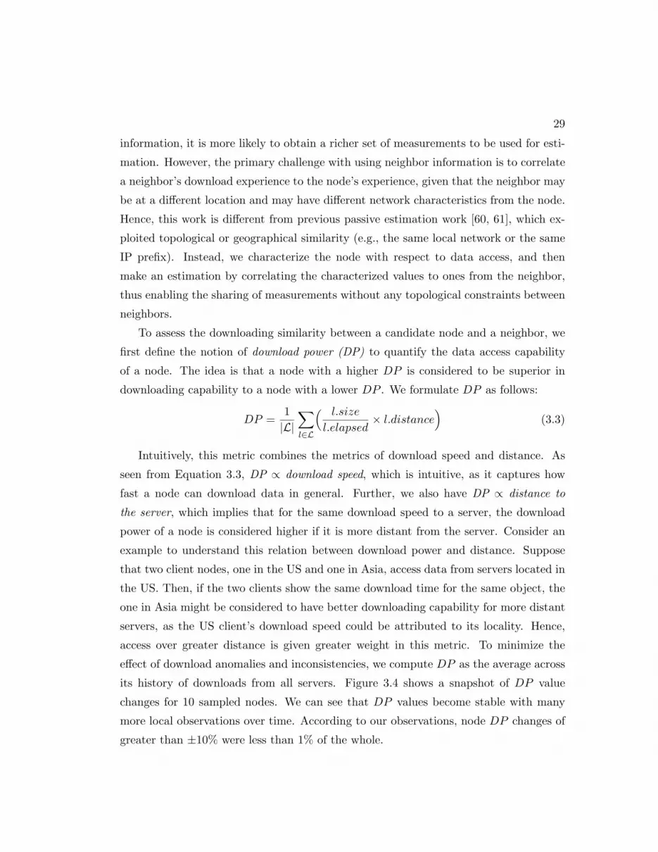
its history of downloads from all servers. Figure 3.4 shows a snapshot of DP value
changes for 10 sampled nodes. We can see that DP values become stable with many
more local observations over time. According to our observations, node DP changes of
greater than ±10% were less than 1% of the whole.

30
0 20 40 60 80 100500
1000
1500
2000
2500
3000
Time (number of computations of DP)
Com
pute
d D
P
DP changes over time
Figure 3.4: DP stability
With the characterized metric DP , we compute similarity between a candidate node
(i) and a neighbor node (j) by the following equation:
S(i, j, s) = DP (i)
DP (j)· distance(j, s)distance(i, s)
(3.4)
The scaling factor S is used to compare the download characteristics of any two un-
related nodes in the system to enable the appropriate scaling of neighbor measurements
for estimation. S(i, j, s) = 1 means that two nodes i and j are exactly the same with
respect to data retrieval from server s. If the scale value = 2, it means that the node
has a factor of two capability in accessing given server. Hence, S(i, j, s) < 1 indicates
that node i is inferior to node j in accessing server s, and vice-versa.
Now, we define a function for neighbor estimation at host i by using information
from neighbor j for object o:
NeighborEstim(o) = S(i, j, server(o))−1 × elapsed(o) (3.5)
Accessibility is expected download time; thus, it is inversely proportional to the

31
scaling factor, as shown in the equation. Note that server(o) and elapsed(o) are infor-
mation collected from a neighbor node, which stand for the server for object o and the
downloading elapsed time for o the neighbor observed, respectively. It is possible that
the neighbor has multiple measurements for the same object, in which case, we pick the
smallest download time (for elapsed(o) in the equation) as the representative.
Intuitively, to estimate the download time for object o based on the information from
neighbor n, this function uses the relevant download time of the neighbor. As a rule, the
estimation result is the same if all conditions are equivalent to the neighbor. To account
for differences, we employ a scaling factor. The first part of the scaling factor compares
the download powers of the node and the neighbor for similarity. If the DP of the node
is higher than that of the neighbor, the function gives a smaller estimation time because
the node is considered superior to the neighbor in terms of accessibility. The second
part of the scaling factor compares the distances to the server, so that if the distance
to the server is closer for the node than it is for the neighbor, the resulting estimation
will be smaller.4 These correlations enable us to share observations between neighbors
without any topological restrictions.
Figure 3.5 illustrates the cumulative distribution of relative errors of neighbor esti-
mation results, performed with the same data set used in self-estimation. As seen from
the figure, a substantial portion of the estimated values are located within a factor of 2.
Similar with the self-estimation results, nearly 90% of estimations reside within a fac-
tor of two, compared to the corresponding measurements. This suggests that neighbor
estimation produces useful information to rank nodes with respect to accessibility.
While neighbor estimation is useful for the assessment of accessibility, multiple neigh-
bors can provide different information for the same object. For example, if three neigh-
bors offer their observations to a node, there can be three estimates that may have
different values. Thus, we can combine those different estimates to obtain more accu-
rate results. We examined several combination functions, such as median, truncated
mean, and weighted mean, and observed that taking the median value works well, even
with a small number of neighbors. Given that the number of neighbors providing rel-
evant measurements may be limited in many cases, we believe that taking the median
should be a good choice.
4 We discuss how the server distance can be estimated without active probing in Section 3.2.5.

32
0 0.2 0.4 0.6 0.8 1 1.2 1.4 1.6 1.8 20
0.1
0.2
0.3
0.4
0.5
0.6
0.7
0.8
0.9
1
Relative Error
Cum
ulat
ive
Fra
ctio
n
Neighbor Estimation Result
Figure 3.5: Neighbor estimation relative error distribution
We observed that combining multiple estimates with the median function signifi-
cantly improves the accuracy. According to our simulation results, estimation with 4
neighbor measurements yielded nearly 90% of estimates within relative error 0.5, while
it was 84% with a single neighbor measurement. It becomes over 92% with 8 neighbor
measurements.
To realize neighbor estimation, it is necessary to gather information from the neigh-
bor nodes. This can be done by background communications; for example, piggybacking
on periodic heartbeats in the overlay network can be a practical option to save overhead.
3.2.5 Inferring Server Latency without Active Probing
While neighbor estimation requires latency to server as a parameter (Equation 3.5),
we can avoid the need for active probing by exploiting the server latency estimates
obtained from the neighbors themselves. If a neighbor has contacted the server, it could
obtain the latency at that time by using a simple latency computation technique, e.g.,
the time difference between TCP SYN and SYNACK when performing the download,
and this latency information can be offered to the neighbor nodes. By utilizing the
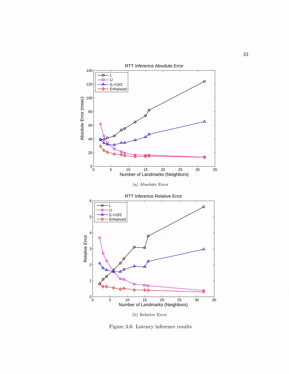
33
0 5 10 15 20 25 30 350
20
40
60
80
100
120
140
Number of Landmarks (Neighbors)
Abs
olut
e E
rror
(m
sec)
RTT Inference Absolute Error
LU(L+U)/2Enhanced
(a) Absolute Error
0 5 10 15 20 25 30 350
1
2
3
4
5
6
Number of Landmarks (Neighbors)
Rel
ativ
e E
rror
RTT Inference Relative Error
LU(L+U)/2Enhanced
(b) Relative Error
Figure 3.6: Latency inference results

34
latency information observed in the neighbor nodes, it is possible to minimize additional
overhead in estimation with respect to server location and pinging.
According to the study in [97], a significant portion of total paths (> 90%) satisfied
the property of triangle inequality. We also observed that 95% of total paths in our data
satisfied this property. The triangulated heuristic estimates the network distance based
on this property. It infers latency between peers with a set of landmarks, which hold
precalculated latency information between the peers and themselves [72]. The basic
idea is that the latency of node a and c may lie between |latency(a, b) − latency(b, c)|and latency(a, b) + latency(b, c), where b is one of the landmarks (b ∈ B). With a set
of landmarks, it is possible to obtain a set of lower bounds (LA) and upper bounds
(UA). If we define L = max(LA) and U = min(UA), then the range [L,U ] should be
the tightest stretch with which all inferred results may agree. For the inferred value,
Hotz [98] suggested L because it is admissible to use the A* search heuristic, while H
and all linear combinations of L are not admissible. Guyton and Schwartz [99] employed
(L+U)/2, and most recently Eugene and Zhang reported that U performs better than
the others [72].
In our system model, we can use neighbors as the landmarks because they hold
latency information, both to the candidate and to the object server. By applying the
triangulated heuristic, therefore, we can infer the latency between the candidate and the
server without probing. However, we found that the existing heuristics are inaccurate
with a small number of neighbors, which may be common in our system model. Hence,
we enhance the triangulated heuristic to account for a limited number of neighbors.
Our approach works by handling several situations that contribute to inaccuracy.
For example, it is possible to have L > U due to some outliers, for which the triangle
inequality does not hold. Consider the following situation: all but one landmark give
reasonable latencies, but if that one gives fairly large low and high bounds, the expected
convergence would not occur, thus leading to an inaccurate answer. To overcome this
problem, we remove all Li ∈ LA that are greater than U , so we can make a new range
that satisfies L < U . After doing so, we observed that taking the simple mean produces
much better results than the existing approaches.
We also observed a problematic situation where a significant portion of the inferred
low bounds suggest similar values, but high bounds have a certain degree of variance.

35
This happens where node c is close to a, but the landmarks are all apart from node a.
For this, we consider a weighted mean based on standard deviations (σ). The intuition
behind this is that if multiple inferred bounds suggest similar values for either low or
high bounds, it is likely that the real latency is around that point. We take the weighted
mean when it fails to converge, due to the range being too wide, where picking any one
of L, U , and (L+ U)/2 is likely to be highly inaccurate. The weighted mean is defined
as follows:
L ·(1− σLA
(σLA+ σUA
)
)+ U ·
(1− σUA
(σLA+ σUA
)
)We report the evaluation results with the absolute error, as well as the relative error
for clarity. For example, if we think of two measured latencies 1 ms and 100 ms, and
the corresponding estimations 2 ms and 200 ms, then those two estimations give the
same picture with respect to the relative error (i.e., relative error = 1, in this example).
In contrast, they convey different information with respect to absolute error. In fact, 1
ms difference is usually acceptable, but 100 ms error is not for latency inference.
Figure 3.6 demonstrates the inference results. As reported in [72], the heuristic
employing U is overall better than the other two existing heuristics. However, we can
see that our enhanced heuristic substantially outperforms the existing heuristics with
respect to both relative and absolute error metrics. In particular, the enhanced heuristic
works well, even when the number of landmarks is small. Since the number of neighbors
that can offer the relevant latency information may be limited, the enhanced heuristic
is desirable in our design. In other words, it is possible to infer the latency to the server
with fairly high accuracy, even in the case where only a few neighbor nodes can provide
relevant information.
3.3 Performance Evaluation
3.3.1 Experimental Setup
We conducted over 100K actual downloading experiments for a span of 5 months with
241 PlanetLab nodes geographically distributed across the globe. For this data collec-
tion, we first placed data files on randomly selected nodes, and then generated random

36
Table 3.1: Trace data (1MB–8MB)
Data Number of Number of Number of Mean Meansize traces nodes objects elapsed (sec) RTT (msec)
1M 22567 153 72 13.7 1032M 25957 230 82 22.4 1174M 28018 166 106 39.9 1028M 26237 159 85 67.4 101
queries for actual downloading. Before beginning the queries, all-pair pings were per-
formed 30 times for each pair of nodes, and the smallest RTTs were recorded as the
latency of the node pair. Finally, a thousand random queries were generated, and the
downloading elapsed times were recorded. For each query, we recorded the data object,
the client, the server, the latency, and the elapsed time for downloading. This data
collection was repeated multiple times to collect more records. Table 3.1 provides the
details of the download traces. In the simulations, we use a mixture of all traces rather
than individual traces, unless otherwise mentioned.
To evaluate resource selection techniques, we designed and implemented a simulator,
which inputs the ping maps and the collective downloading traces and outputs perfor-
mance results, according to the selection algorithms. Initially, the simulator constructs
a network in which nodes are randomly connected to each other with a predefined neigh-
bor size without any locality or topological considerations. To minimize error due to
the construction, we repeated simulations and reported the results with 95% confidence
intervals. After constructing the network, the simulator runs each resource selection
algorithm. Initially, it constructs a virtual trace in which the list of candidates and the
download time from each candidate are recorded. The candidate nodes are randomly
chosen for each allocation. As the candidate may have more than one actual download
record for a server, the download time is also randomly selected from them. The sim-
ulator then selects a worker based on each selection algorithm. Based on the selected
worker, the download time is returned from the virtual trace.
For our evaluation, we compared the resource selection techniques based on our
estimation techniques with two conventional techniques: random and latency-based

37
selections. The following describes the resource selection techniques, which choose one
computational resource from a given set of candidate nodes:
• Omni: Oracle-based selection
• Random: Random selection
• Proxim: Latency-based selection
• Self: Self performs the selection by self-estimation. One exception is that
it allows the node to make an estimation by direct measurements to the object
server, if any.5 This can improve accuracy. If no estimate is available, it
performs random selection.
• Neighbor: Neighbor performs the selection based on neighbor estimation. If
no estimate is available, it performs random selection.
To compare the different selection algorithms, we mainly used the metric Optimality
Ratio (O.R.), the ratio between the downloading elapsed time by the selection algorithm
and the downloading elapsed time by oracle selection. Thus, O.R. is equal to or greater
than 1 (O.R. ≥ 1), and O.R.=1 means the selection technique chooses optimal. Since
we used mixed data sets in simulation as mentioned, relative comparison is also more
meaningful than providing absolute download times.
3.3.2 Performance Comparison over Time
We begin by presenting the performance comparison over time. Figure 3.7 compares
the performance over 100K consecutive job allocations. As the default, we set both the
candidate size and the neighbor size to 8 (i.e., c = 8 and g = 8), but we will explore
a variety set of candidate and neighbor sizes, as well. Overall the proposed techniques
yield good results: Self is the best across time, and Neighbor works better than
Proxim most of the time. Random yields poor performance with a significant degree
of variation, as expected. Proxim is nearly 3 times of optimal, with a relatively high
degree of variation compared to the suggested techniques. Self works best approaching
5 This is done by a simple statistical estimator: size(o)
Throughput(s), where s is the server for object o,
and Throughput(s) stands for the mean download speed from server s.

38
0 1 2 3 4 5 6 7 8 9 10
x 104
1
2
3
4
5
6
7
8
9
10
Run
Opt
imal
ity R
atio
Performance comparison (c=8,g=8)
RANDOMPROXIMSELFNEIGHBOR
Figure 3.7: Performance over time
nearly 1.4 of optimal at the end of the simulation. This shows that simple consideration
of past access behavior in addition to latency greatly benefits choosing a good candidate.
Neighbor is poor at first, but outperforms Proxim after roughly 6K simulation
time steps. This is because there may be many more chances of random selection
initially; after warming up, however, it exploits neighbor measurements, leading to
better performance. Nonetheless,Neighbor still shows a noticeable gap to Self. This
can be explained mainly by the hit rate on the number of relevant measurements from the
neighbors; we observed that the average number of measurements was approximately
2, even at the end of the simulation, while neighbor estimation yields better results
with more than 4 measurements, as discussed in Section 3.2.4. Thus, Neighbor could
perform better with a higher hit rate. In the next chapter, we present the OPEN
framework, which is based on neighbor estimation, but utilizes proactive dissemination
of observed measurements for a greater hit rate and higher accuracy with many more
relevant measures.

39
3.3.3 Impact of Candidate Size
In our system model, a set of candidate nodes are evaluated for their accessibility before
allocating a job. We now investigate the impact of candidate size (c). Figure 3.8
demonstrates the performance changes with respect to candidate size. In Figure 3.8(a),
O.R. increases along the candidate size. This is becauseOmni has many more chances to
see better candidates to choose from, resulting in larger performance gaps. Nonetheless,
we can see that the suggested techniques work better with many more candidates,
making the slopes gentle compared to the conventional ones. Figure 3.8(b) compares
mean download time for the selection techniques. As seen in the figure, Self continues
to produce diminished elapsed times as the candidate size increases, yielding the best
results among selection techniques. Neighbor follows Self, with considerable gaps
against the conventional techniques. Interestingly, Proxim shows unstable results, with
greater fluctuation than Random over the candidate sizes. This result indicates that
the proposed techniques not only work better than conventional ones across candidate
sizes, but also further improve as the candidate size increases.
3.3.4 Impact of Neighbor Size
We next investigate the impact of neighbor size on Neighbor (the other heuristics
are not affected by this parameter). Figure 3.9 shows how the selection techniques
respond across the number of neighbors (g). As can be seen in the figures, increasing
the neighbor size dramatically improves the performance, while the others make no
changes, as expected. For example, the average download time in g = 16 is dropped to
approximately 70% of the time for g = 2. The O.R. is also dropped from 4.0 at g = 2
to 2.6 at g = 16. This is because it has more chances to obtain relevant measurements
with many more neighbors, thus decreasing the possibility of random selection. This
result suggests thatNeighbor will work better in environments where the node collects
measurement information from a greater number of neighbor nodes. This is the primary
motivation of the OPEN framework discussed in the next chapter.

40
2 4 8 16 321
2
3
4
5
6
7
8
9
Candidate Size
Opt
imal
ity R
atio
Impact of Candidate Size (g=8, Run=50k)
RANDOMPROXIMSELFNEIGHBOR
(a) Optimality ratio
2 4 8 16 320
10
20
30
40
50
60
70
80
90
Candidate Size
Dow
nloa
d T
ime
(sec
)
Impact of Candidate Size (g=8, Run=50k)
OMNIRANDOMPROXIMSELFNEIGHBOR
(b) Download elapsed time
Figure 3.8: Impact of candidate size

41
2 4 8 16 321
2
3
4
5
6
7
Neighbor Size
Opt
imal
ity R
atio
Impact of Neighbor Size (c=8, Run=50k)
RANDOMPROXIMSELFNEIGHBOR
Figure 3.9: Impact of neighbor size
3.3.5 Impact of Data Size
We next investigate how the selection techniques work over different data sizes. Since
the size of accessed objects can vary, depending on applications in reality, selection
techniques should work consistently across a range of data sizes. In this experiment,
we ran the simulation with individual traces rather than the mixture of the traces. In
Figure 3.10, we can see a linear relationship between data size and mean download
time. However, each technique shows a different degree of slope: Self and Neighbor
increase more gently than the conventional heuristics. With simple calculation, the
slopes (i.e., ∆y/∆x) of the techniques are Random=10.9, Proxim=8.1, Self=3.8,
and Neighbor=5.1. This result implies that the proposed techniques not only work
consistently across different data sizes, but they are also much more useful for data-
intensive applications.

42
1MB 2MB 4MB 8MB0
10
20
30
40
50
60
70
80
90
100
Data Size
Dow
nloa
d T
ime
(sec
)
Impact of Data Size (c=8, g=8, Run=50k)
OMNIRANDOMPROXIMSELFNEIGHBOR
Figure 3.10: Impact of data size
3.3.6 Timeliness
While it is crucial to choose good nodes for job allocation, it is also important to avoid bad
nodes when making a decision. For instance, selecting intolerably slow connections may
lead to job incompletion, due to excessive downloading cost or time-outs. However, it is
almost impossible to pick good nodes every time because there are many contributing
factors.
We observed how many times the techniques choose slow connections. Figure 3.11
shows the cumulative distributions of the speed of connections with log-log scales, and
we can see that the proposed techniques more often avoid slow connections. Self most
successfully excludes low speed connections, and Neighbor also performs better than
the conventional techniques. When we count the number of poor connections selected,
Self chose connections under 5KB/s fewer than 30 times, while Proxim made over
290 selections, which is almost an order of magnitude larger than Self. One interesting
result is that Proxim selects poor connections more frequently than Random (293
and 194 times respectively). This implies that relying only on latency information

43
10−1
100
101
102
103
104
10−5
10−4
10−3
10−2
10−1
100
Download Speed (KB/s)
Cum
ulat
ive
Fra
ctio
n
CDFs of Download Speed (c=8, g=8, Run=100k)
SELF
NEIGHBOR
RANDOM
PROXIM
Figure 3.11: Cumulative distribution of download speed
alone greatly increases the chance of very poor connections, thus leading to unpredictable
response time. This indicates that latency is useful, but not a perfect predictor of data
access performance. Compared to this, our proposed techniques successfully reduce
chances to choose low speed connections by taking data accessibility into account.
3.3.7 Multi-object Access
Many distributed applications request multiple objects [100], which means that the
associated jobs of such applications access more than one object to complete the task.
For example, the SkyServer database [101] in astronomy, scaling up to terabytes of
data, is constructed over multiple distributed servers, and a query can retrieve a set of
data objects (rather than a single object) to create appropriate results. We conducted
experiments to see the impact of multi-object access. Figure 3.12 shows the results
where jobs are required to access multiple objects. As can be seen in the figure, the O.R.
gradually decreases with an increasing number of objects for all selection techniques.
This is because even optimally selected nodes may not have good performance to some

44
1 2 4 81
1.5
2
2.5
3
3.5
4
4.5
5
5.5
Number of objects to access
Opt
imal
ity R
atio
Multi−object access (c=8, g=8, Run=50k)
RANDOMPROXIMSELFNEIGHBOR
Figure 3.12: Multi-object access
objects, resulting in greatly increased download times. Self and Neighbor not only
consistently outperform the conventional techniques over the number of objects, but
they also approach optimal (O.R. = 1.24 and 1.55) when the number of objects is 8.
To sum up, the suggested techniques also work better than the conventional techniques
for multi-object access.
3.3.8 Impact of Churn
Churn is prevalent in loosely-coupled distributed systems. To see the impact of churn, we
assume that mean session lengths of nodes are exponentially distributed. In this context,
the session length is equivalent to the simulation time. For example, if the session length
of a node is 100, the node changes its status to inactive after 100 simulation time steps.
The node then joins again after another 100 time steps. We assume that nodes lose all
past observations when they change status. Therefore, churn will have a greater impact
on our selection techniques because we rely on historic observations. In contrast, the
conventional techniques suffer little from churn since they do not have any dependence

45
on past observations. The virtual trace excludes objects for which the relevant servers
are inactive. We tested three mean session lengths: s = 100, s = 1000, and s = 10000,
corresponding to extreme, severe, and light churn rates, respectively.
Figure 3.13 illustrates the impact of churn. As mentioned, there is little impact
on conventional techniques, while our techniques are degraded in performance, due to
loss of observations. In Figure 3.13(a), Self is comparable to Proxim, even under
extreme churn. Neighbor degrades and becomes worse than Proxim under severe
churn (s = 1000). This is because Neighbor is likely to fail to collect the rele-
vant measurements, thus relying more on random selection, while Self can perform
fairly accurate estimation with only a dozen of measurements. Nonetheless, Neigh-
bor still works better than Proxim in light churn (s = 10000) with lower overhead.
Figure 3.13(b) explains why Neighbor suffers under severe and extreme churn. In
the figure, the neighbor estimation rate represents the fraction that Neighbor suc-
cessfully estimates, based on neighbor estimation rather than random selection. Under
light churn, the neighbor estimation rate is still over 90%, but drops to 60–70% in se-
vere churn, implying that 30–40% of the decisions have been made by random selection.
Under extreme churn, the neighbor estimation rate drops below 10%, so it essentially
reduces to Random.
To summarize, the proposed techniques are fairly stable under churn in which nodes
suffer from loss of observations. The results show that Self is comparable to Proxim,
even under extreme churn, while Neighbor is comparable to Proxim when churn is
light.
3.3.9 Impact of Replication
In loosely-coupled distributed systems, replication is often used to disseminate objects
to provide locality in data access, as well as high availability. We investigate the im-
pact of replication to see if the proposed techniques consistently work in replicated
environments.
For this, we construct replicated environments in which same-sized objects in the
traces are grouped according to the replication factor, and the object in the group is
considered as a replica. The virtual trace is then constructed, based on the group of
the objects. In detail, for all objects in the group, a randomly selected download time

46
No churn 10000 1000 1000
10
20
30
40
50
60
70
Mean Session Length
Dow
nloa
d T
ime
(sec
)
Impact of Churn (c=8, g=8, Run=50k)
OMNIRANDOMPROXIMSELFNEIGHBOR
(a) Download elapsed time
0 1 2 3 4 5 6 7 8 9 10
x 104
0
10
20
30
40
50
60
70
80
90
100
Run
Nei
ghbo
r E
stim
atio
n R
ate
(%)
Neighbor Estimation Rate (c=8, g=8, Run=100k)
No churnSessionLength=100SessionLength=1000SessionLength=10000
(b) Neighbor estimation rate
Figure 3.13: Impact of churn

47
from each candidate is recorded in the virtual trace. The simulator then returns the
download time, according to the selected candidate and the replica server.
Random will work the same as in the single replica environment with a random
function to choose both a candidate and a replica server. Proxim measures latencies
from every candidate to every server, and then the pair with the smallest latency will
be selected. Self is similar to Proxim: each candidate calculates the accessibility for
each server and reports the best one. In the case of Neighbor, the candidate gathers
all of the relevant information from the neighbors. If it finds more than one server,
NeighborEstim(o) function is performed against each server, and then the best one is
reported to the initiator. For both Self and Neighbor, the initiator finally selects
the candidate with the best accessibility.
Figure 3.14 shows performance changes across replication factors (r). It is likely
that the performance of all selection techniques improve as the replication factor in-
creases because of data locality, and the result agrees with this expectation, as shown
in Figure 3.14(b). Proxim has significantly diminished mean download time (nearly
half) under replication, but it is still worse than the proposed techniques. Self and
Neighbor outperform the conventional techniques over all of the replication factors.
In Figure 3.14(a), we can see that Self further reduces O.R. as the replication factor
increases, while the others increase. Neighbor widens the gap against conventional
techniques with an increasing replication factor.
Next, we investigate the impact of churn in replicated environments. First, we fix
the replication factor at 4 and observe the performance change over a set of mean
session lengths. As can be seen in Figure 3.15(a), the results are fairly similar with the
ones under churn in the non-replicated environment. However, Self is a little worse
than Proxim under extreme churn. Neighbor is comparable to Proxim under
light churn, but degrades under severe and extreme churn as in no replication. Then
we investigate performance sensitivity to the replication factor under light churn (i.e.,
s = 10000). As seen in Figure 3.15(b), Self is much better than Proxim across
all replication factors. Neighbor is fairly comparable to Proxim under light churn,
despite a greater chance of random selection.
To summarize, the proposed selection techniques consistently outperform the con-
ventional techniques in replicated environments. The results under churn are fairly

48
consistent with the results without replication: Self is comparable to Proxim under
severe churn, and Neighbor is comparable to Proxim under light churn.
3.4 Summary
While data availability indicates whether any instance of an object is available in the
system, data accessibility defines how efficiently a node can access a given data object
in the system. Thus, data accessibility is a crucial concern for an increasing number of
data-intensive applications in large-scale distributed systems.
In this work, we proposed novel techniques to estimate accessibility based on lo-
cal, historic information. Self-estimation makes accessibility estimation based on past
measurements in the local node, while neighbor estimation utilizes past measurements
collected in neighbor nodes in the overlay network. The simulation results indicate that
the proposed estimation techniques are sufficiently accurate in providing a meaningful
rank order of nodes, based on their accessibility. The proposed techniques outperform
conventional approaches for resource selection. In particular, selection based on self-
estimation approached 1.4 of optimal over time, and the neighbor estimation-based
selection was within 2.6 of optimal with 16 neighbors, compared to a latency-based
selection that was over 3 times the optimal. With respect to the mean elapsed time,
the self and neighbor estimation-based selections were 52% and 70% more efficient than
latency-based selection, respectively. We also investigated how the proposed techniques
work under node churn and showed that they work well under churn circumstances in
which nodes suffer from loss of observations. The overall simulation results show that the
proposed techniques consistently outperform conventional techniques in diverse working
conditions, including replicated environments.

49
1 2 4 81
2
3
4
5
6
7
8
9
10
11
12
Replication Factor
Opt
imal
ity R
atio
Impact of Replication (c=8, g=8, Run=50k)
RANDOMPROXIMSELFNEIGHBOR
(a) Optimality ratio
1 2 4 80
10
20
30
40
50
60
Replication Factor
Dow
nloa
d T
ime
(sec
)
Impact of Replication (c=8, g=8, Run=50k)
OMNIRANDOMPROXIMSELFNEIGHBOR
(b) Download elapsed time
Figure 3.14: Performance under replicated environments

50
No churn S=10000 S=1000 S=1000
1
2
3
4
5
6
7
8
9
10
11
Mean Session Length
Opt
imal
ity R
atio
Churn under Replication (c=8, g=8, r=4, Run=50k)
RANDOMPROXIMSELFNEIGHBOR
(a) Replication factor = 4
1 2 4 81
2
3
4
5
6
7
8
9
10
Replication Factor
Opt
imal
ity R
atio
Churn under Replication (c=8, g=8, s=10000, Run=50k)
RANDOMPROXIMSELFNEIGHBOR
(b) Mean session length = 10000 (light churn)
Figure 3.15: Impact of churn under replication
Chapter 4
OPEN: A Framework for
Accessibility Estimation
In the previous chapter, we presented estimation techniques for data accessibility based
on historical measurement information. In this chapter, we present a framework for scal-
able accessibility estimation based on neighbor estimation. The reason we use neighbor
estimation (rather than self-estimation) is that self-estimation cannot work better than
latency-based techniques for replica selection, as the only discriminator in self-estimation
is latency for replica selection. In contrast, neighbor estimation can distinguish better
servers by utilizing past measurement information if any neighbor node downloaded
from the servers. In addition, we observed that the accuracy of neighbor estimation
can be improved with a greater number of neighbor measurements. The framework
we present in this chapter proactively disseminates measurements to improve both the
hit rate and accuracy of estimation. In this chapter, we discuss how we can achieve
cost-effective dissemination for measurement sharing across the system, but without
significant performance loss.
4.1 Introduction
A key requirement for achieving data access predictability is the ability to estimate
network performance for data transfer, so that computation tasks can take advantage
of the estimation in their deployment or data source selection. In other words, network
51

52
performance estimation can provide a helpful guide to run data-intensive tasks in such
unpredictable infrastructures having a high degree of variability in terms of data access.
Active probing can be an option for estimation, but is unscalable and expensive in us-
ing back-to-back measurement packets. Passive estimation is attractive for its relatively
small overhead, and thus could be desirable for many networked applications that do
not require an extremely high degree of accuracy such as that needed by network-level
applications like network planning. For example, a substantial number of networked
applications, such as Web server selection and peer selection for file sharing, rely on
ranking. According to a peer-to-peer measurement study in [58], the second placed peer
performance is only 73% of the best peer performance. This significant gap implies that
some degree of estimation inaccuracy would be tolerable for such ranking-based appli-
cations. A potential problem of passive estimation is that it can suffer from estimation
failure due to the unavailability of past measurements. This problem can be mitigated
by sharing measurements among nodes; thus, a node can estimate performance even
against a server it has never contacted. In previous work [60, 61], however, the shar-
ing was restricted to specific underlying topologies such as a local network, limiting
scalability. In this work, we present a novel approach enabling nodes to utilize past
measurement information with no reliance on topological similarities, so as to minimize
blind spots in the system and to reduce uncertainty in data access.
In the previous chapter, we discussed how we can estimate data accessibility based
on past measurements without relying on explicit probing. In particular, neighbor esti-
mation enables nodes to utilize past measurements experienced by their neighbor nodes
without requiring any similarities on topology and system specifications. While neigh-
bor estimation was used in a more restricted environment (a small set of neighboring
nodes), and thus limited with respect to scalability and accuracy in the previous chapter,
we show how it can be extended by system-wide sharing of past measurements in this
chapter. One important challenge is how to facilitate local measurements to be globally
available to other nodes in the system for system-wide sharing. Any server-based tech-
niques for storing global information are limited by well-known problems of scalability
and fault tolerance. At the other end of the spectrum is flooding-based dissemination,
which while fully distributed, has high network overhead. In this work, we present
OPEN (Overlay Passive Estimation of Network Performance), a scalable framework

53
Table 4.1: Degree of measurement sharingDegree Pair-level Domain-level System-wide
Approach Statistical estimation Sharing in a LAN Sharing in a systemTime-series forecast Sharing in a domain
System/ NWS [68] SPAND [60] OPENTechnique HB prediction [77] Webmapper [61]
for accessibility estimation, based on passive estimation and proactive measurement
dissemination. OPEN is scalable, lightweight, decentralized, and topology-neutral.
The rest of this chapter is organized as follows. In the next section, we discuss the
degree of measurement sharing in estimation, and show why secondhand measurement-
based estimation is attractive in large-scale settings. Section 4.3 introduces the OPEN
framework with the core functionality of passive estimation and measurement dissemi-
nation. Then, we report our experimental results in Section 4.4 with respect to selection
performance and dissemination overheads. Finally, we provide a summary in Section 4.5.
4.2 Secondhand Estimation
We classify estimation techniques into the following three categories, based on the degree
of measurement sharing for their estimation: pair-level, domain-level, and system-wide,
as summarized in Table 4.1. Pair-level sharing only utilizes the direct (firsthand) mea-
surements made by a specific pair of nodes for their network path estimation. Many
statistical or time-series forecasting techniques, such as exponential moving average,
belong to this class. Previous studies [68] showed the high accuracy of these techniques,
but this class requires O(n2) measurements for estimation between all pairs.
In contrast, some estimation techniques enables nodes to utilize indirect (second-
hand) measurements provided by other nodes for their own estimation. In domain-level
sharing, past measurements in a domain (e.g., a single network or logical group of
nodes) are shared between nodes belonging to the same domain. In SPAND [60], nodes
in a single network share past measurements for Web server selection. Webmapper [61]
shares passive measurements to select a Web server based on a logical group clustered
by IP prefixes. By sharing the measurements in a domain, it is possible to estimate

54
performance if any node in the domain has communicated with the server. Again, how-
ever, the sharing is restricted to the domain. In addition, the underlying assumption
of existing techniques belonging to this class is that the nodes in a domain have closely
similar characteristics in network access. If this is not the case, sharing measurements
without considering node characteristics may cause inaccuracy in estimation.
Unlike the above two classes of sharing, system-wide sharing, which we propose in
this work, has no constraints on sharing measurements across the system. In other
words, if any measurement against a server is available in the system, any other node
can utilize that information for its own estimation to that server. Thus it is possible
to perform any-pair estimation with O(n) measurements. Since it does not rely on
topological similarities, node characterization is essential to utilize others’ experiences.
In addition, efficient sharing is also a key for this approach. Before discussing how
OPEN realizes those key functions, we briefly describe the rationale for secondhand
estimation in large-scale infrastructures.
4.2.1 Why Secondhand Estimation?
Existing estimation techniques such as those providing pairwise estimates [68] rely on
firsthand (i.e., prior direct) measurements between node-server pairs to estimate future
performance for these pairs. While such estimates are likely to be more accurate than
using secondhand measurements (from other nodes), it is unlikely that all nodes will
have firsthand measurements to all servers (a worst-case of O(n2) total measurements
in the system if all workers are also data servers). Thus, there would be no estimates
available for node pairs that lack direct measurements.
Figure 4.1 compares the potential estimation failure rates of a pairwise firsthand esti-
mation technique to that of a system-wide secondhand estimation approach (OPEN) 1 ,
caused by a shortage of existing relevant measurements. This result is obtained through
a trace-driven simulation2 , where we tested 100,000 estimations in two systems with
size n = 100 and n = 1000. We assume there are no measurements at all in the begin-
ning, and one random pairwise measurement is recorded at each time instant. As can
1 OPEN uses dissemination of secondhand measurements, as will be discussed in more detail inSection 4.3.3.
2 We will present details of the trace and our methodology in Section 4.4.1.

55
0 20000 40000 60000 80000 1000000
10
20
30
40
50
60
70
80
90
100
Run
Fai
lure
rat
e in
est
imat
ion
(%)
Estimation failure rate
Pairwise (n=1000)
Pairwise (n=100)
OPEN (n=1000)
OPEN (n=100)
Figure 4.1: Hit rate of relevant measurements
be seen from the figure, the failure rates decrease as more measurements are added over
time. In particular, we observe that OPEN dramatically diminishes the failure rates
over time by using secondhand measurements for estimation. In contrast, the pairwise
firsthand technique suffers from significant failure rates; the system with n = 1000 has
over 90% failure, even at the end of the simulation. This is because the probability that
a node has any measurements to a server goes down as the system size grows. Given
that a large-scale system can consist of tens of thousands nodes, the pairwise approach
must ensure, in the worst case, that O(n2) measurements exist, which could require
active probes to fill in the gaps due to insufficient firsthand measurements; or it may
suffer from high failure rates due to a lack of sufficient measurements. Therefore, the
secondhand approach should be beneficial in terms of both scalability and overhead.
Again, domain-level sharing also performs secondhand estimation, but relies on
topological similarity. Our intention is to design a framework to enable secondhand
estimation without any topological constraints, as described in the next section.

56
(a) Data download (b) Dissemination of measure-ment
(c) Estimation with measure-ments
Figure 4.2: OPEN estimation and dissemination
4.3 The OPEN Framework
In this section, we introduce the OPEN framework, which provides passive estimation
for end-to-end network performance based on secondhand measurements from other
nodes.
To realize system-wide, topology-independent passive estimation, our framework
uses two mechanisms: estimation of network performance and dissemination of observed
measurements. Figure 4.2 briefly illustrates these mechanisms. After node A downloads
a data object from server S (4.2(a)), it passes the downloading information, including
its characterized metric, to neighbor nodes, and the information is disseminated across
the system (4.2(b)). Node C can then make a passive estimation to server S based on
the experience of A (4.2(c)). We now discuss how OPEN implements its functionality.
4.3.1 End-to-End Accessibility
In the previous chapter, we used the data accessibility metric to quantify application-
level communication cost in accessing a given data object. In this framework, we define
end-to-end accessibility to represent application-level network performance between a
client and a server for a scalability reason (under the assumption that the number of
nodes≪ the number of data objects). In other words, end-to-end accessibility represents
how accessible a server is to a specific client, while data accessibility represents how
accessible a data object is to a specific client. In this work, we use the expected download
speed (or throughput) as the metric to quantify end-to-end accessibility.

57
Table 4.2: Attributes of measurements
Attribute Description Which record
id Unique ID Both (L, I)client Measurement node Imported (I)server Data server Both (L, I)distance Distance to server Both (L, I)throughput Measured download speed (= size
elapsed) Both (L, I)DP Download power Imported (I)timestamp Time stamp Both (L, I)
4.3.2 Passive Estimation
OPEN utilizes two types of measurements for estimation for a node: local measurements
(L) measured directly by the node, and imported measurements (I) obtained from other
nodes. OPEN makes an estimation by comparing and combining the node capability in
data access from its local measurements to the imported measurements of other nodes,
as we will show. Table 4.2 summarizes the attributes defined in the local and imported
measurement records.
As in Chapter 3, we can compute the download power (DP) from the local measure-
ment table:
DP =1
|L|∑l∈L
(l.throughput× l.distance) (4.1)
The scaling factor S computes similarity of any two unrelated nodes to enable the
appropriate scaling of secondhand measurements for estimation:
S(i, j, s) = DP (i)
DP (j)· distance(j, s)distance(i, s)
(4.2)
In the scaling factor equation, all the terms except distance(i, s) can be obtained
from past measurements. Since distance is a function of latency, we can consider any
lightweight latency prediction technique for the term distance(i, s). For example, Vi-
valdi [70], which is also used in the SWORD resource discovery tool [46], can predict
latency based on piggybacking, thus minimizing explicit probing.
Based on the scaling factor, OPEN produces accessibility to a server by utilizing
an imported measurement with the same server. The following equation is used to

58
estimate end-to-end accessibility (Ae2e) between client h and server s with an imported
measurement m:
Ae2e(h, s) = S(h,m.client, s)×m.throughput (4.3)
If there exists multiple imported measurements to the same server, we take the
median estimate as the accessibility to the server, based on our observation as discussed
in Chapter 3.
Accuracy of estimation
To evaluate accuracy, we performed simulation with actual downloading traces summa-
rized in Table 4.3. In the simulation, 10,000 estimations were made by Equation 4.3,
and we computed relative error of estimates.
Figure 4.3 illustrates the cumulative distribution of the OPEN estimation results
with respect to relative error. The upside figure shows the impact of the number of
secondhand measurements, while the downside figure shows the impact of the number
of local measurements when the number of secondhand measurements is 4. As seen in
Figure 4.3(a), estimation with 4 secondhand measurements approximates to the best
result, yielding roughly 90% of estimations located within a factor of two. The esti-
mation with 2 secondhand measurements is still fine, but the accuracy drops quickly
when the number of secondhand measurements is only one. In Figure 4.3(b), we can
see that the estimation with a single local measurement poorly performs. However, it
performs quite well with 5 local measurements. It continuously improves with 10 local
measurements, but more than that does not further improve. These results indicate
that the OPEN framework enables nodes to participate in estimation without a costly
learning phase. In addition, it implies that storage requirements can be small.
We add comments on estimation accuracy. Of past estimation work, Spruce [95] is a
pairwise bandwidth estimation tool based on packet pairs. In their Internet experiments,
70% of the estimations are located within relative error 0.3, and roughly 80% and
90% are located within relative error 0.5 and 1 (i.e., a factor of two), respectively. In
GNP [72], a network coordinate system, the best result in estimating latency is that
approximately 90% and 95% are located within relative error 0.5 and 1, respectively.
Our results show that 60% of the estimates lie within relative error 0.3, and 77% and

59
0 0.5 1 1.5 2 2.5 3 3.5 40
0.2
0.4
0.6
0.8
1
Cum
ulat
ive
frac
tion
Performance by # relevant measures
# measures=1# measures=2# measures=4# measures=16
0 0.5 1 1.5 2 2.5 3 3.5 40
0.2
0.4
0.6
0.8
1
Relative error
Cum
ulat
ive
frac
tion
Performance by # local measures (# imported measures=4)
# local measures=1# local measures=5# local measures=10# local measures=100
(a) Impact of the number of relevant measures
(b) Impact of the number of local measures
Figure 4.3: Relative error of estimates
89% are in relative error 0.5 and 1, respectively. The OPEN estimation accuracy is
slightly below the Spruce’s, but recall that OPEN is not a pairwise estimation technique
utilizing firsthand measurements that Spruce does. Thus, it is not an unexpected result.
Nonetheless, we see that the number of estimates less than relative error 0.5 in OPEN
is almost comparable to the one in Spruce.
Since there is no topological dependence in this estimation process, any node can
utilize secondhand measurements that any other nodes experienced. Thus, the next
question is how we can efficiently share measurements across the system.

60
4.3.3 Proactive Dissemination
In the neighbor estimation technique discussed in Chapter 3, collecting secondhand
measurements for a node took place on demand by contacting its neighbor nodes in
the overlay network. This creates an additional delay for estimation. Moreover, this
technique may not be scalable, due to the increasing likelihood of miss rates when relying
only on neighbor experience. To address this limitation, OPEN performs proactive
dissemination by which nodes can utilize prior measurements experienced by other
nodes for their own estimations without delay. A challenge for this, however, is the
cost of measurement dissemination. In this section, we discuss how OPEN can achieve
proactive dissemination with limited overhead, but without significant performance loss.
Probabilistic dissemination
The simplest form of dissemination is to immediately forward new information to the
neighbors at every node. This would be helpful for quick propagation of the infor-
mation, but such flooding can critically disrupt user traffic, degrading overall system
performance.
The probabilistic approach can reduce such dissemination overhead by forwarding
the information to a partial set of neighbors (instead of all neighbors). In this technique,
dissemination probability (p) defines the probability that a node forwards disseminated
information to neighbor nodes. Thus p = 1 is equivalent to flooding, while p = 0 means
no dissemination at all. Once a node generates (or receives) new information, it forwards
the information based on p; thus, the average fanout is approximately p × g, where g
is the average number of neighbor nodes. While perfect in dissemination, flooding
makes a huge number of duplicate dissemination messages for the same information.
By assigning p < 1, thus, it is possible to reduce such duplications.
One more optimization to reduce dissemination overhead would be periodic dissemi-
nation. Unlike immediate forwarding, periodic dissemination holds new information for
a certain time period, thus enabling redundant information to be compressed. Then ac-
cumulated information is delivered at each time interval. Since many overlay networks
employ periodic heartbeats for a health check between neighbors, periodic dissemination
could be realized via piggybacking.

61
Probabilistic dissemination opens up a rich space of optimizations to the OPEN
framework. In addition to such probabilistic optimizations, OPEN provides further
optimizations, based on the “criticality” of the measurement; i.e., whether it is highly
important (or hot) to the system or relatively less important (or cold). We next intro-
duce two optimization techniques called selective eager dissemination, which dissemi-
nates hot information eagerly, but cold information periodically, and selective deferral
and release, which defers distribution unless the measurement is determined to be hot
within a time-bound.
Selective eager dissemination
Although periodic dissemination can greatly diminish the number of dissemination mes-
sages, one limitation with this technique is the propagation delay due to its periodicity.
Some applications need to spread critical information more quickly. For example, we
may want to disseminate the secondhand measurement if we have no information about
that server in the measurement yet, in order to reduce the potential miss rates in esti-
mation. To handle this, we consider selective eager dissemination, which disseminates
hot information quickly without delay, while cold information is delivered periodically.
In other words, only critical information is eagerly propagated to the system in this
technique.
Algorithm 1 illustrates the procedure of selective eager dissemination. Function
initiate is performed by a source node when a new measurement is obtained by actual
downloading, and the source node determines if the new measurement is worth being
distributed eagerly. Based on the decision, the measurement is either forwarded to
neighbors at once (if is eager(m) == true) or stored in the list for periodic dissemination
(if is eager(m) == false). A receiving node performs a similar function: it forwards the
information immediately if it is hot; otherwise, it is moved to the periodic forwarding
list, as seen in the receive function. Each node performs periodic dissemination when
the periodic timer expires by the timeout function. The internal functions can be
defined on the local state, as perceived by the initiating or receiving node.
Hot information can be determined in several ways such as by using repetitive coun-
ters, timestamps, statistical deviations, or any combination of these techniques. In this
work, we use a threshold, such that if the number of measurements for a server is below

62
Algorithm 1 Selective eager dissemination
1: initiate(message m):2: if is eager(m) == true then3: forward(m);4: else5: forwardList.append(m);6: end if
7: receive(message m):8: if message ∈ historyList then9: historyList.append(m);10: if is eager(m) == true then11: forward(m);12: else13: forwardList.append(m);14: end if15: end if
16: timeout():17: forward(forwardList);18: forwardList ← ∅
19: forward(message array m[]):20: N ← neighbor nodes;21: for all n ∈ N do22: if random() ≤ p then23: send m[] to n;24: end if25: end for
this threshold, then the server-specific measurement is more eagerly distributed. For
example, if a measurement is “below-threshold,” then a node would forward it without
any delay; otherwise, the measurement is regarded as cold. Thus, it is lazily forwarded
after the given periodic interval expires.
Selective deferral and release
Another optimization technique we introduce is selective dissemination based on deferral
and release conditions, which define whether new information can be deferred (for its
dissemination) or released (to the system). If a “deferral” decision is made for some new
information, the source node does not emit it into the system until the corresponding
“release” condition is met. Thus, the deferral condition tests if new information is
critical, while the release condition retests if deferred information is critical based on the
passage of time. In this technique, any deferred information will either be disseminated

63
if it becomes important later or discarded when it becomes stale. In contrast, selective
eager dissemination ultimately forwards all information.
The basic idea of this technique is to distribute a newly collected measurement
only if it offers unique information different from past measurements. For example,
suppose node A makes an estimation of 100KB/s for end-to-end throughput to node
B based on past shared measurements. Now assume node A just downloaded a data
object from B with 100KB/s throughput. Then node A may not want to disseminate
such redundant information to others (deferral). However, this cold information can
be changed to hot as more measurements are collected in the system. Continuing with
the above example, suppose node A later sees its estimation to B with newly collected
information to be significantly different from its own past measurement. For example,
for a new measurement of 10KB/s, node A may want to tell other nodes about the
deferred experience (release).
In this work, we establish a deferral condition and a release condition based on
the difference between new measurement and current estimation derived from prior
measurements. Suppose observed is a newly measured throughput to a specific server
and expected is the estimated throughput to that server, based on past measurements.
Deferral condition:|observed− expected|
observed< τ1
Thus, τ1 = 0 means no information will be deferred, whereas any arbitrary large
value of τ1 (e.g., τ1 = 100) may defer most of the newly collected measurements.
The release condition is similarly defined with the deferral condition by comparing
deferred measurement (deferred) and current estimation (expected), as follows:
Release condition:|deferred− expected|
deferred≥ τ2
Since expected is the estimated throughput with all past relevant measurements, it
can be different from the estimated value computed in the deferral phase. By this condi-
tion, if the deferred measurement has distinct information from the current estimation,
it begins to be disseminated.

64
Algorithm 2 Selective deferral and release
1: initiate(message m):2: if deferral cond(m) == true then3: deferredList.append(m);4: else5: forward(m);6: release test(m);7: end if
8: receive(message m):9: if message ∈ historyList then10: historyList.append(m);11: forward(m);12: release test(m);13: end if
14: release test(message m):15: D ← deferred messages to the same server as m from deferredList;16: for all d ∈ D do17: if release cond(m) == true then18: forward(d);19: deferredList.delete(d);20: end if21: end for
Defining τ -values can be system specific, depending on system-level requirements. In
Section 4.4.3, we examine how τ -values impact performance and dissemination overhead.
Algorithm 2 illustrates details of the selective deferral and release technique. As in
Algorithm 1, a node performs initiate when it obtains a new measurement, while non-
source nodes perform receive when they receive dissemination messages from neighbors.
If the measured information is hot to the system (i.e., deferral cond(m) == false), it is
immediately disseminated; otherwise, it is put in the deferred list, as seen in initiate.
As before, these functions can be defined on the local node state. Any receiving node
stores new information and simply forwards it if it has not seen the information before,
as shown in the receive function. In both initiate and receive, a release test follows
after new information is forwarded. This checks whether any prior deferred information
is now hot and can be distributed, as shown in release test. Although not shown
explicitly in the algorithm, deferred messages will be purged, based on their age.

65
Table 4.3: Trace data (including 16MB)
Data Number of Number of Number of Mean Meansize traces nodes objects elapsed (sec) RTT (msec)
1M 22567 153 72 13.7 1032M 25957 230 82 22.4 1174M 28018 166 106 39.9 1028M 26237 159 85 67.4 10116M 11795 128 102 164.2 98
4.4 Evaluation
We now present results from an evaluation of OPEN using a trace-based simulation.
We first describe our simulation methodology, followed by performance results for the
two selection problems; i.e., resource selection and replica selection. Then, we examine
the dissemination overhead of OPEN.
4.4.1 Evaluation Methodology
As described in Section 3.3.1, we collected download traces from PlanetLab. In addition
to the traces in Table 3.1, we further collected 16MB downloading traces based on an
analysis of GridFTP traces [35]. Table 4.3 provides the details of the download traces,
including new 16MB traces. The simulator is also extended to support measurement
dissemination functions.
We demonstrate evaluation results for three systems according to the scale, Small
(n = 242), Medium (n = 1210), and Large (n = 12100), but focus more on the large-
scale system. We scaled the simulated system by allocating multiple simulated nodes
to the same trace data node. Candidate size (c) is the number of candidate nodes for
resource selection, while replication factor (r) is the number of replicas holding a data
object.
For evaluation, we compare our OPEN-estimation based selection (Open) with a
diverse set of selection techniques. These include random selection (Random) that
randomly selects a node, and latency-based selection (Proxim) that finds a client-
server pair with the smallest RTT. In addition, we consider selection based on several

66
pairwise estimation techniques that use only firsthand measurements. These techniques
include statistical mean, median, exponential smoothing, and last value; we select the
best one of this group and call it Pairwise. For all estimation techniques, we assume
an infinite window size; thus, all past measurements are used in estimation.
Unlike Random and Proxim, the other selection techniques can suffer from esti-
mation failures due to a shortage of relevant measurements.3 To avoid meaningless
estimation values from impacting the selection algorithm, we use the Pairwise and
Open estimation techniques only if at least half of the measurements required for es-
timation are available, based on our observation that performance gets degraded if we
perform selection with less than half; otherwise, we assume that the selection using
these techniques falls back on latency-based selection.
To compare performance of selection algorithms, we mainly use the metric Opti-
mality Ratio (O.R.), introduced in Section 3.3.1. We also examine the overhead of
dissemination. For this, we evaluate the number of messages generated for dissemina-
tion of measurements to share in the system.
4.4.2 Selection Performance
We present our trace-based experimental results with respect to the two selection prob-
lems described earlier: replica selection to choose one of the replicated servers and
resource selection to choose a computational resource for task allocation. In this sec-
tion, we assume complete sharing of secondhand measurement information to show the
benefit of this information. In the following section, we will discuss the overheads of
sharing, and how these costs can be reduced.
Performance comparison
We begin by demonstrating the performance results in three different scaled systems.
Figure 4.4 shows the results for both replica selection (r = 8) and resource selection
(c = 8). In the small-sized system, Pairwise outperforms Proxim, agreeing with
the intuition that considering network throughput works better than relying on latency
3 Proxim does not fail since the trace data include latency information.

67
Small Medium Large1
2
3
4
5
6
7
8
System Size
Opt
imal
ity R
atio
Replica Selection (r=8,Run=50k)
RANDOMPROXIMPAIRWISEOPEN
(a) Replica selection
Small Medium Large1
2
3
4
5
6
7
8
System Size
Opt
imal
ity R
atio
Resource Selection (c=8,Run=50k)
RANDOMPROXIMPAIRWISEOPEN
(b) Resource selection
Figure 4.4: Performance comparison

68
information for bandwidth-demanding applications. Similarly, Open significantly out-
performs Proxim by utilizing past measurements accrued in the system. We can see
that Open and Pairwise are fairly comparable in the Small system.
However, Pairwise significantly degrades as the system scales up, yielding nearly
equivalent results to Proxim. This is because, as discussed in Section 4.2.1, there is a
high probability that the pairwise techniques fail to see relevant measurements in their
estimations, and hence will fall back to Proxim. In replica selection, the fallback ratio
to Proxim is 15% in the Small system, but increases by 95% in the Medium system.
In the Large system, it becomes almost 100%, indicating that no pairwise estimation
was made, due to a lack of pair-level measurements. In contrast, Open falls back
to Proxim 0.5% in the Small system, 2% in the Medium system, and 18% in the
Large system. This result emphasizes again why secondhand estimation is attractive for
large-scale systems.
The fallback ratios for Pairwise are greater in resource selection; it is 24% in
the Small system, while it is 15% for replica selection, which explains why Pairwise
shows better performance in replica selection in the Small system in Figure 4.4. Unlike
this, Open shows similar fallback ratios between the two selections. In the Large
system, Open requires more time to collect measurements for each server. This slightly
increases O.R. than the smaller systems in the Large system.
Although Open shows good performance compared to other techniques, the results
might depend on environmental factors. To examine this, we next perform experiments
with a different number of servers and data access patterns.
Impact of the number of servers
We next study the impact of the number of servers (s) on the performance of the different
techniques. Intuitively, having fewer servers is likely to help Pairwise, as there would
be a greater likelihood of pairwise measurements to these servers being available. In
this experiment, we set up three configurations: a small dedicated server environment
(s = 10), a peer-to-peer computing environment in which any node can work as a server
(s = All), and a medium in which roughly 10% of nodes work as data servers (s = 100).
Since we observed that Pairwise does not make any difference from Proxim in the
large-scale setting, we perform this experiment in the Medium system to closely see the

69
s=10 s=100 s=All s=10 s=100 s=All1
2
3
4
5
6
7
8
Replica Selection Resource Selection
Opt
imal
ity R
atio
Number of Servers (Medium,Run=50k)
RANDOMPROXIMPAIRWISEOPEN
Figure 4.5: Impact of the number of servers
impact of the number of servers.
Figure 4.5 shows performance results. With small, dedicated servers (i.e., s = 10 and
s = 100), we can see a high degree of variations in both replica and resource selections.
This is because the results should depend on the chosen servers more in a relatively
small number of server environments. Despite the variations, the results show that
Open outperforms all the other techniques in diverse environments with a different
number of servers.
Impact of data access patterns
We next investigate the impact of the data access pattern. Up to now, we have assumed
uniform data access. In reality, however, data access distribution can be skewed; thus,
some objects can be more frequently retrieved [40, 102, 103, 104], showing a Zipf-like
distribution in which access frequency of the ith-most popular object is proportional to
i−α, where α is the Zipf parameter determining skewness.
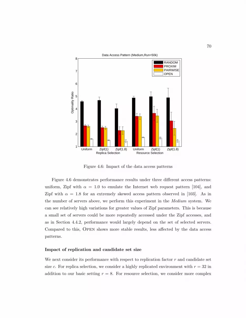
70
Uniform Zipf(1) Zipf(1.8) Uniform Zipf(1) Zipf(1.8)1
2
3
4
5
6
7
8
Replica Selection Resource Selection
Opt
imal
ity R
atio
Data Access Pattern (Medium,Run=50k)
RANDOMPROXIMPAIRWISEOPEN
Figure 4.6: Impact of the data access patterns
Figure 4.6 demonstrates performance results under three different access patterns:
uniform, Zipf with α = 1.0 to emulate the Internet web request pattern [104], and
Zipf with α = 1.8 for an extremely skewed access pattern observed in [103]. As in
the number of servers above, we perform this experiment in the Medium system. We
can see relatively high variations for greater values of Zipf parameters. This is because
a small set of servers could be more repeatedly accessed under the Zipf accesses, and
as in Section 4.4.2, performance would largely depend on the set of selected servers.
Compared to this, Open shows more stable results, less affected by the data access
patterns.
Impact of replication and candidate set size
We next consider its performance with respect to replication factor r and candidate set
size c. For replica selection, we consider a highly replicated environment with r = 32 in
addition to our basic setting r = 8. For resource selection, we consider more complex

71
c=1,r=8 c=1,r=32 c=8,r=1 c=32,r=1 c=8,r=81
2
3
4
5
6
7
8
9
Opt
imal
ity R
atio
Replica Selection (Large,Run=50k)
RANDOMPROXIMPAIRWISEOPEN
Figure 4.7: Impact of replication and candidate size
settings with candidate size and replication factor. We test following three settings:
c = 8 and r = 1 (i.e., no replication), c = 32 and r = 1 (i.e., a greater set of candidates),
and c = 8, r = 8 (i.e., resource selection in a replicated environment).
Figure 4.7 shows that Open is superior to the other techniques under the diverse
settings. In addition to O.R., Table 4.4 shows mean downloading time in milliseconds
and how much Open saves compared to Proxim. This includes the learning phase
where Open relies on latency information. When we compute mean elapsed time
after excluding this learning phase performance, we obtain 35% saving on average,
compared to 27% saving, including the learning phase performance. In the table, the
95% confidence intervals are smaller than 1.5 seconds.
We showed that Open consistently outperforms the other techniques in diverse
settings, as well as various working environments. We next examine the overhead of the
OPEN framework and discuss how to handle the dissemination overhead with minimal
performance loss.

72
Table 4.4: Mean downloading timeReplication Candidate Proxim Open Saving
factor size (sec) (sec)
8 1 44.1 33.5 24%32 1 39.3 30.9 21%1 8 62.6 43.8 30%1 32 45.8 34.4 25%8 8 27.4 17.5 36%
4.4.3 Overhead Optimization
Open needs to share measurements among nodes for secondhand estimation. In the
previous section, we simply assumed that all past measurements are available to all
nodes by the flooding of measurements. In this section, we show how we can optimize
the cost of measurement sharing.
Selective eager dissemination
We first examine the performance and overhead of selective eager dissemination. With
this technique, critical information is distributed without any delay, while non-critical
information relies on periodic, lazy dissemination. Recall that the decision as to whether
new measurement is critical is based on a counter determining how many measurements
have been propagated for that server. If the counter value is below the predetermined
threshold, the measurement will eagerly be distributed; otherwise, it should wait until
next periodic timer goes off.
For evaluation, we examine three different settings: Flooding, Periodic with an in-
terval of 1000, and Eager with the same interval, but with an eager threshold of 2. In
other words, with Eager, any new measurements will be eagerly forwarded if the node
has seen fewer than 2 measurements for the corresponding server, while others will be
periodically disseminated with the interval. Figure 4.8 presents experimental results in
replica selection with replication r = 8 in the Large system. We assumed that node
degree (the number of neighbor nodes) is uniformly distributed between 2 and 8. In
Figure 4.8(a), we can see that Periodic suffers from performance degradation due to the
large dissemination interval at the first stage of the time, showing almost similar results

73
0 10000 20000 30000 40000 500001.5
2
2.5
3
3.5
4
Run
Opt
imal
ity R
atio
Replica Selection (Large,r=8)
PROXIMFloodingPeriodicEager
(a) Performance
0 10000 20000 30000 40000 500000
1
2
3
4
5
6
7x 10
7
Run
Num
ber
of m
essa
ges
Replica Selection (Large,r=8)
FloodingPeriodicEager
(b) Overhead
Figure 4.8: Selective eager dissemination

74
1
1.2
1.4
1.6
1.8
2
2.2
2.4
2.6
2.8
3
Opt
imal
ity R
atio
Replica Selection (Large,r=8,Run=50k)
Flooding Eager(1.0)
Eager(0.1)
Eager(0.2)
Eager(0.3)
Eager(0.5)
(a) Performance
0
0.5
1
1.5
2
2.5
3
3.5x 10
9
Num
ber
of d
isse
min
atio
n m
essa
ges
Replica Selection (Large,r=8,Run=50k)
Flooding
Eager(0.1)Eager(0.2)
Eager(0.3)
Eager(0.5)Eager(1.0)
(b) Overhead
Figure 4.9: Selective eager dissemination with dissemination probability

75
with Proxim. In contrast, Eager yields comparable performance to Flooding, even
from the first stage. Figure 4.8(b) shows the number of messages to disseminate mea-
surements. At the first stage, Eager creates a large number of dissemination messages,
but it is significantly reduced over time, approaching Periodic.
In the above experiment, the total number of dissemination messages for Eager
was ∼ 15% of the Flooding result. This can be further optimized by taking advantage
of dissemination probability. Figure 4.9 shows experimental results for selective eager
dissemination with diverse dissemination probabilities. In this experiment, we gave the
same interval and threshold as the above, but each Eager has a different dissemination
probability; for example, Eager(0.1) stands for selective eager dissemination with a
probability of 0.1. As seen in Figure 4.9(a), a small dissemination probability fails
sharing measurements; however, proper optimization, for example Eager(0.3), yields
fairly comparable results to flooding and Eager(1.0). In this case, the overhead is
further reduced to ∼ 30% of the Eager(1.0) result, equivalent to only ∼ 5% of Flooding.
Selective deferral and release
We next evaluate the selective deferral and release technique. Table 4.5 presents exper-
imental results in replica selection with replication r = 8 in the Large system with the
same node degree distribution in the above selective eager dissemination experiments
(i.e., the number of neighbor nodes is 2–8 for each node). In this experiment, we use
τ = τ1 = τ2 to make deferral and release decisions. A smaller τ would make deferral
decision less likely, whereas a greater τ tends to aggressively defer the dissemination of
new measurements. As shown in the table, we can see that performance degrades with
a greater τ value, due to the increasing number of deferred measurements. The number
of released measurements increases until τ = 0.25, but decreases as τ becomes greater.
This is because with a smaller τ value than 0.25, a large portion of measurements are
propagated without having been deferred; thus, they have a smaller chance of being
releasing later. However, with a greater τ , the release condition becomes stricter with
a greater τ value, thus suppressing the release of the deferred measurements. The table
shows a trade-off between performance and overhead, suggesting that a sweet spot lies
somewhere between τ = 0.25 and τ = 0.5.
Figure 4.10 plots the number of deferred and released measurements over time for

76
Table 4.5: Impact of selective deferral and releaseτ O.R. # Deferred # Released Saving
0 2.09 0 0 0%0.1 2.09 9359 4876 9%0.25 2.10 21266 7204 28%0.5 2.14 32846 4903 56%1 2.25 38875 488 77%
100 2.32 44573 0 89%
τ = 0.25 and τ = 0.5. Interestingly, the rate of message growth for deferred measure-
ments are greater than for released measurements, implying that saving will be greater
over time. The number of messages for deferred measurements are much more sensitive
to τ then for release. As seen in Table 4.5, however, 34% of deferred measurements are
released for τ = 0.25, while only 15% were released for τ = 0.5 with a tighter release
condition.
4.4.4 Simulation with S3 Data Sets
To test the generality of the framework, we conducted another simulation with different
data sets created by another institution. The HP S3 project [105, 106] measures end-
to-end bandwidth, including capacity, available bandwidth, and loss rate, for all pairs
in PlanetLab. We used S3 bandwidth measurements released on October 12, 2009.
Since the S3 project still does not provide end-to-end latency information, we used the
PlanetLab all-pair ping data set measured on September 24, 2009 [107, 108].
Table 4.6 compares two data sets between our collection and the S3 measurements.
In addition, Figure 4.11 illustrates what proportion of PlanetLab node pairs are over-
lapped in both data sets. As shown in the figure, over 94% of pairs in the S3 data
set are not included in our data collection. Similarly, 76% of pairs in our data set are
not included in the S3 data set. Thus, simulation with the S3 measurements would be
helpful for verification of generality for the OPEN framework.
Figure 4.12 shows selection performance for both replica selection and resource se-
lection. We can see that Open outperforms other techniques in any system size. In
replica selection, shown in Figure 4.12(a), Proxim yields O.R. ≈ 2.8; in contrast, we
can see that Open shows O.R < 2.0 in Small and Medium systems. As discussed in

77
0 10000 20000 30000 40000 50000 0
10000
20000
30000
Run
Num
ber
of m
easu
rem
ents
Replica Selection (Large,r=8,Run=50k)
Deferred(0.5)Deferred(0.25)Released(0.5)Released(0.25)
Figure 4.10: Number of deferred and released measurements
Table 4.6: Comparison of data sets
Our Data Set S3 Data Set
Number of nodes 242 373Number of clients 238 250Number of servers 183 367Number of pairs 17,296 78,693
Number of measurements 114,574 78,693

78
Figure 4.11: Pair distribution diagram for two data sets
Section 4.4.2, Open shows a little greater ratio in the Large system, which needs many
more rounds to distribute measurements than the smaller systems. We can see that
Pairwise does not have benefits due to a high degree of fallback ratio.
The results in resource selection are more dramatic: Proxim degrades to O.R ≈ 6.0,
whileOpen shows O.R ≈ 3.0, even in the Large system, as shown in Figure 4.12(b). We
presume that there is a greater degree of node heterogeneity, particularly with respect
to networking capability, with many more nodes in the S3 data set. In replica selection,
this kind of heterogeneity is not critical because the compute node is fixed (in other
words, we do not choose a compute node in replica selection); in contrast, it may be
critical in resource selection because node heterogeneity could significantly affect the
downloading performance.
4.4.5 Running Montage in the OPEN Framework
We launched our OPEN framework in PlanetLab with 50 nodes. We constructed an
overlay network by using FreePastry [109]. Each node maintains a local measurement
table and an imported measurement table for sharing measurements. The neighbor
size we used is 8, and we set the dissemination probability to 0.3 (the same value we
used in the paper). We also configured the selective deferral and release with a deferral
parameter of τ1 = 0.25 and a release parameter of τ2 = 0.25. With this setting, if
the measured value is located between (0.75*expected) and (1.25*expected), it will be
deferred in dissemination; otherwise, it will be disseminated to its neighbor nodes, based
on the dissemination probability.
Montage is a toolkit for astronomical research, which enables astronomers to conduct

79
Small Medium Large1
2
3
4
5
6
7
8
System Size
Opt
imal
ity R
atio
Replica Selection (r=8,Round=50k)
RANDOMPROXIMPAIRWISEOPEN
(a) Replica selection
Small Medium Large1
2
3
4
5
6
7
8
9
10
System Size
Opt
imal
ity R
atio
Resource Selection (c=8,Round=50k)
RANDOMPROXIMPAIRWISEOPEN
(b) Resource selection
Figure 4.12: Performance comparison with S3 data set

80
0 0.2 0.4 0.6 0.8 1 1.2 1.4 1.6 1.8 20
0.1
0.2
0.3
0.4
0.5
0.6
0.7
0.8
0.9
1
Relative Error
Cum
ulat
ive
Fra
ctio
n
Montage mArchiveGet (p=0.3,t1=t2=0.25)
Figure 4.13: Relative error of OPEN estimates (Montage)
a variety of domain-specific experiments. In particular, Montage provides the function-
ality to retrieve space images formatted by FITS (Flexible Image Transport System), a
standard format for image representation in astronomy, and for combining these images
to construct universe mosaics. We launched a Montage application in our OPEN frame-
work. The application accesses FITS images from a remote Montage server by using a
Montage tool mArchiveGet, a retrieval tool for a FITS image, based on the given URL
(http://archive.stsci.edu/). The number of FITS we retrieved is 36 images, the size of
which is ranged from 6MB to 9MB.
We created a total of 537 queries, and the framework could make 494 estimations,
except for initial learning. In the beginning of the experiment, we collected latency
between the PlanetLab nodes and the Montage server for the distance metric in esti-
mation. Figure 4.13 shows a cumulative distribution of the relative error between the
collected measures and the corresponding estimates. We can see a high degree of esti-
mation accuracy even with secondhand measures showing that 95% of the estimations
are located in 0.4 relative error, despite geographical differences and heterogeneity of
the PlanetLab nodes.

81
0 50 100 150 200 250 300 350 400 450 5000
10
20
30
40
50
60
70
80
90
Run
Cum
ulat
ive
num
ber
of m
easu
res
Montage mArchiveGet (p=0.3,t1=t2=0.25)
DeferredReleased
Figure 4.14: Number of deferral/release measures (Montage)
In this experiment, we observed 86 deferred messages and 2 released messages, indi-
cating 17% additional saving over the saving by probabilistic dissemination, even with
a tight deferral condition (τ1 = 0.25). Figure 4.14 presents the cumulative number of
deferral and released messages over time. We can see that new measures are deferred
in dissemination, and many of them are not released.
The second experiment with Montage is resource selection with 3 selection tech-
niques: random selection (Random), latency-based selection (Proxim), and OPEN-
based (Open). In this experiment, we considered two candidate sizes 8 and 16. For
each Montage query, we randomly constructed a candidate set, based on the candidate
size. Then, we choose one candidate for each selection technique. The chosen node
performed the Montage query, and the downloading elapsed time was recorded. If any
query failed in the interleaved set of queries, the result was discarded in our analysis.
We present the average download elapsed times of the selection results where Open
and Proxim made different decisions.
Figure 4.15 shows the downloading elapsed times for selection techniques. For candi-
date size 8 (c = 8), the total number of queries is 1,600, and Open made 169 different

82
c=8 c=160
2
4
6
8
10
12
14
16
18
20
Candidate Size
Dow
nloa
d E
laps
ed T
ime
(sec
)
Montage Resource Selection (c=8,p=0.3,t1=t2=0.25)
RANDOMPROXIMOPEN
Figure 4.15: Resource selection performance (Montage)
selections from Proxim, while these numbers were 2,918 and 200, respectively, for
candidate size 16 (c = 16). The results shown in the figure confirm that OPEN outper-
forms existing selection techniques in a live setting with a real application, as well. In
the figure, Open yields a greater gap from Proxim with the bigger candidate set.
4.4.6 Discussion
An important question is whether the overheads of dissemination might swamp the
gains. Although random selection yielded poor and unstable results, it did not create
any additional cost for the purpose of estimation. However, any selection based on
estimations would incur extra load and traffic, which may affect user data access. For
example, for selective deferral and release with p = 0.3 and τ = 0.25, we observed that
each node created 1.15MB additional traffic on average to share 50,000 measurements
representing 50,000 distinct downloads over time.4 In the same setting, Spruce [95]
requires 3.6GB traffic per node (based on 300KB per measurement). Given the rich
4 We consider 40 bytes for one dissemination message including TCP header based on Table 4.2.
83
availability of peer-to-peer bandwidth, and the time-frame for sharing 50,000 distinct
downloads, this overhead is likely to have a minor impact on the results. In addition,
dissemination messages can be piggybacked over other system messages to reduce the
number of extra messages; e.g., periodic neighbor heartbeats needed for system health.
Another issue would be “information inequality” due to different joining times or
imperfect probabilistic dissemination. This may result in different decisions, even for
the same event at each node. In the selective eager dissemination technique, each node
makes its own eager or periodic forwarding decision. Similarly, in the selective deferral
and release technique, the source node makes a decision as to whether new information is
distributed immediately or not. Those decisions rely on local information, and thus can
be biased. For example, source node S is long-lived and can make a deferral decision
because it has redundant information, but any recently joined node may suffer from
estimation failure due to a lack of relevant information, which should have been available
if S released it. This information inequality can be mitigated by downloading shared
measurements from parent nodes at joining times.
4.5 Summary
In this work, we have designed a framework called OPEN, which offers end-to-end ac-
cessibility estimation, based on secondhand measurements observed at other nodes in
the system. To share secondhand measurements, OPEN proactively distributes newly
collected measurements by a probabilistic dissemination technique. The experimental
results show that resource and replica selections with OPEN consistently outperform
selection techniques based on statistical pairwise estimations, as well as latency-based
selection. In addition, OPEN can dramatically reduce dissemination overhead to share
secondhand measurements without any significant performance loss by several optimiza-
tion techniques such as selective eager dissemination and selective deferral and release
of new measurements.

Chapter 5
Parallel Data Access
5.1 Introduction
To accelerate data retrieval, many distributed systems use parallel data access. For
example, BitTorrent [51] utilizes multiple concurrent peer data sources to improve com-
munication performance. In the grid community, GridFTP [50] provides parallel streams
and striping techniques. In addition, distributed computing infrastructures often repli-
cate data files for locality and availability. In such environments, it is possible to utilize
multiple concurrent replica servers when downloading a file required for computation.
In this work, we consider how to maximize communication performance with data
parallelism from multiple replica servers in distributed computing environments. Our
contributions are twofold. First, we present a new block retrieval algorithm to improve
both performance and fault tolerance, based on redundant fetches in Section 5.2. Sec-
ond, we explore a rich set of resource selection techniques, based on latency information
and/or local historical downloading information of the node in Section 5.3. Finally,
simulation results will be presented in Section 5.4.
5.2 Data Retrieval Algorithm
In this work, we consider parallel downloading from multiple replica servers. In down-
loading a data file, the downloading node connects to the replica servers (or any subset
of replicas, depending on the system), and downloads parts of the file from the servers.
84

85
To enable this, a file is decomposed into blocks (or segments), and disjoint sets of the
blocks are downloaded from individual replica servers.
Retrieving data from multiple replica nodes can improve download performance.
Given the unpredictable performance of replica nodes, the most obvious technique is a
greedy retrieval of blocks. A client thread is associated with each replica, and when the
download of a block is completed, the thread requests another block from that replica.
This continues until all blocks are downloaded. Figure 5.1 illustrates how downloading
takes place concurrently from 3 replica nodes for a file composed of 10 blocks in greedy
data access. At first, blocks b1 − b3 are assigned to r1 − r3, respectively. As soon as
r1 completes downloading b1, the next block b4 is assigned to r1. In this example, r1
is a fast node, and it completes b4 very quickly, as well. Thus, b5 is also assigned to r1
again. Some time later, r2 completes b2, and b5 is assigned for next downloading. It
will repeat until all blocks are assigned for downloading.
However, in dynamic computing environments, failure or unexpected slowdowns are
not uncommon. To improve both performance and fault tolerance, we replicate the
retrieval of pending blocks when we have requested all original blocks. Idle retrieval
threads can request such redundant blocks. This not only compensates for any slow
blocks, it can also automatically handle fail-silent events, often unknown to the receiver.
To illustrate in Figure 5.1, the last block b10 is redundantly assigned to r2 and r3 in
addition to r1. Finally, the downloading is finished when any of three downloading
threads within the client completes downloading the 10th block. This optimization
can thus prevent the downloading node from being stalled in waiting for an incomplete
block from any slow or failed server. We call this technique rGreedy in comparison with
Greedy, the basic greedy algorithm.
Algorithm 3 illustrates rGreedy algorithm. Lines 1–16 are the basic greedy retrieval,
and lines 17–19 request redundant blocks when the original blocks are exhausted. Thus,
Greedy is the greedy access without failure or slowdown optimization that rGreedy adds
on. In this initial work, an incomplete block is randomly chosen for an additional
retrieval (line 18). Different options exist including: oldest-block-first and latest-block-
first, to name a few. This is a rich area for future exploration.
To evaluate performance, we compared three scheduling techniques in our simu-
lation: Static, Greedy, and rGreedy. Static assigns blocks inversely proportional to

86
Figure 5.1: Greedy-based parallel downloading
latency; thus, smaller latency servers have many more blocks, based on the following
equation:
block(s) = round
( ∑rjrtt(h, rj)/rtt(h, s)∑
ri
∑rjrtt(h, rj)/rtt(h, ri)
)(5.1)
This equation computes the number of blocks for replica server s at compute node h.
Here, ri, rj ∈ R, a set of replica servers. Function round produces any integer number
closest to the result. This equation could result in a smaller number of blocks than the
number of total blocks; if this is the case, the rest of the blocks are further assigned to
nodes with smaller latencies, one by one.
For these experiments, the file size is 40MB and the block size is 4MB, and both
replica servers and client compute nodes are deployed on PlanetLab. Figure 5.2 shows
cumulative distributions of downloading time for the retrieval techniques (the number
of replicated servers is 5). We can see that greedy access techniques outperform the
measurement-based static allocation technique. rGreedy greatly improves the basic
greedy technique, reducing the heavy tail by additionally assigning idle threads to a
last few blocks. The main drawback of Static is the lack of adaptability to current
network or system conditions due to fixed allocation of blocks. Indeed, greedy techniques
are adaptable; however, for delayed blocks, Greedy has a similar problem due to rigid
allocation. rGreedy mitigates this problem, and thus enhances performance.
Table 5.1 presents mean and median download time in two environments with 3 and
5 replicas, respectively. In both cases, we can see that rGreedy significantly improves

87
Algorithm 3 rGreedy: Optimized greedy algorithm
1: R: a set of replica nodes (ri ∈ R);2: n: the number of blocks;3: mutex b[]: an array of boolean flags with size n;4: mutex next← 0;
5: initialize:6: while next < |R| do7: t← create thread();8: call assign(rnext, next) with thread t;9: next← next+ 1;10: end while
11: assign(replica r, block no i):12: download i-th block;13: b[i]← true;14: if next < n then15: assign(r, next);16: next← next+ 1;17: else if any of array b[] is false then18: i← a randomly chosen index such that b[i] = false;19: assign(r, i);20: end if
Table 5.1: Performance of replica scheduling techniques (seconds)
Number of Static Greedy rGreedyReplicas mean median mean median mean median
3 171.2 78.9 107.9 69.1 75.3 62.6
5 139.3 56.2 111.2 51.7 46.0 38.4
performance.
5.3 Resource Selection Heuristics
Before we can download a file to a compute node, we must first select a compute node
from the available candidates. Given our target of data-intensive applications, we focus
on selecting a client that would reduce download time to obtain the data from a remote
source.

88
0 100 200 300 400 500 6000
0.1
0.2
0.3
0.4
0.5
0.6
0.7
0.8
0.9
1
Downloading Time (sec)
Cum
ulat
ive
Fra
ctio
n
Comparison of parallel scheduling
StaticGreedyrGreedy
Figure 5.2: Download time distributions of replica scheduling techniques
5.3.1 Latency-based Heuristics
The simplest metric to consider is latency in data retrieval. We first consider resource
selection techniques based on latency information. The following defines resource selec-
tion heuristics, based on latency.
• MinMinRTT : argminc∈C
(minr∈R
(rtt(c, r)))
• MinMaxRTT : argminc∈C
(maxr∈R
(rtt(c, r)))
• MinAvgRTT : argminc∈C
(1
|R|∑r∈R
(rtt(c, r)))
By definition, MinMinRTT chooses a node that has the least RTT value to the
replicated servers. MinMaxRTT selects a node that minimizes the largest RTT to the
replicas. MinAvgRTT picks a node whose average RTT is the smallest to the servers.
It is well known that latency does not perfectly correlate with network throughput,
particularly in large-scale settings [110, 91, 111]. Hence, choosing resources by relying
only on latency information may miss better nodes in resource selection. We next

89
consider past, local downloading information in addition to latency information in our
resource selection process.
5.3.2 Heuristics with Historical Information
In Chapter 3, we composed a quantitative metric, called download power (or DP), to
characterize resources in terms of data access capability, based on past downloading
measurements: In this work, we use the DP metric for resource selection with parallel
data access (the prior work considered only single data sources). A metric accessibility
index (or AI) shown below represents data access capability at node h for server s:
AI(h, s) =DP (h)
distance(h, s)(5.2)
By definition, the higher the AI, the greater the data access capability of the node.
In other words, since it is proportional to the DP metric, but inversely proportional to
the distance metric, the greater DP and the smaller latency will make AI greater, and
vice-versa.
Similar with latency-based selection heuristics, we set up heuristics based on the
accessibility index as follows:
• MaxMinAI : argmaxc∈C
(minr∈R
(AI(c, r)))
• MaxMaxAI : argmaxc∈C
(maxr∈R
(AI(c, r)))
• MaxAvgAI : argmaxc∈C
(1
|R|∑r∈R
(AI(c, r)))
MaxMinAI finds a resource whose smallest AI to the set of given replica nodes is
the greatest, while MaxMaxAI selects a node whose maximal AI to the replica nodes is
the greatest. MaxAvgAI chooses one that has the greatest AI on average to the replica
node set. Again, the additional information for these selection heuristics is completely
passive, with neither explicit measurements nor interactions with other nodes.

90
5.4 Evaluation
5.4.1 Evaluation Methodology
For evaluation, we use the same traces introduced in Table 4.3. We feed these traces
into a simulator. We use 4MB block sizes and thus, downloaded files have multiple of
4MB as their sizes. At each run, we give a set of candidate nodes (C), a set of replica
nodes (R), and a series of downloading traces for each peer (ci ∈ C and rj ∈ R) to the
simulator. Then the simulator selects one candidate node, according to the selection
heuristic, and it executes the rGreedy algorithm illustrated in Algorithm 3 to download
the given file from the set of replicas at the selected resource. Finally, the result of the
rGreedy algorithm is returned for a comparison of selection techniques. We performed
1,000 selections, and repeated to obtain a 95% confidence interval.
The heuristics based on the accessibility index require past measurements as histor-
ical information. To enable this, we assumed that each node has 5 local measurements
randomly selected from the trace data set. Thus, we could compute the download power
for each node. For simplicity, however, we did not refresh the download power at each
run.
We vary the number of replicas (or parallelism factor, k) that a client may utilize for
downloading where k ≤ r. Once a client is selected, downloading uses rGreedy. When
k < r, we choose the subset of replica nodes, based on the smallest end-to-end latency.
Thus, the combined workflow is the following:
1. Select a compute node by a scheduler for a given resource selection heuristic.
2. The job is transferred to the selected compute node.
3. The compute node selects the topmost k replicas with respect to latency, if r > k.
4. The compute node begins parallel retrieval to k using rGreedy.
5.4.2 Simulation Results
Performance Comparison
Figure 5.3 compares different selection techniques as a function of the number of replicas
actually used from k = 2 to k = 5, where the replication factor r = 6. In the figure,

91
k=2 k=3 k=4 k=50
20
40
60
80
100
120
140
160
180
200
Parallelism (k)
Dow
nloa
ding
tim
e (s
ec)
OptimalMinMinRTTMinAvgRTTMinMaxRTTMaxMinAIMaxAvgAIMaxMaxAI
Figure 5.3: Impact of parallelism
Optimal is an oracle-based algorithm. Among latency-based techniques, MinAvgRTT
considering latencies to all the replica nodes overall works better than the others, al-
though MinMinRTT is almost comparable. Considering the greatest RTT as selection
criteria does not perform well in the figure. For AI -based techniques, no heuristic shows
noticeable performance gaps. Overall, MaxAvgAI performs slightly better, improving
performance from 19–24% than the best of latency-based techniques. In any case, we
observed that all AI -based techniques outperform at least 12% compared to latency-
based techniques. This result indicates that simple addition of historical information
with latency information is beneficial in choosing better resources under parallel data
access environments.
Impact of Failure
We next consider the impact of failures: fail-silent and fail-stop. In the fail-silent mode,
the connection gets stalled, and the replica fails to deliver all requested blocks. In the

92
fail-stop mode, the client can perceive the failure immediately. An example of the fail-
stop is “connection refused” from a server. In this case, the client can switch to another
replica node, if k < r. The impact of fail-silent events is that the stalled blocks will be
requested from a smaller pool of replicas decreasing the amount of parallelism. Hence,
the results in Figure 5.3 are indicative of what we see, since we discussed the impact of
the degree of parallelism in that figure.
To see the impact of fail-stop switching, we set the replication factor r = 6 and the
parallelism factor k = 3. If any of the first 3 servers fails, the node substitutes the failed
one for an additional server. This is the same for both latency- and AI -based heuris-
tics. Figure 5.4 demonstrates performance under different fail-stop probabilities (f).
In the figure, we can see a certain degree of performance degradation as failure prob-
ability increases. The reason is that replacement servers offer less performance (since
we originally selected the best ones). In addition, we observe that the AI -based tech-
niques consistently outperform latency-based techniques. Further, the average-based
techniques work better than the other min/max-based methods for both latency- and
AI -based heuristics.
5.5 Summary
In this work, we consider parallel data access from multiple replicas to improve both
performance and fault tolerance. In particular, we presented a greedy technique that
uses redundancy to mask failure or slowdown of late blocks. Our simulation result shows
the promise of this approach, as it removes heavy tails and reduces data retrieval time
to 40% of the basic greedy algorithm. In addition, we address the problem of resource
selection to identify good resources for job allocation under parallel data access. Simple
addition of historical node download information significantly improves the quality of
resource selections over latency-based heuristics. The simulation results show that our
accessibility index-based heuristics improve performance up to 24%, compared to the
best of latency-based techniques.

93
No failure f=0.2 f=0.4 f=0.60
50
100
150
200
Replica node failure probability (f)
Dow
nloa
ding
tim
e (s
ec)
OptimalMinMinRTTMinAvgRTTMinMaxRTTMaxMinAIMaxAvgAIMaxMaxAI
Figure 5.4: Performance under replica failure

Chapter 6
Collective Data Access
In the previous chapters, we utilized historical measurement information for future ac-
cessibility estimation and showed that the estimation is sufficiently accurate for selection
problems, based on ranking, and could improve data access performance. For collective
data access, however, simply improving individual access performance may not be suffi-
cient, in that one slow communication can delay the overall job completion. In this case,
group performance can be more important than individual performance. For example,
avoiding overloaded servers would be more helpful than locating the best servers for
individual clients in terms of overall performance. In this chapter, we consider such a
collective data access environment and challenge how we can improve collective perfor-
mance.
6.1 Introduction
A fundamental challenge for the deployment of services such as BLAST (Basic Local
Alignment Search Tool) [11, 55] in large-scale computing infrastructures is the efficient
distribution and dissemination of data to the computation nodes; for example, decom-
posing a BLAST query across a grid typically requires that large databases (with sizes on
the order of several gigabytes) be split up and sent to a large number of compute nodes
to enable fast parallel execution. Such a requirement makes efficient data download
crucial for the success of end-to-end computation.
In this work, we consider the problem of concurrent downloading by a number of
94

95
compute clients working on the same service request. This challenge is complicated by
the extreme time-varying heterogeneity of large-scale systems, where data servers have
widely different capacity, bandwidth, and latency with respect to a downloading client.
Simultaneous downloading from central data servers can lead to bottlenecks, due to
capacity and geographic constraints. Since worker nodes can be dispersed world-wide,
the download times of some distant and poorly connected nodes might overwhelm the
overall execution time of the service request.
To address these problems, we assume that the data are highly replicated across
a data network and that clients make local decisions to select a server for download.
Because a service request is not complete until all individual workers complete their
execution, minimizing the slowest data download is crucial for achieving high perfor-
mance overall. We refer to the download time of the slowest node in the computation
as the communication makespan. Minimizing the makespan is a challenge, due to the
heterogeneity of the data servers and the possibility of communication load imbalance
(if large numbers of concurrent workers happen to pick the same data server). In this
setting, simple strategies, such as minimizing round-trip time, do not work well.
We investigate this problem in the context of two distributed computing infrastruc-
tures: BOINC [15]—a compute network, and Pastry [43]—a data network. BOINC
is a pull-based system upon which SETI@home was based. In our context, compute
nodes pull the distributed work associated with service requests. The compute nodes
then retrieve the needed data files from the Pastry network, a peer-to-peer DHT-based
storage system. We propose and analyze server selection heuristics that can address the
dynamic and heterogeneous nature of the grid environment.
The rest of this chapter is composed as follows. In Section 6.2, we define communi-
cation makespan as a group performance metric. Section 6.3 presents proposed server
selection heuristics that account for heterogeneity and system dynamics. In Section 6.4,
we present live experimental results performed in PlanetLab to evaluate our proposed
heuristics by comparison with conventional techniques, such as random selection and
latency-based selection. Finally, we provide a summary for this work in Section 6.5.
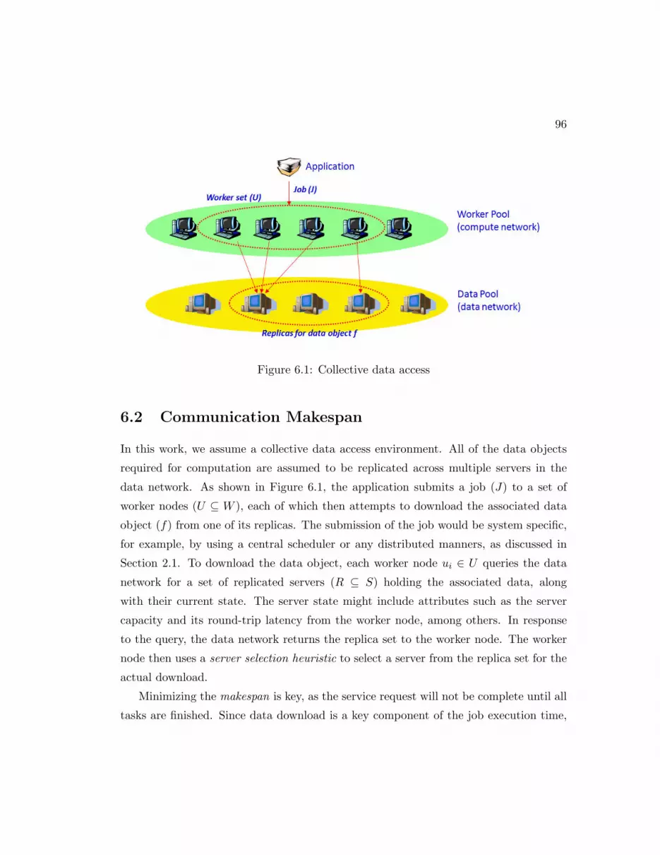
96
Figure 6.1: Collective data access
6.2 Communication Makespan
In this work, we assume a collective data access environment. All of the data objects
required for computation are assumed to be replicated across multiple servers in the
data network. As shown in Figure 6.1, the application submits a job (J) to a set of
worker nodes (U ⊆ W ), each of which then attempts to download the associated data
object (f) from one of its replicas. The submission of the job would be system specific,
for example, by using a central scheduler or any distributed manners, as discussed in
Section 2.1. To download the data object, each worker node ui ∈ U queries the data
network for a set of replicated servers (R ⊆ S) holding the associated data, along
with their current state. The server state might include attributes such as the server
capacity and its round-trip latency from the worker node, among others. In response
to the query, the data network returns the replica set to the worker node. The worker
node then uses a server selection heuristic to select a server from the replica set for the
actual download.
Minimizing the makespan is key, as the service request will not be complete until all
tasks are finished. Since data download is a key component of the job execution time,

97
Figure 6.2: Communication makespan
we define the communication makespan to be the maximal download time for job J :
makespan(J) = maxui∈U
(cost(ui, ri)), (6.1)
where ri is one of the replicated servers chosen by ui to download the data; i.e.,
ri ∈ R. Note that cost here is communication cost, as described in Section 2.1.
Figure 6.2 shows an example of the communication makespan. In this example,
four worker nodes need to download files for their computation work. Although worker
nodes A,B,C complete downloading early within 30 time units, the communication
makespan becomes 200 time units due to slow downloading by worker node D. This
one late communication could affect overall job completion, particularly for applications
relying on a collective performance metric.
The objective of this work is to reduce the communication makespan by selecting
“good” data servers. A challenge is that the individual compute workers are distributed
and isolated from each other. Collecting global state dynamically to improve server
selection is neither scalable nor practical. On the other hand, a greedy server selection
technique might choose the best server for each node locally without consideration of

98
1 3 5 7 100
10
20
30
40
50
60
70
80
Concurrency
Dow
nloa
d T
ime
(sec
onds
)
ksuvenustamuubcfluxwroc
Figure 6.3: Heterogeneity of servers
the other workers. Figure 6.3 shows how such a greedy approach might degrade the
download performance of servers by increasing the concurrency of downloads. This ex-
periment uses a set of PlanetLab nodes. Another point to be noted from this graph is
the heterogeneity of nodes in PlanetLab—each server has a different level of sensitivity
with respect to concurrent downloading requests, indicating the difference in their ca-
pacities. Our goal is to incorporate such server heterogeneity to do local server selection
while avoiding poor global decisions.
6.3 Server Selection Heuristics
In this section, we investigate different metrics that affect the efficiency of data down-
loading. Based on the impact of these metrics, we present heuristics for selecting data
servers in our environment. A key requirement of our model is to minimize the overall
makespan of a service request, and not to simply minimize the individual download
times at each worker independently.

99
To explore metrics that can potentially affect collective performance, we conducted
experiments with 43 nodes in PlanetLab to determine the various parameters that affect
download performance. An experimental evaluation was performed on PlanetLab over
a 7-month period (April–October, 2006). Several measures are explored, and we find
strong correlations not only between RTT and download performance, but also between
network bandwidth and download performance. RTT is gathered from our deployed
data network, Pastry [43], while Iperf [78] statistics are used to determine network
bandwidth. Figures 6.4(a) and 6.4(b) show the relationship of download times with RTT
and bandwidth, respectively. We use 4 different data download sizes: 256KB, 512KB,
1MB, and 2MB. Each point in these graphs corresponds to a single data download. We
make the following observations from these graphs:
• Observation 1: In the case of RTT (Figure 6.4(a)), the vast majority of data
download times for each data size are lower-bounded by a linear curve, indicating
the presence of a near-linear relationship to RTT. However, the variation in the
observed download times suggests the impact of other parameters.
• Observation 2: In the case of bandwidth (Figure 6.4(b)), we observe that the lower
bound on the download times for each data size has an exponential relationship to
bandwidth. In other words, servers with fairly large bandwidth (e.g., those over
10Mbps) do not show considerable difference among their download time trends,
while low bandwidth servers (e.g., those under 1Mbps) show a sharp increase in
the download time as the bandwidth decreases. However, again, the variation in
the observed download times suggests the impact of other parameters.
• Observation 3: We also observed that system load and concurrency are correlated
to download time (the effect of concurrency is illustrated in Figure 6.3)1 . These
factors may impact the performance if too many concurrent downloads occur
from the same server simultaneously. Such concurrency may happen due to race
conditions, where independent workers making independent download decisions
might select the same “desirable” server, in turn overloading it. Such overloading
should be avoided to minimize the communication makespan.
1 We did not find correlation to other parameters such as CPU power, size of memory, etc., in ourexperiments.

100
0 50 100 150 200 250 3000
5
10
15
20
25
RTT (msec)
Dow
nloa
d T
ime
(sec
)
256K512K1M2M
(a) Performance correlation with RTT
10−1
100
101
102
5
10
15
20
25
30
35
40
45
50
Bandwidth (Mbps)
Dow
nloa
d T
ime
(sec
)
256K512K1M2Mexp(0.8/bw)exp(1.0/bw)exp(1.2/bw)
(b) Performance correlation with bandwidth
Figure 6.4: Performance correlation between RTT and bandwidth

101
Based on these observations, we gain the following insights into making server se-
lection:
• Servers with low bandwidth (e.g., under 1Mbps) should be avoided, even if their
RTT is small.
• Servers with relatively high bandwidth (e.g., over 10Mbps) should be preferred,
and should use RTT as a discriminator.
• Servers with medium bandwidth (e.g., between 1–10Mbps) should be discrimi-
nated by load or concurrency.
We use these insights to derive a cost function that is used by a worker i to quantify
the desirability of a server j for data download:
cost(i, j) = αj · rtt(i, j), (6.2)
αj is a weight used to incorporate other server parameters, defined as follows:
αj = e(kj/bwj), (6.3)
where, bwj is the bandwidth of the server, and kj is a (server-dependent) constant that
incorporates parameters such as load and concurrency (discussed below).
This cost function has the following desired properties based on our observations.
First, the cost function is proportional to RTT (Observation 1), such that the pro-
portionality constant is the weight αj , which incorporates the effect of other server
parameters. Second, the cost function has an exponential relation to the server band-
width (Observation 2). Finally, we define the constant kj to incorporate factors, such
as load and concurrency (Observation 3). Note that the values returned by the cost
function are not meant to be absolute (i.e., these values are not used for predicting
the actual download times), but their relative values can be used for ranking multiple
servers in the order of their selection desirability.
We define three heuristics for server selection that use different values for kj :
• Bw-only: Uses kj = constant. We use kj = 1 in our experiments.
• Bw-load: Uses kj = loadj , where loadj is the 5-minute average system load on
the server.

102
Table 6.1: Experimental setupExperiments Nodes Replication Concurrency Data Size Number of Queries
EX-1 19 10 5 2M 690EX-2 33 10 5 256K,512K,1M,2M 547,274,490,233EX-3 29 10 5,10,15 2M 268,506,679EX-4 29 10 5 256K,512K,1M,2M 545, 572, 688, 472
• Bw-cand: Uses kj = num responsej , where num responsej is the number of
times the servers has responded as a replica server within the last 15 seconds.
The heuristic Bw-only uses only the RTT and the bandwidth metrics for selecting
a server, while the other heuristics Bw-load and Bw-cand also use average system
load and concurrency information, respectively. For Bw-load, we use a 5-minute sys-
tem load as the load metric, which is obtained by Linux uptime command. As the
load value grows, the weight becomes large, and the predicted download cost goes up.
Bw-cand uses the number of times the server has responded as a replica within a
predetermined time window. In the experiments, we set the time window to 15 sec-
onds, which is equal to the search time we used in the DHT ring. Using the heuristic
Bw-cand, servers that have responded as a replica several times recently are penal-
ized because they are more likely to be selected by multiple workers, and tend to be
concurrently serving data in the near future.
Again, these heuristics are not for individual performance, but for collective perfor-
mance. Recall that our efforts in the previous chapters focus on improving individual
performance. That is why the BW-class heuristics in this chapter incorporate server-side
properties for local server selection.
6.4 Performance Evaluation
6.4.1 Experimental Testbed and Methodology
To evaluate the various server selection heuristics described in the previous section,
we conducted experiments on a set of randomly selected PlanetLab nodes geographi-
cally distributed across the globe: North America 20, Europe 19, and Asia/Pacific 4

103
Figure 6.5: Procedure for server selection and data download
nodes. For data replication and download, we implemented a data network over FreeP-
astry [109], a public Pastry implementation developed by Rice University. FreePastry
provides the underlying data placement, request and data routing mechanisms.
We conducted each of our experiments as follows: data files are distributed over the
data network at the beginning of each experiment, and then data queries are generated
for downloading these data files. For each data query, a set of worker nodes are selected
randomly to request the same designated file concurrently. For fair comparison across
the different server selection heuristics, queries are interleaved: e.g., each set of worker
nodes downloads the files first with the Proxim (latency-based heuristic) selection,
followed by the Bw-only selection, etc. Some queries might fail due to reasons such
as churn (e.g., nodes going down) or query incompletion (e.g., message routing failure in
the DHT ring). If any query fails in the interleaved set of queries, the result is discarded
in our analysis.

104
Figure 6.5 illustrates the procedure for server selection and data download at each
worker node: (1) a worker node sends a search query to obtain the list of replica servers
for the data to retrieve; (2) the root data server responsible for the data returns a list of
replica servers; and (3) the worker node chooses a replica server from the list based on
the selection algorithm and downloads the data from the selected replica server. After
completing the download, the elapsed time is recorded for comparison.
There are two main parameters that we vary across our experiments: (i) data down-
load size, with values of 256KB, 512KB, 1MB, and 2MB; and (ii) concurrency of client
access for the same file, using values of 5, 10, and 15. We use a replication factor of 10
for placing each data file to provide us with a relatively large set of replica servers for
download. This allows a better comparison of server selection heuristics. In addition,
we use different sets of machines in each experiment, with randomly chosen data place-
ment (driven by FreePastry) to generate different environmental conditions. Table 6.1
shows the various experimental scenarios we created. The scenarios differ in some of
the parameters above, as well as the specific set and number of nodes that were used.
6.4.2 Comparison of Server Selection Heuristics
Figure 6.6 compares the server selection heuristics for concurrency=5 and data=2MB,
using the aggregated results of all the experiments that used the same concurrency
and data size. The figure plots the average download time and makespan respectively
for the various heuristics. The first observation we make from the figure is that the
bandwidth-based heuristics perform much better that latency-based server selection in
terms of both the average, as well as the makespan. In the figure, we can see that the
gaps in performance are greater in the case of the makespan (∼30–45%) than in the
mean download time (∼20–30%).
This result is also seen from Figure 6.7 that plots the cumulative distribution of
the download completion times. As seen from the figure, 10% of Proxim queries take
more than 60 seconds to complete, while the bandwidth-based heuristics take less than
40 seconds to complete 90% of their queries. Moreover, these heuristics finish most of
their queries within approximately 100 seconds, while nearly 5% percent of queries are
unfinished for Proxim selection. Thus, this result implies that using bandwidth in ad-
dition to latency produces better performance, not only in terms of individual download,

105
Average Makespan0
5
10
15
20
25
30
35
40
Dow
nloa
d T
ime
(sec
onds
)
PROXIMBW−ONLYBW−LOADBW−CAND
Figure 6.6: Performance comparison (concurrency=5, data=2MB)
but also in the overall makespan.
Another observation we make from Figures 6.6 and 6.7 is that Bw-cand shows
the best results for both the mean download time and makespan. In the case of the
makespan, Bw-cand gains over 40% compared to Proxim, while Bw-only and
Bw-load show 30–40% gains. Figure 6.7 shows the CDF of the completion times
of all the queries. This result implies that incorporating concurrency in addition to
bandwidth improves the performance even further.
While Figure 6.6 shows the aggregated results, Figure 6.9 depicts the results sep-
arately for each experiment. Once again, we see that bandwidth-based heuristics out-
perform latency-based server selection in all cases, and that Bw-cand performs best
in all cases (except EX-2, where its performance is equivalent to the other heuristics).
The basic reason why the bandwidth-based heuristics outperform latency-based se-
lection is that they can exclude extremely slow servers. In our experiments, the partici-
pating hosts are almost uniformly distributed through the bandwidth ranges, as shown
in Figure 6.8: nearly 10% of the hosts have a bandwidth under 1Mbps; 50% of the hosts

106
0 20 40 60 80 100 120 140 160 1800
0.1
0.2
0.3
0.4
0.5
0.6
0.7
0.8
0.9
1
Makespan (seconds)
Fra
ctio
n of
que
ries
Makespan CDF
PROXIMBW−ONLYBW−LOADBW−CAND
Figure 6.7: Cumulative distribution of download completion times
have under 30Mbps, and the upper 10% hosts have over 80Mbps bandwidth. By penal-
izing low bandwidth servers, bandwidth-based heuristics can select servers with better
bandwidth, even though they may be a little further from the worker node. Given that
PlanetLab systems are well-organized compared to systems in typically large-scale in-
frastructures, we anticipate that the heuristics can differentiate the results much more
in such environments.
Table 6.2: Server bandwidth distributionClass Low Medium High
< 1Mbps 1− 10Mbps > 10Mbps
EX-1 5% 26% 67%EX-2 12% 6% 82%EX-3 0% 24% 76%EX-4 0% 24% 76%

107
10−1
100
101
102
0
0.1
0.2
0.3
0.4
0.5
0.6
0.7
0.8
0.9
1
Bandwidth (Mbps)
Fra
ctio
n
Host Bandwidth CDF (log scale)
Figure 6.8: Bandwidth distribution of data servers
The reason Bw-cand performs the best can be found in the bandwidth distribu-
tion of servers, as shown in Table 6.2. Here, we classify hosts in three categories: low,
medium, and high bandwidth, based on their bandwidth values. All of the bandwidth-
based heuristics can penalize low-bandwidth servers (i.e., those with less than 1Mbps),
but may not penalize medium-bandwidth servers (i.e., those between 1Mbps and 10Mbps).
In fact, Bw-only might not penalize such medium-class servers because the weight
value αj is likely to stabilize beyond 1Mbps, due to its exponential relation to band-
width (Equation 6.3). In addition, if the average load is low on these medium-class
hosts (close to 1), Bw-load also does not penalize them. In contrast, Bw-cand can
penalize these servers if too many clients try to select them, thus leading to higher values
of recent replica set queries. Thus, Bw-cand is able to provide better performance
for such servers by proactively preventing overloads from happening, while Bw-load
is able to react only to past observed load. Unlike other experiments, EX-2 shows all
heuristics to have similar performance. This can be explained by the fact that EX-2
has only 6% medium-class servers (as seen from Table 6.2), whereas other experimental
scenarios have more than 20% medium-class servers, thus reducing the differentiation

108
EX−1 EX−2 EX−3 EX−40
10
20
30
40
50
60
Mak
espa
n (s
econ
ds)
PROXIMBW−ONLYBW−LOADBW−CAND
Figure 6.9: Performance of individual experiments (concurrency=5, data=2MB)
opportunity for Bw-cand. However, note that Bw-cand does not perform any worse
than other heuristics, even under these conditions.
6.4.3 Impact of Data Size
Figure 6.10 shows the average makespan obtained for varying data sizes from 256KB
to 2MB in EX-2 and EX-4. Figure 6.10(a) shows that the bandwidth-based heuristics
outperform latency-based selection much more significantly as the data size increases,
going from 16% for 256KB to 42% for 2MB when comparing Bw-cand to Proxim.
Another experiment in Figure 6.10(b) shows similar results, making it greater the gap
between Proxim and our heuristics as data size increases. This result indicates that
while latency-based selection may be sufficient for small data sizes, server bandwidth
assumes an important role for larger data sizes.

109
256KB 512KB 1MB 2MB0
5
10
15
20
25
30
35
40
45
50
Mak
espa
n (s
econ
ds)
PROXIMBW−ONLYBW−LOADBW−CAND
(a) EX-2
256KB 512KB 1MB 2MB0
5
10
15
20
25
30
35
40
45
50
Mak
espa
n (s
econ
ds)
PROXIMBW−ONLYBW−LOADBW−CAND
(b) EX-4
Figure 6.10: Impact of data size (EX-2 and EX-4; concurrency=5, data=All)

110
5 10 150
10
20
30
40
50
60
70
80
90
Concurrency
Mak
espa
n (s
econ
ds)
PROXIMBW−ONLYBW−LOADBW−CAND
Figure 6.11: Impact of concurrency (EX-3; data=2MB)
6.4.4 Impact of Concurrency
To see the impact of concurrent downloads for the same files, we used concurrency
values of 10 and 15 in addition to the value of 5 used in our previous experiments.
Since the replication factor for data placement is set to 10, race conditions would be
unavoidable in this experiment with clients selecting the same server for download in
several cases. Figure 6.11 shows the experimental results in such diverse concurrent
downloading environments. In the figure, we can see that the bandwidth-based heuris-
tics consistently outperform latency-based techniques. Moreover, we see that as the
concurrency increases, Bw-cand starts outperforming the other heuristics, indicating
that avoiding overloads by reducing concurrent data downloads from the same server is
important.

111
6.5 Summary
In this work, we focused on the server selection problem in collective data access envi-
ronments: how do individual nodes select a server for downloading data to minimize the
communication makespan—the maximal download time for a data file? The commu-
nication makespan is an important measure because the successful completion of jobs
is driven by the efficiency of collective data download across compute nodes, and not
only the individual download times. Through experiments conducted on a Pastry net-
work running on PlanetLab, we showed that conventional latency-based server selection
does not always produce good results. We demonstrated that nodes in a distributed
system are heterogeneous in terms of several metrics, such as bandwidth, load, and
capacity, which further impact their download behavior. We proposed new server se-
lection heuristics that incorporate these metrics, namely, the server bandwidth, load,
and download concurrency, and showed that these heuristics outperform latency-based
server selection, reducing average makespans by at least 30%. We further showed that
incorporating information about download concurrency avoids overloading servers, and
improves performance by approximately 17–43% over heuristics considering only latency
and bandwidth.

Chapter 7
Conclusion and Future Directions
In this chapter, we provide concluding remarks and future research directions.
7.1 Conclusion
Large-scale distributed systems are attractive with the virtues of scalability and cost-
effectiveness. However, major challenges in such systems are network unpredictability
and limited bandwidth available for data dissemination. Emerging scientific applica-
tions, however, are data-intensive and require access to a significant amount of dispersed
data. For such applications, performance depends critically on efficient data delivery
to computational nodes. Moreover, the efficiency of data delivery for such applications
would critically depend on the location of data and the points of access. Hence, in order
to accommodate data-intensive applications in large-scale platforms, it is essential to
consider not only the computational capability, but also the data accessibility of compu-
tational nodes to the required data objects. This thesis explored how we could provide
predictability in data access for data-intensive computing in large-scale computational
infrastructures in which nodes are highly heterogeneous and bandwidth is expensive.
Our primary effort for predictability in data access is to develop the OPEN frame-
work to provide end-to-end network performance estimation. In Chapter 3, we showed
how we could make accurate estimations with past data access information without
expensive on-demand probing. The key idea in this work is to characterize nodes based
112
113
on their past, local downloading measurements. In self-estimation, the node makes es-
timation based on its characterized value and distance to the server. Another technique
called neighbor estimation utilizes neighbors’ measurements in addition to the character-
ized value of itself. This technique, in particular, enables nodes to share measurements
without any geographical or topological restrictions.
Based on our neighbor estimation technique in Chapter 3, we constructed the OPEN
framework in Chapter 4. First, we extended neighbor estimation to topology-free, pas-
sive estimation as a generalization. Then, we developed algorithms for efficient dis-
semination of measurements in order to make historical measured information globally
visible, so that nodes can make their own estimation, based on such shared informa-
tion in addition to their local measurements. The dissemination algorithms are based
on information criticality; i.e., how critical is the information to the system. With
gossip-based probabilistic dissemination, the optimizations dramatically diminish dis-
semination overheads without significant performance loss.
These two blocks of work, passive estimation and proactive dissemination, are the
basis of the OPEN framework. The framework is indeed scalable, decentralized, and
topology-neutral in providing end-to-end network performance. Moreover, OPEN is
sufficiently accurate in offering a meaningful rank order of nodes, based on network
performance.
In Chapter 5, we considered parallel data access environments in which multiple
replicated servers can be utilized in parallel when downloading a single data file. In this
body of work, we consider two problems: (1) how we can utilize multiple servers in par-
allel; and (2) how we can make resource selection in such parallel environments. We ob-
served that greedy-based data access is adaptable in utilizing multiple servers; however,
we also observed that any slowdown can prolong the completion of data downloading,
thereby offsetting the benefits of parallelism. Our optimization that uses redundancy
to mask failure or slowdown of late blocks can effectively handle those unpredictable
situations, thus significantly improving both performance and fault tolerance. In ad-
dition, we address the problem of resource selection to identify good resources for job
allocation under such parallel data access environments, and show that simple addition
of historical node download information can improve the quality of resource selections.
The last block in this thesis is collective data access for applications for which group

114
performance is more important than individual performance, as discussed in Chapter 6.
To minimize communication makespan, a quantitative metric for group performance, we
presented server selection heuristics that incorporate several end-to-end and server-side
metrics, including latency, bandwidth, server load, and capacity. Through live exper-
iments in PlanetLab, the results show that incorporating information about download
concurrency avoids overloading servers.
7.2 Future Directions
7.2.1 Supporting Cluster-structured Grids
OPEN will ideally fit large-scale desktop grids harnessing idle cycles. We further be-
lieve that our framework can be applied to existing grid systems having a multi-site,
cluster-based architecture, since we made no assumptions about topological constraints.
Figure 7.1 shows a grid system with 3 virtual organizations in which computational or
data resources are located. In such an environment, secondhand measurements from
nodes in the same virtual organization (or cluster) can be given more weight in the
estimation process. One of the future research directions is to optimize our OPEN
framework to better support such cluster-based, large-scale systems.
7.2.2 Improving Estimation Accuracy
Intrinsically, firsthand measurement-based estimation would be more accurate than sec-
ondhand measurement-based techniques. Figure 7.2 compares relative errors of estima-
tions for two estimation approaches. Although our secondhand technique works quite
well, locating ∼ 90% of the total estimations within a factor of 2, it is still behind
the firsthand technique, based on the mean. The main reason that pairwise techniques
perform worse in Chapter 4 is due to the shortage of relevant measures because they
require O(n2) measures, at worst. Since we target large-scale distributed systems, con-
sulting secondhand measures is definitely attractive. However, it is possible to consider
a combination of the pairwise techniques to the OPEN framework to exploit pairwise
measures, if any. We believe that this is one of our future projects to improve the
accuracy of OPEN estimation.

115
Figure 7.1: A grid system
0 0.5 1 1.5 2 2.5 3 3.5 40
0.1
0.2
0.3
0.4
0.5
0.6
0.7
0.8
0.9
1
Relative error
Cum
ulat
ive
frac
tion
Comparison of estimation techniques (# observation=8, Data=Mix)
firsthandsecondhand
Figure 7.2: Estimation accuracy

116
In addition, utilizing outdated measurements can adversely affect estimation accu-
racy. To determine the staleness of measurements, we could use a timestamp. If the
aging-out time interval is too big, estimation takes place with stale information, caus-
ing inaccuracy. If too short, estimation failure rate will increase, due to a shortage of
measurements. The SPAND authors [60] observed that aggregating past measurements
for 5 hours is still valid for performance prediction, despite traffic changes of the day
in their experiments. However, it may be different between systems. Moreover, large
systems may have different characteristics from a single network. Our future efforts will
include a thorough investigation of determining staleness for measurements.
7.2.3 Optimizing Dissemination
OPEN employs gossip techniques for cost-effective dissemination of measurements. Typ-
ically, gossip techniques rely on gossip probability (or dissemination probability), which
can be chosen to meet application-specific goals, such as dissemination completion rates
(i.e., the fraction of nodes that successfully received dissemination messages) and dissem-
ination overhead (i.e., the number of dissemination messages or bandwidth consumption
by dissemination). A critical challenge here is how to determine gossip probability to
meet such user goals. For example, different dissemination completion rates can be
possible in different systems, despite using the same gossip probability.
Figure 7.3 shows how gossip probability impacts three different systems with dis-
tinct node degrees, i.e., the number of neighbors with minimum and maximum sizes.
In the figure, the x-axis represents dissemination probability, and the y-axis represents
the fraction of nodes that successfully received dissemination messages. As seen in the
figure, node degree has a considerable impact on the dissemination completion rate. If
the system has a fixed node degree, we may be able to precompute the gossip proba-
bility and globally configure it. Even in this case, however, the chosen probability may
not properly work, due to some reasons, such as the dynamics of distributed systems.
SmartGossip [86] addresses this problem by learning local topology. However, it assumes
a broadcasting environment in sensor networks, and there may be different problems
to be addressed for large-scale distributed systems. One of our future directions is to
explore dissemination parameters and conditions to achieve various application goals
rather than to rely on fixed global configurations in large-scale settings.

117
0 0.2 0.4 0.6 0.8 10
0.1
0.2
0.3
0.4
0.5
0.6
0.7
0.8
0.9
1
Dissemination probability
Fra
ctio
n of
nod
es
Impact of system degree (# nodes=10000)
degree=2−6degree=4−12degree=8−16
Figure 7.3: Impact of node degree and dissemination probability
7.2.4 Developing Scheduling Algorithms for Parallelism
Parallelism is appealing due to both performance and fault tolerance. Besides our efforts
for parallel data access, there still would be many interesting challenges for future
exploration. In the greedy-based data access we proposed, one interesting question
involves which block should be assigned for redundant access. Different optimizations
exist, including old-block-first and latest-block-first, to name a few. We plan to examine
a rich set of scheduling techniques for this question.
7.2.5 Capturing Availability
The accessibility metric currently considers performance, but our future work will con-
sider capturing both performance and availability. Even if we expect high performance
to access a server by estimation, the server could be unavailable at a specific time frame,
due to node churn or overloading. If our accessibility metric captures availability as well
as performance, it will be possible to make better selections, thereby reducing potential
failures or slowdowns in accessing servers.

Bibliography
[1] Jinoh Kim, Abhishek Chandra, and Jon B. Weissman. Accessibility-based re-
source selection in loosely-coupled distributed systems. In Proceedings of 28th
International Conference on Distributed Computing Systems (ICDCS ’08), pages
777–784, 2008.
[2] Jinoh Kim, Abhishek Chandra, and Jon B. Weissman. Using data accessibility
for resource selection in large-scale distributed systems. IEEE Transactions on
Parallel and Distributed Systems, 20(6):788–801, 2009.
[3] Jinoh Kim, Abhishek Chandra, and Jon B. Weissman. Exploiting heterogeneity
for collective data downloading in volunteer-based networks. In Proceedings of the
2007 Seventh IEEE International Symposium on Cluster Computing and the Grid
(CCGRID ’07), pages 275–282, 2007.
[4] Climateprediction.net: http://www.climateprediction.net.
[5] N. Massey, T. Aina, M. Allen, C. Christensen, D. Frame, D. Goodman, J. Ket-
tleborough, A. Martin, S. Pascoe, and D. Stainforth. Data access and analysis
with distributed federated data servers in climateprediction.net. Advances in Geo-
sciences, 8:49–56, June 2006.
[6] Carl Christensen, Tolu Aina, and David Stainforth. The challenge of volun-
teer computing with lengthy climate model simulations. In Proceedings of E-
SCIENCE, pages 8–15, 2005.
[7] IrisNet: http://www.intel-iris.net/index.html.
118

119
[8] Phillip B. Gibbons, Brad Karp, Yan Ke, Suman Nath, and Srinivasan Seshan.
Irisnet: An architecture for a worldwide sensor web. IEEE Pervasive Computing,
2(4):22–33, 2003.
[9] PPDG: Particle physics data grid, http://www.ppdg.net.
[10] G. B. Berriman, A. C. Laity, J. C. Good, J. C. Jacob, D. S. Katz, E. Deelman,
G. Singh, M.-H. Su, and T. A. Prince. Montage: The architecture and scientific
applications of a national virtual observatory service for computing astronomical
image mosaics. In Proceedings of Earth Sciences Technology Conference, 2006.
[11] BLAST: The basic local alignment search tool,
http://www.ncbi.nlm.nih.gov/blast.
[12] Bill Allcock, Joe Bester, John Bresnahan, Ann L. Chervenak, Ian Foster, Carl
Kesselman, Sam Meder, Veronika Nefedova, Darcy Quesnel, and Steven Tuecke.
Data management and transfer in high-performance computational grid environ-
ments. Parallel Computing, 28(5):749–771, 2002.
[13] Wolfgang Hoschek, Francisco Javier Jaen-Martınez, Asad Samar, Heinz
Stockinger, and Kurt Stockinger. Data management in an international data
grid project. In Proceedings of GRID (GRID ’00), pages 77–90, 2000.
[14] Yong-Meng Teo, Xianbing Wang, and Yew-Kwong Ng. Glad: a system for develop-
ing and deploying large-scale bioinformatics grid. Bioinformatics, 21(6):794–802,
2005.
[15] David P. Anderson. BOINC: A system for public-resource computing and storage.
In Proceedings of GRID (GRID ’04), pages 4–10, 2004.
[16] Virginia Lo, Daniel Zappala, Dayi Zhou, Yuhong Liu, and Shanyu Zhao. Cluster
computing on the fly: P2p scheduling of idle cycles in the internet. In Proceedings
of the IEEE Fourth International Conference on Peer-to-Peer Systems, pages 227–
236, 2004.
[17] Andreas Haeberlen, Alan Mislove, and Peter Druschel. Glacier: Highly durable,
decentralized storage despite massive correlated failures. In Proceedings of

120
USENIX Symposium on Networked Systems Design and Implementation (NSDI
’05), May 2005.
[18] John Kubiatowicz, David Bindel, Yan Chen, Patrick Eaton, Dennis Geels, Ra-
makrishna Gummadi, Sean Rhea, Hakim Weatherspoon, Westly Weimer, Christo-
pher Wells, and Ben Zhao. Oceanstore: An architecture for global-scale persistent
storage. In Proceedings of ACM ASPLOS, November 2000.
[19] Ranjita Bhagwan, Kiran Tati, Yu-Chung Cheng, Stefan Savage, and Geoffrey M.
Voelker. Total recall: system support for automated availability management. In
Proceedings of USENIX Symposium on Networked Systems Design and Implemen-
tation (NSDI ’04), pages 25–25, 2004.
[20] P. Druschel and A. Rowstron. PAST: A large-scale, persistent peer-to-peer storage
utility. In HotOS VIII, pages 75–80, May 2001.
[21] Douglas Thain, Todd Tannenbaum, and Miron Livny. Distributed computing in
practice: the condor experience. Concurrency - Practice and Experience, 17(2-
4):323–356, 2005.
[22] The Globus Alliance, http://www.globus.org/.
[23] Derrick Kondo, Andrew A. Chien, and Henri Casanova. Resource management
for rapid application turnaround on enterprise desktop grids. In Proceedings of
the 2004 ACM/IEEE conference on Supercomputing (SC ’04), 2004.
[24] Gilles Fedak, Haiwu He, and Franck Cappello. Bitdew: a programmable envi-
ronment for large-scale data management and distribution. In Proceedings of the
2008 ACM/IEEE conference on Supercomputing (SC ’08), 2008.
[25] Andrew Chien, Brad Calder, Stephen Elbert, and Karan Bhatia. Entropia: archi-
tecture and performance of an enterprise desktop grid system. Journal of Parallel
and Distributed Computing, 63(5):597–610, 2003.
[26] Amazon elastic compute cloud (ec2): http://aws.amazon.com/ec2/.
[27] Windows azure platform: http://www.microsoft.com/windowsazure/.

121
[28] Magellan nersc cloud testbed: http://www.nersc.gov/nusers/systems/magellan/.
[29] David P. Anderson, Jeff Cobb, Eric Korpela, Matt Lebofsky, and Dan Werthimer.
Seti@home: an experiment in public-resource computing. Communications of the
ACM, 45(11):56–61, 2002.
[30] Search for extraterrestrial intelligence (SETI) project,
http://setiathome.berkeley.edu.
[31] Folding@home disributed computing, http://folding.stanford.edu/.
[32] Einstein@home, http://www.einsteinathome.org/.
[33] BOINC: Berkeley open infrastructure for network computing,
http://boinc.berkeley.edu/.
[34] David P. Anderson and Gilles Fedak. The computational and storage potential of
volunteer computing. In Proceedings of the Sixth IEEE International Symposium
on Cluster Computing and the Grid (CCGRID ’06), pages 73–80, 2006.
[35] Nicolas Kourtellis, Lydia Prieto, Adriana Iamnitchi, Gustavo Zarrate, and Dan
Fraser. Data transfers in the grid: workload analysis of globus gridftp. In Pro-
ceedings of the 2008 international workshop on Data-aware distributed computing
(DADC ’08), pages 29–38, 2008.
[36] PlanetLab, http://www.planet-lab.org.
[37] Larry Peterson, Andy Bavier, Marc E. Fiuczynski, and Steve Muir. Experiences
building planetlab. In Proceedings of the 7th USENIX Symposium on Operating
Systems Design and Implementation (OSDI ’06), 2006.
[38] Planetlab traces: http://ridge.cs.umn.edu/pltraces.html.
[39] Edith Cohen and Scott Shenker. Replication strategies in unstructured peer-
to-peer networks. In Proceedings of ACM SIGCOMM (SIGCOMM ’02), pages
177–190, 2002.

122
[40] Qin Lv, Pei Cao, Edith Cohen, Kai Li, and Scott Shenker. Search and replication
in unstructured peer-to-peer networks. In Proceedings of ACM SIGMETRICS
(SIGMETRICS ’02), pages 258–259, 2002.
[41] Ion Stoica, Robert Morris, David Karger, M. Frans Kaashoek, and Hari Balakr-
ishnan. Chord: A scalable peer-to-peer lookup service for internet applications.
In Proceedings of ACM SIGCOMM (SIGCOMM ’01), pages 149–160, 2001.
[42] Sylvia Ratnasamy, Paul Francis, Mark Handley, Richard Karp, and Scott
Schenker. A scalable content-addressable network. In Proceedings of ACM SIG-
COMM (SIGCOMM ’01), pages 161–172, 2001.
[43] Antony Rowstron and Peter Druschel. Pastry: Scalable, distributed object lo-
cation and routing for large-scale peer-to-peer systems. In IFIP/ACM Interna-
tional Conference on Distributed Systems Platforms (Middleware), pages 329–350,
November 2001.
[44] B. Zhao, L. Huang, J. Stribling, S. Rhea, A. Joseph, and J. Kubiatowicz. Tapestry:
A resilient global-scale overlay for service deployment. In IEEE Journal on Se-
lected Areas in Communications, 2003.
[45] R. Raman, M. Livny, and M. Solomon. Matchmaking: Distributed resource man-
agement for high throughput computing. In Proceedings of Proceedings of ACM
High Performance Distributed Computing (HPDC ’98), page 140, 1998.
[46] D. Oppenheimer, J. Albrecht, D. Patterson, and A. Vahdat. Design and imple-
mentation tradeoffs for wide-area resource discovery. In Proceedings of Proceedings
of ACM High Performance Distributed Computing (HPDC ’05), 2005.
[47] D. Zhou and V. Lo. Cluster computing on the fly: resource discovery in a cycle
sharing peer-to-peer system. In Proceedings of the 2004 Fourth IEEE International
Symposium on Cluster Computing and the Grid (CCGRID ’04), pages 66–73,
2004.
[48] Michael Cardosa and Abhishek Chandra. Resource bundles: Using aggregation
for statistical wide-area resource discovery and allocation. In Proceedings of 28th

123
International Conference on Distributed Computing Systems (ICDCS ’08), pages
760–768, 2008.
[49] Jik-Soo Kim, Beomseok Nam, Peter Keleher, Michael Marsh, Bobby Bhattachar-
jee, and Alan Sussman. Resource discovery techniques in distributed desktop grid
environments. In Proceedings of GRID (GRID ’06), September 2006.
[50] William Allcock, John Bresnahan, Rajkumar Kettimuthu, and Michael Link. The
globus striped gridftp framework and server. In Proceedings of ACM/IEEE Con-
ference on Supercomputing (SC ’05), 2005.
[51] B. Cohen. Incentives build robustness in bittorrent. In Workshop on Economics
of Peer-to-Peer Systems, 2003.
[52] Bittorrent, http://www.bittorrent.com/.
[53] Baohua Wei, G. Fedak, and F. Cappello. Scheduling independent tasks sharing
large data distributed with bittorrent. In Proceedings of the 6th IEEE/ACM
International Workshop on Grid Computing (GRID ’05), 2005.
[54] Fernando Costa, Luis Silva, Gilles Fedak, and Ian Kelley. Optimizing the data
distribution layer of boinc with bittorrent. In Proceedings of the Second Workshop
on Desktop Grids and Volunteer Computing held in conjunction with IPDPS 2008
(PCGRID 2008), 2008.
[55] Haiwu He, Gilles Fedak, Bing Tang, and Franck Cappello. Blast application with
data-aware desktop grid middleware. In Proceedings of the 2009 9th IEEE/ACM
International Symposium on Cluster Computing and the Grid (CCGRID ’09),
pages 284–291, 2009.
[56] Gaurav Khanna 0002, Umit V. Catalyurek, Tahsin M. Kurc, P. Sadayappan, and
Joel H. Saltz. Scheduling file transfers for data-intensive jobs on heterogeneous
clusters. In Euro-Par, pages 214–223, 2007.
[57] Jun Feng and Marty Humphrey. Eliminating replica selection - using multiple
replicas to accelerate data transfer on grids. In Proceedings of International Con-
ference on Parallel and Distributed Systems (ICPADS ’04), 2004.
124
[58] T. S. Eugene Ng, Yang hua Chu, Sanjay G. Rao, Kunwadee Sripanidkulchai,
and Hui Zhang. Measurement-based optimization techniques for bandwidth-
demanding peer-to-peer systems. In Proceedings of INFOCOM (INFOCOM ’03),
pages 2199–2209, 2003.
[59] L.A. Barchet-Steffenel and G. Mounie. Scheduling heuristics for efficient broadcast
operations on grid environments. In Proceedings of IEEE International Parallel
and Distributed Processing Symposium (IPDPS ’06), 2006.
[60] S. Seshan, M. Stemm, and R. H Katz. SPAND: Shared Passive Network Perfor-
mance Discovery. In Proceedings of the USENIX Symposium on Internet Tech-
nologies and Systems, pages 135–146, Monterey, CA, December 1997.
[61] Matthew Andrews, Bruce Shepherd, Aravind Srinivasan, Peter Winkler, and Fran-
cis Zane. Clustering and server selection using passive monitoring. In Proceedings
of INFOCOM (INFOCOM ’02), pages 1717–1725, 2002.
[62] Sandra G. Dykes, Kay A. Robbins, and Clinton L. Jeffery. An empirical eval-
uation of client-side server selection algorithms. In Proceedings of INFOCOM
(INFOCOM ’00), pages 1361–1370, 2000.
[63] Ellen W. Zegura, Mostafa H. Ammar, Zongming Fei, and Samrat Bhattachar-
jee. Application-layer anycasting: a server selection architecture and use in a
replicated web service. IEEE/ACM Transactions on Networking, 8(4):455–466,
2000.
[64] Sudharshan Vazhkudai, Steven Tuecke, and Ian Foster. Replica selection in the
globus data grid. In Proceedings of the 1st International Symposium on Cluster
Computing and the Grid (CCGRID ’01), page 106, 2001.
[65] Robert L. Carter and Mark Crovella. Server selection using dynamic path charac-
terization in wide-area networks. In Proceedings of INFOCOM (INFOCOM ’97),
pages 1014–1021, 1997.
[66] Tina Tyan. A case study of server selection. Master’s thesis, Massachusetts
Institute of Technology, September 2001.

125
[67] Kevin Lai and Mary Baker. Nettimer: a tool for measuring bottleneck link, band-
width. In Proceedings of the 3rd conference on USENIX Symposium on Internet
Technologies and Systems (USITS’01), pages 11–11, 2001.
[68] R. Wolski, N. Spring, and J. Hayes. The Network Weather Service: A Distributed
Resource Performance Forecasting Service for Metacomputing. Journal of Future
Generation Computing Systems, 15:757–768, 1999.
[69] David Oppenheimer, Jeannie Albrecht, David Patterson, and Amin Vahdat. Scal-
able Wide-Area Resource Discovery. Technical report, University of California,
Berkeley UCB//CSD-04-1334, July 2004.
[70] Frank Dabek, Russ Cox, Frans Kaashoek, and Robert Morris. Vivaldi: a decentral-
ized network coordinate system. In Proceedings of ACM SIGCOMM (SIGCOMM
’04), pages 15–26, 2004.
[71] Paul Francis, Sugih Jamin, Cheng Jin, Yixin Jin, Danny Raz, Yuval Shavitt,
and Lixia Zhang. Idmaps: a global internet host distance estimation service.
IEEE/ACM Transactions on Networking, 9(5):525–540, 2001.
[72] E. Ng and H. Zhang. Predicting internet network distance with coordiantes-based
approaches. In Proceedings of IEEE INFOCOM (INFOCOM ’02), pages 170–179,
2002.
[73] Bernard Wong, Aleksandrs Slivkins, and Emin Gun Sirer. Meridian: a lightweight
network location service without virtual coordinates. SIGCOMM Computer Com-
munication Reviews, 35(4):85–96, 2005.
[74] M. Costa, M. Castro, A. Rowstron, and P. Key. Pic: Practical internet coordinates
for distance estimation. In International Conference on Distributed Systems, 2004.
[75] Allen B. Downey. Using pathchar to estimate internet link characteristics. In
Proceedings of ACM SIGCOMM (SIGCOMM ’99), pages 241–250, 1999.
[76] Srinivasan Keshav. Packet-pair flow control. IEEE/ACM Transactions on Net-
working, 1995.

126
[77] Qi He, Constantine Dovrolis, and Mostafa Ammar. On the predictability of large
transfer tcp throughput. In Proceedings of ACM SIGCOMM (SIGCOMM ’05),
pages 145–156, 2005.
[78] PlanetLab Iperf, http://www.measurement-lab.org/logs/iperf/.
[79] Rich Wolski. Experiences with predicting resource performance on-line in compu-
tational grid settings. SIGMETRICS Performance Evaluation Reviews, 30(4):41–
49, 2003.
[80] Harsha V. Madhyastha, Tomas Isdal, Michael Piatek, Colin Dixon, Thomas An-
derson, Arvind Krishnamurthy, and Arun Venkataramani. iPlane: An information
plane for distributed services. In Proceedings of the 7th USENIX Symposium on
Operating Systems Design and Implementation (OSDI ’06), 2006.
[81] Harsha V. Madhyastha, Ethan Katz-Bassett, Thomas Anderson, Arvind Krishna-
murthy, and Arun Venkataramani. iplane nano: path prediction for peer-to-peer
applications. In Proceedings of the 6th USENIX symposium on Networked systems
design and implementation (NSDI’09), pages 137–152, 2009.
[82] Anne-Marie Kermarrec, Laurent Massoulie, and Ayalvadi J. Ganesh. Probabilistic
reliable dissemination in large-scale systems. IEEE Transactions on Parallel and
Distributed Systems, 14(3):248–258, 2003.
[83] Spyros Voulgaris and Maarten van Steen. Hybrid dissemination: adding deter-
minism to probabilistic multicasting in large-scale p2p systems. pages 389–409,
2007.
[84] Mayur Deshpande, Bo Xing, Iosif Lazardis, Bijit Hore, Nalini Venkatasubrama-
nian, and Sharad Mehrotra. Crew: A gossip-based flash-dissemination system. In
Proceedings of the 26th IEEE International Conference on Distributed Computing
Systems (ICDCS ’06), page 45, 2006.
[85] Zygmunt J. Haas, Joseph Y. Halpern, and Li Li. Gossip-based ad hoc routing.
IEEE/ACM Transactions on Networking, 14(3):479–491, 2006.

127
[86] Pradeep Kyasanur, Romit Choudhury, and Indranil Gupta. Smart gossip: An
adaptive gossip-based broadcasting service for sensor networks. IEEE Interna-
tional Conference on Mobile Adhoc and Sensor Systems Conference, 0:91–100,
2006.
[87] A. Chervenak, I. Foster, C. Kesselman, C. Salisbury, and S. Tuecke. The
Data Grid: Towards an architecture for the distributed management and anal-
ysis of large scientific datasets. Journal of Network and Computer Applications,
23(3):187–200, 2000.
[88] Kavitha Ranganathan and Ian Foster. Decoupling computation and data schedul-
ing in distributed data-intensive applications. In Proceedings of ACM High Per-
formance Distributed Computing (HPDC ’02), page 352, 2002.
[89] Srikumar Venugopal, Rajkumar Buyya, and Lyle Winton. A grid service broker for
scheduling e-science applications on global data grids: Research articles. Concurr.
Comput. : Pract. Exper., 18(6):685–699, 2006.
[90] Yi-Fang Lin, Pangfeng Liu, and Jan-Jan Wu. Optimal placement of replicas in
data grid environments with locality assurance. In Proceedings of the 12th In-
ternational Conference on Parallel and Distributed Systems (ICPADS ’06), pages
465–474, 2006.
[91] David Oppenheimer, Brent Chun, David Patterson, Alex C. Snoeren, and Amin
Vahdat. Service placement in a shared wide-area platform. In Proceedings of
the annual conference on USENIX ’06 Annual Technical Conference (ATEC ’06),
2006.
[92] Jitendra Padhye, Victor Firoiu, Donald F. Towsley, and James F. Kurose. Model-
ing tcp reno performance: a simple model and its empirical validation. IEEE/ACM
Transactions on Networking, 8(2):133–145, 2000.
[93] Ozgur B. Akan. On the throughput analysis of rate-based and window-based
congestion control schemes. Computer Networks, 44(5):701–711, 2004.
[94] Rongmei Zhang, Chunqiang Tang, Y. Charlie Hu, Sonia Fahmy, and Xiaojun Lin.
Impact of the inaccuracy of distance prediction algorithms on internet applications

128
- an analytical and comparative study. In Proceedings of INFOCOM (INFOCOM
’06), 2006.
[95] Jacob Strauss, Dina Katabi, and Frans Kaashoek. A measurement study of avail-
able bandwidth estimation tools. In Proceedings of the 3rd ACM SIGCOMM
conference on Internet measurement (IMC ’03), pages 39–44, 2003.
[96] Yatin Chawathe, Sylvia Ratnasamy, Lee Breslau, Nick Lanham, and Scott
Shenker. Making gnutella-like p2p systems scalable. In Proceedings of ACM
SIGCOMM (SIGCOMM ’03), pages 407–418, 2003.
[97] Liying Tang and Mark Crovella. Virtual landmarks for the internet. In Proceedings
of the 3rd ACM SIGCOMM conference on Internet measurement (IMC ’03), pages
143–152, 2003.
[98] S.M. Hotz. Routing information organization to support scalable interdomain rout-
ing with heterogeneous path requirements. PhD thesis, 1994.
[99] James D. Guyton and Michael F. Schwartz. Locating nearby copies of replicated
internet servers. SIGCOMM Computer Communication Reviews, 25(4):288–298,
1995.
[100] Haifeng Yu, Phillip B. Gibbons, and Suman Nath. Availability of multi-object
operations. In Proceedings of USENIX Symposium on Networked Systems Design
and Implementation (NSDI ’06), 2006.
[101] Alexander S. Szalay, Peter Z. Kunszt, Ani Thakar, Jim Gray, Don Slutz, and
Robert J. Brunner. Designing and mining multi-terabyte astronomy archives: the
sloan digital sky survey. In Proceedings of the 2000 ACM SIGMOD international
conference on Management of data (SIGMOD ’00), pages 451–462, 2000.
[102] Krishna P. Gummadi, Richard J. Dunn, Stefan Saroiu, Steven D. Gribble,
Henry M. Levy, and John Zahorjan. Measurement, modeling, and analysis of a
peer-to-peer file-sharing workload. SIGOPS Operating Systems Review, 37(5):314–
329, 2003.

129
[103] Venkata N. Padmanabhan and Lili Qiu. The content and access dynamics of a
busy web site: findings and implications. SIGCOMM Comput. Commun. Rev.,
30(4):111–123, 2000.
[104] Lee Breslau, Pei Cao, Li Fan, Graham Phillips, and Scott Shenker. Web caching
and zipf-like distributions: Evidence and implications. In Proceedings of INFO-
COM (INFOCOM ’99), pages 126–134, 1999.
[105] Praveen Yalagandula, Puneet Sharma, Sujata Banerjee, Sujoy Basu, and Sung-Ju
Lee. S3: a scalable sensing service for monitoring large networked systems. In
Proceedings of the 2006 SIGCOMM workshop on Internet network management
(INM ’06), pages 71–76, 2006.
[106] Scalable sensing service (s3): http://networking.hpl.hp.com/s-cube/pl/.
[107] Sing Wang Ho, Thom Haddow, Jonathan Ledlie, Moez Draief, and Peter Pietzuch.
Deconstructing internet paths: An approach for as-level detour route discovery. In
Proceedings of the 8th International Workshop on Peer-to-Peer Systems (IPTPS
’09), 2009.
[108] http://www.iis.ee.imperial.ac.uk/ singwang/.
[109] FreePastry, http://freepastry.org/.
[110] Karthik Lakshminarayanan and Venkata N. Padmanabhan. Some findings on
the network performance of broadband hosts. In Proceedings of the 3rd ACM
SIGCOMM conference on Internet measurement (IMC ’03), pages 45–50, 2003.
[111] Stefan Saroiu, Krishna P. Gummadi, and Steven D. Gribble. A measurement study
of peer-to-peer file sharing systems. In Proceedings of Multimedia Computing and
Networking (MMCN ’02), 2002.


