Second

Edition

Data Science at the Command LineObtain, Scrub, Explore, and Model Data with Unix Power Tools

Jeroen JanssensForeword by Tim O'Reilly

Praise for Data Science at the Command Line

Traditional computer and data science curricula all too often mistake the command lineas an obsolete relic instead of teaching it as the modern and vital toolset that it is. Only

well into my career did I come to grasp the elegance and power of the command linefor easily exploring messy datasets and even creating reproducible data pipelines

for work. The first edition of Data Science at the Command Line was one of themost comprehensive and clear references when I was a novice in the art, and now

with the second edition, I’m again learning new tools and applications from it.—Dan Nguyen, data scientist, former news application developer

at ProPublica, and former Lorry I. Lokey Visiting Professor inProfessional Journalism at Stanford University

The Unix philosophy of simple tools, each doing one job well, then cleverly pipedtogether, is embodied by the command line. Jeroen expertly discusses how to

bring that philosophy into your work in data science, illustrating how thecommand line is not only the world of file input/output, but also the

world of data manipulation, exploration, and even modeling.—Chris H. Wiggins, associate professor in the department of

applied physics and applied mathematics at Columbia University,and chief data scientist at The New York Times

This book explains how to integrate common data science tasks into acoherent workflow. It’s not just about tactics for breaking down problems,

it’s also about strategies for assembling the pieces of the solution.—John D. Cook, consultant in applied mathematics,

statistics, and technical computing

Despite what you may hear, most practical data science is still focused on interestingvisualizations and insights derived from flat files. Jeroen’s book leans into this

reality, and helps reduce complexity for data practitioners by showing howtime-tested command-line tools can be repurposed for data science.

—Paige Bailey, principal product managercode intelligence at Microsoft, GitHub

It’s amazing how fast so much data work can be performed at the command linebefore ever pulling the data into R, Python, or a database. Older technologies like

sed and awk are still incredibly powerful and versatile. Until I read Data Scienceat the Command Line, I had only heard of these tools but never saw their full power.

Thanks to Jeroen, it’s like I now have a secret weapon for working with large data.—Jared Lander, chief data scientist at Lander Analytics,

organizer of the New York Open Statistical Programming Meetup,and author of R for Everyone

The command line is an essential tool in every data scientist’s toolbox,and knowing it well makes it easy to translate questions you have of your

data to real-time insights. Jeroen not only explains the basic Unix philosophyof how to chain together single-purpose tools to arrive at simple solutions

for complex problems, but also introduces new command-line toolsfor data cleaning, analysis, visualization, and modeling.

—Jake Hofman, senior principal researcher atMicrosoft Research, and adjunct assistant professor in the

department of applied mathematics at Columbia University

Jeroen Janssens

Data Science at theCommand Line

Obtain, Scrub, Explore, andModel Data with Unix Power Tools

SECOND EDITION

Boston Farnham Sebastopol TokyoBeijing Boston Farnham Sebastopol TokyoBeijing

978-1-492-08791-5

[LSI]

Data Science at the Command Lineby Jeroen Janssens

Copyright © 2021 Jeroen Janssens. All rights reserved.

Printed in the United States of America.

Published by O’Reilly Media, Inc., 1005 Gravenstein Highway North, Sebastopol, CA 95472.

O’Reilly books may be purchased for educational, business, or sales promotional use. Online editions arealso available for most titles (http://oreilly.com). For more information, contact our corporate/institutionalsales department: 800-998-9938 or corporate@oreilly.com.

Acquisitions Editor: Jessica HabermanDevelopment Editor: Sarah GreyProduction Editor: Kate GallowayCopyeditor: Arthur JohnsonProofreader: Shannon Turlington

Indexer: nSight, Inc.Interior Designer: David FutatoCover Designer: Karen MontgomeryIllustrator: Kate Dullea

October 2014: First EditionAugust 2021: Second Edition

Revision History for the Second Edition2021-08-17: First Release

See http://oreilly.com/catalog/errata.csp?isbn=9781492087915 for release details.

The O’Reilly logo is a registered trademark of O’Reilly Media, Inc. Data Science at the Command Line, thecover image, and related trade dress are trademarks of O’Reilly Media, Inc.

The views expressed in this work are those of the author, and do not represent the publisher’s views.While the publisher and the author have used good faith efforts to ensure that the information andinstructions contained in this work are accurate, the publisher and the author disclaim all responsibilityfor errors or omissions, including without limitation responsibility for damages resulting from the use ofor reliance on this work. Use of the information and instructions contained in this work is at your ownrisk. If any code samples or other technology this work contains or describes is subject to open sourcelicenses or the intellectual property rights of others, it is your responsibility to ensure that your usethereof complies with such licenses and/or rights.

Data Science at the Command Line is available under the Creative Commons AttributionNonCommercial-No Derivatives 4.0 International License. The author maintains an online version athttps://github.com/jeroenjanssens/data-science-at-the-command-line.

Once again to my wife, Esther. Without her continued encouragement, support,and patience, this second edition would surely have ended up in /dev/null.

Table of Contents

Foreword. . . . . . . . . . . . . . . . . . . . . . . . . . . . . . . . . . . . . . . . . . . . . . . . . . . . . . . . . . . . . . . . . . . . xiii

Preface. . . . . . . . . . . . . . . . . . . . . . . . . . . . . . . . . . . . . . . . . . . . . . . . . . . . . . . . . . . . . . . . . . . . . . . xv

1. Introduction. . . . . . . . . . . . . . . . . . . . . . . . . . . . . . . . . . . . . . . . . . . . . . . . . . . . . . . . . . . . . . . . 1Data Science Is OSEMN 2

Obtaining Data 3Scrubbing Data 3Exploring Data 3Modeling Data 4Interpreting Data 4

Intermezzo Chapters 4What Is the Command Line? 5Why Data Science at the Command Line? 7

The Command Line Is Agile 7The Command Line Is Augmenting 8The Command Line Is Scalable 8The Command Line Is Extensible 9The Command Line Is Ubiquitous 9

Summary 10For Further Exploration 10

2. Getting Started. . . . . . . . . . . . . . . . . . . . . . . . . . . . . . . . . . . . . . . . . . . . . . . . . . . . . . . . . . . . 11Getting the Data 11Installing the Docker Image 12Essential Unix Concepts 13

The Environment 14Executing a Command-Line Tool 15

vii

Five Types of Command-Line Tools 16Combining Command-Line Tools 20Redirecting Input and Output 22Working with Files and Directories 26Managing Output 28Help! 30

Summary 33For Further Exploration 33

3. Obtaining Data. . . . . . . . . . . . . . . . . . . . . . . . . . . . . . . . . . . . . . . . . . . . . . . . . . . . . . . . . . . . . 35Overview 36Copying Local Files to the Docker Container 36Downloading from the Internet 37

Introducing curl 37Saving 38Other Protocols 39Following Redirects 39

Decompressing Files 41Converting Microsoft Excel Spreadsheets to CSV 43Querying Relational Databases 46Calling Web APIs 47

Authentication 48Streaming APIs 49

Summary 51For Further Exploration 52

4. Creating Command-Line Tools. . . . . . . . . . . . . . . . . . . . . . . . . . . . . . . . . . . . . . . . . . . . . . . . 53Overview 54Converting One-Liners into Shell Scripts 55

Step 1: Create a File 58Step 2: Give Permission to Execute 61Step 3: Define a Shebang 62Step 4: Remove the Fixed Input 65Step 5: Add Arguments 66Step 6: Extend Your PATH 68

Creating Command-Line Tools with Python and R 69Porting the Shell Script 70Processing Streaming Data from Standard Input 72

Summary 74For Further Exploration 74

viii | Table of Contents

5. Scrubbing Data. . . . . . . . . . . . . . . . . . . . . . . . . . . . . . . . . . . . . . . . . . . . . . . . . . . . . . . . . . . . 77Overview 78Transformations, Transformations Everywhere 78Plain Text 81

Filtering Lines 81Extracting Values 86Replacing and Deleting Values 88

CSV 90Bodies and Headers and Columns, Oh My! 90Performing SQL Queries on CSV 93Extracting and Reordering Columns 94Filtering Rows 95Merging Columns 96Combining Multiple CSV Files 99

Working with XML/HTML and JSON 101Summary 104For Further Exploration 105

6. Project Management with Make. . . . . . . . . . . . . . . . . . . . . . . . . . . . . . . . . . . . . . . . . . . . . 107Overview 108Introducing Make 109Running Tasks 109Building, for Real 112Adding Dependencies 113Summary 118For Further Exploration 118

7. Exploring Data. . . . . . . . . . . . . . . . . . . . . . . . . . . . . . . . . . . . . . . . . . . . . . . . . . . . . . . . . . . . 119Overview 120Inspecting Data and Its Properties 120

Header or Not, Here I Come 120Inspect All the Data 121Feature Names and Data Types 122Unique Identifiers, Continuous Variables, and Factors 124

Computing Descriptive Statistics 126Column Statistics 126R One-Liners on the Shell 129

Creating Visualizations 133Displaying Images from the Command Line 133Plotting in a Rush 138Creating Bar Charts 140Creating Histograms 142

Table of Contents | ix

Creating Density Plots 143Happy Little Accidents 144Creating Scatter Plots 146Creating Trend Lines 147Creating Box Plots 149Adding Labels 150Going Beyond Basic Plots 152

Summary 152For Further Exploration 152

8. Parallel Pipelines. . . . . . . . . . . . . . . . . . . . . . . . . . . . . . . . . . . . . . . . . . . . . . . . . . . . . . . . . . 153Overview 154Serial Processing 154

Looping Over Numbers 155Looping Over Lines 156Looping Over Files 157

Parallel Processing 158Introducing GNU Parallel 160Specifying Input 162Controlling the Number of Concurrent Jobs 164Logging and Output 164Creating Parallel Tools 166

Distributed Processing 167Get List of Running AWS EC2 Instances 167Running Commands on Remote Machines 169Distributing Local Data Among Remote Machines 170Processing Files on Remote Machines 171

Summary 174For Further Exploration 175

9. Modeling Data. . . . . . . . . . . . . . . . . . . . . . . . . . . . . . . . . . . . . . . . . . . . . . . . . . . . . . . . . . . . 177Overview 178More Wine, Please! 178Dimensionality Reduction with Tapkee 182

Introducing Tapkee 183Linear and Nonlinear Mappings 183

Regression with Vowpal Wabbit 187Preparing the Data 187Training the Model 188Testing the Model 190

Classification with SciKit-Learn Laboratory 193Preparing the Data 193

x | Table of Contents

Running the Experiment 194Parsing the Results 195

Summary 197For Further Exploration 198

10. Polyglot Data Science. . . . . . . . . . . . . . . . . . . . . . . . . . . . . . . . . . . . . . . . . . . . . . . . . . . . . . 199Overview 200Jupyter 200Python 203R 205RStudio 207Apache Spark 208Summary 210For Further Exploration 211

11. Conclusion. . . . . . . . . . . . . . . . . . . . . . . . . . . . . . . . . . . . . . . . . . . . . . . . . . . . . . . . . . . . . . . 213Let’s Recap 213Three Pieces of Advice 214

Be Patient 214Be Creative 215Be Practical 215

Where to Go from Here 215The Command Line 216Shell Programming 216Python, R, and SQL 216APIs 216Machine Learning 217

Getting in Touch 217

List of Command-Line Tools. . . . . . . . . . . . . . . . . . . . . . . . . . . . . . . . . . . . . . . . . . . . . . . . . . . . 219

Index. . . . . . . . . . . . . . . . . . . . . . . . . . . . . . . . . . . . . . . . . . . . . . . . . . . . . . . . . . . . . . . . . . . . . . . 249

Table of Contents | xi

Foreword

It was love at first sight.

It must have been around 1981 or 1982 that I got my first taste of Unix. Its command-line shell, which uses the same language for single commands and complex programs,changed my world, and I never looked back.

I was a writer who had discovered the joys of computing, and regular expressionswere my gateway drug. I’d first tried them in the text editor in HP’s RTE operatingsystem, but it was only when I came to Unix and its philosophy of small cooperatingtools with the command-line shell as the glue that tied them together that I fullyunderstood their power. Regular expressions in ed, ex, vi (now vim), and emacs werepowerful, sure, but it wasn’t until I saw how ex scripts unbound became sed, the Unixstream editor, and then AWK, which allowed you to bind programmed actions toregular expressions, and how shell scripts let you build pipelines not only out of theexisting tools but out of new ones you’d written yourself, that I really got it. Program‐ming is how you speak with computers, how you tell them what you want them to do,not just once, but in ways that persist, in ways that can be varied like human lan‐guage, with repeatable structure but different verbs and objects.

As a beginner, other forms of programming seemed more like recipes to be followedexactly—careful incantations where you had to get everything right—or like waitingfor a teacher to grade an essay you’d written. With shell programming, there was nocompilation and waiting. It was more like a conversation with a friend. When thefriend didn’t understand, you could easily try again. What’s more, if you had some‐thing simple to say, you could just say it with one word. And there were alreadywords for a whole lot of the things you might want to say. But if there weren’t, youcould easily make up new words. And you could string together the words youlearned and the words you made up into gradually more complex sentences, para‐graphs, and eventually get to persuasive essays.

xiii

Almost every other programming language is more powerful than the shell and itsassociated tools, but for me at least, none provides an easier pathway into the pro‐gramming mindset, and none provides a better environment for a kind of everydayconversation with the machines that we ask to help us with our work. As Brian Ker‐nighan, one of the creators of AWK as well as the coauthor of the marvelous book TheUnix Programming Environment, said in an interview with Lex Fridman, “[Unix] wasmeant to be an environment where it was really easy to write programs.” [00:23:10]Kernighan went on to explain why he often still uses AWK rather than writing aPython program when he’s exploring data: “It doesn’t scale to big programs, but itdoes pretty darn well on these little things where you just want to see all the some‐things in something.” [00:37:01]

In Data Science at the Command Line, Jeroen Janssens demonstrates just how power‐ful the Unix/Linux approach to the command line is even today. If Jeroen hadn’talready done so, I’d write an essay here about just why the command line is such asweet and powerful match with the kinds of tasks so often encountered in data sci‐ence. But he already starts out this book by explaining that. So I’ll just say this: themore you use the command line, the more often you will find yourself coming backto it as the easiest way to do much of your work. And whether you’re a shell newbie,or just someone who hasn’t thought much about what a great fit shell programming isfor data science, this is a book you will come to treasure. Jeroen is a great teacher, andthe material he covers is priceless.

— Tim O’ReillyMay 2021

xiv | Foreword

Preface

Data science is an exciting field to work in. It’s also still relatively young. Unfortu‐nately, many people, and many companies as well, believe that you need new technol‐ogy to tackle the problems posed by data science. However, as this bookdemonstrates, many things can be accomplished by using the command line instead,and sometimes in a much more efficient way.

During my PhD program, I gradually switched from using Microsoft Windows tousing Linux. Because this transition was a bit scary at first, I started with having bothoperating systems installed next to each other (known as a dual-boot). The urge toswitch back and forth between Microsoft Windows and Linux eventually faded, andat some point I was even tinkering around with Arch Linux, which allows you tobuild up your own custom Linux machine from scratch. All you’re given is the com‐mand line, and it’s up to you what to make of it. Out of necessity, I quickly becamevery comfortable using the command line. Eventually, as spare time got more pre‐cious, I settled down with a Linux distribution known as Ubuntu because of its easeof use and large community. However, the command line is still where I’m spendingmost of my time.

It actually wasn’t too long ago that I realized that the command line is not just forinstalling software, configuring systems, and searching files. I started learning abouttools such as cut, sort, and sed. These are examples of command-line tools that takedata as input, do something to it, and print the result. Ubuntu comes with quite a fewof them. Once I understood the potential of combining these small tools, I washooked.

After earning my PhD, when I became a data scientist, I wanted to use this approachto do data science as much as possible. Thanks to a couple of new, open sourcecommand-line tools including xml2json, jq, and json2csv, I was even able to use thecommand line for tasks such as scraping websites and processing lots of JSON data.

xv

In September 2013, I decided to write a blog post titled “7 Command-Line Tools forData Science”. To my surprise, the blog post got quite some attention, and I received alot of suggestions of other command-line tools. I started wondering whether the blogpost could be turned into a book. I was pleased that, some 10 months later, and withthe help of many talented people (see the acknowledgments), the answer was yes.

I am sharing this personal story not so much because I think you should know howthis book came about, but because I want to you know that I had to learn about thecommand line as well. Because the command line is so different from using a graphi‐cal user interface, it can seem scary at first. But if I could learn it, then you can as well.No matter what your current operating system is and no matter how you currentlywork with data, after reading this book you will be able to do data science at the com‐mand line. If you’re already familiar with the command line, or even if you’re alreadydreaming in shell scripts, chances are that you’ll still discover a few interesting tricksor command-line tools to use for your next data science project.

What to Expect from This BookIn this book, we’re going to obtain, scrub, explore, and model data—a lot of it. Thisbook is not so much about how to become better at those data science tasks. There arealready great resources available that discuss, for example, when to apply which stat‐istical test or how data can best be visualized. Instead, this practical book aims tomake you more efficient and productive by teaching you how to perform those datascience tasks at the command line.

While this book discusses more than 90 command-line tools, it’s not the tools them‐selves that matter most. Some command-line tools have been around for a very longtime, while others will be replaced by better ones. New command-line tools are beingcreated even as you’re reading this. Over the years, I have discovered many amazingcommand-line tools. Unfortunately, some of them were discovered too late to beincluded in the book. In short, command-line tools come and go. But that’s OK.

What matters most is the underlying idea of working with tools, pipes, and data.Most command-line tools do one thing and do it well. This is part of the Unix philos‐ophy, which makes several appearances throughout the book. Once you have becomefamiliar with the command line, know how to combine command-line tools, and caneven create new ones, you have developed an invaluable skill.

xvi | Preface

Changes for the Second EditionWhile the command line as a technology and as a way of working is timeless, some ofthe tools discussed in the first edition have either been superseded by newer tools(e.g., csvkit has largely been replaced by xsv) or abandoned by their developers (e.g.,drake), or they’ve been suboptimal choices (e.g., weka). I have learned a lot since thefirst edition was published in October 2014, either through my own experience or asa result of the useful feedback from my readers. Even though the book is quite nichebecause it lies at the intersection of two subjects, there remains a steady interest fromthe data science community, as evidenced by the many positive messages I receivealmost every day. By updating the first edition, I hope to keep the book relevant for atleast another five years. Here’s a nonexhaustive list of changes I have made:

• I replaced csvkit with xsv as much as possible. xsv is a faster alternative toworking with CSV files.

• In Chapters 2 and 3, I replaced the VirtualBox image with a Docker image.Docker is a faster and more lightweight way of running an isolated environment.

• I now use pup instead of scrape to work with HTML. scrape is a Python tool Icreated myself. pup is much faster, has more features, and is easier to install.

• Chapter 6 has been rewritten from scratch. Instead of drake, I now use make todo project management. drake is no longer maintained, and make is much moremature and very popular with developers.

• I replaced Rio with rush. Rio is a clunky Bash script I created myself. rush is an Rpackage that is a much more stable and flexible way of using R from the com‐mand line.

• In Chapter 9 I replaced Weka and BigML with Vowpal Wabbit (vw). Weka is old,and the way it is used from the command line is clunky. BigML is a commercialAPI that I no longer want to rely on. Vowpal Wabbit is a very mature machinelearning tool that was developed at Yahoo! and is now at Microsoft.

• Chapter 10 is an entirely new chapter about integrating the command line intoexisting workflows, including Python, R, and Apache Spark. In the first edition Imentioned that the command line can easily be integrated with existing work‐flows but never delved into the topic. This chapter fixes that.

How to Read This BookIn general, I advise you to read this book in a linear fashion. Once a concept orcommand-line tool has been introduced, chances are that I employ it in a later chap‐ter. For example, in Chapter 9, I make heavy use of parallel, which is discussedextensively in Chapter 8.

Preface | xvii

Data science is a broad field that intersects many other fields such as programming,data visualization, and machine learning. As a result, this book touches on manyinteresting topics that unfortunately cannot be discussed at great length. At the end ofeach chapter, I provide suggestions for further exploration. It’s not required that youread this material in order to follow along with the book, but if you are interested,just know that there’s much more to learn.

Who This Book Is ForThis book makes just one assumption about you: that you work with data. It doesn’tmatter which programming language or statistical computing environment you’recurrently using. The book explains all the necessary concepts from the beginning.

It also doesn’t matter whether your operating system is Microsoft Windows, macOS,or some flavor of Linux. The book comes with a Docker image, which is an easy-to-install virtual environment. It allows you to run the command-line tools and followalong with the code examples in the same environment as this book was written. Youdon’t have to waste time figuring out how to install all the command-line tools andtheir dependencies.

The book contains some code in Bash, Python, and R, so it’s helpful if you have someprogramming experience, but it’s by no means required to follow along with theexamples.

Conventions Used in This BookThe following typographical conventions are used in this book:

ItalicIndicates new terms, URLs, directory names, and filenames.

Constant width

Used for code and commands, as well as within paragraphs to refer to command-line tools and their options.

Constant width bold

Shows commands or other text that should be typed literally by the user.

Constant width italic

Shows text that should be replaced with user-supplied values or by values deter‐mined by context.

xviii | Preface

This element signifies a tip or suggestion.

This element signifies a general note.

This element indicates a warning or caution.

O’Reilly Online LearningFor more than 40 years, O’Reilly Media has provided technol‐ogy and business training, knowledge, and insight to helpcompanies succeed.

Our unique network of experts and innovators share their knowledge and expertisethrough books, articles, and our online learning platform. O’Reilly’s online learningplatform gives you on-demand access to live training courses, in-depth learningpaths, interactive coding environments, and a vast collection of text and video fromO’Reilly and 200+ other publishers. For more information, visit http://oreilly.com.

How to Contact UsPlease address comments and questions concerning this book to the publisher:

O’Reilly Media, Inc.1005 Gravenstein Highway NorthSebastopol, CA 95472800-998-9938 (in the United States or Canada)707-829-0515 (international or local)707-829-0104 (fax)

We have a web page for this book, where we list errata, examples, and any additionalinformation. You can access this at https://oreil.ly/data-science-at-cl.

Preface | xix

Email bookquestions@oreilly.com to comment or ask technical questions about thisbook. The author also maintains a version of the book online.

For news and information about our books and courses, visit http://oreilly.com.

Find us on Facebook: http://facebook.com/oreilly

Follow us on Twitter: http://twitter.com/oreillymedia

Watch us on YouTube: http://youtube.com/oreillymedia

Acknowledgments for the Second Edition (2021)Seven years have passed since the first edition came out. During this time, and espe‐cially during the last 13 months, many people have helped me. Without them, Iwould have never been able to write a second edition.

I was once again blessed with three wonderful editors at O’Reilly. I would like tothank Sarah “Embrace the deadline” Grey, Jess “Pedal to the metal” Haberman, andKate “Let it go” Galloway. Their middle names say it all. With their incredible help, Iwas able to embrace the deadlines, put the pedal to metal when it mattered, and even‐tually let it go. I’d also like to thank their colleagues Angela Rufino, Arthur Johnson,Cassandra Furtado, David Futato, Helen Monroe, Karen Montgomery, Kate Dullea,Kristen Brown, Marie Beaugureau, Marsee Henon, Nick Adams, Regina Wilkinson,Shannon Cutt, Shannon Turlington, and Yasmina Greco, for making the collabora‐tion with O’Reilly such a pleasure.

Despite having an automated process to execute the code and paste back the results(thanks to R Markdown and Docker), the number of mistakes I was able to make isimpressive. Thank you Aaditya Maruthi, Brian Eoff, Caitlin Hudon, Julia Silge MikeDewar, and Shane Reustle for reducing this number immensely. Of course, any mis‐takes left are my responsibility.

Marc Canaleta deserves a special thank you. In October 2014, shortly after the firstedition came out, Marc invited me to give a one-day workshop about Data Science atthe Command Line to his team at Social Point in Barcelona. Little did we both knowthat many workshops would follow. It eventually led me to start my own company:Data Science Workshops. Every time I teach, I learn something new. They probablydon’t know it, but each student has had an impact, in one way or another, on thisbook. To them I say: thank you. I hope I can teach for a very long time.

Captivating conversations, splendid suggestions, and passionate pull requests. Igreatly appreciate each and every contribution by following generous people: AdamJohnson, Andre Manook, Andrea Borruso, Andres Lowrie, Andrew Berisha, AndrewGallant, Andrew Sanchez, Anicet Ebou, Anthony Egerton, Ben Isenhart,Chris Wiggins, Chrys Wu, Dan Nguyen, Darryl Amatsetam, Dmitriy Rozhkov, Doug

xx | Preface

Needham, Edgar Manukyan, Erik Swan, Felienne Hermans, George Kampolis, Gielvan Lankveld, Greg Wilson, Hay Kranen, Ioannis Cherouvim, Jake Hofman, JannesMuenchow, Jared Lander, Jay Roaf, Jeffrey Perkel, Jim Hester, Joachim Hagege, JoelGrus, John Cook, John Sandall, Joost Helberg, Joost van Dijk, Joyce Robbins, JulianHatwell, Karlo Guidoni, Karthik Ram, Lissa Hyacinth, Longhow Lam, Lui Pillmann,Lukas Schmid, Luke Reding, Maarten van Gompel, Martin Braun, Max Schelker, MaxShron, Nathan Furnal, Noah Chase, Oscar Chic, Paige Bailey, Peter Saalbrink, RichPauloo, Richard Groot, Rico Huijbers, Rob Doherty, Robbert van Vlijmen, RussellScudder, Sylvain Lapoix, TJ Lavelle, Tan Long, Thomas Stone, Tim O’Reilly, VincentWarmerdam, and Yihui Xie.

Throughout this book, and especially in the footnotes and appendix, you’ll find hun‐dreds of names. These names belong to the authors of the many tools, books, andother resources on which this book stands. I’m incredibly grateful for their hardwork, regardless of whether that work was done 50 years or 50 days ago.

Above all, I would like to thank my wife Esther, my daughter Florien, and my sonOlivier for reminding me daily what truly matters. I promise it’ll be a few years beforeI start writing the third edition.

Acknowledgments for the First Edition (2014)First of all, I’d like to thank Mike Dewar and Mike Loukides for believing that myblog post, “7 Command-Line Tools for Data Science”, which I wrote in September2013, could be expanded into a book.

Special thanks to my technical reviewers Mike Dewar, Brian Eoff, and Shane Reustlefor reading various drafts, meticulously testing all the commands, and providinginvaluable feedback. Your efforts have improved the book greatly. Any remainingerrors are entirely my own responsibility.

I had the privilege of working with three amazing editors: Ann Spencer, Julie Steele,and Marie Beaugureau. Thank you for your guidance and for being such great liai‐sons with the many talented people at O’Reilly. Those people include Laura Baldwin,Huguette Barriere, Sophia DeMartini, Yasmina Greco, Rachel James, Ben Lorica,Mike Loukides, and Christopher Pappas. There are many others whom I haven’t metbecause they are operating behind the scenes. Together they ensured that workingwith O’Reilly has truly been a pleasure.

This book discusses more than 80 command-line tools. Needless to say, without thesetools, this book wouldn’t have existed in the first place. I’m therefore extremely grate‐ful to all the authors who created and contributed to these tools. The complete list ofauthors is unfortunately too long to include here; they are mentioned in theAppendix. Thanks especially to Aaron Crow, Jehiah Czebotar, Christoph Groskopf,

Preface | xxi

Dima Kogan, Sergey Lisitsyn, Francisco J. Martin, and Ole Tange for providing helpwith their amazing command-line tools.

Eric Postma and Jaap van den Herik, who supervised me during my PhD program,deserve special thanks. Over the course of five years they taught me many lessons.Although writing a technical book is quite different from writing a PhD thesis, manyof those lessons proved to be very helpful in the past nine months as well.

Finally, I’d like to thank my colleagues at YPlan, my friends, my family, and especiallymy wife, Esther, for supporting me and for pulling me away from the command lineat just the right times.

xxii | Preface

1 The development of the UNIX operating system started back in 1969. It featured a command line since thebeginning. The important concept of pipes, which I will discuss in “Essential Unix Concepts” on page 13, wasadded in 1973.

CHAPTER 1

Introduction

This book is about doing data science at the command line. My aim is to make you amore efficient and productive data scientist by teaching you how to leverage thepower of the command line.

Having both data science and command line in the book’s title requires an explana‐tion. How can a technology that is more than 50 years old1 be of any use to a field thatis only a few years young?

Today, data scientists can choose from an overwhelming collection of exciting tech‐nologies and programming languages. Python, R, Julia, and Apache Spark are but afew examples. You may already have experience in one or more of these. And if so,why should you still care about the command line for doing data science? What doesthe command line have to offer that these other technologies and programming lan‐guages do not?

These are valid questions. In this opening chapter I will answer these questions as fol‐lows. First, I provide a practical definition of data science that will act as the backboneof this book. Second, I’ll list five important advantages of the command line. By theend of this chapter, I hope to have convinced you that the command line is indeedworth learning for doing data science.

1

2 “A Taxonomy of Data Science,” dataists (blog), September 25, 2010, http://www.dataists.com/2010/09/a-taxonomy-of-data-science.

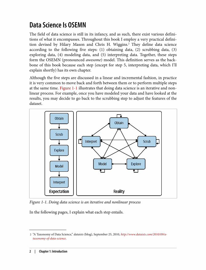
Data Science Is OSEMNThe field of data science is still in its infancy, and as such, there exist various defini‐tions of what it encompasses. Throughout this book I employ a very practical defini‐tion devised by Hilary Mason and Chris H. Wiggins.2 They define data scienceaccording to the following five steps: (1) obtaining data, (2) scrubbing data, (3)exploring data, (4) modeling data, and (5) interpreting data. Together, these stepsform the OSEMN (pronounced awesome) model. This definition serves as the back‐bone of this book because each step (except for step 5, interpreting data, which I’llexplain shortly) has its own chapter.

Although the five steps are discussed in a linear and incremental fashion, in practiceit is very common to move back and forth between them or to perform multiple stepsat the same time. Figure 1-1 illustrates that doing data science is an iterative and non-linear process. For example, once you have modeled your data and have looked at theresults, you may decide to go back to the scrubbing step to adjust the features of thedataset.

Figure 1-1. Doing data science is an iterative and nonlinear process

In the following pages, I explain what each step entails.

2 | Chapter 1: Introduction

Obtaining DataWithout any data, there is little data science you can do. So the first step is obtainingdata. Unless you are fortunate enough to already possess data, you may need to doone or more of the following:

• Download data from another location (e.g., a web page or server)• Query data from a database or API (e.g., MySQL or Twitter)• Extract data from another file (e.g., an HTML file or spreadsheet)• Generate data yourself (e.g., reading sensors or taking surveys)

In Chapter 3, I discuss several methods for obtaining data using the command line.The obtained data will most likely be in plain text, CSV, JSON, HTML, or XML for‐mat. The next step is to scrub this data.

Scrubbing DataIt is not uncommon for the obtained data to have missing values, inconsistencies,errors, weird characters, or uninteresting columns. In such cases, you have to scrub,or clean, the data before you can do anything interesting with it. Common scrubbingoperations include:

• Filtering lines• Extracting certain columns• Replacing values• Extracting words• Handling missing values and duplicates• Converting data from one format to another

While we data scientists love to create exciting data visualizations and insightful mod‐els (steps 3 and 4 of the OSEMN model), usually much effort goes into obtaining andscrubbing the required data first (steps 1 and 2). In Data Jujitsu(O’Reilly), DJ Patilstates that “80% of the work in any data project is in cleaning the data.” In Chapter 5, Idemonstrate how the command line can help accomplish such data scrubbingoperations.

Exploring DataOnce you have scrubbed your data, you are ready to explore it. This is where it getsinteresting, because it’s when you’re exploring that you truly get to know your data. InChapter 7 I show you how the command line can be used to:

Data Science Is OSEMN | 3

• Look at your data• Derive statistics from your data• Create insightful visualizations

Command-line tools used in Chapter 7 include csvstat and rush.

Modeling DataIf you want to explain your data or predict what will happen, you probably want tocreate a statistical model of the data. Techniques to create a model include clustering,classification, regression, and dimensionality reduction. The command line is notsuitable for programming a new type of model from scratch. It is, however, very use‐ful to be able to build a model from the command line. In Chapter 9 I will introduceseveral command-line tools that either build a model locally or employ an API to per‐form the computation in the cloud.

Interpreting DataThe final and perhaps most important step in the OSEMN model is interpreting data.This step involves:

• Drawing conclusions from your data• Evaluating what your results mean• Communicating your results

To be honest, the computer is of little use here, and the command line does not reallycome into play at this stage. Once you have reached this step, it’s up to you. This is theonly step in the OSEMN model that does not have its own chapter. Instead, I referyou to the book Thinking with Data by Max Shron (O’Reilly).

Intermezzo ChaptersBesides the chapters that cover the OSEMN steps, there are four intermezzo chapters.Each discusses a more general topic concerning data science and how the commandline is employed for that. These topics are applicable to any step in the data scienceprocess.

In Chapter 4, I discuss how to create reusable tools for the command line. These per‐sonal tools can come from long commands that you have typed on the command lineor from existing code that you have written in, say, Python or R. Being able to createyour own tools allows you to become more efficient and productive.

4 | Chapter 1: Introduction

Because the command line is an interactive environment for doing data science, itcan become challenging to keep track of your workflow. In Chapter 6, I demonstratea command-line tool called make, which allows you to define your data science work‐flow in terms of tasks and the dependencies between them. This tool increases thereproducibility of your workflow, not only for you but also for your colleagues andpeers.

In Chapter 8, I explain how your commands and tools can be sped up by runningthem in parallel. Using a command-line tool called GNU Parallel, you can applycommand-line tools to very large datasets and run them on multiple cores or even onremote machines.

In Chapter 10, I discuss how to employ the power of the command line in other envi‐ronments and programming languages, such as R, RStudio, Python, Jupyter Note‐books, and even Apache Spark.

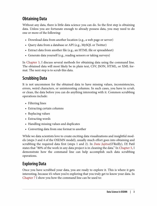
What Is the Command Line?Before I discuss why you should use the command line for data science, let’s take apeek at what the command line actually looks like (it may be already familiar to you).Figures 1-2 and 1-3 show a screenshot of the command line as it appears by defaulton macOS and Ubuntu, respectively. Ubuntu is a particular distribution of GNU/Linux, and it’s the one I’ll be using in this book.

Figure 1-2. Command line on macOS

What Is the Command Line? | 5

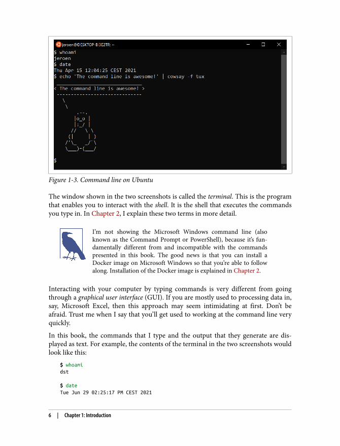
Figure 1-3. Command line on Ubuntu

The window shown in the two screenshots is called the terminal. This is the programthat enables you to interact with the shell. It is the shell that executes the commandsyou type in. In Chapter 2, I explain these two terms in more detail.

I’m not showing the Microsoft Windows command line (alsoknown as the Command Prompt or PowerShell), because it’s fun‐damentally different from and incompatible with the commandspresented in this book. The good news is that you can install aDocker image on Microsoft Windows so that you’re able to followalong. Installation of the Docker image is explained in Chapter 2.

Interacting with your computer by typing commands is very different from goingthrough a graphical user interface (GUI). If you are mostly used to processing data in,say, Microsoft Excel, then this approach may seem intimidating at first. Don’t beafraid. Trust me when I say that you’ll get used to working at the command line veryquickly.

In this book, the commands that I type and the output that they generate are dis‐played as text. For example, the contents of the terminal in the two screenshots wouldlook like this:

$ whoamidst $ dateTue Jun 29 02:25:17 PM CEST 2021

6 | Chapter 1: Introduction

3 Linus Torvalds and Junio C. Hamano, git – the Stupid Content Tracker, version 2.25.1, 2021, https://git-scm.com.

$ echo 'The command line is awesome!' | cowsay -f tux ______________________________< The command line is awesome! > ------------------------------ \ \ .--. |o_o | |:_/ | // \ \ (| | ) /'\_ _/`\ \___)=(___/ $

You’ll notice that each command is preceded by a dollar sign ($). This is called theprompt. The prompt in the two screenshots shows more information, namely theusername, the date, and a penguin. It’s a convention to show only a dollar sign inexamples, because the prompt (1) can change during a session (when you go to a dif‐ferent directory), (2) can be customized by the user (e.g., it can also show the time orthe current git3 branch you’re working on), and (3) is irrelevant for the commandsthemselves.

In the next chapter I’ll explain much more about essential command-line concepts.But first, it’s time to explain why you should learn to use the command line for doingdata science.

Why Data Science at the Command Line?The command line has many great advantages that can really make you a more effi‐cient and productive data scientist. Roughly grouping the advantages, the commandline is agile, augmenting, scalable, extensible, and ubiquitous.

The Command Line Is AgileThe first advantage of the command line is that it allows you to be agile. Data sciencehas a very interactive and exploratory nature, and the environment that you work inneeds to allow for that. The command line achieves this by two means.

First, the command line provides a so-called read-eval-print loop (REPL). This meansthat you type in a command, press Enter, and the command is evaluated immediately.

Why Data Science at the Command Line? | 7

A REPL is often much more convenient for doing data science than the edit-compile-run-debug cycle associated with scripts, large programs, and, say, Hadoop jobs. Yourcommands are executed immediately, may be stopped at will, and can be changedquickly. This short iteration cycle really allows you to play with your data.

Second, the command line is very close to the filesystem. Because data is the mainingredient for doing data science, it is important to be able to work easily with thefiles that contain your dataset. The command line offers many convenient tools forthis.

The Command Line Is AugmentingThe command line integrates well with other technologies. Whatever technologyyour data science workflow currently includes (whether it’s R, Python, or Excel),please know that I’m not suggesting you abandon that workflow. Instead, considerthe command line as an augmenting technology that amplifies the technologiesyou’re currently employing. It can do so in three ways.

First, the command line can act as a glue between many different data science tools.One way to glue tools is by connecting the output from the first tool to the input ofthe second tool. In Chapter 2 I explain how this works.

Second, you can often delegate tasks to the command line from your own environ‐ment. For example, Python, R, and Apache Spark allow you to run command-linetools and capture their output. I demonstrate this with examples in Chapter 10.

Third, you can convert your code (e.g., a Python or R script) into a reusablecommand-line tool. That way, the language that it’s written in doesn’t matter any‐more; it can be used from the command line directly or from any environment thatintegrates with the command line, as mentioned in the previous paragraph. I explainhow to do this in Chapter 4.

In the end, every technology has its strengths and weaknesses, so it’s good to knowseveral technologies and use the one that is most appropriate for the task at hand.Sometimes that means using R, sometimes the command line, and sometimes evenpen and paper. By the end of this book you’ll have a solid understanding of when youshould use the command line, and when you’re better off continuing with your favor‐ite programming language or statistical computing environment.

The Command Line Is ScalableAs I’ve said before, working on the command line is very different from using a GUI.On the command line you do things by typing, whereas with a GUI you do things bypointing and clicking with a mouse.

8 | Chapter 1: Introduction

4 See TOP500, which keeps track of how many supercomputers run Linux.

Everything that you type manually on the command line can also be automatedthrough scripts and tools. This makes it very easy to rerun your commands if youmade a mistake, when the input data has changed, or because your colleague wants toperform the same analysis. Moreover, your commands can be run at specific inter‐vals, on a remote server, and in parallel on many chunks of data (more on that inChapter 8).

Because the command line is automatable, it becomes scalable and repeatable. It’s notstraightforward to automate pointing and clicking, which makes a GUI a less suitableenvironment for doing scalable and repeatable data science.

The Command Line Is ExtensibleThe command line itself was invented over 50 years ago. Its core functionality haslargely remained unchanged, but its tools, which are the workhorses of the commandline, are being developed on a daily basis.

The command line itself is language agnostic. This allows the command-line tools tobe written in many different programming languages. The open source community isproducing many free and high-quality command-line tools that we can use for datascience.

These command-line tools can work together, which makes the command line veryflexible. You can also create your own tools, allowing you to extend the effective func‐tionality of the command line.

The Command Line Is UbiquitousBecause the command line comes with any Unix-like operating system, includingUbuntu Linux and macOS, it can be found in many places. Plus, 100% of the top fivehundred supercomputers are running Linux.4 So if you ever get your hands on one ofthose supercomputers (or if you ever find yourself in Jurassic Park with the doorlocks not working), you’d better know your way around the command line!

But Linux doesn’t run only on supercomputers. It also runs on servers, laptops, andembedded systems. These days, many companies offer cloud computing, where youcan easily launch new machines on the fly. If you ever log in to such a machine (or aserver in general), it’s almost certain that you’ll arrive at the command line.

It’s also important to note that the command line isn’t just hype. This technology hasbeen around for more than five decades, and I’m convinced that it’s here to stay foranother five. Learning how to use the command line (for data science and in general)is therefore a worthwhile investment.

Why Data Science at the Command Line? | 9

SummaryIn this chapter I have introduced you to the OSEMN model for doing data science,which I use as a guide throughout the book. I have provided some background aboutthe Unix command line and hopefully convinced you that it’s a suitable environmentfor doing data science. In the next chapter I’ll show you how to get started by instal‐ling the datasets and tools and explain the fundamental concepts.

For Further Exploration• The book UNIX: A History and a Memoir by Brian W. Kernighan (self-published)

tells the story of Unix, explaining what it is, how it was developed, and why itmatters.

• In 2018, I gave a presentation titled “50 Reasons to Learn the Shell for DoingData Science” at Strata London. You can read the slides if you need even moreconvincing.

• The short but sweet book Thinking with Data by Max Shron (O’Reilly) focuses onthe why instead of the how and provides a framework for defining your data sci‐ence project that will help you ask the right questions and solve the rightproblems.

10 | Chapter 1: Introduction

CHAPTER 2

Getting Started

In this chapter, I’m going to make sure that you have all the prerequisites for doingdata science at the command line. The prerequisites are threefold: (1) having thesame datasets that I use in this book, (2) having a proper environment with all thecommand-line tools that I use throughout this book, and (3) understanding theessential concepts that come into play when using the command line.

First, I describe how to download the datasets. Second, I explain how to install theDocker image, which is a virtual environment based on Ubuntu Linux that containsall the necessary command-line tools. Finally, I go over the essential Unix conceptsthrough examples.

By the end of this chapter, you’ll have everything you need to continue with the firststep of doing data science, namely obtaining data.

Getting the DataThe datasets I use in this book can be obtained as follows:

1. Download the ZIP file from the book’s website.2. Create a new directory. You can give this directory any name you like, but I rec‐

ommend you stick to lowercase letters, numbers, and maybe a hyphen or anunderscore so that the name is easier to work with at the command line—forexample, dsatcl2. Remember where this directory is.

3. Move the ZIP file to that new directory and unpack it.4. This directory now contains one subdirectory per chapter.

11

In the next section I explain how to install the environment containing all thecommand-line tools to work with this data.

Installing the Docker ImageIn this book we use many different command-line tools. Unix often comes with a lotof command-line tools preinstalled and offers many packages that contain more rele‐vant tools. Installing these packages yourself is often not too difficult. However, we’llalso use tools that are not available as packages and require a more manual and moreinvolved installation. So that you can acquire the necessary command-line toolswithout having to go through the installation process for each tool, I encourage you,whether you’re on Windows, macOS, or Linux, to install the Docker image that wascreated specifically for this book.

A Docker image is a bundle of one or more applications together with all their depen‐dencies. A Docker container is an isolated environment that runs an image. You canmanage Docker images and containers using the docker command-line tool (whichis what you’ll do below) or the Docker GUI. In a way, a Docker container is like avirtual machine, only a Docker container uses far fewer resources. At the end of thischapter I suggest some resources for learning more about Docker.

If you still prefer to run the command-line tools natively ratherthan inside a Docker container, then you can, of course, install thecommand-line tools individually yourself. The code to build theDocker image can be found on GitHub and may serve as a guide tohelp you with that. Please be aware that this can be time consumingfor some tools, as they require many nontrivial steps, such ascompiling from source.

To install the Docker image, you first need to download Docker itself from theDocker website. Once it is installed, you invoke the following command on your ter‐minal or command prompt to download the Docker image (don’t type the dollarsign):

$ docker pull datasciencetoolbox/dsatcl2e

You can run the Docker image as follows:

$ docker run --rm -it datasciencetoolbox/dsatcl2e

You’re now inside an isolated environment known as a Docker container that has allthe necessary command-line tools installed. If the following command produces anenthusiastic cow, then you know everything is working correctly:

12 | Chapter 2: Getting Started

$ cowsay "Let's moove\!" ______________< Let's moove! > -------------- \ ^__^ \ (oo)\_______ (__)\ )\/\ ||----w | || ||

If you want to get data in and out of the container, you can add a volume, whichmeans that a local directory gets mapped to a directory inside the container. I recom‐mend that you first create a new directory, navigate to this new directory, and thenrun the following when you’re on macOS or Linux:

$ docker run --rm -it -v "$(pwd)":/data datasciencetoolbox/dsatcl2e

Or run the following when you’re on Windows and using the Command Prompt(also known as cmd):

C:\> docker run --rm -it -v "%cd%":/data datasciencetoolbox/dsatcl2e

Or the following when you’re using Windows PowerShell:

PS C:\> docker run --rm -it -v ${PWD}:/data datasciencetoolbox/dsatcl2e

In the above commands, the option -v instructs docker to map the current directoryto the /data directory inside the container, so this is the place to get data in and out ofthe Docker container.

If you would like to know more about the Docker image, you canvisit it on Docker Hub.

When you’re done, you can shut down the Docker container by typing exit.

Essential Unix ConceptsIn Chapter 1, I briefly showed you what the command line is. Now that you are run‐ning the Docker image, we can really get started. In this section, I discuss several con‐cepts and tools that you will need to know to feel comfortable doing data science atthe command line. If up until now you have been mainly working with graphical userinterfaces, then this might be quite a change. But don’t worry—I’ll start at the begin‐ning and very gradually go on to more advanced topics.

Essential Unix Concepts | 13

1 Richard M. Stallman and David MacKenzie, ls – List Directory Contents, version 8.30, 2019, https://www.gnu.org/software/coreutils.

2 Torbjorn Granlund and Richard M. Stallman, cat – Concatenate Files and Print on the Standard Output, ver‐sion 8.30, 2018, https://www.gnu.org/software/coreutils.

3 Stephen Dolan, jq – Command-Line JSON Processor, version 1.6, 2021, https://stedolan.github.io/jq/4 Ulrich Drepper, seq – Print a Sequence of Numbers, version 8.30, 2019, https://www.gnu.org/software/coreutils.

This section is not a complete course in Unix. I will explain onlythe concepts and tools that are relevant to doing data science. Oneof the advantages of the Docker image is that a lot is already set up.If you wish to know more, consult “For Further Exploration” onpage 33.

The EnvironmentSo you’ve just logged in to a brand-new environment. Before you do anything, it’sworthwhile to get a high-level understanding of this environment, which is roughlydefined by four layers, listed here from the top down:

Command-line toolsFirst and foremost, there are the command-line tools that you work with. We usethem by typing their corresponding commands. There are different types ofcommand-line tools, which I will discuss in the next section. Examples of toolsare ls,1 cat,2 and jq.3

TerminalThe terminal, which is the second layer, is the application that we type our com‐mands in. If you see the following text mentioned in the book:

$ seq 3123

then you would type seq 3 into your terminal and press Enter. (The command-line tool seq,4 as you can see, generates a sequence of numbers.) You do not typethe dollar sign ($). It’s just there to tell you that this is a command you can type inthe terminal. This dollar sign is known as the prompt. The text below seq 3 is theoutput of the command.

ShellThe third layer is the shell. Once we have typed in our command and pressedEnter, the terminal sends that command to the shell. The shell is a program thatinterprets the command. I use the Z shell, but many other shells are available,such as Bash and Fish.

14 | Chapter 2: Getting Started

5 Jim Meyering, pwd – Print Name of Current/Working Directory, version 8.30, 2019, https://www.gnu.org/software/coreutils.

Operating systemThe fourth layer is the operating system, which is GNU/Linux in our case. Linuxis the name of the kernel, which is the heart of the operating system. The kernelis in direct contact with the CPU, disks, and other hardware. The kernel also exe‐cutes our command-line tools. GNU, which stands for “GNU’s not UNIX,” refersto the set of basic tools. The Docker image is based on a particular GNU/Linuxdistribution called Ubuntu.

Executing a Command-Line ToolNow that you have a basic understanding of the environment, it is high time that youtry out some commands. Type the following in your terminal (without the dollarsign) and press Enter:

$ pwd/home/dst

You just executed a command that contained a single command-line tool. The toolpwd5 outputs the name of the directory where you currently are. By default, when youlog in, this is your home directory.

The command-line tool cd, which is a Z shell builtin, allows you to navigate to a dif‐ferent directory:

$ cd /data/ch02 $ pwd /data/ch02 $ cd .. $ pwd /data $ cd ch02

Navigate to the directory /data/ch02.

Print the current directory.

Navigate to the parent directory.

Print the current directory again.

Essential Unix Concepts | 15

6 David MacKenzie and Jim Meyering, head – Output the First Part of Files, version 8.30, 2019, https://www.gnu.org/software/coreutils.

Navigate to the subdirectory ch02.

The part after cd specifies the directory you want to navigate to. Values that comeafter the command are called command-line arguments or options. The two dots referto the parent directory. One dot, by the way, refers to the current directory. Whilecd . wouldn’t have any effect, you’ll still see one dot being used in other places.

Let’s try a different command:

$ head -n 3 movies.txtMatrixStar WarsHome Alone

Here we pass three command-line arguments to head.6 The first one is an option.Here I used the short option -n. Sometimes a short option has a long variant, whichwould be --lines in this case. The second one is a value that belongs to the option.The third one is a filename. This particular command outputs the first three lines ofthe file /data/ch02/movies.txt.

Five Types of Command-Line ToolsI use the term command-line tool a lot, but I haven’t yet explained what I actuallymean by it. I use command-line tool as an umbrella term for anything that can beexecuted from the command line (see Figure 2-1). Under the hood, each command-line tool is one of the following five types:

• A binary executable• A shell builtin• An interpreted script• A shell function• An alias

16 | Chapter 2: Getting Started

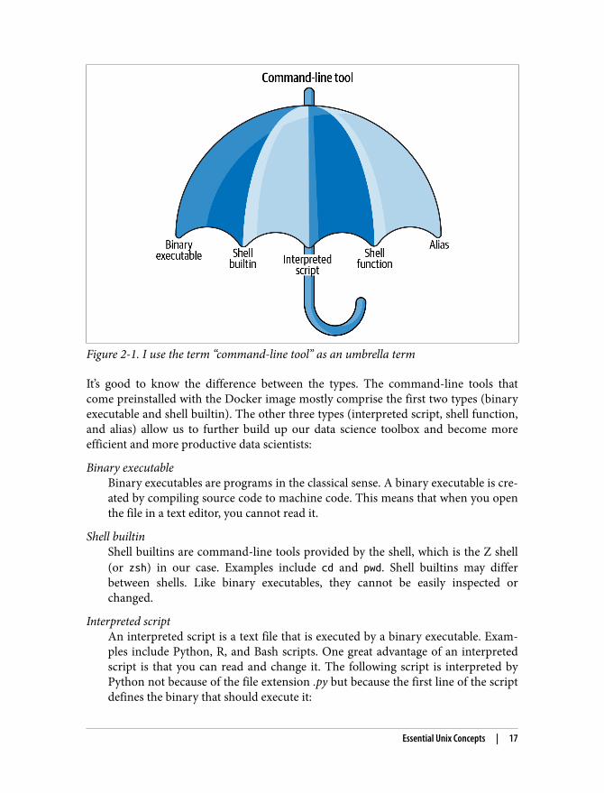
Figure 2-1. I use the term “command-line tool” as an umbrella term

It’s good to know the difference between the types. The command-line tools thatcome preinstalled with the Docker image mostly comprise the first two types (binaryexecutable and shell builtin). The other three types (interpreted script, shell function,and alias) allow us to further build up our data science toolbox and become moreefficient and more productive data scientists:

Binary executableBinary executables are programs in the classical sense. A binary executable is cre‐ated by compiling source code to machine code. This means that when you openthe file in a text editor, you cannot read it.

Shell builtinShell builtins are command-line tools provided by the shell, which is the Z shell(or zsh) in our case. Examples include cd and pwd. Shell builtins may differbetween shells. Like binary executables, they cannot be easily inspected orchanged.

Interpreted scriptAn interpreted script is a text file that is executed by a binary executable. Exam‐ples include Python, R, and Bash scripts. One great advantage of an interpretedscript is that you can read and change it. The following script is interpreted byPython not because of the file extension .py but because the first line of the scriptdefines the binary that should execute it:

Essential Unix Concepts | 17

7 David M. Ihnat and David MacKenzie, paste – Merge Lines of Files, version 8.30, 2019, https://www.gnu.org/software/coreutils.

8 Philip A. Nelson, bc – an Arbitrary Precision Calculator Language, version 1.07.1, 2017, https://www.gnu.org/software/bc.

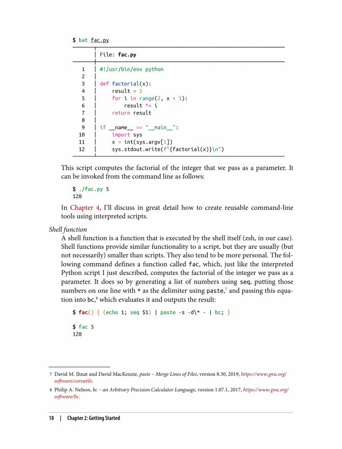
$ bat fac.py───────┬────────────────────────────────────────────────────────────── │ File: fac.py───────┼────────────────────────────────────────────────────────────── 1 │ #!/usr/bin/env python 2 │ 3 │ def factorial(x): 4 │ result = 1 5 │ for i in range(2, x + 1): 6 │ result *= i 7 │ return result 8 │ 9 │ if __name__ == "__main__": 10 │ import sys 11 │ x = int(sys.argv[1]) 12 │ sys.stdout.write(f"{factorial(x)}\n")───────┴──────────────────────────────────────────────────────────────

This script computes the factorial of the integer that we pass as a parameter. Itcan be invoked from the command line as follows:

$ ./fac.py 5120

In Chapter 4, I’ll discuss in great detail how to create reusable command-linetools using interpreted scripts.

Shell functionA shell function is a function that is executed by the shell itself (zsh, in our case).Shell functions provide similar functionality to a script, but they are usually (butnot necessarily) smaller than scripts. They also tend to be more personal. The fol‐lowing command defines a function called fac, which, just like the interpretedPython script I just described, computes the factorial of the integer we pass as aparameter. It does so by generating a list of numbers using seq, putting thosenumbers on one line with * as the delimiter using paste,7 and passing this equa‐tion into bc,8 which evaluates it and outputs the result:

$ fac() { (echo 1; seq $1) | paste -s -d\* - | bc; }

$ fac 5120

18 | Chapter 2: Getting Started

The file ~/.zshrc, which is a configuration file for the Z shell, is a good place todefine your shell functions so that they are always available.

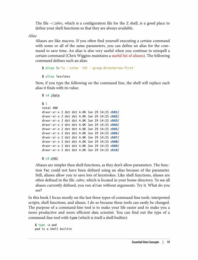
AliasAliases are like macros. If you often find yourself executing a certain commandwith some or all of the same parameters, you can define an alias for the com‐mand to save time. An alias is also very useful when you continue to misspell acertain command (Chris Wiggins maintains a useful list of aliases). The followingcommand defines such an alias:

$ alias l='ls --color -lhF --group-directories-first'

$ alias les=less

Now, if you type the following on the command line, the shell will replace eachalias it finds with its value:

$ cd /data

$ ltotal 40Kdrwxr-xr-x 2 dst dst 4.0K Jun 29 14:25 ch01/drwxr-xr-x 2 dst dst 4.0K Jun 29 14:25 ch02/drwxr-xr-x 2 dst dst 4.0K Jun 29 14:25 ch03/drwxr-xr-x 2 dst dst 4.0K Jun 29 14:25 ch04/drwxr-xr-x 2 dst dst 4.0K Jun 29 14:25 ch05/drwxr-xr-x 2 dst dst 4.0K Jun 29 14:25 ch06/drwxr-xr-x 2 dst dst 4.0K Jun 29 14:25 ch07/drwxr-xr-x 2 dst dst 4.0K Jun 29 14:25 ch08/drwxr-xr-x 2 dst dst 4.0K Jun 29 14:25 ch09/drwxr-xr-x 2 dst dst 4.0K Jun 29 14:25 ch10/

$ cd ch02

Aliases are simpler than shell functions, as they don’t allow parameters. The func‐tion fac could not have been defined using an alias because of the parameter.Still, aliases allow you to save lots of keystrokes. Like shell functions, aliases areoften defined in the file .zshrc, which is located in your home directory. To see allaliases currently defined, you run alias without arguments. Try it. What do yousee?

In this book I focus mostly on the last three types of command-line tools: interpretedscripts, shell functions, and aliases. I do so because these tools can easily be changed.The purpose of a command-line tool is to make your life easier and to make you amore productive and more efficient data scientist. You can find out the type of acommand-line tool with type (which is itself a shell builtin):

$ type -a pwdpwd is a shell builtin

Essential Unix Concepts | 19

9 Eric S. Raymond, The Art of Unix Programming (Addison-Wesley).

10 Jim Meyering, grep – Print Lines That Match Patterns, version 3.4, 2019, https://www.gnu.org/software/grep.11 Paul Rubin and David MacKenzie, wc – Print Newline, Word, and Byte Counts for Each File, version 8.30, 2019,

https://www.gnu.org/software/coreutils.12 Mike Haertel and Paul Eggert, sort – Sort Lines of Text Files, version 8.30, 2019, https://www.gnu.org/software/

coreutils.13 Karel Zak, rev – Reverse Lines Characterwise, version 2.36.1, 2021, https://www.kernel.org/pub/linux/utils/util-

linux.

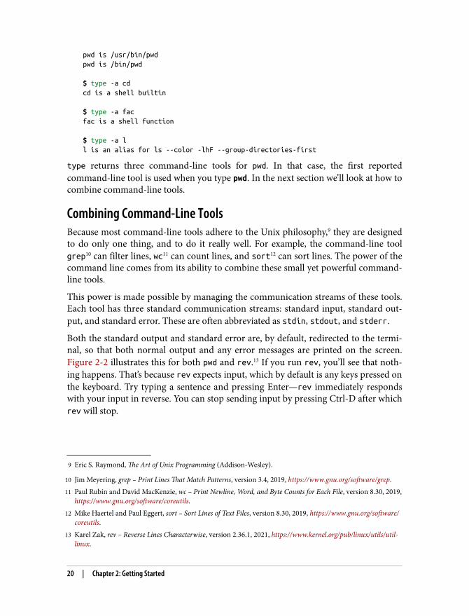
pwd is /usr/bin/pwdpwd is /bin/pwd $ type -a cdcd is a shell builtin $ type -a facfac is a shell function $ type -a ll is an alias for ls --color -lhF --group-directories-first

type returns three command-line tools for pwd. In that case, the first reportedcommand-line tool is used when you type pwd. In the next section we’ll look at how tocombine command-line tools.

Combining Command-Line ToolsBecause most command-line tools adhere to the Unix philosophy,9 they are designedto do only one thing, and to do it really well. For example, the command-line toolgrep10 can filter lines, wc11 can count lines, and sort12 can sort lines. The power of thecommand line comes from its ability to combine these small yet powerful command-line tools.

This power is made possible by managing the communication streams of these tools.Each tool has three standard communication streams: standard input, standard out‐put, and standard error. These are often abbreviated as stdin, stdout, and stderr.

Both the standard output and standard error are, by default, redirected to the termi‐nal, so that both normal output and any error messages are printed on the screen.Figure 2-2 illustrates this for both pwd and rev.13 If you run rev, you’ll see that noth‐ing happens. That’s because rev expects input, which by default is any keys pressed onthe keyboard. Try typing a sentence and pressing Enter—rev immediately respondswith your input in reverse. You can stop sending input by pressing Ctrl-D after whichrev will stop.

20 | Chapter 2: Getting Started

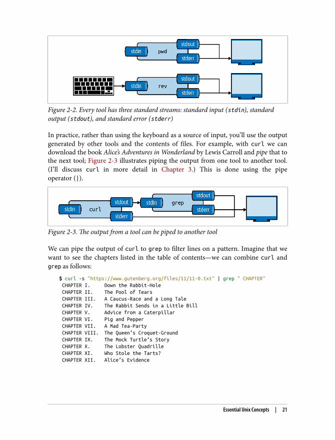
Figure 2-2. Every tool has three standard streams: standard input (stdin), standardoutput (stdout), and standard error (stderr)

In practice, rather than using the keyboard as a source of input, you’ll use the outputgenerated by other tools and the contents of files. For example, with curl we candownload the book Alice’s Adventures in Wonderland by Lewis Carroll and pipe that tothe next tool; Figure 2-3 illustrates piping the output from one tool to another tool.(I’ll discuss curl in more detail in Chapter 3.) This is done using the pipeoperator (|).

Figure 2-3. The output from a tool can be piped to another tool

We can pipe the output of curl to grep to filter lines on a pattern. Imagine that wewant to see the chapters listed in the table of contents—we can combine curl andgrep as follows:

$ curl -s "https://www.gutenberg.org/files/11/11-0.txt" | grep " CHAPTER" CHAPTER I. Down the Rabbit-Hole CHAPTER II. The Pool of Tears CHAPTER III. A Caucus-Race and a Long Tale CHAPTER IV. The Rabbit Sends in a Little Bill CHAPTER V. Advice from a Caterpillar CHAPTER VI. Pig and Pepper CHAPTER VII. A Mad Tea-Party CHAPTER VIII. The Queen’s Croquet-Ground CHAPTER IX. The Mock Turtle’s Story CHAPTER X. The Lobster Quadrille CHAPTER XI. Who Stole the Tarts? CHAPTER XII. Alice’s Evidence

Essential Unix Concepts | 21

And if we want to know how many chapters the book has, we can use wc, which isvery good at counting things:

$ curl -s "https://www.gutenberg.org/files/11/11-0.txt" |> grep " CHAPTER" |> wc -l 12

The option -l specifies that wc should output only the number of lines that arepassed into it. By default, it also returns the number of characters and words.

You can think of piping as an automated copy and paste. Once you get the hang ofcombining tools using the pipe operator, you’ll find that there are virtually no limitsto the combinations you can make.

Redirecting Input and OutputBesides piping the output from one tool to another tool, you can also save it to a file.The file will be saved in the current directory, unless a full path is given. This is calledoutput redirection, and it works as follows:

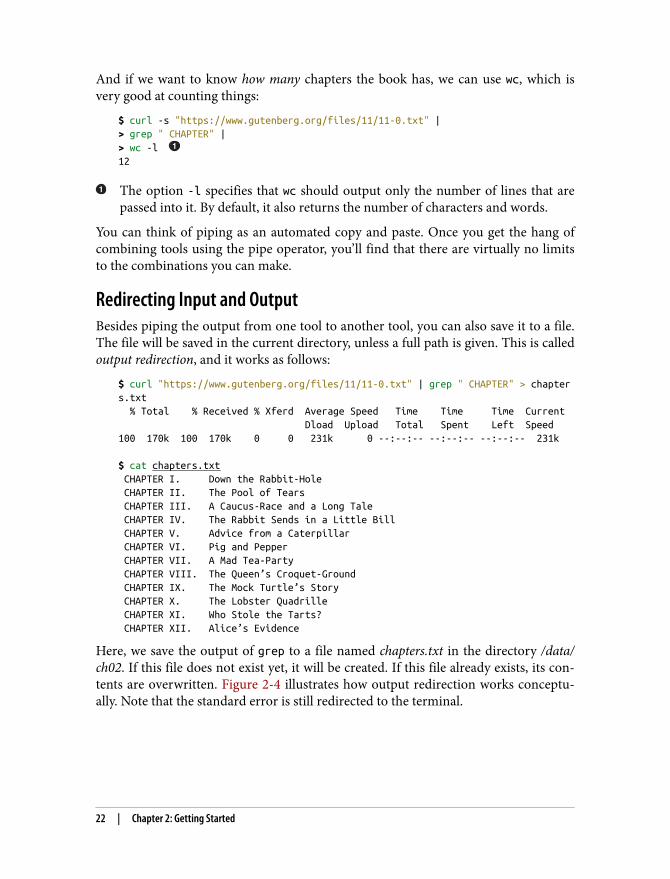
$ curl "https://www.gutenberg.org/files/11/11-0.txt" | grep " CHAPTER" > chapters.txt % Total % Received % Xferd Average Speed Time Time Time Current Dload Upload Total Spent Left Speed100 170k 100 170k 0 0 231k 0 --:--:-- --:--:-- --:--:-- 231k $ cat chapters.txt CHAPTER I. Down the Rabbit-Hole CHAPTER II. The Pool of Tears CHAPTER III. A Caucus-Race and a Long Tale CHAPTER IV. The Rabbit Sends in a Little Bill CHAPTER V. Advice from a Caterpillar CHAPTER VI. Pig and Pepper CHAPTER VII. A Mad Tea-Party CHAPTER VIII. The Queen’s Croquet-Ground CHAPTER IX. The Mock Turtle’s Story CHAPTER X. The Lobster Quadrille CHAPTER XI. Who Stole the Tarts? CHAPTER XII. Alice’s Evidence

Here, we save the output of grep to a file named chapters.txt in the directory /data/ch02. If this file does not exist yet, it will be created. If this file already exists, its con‐tents are overwritten. Figure 2-4 illustrates how output redirection works conceptu‐ally. Note that the standard error is still redirected to the terminal.

22 | Chapter 2: Getting Started

14 Some consider this a “useless use” of cat, arguing that the purpose of cat is to concatenate files, and not usingit for that purpose is a waste of time and costs you a process. I think this is silly. We’ve got more importantthings to do!

Figure 2-4. The output from a tool can be redirected to a file

You can also append the output to a file with >>, meaning the output is added afterthe original contents:

$ echo -n "Hello" > greeting.txt $ echo " World" >> greeting.txt

The tool echo outputs the value you specify. The -n option, which stands for newline,specifies that echo should not output a trailing newline.

Saving the output to a file is useful if you need to store intermediate results, for exam‐ple, to continue with your analysis at a later stage. To use the contents of the file greet‐ing.txt again, we can use cat, which reads a file and prints it:

$ cat greeting.txtHello World $ cat greeting.txt | wc -w 2

The -w option instructs wc to count only words.

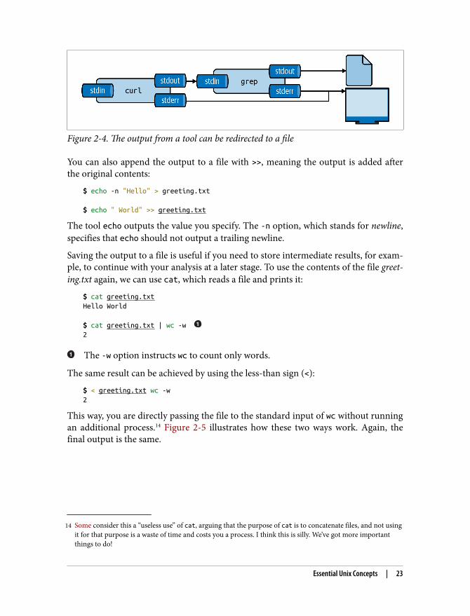
The same result can be achieved by using the less-than sign (<):

$ < greeting.txt wc -w2

This way, you are directly passing the file to the standard input of wc without runningan additional process.14 Figure 2-5 illustrates how these two ways work. Again, thefinal output is the same.

Essential Unix Concepts | 23

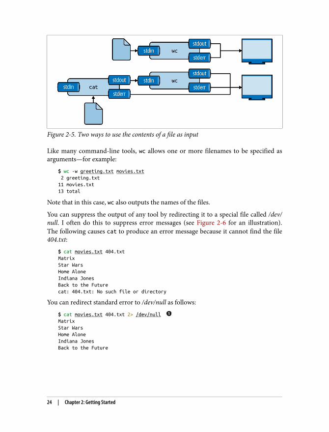
Figure 2-5. Two ways to use the contents of a file as input

Like many command-line tools, wc allows one or more filenames to be specified asarguments—for example:

$ wc -w greeting.txt movies.txt 2 greeting.txt11 movies.txt13 total

Note that in this case, wc also outputs the names of the files.

You can suppress the output of any tool by redirecting it to a special file called /dev/null. I often do this to suppress error messages (see Figure 2-6 for an illustration).The following causes cat to produce an error message because it cannot find the file404.txt:

$ cat movies.txt 404.txtMatrixStar WarsHome AloneIndiana JonesBack to the Futurecat: 404.txt: No such file or directory

You can redirect standard error to /dev/null as follows:

$ cat movies.txt 404.txt 2> /dev/null MatrixStar WarsHome AloneIndiana JonesBack to the Future

24 | Chapter 2: Getting Started

15 Colin Watson and Tollef Fog Heen, sponge – Soak Up Standard Input and Write to a File, version 0.65, 2021,https://joeyh.name/code/moreutils.

16 Jeroen Janssens, dseq – Generate Sequence of Dates, version 0.1, 2021, https://github.com/jeroenjanssens/dsutils.17 Scott Bartram and David MacKenzie, nl – Number Lines of Files, version 8.30, 2020, https://www.gnu.org/soft

ware/coreutils.

The 2 refers to standard error.

Figure 2-6. Redirecting stderr to /dev/null

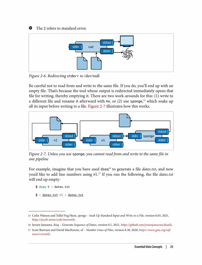
Be careful not to read from and write to the same file. If you do, you’ll end up with anempty file. That’s because the tool whose output is redirected immediately opens thatfile for writing, thereby emptying it. There are two work-arounds for this: (1) write toa different file and rename it afterward with mv, or (2) use sponge,15 which soaks upall its input before writing to a file. Figure 2-7 illustrates how this works.

Figure 2-7. Unless you use sponge, you cannot read from and write to the same file inone pipeline

For example, imagine that you have used dseq16 to generate a file dates.txt, and nowyou’d like to add line numbers using nl.17 If you run the following, the file dates.txtwill end up empty:

$ dseq 5 > dates.txt $ < dates.txt nl > dates.txt

Essential Unix Concepts | 25

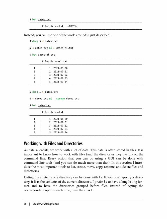
$ bat dates.txt───────┬──────────────────────────────────────────────────────────────────────── │ File: dates.txt <EMPTY>───────┴────────────────────────────────────────────────────────────────────────

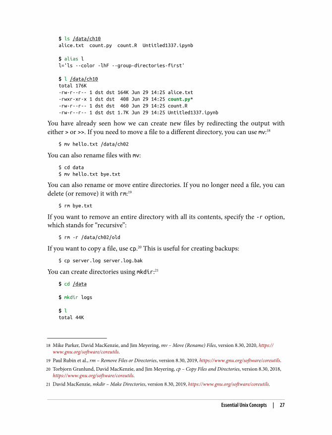
Instead, you can use one of the work-arounds I just described:

$ dseq 5 > dates.txt

$ < dates.txt nl > dates-nl.txt $ bat dates-nl.txt───────┬──────────────────────────────────────────────────────────────────────── │ File: dates-nl.txt───────┼──────────────────────────────────────────────────────────────────────── 1 │ 1 2021-06-30 2 │ 2 2021-07-01 3 │ 3 2021-07-02 4 │ 4 2021-07-03 5 │ 5 2021-07-04───────┴──────────────────────────────────────────────────────────────────────── $ dseq 5 > dates.txt

$ < dates.txt nl | sponge dates.txt $ bat dates.txt───────┬──────────────────────────────────────────────────────────────────────── │ File: dates.txt───────┼──────────────────────────────────────────────────────────────────────── 1 │ 1 2021-06-30 2 │ 2 2021-07-01 3 │ 3 2021-07-02 4 │ 4 2021-07-03 5 │ 5 2021-07-04───────┴────────────────────────────────────────────────────────────────────────

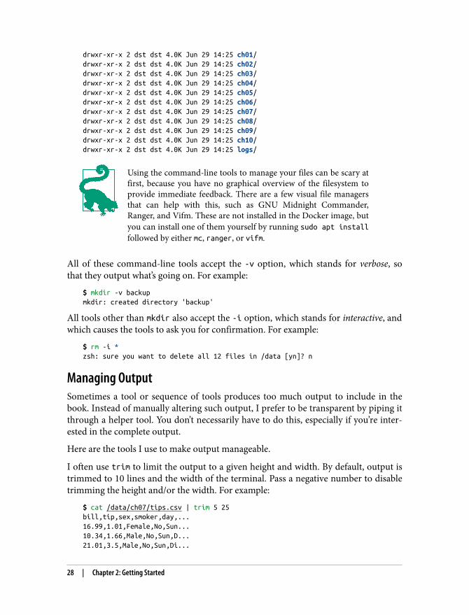
Working with Files and DirectoriesAs data scientists, we work with a lot of data. This data is often stored in files. It isimportant to know how to work with files (and the directories they live in) on thecommand line. Every action that you can do using a GUI can be done withcommand-line tools (and you can do much more than that). In this section I intro‐duce the most important tools to list, create, move, copy, rename, and delete files anddirectories.

Listing the contents of a directory can be done with ls. If you don’t specify a direc‐tory, it lists the contents of the current directory. I prefer ls to have a long listing for‐mat and to have the directories grouped before files. Instead of typing thecorresponding options each time, I use the alias l:

26 | Chapter 2: Getting Started

18 Mike Parker, David MacKenzie, and Jim Meyering, mv – Move (Rename) Files, version 8.30, 2020, https://www.gnu.org/software/coreutils.

19 Paul Rubin et al., rm – Remove Files or Directories, version 8.30, 2019, https://www.gnu.org/software/coreutils.20 Torbjorn Granlund, David MacKenzie, and Jim Meyering, cp – Copy Files and Directories, version 8.30, 2018,

https://www.gnu.org/software/coreutils.21 David MacKenzie, mkdir – Make Directories, version 8.30, 2019, https://www.gnu.org/software/coreutils.

$ ls /data/ch10alice.txt count.py count.R Untitled1337.ipynb $ alias ll='ls --color -lhF --group-directories-first' $ l /data/ch10total 176K-rw-r--r-- 1 dst dst 164K Jun 29 14:25 alice.txt-rwxr-xr-x 1 dst dst 408 Jun 29 14:25 count.py*-rw-r--r-- 1 dst dst 460 Jun 29 14:25 count.R-rw-r--r-- 1 dst dst 1.7K Jun 29 14:25 Untitled1337.ipynb

You have already seen how we can create new files by redirecting the output witheither > or >>. If you need to move a file to a different directory, you can use mv:18

$ mv hello.txt /data/ch02

You can also rename files with mv:

$ cd data$ mv hello.txt bye.txt

You can also rename or move entire directories. If you no longer need a file, you candelete (or remove) it with rm:19

$ rm bye.txt

If you want to remove an entire directory with all its contents, specify the -r option,which stands for “recursive”:

$ rm -r /data/ch02/old

If you want to copy a file, use cp.20 This is useful for creating backups:

$ cp server.log server.log.bak

You can create directories using mkdir:21

$ cd /data $ mkdir logs $ ltotal 44K

Essential Unix Concepts | 27

drwxr-xr-x 2 dst dst 4.0K Jun 29 14:25 ch01/drwxr-xr-x 2 dst dst 4.0K Jun 29 14:25 ch02/drwxr-xr-x 2 dst dst 4.0K Jun 29 14:25 ch03/drwxr-xr-x 2 dst dst 4.0K Jun 29 14:25 ch04/drwxr-xr-x 2 dst dst 4.0K Jun 29 14:25 ch05/drwxr-xr-x 2 dst dst 4.0K Jun 29 14:25 ch06/drwxr-xr-x 2 dst dst 4.0K Jun 29 14:25 ch07/drwxr-xr-x 2 dst dst 4.0K Jun 29 14:25 ch08/drwxr-xr-x 2 dst dst 4.0K Jun 29 14:25 ch09/drwxr-xr-x 2 dst dst 4.0K Jun 29 14:25 ch10/drwxr-xr-x 2 dst dst 4.0K Jun 29 14:25 logs/

Using the command-line tools to manage your files can be scary atfirst, because you have no graphical overview of the filesystem toprovide immediate feedback. There are a few visual file managersthat can help with this, such as GNU Midnight Commander,Ranger, and Vifm. These are not installed in the Docker image, butyou can install one of them yourself by running sudo apt installfollowed by either mc, ranger, or vifm.

All of these command-line tools accept the -v option, which stands for verbose, sothat they output what’s going on. For example:

$ mkdir -v backupmkdir: created directory 'backup'

All tools other than mkdir also accept the -i option, which stands for interactive, andwhich causes the tools to ask you for confirmation. For example:

$ rm -i *zsh: sure you want to delete all 12 files in /data [yn]? n

Managing OutputSometimes a tool or sequence of tools produces too much output to include in thebook. Instead of manually altering such output, I prefer to be transparent by piping itthrough a helper tool. You don’t necessarily have to do this, especially if you’re inter‐ested in the complete output.

Here are the tools I use to make output manageable.

I often use trim to limit the output to a given height and width. By default, output istrimmed to 10 lines and the width of the terminal. Pass a negative number to disabletrimming the height and/or the width. For example:

$ cat /data/ch07/tips.csv | trim 5 25bill,tip,sex,smoker,day,...16.99,1.01,Female,No,Sun...10.34,1.66,Male,No,Sun,D...21.01,3.5,Male,No,Sun,Di...

28 | Chapter 2: Getting Started

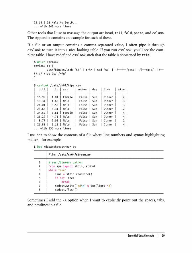
23.68,3.31,Male,No,Sun,D...... with 240 more lines

Other tools that I use to massage the output are head, tail, fold, paste, and column.The Appendix contains an example for each of these.

If a file or an output contains a comma-separated value, I often pipe it throughcsvlook to turn it into a nice-looking table. If you run csvlook, you’ll see the com‐plete table. I have redefined csvlook such that the table is shortened by trim:

$ which csvlookcsvlook () { /usr/bin/csvlook "$@" | trim | sed 's/- | -/──┼──/g;s/| -/├──/g;s/- |/──┤/;s/|/│/g;2s/-/─/g'} $ csvlook /data/ch07/tips.csv│ bill │ tip │ sex │ smoker │ day │ time │ size │├───────┼───────┼────────┼────────┼──────┼────────┼──────┤│ 16.99 │ 1.01 │ Female │ False │ Sun │ Dinner │ 2 ││ 10.34 │ 1.66 │ Male │ False │ Sun │ Dinner │ 3 ││ 21.01 │ 3.50 │ Male │ False │ Sun │ Dinner │ 3 ││ 23.68 │ 3.31 │ Male │ False │ Sun │ Dinner │ 2 ││ 24.59 │ 3.61 │ Female │ False │ Sun │ Dinner │ 4 ││ 25.29 │ 4.71 │ Male │ False │ Sun │ Dinner │ 4 ││ 8.77 │ 2.00 │ Male │ False │ Sun │ Dinner │ 2 ││ 26.88 │ 3.12 │ Male │ False │ Sun │ Dinner │ 4 │... with 236 more lines

I use bat to show the contents of a file where line numbers and syntax highlightingmatter—for example:

$ bat /data/ch04/stream.py───────┬──────────────────────────────────────────────────────────────────────── │ File: /data/ch04/stream.py───────┼──────────────────────────────────────────────────────────────────────── 1 │ #!/usr/bin/env python 2 │ from sys import stdin, stdout 3 │ while True: 4 │ line = stdin.readline() 5 │ if not line: 6 │ break 7 │ stdout.write("%d\n" % int(line)**2) 8 │ stdout.flush()───────┴────────────────────────────────────────────────────────────────────────

Sometimes I add the -A option when I want to explicitly point out the spaces, tabs,and newlines in a file.

Essential Unix Concepts | 29

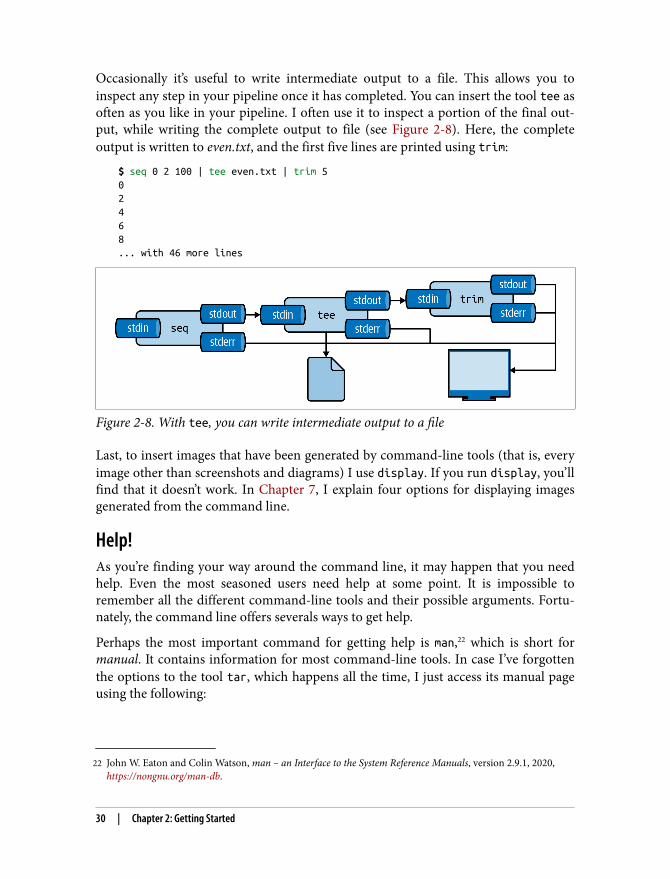
22 John W. Eaton and Colin Watson, man – an Interface to the System Reference Manuals, version 2.9.1, 2020,https://nongnu.org/man-db.

Occasionally it’s useful to write intermediate output to a file. This allows you toinspect any step in your pipeline once it has completed. You can insert the tool tee asoften as you like in your pipeline. I often use it to inspect a portion of the final out‐put, while writing the complete output to file (see Figure 2-8). Here, the completeoutput is written to even.txt, and the first five lines are printed using trim:

$ seq 0 2 100 | tee even.txt | trim 502468... with 46 more lines

Figure 2-8. With tee, you can write intermediate output to a file

Last, to insert images that have been generated by command-line tools (that is, everyimage other than screenshots and diagrams) I use display. If you run display, you’llfind that it doesn’t work. In Chapter 7, I explain four options for displaying imagesgenerated from the command line.

Help!As you’re finding your way around the command line, it may happen that you needhelp. Even the most seasoned users need help at some point. It is impossible toremember all the different command-line tools and their possible arguments. Fortu‐nately, the command line offers severals ways to get help.

Perhaps the most important command for getting help is man,22 which is short formanual. It contains information for most command-line tools. In case I’ve forgottenthe options to the tool tar, which happens all the time, I just access its manual pageusing the following:

30 | Chapter 2: Getting Started

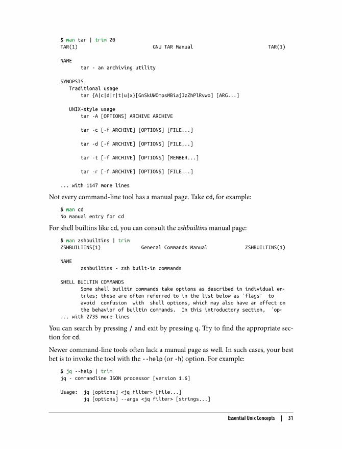
$ man tar | trim 20TAR(1) GNU TAR Manual TAR(1) NAME tar - an archiving utility SYNOPSIS Traditional usage tar {A|c|d|r|t|u|x}[GnSkUWOmpsMBiajJzZhPlRvwo] [ARG...] UNIX-style usage tar -A [OPTIONS] ARCHIVE ARCHIVE tar -c [-f ARCHIVE] [OPTIONS] [FILE...] tar -d [-f ARCHIVE] [OPTIONS] [FILE...] tar -t [-f ARCHIVE] [OPTIONS] [MEMBER...] tar -r [-f ARCHIVE] [OPTIONS] [FILE...] ... with 1147 more lines

Not every command-line tool has a manual page. Take cd, for example:

$ man cdNo manual entry for cd

For shell builtins like cd, you can consult the zshbuiltins manual page:

$ man zshbuiltins | trimZSHBUILTINS(1) General Commands Manual ZSHBUILTINS(1) NAME zshbuiltins - zsh built-in commands SHELL BUILTIN COMMANDS Some shell builtin commands take options as described in individual en‐ tries; these are often referred to in the list below as `flags' to avoid confusion with shell options, which may also have an effect on the behavior of builtin commands. In this introductory section, `op‐... with 2735 more lines

You can search by pressing / and exit by pressing q. Try to find the appropriate sec‐tion for cd.

Newer command-line tools often lack a manual page as well. In such cases, your bestbet is to invoke the tool with the --help (or -h) option. For example:

$ jq --help | trimjq - commandline JSON processor [version 1.6] Usage: jq [options] <jq filter> [file...] jq [options] --args <jq filter> [strings...]

Essential Unix Concepts | 31

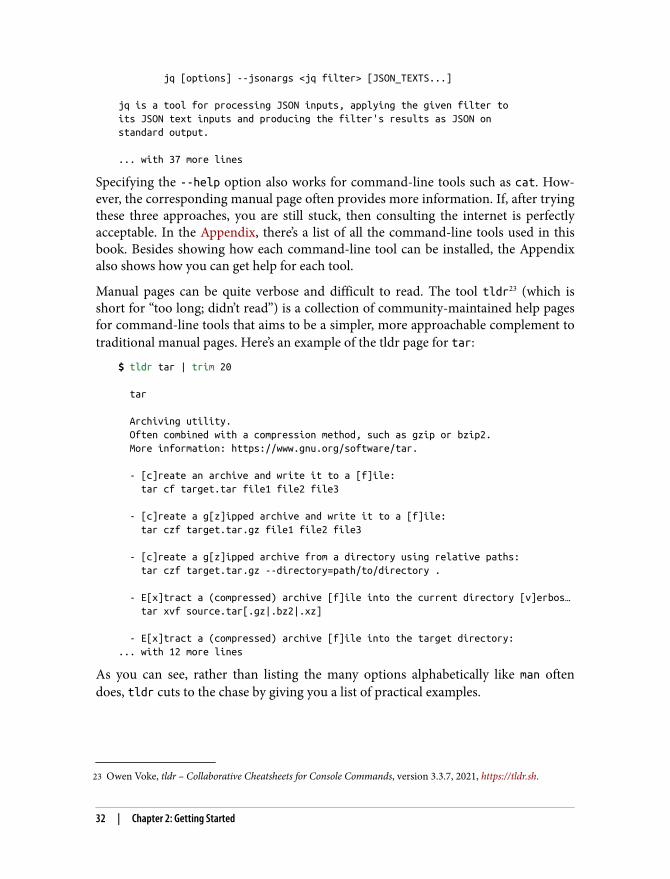
23 Owen Voke, tldr – Collaborative Cheatsheets for Console Commands, version 3.3.7, 2021, https://tldr.sh.

jq [options] --jsonargs <jq filter> [JSON_TEXTS...] jq is a tool for processing JSON inputs, applying the given filter toits JSON text inputs and producing the filter's results as JSON onstandard output. ... with 37 more lines

Specifying the --help option also works for command-line tools such as cat. How‐ever, the corresponding manual page often provides more information. If, after tryingthese three approaches, you are still stuck, then consulting the internet is perfectlyacceptable. In the Appendix, there’s a list of all the command-line tools used in thisbook. Besides showing how each command-line tool can be installed, the Appendixalso shows how you can get help for each tool.

Manual pages can be quite verbose and difficult to read. The tool tldr23 (which isshort for “too long; didn’t read”) is a collection of community-maintained help pagesfor command-line tools that aims to be a simpler, more approachable complement totraditional manual pages. Here’s an example of the tldr page for tar:

$ tldr tar | trim 20 tar Archiving utility. Often combined with a compression method, such as gzip or bzip2. More information: https://www.gnu.org/software/tar. - [c]reate an archive and write it to a [f]ile: tar cf target.tar file1 file2 file3 - [c]reate a g[z]ipped archive and write it to a [f]ile: tar czf target.tar.gz file1 file2 file3 - [c]reate a g[z]ipped archive from a directory using relative paths: tar czf target.tar.gz --directory=path/to/directory . - E[x]tract a (compressed) archive [f]ile into the current directory [v]erbos… tar xvf source.tar[.gz|.bz2|.xz] - E[x]tract a (compressed) archive [f]ile into the target directory:... with 12 more lines

As you can see, rather than listing the many options alphabetically like man oftendoes, tldr cuts to the chase by giving you a list of practical examples.

32 | Chapter 2: Getting Started

SummaryIn this chapter you learned how to get all the required command-line tools by instal‐ling a Docker image. I also went over some essential command-line concepts andhow to get help. Now that you have all the necessary ingredients, you’re ready for thefirst step of the OSEMN model for data science: obtaining data.

For Further Exploration• The subtitle of this book pays homage to the epic Unix Power Tools, 3rd ed. by

Shelley Powers, Jerry Peek, Tim O’Reilly, and Mike Loukides (O’Reilly), andrightly so. With over 51 chapters and more than a thousand pages, Unix PowerTools covers just about everything there is to know about Unix. It weighs morethan four pounds, so you might want to consider getting the ebook.

• The website explainshell parses a command or a sequence of commands and pro‐vides a short explanation of each part. This site is useful for quickly understand‐ing a new command or option without having to skim through the relevantmanual pages.

• Docker is truly a brilliant piece of software. In this chapter I’ve briefly explainedhow to download a Docker image and run a Docker container, but it might beworthwhile to learn how to create your own Docker images. The book Docker:Up & Running, 2nd ed. by Sean P. Kane and Karl Matthias (O’Reilly) is a goodresource as well.

Summary | 33

1 Daniel Stenberg, curl – Transfer a URL, version 7.68.0, 2016, https://curl.haxx.se.2 Christopher Groskopf, in2csv – Convert Common, but Less Awesome, Tabular Data Formats to CSV, version

1.0.5, 2020, https://csvkit.rtfd.org.3 Christopher Groskopf, sql2csv – Execute an SQL Query on a Database and Output the Result to a CSV File,

version 1.0.5, 2020, https://csvkit.rtfd.org.4 John Gilmore and Jay Fenlason, tar – an Archiving Utility, version 1.30, 2014, https://www.gnu.org/software/

tar.

CHAPTER 3

Obtaining Data

This chapter deals with the first step of the OSEMN model: obtaining data. After all,without any data, there is not much data science that we can do. I assume that thedata you need to solve your data science problem already exists. Your first task is toget this data onto your computer (and possibly also inside the Docker container) in aform that you can work with.

According to the Unix philosophy, text is a universal interface. Almost everycommand-line tool takes text as input, produces text as output, or both. This is themain reason why command-line tools can work so well together. However, as we’llsee, even just text can come in multiple forms.

Data can be obtained in several ways—for example, by downloading it from a server,querying a database, or connecting to a Web API. Sometimes the data comes in acompressed form or in a binary format such as a Microsoft Excel Spreadsheet. In thischapter, I discuss several tools that help tackle this from the command line, includingcurl,1 in2csv,2 sql2csv,3 and tar.4

35

OverviewIn this chapter, you’ll learn how to:

• Copy local files to the Docker image• Download data from the internet• Decompress files• Extract data from spreadsheets• Query relational databases• Call web APIs

This chapter starts with the following files:

$ cd /data/ch03 $ ltotal 924K-rw-r--r-- 1 dst dst 627K Jun 29 14:26 logs.tar.gz-rw-r--r-- 1 dst dst 189K Jun 29 14:26 r-datasets.db-rw-r--r-- 1 dst dst 149 Jun 29 14:26 tmnt-basic.csv-rw-r--r-- 1 dst dst 148 Jun 29 14:26 tmnt-missing-newline.csv-rw-r--r-- 1 dst dst 181 Jun 29 14:26 tmnt-with-header.csv-rw-r--r-- 1 dst dst 91K Jun 29 14:26 top2000.xlsx

The instructions for getting these files are in Chapter 2. Any other files are eitherdownloaded or generated using command-line tools.

Copying Local Files to the Docker ContainerA common situation is that you already have the necessary files on your own com‐puter. This section explains how you can get those files into the Docker container.

I mentioned in Chapter 2 that the Docker container is an isolated virtual environ‐ment. Luckily, there is one exception to that: files can be transferred in and out of theDocker container. The local directory from which you ran docker run is mapped to adirectory in the Docker container. This directory is called /data. Note that this is notthe home directory, which is /home/dst.

If you have one or more files on your local computer, and you want to apply somecommand-line tools to them, all you have to do is copy or move the files to that map‐ped directory. Let’s assume that you have a file called logs.csv in your Downloadsdirectory.

If you’re running Windows, open the Command Prompt or PowerShell and run thefollowing two commands:

36 | Chapter 3: Obtaining Data

> cd %UserProfile%\Downloads> copy logs.csv MyDataScienceToolbox\

If you are running Linux or macOS, open a terminal and execute the following com‐mand on your operating system (not inside the Docker container):

$ cp ~/Downloads/logs.csv ~/my-data-science-toolbox

You can also drag and drop the file into the right directory using a graphical file man‐ager such as Windows Explorer or macOS Finder.

Downloading from the InternetThe internet provides, without a doubt, the largest resource for interesting data. Thecommand-line tool curl can be considered the command line’s Swiss Army knifewhen it comes to downloading data from the internet.

Introducing curlWhen you browse a URL, which stands for uniform resource locator, your browserinterprets the data it downloads. For example, the browser renders HTML files, playsvideo files automatically, and shows PDF files. However, when you use curl to accessa URL, it downloads the data and, by default, prints it to standard output. curldoesn’t do any interpretation, but luckily other command-line tools can be used toprocess the data further.

The easiest invocation of curl is to specify a URL as a command-line argument. Let’stry downloading an article from Wikipedia:

$ curl "https://en.wikipedia.org/wiki/List_of_windmills_in_the_Netherlands" |> trim % Total % Received % Xferd Average Speed Time Time Time Current Dload Upload Total Spent Left Speed 0 0 0 0 0 0 0 0 --:--:-- --:--:-- --:--:-- 0<!DOCTYPE html><html class="client-nojs" lang="en" dir="ltr"><head><meta charset="UTF-8"/><title>List of windmills in the Netherlands - Wikipedia</title><script>document.documentElement.className="client-js";RLCONF={"wgBreakFrames":…"wikitext","wgRelevantPageName":"List_of_windmills_in_the_Netherlands","wgRelev…"site.styles":"ready","noscript":"ready","user.styles":"ready","ext.globalCssJs…"ext.growthExperiments.SuggestedEditSession"];</script><script>(RLQ=window.RLQ||[]).push(function(){mw.loader.implement("user.options@…100 244k 100 244k 0 0 1291k 0 --:--:-- --:--:-- --:--:-- 1291k… with 1723 more lines

Remember, trim is used only to make the output fit nicely in the book.

Downloading from the Internet | 37

5 Eric Chiang, pup – Parsing HTML at the Command Line, version 0.4.0, 2016, https://github.com/EricChiang/pup.

As you can see, curl downloads the raw HTML returned by Wikipedia’s server; nointerpretation is being done, and the contents are immediately printed on standardoutput. Because of the URL, you’d think that this article would list all the windmills inthe Netherlands. However, there are apparently so many windmills that each provincehas its own page. Fascinating.

By default, curl outputs a progress meter that shows the download rate and theexpected time of completion. This output isn’t written to standard output but insteadis written to a separate channel known as standard error, so that it doesn’t interferewhen you add another tool to the pipeline. While this information can be usefulwhen downloading very large files, I usually find it distracting, so I specify the -soption to silence this output:

$ curl -s "https://en.wikipedia.org/wiki/List_of_windmills_in_Friesland" |> pup -n 'table.wikitable tr' 234

I’ll discuss pup,5 a handy tool for scraping websites, in more detail in Chapter 5.

And what do you know, there are apparently 234 windmills in the province of Fries‐land alone!

SavingYou can let curl save the output to a file by adding the -O option. The filename willbe based on the last part of the URL:

$ curl -s "https://en.wikipedia.org/wiki/List_of_windmills_in_Friesland" -O $ ltotal 1.4M-rw-r--r-- 1 dst dst 427K Jun 29 14:27 List_of_windmills_in_Friesland-rw-r--r-- 1 dst dst 627K Jun 29 14:26 logs.tar.gz-rw-r--r-- 1 dst dst 189K Jun 29 14:26 r-datasets.db-rw-r--r-- 1 dst dst 149 Jun 29 14:26 tmnt-basic.csv-rw-r--r-- 1 dst dst 148 Jun 29 14:26 tmnt-missing-newline.csv-rw-r--r-- 1 dst dst 181 Jun 29 14:26 tmnt-with-header.csv-rw-r--r-- 1 dst dst 91K Jun 29 14:26 top2000.xlsx

If you don’t like that filename, then you can use the -o option together with a file‐name or redirect the output to a file yourself:

$ curl -s "https://en.wikipedia.org/wiki/List_of_windmills_in_Friesland" > friesland.html

38 | Chapter 3: Obtaining Data

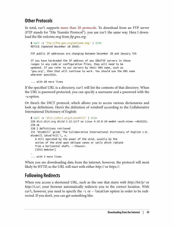
Other ProtocolsIn total, curl supports more than 20 protocols. To download from an FTP server(FTP stands for “File Transfer Protocol”), you use curl the same way. Here I down‐load the file welcome.msg from ftp.gnu.org:

$ curl -s "ftp://ftp.gnu.org/welcome.msg" | trimNOTICE (Updated December 18 2018): FSF public IP addresses are changing between December 20 and January 7th If you have hardcoded the IP address of any GNU/FSF servers in thoseranges in any code or configuration files, they will need to beupdated. If you refer to our servers by their DNS name, such as"gnu.org", then that will continue to work. You should use the DNS namewherever possible. ... with 68 more lines

If the specified URL is a directory, curl will list the contents of that directory. Whenthe URL is password protected, you can specify a username and a password with the-u option.

Or there’s the DICT protocol, which allows you to access various dictionaries andlook up definitions. Here’s the definition of windmill according to the CollaborativeInternational Dictionary of English:

$ curl -s "dict://dict.org/d:windmill" | trim220 dict.dict.org dictd 1.12.1/rf on Linux 4.19.0-10-amd64 <auth.mime> <4623255…250 ok150 1 definitions retrieved151 "Windmill" gcide "The Collaborative International Dictionary of English v.0…Windmill \Wind"mill`\, n. A mill operated by the power of the wind, usually by the action of the wind upon oblique vanes or sails which radiate from a horizontal shaft. --Chaucer. [1913 Webster].... with 2 more lines

When you are downloading data from the internet, however, the protocol will mostlikely be HTTP, so the URL will start with either http:// or https://.

Following RedirectsWhen you access a shortened URL, such as the one that starts with http://bit.ly/ orhttp://t.co/, your browser automatically redirects you to the correct location. Withcurl, however, you need to specify the -L or --location option in order to be redi‐rected. If you don’t, you can get something like:

Downloading from the Internet | 39

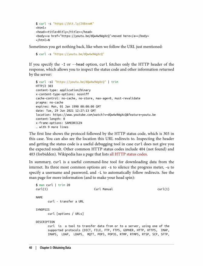
$ curl -s "https://bit.ly/2XBxvwK"<html><head><title>Bitly</title></head><body><a href="https://youtu.be/dQw4w9WgXcQ">moved here</a></body></html>%

Sometimes you get nothing back, like when we follow the URL just mentioned:

$ curl -s "https://youtu.be/dQw4w9WgXcQ"

If you specify the -I or --head option, curl fetches only the HTTP header of theresponse, which allows you to inspect the status code and other information returnedby the server:

$ curl -sI "https://youtu.be/dQw4w9WgXcQ" | trimHTTP/2 303content-type: application/binaryx-content-type-options: nosniffcache-control: no-cache, no-store, max-age=0, must-revalidatepragma: no-cacheexpires: Mon, 01 Jan 1990 00:00:00 GMTdate: Tue, 29 Jun 2021 12:27:13 GMTlocation: https://www.youtube.com/watch?v=dQw4w9WgXcQ&feature=youtu.becontent-length: 0x-frame-options: SAMEORIGIN… with 9 more lines

The first line shows the protocol followed by the HTTP status code, which is 303 inthis case. You can also see the location this URL redirects to. Inspecting the headerand getting the status code is a useful debugging tool in case curl does not give youthe expected result. Other common HTTP status codes include 404 (not found) and403 (forbidden). Wikipedia has a page that lists all HTTP status codes.

In summary, curl is a useful command-line tool for downloading data from theinternet. Its three most common options are -s to silence the progress meter, -u tospecify a username and password, and -L to automatically follow redirects. See theman page for more information (and to make your head spin):

$ man curl | trim 20curl(1) Curl Manual curl(1) NAME curl - transfer a URL SYNOPSIS curl [options / URLs] DESCRIPTION curl is a tool to transfer data from or to a server, using one of the supported protocols (DICT, FILE, FTP, FTPS, GOPHER, HTTP, HTTPS, IMAP, IMAPS, LDAP, LDAPS, MQTT, POP3, POP3S, RTMP, RTMPS, RTSP, SCP, SFTP,

40 | Chapter 3: Obtaining Data

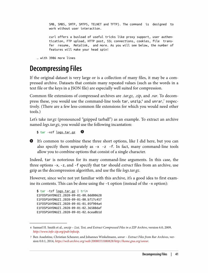
6 Samuel H. Smith et al., unzip – List, Test, and Extract Compressed Files in a ZIP Archive, version 6.0, 2009,http://www.info-zip.org/pub/infozip.

7 Ben Asselstine, Christian Scheurer, and Johannes Winkelmann, unrar – Extract Files from Rar Archives, ver‐sion 0.0.1, 2014, https://web.archive.org/web/20080331080828/http://home.gna.org/unrar.

SMB, SMBS, SMTP, SMTPS, TELNET and TFTP). The command is designed to work without user interaction. curl offers a busload of useful tricks like proxy support, user authen‐ tication, FTP upload, HTTP post, SSL connections, cookies, file trans‐ fer resume, Metalink, and more. As you will see below, the number of features will make your head spin! … with 3986 more lines

Decompressing FilesIf the original dataset is very large or is a collection of many files, it may be a com‐pressed archive. Datasets that contain many repeated values (such as the words in atext file or the keys in a JSON file) are especially well suited for compression.

Common file extensions of compressed archives are .tar.gz, .zip, and .rar. To decom‐press these, you would use the command-line tools tar, unzip,6 and unrar,7 respec‐tively. (There are a few less-common file extensions for which you would need othertools.)

Let’s take tar.gz (pronounced “gzipped tarball”) as an example. To extract an archivenamed logs.tar.gz, you would use the following incantation:

$ tar -xzf logs.tar.gz

It’s common to combine these three short options, like I did here, but you canalso specify them separately as -x -z -f. In fact, many command-line toolsallow you to combine options that consist of a single character.

Indeed, tar is notorious for its many command-line arguments. In this case, thethree options -x, -z, and -f specify that tar should extract files from an archive, usegzip as the decompression algorithm, and use the file logs.tar.gz.

However, since we’re not yet familiar with this archive, it’s a good idea to first exam‐ine its contents. This can be done using the -t option (instead of the -x option):

$ tar -tzf logs.tar.gz | trimE1FOSPSAYDNUZI.2020-09-01-00.0dd00628E1FOSPSAYDNUZI.2020-09-01-00.b717c457E1FOSPSAYDNUZI.2020-09-01-01.05f904a4E1FOSPSAYDNUZI.2020-09-01-02.36588dafE1FOSPSAYDNUZI.2020-09-01-02.6cea8b1d

Decompressing Files | 41

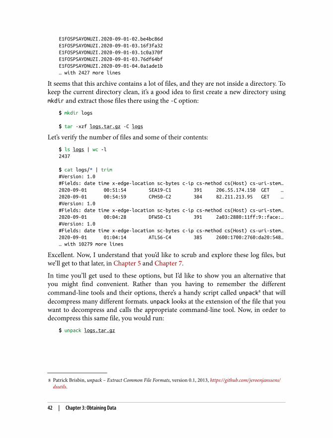
8 Patrick Brisbin, unpack – Extract Common File Formats, version 0.1, 2013, https://github.com/jeroenjanssens/dsutils.

E1FOSPSAYDNUZI.2020-09-01-02.be4bc86dE1FOSPSAYDNUZI.2020-09-01-03.16f3fa32E1FOSPSAYDNUZI.2020-09-01-03.1c0a370fE1FOSPSAYDNUZI.2020-09-01-03.76df64bfE1FOSPSAYDNUZI.2020-09-01-04.0a1ade1b… with 2427 more lines

It seems that this archive contains a lot of files, and they are not inside a directory. Tokeep the current directory clean, it’s a good idea to first create a new directory usingmkdir and extract those files there using the -C option:

$ mkdir logs $ tar -xzf logs.tar.gz -C logs

Let’s verify the number of files and some of their contents:

$ ls logs | wc -l2437 $ cat logs/* | trim#Version: 1.0#Fields: date time x-edge-location sc-bytes c-ip cs-method cs(Host) cs-uri-stem…2020-09-01 00:51:54 SEA19-C1 391 206.55.174.150 GET …2020-09-01 00:54:59 CPH50-C2 384 82.211.213.95 GET …#Version: 1.0#Fields: date time x-edge-location sc-bytes c-ip cs-method cs(Host) cs-uri-stem…2020-09-01 00:04:28 DFW50-C1 391 2a03:2880:11ff:9::face:…#Version: 1.0#Fields: date time x-edge-location sc-bytes c-ip cs-method cs(Host) cs-uri-stem…2020-09-01 01:04:14 ATL56-C4 385 2600:1700:2760:da20:548…… with 10279 more lines

Excellent. Now, I understand that you’d like to scrub and explore these log files, butwe’ll get to that later, in Chapter 5 and Chapter 7.

In time you’ll get used to these options, but I’d like to show you an alternative thatyou might find convenient. Rather than you having to remember the differentcommand-line tools and their options, there’s a handy script called unpack8 that willdecompress many different formats. unpack looks at the extension of the file that youwant to decompress and calls the appropriate command-line tool. Now, in order todecompress this same file, you would run:

$ unpack logs.tar.gz

42 | Chapter 3: Obtaining Data

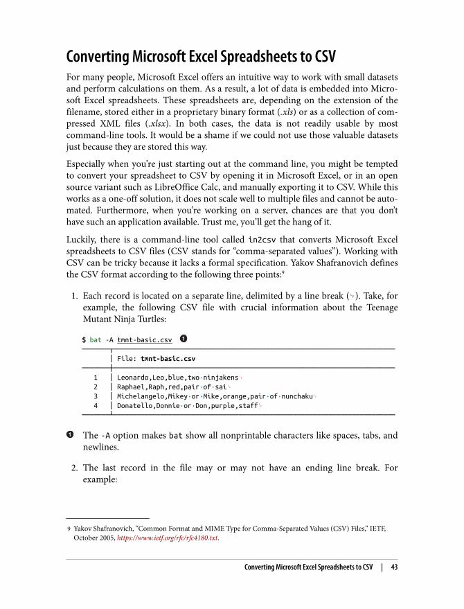
9 Yakov Shafranovich, “Common Format and MIME Type for Comma-Separated Values (CSV) Files,” IETF,October 2005, https://www.ietf.org/rfc/rfc4180.txt.

Converting Microsoft Excel Spreadsheets to CSVFor many people, Microsoft Excel offers an intuitive way to work with small datasetsand perform calculations on them. As a result, a lot of data is embedded into Micro‐soft Excel spreadsheets. These spreadsheets are, depending on the extension of thefilename, stored either in a proprietary binary format (.xls) or as a collection of com‐pressed XML files (.xlsx). In both cases, the data is not readily usable by mostcommand-line tools. It would be a shame if we could not use those valuable datasetsjust because they are stored this way.

Especially when you’re just starting out at the command line, you might be temptedto convert your spreadsheet to CSV by opening it in Microsoft Excel, or in an opensource variant such as LibreOffice Calc, and manually exporting it to CSV. While thisworks as a one-off solution, it does not scale well to multiple files and cannot be auto‐mated. Furthermore, when you’re working on a server, chances are that you don’thave such an application available. Trust me, you’ll get the hang of it.

Luckily, there is a command-line tool called in2csv that converts Microsoft Excelspreadsheets to CSV files (CSV stands for “comma-separated values”). Working withCSV can be tricky because it lacks a formal specification. Yakov Shafranovich definesthe CSV format according to the following three points:9

1. Each record is located on a separate line, delimited by a line break (␊). Take, forexample, the following CSV file with crucial information about the TeenageMutant Ninja Turtles:

$ bat -A tmnt-basic.csv ───────┬──────────────────────────────────────────────────────────────────────── │ File: tmnt-basic.csv───────┼──────────────────────────────────────────────────────────────────────── 1 │ Leonardo,Leo,blue,two·ninjakens␊ 2 │ Raphael,Raph,red,pair·of·sai␊ 3 │ Michelangelo,Mikey·or·Mike,orange,pair·of·nunchaku␊ 4 │ Donatello,Donnie·or·Don,purple,staff␊───────┴────────────────────────────────────────────────────────────────────────

The -A option makes bat show all nonprintable characters like spaces, tabs, andnewlines.

2. The last record in the file may or may not have an ending line break. Forexample:

Converting Microsoft Excel Spreadsheets to CSV | 43

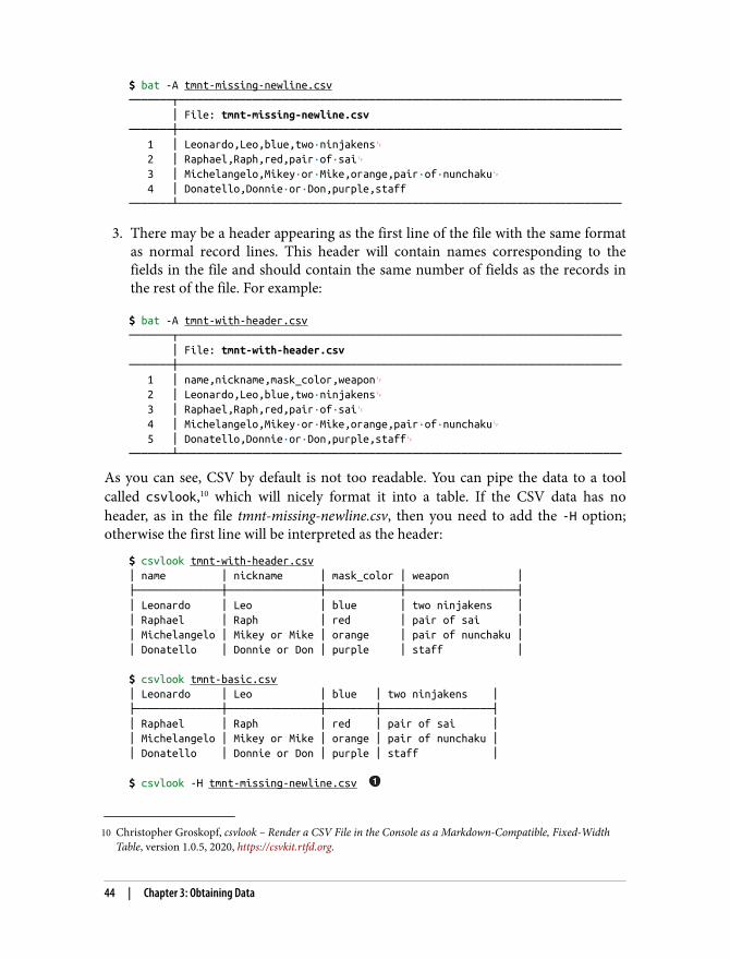
10 Christopher Groskopf, csvlook – Render a CSV File in the Console as a Markdown-Compatible, Fixed-WidthTable, version 1.0.5, 2020, https://csvkit.rtfd.org.

$ bat -A tmnt-missing-newline.csv───────┬──────────────────────────────────────────────────────────────────────── │ File: tmnt-missing-newline.csv───────┼──────────────────────────────────────────────────────────────────────── 1 │ Leonardo,Leo,blue,two·ninjakens␊ 2 │ Raphael,Raph,red,pair·of·sai␊ 3 │ Michelangelo,Mikey·or·Mike,orange,pair·of·nunchaku␊ 4 │ Donatello,Donnie·or·Don,purple,staff───────┴────────────────────────────────────────────────────────────────────────

3. There may be a header appearing as the first line of the file with the same formatas normal record lines. This header will contain names corresponding to thefields in the file and should contain the same number of fields as the records inthe rest of the file. For example:

$ bat -A tmnt-with-header.csv───────┬──────────────────────────────────────────────────────────────────────── │ File: tmnt-with-header.csv───────┼──────────────────────────────────────────────────────────────────────── 1 │ name,nickname,mask_color,weapon␊ 2 │ Leonardo,Leo,blue,two·ninjakens␊ 3 │ Raphael,Raph,red,pair·of·sai␊ 4 │ Michelangelo,Mikey·or·Mike,orange,pair·of·nunchaku␊ 5 │ Donatello,Donnie·or·Don,purple,staff␊───────┴────────────────────────────────────────────────────────────────────────

As you can see, CSV by default is not too readable. You can pipe the data to a toolcalled csvlook,10 which will nicely format it into a table. If the CSV data has noheader, as in the file tmnt-missing-newline.csv, then you need to add the -H option;otherwise the first line will be interpreted as the header:

$ csvlook tmnt-with-header.csv│ name │ nickname │ mask_color │ weapon │├──────────────┼───────────────┼────────────┼──────────────────┤│ Leonardo │ Leo │ blue │ two ninjakens ││ Raphael │ Raph │ red │ pair of sai ││ Michelangelo │ Mikey or Mike │ orange │ pair of nunchaku ││ Donatello │ Donnie or Don │ purple │ staff │ $ csvlook tmnt-basic.csv│ Leonardo │ Leo │ blue │ two ninjakens │├──────────────┼───────────────┼────────┼──────────────────┤│ Raphael │ Raph │ red │ pair of sai ││ Michelangelo │ Mikey or Mike │ orange │ pair of nunchaku ││ Donatello │ Donnie or Don │ purple │ staff │ $ csvlook -H tmnt-missing-newline.csv

44 | Chapter 3: Obtaining Data

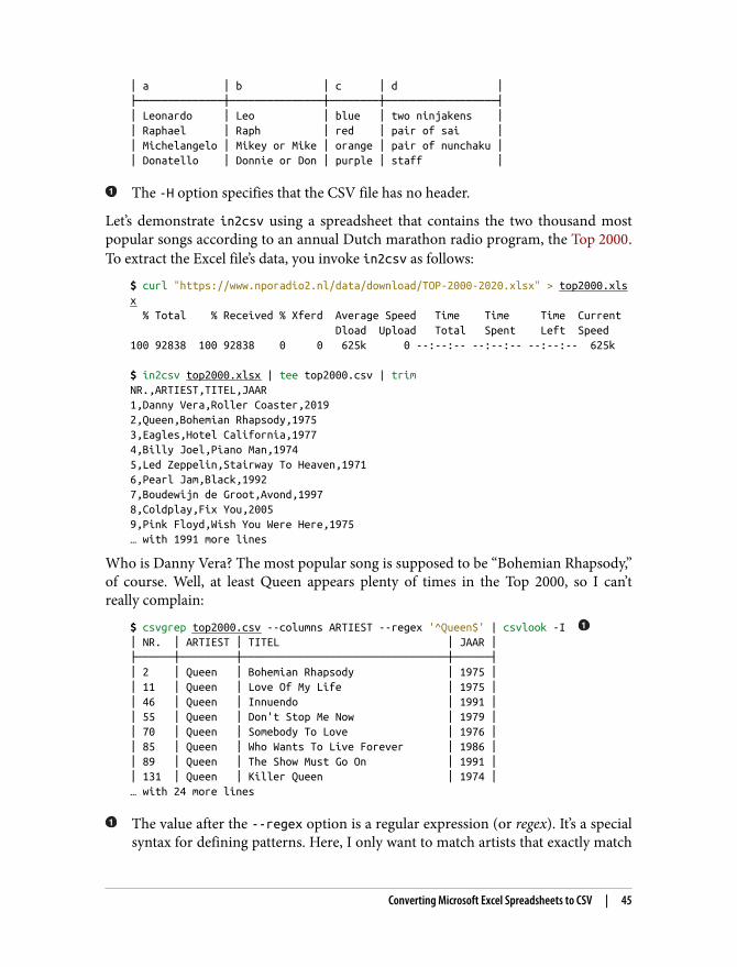
│ a │ b │ c │ d │├──────────────┼───────────────┼────────┼──────────────────┤│ Leonardo │ Leo │ blue │ two ninjakens ││ Raphael │ Raph │ red │ pair of sai ││ Michelangelo │ Mikey or Mike │ orange │ pair of nunchaku ││ Donatello │ Donnie or Don │ purple │ staff │

The -H option specifies that the CSV file has no header.

Let’s demonstrate in2csv using a spreadsheet that contains the two thousand mostpopular songs according to an annual Dutch marathon radio program, the Top 2000.To extract the Excel file’s data, you invoke in2csv as follows:

$ curl "https://www.nporadio2.nl/data/download/TOP-2000-2020.xlsx" > top2000.xlsx % Total % Received % Xferd Average Speed Time Time Time Current Dload Upload Total Spent Left Speed100 92838 100 92838 0 0 625k 0 --:--:-- --:--:-- --:--:-- 625k $ in2csv top2000.xlsx | tee top2000.csv | trimNR.,ARTIEST,TITEL,JAAR1,Danny Vera,Roller Coaster,20192,Queen,Bohemian Rhapsody,19753,Eagles,Hotel California,19774,Billy Joel,Piano Man,19745,Led Zeppelin,Stairway To Heaven,19716,Pearl Jam,Black,19927,Boudewijn de Groot,Avond,19978,Coldplay,Fix You,20059,Pink Floyd,Wish You Were Here,1975… with 1991 more lines

Who is Danny Vera? The most popular song is supposed to be “Bohemian Rhapsody,”of course. Well, at least Queen appears plenty of times in the Top 2000, so I can’treally complain:

$ csvgrep top2000.csv --columns ARTIEST --regex '^Queen$' | csvlook -I │ NR. │ ARTIEST │ TITEL │ JAAR │├──────┼─────────┼─────────────────────────────────┼──────┤│ 2 │ Queen │ Bohemian Rhapsody │ 1975 ││ 11 │ Queen │ Love Of My Life │ 1975 ││ 46 │ Queen │ Innuendo │ 1991 ││ 55 │ Queen │ Don't Stop Me Now │ 1979 ││ 70 │ Queen │ Somebody To Love │ 1976 ││ 85 │ Queen │ Who Wants To Live Forever │ 1986 ││ 89 │ Queen │ The Show Must Go On │ 1991 ││ 131 │ Queen │ Killer Queen │ 1974 │… with 24 more lines

The value after the --regex option is a regular expression (or regex). It’s a specialsyntax for defining patterns. Here, I only want to match artists that exactly match

Converting Microsoft Excel Spreadsheets to CSV | 45

11 Available on GitHub.

“Queen,” so I use the caret (^) and dollar sign ($) to match the start and end ofthe values in the column ARTIEST.

By the way, the tools in2csv, csvgrep, and csvlook are part of csvkit, which is a col‐lection of command-line tools for working with CSV data.

The format of the file is automatically determined by the extension (.xlsx, in thiscase). If you were to pipe the data into in2csv, you would have to specify the formatexplicitly.

A spreadsheet can contain multiple worksheets. in2csv extracts the first worksheetby default. To extract a different worksheet, you need to pass the name of the work‐sheet to the --sheet option. If you’re not sure what the worksheet is called, you canuse the --names option, which prints the names of all the worksheets. Here we seethat top2000.xlsx has only one sheet, named Blad1 (which is Dutch for Sheet1):

$ in2csv --names top2000.xlsxBlad1

Querying Relational DatabasesMany companies store their data in a relational database. Just as with spreadsheets, itwould be great if we could obtain that data from the command line.

Examples of relational databases are MySQL, PostgreSQL, and SQLite. These data‐bases all have a slightly different way of interfacing with them. Some provide acommand-line tool or a command-line interface, while others do not. Moreover, theyare not very consistent when it comes to their usage and output.

Fortunately, there is a command-line tool called sql2csv that is part of the csvkitsuite and that works with many different databases through a common interface,including MySQL, Oracle, PostgreSQL, SQLite, Microsoft SQL Server, and Sybase.The output of sql2csv is, as its name suggests, in CSV format.

We can obtain data from relational databases by executing a SELECT query on them.(sql2csv also support INSERT, UPDATE, and DELETE queries, but that’s not the focus ofthis chapter.)

sql2csv needs two arguments: --db, which specifies the database URL, of which thetypical form is dialect+driver://username:password@host:port/database; and--query, which contains the SELECT query. For example, given an SQLite databasethat contains the standard datasets from R,11 I can select all the rows from the tablemtcars and sort them by the mpg column as follows:

46 | Chapter 3: Obtaining Data

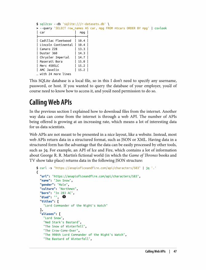
$ sql2csv --db 'sqlite:///r-datasets.db' \> --query 'SELECT row_names AS car, mpg FROM mtcars ORDER BY mpg' | csvlook│ car │ mpg │├─────────────────────┼──────┤│ Cadillac Fleetwood │ 10.4 ││ Lincoln Continental │ 10.4 ││ Camaro Z28 │ 13.3 ││ Duster 360 │ 14.3 ││ Chrysler Imperial │ 14.7 ││ Maserati Bora │ 15.0 ││ Merc 450SLC │ 15.2 ││ AMC Javelin │ 15.2 │… with 24 more lines

This SQLite database is a local file, so in this I don’t need to specify any username,password, or host. If you wanted to query the database of your employer, you’d ofcourse need to know how to access it, and you’d need permission to do so.

Calling Web APIsIn the previous section I explained how to download files from the internet. Anotherway data can come from the internet is through a web API. The number of APIsbeing offered is growing at an increasing rate, which means a lot of interesting datafor us data scientists.

Web APIs are not meant to be presented in a nice layout, like a website. Instead, mostweb APIs return data in a structured format, such as JSON or XML. Having data in astructured form has the advantage that the data can be easily processed by other tools,such as jq. For example, an API of Ice and Fire, which contains a lot of informationabout George R. R. Martin’s fictional world (in which the Game of Thrones books andTV show take place) returns data in the following JSON structure:

$ curl -s "https://anapioficeandfire.com/api/characters/583" | jq '.'{ "url": "https://anapioficeandfire.com/api/characters/583", "name": "Jon Snow", "gender": "Male", "culture": "Northmen", "born": "In 283 AC", "died": "", "titles": [ "Lord Commander of the Night's Watch" ], "aliases": [ "Lord Snow", "Ned Stark's Bastard", "The Snow of Winterfell", "The Crow-Come-Over", "The 998th Lord Commander of the Night's Watch", "The Bastard of Winterfell",

Calling Web APIs | 47

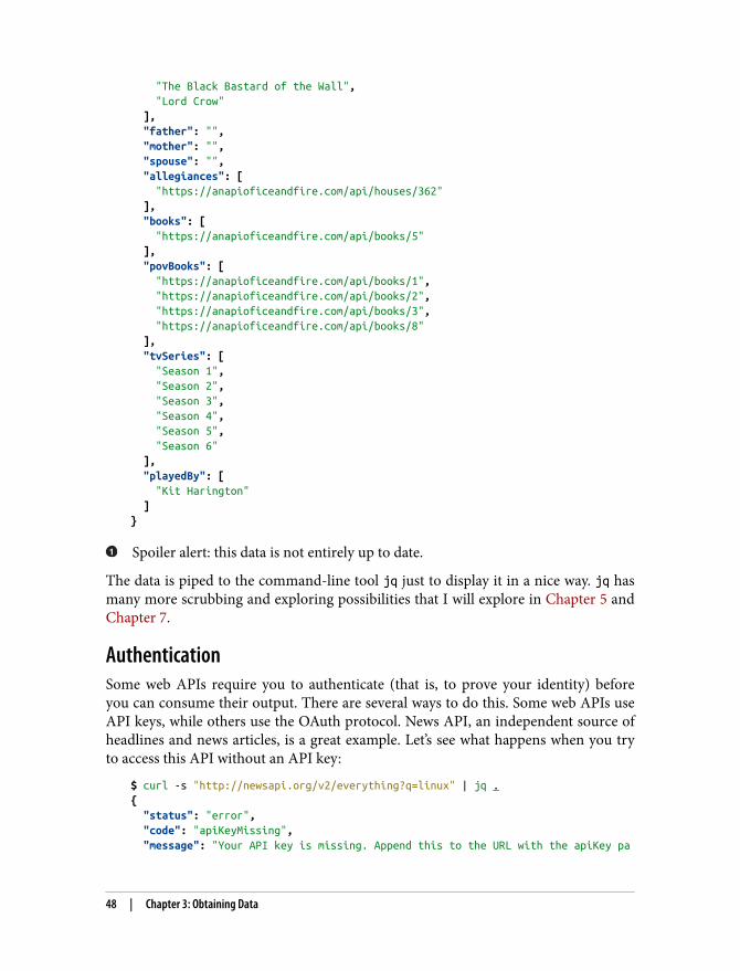
"The Black Bastard of the Wall", "Lord Crow" ], "father": "", "mother": "", "spouse": "", "allegiances": [ "https://anapioficeandfire.com/api/houses/362" ], "books": [ "https://anapioficeandfire.com/api/books/5" ], "povBooks": [ "https://anapioficeandfire.com/api/books/1", "https://anapioficeandfire.com/api/books/2", "https://anapioficeandfire.com/api/books/3", "https://anapioficeandfire.com/api/books/8" ], "tvSeries": [ "Season 1", "Season 2", "Season 3", "Season 4", "Season 5", "Season 6" ], "playedBy": [ "Kit Harington" ]}

Spoiler alert: this data is not entirely up to date.

The data is piped to the command-line tool jq just to display it in a nice way. jq hasmany more scrubbing and exploring possibilities that I will explore in Chapter 5 andChapter 7.

AuthenticationSome web APIs require you to authenticate (that is, to prove your identity) beforeyou can consume their output. There are several ways to do this. Some web APIs useAPI keys, while others use the OAuth protocol. News API, an independent source ofheadlines and news articles, is a great example. Let’s see what happens when you tryto access this API without an API key:

$ curl -s "http://newsapi.org/v2/everything?q=linux" | jq .{ "status": "error", "code": "apiKeyMissing", "message": "Your API key is missing. Append this to the URL with the apiKey pa

48 | Chapter 3: Obtaining Data

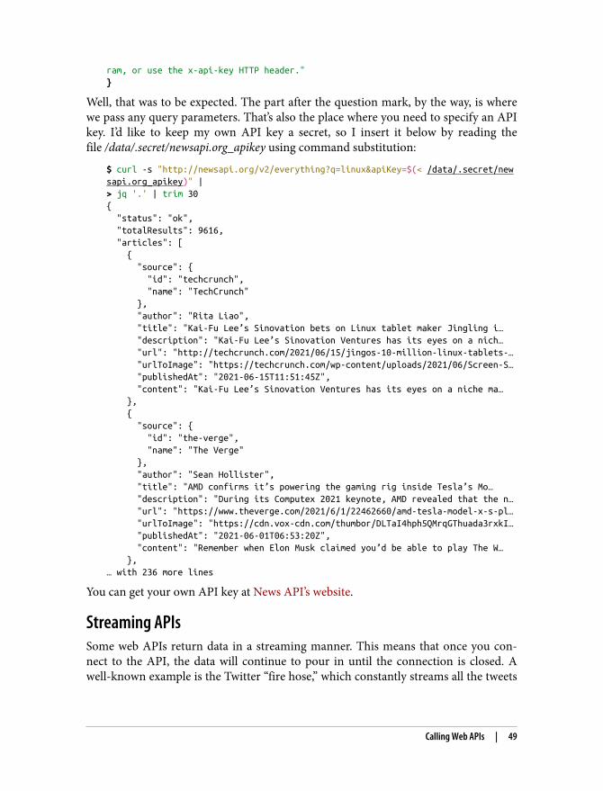
ram, or use the x-api-key HTTP header."}

Well, that was to be expected. The part after the question mark, by the way, is wherewe pass any query parameters. That’s also the place where you need to specify an APIkey. I’d like to keep my own API key a secret, so I insert it below by reading thefile /data/.secret/newsapi.org_apikey using command substitution:

$ curl -s "http://newsapi.org/v2/everything?q=linux&apiKey=$(< /data/.secret/newsapi.org_apikey)" |> jq '.' | trim 30{ "status": "ok", "totalResults": 9616, "articles": [ { "source": { "id": "techcrunch", "name": "TechCrunch" }, "author": "Rita Liao", "title": "Kai-Fu Lee’s Sinovation bets on Linux tablet maker Jingling i… "description": "Kai-Fu Lee’s Sinovation Ventures has its eyes on a nich… "url": "http://techcrunch.com/2021/06/15/jingos-10-million-linux-tablets-… "urlToImage": "https://techcrunch.com/wp-content/uploads/2021/06/Screen-S… "publishedAt": "2021-06-15T11:51:45Z", "content": "Kai-Fu Lee’s Sinovation Ventures has its eyes on a niche ma… }, { "source": { "id": "the-verge", "name": "The Verge" }, "author": "Sean Hollister", "title": "AMD confirms it’s powering the gaming rig inside Tesla’s Mo… "description": "During its Computex 2021 keynote, AMD revealed that the n… "url": "https://www.theverge.com/2021/6/1/22462660/amd-tesla-model-x-s-pl… "urlToImage": "https://cdn.vox-cdn.com/thumbor/DLTaI4hph5QMrqGThuada3rxkI… "publishedAt": "2021-06-01T06:53:20Z", "content": "Remember when Elon Musk claimed you’d be able to play The W… },… with 236 more lines

You can get your own API key at News API’s website.

Streaming APIsSome web APIs return data in a streaming manner. This means that once you con‐nect to the API, the data will continue to pour in until the connection is closed. Awell-known example is the Twitter “fire hose,” which constantly streams all the tweets

Calling Web APIs | 49

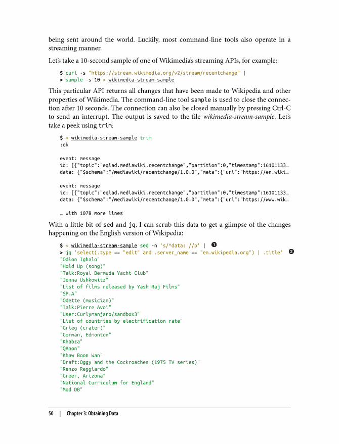
being sent around the world. Luckily, most command-line tools also operate in astreaming manner.

Let’s take a 10-second sample of one of Wikimedia’s streaming APIs, for example:

$ curl -s "https://stream.wikimedia.org/v2/stream/recentchange" |> sample -s 10 > wikimedia-stream-sample

This particular API returns all changes that have been made to Wikipedia and otherproperties of Wikimedia. The command-line tool sample is used to close the connec‐tion after 10 seconds. The connection can also be closed manually by pressing Ctrl-Cto send an interrupt. The output is saved to the file wikimedia-stream-sample. Let’stake a peek using trim:

$ < wikimedia-stream-sample trim:ok event: messageid: [{"topic":"eqiad.mediawiki.recentchange","partition":0,"timestamp":16101133…data: {"$schema":"/mediawiki/recentchange/1.0.0","meta":{"uri":"https://en.wiki… event: messageid: [{"topic":"eqiad.mediawiki.recentchange","partition":0,"timestamp":16101133…data: {"$schema":"/mediawiki/recentchange/1.0.0","meta":{"uri":"https://www.wik… … with 1078 more lines

With a little bit of sed and jq, I can scrub this data to get a glimpse of the changeshappening on the English version of Wikipedia:

$ < wikimedia-stream-sample sed -n 's/^data: //p' | > jq 'select(.type == "edit" and .server_name == "en.wikipedia.org") | .title' "Odion Ighalo""Hold Up (song)""Talk:Royal Bermuda Yacht Club""Jenna Ushkowitz""List of films released by Yash Raj Films""SP.A""Odette (musician)""Talk:Pierre Avoi""User:Curlymanjaro/sandbox3""List of countries by electrification rate""Grieg (crater)""Gorman, Edmonton""Khabza""QAnon""Khaw Boon Wan""Draft:Oggy and the Cockroaches (1975 TV series)""Renzo Reggiardo""Greer, Arizona""National Curriculum for England""Mod DB"

50 | Chapter 3: Obtaining Data

12 Mats Erik Andersson, Andreas Henriksson, and Christoph Biedl, telnet – User Interface to the TELNET Proto‐col, version 0.17, 1999, http://www.hcs.harvard.edu/~dholland/computers/netkit.html.

13 If you cannot connect to the server because someone erased it from the archive memory, then you can alwaysenjoy a recording of the telnet session on YouTube.

"Jordanian Pro League""List of foreign Serie A players"

This sed expression only prints lines that start with data: and prints the partafter the semicolon, which happens to be JSON.

This jq expression prints the title key of JSON objects that have a certain typeand server_name.

Speaking of streaming, did you know that you could stream Star Wars: Episode IV—ANew Hope for free using telnet?12

$ telnet towel.blinkenlights.nl

And after some time, we see that Han Solo did shoot first!

-=== `"', I'll bet you ""o o O O|) have! _\ -/_ _\o/ _ || || |* /|\ / |\ \\ || *** //| | |\\ \\o=*********** // | | | || |\(#'***\\ -==# | | | || |====|* ') '\ |====| /# |/|| | | || | " ( )( ) | || | |-||-| | || | | || | | || | ________________[_][__\________________/__)(_)_____________________

Sure, it’s probably not a good source of data, but there’s nothing wrong with enjoyingan old classic while training your machine learning models.13

SummaryCongratulations, you have finished the first step of the OSEMN model. You’velearned a variety of ways to obtain data, ranging from downloading to querying arelational database. In the next chapter, which is an intermezzo chapter, I’ll teach youhow to create your own command-line tools. But feel free to skip that discussion and

Summary | 51

go on to Chapter 5 (the second step of the OSEMN model) if you cannot wait to learnabout scrubbing data.

For Further Exploration• Looking for a dataset to practice on? The GitHub repository Awesome Public

Datasets lists hundreds of high-quality datasets that are publicly available.• Or perhaps you’d rather practice with an API: the GitHub repository Public APIs

lists many free APIs. City Bikes and The One API are among my favorites.• Writing SQL queries to obtain data from a relational database is an important

skill. The first 15 lessons of the book Sams Teach Yourself SQL in 10 Minutes aDay by Ben Forta (Sams) teach the SELECT statement and its filtering, grouping,and sorting capabilities.

52 | Chapter 3: Obtaining Data

CHAPTER 4

Creating Command-Line Tools

Throughout the book, I’ll introduce you to many commands and combinations ofcommands that basically fit on one line. These are known as one-liners or pipelines.Being able to perform complex tasks with just a one-liner is what makes the com‐mand line powerful. It’s a very different experience from writing and using traditionalprograms.

Some tasks you perform only once, and some you perform more often. Some tasksare very specific, while others can be generalized. If you need to repeat a certain one-liner on a regular basis, it’s worthwhile to turn this into a command-line tool of itsown. So both one-liners and command-line tools have their uses. Recognizing theopportunity to turn a one-liner or existing code into a command-line tool requirespractice and skill. The advantages of a command-line tool are that you don’t have toremember the entire one-liner and that it improves readability if you include it intosome other pipeline. In that sense, you can think of a command-line tool as similar toa function in a programming language.

The benefit of working with a programming language, however, is that the code is inone or more files. This means that you can easily edit and reuse that code. If the codehas parameters, it can even be generalized and reapplied to problems that follow asimilar pattern.

Command-line tools have the best of both worlds: they can be used from the com‐mand line, they accept parameters, and they have to be created only once. In thischapter, you’re going to get familiar with creating command-line tools in two ways.First, I explain how to turn those one-liners into reusable command-line tools. Byadding parameters to your commands, you can add the same flexibility that a pro‐gramming language offers. Subsequently, I demonstrate how to create reusablecommand-line tools from code that’s written in a programming language. By follow‐ing the Unix philosophy, your code can be combined with other command-line tools,

53

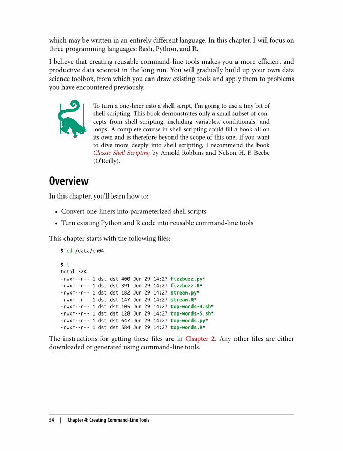
which may be written in an entirely different language. In this chapter, I will focus onthree programming languages: Bash, Python, and R.

I believe that creating reusable command-line tools makes you a more efficient andproductive data scientist in the long run. You will gradually build up your own datascience toolbox, from which you can draw existing tools and apply them to problemsyou have encountered previously.

To turn a one-liner into a shell script, I’m going to use a tiny bit ofshell scripting. This book demonstrates only a small subset of con‐cepts from shell scripting, including variables, conditionals, andloops. A complete course in shell scripting could fill a book all onits own and is therefore beyond the scope of this one. If you wantto dive more deeply into shell scripting, I recommend the bookClassic Shell Scripting by Arnold Robbins and Nelson H. F. Beebe(O’Reilly).

OverviewIn this chapter, you’ll learn how to:

• Convert one-liners into parameterized shell scripts• Turn existing Python and R code into reusable command-line tools

This chapter starts with the following files:

$ cd /data/ch04 $ ltotal 32K-rwxr--r-- 1 dst dst 400 Jun 29 14:27 fizzbuzz.py*-rwxr--r-- 1 dst dst 391 Jun 29 14:27 fizzbuzz.R*-rwxr--r-- 1 dst dst 182 Jun 29 14:27 stream.py*-rwxr--r-- 1 dst dst 147 Jun 29 14:27 stream.R*-rwxr--r-- 1 dst dst 105 Jun 29 14:27 top-words-4.sh*-rwxr--r-- 1 dst dst 128 Jun 29 14:27 top-words-5.sh*-rwxr--r-- 1 dst dst 647 Jun 29 14:27 top-words.py*-rwxr--r-- 1 dst dst 584 Jun 29 14:27 top-words.R*

The instructions for getting these files are in Chapter 2. Any other files are eitherdownloaded or generated using command-line tools.

54 | Chapter 4: Creating Command-Line Tools

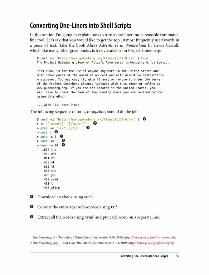
1 Jim Meyering, tr – Translate or Delete Characters, version 8.30, 2018, https://www.gnu.org/software/coreutils.2 Jim Meyering, grep – Print Lines That Match Patterns, version 3.4, 2019, https://www.gnu.org/software/grep.

Converting One-Liners into Shell ScriptsIn this section I’m going to explain how to turn a one-liner into a reusable command-line tool. Let’s say that you would like to get the top 10 most frequently used words ina piece of text. Take the book Alice’s Adventures in Wonderland by Lewis Carroll,which like many other great books, is freely available on Project Gutenberg:

$ curl -sL "https://www.gutenberg.org/files/11/11-0.txt" | trimThe Project Gutenberg eBook of Alice’s Adventures in Wonderland, by Lewis... This eBook is for the use of anyone anywhere in the United States andmost other parts of the world at no cost and with almost no restrictionswhatsoever. You may copy it, give it away or re-use it under the termsof the Project Gutenberg License included with this eBook or online atwww.gutenberg.org. If you are not located in the United States, youwill have to check the laws of the country where you are located beforeusing this eBook. ... with 3751 more lines

The following sequence of tools, or pipeline, should do the job:

$ curl -sL "https://www.gutenberg.org/files/11/11-0.txt" | > tr '[:upper:]' '[:lower:]' | > grep -oE "[a-z\']{2,}" | > sort | > uniq -c | > sort -nr | > head -n 10 1839 the 942 and 811 to 638 of 610 it 553 she 486 you 462 said 435 in 403 alice

Download an ebook using curl.

Convert the entire text to lowercase using tr.1

Extract all the words using grep2 and put each word on a separate line.

Converting One-Liners into Shell Scripts | 55

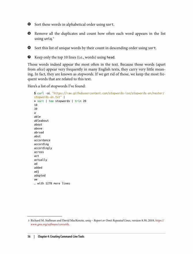
3 Richard M. Stallman and David MacKenzie, uniq – Report or Omit Repeated Lines, version 8.30, 2019, https://www.gnu.org/software/coreutils.

Sort these words in alphabetical order using sort.

Remove all the duplicates and count how often each word appears in the listusing uniq.3

Sort this list of unique words by their count in descending order using sort.

Keep only the top 10 lines (i.e., words) using head.

Those words indeed appear the most often in the text. Because those words (apartfrom alice) appear very frequently in many English texts, they carry very little mean‐ing. In fact, they are known as stopwords. If we get rid of those, we keep the most fre‐quent words that are related to this text.

Here’s a list of stopwords I’ve found:

$ curl -sL "https://raw.githubusercontent.com/stopwords-iso/stopwords-en/master/stopwords-en.txt" |> sort | tee stopwords | trim 201039aableableaboutaboutaboveabroadabstaccordanceaccordingaccordinglyacrossactactuallyadaddedadjadoptedae… with 1278 more lines

56 | Chapter 4: Creating Command-Line Tools

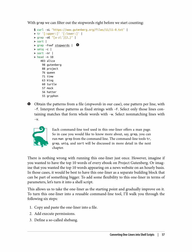
With grep we can filter out the stopwords right before we start counting:

$ curl -sL "https://www.gutenberg.org/files/11/11-0.txt" |> tr '[:upper:]' '[:lower:]' |> grep -oE "[a-z\']{2,}" |> sort |> grep -Fvwf stopwords | > uniq -c |> sort -nr |> head -n 10 403 alice 98 gutenberg 88 project 76 queen 71 time 63 king 60 turtle 57 mock 56 hatter 55 gryphon

Obtain the patterns from a file (stopwords in our case), one pattern per line, with-f. Interpret those patterns as fixed strings with -F. Select only those lines con‐taining matches that form whole words with -w. Select nonmatching lines with-v.

Each command-line tool used in this one-liner offers a man page.So in case you would like to know more about, say, grep, you canrun man grep from the command line. The command-line tools tr,grep, uniq, and sort will be discussed in more detail in the nextchapter.

There is nothing wrong with running this one-liner just once. However, imagine ifyou wanted to have the top 10 words of every ebook on Project Gutenberg. Or imag‐ine that you wanted the top 10 words appearing on a news website on an hourly basis.In those cases, it would be best to have this one-liner as a separate building block thatcan be part of something bigger. To add some flexibility to this one-liner in terms ofparameters, let’s turn it into a shell script.

This allows us to take the one-liner as the starting point and gradually improve on it.To turn this one-liner into a reusable command-line tool, I’ll walk you through thefollowing six steps:

1. Copy and paste the one-liner into a file.2. Add execute permissions.3. Define a so-called shebang.

Converting One-Liners into Shell Scripts | 57

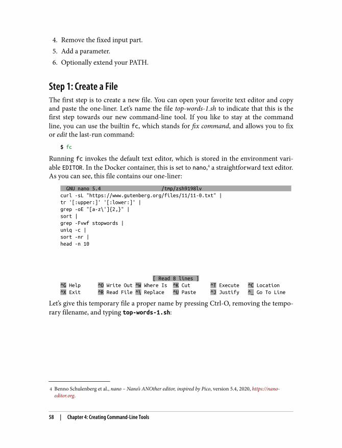
4 Benno Schulenberg et al., nano – Nano’s ANOther editor, inspired by Pico, version 5.4, 2020, https://nano-editor.org.

4. Remove the fixed input part.5. Add a parameter.6. Optionally extend your PATH.

Step 1: Create a FileThe first step is to create a new file. You can open your favorite text editor and copyand paste the one-liner. Let’s name the file top-words-1.sh to indicate that this is thefirst step towards our new command-line tool. If you like to stay at the commandline, you can use the builtin fc, which stands for fix command, and allows you to fixor edit the last-run command:

$ fc

Running fc invokes the default text editor, which is stored in the environment vari‐able EDITOR. In the Docker container, this is set to nano,4 a straightforward text editor.As you can see, this file contains our one-liner:

GNU nano 5.4 /tmp/zsh9198lv curl -sL "https://www.gutenberg.org/files/11/11-0.txt" | tr '[:upper:]' '[:lower:]' | grep -oE "[a-z\']{2,}" | sort | grep -Fvwf stopwords | uniq -c | sort -nr | head -n 10 [ Read 8 lines ] ^G Help ^O Write Out ^W Where Is ^K Cut ^T Execute ^C Location ^X Exit ^R Read File ^\ Replace ^U Paste ^J Justify ^_ Go To Line

Let’s give this temporary file a proper name by pressing Ctrl-O, removing the tempo‐rary filename, and typing top-words-1.sh:

58 | Chapter 4: Creating Command-Line Tools

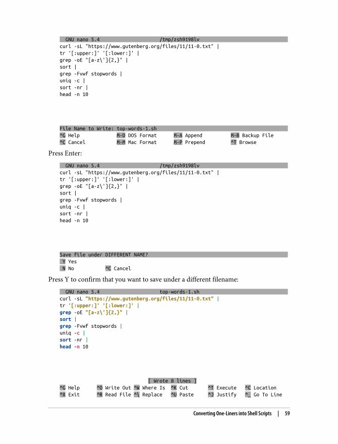
GNU nano 5.4 /tmp/zsh9198lv curl -sL "https://www.gutenberg.org/files/11/11-0.txt" | tr '[:upper:]' '[:lower:]' | grep -oE "[a-z\']{2,}" | sort | grep -Fvwf stopwords | uniq -c | sort -nr | head -n 10 File Name to Write: top-words-1.sh ^G Help M-D DOS Format M-A Append M-B Backup File ^C Cancel M-M Mac Format M-P Prepend ^T Browse

Press Enter:

GNU nano 5.4 /tmp/zsh9198lv curl -sL "https://www.gutenberg.org/files/11/11-0.txt" | tr '[:upper:]' '[:lower:]' | grep -oE "[a-z\']{2,}" | sort | grep -Fvwf stopwords | uniq -c | sort -nr | head -n 10 Save file under DIFFERENT NAME? Y Yes N No ^C Cancel

Press Y to confirm that you want to save under a different filename:

GNU nano 5.4 top-words-1.sh curl -sL "https://www.gutenberg.org/files/11/11-0.txt" | tr '[:upper:]' '[:lower:]' | grep -oE "[a-z\']{2,}" | sort | grep -Fvwf stopwords | uniq -c | sort -nr | head -n 10 [ Wrote 8 lines ] ^G Help ^O Write Out ^W Where Is ^K Cut ^T Execute ^C Location ^X Exit ^R Read File ^\ Replace ^U Paste ^J Justify ^_ Go To Line

Converting One-Liners into Shell Scripts | 59

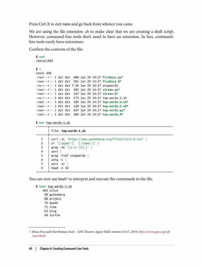
5 Brian Fox and Chet Ramey, bash – GNU Bourne-Again SHell, version 5.0.17, 2019, https://www.gnu.org/software/bash.

Press Ctrl-X to exit nano and go back from whence you came.

We are using the file extension .sh to make clear that we are creating a shell script.However, command-line tools don’t need to have an extension. In fact, command-line tools rarely have extensions.

Confirm the contents of the file:

$ pwd/data/ch04 $ ltotal 44K-rwxr--r-- 1 dst dst 400 Jun 29 14:27 fizzbuzz.py*-rwxr--r-- 1 dst dst 391 Jun 29 14:27 fizzbuzz.R*-rw-r--r-- 1 dst dst 7.5K Jun 29 14:27 stopwords-rwxr--r-- 1 dst dst 182 Jun 29 14:27 stream.py*-rwxr--r-- 1 dst dst 147 Jun 29 14:27 stream.R*-rw-r--r-- 1 dst dst 173 Jun 29 14:27 top-words-1.sh-rwxr--r-- 1 dst dst 105 Jun 29 14:27 top-words-4.sh*-rwxr--r-- 1 dst dst 128 Jun 29 14:27 top-words-5.sh*-rwxr--r-- 1 dst dst 647 Jun 29 14:27 top-words.py*-rwxr--r-- 1 dst dst 584 Jun 29 14:27 top-words.R* $ bat top-words-1.sh───────┬──────────────────────────────────────────────────────────────────────── │ File: top-words-1.sh───────┼──────────────────────────────────────────────────────────────────────── 1 │ curl -sL "https://www.gutenberg.org/files/11/11-0.txt" | 2 │ tr '[:upper:]' '[:lower:]' | 3 │ grep -oE "[a-z\']{2,}" | 4 │ sort | 5 │ grep -Fvwf stopwords | 6 │ uniq -c | 7 │ sort -nr | 8 │ head -n 10───────┴────────────────────────────────────────────────────────────────────────

You can now use bash5 to interpret and execute the commands in the file:

$ bash top-words-1.sh 403 alice 98 gutenberg 88 project 76 queen 71 time 63 king 60 turtle

60 | Chapter 4: Creating Command-Line Tools

6 David MacKenzie and Jim Meyering, chmod – Change File Mode Bits, version 8.30, 2018, https://www.gnu.org/software/coreutils.

57 mock 56 hatter 55 gryphon

This saves you from typing the one-liner again next time.

However, because the file cannot be executed on its own, it’s not yet a real command-line tool. Let’s change that in the next step.

Step 2: Give Permission to ExecuteThe reason we cannot execute our file directly is that we don’t have the correct accesspermissions. In particular, you, as a user, need to have permission to execute the file.In this section we change the access permissions of our file.

In order to compare differences between steps, copy the file to top-words-2.sh usingcp -v top-words-{1,2}.sh.

If you ever want to verify what the brace expansion or any otherform of file expansion leads to, replace the command with echo to just print the result—for example, echo book_{draft,final}.mdor echo agent-{001..007}.

To change the access permissions of a file, we need to use a command-line tool calledchmod,6 which stands for change mode. It changes the file mode bits of a specific file.The following command gives the user (you), permission to execute top-words-2.sh:

$ cp -v top-words-{1,2}.sh'top-words-1.sh' -> 'top-words-2.sh' $ chmod u+x top-words-2.sh

The argument u+x consists of three characters: (1) u indicates that we want to changethe permissions for the user who owns the file, which is you, because you created thefile; (2) + indicates that we want to add a permission; and (3) x indicates the permis‐sions to execute.

Now let’s have a look at the access permissions of both files:

$ l top-words-{1,2}.sh-rw-r--r-- 1 dst dst 173 Jun 29 14:27 top-words-1.sh-rwxr--r-- 1 dst dst 173 Jun 29 14:28 top-words-2.sh*

Converting One-Liners into Shell Scripts | 61

The first column shows the access permissions for each file. For top-words-2.sh, this is-rwxr—r--. The first character, - (hyphen), indicates the file type. A - means regularfile and a d means directory. The next three characters, rwx, indicate the access per‐missions for the user who owns the file. The r and w mean read and write, respec‐tively. (As you can see, top-words-1.sh has a - instead of an x, which means that wecannot execute that file.) The next three characters, rw-, indicate the access permis‐sions for all members of the group that owns the file. Finally, the last three charactersin the column, r--, indicate access permissions for all other users.

Now you can execute the file as follows:

$ ./top-words-2.sh 403 alice 98 gutenberg 88 project 76 queen 71 time 63 king 60 turtle 57 mock 56 hatter 55 gryphon

If you try to execute a file for which you don’t have the correct access permissions, aswith top-words-1.sh, you will see the following error message:

$ ./top-words-1.shzsh: permission denied: ./top-words-1.sh

Step 3: Define a ShebangAlthough we can already execute the file on its own, we should add a so-called she‐bang to the file. The shebang is a special line in the script that instructs the system asto which executable it should use to interpret the commands.

The name shebang comes from the first two characters: a hash (she) and an exclama‐tion mark (bang): #!. It’s not a good idea to leave it out like we have done in the pre‐vious step, because each shell has a different default executable. The Z shell, the onewe’re using throughout the book, uses the executable /bin/sh by default if no shebangis defined. In this case I’d like bash to interpret the commands, as that will give ussome more functionality than sh would.

62 | Chapter 4: Creating Command-Line Tools

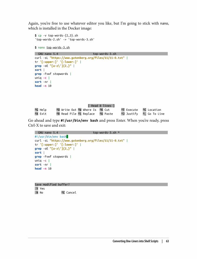
Again, you’re free to use whatever editor you like, but I’m going to stick with nano,which is installed in the Docker image:

$ cp -v top-words-{2,3}.sh'top-words-2.sh' -> 'top-words-3.sh' $ nano top-words-3.sh

GNU nano 5.4 top-words-3.sh curl -sL "https://www.gutenberg.org/files/11/11-0.txt" | tr '[:upper:]' '[:lower:]' | grep -oE "[a-z\']{2,}" | sort | grep -Fvwf stopwords | uniq -c | sort -nr | head -n 10 [ Read 8 lines ] ^G Help ^O Write Out ^W Where Is ^K Cut ^T Execute ^C Location ^X Exit ^R Read File ^\ Replace ^U Paste ^J Justify ^_ Go To Line

Go ahead and type #!/usr/bin/env bash and press Enter. When you’re ready, pressCtrl-X to save and exit:

GNU nano 5.4 top-words-3.sh * #!/usr/bin/env bash curl -sL "https://www.gutenberg.org/files/11/11-0.txt" | tr '[:upper:]' '[:lower:]' | grep -oE "[a-z\']{2,}" | sort | grep -Fvwf stopwords | uniq -c | sort -nr | head -n 10 Save modified buffer? Y Yes N No ^C Cancel

Converting One-Liners into Shell Scripts | 63

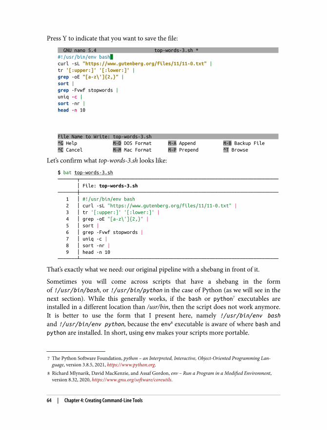
7 The Python Software Foundation, python – an Interpreted, Interactive, Object-Oriented Programming Lan‐guage, version 3.8.5, 2021, https://www.python.org.

8 Richard Mlynarik, David MacKenzie, and Assaf Gordon, env – Run a Program in a Modified Environment,version 8.32, 2020, https://www.gnu.org/software/coreutils.

Press Y to indicate that you want to save the file:

GNU nano 5.4 top-words-3.sh * #!/usr/bin/env bash curl -sL "https://www.gutenberg.org/files/11/11-0.txt" | tr '[:upper:]' '[:lower:]' | grep -oE "[a-z\']{2,}" | sort | grep -Fvwf stopwords | uniq -c | sort -nr | head -n 10 File Name to Write: top-words-3.sh ^G Help M-D DOS Format M-A Append M-B Backup File ^C Cancel M-M Mac Format M-P Prepend ^T Browse

Let’s confirm what top-words-3.sh looks like:

$ bat top-words-3.sh───────┬──────────────────────────────────────────────────────────────────────── │ File: top-words-3.sh───────┼──────────────────────────────────────────────────────────────────────── 1 │ #!/usr/bin/env bash 2 │ curl -sL "https://www.gutenberg.org/files/11/11-0.txt" | 3 │ tr '[:upper:]' '[:lower:]' | 4 │ grep -oE "[a-z\']{2,}" | 5 │ sort | 6 │ grep -Fvwf stopwords | 7 │ uniq -c | 8 │ sort -nr | 9 │ head -n 10───────┴────────────────────────────────────────────────────────────────────────

That’s exactly what we need: our original pipeline with a shebang in front of it.

Sometimes you will come across scripts that have a shebang in the formof !/usr/bin/bash, or !/usr/bin/python in the case of Python (as we will see in thenext section). While this generally works, if the bash or python7 executables areinstalled in a different location than /usr/bin, then the script does not work anymore.It is better to use the form that I present here, namely !/usr/bin/env bash

and !/usr/bin/env python, because the env8 executable is aware of where bash andpython are installed. In short, using env makes your scripts more portable.

64 | Chapter 4: Creating Command-Line Tools

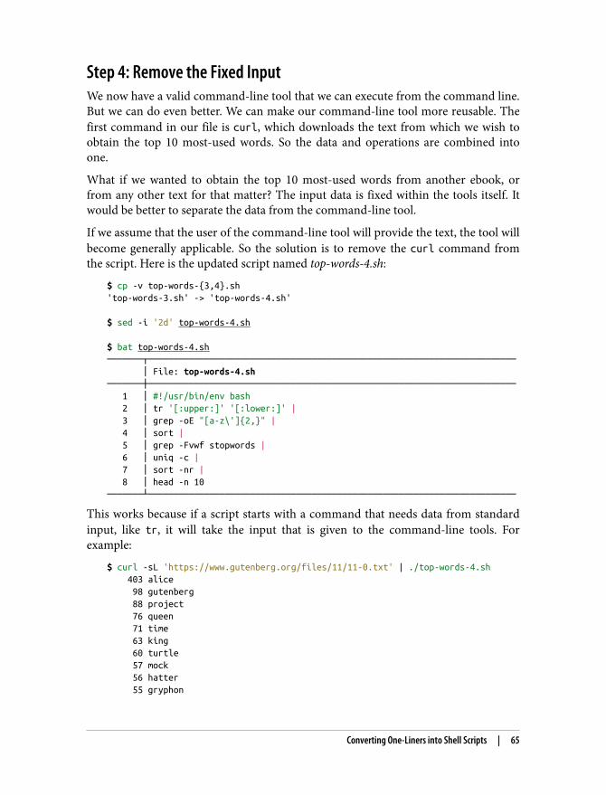
Step 4: Remove the Fixed InputWe now have a valid command-line tool that we can execute from the command line.But we can do even better. We can make our command-line tool more reusable. Thefirst command in our file is curl, which downloads the text from which we wish toobtain the top 10 most-used words. So the data and operations are combined intoone.

What if we wanted to obtain the top 10 most-used words from another ebook, orfrom any other text for that matter? The input data is fixed within the tools itself. Itwould be better to separate the data from the command-line tool.

If we assume that the user of the command-line tool will provide the text, the tool willbecome generally applicable. So the solution is to remove the curl command fromthe script. Here is the updated script named top-words-4.sh:

$ cp -v top-words-{3,4}.sh'top-words-3.sh' -> 'top-words-4.sh' $ sed -i '2d' top-words-4.sh $ bat top-words-4.sh───────┬──────────────────────────────────────────────────────────────────────── │ File: top-words-4.sh───────┼──────────────────────────────────────────────────────────────────────── 1 │ #!/usr/bin/env bash 2 │ tr '[:upper:]' '[:lower:]' | 3 │ grep -oE "[a-z\']{2,}" | 4 │ sort | 5 │ grep -Fvwf stopwords | 6 │ uniq -c | 7 │ sort -nr | 8 │ head -n 10───────┴────────────────────────────────────────────────────────────────────────

This works because if a script starts with a command that needs data from standardinput, like tr, it will take the input that is given to the command-line tools. Forexample:

$ curl -sL 'https://www.gutenberg.org/files/11/11-0.txt' | ./top-words-4.sh 403 alice 98 gutenberg 88 project 76 queen 71 time 63 king 60 turtle 57 mock 56 hatter 55 gryphon

Converting One-Liners into Shell Scripts | 65

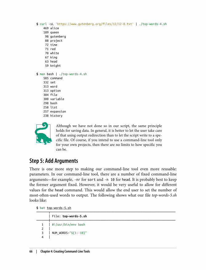
$ curl -sL 'https://www.gutenberg.org/files/12/12-0.txt' | ./top-words-4.sh 469 alice 189 queen 98 gutenberg 88 project 72 time 71 red 70 white 67 king 63 head 59 knight $ man bash | ./top-words-4.sh 585 command 332 set 313 word 313 option 304 file 300 variable 298 bash 258 list 257 expansion 238 history

Although we have not done so in our script, the same principleholds for saving data. In general, it is better to let the user take careof that using output redirection than to let the script write to a spe‐cific file. Of course, if you intend to use a command-line tool onlyfor your own projects, then there are no limits to how specific youcan be.

Step 5: Add ArgumentsThere is one more step to making our command-line tool even more reusable:parameters. In our command-line tool, there are a number of fixed command-linearguments—for example, -nr for sort and -n 10 for head. It is probably best to keepthe former argument fixed. However, it would be very useful to allow for differentvalues for the head command. This would allow the end user to set the number ofmost-often-used words to output. The following shows what our file top-words-5.shlooks like:

$ bat top-words-5.sh───────┬──────────────────────────────────────────────────────────────────────── │ File: top-words-5.sh───────┼──────────────────────────────────────────────────────────────────────── 1 │ #!/usr/bin/env bash 2 │ 3 │ NUM_WORDS="${1:-10}" 4 │

66 | Chapter 4: Creating Command-Line Tools

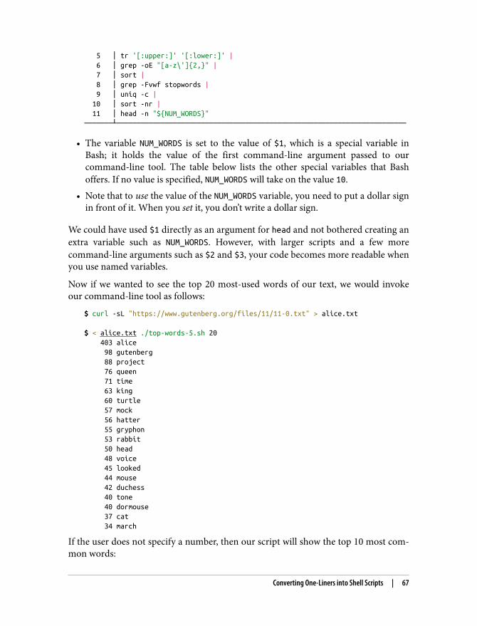
5 │ tr '[:upper:]' '[:lower:]' | 6 │ grep -oE "[a-z\']{2,}" | 7 │ sort | 8 │ grep -Fvwf stopwords | 9 │ uniq -c | 10 │ sort -nr | 11 │ head -n "${NUM_WORDS}"───────┴────────────────────────────────────────────────────────────────────────

• The variable NUM_WORDS is set to the value of $1, which is a special variable inBash; it holds the value of the first command-line argument passed to ourcommand-line tool. The table below lists the other special variables that Bashoffers. If no value is specified, NUM_WORDS will take on the value 10.

• Note that to use the value of the NUM_WORDS variable, you need to put a dollar signin front of it. When you set it, you don’t write a dollar sign.

We could have used $1 directly as an argument for head and not bothered creating anextra variable such as NUM_WORDS. However, with larger scripts and a few morecommand-line arguments such as $2 and $3, your code becomes more readable whenyou use named variables.

Now if we wanted to see the top 20 most-used words of our text, we would invokeour command-line tool as follows:

$ curl -sL "https://www.gutenberg.org/files/11/11-0.txt" > alice.txt $ < alice.txt ./top-words-5.sh 20 403 alice 98 gutenberg 88 project 76 queen 71 time 63 king 60 turtle 57 mock 56 hatter 55 gryphon 53 rabbit 50 head 48 voice 45 looked 44 mouse 42 duchess 40 tone 40 dormouse 37 cat 34 march

If the user does not specify a number, then our script will show the top 10 most com‐mon words:

Converting One-Liners into Shell Scripts | 67

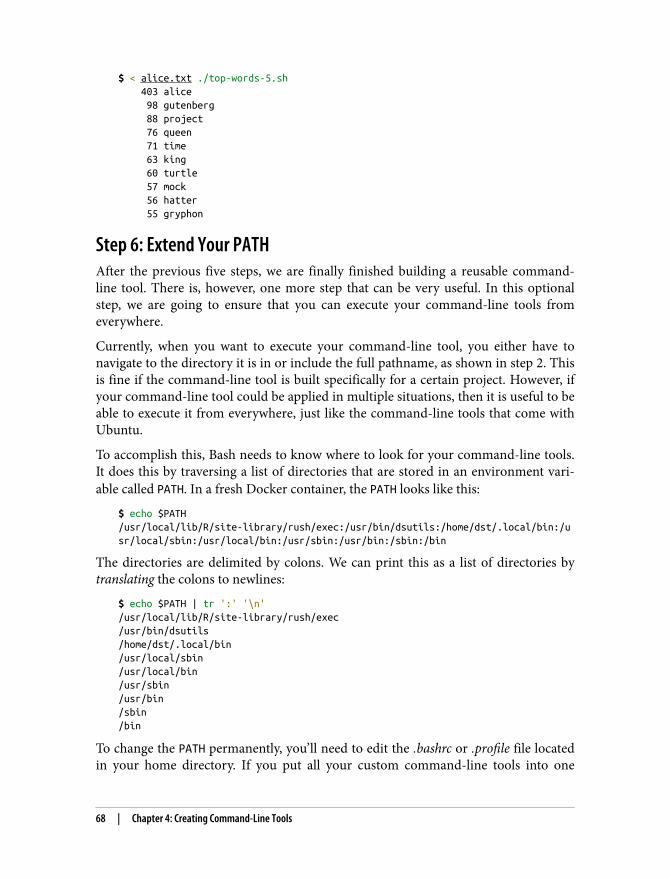
$ < alice.txt ./top-words-5.sh 403 alice 98 gutenberg 88 project 76 queen 71 time 63 king 60 turtle 57 mock 56 hatter 55 gryphon

Step 6: Extend Your PATHAfter the previous five steps, we are finally finished building a reusable command-line tool. There is, however, one more step that can be very useful. In this optionalstep, we are going to ensure that you can execute your command-line tools fromeverywhere.

Currently, when you want to execute your command-line tool, you either have tonavigate to the directory it is in or include the full pathname, as shown in step 2. Thisis fine if the command-line tool is built specifically for a certain project. However, ifyour command-line tool could be applied in multiple situations, then it is useful to beable to execute it from everywhere, just like the command-line tools that come withUbuntu.

To accomplish this, Bash needs to know where to look for your command-line tools.It does this by traversing a list of directories that are stored in an environment vari‐able called PATH. In a fresh Docker container, the PATH looks like this:

$ echo $PATH/usr/local/lib/R/site-library/rush/exec:/usr/bin/dsutils:/home/dst/.local/bin:/usr/local/sbin:/usr/local/bin:/usr/sbin:/usr/bin:/sbin:/bin

The directories are delimited by colons. We can print this as a list of directories bytranslating the colons to newlines:

$ echo $PATH | tr ':' '\n'/usr/local/lib/R/site-library/rush/exec/usr/bin/dsutils/home/dst/.local/bin/usr/local/sbin/usr/local/bin/usr/sbin/usr/bin/sbin/bin

To change the PATH permanently, you’ll need to edit the .bashrc or .profile file locatedin your home directory. If you put all your custom command-line tools into one

68 | Chapter 4: Creating Command-Line Tools

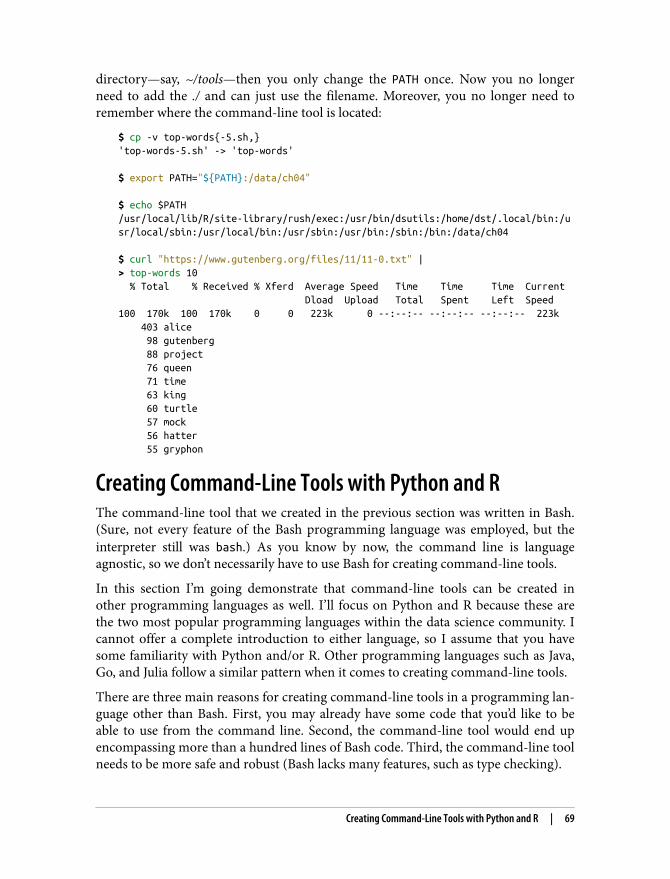
directory—say, ~/tools—then you only change the PATH once. Now you no longerneed to add the ./ and can just use the filename. Moreover, you no longer need toremember where the command-line tool is located:

$ cp -v top-words{-5.sh,}'top-words-5.sh' -> 'top-words' $ export PATH="${PATH}:/data/ch04" $ echo $PATH/usr/local/lib/R/site-library/rush/exec:/usr/bin/dsutils:/home/dst/.local/bin:/usr/local/sbin:/usr/local/bin:/usr/sbin:/usr/bin:/sbin:/bin:/data/ch04 $ curl "https://www.gutenberg.org/files/11/11-0.txt" |> top-words 10 % Total % Received % Xferd Average Speed Time Time Time Current Dload Upload Total Spent Left Speed100 170k 100 170k 0 0 223k 0 --:--:-- --:--:-- --:--:-- 223k 403 alice 98 gutenberg 88 project 76 queen 71 time 63 king 60 turtle 57 mock 56 hatter 55 gryphon

Creating Command-Line Tools with Python and RThe command-line tool that we created in the previous section was written in Bash.(Sure, not every feature of the Bash programming language was employed, but theinterpreter still was bash.) As you know by now, the command line is languageagnostic, so we don’t necessarily have to use Bash for creating command-line tools.

In this section I’m going demonstrate that command-line tools can be created inother programming languages as well. I’ll focus on Python and R because these arethe two most popular programming languages within the data science community. Icannot offer a complete introduction to either language, so I assume that you havesome familiarity with Python and/or R. Other programming languages such as Java,Go, and Julia follow a similar pattern when it comes to creating command-line tools.

There are three main reasons for creating command-line tools in a programming lan‐guage other than Bash. First, you may already have some code that you’d like to beable to use from the command line. Second, the command-line tool would end upencompassing more than a hundred lines of Bash code. Third, the command-line toolneeds to be more safe and robust (Bash lacks many features, such as type checking).

Creating Command-Line Tools with Python and R | 69

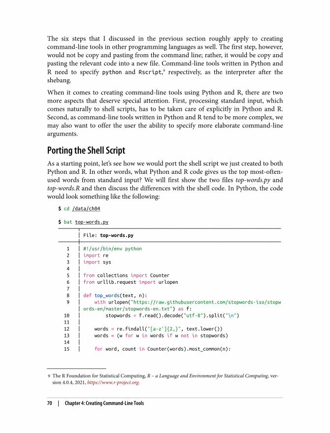
9 The R Foundation for Statistical Computing, R – a Language and Environment for Statistical Computing, ver‐sion 4.0.4, 2021, https://www.r-project.org.

The six steps that I discussed in the previous section roughly apply to creatingcommand-line tools in other programming languages as well. The first step, however,would not be copy and pasting from the command line; rather, it would be copy andpasting the relevant code into a new file. Command-line tools written in Python andR need to specify python and Rscript,9 respectively, as the interpreter after theshebang.

When it comes to creating command-line tools using Python and R, there are twomore aspects that deserve special attention. First, processing standard input, whichcomes naturally to shell scripts, has to be taken care of explicitly in Python and R.Second, as command-line tools written in Python and R tend to be more complex, wemay also want to offer the user the ability to specify more elaborate command-linearguments.

Porting the Shell ScriptAs a starting point, let’s see how we would port the shell script we just created to bothPython and R. In other words, what Python and R code gives us the top most-often-used words from standard input? We will first show the two files top-words.py andtop-words.R and then discuss the differences with the shell code. In Python, the codewould look something like the following:

$ cd /data/ch04 $ bat top-words.py───────┬──────────────────────────────────────────────────────────────────────── │ File: top-words.py───────┼──────────────────────────────────────────────────────────────────────── 1 │ #!/usr/bin/env python 2 │ import re 3 │ import sys 4 │ 5 │ from collections import Counter 6 │ from urllib.request import urlopen 7 │ 8 │ def top_words(text, n): 9 │ with urlopen("https://raw.githubusercontent.com/stopwords-iso/stopw │ ords-en/master/stopwords-en.txt") as f: 10 │ stopwords = f.read().decode("utf-8").split("\n") 11 │ 12 │ words = re.findall("[a-z']{2,}", text.lower()) 13 │ words = (w for w in words if w not in stopwords) 14 │ 15 │ for word, count in Counter(words).most_common(n):

70 | Chapter 4: Creating Command-Line Tools

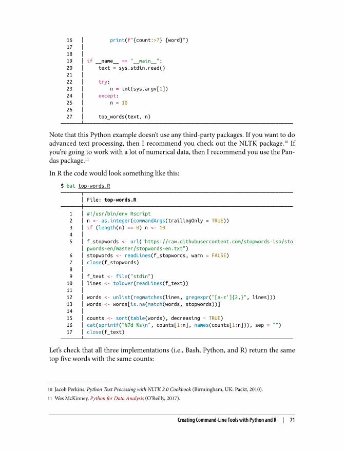
10 Jacob Perkins, Python Text Processing with NLTK 2.0 Cookbook (Birmingham, UK: Packt, 2010).11 Wes McKinney, Python for Data Analysis (O’Reilly, 2017).

16 │ print(f"{count:>7} {word}") 17 │ 18 │ 19 │ if __name__ == "__main__": 20 │ text = sys.stdin.read() 21 │ 22 │ try: 23 │ n = int(sys.argv[1]) 24 │ except: 25 │ n = 10 26 │ 27 │ top_words(text, n)───────┴────────────────────────────────────────────────────────────────────────

Note that this Python example doesn’t use any third-party packages. If you want to doadvanced text processing, then I recommend you check out the NLTK package.10 Ifyou’re going to work with a lot of numerical data, then I recommend you use the Pan‐das package.11

In R the code would look something like this:

$ bat top-words.R───────┬──────────────────────────────────────────────────────────────────────── │ File: top-words.R───────┼──────────────────────────────────────────────────────────────────────── 1 │ #!/usr/bin/env Rscript 2 │ n <- as.integer(commandArgs(trailingOnly = TRUE)) 3 │ if (length(n) == 0) n <- 10 4 │ 5 │ f_stopwords <- url("https://raw.githubusercontent.com/stopwords-iso/sto │ pwords-en/master/stopwords-en.txt") 6 │ stopwords <- readLines(f_stopwords, warn = FALSE) 7 │ close(f_stopwords) 8 │ 9 │ f_text <- file("stdin") 10 │ lines <- tolower(readLines(f_text)) 11 │ 12 │ words <- unlist(regmatches(lines, gregexpr("[a-z']{2,}", lines))) 13 │ words <- words[is.na(match(words, stopwords))] 14 │ 15 │ counts <- sort(table(words), decreasing = TRUE) 16 │ cat(sprintf("%7d %s\n", counts[1:n], names(counts[1:n])), sep = "") 17 │ close(f_text)───────┴────────────────────────────────────────────────────────────────────────

Let’s check that all three implementations (i.e., Bash, Python, and R) return the sametop five words with the same counts:

Creating Command-Line Tools with Python and R | 71

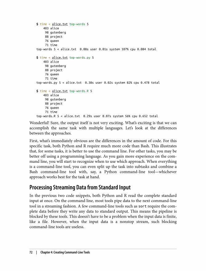
$ time < alice.txt top-words 5 403 alice 98 gutenberg 88 project 76 queen 71 timetop-words 5 < alice.txt 0.08s user 0.01s system 107% cpu 0.084 total $ time < alice.txt top-words.py 5 403 alice 98 gutenberg 88 project 76 queen 71 timetop-words.py 5 < alice.txt 0.38s user 0.02s system 82% cpu 0.478 total $ time < alice.txt top-words.R 5 403 alice 98 gutenberg 88 project 76 queen 71 timetop-words.R 5 < alice.txt 0.29s user 0.07s system 56% cpu 0.652 total

Wonderful! Sure, the output itself is not very exciting. What’s exciting is that we canaccomplish the same task with multiple languages. Let’s look at the differencesbetween the approaches.

First, what’s immediately obvious are the differences in the amount of code. For thisspecific task, both Python and R require much more code than Bash. This illustratesthat, for some tasks, it is better to use the command line. For other tasks, you may bebetter off using a programming language. As you gain more experience on the com‐mand line, you will start to recognize when to use which approach. When everythingis a command-line tool, you can even split up the task into subtasks and combine aBash command-line tool with, say, a Python command-line tool—whicheverapproach works best for the task at hand.

Processing Streaming Data from Standard InputIn the previous two code snippets, both Python and R read the complete standardinput at once. On the command line, most tools pipe data to the next command-linetool in a streaming fashion. A few command-line tools such as sort require the com‐plete data before they write any data to standard output. This means the pipeline isblocked by these tools. This doesn’t have to be a problem when the input data is finite,like a file. However, when the input data is a nonstop stream, such blockingcommand-line tools are useless.

72 | Chapter 4: Creating Command-Line Tools

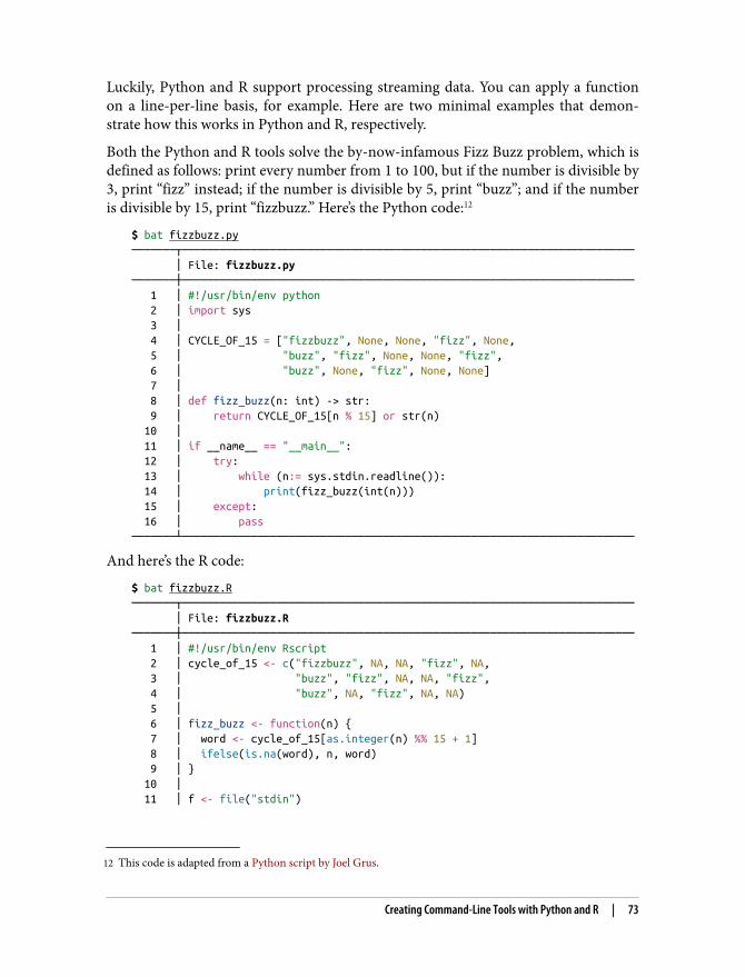
12 This code is adapted from a Python script by Joel Grus.

Luckily, Python and R support processing streaming data. You can apply a functionon a line-per-line basis, for example. Here are two minimal examples that demon‐strate how this works in Python and R, respectively.

Both the Python and R tools solve the by-now-infamous Fizz Buzz problem, which isdefined as follows: print every number from 1 to 100, but if the number is divisible by3, print “fizz” instead; if the number is divisible by 5, print “buzz”; and if the numberis divisible by 15, print “fizzbuzz.” Here’s the Python code:12

$ bat fizzbuzz.py───────┬──────────────────────────────────────────────────────────────────────── │ File: fizzbuzz.py───────┼──────────────────────────────────────────────────────────────────────── 1 │ #!/usr/bin/env python 2 │ import sys 3 │ 4 │ CYCLE_OF_15 = ["fizzbuzz", None, None, "fizz", None, 5 │ "buzz", "fizz", None, None, "fizz", 6 │ "buzz", None, "fizz", None, None] 7 │ 8 │ def fizz_buzz(n: int) -> str: 9 │ return CYCLE_OF_15[n % 15] or str(n) 10 │ 11 │ if __name__ == "__main__": 12 │ try: 13 │ while (n:= sys.stdin.readline()): 14 │ print(fizz_buzz(int(n))) 15 │ except: 16 │ pass───────┴────────────────────────────────────────────────────────────────────────

And here’s the R code:

$ bat fizzbuzz.R───────┬──────────────────────────────────────────────────────────────────────── │ File: fizzbuzz.R───────┼──────────────────────────────────────────────────────────────────────── 1 │ #!/usr/bin/env Rscript 2 │ cycle_of_15 <- c("fizzbuzz", NA, NA, "fizz", NA, 3 │ "buzz", "fizz", NA, NA, "fizz", 4 │ "buzz", NA, "fizz", NA, NA) 5 │ 6 │ fizz_buzz <- function(n) { 7 │ word <- cycle_of_15[as.integer(n) %% 15 + 1] 8 │ ifelse(is.na(word), n, word) 9 │ } 10 │ 11 │ f <- file("stdin")

Creating Command-Line Tools with Python and R | 73

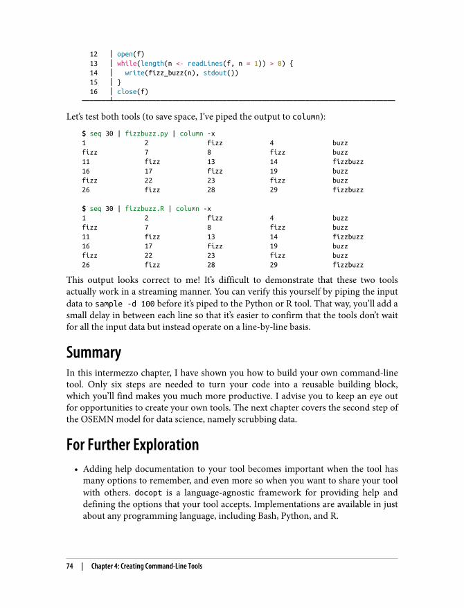
12 │ open(f) 13 │ while(length(n <- readLines(f, n = 1)) > 0) { 14 │ write(fizz_buzz(n), stdout()) 15 │ } 16 │ close(f)───────┴────────────────────────────────────────────────────────────────────────

Let’s test both tools (to save space, I’ve piped the output to column):

$ seq 30 | fizzbuzz.py | column -x1 2 fizz 4 buzzfizz 7 8 fizz buzz11 fizz 13 14 fizzbuzz16 17 fizz 19 buzzfizz 22 23 fizz buzz26 fizz 28 29 fizzbuzz $ seq 30 | fizzbuzz.R | column -x1 2 fizz 4 buzzfizz 7 8 fizz buzz11 fizz 13 14 fizzbuzz16 17 fizz 19 buzzfizz 22 23 fizz buzz26 fizz 28 29 fizzbuzz

This output looks correct to me! It’s difficult to demonstrate that these two toolsactually work in a streaming manner. You can verify this yourself by piping the inputdata to sample -d 100 before it’s piped to the Python or R tool. That way, you’ll add asmall delay in between each line so that it’s easier to confirm that the tools don’t waitfor all the input data but instead operate on a line-by-line basis.

SummaryIn this intermezzo chapter, I have shown you how to build your own command-linetool. Only six steps are needed to turn your code into a reusable building block,which you’ll find makes you much more productive. I advise you to keep an eye outfor opportunities to create your own tools. The next chapter covers the second step ofthe OSEMN model for data science, namely scrubbing data.

For Further Exploration• Adding help documentation to your tool becomes important when the tool has

many options to remember, and even more so when you want to share your toolwith others. docopt is a language-agnostic framework for providing help anddefining the options that your tool accepts. Implementations are available in justabout any programming language, including Bash, Python, and R.

74 | Chapter 4: Creating Command-Line Tools

• If you want to learn more about programming in Bash, I recommend ClassicShell Programming by Arnold Robbins and Nelson H. F. Beebe (O’Reilly) andBash Cookbook, 2nd Edition by Carl Albing and JP Vossen (O’Reilly).

• Writing a robust and safe Bash script is quite tricky. ShellCheck is an online toolthat will check your Bash code for mistakes and vulnerabilities. A command-linetool is also available.

• The book Ten Essays on Fizz Buzz by Joel Grus (Brightwalton) is an insightfuland fun collection of 10 different ways to solve Fizz Buzz with Python.

For Further Exploration | 75

1 Mike D. Brennan and Thomas E. Dickey, awk – Pattern Scanning and Text Processing Language, version 1.3.4,2019, https://invisible-island.net/mawk.

CHAPTER 5

Scrubbing Data

Two chapters ago, in the first step of the OSEMN model for data science, we looked atobtaining data from a variety of sources. This chapter is all about the second step:scrubbing data. You see, it’s quite rare that you can move directly from obtaining datato exploring or even modeling the data. There’s a plethora of reasons why your datafirst needs some cleaning, or scrubbing.

For starters, the data might not be in the desired format. For example, you may haveobtained some JSON data from an API, but you need it to be in CSV format to createa visualization. Other common formats include plain text, HTML, and XML. Mostcommand-line tools work with only one or two formats, so it’s important that you’reable to convert data from one format to another.

Once the data is in the desired format, there could still be issues like missing values,inconsistencies, weird characters, or unnecessary parts. You can fix these by applyingfilters, replacing values, and combining multiple files. The command line is especiallywell suited for these kind of transformations, because there are many specialized toolsavailable, most of which can handle large amounts of data. In this chapter I’ll discussclassic tools such as grep and awk,1 and newer tools such as jq and pup.

Sometimes you can use the same command-line tool to perform several operations ormultiple tools to perform the same operation. This chapter is structured more like acookbook in that it focuses on the problems or recipes rather than diving deeply intothe command-line tools themselves.

77

OverviewIn this chapter, you’ll learn how to:

• Convert data from one format to another• Apply SQL queries directly to CSV• Filter lines• Extract and replace values• Split, merge, and extract columns• Combine multiple files

This chapter starts with the following files:

$ cd /data/ch05 $ ltotal 200K-rw-r--r-- 1 dst dst 164K Jun 29 14:28 alice.txt-rw-r--r-- 1 dst dst 4.5K Jun 29 14:28 iris.csv-rw-r--r-- 1 dst dst 179 Jun 29 14:28 irismeta.csv-rw-r--r-- 1 dst dst 160 Jun 29 14:28 names-comma.csv-rw-r--r-- 1 dst dst 129 Jun 29 14:28 names.csv-rw-r--r-- 1 dst dst 7.8K Jun 29 14:28 tips.csv-rw-r--r-- 1 dst dst 5.1K Jun 29 14:28 users.json

The instructions for getting these files are in Chapter 2. Any other files are eitherdownloaded or generated using command-line tools.

Before I dive into the actual transformations, I’d like to demonstrate their ubiquitywhen working at the command line.

Transformations, Transformations EverywhereIn Chapter 1 I mentioned that, in practice, the steps of the OSEMN model will rarelybe followed linearly. In this vein, although scrubbing is the second step of theOSEMN model, I want you to know that it’s not just the obtained data that needsscrubbing. The transformations that you’ll learn in this chapter can be useful at anypart of your pipeline and at any step of the OSEMN model. Generally, if onecommand-line tool generates output that can be used immediately by the next tool,you can chain the two tools together by using the pipe operator (|). Otherwise, atransformation first needs to be applied to the data by inserting an intermediate toolinto the pipeline.

78 | Chapter 5: Scrubbing Data

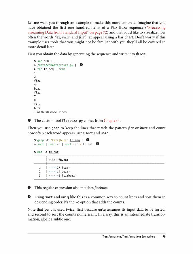
Let me walk you through an example to make this more concrete. Imagine that youhave obtained the first one hundred items of a Fizz Buzz sequence (“ProcessingStreaming Data from Standard Input” on page 72) and that you’d like to visualize howoften the words fizz, buzz, and fizzbuzz appear using a bar chart. Don’t worry if thisexample uses tools that you might not be familiar with yet; they’ll all be covered inmore detail later.

First you obtain the data by generating the sequence and write it to fb.seq:

$ seq 100 |> /data/ch04/fizzbuzz.py | > tee fb.seq | trim12fizz4buzzfizz78fizzbuzz… with 90 more lines

The custom tool fizzbuzz.py comes from Chapter 4.

Then you use grep to keep the lines that match the pattern fizz or buzz and counthow often each word appears using sort and uniq:

$ grep -E "fizz|buzz" fb.seq | > sort | uniq -c | sort -nr > fb.cnt $ bat -A fb.cnt───────┬──────────────────────────────────────────────────────────────────────── │ File: fb.cnt───────┼──────────────────────────────────────────────────────────────────────── 1 │ ·····27·fizz␊ 2 │ ·····14·buzz␊ 3 │ ······6·fizzbuzz␊───────┴────────────────────────────────────────────────────────────────────────

This regular expression also matches fizzbuzz.

Using sort and uniq like this is a common way to count lines and sort them indescending order. It’s the -c option that adds the counts.

Note that sort is used twice: first because uniq assumes its input data to be sorted,and second to sort the counts numerically. In a way, this is an intermediate transfor‐mation, albeit a subtle one.

Transformations, Transformations Everywhere | 79

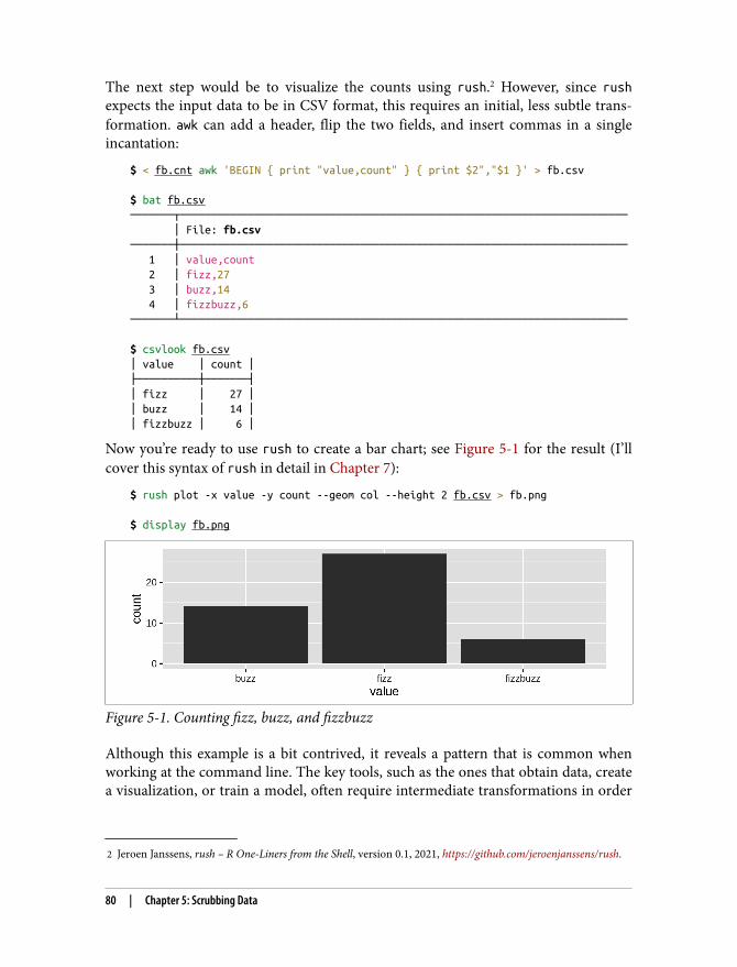
2 Jeroen Janssens, rush – R One-Liners from the Shell, version 0.1, 2021, https://github.com/jeroenjanssens/rush.

The next step would be to visualize the counts using rush.2 However, since rushexpects the input data to be in CSV format, this requires an initial, less subtle trans‐formation. awk can add a header, flip the two fields, and insert commas in a singleincantation:

$ < fb.cnt awk 'BEGIN { print "value,count" } { print $2","$1 }' > fb.csv $ bat fb.csv───────┬──────────────────────────────────────────────────────────────────────── │ File: fb.csv───────┼──────────────────────────────────────────────────────────────────────── 1 │ value,count 2 │ fizz,27 3 │ buzz,14 4 │ fizzbuzz,6───────┴──────────────────────────────────────────────────────────────────────── $ csvlook fb.csv│ value │ count │├──────────┼───────┤│ fizz │ 27 ││ buzz │ 14 ││ fizzbuzz │ 6 │

Now you’re ready to use rush to create a bar chart; see Figure 5-1 for the result (I’llcover this syntax of rush in detail in Chapter 7):

$ rush plot -x value -y count --geom col --height 2 fb.csv > fb.png $ display fb.png

Figure 5-1. Counting fizz, buzz, and fizzbuzz

Although this example is a bit contrived, it reveals a pattern that is common whenworking at the command line. The key tools, such as the ones that obtain data, createa visualization, or train a model, often require intermediate transformations in order

80 | Chapter 5: Scrubbing Data

3 The Linux Information Project, “Plain Text Definition,” last updated February 9, 2007, http://www.linfo.org/plain_text.html.

4 Andrew Hunt and David Thomas, The Pragmatic Programmer (Reading, MA: Addison-Wesley, 1999).5 Raymond, The Art of Unix Programming.

to be chained into a pipeline. In that sense, writing a pipeline is like solving a puzzle,where the key pieces often require helper pieces to fit.

Now that you’ve seen the importance of scrubbing data, you’re ready to learn aboutsome actual transformations.

Plain TextFormally speaking, plain text refers to a sequence of human-readable characters and,optionally, some specific types of control characters such as tabs and newlines.3

Examples are logs, ebooks, emails, and source code. Plain text has many advantagesover binary data, including the following:4

• It can be opened, edited, and saved using any text editor.• It’s self-describing and independent of the application that created it.• It will outlive other forms of data, because no additional knowledge or applica‐

tions are required to process it.

Most importantly, the Unix philosophy considers plain text to be the universal inter‐face between command-line tools.5 This means that most tools accept plain text asinput and produce plain text as output.

That’s reason enough for me to start with plain text. The other formats that I discussin this chapter—CSV, JSON, XML, and HTML—are indeed also plain text. For now, Iassume that the plain text has no clear tabular structure (like CSV does) or nestedstructure (like JSON, XML, and HTML do). Later in this chapter, I’ll introduce sometools that are specifically designed for working with these formats.

Filtering LinesThe first scrubbing operation is filtering lines. This means that each line from theinput data will be evaluated on whether it will be kept or discarded.

Based on locationThe most straightforward way to filter lines is based on their location. This may beuseful when you want to inspect, say, the top 10 lines of a file, or when you extract a

Plain Text | 81

6 Jay Fenlason et al., sed – Stream Editor for Filtering and Transforming Text, version 4.7, 2018, https://www.gnu.org/software/sed.

7 Paul Rubin et al., tail – Output the Last Part of Files, version 8.30, 2019, https://www.gnu.org/software/coreutils.

specific row from the output of another command-line tool. To illustrate how to filterbased on location, let’s create a file that contains 10 lines:

$ seq -f "Line %g" 10 | tee linesLine 1Line 2Line 3Line 4Line 5Line 6Line 7Line 8Line 9Line 10

You can print the first three lines using either head, sed,6 or awk:

$ < lines head -n 3Line 1Line 2Line 3 $ < lines sed -n '1,3p'Line 1Line 2Line 3 $ < lines awk 'NR <= 3' Line 1Line 2Line 3

In awk, NR refers to the total number of input records seen so far.

Similarly, you can print the last three lines using tail:7

$ < lines tail -n 3Line 8Line 9Line 10

You can also you use sed and awk for this, but tail is much faster. Removing the firstthree lines goes as follows:

$ < lines tail -n +4Line 4Line 5

82 | Chapter 5: Scrubbing Data

Line 6Line 7Line 8Line 9Line 10 $ < lines sed '1,3d'Line 4Line 5Line 6Line 7Line 8Line 9Line 10 $ < lines sed -n '1,3!p'Line 4Line 5Line 6Line 7Line 8Line 9Line 10

Notice that with tail you have to specify the number of lines you want to removeplus one. Think of it as the line from which you want to start printing. Removing thelast three lines can be done with head:

$ < lines head -n -3Line 1Line 2Line 3Line 4Line 5Line 6Line 7

You can print specific lines using either sed, awk, or a combination of head and tail.Here I print lines 4, 5, and 6:

$ < lines sed -n '4,6p'Line 4Line 5Line 6 $ < lines awk '(NR>=4) && (NR<=6)'Line 4Line 5Line 6 $ < lines head -n 6 | tail -n 3Line 4

Plain Text | 83

Line 5Line 6

You can print odd lines with sed by specifying a start and a step, or with awk by usingthe modulo operator:

$ < lines sed -n '1~2p'Line 1Line 3Line 5Line 7Line 9 $ < lines awk 'NR%2'Line 1Line 3Line 5Line 7Line 9

Printing even lines works in a similar manner:

$ < lines sed -n '0~2p'Line 2Line 4Line 6Line 8Line 10 $ < lines awk '(NR+1)%2'Line 2Line 4Line 6Line 8Line 10

Many of these examples start with the less-than sign (<) followedby the filename. I do this because it allows me to read the pipelinefrom left to right. Please know that this is my own preference. Youcan also use cat to pipe the contents of a file. Additionally, manycommand-line tools accept the filename as an argument.

Based on a pattern

Sometimes you want to keep or discard lines based on their contents. With grep, thecanonical command-line tool for filtering lines, you can print every line that matchesa certain pattern or regular expression. For example, to extract all the chapter head‐ings from Alice’s Adventures in Wonderland:

$ < alice.txt grep -i chapter CHAPTER I. Down the Rabbit-Hole

84 | Chapter 5: Scrubbing Data

8 Jeroen Janssens, sample – Filter Lines from Standard Input According to Some Probability, with a Given Delay,and for a Certain Duration, version 0.2.4, 2021, https://github.com/jeroenjanssens/sample.

CHAPTER II. The Pool of TearsCHAPTER III. A Caucus-Race and a Long TaleCHAPTER IV. The Rabbit Sends in a Little BillCHAPTER V. Advice from a CaterpillarCHAPTER VI. Pig and PepperCHAPTER VII. A Mad Tea-PartyCHAPTER VIII. The Queen's Croquet-GroundCHAPTER IX. The Mock Turtle's StoryCHAPTER X. The Lobster QuadrilleCHAPTER XI. Who Stole the Tarts?CHAPTER XII. Alice's Evidence

The -i option specifies that the matching should be case insensitive.

You can also specify a regular expression. For example, if you wanted to print onlythe headings that start with The:

$ < alice.txt grep -E '^CHAPTER (.*)\. The'CHAPTER II. The Pool of TearsCHAPTER IV. The Rabbit Sends in a Little BillCHAPTER VIII. The Queen's Croquet-GroundCHAPTER IX. The Mock Turtle's StoryCHAPTER X. The Lobster Quadrille

Note that you have to specify the -E option to enable regular expressions. Otherwise,grep interprets the pattern as a literal string, which most likely results in no matchesat all:

$ < alice.txt grep '^CHAPTER (.*)\. The'

With the -v option, you invert the matches, so that grep prints the lines that don’tmatch the pattern. The regular expression below matches lines that contain whitespace only. So with the inverse, and using wc -l, you can count the number of non-empty lines:

$ < alice.txt grep -Ev '^\s$' | wc -l2790

Based on randomnessWhen you’re in the process of formulating your data pipeline and you have a lot ofdata, debugging your pipeline can be cumbersome. In that case, generating a smallersample from the data might be useful. This is where sample8 comes in handy. Themain purpose of sample is to get a subset of the data by outputting only a certain per‐centage of the input on a line-by-line basis:

Plain Text | 85

9 Joey Hess, ts – Timestamp Input, version 0.65, 2021, https://joeyh.name/code/moreutils.10 David M. Ihnat, David MacKenzie, and Jim Meyering, cut – Remove Sections from Each Line of Files, version

8.30, 2019, https://www.gnu.org/software/coreutils.

$ seq -f "Line %g" 1000 | sample -r 1%Line 50Line 159Line 173Line 682Line 882Line 921Line 986

Here, every input line has a 1% chance of being printed. This percentage can also bespecified as a fraction (namely 1/100) or as a probability (namely 0.01).

sample has two other purposes that can be useful when you’re debugging your pipe‐line. First, it’s possible to add some delay to the output. This comes in handy whenthe input is a constant stream (for example, the Wikipedia stream we saw in Chap‐ter 3), and the data comes in too fast for you to see what’s going on. Second, you canput a timer on sample so that you don’t have to kill the ongoing process manually. Forexample, to add a one-second delay between each line being printed and to run foronly five seconds, you would type:

$ seq -f "Line %g" 1000 | sample -r 1% -d 1000 -s 5 | ts Jun 29 14:28:50 Line 28Jun 29 14:28:51 Line 262Jun 29 14:28:52 Line 324Jun 29 14:28:53 Line 546Jun 29 14:28:54 Line 589Jun 29 14:28:55 Line 613Jun 29 14:28:56 Line 629

The tool ts9 adds a timestamp in front of each line.

To prevent unnecessary computation, try to put sample as early as possible in yourpipeline. In fact, this argument holds for any command-line tool that reduces data,like head and tail. Once you’re confident your pipeline works, you take the tool outof the pipeline.

Extracting ValuesTo extract the actual chapter headings from our earlier example, you can take a sim‐ple approach by piping the output of grep to cut:10

$ grep -i chapter alice.txt | cut -d ' ' -f 3-Down the Rabbit-HoleThe Pool of Tears

86 | Chapter 5: Scrubbing Data

A Caucus-Race and a Long TaleThe Rabbit Sends in a Little BillAdvice from a CaterpillarPig and PepperA Mad Tea-PartyThe Queen's Croquet-GroundThe Mock Turtle's StoryThe Lobster QuadrilleWho Stole the Tarts?Alice's Evidence

Here, each line that’s passed to cut is being split on spaces into fields, and then thethird field to the last field is being printed. The total number of fields can be differentper input line. With sed you can accomplish the same task in a much more complexmanner:

$ sed -rn 's/^CHAPTER ([IVXLCDM]{1,})\. (.*)$/\2/p' alice.txt | trim 3Down the Rabbit-HoleThe Pool of TearsA Caucus-Race and a Long Tale… with 9 more lines

This approach uses a regular expression and a back reference. Here, sed also takesover the work done by grep. I recommend using such a complicated approach onlywhen a simpler one would not work—for example, if chapter was ever part of the textitself and not just used to indicate the start of a new chapter. Of course, there aremany levels of complexity that would have worked around this, but this is intended toillustrate an extremely strict approach. In practice, the challenge is to come up with apipeline that strikes a good balance between complexity and flexibility.

It’s worth noting that cut can also split on characters’ positions. This is useful forwhen you want to extract (or remove) the same set of characters per input line:

$ grep -i chapter alice.txt | cut -c 9-I. Down the Rabbit-HoleII. The Pool of TearsIII. A Caucus-Race and a Long TaleIV. The Rabbit Sends in a Little BillV. Advice from a CaterpillarVI. Pig and PepperVII. A Mad Tea-PartyVIII. The Queen's Croquet-GroundIX. The Mock Turtle's StoryX. The Lobster QuadrilleXI. Who Stole the Tarts?XII. Alice's Evidence

grep has a great feature that outputs every match onto a separate line using the -ooption:

Plain Text | 87

$ < alice.txt grep -oE '\w{2,}' | trimProjectGutenbergAliceAdventuresinWonderlandbyLewisCarrollThis… with 28615 more lines

But what if you wanted to create a dataset of all the words that start with an a and endwith an e? Well, of course there’s a pipeline for that too:

$ < alice.txt tr '[:upper:]' '[:lower:]' | > grep -oE '\w{2,}' |> grep -E '^a.*e$' |> sort | uniq | sort -nr | trimavailableateassistanceaskancearisearguearearchiveapplicableapple… with 25 more lines

I use tr here to make the text lowercase. We’ll have a closer look at tr in the nextsection.

The two grep commands might have been combined into one, but in this case Idecided it would be easier to reuse and adapt the previous pipeline. There’s no shamein being pragmatic to get the job done!

Replacing and Deleting ValuesYou can use the command-line tool tr, which stands for translate, to replace or deleteindividual characters. For example, spaces can be replaced by underscores as follows:

$ echo 'hello world!' | tr ' ' '_'hello_world!

If more than one character needs to be replaced, then you can combine thoserequests:

$ echo 'hello world!' | tr ' !' '_?'hello_world?

88 | Chapter 5: Scrubbing Data

tr can also be used to delete individual characters by specifying the argument -d:

$ echo 'hello world!' | tr -d ' !'helloworld $ echo 'hello world!' | tr -d -c '[a-z]'helloworld%

In this case, these two commands accomplish the same thing. The second command,however, uses two additional features: it specifies a range of characters (all lowercaseletters) using the square brackets and the dash ([-]), and the -c option indicates thatthe complement of that should be used. In other words, this command keeps onlylowercase letters. You can even use tr to convert text to uppercase:

$ echo 'hello world!' | tr '[a-z]' '[A-Z]'HELLO WORLD! $ echo 'hello world!' | tr '[:lower:]' '[:upper:]'HELLO WORLD!

However, if you need to translate non-ASCII characters, then tr may not workbecause it operates on single-byte characters only. In those cases, you should use sedinstead:

$ echo 'hello world!' | tr '[a-z]' '[A-Z]'HELLO WORLD! $ echo 'hallo wêreld!' | tr '[a-z]' '[A-Z]'HALLO WêRELD! $ echo 'hallo wêreld!' | tr '[:lower:]' '[:upper:]'HALLO WêRELD! $ echo 'hallo wêreld!' | sed 's/[[:lower:]]*/\U&/g'HALLO WÊRELD! $ echo 'helló világ' | tr '[:lower:]' '[:upper:]'HELLó VILáG $ echo 'helló világ' | sed 's/[[:lower:]]*/\U&/g'HELLÓ VILÁG

If you need to operate on more than individual characters, then you may find seduseful. You’ve already seen an example of sed being used to extract the chapter head‐ings from alice.txt. Extracting, deleting, and replacing are actually all the same opera‐tion in sed. You just specify different regular expressions. For example, to change aword, remove repeated spaces, and remove leading spaces:

$ echo ' hello world!' |> sed -re 's/hello/bye/' | > sed -re 's/\s+/ /g' |

Plain Text | 89

11 Jeroen Janssens, body – Apply Command to All but the First Line, version 0.1, 2021, https://github.com/jeroenjanssens/dsutils.

12 Jeroen Janssens, header – Add, Replace, and Delete Header Lines, version 0.1, 2021, https://github.com/jeroenjanssens/dsutils.

13 Jeroen Janssens, cols – Apply Command to Subset of Columns, version 0.1, 2021, https://github.com/jeroenjanssens/dsutils.

> sed -re 's/\s+//' bye world!

Replace hello with bye.

Replace any whitespace with one space. The flag g stands for global, meaning thatthe same substitution can be applied more than once on the same line.

This removes leading spaces only because I didn’t specify the flag g here.

Again, just as with the grep example earlier, these three sed commands can be com‐bined into one:

$ echo ' hello world!' |> sed -re 's/hello/bye/;s/\s+/ /g;s/\s+//'bye world!

But tell me—what do you find easier to read?

CSVThe command-line tools such as tr and grep that I’ve used to scrub plain text cannotalways be applied to CSV. The reason is that these command-line tools have nonotion of headers, bodies, and columns.

Bodies and Headers and Columns, Oh My!What if you want to filter lines using grep but always include the header in the out‐put? Or what if you want to uppercase the values of only a specific column using trand leave the other columns untouched?

There are multistep workarounds for this, but they are very cumbersome. I havesomething better. I’d like to introduce you to three command-line tools, aptly namedbody,11 header,12 and cols,13 that will enable you to leverage ordinary command-linetools for CSV.

Let’s start with the first tool, body. With body you can apply any command-line toolto the body of a CSV file—that is, to everything excluding the header. For example:

90 | Chapter 5: Scrubbing Data

$ echo -e "value\n7\n2\n5\n3" | body sort -nvalue2357

body assumes that the header of the CSV file spans only one row. It works like this:

• Take one line from standard input and store it as a variable named $header.• Print out the header.• Execute all the command-line arguments passed to body on the remaining data

in standard input.

Here’s another example. Imagine that you want to count the lines of the followingCSV file:

$ seq 5 | header -a countcount12345

With wc -l, you can count the number of all lines:

$ seq 5 | header -a count | wc -l6

If you want to consider only the lines in the body (i.e., everything except the header),you add body:

$ seq 5 | header -a count | body wc -lcount5

Note that the header is not used and is also printed again in the output.

The second command-line tool, header, allows you to manipulate the header of aCSV file. If no arguments are provided, the header of the CSV file is printed:

$ < tips.csv headerbill,tip,sex,smoker,day,time,size

This is the same as head -n 1. If the header spans more than one row, which is notrecommended, you can specify -n 2. You can also add a header to a CSV file:

$ seq 5 | header -a countcount12

CSV | 91

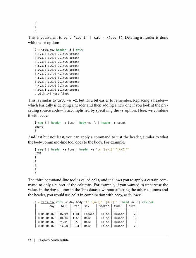
345

This is equivalent to echo "count" | cat - <(seq 5). Deleting a header is donewith the -d option:

$ < iris.csv header -d | trim5.1,3.5,1.4,0.2,Iris-setosa4.9,3.0,1.4,0.2,Iris-setosa4.7,3.2,1.3,0.2,Iris-setosa4.6,3.1,1.5,0.2,Iris-setosa5.0,3.6,1.4,0.2,Iris-setosa5.4,3.9,1.7,0.4,Iris-setosa4.6,3.4,1.4,0.3,Iris-setosa5.0,3.4,1.5,0.2,Iris-setosa4.4,2.9,1.4,0.2,Iris-setosa4.9,3.1,1.5,0.1,Iris-setosa… with 140 more lines

This is similar to tail -n +2, but it’s a bit easier to remember. Replacing a header—which basically is deleting a header and then adding a new one if you look at the pre‐ceding source code—is accomplished by specifying the -r option. Here, we combineit with body:

$ seq 5 | header -a line | body wc -l | header -r countcount5

And last but not least, you can apply a command to just the header, similar to whatthe body command-line tool does to the body. For example:

$ seq 5 | header -a line | header -e "tr '[a-z]' '[A-Z]'"LINE12345

The third command-line tool is called cols, and it allows you to apply a certain com‐mand to only a subset of the columns. For example, if you wanted to uppercase thevalues in the day column in the Tips dataset without affecting the other columns andthe header, you would use cols in combination with body, as follows:

$ < tips.csv cols -c day body "tr '[a-z]' '[A-Z]'" | head -n 5 | csvlook│ day │ bill │ tip │ sex │ smoker │ time │ size │├────────────┼───────┼──────┼────────┼────────┼────────┼──────┤│ 0001-01-07 │ 16.99 │ 1.01 │ Female │ False │ Dinner │ 2 ││ 0001-01-07 │ 10.34 │ 1.66 │ Male │ False │ Dinner │ 3 ││ 0001-01-07 │ 21.01 │ 3.50 │ Male │ False │ Dinner │ 3 ││ 0001-01-07 │ 23.68 │ 3.31 │ Male │ False │ Dinner │ 2 │

92 | Chapter 5: Scrubbing Data

14 Christopher Groskopf, csvsql – Execute SQL Statements on CSV Files, version 1.0.5, 2020, https://csvkit.rtfd.org.

Please note that passing multiple command-line tools and arguments as commandsto header -e, body, and cols can lead to tricky quoting citations. If you ever run intosuch problems, it’s best to create a separate command-line tool for this and pass it ascommand.

In conclusion, while it is generally preferable to use command-line tools that aremade specifically for CSV data, body, header, and cols also allow you to apply theclassic command-line tools to CSV files if needed.

Performing SQL Queries on CSVIn case the command-line tools mentioned in this chapter do not provide enoughflexibility, there is another approach to scrubbing your data from the command line.The tool csvsql14 allows you to execute SQL queries directly on CSV files. SQL is apowerful language for defining operations for scrubbing data; it’s a very differentapproach from using individual command-line tools.

If your data originally comes from a relational database, then, ifpossible, try to execute SQL queries on that database and subse‐quently extract the data as CSV. As I discussed in Chapter 3, youcan use the command-line tool sql2csv for this. When you firstexport data from the database to a CSV file and then apply SQL,not only is it slower, but there is also a possibility that the columntypes will not be correctly inferred from the CSV data.

In the following scrubbing tasks, I’ll include several solutions that involve csvsql. Abasic command is this:

$ seq 5 | header -a val | csvsql --query "SELECT SUM(val) AS sum FROM stdin"sum15.0

If you pass standard input to csvsql, then the table is named stdin. The types of thecolumn are automatically inferred from the data. As you’ll see later in “CombiningMultiple CSV Files” on page 99, you can also specify multiple CSV files. Please keepin mind that csvsql employs the SQLite dialect of SQL, which has some subtle differ‐ences with respect to the SQL standard. While SQL is generally more verbose thanthe other solutions, it is also much more flexible. If you already know how to tackle ascrubbing problem with SQL, then why not use it when you’re at the command line?

CSV | 93

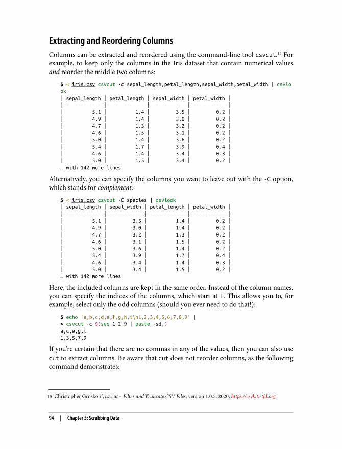
15 Christopher Groskopf, csvcut – Filter and Truncate CSV Files, version 1.0.5, 2020, https://csvkit.rtfd.org.

Extracting and Reordering ColumnsColumns can be extracted and reordered using the command-line tool csvcut.15 Forexample, to keep only the columns in the Iris dataset that contain numerical valuesand reorder the middle two columns:

$ < iris.csv csvcut -c sepal_length,petal_length,sepal_width,petal_width | csvlook│ sepal_length │ petal_length │ sepal_width │ petal_width │├──────────────┼──────────────┼─────────────┼─────────────┤│ 5.1 │ 1.4 │ 3.5 │ 0.2 ││ 4.9 │ 1.4 │ 3.0 │ 0.2 ││ 4.7 │ 1.3 │ 3.2 │ 0.2 ││ 4.6 │ 1.5 │ 3.1 │ 0.2 ││ 5.0 │ 1.4 │ 3.6 │ 0.2 ││ 5.4 │ 1.7 │ 3.9 │ 0.4 ││ 4.6 │ 1.4 │ 3.4 │ 0.3 ││ 5.0 │ 1.5 │ 3.4 │ 0.2 │… with 142 more lines

Alternatively, you can specify the columns you want to leave out with the -C option,which stands for complement:

$ < iris.csv csvcut -C species | csvlook│ sepal_length │ sepal_width │ petal_length │ petal_width │├──────────────┼─────────────┼──────────────┼─────────────┤│ 5.1 │ 3.5 │ 1.4 │ 0.2 ││ 4.9 │ 3.0 │ 1.4 │ 0.2 ││ 4.7 │ 3.2 │ 1.3 │ 0.2 ││ 4.6 │ 3.1 │ 1.5 │ 0.2 ││ 5.0 │ 3.6 │ 1.4 │ 0.2 ││ 5.4 │ 3.9 │ 1.7 │ 0.4 ││ 4.6 │ 3.4 │ 1.4 │ 0.3 ││ 5.0 │ 3.4 │ 1.5 │ 0.2 │… with 142 more lines

Here, the included columns are kept in the same order. Instead of the column names,you can specify the indices of the columns, which start at 1. This allows you to, forexample, select only the odd columns (should you ever need to do that!):

$ echo 'a,b,c,d,e,f,g,h,i\n1,2,3,4,5,6,7,8,9' |> csvcut -c $(seq 1 2 9 | paste -sd,)a,c,e,g,i1,3,5,7,9

If you’re certain that there are no commas in any of the values, then you can also usecut to extract columns. Be aware that cut does not reorder columns, as the followingcommand demonstrates:

94 | Chapter 5: Scrubbing Data

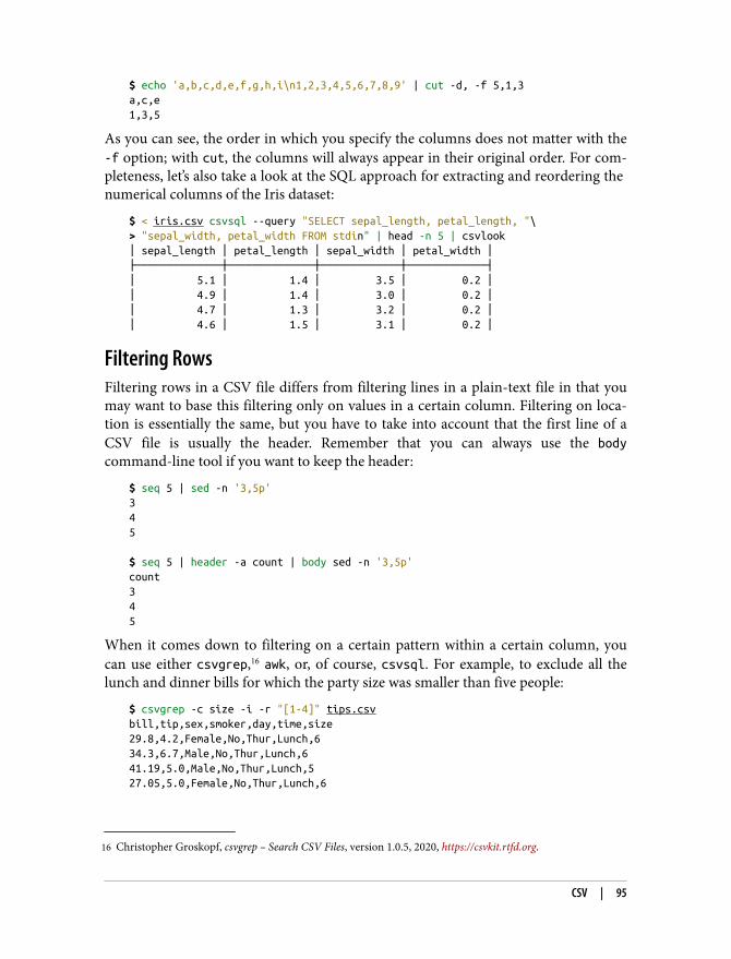
16 Christopher Groskopf, csvgrep – Search CSV Files, version 1.0.5, 2020, https://csvkit.rtfd.org.

$ echo 'a,b,c,d,e,f,g,h,i\n1,2,3,4,5,6,7,8,9' | cut -d, -f 5,1,3a,c,e1,3,5

As you can see, the order in which you specify the columns does not matter with the-f option; with cut, the columns will always appear in their original order. For com‐pleteness, let’s also take a look at the SQL approach for extracting and reordering the numerical columns of the Iris dataset:

$ < iris.csv csvsql --query "SELECT sepal_length, petal_length, "\> "sepal_width, petal_width FROM stdin" | head -n 5 | csvlook│ sepal_length │ petal_length │ sepal_width │ petal_width │├──────────────┼──────────────┼─────────────┼─────────────┤│ 5.1 │ 1.4 │ 3.5 │ 0.2 ││ 4.9 │ 1.4 │ 3.0 │ 0.2 ││ 4.7 │ 1.3 │ 3.2 │ 0.2 ││ 4.6 │ 1.5 │ 3.1 │ 0.2 │

Filtering RowsFiltering rows in a CSV file differs from filtering lines in a plain-text file in that youmay want to base this filtering only on values in a certain column. Filtering on loca‐tion is essentially the same, but you have to take into account that the first line of aCSV file is usually the header. Remember that you can always use the bodycommand-line tool if you want to keep the header:

$ seq 5 | sed -n '3,5p'345 $ seq 5 | header -a count | body sed -n '3,5p'count345

When it comes down to filtering on a certain pattern within a certain column, youcan use either csvgrep,16 awk, or, of course, csvsql. For example, to exclude all thelunch and dinner bills for which the party size was smaller than five people:

$ csvgrep -c size -i -r "[1-4]" tips.csvbill,tip,sex,smoker,day,time,size29.8,4.2,Female,No,Thur,Lunch,634.3,6.7,Male,No,Thur,Lunch,641.19,5.0,Male,No,Thur,Lunch,527.05,5.0,Female,No,Thur,Lunch,6

CSV | 95

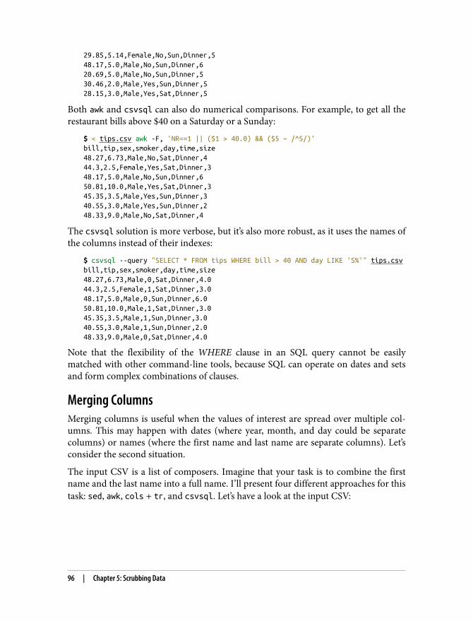
29.85,5.14,Female,No,Sun,Dinner,548.17,5.0,Male,No,Sun,Dinner,620.69,5.0,Male,No,Sun,Dinner,530.46,2.0,Male,Yes,Sun,Dinner,528.15,3.0,Male,Yes,Sat,Dinner,5

Both awk and csvsql can also do numerical comparisons. For example, to get all therestaurant bills above $40 on a Saturday or a Sunday:

$ < tips.csv awk -F, 'NR==1 || ($1 > 40.0) && ($5 ~ /^S/)'bill,tip,sex,smoker,day,time,size48.27,6.73,Male,No,Sat,Dinner,444.3,2.5,Female,Yes,Sat,Dinner,348.17,5.0,Male,No,Sun,Dinner,650.81,10.0,Male,Yes,Sat,Dinner,345.35,3.5,Male,Yes,Sun,Dinner,340.55,3.0,Male,Yes,Sun,Dinner,248.33,9.0,Male,No,Sat,Dinner,4

The csvsql solution is more verbose, but it’s also more robust, as it uses the names ofthe columns instead of their indexes:

$ csvsql --query "SELECT * FROM tips WHERE bill > 40 AND day LIKE 'S%'" tips.csvbill,tip,sex,smoker,day,time,size48.27,6.73,Male,0,Sat,Dinner,4.044.3,2.5,Female,1,Sat,Dinner,3.048.17,5.0,Male,0,Sun,Dinner,6.050.81,10.0,Male,1,Sat,Dinner,3.045.35,3.5,Male,1,Sun,Dinner,3.040.55,3.0,Male,1,Sun,Dinner,2.048.33,9.0,Male,0,Sat,Dinner,4.0

Note that the flexibility of the WHERE clause in an SQL query cannot be easilymatched with other command-line tools, because SQL can operate on dates and setsand form complex combinations of clauses.

Merging ColumnsMerging columns is useful when the values of interest are spread over multiple col‐umns. This may happen with dates (where year, month, and day could be separatecolumns) or names (where the first name and last name are separate columns). Let’sconsider the second situation.

The input CSV is a list of composers. Imagine that your task is to combine the firstname and the last name into a full name. I’ll present four different approaches for thistask: sed, awk, cols + tr, and csvsql. Let’s have a look at the input CSV:

96 | Chapter 5: Scrubbing Data

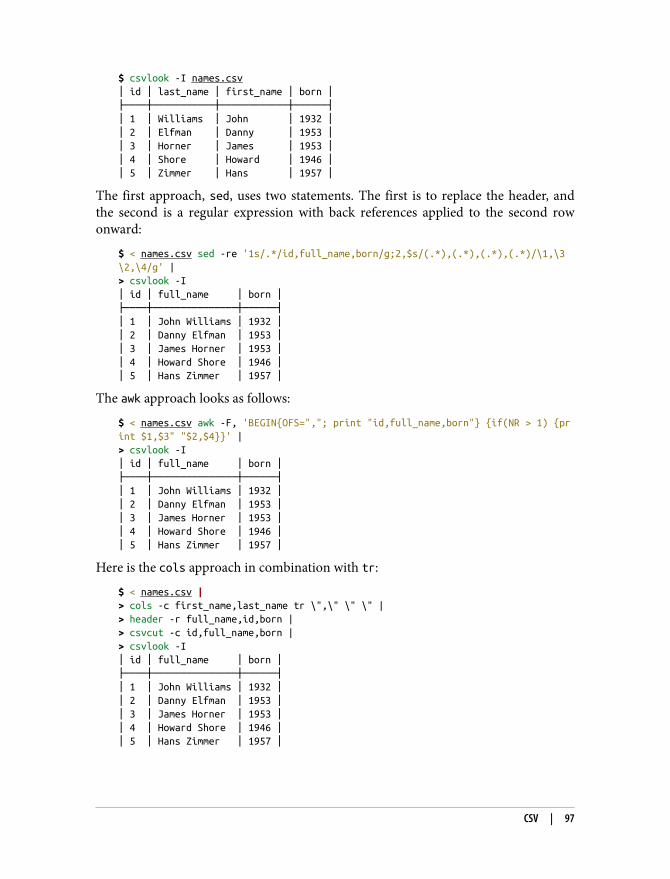
$ csvlook -I names.csv│ id │ last_name │ first_name │ born │├────┼───────────┼────────────┼──────┤│ 1 │ Williams │ John │ 1932 ││ 2 │ Elfman │ Danny │ 1953 ││ 3 │ Horner │ James │ 1953 ││ 4 │ Shore │ Howard │ 1946 ││ 5 │ Zimmer │ Hans │ 1957 │

The first approach, sed, uses two statements. The first is to replace the header, andthe second is a regular expression with back references applied to the second rowonward:

$ < names.csv sed -re '1s/.*/id,full_name,born/g;2,$s/(.*),(.*),(.*),(.*)/\1,\3\2,\4/g' |> csvlook -I│ id │ full_name │ born │├────┼───────────────┼──────┤│ 1 │ John Williams │ 1932 ││ 2 │ Danny Elfman │ 1953 ││ 3 │ James Horner │ 1953 ││ 4 │ Howard Shore │ 1946 ││ 5 │ Hans Zimmer │ 1957 │

The awk approach looks as follows:

$ < names.csv awk -F, 'BEGIN{OFS=","; print "id,full_name,born"} {if(NR > 1) {print $1,$3" "$2,$4}}' |> csvlook -I│ id │ full_name │ born │├────┼───────────────┼──────┤│ 1 │ John Williams │ 1932 ││ 2 │ Danny Elfman │ 1953 ││ 3 │ James Horner │ 1953 ││ 4 │ Howard Shore │ 1946 ││ 5 │ Hans Zimmer │ 1957 │

Here is the cols approach in combination with tr:

$ < names.csv |> cols -c first_name,last_name tr \",\" \" \" |> header -r full_name,id,born |> csvcut -c id,full_name,born |> csvlook -I│ id │ full_name │ born │├────┼───────────────┼──────┤│ 1 │ John Williams │ 1932 ││ 2 │ Danny Elfman │ 1953 ││ 3 │ James Horner │ 1953 ││ 4 │ Howard Shore │ 1946 ││ 5 │ Hans Zimmer │ 1957 │

CSV | 97

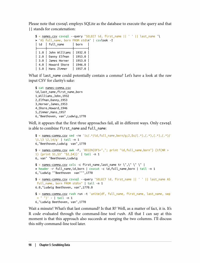
Please note that csvsql employs SQLite as the database to execute the query and that|| stands for concatenation:

$ < names.csv csvsql --query "SELECT id, first_name || ' ' || last_name "\> "AS full_name, born FROM stdin" | csvlook -I│ id │ full_name │ born │├─────┼───────────────┼────────┤│ 1.0 │ John Williams │ 1932.0 ││ 2.0 │ Danny Elfman │ 1953.0 ││ 3.0 │ James Horner │ 1953.0 ││ 4.0 │ Howard Shore │ 1946.0 ││ 5.0 │ Hans Zimmer │ 1957.0 │

What if last_name could potentially contain a comma? Let’s have a look at the rawinput CSV for clarity’s sake:

$ cat names-comma.csvid,last_name,first_name,born1,Williams,John,19322,Elfman,Danny,19533,Horner,James,19534,Shore,Howard,19465,Zimmer,Hans,19576,"Beethoven, van",Ludwig,1770

Well, it appears that the first three approaches fail, all in different ways. Only csvsqlis able to combine first_name and full_name:

$ < names-comma.csv sed -re '1s/.*/id,full_name,born/g;2,$s/(.*),(.*),(.*),(.*)/\1,\3 \2,\4/g' | tail -n 16,"Beethoven,Ludwig van",1770

$ < names-comma.csv awk -F, 'BEGIN{OFS=","; print "id,full_name,born"} {if(NR >1) {print $1,$3" "$2,$4}}' | tail -n 16, van" "Beethoven,Ludwig

$ < names-comma.csv cols -c first_name,last_name tr \",\" \" \" |> header -r full_name,id,born | csvcut -c id,full_name,born | tail -n 16,"Ludwig ""Beethoven van""",1770

$ < names-comma.csv csvsql --query "SELECT id, first_name || ' ' || last_name AS full_name, born FROM stdin" | tail -n 16.0,"Ludwig Beethoven, van",1770.0

$ < names-comma.csv rush run -t 'unite(df, full_name, first_name, last_name, sep = " ")' - | tail -n 16,"Ludwig Beethoven, van",1770

Wait a minute! What’s that last command? Is that R? Well, as a matter of fact, it is. It’sR code evaluated through the command-line tool rush. All that I can say at thismoment is that this approach also succeeds at merging the two columns. I’ll discussthis nifty command-line tool later.

98 | Chapter 5: Scrubbing Data

17 Mike Parker, Richard M. Stallman, and David MacKenzie, tee – Read from Standard Input and Write to Stan‐dard Output and Files, version 8.30, 2019, https://www.gnu.org/software/coreutils.

Combining Multiple CSV FilesIf you start out with multiple CSV files, it’s often a good idea to combine them. Whenthe CSV files have the same columns, you can concatenate them horizontally. Whenthe CSV files have different column names but are still related, you can often jointhem.

Concatenate horizontally

Let’s say you have three CSV files that you want to put side by side. We use tee17 tosave the result of csvcut in the middle of the pipeline:

$ < tips.csv csvcut -c bill,tip | tee bills.csv | head -n 3 | csvlook│ bill │ tip │├───────┼──────┤│ 16.99 │ 1.01 ││ 10.34 │ 1.66 │ $ < tips.csv csvcut -c day,time | tee datetime.csv |> head -n 3 | csvlook -I│ day │ time │├─────┼────────┤│ Sun │ Dinner ││ Sun │ Dinner │ $ < tips.csv csvcut -c sex,smoker,size | tee customers.csv |> head -n 3 | csvlook│ sex │ smoker │ size │├────────┼────────┼──────┤│ Female │ False │ 2 ││ Male │ False │ 3 │

Assuming that the rows line up, you can paste the files together:

$ paste -d, {bills,customers,datetime}.csv | head -n 3 | csvlook -I│ bill │ tip │ sex │ smoker │ size │ day │ time │├───────┼──────┼────────┼────────┼──────┼─────┼────────┤│ 16.99 │ 1.01 │ Female │ No │ 2 │ Sun │ Dinner ││ 10.34 │ 1.66 │ Male │ No │ 3 │ Sun │ Dinner │

Here the command-line argument -d instructs paste to use a comma as thedelimiter.

CSV | 99

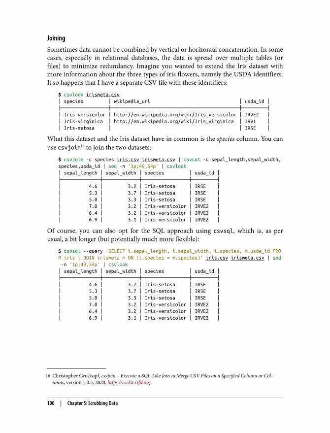
18 Christopher Groskopf, csvjoin – Execute a SQL-Like Join to Merge CSV Files on a Specified Column or Col‐umns, version 1.0.5, 2020, https://csvkit.rtfd.org.

JoiningSometimes data cannot be combined by vertical or horizontal concatenation. In somecases, especially in relational databases, the data is spread over multiple tables (orfiles) to minimize redundancy. Imagine you wanted to extend the Iris dataset withmore information about the three types of iris flowers, namely the USDA identifiers.It so happens that I have a separate CSV file with these identifiers:

$ csvlook irismeta.csv│ species │ wikipedia_url │ usda_id │├─────────────────┼──────────────────────────────────────────────┼─────────┤│ Iris-versicolor │ http://en.wikipedia.org/wiki/Iris_versicolor │ IRVE2 ││ Iris-virginica │ http://en.wikipedia.org/wiki/Iris_virginica │ IRVI ││ Iris-setosa │ │ IRSE │

What this dataset and the Iris dataset have in common is the species column. You canuse csvjoin18 to join the two datasets:

$ csvjoin -c species iris.csv irismeta.csv | csvcut -c sepal_length,sepal_width,species,usda_id | sed -n '1p;49,54p' | csvlook│ sepal_length │ sepal_width │ species │ usda_id │├──────────────┼─────────────┼─────────────────┼─────────┤│ 4.6 │ 3.2 │ Iris-setosa │ IRSE ││ 5.3 │ 3.7 │ Iris-setosa │ IRSE ││ 5.0 │ 3.3 │ Iris-setosa │ IRSE ││ 7.0 │ 3.2 │ Iris-versicolor │ IRVE2 ││ 6.4 │ 3.2 │ Iris-versicolor │ IRVE2 ││ 6.9 │ 3.1 │ Iris-versicolor │ IRVE2 │

Of course, you can also opt for the SQL approach using csvsql, which is, as perusual, a bit longer (but potentially much more flexible):

$ csvsql --query 'SELECT i.sepal_length, i.sepal_width, i.species, m.usda_id FROM iris i JOIN irismeta m ON (i.species = m.species)' iris.csv irismeta.csv | sed -n '1p;49,54p' | csvlook│ sepal_length │ sepal_width │ species │ usda_id │├──────────────┼─────────────┼─────────────────┼─────────┤│ 4.6 │ 3.2 │ Iris-setosa │ IRSE ││ 5.3 │ 3.7 │ Iris-setosa │ IRSE ││ 5.0 │ 3.3 │ Iris-setosa │ IRSE ││ 7.0 │ 3.2 │ Iris-versicolor │ IRVE2 ││ 6.4 │ 3.2 │ Iris-versicolor │ IRVE2 ││ 6.9 │ 3.1 │ Iris-versicolor │ IRVE2 │

100 | Chapter 5: Scrubbing Data

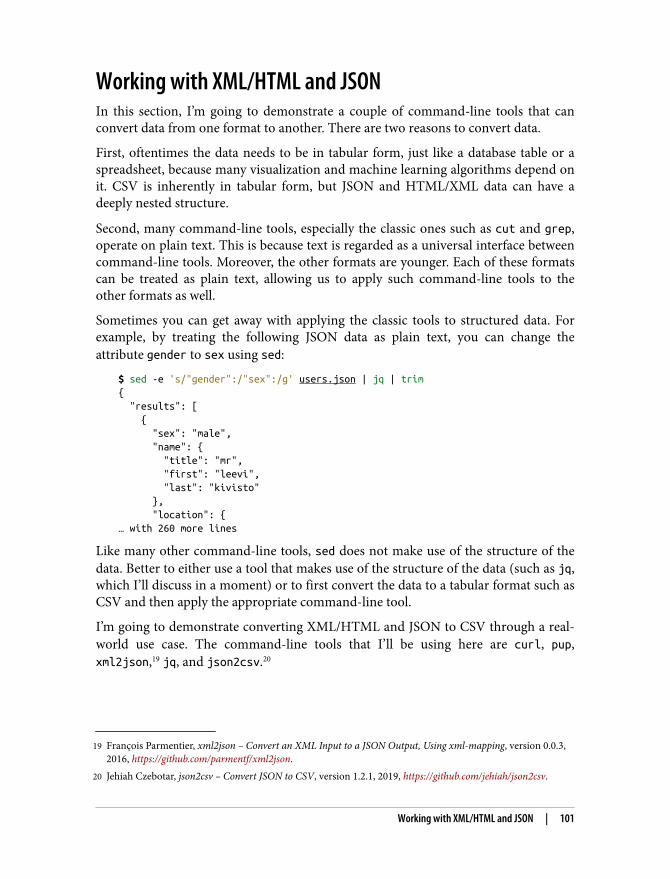
19 François Parmentier, xml2json – Convert an XML Input to a JSON Output, Using xml-mapping, version 0.0.3,2016, https://github.com/parmentf/xml2json.

20 Jehiah Czebotar, json2csv – Convert JSON to CSV, version 1.2.1, 2019, https://github.com/jehiah/json2csv.

Working with XML/HTML and JSONIn this section, I’m going to demonstrate a couple of command-line tools that canconvert data from one format to another. There are two reasons to convert data.

First, oftentimes the data needs to be in tabular form, just like a database table or aspreadsheet, because many visualization and machine learning algorithms depend onit. CSV is inherently in tabular form, but JSON and HTML/XML data can have adeeply nested structure.

Second, many command-line tools, especially the classic ones such as cut and grep,operate on plain text. This is because text is regarded as a universal interface betweencommand-line tools. Moreover, the other formats are younger. Each of these formatscan be treated as plain text, allowing us to apply such command-line tools to theother formats as well.

Sometimes you can get away with applying the classic tools to structured data. Forexample, by treating the following JSON data as plain text, you can change theattribute gender to sex using sed:

$ sed -e 's/"gender":/"sex":/g' users.json | jq | trim{ "results": [ { "sex": "male", "name": { "title": "mr", "first": "leevi", "last": "kivisto" }, "location": {… with 260 more lines

Like many other command-line tools, sed does not make use of the structure of thedata. Better to either use a tool that makes use of the structure of the data (such as jq,which I’ll discuss in a moment) or to first convert the data to a tabular format such asCSV and then apply the appropriate command-line tool.

I’m going to demonstrate converting XML/HTML and JSON to CSV through a real-world use case. The command-line tools that I’ll be using here are curl, pup,xml2json,19 jq, and json2csv.20

Working with XML/HTML and JSON | 101

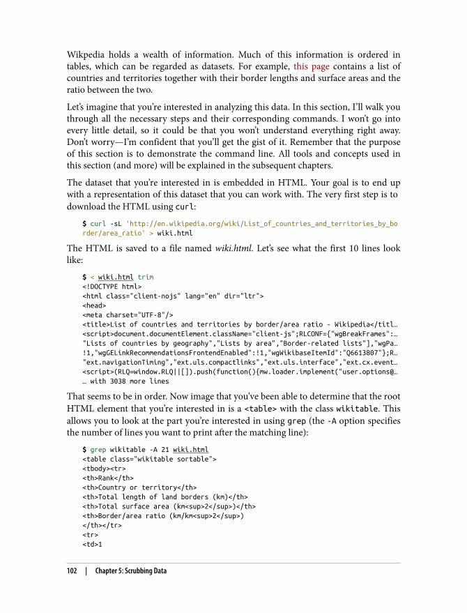
Wikpedia holds a wealth of information. Much of this information is ordered intables, which can be regarded as datasets. For example, this page contains a list ofcountries and territories together with their border lengths and surface areas and theratio between the two.

Let’s imagine that you’re interested in analyzing this data. In this section, I’ll walk youthrough all the necessary steps and their corresponding commands. I won’t go intoevery little detail, so it could be that you won’t understand everything right away.Don’t worry—I’m confident that you’ll get the gist of it. Remember that the purposeof this section is to demonstrate the command line. All tools and concepts used inthis section (and more) will be explained in the subsequent chapters.

The dataset that you’re interested in is embedded in HTML. Your goal is to end upwith a representation of this dataset that you can work with. The very first step is to download the HTML using curl:

$ curl -sL 'http://en.wikipedia.org/wiki/List_of_countries_and_territories_by_border/area_ratio' > wiki.html

The HTML is saved to a file named wiki.html. Let’s see what the first 10 lines looklike:

$ < wiki.html trim<!DOCTYPE html><html class="client-nojs" lang="en" dir="ltr"><head><meta charset="UTF-8"/><title>List of countries and territories by border/area ratio - Wikipedia</titl…<script>document.documentElement.className="client-js";RLCONF={"wgBreakFrames":…"Lists of countries by geography","Lists by area","Border-related lists"],"wgPa…!1,"wgGELinkRecommendationsFrontendEnabled":!1,"wgWikibaseItemId":"Q6613807"};R…"ext.navigationTiming","ext.uls.compactlinks","ext.uls.interface","ext.cx.event…<script>(RLQ=window.RLQ||[]).push(function(){mw.loader.implement("user.options@…… with 3038 more lines

That seems to be in order. Now image that you’ve been able to determine that the rootHTML element that you’re interested in is a <table> with the class wikitable. Thisallows you to look at the part you’re interested in using grep (the -A option specifiesthe number of lines you want to print after the matching line):

$ grep wikitable -A 21 wiki.html<table class="wikitable sortable"><tbody><tr><th>Rank</th><th>Country or territory</th><th>Total length of land borders (km)</th><th>Total surface area (km²)</th><th>Border/area ratio (km/km²)</th></tr><tr><td>1

102 | Chapter 5: Scrubbing Data

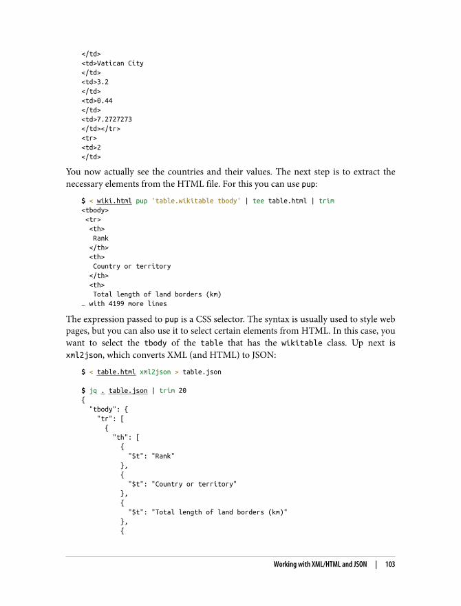
</td><td>Vatican City</td><td>3.2</td><td>0.44</td><td>7.2727273</td></tr><tr><td>2</td>

You now actually see the countries and their values. The next step is to extract thenecessary elements from the HTML file. For this you can use pup:

$ < wiki.html pup 'table.wikitable tbody' | tee table.html | trim<tbody> <tr> <th> Rank </th> <th> Country or territory </th> <th> Total length of land borders (km)… with 4199 more lines

The expression passed to pup is a CSS selector. The syntax is usually used to style webpages, but you can also use it to select certain elements from HTML. In this case, youwant to select the tbody of the table that has the wikitable class. Up next isxml2json, which converts XML (and HTML) to JSON:

$ < table.html xml2json > table.json $ jq . table.json | trim 20{ "tbody": { "tr": [ { "th": [ { "$t": "Rank" }, { "$t": "Country or territory" }, { "$t": "Total length of land borders (km)" }, {

Working with XML/HTML and JSON | 103

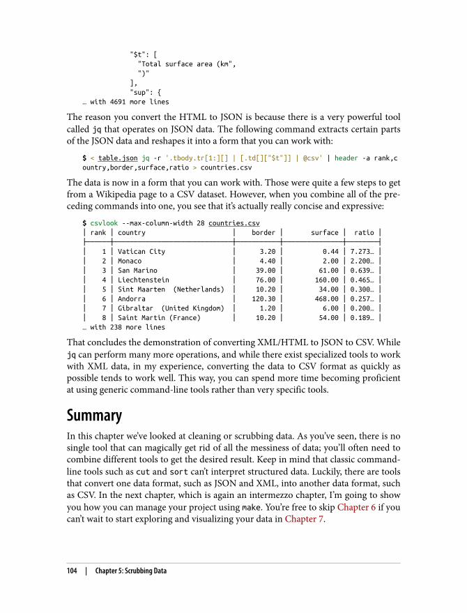
"$t": [ "Total surface area (km", ")" ], "sup": {… with 4691 more lines

The reason you convert the HTML to JSON is because there is a very powerful toolcalled jq that operates on JSON data. The following command extracts certain partsof the JSON data and reshapes it into a form that you can work with:

$ < table.json jq -r '.tbody.tr[1:][] | [.td[]["$t"]] | @csv' | header -a rank,country,border,surface,ratio > countries.csv

The data is now in a form that you can work with. Those were quite a few steps to getfrom a Wikipedia page to a CSV dataset. However, when you combine all of the pre‐ceding commands into one, you see that it’s actually really concise and expressive:

$ csvlook --max-column-width 28 countries.csv│ rank │ country │ border │ surface │ ratio │├──────┼──────────────────────────────┼───────────┼───────────────┼────────┤│ 1 │ Vatican City │ 3.20 │ 0.44 │ 7.273… ││ 2 │ Monaco │ 4.40 │ 2.00 │ 2.200… ││ 3 │ San Marino │ 39.00 │ 61.00 │ 0.639… ││ 4 │ Liechtenstein │ 76.00 │ 160.00 │ 0.465… ││ 5 │ Sint Maarten (Netherlands) │ 10.20 │ 34.00 │ 0.300… ││ 6 │ Andorra │ 120.30 │ 468.00 │ 0.257… ││ 7 │ Gibraltar (United Kingdom) │ 1.20 │ 6.00 │ 0.200… ││ 8 │ Saint Martin (France) │ 10.20 │ 54.00 │ 0.189… │… with 238 more lines

That concludes the demonstration of converting XML/HTML to JSON to CSV. Whilejq can perform many more operations, and while there exist specialized tools to workwith XML data, in my experience, converting the data to CSV format as quickly aspossible tends to work well. This way, you can spend more time becoming proficientat using generic command-line tools rather than very specific tools.

SummaryIn this chapter we’ve looked at cleaning or scrubbing data. As you’ve seen, there is nosingle tool that can magically get rid of all the messiness of data; you’ll often need tocombine different tools to get the desired result. Keep in mind that classic command-line tools such as cut and sort can’t interpret structured data. Luckily, there are toolsthat convert one data format, such as JSON and XML, into another data format, suchas CSV. In the next chapter, which is again an intermezzo chapter, I’m going to showyou how you can manage your project using make. You’re free to skip Chapter 6 if youcan’t wait to start exploring and visualizing your data in Chapter 7.

104 | Chapter 5: Scrubbing Data

For Further Exploration• I wish I could’ve explained more about awk. It’s such a powerful tool and pro‐

gramming language. I highly recommend that you take the time to learn it. Twogood resources for that are the book sed & awk by Dale Doherty and ArnoldRobbins (O’Reilly) and the online GNU Awk User’s Guide.

• In this chapter I have used regular expressions in a couple of places. A tutorialabout them is unfortunately beyond the scope of this book. Because regularexpressions can be used in many different tools, I recommend that you learnabout them. A good book for this is Regular Expressions Cookbook by Jan Goy‐vaerts and Steven Levithan (O’Reilly).

For Further Exploration | 105

CHAPTER 6

Project Management with Make

I hope that by now you have come to appreciate that the command line is a very con‐venient environment for working with data. You may have noticed that, as a conse‐quence of working with the command line, we:

• Invoke many different commands• Work from various directories• Develop our own command-line tools• Obtain and generate many (intermediate) files

Since this is an exploratory process, our workflow tends to be rather chaotic, whichmakes it difficult to keep track of what we’ve done. It’s important that our steps can bereproduced, both by us and by others. When you continue with a project from sometime ago, chances are that you have forgotten which commands you ran, from whichdirectory, on which files, with which parameters, and in which order. Imagine thechallenges of sharing your project with a collaborator.

You can recover some commands by digging through the output of the history com‐mand, but this is, of course, not a reliable approach. A somewhat better approachwould be to save your commands to a shell script. At least this allows you and yourcollaborators to reproduce the project. A shell script is, however, also suboptimal, forseveral reasons:

• It is difficult to read and to maintain.• Dependencies between steps are unclear.• Every step gets executed every time, which is inefficient and is also sometimes

undesirable.

107

1 Stuart I. Feldman, make – A Program for Maintaining Computer Programs, version 4.3, 2020, https://www.gnu.org/software/make.

2 Factual, drake – Data Workflow Tool, like a “Make for Data,” version 1.0.3, 2016, https://github.com/Factual/drake.

This is where make really shines. make1 is a command-line tool that allows you to:

• Formalize your data workflow steps in terms of input and output dependencies• Run specific steps of your workflow• Use inline code• Store and retrieve data from external sources

In the first edition, this chapter used drake2 instead of make. drakewas supposed to be a successor to make with additional features forworking with data. Unfortunately, drake was abandoned by its cre‐ators in 2016 with too many unresolved bugs. That’s why I’ve deci‐ded to use make instead.

An important and related topic is version control, which allows you to track changesto your project, back up your project to a server, collaborate with others, and retrieveearlier versions of your project when things go wrong. A popular command-line tool for doing version control is git. It’s often used in combination with GitHub, anonline service for distributed version control. Many open source projects, includingthis book, are hosted on GitHub. The topic of version control is beyond the scope ofthis book, but I highly recommend that you look into this, especially once you startcollaborating with others. At the end of this chapter I recommend a few resources forlearning more.

OverviewManaging your data workflow with make is the main topic of this chapter. As such,you’ll learn about:

• Defining your workflow with a Makefile• Thinking about your workflow in terms of input and output dependencies• Running tasks and building targets

This chapter starts with the following files:

$ cd /data/ch06

108 | Chapter 6: Project Management with Make

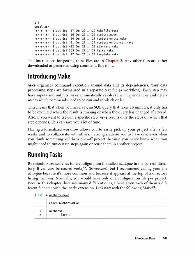
$ ltotal 28K-rw-r--r-- 1 dst dst 37 Jun 29 14:29 Makefile.test-rw-r--r-- 1 dst dst 16 Jun 29 14:29 numbers.make-rw-r--r-- 1 dst dst 26 Jun 29 14:29 numbers-write.make-rw-r--r-- 1 dst dst 21 Jun 29 14:29 numbers-write-var.make-rw-r--r-- 1 dst dst 432 Jun 29 14:29 starwars.make-rw-r--r-- 1 dst dst 263 Jun 29 14:29 tasks.make-rw-r--r-- 1 dst dst 27 Jun 29 14:29 template.make

The instructions for getting these files are in Chapter 2. Any other files are eitherdownloaded or generated using command-line tools.

Introducing Makemake organizes command execution around data and its dependencies. Your dataprocessing steps are formalized in a separate text file (a workflow). Each step mayhave inputs and outputs. make automatically resolves their dependencies and deter‐mines which commands need to be run and in which order.

This means that when you have, say, an SQL query that takes 10 minutes, it only hasto be executed when the result is missing or when the query has changed afterward.Also, if you want to (re)run a specific step, make reruns only the steps on which thatstep depends. This can save you a lot of time.

Having a formalized workflow allows you to easily pick up your project after a fewweeks and to collaborate with others. I strongly advise you to have one, even whenyou think something will be a one-off project, because you never know when youmight need to run certain steps again or reuse them in another project.

Running TasksBy default, make searches for a configuration file called Makefile in the current direc‐tory. It can also be named makefile (lowercase), but I recommend calling your fileMakefile because it’s more common and because it appears at the top of a directorylisting that way. Normally, you would have only one configuration file per project.Because this chapter discusses many different ones, I have given each of them a dif‐ferent filename with the .make extension. Let’s start with the following Makefile:

$ bat -A numbers.make───────┬──────────────────────────────────────────────────────────────────────── │ File: numbers.make───────┼──────────────────────────────────────────────────────────────────────── 1 │ numbers:␊ 2 │ ├──────┤seq·7␊───────┴────────────────────────────────────────────────────────────────────────

Introducing Make | 109

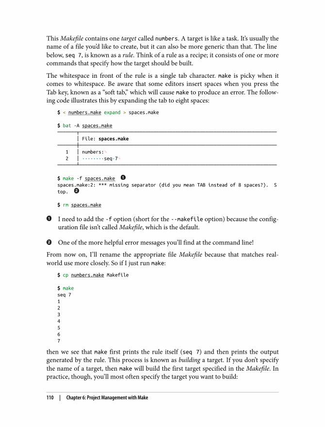
This Makefile contains one target called numbers. A target is like a task. It’s usually thename of a file you’d like to create, but it can also be more generic than that. The line below, seq 7, is known as a rule. Think of a rule as a recipe; it consists of one or morecommands that specify how the target should be built.

The whitespace in front of the rule is a single tab character. make is picky when itcomes to whitespace. Be aware that some editors insert spaces when you press theTab key, known as a “soft tab,” which will cause make to produce an error. The follow‐ing code illustrates this by expanding the tab to eight spaces:

$ < numbers.make expand > spaces.make $ bat -A spaces.make───────┬──────────────────────────────────────────────────────────────────────── │ File: spaces.make───────┼──────────────────────────────────────────────────────────────────────── 1 │ numbers:␊ 2 │ ········seq·7␊───────┴──────────────────────────────────────────────────────────────────────── $ make -f spaces.make spaces.make:2: *** missing separator (did you mean TAB instead of 8 spaces?). Stop. $ rm spaces.make

I need to add the -f option (short for the --makefile option) because the config‐uration file isn’t called Makefile, which is the default.

One of the more helpful error messages you’ll find at the command line!

From now on, I’ll rename the appropriate file Makefile because that matches real-world use more closely. So if I just run make:

$ cp numbers.make Makefile $ makeseq 71234567

then we see that make first prints the rule itself (seq 7) and then prints the outputgenerated by the rule. This process is known as building a target. If you don’t specifythe name of a target, then make will build the first target specified in the Makefile. Inpractice, though, you’ll most often specify the target you want to build:

110 | Chapter 6: Project Management with Make

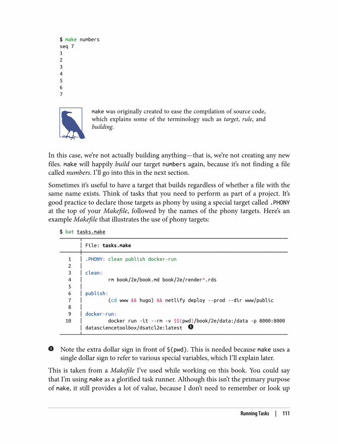
$ make numbersseq 71234567

make was originally created to ease the compilation of source code,which explains some of the terminology such as target, rule, andbuilding.

In this case, we’re not actually building anything—that is, we’re not creating any newfiles. make will happily build our target numbers again, because it’s not finding a filecalled numbers. I’ll go into this in the next section.

Sometimes it’s useful to have a target that builds regardless of whether a file with thesame name exists. Think of tasks that you need to perform as part of a project. It’sgood practice to declare those targets as phony by using a special target called .PHONYat the top of your Makefile, followed by the names of the phony targets. Here’s anexample Makefile that illustrates the use of phony targets:

$ bat tasks.make───────┬──────────────────────────────────────────────────────────────────────── │ File: tasks.make───────┼──────────────────────────────────────────────────────────────────────── 1 │ .PHONY: clean publish docker-run 2 │ 3 │ clean: 4 │ rm book/2e/book.md book/2e/render*.rds 5 │ 6 │ publish: 7 │ (cd www && hugo) && netlify deploy --prod --dir www/public 8 │ 9 │ docker-run: 10 │ docker run -it --rm -v $$(pwd)/book/2e/data:/data -p 8000:8000 │ datasciencetoolbox/dsatcl2e:latest ───────┴────────────────────────────────────────────────────────────────────────

Note the extra dollar sign in front of $(pwd). This is needed because make uses asingle dollar sign to refer to various special variables, which I’ll explain later.

This is taken from a Makefile I’ve used while working on this book. You could saythat I’m using make as a glorified task runner. Although this isn’t the primary purposeof make, it still provides a lot of value, because I don’t need to remember or look up

Running Tasks | 111

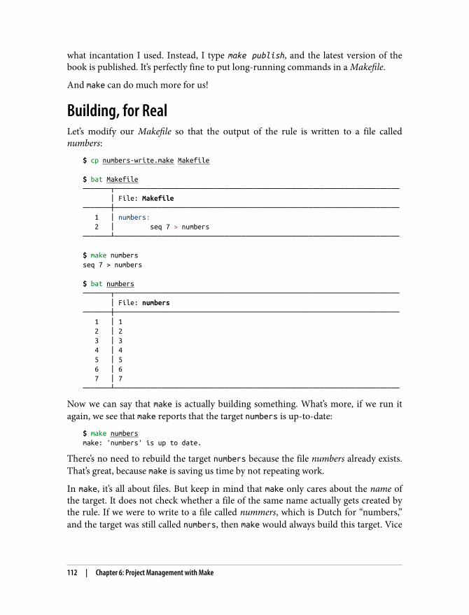
what incantation I used. Instead, I type make publish, and the latest version of thebook is published. It’s perfectly fine to put long-running commands in a Makefile.

And make can do much more for us!

Building, for RealLet’s modify our Makefile so that the output of the rule is written to a file callednumbers:

$ cp numbers-write.make Makefile $ bat Makefile───────┬──────────────────────────────────────────────────────────────────────── │ File: Makefile───────┼──────────────────────────────────────────────────────────────────────── 1 │ numbers: 2 │ seq 7 > numbers───────┴──────────────────────────────────────────────────────────────────────── $ make numbersseq 7 > numbers $ bat numbers───────┬──────────────────────────────────────────────────────────────────────── │ File: numbers───────┼──────────────────────────────────────────────────────────────────────── 1 │ 1 2 │ 2 3 │ 3 4 │ 4 5 │ 5 6 │ 6 7 │ 7───────┴────────────────────────────────────────────────────────────────────────

Now we can say that make is actually building something. What’s more, if we run itagain, we see that make reports that the target numbers is up-to-date:

$ make numbersmake: 'numbers' is up to date.

There’s no need to rebuild the target numbers because the file numbers already exists.That’s great, because make is saving us time by not repeating work.

In make, it’s all about files. But keep in mind that make only cares about the name ofthe target. It does not check whether a file of the same name actually gets created bythe rule. If we were to write to a file called nummers, which is Dutch for “numbers,”and the target was still called numbers, then make would always build this target. Vice

112 | Chapter 6: Project Management with Make

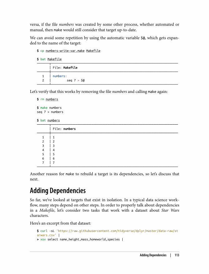
versa, if the file numbers was created by some other process, whether automated ormanual, then make would still consider that target up-to-date.

We can avoid some repetition by using the automatic variable $@, which gets expan‐ded to the name of the target:

$ cp numbers-write-var.make Makefile $ bat Makefile───────┬──────────────────────────────────────────────────────────────────────── │ File: Makefile───────┼──────────────────────────────────────────────────────────────────────── 1 │ numbers: 2 │ seq 7 > $@───────┴────────────────────────────────────────────────────────────────────────

Let’s verify that this works by removing the file numbers and calling make again:

$ rm numbers $ make numbersseq 7 > numbers $ bat numbers───────┬──────────────────────────────────────────────────────────────────────── │ File: numbers───────┼──────────────────────────────────────────────────────────────────────── 1 │ 1 2 │ 2 3 │ 3 4 │ 4 5 │ 5 6 │ 6 7 │ 7───────┴────────────────────────────────────────────────────────────────────────

Another reason for make to rebuild a target is its dependencies, so let’s discuss thatnext.

Adding DependenciesSo far, we’ve looked at targets that exist in isolation. In a typical data science work‐flow, many steps depend on other steps. In order to properly talk about dependenciesin a Makefile, let’s consider two tasks that work with a dataset about Star Warscharacters.

Here’s an excerpt from that dataset:

$ curl -sL 'https://raw.githubusercontent.com/tidyverse/dplyr/master/data-raw/starwars.csv' |> xsv select name,height,mass,homeworld,species |

Adding Dependencies | 113

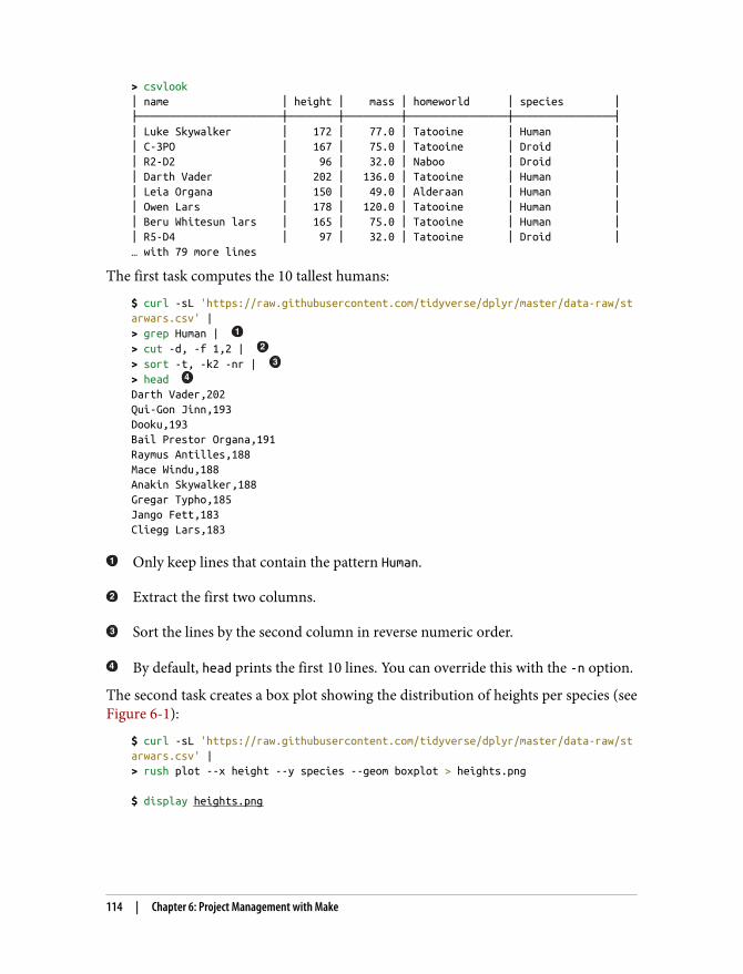
> csvlook│ name │ height │ mass │ homeworld │ species │├───────────────────────┼────────┼─────────┼────────────────┼────────────────┤│ Luke Skywalker │ 172 │ 77.0 │ Tatooine │ Human ││ C-3PO │ 167 │ 75.0 │ Tatooine │ Droid ││ R2-D2 │ 96 │ 32.0 │ Naboo │ Droid ││ Darth Vader │ 202 │ 136.0 │ Tatooine │ Human ││ Leia Organa │ 150 │ 49.0 │ Alderaan │ Human ││ Owen Lars │ 178 │ 120.0 │ Tatooine │ Human ││ Beru Whitesun lars │ 165 │ 75.0 │ Tatooine │ Human ││ R5-D4 │ 97 │ 32.0 │ Tatooine │ Droid │… with 79 more lines

The first task computes the 10 tallest humans:

$ curl -sL 'https://raw.githubusercontent.com/tidyverse/dplyr/master/data-raw/starwars.csv' |> grep Human | > cut -d, -f 1,2 | > sort -t, -k2 -nr | > head Darth Vader,202Qui-Gon Jinn,193Dooku,193Bail Prestor Organa,191Raymus Antilles,188Mace Windu,188Anakin Skywalker,188Gregar Typho,185Jango Fett,183Cliegg Lars,183

Only keep lines that contain the pattern Human.

Extract the first two columns.

Sort the lines by the second column in reverse numeric order.

By default, head prints the first 10 lines. You can override this with the -n option.

The second task creates a box plot showing the distribution of heights per species (seeFigure 6-1):

$ curl -sL 'https://raw.githubusercontent.com/tidyverse/dplyr/master/data-raw/starwars.csv' |> rush plot --x height --y species --geom boxplot > heights.png $ display heights.png

114 | Chapter 6: Project Management with Make

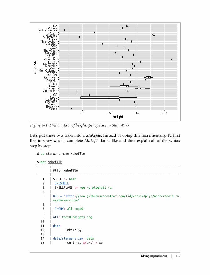
Figure 6-1. Distribution of heights per species in Star Wars

Let’s put these two tasks into a Makefile. Instead of doing this incrementally, I’d firstlike to show what a complete Makefile looks like and then explain all of the syntaxstep by step:

$ cp starwars.make Makefile $ bat Makefile───────┬──────────────────────────────────────────────────────────────────────── │ File: Makefile───────┼──────────────────────────────────────────────────────────────────────── 1 │ SHELL := bash 2 │ .ONESHELL: 3 │ .SHELLFLAGS := -eu -o pipefail -c 4 │ 5 │ URL = "https://raw.githubusercontent.com/tidyverse/dplyr/master/data-ra │ w/starwars.csv" 6 │ 7 │ .PHONY: all top10 8 │ 9 │ all: top10 heights.png 10 │ 11 │ data: 12 │ mkdir $@ 13 │ 14 │ data/starwars.csv: data 15 │ curl -sL $(URL) > $@

Adding Dependencies | 115

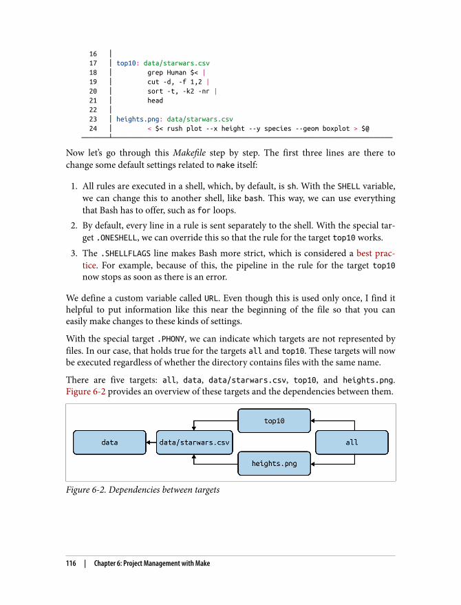
16 │ 17 │ top10: data/starwars.csv 18 │ grep Human $< | 19 │ cut -d, -f 1,2 | 20 │ sort -t, -k2 -nr | 21 │ head 22 │ 23 │ heights.png: data/starwars.csv 24 │ < $< rush plot --x height --y species --geom boxplot > $@───────┴────────────────────────────────────────────────────────────────────────

Now let’s go through this Makefile step by step. The first three lines are there tochange some default settings related to make itself:

1. All rules are executed in a shell, which, by default, is sh. With the SHELL variable,we can change this to another shell, like bash. This way, we can use everythingthat Bash has to offer, such as for loops.

2. By default, every line in a rule is sent separately to the shell. With the special tar‐get .ONESHELL, we can override this so that the rule for the target top10 works.

3. The .SHELLFLAGS line makes Bash more strict, which is considered a best prac‐tice. For example, because of this, the pipeline in the rule for the target top10now stops as soon as there is an error.

We define a custom variable called URL. Even though this is used only once, I find ithelpful to put information like this near the beginning of the file so that you caneasily make changes to these kinds of settings.

With the special target .PHONY, we can indicate which targets are not represented byfiles. In our case, that holds true for the targets all and top10. These targets will nowbe executed regardless of whether the directory contains files with the same name.

There are five targets: all, data, data/starwars.csv, top10, and heights.png.Figure 6-2 provides an overview of these targets and the dependencies between them.

Figure 6-2. Dependencies between targets

116 | Chapter 6: Project Management with Make

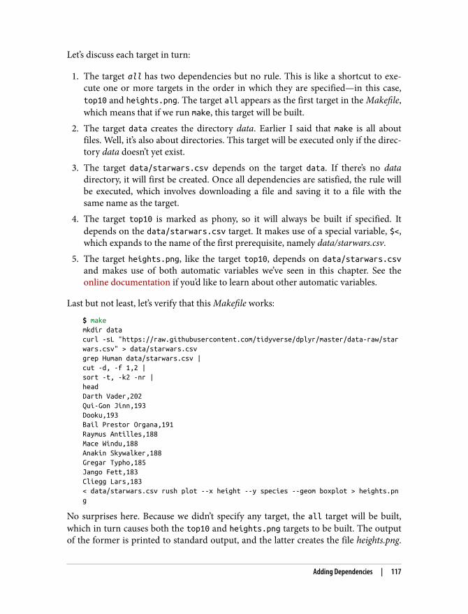
Let’s discuss each target in turn:

1. The target all has two dependencies but no rule. This is like a shortcut to exe‐cute one or more targets in the order in which they are specified—in this case,top10 and heights.png. The target all appears as the first target in the Makefile,which means that if we run make, this target will be built.

2. The target data creates the directory data. Earlier I said that make is all aboutfiles. Well, it’s also about directories. This target will be executed only if the direc‐tory data doesn’t yet exist.

3. The target data/starwars.csv depends on the target data. If there’s no datadirectory, it will first be created. Once all dependencies are satisfied, the rule willbe executed, which involves downloading a file and saving it to a file with thesame name as the target.

4. The target top10 is marked as phony, so it will always be built if specified. Itdepends on the data/starwars.csv target. It makes use of a special variable, $<,which expands to the name of the first prerequisite, namely data/starwars.csv.

5. The target heights.png, like the target top10, depends on data/starwars.csvand makes use of both automatic variables we’ve seen in this chapter. See theonline documentation if you’d like to learn about other automatic variables.

Last but not least, let’s verify that this Makefile works:

$ makemkdir datacurl -sL "https://raw.githubusercontent.com/tidyverse/dplyr/master/data-raw/starwars.csv" > data/starwars.csvgrep Human data/starwars.csv |cut -d, -f 1,2 |sort -t, -k2 -nr |headDarth Vader,202Qui-Gon Jinn,193Dooku,193Bail Prestor Organa,191Raymus Antilles,188Mace Windu,188Anakin Skywalker,188Gregar Typho,185Jango Fett,183Cliegg Lars,183< data/starwars.csv rush plot --x height --y species --geom boxplot > heights.png

No surprises here. Because we didn’t specify any target, the all target will be built,which in turn causes both the top10 and heights.png targets to be built. The outputof the former is printed to standard output, and the latter creates the file heights.png.

Adding Dependencies | 117

The data directory is created only once, just like the CSV file is downloaded onlyonce.

There’s nothing more fun than just playing with your data and forgetting everythingelse. But you have to trust me when I say that it’s worthwhile to keep a record of whatyou have done using a Makefile. Not only will it make your life easier (pun intended),but you will also start thinking about your data workflow in terms of steps. Just aswith your own command-line toolbox, which you expand over time, the same holdsfor make workflows. The more steps you have defined, the easier it gets to keep doingit, because very often you can reuse certain steps. I hope that you will get used tomake, and that it will make your life easier.

SummaryOne of the beauties of the command line is that it allows you to play with your data.You can easily execute different commands and process different datafiles. It is a veryinteractive and iterative process. After a while, it is easy to forget which steps youhave taken to get the desired result. It’s therefore very important to document yoursteps every once in a while. This way, if you or one of your colleagues picks up yourproject after some time, the same result can be produced again by executing the samesteps.

In this chapter I’ve shown you that just putting every command in one Bash script issuboptimal. Instead, I propose that you use make as a command-line tool to manageyour data workflow. The next chapter covers the third step of the OSEMN model fordata science: exploring data.

For Further Exploration• The book Managing Projects with GNU Make by Robert Mecklenburg (O’Reilly)

and the online GNU Make Manual provide a comprehensive and advanced over‐view of make.

• There are plenty of other workflow managers besides make. Although they differin syntax and features, they all use concepts such as targets, rules, and dependen‐cies. Examples include Luigi, Apache Airflow, and Nextflow.

• To learn more about version control, and about git and GitHub in particular, Irecommend the book Pro Git by Scott Chacon and Ben Straub (Apress); it’s avail‐able for free. The online GitHub documentation is also a great starting point.

118 | Chapter 6: Project Management with Make

CHAPTER 7

Exploring Data

After all that hard work (unless you already had clean data lying around), it’s time forsome fun. Now that you have obtained and scrubbed your data, you can continuewith the third step of the OSEMN model, which is to explore your data.

Exploring is the step where you familiarize yourself with the data. Being familiar withthe data is essential when you want to extract any value from it. For example, know‐ing what kind of features the data has means you know which features are worth fur‐ther exploration and which ones you can use to answer any questions that you have.

Exploring your data can be done from three perspectives. The first perspective is toinspect the data and its properties. Here, you want to find out things like what the rawdata looks like, how many data points the dataset has, and which features the datasethas.

The second is to compute descriptive statistics. This perspective is useful for learningmore about the individual features. The output is often brief and textual and cantherefore be printed on the command line.

The third perspective is to create visualizations of the data. From this perspective youcan gain insight into how multiple features interact. I’ll discuss a way of creating visu‐alizations that can be printed on the command line. However, visualizations are bestsuited for display on a GUI. An advantage of data visualizations over descriptive sta‐tistics is that the former are more flexible and can convey much more information.

119

OverviewIn this chapter, you’ll learn how to:

• Inspect the data and its properties• Compute descriptive statistics• Create data visualizations inside and outside the command line

This chapter starts with the following files:

$ cd /data/ch07 $ ltotal 104K-rw-r--r-- 1 dst dst 125 Jun 29 14:30 datatypes.csv-rw-r--r-- 1 dst dst 7.8K Jun 29 14:30 tips.csv-rw-r--r-- 1 dst dst 83K Jun 29 14:30 venture.csv-rw-r--r-- 1 dst dst 4.6K Jun 29 14:30 venture-wide.csv

The instructions for getting these files are in Chapter 2. Any other files are eitherdownloaded or generated using command-line tools.

Inspecting Data and Its PropertiesIn this section I’ll demonstrate how to inspect your dataset and its properties.Because the upcoming visualization and modeling techniques expect the data to be ina rectangular shape, I’ll assume that the data is in CSV format. You can use the tech‐niques described in Chapter 5 to convert your data to CSV if necessary.

For simplicity’s sake, I’ll also assume that your data has a header. In the first subsec‐tion, I’ll show you a way to determine whether that’s the case. Once you know youhave a header, you can continue answering the following questions:

• How many data points and features does the dataset have?• What does the raw data look like?• What kind of features does the dataset have?• Can some of these features be treated as categorical?

Header or Not, Here I ComeYou can check whether your file has a header by printing the first few lines usinghead:

$ head -n 5 venture.csvFREQ,TIME_FORMAT,TIME_PERIOD,EXPEND,UNIT,GEO,OBS_STATUS,OBS_VALUE,FREQ_DESC,TIME

120 | Chapter 7: Exploring Data

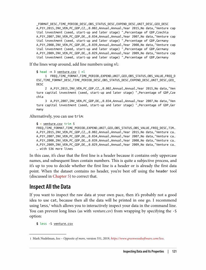
1 Mark Nudelman, less – Opposite of more, version 551, 2019, https://www.greenwoodsoftware.com/less.

_FORMAT_DESC,TIME_PERIOD_DESC,OBS_STATUS_DESC,EXPEND_DESC,UNIT_DESC,GEO_DESCA,P1Y,2015,INV_VEN,PC_GDP,CZ,,0.002,Annual,Annual,Year 2015,No data,"Venture capital investment (seed, start-up and later stage) ",Percentage of GDP,CzechiaA,P1Y,2007,INV_VEN,PC_GDP,DE,,0.034,Annual,Annual,Year 2007,No data,"Venture capital investment (seed, start-up and later stage) ",Percentage of GDP,GermanyA,P1Y,2008,INV_VEN,PC_GDP,DE,,0.039,Annual,Annual,Year 2008,No data,"Venture capital investment (seed, start-up and later stage) ",Percentage of GDP,GermanyA,P1Y,2009,INV_VEN,PC_GDP,DE,,0.029,Annual,Annual,Year 2009,No data,"Venture capital investment (seed, start-up and later stage) ",Percentage of GDP,Germany

If the lines wrap around, add line numbers using nl:

$ head -n 3 venture.csv | nl 1 FREQ,TIME_FORMAT,TIME_PERIOD,EXPEND,UNIT,GEO,OBS_STATUS,OBS_VALUE,FREQ_DESC,TIME_FORMAT_DESC,TIME_PERIOD_DESC,OBS_STATUS_DESC,EXPEND_DESC,UNIT_DESC,GEO_DESC 2 A,P1Y,2015,INV_VEN,PC_GDP,CZ,,0.002,Annual,Annual,Year 2015,No data,"Venture capital investment (seed, start-up and later stage) ",Percentage of GDP,Czechia 3 A,P1Y,2007,INV_VEN,PC_GDP,DE,,0.034,Annual,Annual,Year 2007,No data,"Venture capital investment (seed, start-up and later stage) ",Percentage of GDP,Germany

Alternatively, you can use trim:

$ < venture.csv trim 5FREQ,TIME_FORMAT,TIME_PERIOD,EXPEND,UNIT,GEO,OBS_STATUS,OBS_VALUE,FREQ_DESC,TIM…A,P1Y,2015,INV_VEN,PC_GDP,CZ,,0.002,Annual,Annual,Year 2015,No data,"Venture ca…A,P1Y,2007,INV_VEN,PC_GDP,DE,,0.034,Annual,Annual,Year 2007,No data,"Venture ca…A,P1Y,2008,INV_VEN,PC_GDP,DE,,0.039,Annual,Annual,Year 2008,No data,"Venture ca…A,P1Y,2009,INV_VEN,PC_GDP,DE,,0.029,Annual,Annual,Year 2009,No data,"Venture ca…… with 536 more lines

In this case, it’s clear that the first line is a header because it contains only uppercasenames, and subsequent lines contain numbers. This is quite a subjective process, andit’s up to you to decide whether the first line is a header or is already the first datapoint. When the dataset contains no header, you’re best off using the header tool(discussed in Chapter 5) to correct that.

Inspect All the DataIf you want to inspect the raw data at your own pace, then it’s probably not a goodidea to use cat, because then all the data will be printed in one go. I recommendusing less,1 which allows you to interactively inspect your data in the command line.You can prevent long lines (as with venture.csv) from wrapping by specifying the -Soption:

$ less -S venture.csv

Inspecting Data and Its Properties | 121

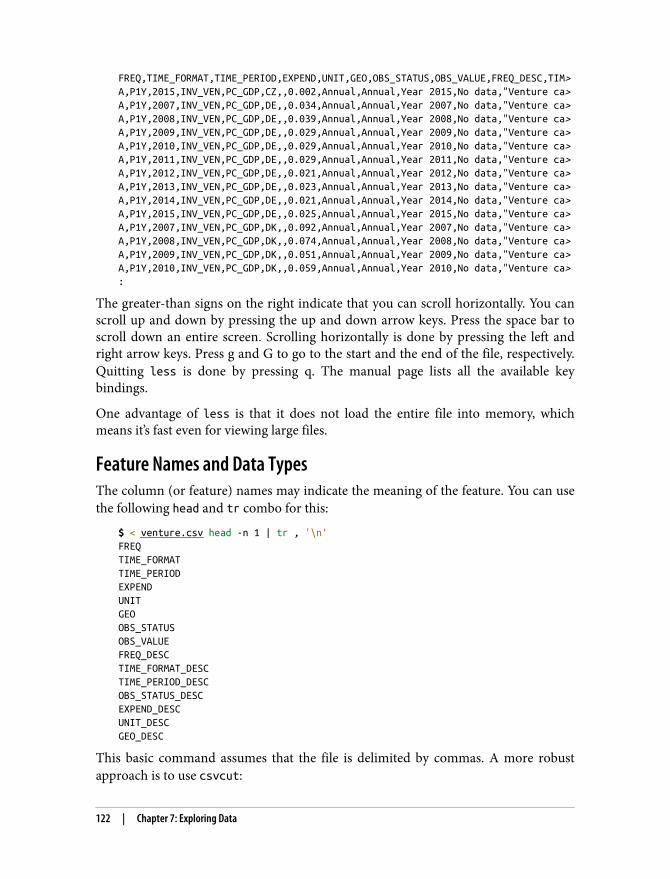
FREQ,TIME_FORMAT,TIME_PERIOD,EXPEND,UNIT,GEO,OBS_STATUS,OBS_VALUE,FREQ_DESC,TIM>A,P1Y,2015,INV_VEN,PC_GDP,CZ,,0.002,Annual,Annual,Year 2015,No data,"Venture ca>A,P1Y,2007,INV_VEN,PC_GDP,DE,,0.034,Annual,Annual,Year 2007,No data,"Venture ca>A,P1Y,2008,INV_VEN,PC_GDP,DE,,0.039,Annual,Annual,Year 2008,No data,"Venture ca>A,P1Y,2009,INV_VEN,PC_GDP,DE,,0.029,Annual,Annual,Year 2009,No data,"Venture ca>A,P1Y,2010,INV_VEN,PC_GDP,DE,,0.029,Annual,Annual,Year 2010,No data,"Venture ca>A,P1Y,2011,INV_VEN,PC_GDP,DE,,0.029,Annual,Annual,Year 2011,No data,"Venture ca>A,P1Y,2012,INV_VEN,PC_GDP,DE,,0.021,Annual,Annual,Year 2012,No data,"Venture ca>A,P1Y,2013,INV_VEN,PC_GDP,DE,,0.023,Annual,Annual,Year 2013,No data,"Venture ca>A,P1Y,2014,INV_VEN,PC_GDP,DE,,0.021,Annual,Annual,Year 2014,No data,"Venture ca>A,P1Y,2015,INV_VEN,PC_GDP,DE,,0.025,Annual,Annual,Year 2015,No data,"Venture ca>A,P1Y,2007,INV_VEN,PC_GDP,DK,,0.092,Annual,Annual,Year 2007,No data,"Venture ca>A,P1Y,2008,INV_VEN,PC_GDP,DK,,0.074,Annual,Annual,Year 2008,No data,"Venture ca>A,P1Y,2009,INV_VEN,PC_GDP,DK,,0.051,Annual,Annual,Year 2009,No data,"Venture ca>A,P1Y,2010,INV_VEN,PC_GDP,DK,,0.059,Annual,Annual,Year 2010,No data,"Venture ca>:

The greater-than signs on the right indicate that you can scroll horizontally. You canscroll up and down by pressing the up and down arrow keys. Press the space bar toscroll down an entire screen. Scrolling horizontally is done by pressing the left andright arrow keys. Press g and G to go to the start and the end of the file, respectively.Quitting less is done by pressing q. The manual page lists all the available keybindings.

One advantage of less is that it does not load the entire file into memory, whichmeans it’s fast even for viewing large files.

Feature Names and Data TypesThe column (or feature) names may indicate the meaning of the feature. You can usethe following head and tr combo for this:

$ < venture.csv head -n 1 | tr , '\n'FREQTIME_FORMATTIME_PERIODEXPENDUNITGEOOBS_STATUSOBS_VALUEFREQ_DESCTIME_FORMAT_DESCTIME_PERIOD_DESCOBS_STATUS_DESCEXPEND_DESCUNIT_DESCGEO_DESC

This basic command assumes that the file is delimited by commas. A more robustapproach is to use csvcut:

122 | Chapter 7: Exploring Data

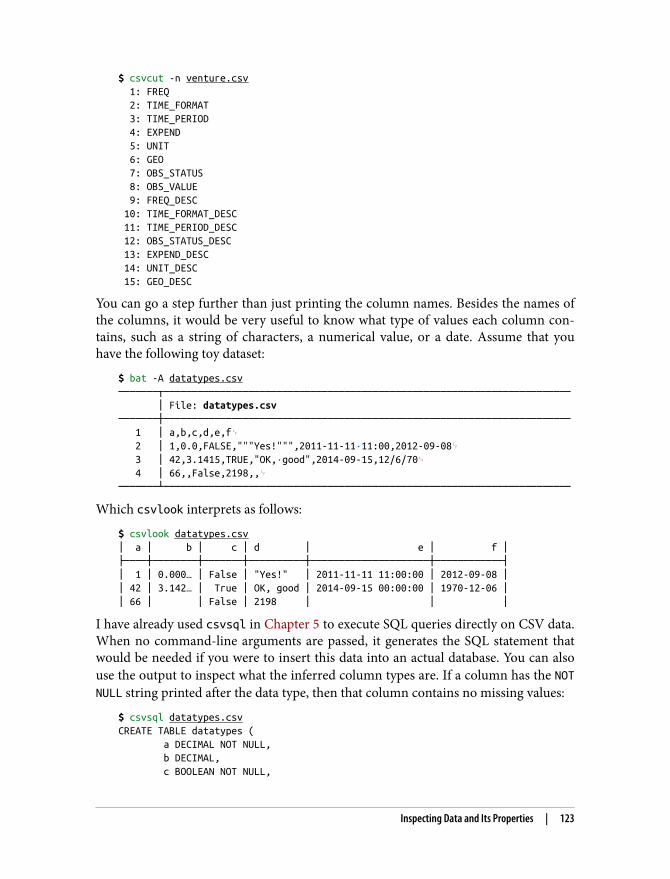
$ csvcut -n venture.csv 1: FREQ 2: TIME_FORMAT 3: TIME_PERIOD 4: EXPEND 5: UNIT 6: GEO 7: OBS_STATUS 8: OBS_VALUE 9: FREQ_DESC 10: TIME_FORMAT_DESC 11: TIME_PERIOD_DESC 12: OBS_STATUS_DESC 13: EXPEND_DESC 14: UNIT_DESC 15: GEO_DESC

You can go a step further than just printing the column names. Besides the names ofthe columns, it would be very useful to know what type of values each column con‐tains, such as a string of characters, a numerical value, or a date. Assume that youhave the following toy dataset:

$ bat -A datatypes.csv───────┬──────────────────────────────────────────────────────────────────────── │ File: datatypes.csv───────┼──────────────────────────────────────────────────────────────────────── 1 │ a,b,c,d,e,f␊ 2 │ 1,0.0,FALSE,"""Yes!""",2011-11-11·11:00,2012-09-08␊ 3 │ 42,3.1415,TRUE,"OK,·good",2014-09-15,12/6/70␊ 4 │ 66,,False,2198,,␊───────┴────────────────────────────────────────────────────────────────────────

Which csvlook interprets as follows:

$ csvlook datatypes.csv│ a │ b │ c │ d │ e │ f │├────┼────────┼───────┼──────────┼─────────────────────┼────────────┤│ 1 │ 0.000… │ False │ "Yes!" │ 2011-11-11 11:00:00 │ 2012-09-08 ││ 42 │ 3.142… │ True │ OK, good │ 2014-09-15 00:00:00 │ 1970-12-06 ││ 66 │ │ False │ 2198 │ │ │

I have already used csvsql in Chapter 5 to execute SQL queries directly on CSV data.When no command-line arguments are passed, it generates the SQL statement thatwould be needed if you were to insert this data into an actual database. You can alsouse the output to inspect what the inferred column types are. If a column has the NOTNULL string printed after the data type, then that column contains no missing values:

$ csvsql datatypes.csvCREATE TABLE datatypes ( a DECIMAL NOT NULL, b DECIMAL, c BOOLEAN NOT NULL,

Inspecting Data and Its Properties | 123

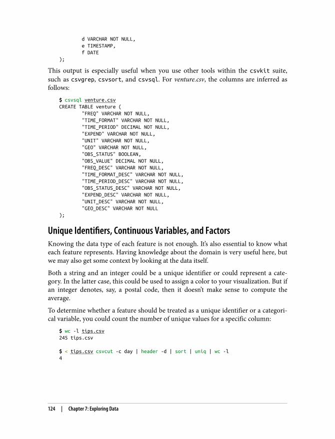
d VARCHAR NOT NULL, e TIMESTAMP, f DATE);

This output is especially useful when you use other tools within the csvkit suite,such as csvgrep, csvsort, and csvsql. For venture.csv, the columns are inferred asfollows:

$ csvsql venture.csvCREATE TABLE venture ( "FREQ" VARCHAR NOT NULL, "TIME_FORMAT" VARCHAR NOT NULL, "TIME_PERIOD" DECIMAL NOT NULL, "EXPEND" VARCHAR NOT NULL, "UNIT" VARCHAR NOT NULL, "GEO" VARCHAR NOT NULL, "OBS_STATUS" BOOLEAN, "OBS_VALUE" DECIMAL NOT NULL, "FREQ_DESC" VARCHAR NOT NULL, "TIME_FORMAT_DESC" VARCHAR NOT NULL, "TIME_PERIOD_DESC" VARCHAR NOT NULL, "OBS_STATUS_DESC" VARCHAR NOT NULL, "EXPEND_DESC" VARCHAR NOT NULL, "UNIT_DESC" VARCHAR NOT NULL, "GEO_DESC" VARCHAR NOT NULL);

Unique Identifiers, Continuous Variables, and FactorsKnowing the data type of each feature is not enough. It’s also essential to know whateach feature represents. Having knowledge about the domain is very useful here, butwe may also get some context by looking at the data itself.

Both a string and an integer could be a unique identifier or could represent a cate‐gory. In the latter case, this could be used to assign a color to your visualization. But ifan integer denotes, say, a postal code, then it doesn’t make sense to compute theaverage.

To determine whether a feature should be treated as a unique identifier or a categori‐cal variable, you could count the number of unique values for a specific column:

$ wc -l tips.csv245 tips.csv $ < tips.csv csvcut -c day | header -d | sort | uniq | wc -l4

124 | Chapter 7: Exploring Data

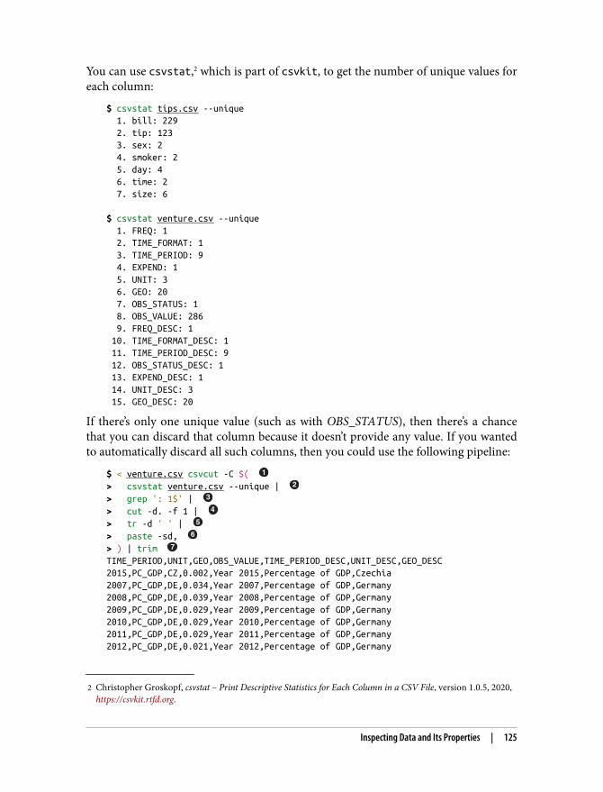
2 Christopher Groskopf, csvstat – Print Descriptive Statistics for Each Column in a CSV File, version 1.0.5, 2020,https://csvkit.rtfd.org.

You can use csvstat,2 which is part of csvkit, to get the number of unique values foreach column:

$ csvstat tips.csv --unique 1. bill: 229 2. tip: 123 3. sex: 2 4. smoker: 2 5. day: 4 6. time: 2 7. size: 6 $ csvstat venture.csv --unique 1. FREQ: 1 2. TIME_FORMAT: 1 3. TIME_PERIOD: 9 4. EXPEND: 1 5. UNIT: 3 6. GEO: 20 7. OBS_STATUS: 1 8. OBS_VALUE: 286 9. FREQ_DESC: 1 10. TIME_FORMAT_DESC: 1 11. TIME_PERIOD_DESC: 9 12. OBS_STATUS_DESC: 1 13. EXPEND_DESC: 1 14. UNIT_DESC: 3 15. GEO_DESC: 20

If there’s only one unique value (such as with OBS_STATUS), then there’s a chancethat you can discard that column because it doesn’t provide any value. If you wantedto automatically discard all such columns, then you could use the following pipeline:

$ < venture.csv csvcut -C $( > csvstat venture.csv --unique | > grep ': 1$' | > cut -d. -f 1 | > tr -d ' ' | > paste -sd, > ) | trim TIME_PERIOD,UNIT,GEO,OBS_VALUE,TIME_PERIOD_DESC,UNIT_DESC,GEO_DESC2015,PC_GDP,CZ,0.002,Year 2015,Percentage of GDP,Czechia2007,PC_GDP,DE,0.034,Year 2007,Percentage of GDP,Germany2008,PC_GDP,DE,0.039,Year 2008,Percentage of GDP,Germany2009,PC_GDP,DE,0.029,Year 2009,Percentage of GDP,Germany2010,PC_GDP,DE,0.029,Year 2010,Percentage of GDP,Germany2011,PC_GDP,DE,0.029,Year 2011,Percentage of GDP,Germany2012,PC_GDP,DE,0.021,Year 2012,Percentage of GDP,Germany

Inspecting Data and Its Properties | 125

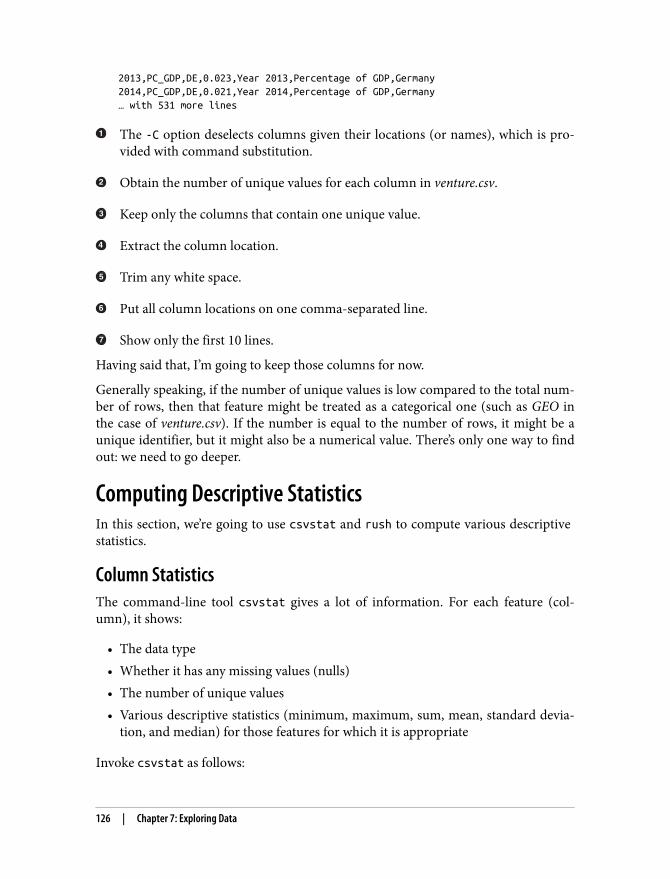
2013,PC_GDP,DE,0.023,Year 2013,Percentage of GDP,Germany2014,PC_GDP,DE,0.021,Year 2014,Percentage of GDP,Germany… with 531 more lines

The -C option deselects columns given their locations (or names), which is pro‐vided with command substitution.

Obtain the number of unique values for each column in venture.csv.

Keep only the columns that contain one unique value.

Extract the column location.

Trim any white space.

Put all column locations on one comma-separated line.

Show only the first 10 lines.

Having said that, I’m going to keep those columns for now.

Generally speaking, if the number of unique values is low compared to the total num‐ber of rows, then that feature might be treated as a categorical one (such as GEO inthe case of venture.csv). If the number is equal to the number of rows, it might be aunique identifier, but it might also be a numerical value. There’s only one way to findout: we need to go deeper.

Computing Descriptive StatisticsIn this section, we’re going to use csvstat and rush to compute various descriptive statistics.

Column StatisticsThe command-line tool csvstat gives a lot of information. For each feature (col‐umn), it shows:

• The data type• Whether it has any missing values (nulls)• The number of unique values• Various descriptive statistics (minimum, maximum, sum, mean, standard devia‐

tion, and median) for those features for which it is appropriate

Invoke csvstat as follows:

126 | Chapter 7: Exploring Data

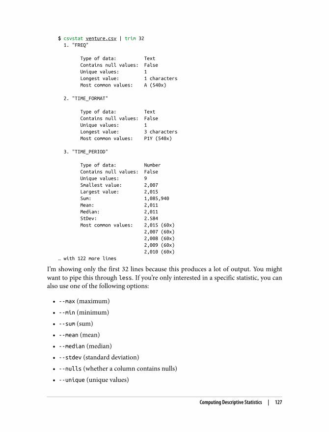
$ csvstat venture.csv | trim 32 1. "FREQ" Type of data: Text Contains null values: False Unique values: 1 Longest value: 1 characters Most common values: A (540x) 2. "TIME_FORMAT" Type of data: Text Contains null values: False Unique values: 1 Longest value: 3 characters Most common values: P1Y (540x) 3. "TIME_PERIOD" Type of data: Number Contains null values: False Unique values: 9 Smallest value: 2,007 Largest value: 2,015 Sum: 1,085,940 Mean: 2,011 Median: 2,011 StDev: 2.584 Most common values: 2,015 (60x) 2,007 (60x) 2,008 (60x) 2,009 (60x) 2,010 (60x)… with 122 more lines

I’m showing only the first 32 lines because this produces a lot of output. You mightwant to pipe this through less. If you’re only interested in a specific statistic, you canalso use one of the following options:

• --max (maximum)• --min (minimum)• --sum (sum)• --mean (mean)• --median (median)• --stdev (standard deviation)• --nulls (whether a column contains nulls)• --unique (unique values)

Computing Descriptive Statistics | 127

• --freq (frequent values)• --len (maximum value length)

For example:

$ csvstat venture.csv --freq | trim 1. FREQ: { "A": 540 } 2. TIME_FORMAT: { "P1Y": 540 } 3. TIME_PERIOD: { "2015": 60, "2007": 60, "2008": 60, "2009": 60, "2010": 60 } 4. EXPEND: { "INV_VEN": 540 } 5. UNIT: { "PC_GDP": 180, "NR_COMP": 180, "MIO_EUR": 180 } 6. GEO: { "CZ": 27, "DE": 27, "DK": 27, "EL": 27, "ES": 27 } 7. OBS_STATUS: { "None": 540 } 8. OBS_VALUE: { "0": 28, "1": 19, "2": 14, "0.002": 10, "0.034": 7 } 9. FREQ_DESC: { "Annual": 540 } 10. TIME_FORMAT_DESC: { "Annual": 540 }… with 5 more lines

You can select a subset of features with the -c option, which accepts both integers andcolumn names:

$ csvstat venture.csv -c 3,GEO 3. "TIME_PERIOD" Type of data: Number Contains null values: False Unique values: 9 Smallest value: 2,007 Largest value: 2,015 Sum: 1,085,940 Mean: 2,011 Median: 2,011 StDev: 2.584 Most common values: 2,015 (60x) 2,007 (60x) 2,008 (60x) 2,009 (60x) 2,010 (60x) 6. "GEO" Type of data: Text Contains null values: False Unique values: 20 Longest value: 2 characters Most common values: CZ (27x) DE (27x) DK (27x) EL (27x) ES (27x) Row count: 540

128 | Chapter 7: Exploring Data

3 The R Foundation for Statistical Computing, R – a Language and Environment for Statistical Computing, ver‐sion 4.0.4, 2021, https://www.r-project.org.

Keep in mind that csvstat, just like csvsql, employs heuristics todetermine the data type and therefore may not always get it right. Iencourage you to always do a manual inspection, as discussed inthe previous subsection. Moreover, even though the type may be astring or an integer, that doesn’t say anything about how it shouldbe used.

As a nice extra, csvstat outputs, at the very end, the number of data points (rows).Newlines and commas inside values are handled correctly. To see only that last line,you can use tail. Alternatively, you can use xsv, which returns only the actual num‐ber of rows:

$ csvstat venture.csv | tail -n 1Row count: 540 $ xsv count venture.csv540

Note that using either of these two options is different from using wc -l, whichcounts the number of newlines (and therefore also counts the header).

R One-Liners on the ShellIn this section I’d like to discuss the command-line tool rush, which enables you toleverage the statistical programming environment R3 directly from the command line.Before I explain what rush does and why it exists, let’s talk a bit about R itself.

R is a very powerful statistical software package for doing data science. It’s an inter‐preted programming language, has an extensive collection of packages, and offers itsown REPL, which, similar to the command line, allows you to play with your data.Note that once you start R, you’re in an interactive session that is separated from theUnix command line.

Imagine that you have a CSV file called tips.csv, and you would like compute the tippercentage and save the result. To accomplish this in R, you would first run R:

$ R --quiet >

I use the --quiet option here to suppress the rather long startup message.

And then run the following code:

Computing Descriptive Statistics | 129

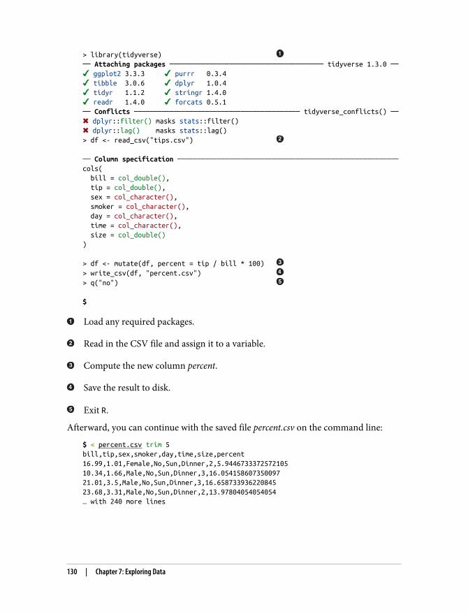
> library(tidyverse) ── Attaching packages ─────────────────────────────────────── tidyverse 1.3.0 ──✔ ggplot2 3.3.3 ✔ purrr 0.3.4✔ tibble 3.0.6 ✔ dplyr 1.0.4✔ tidyr 1.1.2 ✔ stringr 1.4.0✔ readr 1.4.0 ✔ forcats 0.5.1── Conflicts ────────────────────────────────────────── tidyverse_conflicts() ──✖ dplyr::filter() masks stats::filter()✖ dplyr::lag() masks stats::lag()> df <- read_csv("tips.csv") ── Column specification ────────────────────────────────────────────────────────cols( bill = col_double(), tip = col_double(), sex = col_character(), smoker = col_character(), day = col_character(), time = col_character(), size = col_double()) > df <- mutate(df, percent = tip / bill * 100) > write_csv(df, "percent.csv") > q("no") $

Load any required packages.

Read in the CSV file and assign it to a variable.

Compute the new column percent.

Save the result to disk.

Exit R.

Afterward, you can continue with the saved file percent.csv on the command line:

$ < percent.csv trim 5bill,tip,sex,smoker,day,time,size,percent16.99,1.01,Female,No,Sun,Dinner,2,5.944673337257210510.34,1.66,Male,No,Sun,Dinner,3,16.05415860735009721.01,3.5,Male,No,Sun,Dinner,3,16.65873393622084523.68,3.31,Male,No,Sun,Dinner,2,13.97804054054054… with 240 more lines

130 | Chapter 7: Exploring Data

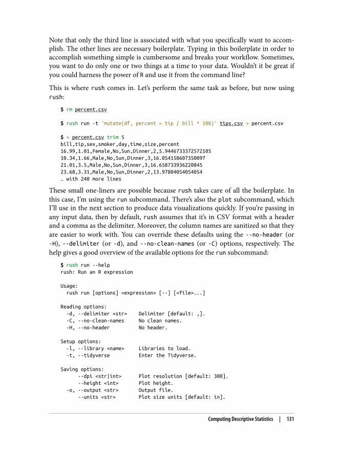
Note that only the third line is associated with what you specifically want to accom‐plish. The other lines are necessary boilerplate. Typing in this boilerplate in order toaccomplish something simple is cumbersome and breaks your workflow. Sometimes,you want to do only one or two things at a time to your data. Wouldn’t it be great ifyou could harness the power of R and use it from the command line?

This is where rush comes in. Let’s perform the same task as before, but now usingrush:

$ rm percent.csv $ rush run -t 'mutate(df, percent = tip / bill * 100)' tips.csv > percent.csv $ < percent.csv trim 5bill,tip,sex,smoker,day,time,size,percent16.99,1.01,Female,No,Sun,Dinner,2,5.944673337257210510.34,1.66,Male,No,Sun,Dinner,3,16.05415860735009721.01,3.5,Male,No,Sun,Dinner,3,16.65873393622084523.68,3.31,Male,No,Sun,Dinner,2,13.97804054054054… with 240 more lines

These small one-liners are possible because rush takes care of all the boilerplate. Inthis case, I’m using the run subcommand. There’s also the plot subcommand, whichI’ll use in the next section to produce data visualizations quickly. If you’re passing inany input data, then by default, rush assumes that it’s in CSV format with a headerand a comma as the delimiter. Moreover, the column names are sanitized so that theyare easier to work with. You can override these defaults using the --no-header (or-H), --delimiter (or -d), and --no-clean-names (or -C) options, respectively. Thehelp gives a good overview of the available options for the run subcommand:

$ rush run --helprush: Run an R expression Usage: rush run [options] <expression> [--] [<file>...] Reading options: -d, --delimiter <str> Delimiter [default: ,]. -C, --no-clean-names No clean names. -H, --no-header No header. Setup options: -l, --library <name> Libraries to load. -t, --tidyverse Enter the Tidyverse. Saving options: --dpi <str|int> Plot resolution [default: 300]. --height <int> Plot height. -o, --output <str> Output file. --units <str> Plot size units [default: in].

Computing Descriptive Statistics | 131

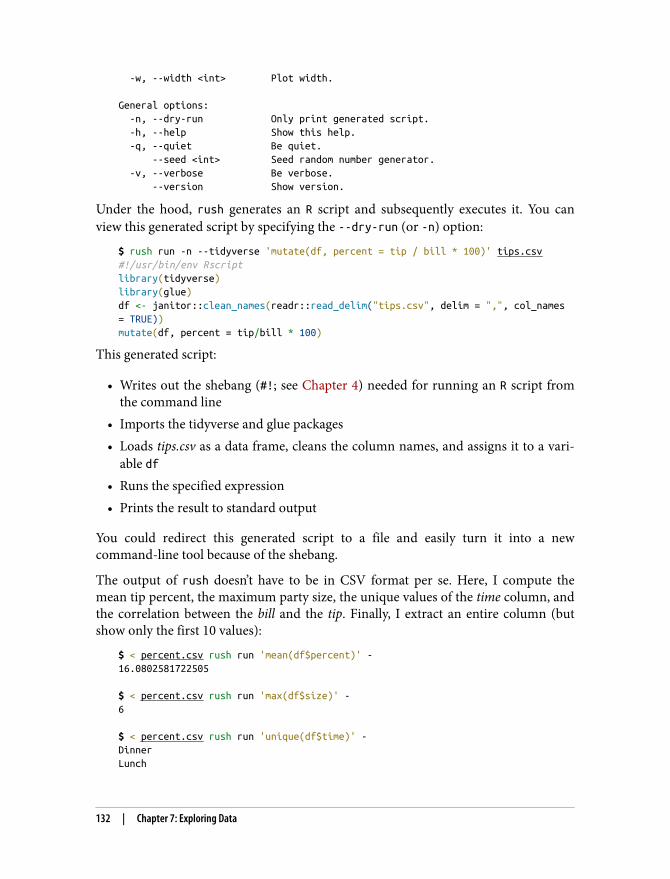
-w, --width <int> Plot width. General options: -n, --dry-run Only print generated script. -h, --help Show this help. -q, --quiet Be quiet. --seed <int> Seed random number generator. -v, --verbose Be verbose. --version Show version.

Under the hood, rush generates an R script and subsequently executes it. You canview this generated script by specifying the --dry-run (or -n) option:

$ rush run -n --tidyverse 'mutate(df, percent = tip / bill * 100)' tips.csv#!/usr/bin/env Rscriptlibrary(tidyverse)library(glue)df <- janitor::clean_names(readr::read_delim("tips.csv", delim = ",", col_names= TRUE))mutate(df, percent = tip/bill * 100)

This generated script:

• Writes out the shebang (#!; see Chapter 4) needed for running an R script fromthe command line

• Imports the tidyverse and glue packages• Loads tips.csv as a data frame, cleans the column names, and assigns it to a vari‐

able df• Runs the specified expression• Prints the result to standard output

You could redirect this generated script to a file and easily turn it into a newcommand-line tool because of the shebang.

The output of rush doesn’t have to be in CSV format per se. Here, I compute themean tip percent, the maximum party size, the unique values of the time column, andthe correlation between the bill and the tip. Finally, I extract an entire column (butshow only the first 10 values):

$ < percent.csv rush run 'mean(df$percent)' -16.0802581722505 $ < percent.csv rush run 'max(df$size)' -6 $ < percent.csv rush run 'unique(df$time)' -DinnerLunch

132 | Chapter 7: Exploring Data

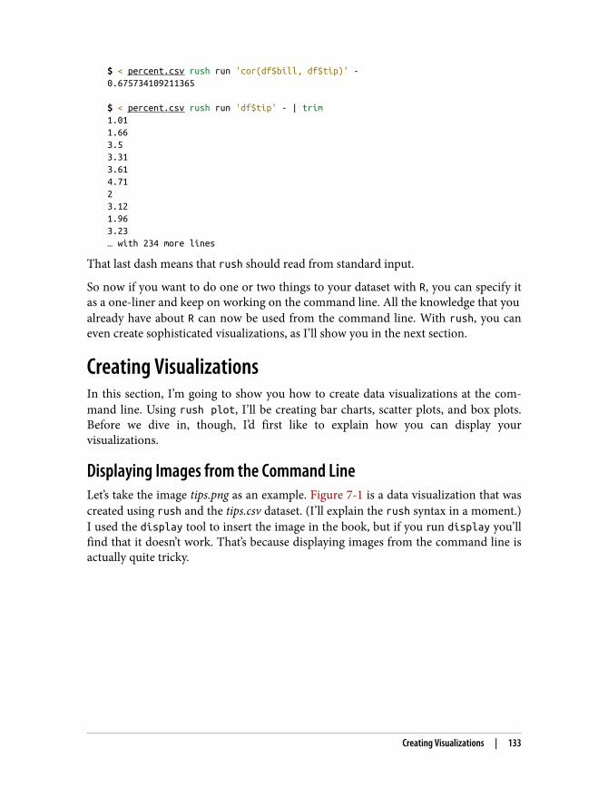
$ < percent.csv rush run 'cor(df$bill, df$tip)' -0.675734109211365 $ < percent.csv rush run 'df$tip' - | trim1.011.663.53.313.614.7123.121.963.23… with 234 more lines

That last dash means that rush should read from standard input.

So now if you want to do one or two things to your dataset with R, you can specify itas a one-liner and keep on working on the command line. All the knowledge that you already have about R can now be used from the command line. With rush, you caneven create sophisticated visualizations, as I’ll show you in the next section.

Creating VisualizationsIn this section, I’m going to show you how to create data visualizations at the com‐mand line. Using rush plot, I’ll be creating bar charts, scatter plots, and box plots.Before we dive in, though, I’d first like to explain how you can display yourvisualizations.

Displaying Images from the Command LineLet’s take the image tips.png as an example. Figure 7-1 is a data visualization that wascreated using rush and the tips.csv dataset. (I’ll explain the rush syntax in a moment.)I used the display tool to insert the image in the book, but if you run display you’llfind that it doesn’t work. That’s because displaying images from the command line isactually quite tricky.

Creating Visualizations | 133

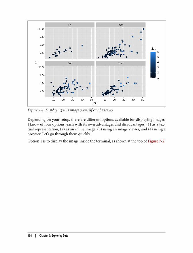
Figure 7-1. Displaying this image yourself can be tricky

Depending on your setup, there are different options available for displaying images.I know of four options, each with its own advantages and disadvantages: (1) as a tex‐tual representation, (2) as an inline image, (3) using an image viewer, and (4) using abrowser. Let’s go through them quickly.

Option 1 is to display the image inside the terminal, as shown at the top of Figure 7-2.

134 | Chapter 7: Exploring Data

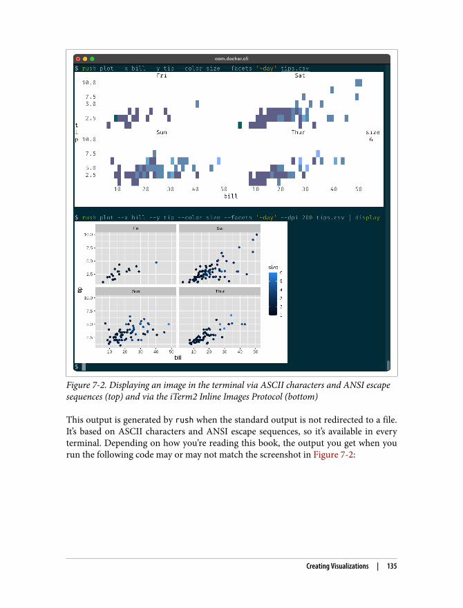
Figure 7-2. Displaying an image in the terminal via ASCII characters and ANSI escapesequences (top) and via the iTerm2 Inline Images Protocol (bottom)

This output is generated by rush when the standard output is not redirected to a file.It’s based on ASCII characters and ANSI escape sequences, so it’s available in everyterminal. Depending on how you’re reading this book, the output you get when yourun the following code may or may not match the screenshot in Figure 7-2:

Creating Visualizations | 135

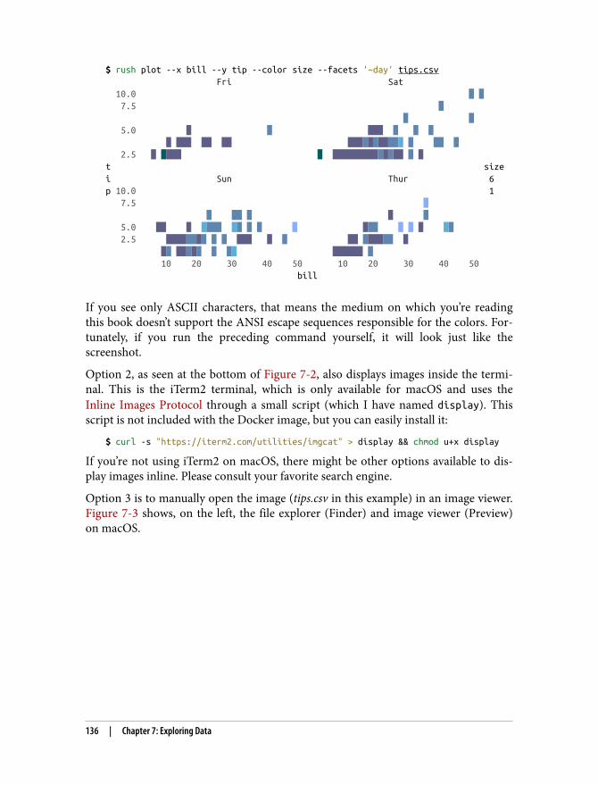
$ rush plot --x bill --y tip --color size --facets '~day' tips.csv Fri Sat 10.0 * # 7.5 * # * 5.0 # * ### * # # # ### ## ## #####*####+ * ** # 2.5 # %### % #########*#*## # # t size i Sun Thur 6 p 10.0 1 7.5 = * ** * # * 5.0 ## # +#*# +* * # = ##* = = # +* 2.5 ######## # * ### # # ## #####* # ## ####* * #+ ###### # 10 20 30 40 50 10 20 30 40 50 bill

If you see only ASCII characters, that means the medium on which you’re readingthis book doesn’t support the ANSI escape sequences responsible for the colors. For‐tunately, if you run the preceding command yourself, it will look just like thescreenshot.

Option 2, as seen at the bottom of Figure 7-2, also displays images inside the termi‐nal. This is the iTerm2 terminal, which is only available for macOS and uses theInline Images Protocol through a small script (which I have named display). Thisscript is not included with the Docker image, but you can easily install it:

$ curl -s "https://iterm2.com/utilities/imgcat" > display && chmod u+x display

If you’re not using iTerm2 on macOS, there might be other options available to dis‐play images inline. Please consult your favorite search engine.

Option 3 is to manually open the image (tips.csv in this example) in an image viewer.Figure 7-3 shows, on the left, the file explorer (Finder) and image viewer (Preview)on macOS.

136 | Chapter 7: Exploring Data

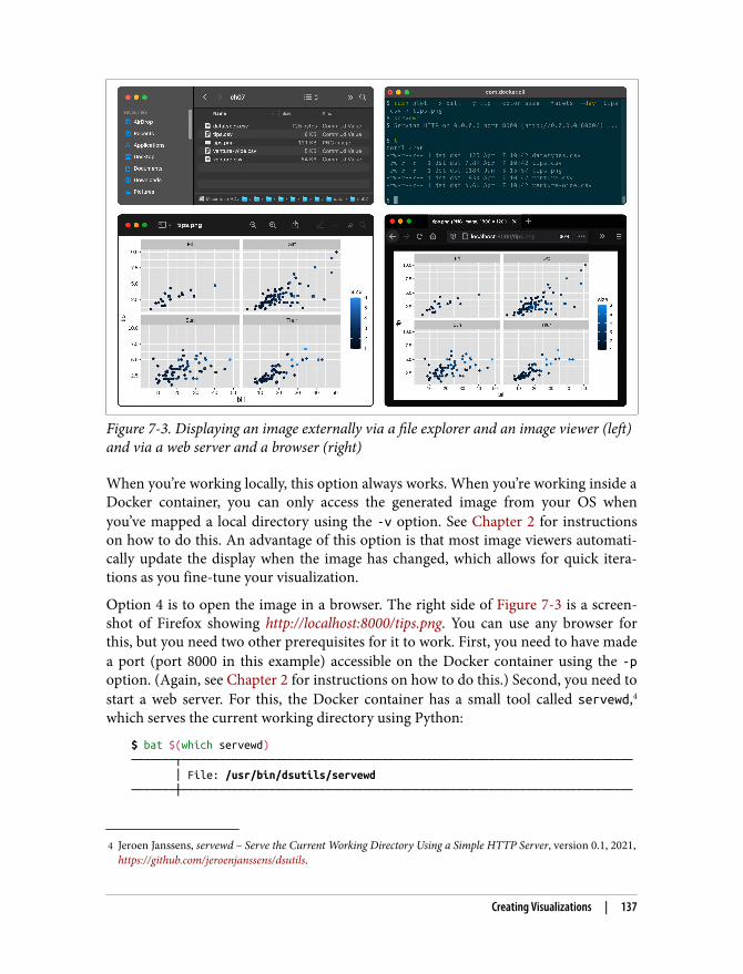
4 Jeroen Janssens, servewd – Serve the Current Working Directory Using a Simple HTTP Server, version 0.1, 2021,https://github.com/jeroenjanssens/dsutils.

Figure 7-3. Displaying an image externally via a file explorer and an image viewer (left)and via a web server and a browser (right)

When you’re working locally, this option always works. When you’re working inside aDocker container, you can only access the generated image from your OS whenyou’ve mapped a local directory using the -v option. See Chapter 2 for instructionson how to do this. An advantage of this option is that most image viewers automati‐cally update the display when the image has changed, which allows for quick itera‐tions as you fine-tune your visualization.

Option 4 is to open the image in a browser. The right side of Figure 7-3 is a screen‐shot of Firefox showing http://localhost:8000/tips.png. You can use any browser forthis, but you need two other prerequisites for it to work. First, you need to have madea port (port 8000 in this example) accessible on the Docker container using the -poption. (Again, see Chapter 2 for instructions on how to do this.) Second, you need tostart a web server. For this, the Docker container has a small tool called servewd,4

which serves the current working directory using Python:

$ bat $(which servewd)───────┬──────────────────────────────────────────────────────────────────────── │ File: /usr/bin/dsutils/servewd───────┼────────────────────────────────────────────────────────────────────────

Creating Visualizations | 137

1 │ #!/usr/bin/env bash 2 │ ARGS="$@" 3 │ python3 -m http.server ${ARGS} 2>/dev/null &───────┴────────────────────────────────────────────────────────────────────────

You only need to run servewd once from a directory (/data/, for example), and it willhappily run in the background. Once you’ve plotted something, you can visit local‐host:8000 in your browser and access the contents of that directory and all of its sub‐directories. The default port is 8000, but you can change this by specifying it as anargument to servewd:

$ servewd 9999 > display

Just make sure that this port is accessible. Because servewd runs in the background,you need to stop it as follows:

$ pkill -f http.server

Option 4 can also work on a remote machine.

Now that we’ve covered four options for displaying images, let’s move on to actuallycreating some.

Plotting in a RushWhen it comes to creating data visualizations, there’s a plethora of options. Person‐ally, I’m a staunch proponent of ggplot2, which is a visualization package for R. Theunderlying grammar of graphics is accompanied by a consistent API that allows youto quickly and iteratively create different types of beautiful data visualizations whilerarely having to consult the documentation—a welcoming set of properties whenexploring data.

We’re not really in a rush, but we also don’t want to fiddle too much with any singlevisualization. Moreover, we’d like to stay at the command line as much as possible.Luckily, we still have rush, which allows us to use ggplot2 from the command line.The data visualization in Figure 7-1 could have been created as follows:

$ rush run --library ggplot2 'ggplot(df, aes(x = bill, y = tip, color = size)) + geom_point() + facet_wrap(~day)' tips.csv > tips.png

However, as you may have noticed, I have used a very different command to createtips.png:

$ rush plot --x bill --y tip --color size --facets '~day' tips.csv > tips.png

While the syntax of ggplot2 is relatively concise, especially considering the flexibilityit offers, there’s a shortcut to create basic plots quickly. This shortcut is availablethrough the plot subcommand of rush, and it allows you to create beautiful basicplots without needing to learn R and the grammar of graphics.

138 | Chapter 7: Exploring Data

Under the hood, rush plot uses the function qplot from the ggplot2 package. Here’sthe first part of qplot’s documentation:

$ R -q -e '?ggplot2::qplot' | trim 14> ?ggplot2::qplotqplot package:ggplot2 R Documentation Quick plot Description: ‘qplot()’ is a shortcut designed to be familiar if you're used to base ‘plot()’. It's a convenient wrapper for creating a number of different types of plots using a consistent calling scheme. It's great for allowing you to produce plots quickly, but I highly recommend learning ‘ggplot()’ as it makes it easier to create complex graphics. … with 108 more lines

I agree with this advice; once you’re done reading this book, you’ll find it worthwhileto learn ggplot2, especially if you want to upgrade any exploratory data visualizationsinto ones that are suitable for communication. For now, while we’re at the commandline, let’s take that shortcut.

As Figure 7-2 already showed, rush plot can create both graphical visualizations(consisting of pixels) and textual visualizations (consisting of ASCII characters andANSI escape sequences) with the same syntax. When rush detects that its output hasbeen piped to another command such as display, or redirected to a file such astips.png, it will produce a graphical visualization; otherwise, it will produce a textualvisualization.

Let’s take a moment to read through the plotting and saving options of rush plot:

$ rush plot --helprush: Quick plot Usage: rush plot [options] [--] [<file>|-] Reading options: -d, --delimiter <str> Delimiter [default: ,]. -C, --no-clean-names No clean names. -H, --no-header No header. Setup options: -l, --library <name> Libraries to load. -t, --tidyverse Enter the Tidyverse. Plotting options: --aes <key=value> Additional aesthetics.

Creating Visualizations | 139

-a, --alpha <name> Alpha column. -c, --color <name> Color column. --facets <formula> Facet specification. -f, --fill <name> Fill column. -g, --geom <geom> Geometry [default: auto]. --group <name> Group column. --log <x|y|xy> Variables to log transform. --margins Display marginal facets. --post <code> Code to run after plotting. --pre <code> Code to run before plotting. --shape <name> Shape column. --size <name> Size column. --title <str> Plot title. -x, --x <name> X column. --xlab <str> X axis label. -y, --y <name> Y column. --ylab <str> Y axis label. -z, --z <name> Z column. Saving options: --dpi <str|int> Plot resolution [default: 300]. --height <int> Plot height. -o, --output <str> Output file. --units <str> Plot size units [default: in]. -w, --width <int> Plot width. General options: -n, --dry-run Only print generated script. -h, --help Show this help. -q, --quiet Be quiet. --seed <int> Seed random number generator. -v, --verbose Be verbose. --version Show version.

The most important options are the plotting options that take a <name> as an argu‐ment. For example, the --x option allows you to specify which column should beused to determine where things should be placed along the x-axis. The same holds forthe --y option. The --color and --fill options are used to specify which columnyou want to use for coloring. You can probably guess what the --size and --alphaoptions are about. Other common options are explained throughout the sections as Icreate various visualizations. Note that for each visualization, I first show its textualrepresentation (ASCII and ANSI characters) and then its visual representation(pixels).

Creating Bar ChartsBar charts are especially useful for displaying the value counts of a categorical feature.Here’s a textual visualization of the time feature in the tips.csv dataset:

140 | Chapter 7: Exploring Data

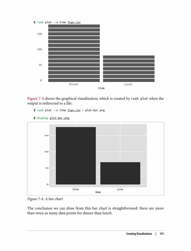
$ rush plot --x time tips.csv ******************************** ******************************** 150 ******************************** ******************************** ******************************** ******************************** 100 ******************************** ******************************** ******************************** ******************************** ******************************** ******************************** 50 ******************************** ******************************** ******************************** ******************************** ******************************** ******************************** ******************************** ******************************** 0 ******************************** ******************************** Dinner Lunch time

Figure 7-4 shows the graphical visualization, which is created by rush plot when theoutput is redirected to a file:

$ rush plot --x time tips.csv > plot-bar.png $ display plot-bar.png

Figure 7-4. A bar chart

The conclusion we can draw from this bar chart is straightforward: there are morethan twice as many data points for dinner than lunch.

Creating Visualizations | 141

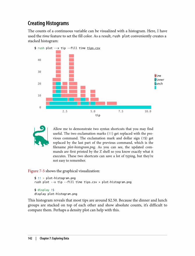
Creating HistogramsThe counts of a continuous variable can be visualized with a histogram. Here, I haveused the time feature to set the fill color. As a result, rush plot conveniently creates a stacked histogram:

$ rush plot --x tip --fill time tips.csv === === === 40 === === === === === === 30 === === === === time ===== === Dinner 20 ==+++ === ===== Lunch ==+++==== ===== === + ==+++==== ===== === === 10 +++++========== === === ====+++++++++=+++====+++== ===== ==+++++++++++++++++==+++++=+++====== ====== 0 ++++++++++++++++++++++++++++++++++++++++++++++++++++++++++++++++ 2.5 5.0 7.5 10.0 tip

Allow me to demonstrate two syntax shortcuts that you may finduseful. The two exclamation marks (!!) get replaced with the pre‐vious command. The exclamation mark and dollar sign (!$) getreplaced by the last part of the previous command, which is thefilename plot-histogram.png. As you can see, the updated com‐mands are first printed by the Z shell so you know exactly what itexecutes. These two shortcuts can save a lot of typing, but they’renot easy to remember.

Figure 7-5 shows the graphical visualization:

$ !! > plot-histogram.pngrush plot --x tip --fill time tips.csv > plot-histogram.png $ display !$display plot-histogram.png

This histogram reveals that most tips are around $2.50. Because the dinner and lunchgroups are stacked on top of each other and show absolute counts, it’s difficult tocompare them. Perhaps a density plot can help with this.

142 | Chapter 7: Exploring Data

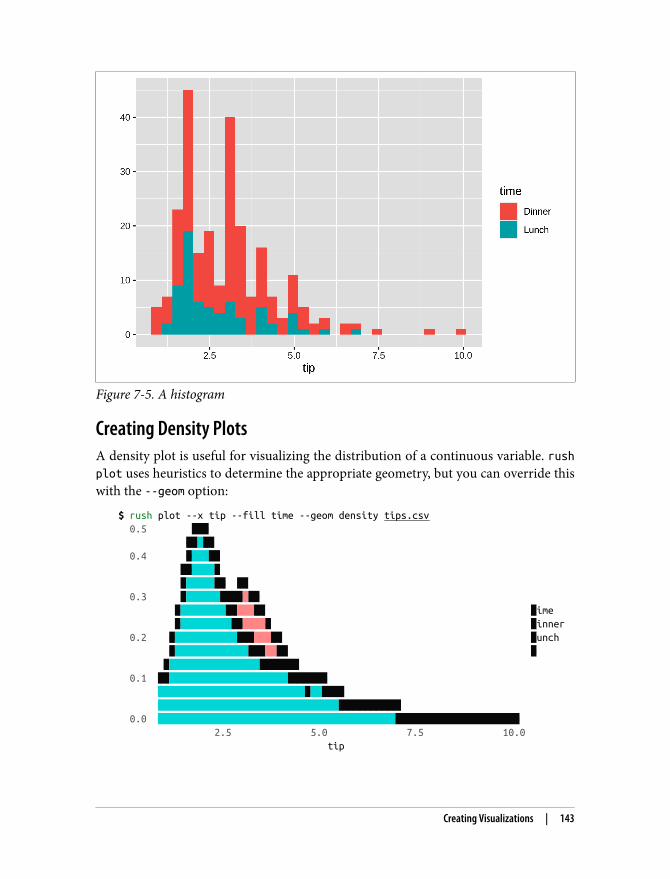
Figure 7-5. A histogram

Creating Density PlotsA density plot is useful for visualizing the distribution of a continuous variable. rushplot uses heuristics to determine the appropriate geometry, but you can override thiswith the --geom option:

$ rush plot --x tip --fill time --geom density tips.csv 0.5 @@@ @@+@@ 0.4 @+++@@ @@++++@ @+++++@@ @@ 0.3 @++++++@@@@=@@ @++++++++@@===@@ time @+++++++++@@====@ Dinner 0.2 @+++++++++++@@@===@@ Lunch @+++++++++++++@@@==@@ @ @++++++++++++++++@@@@@@@ 0.1 @@+++++++++++++++++++++@@@@@@@ ++++++++++++++++++++++++++@++@@@@ ++++++++++++++++++++++++++++++++@@@@@@@@@@@ 0.0 ++++++++++++++++++++++++++++++++++++++++++@@@@@@@@@@@@@@@@@@@@@@ 2.5 5.0 7.5 10.0 tip

Creating Visualizations | 143

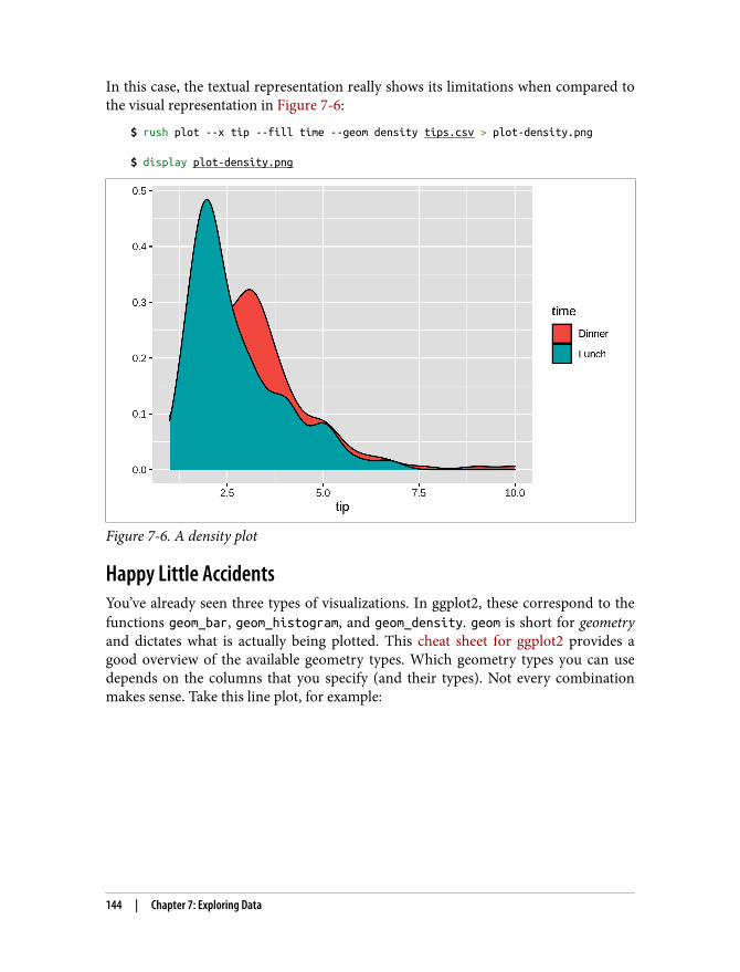
In this case, the textual representation really shows its limitations when compared tothe visual representation in Figure 7-6:

$ rush plot --x tip --fill time --geom density tips.csv > plot-density.png $ display plot-density.png

Figure 7-6. A density plot

Happy Little AccidentsYou’ve already seen three types of visualizations. In ggplot2, these correspond to thefunctions geom_bar, geom_histogram, and geom_density. geom is short for geometryand dictates what is actually being plotted. This cheat sheet for ggplot2 provides agood overview of the available geometry types. Which geometry types you can usedepends on the columns that you specify (and their types). Not every combinationmakes sense. Take this line plot, for example:

144 | Chapter 7: Exploring Data

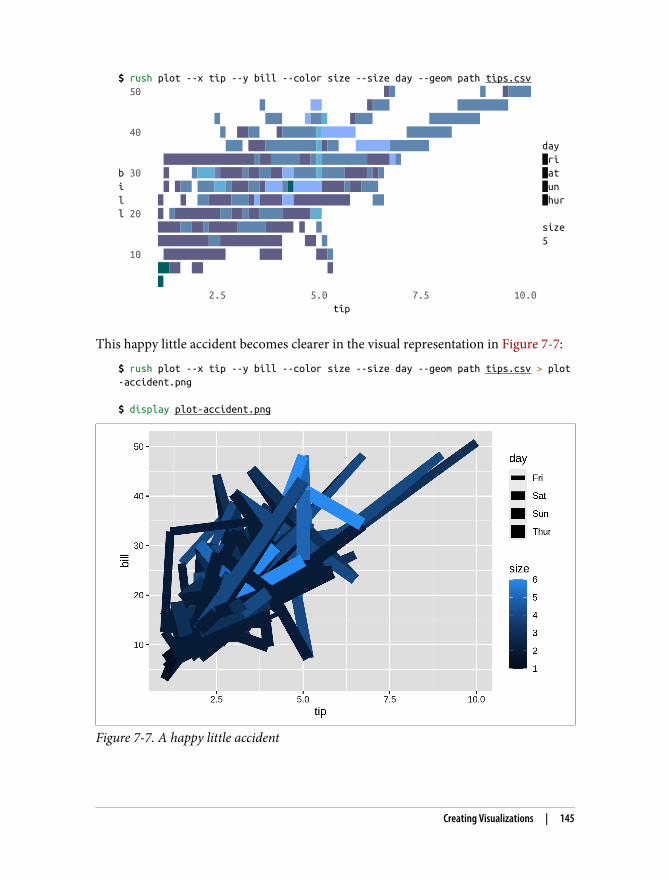
$ rush plot --x tip --y bill --color size --size day --geom path tips.csv 50 #* * ##### # == #*** ****##### # ### =**+ #*** *****#### 40 # ##** ####***+====== *****### #*# ###******###+#** ======****### day ###################*****##*+*##*****####=# Fri b 30 # *+++########**##==****+****####### Sat i # #** *##++####**#===*%=====####*##**# Sun l # # ######***#=####==########## ** Thur l 20 # #########**#####****#####++ ########*########*###### # * size ###################### ## * 5 10 ########### #### ##* %%## ## # % 2.5 5.0 7.5 10.0 tip

This happy little accident becomes clearer in the visual representation in Figure 7-7:

$ rush plot --x tip --y bill --color size --size day --geom path tips.csv > plot-accident.png $ display plot-accident.png

Figure 7-7. A happy little accident

Creating Visualizations | 145

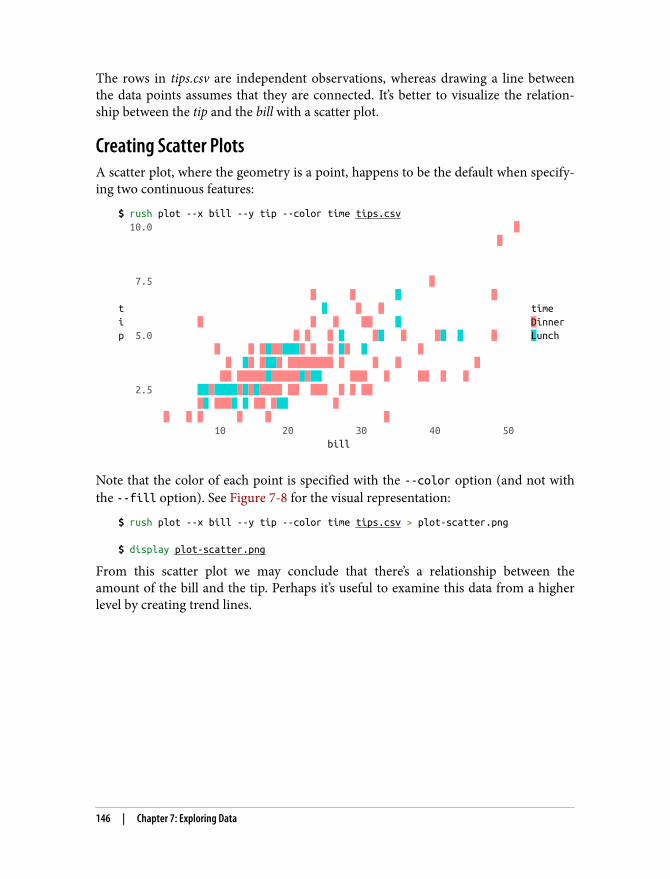
The rows in tips.csv are independent observations, whereas drawing a line betweenthe data points assumes that they are connected. It’s better to visualize the relation‐ship between the tip and the bill with a scatter plot.

Creating Scatter PlotsA scatter plot, where the geometry is a point, happens to be the default when specify‐ing two continuous features:

$ rush plot --x bill --y tip --color time tips.csv 10.0 = = 7.5 = = = + = t + = = time i = = = == + Dinner p 5.0 = = = + =+ = =+ + = Lunch = = =+==+++= = = += + = = += =++= ======== = = = = == =====+=====+=++ === = == = = 2.5 ++=++++=+=+==== == === = = == =+ ===+ + == =++ = = = = = = = 10 20 30 40 50 bill

Note that the color of each point is specified with the --color option (and not withthe --fill option). See Figure 7-8 for the visual representation:

$ rush plot --x bill --y tip --color time tips.csv > plot-scatter.png $ display plot-scatter.png

From this scatter plot we may conclude that there’s a relationship between theamount of the bill and the tip. Perhaps it’s useful to examine this data from a higherlevel by creating trend lines.

146 | Chapter 7: Exploring Data

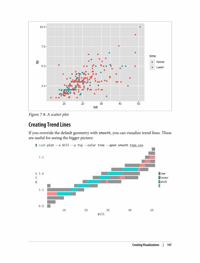
Figure 7-8. A scatter plot

Creating Trend LinesIf you override the default geometry with smooth, you can visualize trend lines. Theseare useful for seeing the bigger picture:

$ rush plot --x bill --y tip --color time --geom smooth tips.csv == ==== 7.5 ====== ======== ================== =======+++++++++====== t 5.0 ====+++++++++========== time i ====++++++================= Dinner p ===+++++++============= Lunch == ==+++++++===== = 2.5 ==============++++==== ======++++++++=== ========== ===== 0.0 == 10 20 30 40 50 bill

Creating Visualizations | 147

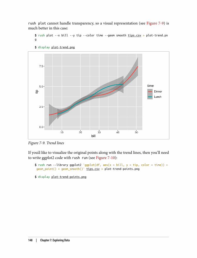
rush plot cannot handle transparency, so a visual representation (see Figure 7-9) ismuch better in this case:

$ rush plot --x bill --y tip --color time --geom smooth tips.csv > plot-trend.png $ display plot-trend.png

Figure 7-9. Trend lines

If you’d like to visualize the original points along with the trend lines, then you’ll needto write ggplot2 code with rush run (see Figure 7-10):

$ rush run --library ggplot2 'ggplot(df, aes(x = bill, y = tip, color = time)) + geom_point() + geom_smooth()' tips.csv > plot-trend-points.png $ display plot-trend-points.png

148 | Chapter 7: Exploring Data

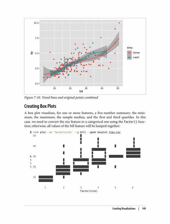
Figure 7-10. Trend lines and original points combined

Creating Box PlotsA box plot visualizes, for one or more features, a five-number summary: the mini‐mum, the maximum, the sample median, and the first and third quartiles. In thiscase, we need to convert the size feature to a categorical one using the factor() func‐tion; otherwise, all values of the bill feature will be lumped together:

$ rush plot --x 'factor(size)' --y bill --geom boxplot tips.csv 50 % % % % % % % 40 % % % % % %%%%%%%%%% %%%%%%%%%% % % % % %%%%%%%%%% b 30 % % % %%%%%%%%%% %%%%%%%%%% i % %%%%%%%%%%% %%%%%%%%%% l % % % %%%%%%%%%% l 20 %%%%%%%%%% %%%%%%%%%%% % % %%%%%%%%%% %%%%%%%%%%% %%%%%%%%%% % 10 %%%%%%%%%% % %%%%%%%%%% 1 2 3 4 5 6 factor(size)

Creating Visualizations | 149

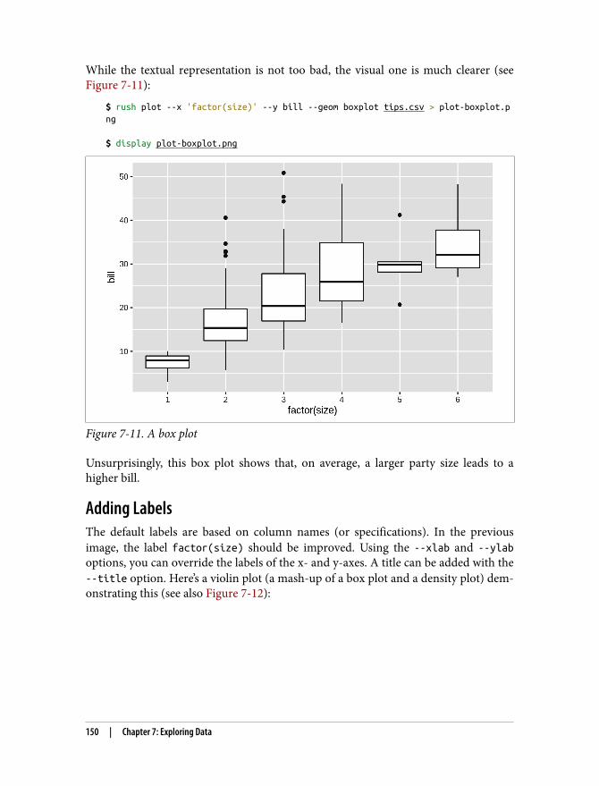
While the textual representation is not too bad, the visual one is much clearer (seeFigure 7-11):

$ rush plot --x 'factor(size)' --y bill --geom boxplot tips.csv > plot-boxplot.png $ display plot-boxplot.png

Figure 7-11. A box plot

Unsurprisingly, this box plot shows that, on average, a larger party size leads to ahigher bill.

Adding LabelsThe default labels are based on column names (or specifications). In the previousimage, the label factor(size) should be improved. Using the --xlab and --ylaboptions, you can override the labels of the x- and y-axes. A title can be added with the--title option. Here’s a violin plot (a mash-up of a box plot and a density plot) dem‐onstrating this (see also Figure 7-12):

150 | Chapter 7: Exploring Data

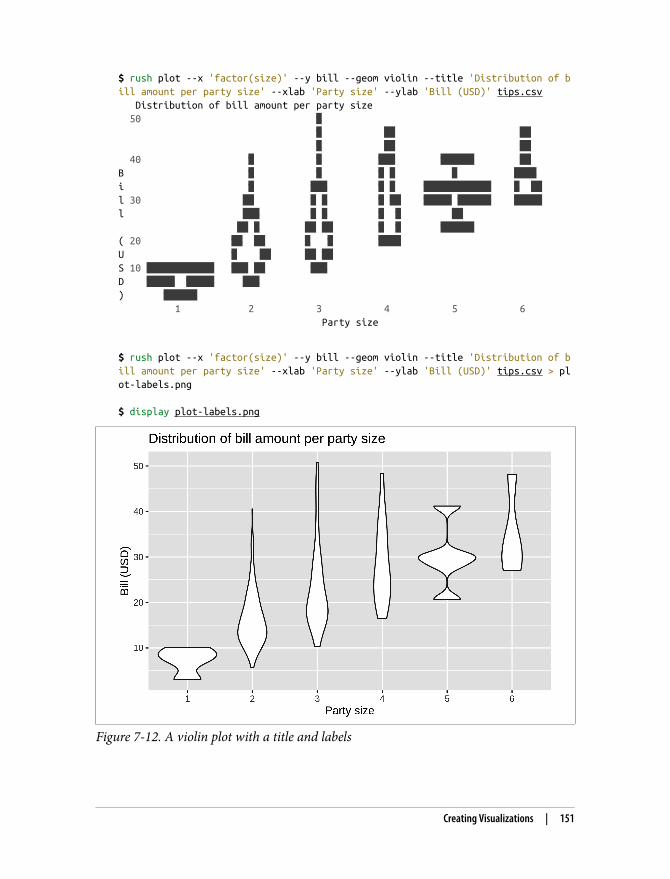
$ rush plot --x 'factor(size)' --y bill --geom violin --title 'Distribution of bill amount per party size' --xlab 'Party size' --ylab 'Bill (USD)' tips.csv Distribution of bill amount per party size 50 % % %% %% % %% %% 40 % % %%% %%%%%% %% B % % % % % %%%% i % %%% % % %%%%%%%%%%%% % %% l 30 %% % % % %% %%%%% %%%%%% %%%%% l %%% % % % % %% %% % %% %% % % %%%%%% ( 20 %% %% % % %%%% U % %% %% %% S 10 %%%%%%%%%%%% %%% %% %%% D %%%%% %%%%% %%% ) %%%%%% 1 2 3 4 5 6 Party size

$ rush plot --x 'factor(size)' --y bill --geom violin --title 'Distribution of bill amount per party size' --xlab 'Party size' --ylab 'Bill (USD)' tips.csv > plot-labels.png $ display plot-labels.png

Figure 7-12. A violin plot with a title and labels

Creating Visualizations | 151

Annotating your visualization with proper labels and a title is especially useful if youwant to share it with others (or your future self), as they will make it easier to under‐stand what’s being shown.

Going Beyond Basic PlotsAlthough rush plot is suitable for creating basic plots when you’re exploring data, itcertainly has its limitations. Sometimes you need more flexibility and sophisticatedoptions such as multiple geometries, coordinate transformations, and theming. Inthat case, it might be worthwhile to learn more about the underlying package fromwhich rush plot draws its capabilities, namely the ggplot2 package for R. If you’remore into Python than R, there’s the plotnine package, which is a reimplementationof ggplot2 for Python.

SummaryIn this chapter we’ve looked at various ways to explore your data. Both textual andgraphical data visualizations have their pros and cons. The graphical ones are obvi‐ously of much higher quality but can be tricky to view at the command line. This iswhere textual visualizations come in handy. At least rush, thanks to R and ggplot2,has a consistent syntax for creating both types.

The next chapter is yet another intermezzo chapter in which I discuss how you canspeed up your commands and pipelines. Feel free to read that chapter later if youcan’t wait to start modeling your data in Chapter 9.

For Further Exploration• A proper ggplot2 tutorial is unfortunately beyond the scope of this book. If you

want to get better at visualizing your data, I strongly recommend that you investsome time in understanding the power and beauty of the grammar of graphics.Chapters 3 and 28 of the book R for Data Science by Hadley Wickham and Gar‐rett Grolemund (O’Reilly) are an excellent resource.

• Speaking of Chapters 3 and 28, I translated those to Python using plotnine andPandas, in case you’re more into Python than R.

152 | Chapter 7: Exploring Data

CHAPTER 8

Parallel Pipelines

In the previous chapters, we’ve been dealing with commands and pipelines that takecare of an entire task at once. In practice, however, you may find yourself facing a taskthat requires the same command or pipeline to run multiple times. For example, youmay need to:

• Scrape hundreds of web pages• Make dozens of API calls and transform their output• Train a classifier for a range of parameter values• Generate scatter plots for every pair of features in your dataset

In any of these examples, there’s a certain form of repetition involved. With yourfavorite scripting or programming language, you could take care of this with a forloop or a while loop. On the command line, the first thing you might be inclined todo is to press the up arrow key to bring back the previous command, modify it if nec‐essary, and press Enter to run the command again. This is fine to do two or threetimes, but imagine doing it dozens of times. Such an approach quickly becomes cum‐bersome, inefficient, and prone to errors. The good news is that you can write suchloops on the command line as well. That’s what this chapter is all about.

Sometimes, repeating a fast command again and again in succession (in a serial man‐ner) is sufficient. When you have multiple cores (and perhaps even multiplemachines), it would be nice to make use of those, especially when you’re faced with adata-intensive task. Using multiple cores or machines may reduce the total runningtime significantly. In this chapter I will introduce a very powerful tool called

153

1 Ole Tange, parallel – Build and Execute Shell Command Lines from Standard Input in Parallel, version20161222, 2016, https://www.gnu.org/software/parallel.

parallel1 that can take care of exactly this. It enables you to apply a command orpipeline for a range of arguments such as numbers, lines, and files. Plus, as the nameimplies, it allows you to run your commands in parallel.

OverviewThis intermezzo chapter discusses several approaches to speeding up tasks thatrequire commands and pipelines to be run many times. My main goal is to demon‐strate to you the flexibility and power of parallel. Because this tool can be combinedwith any other tool discussed in this book, it will change the way you use the com‐mand line for data science for the better. In this chapter, you’ll learn about:

• Running commands in serial to a range of numbers, lines, and files• Breaking a large task into several smaller tasks• Running pipelines in parallel• Distributing pipelines to multiple machines

This chapter starts with the following files:

$ cd /data/ch08 $ ltotal 20K-rw-r--r-- 1 dst dst 126 Jun 29 14:32 emails.txt-rw-r--r-- 1 dst dst 61 Jun 29 14:32 movies.txt-rwxr-xr-x 1 dst dst 125 Jun 29 14:32 slow.sh*-rw-r--r-- 1 dst dst 5.1K Jun 29 14:32 users.json

The instructions for getting these files are in Chapter 2. Any other files are eitherdownloaded or generated using command-line tools.

Serial ProcessingBefore I dive into parallelization, I want to briefly discuss looping in a serial fashion.It’s worthwhile to know how to do this because this functionality is always available,the syntax closely resembles looping in other programming languages, and it willreally make you appreciate parallel.

From the examples provided in the introduction of this chapter, we can distill threetypes of items to loop over: numbers, lines, and files. These three types of items willbe discussed in the next three subsections, respectively.

154 | Chapter 8: Parallel Pipelines

Looping Over NumbersImagine that you need to compute the square of every even integer between 0 and100. There’s a tool called bc that is a basic calculator you can pipe an equation to. Thecommand to compute the square of 4 looks as follows:

$ echo "4^2" | bc16

For a one-off calculation, this will do. However, as mentioned in the introduction,you would have to be crazy to press the up arrow key, change the number, and pressEnter 50 times! It would be better to let the shell do the hard work for you by using afor loop:

$ for i in {0..100..2} > do> echo "$i^2" | bc > done | trim04163664100144196256324… with 41 more lines

The Z shell has a feature called brace expansion, which transforms {0..100..2}into a list separated by spaces: 0 2 4 … 98 100. The variable i is assigned thevalue 0 in the first iteration, 1 in the second iteration, and so forth.

The value of this variable can be used by prefixing it with a dollar sign ($). Theshell will replace $i with its value before echo is executed. Note that there can bemore than one command between do and done.

Although the syntax may appear a bit odd compared to your favorite programminglanguage, it’s worth remembering this because it’s always available in the shell. I’llintroduce a better and more flexible way of repeating commands in a moment.

Serial Processing | 155

Looping Over LinesThe second type of item you can loop over is lines. These lines can come from eithera file or standard input. This is a very generic approach because the lines can containanything, including numbers, dates, and email addresses.

Imagine that you want to send an email to all your contacts. Let’s first generate somefake users using the free Random User Generator API:

$ curl -s "https://randomuser.me/api/1.2/?results=5&seed=dsatcl2e" > users.json $ < users.json jq -r '.results[].email' > emails $ bat emails───────┬──────────────────────────────────────────────────────────────────────── │ File: emails───────┼──────────────────────────────────────────────────────────────────────── 1 │ selma.andersen@example.com 2 │ kent.clark@example.com 3 │ ditmar.niehaus@example.com 4 │ benjamin.robinson@example.com 5 │ paulo.muller@example.com───────┴────────────────────────────────────────────────────────────────────────

You can loop over the lines from emails with a while loop:

$ while read line > do> echo "Sending invitation to ${line}." > done < emails Sending invitation to selma.andersen@example.com.Sending invitation to kent.clark@example.com.Sending invitation to ditmar.niehaus@example.com.Sending invitation to benjamin.robinson@example.com.Sending invitation to paulo.muller@example.com.

In this case you need to use a while loop, because the Z shell does not knowbeforehand how many lines the input consists of.

Although the curly braces around the line variable are not necessary in this case(since variable names cannot contain periods), including them is still goodpractice.

This redirection can also be placed before while.

You can also provide input to a while loop interactively by specifying the special filestandard input /dev/stdin. Press Ctrl-D when you are done:

$ while read line; do echo "You typed: ${line}."; done < /dev/stdinoneYou typed: one.

156 | Chapter 8: Parallel Pipelines

2 Eric B. Decker, James Youngman, and Kevin Dalley, find – Search for Files in a Directory Hierarchy, version4.7.0, 2019, https://www.gnu.org/software/findutils.

twoYou typed: two.threeYou typed: three.

This method, however, has the disadvantage that, once you press Enter, the com‐mands between do and done are run immediately for that line of input. There’s noturning back.

Looping Over FilesIn this section I discuss the third type of item that we often need to loop over: files.

To handle special characters, use globbing (i.e., pathname expansion) instead of ls:

$ for chapter in /data/*> do> echo "Processing Chapter ${chapter}."> doneProcessing Chapter /data/ch01.Processing Chapter /data/ch02.Processing Chapter /data/ch03.Processing Chapter /data/ch04.Processing Chapter /data/ch05.Processing Chapter /data/ch06.Processing Chapter /data/ch07.Processing Chapter /data/ch08.Processing Chapter /data/ch09.Processing Chapter /data/ch10.

Just as with brace expansion, the expression /data/* is first expanded into a list bythe Z shell before it’s processed by the for loop. A more elaborate alternative to listingfiles is find,2 which:

• Can traverse down directories• Allows for elaborate searching on properties such as size, access time, and

permissions• Handles special characters such as spaces and newlines

For example, the following find invocation lists all files located under the direc‐tory /data that have csv as their extension and are smaller than 2 KB:

$ find /data -type f -name '*.csv' -size -2k/data/ch03/tmnt-basic.csv/data/ch03/tmnt-missing-newline.csv

Serial Processing | 157

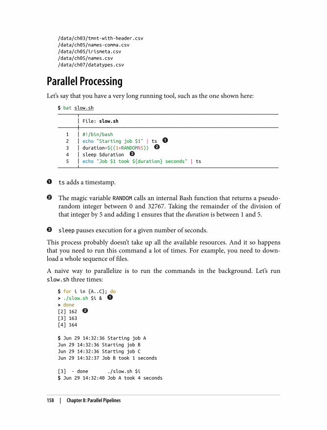
/data/ch03/tmnt-with-header.csv/data/ch05/names-comma.csv/data/ch05/irismeta.csv/data/ch05/names.csv/data/ch07/datatypes.csv

Parallel ProcessingLet’s say that you have a very long running tool, such as the one shown here:

$ bat slow.sh───────┬──────────────────────────────────────────────────────────────────────── │ File: slow.sh───────┼──────────────────────────────────────────────────────────────────────── 1 │ #!/bin/bash 2 │ echo "Starting job $1" | ts 3 │ duration=$((1+RANDOM%5)) 4 │ sleep $duration 5 │ echo "Job $1 took ${duration} seconds" | ts───────┴────────────────────────────────────────────────────────────────────────

ts adds a timestamp.

The magic variable RANDOM calls an internal Bash function that returns a pseudo‐random integer between 0 and 32767. Taking the remainder of the division ofthat integer by 5 and adding 1 ensures that the duration is between 1 and 5.

sleep pauses execution for a given number of seconds.

This process probably doesn’t take up all the available resources. And it so happensthat you need to run this command a lot of times. For example, you need to down‐load a whole sequence of files.

A naive way to parallelize is to run the commands in the background. Let’s runslow.sh three times:

$ for i in {A..C}; do> ./slow.sh $i & > done[2] 162 [3] 163[4] 164 $ Jun 29 14:32:36 Starting job AJun 29 14:32:36 Starting job BJun 29 14:32:36 Starting job CJun 29 14:32:37 Job B took 1 seconds [3] - done ./slow.sh $i$ Jun 29 14:32:40 Job A took 4 seconds

158 | Chapter 8: Parallel Pipelines

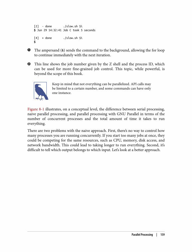
[2] - done ./slow.sh $i$ Jun 29 14:32:41 Job C took 5 seconds [4] + done ./slow.sh $i$

The ampersand (&) sends the command to the background, allowing the for loopto continue immediately with the next iteration.

This line shows the job number given by the Z shell and the process ID, whichcan be used for more fine-grained job control. This topic, while powerful, isbeyond the scope of this book.

Keep in mind that not everything can be parallelized. API calls maybe limited to a certain number, and some commands can have onlyone instance.

Figure 8-1 illustrates, on a conceptual level, the difference between serial processing,naive parallel processing, and parallel processing with GNU Parallel in terms of thenumber of concurrent processes and the total amount of time it takes to runeverything.

There are two problems with the naive approach. First, there’s no way to control howmany processes you are running concurrently. If you start too many jobs at once, theycould be competing for the same resources, such as CPU, memory, disk access, andnetwork bandwidth. This could lead to taking longer to run everything. Second, it’sdifficult to tell which output belongs to which input. Let’s look at a better approach.

Parallel Processing | 159

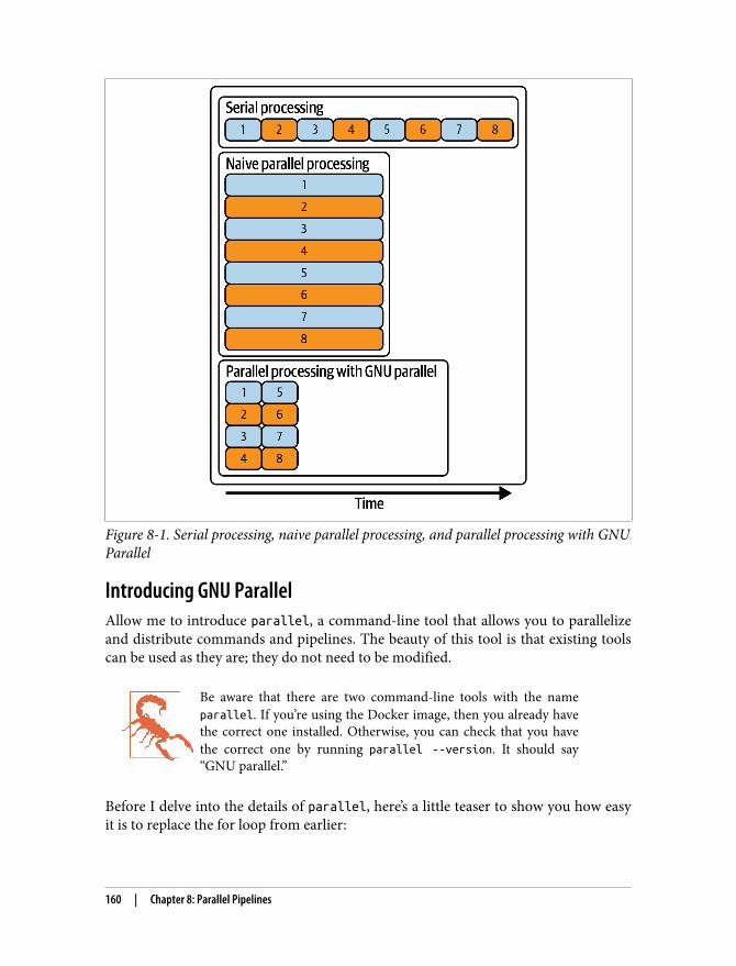
Figure 8-1. Serial processing, naive parallel processing, and parallel processing with GNUParallel

Introducing GNU ParallelAllow me to introduce parallel, a command-line tool that allows you to parallelizeand distribute commands and pipelines. The beauty of this tool is that existing toolscan be used as they are; they do not need to be modified.

Be aware that there are two command-line tools with the nameparallel. If you’re using the Docker image, then you already havethe correct one installed. Otherwise, you can check that you havethe correct one by running parallel --version. It should say“GNU parallel.”

Before I delve into the details of parallel, here’s a little teaser to show you how easyit is to replace the for loop from earlier:

160 | Chapter 8: Parallel Pipelines

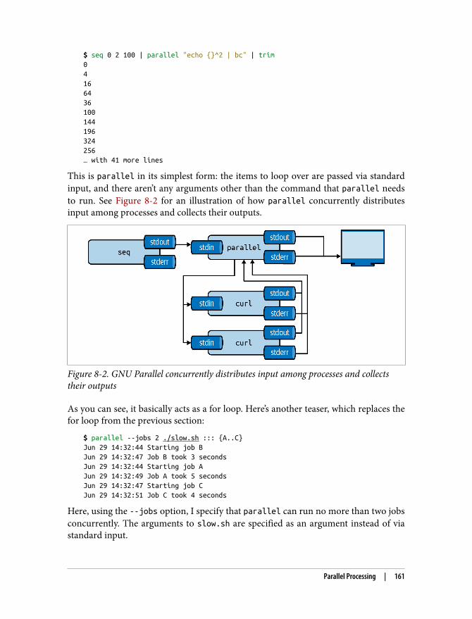
$ seq 0 2 100 | parallel "echo {}^2 | bc" | trim04166436100144196324256… with 41 more lines

This is parallel in its simplest form: the items to loop over are passed via standardinput, and there aren’t any arguments other than the command that parallel needsto run. See Figure 8-2 for an illustration of how parallel concurrently distributesinput among processes and collects their outputs.

Figure 8-2. GNU Parallel concurrently distributes input among processes and collectstheir outputs

As you can see, it basically acts as a for loop. Here’s another teaser, which replaces thefor loop from the previous section:

$ parallel --jobs 2 ./slow.sh ::: {A..C}Jun 29 14:32:44 Starting job BJun 29 14:32:47 Job B took 3 secondsJun 29 14:32:44 Starting job AJun 29 14:32:49 Job A took 5 secondsJun 29 14:32:47 Starting job CJun 29 14:32:51 Job C took 4 seconds

Here, using the --jobs option, I specify that parallel can run no more than two jobsconcurrently. The arguments to slow.sh are specified as an argument instead of viastandard input.

Parallel Processing | 161

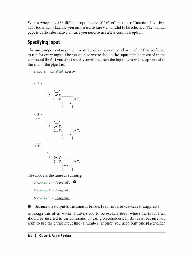
With a whopping 159 different options, parallel offers a lot of functionality. (Per‐haps too much.) Luckily, you only need to know a handful to be effective. The manualpage is quite informative, in case you need to use a less common option.

Specifying InputThe most important argument to parallel is the command or pipeline that you’d liketo run for every input. The question is: where should the input item be inserted in thecommand line? If you don’t specify anything, then the input item will be appended tothe end of the pipeline:

$ seq 3 | parallel cowsay ___< 1 > --- \ ^__^ \ (oo)\_______ (__)\ )\/\ ||----w | || || ___< 2 > --- \ ^__^ \ (oo)\_______ (__)\ )\/\ ||----w | || || ___< 3 > --- \ ^__^ \ (oo)\_______ (__)\ )\/\ ||----w | || ||

The above is the same as running:

$ cowsay 1 > /dev/null $ cowsay 2 > /dev/null $ cowsay 3 > /dev/null

Because the output is the same as before, I redirect it to /dev/null to suppress it.

Although this often works, I advise you to be explicit about where the input itemshould be inserted in the command by using placeholders. In this case, because youwant to use the entire input line (a number) at once, you need only one placeholder.

162 | Chapter 8: Parallel Pipelines

You specify the placeholder—that is, where to put the input item—with a pair of curlybraces ({}):

$ seq 3 | parallel cowsay {} > /dev/null

There are other ways to provide input to parallel. I prefer pipingthe input (as I do throughout this chapter) because that’s how mostcommand-line tools are chained together into a pipeline. The otherways involve syntax that’s not seen anywhere else. Having said that,they do enable additional functionality, such as iterating over allpossible combinations of multiple lists, so be sure to read parallel’s manual page if you’d like to know more.

When the input items are filenames, some modifiers allow you to use only a portionof the filename. For example, with {/}, only the basename of the filename will beused:

$ find /data/ch03 -type f | parallel echo '{#}\) \"{}\" has basename \"{/}\"' 1) "/data/ch03/tmnt-basic.csv" has basename "tmnt-basic.csv"2) "/data/ch03/top2000.xlsx" has basename "top2000.xlsx"3) "/data/ch03/r-datasets.db" has basename "r-datasets.db"4) "/data/ch03/tmnt-missing-newline.csv" has basename "tmnt-missing-newline.csv"5) "/data/ch03/tmnt-with-header.csv" has basename "tmnt-with-header.csv"6) "/data/ch03/logs.tar.gz" has basename "logs.tar.gz"

Characters such as parentheses ()) and quotes (") have a special meaning in theshell. To use them literally, you put a backslash (\) in front of them. This is calledescaping.

If the input line has multiple parts separated by a delimiter, you can add numbers tothe placeholders. For example:

$ < input.csv parallel --colsep , "mv {2} {1}" > /dev/null

Here, you can apply the same placeholder modifiers. It is also possible to reuse thesame input item. If the input to parallel is a CSV file with a header, then you canuse the column names as placeholders:

$ < input.csv parallel -C, --header : "invite {name} {email}"

If you ever start to wonder whether your placeholders are set upcorrectly, you can add the --dryrun option. Instead of actually exe‐cuting the commands, parallel will print out all the commandsexactly as if they have been executed.

Parallel Processing | 163

Controlling the Number of Concurrent JobsBy default, parallel runs one job per CPU core. You can control the number of jobsthat will be run concurrently with the --jobs or -j option. Specifying a number (N)means that many jobs will be run concurrently. If you put a plus sign in front of thenumber, then parallel will run N jobs plus the number of CPU cores. If you put aminus sign in front of the number, then parallel will run N – M jobs, where M is thenumber of CPU cores. You can also specify a percentage, where the default is 100% ofthe number of CPU cores. The optimal number of jobs to run concurrently dependson the actual commands you are running:

$ seq 5 | parallel -j0 "echo Hi {}"Hi 1Hi 2Hi 3Hi 4Hi 5

$ seq 5 | parallel -j200% "echo Hi {}"Hi 1Hi 2Hi 3Hi 4Hi 5

If you specify -j1, then the commands will be run in serial. Even though thisapproach doesn’t do the name of the tool justice, it still has its uses—for example,when you need to access an API that allows only one connection at a time. If youspecify -j0, then parallel will run as many jobs in parallel as possible. This can becompared to your for loop with the ampersand. Doing this is not advised.

Logging and OutputTo save the output of each command, you might be tempted to do the following:

$ seq 5 | parallel "echo \"Hi {}\" > hi-{}.txt"

This will save the output into individual files. Or if you want to save everything intoone big file, you could do the following:

$ seq 5 | parallel "echo Hi {}" >> one-big-file.txt

However, parallel offers the --results option, which stores the output in separatefiles. For each job, parallel creates three files: seq, which holds the job number;stdout, which contains the output produced by the job; and stderr, which contains anyerrors produced by the job. These three files are placed in subdirectories based on theinput values.

164 | Chapter 8: Parallel Pipelines

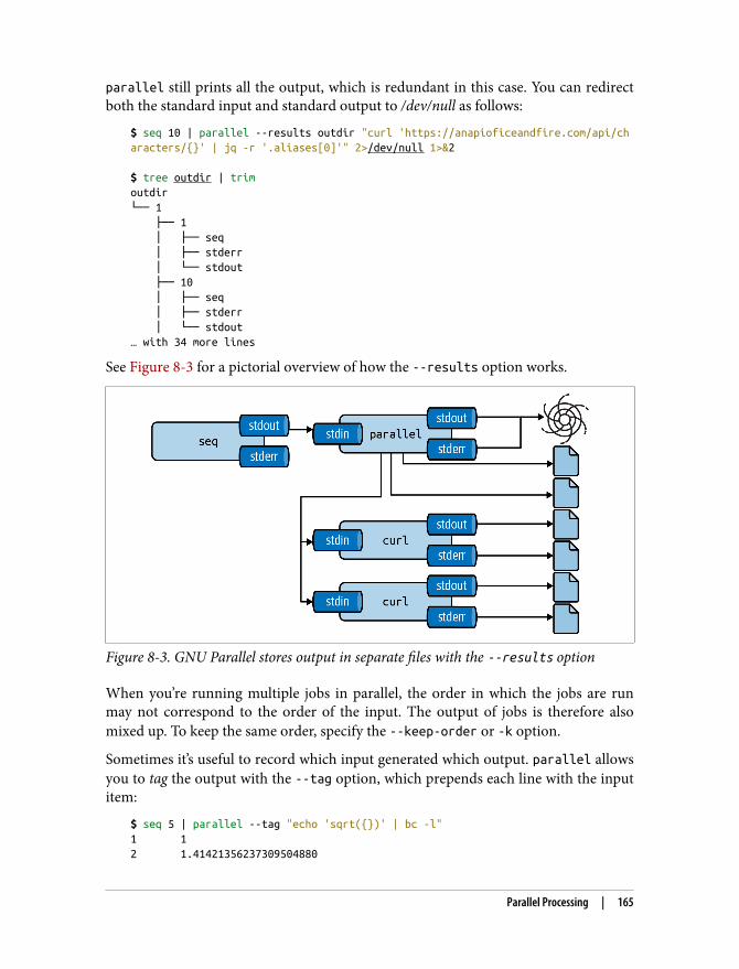
parallel still prints all the output, which is redundant in this case. You can redirectboth the standard input and standard output to /dev/null as follows:

$ seq 10 | parallel --results outdir "curl 'https://anapioficeandfire.com/api/characters/{}' | jq -r '.aliases[0]'" 2>/dev/null 1>&2 $ tree outdir | trimoutdir└── 1 ├── 1 │ ├── seq │ ├── stderr │ └── stdout ├── 10 │ ├── seq │ ├── stderr │ └── stdout… with 34 more lines

See Figure 8-3 for a pictorial overview of how the --results option works.

Figure 8-3. GNU Parallel stores output in separate files with the --results option

When you’re running multiple jobs in parallel, the order in which the jobs are runmay not correspond to the order of the input. The output of jobs is therefore alsomixed up. To keep the same order, specify the --keep-order or -k option.

Sometimes it’s useful to record which input generated which output. parallel allowsyou to tag the output with the --tag option, which prepends each line with the inputitem:

$ seq 5 | parallel --tag "echo 'sqrt({})' | bc -l"1 12 1.41421356237309504880

Parallel Processing | 165

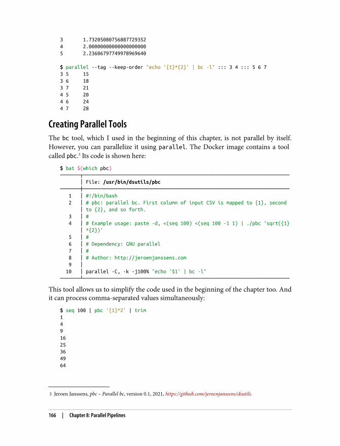
3 Jeroen Janssens, pbc – Parallel bc, version 0.1, 2021, https://github.com/jeroenjanssens/dsutils.

3 1.732050807568877293524 2.000000000000000000005 2.23606797749978969640 $ parallel --tag --keep-order "echo '{1}*{2}' | bc -l" ::: 3 4 ::: 5 6 73 5 153 6 183 7 214 5 204 6 244 7 28

Creating Parallel ToolsThe bc tool, which I used in the beginning of this chapter, is not parallel by itself.However, you can parallelize it using parallel. The Docker image contains a tool called pbc.3 Its code is shown here:

$ bat $(which pbc)───────┬──────────────────────────────────────────────────────────────────────── │ File: /usr/bin/dsutils/pbc───────┼──────────────────────────────────────────────────────────────────────── 1 │ #!/bin/bash 2 │ # pbc: parallel bc. First column of input CSV is mapped to {1}, second │ to {2}, and so forth. 3 │ # 4 │ # Example usage: paste -d, <(seq 100) <(seq 100 -1 1) | ./pbc 'sqrt({1} │ *{2})' 5 │ # 6 │ # Dependency: GNU parallel 7 │ # 8 │ # Author: http://jeroenjanssens.com 9 │ 10 │ parallel -C, -k -j100% "echo '$1' | bc -l"───────┴────────────────────────────────────────────────────────────────────────

This tool allows us to simplify the code used in the beginning of the chapter too. Andit can process comma-separated values simultaneously:

$ seq 100 | pbc '{1}^2' | trim1491625364964

166 | Chapter 8: Parallel Pipelines

81100… with 90 more lines $ paste -d, <(seq 4) <(seq 4) <(seq 4) | pbc 'sqrt({1}+{2})^{3}'1.414213562373095048804.0000000000000000000014.6969384566990685890563.99999999999999999969

Distributed ProcessingSometimes you need more power than your local machine, even with all its cores, canoffer. Luckily, parallel can also leverage the power of remote machines, which reallyallows you to speed up your pipeline.

What’s great is that parallel doesn’t have to be installed on the remote machine. Allthat’s required is that you’re able to connect to the remote machine with the SecureShell protocol (or SSH), which is also what parallel uses to distribute your pipeline.(Having parallel installed is helpful because it can then determine how many coresto employ on each remote machine; I’ll talk more about this later.)

First, we’re going to obtain a list of running Amazon Web Services’ Elastic ComputeCloud (AWS EC2) instances. Don’t worry if you don’t have any remote machines; youcan replace any occurrence of --slf hostnames, which tells parallel which remotemachines to use, with --sshlogin :. This way, you can still follow along with theexamples in this section.

Once you know which remote machines to take over, there are three flavors of dis‐tributed processing to consider:

• Running ordinary commands on remote machines• Distributing local data directly among remote machines• Sending files to remote machines, processing them, and retrieving the results

Get List of Running AWS EC2 InstancesIn this section, we’re creating a file named hostnames that will contain one hostnameof a remote machine per line. I’m using Amazon Web Services (AWS) as an example.I assume that you have an AWS account and that you know how to launch instances.If you’re using a different cloud computing service (such as Google Cloud Platform orMicrosoft Azure), or if you have your own servers, please make sure that you create ahostnames file yourself before continuing to the next section.

Distributed Processing | 167

4 Amazon Web Services, aws – Unified Tool to Manage AWS Services, version 2.1.32, 2021, https://aws.amazon.com/cli.

5 Tatu Ylonen et al., ssh – OpenSSH Remote Login Client, version 1:8.2p1-4ubuntu0.2, 2020, https://www.openssh.com.

You can obtain a list of running AWS EC2 instances using aws,4 the command-lineinterface to the AWS API. With aws, you can do almost everything you can do withthe online AWS Management Console.

The command aws ec2 describe-instances returns a lot of information about allyour EC2 instances in JSON format (see the online documentation for more informa‐tion). You can extract the relevant fields using jq:

$ aws ec2 describe-instances | jq '.Reservations[].Instances[] | {public_dns: .PublicDnsName, state: .State.Name}'

The possible states of an EC2 instance are pending, running, shutting-down,terminated, stopping, and stopped. Because you can only distribute your pipeline torunning instances, you filter out the nonrunning instances as follows:

> aws ec2 describe-instances | jq -r '.Reservations[].Instances[] | select(.State.Name=="running") | .PublicDnsName' | tee hostnamesec2-54-88-122-140.compute-1.amazonaws.comec2-54-88-89-208.compute-1.amazonaws.com

(Without the -r or --raw-output option, the hostnames would have been surroun‐ded by double quotes.) The output is saved to hostnames, so that I can pass this toparallel later.

As mentioned, parallel employs ssh5 to connect to the remote machines. If youwant to connect to your EC2 instances without typing the credentials every time, youcan add something like the following text to the file ~/.ssh/config:

$ bat ~/.ssh/config───────┬──────────────────────────────────────────────────────────────────────── │ File: /home/dst/.ssh/config───────┼──────────────────────────────────────────────────────────────────────── 1 │ Host *.amazonaws.com 2 │ IdentityFile ~/.ssh/MyKeyFile.pem 3 │ User ubuntu───────┴────────────────────────────────────────────────────────────────────────

Depending on which distribution you’re running, your username may be differentthan ubuntu.

168 | Chapter 8: Parallel Pipelines

6 Peter Tobias, Bernd Eckenfels, and Michael Meskes, hostname – Show or Set the System’s Host Name, version3.23, 2021, https://sourceforge.net/projects/net-tools/.

Running Commands on Remote MachinesThe first flavor of distributed processing is to run ordinary commands on remotemachines. Let’s first double-check that parallel is working by running the tool hostname6 on each EC2 instance:

$ parallel --nonall --sshloginfile hostnames hostnameip-172-31-23-204ip-172-31-23-205

Here, the --sshloginfile or --slf option is used to refer to the file hostnames. The--nonall option instructs parallel to execute the same command on every remotemachine in the hostnames file without using any parameters. Remember, if you don’thave any remote machines to utilize, you can replace --slf hostnames with--sshlogin : so that the command is run on your local machine:

$ parallel --nonall --sshlogin : hostnamedata-science-toolbox

Running the same command on every remote machine once requires only one coreper machine. If you wanted to distribute the list of arguments passed in to parallel,then it could potentially use more than one core. If it’s not specified explicitly,parallel will try to determine the number of cores:

$ seq 2 | parallel --slf hostnames echo 2>&1bash: parallel: command not foundparallel: Warning: Could not figure out number of cpus on ec2-54-88-122-140.compute-1.amazonaws.com (). Using 1.12

In this case, I have parallel installed on one of the two remote machines. I’m gettinga warning message indicating that parallel is not found on one of them. As a result,parallel cannot determine the number of cores and will default to using one core.When you receive this warning message, you can do one of the following four things:

• Don’t worry and be happy with using one core per machine.• Specify the number of jobs for each machine via the --jobs or -j option.• Specify the number of cores to use per machine by putting, for example, 2/ (if

you want two cores), in front of each hostname in the hostnames file.• Install parallel using a package manager—for example, if the remote machines

all run Ubuntu:

Distributed Processing | 169

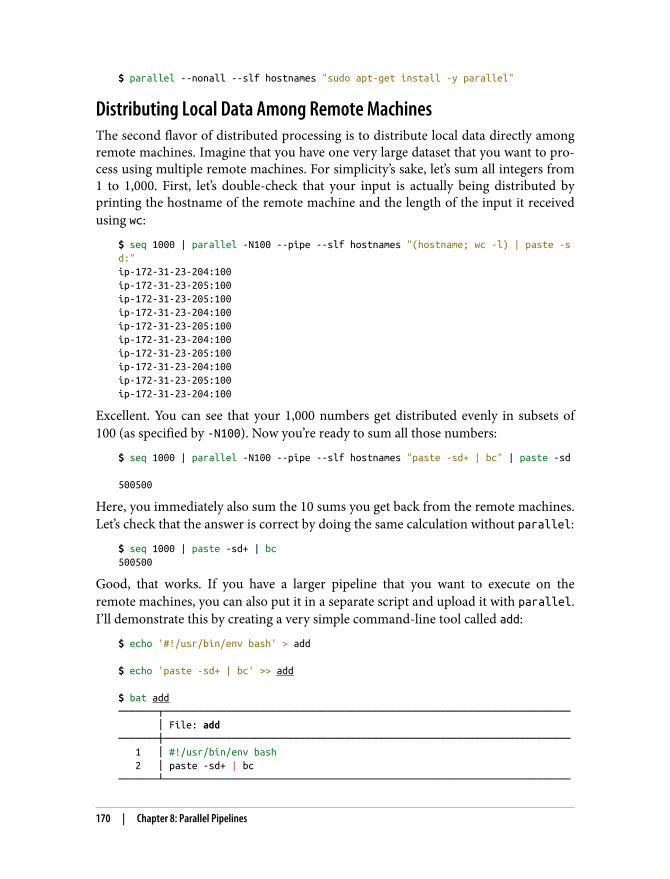
$ parallel --nonall --slf hostnames "sudo apt-get install -y parallel"

Distributing Local Data Among Remote MachinesThe second flavor of distributed processing is to distribute local data directly amongremote machines. Imagine that you have one very large dataset that you want to pro‐cess using multiple remote machines. For simplicity’s sake, let’s sum all integers from1 to 1,000. First, let’s double-check that your input is actually being distributed byprinting the hostname of the remote machine and the length of the input it receivedusing wc:

$ seq 1000 | parallel -N100 --pipe --slf hostnames "(hostname; wc -l) | paste -sd:"ip-172-31-23-204:100ip-172-31-23-205:100ip-172-31-23-205:100ip-172-31-23-204:100ip-172-31-23-205:100ip-172-31-23-204:100ip-172-31-23-205:100ip-172-31-23-204:100ip-172-31-23-205:100ip-172-31-23-204:100

Excellent. You can see that your 1,000 numbers get distributed evenly in subsets of100 (as specified by -N100). Now you’re ready to sum all those numbers:

$ seq 1000 | parallel -N100 --pipe --slf hostnames "paste -sd+ | bc" | paste -sd 500500

Here, you immediately also sum the 10 sums you get back from the remote machines.Let’s check that the answer is correct by doing the same calculation without parallel:

$ seq 1000 | paste -sd+ | bc500500

Good, that works. If you have a larger pipeline that you want to execute on theremote machines, you can also put it in a separate script and upload it with parallel.I’ll demonstrate this by creating a very simple command-line tool called add:

$ echo '#!/usr/bin/env bash' > add $ echo 'paste -sd+ | bc' >> add $ bat add───────┬──────────────────────────────────────────────────────────────────────── │ File: add───────┼──────────────────────────────────────────────────────────────────────── 1 │ #!/usr/bin/env bash 2 │ paste -sd+ | bc───────┴────────────────────────────────────────────────────────────────────────

170 | Chapter 8: Parallel Pipelines

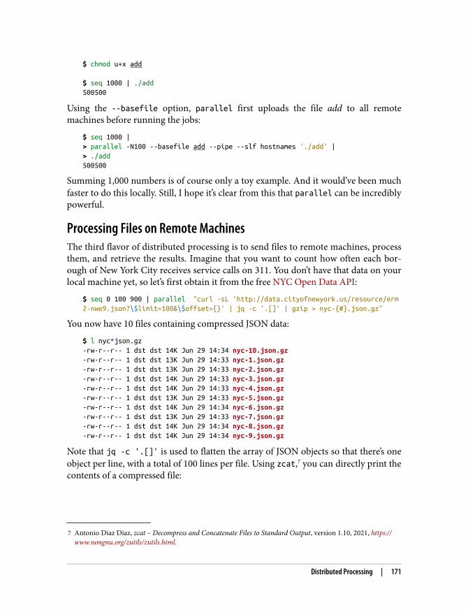
7 Antonio Diaz Diaz, zcat – Decompress and Concatenate Files to Standard Output, version 1.10, 2021, https://www.nongnu.org/zutils/zutils.html.

$ chmod u+x add $ seq 1000 | ./add500500

Using the --basefile option, parallel first uploads the file add to all remotemachines before running the jobs:

$ seq 1000 |> parallel -N100 --basefile add --pipe --slf hostnames './add' |> ./add500500

Summing 1,000 numbers is of course only a toy example. And it would’ve been muchfaster to do this locally. Still, I hope it’s clear from this that parallel can be incrediblypowerful.

Processing Files on Remote MachinesThe third flavor of distributed processing is to send files to remote machines, processthem, and retrieve the results. Imagine that you want to count how often each bor‐ough of New York City receives service calls on 311. You don’t have that data on yourlocal machine yet, so let’s first obtain it from the free NYC Open Data API:

$ seq 0 100 900 | parallel "curl -sL 'http://data.cityofnewyork.us/resource/erm2-nwe9.json?\$limit=100&\$offset={}' | jq -c '.[]' | gzip > nyc-{#}.json.gz"

You now have 10 files containing compressed JSON data:

$ l nyc*json.gz-rw-r--r-- 1 dst dst 14K Jun 29 14:34 nyc-10.json.gz-rw-r--r-- 1 dst dst 13K Jun 29 14:33 nyc-1.json.gz-rw-r--r-- 1 dst dst 13K Jun 29 14:33 nyc-2.json.gz-rw-r--r-- 1 dst dst 14K Jun 29 14:33 nyc-3.json.gz-rw-r--r-- 1 dst dst 14K Jun 29 14:33 nyc-4.json.gz-rw-r--r-- 1 dst dst 13K Jun 29 14:33 nyc-5.json.gz-rw-r--r-- 1 dst dst 14K Jun 29 14:34 nyc-6.json.gz-rw-r--r-- 1 dst dst 13K Jun 29 14:33 nyc-7.json.gz-rw-r--r-- 1 dst dst 14K Jun 29 14:34 nyc-8.json.gz-rw-r--r-- 1 dst dst 14K Jun 29 14:34 nyc-9.json.gz

Note that jq -c '.[]' is used to flatten the array of JSON objects so that there’s oneobject per line, with a total of 100 lines per file. Using zcat,7 you can directly print thecontents of a compressed file:

Distributed Processing | 171

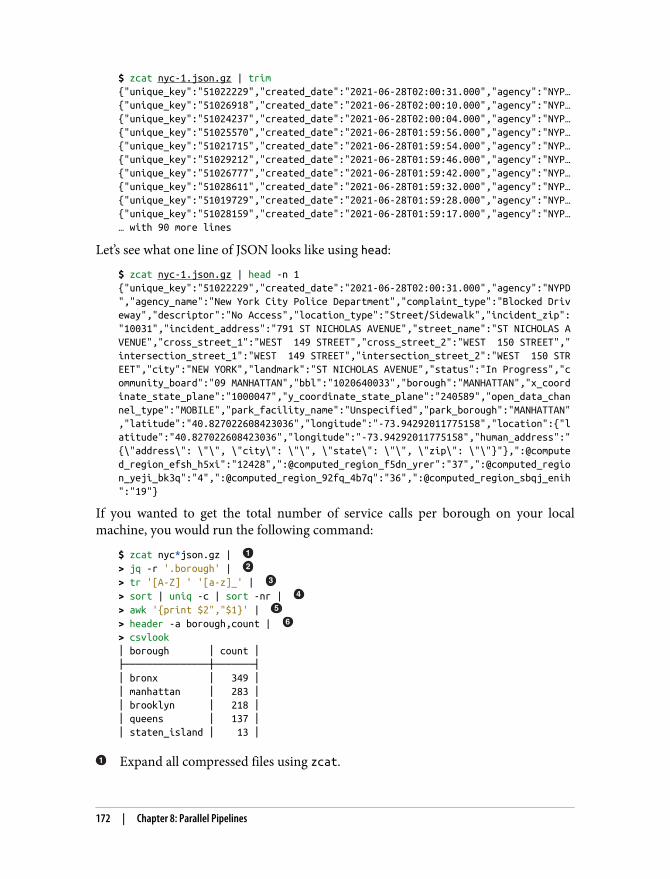
$ zcat nyc-1.json.gz | trim{"unique_key":"51022229","created_date":"2021-06-28T02:00:31.000","agency":"NYP…{"unique_key":"51026918","created_date":"2021-06-28T02:00:10.000","agency":"NYP…{"unique_key":"51024237","created_date":"2021-06-28T02:00:04.000","agency":"NYP…{"unique_key":"51025570","created_date":"2021-06-28T01:59:56.000","agency":"NYP…{"unique_key":"51021715","created_date":"2021-06-28T01:59:54.000","agency":"NYP…{"unique_key":"51029212","created_date":"2021-06-28T01:59:46.000","agency":"NYP…{"unique_key":"51026777","created_date":"2021-06-28T01:59:42.000","agency":"NYP…{"unique_key":"51028611","created_date":"2021-06-28T01:59:32.000","agency":"NYP…{"unique_key":"51019729","created_date":"2021-06-28T01:59:28.000","agency":"NYP…{"unique_key":"51028159","created_date":"2021-06-28T01:59:17.000","agency":"NYP…… with 90 more lines

Let’s see what one line of JSON looks like using head:

$ zcat nyc-1.json.gz | head -n 1{"unique_key":"51022229","created_date":"2021-06-28T02:00:31.000","agency":"NYPD","agency_name":"New York City Police Department","complaint_type":"Blocked Driveway","descriptor":"No Access","location_type":"Street/Sidewalk","incident_zip":"10031","incident_address":"791 ST NICHOLAS AVENUE","street_name":"ST NICHOLAS AVENUE","cross_street_1":"WEST 149 STREET","cross_street_2":"WEST 150 STREET","intersection_street_1":"WEST 149 STREET","intersection_street_2":"WEST 150 STREET","city":"NEW YORK","landmark":"ST NICHOLAS AVENUE","status":"In Progress","community_board":"09 MANHATTAN","bbl":"1020640033","borough":"MANHATTAN","x_coordinate_state_plane":"1000047","y_coordinate_state_plane":"240589","open_data_channel_type":"MOBILE","park_facility_name":"Unspecified","park_borough":"MANHATTAN","latitude":"40.827022608423036","longitude":"-73.94292011775158","location":{"latitude":"40.827022608423036","longitude":"-73.94292011775158","human_address":"{\"address\": \"\", \"city\": \"\", \"state\": \"\", \"zip\": \"\"}"},":@computed_region_efsh_h5xi":"12428",":@computed_region_f5dn_yrer":"37",":@computed_region_yeji_bk3q":"4",":@computed_region_92fq_4b7q":"36",":@computed_region_sbqj_enih":"19"}

If you wanted to get the total number of service calls per borough on your localmachine, you would run the following command:

$ zcat nyc*json.gz | > jq -r '.borough' | > tr '[A-Z] ' '[a-z]_' | > sort | uniq -c | sort -nr | > awk '{print $2","$1}' | > header -a borough,count | > csvlook│ borough │ count │├───────────────┼───────┤│ bronx │ 349 ││ manhattan │ 283 ││ brooklyn │ 218 ││ queens │ 137 ││ staten_island │ 13 │

Expand all compressed files using zcat.

172 | Chapter 8: Parallel Pipelines

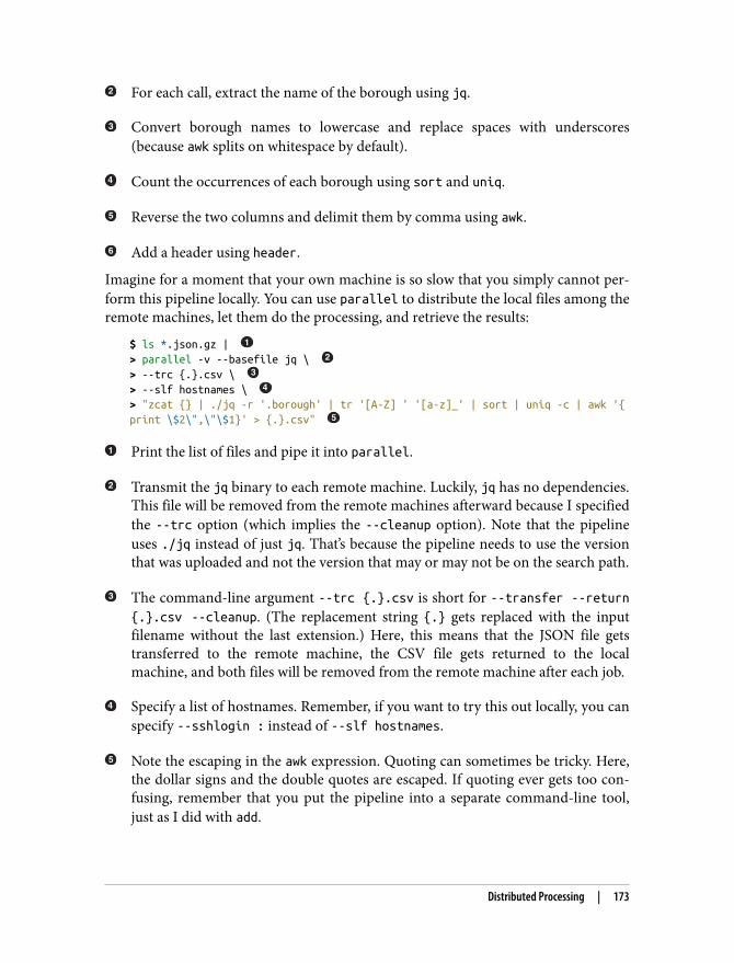
For each call, extract the name of the borough using jq.

Convert borough names to lowercase and replace spaces with underscores(because awk splits on whitespace by default).

Count the occurrences of each borough using sort and uniq.

Reverse the two columns and delimit them by comma using awk.

Add a header using header.

Imagine for a moment that your own machine is so slow that you simply cannot per‐form this pipeline locally. You can use parallel to distribute the local files among theremote machines, let them do the processing, and retrieve the results:

$ ls *.json.gz | > parallel -v --basefile jq \ > --trc {.}.csv \ > --slf hostnames \ > "zcat {} | ./jq -r '.borough' | tr '[A-Z] ' '[a-z]_' | sort | uniq -c | awk '{print \$2\",\"\$1}' > {.}.csv"

Print the list of files and pipe it into parallel.

Transmit the jq binary to each remote machine. Luckily, jq has no dependencies.This file will be removed from the remote machines afterward because I specifiedthe --trc option (which implies the --cleanup option). Note that the pipelineuses ./jq instead of just jq. That’s because the pipeline needs to use the versionthat was uploaded and not the version that may or may not be on the search path.

The command-line argument --trc {.}.csv is short for --transfer --return{.}.csv --cleanup. (The replacement string {.} gets replaced with the inputfilename without the last extension.) Here, this means that the JSON file getstransferred to the remote machine, the CSV file gets returned to the localmachine, and both files will be removed from the remote machine after each job.

Specify a list of hostnames. Remember, if you want to try this out locally, you canspecify --sshlogin : instead of --slf hostnames.

Note the escaping in the awk expression. Quoting can sometimes be tricky. Here,the dollar signs and the double quotes are escaped. If quoting ever gets too con‐fusing, remember that you put the pipeline into a separate command-line tool,just as I did with add.

Distributed Processing | 173

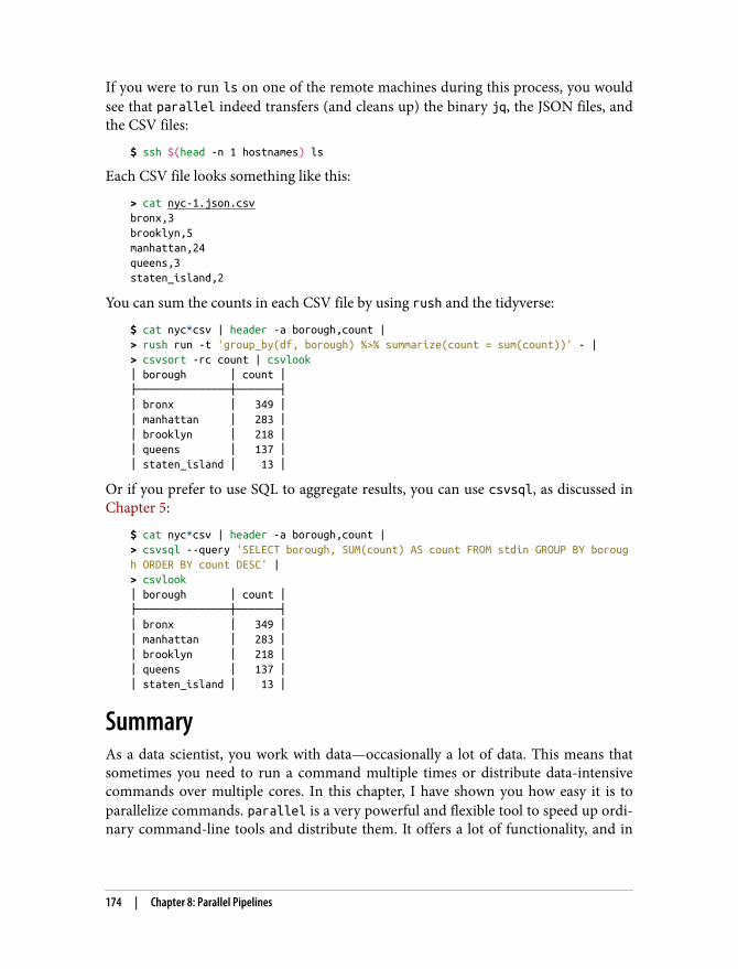
If you were to run ls on one of the remote machines during this process, you wouldsee that parallel indeed transfers (and cleans up) the binary jq, the JSON files, andthe CSV files:

$ ssh $(head -n 1 hostnames) ls

Each CSV file looks something like this:

> cat nyc-1.json.csvbronx,3brooklyn,5manhattan,24queens,3staten_island,2

You can sum the counts in each CSV file by using rush and the tidyverse:

$ cat nyc*csv | header -a borough,count |> rush run -t 'group_by(df, borough) %>% summarize(count = sum(count))' - |> csvsort -rc count | csvlook│ borough │ count │├───────────────┼───────┤│ bronx │ 349 ││ manhattan │ 283 ││ brooklyn │ 218 ││ queens │ 137 ││ staten_island │ 13 │

Or if you prefer to use SQL to aggregate results, you can use csvsql, as discussed inChapter 5:

$ cat nyc*csv | header -a borough,count |> csvsql --query 'SELECT borough, SUM(count) AS count FROM stdin GROUP BY borough ORDER BY count DESC' |> csvlook│ borough │ count │├───────────────┼───────┤│ bronx │ 349 ││ manhattan │ 283 ││ brooklyn │ 218 ││ queens │ 137 ││ staten_island │ 13 │

SummaryAs a data scientist, you work with data—occasionally a lot of data. This means thatsometimes you need to run a command multiple times or distribute data-intensivecommands over multiple cores. In this chapter, I have shown you how easy it is toparallelize commands. parallel is a very powerful and flexible tool to speed up ordi‐nary command-line tools and distribute them. It offers a lot of functionality, and in

174 | Chapter 8: Parallel Pipelines

this chapter I’ve only been able to scratch the surface. In the next chapter I’m going tocover the fourth step of the OSEMN model: modeling data.

For Further ExplorationOnce you have a basic understanding of parallel and its most important options, Irecommend that you take a look at its online tutorial. Among other things, you’lllearn different ways of specifying input, how to keep a log of all the jobs, and how totimeout, resume, and retry jobs. As Ole Tange, creator of parallel, says in this tuto‐rial, “Your command line will love you for it.”

For Further Exploration | 175

CHAPTER 9

Modeling Data

In this chapter we’re going to perform the fourth step of the OSEMN model: model‐ing data. Generally speaking, a model is an abstract or higher-level description ofyour data. Modeling is a bit like creating visualizations in the sense that we’re taking astep back from the individual data points to see the bigger picture.

Visualizations are characterized by shapes, positions, and colors: we can interpretthem by looking at them. Models, on the other hand, are internally characterized bynumbers, which means that computers can use them to do things like make predic‐tions about new data points. (We can still visualize models so that we can try tounderstand them and see how they are performing.)

In this chapter I’ll consider three types of algorithms commonly used to model data:

• Dimensionality reduction• Regression• Classification

These algorithms come from the field of statistics and machine learning, so I’m goingto change the vocabulary a bit. Let’s assume that I have a CSV file, also known as adataset. Each row, except for the header, is considered a data point. Each data pointhas one or more features, or properties that have been measured. Sometimes a datapoint also has a label, which is, generally speaking, a judgment or outcome. Thisbecomes more concrete when I introduce the wine dataset later in this chapter.

The first type of algorithm (dimensionality reduction) is most often unsupervised,which means that it creates a model based on the features of the dataset only. Theother two types of algorithms (regression and classification) are by definition super‐vised algorithms, which means that they also incorporate the labels into the model.

177

1 Sergey Lisitsyn, Christian Widmer, and Fernando J. Iglesias Garcia, tapkee – an Efficient Dimension ReductionLibrary, version 1.2, 2013, http://tapkee.lisitsyn.me.

2 John Langford, vw – Fast Machine Learning Library for Online Learning, version 8.10.1, 2021, https://vowpalwabbit.org.

3 Educational Testing Service, skll – SciKit-Learn Laboratory, version 2.5.0, 2021, https://skll.readthedocs.org.

This chapter is by no means an introduction to machine learning.That implies that I must skim over many details. My general adviceis that you become familiar with an algorithm before applying it toyour data. At the end of this chapter I recommend a few booksabout machine learning.

OverviewIn this chapter, you’ll learn how to:

• Reduce the dimensionality of your dataset using tapkee1

• Predict the quality of white wine using vw2

• Classify wine as red or white using skll3

This chapter starts with the following file:

$ cd /data/ch09 $ ltotal 4.0K-rw-r--r-- 1 dst dst 503 Jun 29 14:34 classify.cfg

The instructions for getting this file are in Chapter 2. Any other files are either down‐loaded or generated using command-line tools.

More Wine, Please!Throughout this chapter, I’ll be using a dataset of wine tasters’ notes on red and whitevarieties of a Portuguese wine called vinho verde. Each data point represents a wine.Each wine is rated on 11 physicochemical properties: (1) fixed acidity, (2) volatileacidity, (3) citric acid, (4) residual sugar, (5) chlorides, (6) free sulfur dioxide, (7) totalsulfur dioxide, (8) density, (9) pH, (10) sulfates, and (11) alcohol. There is also anoverall quality score between 0 (very bad) and 10 (excellent), which is the median ofat least three evaluations by wine experts. More information about this dataset isavailable at the UCI Machine Learning Repository.

178 | Chapter 9: Modeling Data

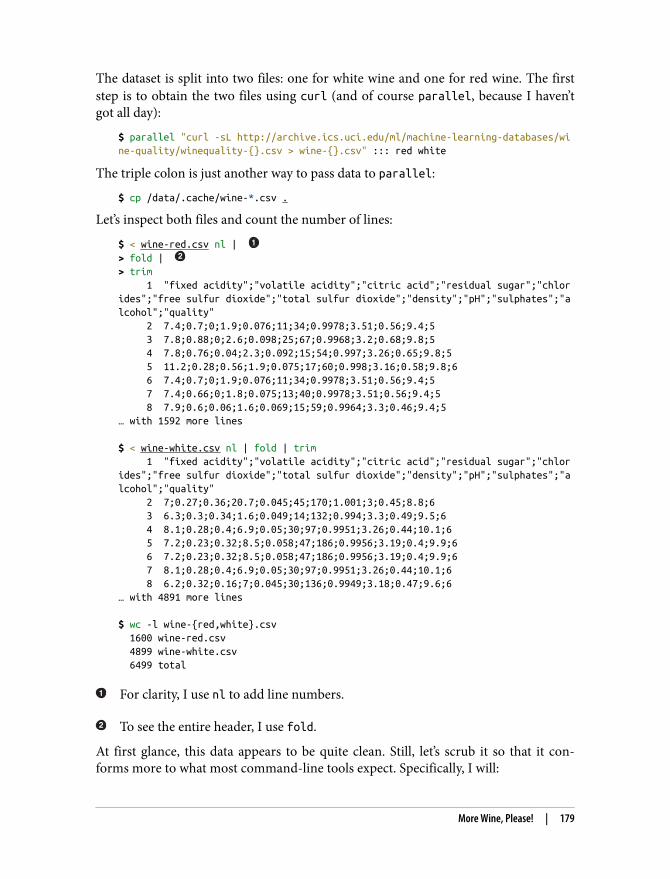
The dataset is split into two files: one for white wine and one for red wine. The firststep is to obtain the two files using curl (and of course parallel, because I haven’tgot all day):

$ parallel "curl -sL http://archive.ics.uci.edu/ml/machine-learning-databases/wine-quality/winequality-{}.csv > wine-{}.csv" ::: red white

The triple colon is just another way to pass data to parallel:

$ cp /data/.cache/wine-*.csv .

Let’s inspect both files and count the number of lines:

$ < wine-red.csv nl | > fold | > trim 1 "fixed acidity";"volatile acidity";"citric acid";"residual sugar";"chlorides";"free sulfur dioxide";"total sulfur dioxide";"density";"pH";"sulphates";"alcohol";"quality" 2 7.4;0.7;0;1.9;0.076;11;34;0.9978;3.51;0.56;9.4;5 3 7.8;0.88;0;2.6;0.098;25;67;0.9968;3.2;0.68;9.8;5 4 7.8;0.76;0.04;2.3;0.092;15;54;0.997;3.26;0.65;9.8;5 5 11.2;0.28;0.56;1.9;0.075;17;60;0.998;3.16;0.58;9.8;6 6 7.4;0.7;0;1.9;0.076;11;34;0.9978;3.51;0.56;9.4;5 7 7.4;0.66;0;1.8;0.075;13;40;0.9978;3.51;0.56;9.4;5 8 7.9;0.6;0.06;1.6;0.069;15;59;0.9964;3.3;0.46;9.4;5… with 1592 more lines $ < wine-white.csv nl | fold | trim 1 "fixed acidity";"volatile acidity";"citric acid";"residual sugar";"chlorides";"free sulfur dioxide";"total sulfur dioxide";"density";"pH";"sulphates";"alcohol";"quality" 2 7;0.27;0.36;20.7;0.045;45;170;1.001;3;0.45;8.8;6 3 6.3;0.3;0.34;1.6;0.049;14;132;0.994;3.3;0.49;9.5;6 4 8.1;0.28;0.4;6.9;0.05;30;97;0.9951;3.26;0.44;10.1;6 5 7.2;0.23;0.32;8.5;0.058;47;186;0.9956;3.19;0.4;9.9;6 6 7.2;0.23;0.32;8.5;0.058;47;186;0.9956;3.19;0.4;9.9;6 7 8.1;0.28;0.4;6.9;0.05;30;97;0.9951;3.26;0.44;10.1;6 8 6.2;0.32;0.16;7;0.045;30;136;0.9949;3.18;0.47;9.6;6… with 4891 more lines $ wc -l wine-{red,white}.csv 1600 wine-red.csv 4899 wine-white.csv 6499 total

For clarity, I use nl to add line numbers.

To see the entire header, I use fold.

At first glance, this data appears to be quite clean. Still, let’s scrub it so that it con‐forms more to what most command-line tools expect. Specifically, I will:

More Wine, Please! | 179

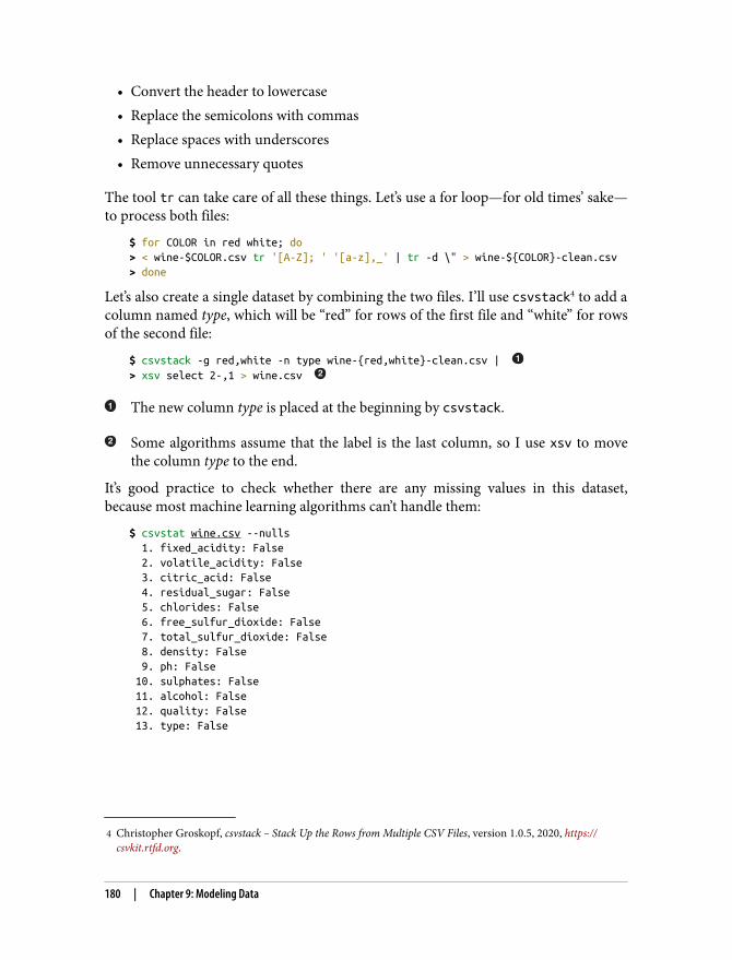
4 Christopher Groskopf, csvstack – Stack Up the Rows from Multiple CSV Files, version 1.0.5, 2020, https://csvkit.rtfd.org.

• Convert the header to lowercase• Replace the semicolons with commas• Replace spaces with underscores• Remove unnecessary quotes

The tool tr can take care of all these things. Let’s use a for loop—for old times’ sake—to process both files:

$ for COLOR in red white; do> < wine-$COLOR.csv tr '[A-Z]; ' '[a-z],_' | tr -d \" > wine-${COLOR}-clean.csv> done

Let’s also create a single dataset by combining the two files. I’ll use csvstack4 to add acolumn named type, which will be “red” for rows of the first file and “white” for rowsof the second file:

$ csvstack -g red,white -n type wine-{red,white}-clean.csv | > xsv select 2-,1 > wine.csv

The new column type is placed at the beginning by csvstack.

Some algorithms assume that the label is the last column, so I use xsv to movethe column type to the end.

It’s good practice to check whether there are any missing values in this dataset,because most machine learning algorithms can’t handle them:

$ csvstat wine.csv --nulls 1. fixed_acidity: False 2. volatile_acidity: False 3. citric_acid: False 4. residual_sugar: False 5. chlorides: False 6. free_sulfur_dioxide: False 7. total_sulfur_dioxide: False 8. density: False 9. ph: False 10. sulphates: False 11. alcohol: False 12. quality: False 13. type: False

180 | Chapter 9: Modeling Data

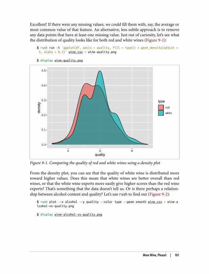
Excellent! If there were any missing values, we could fill them with, say, the average ormost common value of that feature. An alternative, less subtle approach is to removeany data points that have at least one missing value. Just out of curiosity, let’s see whatthe distribution of quality looks like for both red and white wines (Figure 9-1):

$ rush run -t 'ggplot(df, aes(x = quality, fill = type)) + geom_density(adjust = 3, alpha = 0.5)' wine.csv > wine-quality.png $ display wine-quality.png

Figure 9-1. Comparing the quality of red and white wines using a density plot

From the density plot, you can see that the quality of white wine is distributed moretoward higher values. Does this mean that white wines are better overall than redwines, or that the white wine experts more easily give higher scores than the red wineexperts? That’s something that the data doesn’t tell us. Or is there perhaps a relation‐ship between alcohol content and quality? Let’s use rush to find out (Figure 9-2):

$ rush plot --x alcohol --y quality --color type --geom smooth wine.csv > wine-alcohol-vs-quality.png $ display wine-alcohol-vs-quality.png

More Wine, Please! | 181

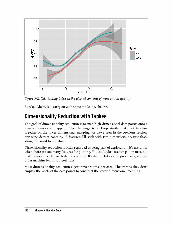
Figure 9-2. Relationship between the alcohol contents of wine and its quality

Eureka! Ahem, let’s carry on with some modeling, shall we?

Dimensionality Reduction with TapkeeThe goal of dimensionality reduction is to map high-dimensional data points onto alower-dimensional mapping. The challenge is to keep similar data points closetogether on the lower-dimensional mapping. As we’ve seen in the previous section,our wine dataset contains 13 features. I’ll stick with two dimensions because that’sstraightforward to visualize.

Dimensionality reduction is often regarded as being part of exploration. It’s useful forwhen there are too many features for plotting. You could do a scatter-plot matrix, butthat shows you only two features at a time. It’s also useful as a preprocessing step forother machine learning algorithms.

Most dimensionality reduction algorithms are unsupervised. This means they don’temploy the labels of the data points to construct the lower-dimensional mapping.

182 | Chapter 9: Modeling Data

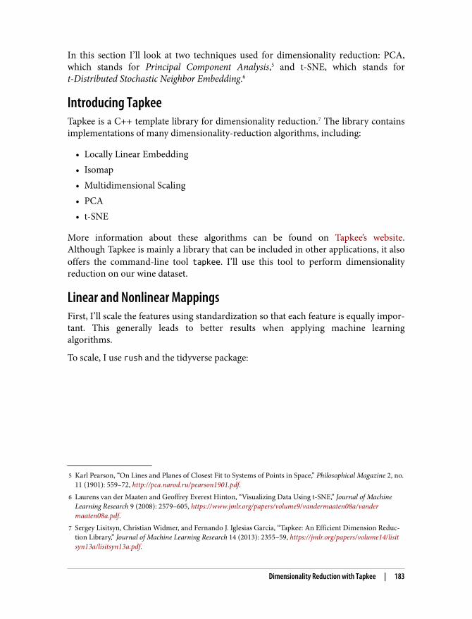
5 Karl Pearson, “On Lines and Planes of Closest Fit to Systems of Points in Space,” Philosophical Magazine 2, no.11 (1901): 559–72, http://pca.narod.ru/pearson1901.pdf.

6 Laurens van der Maaten and Geoffrey Everest Hinton, “Visualizing Data Using t-SNE,” Journal of MachineLearning Research 9 (2008): 2579–605, https://www.jmlr.org/papers/volume9/vandermaaten08a/vandermaaten08a.pdf.

7 Sergey Lisitsyn, Christian Widmer, and Fernando J. Iglesias Garcia, “Tapkee: An Efficient Dimension Reduc‐tion Library,” Journal of Machine Learning Research 14 (2013): 2355–59, https://jmlr.org/papers/volume14/lisitsyn13a/lisitsyn13a.pdf.

In this section I’ll look at two techniques used for dimensionality reduction: PCA,which stands for Principal Component Analysis,5 and t-SNE, which stands fort-Distributed Stochastic Neighbor Embedding.6

Introducing TapkeeTapkee is a C++ template library for dimensionality reduction.7 The library containsimplementations of many dimensionality-reduction algorithms, including:

• Locally Linear Embedding• Isomap• Multidimensional Scaling• PCA• t-SNE

More information about these algorithms can be found on Tapkee’s website.Although Tapkee is mainly a library that can be included in other applications, it alsooffers the command-line tool tapkee. I’ll use this tool to perform dimensionalityreduction on our wine dataset.

Linear and Nonlinear MappingsFirst, I’ll scale the features using standardization so that each feature is equally impor‐tant. This generally leads to better results when applying machine learningalgorithms.

To scale, I use rush and the tidyverse package:

Dimensionality Reduction with Tapkee | 183

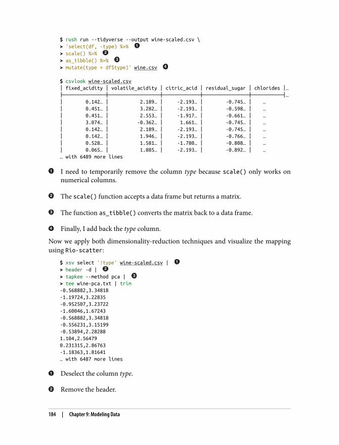
$ rush run --tidyverse --output wine-scaled.csv \> 'select(df, -type) %>% > scale() %>% > as_tibble() %>% > mutate(type = df$type)' wine.csv $ csvlook wine-scaled.csv│ fixed_acidity │ volatile_acidity │ citric_acid │ residual_sugar │ chlorides │…├───────────────┼──────────────────┼─────────────┼────────────────┼───────────┤…│ 0.142… │ 2.189… │ -2.193… │ -0.745… │ …│ 0.451… │ 3.282… │ -2.193… │ -0.598… │ …│ 0.451… │ 2.553… │ -1.917… │ -0.661… │ …│ 3.074… │ -0.362… │ 1.661… │ -0.745… │ …│ 0.142… │ 2.189… │ -2.193… │ -0.745… │ …│ 0.142… │ 1.946… │ -2.193… │ -0.766… │ …│ 0.528… │ 1.581… │ -1.780… │ -0.808… │ …│ 0.065… │ 1.885… │ -2.193… │ -0.892… │ …… with 6489 more lines

I need to temporarily remove the column type because scale() only works onnumerical columns.

The scale() function accepts a data frame but returns a matrix.

The function as_tibble() converts the matrix back to a data frame.

Finally, I add back the type column.

Now we apply both dimensionality-reduction techniques and visualize the mappingusing Rio-scatter:

$ xsv select '!type' wine-scaled.csv | > header -d | > tapkee --method pca | > tee wine-pca.txt | trim-0.568882,3.34818-1.19724,3.22835-0.952507,3.23722-1.60046,1.67243-0.568882,3.34818-0.556231,3.15199-0.53894,2.282881.104,2.564790.231315,2.86763-1.18363,1.81641… with 6487 more lines

Deselect the column type.

Remove the header.

184 | Chapter 9: Modeling Data

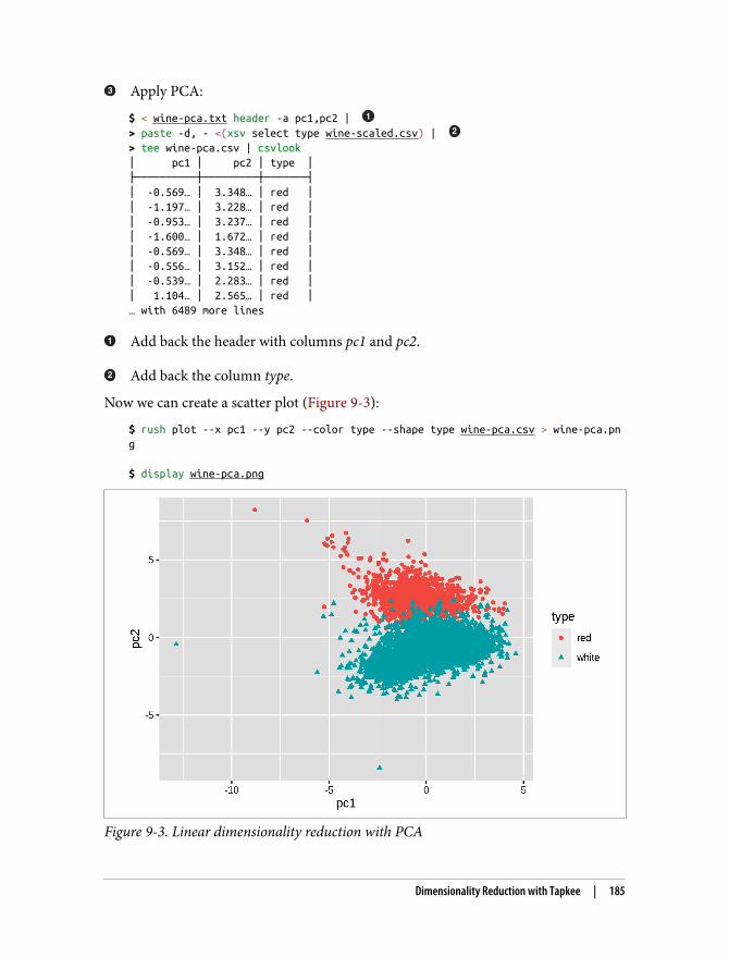
Apply PCA:

$ < wine-pca.txt header -a pc1,pc2 | > paste -d, - <(xsv select type wine-scaled.csv) | > tee wine-pca.csv | csvlook│ pc1 │ pc2 │ type │├──────────┼─────────┼───────┤│ -0.569… │ 3.348… │ red ││ -1.197… │ 3.228… │ red ││ -0.953… │ 3.237… │ red ││ -1.600… │ 1.672… │ red ││ -0.569… │ 3.348… │ red ││ -0.556… │ 3.152… │ red ││ -0.539… │ 2.283… │ red ││ 1.104… │ 2.565… │ red │… with 6489 more lines

Add back the header with columns pc1 and pc2.

Add back the column type.

Now we can create a scatter plot (Figure 9-3):

$ rush plot --x pc1 --y pc2 --color type --shape type wine-pca.csv > wine-pca.png $ display wine-pca.png

Figure 9-3. Linear dimensionality reduction with PCA

Dimensionality Reduction with Tapkee | 185

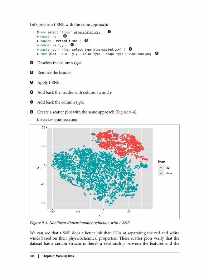
Let’s perform t-SNE with the same approach:

$ xsv select '!type' wine-scaled.csv | > header -d | > tapkee --method t-sne | > header -a x,y | > paste -d, - <(xsv select type wine-scaled.csv) | > rush plot --x x --y y --color type --shape type > wine-tsne.png

Deselect the column type.

Remove the header.

Apply t-SNE.

Add back the header with columns x and y.

Add back the column type.

Create a scatter plot with the same approach (Figure 9-4):

$ display wine-tsne.png

Figure 9-4. Nonlinear dimensionality reduction with t-SNE

We can see that t-SNE does a better job than PCA at separating the red and whitewines based on their physicochemical properties. These scatter plots verify that thedataset has a certain structure; there’s a relationship between the features and the

186 | Chapter 9: Modeling Data

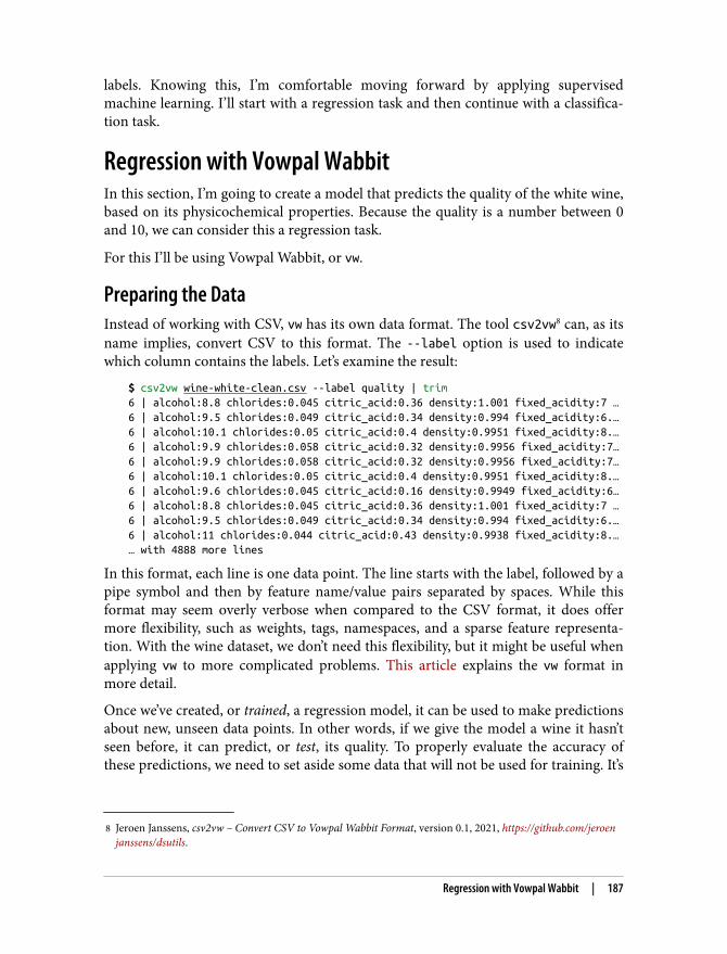
8 Jeroen Janssens, csv2vw – Convert CSV to Vowpal Wabbit Format, version 0.1, 2021, https://github.com/jeroenjanssens/dsutils.

labels. Knowing this, I’m comfortable moving forward by applying supervisedmachine learning. I’ll start with a regression task and then continue with a classifica‐tion task.

Regression with Vowpal WabbitIn this section, I’m going to create a model that predicts the quality of the white wine,based on its physicochemical properties. Because the quality is a number between 0and 10, we can consider this a regression task.

For this I’ll be using Vowpal Wabbit, or vw.

Preparing the DataInstead of working with CSV, vw has its own data format. The tool csv2vw8 can, as itsname implies, convert CSV to this format. The --label option is used to indicatewhich column contains the labels. Let’s examine the result:

$ csv2vw wine-white-clean.csv --label quality | trim6 | alcohol:8.8 chlorides:0.045 citric_acid:0.36 density:1.001 fixed_acidity:7 …6 | alcohol:9.5 chlorides:0.049 citric_acid:0.34 density:0.994 fixed_acidity:6.…6 | alcohol:10.1 chlorides:0.05 citric_acid:0.4 density:0.9951 fixed_acidity:8.…6 | alcohol:9.9 chlorides:0.058 citric_acid:0.32 density:0.9956 fixed_acidity:7…6 | alcohol:9.9 chlorides:0.058 citric_acid:0.32 density:0.9956 fixed_acidity:7…6 | alcohol:10.1 chlorides:0.05 citric_acid:0.4 density:0.9951 fixed_acidity:8.…6 | alcohol:9.6 chlorides:0.045 citric_acid:0.16 density:0.9949 fixed_acidity:6…6 | alcohol:8.8 chlorides:0.045 citric_acid:0.36 density:1.001 fixed_acidity:7 …6 | alcohol:9.5 chlorides:0.049 citric_acid:0.34 density:0.994 fixed_acidity:6.…6 | alcohol:11 chlorides:0.044 citric_acid:0.43 density:0.9938 fixed_acidity:8.…… with 4888 more lines

In this format, each line is one data point. The line starts with the label, followed by apipe symbol and then by feature name/value pairs separated by spaces. While thisformat may seem overly verbose when compared to the CSV format, it does offermore flexibility, such as weights, tags, namespaces, and a sparse feature representa‐tion. With the wine dataset, we don’t need this flexibility, but it might be useful whenapplying vw to more complicated problems. This article explains the vw format inmore detail.

Once we’ve created, or trained, a regression model, it can be used to make predictionsabout new, unseen data points. In other words, if we give the model a wine it hasn’tseen before, it can predict, or test, its quality. To properly evaluate the accuracy ofthese predictions, we need to set aside some data that will not be used for training. It’s

Regression with Vowpal Wabbit | 187

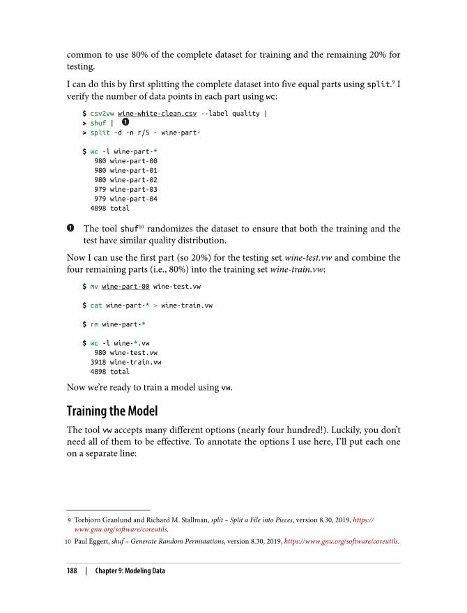
9 Torbjorn Granlund and Richard M. Stallman, split – Split a File into Pieces, version 8.30, 2019, https://www.gnu.org/software/coreutils.

10 Paul Eggert, shuf – Generate Random Permutations, version 8.30, 2019, https://www.gnu.org/software/coreutils.

common to use 80% of the complete dataset for training and the remaining 20% fortesting.

I can do this by first splitting the complete dataset into five equal parts using split.9 Iverify the number of data points in each part using wc:

$ csv2vw wine-white-clean.csv --label quality |> shuf | > split -d -n r/5 - wine-part- $ wc -l wine-part-* 980 wine-part-00 980 wine-part-01 980 wine-part-02 979 wine-part-03 979 wine-part-04 4898 total

The tool shuf10 randomizes the dataset to ensure that both the training and thetest have similar quality distribution.

Now I can use the first part (so 20%) for the testing set wine-test.vw and combine thefour remaining parts (i.e., 80%) into the training set wine-train.vw:

$ mv wine-part-00 wine-test.vw $ cat wine-part-* > wine-train.vw $ rm wine-part-* $ wc -l wine-*.vw 980 wine-test.vw 3918 wine-train.vw 4898 total

Now we’re ready to train a model using vw.

Training the ModelThe tool vw accepts many different options (nearly four hundred!). Luckily, you don’tneed all of them to be effective. To annotate the options I use here, I’ll put each oneon a separate line:

188 | Chapter 9: Modeling Data

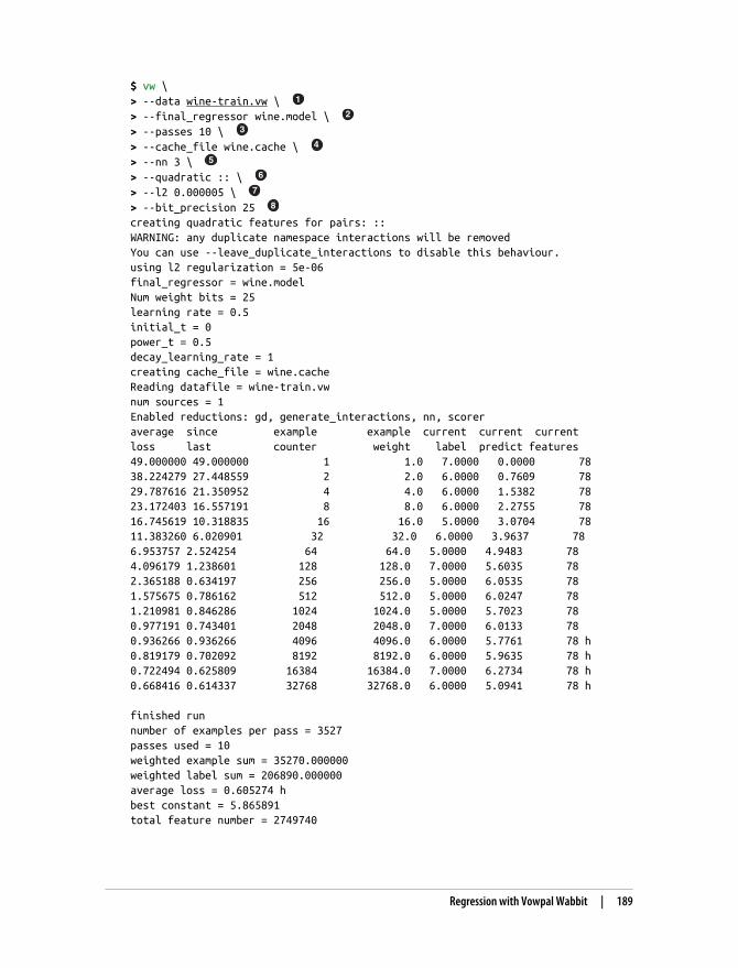
$ vw \> --data wine-train.vw \ > --final_regressor wine.model \ > --passes 10 \ > --cache_file wine.cache \ > --nn 3 \ > --quadratic :: \ > --l2 0.000005 \ > --bit_precision 25 creating quadratic features for pairs: ::WARNING: any duplicate namespace interactions will be removedYou can use --leave_duplicate_interactions to disable this behaviour.using l2 regularization = 5e-06final_regressor = wine.modelNum weight bits = 25learning rate = 0.5initial_t = 0power_t = 0.5decay_learning_rate = 1creating cache_file = wine.cacheReading datafile = wine-train.vwnum sources = 1Enabled reductions: gd, generate_interactions, nn, scoreraverage since example example current current currentloss last counter weight label predict features49.000000 49.000000 1 1.0 7.0000 0.0000 7838.224279 27.448559 2 2.0 6.0000 0.7609 7829.787616 21.350952 4 4.0 6.0000 1.5382 7823.172403 16.557191 8 8.0 6.0000 2.2755 7816.745619 10.318835 16 16.0 5.0000 3.0704 7811.383260 6.020901 32 32.0 6.0000 3.9637 786.953757 2.524254 64 64.0 5.0000 4.9483 784.096179 1.238601 128 128.0 7.0000 5.6035 782.365188 0.634197 256 256.0 5.0000 6.0535 781.575675 0.786162 512 512.0 5.0000 6.0247 781.210981 0.846286 1024 1024.0 5.0000 5.7023 780.977191 0.743401 2048 2048.0 7.0000 6.0133 780.936266 0.936266 4096 4096.0 6.0000 5.7761 78 h0.819179 0.702092 8192 8192.0 6.0000 5.9635 78 h0.722494 0.625809 16384 16384.0 7.0000 6.2734 78 h0.668416 0.614337 32768 32768.0 6.0000 5.0941 78 h finished runnumber of examples per pass = 3527passes used = 10weighted example sum = 35270.000000weighted label sum = 206890.000000average loss = 0.605274 hbest constant = 5.865891total feature number = 2749740

Regression with Vowpal Wabbit | 189

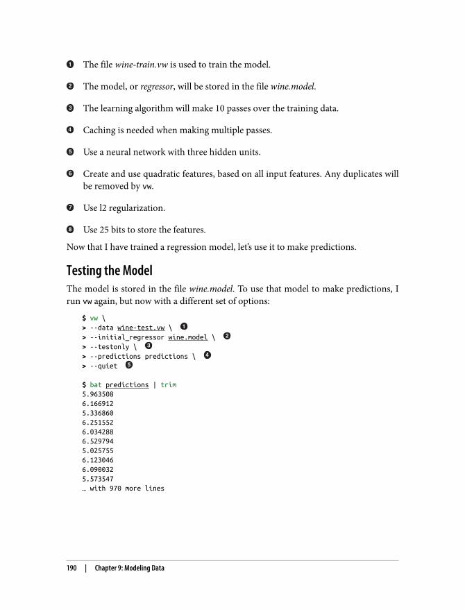
The file wine-train.vw is used to train the model.

The model, or regressor, will be stored in the file wine.model.

The learning algorithm will make 10 passes over the training data.

Caching is needed when making multiple passes.

Use a neural network with three hidden units.

Create and use quadratic features, based on all input features. Any duplicates willbe removed by vw.

Use l2 regularization.

Use 25 bits to store the features.

Now that I have trained a regression model, let’s use it to make predictions.

Testing the ModelThe model is stored in the file wine.model. To use that model to make predictions, Irun vw again, but now with a different set of options:

$ vw \> --data wine-test.vw \ > --initial_regressor wine.model \ > --testonly \ > --predictions predictions \ > --quiet $ bat predictions | trim5.9635086.1669125.3368606.2515526.0342886.5297945.0257556.1230466.0900325.573547… with 970 more lines

190 | Chapter 9: Modeling Data

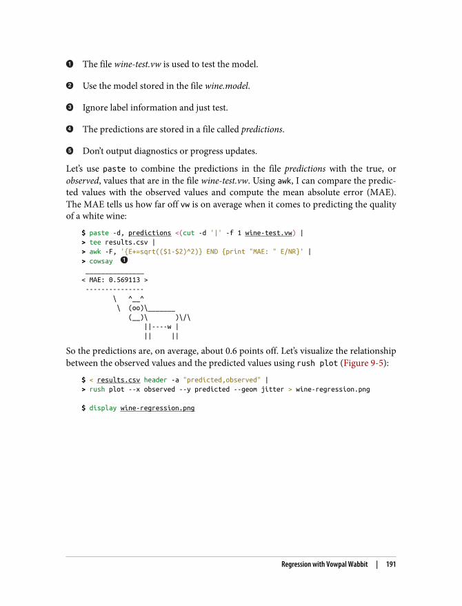
The file wine-test.vw is used to test the model.

Use the model stored in the file wine.model.

Ignore label information and just test.

The predictions are stored in a file called predictions.

Don’t output diagnostics or progress updates.

Let’s use paste to combine the predictions in the file predictions with the true, orobserved, values that are in the file wine-test.vw. Using awk, I can compare the predic‐ted values with the observed values and compute the mean absolute error (MAE).The MAE tells us how far off vw is on average when it comes to predicting the qualityof a white wine:

$ paste -d, predictions <(cut -d '|' -f 1 wine-test.vw) |> tee results.csv |> awk -F, '{E+=sqrt(($1-$2)^2)} END {print "MAE: " E/NR}' |> cowsay _______________< MAE: 0.569113 > --------------- \ ^__^ \ (oo)\_______ (__)\ )\/\ ||----w | || ||

So the predictions are, on average, about 0.6 points off. Let’s visualize the relationshipbetween the observed values and the predicted values using rush plot (Figure 9-5):

$ < results.csv header -a "predicted,observed" |> rush plot --x observed --y predicted --geom jitter > wine-regression.png $ display wine-regression.png

Regression with Vowpal Wabbit | 191

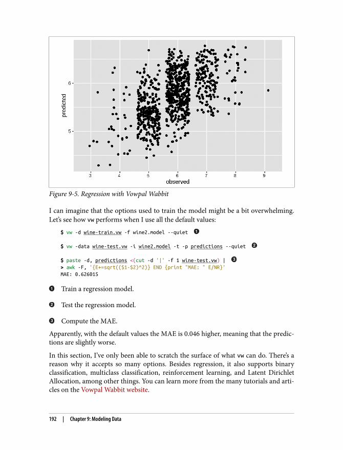
Figure 9-5. Regression with Vowpal Wabbit

I can imagine that the options used to train the model might be a bit overwhelming.Let’s see how vw performs when I use all the default values:

$ vw -d wine-train.vw -f wine2.model --quiet $ vw -data wine-test.vw -i wine2.model -t -p predictions --quiet $ paste -d, predictions <(cut -d '|' -f 1 wine-test.vw) | > awk -F, '{E+=sqrt(($1-$2)^2)} END {print "MAE: " E/NR}'MAE: 0.626015

Train a regression model.

Test the regression model.

Compute the MAE.

Apparently, with the default values the MAE is 0.046 higher, meaning that the predic‐tions are slightly worse.

In this section, I’ve only been able to scratch the surface of what vw can do. There’s areason why it accepts so many options. Besides regression, it also supports binaryclassification, multiclass classification, reinforcement learning, and Latent DirichletAllocation, among other things. You can learn more from the many tutorials and arti‐cles on the Vowpal Wabbit website.

192 | Chapter 9: Modeling Data

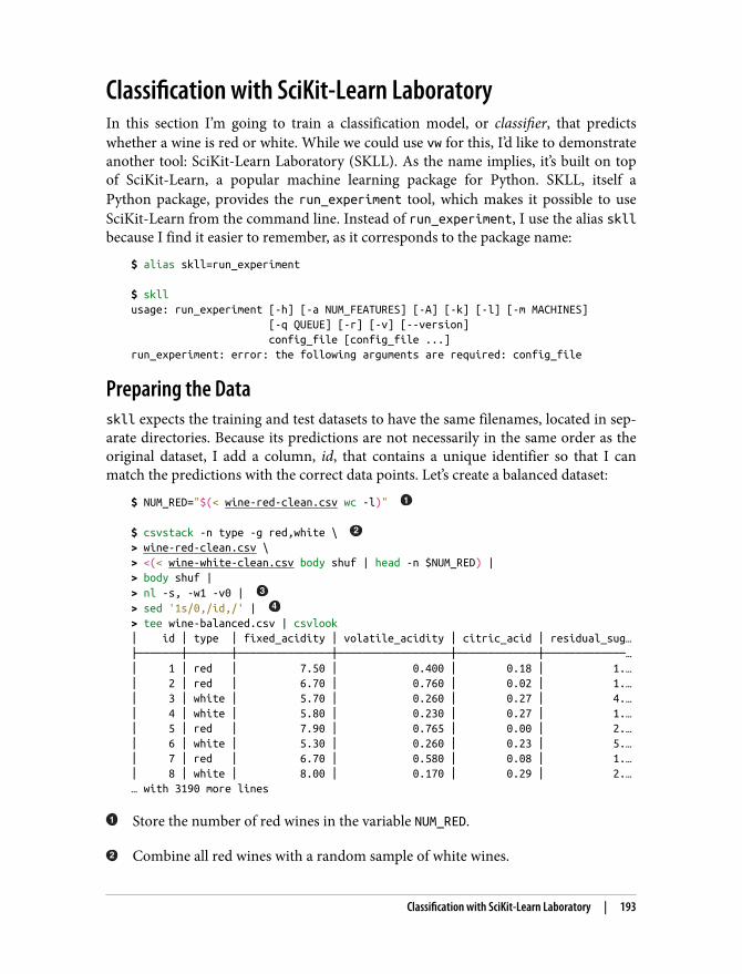
Classification with SciKit-Learn LaboratoryIn this section I’m going to train a classification model, or classifier, that predictswhether a wine is red or white. While we could use vw for this, I’d like to demonstrateanother tool: SciKit-Learn Laboratory (SKLL). As the name implies, it’s built on topof SciKit-Learn, a popular machine learning package for Python. SKLL, itself aPython package, provides the run_experiment tool, which makes it possible to useSciKit-Learn from the command line. Instead of run_experiment, I use the alias skllbecause I find it easier to remember, as it corresponds to the package name:

$ alias skll=run_experiment $ skllusage: run_experiment [-h] [-a NUM_FEATURES] [-A] [-k] [-l] [-m MACHINES] [-q QUEUE] [-r] [-v] [--version] config_file [config_file ...]run_experiment: error: the following arguments are required: config_file

Preparing the Dataskll expects the training and test datasets to have the same filenames, located in sep‐arate directories. Because its predictions are not necessarily in the same order as theoriginal dataset, I add a column, id, that contains a unique identifier so that I canmatch the predictions with the correct data points. Let’s create a balanced dataset:

$ NUM_RED="$(< wine-red-clean.csv wc -l)" $ csvstack -n type -g red,white \ > wine-red-clean.csv \> <(< wine-white-clean.csv body shuf | head -n $NUM_RED) |> body shuf |> nl -s, -w1 -v0 | > sed '1s/0,/id,/' | > tee wine-balanced.csv | csvlook│ id │ type │ fixed_acidity │ volatile_acidity │ citric_acid │ residual_sug…├───────┼───────┼───────────────┼──────────────────┼─────────────┼─────────────…│ 1 │ red │ 7.50 │ 0.400 │ 0.18 │ 1.…│ 2 │ red │ 6.70 │ 0.760 │ 0.02 │ 1.…│ 3 │ white │ 5.70 │ 0.260 │ 0.27 │ 4.…│ 4 │ white │ 5.80 │ 0.230 │ 0.27 │ 1.…│ 5 │ red │ 7.90 │ 0.765 │ 0.00 │ 2.…│ 6 │ white │ 5.30 │ 0.260 │ 0.23 │ 5.…│ 7 │ red │ 6.70 │ 0.580 │ 0.08 │ 1.…│ 8 │ white │ 8.00 │ 0.170 │ 0.29 │ 2.…… with 3190 more lines

Store the number of red wines in the variable NUM_RED.

Combine all red wines with a random sample of white wines.

Classification with SciKit-Learn Laboratory | 193

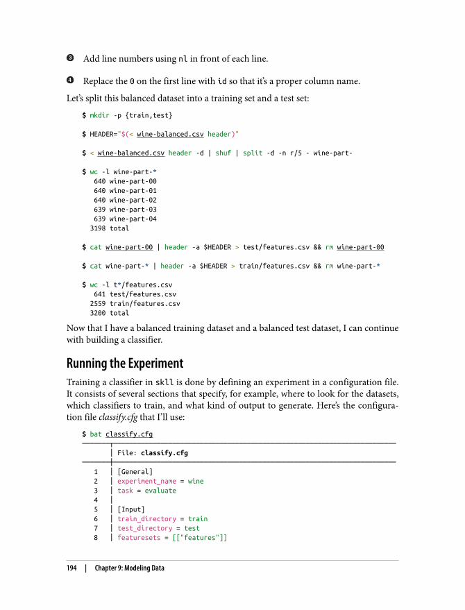
Add line numbers using nl in front of each line.

Replace the 0 on the first line with id so that it’s a proper column name.

Let’s split this balanced dataset into a training set and a test set:

$ mkdir -p {train,test} $ HEADER="$(< wine-balanced.csv header)"

$ < wine-balanced.csv header -d | shuf | split -d -n r/5 - wine-part- $ wc -l wine-part-* 640 wine-part-00 640 wine-part-01 640 wine-part-02 639 wine-part-03 639 wine-part-04 3198 total $ cat wine-part-00 | header -a $HEADER > test/features.csv && rm wine-part-00 $ cat wine-part-* | header -a $HEADER > train/features.csv && rm wine-part-* $ wc -l t*/features.csv 641 test/features.csv 2559 train/features.csv 3200 total

Now that I have a balanced training dataset and a balanced test dataset, I can continuewith building a classifier.

Running the ExperimentTraining a classifier in skll is done by defining an experiment in a configuration file.It consists of several sections that specify, for example, where to look for the datasets,which classifiers to train, and what kind of output to generate. Here’s the configura‐tion file classify.cfg that I’ll use:

$ bat classify.cfg───────┬──────────────────────────────────────────────────────────────────────── │ File: classify.cfg───────┼──────────────────────────────────────────────────────────────────────── 1 │ [General] 2 │ experiment_name = wine 3 │ task = evaluate 4 │ 5 │ [Input] 6 │ train_directory = train 7 │ test_directory = test 8 │ featuresets = [["features"]]

194 | Chapter 9: Modeling Data

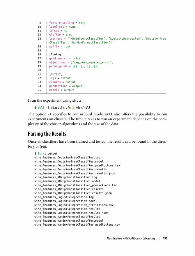
9 │ feature_scaling = both 10 │ label_col = type 11 │ id_col = id 12 │ shuffle = true 13 │ learners = ["KNeighborsClassifier", "LogisticRegression", "DecisionTree │ Classifier", "RandomForestClassifier"] 14 │ suffix = .csv 15 │ 16 │ [Tuning] 17 │ grid_search = false 18 │ objectives = ["neg_mean_squared_error"] 19 │ param_grids = [{}, {}, {}, {}] 20 │ 21 │ [Output] 22 │ logs = output 23 │ results = output 24 │ predictions = output 25 │ models = output───────┴────────────────────────────────────────────────────────────────────────

I run the experiment using skll:

$ skll -l classify.cfg 2>/dev/null

The option -l specifies to run in local mode. skll also offers the possibility to runexperiments on clusters. The time it takes to run an experiment depends on the com‐plexity of the chosen algorithms and the size of the data.

Parsing the ResultsOnce all classifiers have been trained and tested, the results can be found in the direc‐tory output:

$ ls -1 outputwine_features_DecisionTreeClassifier.logwine_features_DecisionTreeClassifier.modelwine_features_DecisionTreeClassifier_predictions.tsvwine_features_DecisionTreeClassifier.resultswine_features_DecisionTreeClassifier.results.jsonwine_features_KNeighborsClassifier.logwine_features_KNeighborsClassifier.modelwine_features_KNeighborsClassifier_predictions.tsvwine_features_KNeighborsClassifier.resultswine_features_KNeighborsClassifier.results.jsonwine_features_LogisticRegression.logwine_features_LogisticRegression.modelwine_features_LogisticRegression_predictions.tsvwine_features_LogisticRegression.resultswine_features_LogisticRegression.results.jsonwine_features_RandomForestClassifier.logwine_features_RandomForestClassifier.modelwine_features_RandomForestClassifier_predictions.tsv

Classification with SciKit-Learn Laboratory | 195

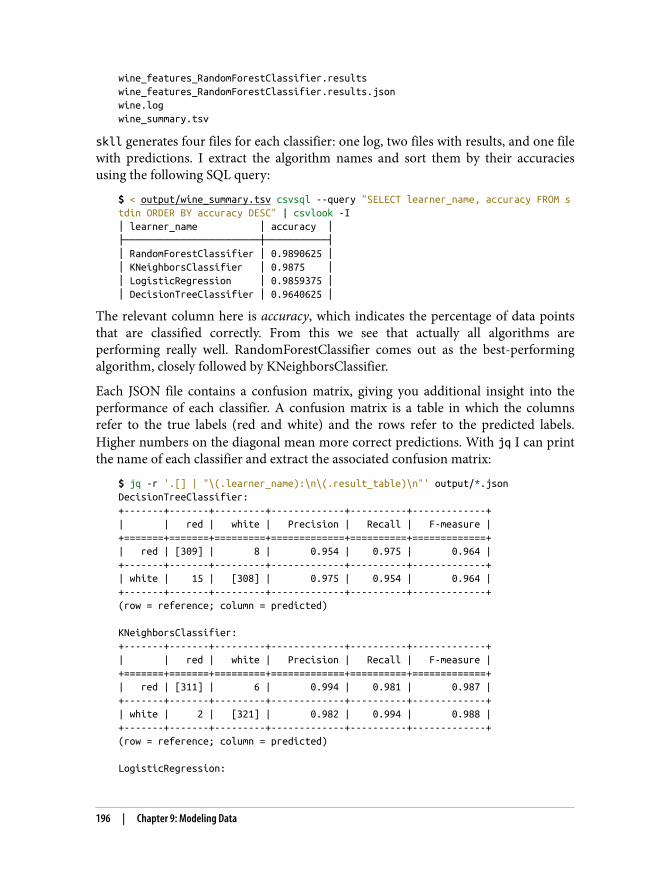
wine_features_RandomForestClassifier.resultswine_features_RandomForestClassifier.results.jsonwine.logwine_summary.tsv

skll generates four files for each classifier: one log, two files with results, and one filewith predictions. I extract the algorithm names and sort them by their accuraciesusing the following SQL query:

$ < output/wine_summary.tsv csvsql --query "SELECT learner_name, accuracy FROM stdin ORDER BY accuracy DESC" | csvlook -I│ learner_name │ accuracy │├────────────────────────┼───────────┤│ RandomForestClassifier │ 0.9890625 ││ KNeighborsClassifier │ 0.9875 ││ LogisticRegression │ 0.9859375 ││ DecisionTreeClassifier │ 0.9640625 │

The relevant column here is accuracy, which indicates the percentage of data pointsthat are classified correctly. From this we see that actually all algorithms areperforming really well. RandomForestClassifier comes out as the best-performingalgorithm, closely followed by KNeighborsClassifier.

Each JSON file contains a confusion matrix, giving you additional insight into theperformance of each classifier. A confusion matrix is a table in which the columnsrefer to the true labels (red and white) and the rows refer to the predicted labels.Higher numbers on the diagonal mean more correct predictions. With jq I can printthe name of each classifier and extract the associated confusion matrix:

$ jq -r '.[] | "\(.learner_name):\n\(.result_table)\n"' output/*.jsonDecisionTreeClassifier:+-------+-------+---------+-------------+----------+-------------+| | red | white | Precision | Recall | F-measure |+=======+=======+=========+=============+==========+=============+| red | [309] | 8 | 0.954 | 0.975 | 0.964 |+-------+-------+---------+-------------+----------+-------------+| white | 15 | [308] | 0.975 | 0.954 | 0.964 |+-------+-------+---------+-------------+----------+-------------+(row = reference; column = predicted) KNeighborsClassifier:+-------+-------+---------+-------------+----------+-------------+| | red | white | Precision | Recall | F-measure |+=======+=======+=========+=============+==========+=============+| red | [311] | 6 | 0.994 | 0.981 | 0.987 |+-------+-------+---------+-------------+----------+-------------+| white | 2 | [321] | 0.982 | 0.994 | 0.988 |+-------+-------+---------+-------------+----------+-------------+(row = reference; column = predicted) LogisticRegression:

196 | Chapter 9: Modeling Data

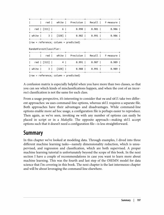
+-------+-------+---------+-------------+----------+-------------+| | red | white | Precision | Recall | F-measure |+=======+=======+=========+=============+==========+=============+| red | [311] | 6 | 0.990 | 0.981 | 0.986 |+-------+-------+---------+-------------+----------+-------------+| white | 3 | [320] | 0.982 | 0.991 | 0.986 |+-------+-------+---------+-------------+----------+-------------+(row = reference; column = predicted) RandomForestClassifier:+-------+-------+---------+-------------+----------+-------------+| | red | white | Precision | Recall | F-measure |+=======+=======+=========+=============+==========+=============+| red | [313] | 4 | 0.991 | 0.987 | 0.989 |+-------+-------+---------+-------------+----------+-------------+| white | 3 | [320] | 0.988 | 0.991 | 0.989 |+-------+-------+---------+-------------+----------+-------------+(row = reference; column = predicted)

A confusion matrix is especially helpful when you have more than two classes, so thatyou can see which kinds of misclassifications happen, and when the cost of an incor‐rect classification is not the same for each class.

From a usage perspective, it’s interesting to consider that vw and skll take two differ‐ent approaches: vw uses command-line options, whereas skll requires a separate file.Both approaches have their advantages and disadvantages. While command-lineoptions enable more ad hoc usage, a configuration file is perhaps easier to reproduce.Then again, as we’ve seen, invoking vw with any number of options can easily beplaced in script or in a Makefile. The opposite approach—making skll acceptoptions such that it doesn’t need a configuration file—is less straightforward.

SummaryIn this chapter we’ve looked at modeling data. Through examples, I dived into threedifferent machine learning tasks—namely dimensionality reduction, which is unsu‐pervised, and regression and classification, which are both supervised. A propermachine learning tutorial is unfortunately beyond the scope of this book. In the nextsection I have a couple of recommendations in case you want to learn more aboutmachine learning. This was the fourth and last step of the OSEMN model for datascience that I’m covering in this book. The next chapter is the last intermezzo chapterand will be about leveraging the command line elsewhere.

Summary | 197

For Further Exploration• The book Python Machine Learning by Sebastian Raschka and Vahid Mirjalili

(Packt) offers a comprehensive overview of machine learning and how to apply itusing Python.

• The later chapters of R for Everyone by Jared Lander (Addison-Wesley) explainhow to accomplish various machine learning tasks using R.

• If you want to get a deeper understanding of machine learning, I highly recom‐mend you pick up Pattern Recognition and Machine Learning by ChristopherBishop (Springer) and Information Theory, Inference, and Learning Algorithms byDavid MacKay (Cambridge University Press).

• If you’re interested in learning more about the t-SNE algorithm, I recommendthe original article about it: “Visualizing Data Using t-SNE” by Laurens van derMaaten and Geoffrey Hinton.

198 | Chapter 9: Modeling Data

CHAPTER 10

Polyglot Data Science

A polyglot is someone who speaks multiple languages. A polyglot data scientist, as I see it, is someone who uses multiple programming languages, tools, and techniquesto obtain, scrub, explore, and model data.

The command line stimulates a polyglot approach. The command line doesn’t carewhich programming language a tool is written in, as long as it adheres to the Unixphilosophy. We saw that very clearly in Chapter 4, where we created command-linetools in Bash, Python, and R. Moreover, we executed SQL queries directly on CSVfiles and executed R expressions from the command line. In short, we have alreadybeen doing polyglot data science without fully realizing it!

In this chapter I’m going take this further by flipping it around. I’m going to showyou how to leverage the command line from various programming languages andenvironments. Because let’s be honest: we’re not going to spend our entire data sci‐ence careers at the command line. As for me, when I’m analyzing some data, I oftenuse the RStudio integrated development environment (IDE); and when I’m imple‐menting something, I often use Python. I use whatever helps me get the job done.

I find it comforting to know that the command line is often within arm’s reach,without my having to switch to a different application. It allows me to quickly run acommand without switching to a separate application and breaking my workflow.Examples are downloading files with curl, inspecting a piece of data with head, creat‐ing a backup with git, and compiling a website with make. Generally speaking, theseare tasks that normally require a lot of code or simply cannot be done at all withoutthe command line.

199

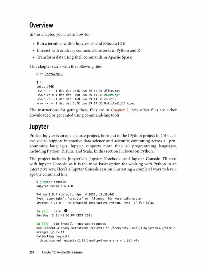
OverviewIn this chapter, you’ll learn how to:

• Run a terminal within JupyterLab and RStudio IDE• Interact with arbitrary command-line tools in Python and R• Transform data using shell commands in Apache Spark

This chapter starts with the following files:

$ cd /data/ch10 $ ltotal 176K-rw-r--r-- 1 dst dst 164K Jun 29 14:36 alice.txt-rwxr-xr-x 1 dst dst 408 Jun 29 14:36 count.py*-rw-r--r-- 1 dst dst 460 Jun 29 14:36 count.R-rw-r--r-- 1 dst dst 1.7K Jun 29 14:36 Untitled1337.ipynb

The instructions for geting these files are in Chapter 2. Any other files are eitherdownloaded or generated using command-line tools.

JupyterProject Jupyter is an open source project, born out of the IPython project in 2014 as itevolved to support interactive data science and scientific computing across all pro‐gramming languages. Jupyter supports more than 40 programming languages,including Python, R, Julia, and Scala. In this section I’ll focus on Python.

The project includes JupyterLab, Jupyter Notebook, and Jupyter Console. I’ll startwith Jupyter Console, as it is the most basic option for working with Python in aninteractive way. Here’s a Jupyter Console session illustrating a couple of ways to lever‐age the command line:

$ jupyter consoleJupyter console 6.4.0 Python 3.9.4 (default, Apr 4 2021, 19:38:44)Type 'copyright', 'credits' or 'license' for more informationIPython 7.23.0 -- An enhanced Interactive Python. Type '?' for help. In [1]: ! date Sun May 2 01:45:06 PM CEST 2021 In [2]: ! pip install --upgrade requestsRequirement already satisfied: requests in /home/dst/.local/lib/python3.9/site-packages (2.25.1)Collecting requests Using cached requests-2.25.1-py2.py3-none-any.whl (61 kB)

200 | Chapter 10: Polyglot Data Science

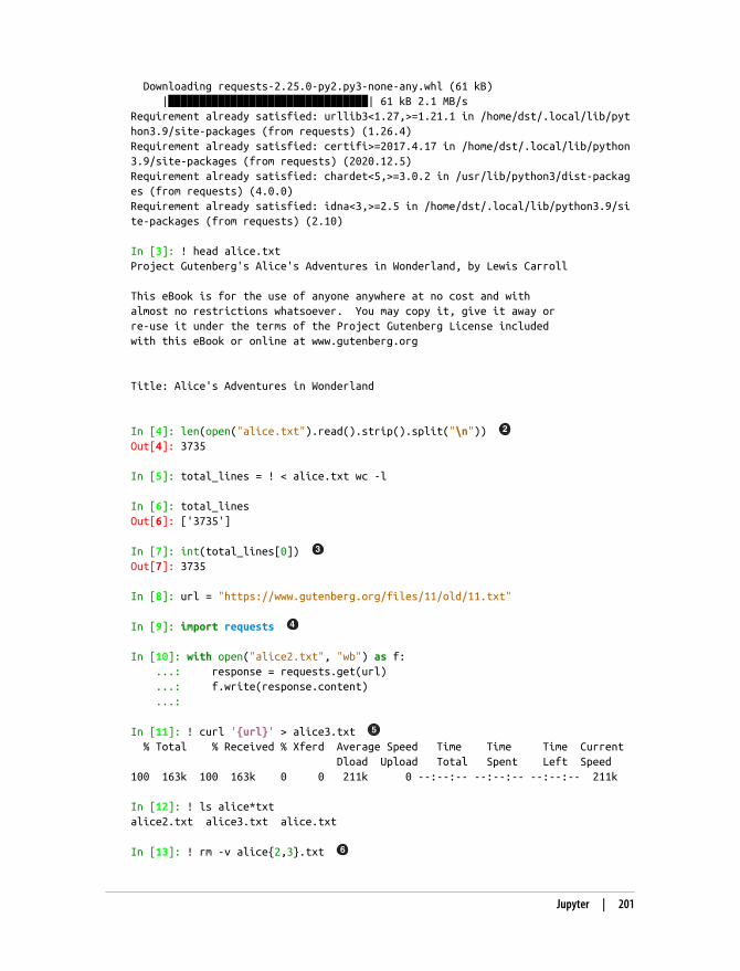
Downloading requests-2.25.0-py2.py3-none-any.whl (61 kB) |████████████████████████████████| 61 kB 2.1 MB/sRequirement already satisfied: urllib3<1.27,>=1.21.1 in /home/dst/.local/lib/python3.9/site-packages (from requests) (1.26.4)Requirement already satisfied: certifi>=2017.4.17 in /home/dst/.local/lib/python3.9/site-packages (from requests) (2020.12.5)Requirement already satisfied: chardet<5,>=3.0.2 in /usr/lib/python3/dist-packages (from requests) (4.0.0)Requirement already satisfied: idna<3,>=2.5 in /home/dst/.local/lib/python3.9/site-packages (from requests) (2.10) In [3]: ! head alice.txtProject Gutenberg's Alice's Adventures in Wonderland, by Lewis Carroll This eBook is for the use of anyone anywhere at no cost and withalmost no restrictions whatsoever. You may copy it, give it away orre-use it under the terms of the Project Gutenberg License includedwith this eBook or online at www.gutenberg.org Title: Alice's Adventures in Wonderland In [4]: len(open("alice.txt").read().strip().split("\n")) Out[4]: 3735 In [5]: total_lines = ! < alice.txt wc -l In [6]: total_linesOut[6]: ['3735'] In [7]: int(total_lines[0]) Out[7]: 3735 In [8]: url = "https://www.gutenberg.org/files/11/old/11.txt" In [9]: import requests In [10]: with open("alice2.txt", "wb") as f: ...: response = requests.get(url) ...: f.write(response.content) ...: In [11]: ! curl '{url}' > alice3.txt % Total % Received % Xferd Average Speed Time Time Time Current Dload Upload Total Spent Left Speed100 163k 100 163k 0 0 211k 0 --:--:-- --:--:-- --:--:-- 211k In [12]: ! ls alice*txtalice2.txt alice3.txt alice.txt In [13]: ! rm -v alice{2,3}.txt

Jupyter | 201

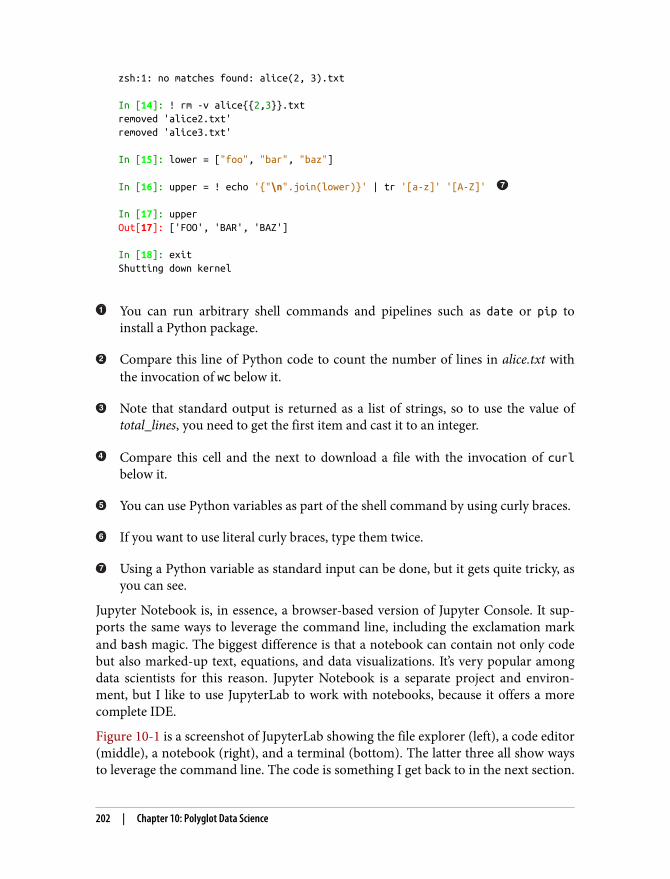
zsh:1: no matches found: alice(2, 3).txt In [14]: ! rm -v alice{{2,3}}.txtremoved 'alice2.txt'removed 'alice3.txt' In [15]: lower = ["foo", "bar", "baz"] In [16]: upper = ! echo '{"\n".join(lower)}' | tr '[a-z]' '[A-Z]' In [17]: upperOut[17]: ['FOO', 'BAR', 'BAZ'] In [18]: exitShutting down kernel

You can run arbitrary shell commands and pipelines such as date or pip toinstall a Python package.

Compare this line of Python code to count the number of lines in alice.txt withthe invocation of wc below it.

Note that standard output is returned as a list of strings, so to use the value oftotal_lines, you need to get the first item and cast it to an integer.

Compare this cell and the next to download a file with the invocation of curlbelow it.

You can use Python variables as part of the shell command by using curly braces.

If you want to use literal curly braces, type them twice.

Using a Python variable as standard input can be done, but it gets quite tricky, asyou can see.

Jupyter Notebook is, in essence, a browser-based version of Jupyter Console. It sup‐ports the same ways to leverage the command line, including the exclamation markand bash magic. The biggest difference is that a notebook can contain not only codebut also marked-up text, equations, and data visualizations. It’s very popular amongdata scientists for this reason. Jupyter Notebook is a separate project and environ‐ment, but I like to use JupyterLab to work with notebooks, because it offers a morecomplete IDE.

Figure 10-1 is a screenshot of JupyterLab showing the file explorer (left), a code editor(middle), a notebook (right), and a terminal (bottom). The latter three all show waysto leverage the command line. The code is something I get back to in the next section.

202 | Chapter 10: Polyglot Data Science

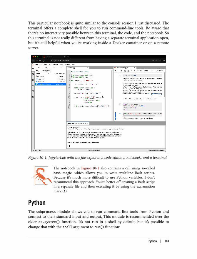
This particular notebook is quite similar to the console session I just discussed. Theterminal offers a complete shell for you to run command-line tools. Be aware thatthere’s no interactivity possible between this terminal, the code, and the notebook. Sothis terminal is not really different from having a separate terminal application open,but it’s still helpful when you’re working inside a Docker container or on a remoteserver.

Figure 10-1. JupyterLab with the file explorer, a code editor, a notebook, and a terminal

The notebook in Figure 10-1 also contains a cell using so-calledbash magic, which allows you to write multiline Bash scripts.Because it’s much more difficult to use Python variables, I don’trecommend this approach. You’re better off creating a Bash scriptin a separate file and then executing it by using the exclamationmark (!).

PythonThe subprocess module allows you to run command-line tools from Python andconnect to their standard input and output. This module is recommended over theolder os.system() function. It’s not run in a shell by default, but it’s possible tochange that with the shell argument to run() function:

Python | 203

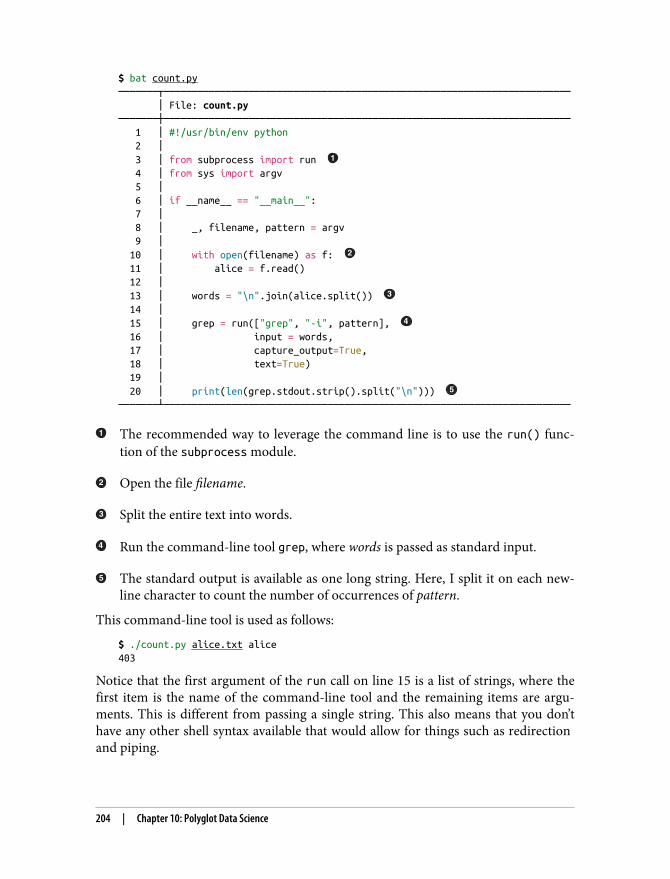
$ bat count.py───────┬──────────────────────────────────────────────────────────────────────── │ File: count.py───────┼──────────────────────────────────────────────────────────────────────── 1 │ #!/usr/bin/env python 2 │ 3 │ from subprocess import run 4 │ from sys import argv 5 │ 6 │ if __name__ == "__main__": 7 │ 8 │ _, filename, pattern = argv 9 │ 10 │ with open(filename) as f: 11 │ alice = f.read() 12 │ 13 │ words = "\n".join(alice.split()) 14 │ 15 │ grep = run(["grep", "-i", pattern], 16 │ input = words, 17 │ capture_output=True, 18 │ text=True) 19 │ 20 │ print(len(grep.stdout.strip().split("\n"))) ───────┴────────────────────────────────────────────────────────────────────────

The recommended way to leverage the command line is to use the run() func‐tion of the subprocess module.

Open the file filename.

Split the entire text into words.

Run the command-line tool grep, where words is passed as standard input.

The standard output is available as one long string. Here, I split it on each new‐line character to count the number of occurrences of pattern.

This command-line tool is used as follows:

$ ./count.py alice.txt alice403

Notice that the first argument of the run call on line 15 is a list of strings, where thefirst item is the name of the command-line tool and the remaining items are argu‐ments. This is different from passing a single string. This also means that you don’thave any other shell syntax available that would allow for things such as redirection and piping.

204 | Chapter 10: Polyglot Data Science

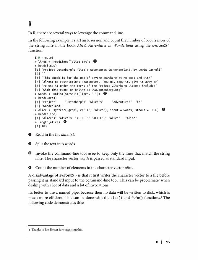
1 Thanks to Jim Hester for suggesting this.

RIn R, there are several ways to leverage the command line.

In the following example, I start an R session and count the number of occurrences ofthe string alice in the book Alice’s Adventures in Wonderland using the system2()function:

$ R --quiet> lines <- readLines("alice.txt") > head(lines)[1] "Project Gutenberg's Alice's Adventures in Wonderland, by Lewis Carroll"[2] ""[3] "This eBook is for the use of anyone anywhere at no cost and with"[4] "almost no restrictions whatsoever. You may copy it, give it away or"[5] "re-use it under the terms of the Project Gutenberg License included"[6] "with this eBook or online at www.gutenberg.org"> words <- unlist(strsplit(lines, " ")) > head(words)[1] "Project" "Gutenberg's" "Alice's" "Adventures" "in"[6] "Wonderland,"> alice <- system2("grep", c("-i", "alice"), input = words, stdout = TRUE) > head(alice)[1] "Alice's" "Alice's" "ALICE'S" "ALICE'S" "Alice" "Alice"> length(alice) [1] 403

Read in the file alice.txt.

Split the text into words.

Invoke the command-line tool grep to keep only the lines that match the stringalice. The character vector words is passed as standard input.

Count the number of elements in the character vector alice.

A disadvantage of system2() is that it first writes the character vector to a file beforepassing it as standard input to the command-line tool. This can be problematic whendealing with a lot of data and a lot of invocations.

It’s better to use a named pipe, because then no data will be written to disk, which ismuch more efficient. This can be done with the pipe() and fifo() functions.1 Thefollowing code demonstrates this:

R | 205

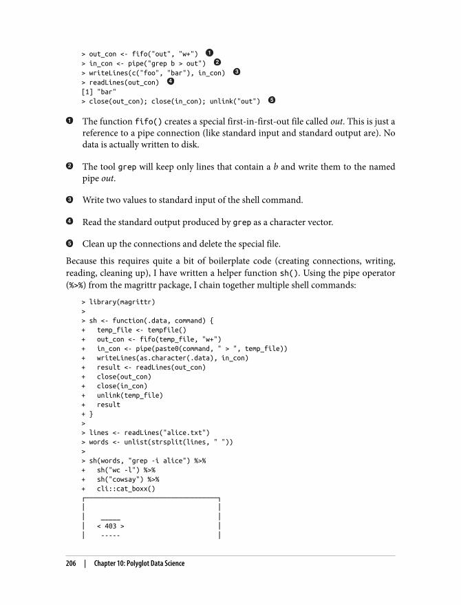
> out_con <- fifo("out", "w+") > in_con <- pipe("grep b > out") > writeLines(c("foo", "bar"), in_con) > readLines(out_con) [1] "bar"> close(out_con); close(in_con); unlink("out")

The function fifo() creates a special first-in-first-out file called out. This is just areference to a pipe connection (like standard input and standard output are). Nodata is actually written to disk.

The tool grep will keep only lines that contain a b and write them to the namedpipe out.

Write two values to standard input of the shell command.

Read the standard output produced by grep as a character vector.

Clean up the connections and delete the special file.

Because this requires quite a bit of boilerplate code (creating connections, writing,reading, cleaning up), I have written a helper function sh(). Using the pipe operator(%>%) from the magrittr package, I chain together multiple shell commands:

> library(magrittr)>> sh <- function(.data, command) {+ temp_file <- tempfile()+ out_con <- fifo(temp_file, "w+")+ in_con <- pipe(paste0(command, " > ", temp_file))+ writeLines(as.character(.data), in_con)+ result <- readLines(out_con)+ close(out_con)+ close(in_con)+ unlink(temp_file)+ result+ }>> lines <- readLines("alice.txt")> words <- unlist(strsplit(lines, " "))>> sh(words, "grep -i alice") %>%+ sh("wc -l") %>%+ sh("cowsay") %>%+ cli::cat_boxx()┌──────────────────────────────────┐│ ││ _____ ││ < 403 > ││ ----- │

206 | Chapter 10: Polyglot Data Science

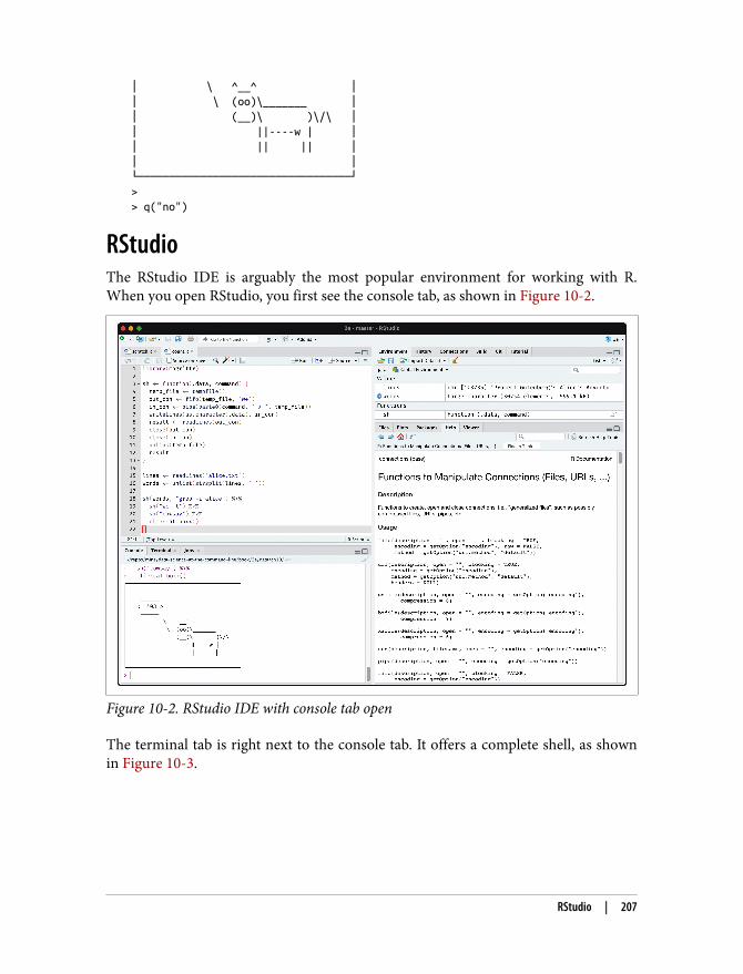
│ \ ^__^ ││ \ (oo)\_______ ││ (__)\ )\/\ ││ ||----w | ││ || || ││ │└──────────────────────────────────┘>> q("no")

RStudioThe RStudio IDE is arguably the most popular environment for working with R.When you open RStudio, you first see the console tab, as shown in Figure 10-2.

Figure 10-2. RStudio IDE with console tab open

The terminal tab is right next to the console tab. It offers a complete shell, as shownin Figure 10-3.

RStudio | 207

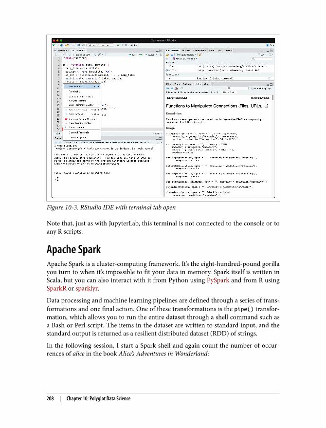
Figure 10-3. RStudio IDE with terminal tab open

Note that, just as with JupyterLab, this terminal is not connected to the console or toany R scripts.

Apache SparkApache Spark is a cluster-computing framework. It’s the eight-hundred-pound gorillayou turn to when it’s impossible to fit your data in memory. Spark itself is written inScala, but you can also interact with it from Python using PySpark and from R usingSparkR or sparklyr.

Data processing and machine learning pipelines are defined through a series of trans‐formations and one final action. One of these transformations is the pipe() transfor‐mation, which allows you to run the entire dataset through a shell command such asa Bash or Perl script. The items in the dataset are written to standard input, and thestandard output is returned as a resilient distributed dataset (RDD) of strings.

In the following session, I start a Spark shell and again count the number of occur‐rences of alice in the book Alice’s Adventures in Wonderland:

208 | Chapter 10: Polyglot Data Science

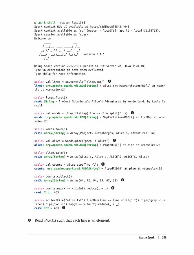
$ spark-shell --master local[6]Spark context Web UI available at http://3d1bec8f2543:4040Spark context available as 'sc' (master = local[6], app id = local-16193763).Spark session available as 'spark'.Welcome to ____ __ / __/__ ___ _____/ /__ _\ \/ _ \/ _ `/ __/ '_/ /___/ .__/\_,_/_/ /_/\_\ version 3.1.1 /_/ Using Scala version 2.12.10 (OpenJDK 64-Bit Server VM, Java 11.0.10)Type in expressions to have them evaluated.Type :help for more information. scala> val lines = sc.textFile("alice.txt") lines: org.apache.spark.rdd.RDD[String] = alice.txt MapPartitionsRDD[1] at textFile at <console>:24 scala> lines.first()res0: String = Project Gutenberg's Alice's Adventures in Wonderland, by Lewis Carroll scala> val words = lines.flatMap(line => line.split(" ")) words: org.apache.spark.rdd.RDD[String] = MapPartitionsRDD[2] at flatMap at <console>:25 scala> words.take(5)res1: Array[String] = Array(Project, Gutenberg's, Alice's, Adventures, in) scala> val alice = words.pipe("grep -i alice") alice: org.apache.spark.rdd.RDD[String] = PipedRDD[3] at pipe at <console>:25 scala> alice.take(5)res2: Array[String] = Array(Alice's, Alice's, ALICE'S, ALICE'S, Alice) scala> val counts = alice.pipe("wc -l") counts: org.apache.spark.rdd.RDD[String] = PipedRDD[4] at pipe at <console>:25 scala> counts.collect()res3: Array[String] = Array(64, 72, 94, 93, 67, 13) scala> counts.map(x => x.toInt).reduce(_ + _) res4: Int = 403 scala> sc.textFile("alice.txt").flatMap(line => line.split(" ")).pipe("grep -i alice").pipe("wc -l").map(x => x.toInt).reduce(_ + _)res5: Int = 403

Read alice.txt such that each line is an element.

Apache Spark | 209

Split each element on spaces. In other words, each line is split into words.

Pipe each partition through grep to keep only the elements that match the stringalice.

Pipe each partition through wc to count the number of elements.

There’s one count for each partition.

Sum all counts to get a final count. Note that elements first need to be convertedfrom strings to integers.

This shows the preceding steps combined into a single command.

The pipe() transformation is also available in PySpark, SparkR,and sparklyr.

If you want to use a custom command-line tool in your pipeline, then you need tomake sure that it’s present on all nodes in the cluster (known as the executors). Oneway to do this is to specify the filename(s) with the --files option when you’re sub‐mitting Spark applications using spark-submit.

Bill Chambers and Matei Zaharia (the original authors of Apache Spark) mention intheir book Spark: The Definitive Guide (O’Reilly) that “[t]he pipe method is probablyone of Spark’s more interesting methods.” That’s quite the compliment! I think it’sfantastic that the developers of Apache Spark added the ability to leverage a 50-year-old technology.

SummaryIn this chapter you learned several ways to leverage the command line in other situa‐tions, including programming languages and other environments. It’s important torealize that the command line doesn’t exist in a vacuum. What matters most is thatyou use tools, sometimes in combination with one another, that reliably get the jobdone.

Now that we’ve had the four OSEMN chapters and the four intermezzo chapters, it’stime to wrap this up in the final chapter.

210 | Chapter 10: Polyglot Data Science

For Further ExplorationThere are also ways to integrate two programming languages directly without the useof the command line. For example, the reticulate package in R allows you to interfacewith Python directly.

For Further Exploration | 211

CHAPTER 11

Conclusion

In this final chapter, the book comes to a close. I’ll first recap what I’ve discussed inthe previous 10 chapters, and then I’ll offer you three pieces of advice and providesome resources to further explore the related topics we touched on. Finally, in caseyou have any questions, comments, or new command-line tools to share, I provide afew ways to get in touch with me.

Let’s RecapThis book explored the power of using the command line to do data science. I find itan interesting observation that the challenges posed by this relatively young field canbe tackled using such a time-tested technology. I hope that you now see what thecommand line is capable of. The many command-line tools offer all sorts of possibili‐ties that are well suited to the variety of tasks encompassing data science.

There are many definitions of data science available. In Chapter 1, I introduced thefive-step OSEMN model as defined by Hilary Mason and Chris Wiggins, because it isa very practical one that translates to very specific tasks. The acronym OSEMN standsfor obtaining, scrubbing, exploring, modeling, and interpreting data. Chapter 1 alsoexplained why the command line is very suitable for doing these data science tasks.

In Chapter 2, I explained how you can get all the tools used in this book. Chapter 2also provided an introduction to the essential tools and concepts of the commandline.

The four OSEMN model chapters focused on performing those practical tasks usingthe command line. I did not devote a chapter to the fifth step, interpreting data,because quite frankly, the computer—let alone the command line—is of very little usehere. I have, however, provided some pointers for further reading on this topic.

213

In the four intermezzo chapters, we looked at some broader topics of doing data sci‐ence at the command line, topics that are not really specific to a particular step. InChapter 4, I explained how you can turn one-liners and existing code into reusablecommand-line tools. In Chapter 6, I described how you can manage your data work‐flow using a tool called make. In Chapter 8, I demonstrated how ordinary command-line tools and pipelines can be run in parallel using GNU Parallel. In Chapter 10, Ishowed that the command line doesn’t exist in a vacuum but can be leveraged fromother programming languages and environments. The topics discussed in these inter‐mezzo chapters can be applied at any point in your data workflow.

It’s impossible to demonstrate all the command-line tools that are available and rele‐vant for doing data science. New tools are created on a daily basis. As you may havecome to understand by now, this book is more about the idea of using the commandline rather than giving you an exhaustive list of tools.

Three Pieces of AdviceYou probably spent a good bit of time reading these chapters and perhaps also follow‐ing along with the code examples. In the hope that it maximizes the return on thisinvestment and increases the probability that you’ll continue to incorporate the com‐mand line into your data science workflow, I would like to offer you three pieces ofadvice: (1) be patient, (2) be creative, and (3) be practical. In the next three subsec‐tions I elaborate on each piece of advice.

Be PatientThe first piece of advice that I can give is to be patient. Working with data on thecommand line is different from using a programming language, and therefore itrequires a different mindset.

Moreover, the command-line tools themselves are not without their quirks andinconsistencies. This is partly because they have been developed by many differentpeople over the course of multiple decades. If you ever find yourself at a loss regard‐ing their mind-dazzling options, don’t forget to use --help, man, tldr, or your favor‐ite search engine to learn more.

Still, especially in the beginning, working on the command line can be a frustratingexperience. Trust me, you’ll become more proficient as you practice using the com‐mand line and its tools. The command line has been around for many decades andwill be around for many more to come. It’s a worthwhile investment.

214 | Chapter 11: Conclusion

Be CreativeThe second, related piece of advice is to be creative. The command line is very flexi‐ble. By combining the command-line tools, you can accomplish more than you mightthink.

I encourage you to not immediately fall back onto your programming language. Andwhen you do have to use a programming language, think about whether the code canbe generalized or reused in some way; if so, consider creating your own command-line tool with that code using the steps I discussed in Chapter 4. If you believe yourtool may be beneficial for others, you could even go one step further by making itopen source. Maybe there’s a step you know how to perform at the command line, butyou would rather not leave the comfort of the main programming language or envi‐ronment you’re working in. Perhaps you can use one of the approaches listed inChapter 10.

Be PracticalThe third piece of advice is to be practical. Being practical is related to being creativebut deserves a separate explanation. In the previous subsection, I mentioned that youshould not immediately fall back to a programming language. Of course, the com‐mand line has its limits. Throughout the book, I have emphasized that the commandline should be regarded as a companion approach to doing data science.

I’ve discussed four steps for doing data science at the command line. In practice, theapplicability of the command line is higher for step 1 than it is for step 4. You shoulduse whichever approach works best for the task at hand. And it’s perfectly fine to mixand match approaches at any point in your workflow. As I’ve shown in Chapter 10,the command line is wonderful at being integrated with other approaches, program‐ming languages, and statistical environments. There’s a certain trade-off with eachapproach, and part of becoming proficient at the command line is to learn when touse which approach.

In conclusion, when you’re patient, creative, and practical, the command line willmake you a more efficient and productive data scientist.

Where to Go from HereAs this book is on the intersection of the command line and data science, manyrelated topics have only been touched on. Now it’s up to you to further explore thesetopics. The following subsections provide a list of topics and suggested resources toconsult.

Where to Go from Here | 215

The Command Line• The Linux Command Line: A Complete Introduction, 2nd ed., by William Shotts

(San Franciscio: No Starch, 2019)• Unix Power Tools, 3rd ed., by Shelley Powers, Jerry Peek, Tim O’Reilly, and Mike

Loukides (Sebastopol, CA: O’Reilly, 2002)• Learning the vi and Vim Editors, 7th ed., by Arnold Robbins, Elbert Hannah, and

Linda Lamb (Sebastopol, CA: O’Reilly, 2008)

Shell Programming• Classic Shell Scripting by Arnold Robbins and Nelson H. F. Beebe (Sebastopol,

CA: O’Reilly, 2005)• Wicked Cool Shell Scripts, 2nd ed., by Dave Taylor and Brandon Perry (San Fran‐

ciscio: No Starch, 2017)• bash Cookbook, 2nd ed., by Carl Albing and JP Vossen (Sebastopol, CA: O’Reilly,

2017)

Python, R, and SQL• Learn Python 3 the Hard Way by Zed A. Shaw (Boston: Addison-Wesley, 2017)• Python for Data Analysis, 2nd ed., by Wes McKinney (Sebastopol, CA: O’Reilly,

2017)• Data Science from Scratch, 2nd ed., by Joel Grus (Sebastopol, CA: O’Reilly, 2019)• R for Data Science by Hadley Wickham and Garrett Grolemund (Sebastopol, CA:

O’Reilly, 2016)• R for Everyone, 2nd ed., by Jared P. Lander (Boston: Addison-Wesley, 2017)• Sams Teach Yourself SQL in 10 Minutes a Day, 5th ed., by Ben Forta (Hoboken:

Sams, 2020)

APIs• Mining the Social Web, 3rd ed., by Matthew A. Russell and Mikhail Klassen

(Sebastopol, CA: O’Reilly, 2019)• Data Source Handbook by Pete Warden (Sebastopol, CA: O’Reilly, 2011)

216 | Chapter 11: Conclusion

Machine Learning• Python Machine Learning, 3rd ed., by Sebastian Raschka and Vahid Mirjalili (Bir‐

mingham, UK: Packt, 2019)• Pattern Recognition and Machine Learning by Christopher M. Bishop (New York:

Springer, 2006)• Information Theory, Inference, and Learning Algorithms by David J. C. MacKay

(Cambridge, UK: Cambridge University Press, 2003)

Getting in TouchThis book would not have been possible without the many people who created thecommand line and the numerous tools. It’s safe to say that the current ecosystem ofcommand-line tools for data science is a community effort. I have only been able togive you a glimpse of the many command-line tools available. New ones are createdevery day, and perhaps some day you will create one yourself, in which case, I wouldlove to hear from you. I’d also appreciate it if you would drop me a line whenever youhave a question, comment, or suggestion. There are a few ways to get in touch:

• Email: jeroen@jeroenjanssens.com• Twitter: @jeroenhjanssens• Book website: https://datascienceatthecommandline.com• Book GitHub repository: https://github.com/jeroenjanssens/data-science-at-the-

command-line

Thank you.

Getting in Touch | 217

APPENDIX

List of Command-Line Tools

This is an overview of all the command-line tools discussed in this book. Thisincludes binary executables, interpreted scripts, and Z Shell builtins and keywords.For each command-line tool, the following information, when available and appro‐priate, is provided:

• The actual command to type at the command line• A description• The version used in the book• The year that version was released• The primary author(s)• A website to find more information• How to obtain help• An example usage

All command-line tools listed here are included in the Docker image. See Chapter 2for instructions on how to set it up. Please note that citing open source software is nottrivial, and that some information may be missing or incorrect.

aliasDefine or display aliases. alias is a Z shell builtin.

$ type aliasalias is a shell builtin $ man zshbuiltins | grep -A 10 alias

219

$ alias ll='ls --color -lhF --group-directories-first' $ alias python=python3

awkPattern scanning and text processing language. awk (version 1.3.4) by Mike D.Brennan and Thomas E. Dickey (2019). More information: https://invisible-island.net/mawk.

$ type awkawk is /usr/bin/awk $ man awk $ seq 5 | awk '{sum+=$1} END {print sum}'15

awsUnified tool to manage AWS services. aws (version 2.1.32) by Amazon Web Services(2021). More information: https://aws.amazon.com/cli.

$ type awsaws is /usr/local/bin/aws $ aws --help

bashGNU Bourne-Again Shell. bash (version 5.0.17) by Brian Fox and Chet Ramey(2019). More information: https://www.gnu.org/software/bash.

$ type bashbash is /usr/bin/bash $ man bash

batA cat clone with syntax highlighting and Git integration. bat (version 0.18.0) byDavid Peter (2021). More information: https://github.com/sharkdp/bat.

$ type batbat is an alias for bat --tabs 8 --paging never $ man bat

220 | List of Command-Line Tools

bcAn arbitrary precision calculator language. bc (version 1.07.1) by Philip A. Nelson(2017). More information: https://www.gnu.org/software/bc.

$ type bcbc is /usr/bin/bc $ man bc $ bc -l <<< 'e(1)'2.71828182845904523536

bodyApply expression to all but the first line. body (version 0.1) by Jeroen Janssens (2021).More information: https://github.com/jeroenjanssens/dsutils.

$ type bodybody is /usr/bin/dsutils/body $ seq 10 | header -a 'values' | body shufvalues75261039814

catConcatenate files and print on the standard output. cat (version 8.30) by TorbjornGranlund and Richard M. Stallman (2018). More information: https://www.gnu.org/software/coreutils.

$ type catcat is /usr/bin/cat $ man cat $ cat *.log > all.log

List of Command-Line Tools | 221

cdChange the shell working directory. cd is a Z shell builtin.

$ type cdcd is a shell builtin $ man zshbuiltins | grep -A 10 cd $ cd ~ $ pwd/home/dst $ cd .. $ pwd/home $ cd /data/ch01

chmodChange file mode bits. chmod (version 8.30) by David MacKenzie and Jim Meyering(2018). I use chmod in Chapter 4 to make a tool executable. More information: https://www.gnu.org/software/coreutils.

$ type chmodchmod is /usr/bin/chmod $ man chmod $ chmod u+x script.sh

colsApply command to a subset of columns. cols (version 0.1) by Jeroen Janssens (2021).More information: https://github.com/jeroenjanssens/dsutils.

$ type colscols is /usr/bin/dsutils/cols

columnColumnate lists. column (version 2.36.1) by Karel Zak (2021). More information:https://www.kernel.org/pub/linux/utils/util-linux.

$ type columncolumn is /usr/bin/column

222 | List of Command-Line Tools

cowsayConfigurable speaking cow. cowsay (version 3.0.3) by Tony Monroe (1999). Moreinformation: https://github.com/tnalpgge/rank-amateur-cowsay.

$ type cowsaycowsay is /usr/bin/cowsay $ man cowsay $ echo 'The command line is awesome!' | cowsay ______________________________< The command line is awesome! > ------------------------------ \ ^__^ \ (oo)\_______ (__)\ )\/\ ||----w | || ||

cpCopy files and directories. cp (version 8.30) by Torbjorn Granlund, David MacKen‐zie, and Jim Meyering (2018). More information: https://www.gnu.org/software/coreutils.

$ type cpcp is /usr/bin/cp $ man cp $ cp -r ~/Downloads/*.xlsx /data

csv2vwConvert CSV to Vowpal Wabbit format. csv2vw (version 0.1) by Jeroen Janssens(2021). More information: https://github.com/jeroenjanssens/dsutils.

$ type csv2vwcsv2vw is /usr/bin/dsutils/csv2vw

csvcutFilter and truncate CSV files. csvcut (version 1.0.5) by Christopher Groskopf (2020).More information: https://csvkit.rtfd.org.

List of Command-Line Tools | 223

$ type csvcutcsvcut is /usr/bin/csvcut $ csvcut --help $ csvcut -c bill,tip /data/ch05/tips.csv | trimbill,tip16.99,1.0110.34,1.6621.01,3.523.68,3.3124.59,3.6125.29,4.718.77,2.026.88,3.1215.04,1.96… with 235 more lines

csvgrepSearch CSV files. csvgrep (version 1.0.5) by Christopher Groskopf (2020). Moreinformation: https://csvkit.rtfd.org.

$ type csvgrepcsvgrep is /usr/bin/csvgrep $ csvgrep --help

csvjoinExecute a SQL-like join to merge CSV files on a specified column or columns.csvjoin (version 1.0.5) by Christopher Groskopf (2020). More information: https://csvkit.rtfd.org.

$ type csvjoincsvjoin is /usr/bin/csvjoin $ csvjoin --help

csvlookRender a CSV file in the console as a Markdown-compatible, fixed-width table.csvlook (version 1.0.5) by Christopher Groskopf (2020). More information: https://csvkit.rtfd.org.

$ type csvlookcsvlook is a shell function $ csvlook --help

224 | List of Command-Line Tools

$ csvlook /data/ch05/tips.csv│ bill │ tip │ sex │ smoker │ day │ time │ size │├───────┼───────┼────────┼────────┼──────┼────────┼──────┤│ 16.99 │ 1.01 │ Female │ False │ Sun │ Dinner │ 2 ││ 10.34 │ 1.66 │ Male │ False │ Sun │ Dinner │ 3 ││ 21.01 │ 3.50 │ Male │ False │ Sun │ Dinner │ 3 ││ 23.68 │ 3.31 │ Male │ False │ Sun │ Dinner │ 2 ││ 24.59 │ 3.61 │ Female │ False │ Sun │ Dinner │ 4 ││ 25.29 │ 4.71 │ Male │ False │ Sun │ Dinner │ 4 ││ 8.77 │ 2.00 │ Male │ False │ Sun │ Dinner │ 2 ││ 26.88 │ 3.12 │ Male │ False │ Sun │ Dinner │ 4 │… with 236 more lines

csvquoteEnable common Unix utlities to work correctly with CSV data. csvquote (version0.1) by Dan Brown (2018). More information: https://github.com/dbro/csvquote.

$ type csvquotecsvquote is /usr/local/bin/csvquote

csvsortSort CSV files. csvsort (version 1.0.5) by Christopher Groskopf (2020). More infor‐mation: https://csvkit.rtfd.org.

$ type csvsortcsvsort is /usr/bin/csvsort $ csvsort --help

csvsqlExecute SQL statements on CSV files. csvsql (version 1.0.5) by Christopher Gros‐kopf (2020). More information: https://csvkit.rtfd.org.

$ type csvsqlcsvsql is /usr/bin/csvsql $ csvsql --help

csvstackStack up the rows from multiple CSV files. csvstack (version 1.0.5) by ChristopherGroskopf (2020). More information: https://csvkit.rtfd.org.

$ type csvstackcsvstack is /usr/bin/csvstack

List of Command-Line Tools | 225

$ csvstack --help

csvstatPrint descriptive statistics for each column in a CSV file. csvstat (version 1.0.5) byChristopher Groskopf (2020). More information: https://csvkit.rtfd.org.

$ type csvstatcsvstat is /usr/bin/csvstat $ csvstat --help

curlTransfer a URL. curl (version 7.68.0) by Daniel Stenberg (2016). More information:https://curl.haxx.se.

$ type curlcurl is /usr/bin/curl $ man curl

cutRemove sections from each line of files. cut (version 8.30) by David M. Ihnat, DavidMacKenzie, and Jim Meyering (2019). More information: https://www.gnu.org/software/coreutils.

$ type cutcut is /usr/bin/cut $ man cut

displayDisplay an image or image sequence on any X server. display (version 6.9.10-23) byImageMagick Studio LLC (2019). More information: https://imagemagick.org.

$ type displaydisplay is a shell function

226 | List of Command-Line Tools

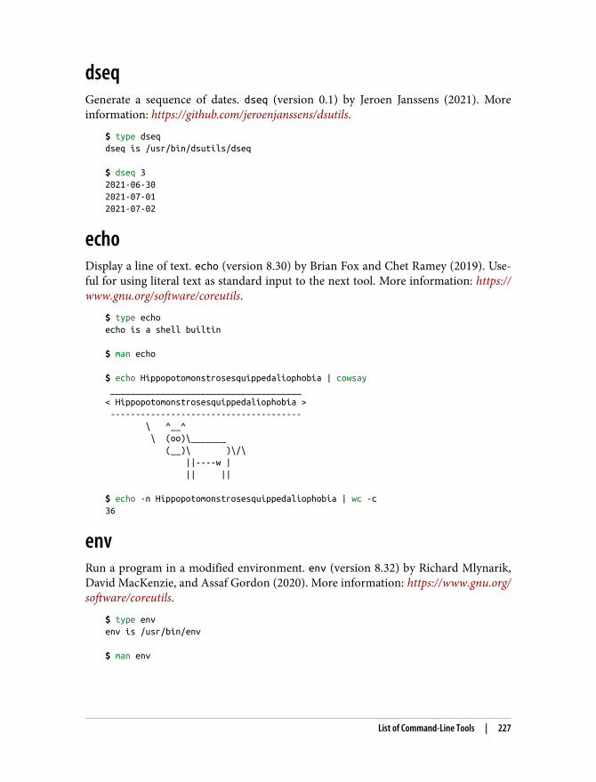
dseqGenerate a sequence of dates. dseq (version 0.1) by Jeroen Janssens (2021). Moreinformation: https://github.com/jeroenjanssens/dsutils.

$ type dseqdseq is /usr/bin/dsutils/dseq $ dseq 32021-06-302021-07-012021-07-02

echoDisplay a line of text. echo (version 8.30) by Brian Fox and Chet Ramey (2019). Use‐ful for using literal text as standard input to the next tool. More information: https://www.gnu.org/software/coreutils.

$ type echoecho is a shell builtin $ man echo $ echo Hippopotomonstrosesquippedaliophobia | cowsay ______________________________________< Hippopotomonstrosesquippedaliophobia > -------------------------------------- \ ^__^ \ (oo)\_______ (__)\ )\/\ ||----w | || || $ echo -n Hippopotomonstrosesquippedaliophobia | wc -c36

envRun a program in a modified environment. env (version 8.32) by Richard Mlynarik,David MacKenzie, and Assaf Gordon (2020). More information: https://www.gnu.org/software/coreutils.

$ type envenv is /usr/bin/env $ man env

List of Command-Line Tools | 227

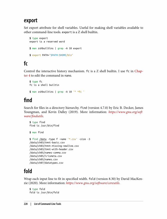
exportSet export attribute for shell variables. Useful for making shell variables available toother command-line tools. export is a Z shell builtin.

$ type exportexport is a reserved word $ man zshbuiltins | grep -A 10 export $ export PATH="$PATH:$HOME/bin"

fcControl the interactive history mechanism. fc is a Z shell builtin. I use fc in Chap‐ter 4 to edit the command in nano.

$ type fcfc is a shell builtin $ man zshbuiltins | grep -A 10 '^ *fc '

findSearch for files in a directory hierarchy. find (version 4.7.0) by Eric B. Decker, JamesYoungman, and Kevin Dalley (2019). More information: https://www.gnu.org/software/findutils.

$ type findfind is /usr/bin/find $ man find $ find /data -type f -name '*.csv' -size -3/data/ch03/tmnt-basic.csv/data/ch03/tmnt-missing-newline.csv/data/ch03/tmnt-with-header.csv/data/ch05/names-comma.csv/data/ch05/irismeta.csv/data/ch05/names.csv/data/ch07/datatypes.csv

foldWrap each input line to fit in specified width. fold (version 8.30) by David MacKen‐zie (2020). More information: https://www.gnu.org/software/coreutils.

$ type foldfold is /usr/bin/fold

228 | List of Command-Line Tools

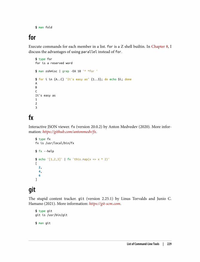
$ man fold

forExecute commands for each member in a list. for is a Z shell builtin. In Chapter 8, Idiscuss the advantages of using parallel instead of for.

$ type forfor is a reserved word $ man zshmisc | grep -EA 10 '^ *for ' $ for i in {A..C} "It's easy as" {1..3}; do echo $i; doneABCIt's easy as123

fxInteractive JSON viewer. fx (version 20.0.2) by Anton Medvedev (2020). More infor‐mation: https://github.com/antonmedv/fx.

$ type fxfx is /usr/local/bin/fx $ fx --help $ echo '[1,2,3]' | fx 'this.map(x => x * 2)'[ 2, 4, 6]

gitThe stupid content tracker. git (version 2.25.1) by Linus Torvalds and Junio C.Hamano (2021). More information: https://git-scm.com.

$ type gitgit is /usr/bin/git $ man git

List of Command-Line Tools | 229

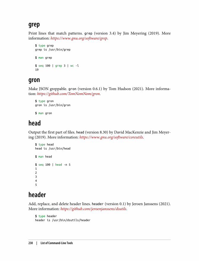
grepPrint lines that match patterns. grep (version 3.4) by Jim Meyering (2019). Moreinformation: https://www.gnu.org/software/grep.

$ type grepgrep is /usr/bin/grep $ man grep $ seq 100 | grep 3 | wc -l19

gronMake JSON greppable. gron (version 0.6.1) by Tom Hudson (2021). More informa‐tion: https://github.com/TomNomNom/gron.

$ type grongron is /usr/bin/gron $ man gron

headOutput the first part of files. head (version 8.30) by David MacKenzie and Jim Meyer‐ing (2019). More information: https://www.gnu.org/software/coreutils.

$ type headhead is /usr/bin/head $ man head $ seq 100 | head -n 512345

headerAdd, replace, and delete header lines. header (version 0.1) by Jeroen Janssens (2021).More information: https://github.com/jeroenjanssens/dsutils.

$ type headerheader is /usr/bin/dsutils/header

230 | List of Command-Line Tools

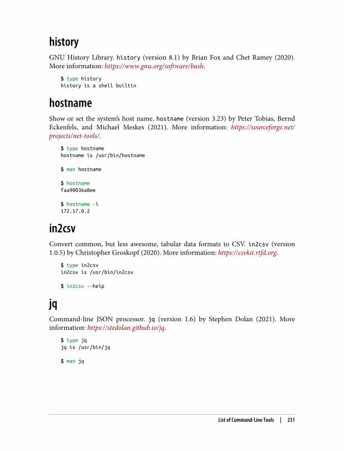
historyGNU History Library. history (version 8.1) by Brian Fox and Chet Ramey (2020).More information: https://www.gnu.org/software/bash.

$ type historyhistory is a shell builtin

hostnameShow or set the system’s host name. hostname (version 3.23) by Peter Tobias, BerndEckenfels, and Michael Meskes (2021). More information: https://sourceforge.net/projects/net-tools/.

$ type hostnamehostname is /usr/bin/hostname $ man hostname $ hostnamefaa90036a8ee $ hostname -i172.17.0.2

in2csvConvert common, but less awesome, tabular data formats to CSV. in2csv (version1.0.5) by Christopher Groskopf (2020). More information: https://csvkit.rtfd.org.

$ type in2csvin2csv is /usr/bin/in2csv $ in2csv --help

jqCommand-line JSON processor. jq (version 1.6) by Stephen Dolan (2021). Moreinformation: https://stedolan.github.io/jq.

$ type jqjq is /usr/bin/jq $ man jq

List of Command-Line Tools | 231

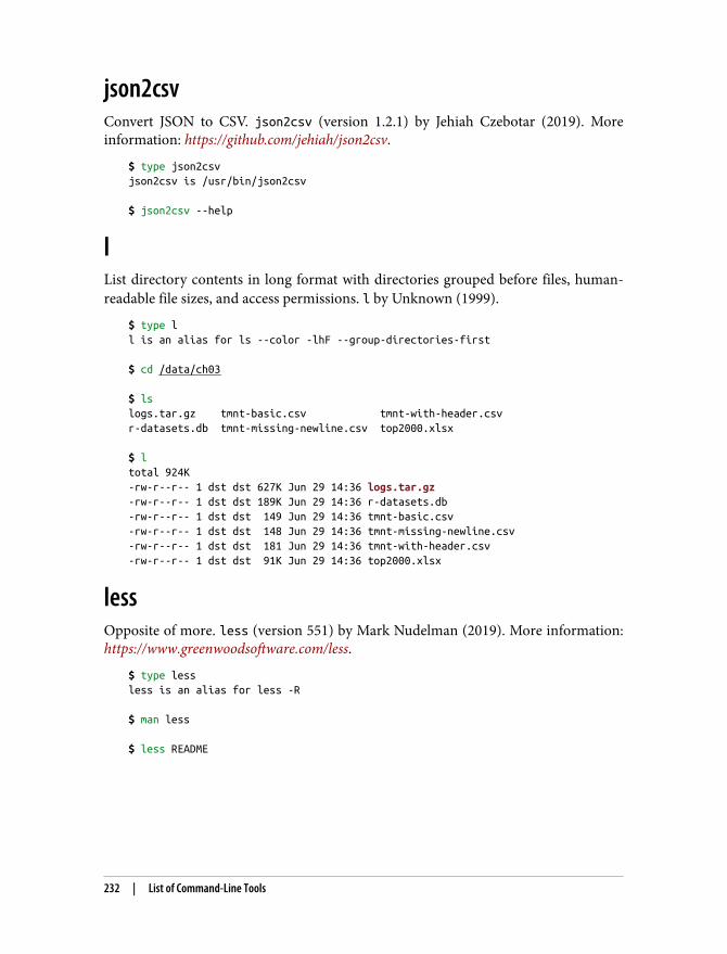
json2csvConvert JSON to CSV. json2csv (version 1.2.1) by Jehiah Czebotar (2019). Moreinformation: https://github.com/jehiah/json2csv.

$ type json2csvjson2csv is /usr/bin/json2csv $ json2csv --help

lList directory contents in long format with directories grouped before files, human-readable file sizes, and access permissions. l by Unknown (1999).

$ type ll is an alias for ls --color -lhF --group-directories-first $ cd /data/ch03 $ lslogs.tar.gz tmnt-basic.csv tmnt-with-header.csvr-datasets.db tmnt-missing-newline.csv top2000.xlsx $ ltotal 924K-rw-r--r-- 1 dst dst 627K Jun 29 14:36 logs.tar.gz-rw-r--r-- 1 dst dst 189K Jun 29 14:36 r-datasets.db-rw-r--r-- 1 dst dst 149 Jun 29 14:36 tmnt-basic.csv-rw-r--r-- 1 dst dst 148 Jun 29 14:36 tmnt-missing-newline.csv-rw-r--r-- 1 dst dst 181 Jun 29 14:36 tmnt-with-header.csv-rw-r--r-- 1 dst dst 91K Jun 29 14:36 top2000.xlsx

lessOpposite of more. less (version 551) by Mark Nudelman (2019). More information:https://www.greenwoodsoftware.com/less.

$ type lessless is an alias for less -R $ man less $ less README

232 | List of Command-Line Tools

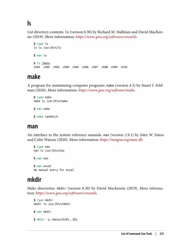
lsList directory contents. ls (version 8.30) by Richard M. Stallman and David MacKen‐zie (2019). More information: https://www.gnu.org/software/coreutils.

$ type lsls is /usr/bin/ls $ man ls $ ls /datach01 ch02 ch03 ch04 ch05 ch06 ch07 ch08 ch09 ch10

makeA program for maintaining computer programs. make (version 4.3) by Stuart I. Feld‐man (2020). More information: https://www.gnu.org/software/make.

$ type makemake is /usr/bin/make $ man make $ make sandwich

manAn interface to the system reference manuals. man (version 2.9.1) by John W. Eatonand Colin Watson (2020). More information: https://nongnu.org/man-db.

$ type manman is /usr/bin/man $ man man $ man excelNo manual entry for excel

mkdirMake directories. mkdir (version 8.30) by David MacKenzie (2019). More informa‐tion: https://www.gnu.org/software/coreutils.

$ type mkdirmkdir is /usr/bin/mkdir $ man mkdir $ mkdir -p /data/ch{01..10}

List of Command-Line Tools | 233

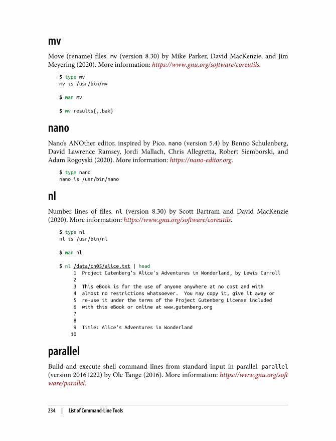
mvMove (rename) files. mv (version 8.30) by Mike Parker, David MacKenzie, and JimMeyering (2020). More information: https://www.gnu.org/software/coreutils.

$ type mvmv is /usr/bin/mv $ man mv $ mv results{,.bak}

nanoNano’s ANOther editor, inspired by Pico. nano (version 5.4) by Benno Schulenberg,David Lawrence Ramsey, Jordi Mallach, Chris Allegretta, Robert Siemborski, andAdam Rogoyski (2020). More information: https://nano-editor.org.

$ type nanonano is /usr/bin/nano

nlNumber lines of files. nl (version 8.30) by Scott Bartram and David MacKenzie(2020). More information: https://www.gnu.org/software/coreutils.

$ type nlnl is /usr/bin/nl $ man nl $ nl /data/ch05/alice.txt | head 1 Project Gutenberg's Alice's Adventures in Wonderland, by Lewis Carroll 2 3 This eBook is for the use of anyone anywhere at no cost and with 4 almost no restrictions whatsoever. You may copy it, give it away or 5 re-use it under the terms of the Project Gutenberg License included 6 with this eBook or online at www.gutenberg.org 7 8 9 Title: Alice's Adventures in Wonderland 10

parallelBuild and execute shell command lines from standard input in parallel. parallel(version 20161222) by Ole Tange (2016). More information: https://www.gnu.org/software/parallel.

234 | List of Command-Line Tools

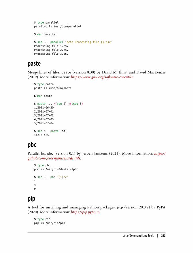
$ type parallelparallel is /usr/bin/parallel $ man parallel $ seq 3 | parallel "echo Processing file {}.csv"Processing file 1.csvProcessing file 2.csvProcessing file 3.csv

pasteMerge lines of files. paste (version 8.30) by David M. Ihnat and David MacKenzie(2019). More information: https://www.gnu.org/software/coreutils.

$ type pastepaste is /usr/bin/paste $ man paste $ paste -d, <(seq 5) <(dseq 5)1,2021-06-302,2021-07-013,2021-07-024,2021-07-035,2021-07-04 $ seq 5 | paste -sd+1+2+3+4+5

pbcParallel bc. pbc (version 0.1) by Jeroen Janssens (2021). More information: https://github.com/jeroenjanssens/dsutils.

$ type pbcpbc is /usr/bin/dsutils/pbc $ seq 3 | pbc '{1}^2'149

pipA tool for installing and managing Python packages. pip (version 20.0.2) by PyPA(2020). More information: https://pip.pypa.io.

$ type pippip is /usr/bin/pip

List of Command-Line Tools | 235

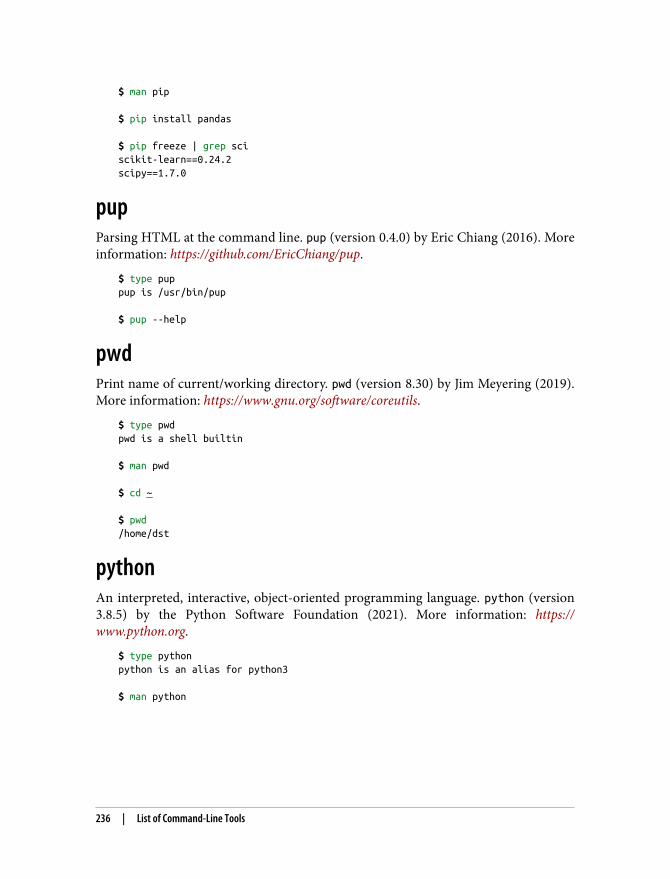
$ man pip $ pip install pandas $ pip freeze | grep sciscikit-learn==0.24.2scipy==1.7.0

pupParsing HTML at the command line. pup (version 0.4.0) by Eric Chiang (2016). Moreinformation: https://github.com/EricChiang/pup.

$ type puppup is /usr/bin/pup $ pup --help

pwdPrint name of current/working directory. pwd (version 8.30) by Jim Meyering (2019).More information: https://www.gnu.org/software/coreutils.

$ type pwdpwd is a shell builtin $ man pwd $ cd ~ $ pwd/home/dst

pythonAn interpreted, interactive, object-oriented programming language. python (version3.8.5) by the Python Software Foundation (2021). More information: https://www.python.org.

$ type pythonpython is an alias for python3 $ man python

236 | List of Command-Line Tools

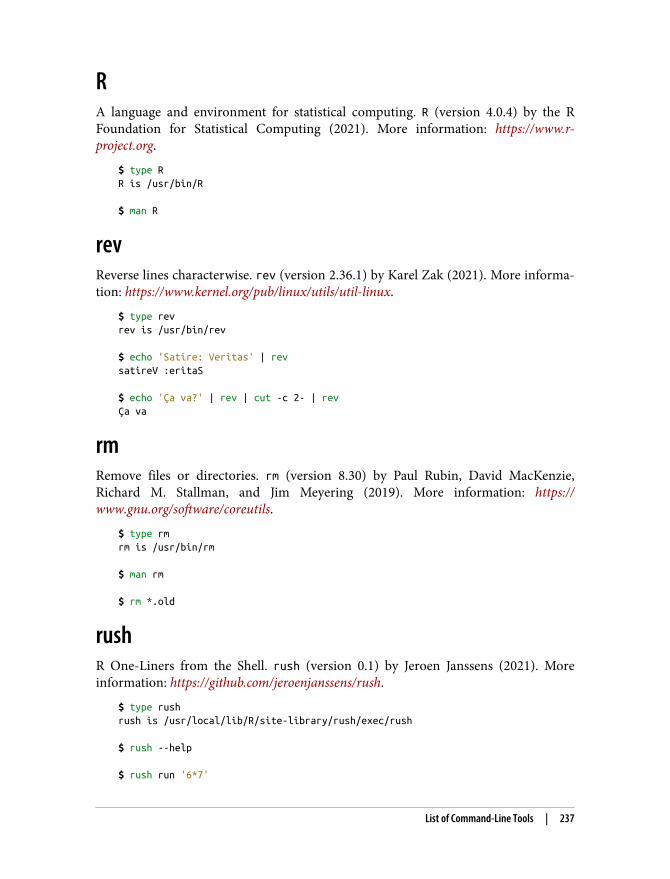
RA language and environment for statistical computing. R (version 4.0.4) by the RFoundation for Statistical Computing (2021). More information: https://www.r-project.org.

$ type RR is /usr/bin/R $ man R

revReverse lines characterwise. rev (version 2.36.1) by Karel Zak (2021). More informa‐tion: https://www.kernel.org/pub/linux/utils/util-linux.

$ type revrev is /usr/bin/rev $ echo 'Satire: Veritas' | revsatireV :eritaS $ echo 'Ça va?' | rev | cut -c 2- | revÇa va

rmRemove files or directories. rm (version 8.30) by Paul Rubin, David MacKenzie,Richard M. Stallman, and Jim Meyering (2019). More information: https://www.gnu.org/software/coreutils.

$ type rmrm is /usr/bin/rm $ man rm $ rm *.old

rushR One-Liners from the Shell. rush (version 0.1) by Jeroen Janssens (2021). Moreinformation: https://github.com/jeroenjanssens/rush.

$ type rushrush is /usr/local/lib/R/site-library/rush/exec/rush $ rush --help $ rush run '6*7'

List of Command-Line Tools | 237

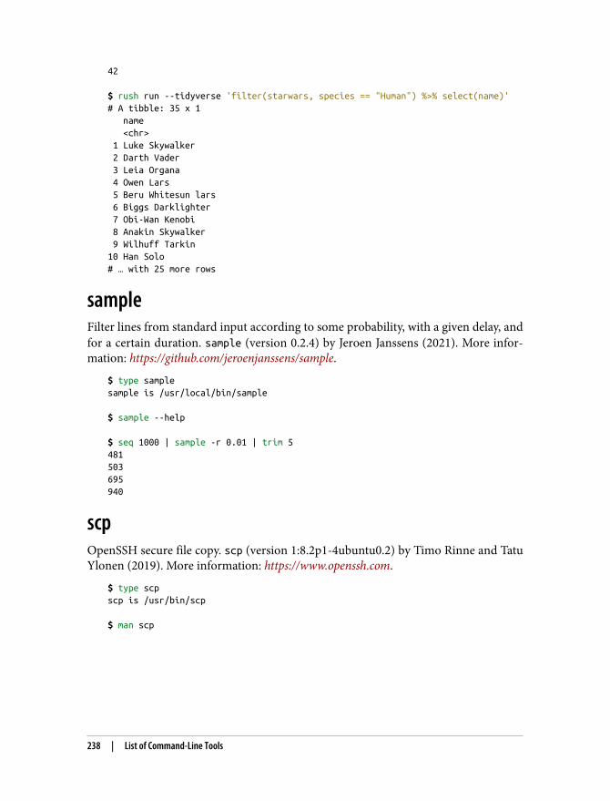
42 $ rush run --tidyverse 'filter(starwars, species == "Human") %>% select(name)'# A tibble: 35 x 1 name <chr> 1 Luke Skywalker 2 Darth Vader 3 Leia Organa 4 Owen Lars 5 Beru Whitesun lars 6 Biggs Darklighter 7 Obi-Wan Kenobi 8 Anakin Skywalker 9 Wilhuff Tarkin10 Han Solo# … with 25 more rows

sampleFilter lines from standard input according to some probability, with a given delay, andfor a certain duration. sample (version 0.2.4) by Jeroen Janssens (2021). More infor‐mation: https://github.com/jeroenjanssens/sample.

$ type samplesample is /usr/local/bin/sample $ sample --help $ seq 1000 | sample -r 0.01 | trim 5481503695940

scpOpenSSH secure file copy. scp (version 1:8.2p1-4ubuntu0.2) by Timo Rinne and TatuYlonen (2019). More information: https://www.openssh.com.

$ type scpscp is /usr/bin/scp $ man scp

238 | List of Command-Line Tools

sedStream editor for filtering and transforming text. sed (version 4.7) by Jay Fenlason,Tom Lord, Ken Pizzini, and Paolo Bonzini (2018). More information: https://www.gnu.org/software/sed.

$ type sedsed is /usr/bin/sed $ man sed

seqPrint a sequence of numbers. seq (version 8.30) by Ulrich Drepper (2019). Moreinformation: https://www.gnu.org/software/coreutils.

$ type seqseq is /usr/bin/seq $ man seq $ seq 3123 $ seq 10 5 20101520

servewdServe the current working directory using a simple HTTP server. servewd (version0.1) by Jeroen Janssens (2021). More information: https://github.com/jeroenjanssens/dsutils.

$ type servewdservewd is /usr/bin/dsutils/servewd $ servewd --help $ cd /data && servewd 8000

List of Command-Line Tools | 239

shufGenerate random permutations. shuf (version 8.30) by Paul Eggert (2019). Moreinformation: https://www.gnu.org/software/coreutils.

$ type shufshuf is /usr/bin/shuf $ man shuf $ echo {a..z} | tr ' ' '\n' | shuf | trim 5vgmzk… with 21 more lines $ shuf -i 1-100 | trim 51396685046… with 95 more lines

skllSciKit-Learn Laboratory. skll (version 2.5.0) by Educational Testing Service (2021).The actual tool is run_experiment. I use the alias skll because I find that easier toremember. More information: https://skll.readthedocs.org.

$ type skllskll is an alias for run_experiment $ skll --help

sortSort lines of text files. sort (version 8.30) by Mike Haertel and Paul Eggert (2019).More information: https://www.gnu.org/software/coreutils.

$ type sortsort is /usr/bin/sort $ man sort $ echo '3\n7\n1\n3' | sort1

240 | List of Command-Line Tools

337

splitSplit a file into pieces. split (version 8.30) by Torbjorn Granlund and Richard M.Stallman (2019). More information: https://www.gnu.org/software/coreutils.

$ type splitsplit is /usr/bin/split $ man split

spongeSoak up standard input and write to a file. sponge (version 0.65) by Colin Watson andTollef Fog Heen (2021). Useful if you want to read from and write to the same file in asingle pipeline. More information: https://joeyh.name/code/moreutils.

$ type spongesponge is /usr/bin/sponge

sql2csvExecute an SQL query on a database and output the result to a CSV file. sql2csv(version 1.0.5) by Christopher Groskopf (2020). More information: https://csvkit.rtfd.org.

$ type sql2csvsql2csv is /usr/bin/sql2csv $ sql2csv --help

sshOpenSSH remote login client. ssh (version 1:8.2p1-4ubuntu0.2) by Tatu Ylonen,Aaron Campbell, Bob Beck, Markus Friedl, Niels Provos, Theo de Raadt, and DugSong (2020). More information: https://www.openssh.com.

$ type sshssh is /usr/bin/ssh $ man ssh

List of Command-Line Tools | 241

sudoExecute a command as another user. sudo (version 1.8.31) by Todd C. Miller (2019).More information: https://www.sudo.ws.

$ type sudosudo is /usr/bin/sudo $ man sudo

tailOutput the last part of files. tail (version 8.30) by Paul Rubin, David MacKenzie, IanLance Taylor, and Jim Meyering (2019). More information: https://www.gnu.org/software/coreutils.

$ type tailtail is /usr/bin/tail $ man tail

tapkeeAn efficient dimension reduction library. tapkee (version 1.2) by Sergey Lisitsyn,Christian Widmer, and Fernando J. Iglesias Garcia (2013). More information: http://tapkee.lisitsyn.me.

$ type tapkeetapkee is /usr/bin/tapkee $ tapkee --help

tarAn archiving utility. tar (version 1.30) by John Gilmore and Jay Fenlason (2014).More information: https://www.gnu.org/software/tar.

$ type tartar is /usr/bin/tar $ man tar

teeRead from standard input and write to standard output and files. tee (version 8.30)by Mike Parker, Richard M. Stallman, and David MacKenzie (2019). More informa‐tion: https://www.gnu.org/software/coreutils.

242 | List of Command-Line Tools

$ type teetee is /usr/bin/tee $ man tee

telnetUser interface to the TELNET protocol. telnet (version 0.17) by Mats Erik Ander‐sson, Andreas Henriksson, and Christoph Biedl (1999). More information: http://www.hcs.harvard.edu/~dholland/computers/netkit.html.

$ type telnettelnet is /usr/bin/telnet

tldrCollaborative cheat sheets for console commands. tldr (version 3.3.7) by Owen Voke(2021). More information: https://tldr.sh.

$ type tldrtldr is /usr/local/bin/tldr $ tldr --help $ tldr tar | trim✔ Page not found. Updating cache...✔ Creating index... tar Archiving utility. Often combined with a compression method, such as gzip or bzip2. More information: https://www.gnu.org/software/tar. - [c]reate an archive and write it to a [f]ile: tar cf target.tar file1 file2 file3 … with 22 more lines

trTranslate or delete characters. tr (version 8.30) by Jim Meyering (2018). More infor‐mation: https://www.gnu.org/software/coreutils.

$ type trtr is /usr/bin/tr $ man tr

List of Command-Line Tools | 243

treeList contents of directories in a tree-like format. tree (version 1.8.0) by Steve Baker(2018). More information: https://launchpad.net/ubuntu/+source/tree.

$ type treetree is /usr/bin/tree $ man tree $ tree / | trim/├── bin -> usr/bin├── boot├── data│ ├── ch01│ ├── ch02│ │ ├── fac.py│ │ └── movies.txt│ ├── ch03│ │ ├── logs.tar.gz… with 122908 more lines

trimTrim output to a given height and width. trim by Jeroen Janssens (2021). More infor‐mation: https://github.com/jeroenjanssens/dsutils.

$ type trimtrim is /usr/bin/dsutils/trim $ echo {a..z}-{0..9} | fold | trim 5 60a-0 a-1 a-2 a-3 a-4 a-5 a-6 a-7 a-8 a-9 b-0 b-1 b-2 b-3 b-4…c-0 c-1 c-2 c-3 c-4 c-5 c-6 c-7 c-8 c-9 d-0 d-1 d-2 d-3 d-4…e-0 e-1 e-2 e-3 e-4 e-5 e-6 e-7 e-8 e-9 f-0 f-1 f-2 f-3 f-4…g-0 g-1 g-2 g-3 g-4 g-5 g-6 g-7 g-8 g-9 h-0 h-1 h-2 h-3 h-4…i-0 i-1 i-2 i-3 i-4 i-5 i-6 i-7 i-8 i-9 j-0 j-1 j-2 j-3 j-4…… with 8 more lines

tsTimestamp input. ts (version 0.65) by Joey Hess (2021). More information: https://joeyh.name/code/moreutils.

$ type tsts is /usr/bin/ts $ echo seq 5 | sample -d 500 | tsJun 29 14:39:19 seq 5

244 | List of Command-Line Tools

typeShow the type and location of a command-line tool. type is a Z shell builtin.

$ type typetype is a shell builtin $ man zshbuiltins | grep -A 10 '^ *type '

uniqReport or omit repeated lines. uniq (version 8.30) by Richard M. Stallman and DavidMacKenzie (2019). More information: https://www.gnu.org/software/coreutils.

$ type uniquniq is /usr/bin/uniq $ man uniq

unpackExtract common file formats. unpack (version 0.1) by Patrick Brisbin (2013). Moreinformation: https://github.com/jeroenjanssens/dsutils.

$ type unpackunpack is /usr/bin/dsutils/unpack

unrarExtract files from RAR archives. unrar (version 0.0.1) by Ben Asselstine, ChristianScheurer, and Johannes Winkelmann (2014). More information: https://web.archive.org/web/20080331080828/http://home.gna.org/unrar/.

$ type unrarunrar is /usr/bin/unrar $ man unrar

unzipList, test, and extract compressed files in a ZIP archive. unzip (version 6.0) by SamuelH. Smith, Ed Gordon, Christian Spieler, Onno van der Linden, Mike White, Kai UweRommel, Steven M. Schweda, Paul Kienitz, Chris Herborth, Jonathan Hudson, SergioMonesi, Harald Denker, John Bush, Hunter Goatley, Steve Salisbury, Steve Miller, andDave Smith (2009). More information: http://www.info-zip.org/pub/infozip.

$ type unzipunzip is /usr/bin/unzip

List of Command-Line Tools | 245

$ man unzip

vwFast machine learning library for online learning. vw (version 8.10.1) by John Lang‐ford (2021). More information: https://vowpalwabbit.org.

$ type vwvw is /usr/local/bin/vw $ vw --help --quiet

wcPrint newline, word, and byte counts for each file. wc (version 8.30) by Paul Rubinand David MacKenzie (2019). More information: https://www.gnu.org/software/coreutils.

$ type wcwc is /usr/bin/wc $ man wc

whichLocate a command. which (version 0.1) by unknown (2016).

$ type whichwhich is a shell builtin $ man which

xml2jsonConvert an XML input to a JSON output, using xml-mapping. xml2json (version0.0.3) by François Parmentier (2016). More information: https://github.com/parmentf/xml2json.

$ type xml2jsonxml2json is /usr/local/bin/xml2json

xmlstarletCommand-line XML/XSLT toolkit. xmlstarlet (version 1.6.1) by Dagobert Michel‐sen, Noam Postavsky, and Mikhail Grushinskiy (2019). More information: https://sourceforge.net/projects/xmlstar.

246 | List of Command-Line Tools

$ type xmlstarletxmlstarlet is /usr/bin/xmlstarlet $ man xmlstarlet

xsvA fast CSV command-line toolkit written in Rust. xsv (version 0.13.0) by AndrewGallant (2018). More information: https://github.com/BurntSushi/xsv.

$ type xsvxsv is /usr/bin/xsv $ xsv --help

zcatDecompress and concatenate files to standard output. zcat (version 1.10) by PaulEggert (2021). More information: https://www.nongnu.org/zutils/zutils.html.

$ type zcatzcat is /usr/bin/zcat $ man zcat

zshThe Z shell. zsh (version 5.8) by Paul Falstad and Peter Stephenson (2020). Moreinformation: https://www.zsh.org.

$ type zshzsh is /usr/bin/zsh $ man zsh

List of Command-Line Tools | 247

Index

Symbols$ (dollar sign) prompt, 14, 111$@ variable, 113

Aadvice, 214-215algorithms

modeling data, 177classification, 177, 193-197dimensionality reduction, 177, 182-187regression, 177, 187-192

alias tool, 219aliases, 19Apache Spark, 208-210arguments, one-liner conversion to shell script,

66-67as_tibble( ) function, 184authentication, web APIs, 48-49automatic variables, 113awk tool, 80, 96, 220AWS EC2, running instances, 167-168aws tool, 168, 220

Bbar charts, 140-141bash command-line tool, 60bash magic, 203Bash shell, 116bash tool, 62-67, 220bat tool, 29, 220bc tool, 155, 166, 221binary executables, 17body tool, 90-92, 221box plots, 114, 149-150

brace expansion, 155

Ccat tool, 121, 221categorical variables, 124-126cd tool, 15, 17, 222characters, deleting, 89chmod tool, 61, 222classification, 177classification models, 193-197classifiers

results, 195-197skll tool, 193, 194

code, converting to command-line tool, 8cols tool, 90, 92, 97, 222column tool, 29, 222columns

CSV filesextracting and reordering, 94-95merging, 96-98

data types, 123headers, 122

comma-separated values (CSV) (see CSV(comma-separated values))

commandunpack, 42

command lineagility, 7as augmenting technology, 8extensibility, 9filesystem and, 8languages, 9prompt, 7, 14REPL (read-eval-print loop), 7

249

scalability, 8shell, 6terminal, 6ubiquity, 9

command-line toolsalias, 19, 219arguments, 66awk, 80, 96, 220aws, 168, 220bash, 62-67, 220bat, 29, 220bc, 155, 166, 221binary executables, 17body, 90-92, 221cat, 121, 221cd, 15, 17, 222chmod, 61, 222cols, 90, 92, 97, 222column, 29, 222combining, 20-22communication streams, 20converting from code, 8cowsay, 12, 162, 223cp, 27, 223creating, 4csv2vw, 187, 223csvcut, 122, 223csvgrep, 46, 95, 124, 224csvjoin, 100, 224csvlook, 29, 44, 123, 224csvquote, 225csvsort, 124, 225csvsql, 96, 98, 225csvstack, 180, 225csvstat, 126-129, 226curl, 37-38, 65, 226cut, 87, 94, 226display, 133, 226docker, 12dseq, 25, 227echo, 23, 61, 227env, 64, 227export, 228fc, 58, 228find, 157, 228fold, 29, 228for, 229fx, 229git, 108, 229

gluing, 8GNU Parallel, 5grep, 20, 79, 84, 87, 230gron, 230head, 82, 122-124, 230header, 90, 91, 230history, 231hostname, 231in2csv, 43, 231interpreted scripts, 17jq, 101, 104, 231json2csv, 101, 232l, 19, 232less, 121, 232ls, 26, 233make, 5, 108, 233man, 30, 233mkdir, 27, 233mv, 27, 234nano, 234nl, 121, 234parallel, 154, 155, 160-162, 234paste, 99, 235PATH variable, 68-69pbc, 166, 235pip, 202, 235pup, 103, 236pwd, 15, 17, 20, 236python, 70, 236R, 237rev, 20, 237rm, 27, 237Rscript, 70run_experiment, 193rush, 80, 129-133, 183, 237rush plot, 138, 191sample, 85, 238scp, 238sed, 82, 84, 89, 96, 239seq, 14, 18, 110, 239servewd, 137, 239shell builtins, 17shell functions, 18shuf, 188, 240skll, 178, 193, 194-195, 240sort, 79, 240split, 188, 241sponge, 25, 241sql2csv, 46, 241

250 | Index

ssh, 241sudo, 28, 242syntax shortcuts, 142tail, 82, 242tapkee, 183, 242tar, 41, 242tee, 99, 242telnet, 51, 243tldr, 32, 243tr, 88, 122-124, 180tree, 244trim, 28, 121, 244ts, 86, 244type, 19, 245uniq, 79, 245Unix, 14, 15-16unpack, 245unrar, 41, 245unzip, 41, 245vw, 246wc, 22-24, 246which, 246xml2json, 101, 103, 246xmlstarlet, 246xsv, 129, 247zcat, 171, 247zsh, 17, 247

communication streams, 20compressed files, decompressing, 41-42concurrent jobs, parallel processing, 164confusion matrix, 196cowsay tool, 12, 162, 223cp tool, 27, 223creativity, 215CSV (comma-separated values)

bodies, 90-93columns, 90-93

extracting and reordering, 94-95merging, 96-98

concatenating files, 99csvcut tool, 122files, 174

combining, 99-100converting Excel to, 43-46headers, 44, 45joining, 100

headers, 90-93line breaks, 43rows, filtering, 95-96

SQL queries, 93-93csv2vw tool, 187, 223csvcut tool, 122, 223csvgrep tool, 46, 95, 124, 224csvjoin tool, 100, 224csvlook tool, 29, 44, 123, 224csvquote tool, 225csvsort tool, 124, 225csvsql tool, 96, 98, 225csvstack tool, 180, 225csvstat tool, 126-129, 226curl tool, 37-38, 65, 226

file saving, 38output, 21redirects, 39

curly braces, 156cut tool, 87, 94, 226

Ddata points, 177

features, 177Labels, 177

data properties, 120-126data types, 122-124data visualization

bar charts, 140-141box plots, 149-150density plots, 143-144, 181ggplot2, 138-140graphical, 139histograms, 142-142images, 133-138labels, 150-152rush tool and, 138-140scatter plots, 146-146textual, 139trend lines, 147-148

databases, relational, 46-47datasets, 177

creating, 88downloading, 11files, combining, 180values, missing, 180wine dataset, 178

decompressing files, 41-42density plots, 143-144, 181dependencies (Makefiles), 113-118descriptive statistics, 126-133DICT protocol, 39

Index | 251

dictionaries, 39dimensionality reduction, 177

Tapkee, 182-187directories

creating, 27listing, 68listing contents, 26moving, 27removing, 27renaming, 27volumes, 13

display tool, 133, 226distributed processing, 167

AWS EC2 instances, 167-168local data on remote machines, 170-171remote machines, 169remote machines, file processing, 171-174

Dockercontainers, 12

volumes, 13downloading, 12images

installation, 6, 12-13running, 12

docker tool, 12dollar sign ($), 7downloads

datasets, 11files, 37-40

curl tool, 37FTP server, 39

dseq tool, 25, 227

Eecho tool, 23, 61, 227env tool, 64, 227Excel spreadsheets, converting to CSV files,

43-46exploring data, 3

data visualizations, 133-152descripting statistics, 126-133inspecting, 120-126properties, 120-126

export tool, 228extensibility, 9

Ffac function, 18factor( ) function, 149

fc builtin, 58, 228feature names, 122-124fifo( ) function, 205file extensions

.sh (shell scripts), 60compressed files, 41.make, 109

File Transfer Protocol (FTP), 39-40files

copying, 27to Docker container, 36

creating, 27CSV files, combining, 99-100decompressing, 41-42downloading, 37-40

curl tool, 37FTP server, 39

moving, 27naming, 58renaming, 27saving, 38text editor, 58visual file managers, 28

filesystem, 8filtering rows, CSV files, 95-96find tool, 157, 228fixed input, one-liner conversion to shell script,

65-66fold tool, 29, 228for loops, 155for tool, 229FTP (File Transfer Protocol), 39-40functions

as_tibble( ), 184fac, 18factor( ), 149fifo( ), 205geom_bar, 144geom_density, 144geom_histogram, 144pipe( ), 205, 210Python, 73qplot, 139R, 73scale( ), 184sh( ), 206shell functions, 18system2( ), 205

fx tool, 229

252 | Index

Ggeom_bar function, 144geom_density function, 144geom_histogram function, 144ggplot2, 138-140git tool, 108, 229GitHub, 108globbing, 157GNU Midnight Commander, 28GNU Parallel, 5, 160-162graphical user interface (GUI) (see GUI (graph‐

ical user interface))graphical visualization, 139grep tool, 20, 79, 84, 87, 206, 230

output, 21stopwords, filtering, 57

gron tool, 230GUI (graphical user interface), 6

Docker GUI, 12versus command line, 8

Hhead tool, 82, 122-124, 230header tool, 90, 91, 230headers

checking for, 120-121column names, 122

help, man tool, 30histograms, 142-142history tool, 231hostname tool, 231HTML files, downloading, 102

Iimages

data visualization and, 133-138displaying

as text, 134-136manually open, 136-137open in browser, 137-138terminal, 134-136

inserting, 30in2csv tool, 43, 231input

fixed, removing, 65-66parallel processing, 162-163redirecting, 22-26streaming data processing, 72-74

tool output, 21inspecting data, 120-126intermediate output, 30interpreted scripts, 17interpreting data, 4iTerm2 terminal, 136

Jjoining CSV files, 100jq tool, 101, 104, 231JSON

confusion matrix, 196EC2 instances, 168file transfer to remote machine, 173head tool, 172objects, flattening, 171scrubbing data and, 101-104

json2csv tool, 101, 232Jupyter, 200-203Jupyter Console, 200-202Jupyter Notebook, 202JupyterLab, 202

Ll tool, 19, 232Labels, data points, 177less tool, 121, 232line filtering

by location, 81-84by pattern, 84-85by randomness, 85-86

line numbers, 121looping

for loops, 155over files, 157over lines, 156-157over numbers, 155while loops, 156

ls tool, 26, 233remote machines, 174

M.make file extension, 109make tool, 5, 108-109, 233

$ (dollar) sign, 111command execution and, 109soft tabs, 110source code compile, 111

Index | 253

targets, building, 110Makefile, 109

box plots, 114dependencies, 113-118ONESHELL variable, 116PHONY variable, 116rules, 110

writing output to file, 112-113sh (shell), 116SHELL variable, 116SHELLFLAGS variable, 116syntax, 115targets, 110

all, 117building, 110, 112-113data, 117data/starwars.csv, 117heights.png, 117phony, 111, 116top10, 117

tasks, running, 109-112URL variable, 116whitespace, 110

man pages, 57man tool, 30, 233merging columns, CSV files, 96-98mkdir tool, 27, 233modeling data, 4

algorithms, 177classification, 177, 193-197dimensionality reduction, 177, 182-187regression, 177, 187-192

mv tool, 27, 234MySQL, 46

Nnano tool, 234nl tool, 121, 234

Oobtaining data, 3

copying files, Docker container, 36downloading files, 37-40relational databases, 46-47web APIs, 47-51

one-liners, 53converting to shell scripts, 55-69

arguments, 66-67execute permission, 61-62

file creation, 58-61fixed input removal, 65-66PATH variable, 68-69shebang, 62-64

R and, 129-133rush tool and, 131

OSEMN model, 2, 213(see also specific steps)exploring data, 3interpreting data, 4modeling data, 4obtaining data, 3scrubbing data, 3

outputintermediate, 30limiting, 28management, 28-30parallel processing and, 164-165redirecting, 22-26saving to file, 23suppressing, 24

Pparallel processing, 158-159

concurrent jobs, 164input specification, 162-163logging, 164-165output, 164-165parallel tool, 160-162parallel tools, creating, 166

parallel tool, 154, 160-162, 234concurrent jobs, 164looping

over files, 157over lines, 156-157over numbers, 155

triple colon, 179paste tool, 99, 235PATH variable, one-liner conversion to shell

script, 68-69patience, 214pbc tool, 166, 235permissions, one-liner conversion to shell

script, 61-62phony targets, 111pip tool, 202, 235pipe( ) function, 205, 210pipelines, 53plain text, scrubbing data and, 81-90

254 | Index

polygot definition, 199porting shell scripts, 70-72PostgreSQL, 46practicality, 215prompt, 7, 14pup tool, 103, 236pwd tool, 15, 17, 20, 236Python, 203-204

command-line toolscreating, 69-74

subprocess module, 203python tool, 70, 236

Qqueries, CSV files, 93-93

RR, 205-206

command-line tools, creating, 69-74one-liners, 129-133REPL (read-eval-print loop), 129

R tool, 237Ranger file manager, 28redirects, curl tool, 39regression, 177

model testing, 190-192model training, 188-190predictions, 190vw (Vowpal Wabbit), 187-192

regular expressionssed tool, 89syntax, 45

relational databases, queries, 46-47remote machines

file processing, 171-174local data distribution, 170-171ls tool, 174running commands, 169

renaming files, mv tool, 27REPL (read-eval-print loop), 7, 129resources, 215rev tool, 20, 237rm tool, 27, 237rows, CSV files, filtering, 95-96Rscript tool, 70RStudio, 207rules (Makefiles), 110

output, writing to file, 112-113shell and, 116

run subcommand, 131run_experiment tool, 193

skll tool, 193rush plot tool, 138, 191

geometry, 143plotting options, 139-140qplot function, 139saving options, 139-140stacked histogram, 142

rush tool, 80, 129-133, 183, 237

Ssample tool, 85, 238saving files, curl tool, 38scalability, 8scale( ) function, 184scatter plots, 146-146scp tool, 238scripts

interpreted, 17shell

converting from one-liners, 55-69one-liners as, 54porting, 70-72

shells and, 18scrubbing data, 3

CSVbodies, 90-93columns, 90-93, 94-95, 96-98combining files, 99-100headers, 90-93rows, 95-96SQL queries, 93-93

filtering linesby location, 81-84by pattern, 84-85by randomness, 85-86

JSON files and, 101-104plain text and, 81-90values

deleting, 88-90extracting, 86-88replacing, 88-90

XML/HTML files and, 101-104sed tool, 82, 84, 89, 96, 239

combining commands, 90seq tool, 14, 18, 110, 239serial processing, looping

over files, 157

Index | 255

over lines, 156-157over numbers, 155

servewd tool, 137, 239.sh file extension, 60sh( ) function, 206shebang, one-liner conversion to shell script,

62-64shell, 6

Bash, 116parentheses, 163quotes in, 163rule execution, 116Unix, 14Z shell, 14

shell builtins, 17shell functions, 18shell scripts, 18

converting from one-liners, 55-69arguments, 66-67execute permission, 61-62file creation, 58-61fixed input, 65-66PATH variable, 68-69shebang, 62-64

one-liners as, 54porting, 70-72.sh file extension, 60

shuf tool, 188, 240SKLL (SciKit-Learn Laboratory), 193-197skll tool, 178, 193, 240

classifiers, files, 196running experiment, 194

soft tabs, 110sort tool, 79, 240special characters, 157split tool, 188, 241sponge tool, 25, 241SQL queries, CSV files, 93-93sql2csv tool, 46, 241SQLite, 46SSH (Secure Shell), 167ssh tool, 241stacked histogram, 142statistics, descriptive, 126-133stderr, 20stdin, 20stdout, 20stopwords, 56streaming

APIs, 49-51data processing, 72-74

subprocess module (Python), 203sudo tool, 28, 242syntax

Makefile, 115regular expressions, 45rush, 138shortcuts, 142

system2( ) function, 205

Tt-SNE, 186tail tool, 82, 242Tapkee, 182

mappings, 183-187tapkee tool, 242tar tool, 41, 242tar.gz files, 41targets (Makefiles), 110

all, 117building, 110

writing output to file, 112-113data, 117data/starwars.csv, 117heights.png, 117phony, 111, 116top10, 117

tasks, Makefile, 109-112tee tool, 99, 242telnet tool, 51, 243terminal, 6

Unix, 14text editor, fc builtin, 58textual visualization, 139tidyverse, 183timestamps, 86tldr tool, 32, 243tools, 4

(see also command-line tools)tr tool, 88, 122-124, 180transformations, 78tree tool, 244trend lines, data visualization and, 147-148trim tool, 28, 121, 244ts tool, 86, 244type tool, 19, 245

256 | Index

UUbuntu, 5uniq tool, 79, 245unique identifiers, 124

unique values and, 124-126Unix, 15

command-line tools, 14executing, 15

directories, 16prompt, 14shell, 14terminal, 14

unpack tool, 42, 245unrar tool, 41, 245unzip tool, 41, 245

Vvalues

datasets, missing, 180deleting, 88-90extracting, 86-88replacing, 88-90unique identifiers and, 124-126

variablesautomatic, 113categorical, 124-126

version control, 108GitHub, 108

Vifm file manager, 28

vw (Vowpal Wabbit), 187-192csv2vw tool, 187options, 188

vw tool, 187-192, 246

Wwc tool, 22-24, 246web APIs, 47-51

authentication, 48-49which tool, 246while loops, 156whitespace, 110wine dataset, 178workflow, 109

(see also make tool)

XXML/HTML files, scrubbing data and, 101-104xml2json tool, 101, 103, 246xmlstarlet tool, 246xsv tool, 129, 247

ZZ shell, 14

(see also shell)zcat tool, 171, 247zsh tool, 17, 247

Index | 257

About the AuthorJeroen Janssens is an independent data science consultant and instructor. He enjoysvisualizing data, implementing machine learning models, and building solutionsusing Python, R, JavaScript, and Bash. Jeroen manages Data Science Workshops, atraining and coaching firm that organizes open enrollment workshops, in-companycourses, inspiration sessions, hackathons, and meetups. Previously, he was an assis‐tant professor at Jheronimus Academy of Data Science and a data scientist at Elsevierin Amsterdam and various startups in New York City. Jeroen holds a PhD in machinelearning from Tilburg University and an MSc in artificial intelligence from MaastrichtUniversity. He lives with his wife and two kids in Rotterdam, the Netherlands.

ColophonThe animal on the cover of Data Science at the Command Line is a wreathed hornbill(Rhytidoceros undulatus). Also known as the bar-pouched wreathed hornbill, the spe‐cies is found in forests in mainland Southeast Asia and in northeastern India andBhutan. Hornbills are named for the casques that form on the upper part of the birds’bills. No single obvious purpose exists for these hollow, keratizined structures, butthey may serve as a means of recognition between members of the species, as anamplifier for the birds’ calls, or—because males often exhibit larger casques thanfemales of the species—for gender recognition. Wreathed hornbills can be distin‐guished from plain-pouched hornbills, to whom they are closely related and other‐wise similar in appearance, by a dark bar on the lower part of the wreathed hornbills’throats.

Wreathed hornbills roost in flocks of up to four hundred but mate in monogamous,lifelong partnerships. With help from the males, females seal themselves up in treecavities behind dung and mud to lay eggs and brood. Through a slit large enough forhis beak alone, the male feeds his mate and their young for up to four months. A dietof animal prey becomes predominantly fruit when females and their young leave thenest. Hornbill couples have been known to return to the same nest for as many asnine years.

Many of the animals on O’Reilly covers are endangered; all of them are important tothe world.

The color illustration is by Karen Montgomery, based on a black and white engravingfrom Braukhaus’s Lexicon. The cover fonts are Gilroy Semibold and Guardian Sans.The text font is Adobe Minion Pro; the heading font is Adobe Myriad Condensed;and the code font is Dalton Maag’s Ubuntu Mono.

There’s much more where this came from.Experience books, videos, live online training courses, and more from O’Reilly and our 200+ partners—all in one place.

Learn more at oreilly.com/online-learning

©20

19 O

’Rei

lly M

edia

, Inc

. O’R

eilly

is a

regi

ster

ed tr

adem

ark

of O

’Rei

lly M

edia

, Inc

. | 17

5