Deafening Mosquitoes and Underwater Ranging

© Copyright by Praveen Kumar Reddy Padala 2018

All Rights Reserved

Sensing Technologies for Mosquito Control:

Deafening Mosquitoes and Underwater Ranging

A Thesis

Presented to

the Faculty of the Department of Electrical and Computer Engineering

University of Houston

in Partial Fulfillment

of the Requirements for the Degree

Master of Science

in Electrical Engineering

by

Praveen Kumar Reddy Padala

December 2018




Approved:

Chairman of the Committee

Aaron T. Becker, Assistant Professor,

Department of Electrical and Computer

Engineering

Committee Members

David R. Jackson, Professor,

Department of Electrical and Computer

Engineering

Ricardo Lent, Associate Professor, Department of Computer Engineering

Technology

Suresh K. Khator, Associate Dean, Badrinath Roysam, Professor, Chair, Cullen College of Engineering Electrical and Computer Engineering

v

Acknowledgments

I would like to thank my advisor, Dr. Aaron T.Becker for being a great advisor and

also a good human being with values. Thank you, Dr. David Jackson and Dr. Ricardo Lent,

for being a part of my thesis committee. I would like to thank Dr. Debboun, Chris, Pamela,

Jude, John, Elaine, Allison and Sammy for all your invaluable support when I performed

the deafening mosquito experiments at the Harris County Mosquito and Vector Control

division. Thank you also to Mr. William Hamby III for sharing your insights on the speaker

design and many other things. Thank you, Mr. Victor Gallardo for your continued support

and for also being flexible at times with my TA job responsibilities. A special thanks to my

dear friends Anirudh, Prashant, Satish, Jisnu and Sumit for watching my back all the time.

Most of all, I would like to thank my parents and my sister without whom this journey

would not be possible.

vi



An Abstract

of a Thesis

Presented to

the Faculty of the Department of Electrical and Computer Engineering

University of Houston

in Partial Fulfillment

of the Requirements for the Degree Master of Science

in Electrical and Computer Engineering

by


December 2018

vii

Abstract

This thesis is comprised of two projects related to mosquito sensing technologies.

In the first project, a novel method is proposed in which sound waves with high particle

velocities are used to potentially disrupt the mating process in mosquitoes. The

experimental setup and the results are elucidated in this thesis. The second project is about

the design of an underwater depth finding sensor module which is used in an autonomous

remote operated vehicle developed by the Robotic Swarm Control Lab to kill mosquito

larvae in water bodies. The analog circuit design and the embedded programming are

shown in this thesis.

viii

Table of Contents

Acknowledgments. . . . . . . . . . . . . . . . . . . . . . . . . . . . . . . . . . . . . . . . . . . . . . . . . . . . . . v

Abstract. . . . . . . . . . . . . . . . . . . . . . . . . . . . . . . . . . . . . . . . . . . . . . . . . . . . . . . . . . . . . vii

Table of Contents. . . . . . . . . . . . . . . . . . . . . . . . . . . . . . . . . . . . . . . . . . . . . . . . . . . . . viii

List of Figures. . . . . . . . . . . . . . . . . . . . . . . . . . . . . . . . . . . . . . . . . . . . . . . . . . . . . . . . . x

List of Tables. . . . . . . . . . . . . . . . . . . . . . . . . . . . . . . . . . . . . . . . . . . . . . . . . . . . . . . . . xii

List of Samples. . . . . . . . . . . . . . . . . . . . . . . . . . . . . . . . . . . . . . . . . . . . . . . . . . . . . . . xiii

1 Deafening Mosquitoes. . . . . . . . . . . . . . . . . . . . . . . . . . . . . . . . . . . . . . . . . . . . . . . . .1

1.1 Importance of Sound in the Mosquito Mating Process. . . . . . . . . . . . . . . . . . . . . . . 1

1.2 Experimental Setup. . . . . . . . . . . . . . . . . . . . . . . . . . . . . . . . . . . . . . . . . . . . . . . . . . 2

1.2.1 Design Calculations. . . . . . . . . . . . . . . . . . . . . . . . . . . . . . . . . . . . . . . . . . . . 5

1.2.2 Variant-1. . . . . . . . . . . . . . . . . . . . . . . . . . . . . . . . . . . . . . . . . . . . . . . . . . . . .8

1.2.3 Variant-2. . . . . . . . . . . . . . . . . . . . . . . . . . . . . . . . . . . . . . . . . . . . . . . . . . . . .9

1.3 Results and Analysis. . . . . . . . . . . . . . . . . . . . . . . . . . . . . . . . . . . . . . . . . . . . . . . . 11

1.4 Limitations of the Experimental Setup. . . . . . . . . . . . . . . . . . . . . . . . . . . . . . . . . . 12

1.5 Future Work. . . . . . . . . . . . . . . . . . . . . . . . . . . . . . . . . . . . . . . . . . . . . . . . . . . . . . .13

2 Underwater Ranging. . . . . . . . . . . . . . . . . . . . . . . . . . . . . . . . . . . . . . . . . . . . . . . . .15

2.1 Problem Statement. . . . . . . . . . . . . . . . . . . . . . . . . . . . . . . . . . . . . . . . . . . . . . . . . .15

2.2 Working Principle. . . . . . . . . . . . . . . . . . . . . . . . . . . . . . . . . . . . . . . . . . . . . . . . . . 16

2.3 Ultrasonic Transducer Calculations. . . . . . . . . . . . . . . . . . . . . . . . . . . . . . . . . . . . .17

2.4 Analog Circuit Design. . . . . . . . . . . . . . . . . . . . . . . . . . . . . . . . . . . . . . . . . . . . . . .20

ix

2.4.1 Choosing a suitable Op-Amp. . . . . . . . . . . . . . . . . . . . . . . . . . . . . . . . . . . . .23

2.4.2 Clipper Circuit. . . . . . . . . . . . . . . . . . . . . . . . . . . . . . . . . . . . . . . . . . . . . . . . 24

2.4.3 Unity Gain Buffer-Stability. . . . . . . . . . . . . . . . . . . . . . . . . . . . . . . . . . . . . . 25

2.4.4 Peak Detector. . . . . . . . . . . . . . . . . . . . . . . . . . . . . . . . . . . . . . . . . . . . . . . . .26

2.4.5 Comparator-1. . . . . . . . . . . . . . . . . . . . . . . . . . . . . . . . . . . . . . . . . . . . . . . . .27

2.4.6 Comparator-2. . . . . . . . . . . . . . . . . . . . . . . . . . . . . . . . . . . . . . . . . . . . . . . . .28

2.5 Embedded System. . . . . . . . . . . . . . . . . . . . . . . . . . . . . . . . . . . . . . . . . . . . . . . . . . 29

2.5.1 Edge Triggered Interrupts. . . . . . . . . . . . . . . . . . . . . . . . . . . . . . . . . . . . . . . 29

2.5.2 Systick Timer and Interrupt. . . . . . . . . . . . . . . . . . . . . . . . . . . . . . . . . . . . . .30

2.5.2 Flowcharts. . . . . . . . . . . . . . . . . . . . . . . . . . . . . . . . . . . . . . . . . . . . . . . . . . . 31

2.6 Results. . . . . . . . . . . . . . . . . . . . . . . . . . . . . . . . . . . . . . . . . . . . . . . . . . . . . . . . . . . 36

2.7 Future Work. . . . . . . . . . . . . . . . . . . . . . . . . . . . . . . . . . . . . . . . . . . . . . . . . . . . . . .36

3 Conclusion. . . . . . . . . . . . . . . . . . . . . . . . . . . . . . . . . . . . . . . . . . . . . . . . . . . . . . . . . 37

References. . . . . . . . . . . . . . . . . . . . . . . . . . . . . . . . . . . . . . . . . . . . . . . . . . . . . . . . . . . .38

x

List of Figures

Figure 1.1 Comparison of female antenna (left) and male antenna (right) [1] . . . . . . . . . .1

Figure 1.2 Frequency responses for the A, B, and C-weighting networks [4] . . . . . . . . . . .4

Figure 1.3 Sound level meter indicating 130 dB . . . . . . . . . . . . . . . . . . . . . . . . . . . . . . . . 6

Figure 1.4 Frequency response of the Orion HCCA104NHP speaker [5] . . . . . . . . . . . . . .7

Figure 1.5 Male mosquitoes glued to pinheads. . . . . . . . . . . . . . . . . . . . . . . . . . . . . . . . . . 8

Figure 1.6 Setup of the glass plate method [6] . . . . . . . . . . . . . . . . . . . . . . . . . . . . . . . . . .10

Figure 1.7 Mosquitoes in transfer cups. . . . . . . . . . . . . . . . . . . . . . . . . . . . . . . . . . . . . . . . 11

Figure 1.8 Mosquito pupae for the big cages (left) and small cages (right) . . . . . . . . . . . .12

Figure 1.9 Specifications (left), SPL vs distance (right) of LRAD-100 [9]. . . . . . . . . . . . .14

Figure 2.1 Larvasonic© Remotely Operated Vehicle (ROV) [10] . . . . . . . . . . . . . . . . . . .15

Figure 2.2 Specifications of an Airmar 235KHz-A transducer [13] . . . . . . . . . . . . . . . . . .17

Figure 2.3 Circuit diagram and simulation of the driver and feedback circuit . . . . . . . . . .20

Figure 2.4 A Gobing portable and wireless fish and depth finder [19] . . . . . . . . . . . . . . . .21

Figure 2.5 Venterior VT-FF001 fish finder with a wired ultrasonic transducer [20] . . . . .21

Figure 2.6 20 sine pulses generated by the Venterior fish finder . . . . . . . . . . . . . . . . . . . .22

Figure 2.7 System level block diagram. . . . . . . . . . . . . . . . . . . . . . . . . . . . . . . . . . . . . . . 22

Figure 2.8 Complete analog circuit. . . . . . . . . . . . . . . . . . . . . . . . . . . . . . . . . . . . . . . . . . .23

Figure 2.9 Clipper stage input(yellow) vs output(blue) waveforms. . . . . . . . . . . . . . . . . .24

Figure 2.10 LF 411 Op-amp internal schematic [22] . . . . . . . . . . . . . . . . . . . . . . . . . . . . .25

Figure 2.11 Open-loop gain vs phase margin with an RC load [22] . . . . . . . . . . . . . . . . . .26

xi

Figure 2.12 Peak detector circuit with output waveform (blue). . . . . . . . . . . . . . . . . . . . . 27

Figure 2.13 Comparator-1 output waveform, waveform at the transducer. . . . . . . . . . . . .27

Figure 2.14 Comparator-2 output waveform, waveform at the transducer. . . . . . . . . . . . .28

Figure 2.15 Systick handler flow chart. . . . . . . . . . . . . . . . . . . . . . . . . . . . . . . . . . . . . . . .32

Figure 2.16 Flow chart of the main program. . . . . . . . . . . . . . . . . . . . . . . . . . . . . . . . . . . 32

Figure 2.17 Flow chart of the GPIO PORTF handler. . . . . . . . . . . . . . . . . . . . . . . . . . . . . 34

Figure 2.18 High voltage pulses with peak values closer to echoes. . . . . . . . . . . . . . . . . . 35

xii

List of Tables

Table 1.1 Conversion of sound levels from flat response to A, B, C Weightings. . . . . . . .5

Table 2.1 Registers of the Systick timer. . . . . . . . . . . . . . . . . . . . . . . . . . . . . . . . . . . . . . . . . 30

xiii

List of Samples

α: absorption of sound in seawater.

c: speed of sound.

d: calculated depth.

DI: transducer directivity.

Lp: loudness.

NL: noise level.

𝒑𝒓𝒎𝒔: root-mean-square sound pressure.

p: instantaneous pressure.

ρ: quiescent density of air.

p: instantaneous sound pressure.

r: depth to seabed.

RVR: receiver efficiency of the ultrasonic transducer.

S: salinity.

SL: source level.

SR: slew rate.

t: temperature.

τ: time interval of measurement.

T: time elapsed.

TL: transmission loss.

TS: target strength.

xiv

TVR: transmission efficiency of the ultrasonic transducer.

𝑳𝑺

𝑵

: signal to noise ratio.

u: particle velocity.

Vecho: voltage (r.m.s.) due to echo.

Vin: input voltage (r.m.s.).

z: maximum depth.

1

Chapter 1

Deafening Mosquitoes

This chapter tests the hypothesis that 130 dB noise can prevent mosquitoes from

mating by deafening them. Though the results obtained from the experiments were

inconclusive, this chapter explains the methodology and theory.

1.1 Importance of Sound in the Mosquito Mating process

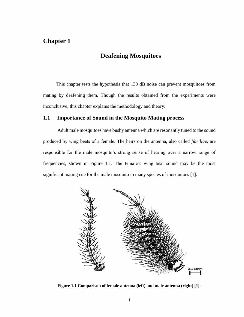
Adult male mosquitoes have bushy antenna which are resonantly tuned to the sound

produced by wing beats of a female. The hairs on the antenna, also called fibrillae, are

responsible for the male mosquito’s strong sense of hearing over a narrow range of

frequencies, shown in Figure 1.1. The female’s wing beat sound may be the most

significant mating cue for the male mosquito in many species of mosquitoes [1].

Figure 1.1 Comparison of female antenna (left) and male antenna (right) [1].

2

It has been established in the literature that the antenna of the male mosquito

responds to the particle velocity component of female’s wingbeat sound and vibrates in X,

Y, Z directions which results in the mechanical receptors lying at the base of the antenna

to either stretch or compress in tandem with sound resulting in the production of sound

evoked potentials which are electrical signals corresponding to the sound [2].

Consequently, a male mosquito mates with an aerial female but does not seem to

respond to or sense a resting female. Recently emerged males are often quickly seized by

older males because the sound produced by the young male in flight falls within the sound

spectrum which stimulates a sexually active male to copulate. Older males cannot

differentiate between the sex of young males and several-hours-old females [3].

Based on the premise that the male mosquitoes heavily rely on the hearing process

to mate with a female, we hypothesize that deafening mosquitoes will prevent them from

mating. We propose an experimental setup to investigate the effects of sound waves with

high particle velocities and frequencies ranging from 250 – 650 Hz on the hearing process

of the male mosquitoes.

The end goal is to investigate whether deafening male mosquitoes with sound

incapacitates their ability to find a female mosquito. This approach also relies on the mating

behavior of male mosquitoes in many species wherein each male constantly seek a female

partner and it is not the other way around. The reason for choosing the above-mentioned

frequencies is that the female wing beat sounds of many species of mosquitoes fall in this

frequency range.

1.2 Experimental Setup

Before proceeding to the experimental setup, key terms and definitions relevant to

3

the thesis are introduced in this section.

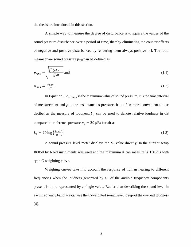
A simple way to measure the degree of disturbance is to square the values of the

sound pressure disturbance over a period of time, thereby eliminating the counter-effects

of negative and positive disturbances by rendering them always positive [4]. The root-

mean-square sound pressure prms can be defined as

𝑝𝑟𝑚𝑠 = √∫ ((𝑝2 )𝑑𝑡 )

𝜏0

∫ 𝑑𝑡𝜏

0

and (1.1)

𝑝𝑟𝑚𝑠 = 𝑝𝑚𝑎𝑥

√2 . (1.2)

In Equation 1.2, 𝑝𝑚𝑎𝑥 is the maximum value of sound pressure, τ is the time interval

of measurement and p is the instantaneous pressure. It is often more convenient to use

decibel as the measure of loudness. 𝐿𝑝 can be used to denote relative loudness in dB

compared to reference pressure 𝑝0 = 20 µPa for air as

𝐿𝑝 = 20 log (𝑝𝑟𝑚𝑠

𝑝0). (1.3)

A sound pressure level meter displays the 𝐿𝑝 value directly, In the current setup

R8050 by Reed instruments was used and the maximum it can measure is 130 dB with

type-C weighting curve.

Weighing curves take into account the response of human hearing to different

frequencies when the loudness generated by all of the audible frequency components

present is to be represented by a single value. Rather than describing the sound level in

each frequency band, we can use the C-weighted sound level to report the over-all loudness

[4].

4

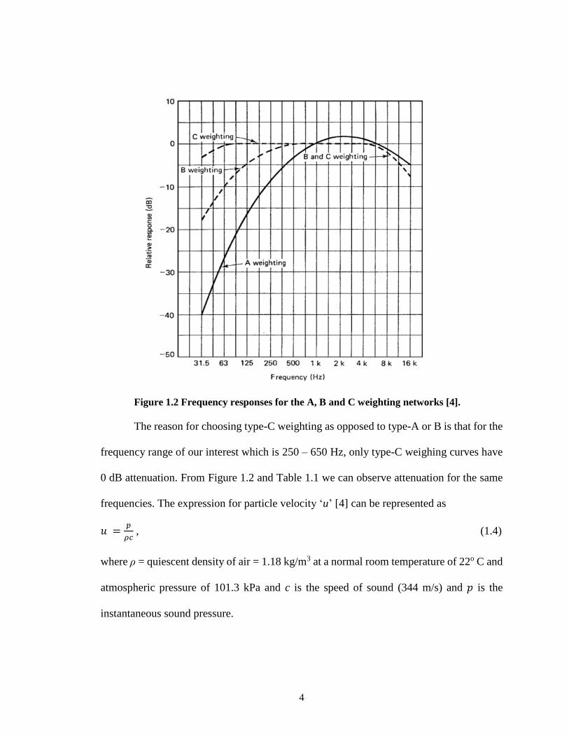
Figure 1.2 Frequency responses for the A, B and C weighting networks [4].

The reason for choosing type-C weighting as opposed to type-A or B is that for the

frequency range of our interest which is 250 – 650 Hz, only type-C weighing curves have

0 dB attenuation. From Figure 1.2 and Table 1.1 we can observe attenuation for the same

frequencies. The expression for particle velocity ‘u’ [4] can be represented as

𝑢 =𝑝

𝜌𝑐 , (1.4)

where ρ = quiescent density of air = 1.18 kg/m3 at a normal room temperature of 22o C and

atmospheric pressure of 101.3 kPa and c is the speed of sound (344 m/s) and 𝑝 is the

instantaneous sound pressure.

5

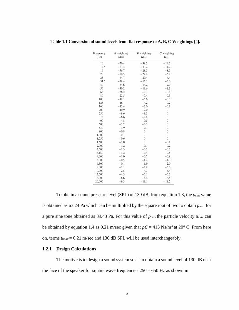
Table 1.1 Conversion of sound levels from flat response to A, B, C Weightings [4].

To obtain a sound pressure level (SPL) of 130 dB, from equation 1.3, the prms value

is obtained as 63.24 Pa which can be multiplied by the square root of two to obtain pmax for

a pure sine tone obtained as 89.43 Pa. For this value of pmax the particle velocity umax can

be obtained by equation 1.4 as 0.21 m/sec given that 𝜌𝐶 = 413 Ns/m3 at 20° C. From here

on, terms umax = 0.21 m/sec and 130 dB SPL will be used interchangeably.

1.2.1 Design Calculations

The motive is to design a sound system so as to obtain a sound level of 130 dB near

the face of the speaker for square wave frequencies 250 – 650 Hz as shown in

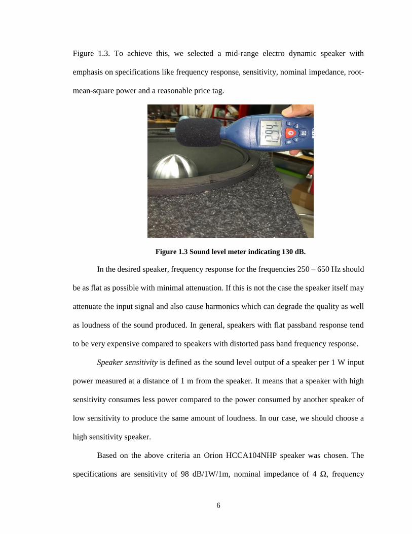
6

Figure 1.3. To achieve this, we selected a mid-range electro dynamic speaker with

emphasis on specifications like frequency response, sensitivity, nominal impedance, root-

mean-square power and a reasonable price tag.

Figure 1.3 Sound level meter indicating 130 dB.

In the desired speaker, frequency response for the frequencies 250 – 650 Hz should

be as flat as possible with minimal attenuation. If this is not the case the speaker itself may

attenuate the input signal and also cause harmonics which can degrade the quality as well

as loudness of the sound produced. In general, speakers with flat passband response tend

to be very expensive compared to speakers with distorted pass band frequency response.

Speaker sensitivity is defined as the sound level output of a speaker per 1 W input

power measured at a distance of 1 m from the speaker. It means that a speaker with high

sensitivity consumes less power compared to the power consumed by another speaker of

low sensitivity to produce the same amount of loudness. In our case, we should choose a

high sensitivity speaker.

Based on the above criteria an Orion HCCA104NHP speaker was chosen. The

specifications are sensitivity of 98 dB/1W/1m, nominal impedance of 4 Ω, frequency

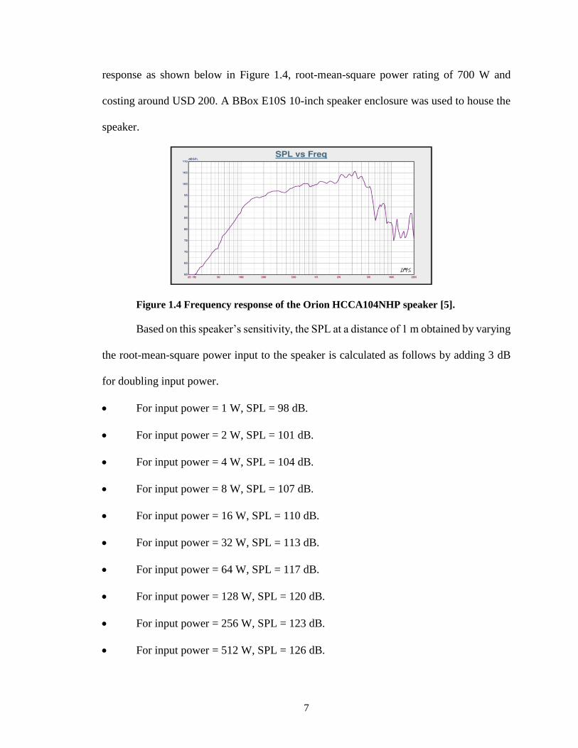
7

response as shown below in Figure 1.4, root-mean-square power rating of 700 W and

costing around USD 200. A BBox E10S 10-inch speaker enclosure was used to house the

speaker.

Figure 1.4 Frequency response of the Orion HCCA104NHP speaker [5].

Based on this speaker’s sensitivity, the SPL at a distance of 1 m obtained by varying

the root-mean-square power input to the speaker is calculated as follows by adding 3 dB

for doubling input power.

• For input power = 1 W, SPL = 98 dB.










8


In our experimental setup we were able to obtain an SPL of 130 dB at a distance of

2.5 cm from the speaker. The speaker was driven by a single channel of an Auna Dark Star

Series 4 channel, 4000 W car amplifier for which a Tektronix AFG1022 function generator

operating in sweep mode with start, stop frequency range selected as 250 Hz and 650 Hz

respectively was used as a signal source. On the function generator, the sweep time period

was set to 500 seconds with square waveform of 300 mV (peak to peak) applied. In both

variant-1 and variant-2 of the experimental setup the sound system remains the same. The

experiments were conducted at the Harris County Mosquito and Vector Control division,

Houston, TX. All the mosquitoes used in the experiments belong to the species Culex

Quinquefasciatus.

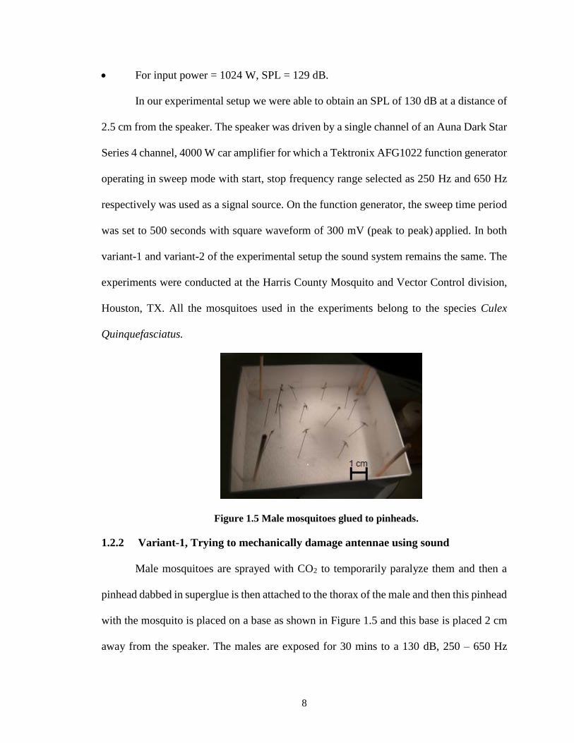
Figure 1.5 Male mosquitoes glued to pinheads.

1.2.2 Variant-1, Trying to mechanically damage antennae using sound

Male mosquitoes are sprayed with CO2 to temporarily paralyze them and then a

pinhead dabbed in superglue is then attached to the thorax of the male and then this pinhead

with the mosquito is placed on a base as shown in Figure 1.5 and this base is placed 2 cm

away from the speaker. The males are exposed for 30 mins to a 130 dB, 250 – 650 Hz

9

square wave frequency sweep sound and are then inspected under a stereo microscope. The

motive of variant-1 is to observe any physiological damage to the male mosquito’s antenna

due to exposure to 130 dB SPL.

1.2.3 Variant-2, Attributing deafening to the number of larvae

Variant-1 does not give us information about loss of hearing sensitivity in the

exposed males. In variant-2, the motive is to see if 30 minutes of exposure to 130 dB SPL

can affect the hearing process of male mosquitoes and potentially incapacitate their ability

to locate and pursue a female to mate. The hypothesis to be tested in variant-2 is “Does

exposure to loud sound reduce the number of larvae.”

We used five mosquito cages wherein the length, width and height of the first two

cages are 90, 75, 75 cm respectively and were called “big cages.” The other three cages

look like a cube with a side length of 30 cm and were called “small cages.”

We used two big cages wherein the first cage was for the control group of

mosquitoes and the other cage was for the exposed group. Each cage housed 35 males and

35 females. These big cages were chosen so as to discourage chance encounters. The

control cage consisted of 35 virgin males and 35 virgin females which were not exposed to

130 dB SPL. The exposed cage consisted of 35 virgin males which were exposed to an

SPL of 130 dB, a 250 – 650 Hz, square wave frequency sweep for 30 minutes and 35 virgin

females which weren’t exposed to sound.

The males and females in both cages belonged to the same batch of larvae, the

males and females were 2 – 3 days old when they were introduced to both the cages. Hence,

the only difference between the control and the exposed cages is that the males in the

control cage were not exposed to sound and the males in the second big cage were exposed

10

to sound before being introduced into the cage. Care was taken to ensure that both the

exposed and unexposed males had the same temperature (30o C) and relative humidity

(80%) around them. Mosquitoes were introduced into both the cages on day one, cups

containing sugar solution with attached cotton wicks were maintained for mosquitoes to

feed from the day mosquitoes were introduced into cages. The cages were left undisturbed

for the next seven days to facilitate mating.

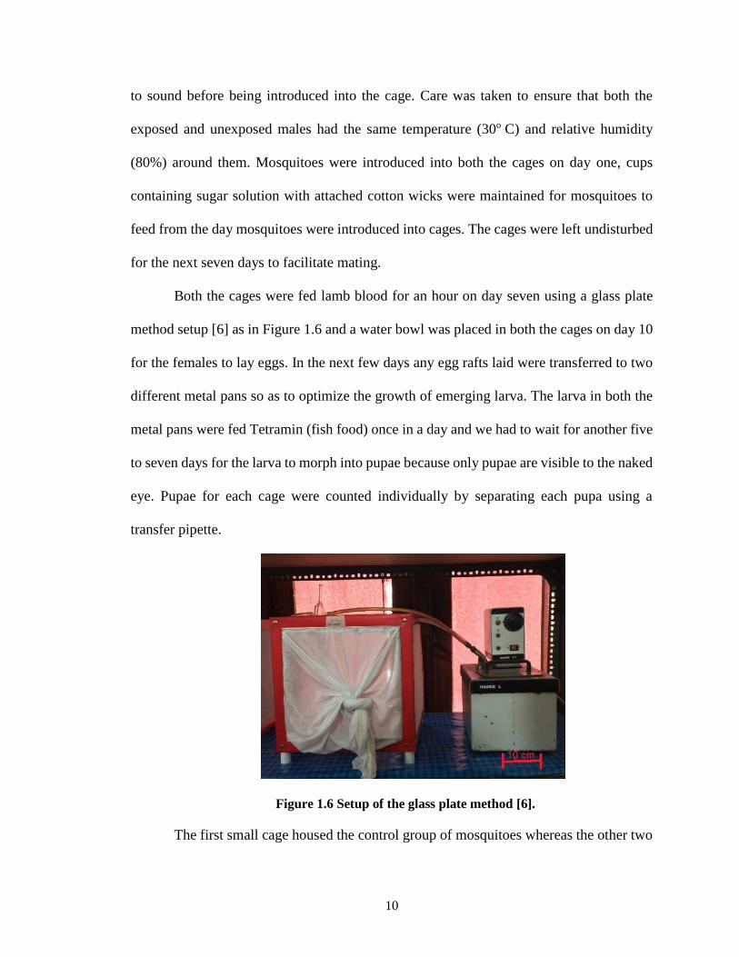
Both the cages were fed lamb blood for an hour on day seven using a glass plate

method setup [6] as in Figure 1.6 and a water bowl was placed in both the cages on day 10

for the females to lay eggs. In the next few days any egg rafts laid were transferred to two

different metal pans so as to optimize the growth of emerging larva. The larva in both the

metal pans were fed Tetramin (fish food) once in a day and we had to wait for another five

to seven days for the larva to morph into pupae because only pupae are visible to the naked

eye. Pupae for each cage were counted individually by separating each pupa using a

transfer pipette.

Figure 1.6 Setup of the glass plate method [6].

The first small cage housed the control group of mosquitoes whereas the other two

11

small cages housed the exposed groups. The control small cage consisted of ten pairs of

virgin males and females both unexposed to 130 dB SPL. The second small cage contained

ten virgin exposed males and ten virgin unexposed females. The third cage consisted of ten

pairs of virgin males and females with all the pairs exposed to 130 dB SPL. The rest of the

procedures remain the same for the big cages and also the small cages.

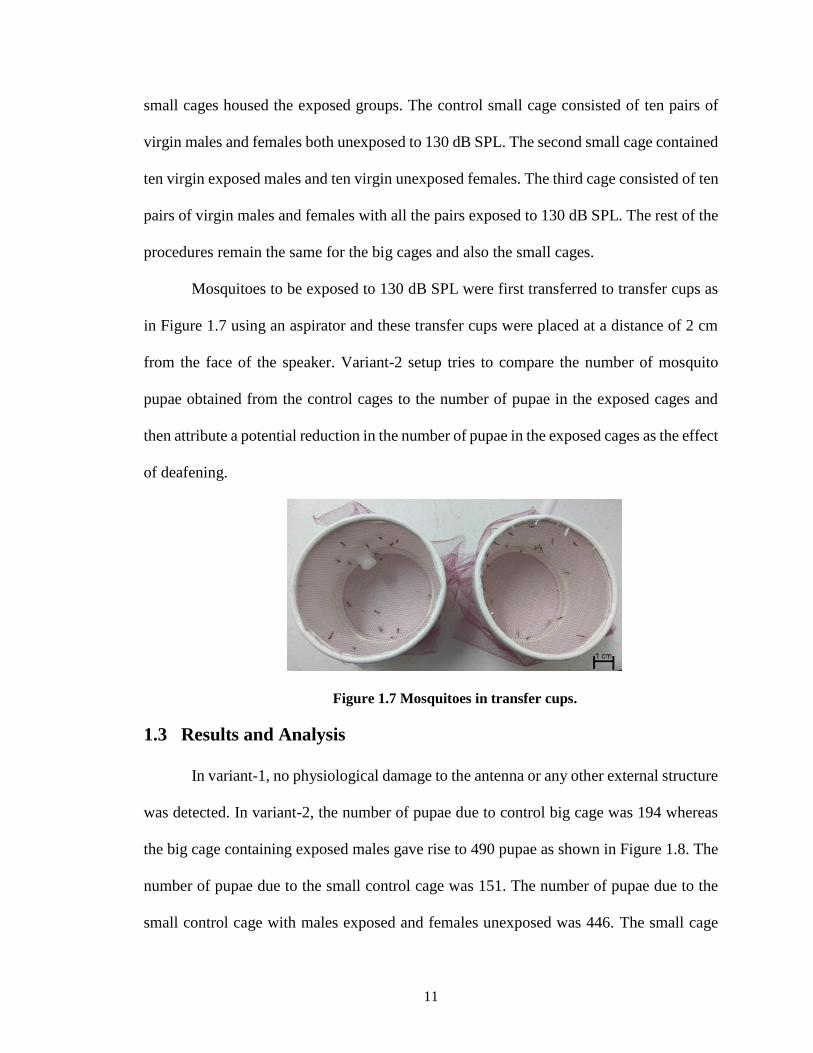
Mosquitoes to be exposed to 130 dB SPL were first transferred to transfer cups as

in Figure 1.7 using an aspirator and these transfer cups were placed at a distance of 2 cm

from the face of the speaker. Variant-2 setup tries to compare the number of mosquito

pupae obtained from the control cages to the number of pupae in the exposed cages and

then attribute a potential reduction in the number of pupae in the exposed cages as the effect

of deafening.

Figure 1.7 Mosquitoes in transfer cups.

1.3 Results and Analysis

In variant-1, no physiological damage to the antenna or any other external structure

was detected. In variant-2, the number of pupae due to control big cage was 194 whereas

the big cage containing exposed males gave rise to 490 pupae as shown in Figure 1.8. The

number of pupae due to the small control cage was 151. The number of pupae due to the

small control cage with males exposed and females unexposed was 446. The small cage

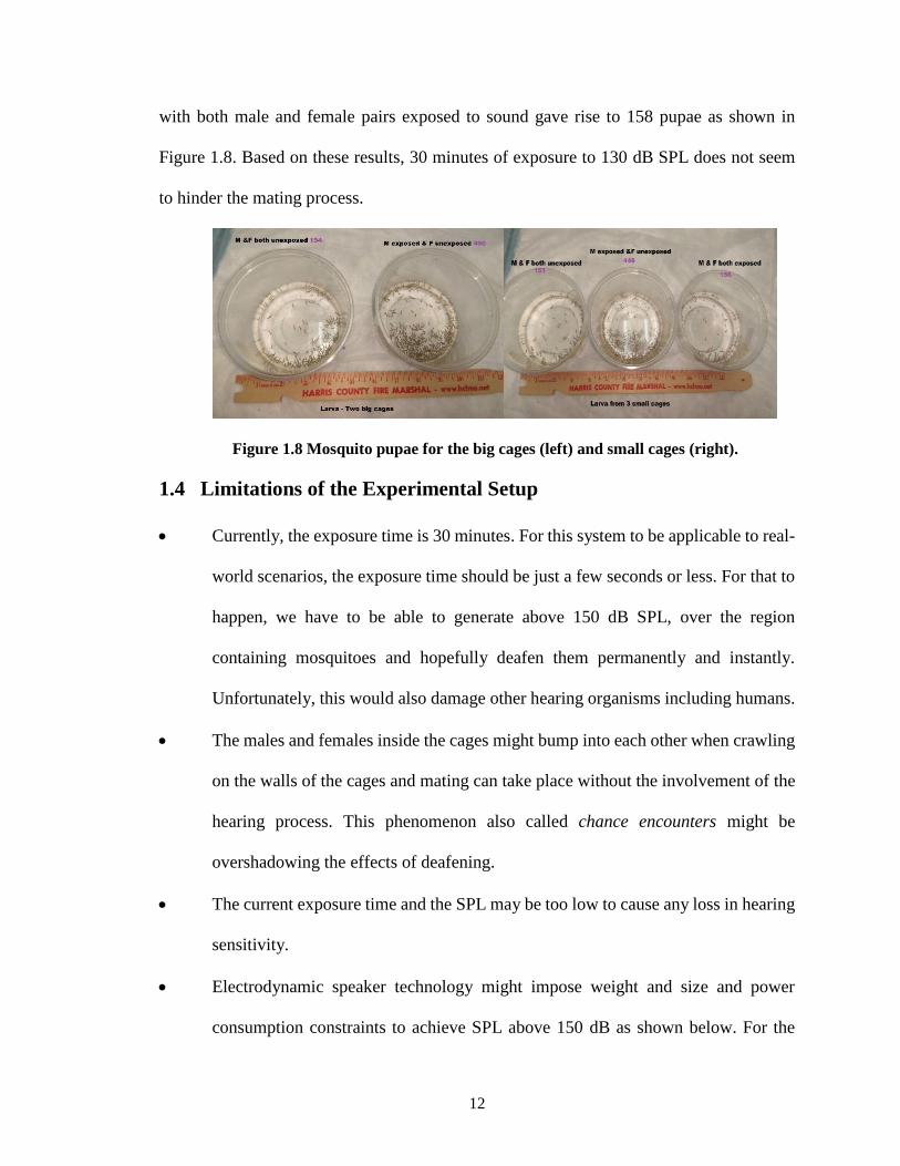
12

with both male and female pairs exposed to sound gave rise to 158 pupae as shown in

Figure 1.8. Based on these results, 30 minutes of exposure to 130 dB SPL does not seem

to hinder the mating process.

Figure 1.8 Mosquito pupae for the big cages (left) and small cages (right).

1.4 Limitations of the Experimental Setup

• Currently, the exposure time is 30 minutes. For this system to be applicable to real-

world scenarios, the exposure time should be just a few seconds or less. For that to

happen, we have to be able to generate above 150 dB SPL, over the region

containing mosquitoes and hopefully deafen them permanently and instantly.

Unfortunately, this would also damage other hearing organisms including humans.

• The males and females inside the cages might bump into each other when crawling

on the walls of the cages and mating can take place without the involvement of the

hearing process. This phenomenon also called chance encounters might be

overshadowing the effects of deafening.

• The current exposure time and the SPL may be too low to cause any loss in hearing

sensitivity.

• Electrodynamic speaker technology might impose weight and size and power

consumption constraints to achieve SPL above 150 dB as shown below. For the

13

calculations below, it is assumed that the sound waves from all the speakers are

correlated and all the speakers have identical specifications.

1 speaker - 130 dB - 512 W (root-mean-square).

2 speakers - 136 dB - 1024 W.

4 speakers - 142 dB - 2048 W.

8 speakers - 148 dB - 4096 W.

16 speakers - 154 dB - 8192 W.

1.5 Future Work

Counting the number of pupae to account the loss of hearing sensitivity in males

may not accurately gauge the hearing loss due to sound exposure. Instead we could insert

electrodes into the antenna of mosquitoes and then measure the sound evoked potential as

in [7].

We could investigate if any physiological damage can be caused by exposing

mosquitoes to high particle velocity sounds with varying frequencies instead of limiting to

250 – 650 Hz range.

To overcome the size and weight limitations imposed by the electrodynamic

speaker technology, we could use ultrasonic transducers to generate audible sound of very

high SPL based on the principle of acoustic heterodyning [8]. This principle leverages the

non-linear behavior of air at very high SPL.

Since ultrasonic transducers are inherently more directional compared to

electrodynamic speakers, generating directed beams of sound targeting aerial mosquito

swarms is feasible with this technology.

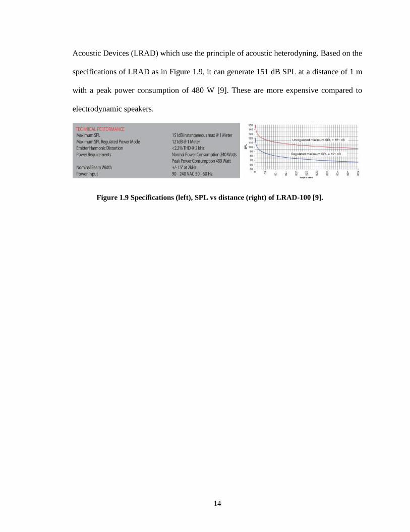
The American Technology Corporation manufactures several Long-Range

14

Acoustic Devices (LRAD) which use the principle of acoustic heterodyning. Based on the

specifications of LRAD as in Figure 1.9, it can generate 151 dB SPL at a distance of 1 m

with a peak power consumption of 480 W [9]. These are more expensive compared to

electrodynamic speakers.

Figure 1.9 Specifications (left), SPL vs distance (right) of LRAD-100 [9].

15

Chapter 2

Underwater Ranging

2.1 Problem Statement

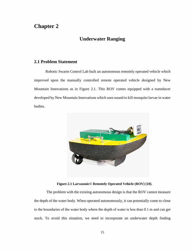
Robotic Swarm Control Lab built an autonomous remotely operated vehicle which

improved upon the manually controlled remote operated vehicle designed by New

Mountain Innovations as in Figure 2.1. This ROV comes equipped with a transducer

developed by New Mountain Innovations which uses sound to kill mosquito larvae in water

bodies.

Figure 2.1 Larvasonic© Remotely Operated Vehicle (ROV) [10].

The problem with the existing autonomous design is that the ROV cannot measure

the depth of the water body. When operated autonomously, it can potentially come to close

to the boundaries of the water body where the depth of water is less than 0.1 m and can get

stuck. To avoid this situation, we need to incorporate an underwater depth finding

16

mechanism. The goal is to design a working depth finding sensor module which solves the

above-mentioned problem.

2.2 Working Principle

An echo sounding technique is used in which an ultrasonic transducer attached to

the ROV, hanging near the surface of the water body, emits sound pulses of 200 KHz

frequency towards the bottom of the water body. These pulses are reflected by the bottom

surface of the water body and then reach the transducer which now acts as a receiver and

develops voltage pulses of 200 KHz frequency whose magnitude is proportional to the

sound intensity level. A detection threshold voltage can be determined for a maximum

depth reading and if the voltage peak of the echo is less than the detection threshold then

it is considered as noise as opposed to the real echo. The time elapsed between pumping a

pulse to the transducer and detecting a threshold voltage is measured [11]. In our

experimental setup the time elapsed is the time duration between the 10th high voltage input

sine wave and the 16th received echo sine wave. The calculated depth ‘d’ in terms of speed

of sound ‘c’ and time elapsed ‘T’ is given as

𝑑 = 𝑐 × (𝑇

2). (2.1)

In Equation 2.2, ‘t’ is the temperature, ‘S’ is the salinity and ‘z’ is the maximum

depth. The expression for speed of sound is given as

𝑐(𝑡, 𝑧, 𝑆) = 1449.2 + 4.6𝑡 − 5.5 × 10−2𝑡2 + 2.9 × 10−4𝑡3 +

(1.34 − 10−2𝑡)(𝑆 − 35) + 1.6 × 10−2𝑧. (2.2)

Equation 2.2 is only valid for the following limits given by

0 ≤ 𝑡 ≤ 35° 𝐶, (2.3)

0 ≤ 𝑆 ≤ 45 practical salinity unit, and (2.4)

17

0 ≤ 𝑧 ≤ 1000 meters. (2.5)

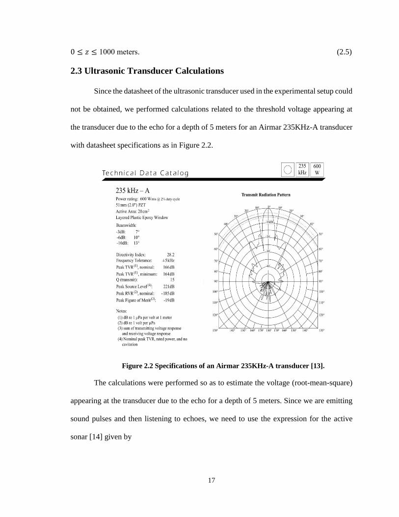
2.3 Ultrasonic Transducer Calculations

Since the datasheet of the ultrasonic transducer used in the experimental setup could

not be obtained, we performed calculations related to the threshold voltage appearing at

the transducer due to the echo for a depth of 5 meters for an Airmar 235KHz-A transducer

with datasheet specifications as in Figure 2.2.

Figure 2.2 Specifications of an Airmar 235KHz-A transducer [13].

The calculations were performed so as to estimate the voltage (root-mean-square)

appearing at the transducer due to the echo for a depth of 5 meters. Since we are emitting

sound pulses and then listening to echoes, we need to use the expression for the active

sonar [14] given by

18

𝐿𝑆

𝑁

= 𝑆𝐿 − 2𝑇𝐿 + 𝑇𝑆 − (𝑁𝐿 − 𝐷𝐼) > 𝐷𝑇. (2.6)

The transmission efficiency (TVR) of an ultrasonic transducer is defined as the

sound pressure produced in the center of the radiated beam at the indicated distance and at

the given excitation voltage whereas the reception efficiency (RVR) of a transducer is the

output open circuit (usually simulated by a 3.9kΩ load) voltage. The transducer directivity,

or radiation pattern (DI), is a sound pressure distribution versus observation angle [15].

From Figure 2.2, the values of TVR, RVR and DI are TVR = 164 dB, RVR = -185 dB, DI =

28.2 dB.

Source level (SL) is always defined in terms of either a fixed voltage input or power

of the transducer. If the input voltage to the transducer is assumed to be 200 V (root-mean

-square), the expression for the sound intensity level or source level [16] at a distance of

1m from the transducer is given as

𝑆𝐿 = 𝑇𝑉𝑅 + 20 log (𝑉𝑖𝑛,

1) dB and (2.7)

𝑆𝐿 = 164 + 20log (200) = 210 dB. (2.8)

Transmission loss (TL) can be attributed to the spherical spreading of sound and

also to the absorption phenomenon of water. TL can be found by adding both these terms

together as in Equation 2.9 below where r is depth in meters and α is the absorption of

sound in seawater. Here α = 90.686 dB/km based on [17], for f = 235 KHz, T = 20° C, r =

5m, S = 35 ppt, pH = 8 from [18]. The expression for TL is given by

𝑇𝐿 = 20 log(𝑟) + [𝛼 × (𝑟 × 10−3)] dB and (2.9)

𝑇𝐿 = 20 log(5) + [90.68 × (5 × 10−3)] 𝑑𝐵 = 14.43 dB. (2.10)

When an active sonar pulse is transmitted into the water, some of the sound reflects

off of the target. The ratio of the intensity of the reflected wave at a distance of one yard

19

to the incident sound wave (in dB) is the target strength (TS) [14].

If only 10% of incident sound is reflected by the bottom surface of the water body,

then TS can be obtained as

𝑇𝑆 = 10 log (𝐼𝑛𝑡𝑒𝑛𝑠𝑖𝑡𝑦 𝑜𝑓 𝑟𝑒𝑓𝑙𝑒𝑐𝑡𝑒𝑑 𝑠𝑜𝑢𝑛𝑑

𝐼𝑛𝑡𝑒𝑛𝑠𝑖𝑡𝑦 𝑜𝑓 𝑖𝑛𝑐𝑖𝑑𝑒𝑛𝑡 𝑠𝑜𝑢𝑛𝑑) = −10 dB. (2.11)

The noise level (NL) in a water body is highly variable, the average value is

assumed to be 30 dB, hence NL = 30 dB.

By substituting the calculated values from Equations 2.8, 2.10 and 2.11 into

Equation 2.6, we get the signal to noise ratio ( 𝐿𝑆

𝑁

) as

𝐿𝑆

𝑁

= 210 − [2 × (14.43)] + (−10) − 30 + 28.2 𝑑𝐵 = 169.36 dB. (2.12)

The voltage appearing across the terminals of the transducer when receiving an

echo can be obtained by computing 𝑉𝑖𝑛 𝑑𝐵 as

𝑉𝑖𝑛 𝑑𝐵 = 𝐿𝑆

𝑁

+ 𝑅𝑉𝑅 = 169.36 + (−185) 𝑑𝐵 = −15.64 dB. (2.13)

The root-mean-square value of the voltage due to echo can obtained from the

Equation 2.14. The voltage corresponding to the echo received due to the application of a

200 KHz, 200 V(root-mean-square) input to the Airmar 235K-A transducer is given by

𝑉𝑖𝑛 𝑑𝐵 = 20 log (𝑉𝑒𝑐ℎ𝑜

1) = −15.64 dB and (2.14)

𝑉𝑒𝑐ℎ𝑜 = 0.165 V . (2.15)

Any 𝑉𝑒𝑐ℎ𝑜 less than 0.165 V will be treated as noise. Only if 𝑉𝑒𝑐ℎ𝑜 is greater than

0.165 V can the voltage signal be distinguished from noise.

20

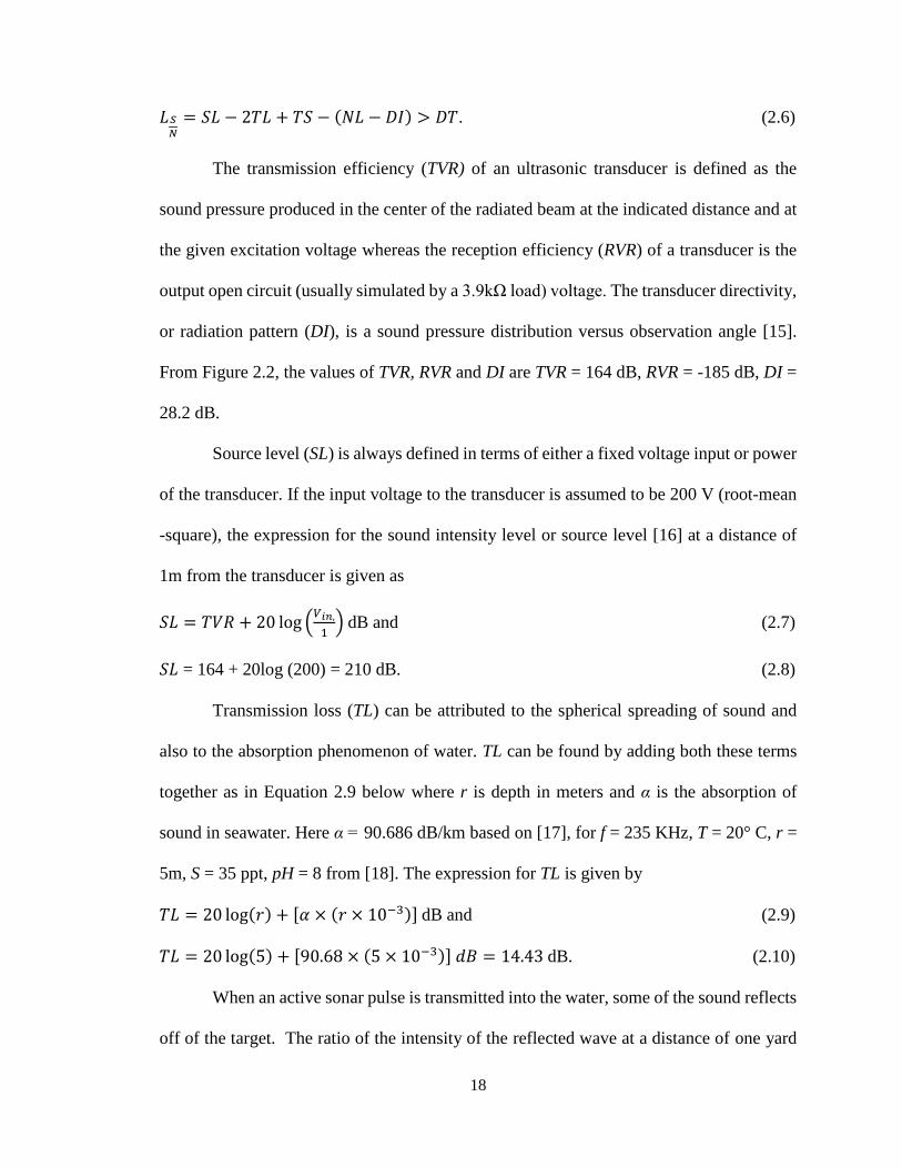
2.4 Analog Circuit Design

Initially, the goal was to separate an ultrasonic transducer from a wireless portable

fish finder and build the analog circuit in conjunction with a microcontroller, to drive the

transducer and use the same transducer to receive the echoes and thereby compute depth.

The analog circuit was designed on Multisim Live and the waveforms of each stage with

respective color codes are represented in Figure 2.3.

Figure 2.3 Circuit diagram and simulation of the driver and feedback circuit.

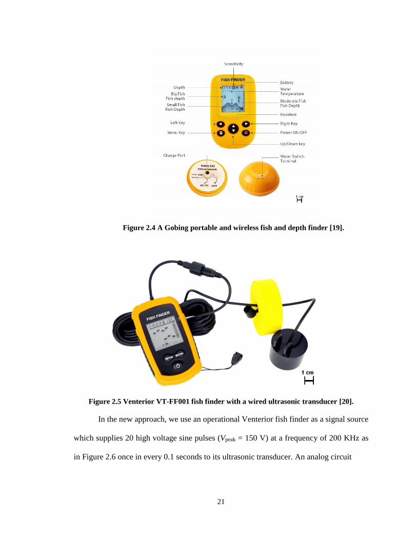
The goal was to eliminate all the components inside the Gobing wireless fish finder

shown in Figure 2.4 and use the ultrasonic transducer alone, driven by the analog circuit

shown in Figure 2.3. The Wein bridge oscillator, amplifier, emitter follower and the

feedback circuit were tested individually. Due to the time constraint, this approach was

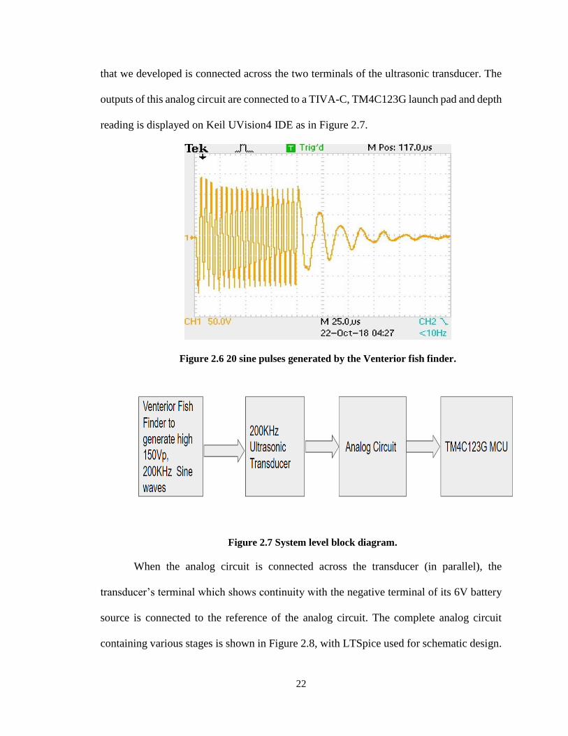
abandoned and a Venterior VT-FF001 portable fish finder with a wired ultrasonic

transducer as in Figure 2.5 was used.

21

Figure 2.4 A Gobing portable and wireless fish and depth finder [19].

Figure 2.5 Venterior VT-FF001 fish finder with a wired ultrasonic transducer [20].

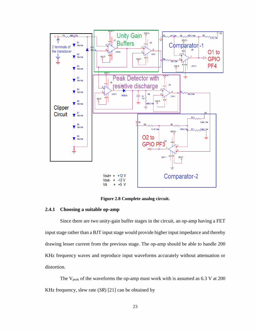
In the new approach, we use an operational Venterior fish finder as a signal source

which supplies 20 high voltage sine pulses (Vpeak = 150 V) at a frequency of 200 KHz as

in Figure 2.6 once in every 0.1 seconds to its ultrasonic transducer. An analog circuit

22

that we developed is connected across the two terminals of the ultrasonic transducer. The

outputs of this analog circuit are connected to a TIVA-C, TM4C123G launch pad and depth

reading is displayed on Keil UVision4 IDE as in Figure 2.7.

Figure 2.6 20 sine pulses generated by the Venterior fish finder.

Figure 2.7 System level block diagram.

When the analog circuit is connected across the transducer (in parallel), the

transducer’s terminal which shows continuity with the negative terminal of its 6V battery

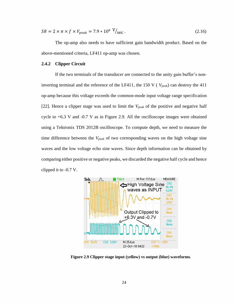
source is connected to the reference of the analog circuit. The complete analog circuit

containing various stages is shown in Figure 2.8, with LTSpice used for schematic design.

23

Figure 2.8 Complete analog circuit.

2.4.1 Choosing a suitable op-amp

Since there are two unity-gain buffer stages in the circuit, an op-amp having a FET

input stage rather than a BJT input stage would provide higher input impedance and thereby

drawing lesser current from the previous stage. The op-amp should be able to handle 200

KHz frequency waves and reproduce input waveforms accurately without attenuation or

distortion.

The Vpeak of the waveforms the op-amp must work with is assumed as 6.3 V at 200

KHz frequency, slew rate (SR) [21] can be obtained by

24

𝑆𝑅 = 2 × 𝜋 × 𝑓 × 𝑉𝑝𝑒𝑎𝑘 = 7.9 ∗ 106 V sec⁄ . (2.16)

The op-amp also needs to have sufficient gain bandwidth product. Based on the

above-mentioned criteria, LF411 op-amp was chosen.

2.4.2 Clipper Circuit

If the two terminals of the transducer are connected to the unity gain buffer’s non-

inverting terminal and the reference of the LF411, the 150 V ( Vpeak) can destroy the 411

op-amp because this voltage exceeds the common-mode input voltage range specification

[22]. Hence a clipper stage was used to limit the Vpeak of the positive and negative half

cycle to +6.3 V and -0.7 V as in Figure 2.9. All the oscilloscope images were obtained

using a Tektronix TDS 2012B oscilloscope. To compute depth, we need to measure the

time difference between the Vpeak of two corresponding waves on the high voltage sine

waves and the low voltage echo sine waves. Since depth information can be obtained by

comparing either positive or negative peaks, we discarded the negative half cycle and hence

clipped it to -0.7 V.

Figure 2.9 Clipper stage input (yellow) vs output (blue) waveforms.

25

The reason for choosing nine diodes in series for handling the positive half cycle is

to allow a sufficient voltage window for echoes. The Vpeak of the echoes in our experimental

setup for the shortest distance between the transducer and the bottom of the 75-gallon

container was found to be less than 4 V and hence during the positive half cycle, echoes

are unattenuated. 1N4148 small signal diodes were used because of their low reverse

recovery time of around 4 ns [23].

Zener diodes were not used instead of diodes because there is a possibility of

loading the driver circuit so that the Zener diode acts like a voltage regulator. A 500 mW

resistor was chosen so that the power dissipation is well below 500 mW.

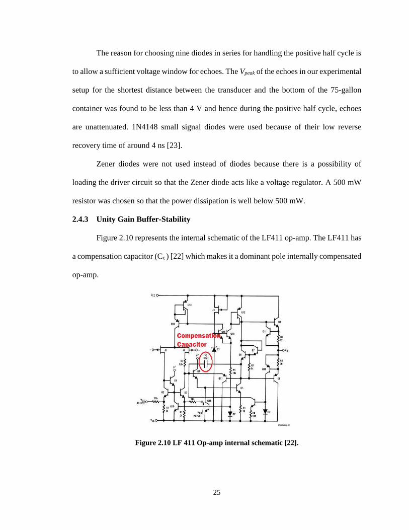
2.4.3 Unity Gain Buffer-Stability

Figure 2.10 represents the internal schematic of the LF411 op-amp. The LF411 has

a compensation capacitor (Cc ) [22] which makes it a dominant pole internally compensated

op-amp.

Figure 2.10 LF 411 Op-amp internal schematic [22].

26

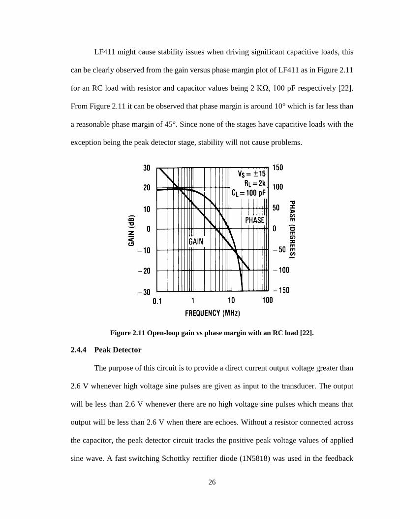
LF411 might cause stability issues when driving significant capacitive loads, this

can be clearly observed from the gain versus phase margin plot of LF411 as in Figure 2.11

for an RC load with resistor and capacitor values being 2 KΩ, 100 pF respectively [22].

From Figure 2.11 it can be observed that phase margin is around 10° which is far less than

a reasonable phase margin of 45°. Since none of the stages have capacitive loads with the

exception being the peak detector stage, stability will not cause problems.

Figure 2.11 Open-loop gain vs phase margin with an RC load [22].

2.4.4 Peak Detector

The purpose of this circuit is to provide a direct current output voltage greater than

2.6 V whenever high voltage sine pulses are given as input to the transducer. The output

will be less than 2.6 V whenever there are no high voltage sine pulses which means that

output will be less than 2.6 V when there are echoes. Without a resistor connected across

the capacitor, the peak detector circuit tracks the positive peak voltage values of applied

sine wave. A fast switching Schottky rectifier diode (1N5818) was used in the feedback

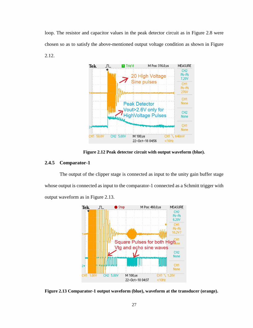
27

loop. The resistor and capacitor values in the peak detector circuit as in Figure 2.8 were

chosen so as to satisfy the above-mentioned output voltage condition as shown in Figure

2.12.

Figure 2.12 Peak detector circuit with output waveform (blue).

2.4.5 Comparator-1

The output of the clipper stage is connected as input to the unity gain buffer stage

whose output is connected as input to the comparator-1 connected as a Schmitt trigger with

output waveform as in Figure 2.13.

Figure 2.13 Comparator-1 output waveform (blue), waveform at the transducer (orange).

28

LM111 was chosen as a comparator because its response time is around 0.2 µs [24]

which is significantly small compared to the time period of the 200 KHz sine wave (5 µs).

The resistor values are calculated based on [25] to obtain threshold values as +0.1 V and

-0.1 V. Since the input terminal is the inverting terminal, if the input voltage is greater than

0.1 V, output goes to zero volts and if the input voltage is less than -0.1 V, output goes to

+5 V.

The purpose of this comparator is to convert the high voltage sine waves and low

voltage echo sine waves into square pulses which are then fed to an edge-triggered digital

pin PF4 on the TM4C123G microcontroller.

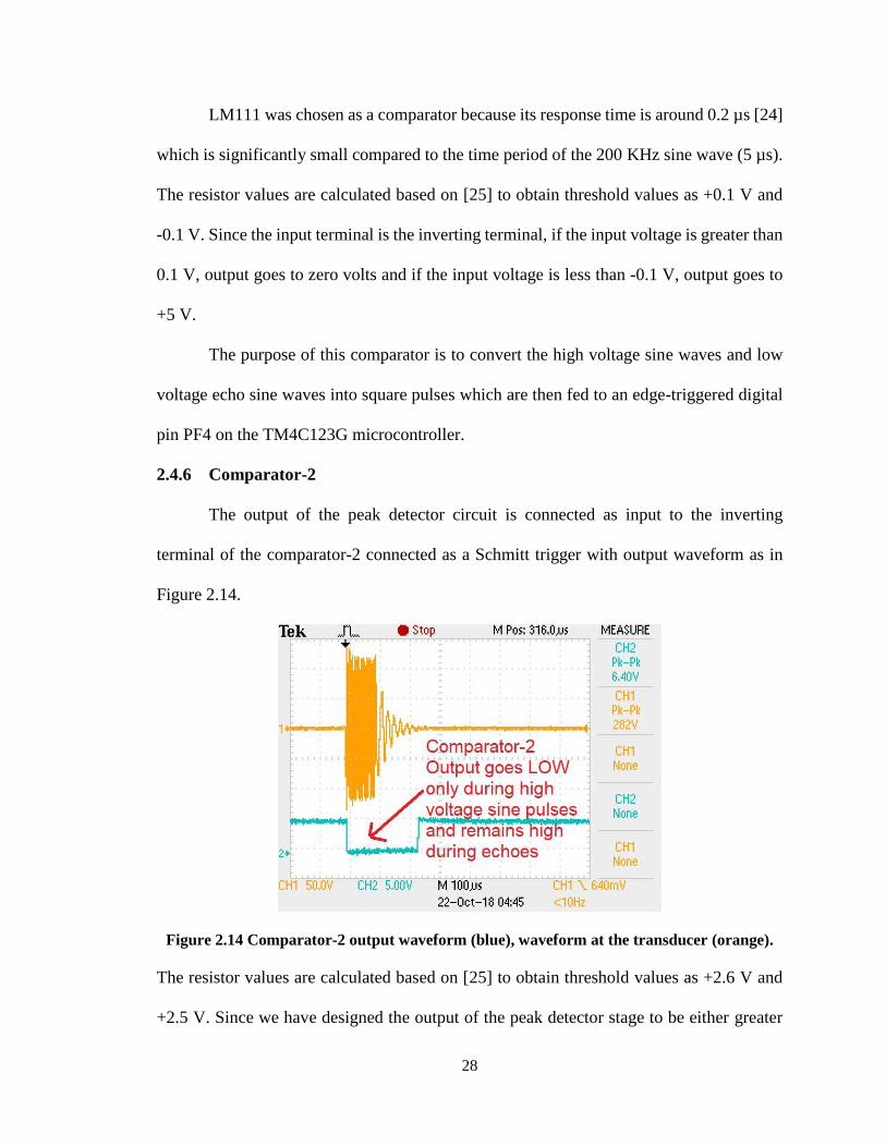
2.4.6 Comparator-2

The output of the peak detector circuit is connected as input to the inverting

terminal of the comparator-2 connected as a Schmitt trigger with output waveform as in

Figure 2.14.

Figure 2.14 Comparator-2 output waveform (blue), waveform at the transducer (orange).

The resistor values are calculated based on [25] to obtain threshold values as +2.6 V and

+2.5 V. Since we have designed the output of the peak detector stage to be either greater

29

than 2.6 V or less than 2.6 V, this means that during the application of high voltage pulses

to the transducer, the output goes to zero volts and the output will change to +5 V state and

will remain at that voltage till the next set of high voltage pulses are applied across the

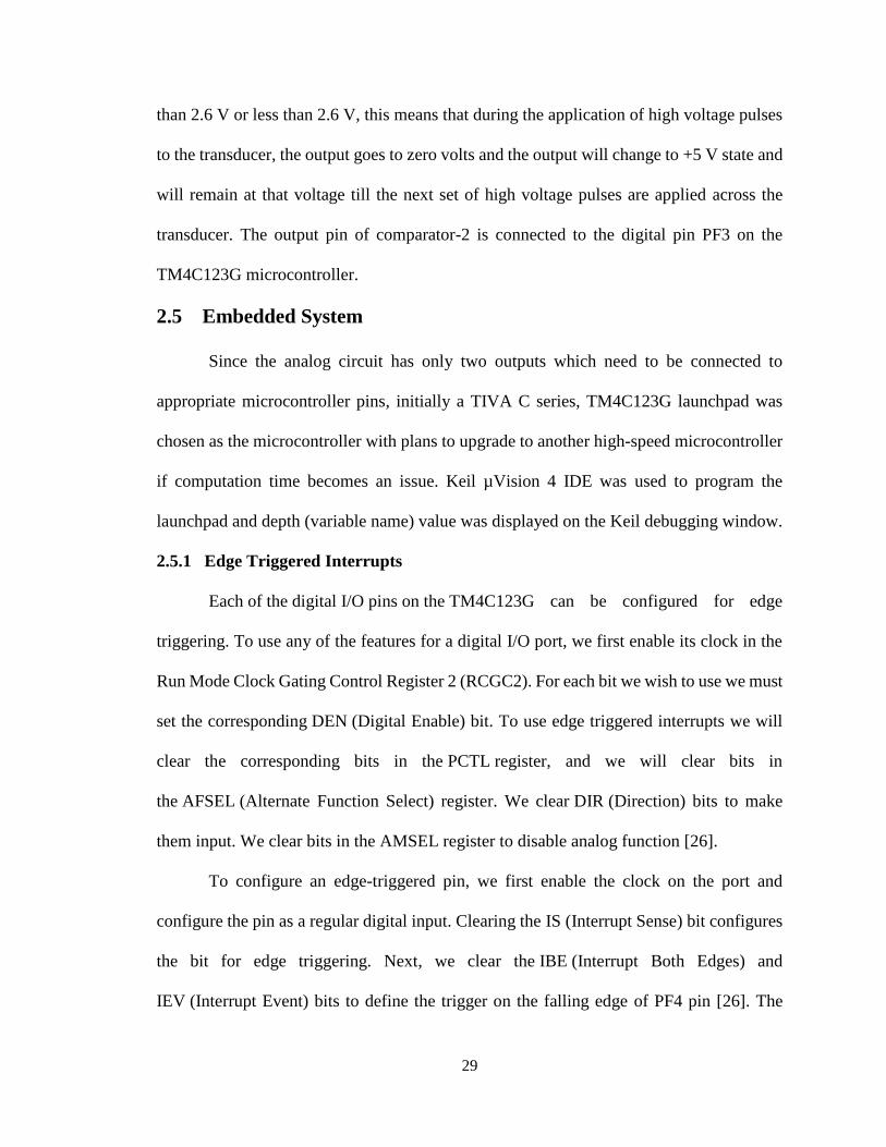
transducer. The output pin of comparator-2 is connected to the digital pin PF3 on the

TM4C123G microcontroller.

2.5 Embedded System

Since the analog circuit has only two outputs which need to be connected to

appropriate microcontroller pins, initially a TIVA C series, TM4C123G launchpad was

chosen as the microcontroller with plans to upgrade to another high-speed microcontroller

if computation time becomes an issue. Keil µVision 4 IDE was used to program the

launchpad and depth (variable name) value was displayed on the Keil debugging window.

2.5.1 Edge Triggered Interrupts

Each of the digital I/O pins on the TM4C123G can be configured for edge

triggering. To use any of the features for a digital I/O port, we first enable its clock in the

Run Mode Clock Gating Control Register 2 (RCGC2). For each bit we wish to use we must

set the corresponding DEN (Digital Enable) bit. To use edge triggered interrupts we will

clear the corresponding bits in the PCTL register, and we will clear bits in

the AFSEL (Alternate Function Select) register. We clear DIR (Direction) bits to make

them input. We clear bits in the AMSEL register to disable analog function [26].

To configure an edge-triggered pin, we first enable the clock on the port and

configure the pin as a regular digital input. Clearing the IS (Interrupt Sense) bit configures

the bit for edge triggering. Next, we clear the IBE (Interrupt Both Edges) and

IEV (Interrupt Event) bits to define the trigger on the falling edge of PF4 pin [26]. The

30

conditions that need to be true for an edge triggered interrupt to be requested are given

below and these have to be met simultaneously [26]:

• The trigger flag bit is set (RIS).

• The arm bit is set (IME).

• The level of the edge-triggered interrupt must be less than BASEPRI.

• The edge-triggered interrupt must be enabled in the NVIC_EN0_R.

• The I bit, the bit zero of the special register PRIMASK, is zero.

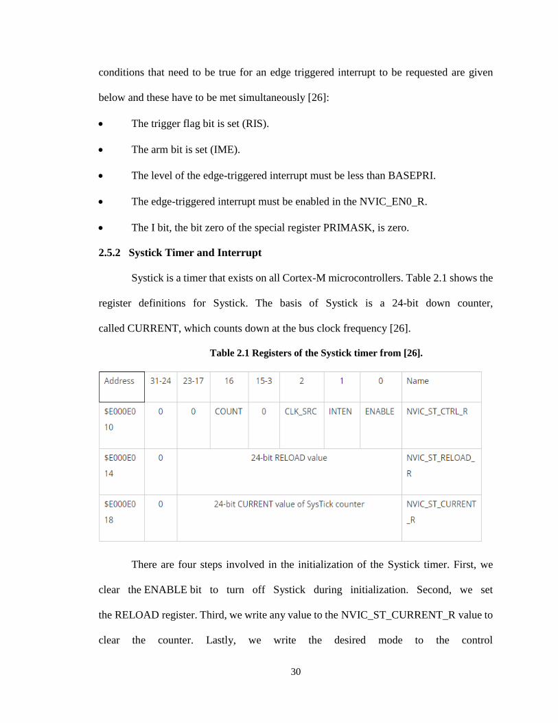
2.5.2 Systick Timer and Interrupt

Systick is a timer that exists on all Cortex-M microcontrollers. Table 2.1 shows the

register definitions for Systick. The basis of Systick is a 24-bit down counter,

called CURRENT, which counts down at the bus clock frequency [26].

Table 2.1 Registers of the Systick timer from [26].

There are four steps involved in the initialization of the Systick timer. First, we

clear the ENABLE bit to turn off Systick during initialization. Second, we set

the RELOAD register. Third, we write any value to the NVIC_ST_CURRENT_R value to

clear the counter. Lastly, we write the desired mode to the control

31

register, NVIC_ST_CTRL_R. The mode involves the CLK_SRC INTEN and ENABLE

bits. We will set CLK_SRC=1, so the counter runs off the system clock. We will also

set INTEN bit so that Systick interrupts are enabled. We need to set the ENABLE bit so

the counter will run. Once the initialization is complete, the timer starts to count down,

i.e., CURRENT is decremented once every bus cycle [26]. Since we are using PLL to

increase the clock frequency to 80 MHz so as to reduce the computation time of each

instruction, the Systick counter decrements every 12.5 ns.

When the CURRENT value counts down from 1 to 0, the COUNT flag is set. On

the next clock, the CURRENT is loaded with the RELOAD value. In this way, the Systick

counter is continuously decrementing. Since the RELOAD value is set to 0x00FFFFFF, so

the CURRENT value is a simple indicator of what count is now. Noting what the count

was at some point and then what it is now, allows us to calculate the time that has elapsed

[26]. The Systick timer with the current 80 MHz clock source setting can measure a

maximum time difference of nearly 0.2 s. This is not a limitation in our experimental setup

because the time corresponding to the maximum depth of 10m is, far less than 0.2 s.

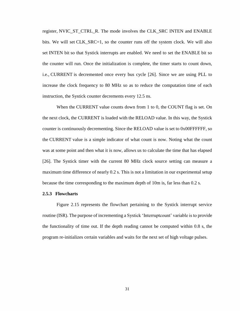
2.5.3 Flowcharts

Figure 2.15 represents the flowchart pertaining to the Systick interrupt service

routine (ISR). The purpose of incrementing a Systick ‘Interruptcount’ variable is to provide

the functionality of time out. If the depth reading cannot be computed within 0.8 s, the

program re-initializes certain variables and waits for the next set of high voltage pulses.

32

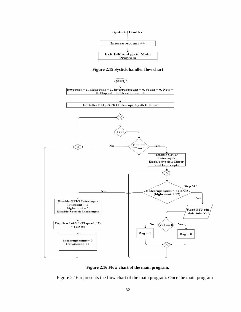
Figure 2.15 Systick handler flow chart

Figure 2.16 Flow chart of the main program.

Figure 2.16 represents the flow chart of the main program. Once the main program

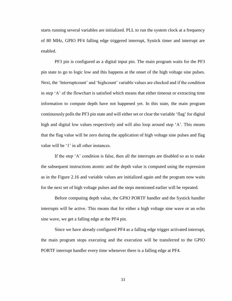
33

starts running several variables are initialized. PLL to run the system clock at a frequency

of 80 MHz, GPIO PF4 falling edge triggered interrupt, Systick timer and interrupt are

enabled.

PF3 pin is configured as a digital input pin. The main program waits for the PF3

pin state to go to logic low and this happens at the onset of the high voltage sine pulses.

Next, the ‘Interruptcount’ and ‘highcount’ variable values are checked and if the condition

in step ‘A’ of the flowchart is satisfied which means that either timeout or extracting time

information to compute depth have not happened yet. In this state, the main program

continuously polls the PF3 pin state and will either set or clear the variable ‘flag’ for digital

high and digital low values respectively and will also loop around step ‘A’. This means

that the flag value will be zero during the application of high voltage sine pulses and flag

value will be ‘1’ in all other instances.

If the step ‘A’ condition is false, then all the interrupts are disabled so as to make

the subsequent instructions atomic and the depth value is computed using the expression

as in the Figure 2.16 and variable values are initialized again and the program now waits

for the next set of high voltage pulses and the steps mentioned earlier will be repeated.

Before computing depth value, the GPIO PORTF handler and the Systick handler

interrupts will be active. This means that for either a high voltage sine wave or an echo

sine wave, we get a falling edge at the PF4 pin.

Since we have already configured PF4 as a falling edge trigger activated interrupt,

the main program stops executing and the execution will be transferred to the GPIO

PORTF interrupt handler every time whenever there is a falling edge at PF4.

34

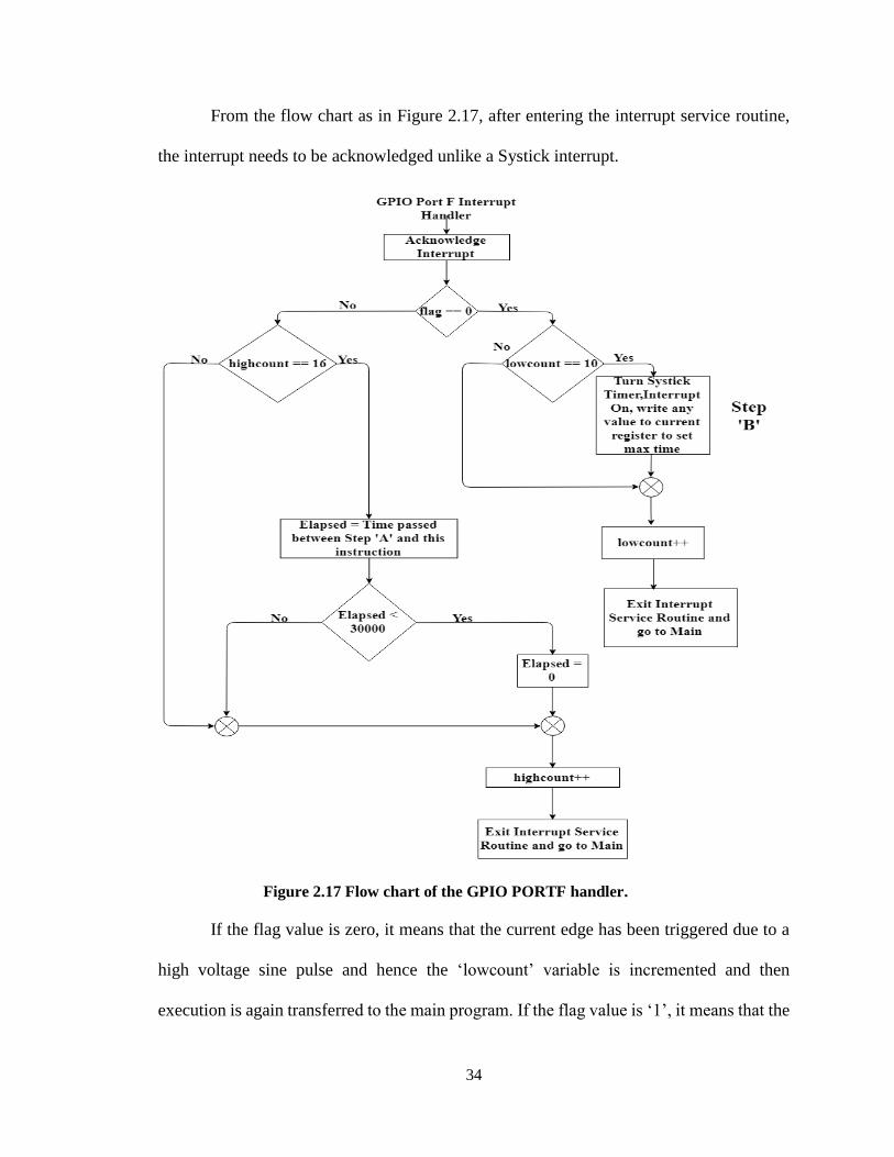
From the flow chart as in Figure 2.17, after entering the interrupt service routine,

the interrupt needs to be acknowledged unlike a Systick interrupt.

Figure 2.17 Flow chart of the GPIO PORTF handler.

If the flag value is zero, it means that the current edge has been triggered due to a

high voltage sine pulse and hence the ‘lowcount’ variable is incremented and then

execution is again transferred to the main program. If the flag value is ‘1’, it means that the

35

current edge has been triggered due to an echo and hence the variable ‘highcount’ will be

incremented. If the ‘lowcount’ value reaches 10, a value will be written to the

NVIC_ST_CURRENT_R to start the timer as in step ’B’ of Figure 2.17 and the ‘lowcount’

value is incremented and execution is again transferred to the main program.

During the execution of PORTF handler, when the flag value is ‘1’ and if the value

of ‘highcount’ is 16, the time elapsed between step ‘B’ and the current step contains the

depth information. If the elapsed value is less than 30000, it has been observed empirically

that the echoes are merging with the high voltage sine pulses due to the close proximity of

the transducer with the floor of the 75-gallon container and hence depth reading for any

value less than 0.28 m will be displayed as zero to avoid errors. The reason for choosing

the time difference between the 10th high voltage pulse and the 16th echo pulse as opposed

to the time difference between the 10th high voltage pulse and the 10th echo pulse can be

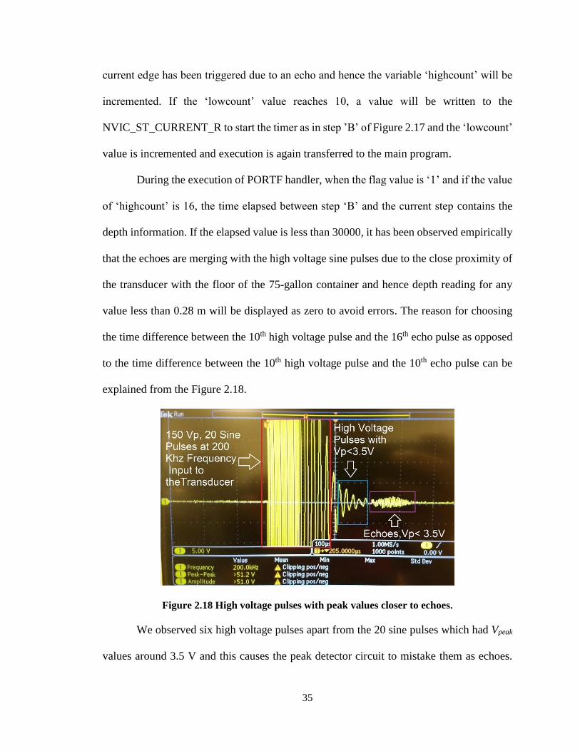
explained from the Figure 2.18.

Figure 2.18 High voltage pulses with peak values closer to echoes.

We observed six high voltage pulses apart from the 20 sine pulses which had Vpeak

values around 3.5 V and this causes the peak detector circuit to mistake them as echoes.

36

Hence ‘highcount’ value for computing the depth was chosen as 16 as opposed to 10.

Furthermore, the frequency of these six sine waves is different from that of the frequency

of the 20 high voltage sine pulses or the echoes.

2.6 Results

The experimental setup was used to determine the depth of a 75-gallon container

having a water level at 0.96 m. Temperature of the water was measured using a Taylor

digital thermometer as 23°C and speed of sound in the tank was calculated from Equation

2.2 as 1495 m/sec. Depth values between 0.28 m and 0.96 m could be accurately obtained

with the experimental setup. A working demonstration can be found at

https://youtu.be/o4eq6Y9oSfk

2.7 Future Work

• Design a circuit to generate high voltage sine pulses at 200 KHz frequency.

• Test the experimental setup in different water bodies.

• Incorporate temperature and salinity sensors.

• Investigate the need of an amplifier stage so as to amplify echoes for greater depths.

• Use a higher frequency transducer to reduce the minimum depth measurement

limitation.

37

Chapter 3

Conclusion

This thesis examined the two hypotheses and learned that exposing mosquitoes to

130 dB of sound for 30 minutes with 250 – 650 Hz square wave frequency sweep does not

seem to cause any physiological damage to the antenna and also does not seem to hinder

the mosquito mating process. Future work should quantify chance encounters, investigate

acoustic heterodyning, measure sound evoked potential after exposure and change

frequencies to observe any other physiological damage apart from hearing.

This thesis also examined the design of an underwater depth finding sensor

module and the experimental setup was able to compute and display the distance between

ultrasonic transducer and the bottom of the 75-gallon container successfully. The minimum

depth range for the experimental setup is found to be 0.28 m. Future work should include

field trials, choosing a higher frequency ultrasonic transducer, developing high voltage sine

wave generating circuitry, incorporating temperature and salinity sensors and also

investigating the need for amplifying echoes.

38

References

[1] Clements, A. N. (1963). The physiology of mosquitoes. New York: Macmillan.

[2] Hoy R. “A boost for hearing in mosquitoes,” Proceedings of the National Academy

of Sciences of the United States of America. 2006;103(45):16619-16620.

doi:10.1073/pnas.0608105103.

[3] Roth, Louis M. "A study of mosquito behavior. An experimental laboratory study

of the sexual behavior of Aedes aegypti (Linnaeus)," The American Midland

Naturalist 40.2 (1948): 265-352.

[4] Raichel, Daniel R. The Science and Applications of Acoustics. Springer, 2011.

[5] Orion HCCA104NHP High Efficiency Mid-range Speaker. (n.d.). Retrieved from

https://www.carid.com/images/orion/speakers/pdf/hcca-nhp-midrange-high-

efficiency-speaker-guide.pdf.

[6] Gunathilaka N, Ranathunge T, Udayanga L, Abeyewickreme W. “Efficacy of blood

sources and artificial blood feeding methods in rearing of Aedes Aegypti (Diptera:

Culicidae) for sterile insect technique and incompatible insect technique

approaches in Sri Lanka,” Biomed Res Int. 2017;2017:3196924.

[7] Christie KW, Sivan-Loukianova E, Smith WC. “Physiological, anatomical, and

behavioral changes after acoustic trauma in Drosophila melanogaster,”

Proceedings of the National Academy of Sciences of the United States of America.

2013;110(38):15449-15454. doi:10.1073/pnas.1307294110.

[8] Norris, E. (1996). U.S. Patent No. US5889870A. Washington, DC: U.S. Patent and

39

Trademark Office.

[9] LRAD 1000 Product Sheet. (n.d.). Retrieved from http://www.oregonstatehospital.

net/d/otherfiles/LRADMilitarySoundWeapon/Product-Sheet-LRAD-

1000_decrypted.pdf.

[10] Larvasonic© remotely operated vehicle (ROV) [Digital image]. (n.d.). Retrieved

from http://www.newmountain.com/product/larvasonic-remotely-operated-

vehicle-rov/.

[11] Borujeni, S. (n.d.). “Ultrasonic underwater depth measurement,” Proceedings of

the 2002 Interntional Symposium on Underwater Technology (Cat. No.02EX556).

doi:10.1109/ut.2002.1002376.

[12] Medwin, H. (1975). “Speed of sound in water: A simple equation for realistic

parameters,” The Journal of the Acoustical Society of America, 58(6), 1318-1319.

doi:10.1121/1.380790.

[13] Technical data catalog, 235 KHz - A, ultrasonic transducer. (n.d.). Retrieved from

http://www.airmar.com/uploads/techdata/235a.pdf.

[14] Urick, R. J. (1983). Principles of Underwater Sound. S.l.: Peninsula Publishing.

[15] L, S., & G, M. (2007). Data acquisition system for air-coupled navigation study ...

Retrieved from http://citeseerx.ist.psu.edu/viewdoc/download?doi=10.1.1.535

.3049&rep= rep1&type=pdf.

[16] Linear and Nonlinear Acoustics. (n.d.). Retrieved from https://www.benthowave.c

om/resources/default.html.

[17] Ainslie, M. A., & Mccolm, J. G. (1998). “A simplified formula for viscous and

chemical absorption in sea water,” The Journal of the Acoustical Society of

40

America, 103(3), 1671-1672. doi:10.1121/1.421258.

[18] Calculation of absorption of sound in seawater. (n.d.). Retrieved from

http://resource.npl.co.uk/acoustics/techguides/seaabsorption/.

[19] Gobing wireless sonar sensor fish finder. (n.d.). Retrieved from

https://www.amazon.com/Gobing-Humminbird-Transducer-Temperature-

Fishfinder/dp/B071JF4VL4.

[20] Venterior VT-FF001 portable fish Finder, fishfinder with wired sonar sensor

transducer. (n.d.). Retrieved from https://www.amazon.com/Venterior-VT-FF001-

Portable-Fishfinder-Transducer/dp/B013DZJDWE.

[21] Choudary, R. D., & Shail, J. B. (n.d.). Linear Integrated Circuits (4th ed.). New Age

Intl Uk.

[22] LF411 datasheet by National Semiconductor. (n.d.). Retrieved from

http://pdf.datasheetcatalog.com/datasheet/nationalsemiconductor/DS005655.PDF.

[23] 1N4148 datasheet by Diodes Incorporated. (n.d.). Retrieved from

http://pdf.datasheetcatalog.com/datasheet/diodes/ds12019.pdf.

[24] LM111 datasheet by National Semiconductors. (n.d.). Retrieved from

http://pdf.datasheetcatalog.com/datasheet/nationalsemiconductor/DS005704.PDF.

[25] Hayes, T. C., & Horowitz, P. (2017). Learning the art of electronics A hands-on lab

course.

[26] Valvano, J. W. (2016). Real-time interfacing to ARM Cortex-M microcontrollers.

USA: Jonathan W. Valvano.

Documents

Deafening Mosquitoes and Underwater Ranging