Embed Size (px)
Citation preview

arX
iv:0
901.
0197
v5 [
mat
h.R
T]
24
Oct
201
0
DECOMPOSITION OF TENSOR PRODUCTS OF MODULAR
IRREDUCIBLE REPRESENTATIONS FOR SL3
(WITH AN APPENDIX BY C.M. RINGEL)
C. BOWMAN, S.R. DOTY, AND S. MARTIN
Abstract. We give an algorithm for working out the indecomposable direct summands ina Krull–Schmidt decomposition of a tensor product of two simple modules for G = SL3 incharacteristics 2 and 3. It is shown that there is a finite family of modules such that everysuch indecomposable summand is expressible as a twisted tensor product of members ofthat family.
Along the way we obtain the submodule structure of various Weyl and tilting modules.Some of the tilting modules that turn up in characteristic 3 are not rigid; these seem toprovide the first example of non-rigid tilting modules for algebraic groups. These non-rigid tilting modules lead to examples of non-rigid projective indecomposable modules forSchur algebras, as shown in the Appendix.
Higher characteristics (for SL3) will be considered in a later paper.
1. Introduction
We begin by explaining our motivation, which may be formulated for an arbitrary semisim-ple algebraic group in positive characteristic.
1.1. Let G be a semisimple, simply connected linear algebraic group over an algebraicallyclosed field K of positive characteristic p. We fix a Borel subgroup B and a maximal torusT with T ⊂ B ⊂ G and we let B determine the negative roots. We write X = X(T ) forthe character group of T and let X+ denote the set of dominant weights. By G-modulewe always mean a rational G-module, i.e. a K[G]-comodule, where K[G] is the coordinatealgebra of G. For each λ ∈ X+ we have the following (see [17]) finite dimensional G-modules:
L(λ) simple module of highest weight λ;∆(λ) Weyl module of highest weight λ;
∇(λ) = indGB Kλ; dual Weyl module of highest weight λ;T(λ) indecomposable tilting module of highest weight λ
where Kλ is the 1-dimensional B-module upon which T acts by the character λ with theunipotent radical of B acting trivially. The simple modules L(λ) are contravariantly self-dual. The module∇(λ) has simple socle isomorphic to L(λ); the module ∆(λ) is isomorphicto τ∇(λ), the contravariant dual of ∇(λ), hence has simple head isomorphic to L(λ).
The central problem which interests us is as follows.
Problem 1. Describe the indecomposable direct summands of an arbitrary tensor productof the form L(λ)⊗ L(µ), for λ, µ ∈ X+.
Date: 24 October 2010.2010 Mathematics Subject Classification. 20C20,20G15,20G43.
1

2 C. BOWMAN, S.R. DOTY, AND S. MARTIN
As usual, a superscript M [j] on a G-module M indicates that the structure has beentwisted by the jth power of the Frobenius endomorphism on G. By Steinberg’s tensorproduct theorem, there are twisted tensor product factorizations
L(λ) ≃ L(λ0)⊗ L(λ1)[1] ⊗ L(λ2)[2] ⊗ · · · ;
L(µ) ≃ L(µ0)⊗ L(µ1)[1] ⊗ L(µ2)[2] ⊗ · · ·
where λ =∑
λjpj , µ =∑
µjpj are the p-adic expansions (unique) such that each λj, µj
belongs to the restricted region
X1 = {ν ∈ X+ | 〈α∨, ν〉 6 p− 1 for all simple roots α}.
Putting these factorizations into the original tensor product we obtain
(1.1.1) L(λ)⊗ L(µ) ≃⊗
j>0
(L(λ1)⊗ L(µ1)
)[j]
and thus we see that in Problem 1 one should first study the case where both highestweights in question are restricted.
Assume that Problem 1 has been solved for all pairs of restricted weights (note that thisis a finite problem for any given G). Let F = F(G) be the set of isomorphism classes ofindecomposable direct summands appearing in some L ⊗ L′, for a pair L,L′ of restrictedsimple G-modules. Let [L ⊗ L′ : I] be the multiplicity of I ∈ F as a direct summand ofL⊗ L′. Then one can express each tensor product L(λj) ⊗ L(µj) as a finite direct sum ofindecomposable modules
(1.1.2) L(λj)⊗ L(µj) ≃⊕
I∈F
[L(λj)⊗ L(µj) : I] I.
Thus, the original tensor product L(λ)⊗ L(µ) has a decomposition of the form
L(λ)⊗ L(µ) ≃⊗
j>0
⊕I∈F [L(λj)⊗ L(µj) : I] I [j]
and by interchanging the order of the product and sum we obtain the decomposition
(1.1.3) L(λ)⊗ L(µ) ≃⊕ (∏
j>0 [L(λj)⊗ L(µj) : Ij]
) ⊗j>0 I
[j]j
where the direct sum is taken over the set of all finite sequences (I0, I1, I2, . . . ) of membersof F.
This gives a direct sum decomposition of L(λ)⊗L(µ) in terms of twisted tensor productsof modules in F. If all such twisted tensor products are themselves indecomposable asG-modules, then we have in some sense solved Problem 1 for general λ, µ. Even when thisisn’t true we have still obtained a first approximation towards a solution to Problem 1.This leads us to the following secondary set of problems:
Problem 2. Given G,
(a) classify the members of the family F = F(G) and compute the multiplicities [L⊗L′ : I]for I ∈ F, L,L′ restricted;
(b) determine conditions under which a twisted tensor product of members from F re-mains indecomposable;
(c) determine the module structure of the members of F.
DECOMPOSITION OF TENSOR PRODUCTS 3
Let Gr denote the kernel of the rth iterate of the Frobenius, let GrT denote the inverse
image of T under the same map, and let Qr(λ) denote the GrT -injective hull of L(λ) forany λ ∈ Xr, where
Xr := {ν ∈ X+ | 〈α∨, ν〉 6 pr − 1 for all simple roots α}.
Let h denote the Coxeter number of G. If p > 2h − 2 then Qr(µ) has (for any µ ∈ Xr)a G-module structure; this structure is unique in the sense that any two such G-modulestructures are equivalent. (These statements are expected to hold for all p.) ConcerningProblem 2(b) we observe the following.
Lemma. Assume that p > 2h − 2 or that if p < 2h − 2 then Q1(µ) has a unique G-module structure for all µ ∈ X1. If each member of the sequence (Ij)j>0 (Ij ∈ F) has
simple G1T -socle with restricted highest weight then the twisted tensor product⊗
j>0 I[j]j
is indecomposable as a G-module. Hence P is indecomposable.
Proof. By assumption the socle of Ij is simple, as a G1T -module, hence has the form L(µ(j))
for some µ(j) ∈ X1. Hence the module Ij embeds in the G1T -injective hull Q1(µ(j)) of
L(µ(j)), for each j, so P := I0 ⊗ I[1]1 ⊗ · · · ⊗ I
[m]m embeds in Q := Q1(µ(0)) ⊗ Q1(µ(1))
[1] ⊗
· · ·⊗ Q1(µ(m))[m]. By [17, II.11.16 Remark 2] the module Q has a G-module structure and
is isomorphic to Qr(µ), where µ =∑
j µ(tj)pj. Since Qr(µ) has simple GrT -socle L(µ) it
follows that P also has simple GrT -socle L(µ), and thus has simple G-socle L(µ). �
We note that in Types A1 and A2 (G = SL2, SL3) it is known that Q1(µ) has a uniqueG-module structure for all µ ∈ X1, for any p. In the case G = SL2 (studied in [11]) itturns out that for any p the members of F are always indecomposable tilting modules withsimple G1T -socle of restricted highest weight, so the determination of the family F and themultiplicities [L⊗L′ : I] leads in that case to a complete solution of Problem 1 for all pairsof dominant weights. The purpose of this paper is to examine the next most complicatedcase, namely the case G = SL3. In that case, we will see that all members of F have simpleG1T -socle of restricted highest weight when p = 2, and this holds with only two exceptionswhen p = 3, so the decomposition (1.1.3) is decisive in characteristic 2 and provides a greatdeal of information in characteristic 3.
Furthermore, although in characteristic 3 the summands in (1.1.3) are not always in-decomposable, by analyzing the further splittings which arise, we show that there is afinite family F′, closely related to F, such that every indecomposable direct summand ofL(λ) ⊗ L(µ) is isomorphic to a twisted tensor product of members of F′. Thus, we obtaina complete solution to Problem 1 in characteristics 2 and 3.
1.2. The paper is organized as follows. In Section 2 we recall known facts that we use.Our main technique is to compute structure of certain Weyl modules (using a computerwhen necessary) and use that structure to deduce structural information on certain tiltingmodules. The main results obtained by our computations are given in Sections 3 and 4.To be specific, the structure of the relevant Weyl modules is given in 3.1 and 4.1, whilethe main results on tensor products — including description of the family F, multiplicities[L⊗ L′ : I] for restricted simples L,L′ and I ∈ F, and structure of members of F (in mostcases) — are summarized in 3.2 and 4.2. One will also find worked examples in thosesections.

4 C. BOWMAN, S.R. DOTY, AND S. MARTIN
In characteristic 2 all members of F(SL3) are tilting modules with simple G1T -socle ofrestricted highest weight, so the decomposition (1.1.3) gives a complete answer to Problem1 for all pairs of dominant weights. This is similar to what happens for G = SL2. Moreover,each member of F(SL3) in this case is rigid (a module is called rigid if its radical and soclefiltrations coincide) and can be described by a strong diagram in the sense of [1]. Recall thatin [1] a module diagram is a directed graph depicting the radical series of the module, in sucha way that vertices correspond to composition factors and edges to non-split extensions,and a strong diagram is one in which the diagram also determines the socle series. (Oneshould consult [1] for precise statements.)
Characteristic 3 is more complicated. (As standard notation, we write (a, b) for a highestweight of the form a1 + b2 where 1,2 are the usual fundamental weights.) First, allbut two of the members of F(SL3) have simple G1T -socle of restricted highest weight. Thetwo exceptional cases are in fact simple modules of highest weights (5, 2) and (2, 5) thatare not restricted, and so one is forced to consider possible further splitting of summandsin (1.1.3), in cases where one or both of these modules appears in a twisted tensor producton the right hand side. (This happens only if the tensor square of the Steinberg moduleoccurs in some factor in the right hand side of (1.1.1).) In all cases those further splittingscan be worked out; see Proposition 4.3. This leads to the finite family F′ discussed in thelast paragraph of 1.1.
Furthermore, in characteristic 3 it turns out that four members of F(SL3) — namelythe tilting modules T(3, 3), T(4, 3), T(3, 4), and T(4, 4) — are not rigid and do not havestrong Alperin diagrams. The structure of one of the simplest of these examples, T(4, 3),is analyzed in detail in the Appendix by C.M. Ringel, using different methods. Althoughnot itself projective, Ringel shows that T(4, 3) is a quotient of the corresponding projectiveindecomposable for an appropriate Schur algebra, and thus he produces an example ofa non-rigid projective indecomposable module for that Schur algebra. (See [13, 20, 3, 4]for background on Schur algebras.) The other non-rigid modules are subject to a similaranalysis.
Preliminary calculations indicate that members of F(SL3) are again rigid in characteris-tics higher than 3. The observed anomalies in characteristic 3 are associated with the factthat some of the Weyl modules which turn up are too close to the upper wall of the “low-est p2-alcove” and thus have composition factors with multiplicity greater than 1. (Thosemultiplicities follow, e.g. from [10], from knowledge of composition factor multiplicities inbaby Verma modules, which are well known in this case.) The simple characters for SL3
have been known for a long time (see e.g., [15, 16]).
Our results overlap somewhat with [18], [19] although our methods are different and wepush the calculations further. Larger characteristics, for which some calculations becomein a sense independent of p, will be treated in a future paper.
This paper has been circulating for some time in various forms, and since the first versionwas made available, the preprint [2] has appeared, in which further examples of non-rigidtilting modules for algebraic groups are obtained.
2. Preliminaries
We recall some general facts that will be used in our calculations.
DECOMPOSITION OF TENSOR PRODUCTS 5
2.1. Let us recall Pillen’s Theorem [21, §2, Corollary A] (see also [5, Theorem (2.5)]).Write Str for the rth Steinberg module L((pr − 1)ρ) = ∆((pr − 1)ρ) = T((pr − 1)ρ). Thenfor λ ∈ Xr the tilting module T(2(pr − 1)ρ + w0λ) is isomorphic to the indecomposableG-component of Str ⊗ L((pr − 1)ρ + w0λ) containing the weight vectors of highest weight2(pr − 1)ρ+w0λ.
2.2. In general the formal character of a tilting module is not known; even for SL3, asfar as we are aware this remains an open problem. The following general result of Donkin(see [7, Proposition 5.5]) computes the formal character of certain tilting modules. Letλ, µ ∈ X+ and assume that (λ, α∨
0 ) 6 p, where α0 is the highest short root. Then:
(2.2.1) chT((p− 1)ρ+ λ) = chL((p − 1)ρ)∑
ν∈Wλ
e(ν)
and for any ν ∈ X+,
(2.2.2) (T((p− 1)ρ+ λ+ pµ) : ∇(ν)) =∑
ξ∈N(ν)
(T(µ) : ∇(ξ))
where N(ν) = {ξ ∈ X+ : ν + ρ − p(ξ + ρ) ∈ Wλ}. Furthermore, in Lemma 5 of Section2.1 in [8], the characters of the tilting modules which are projective and indecomposable asG1-modules are computed explicitly, for G = SL3.
2.3. Another useful general fact (that will be used repeatedly) is the observation thattilting modules are contravariantly self-dual:
(2.3.1) τT(λ) ≃ T(λ)
for all λ ∈ X+. This is because (by [17, II.2.13]) contravariant duality interchanges ∆(µ)and ∇(µ), so τT(λ) is again indecomposable tilting, of the same highest weight.
2.4. Finally, there is a twisted tensor product theorem for tilting modules, assuming thatDonkin’s conjecture [5, Conjecture (2.2)] is valid or that p > 2h − 2. (It is well known[17, II.11.16, Remark 2] that the conjecture is valid for all p in case G = SL3.) For ourpurposes, it is convenient to reformulate the tensor product theorem in the following form.First we observe that, given λ ∈ X+ satisfying the condition
(2.4.1) 〈λ, α∨〉 > p− 1, for all simple roots α,
there exist unique weights λ′, µ such that
(2.4.2) λ = λ′ + pµ, λ′ ∈ (p − 1)ρ+X1, µ ∈ X+.
This is easy to see: for each λi in λ =∑
λii where the i are the fundamental weights,express λi− (p− 1) (uniquely) in the form λi− (p− 1) = ri+ psi with 0 6 ri 6 p− 1. Thenset λ′ = (p − 1)ρ+
∑rii and µ =
∑sii.
Now by induction on m using (2.4.1) and (2.4.2) one shows that every λ ∈ X+ has aunique expression in the form
(2.4.3) λ =∑m
j=0 aj(λ) pj
with a0(λ), . . . , am−1(λ) ∈ (p − 1)ρ + X1 and 〈am(λ), α∨〉 < p − 1 for at least one simpleroot α.

6 C. BOWMAN, S.R. DOTY, AND S. MARTIN
Given λ ∈ X+, express λ in the form (2.4.3). Assume Donkin’s conjecture holds ifp < 2h− 2. Then there is an isomorphism of G-modules
(2.4.4) T(λ) ≃
m⊗
j=0
T(aj(λ))[j].
To prove this one uses induction and [17, Lemma II.E.9] (which is a slight reformulation of[5, Proposition (2.1)]).
3. Results for p = 2
For the rest of the paper we take G = SL3. Conventions: Dominant weights are written asordered pairs (a, b) of non-negative integers; one should read (a, b) as an abbreviation fora1 + b2 where 1,2 are the fundamental weights, defined by the condition 〈i, α
∨j 〉 =
δij . When describing module structure, we shall always identify a simple module L(λ) withits highest weight λ. Whenever possible we will depict the structure by giving an Alperindiagram (see [1] for definitions) with edges directed downwards, except in the uniserial case,where we will write M = [Ls, Ls−1, . . . , L1] for a module M with unique composition series0 = M0 ⊂ M1 ⊂ · · · ⊂ Ms−1 ⊂ Ms = M such that Lj ≃ Mj/Mj−1 is simple for each j.
3.1. Structure of certain Weyl modules for p = 2. The results given below werecomputer generated, using GAP [12] code available on the second author’s web page. (Somecases are obtainable from [9].)
The restricted region X1 in this case consists of the weights of the form (a, b) with0 6 a, b 6 1, and we have
∆(0, 0) = L(0, 0), ∆(1, 0) = L(1, 0),
∆(0, 1) = L(0, 1), ∆(1, 1) = L(1, 1).
These are all tilting modules. Thus it follows immediately that all the members of F aretilting.
The structure of the other Weyl modules we need is depicted below. The uniserialmodules have structure
∆(2, 0) = [(2, 0), (0, 1)], ∆(0, 2) = [(0, 2), (1, 0)]
∆(3, 0) = [(3, 0), (0, 0)], ∆(0, 3) = [(0, 3), (0, 0)]
∆(2, 1) = [(2, 1), (0, 2), (1, 0)], ∆(1, 2) = [(1, 2), (2, 0), (0, 1)].
Finally, the structure of ∆(2, 2) is given by the diagram
∆(2, 2) =
(2,2)
uuu III
(0,3)III
(3,0)
uuu
(0,0)
.
We worked these out using explicit calculations in the hyperalgebra, by methods similar tothose of [14, 22].

DECOMPOSITION OF TENSOR PRODUCTS 7
3.2. Restricted tensor product decompositions for p = 2. The indecomposable de-compositions of restricted tensor products for p = 2 is as follows. (We omit any decomposi-tion of the form L(λ)⊗L(µ) where one of λ, µ is zero.) There is an involution on G-moduleswhich on weights is the map λ → −w0(λ), where w0 is the longest element of the Weylgroup. (In Type A this comes from a graph automorphism of the Dynkin diagram.) Werefer to this involution as symmetry, and we will often omit calculations and results thatcan be obtained by symmetry from a calculation or result already given.
Proposition. Suppose p = 2.
(a) The indecomposable direct summands of tensor products of non-trivial restricted simpleSL3-modules are as follows:
(1) L(1, 0) ⊗ L(1, 0) ≃ T(2, 0); L(0, 1) ⊗ L(0, 1) ≃ T(0, 2);(2) L(1, 0) ⊗ L(0, 1) ≃ T(1, 1)⊕ T(0, 0);(3) L(1, 0) ⊗ L(1, 1) ≃ T(2, 1); L(0, 1) ⊗ L(1, 1) ≃ T(1, 2);(4) L(1, 1) ⊗ L(1, 1) ≃ T(2, 2)⊕ 2T(1, 1).
Thus the family F(SL3) is in this case given by F = {T(a, b) : 0 6 a, b 6 2}.
(b) The structure of the uniserial members of F is given as follows:T(0, 0) = [(0, 0)]; T(1, 0) = [(1, 0)]; T(1, 1) = [(1, 1)];T(2, 0) = [(0, 1), (2, 0), (0, 1)].
The structure diagrams of T(2, 1), T(2, 2) are displayed below:
(1,0)
(0,2)
uuu III
(2,1)III
(1,0)
uuu
(0,2)
(1,0)
(0,0)
uuu III
(0,3)
uuu III(3,0)
uuu III
(0,0)III
(2,2)
uuu III(0,0)
uuu
(0,3)III
(3,0)
uuu
(0,0)
and the structure diagrams of T(0, 1), T(0, 2), and T(1, 2) are obtained by symmetryfrom cases already listed.
(c) Each member of F has simple G1T -socle (and head) with highest weight belonging tothe restricted region X1.
The proof is given in 3.3. First we consider consequences and give some examples. Recallthat a dominant weight is called minuscule if the weights of the corresponding Weyl moduleform a single Weyl group orbit. For G = SL3 the minuscule weights are (0, 0), (1, 0), and(0, 1).
Corollary. Let p = 2. Given arbitrary dominant weights λ, µ write λ =∑
λjpj , µ =∑µjpj with λj, µj ∈ X1 for all j > 0.
(a) In the decomposition (1.1.3), each term in the direct sum is indecomposable. Hencethe indecomposable direct summands of L(λ)⊗L(µ) are expressible as a twisted tensorproduct of members of F. Conversely, every twisted tensor product of members of Foccurs in some L(λ)⊗ L(µ).
(b) L(λ)⊗L(µ) is indecomposable if and only if for each j > 0 the unordered pair {λj , µj}is one of the cases {(1, 0), (1, 0)}, {(0, 1), (0, 1)}, {(1, 0), (1, 1)}, {(0, 1), (1, 1)} or oneof λj, µj is the trivial weight (0, 0).

8 C. BOWMAN, S.R. DOTY, AND S. MARTIN
(c) Let m be the maximum j such that at least one of λj , µj is non-zero. Then L(λ)⊗L(µ)is indecomposable tilting, isomorphic to T(λ+ µ), if and only if: (i) for each 0 6 j 6
m− 1, one of λj , µj is minuscule and the other is the Steinberg weight (1, 1), and (ii){λm, µm} is one of the cases listed in part (b).
Proof. Part (a) follows from (1.1.3) and Lemma 1.1. Part (b) follow from the propositionand the discussion preceding (1.1.3), which shows that each L(λj) ⊗ L(µj) must be itselfindecomposable in order for L(λ)⊗ L(µ) to be indecomposable. Then we get part (c) frompart (b) by applying Donkin’s tensor product theorem (2.4.4). �
Examples. (i) To illustrate the procedure in part (a) of the corollary, we work out a specificexample:
L(7, 2) ⊗ L(6, 3)
≃(L(1, 0) ⊗ L(0, 1)
)⊗
(L(1, 1) ⊗ L(1, 1)
)[1]⊗
(L(1, 0) ⊗ L(1, 0)
)[2]
≃(T(1, 1) ⊕ T(0, 0)
)⊗
(T(2, 2) ⊕ 2T(1, 1)
)[1]⊗ T(2, 0)[2]
≃ T(13, 5) ⊕ 2T(6, 2)[1] ⊕ 2T(11, 3) ⊕ 2T(5, 1)[1].
In the calculation, the first line follows from Steinberg’s tensor product theorem, the secondis from the proposition, and to get the last line we applied Donkin’s tensor product theorem(2.4.4), after interchanging the order of sums and products.
(ii) We have L(3, 0)⊗L(3, 2) ≃(L(1, 0)⊗L(1, 0)
)⊗(L(1, 0)⊗L(1, 1)
)[1]≃ T(2, 0)⊗T(2, 1)[1],
which is indecomposable but not tilting. This illustrates the procedure in part (b) of thecorollary.
(iii) We have L(3, 0) ⊗ L(3, 1) ≃(L(1, 0) ⊗ L(1, 1)
)⊗
(L(1, 0) ⊗ L(1, 0)
)[1]≃ T(2, 1) ⊗
T(2, 0)[1] ≃ T(6, 1), illustrating part (c) of the corollary.
(iv) It is not the case that every indecomposable tilting module occurs as a direct summandof some tensor product of two simple modules. For instance, neither T(3, 0) nor T(0, 3)(both of which are uniserial of length 3) can appear as one of the indecomposable directsummands on the right hand side of (1.1.3). This follows from (2.4.4). More generally, thisapplies to any non-simple tilting module of the form T(a, b) with one of a, b equal to zeroand the other greater than 2.
3.3. We now consider the proof of Proposition 3.2. First we compute the compositionfactor multiplicities of the restricted tensor products. Let χp(λ) be the formal character ofL(λ). Then:
(1) χp(1, 0) · χp(1, 0) = χp(2, 0) + 2χp(0, 1);(2) χp(1, 0) · χp(0, 1) = χp(1, 1) + χp(0, 0);(3) χp(1, 0) · χp(1, 1) = χp(2, 1) + 2χp(0, 2) + 3χp(1, 0);(4) χp(0, 1) · χp(0, 1) = χp(0, 2) + 2χp(1, 0);(5) χp(0, 1) · χp(1, 1) = χp(1, 2) + 2χp(2, 0) + 3χp(0, 1);(6) χp(1, 1) · χp(1, 1) = χp(2, 2) + 2χp(0, 3) + 2χp(3, 0) + 2χp(1, 1) + 4χp(0, 0).
Since L(1, 0) = T(1, 0), it follows that L(1, 0)⊗ L(1, 0) is tilting. It must have T(2, 0) asa direct summand by highest weight considerations. But T(2, 0) is contravariantly self-dualwith L(0, 1) in the socle, so it follows that L(0, 1) appears with multiplicity at least 2 as acomposition factor of T(2, 0). Now character considerations force the structure to be given

DECOMPOSITION OF TENSOR PRODUCTS 9
byL(1, 0) ⊗ L(1, 0) ≃ T(2, 0)
where T(2, 0) = [(0, 1), (2, 0), (0, 1)]. By symmetry we also have
L(0, 1) ⊗ L(0, 1) ≃ T(0, 2)
where T(0, 2) = [(1, 0), (0, 2), (1, 0)].
L(1, 0) ⊗ L(0, 1) is tilting and has a direct summand isomorphic to T(1, 1) = L(1, 1).By character considerations it follows that there is one other indecomposable summand,namely T(0, 0) = L(0, 0). Hence
L(1, 0) ⊗ L(0, 1) ≃ T(0, 0) ⊕ T(1, 1).
L(1, 0)⊗L(1, 1) is tilting and has a direct summand T(2, 1). Self-duality of T(2, 1) forcesa copy of L(1, 0) at the top, extending L(0, 2). This, along with the structure of the Weylmodules and known Ext information forces the structure of T(2, 1) to be as given in thestatement of Proposition 3.2(b), and also forces
L(1, 0) ⊗ L(1, 1) ≃ T(2, 1).
By symmetry we obtain also
L(0, 1) ⊗ L(1, 1) ≃ T(1, 2).
Finally, L(1, 1) ⊗ L(1, 1) is tilting, with a direct summand isomorphic to T(2, 2). Thehighest weights of all simple composition factors of the tensor product are in the samelinkage class, excepting (1, 1), which appears with multiplicity 2. So two copies of T(1, 1)split off. Moreover, T(2, 2) has a submodule isomorphic to ∆(2, 2), thus contains L(0, 0)in the socle. This forces another copy of L(0, 0) at the top of T(2, 2), and this along withknown Ext information and the structure of the Weyl modules forces the structure of T(2, 2)to be as given in Proposition 3.2(b), and also forces
L(1, 1) ⊗ L(1, 1) ≃ T(2, 2) ⊕ 2T(1, 1).
All the claims in Proposition 3.2(a), (b) are now clear. It remains to verify the claim in(c). It is known that Donkin’s conjecture holds for SL3, as discussed at the beginning of
2.4, so T((p−1)ρ+λ) is as a G1T -module isomorphic to Q1((p−1)ρ+w0λ) for any λ ∈ X1.Thus T(2, 1), T(1, 2), and T(2, 2) each has a simple G1T -socle of restricted highest weight.For T(2, 0) and T(0, 2) one can argue by contradiction, using the fact [5, Proposition (1.5)]that truncation to an appropriate Levi subgroup L maps indecomposable tilting modulesfor G onto indecomposable tilting modules for L. Thus T(2, 0) and T(0, 2) truncate toT(2) for L ≃ SL2, which is known to have simple L1T -socle and length three. If T(2, 0)or T(0, 2) did not have simple G1T -socle then the same would be true of the truncation,since no composition factors are killed under truncation. Claim (c) for the remaining casesis trivial.
4. Results for p = 3
In characteristic 3 several of the Weyl modules one must consider are non-generic dueto the proximity of their highest weight to the upper wall of the lowest p2-alcove. Thisleads ultimately to examples of non-rigid tilting modules. Another complication is that theG1T -socles of two direct summands of the tensor square of the Steinberg module fail to besimple.
10 C. BOWMAN, S.R. DOTY, AND S. MARTIN
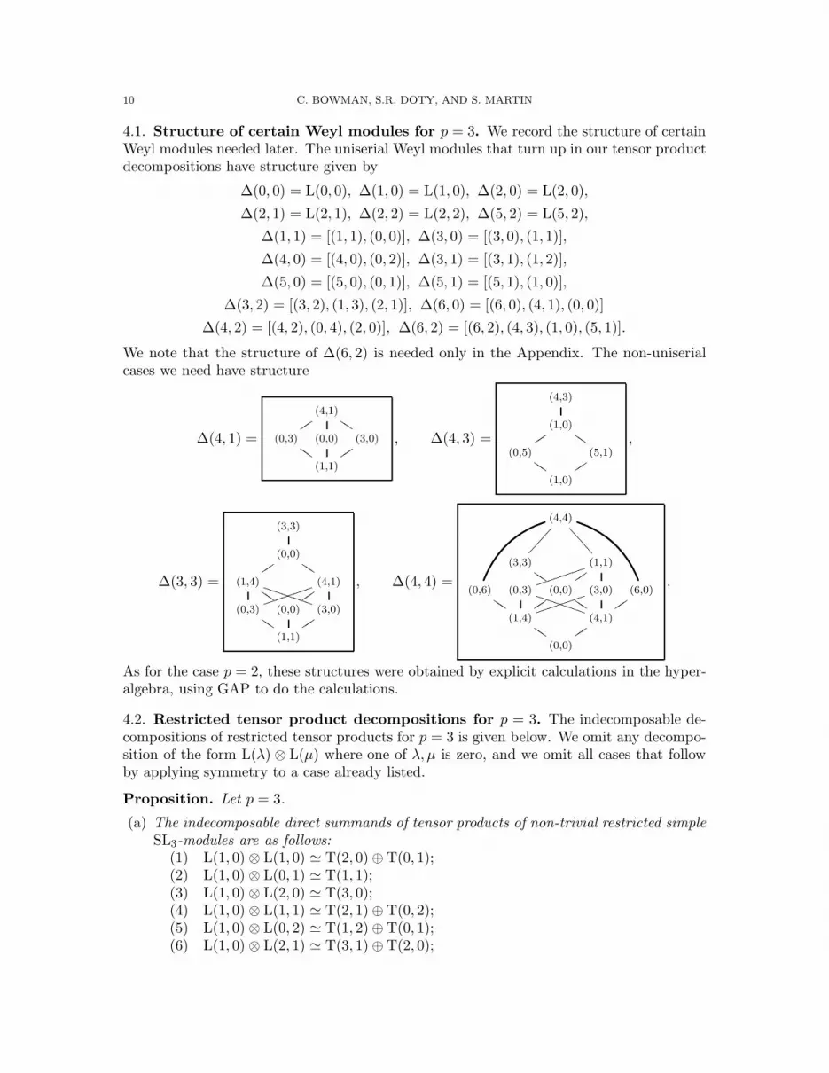
4.1. Structure of certain Weyl modules for p = 3. We record the structure of certainWeyl modules needed later. The uniserial Weyl modules that turn up in our tensor productdecompositions have structure given by
∆(0, 0) = L(0, 0), ∆(1, 0) = L(1, 0), ∆(2, 0) = L(2, 0),
∆(2, 1) = L(2, 1), ∆(2, 2) = L(2, 2), ∆(5, 2) = L(5, 2),
∆(1, 1) = [(1, 1), (0, 0)], ∆(3, 0) = [(3, 0), (1, 1)],
∆(4, 0) = [(4, 0), (0, 2)], ∆(3, 1) = [(3, 1), (1, 2)],
∆(5, 0) = [(5, 0), (0, 1)], ∆(5, 1) = [(5, 1), (1, 0)],
∆(3, 2) = [(3, 2), (1, 3), (2, 1)], ∆(6, 0) = [(6, 0), (4, 1), (0, 0)]
∆(4, 2) = [(4, 2), (0, 4), (2, 0)], ∆(6, 2) = [(6, 2), (4, 3), (1, 0), (5, 1)].
We note that the structure of ∆(6, 2) is needed only in the Appendix. The non-uniserialcases we need have structure
∆(4, 1) =
(4,1)
uuu III
(0,3)III(0,0) (3,0)
uuu
(1,1)
, ∆(4, 3) =
(4,3)
(1,0)
uuu III
(0,5)III
(5,1)
uuu
(1,0)
,
∆(3, 3) =
(3,3)
(0,0)
uuu III
(1,4)III
TTTTTTTT (4,1)
uuujjjjjjjj
(0,3)III(0,0) (3,0)
uuu
(1,1)
, ∆(4, 4) =
(4,4)
����
�
<<<<
<
(3,3)III
(1,1)
uuujjjjjjjj
(0,6)III(0,3)
TTTTTTTT (0,0)
uuu III(3,0)
jjjjjjjj (6,0)
uuu
(1,4)III
(4,1)
uuu
(0,0)
.
As for the case p = 2, these structures were obtained by explicit calculations in the hyper-algebra, using GAP to do the calculations.
4.2. Restricted tensor product decompositions for p = 3. The indecomposable de-compositions of restricted tensor products for p = 3 is given below. We omit any decompo-sition of the form L(λ) ⊗ L(µ) where one of λ, µ is zero, and we omit all cases that followby applying symmetry to a case already listed.
Proposition. Let p = 3.
(a) The indecomposable direct summands of tensor products of non-trivial restricted simpleSL3-modules are as follows:
(1) L(1, 0) ⊗ L(1, 0) ≃ T(2, 0)⊕ T(0, 1);(2) L(1, 0) ⊗ L(0, 1) ≃ T(1, 1);(3) L(1, 0) ⊗ L(2, 0) ≃ T(3, 0);(4) L(1, 0) ⊗ L(1, 1) ≃ T(2, 1)⊕ T(0, 2);(5) L(1, 0) ⊗ L(0, 2) ≃ T(1, 2)⊕ T(0, 1);(6) L(1, 0) ⊗ L(2, 1) ≃ T(3, 1)⊕ T(2, 0);

DECOMPOSITION OF TENSOR PRODUCTS 11
(7) L(1, 0) ⊗ L(1, 2) ≃ T(2, 2)⊕ T(0, 3);(8) L(1, 0) ⊗ L(2, 2) ≃ T(3, 2);(9) L(2, 0) ⊗ L(2, 0) ≃ T(4, 0)⊕ T(2, 1);(10) L(2, 0) ⊗ L(1, 1) ≃ T(3, 1) ⊕ T(0, 1);(11) L(2, 0) ⊗ L(0, 2) ≃ T(2, 2) ⊕ T(1, 1);(12) L(2, 0) ⊗ L(2, 1) ≃ T(4, 1) ⊕ T(2, 2);(13) L(2, 0) ⊗ L(1, 2) ≃ T(3, 2) ⊕ T(0, 2) ⊕ T(1, 0);(14) L(2, 0) ⊗ L(2, 2) ≃ T(4, 2) ⊕ T(2, 3);(15) L(1, 1) ⊗ L(1, 1) ≃ T(2, 2) ⊕ T(0, 0) ⊕M;(16) L(1, 1) ⊗ L(2, 1) ≃ T(3, 2) ⊕ T(4, 0) ⊕ T(1, 0);(17) L(1, 1) ⊗ L(2, 2) ≃ T(3, 3) ⊕ T(2, 2);(18) L(2, 1) ⊗ L(2, 1) ≃ T(4, 2) ⊕ T(5, 0) ⊕ T(2, 3)⊕ T(3, 1);(19) L(2, 1) ⊗ L(1, 2) ≃ T(3, 3) ⊕ 2T(2, 2) ⊕ T(1, 1);(20) L(2, 1) ⊗ L(2, 2) ≃ T(4, 3) ⊕ 2T(3, 2) ⊕ T(2, 4);(21) L(2, 2) ⊗ L(2, 2) ≃ T(4, 4) ⊕ T(3, 3) ⊕ T(5, 2)⊕ T(2, 5) ⊕ 3T(2, 2).
Thus the family F is in this case given by the twenty-five tilting modules {T(a, b) : 0 6
a, b 6 4} along with the six “exceptional” modules
{T(5, 0),T(0, 5),T(5, 2),T(2, 5),L(1, 1),M}.
All members of F except L(1, 1) and M are tilting modules.
(b) The uniserial members of F have the following structure:T(0, 0) = [(0, 0)]; T(1, 0) = [(1, 0)]; T(2, 0) = [(2, 0)];T(1, 1) = [(0, 0), (1, 1), (0, 0)]; T(2, 1) = [(2, 1)];T(4, 0) = [(0, 2), (4, 0), (0, 2)]; T(3, 1) = [(1, 2), (3, 1), (1, 2)];T(2, 2) = [(2, 2)]; T(5, 0) = [(0, 1), (5, 0), (0, 1)]; T(5, 2) = [(5, 2)].
The structure of the non-uniserial rigid members of F is given below (symmetric casesomitted):
(1,1)
uuu III
(3,0) (0,0)
(1,1)
III uuu
(1,1)IIIuuu
(3,0) (0,0) (0,3)
(1,1)
uuuIII
(2,1)
(1,3)
uuu III
(2,1)III
(3,2)
uuu
(1,3)
(2,1)
(1,1)
uuu III
(0,3)
uuu III(0,0)
jjjjjjjj (3,0)
uuu III
(1,1)III
(4,1)
uuu III(1,1)
uuujjjjjjjj
(3,0) (0,0) (0,3)
(1,1)
III uuu
(2,0)
(0,4)
uuu III
(2,0)III
(4,2)
uuu
(0,4)
(2,0)
all of which are tilting modules excepting the module M (which does not have a high-est weight) pictured at the upper right. Finally, there are four members of F, namelyT(3, 3), T(4, 3), T(3, 4), and T(4, 4), whose structure is not rigid, which are not pic-tured. Analysis of their structure requires other methods (see the Appendix).
(c) Each member of F except T(5, 2) = L(5, 2), T(2, 5) = L(2, 5) has simple G1T -socle(and head) of highest weight belonging to X1.

12 C. BOWMAN, S.R. DOTY, AND S. MARTIN
Remark. The Alperin diagram for T(4, 1) given above is one of several possibilities. Whena module has a direct sum of two or more copies of the same simple on a given socle layer,there may be more than one diagram.
The proof of the proposition will be given in 4.4–4.12. First we consider some conse-quences and look at a few examples.
Corollary. Let p = 3. Given arbitrary dominant weights λ, µ write λ =∑
λjpj , µ =∑µjpj with each λj , µj ∈ X1.
(a) In the decomposition (1.1.3), each term in the direct sum not involving a tensor factorof the form T(5, 2), T(2, 5) is indecomposable.
(b) L(λ) ⊗ L(µ) is indecomposable if and only if for each j > 0 the unordered pair{λj , µj} is one of the cases {(1, 0), (0, 1)], {(1, 0), (2, 0)], {(1, 0), (2, 2)], {(0, 1), (0, 2)],{(0, 1), (2, 2)] or one of λj, µj is the zero weight (0, 0).
(c) Let m be the maximum j such that at least one of λj , µj is non-zero. Then L(λ)⊗L(µ)is indecomposable tilting, isomorphic to T(λ+ µ), if and only if: (i) for each 0 6 j 6
m− 1, one of λj , µj is minuscule and the other is the Steinberg weight (2, 2), and (ii){λm, µm} is one of the cases listed in part (b).
Proof. The proof is entirely similar to the proof of the corresponding result in the p = 2case. We leave the details to the reader. �
Examples. (i) We work out the indecomposable direct summands of L(5, 4)⊗L(4, 5), usinginformation from part (a) of the proposition and following the procedure of Section 1.1:
L(5, 4) ⊗ L(4, 5)
≃(L(2, 1) ⊗ L(1, 1)[1]
)⊗
(L(1, 2) ⊗ L(1, 1)[1]
)
≃(L(2, 1) ⊗ L(1, 2)
)⊗
(L(1, 1) ⊗ L(1, 1)
)[1]
≃(T(3, 3) ⊕ 2T(2, 2) ⊕ T(1, 1)
)⊗
(T(2, 2) ⊕ T(0, 0) ⊕M
)[1]
≃(T(3, 3) ⊗ T(2, 2)[1]
)⊕
(T(3, 3)⊗ T(0, 0)[1]
)⊕(T(3, 3) ⊗M[1]
)
⊕ 2(T(2, 2) ⊗ T(2, 2)[1]
)⊕ 2
(T(2, 2) ⊗ T(0, 0)[1]
)⊕ 2
(T(2, 2) ⊗M[1]
)
⊕(T(1, 1) ⊗ T(2, 2)[1]
)⊕
(T(1, 1) ⊗ T(0, 0)[1]
)⊕
(T(1, 1) ⊗M[1]
)
≃ T(9, 9) ⊕ T(3, 3) ⊕(T(3, 3) ⊗M[1]
)⊕ 2T(8, 8) ⊕ 2T(2, 2)
⊕ 2(T(2, 2) ⊗M[1]
)⊕ T(7, 7) ⊕ T(1, 1)⊕
(T(1, 1) ⊗M[1]
).
We applied (2.4.4) to get the last line of the calculation.
(ii) Illustrating part (b) of the corollary we have L(3, 1) ⊗ L(1, 3) ≃ L(0, 1) ⊗ L(1, 0)[1] ⊗
L(1, 0) ⊗ L(0, 1)[1] ≃ T(1, 1)⊗ T(1, 1)[1] , which is indecomposable but not tilting.
(iii) To illustrate part (c) of the corollary we have for instance L(4, 0) ⊗ L(8, 8) ≃ T(12, 8)or L(5, 2) ⊗ L(5, 4) ≃ T(10, 6).
4.3. We now discuss the problem of computing the indecomposable direct summands (andtheir multiplicities) of L(λ)⊗L(µ) for arbitrary λ, µ ∈ X+, in the more difficult case wherea direct summand on the right hand side of (1.1.3) is not necessarily indecomposable.

DECOMPOSITION OF TENSOR PRODUCTS 13
It will be convenient to introduce the notation F0 for the set F−{T(5, 2),T(2, 5)}. Then
Corollary 4.2(a) says that a direct summand S =⊗
j>0 I[j]j in (1.1.3) is indecomposable
whenever all its tensor factors Ij belong to F0.
Consider a summand S =⊗
j>0 I[j]j in (1.1.3) which is possibly not indecomposable. By
Corollary 4.2(a), such a summand must have one or more tensor multiplicands of the formT(5, 2) or T(2, 5). Suppose that in the summand in question Ik is T(5, 2) or T(2, 5). We
use the fact that T(5, 2) = L(5, 2) ≃ L(2, 2) ⊗ L(1, 0)[1], and similarly T(2, 5) = L(2, 5) ≃L(2, 2)⊗L(0, 1)[1]. Thus we are forced to consider the possible splitting of L(1, 0)⊗ Ik+1 orL(0, 1)⊗ Ik+1 in ‘degree’ k+1. (By ‘degree’ here we just mean the level of j in the twistedtensor product occurring in a direct summand of the right-hand-side of (1.1.3).) There aretwo cases.
We consider first the case where Ik+1 is not tilting, i.e., Ik+1 is either L(1, 1) or M. Sowe need to split L(1, 0)⊗L(1, 1), L(0, 1)⊗L(1, 1), L(1, 0)⊗M or L(0, 1)⊗M. The first twocases are already covered by Corollary 4.2(a), so we just need to consider the last two. Buta simple calculation with characters and consideration of linkage classes shows that
(4.3.1)L(1, 0) ⊗M ≃ T(3, 1)⊕ T(1, 0) ⊕ T(4, 0);
L(0, 1) ⊗M ≃ T(1, 3) ⊕ T(0, 1) ⊕ T(0, 4)
and the summands are once again members of F with restricted socles, so these cases presentno problem.
We are left with the case where Ik+1 is tilting. Then this splitting can be computedsince L(1, 0) = T(1, 0) and L(0, 1) = T(0, 1) are tilting, so we are just splitting a tensorproduct of two tilting modules into a direct sum of indecomposable tilting modules, whichcan always be done. This new decomposition produces only tilting modules in the familyF except when Ik+1 is one of the following cases:
T(5, 0),T(4, 1),T(4, 2),T(5, 2),T(4, 3), and T(4, 4)
or one of their symmetric cousins. Up to lower order terms which again belong to F, thesepossibilities, when tensored by L(1, 0) or L(0, 1), produce the new tilting modules
(4.3.2) T(6, 0),T(5, 1),T(6, 2),T(5, 3), and T(5, 4)
and of course their symmetric versions. Now by Donkin’s tensor product theorem we havea twisted tensor product decomposition for the last three of these, in terms of members ofF:
(4.3.3)
T(6, 2) ≃ T(3, 2) ⊗ T(1, 0)[1],
T(5, 3) ≃ T(2, 3) ⊗ T(1, 0)[1],
T(5, 4) ≃ T(2, 4) ⊗ T(1, 0)[1].
Hence, those summands and their symmetric versions present no problem. Finally, if T(5, 0)or T(4, 1) is tensored by L(1, 0) then, modulo lower order terms which belong to F, weobtain the new summands T(6, 0) and T(5, 1) which are not members of F and do notadmit a twisted tensor product decomposition. However, these summands must have simplerestricted G1T -socles, since they are embedded in T(4, 4) and T(4, 3), respectively. This isshown by translation arguments, similar to those in 4.12 ahead. Thus we have proved thefollowing result.

14 C. BOWMAN, S.R. DOTY, AND S. MARTIN
Proposition. Let p = 3 and G = SL3.
(a) Any tensor product of the form L(1, 0)⊗ I or L(0, 1)⊗ I, where I is an indecomposabletilting module in F, is expressible as a twisted tensor product of modules which areeither tilting modules in F0 or are one of the “extra” modules T(6, 0), T(5, 1), T(0, 6)or T(1, 5).
(b) The extra modules have simple restricted G1T -socles.
(c) For general λ, µ ∈ X+, the indecomposable direct summands of L(λ) ⊗ L(µ) are allexpressible as twisted tensor products of modules from the family
F′ = F0 ∪ {T(6, 0),T(5, 1),T(0, 6),T(1, 5)}
= {T(a, b) : 0 6 a, b 6 4} ∪
{T(6, 0),T(5, 1),T(5, 0),T(0, 6),T(1, 5),T(0, 5),L(1, 1),M}.
Note that all members of F′ have simple G1T -socle of restricted highest weight.
Example. We consider an example where the direct summands on the right hand side of(1.1.3) are not all indecomposable:
L(2, 2) ⊗ L(5, 2) ≃ L(2, 2) ⊗ L(2, 2) ⊗ L(1, 0)[1]
≃(T(4, 4)⊕ T(3, 3) ⊕ T(5, 2) ⊕ T(2, 5) ⊕ 3T(2, 2)
)⊗ L(1, 0)[1]
≃ T(7, 4) ⊕ T(6, 3) ⊕T(8, 2) ⊕ T(2, 5) ⊕ T(5, 5) ⊕ 3T(5, 2).
The second line comes from equation (21) in Proposition 4.2(a), and to get the last line oneapplies (2.4.4) repeatedly, using Proposition 4.2(a) again as needed. For instance, usingequation (1) from Proposition 4.2(a) we have
T(5, 2) ⊗ L(1, 0)[1] ≃ L(2, 2) ⊗(L(1, 0) ⊗ L(1, 0)
)[1]
≃ L(2, 2) ⊗(T(2, 0) ⊕ T(0, 1)
)[1]
≃ T(8, 2)⊕ T(2, 5)
and using equation (2) from Proposition 4.2(a) we have
T(2, 5) ⊗ L(1, 0)[1] ≃ L(2, 2) ⊗(L(0, 1) ⊗ L(1, 0)
)[1]
≃ L(2, 2) ⊗ T(1, 1)[1] ≃ T(5, 5).
4.4. We now embark upon the proof of Proposition 4.2. First we compute the compositionfactor multiplicities of the restricted tensor products. (Recall that χp(λ) = L(λ) is theformal character of L(λ).)
(1) χp(1, 0) · χp(1, 0) = χp(2, 0) + χp(0, 1);(2) χp(1, 0) · χp(0, 1) = χp(1, 1) + 2χp(0, 0);(3) χp(1, 0) · χp(2, 0) = χp(3, 0) + 2χp(1, 1) + χp(0, 0);(4) χp(1, 0) · χp(1, 1) = χp(2, 1) + χp(0, 2);(5) χp(1, 0) · χp(0, 2) = χp(1, 2) + χp(0, 1);(6) χp(1, 0) · χp(2, 1) = χp(3, 1) + 2χp(1, 2) + χp(2, 0);(7) χp(1, 0) · χp(1, 2) = χp(2, 2) + χp(0, 3) + 2χp(1, 1) + χp(0, 0);(8) χp(1, 0) · χp(2, 2) = χp(3, 2) + 2χp(1, 3) + 3χp(2, 1);(9) χp(2, 0) · χp(2, 0) = χp(4, 0) + χp(2, 1) + 2χp(0, 2);
(10) χp(2, 0) · χp(1, 1) = χp(3, 1) + 2χp(1, 2) + χp(0, 1);
DECOMPOSITION OF TENSOR PRODUCTS 15
(11) χp(2, 0) · χp(0, 2) = χp(2, 2) + χp(1, 1) + 2χp(0, 0);(12) χp(2, 0) ·χp(2, 1) = χp(4, 1) +χp(2, 2) + 2χp(0, 3) + 2χp(3, 0) + 4χp(1, 1) + 2χp(0, 0);(13) χp(2, 0) · χp(1, 2) = χp(3, 2) + 2χp(1, 3) + 3χp(2, 1) + χp(0, 2) + χp(1, 0);(14) χp(2, 0) ·χp(2, 2) = χp(4, 2) +χp(2, 3) + 2χp(0, 4) + 2χp(3, 1) + 3χp(1, 2) + 3χp(2, 0);(15) χp(1, 1) · χp(1, 1) = χp(2, 2) + χp(0, 3) + χp(3, 0) + 2χp(1, 1) + 2χp(0, 0);(16) χp(1, 1) · χp(2, 1) = χp(3, 2) + 2χp(1, 3) + χp(4, 0) + 3χp(2, 1) + 2χp(0, 2) + χp(1, 0);(17) χp(1, 1) ·χp(2, 2) = χp(3, 3)+2χp(1, 4)+2χp(4, 1)+χp(2, 2)+4χp(0, 3)+4χp(3, 0)+
6χp(1, 1) + 5χp(0, 0);(18) χp(2, 1) ·χp(2, 1) = χp(4, 2)+χp(2, 3)+ 2χp(0, 4)+χp(5, 0)+ 3χp(3, 1)+ 5χp(1, 2)+
3χp(2, 0) + 2χp(0, 1);(19) χp(2, 1) ·χp(1, 2) = χp(3, 3)+2χp(1, 4)+2χp(4, 1)+2χp(2, 2)+4χp(0, 3)+4χp(3, 0)+
7χp(1, 1) + 7χp(0, 0);(20) χp(2, 1) ·χp(2, 2) = χp(4, 3)+χp(2, 4)+2χp(0, 5)+2χp(5, 1)+2χp(3, 2)+4χp(1, 3)+
2χp(4, 0) + 6χp(2, 1) + 3χp(0, 2) + 5χp(1, 0);(21) χp(2, 2) ·χp(2, 2) = χp(4, 4)+χp(2, 5)+ 2χp(0, 6)+χp(5, 2)+ 3χp(3, 3)+ 6χp(1, 4)+
2χp(6, 0) + 6χp(4, 1) + 3χp(2, 2) + 8χp(0, 3) + 8χp(3, 0) + 11χp(1, 1) + 15χp(0, 0).
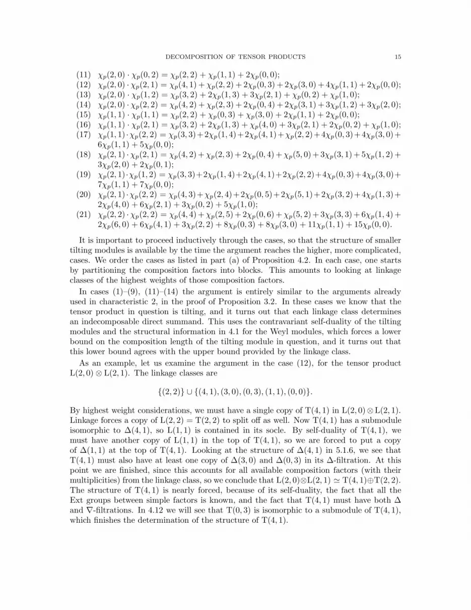
It is important to proceed inductively through the cases, so that the structure of smallertilting modules is available by the time the argument reaches the higher, more complicated,cases. We order the cases as listed in part (a) of Proposition 4.2. In each case, one startsby partitioning the composition factors into blocks. This amounts to looking at linkageclasses of the highest weights of those composition factors.
In cases (1)–(9), (11)–(14) the argument is entirely similar to the arguments alreadyused in characteristic 2, in the proof of Proposition 3.2. In these cases we know that thetensor product in question is tilting, and it turns out that each linkage class determinesan indecomposable direct summand. This uses the contravariant self-duality of the tiltingmodules and the structural information in 4.1 for the Weyl modules, which forces a lowerbound on the composition length of the tilting module in question, and it turns out thatthis lower bound agrees with the upper bound provided by the linkage class.
As an example, let us examine the argument in the case (12), for the tensor productL(2, 0) ⊗ L(2, 1). The linkage classes are
{(2, 2)} ∪ {(4, 1), (3, 0), (0, 3), (1, 1), (0, 0)}.
By highest weight considerations, we must have a single copy of T(4, 1) in L(2, 0)⊗L(2, 1).Linkage forces a copy of L(2, 2) = T(2, 2) to split off as well. Now T(4, 1) has a submoduleisomorphic to ∆(4, 1), so L(1, 1) is contained in its socle. By self-duality of T(4, 1), wemust have another copy of L(1, 1) in the top of T(4, 1), so we are forced to put a copyof ∆(1, 1) at the top of T(4, 1). Looking at the structure of ∆(4, 1) in 5.1.6, we see thatT(4, 1) must also have at least one copy of ∆(3, 0) and ∆(0, 3) in its ∆-filtration. At thispoint we are finished, since this accounts for all available composition factors (with theirmultiplicities) from the linkage class, so we conclude that L(2, 0)⊗L(2, 1) ≃ T(4, 1)⊕T(2, 2).The structure of T(4, 1) is nearly forced, because of its self-duality, the fact that all theExt groups between simple factors is known, and the fact that T(4, 1) must have both ∆and ∇-filtrations. In 4.12 we will see that T(0, 3) is isomorphic to a submodule of T(4, 1),which finishes the determination of the structure of T(4, 1).

16 C. BOWMAN, S.R. DOTY, AND S. MARTIN
4.5. In case (10), one cannot immediately conclude that L(2, 0) ⊗ L(1, 1) is tilting sinceL(1, 1) is not tilting, so we must proceed differently. However, we observe the following,which immediately implies that in fact our tensor product is tilting.
Lemma. Let V be a simple Weyl module and let ∆(λ) be a Weyl module of highest weightλ. If the composition factors of V ⊗ rad∆(λ) and V ⊗ L(λ) lie in disjoint blocks, thenV ⊗ L(λ) is tilting.
Proof. V ⊗∆(λ) has a ∆-filtration, by the Wang–Donkin–Mathieu result (see [17, II.4.21]).Now as V ⊗ rad∆(λ) and V ⊗ L(λ) have no common linkage classes there can be nonon-trivial extensions between these modules, by the linkage principle. Thus V ⊗∆(λ) =(V ⊗ rad∆(λ)
)⊕
(V ⊗ L(λ)
). As V ⊗∆(λ) has a ∆-filtration this implies V ⊗ L(λ) does
also. As it is the tensor product of two simple (therefore contravariantly self dual) modulesit is itself contravariantly self dual and so has a ∇-filtration. Therefore it is tilting. �
Now we may proceed as usual. Looking at the character of L(2, 0) ⊗ L(1, 1) we findthat there are two linkage classes for the highest weights of the composition factors, namely{(0, 1)} and {(3, 1), (1, 2)}. Since the multiplicity of L(0, 1) is 1, it must give a simple tiltingsummand T(0, 1). Now T(3, 1) must be a summand by highest weight consideration, andthe usual argument forces it to have at least composition length three, which forces equalityof the upper and lower bounds, so the structure is T(3, 1) = [(1, 2), (3, 1), (1, 2)] and we haveL(2, 0) ⊗ L(1, 1) ≃ T(3, 1) ⊕ T(0, 1). This takes care of case (10) in our list.
Case (16) follows similarly, making use again of the above lemma to conclude thatL(1, 1) ⊗ L(2, 1) is tilting. We note that at this stage we may assume that the struc-ture of T(3, 2) and T(4, 0) are already known, since they come up in the earlier cases (8),(9). So one easily concludes from this and the linkage classes that L(1, 1) ⊗ L(2, 1) ≃T(3, 2) ⊕ T(4, 0) ⊕T(1, 0).
4.6. We now consider case (15). Since L(1, 1) is not tilting, it is unclear whether or notL(1, 1)⊗ L(1, 1) is tilting. In fact it is not, and analysis of this case is more difficult. First,looking at the character and the linkage classes (there are two) we observe that a copyof the Steinberg module T(2, 2) = L(2, 2) splits off as a direct summand. The remainingcomposition factors of the tensor product all lie in the same linkage class, but it turns outthat a copy of the trivial module splits off, as we show below.
From properties of duals and previous calculations it follows that
(1)
dimK HomG(L(0, 0),L(1, 1) ⊗ L(1, 1))
= dimK HomG(L(0, 0) ⊗ L(1, 1),L(1, 1))
= dimK HomG(L(1, 1),L(1, 1)) = 1;
(2)
dimK HomG(T(1, 1),L(1, 1) ⊗ L(1, 1))
= dimK HomG(L(1, 0) ⊗ L(0, 1),L(1, 1) ⊗ L(1, 1))
= dimK HomG(L(1, 1) ⊗ L(0, 1),L(1, 1) ⊗ L(0, 1))
= dimK HomG(L(1, 2) ⊕ L(2, 0),L(1, 2) ⊕ L(2, 0)) = 2;

DECOMPOSITION OF TENSOR PRODUCTS 17
(3)
dimK HomG(L(3, 0),L(1, 1) ⊗ L(1, 1))
= dimK HomG(L(1, 1) ⊗ L(3, 0),L(1, 1))
= dimK HomG(L(4, 1),L(1, 1)) = 0
and, by symmetry, an equality similar to (3) holds, in which (3, 0) is replaced by (0, 3). Wealso observe that
(4) HomG(L(1, 1),L(1, 1) ⊗ L(1, 1)) ≃ HomG(L(1, 1) ⊗ L(1, 1),L(1, 1))
By (1), (3), and (4) we see that the socle of L(1, 1)⊗ L(1, 1) is either: (a) L(2, 2)⊕ L(0, 0),or (b) L(2, 2) ⊕ L(0, 0) ⊕ L(1, 1).
From the structure of the Weyl modules in question we know (see e.g. [17, II.4.14]) all theExt1 groups between the simple modules of interest here. Combining this with self-dualitywould force the structure of the non-simple direct summand of L(1, 1)⊗L(1, 1) to be givenby one of the following diagrams:
(0,0)
(1,1)IIIuuu
(3,0) (0,3)
(1,1)
uuuIII
(0,0)
(1,1)IIIuuu
(3,0) (0,0) (0,3)
(1,1)
uuuIII
where the left diagram corresponds with possibility (a) and the right with possibility (b).However, the left diagram would contradict (2). Hence, possibility (a) is in fact ruled out,and we are left with possibility (b). It follows that L(1, 1)⊗L(1, 1) ≃ L(2, 2)⊕L(0, 0)⊕M,as claimed.
4.7. There are just five cases remaining in the proof of Proposition 4.2, namely cases (17)–(21). We now consider case (17). The module L(1, 1) ⊗ L(2, 2) is tilting by Lemma 4.5,so by highest weight considerations T(3, 3) is a direct summand. This is also justified byPillen’s Theorem (see 2.1). The character of T(3, 3) may be computed by (2.2.2), whichshows that it has a ∆-filtration with ∆-factors isomorphic to
∆(3, 3), ∆(4, 1), ∆(1, 4), ∆(3, 0), ∆(0, 3), ∆(1, 1)
each occurring with multiplicity one. This accounts for all the composition factors appearingin the character of L(1, 1)⊗ L(2, 2), except for one copy of the Steinberg module T(2, 2) =L(2, 2). Hence we conclude that
L(1, 1) ⊗ L(2, 2) ≃ T(3, 3) ⊕ T(2, 2).
4.8. L(2, 1) ⊗ L(2, 1) is tilting since L(2, 1) is, so by highest weight considerations a copyof T(4, 2) splits off as a direct summand. The structure of T(4, 2) was determined in aprevious case of the proof. Subtracting its character from the character of L(2, 1)⊗L(2, 1),we see that the highest weight of what remains is (5, 0), so a copy of T(5, 0) must split offas well. The linkage class of (5, 0) contains only two weights {(5, 0), (0, 1)} and from thisand the known structure of the Weyl modules it follows easily that T(5, 0) is uniserial with
18 C. BOWMAN, S.R. DOTY, AND S. MARTIN
structure T(5, 0) = [(0, 1), (5, 0), (0, 1)]. Now highest weight and character considerationsforce the remaining summands to be one copy of T(2, 3) and one copy of T(3, 1). Hence
L(2, 1) ⊗ L(2, 1) ≃ T(4, 2) ⊕ T(5, 0) ⊕ T(2, 3) ⊕ T(3, 1).
We note we can assume that T(3, 1) and T(2, 3) are known at this point, since they arise inearlier cases of the proof. (Actually, to be precise T(2, 3) doesn’t arise in any earlier case,but its symmetric cousin T(3, 2) does.)
4.9. L(2, 1) ⊗ L(1, 2) is tilting since both L(2, 1) and L(1, 2) are, so by highest weightconsiderations a copy of T(3, 3) splits off as a direct summand. The character of T(3, 3)was computed already in 4.7, so by character considerations one easily deduces that
L(2, 1) ⊗ L(1, 2) ≃ T(3, 3) ⊕ 2T(2, 2) ⊕ T(1, 1).
Of course, the character of T(1, 1) is already known by an earlier case of the proof.
4.10. L(2, 1) ⊗ L(2, 2) is tilting since both L(2, 1) and L(2, 2) are, so by highest weightconsiderations a copy of T(4, 3) splits off as a direct summand. From [8, §2.1, Lemma 5]we compute its ∆-factors to be
∆(4, 3), ∆(5, 1), ∆(0, 5), ∆(1, 0).
One sees also that T(4, 3) has simple socle of highest weight (1, 0) by arguments similar tothose in 4.7. From character computations one now shows that
L(2, 1) ⊗ L(2, 2) ≃ T(4, 3) ⊕ 2T(3, 2) ⊕ T(2, 4).
The structure of T(3, 2) is available by a previous case of the proof, and the structure ofT(2, 4) follows by symmetry from that of T(4, 2), again a previous case.
4.11. L(2, 2)⊗L(2, 2) is tilting since L(2, 2) is, so by highest weight considerations a copyof T(4, 4) must split off as a direct summand. The ∆-factor multiplicities of T(4, 4) arecomputed by [8, §2.1, Lemma 5] to be
∆(4, 4), ∆(6, 0), ∆(0, 6), ∆(3, 3), ∆(4, 1), ∆(1, 4), ∆(1, 1), ∆(0, 0)
each of multiplicity one. From this, using the character of L(2, 2) ⊗ L(2, 2) it follows byhighest weight considerations, after subtracting the character of T(4, 4), that a copy ofT(3, 3) must also split off as a direct summand. Then it easily follows that
L(2, 2) ⊗ L(2, 2) ≃ T(4, 4) ⊕ T(3, 3) ⊕T(5, 2) ⊕ T(2, 5) ⊕ 3T(2, 2)
where T(5, 2) = L(5, 2), T(2, 5) = L(2, 5), and T(2, 2) = L(2, 2).
At this point the proof of Proposition 4.2(a), (b) is complete.
4.12. It remains to prove the claim in part (c) of Proposition 4.2. It is known that Donkin’sconjecture holds for SL3, as discussed at the beginning of 2.4, so T((p − 1)ρ + λ) is as a
G1T -module isomorphic to Q1((p − 1)ρ + w0λ) for any λ ∈ X1. Thus T(a, b) has simpleG1T -socle of restricted highest weight, for any 2 6 a, b 6 4. Moreover, the claim is true ofT(0, 0), T(1, 0), T(2, 0), T(2, 1), L(1, 1) and their symmetric counterparts, since these areall simple G-modules of restricted highest weight.
For λ = (1, 1) and (5, 0) one easily checks by direct computation that ∆(λ), which is anon-split extension between two simple G-modules, remains non-split upon restriction toG1T . It then follows that T(λ) has simple G1T -socle of restricted highest weight in eachcase.

DECOMPOSITION OF TENSOR PRODUCTS 19
For λ = (4, 0) and (3, 1) one could argue as in the preceding paragraph, or restrict to anappropriate Levi subgroup, as in the last paragraph of 3.3.
The remaining cases, up to symmetry, are T(3, 0), T(4, 1), and M. We apply the trans-lation principle [17, II.E.11]. Observe (from their structure) that T(0, 2) embeds in T(4, 0),which in turn embeds in T(2, 4). Picking λ = (0, 0) and µ = (−1, 1) in the closure of thebottom alcove, observe that applying the (exact) functor T λ
µ to these embeddings, we obtainembeddings of T(0, 3) in T(4, 1), and T(4, 1) in T(3, 3). Since T(3, 3) has simple G1T -socleof restricted highest weight, it follows that the same holds for T(0, 3) and T(4, 1). Thecases T(3, 0) and T(1, 4) are treated by the symmetric argument. Finally, we observe thatdimK HomG1T (L(0, 0),L(1, 1) ⊗ L(1, 1)) = 1, by a calculation similar to 4.6(1). This, alongwith 4.6, shows that M remains indecomposable on restriction to G1T , with socle and headisomorphic to L(1, 1), and with 7 copies of L(0, 0) in the middle Loewy layer. The proof ofProposition 4.2 is complete.
4.13. Discussion. We now discuss the remaining issue in characteristic 3: the structure ofthe tilting modules T(λ) for λ = (3, 3), (4, 3), (3, 4), and (4, 4). These tilting modules are infact S-modules for the Schur algebra S = SK(3, r) in degree r = 9, 10, 11, 12, respectively.(See [13, 20] for background on Schur algebras.)
Thus, in order to study the structure of T(λ) one may employ techniques from thetheory of finite dimensional quasi-hereditary algebras. Now the simplest cases (in terms ofnumber of composition factors) are T(4, 3) for S(3, 10) and T(3, 4) for S(3, 11). As thesemodules are symmetric, it makes sense to focus on the smaller Schur algebra S(3, 10) andthus T(4, 3). In fact, it is enough to understand the block A of S(3, 10) consisting of thesix weights (10, 0), (6, 2), (4, 3), (5, 1), (0, 5), and (1, 0). (It is easily seen that this is acomplete linkage class of dominant weights in S(3, 10), for instance by drawing the alcovediagrams.) To construct T(4, 3) we must “glue” together the ∆-factors in a way that resultsin a contravariantly self-dual module. Looking at the diagrams in Figure 1 below picturing
(1,0)
(0,5) (5,1)
(1,0) (1,0)
(4,3)
(1,0)
uuu III
(0,5)III
(5,1)
uuu
(1,0)
Figure 1. Weyl filtration factors of T(4, 3)
the various Weyl modules in the filtration, we see that it is impossible to do this in a rigidway. There are three copies of L(1, 0) above the middle factor L(4, 3) and only two below.Thus, there must be two copies of L(1, 0) lying immediately above L(4, 3) when viewing theradical series, and two copies lying immediately below L(4, 3) when viewing the socle series.This implies that T(4, 3) is not rigid. To understand the structure of T(4, 3) one may apply

20 C. BOWMAN, S.R. DOTY, AND S. MARTIN
Gabriel’s theorem to find a quiver and relations presentation for the basic algebra of theblock A, or an appropriate quasi-hereditary quotient thereof. This is carried out in theAppendix. The other cases could be treated similarly.
Note that none of T(4, 3), T(3, 4), T(3, 3), or T(4, 4) is projective as an S-module, becauseif so, the reciprocity law (P (λ) : ∆(µ)) = [∇(µ) : L(λ)] (see e.g. [6, Prop. A2.2]) would beviolated.
References
[1] J.L. Alperin, Diagrams for modules, J. Pure Appl. Algebra 16 (1980), 111–119.[2] H.H. Andersen and M. Kaneda, Rigidity of tilting modules, preprint.[3] S. Donkin, On Schur algebras and related algebras I, J. Algebra 104 (1986), 310–328.[4] S. Donkin, On Schur algebras and related algebras II, J. Algebra 111 (1987), 354–364.[5] S. Donkin, On tilting modules for algebraic groups, Math. Z. 212 (1993), 39–60.[6] S. Donkin, The q-Schur algebra, London Math. Soc. Lecture Note Ser., 253, Cambridge Univ.
Press 1998.[7] S. Donkin, Tilting modules for algebraic groups and finite dimensional algebras, Handbook of
Tilting Theory, 215–257, London Math. Soc. Lecture Note Ser., 332, Cambridge Univ. Press,Cambridge 2007.
[8] S. Donkin, The cohomology of line bundles on the three-dimensional flag variety, J. Algebra307 (2007), 570–613.
[9] S.R. Doty, The submodule structure of certain Weyl modules for groups of type An, J.Algebra 95 (1985), 373–383.
[10] S.R. Doty and J.B. Sullivan, Filtration patterns for representations of algebraic groups andtheir Frobenius kernels, Math. Z. 195 (1987), 391–407.
[11] S.R. Doty and A.E. Henke, Decomposition of tensor products of modular irreducibles forSL2, Quart. J. Math. 56 (2005), 189–207.
[12] GAP: Groups, Algorithms, Programming - a System for Computational Discrete Algebra,http://www.gap-system.org.
[13] J.A. Green, Polynomial Representations of GLn, second corrected and augmented edition,Lecture Notes in Mathematics 830, Springer, Berlin, 2007.
[14] R.S. Irving, The structure of certain highest weight modules for SL3, J. Algebra 99 (1986),438–457.
[15] J.C. Jantzen, Darstellungen halbeinfacher Gruppen und kontravariante Formen, J. reineangew. Math. 290 (1977), 117–141.
[16] J.C. Jantzen, Weyl modules for groups of Lie type, Finite Simple Groups II (Proc. Durham1978), Academic Press, London/New York (1980), 291–300.
[17] J.C. Jantzen, Representations of Algebraic Groups, (2nd ed.), Mathematical Surveys andMonographs 107, Amer. Math. Soc., Providence 2003.
[18] J. G. Jensen, On the character of some modular indecomposable tilting modules for SL3, J.Algebra 232 (2000), 397–419.
[19] K. Kuhne-Hausmann, Zur Untermodulstruktur der Weylmoduln fur SL3, Bonner Math.Schriften, 162, Univ. Bonn, Mathematisches Institut, Bonn 1985.
[20] S. Martin, Schur Algebras and Representation Theory, Cambridge Tracts in Math., vol. 112,Cambridge Univ. Press, Cambridge 1993.
[21] C. Pillen, Tensor products of modules with restricted highest weight, Commun. Algebra 21(1993), 3647–3661.
[22] N. Xi, Maximal and primitive elements in Weyl modules for type A2, J. Algebra 215 (1999),735–756.

APPENDIX: THE SL3-MODULE T (4, 3) FOR p = 3
C. M. Ringel
Let k be an algebraically closed field of characteristic p = 3. Following Bowman, Doty andMartin, we consider rational SL3-modules with composition factors L(λ), where λ is one ofthe weights (1, 0), (0, 5), (5, 1), (4, 3), (6, 2). Dealing with a dominant weight (a, b), or thesimple module L(a, b), we usually will write just ab. The corresponding Weyl module, dualWeyl module, or tilting module, will be denoted by ∆(ab), ∇(ab) and T (ab), respectively.
The paper [BDM] by Bowman, Doty and Martin describes in detail the structure ofthe modules ∆(λ),∇(λ) for λ = 10, 05, 51, 43, 62 and also T (10), T (05), T (51) and itprovides the factors of a ∆-filtration for T (43). This module T (43) is still quite small (ithas length 10), but its structure is not completely obvious at first sight. The main aim ofthis appendix is to explain the shape of this module.
Let us call a finite set I of dominant weights (or of simple modules) an ideal providedfor any λ ∈ I all composition factors of T (λ) belong to I. The category of modules with allcomposition factors in an ideal I is a highest weight category with weight set I, thus can beidentified with the module category of a basic quasi-hereditary algebra which we denote byA(I). In order to analyse the module T (43), we need to look at the ideal I = {10, 05, 51, 43},thus at the algebra A(10, 05, 51, 43).
In order to determine the precise relations for A(10, 05, 51, 43), we will have to look alsoat the module T (62), see section 4. Note that {10, 05, 51, 43, 62} is again an ideal, thuswe deal with the algebra A(10, 05, 51, 43, 62).
The use of quivers and relations for presenting a basic finite dimensional algebras wasinitiated by Gabriel around 1970, the text books [ARS] and [ASS] can be used as a reference.The class of quasi-hereditary algebras was introduced by Scott and Cline-Parshall-Scott;for basic properties one may refer to [DR] and [R2]. The author is grateful to S. Dotyand R. Farnsteiner for fruitful discussions and helpful suggestions concerning the materialpresented in the appendix.
1. The main result
Deviating from [BDM], we will consider right modules. Thus, given a finite-dimensionalalgebra A, an indecomposable projective A-module is of the form eA with e a primitiveidempotent. The algebras to be considered will be factor algebras of path algebras of quiversand the advantage of looking at right modules will be that in this way we can write thepaths in the quiver as going from left to right.
Proposition. The algebra A(10, 05, 51, 43) is isomorphic to the path algebra of the quiver
Q = Q(10, 05, 51, 43) 10
05
51
43................................................................................................................
............
................................................................................................................
............
....................................................................
............
....................................................................
............
....................................................................
.
..
.
..
.
.
.
.
.
.
....................................................................
.
..
.
.
..
.
.
.
.
.
αα′
β′β
γ
γ′

2222 C.M. RINGEL
modulo the ideal generated by the following relations
α′α = 0, α′β = 0, β′α = 0, β′(1− γγ′)β = 0,γ′γ = 0, γ′(αα′ − ββ′) = 0, (αα′ − ββ′)γ = 0, γ′αα′γ = 0.
We are going to give some comments before embarking on the proof.
(1) Since the quiver Q(10, 05, 51, 43) is bipartite, say with a (+)-vertex 10 and three (−)-vertices 05, 51, 43, possible relations between vertices of the same parity involve paths ofeven lengths, those between vertices with different parity involve paths of odd lengths. Ourconvention for labelling arrows between a (+)-vertex a and a (−)-vertex b is the following:we use a greek letter for the arrow a → b and add a dash for the arrow b → a.
(2) The assertion of the proposition can be visualized by drawing the shape of the in-decomposable projective A-modules. The indecomposable projective A-module with top λwill be denoted by P (λ) = eλA, where eλ is the primitive idempotent corresponding to λ,and we will denote the radical of A by J .
.
.
.
.
.
.
.
.
.
.
.
.
.
.
.
.
.
.
05
10
51
10.................
.................
43.........
10.................
.................
.................
.................
.
..
.
.
.
..
.
.
.
.
.
.
.
.
.
.
.
.
.
.
.
.
.
.
.
.
.
.
.
.
.
.
.
.
.
.
.
.
.
.
.
.
.
.
.
.
.
.
.
.
.
.
.
.
.
.
.
.
.
.
.
.
.
.
.
.
.
.
.
.
.
.
.
.
.
.
.
.
.
.
.
.
.
.
.
.
.
.
.
.
.
.
.
.
.
.
.
.
.
..
05 51
10
43
10
05 51
10
.
.
.
.
.
.
.
.
.
.
..
..
.
......
.
..
.........
............
..
.
.........
.
.
.
.
.
.
.
.
.
.....................................................
...................................................................
10
............
..
.
.........
05
10
43
10
05 51
.
.
.
.
.
.
.
.
.
.
.
.
.
.
.
.
.
.
.
.
.
.
.
.
.
.
.
.
...........
.
..
.........
10
..
.
.........
............
51
10
43
10
05 51
.
.
.
.
.
.
.
.
.
.
.
.
.
.
.
.
.
.
.
.
.
.
.
.
.
.
.
..
..
..
.
.
..
.
.
.
.
..
.
.
.
.
.
.
.
.
.
.
.
.
.
.
.
.
.
.
.
.
.
.
.
.
.
.
.
.
.
.
.
.
.
.
.
.
.
.
.
.
.
.
.
.
.
.
.
.
.
.
.
.
.
.
.
.
.
.
.
.
.
.
.
.
.
.
.
.
.
.
.
.
.
.
.
.
.
.
.
.
.
.
.
.
.
.
.
.
.
.
.
.
.
.
.
.
.
.
.
.
.
.
.
.
..
.........
.
..
..
..
.
..
..
10
43
10
05 51
10
.
...........
.
..
.
..
..
..
.
.
............
..
..........
.
.
.
.
.
.
.
.
.
These are the coefficient quivers of the indecomposable projective A-modules with respectto suitable bases. In addition, the proposition asserts that all the non-zero coefficents canbe chosen to be equal to 1. Note that this means that A has a basis B which consists ofa complete set of primitive and orthogonal idempotents as well as of elements from theradical J , and such that B is multiplicative (this means: if u, v ∈ B, then either uv = 0 orelse uv ∈ B).
For the convenience of the reader, let us recall the notion of a coefficient quiver (see forexample [R3]): By definition, a representation M of a quiver Q over a field k is of theform M = (Mx;Mα)x,α; here, for every vertex x of Q, there is given a finite-dimensionalk-space Mx, say of dimension dx, and for every arrow α : x → y, there is given a lineartransformation Mα : Mx → My. A basis B of M is by definition a subset of the disjointunion of the various k-spaces Mx such that for any vertex x the set Bx = B ∩Mx is a basisof Mx. Now assume that there is given a basis B of M . For any arrow α : x → y, write Mα
as a (dx × dy)-matrix Mα,B whose rows are indexed by Bx and whose columns are indexedby By. We denote by Mα,B(b, b
′) the corresponding matrix coefficients, where b ∈ Bx,b′ ∈ By, these matrix coefficients Mα,B(b, b
′) are defined by Mα(b) =∑
b′∈B b′Mα,B(b, b′).
By definition, the coefficient quiver Γ(M,B) of M with respect to B has the set B as setof vertices, and there is an arrow (α, b, b′) provided Mα,B(b, b
′) 6= 0 (and we call Mα,B(b, b′)
the corresponding coefficient). If b belongs to Bx, we usually label the vertex bx by x. Ifnecessary, we label the arrow (α, b, b′) by α; but since we only deal with quivers withoutmultiple arrows, the labelling of arrows could be omitted. In all cases considered in the

APPENDIX: THE SL3-MODULE T (4, 3) FOR p = 3 2323
appendix, we can arrange the vertices in such a way that all the arrows point downwards,and then replace arrows by edges. This convention will be used throughout.
Note that there is a long-standing tradition in matrix theory to focus attention to suchcoefficient quivers (see e.g. [BR]), whereas the representation theory of groups and algebrasis quite reluctant to use them.
Looking at the pictures one should be aware that the four upper base elements forma complete set of primitive and orthogonal idempotents, thus these are the generators ofthe indecomposable projective A-modules. Those directly below generate the radical of A,and they are just the arrows of the quiver (or better: the residue classes of the arrows inthe factor algebra of the path algebra modulo the relations). Of course, on the left we seeP (10), then P (05) and P (51), and finally, on the right, P (43).
(3) The strange relation β′(1− γγ′)β = 0 leads to the curved edge in P (51) as well as inP (10). Note that the submodule lattice of P (51) would not at all be changed when deletingthis extra line — but its effect would be seen in P (10). Namely, without this extra line,the socle of P (10) would be of length 3 (namely, top rad2P (10) is the direct sum of threecopies of 10, and the two copies displayed in the left part are both mapped under γ to 43,thus there is a diagonal which is mapped under γ to zero; without the curved line, thisdiagonal would belong to the socle), whereas the socle of P (10) is of length 2.
(4) Looking at the first four relations presented above, one could have the feeling of acertain asymmetry concerning the role of P (05) and P (51), or also of the role of 05 and51 as composition factors of the radical of P (51). But such a feeling is misleading as willbe seen in the proof. The pretended lack of symmetry concerns also our display of T (43).Sections 7 and 8 will be devoted to a detailed analysis of the module T (43) in order to focusthe attention to its hidden symmetries.
(5) Note that all the tilting A-modules are local (and also colocal):
T (10) = P (10)/(αA + βA+ γA)T (05) = P (10)/(βA + γA),T (51) = P (10)/(αA + γA),T (43) = P (10)/γA.
As we have mentioned, sections 7 and 8 will discus in more detail the module T (43).
(6) A further comment: One may be surprised to see that one can find relations whichare not complicated at all: many are monomials, the remaining ones are differences ofmonomials, always using paths of length at most 4.
2. Preliminaries on algebras and the presentation of algebras using
quivers and relations
Let t be a natural number. Recall that the zero module has Loewy length 0 and that amodule M is said to have Loewy length at most t with t > 1, provided it has a submoduleM ′ of Loewy length at most t− 1 such that M/M ′ is semisimple. Given a module M , wedenote by soctM the maximal submodule of Loewy length at most t, and by toptM themaximal factor module of Loewy length t. Of course, we write soc = soc1 and top = top1,but also toptM = M/radtM.

2424 C.M. RINGEL
Let A be a finite-dimensional basic algebra with radical J and quiver Q. Let us assumethat Q has no multiple arrows (which is the case for all the quivers considered here). Forany arrow ζ : i → j in Q, we choose an element η(ζ) ∈ eiJej \ eiJ
2ej ; the set of elementsη(ζ) will be called a generator choice for A. In this way, we obtain a surjective algebrahomomorphisms
η : kQ → A
If ρ is the kernel of η, then ρ =⊕
ij eiρej, and we call a generating set for ρ consisting
of elements in⋃
ij eiρej a set of relations for A. We are looking for a generator choice for
the algebra A(10, 05, 51, 43) which allows to see clearly the structure of T (43). Usually, wewill write ζ instead of η(ζ) and hope this will not produce confusion. If ζ ∈ eiJej \ eiJ
2ejbelongs to a generator choice, we obviously may replace it by any element of the form cζ+dwith 0 6= c ∈ k and d ∈ eiJ
2ej and obtain a new generator choice.
3. The algebra B = A(10, 05, 51)
Consider a quasi-hereditary algebraB with quiver being the full subquiver ofQ(10, 05, 51, 43)with vertices 10, 05, 51 and with ordering 10 < 05, 10 < 51. It is well-known (and easyto see) that B is uniquely determined by these data. The indecomposable projectives havethe following shape
05
10.........
51
10.........
....................
....................
10
05
10
51
10.........
.
.
.
.
.
.
.
.
.
What we display are the again coefficient quivers of the indecomposable projective B-modules considered as representations of kQ with respect to a suitable basis.
We see that the algebra B is of Loewy length 3 and that it can be described by therelations:
α′α = α′β = β′α = β′β = 0.
Of course, ∆(10) = ∇(10) = 10; and the modules ∆(05), ∆(51), ∇(05) and ∇(51) areserial of length 2, always with 10 as one of the composition factors. This means that thestructure of the modules ∆(λ), ∇(λ), for λ = 10, 05 51 can be read off from the quiver (but,of course, conversely, the quiver was obtained from the knowledge of the corresponding ∆-and ∇-modules).
Note that T (05) is the only indecomposable module with a ∆-filtration with factors ∆(10)and ∆(05), since Ext1(∆(10),∆(05)) = k. Similarly, T (51) is the only indecomposablemodule with a ∆-filtration with factors ∆(10) and ∆(51).
Let us remark that the structure of the module category mod B is well-known: usingcovering theory, one observes that mod B is obtained from the category of representations
of the affine quiver of type A22 with a unique sink and a unique source by identifying thesimple projective module with the simple injective module. In mod B, there is a familyof homogeneous tubes indexed by k \ {0}, the modules on the boundary are of length 4with top and socle equal to 10 and with rad/ soc = 05 ⊕ 51. We will call these modulesthe homogeneous B-modules of length 4. (The representation theory of affine quivers canbe found for example in [R1] and [SS]; from covering theory, we need only the process ofremoving a node, see [M].)

APPENDIX: THE SL3-MODULE T (4, 3) FOR p = 3 2525
4. The modules rad ∆(43) and ∇(43)/ soc are isomorphic
We will use the following information concerning the modules ∆(43) and ∇(43), see [BDM].Both rad ∆(43) and ∇(43)/ soc are homogeneous B-modules of length 4, thus the modules∆(43) and ∇(43) have the following shape
∆(43)
10
05 51
10
43....................
.............................
.............................
.............................
.............................
∇(43)
10
05 51
10
43
.
.
.
.
.
.
.
.
.
.
.
.
.
.
.
.
.
.
.
.
..
...........................
.
..
..........................
.
..
..........................
..
...........................
Here, we have drawn again coefficient quivers with respect to suitable bases. But note thatwe do not (yet) claim that all the non-zero coefficients can be chosen to be equal to 1.
In order to show the assertion in the title, we have to expand our considerations takinginto account also the weight 62. The existence of an isomorphism in question will beobtained by looking at the tilting module T (62).
In dealing with a tilting module T (µ), there is a unique submodule isomorphic to ∆(µ),and a unique factor module isomorphic to ∇(µ). Let R(µ) = rad ∆(µ) and let Q(µ) be thekernel of the canonical map π : T (µ) → ∇(µ)/ soc . Note that ∆(µ) ⊆ Q(µ) (namely, ifπ(∆(µ)) would not be zero, then it would be a submodule of ∇(µ)/ soc with top equal to µ;however ∇(µ)/ soc has no composition factor of the form µ). It follows that R(µ) ⊂ Q(µ)and we call C(µ) = Q(µ)/R(µ) the core of the tilting module T (µ). Also, we see thatµ = ∆(µ)/R(µ) is a simple submodule of C(µ). In fact, µ is a direct summand of C(µ).Namely, there is U ⊂ T (µ) with T (µ)/U = ∇(µ). Then U ⊂ Q(µ) and Q(µ)/U = µ. SinceR(µ) ⊂ Q(µ) and R(µ) has no composition factor of the form µ, it follows that R(µ) ⊆ U.Altogether, we see that U + ∆(µ) = Q(µ) and U ∩ ∆(µ) = R(µ). Thus Q(µ)/R(µ) =U/R(µ)⊕∆(µ)/R(µ) = U/R(µ)⊕ µ.
The module ∆(62) is serial with going down factors 62, 43, 10, 51, and the module∇(62) is serial with going down factors 51, 10, 43, 62, see [BDM], 4.1. Also we will usethat T (62) has ∆-factors ∆(51), ∆(43), ∆(62), each with multiplicity one (and thus ∇-factors ∇(62), ∇(43), ∇(51)). To get the ∆-factors of T (62), one has to use [BDM], (2.2.2)along with the known structure of the Deltas (this requires a small calculation, which isleft to the reader.)
The quiver Q(10, 05, 51, 43, 62) of A(10, 05, 51, 43, 62) is
10
05
51
43................................................................................................................
............
................................................................................................................
............
....................................................................
............
....................................................................
............
....................................................................
.
...........
.
...................................................................
.
.
..
.
.
.
.
.
.
.
.
αα′
β′β
γ
γ′
62....................................................................
.
..
.
..
.
.
.
.
.
.
.
...................................................................
.
.
..
.
.
.
.
.
.
.
.
δδ′
Q(10, 05, 51, 43, 62)
with ordering 10 < 05 < 43 < 62, and 10 < 51 < 43.
Lemma 1. The core of T (62) is of the form (rad ∆(43)) ⊕ 62 as well as of the form(∇(43)/ soc)⊕ 62.
Corollary. The modules rad ∆(43) and ∇(43)/ soc are isomorphic.

2626 C.M. RINGEL
Note that it is quite unusual that the modules rad ∆(λ) and ∇(λ)/ soc are isomorphic,for a weight λ.
Proof of Lemma 1. Let T1 ⊂ T2 ⊂ T (62) be a filtration with factors
T1 = ∆(62), T2/T1 = ∆(43), T (62)/T2 = ∆(51).
Now R(62) = rad ∆(62) ⊂ T1 ⊂ T2, thus we may look at the factor module T2/R(62) andthe exact sequence
0 → 62 → T2/R(62) → ∆(43) → 0
(with 62 = T1/R(62)). We consider the submodule N = rad ∆(43) of ∆(43), with factormodule ∆(43)/N = 43. We have Ext1(N, 62) = 0, since Ext1(S, 62) = 0 for all thecomposition factors S of N. This implies that there is an exact sequence
0 → N ⊕ 62 → T2/R(62) → 43 → 0.
Thus, there is a submodule U ⊂ T2 with R(62) ⊂ U such that U/R(62) is isomorphic toN ⊕ 62 and T2/U is isomorphic to 43. Since T (62)/T2 = ∆(51) is of length 2, we see thatT (62)/U is of length 3.
Now consider the canonical map π : T (62) → ∇(62)/ soc. This map vanishes on R(62),thus induces a map π′ : T (62)/R(62) → ∇(62)/ soc . Let us look at the submodule U/R(62)of T (62)/R(62). Since the socle of ∇(62)/ soc is equal to 43, and U/R(62) = N ⊕ 62 hasno composition factor of the form 43, we see that U/R(62) is contained in the kernel of π′,and therefore U is contained in the kernel of π.
By definition, the kernel of the canonical map π : T (62) → ∇(62)/ soc is Q(62), thus wehave shown that U ⊆ Q(62). But T (62)/U is of length 3 as is T (62)/Q(62), thus U = Q(62).But this means that Q(62)/R(62) = U/R(62) = N ⊕ 62 = (rad ∆(43)) ⊕ 62.
The dual arguments show that Q(62)/R(62) = (∇(43)/ soc)⊕ 62. �
As we have mentioned, the moduleN = rad ∆(43) is aB-module, whereB = A(10, 05, 51).This algebra B has been discussed in section 3. The coefficient quiver of N is
10
05 51
10
.............................
.
............................
.
............................
.............................
Now, choosing a suitable basis ofN , we can assume that at least 3 of the non-zero coefficientsare equal to 1 and we look at the remaining coefficient, say that for the arrow α. It willbe a non-zero scalar c in k. Recall that we have started with a particular generator choicefor the algebra B which we can change. If we replace the element α ∈ J by 1
cα, then the
coefficients needed for N will all be equal to 1.
Remark. Extending the analysis of the ∆- and the ∇-filtrations of T (43), one can showthat T (62) is the indecomposable projective A(10, 05, 51, 43, 62)-module with top 51 (aswell as the indecomposable injective A(10, 05, 51, 43, 62)-module with socle 51). As Dotyhas pointed out, the last assertion follows also from Theorem 5.1 of the DeVisscher-Donkinpaper [DD] (that result is based on their Conjecture 5.2 holding, but it is proved in Section7 of the same paper that the conjecture holds for GL(3); hence it holds also for SL(3)).

APPENDIX: THE SL3-MODULE T (4, 3) FOR p = 3 2727
Let us add without proof that in this way one may show that the module T (62) has acoefficient quiver of the form
10
10
10
10
51
51
51
43
43
05 62
.
.
.
.
.
.
.
.
.
.
.
.
.
.
.
.
.
.
.
.
.
.
.
.
.
.
.
.
.
.
.
.
.
.
.
.
.
.
.
.
.
.
.
.
.
.
.
.
.
.
.
.
.
.
.
.
.
.
.
.
.
.
..
.
.
..
.
.
..
.
..
.
.
..
.
.
..
.
.
.
.
.
..
.
.
..
.
.
..
.
..
.
.
..
.
.
..
.
.
.
.............................................................................................
.............................................................................................
. . . . . . . . . . . . . . . . . . . . . . . . . . . . . .
. . . . . . . . . . . . . . . . . . . . . . . . . . . . .
. . . . . . . . . . . . . . . . . . . . . . . . . . . . . .
. . . . . . . . . . . . . . . . . . . . . . . . . . . . .
. . . . . . . . . . . . . . . . . . . . . . . . . . . . . .
. . . . . . . . . . . . . . . . . . . . . . . . . . . . .
. . . . . . . . . . . . . . . . . . . . . . . . . . . . . .
. . . . . . . . . . . . . . . . . . . . . . . . . . . . .
. . . . . . . . . . . . . . . . . . . . . . . . . . . . . .
. . . . . . . . . . . . . . . . . . . . . . . . . . . . .
. . . . . . . . . . . . . . . . . . . . . . . . . . . . . .
. . . . . . . . . . . . . . . . . . . . . . . . . . . . .
. . . . . . . . . . . . . . . . . . . . . . . . . . . . . .
. . . . . . . . . . . . . . . . . . . . . . . . . . . . .
. . . . . . . . . . . . . . . . . . . . . . . . . . . . . .
. . . . . . . . . . . . . . . . . . . . . . . . . . . . .
. . . . . . . . . . . . . . . . . . . . . . . . . . . . . .
. . . . . . . . . . . . . . . . . . . . . . . . . . . . .
. . . . . . . . . . . . . . . . . . . . . . . . . . . . . .
. . . . . . . . . . . . . . . . . . . . . . . . . . . . .
. . . . . . . . . . . . . . . . . . . . . . . . . . . . . .
. . . . . . . . . . . . . . . . . . . . . . . . . . . . .
. . . . . . . . . . . . . . . . . . . . . . . . . . . . . .
. . . . . . . . . . . . . . . . . . . . . . . . . . . . .
. . . . . . . . . . . . . . . . . . . . . . . . . . . . . .
. . . . . . . . . . . . . . . . . . . . . . . . . . . . .
. . . . . . . . . . . . . . . . . . . . . . . . . . . . . .
. . . . . . . . . . . . . . . . . . . . . . . . . . . . .
. . . . . . . . . . . . . . . . . . . . . . . . . . . . . .
. . . . . . . . . . . . . . . . . . . . . . . . . . . . .
. . . . . . . . . . . . . . . . . . . . . . . . . . . . . .
. . . . . . . . . . . . . . . . . . . . . . . . . . . . .
. . . . . . . . . . . . . . . . . . . . . . . . . . . . . .
. . . . . . . . . . . . . . . . . . . . . . . . . . . . .
. . . . . . . . . . . . . . . . . . . . . . . . . . . . . .
. . . . . . . . . . . . . . . . . . . . . . . . . . . . .
. . . . . . . . . . . . . . . . . . . . . . . . . . . . . .
. . . . . . . . . . . . . . . . . . . . . . . . . . . . .
. . . . . . . . . . . . . . . . . . . . . . . . . . . . . .
. . . . . . . . . . . . . . . . . . . . . . . . . . . . .
. . . . . . . . . . . . . . . . . . . . . . . . . . . . . .
. . . . . . . . . . . . . . . . . . . . . . . . . . . . .
. . . . . . . . . . . . . . . . . . . . . . . . . . . . . .
. . . . . . . . . . . . . . . . . . . . . . . . . . . . .
. . . . . . . . . . . . . . . . . . . . . . . . . . . . . .
. . . . . . . . . . . . . . . . . . . . . . . . . . . . .
. . . . . . . . . . . . . . . . . . . . . . . . . . . . . .
the shaded part being the core of T (62).
5. The module T (43)
Lemma 2. We have top T (43) = 10 = soc T (43).
Proof: We use that T (43) has ∆-factors ∆(10), ∆(05), ∆(51), ∆(43) in order to showthat top T (43) = 10. Since top T (43) is isomorphic to a submodule of the direct sum of thetops of the ∆-factors, it follows that top T (43) is multiplicity free. Since T (43) maps onto∇(43), the only composition factor 43 cannot belong to the top.
Actually, it is N = T (43)/rad ∆(43) which maps onto∇(43), and∇(43) maps onto∇(05)which is serial with top 10 and socle 05; this shows that the only composition factor of theform 05 of N does not belong to top N . Now 05 is not in top N and not in top rad ∆(43),thus not in top T (43). Similarly, 51 is not in top T (43). It follows that top T (43) = 10.
Note that the ∇-factors of T (43) are ∇(10), ∇(05), ∇(51), ∇(43). Namely, T (43) mapsonto ∇(43), say with kernel N ′. The number of composition factors of N ′ of the form05, 51, 10 is 1, 1, 3, respectively. Since N ′ has a ∇-filtration, its ∇-factors have to be∇(05),∇(51) and ∇(10), each with multiplicity one. In the same way, as we have seenthat T (43) has simple top 10, we now see that it also has simple socle 10. �
Let us add also the following remark:
Remark. The module T (43) is a faithful A-module.
Proof: First of all, we show that the modules T (05) and T (51) are both isomorphicto factor modules (and to submodules) of T (43). The ∆-filtration of T (43) shows thatT (43) has a factor module with factors ∆(10) and ∆(05). Since this factor module isindecomposable, it follows that it is T (05). Similarly, T (51) is a factor module of T (43).(And dually, T (05) and T (51) are also submodules of T (43)). Of course, also T (10) is afactor module and a submodule of T (43). It follows that T (43) is faithful, since the directsum of all tilting modules is always a faithful module (it is a “tilting” module in the senseused in [R2]). �

2828 C.M. RINGEL
6. Algebras with quiver Q(10, 05, 51, 43)
Let us assume that we deal with a quasi-hereditary algebra A with quiver Q(10, 05, 51, 43),with ordering 10 < 05 < 43 and 10 < 51 < 43 and such that rad ∆(43) and ∇(43)/ socboth are homogeneous B-modules of length 4.
Since we know the composition factors of all the A-modules ∇(λ), we can use the reci-procity law in order to see that the indecomposable projective modules have the following∆-factors (going downwards)
P (43) ∆(43)P (05) ∆(05) | ∆(43)P (51) ∆(51) | ∆(43)P (10) ∆(10) | ∆(05)⊕∆(51) | ∆(43) ⊕∆(43).
We see: Since the Loewy length of these factors of P (10) are 1, 2, 4, the Loewy length ofP (10) can be at most 7. Of course, the Loewy length of P (43) = ∆(43) is 4 and that ofP (05) and P (51) is at most 6. It follows that J7 = 0.
Our aim is to contruct a presentation of A by the quiver Q and suitable relations. Aswe have mentioned, for any arrow α : i → j in Q we choose an element in eiJej \ eiJ
2ejwhich we denote again by α, in order to obtain a surjective algebra homomorphisms
η : kQ → A.
Since J7 = 0, we see that all paths of length 7 in the quiver are zero when considered aselements of A.
Lemma 3. Any generator choice for A satisfies the conditions
α′α,α′β, β′α, β′β ∈ J4,
γ′γ = 0, γ′(αα′ − c0ββ′) = 0, (αα′ − c1ββ
′)γ = 0, γ′αα′γ = 0.
for some non-zero scalars c0, c1 ∈ k.
Proof. The algebra B considered in section 3 is the factor algebra of A modulo the idealgenerated by e43. Since we know that the paths α′α, α′β, β′α, β′β are zero in B, theybelong to J4 (any path between vertices of the form 05 and 51 which goes through 43 haslength at least 4):
α′α,α′β, β′α, β′β ∈ J4.
Since e43Je43 = 0, we have
γ′γ = 0.
Also, the shape of P (43) shows that e43J3e10 is one-dimensional, and that the paths γ′αα′
and γ′ββ′ both are non-zero, thus they are scalar multiples of each other. Thus, we canassume that
γ′(αα′ − c0ββ′) = 0,
with some non-zero scalar c0. Dually, we have
(αα′ − c1ββ′)γ = 0

APPENDIX: THE SL3-MODULE T (4, 3) FOR p = 3 2929
with some non-zero scalar c1. (Later, we will use the fact that the modules rad ∆(43) and∇(43)/ soc are isomorphic, then we can assume that c0 = c1; also, we will replace one ofthe arrows α,α′, β, β′ by a non-zero scalar multiples, in order to change the coefficient c0to 1).
Since P (43) = ∆(43) is of Loewy length 4, we see that γ′J3 = 0, in particular we have
γ′αα′γ = 0
(and also that γ′αα′α and γ′αα′β are zero.) �
We have seen in the proof that γ′J3 = 0, since ∆(43) is of Loewy length 4. Dually, since∇(43) is of Loewy length 4, we have J3γ = 0.
Lemma 4. A factor algebra of the path algebra of the quiver Q(10, 05, 51, 43) satisfyingthe relations exhibited in Lemma 3 is generated as a k-space by the elements
Q0 10, 05, 51, 43,Q1 α, β, γ, α′, β′, γ′,Q2 αα′, ββ′, γγ′, α′γ, β′γ, γ′α, γ′β,Q3 αα′γ, γγ′α, γγ′β, α′γγ′, β′γγ′, γ′αα′,Q4 αα′γγ′, γγ′αα′, α′γγ′α, α′γγ′β, β′γγ′α, β′γγ′β,Q5 αα′γγ′α, αα′γγ′β, α′γγ′αα′, β′γγ′ββ′,Q6 αα′γγ′αα′,
thus is of dimension at most 34.
Proof: One shows inductively that the elements listed as Qi generate the factor spaceJ i/J i+1. This is obvious for i = 0, 1, 2, since here we have listed all the paths of length i.For i = 3, the missing paths of length 3 are
αα′α, αα′β, ββ′α, ββ′β, γγ′γ,
as well asββ′γ, γ′ββ′.
By assumption, the first five belong to J4, whereas the last two are equal to a non-zeromultiple of αα′γ and γ′αα′, respectively.
Next, consider i > 4. We have to take the paths in Qi−1 and multiply them from theright by the arrows and see what happens. For i = 4, the missing paths are γγ′ββ′ (it isa multiple of γγ′αα′), the paths α′γγ′γ and β′γγ′γ (both involve γ′γ) as well as the rightmultiples of γ′αα′ (all belong to J5).
In the same way, we deal with the cases i = 5, 6, 7. In particular, for i = 7, we see thatJ7 = J8, and therefore J7 = 0. This shows that we have obtained a generating set of thealgebra as a k-space. �
7. The algebra A = A(10, 05, 51, 43)
Now, let A = A(10, 05, 51, 43).
Lemma 5. For any generator choice of elements of A, the paths listed in Lemma 4 forma basis of A.
Proof: Lemma 3 asserts that we can apply Lemma 4. On the other hand, we know thatdimA = 34, since we know the dimension of the indecomposable projective A-modules. �

3030 C.M. RINGEL
Lemma 6. The socle of P (10) has length 2.
Proof. Since ∆(43) ⊕∆(43) is a submodule of P (10), the length of the socle of P (10) isat least 2.
According to Lemma 2, the top of T (43) is equal to 10, thus we see that T (43) is a factormodule of P (10), say T (43) = P (10)/W for some submodule W of P (10). The subcategoryof modules with a ∆-filtration is closed under kernels of surjective maps [R2], thus W hasa ∆-filtration. But W has a composition factor of the form 43, and is of length 5, thus Wis isomorphic to ∆(43) and therefore has simple socle. Quoting again Lemma 2, we knowthat also T (43) has simple socle, thus the length of the socle of P (10) is at most 2. �
Proof of the proposition. Assume that there is given a generator choice for A. Thenα′α belongs to J4, thus to e05J
4e05. The basis of A exhibited in Lemma 4 shows thate05J
4e05 is generated by α′γγ′α, thus we see that α′α has to be a multiple of α′γγ′α. In thesame way, we consider also the elements α′β, β′α, β′β and obtain scalars caa, cab, cba, cbb(some could be zero) such that
α′α = caa α′γγ′α,
α′β = cab α′γγ′β,
β′α = cba β′γγ′α,
β′β = cbb β′γγ′β.
We show that we can achieve that three of these coefficients are zero: Let
α′0 = α′(1− caaγγ
′),β′0 = β′(1− cbaγγ
′),β0 = (1− (cab − caa)γγ
′)β,
Thenα′0α = α′(1− caaγγ
′)α = 0,β′0α = β′(1− cbaγγ
′)α = 0,
andα′0β0 = α′(1− caaγγ
′)(1− (cab − caa)γγ′)β
= α′(1− caaγγ′ − (cab − caa)γγ
′)β= α′(1− cabγγ
′)β = 0.
In the last calculation, we have deleted the summand in rad6, since actually γ′γ = 0.
This shows that replacing α′, β, β′ by α′0, β0, β′
0, respectively, we can assume that allthe parameters caa, cab, cba are equal to zero.
Thus, we can assume that we deal with the relations:
α′α = 0, α′β = 0, β′α = 0, β′(1− cbbγγ′)β = 0,
γ′γ = 0, γ′(αα′ − c0ββ′) = 0, (αα′ − c1ββ
′)γ = 0, γ′αα′γ = 0.
Let us show that cbb 6= 0. Assume, for the contrary that cbb = 0. Then the elementαα′ − ββ′ belongs to the socle of P (10). But of course, also the elements αα′γγ′αα′ andγγ′αα′ belong to the socle of P (10), thus the socle of P (10) is of length at least 3. But thiscontradicts Lemma 6.
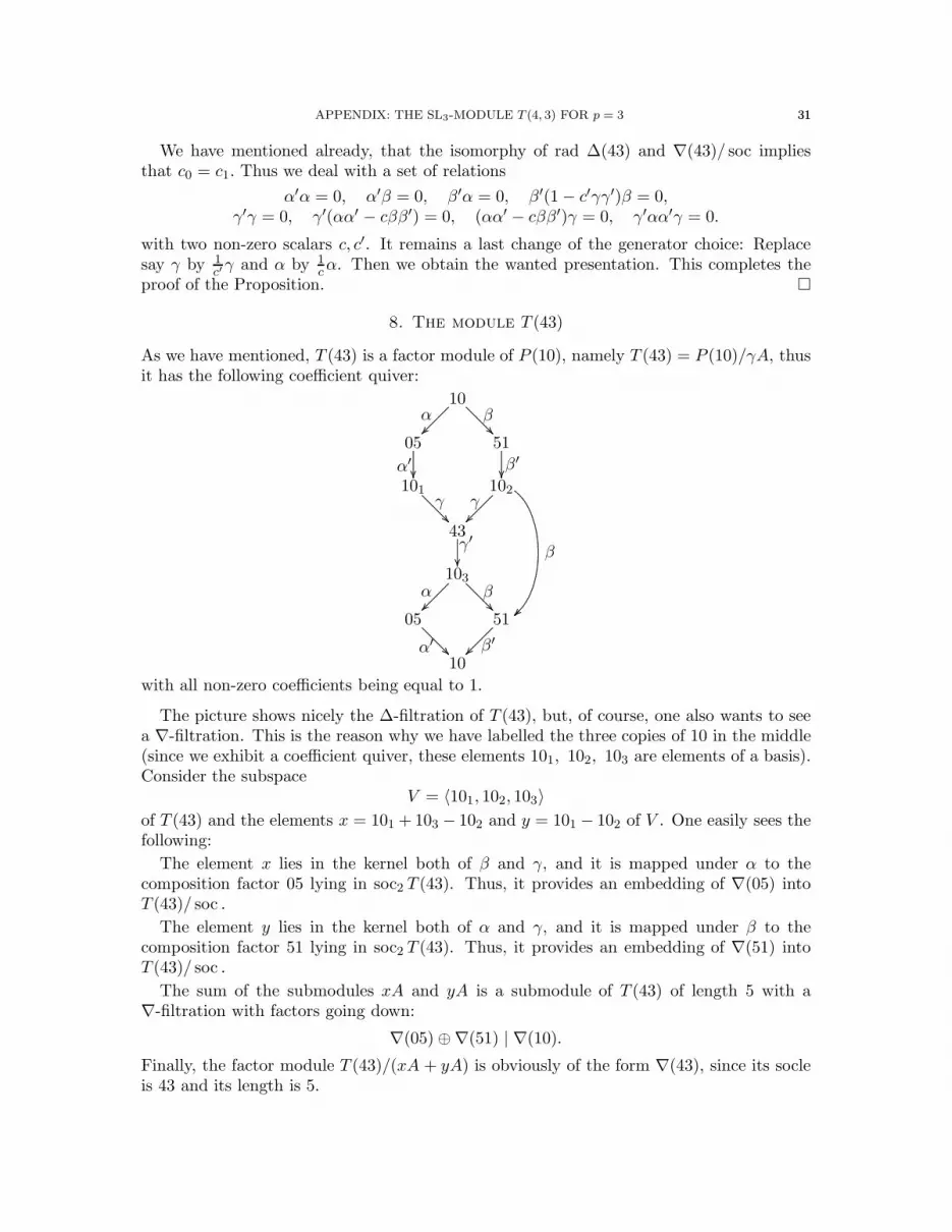
APPENDIX: THE SL3-MODULE T (4, 3) FOR p = 3 3131
We have mentioned already, that the isomorphy of rad ∆(43) and ∇(43)/ soc impliesthat c0 = c1. Thus we deal with a set of relations
α′α = 0, α′β = 0, β′α = 0, β′(1− c′γγ′)β = 0,γ′γ = 0, γ′(αα′ − cββ′) = 0, (αα′ − cββ′)γ = 0, γ′αα′γ = 0.
with two non-zero scalars c, c′. It remains a last change of the generator choice: Replacesay γ by 1
c′γ and α by 1
cα. Then we obtain the wanted presentation. This completes the
proof of the Proposition. �
8. The module T (43)
As we have mentioned, T (43) is a factor module of P (10), namely T (43) = P (10)/γA, thusit has the following coefficient quiver:
10
10
103
101 102
05
05
51
51
43
.........................................................................
..
.
.
.
.
.
.
.
.
.
.
.
........................................................................
............
.
........................................................................
.
..
.
.
.
.
.
.
.
.
.
.........................................................................
............
.
.
.
.
.
.
.
.
.
.
.
.
.
.
.
.
.
.
.
.
.
.
.
.
.
.
.
.
.
.
.
.
.
.
.
.
.
.
.
.
.
.
..
.
.
.
.
.
.
.
.
.
.
.
.
.
.
.
.
.
.
.
.
.
.
.
..
.......................................................................
.
.
.
..
.
.
.
.
.
.
.
.........................................................................
............
.........................................................................
..
.
.
.
.
.
.
.
.
.
.
.........................................................................
............
.
.
.
.
.
.
.
.
.
.
.
.
.
.
.
.
.
.
.
.
.
.
.
.
.
.
.
.
.
.
.
.
.
.
.
.
.
.
.
.
.
.
..
.
.
.
.
.
.
.
.
.
.
.
.
.
.
.
.
.
.
.
.
.
.
.
.
.
.
.
.
.
.
.
.
.
.
.
.
.
.
.
.
.
.
.
.
.
.
.
.
.
.
.
.
.
.
.
.
.
.
.
.
.
.
.
.
.
..
.
.
.
.
.
.
.
.
.
.
.
.
.
.
.
.
.
.
.
.
.
.
.
.............................................................................................................................................................................................................................
..
.....................
............
α
α
α′
α′
β
β
β
β′
β′
γ γ
γ′
with all non-zero coefficients being equal to 1.
The picture shows nicely the ∆-filtration of T (43), but, of course, one also wants to seea ∇-filtration. This is the reason why we have labelled the three copies of 10 in the middle(since we exhibit a coefficient quiver, these elements 101, 102, 103 are elements of a basis).Consider the subspace
V = 〈101, 102, 103〉
of T (43) and the elements x = 101 +103 − 102 and y = 101 − 102 of V . One easily sees thefollowing:
The element x lies in the kernel both of β and γ, and it is mapped under α to thecomposition factor 05 lying in soc2 T (43). Thus, it provides an embedding of ∇(05) intoT (43)/ soc .
The element y lies in the kernel both of α and γ, and it is mapped under β to thecomposition factor 51 lying in soc2 T (43). Thus, it provides an embedding of ∇(51) intoT (43)/ soc .
The sum of the submodules xA and yA is a submodule of T (43) of length 5 with a∇-filtration with factors going down:
∇(05)⊕∇(51) | ∇(10).
Finally, the factor module T (43)/(xA + yA) is obviously of the form ∇(43), since its socleis 43 and its length is 5.

3232 C.M. RINGEL
Remark. In terms of the basis of A presented above, we also can write:
x = αα′ + αα′γγ′ − ββ′
y = αα′ − ββ′.
9. A further look at the module T (43)
In order to understand the module T (43) better, let us concentrate on the essential partwhich looks quite strange, namely the three subfactors 101, 102, 103 shaded below:
10
10
101
102
103
05
05
51
51
43
.
........................................................................
.
..
.
.
.
.
.
.
.
.
.
..
.......................................................................
............
.........................................................................
.
.
..
.
.
.
.
.
.
.
.
.
........................................................................
............
.
.
.
.
.
.
.
.
.
.
.
.
.
.
.
.
.
.
.
.
.
.
.
.
.
.
.
.
.
.
.
.
.
.
.
.
.
.
.
.
.
.
..
.
.
.
.
.
.
.
.
.
..
.
.
.
.
.
.
.
.
.
.
..
.........................................................................
..
.
.
.
.
.
.
.
.
.
.
.
........................................................................
............
.
........................................................................
.
.
..
.
.
.
.
.
.
.
.
.........................................................................
............
.
.
.
.
.
.
.
.
.
.
.
.
.
.
.
.
.
.
.
.
.
.
.
.
.
.
.
.
.
.
.
.
.
.
.
.
.
.
.
.
.
.
..
.
.
.
.
.
.
.
.
.
.
.
.
.
.
.
.
.
.
.
.
.
.
.
.
.
.
.
.
.
.
.
.
.
.
.
.
.
.
.
.
.
.
.
.
.
.
.
.
.
.
.
.
.
.
.
.
.
.
.
.
.
.
.
.
.
..
.
.
.
.
.
.
.
.
.
.
.
.
.
.
.
.
.
.
.
.
.
.
.
.............................................................................................................................................................................................................................
.......................
............
α
α
α′
α′
β
β
β
β′
β′
γ γ
γ′
. . . . . . . . . . . . . . . . . . . . . . . . . . . . . . . . . . . . . . . .
. . . . . . . . . . . . . . . . . . . . . . . . . . . . . . . . . . . . . . .
. . . . . . . . . . . . . . . . . . . . . . . . . . . . . . . . . . . . . . . .
. . . . . . . . . . . . . . . . . . . . . . . . . . . . . . . . . . . . . . .
. . . . . . . . . . . . . . . . . . . . . . . . . . . . . . . . . . . . . . . .
. . . . . . . . . . . . . . . . . . . . . . . . . . . . . . . . . . . . . . .
. . . . . . . . . . . . . . . . . . . . . . . . . . . . . . . . . . . . . . . .
. . . . . . . . . . . . . . . . . . . . . . . . . . . . . . . . . . . . . . .
. . . . . . . . . . . . . . . . . . . . . . . . . . . . . . . . . . . . . . . .
. . . . . . . . . . . . . . . . . . . . . . . . . . . . . . . . . . . . . . .
. . . . . . . . . . . . . . . . . . . . . . . . . . . . . . . . . . . . . . . .
. . . . . . . . . . . . . . . . . . . . . . . . . . . . . . . . . . . . . . .
. . . . . . . . . . . . . . . . . . . . . . . . . . . . . . . . . . . . . . . .
. . . . . . . . . . . . . . . . . . . . . . . . . . . . . . . . . . . . . . .
. . . . . . . . . . . . . . . . . . . . . . . . . . . . . . . . . . . . . . . .
. . . . . . . . . . . . . . . . . . . . . . . . . . . . . . . . . . . . . . .
. . . . . . . . . . . . . . . . . . . . . . . . . . . . . . . . . . . . . . . .
. . . . . . . . . . . . . . . . . . . . . . . . . . . . . . . . . . . . . . .
. . . . . . . . . . . . . . . . . . . . . . . . . . . . . . . . . . . . . . . .
. . . . . . . . . . . . . . . . . . . . . . . . . . . . . . . . . . . . . . . .
. . . . . . . . . . . . . . . . . . . . . . . . . . . . . . . . . . . . . . .
. . . . . . . . . . . . . . . . . . . . . . . . . . . . . . . . . . . . . . . .
. . . . . . . . . . . . . . . . . . . . . . . . . . . . . . . . . . . . . . .
. . . . . . . . . . . . . . . . . . . . . . . . . . . . . . . . . . . . . . . .
. . . . . . . . . . . . . . . . . . . . . . . . . . . . . . . . . . . . . . .
. . . . . . . . . . . . . . . . . . . . . . . . . . . . . . . . . . . . . . . .
. . . . . . . . . . . . . . . . . . . . . . . . . . . . . . . . . . . . . . .
. . . . . . . . . . . . . . . . . . . . . . . . . . . . . . . . . . . . . . . .
. . . . . . . . . . . . . . . . . . . . . . . . . . . . . . . . . . . . . . .
. . . . . . . . . . . . . . . . . . . . . . . . . . . . . . . . . . . . . . . .
. . . . . . . . . . . . . . . . . . . . . . . . . . . . . . . . . . . . . . .
. . . . . . . . . . . . . . . . . . . . . . . . . . . . . . . . . . . . . . . .
. . . . . . . . . . . . . . . . . . . . . . . . . . . . . . . . . . . . . . .
. . . . . . . . . . . . . . . . . . . . . . . . . . . . . . . . . . . . . . . .
. . . . . . . . . . . . . . . . . . . . . . . . . . . . . . . . . . . . . . .
. . . . . . . . . . . . . . . . . . . . . . . . . . . . . . . . . . . . . . . .
. . . . . . . . . . . . . . . . . . . . . . . . . . . . . . . . . . . . . . .
. . . . . . . . . . . . . . . . . . . . . . . . . . . . . . . . . . . . . . . .
The three elements 101, 102 103 are displayed in two layers, namely in the radical layersthey belong to. If we consider the position of composition factors of the form 10 in the soclelayers, we get a dual configuration, since the subspace inside V generated by the difference101 − 103 lies in the kernel of γ and therefore belongs to soc3 T (43).
Let us look at the the space
V = 101 ⊕ 102 ⊕ 103,
in more detail, taking into account all the information stored there, namely the endomor-phism γ = γγ′ as well as the images of the maps to V and the kernels of the maps startingat V . One may be tempted to look at the subspaces
Im(α′), Im(β′), Ker(α), Ker(β),
however, one has to observe that the maps mentioned here are not intrinsically given, butcan be replaced by suitable others (as we have done when we were reducing the number ofparameters). For example, instead of looking at α′, we have to take into account the wholefamily of maps α′ + cα′γ with c ∈ k. Thus, the intrinsic subspaces to be considered are
U1 = Im(α′) + Im(α′γ) = Im(α′) + Im(γ),U2 = Im(β′) + Im(γ),U3 = Ker(α) ∩Kerγ,U4 = Ker(β) ∩Kerγ,
as well as Ker(γ) and Im(γ). However, since we see that
Ker(γ) = U3 + U4,Im(γ) = U1 ∩ U2,
it is sufficient to consider V with its subspaces U1, . . . , U4.
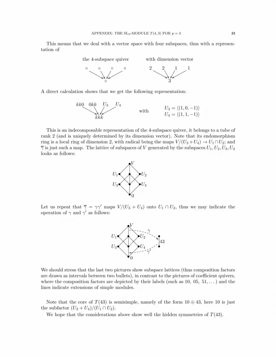
APPENDIX: THE SL3-MODULE T (4, 3) FOR p = 3 3333
This means that we deal with a vector space with four subspaces, thus with a represen-tation of
◦ ◦ ◦ ◦
◦
..................................................................................................................
.
.
.
.
.
.
.
.
.
..
.
.
.
.
.
.
.
.
.
.
.
.
.
.
.
.
.
.
.
..
.
.
.
.
.
.
.
.
.
.
.
.
.
.
.
.
..
.
..........
.
.
.
.
.
.
.
.
.
.
.
.
.
.
.
.
.
.
.
.
.
..
.
.
.
.
.
.
.
.
.
.
.
.
.
.
.
.
.
.
.
..
.
.
.
.
.
.
.
.
.
.
.
.
.
.
.
.
..
.
.
.
.
.
.
.
.
.
.
.
.
.
..........
......................................................................................................
............
the 4-subspace quiver
2 2 1 1
3
..................................................................................................................
.
.
.
.
.
.
.
.
.
.
..
.
.
.
.
.
.
.
.
.
.
.
.
.
.
.
.
.
.
.
..
.
.
.
.
.
.
.
.
.
.
.
.
.
.
.
..
..
.........
.
.
.
.
.
.
.
.
.
.
.
.
.
.
.
.
.
.
.
.
.
.
..
.
.
.
.
.
.
.
.
.
.
.
.
.
.
.
.
.
.
.
..
.
.
.
.
.
.
.
.
.
.
.
.
.
.
.
..
.
.
.
.
.
.
.
.
.
.
.
.
...........
......................................................................................................
............
with dimension vector
A direct calculation shows that we get the following representation:
kk0 0kk U3 U4
kkk
..................................................................................................................
.
.
.
.
.
..
.
.
.
.
.
.
.
.
.
.
.
.
.
.
.
.
.
.
.
..
.
.
.
.
.
.
.
.
.
.
.
.
.
.
.
.
.
.
.
....
..........
.
.
.
.
.
.
.
.
.
.
.
.
.
.
.
.
.
..
.
.
.
.
.
.
.
.
.
.
.
.
.
.
.
.
.
.
.
..
.
.
.
.
.
.
.
.
.
.
.
.
.
.
.
.
.
.
.
...
.
.
.
.
.
.
.
.
.
.
.
..
..........
......................................................................................................
............
withU3 = 〈(1, 0,−1)〉
U4 = 〈(1, 1,−1)〉
This is an indecomposable representation of the 4-subspace quiver, it belongs to a tube ofrank 2 (and is uniquely determined by its dimension vector). Note that its endomorphismring is a local ring of dimension 2, with radical being the maps V/(U3+U4) → U1∩U2; andγ is just such a map. The lattice of subspaces of V generated by the subspaces U1, U2, U3, U4
looks as follows:
•
•
•
•
• •
• •
.
.
.
.
.
.
.
.
.
.
.
.
.
.
.
.
.
.
.
.
.
.
.
.
.
.
.
.
.
.
.
.
.
.
.
.
.
.
.
.
.
.
.
.
.
.
.
.
.
.
.
.
.
.
.
.
.
.
.
.
.
.
.
.
.
.
.
.
.
.
.
.
.
.
.
.
.
.
.
.
.
.
.
.
.
.
.
.
.
.
.
.
.
.
.
.
.
.
.
.
.
.
.
.
.
.
.
.
.
.
.
.
.
.
.
.
.
.
.
.
.
.
.
.
.
.
.
.
.
.
.
.
.
.
.
.
.
.
.
.
.
.
.
.
.
.
.
.
.
.
.
.
.
.
.
.
.
.
.
.
.
.
.
.
.
.
.
.
.
.
..
...................................................................................................................................................................................................................................................................................................................................
.
................................................................................................................................................................................................................................................................................................................................... 0
V
U1 U2
U3 U4
Let us repeat that γ = γγ′ maps V/(U3 + U4) onto U1 ∩ U2, thus we may indicate theoperation of γ and γ′ as follows:
•
•
•
•
• •
• •
.
.
.
.
.
.
.
.
.
.
.
.
.
.
.
.
.
.
.
.
.
.
.
.
.
.
.
.
.
.
.
.
.
.
.
.
.
.
.
.
.
.
.
.
.
.
.
.
.
.
.
.
.
.
.
.
.
.
.
.
.
.
.
.
.
.
.
.
.
.
.
.
.
.
.
.
.
.
.
.
.
.
.
.
.
.
.
.
.
.
.
.
.
.
.
.
.
.
.
.
.
.
.
.
.
.
.
.
.
.
.
.
.
.
.
.
.
.
.
.
.
.
.
.
.
.
.
.
.
.
.
.
.
.
.
.
.
.
.
.
.
.
.
.
.
.
.
.
.
.
.
.
.
.
.
.
.
.
.
.
.
.
.
.
.
.
.
.
.
.
..
...................................................................................................................................................................................................................................................................................................................................
.
..
................................................................................................................................................................................................................................................................................................................................. 0
V
U1 U2
U3 U4 •
•
.
.
.
.
.
.
.
.
.
.
.
.
.
.
.
.
.
.
.
.
.
.
.
.
.
.
.
.
.
.
.
.
.
.
.
.
.
.
.
.
.
.
.
.
.
.
.
.
.
.
.
.
.
.
.
.
.
........ ........ ................
................
........
........
........
........
........
........
........ ........ ........
........................
........
........
........
........
........
........
....................
............
..................
............
γ
γ′
43
We should stress that the last two pictures show subspace lattices (thus composition factorsare drawn as intervals between two bullets), in contrast to the pictures of coefficient quivers,where the composition factors are depicted by their labels (such as 10, 05, 51, . . . ) and thelines indicate extensions of simple modules.
Note that the core of T (43) is semisimple, namely of the form 10 ⊕ 43, here 10 is justthe subfactor (U3 + U4)/(U1 ∩ U2).
We hope that the considerations above show well the hidden symmetries of T (43).

3434 C.M. RINGEL
Finally, let us remark that the module T (43) has a diagram D in the sense of Alperin(but no strong diagram), namely the following:
◦
◦
◦ ◦
◦
◦
◦
◦
◦
◦
.................................................
.
.
.
.
..
.
.
.
.
.
.
..
...............................................
............
.................................................
.
.
..
.
.
.
.
.
.
.
.
.................................................
............
.
.
.
.
.
.
.
.
.
.
.
.
.
.
.
.
.
.
.
.
.
.
.
.
.
..
.
.
.
.
.
.
.
.
.
.
.
.
.
.
.
.
.
.
.
.
.
.
.
.
................................................
..
.
.
.
.
.
.
.
.
.
.
..
...............................................
............
.................................................
.
..
.
.
.
.
.
.
.
.
.
.
................................................
............
.
.
.
.
.
.
.
.
.
.
.
.
.
.
.
.
.
.
.
.
.
.
.
.
.
..
.
.
.
.
.
.
.
.
..
.
.
.
.
.
.
.
.
.
.
..
.
.
.
.
.
.
.
.
.
.
.
.
.
.
.
.
.
.
.
.
.
.
.
.
.
.
..
.
.
.
.
.
.
.
.
..
.
.
.
.
.
.
.
.
.
.
..
.
(obtained from the coefficient quiver by deleting the by-path β).
10. A related algebra
We have used the ∆-filtration of T (43) in order to show that T (43) has simple socle, andthis implied that the coefficient cbb had to be non-zero. In this way, we have obtained thesomewhat strange relations presented in the Proposition. Let us now consider the samequiver Q(10, 05, 51, 43), but with the relations
α′α = 0, α′β = 0, β′α = 0, β′β = 0,γ′γ = 0, γ′(αα′ − ββ′) = 0, (αα′ − ββ′)γ = 0, γ′αα′γ = 0.
The corresponding algebra A′ still is quasi-hereditary, and the ∆-modules and the ∇-modules have the same shape as those for the algebra A = A(10, 05, 51, 43). However, nowit turns out that the tilting module for 43 is of length 11, with a ∆-filtration of the form
∆(10)⊕∆(10) | ∆(05) ⊕∆(51) | ∆(43)
and a similar ∇-filtration.
References
[ARS] M.Auslander, I.Reiten, S.Smalø: Representation Theory of Artin Algebras. CambridgeStudies in Advanced Mathematics 36, Cambridge University Press (1995).
[ASS] I.Assem, D.Simson, A.Skowronski: Elements of the Representation Theory of AssociativeAlgebras. 1. Techniques of Representation Theory. London Mathematical Society StudentTexts 65, Cambridge University Press (2007)
[BDM] C.Bowman, S.R.Doty, S.Martin: Decomposition of tensor products of modular irreduciblerepresentations for SL3.
[BR] R.A.Brualdi, H.J.Ryser: Combinatorial matrix theory. Encyclopedia of mathematics and itsapplications 39. Cambridge University Press. 1991.
[DD] M.De Visscher, S.Donkin: On projective and injective polynomial modules. Math. Z. 251(2005), 333-358.
[DR] V.Dlab, C.M.Ringel: The module theoretic approach to quasi-hereditary algebras. In:Representations of Algebras and Related Topics (ed. H.Tachikawa, S. Brenner). LondonMathematical Society Lectute Note Series 168. Cambridge University Press (1992).
[M] R.Martınez-Villa: Algebras stably equivalent to l-hereditary. In: Representation Theory II(ed. V.Dlab, P.Gabriel), Springer Lecture Notes in Mathematics 832 (1980), 396-431.
[R1] C.M.Ringel: Tame Algebras and Integral Quadratic Forms. Springer Lecture Notes inMathematics 1099 (1984)

APPENDIX: THE SL3-MODULE T (4, 3) FOR p = 3 3535
[R2] C.M.Ringel: The category of modules with good filtrations over a quasi-hereditary algebrahas almost split sequences. Math. Z. 208 (1991), 209-223.
[R3] C.M.Ringel: Exceptional modules are tree modules. Lin. Alg. Appl. 275-276 (1998) 471-493.[SS] I.Assem, D.Simson, A.Skowronski: Elements of the Representation Theory of Associative
Algebras. 2. Tubes and Concealed Algebras of Euclidean Type. London MathematicalSociety Student Texts 71, Cambridge University Press (2007)
CB: Corpus Christi College, Cambridge, CB2 1RH, England, UK
E-mail address: [email protected]
SRD: Mathematics and Statistics, Loyola University Chicago, Chicago, IL 60626, USA
E-mail address: [email protected]
SM: Magdalene College, Cambridge, CB3 0AG, England, UK
E-mail address: [email protected]
CMR: Fakultat fur Mathematik, Universitat Bielefeld, PO Box 100 131, D-33 501 Biele-
feld, Germany
E-mail address: [email protected]


