Embed Size (px)
Citation preview

1
DELIVERIES OPTIMIZATION BY EXPLOITING PRODUCTION TRACEABILITY INFORMATION
Simon TAMAYO, Thibaud MONTEIRO, Nathalie SAUER
LGIPM EA 3096 / INRIA - COSTEAM ENIM - Université Paul Verlaine - Metz
Île du Saulcy, 57012 METZ – Cedex, France [email protected], [email protected], [email protected]
ABSTRACT: The recent product traceability requirements, particularly in food production chains, demonstrate an industrial need to improve traceability systems. Having real-time access to traceability information allows its exploitation, which is the aim of this work. In this paper the problem of minimizing the cost of products recall is treated. First the raw material dispersion problem is analyzed, in order to determine a risk level criterion or “production criticality”. This criterion is used subsequently to optimize deliveries dispatch with the purpose of minimizing the number of batch recalls in case of crisis. This is achieved by implementing decision-making aid tools based on operational research and artificial intelligence.
KEYWORDS: Food traceability; Raw material dispersion; Genetic algorithms; Artificial neural networks; Expert systems; Optimization.
1. INTRODUCTION
Worldwide, recent legislation requirements have appeared concerning food traceability, which now must be established at all stages of production. Therefore traceability solutions have reached an important stage of development. This research is held within the project of designing a deliveries optimization unit, to be adapted to traceability software. The aim of this work is the reduction of the products recall cost, in case of a certain crisis by minimizing the quantity of products to be recalled. The presented work was carried out as a PhD research project in agreement with a software provider company working in the industrial traceability field.
The traceability system in the farming and food supply chain can be described as the documented identification of the operations which leads to the production and sale of a product (Bertolini et al., 2006). I.e. traceability refers to the capability to trace goods along the distribution chain on a batch number or series number basis. Traceability makes recalls possible, which contributes to food safety in the food industry, it links the information and material flow. The opportunity to connect traceability with the whole documentation and control system represents an effective means of boosting the consumer’s perception of food safety and quality (Moe, 1998).
The traceability information treatment assumes great quantity of data as well as an increasing information diversity, which can be translated as a need for computerization in addition to the implementation of some other functions like inventory control,
production planning, material output register and deliveries management. Computerized traceability solutions already exist, but as these solutions do not represent any kind of advantage to producers, they remain doing paper traceability, which is useless during a recall procedure. Although, traceability information can be used to improve the production and logistic fields, in order to obtain a supplementary benefit. (Wang et al., 2008) propose a MILP model (Mixed Integer Linear Programming) in order to optimize lot sizing for perishable food production. This optimization takes into account in the same analysis traceability and economic criteria.
In this paper, the main objective is to find a way of delivering in order to recall a minimum number of final products in case of crisis; this problems becomes complex in the case the raw materials cutting and assembling recipes optimization. The works around this matter have been deployed in relation with a software provider of the sector. Consequently a final product deliveries optimization is proposed using traceability information. Hence one not only traces the products in order to perform recalls possible, but also to achieve a better production and logistic management, reducing risk and cost in food recalls. That is to say, take into account the real production’s characteristics, given by the traceability information in order to assign the deliveries in a smarter way looking forward for a reduction of the recall size in case of crisis. A very important criterion to take into account is the “raw materials disperision” (wich will be formally presented in section 4).
The paper is organized as follows: after outlining the background and the problem statement, section 3
hal-0
0580
612,
ver
sion
1 -
28 M
ar 2
011
Author manuscript, published in "International Journal of Advanced Operations Management 1, 2/3 (2009) pp. 267 - 285" DOI : 10.1504/IJAOM.2009.030676

2
details the approach and shows the retained decision process. In section 4, the first step of our approach is detailed. After having defined the optimizing criterion (the raw materials dispersion in the final products), a model is proposed in order to solve it by a genetic algorithm. Then the production’s sanitary risk level (defined as criticality) is assigned for all production batches (section 5). This determination is made with a neural network which models the expertise of the logistic manager. In section 6, a solution to final product delivery optimization is proposed. This solution is compared with the FIFO strategy, generally used for delivery decision. Finally, conclusions and prospects are suggested in section 7.
2. PROBLEM STATEMENT
The risk impact and the ontological requirements of a traceability system have been studied in the past years (Borst et al., 1997). The relevance of product tracing in both the external supply chain and inside the production system has been considered by (Ramesh et al., 1997). The need for traceability computerization introduced previously has been studied by numerous authors like Sahin, Dallery and Gershwin (2002), who judge Information Technology to be the fundamental tool in the traceability of manufactured products. Several models of managing traceability information have been considered (Jansen-Vullers et al., 2003) as well as a general framework and a statement of experimental evidence (Regattieri et al., 2007) which have considered all the technological solutions in the traceability market.
Most of this scientific literature is focused on general factors such as identification technologies (tools and hardware solutions such as RFID, 2D Code, Processing board, etc.) and potential advantages. The problem of optimization in production was also considered from the traceability point of view, specifically regarding the raw material dispersion problem, to our knowledge this problem has first been formalized on the case of a sausage factory (Dupuy et al., 2005), the dispersion problem concept comes from this sausage manufacturing process. Pork meat industry is particularly interested in improving its traceability (Liddell and Bailey, 2001). In order to produce sausages, this company cuts pork meat in components like ham, belly, loin, trimmings… Further in the production process, these meat components are minced and mixed to create minced meat batches. These minced meat batches will be used to produce different types of sausages. Each type of raw material gives components in fixed proportions. This is the disassembling (or cutting) bill of material. A component can also come from different raw material types. The finished products (sausages) are composed of several components in given proportions. This is the assembling (or mixing)
bill of material. During a working day, the company receives several batches of different types of raw material (ham, side of pork, shoulder…). So, many batches of components will be created and also many finished product batches. The purpose of the company is to minimize the cost due to a food safety crisis. If the food safety problem comes from a raw material batch, the company will identify (tracing) and recall all products which contain the raw material. If it concerns a finished product, the company will identify (tracking) the raw material batches and then recall all the corresponding finished products. So, in order to minimize the cost of a food safety crisis, the company has to minimize the number of recalled products. In the case of sausage production, batch size should be reduced but also batch mixing. The more raw material batches are mixed in finished product batches, the more important the recall and the cost.
Dupuy’s works (2004) finally leads us to the purpose of this paper which does take advantage of traceability information in order to obtain a benefit in other fields of production and management.
In order to achieve this aim, this paper presents a methodological approach to the problem, starting with an activity analysis which enables the definition of the main work axis. Thus, three principal subjects are defined as follows: dispersion evaluation and optimization, criticality determination and final product delivery optimization. As a matter of fact, this approach allows the producer to identify the failures on its production recipe, the most critical elements within its production chain, and therefore improve the performance of delivery allocation. Moreover, this final optimization can be measured as a reasonable decrease in the recall size, hence a significant economic stake.
To achieve the final purpose of reducing the recall size and cost one must perform an intelligent delivery allocation. Therefore, this supposes a previous knowledge of the production in terms of “recall risk”, which depends on several production factors, chiefly on the raw material dispersion. Consequently, this dispersion value needs to be modelled and optimized. To that end, the initial section consists of raw material dispersion optimization, a criterion used subsequently for the determination of the criticality index of production batches. From which we get to finally develop an optimization of the manufacturing product delivery in order to reduce the number of batch recalls in case of a crisis.
3. GLOBAL APPROACH
This paper focuses on the integration of several manufacturing parameters into a raw material dispersion diagnosis, inside the internal production chain. Thus, it aims at optimizing packing and
hal-0
0580
612,
ver
sion
1 -
28 M
ar 2
011

3
distribution criteria, considering possible critical situations. It is imperative to know the “risk” to send a potentially perilous production to an important customer, or to the big distribution market (which supposes a dispersion increase over the external chain). Therefore, one would like to assign in an optimal way the production outgoing batches to the delivery orders.
Globally, the traceability information regarding the initial product cutting and mixing leads to a dispersion evaluation and optimization of the fabrication recipe. Therefore, this dispersion and some other traceability indicators are computed to obtain a criticality value of the production. Lastly, this criticality allows an optimization of the delivery order allocation. In the SADT activity diagram (Marca et al., 2006), shown in Figure 1, a logical order to solve the earlier mentioned problems is exposed, according to the sequence of information. The need to find solutions to evaluate dispersion should be noted because these dispersion values will be fundamental for production criticality determination and thus the ulterior delivery assignment.
4. DISPERSION OPTIMIZATION
The developed tool is presented to face the dispersion optimization problem. In the methodology summarised in the Figure 1, a genetic algoritm has been selected for the resolution of the mentioned problem. It is shown that the optimization of the raw material input allocation towards the fabrication products is NP–hard; this is why a meta-heuristic method is selected for its resolution.
4.1. Definition of dispersion (Dupuy et al., 2002)
The descending dispersion of a raw material batch is the number of batches of finished products which contain a part of this raw material. The ascending dispersion of a finished product batch is the number of raw material batches used in this finished product. The total dispersion of a system, as is shown in Figure 2, is equal to the summation of the descending dispersions of all raw material batches and the ascending dispersions of all finished products.
To decrease this dispersion, we must determine the way of distributing raw materials throughout production, as well as the way of assembling finished products from sub-products in a multistage production configuration.
4.2. Problem’s complexity
(Dupuy et al., 2005) proposed a mathematical model based on MILP programming to optimize dispersion in food industry. Optimization is made with LINGO 6.0 software. This approach can only be used for small problems. With real industrial problems, computing time using deterministic algorithms widely increases.
Main serverDeliveriesTerminal
Dispersion evaluation of the
production batches
Criticality determination for
the production batches
Deliveries assignment
(batches – orders)
PlanningInformation
DispersionValues
CriticityValues
MILP modelGA
ArtificialNeural Network
ChoiceBatch-DO
History And markers
SanitaryStandards
DispersionValues
DO’s Clients Information
Traceability Information
ExpertSystem
InformationSuppliersAnd conveyors
SanitaryAlarms
Figure 1. Main activities diagram decomposition
Figure 2. Example of total ascending and descending dispersion
== 44
33
TToottaall DDiissppeerrssiioonn == 77
DDeesscceennddiinngg DDiissppeerrssiioonn == 44
aanndd
AAsscceennddiinngg DDiissppeerrssiioonn == 33
hal-0
0580
612,
ver
sion
1 -
28 M
ar 2
011

4
Indeed, we prove that this decision problem belongs to the NP-complete problems (see Theorem 1). A calculation of complexity shows that the total number of possible combinations C is:
∑=
=
=
=
∗=
RMBj
j
Qi
i
njiQEC
10,
max)( (1)
Where: C: Number combinations to calculate. E: Number of production levels. Qmax: Maximum quantity allowed by the recipe. Qi.j: Quantity of raw materials to allocate (integer). BRM: Number of raw material batches. n: Quantity of products to fabricate. i: Raw materil index. j: Product index.
Theorem 1. The dispersion optimization is NP-hard.
Proof. We prove the hardness of the dispersion optimization by showing that its decision version has the same form as the one from the “graph coloring problem”. In fact, the total number of possible combinations for the dispersion optimizing problem, given by formula (1), is the same as the “graphs coloring problem” (Wegener, 2005). As the latter problem is NP-hard, it allows concluding that the complexity of the dispersion optimizing problem is NP-hard.
With a NP-complete problem, the existence of a solution algorithm of polynomial complexity remains unknown (Palekar et al., 1990). As a result, when the problem size is important and the response time requierements are limited, meta-heuristic methods are considered. A genetic algorithm is presented in the following section.
4.3. The genetic algorithm (GA)
Genetic algorithms belong to a class of stochastic search methods that work iteratively on a population of candidate solutions to the problem (individuals), performing a search guided by the “fitness” (i.e. the value of the objective function) of each solution (Holland, 1975) and (Goldberg, 1994). In particular, the higher the fitness, the more the genes of a solution are likely to be propagated to the next iterations (Naso et al., 2007). This Darwinian principle is emulated with specific crossover, mutation and selection operators, which are applied with stochastic mechanisms that make the GA explore solutions with increasing fitness. Thus, their flexibility is geared towards the characteristics of the
objective function; the GA fits perfectly to the dispersion optimizing problem, as they do not rely on specific a priori hypotheses (e.g. continuity and convexity).
In the following section, the different stages of GA are presented according to this plan:
• Initial population
• Evaluation
• Selection
• Crossing
• Mutation
• Parameters setting
4.3.1. Initial population creation
The algorithm starts with numerous alternative solutions to the optimization problem, which are considered individuals in a population. In order to create a population adapted to our raw-material distribution problem, a function was developed, defining the problem’s initial conditions, that is to say, the configuration and characteristics of the production to be optimized. Thereafter, random matrices, called participation matrices, were created, containing the assignment allocations of raw-materials vs. fabrication products (Figure 3A). A matrix is created each time products are cut or composed, i.e. for each choice of outgoing material. There will be as many solution matrices as production stages minus one. These solutions are arbitrarily created, using random generating tools in an orderly manner, this trying to ensure coverage of all space solutions.
001100RM4
101011RM3
001110RM2
100101RM1
SP6SP5SP4SP3SP2SP1
001100RM4
101011RM3
001110RM2
100101RM1
SP6SP5SP4SP3SP2SP1
00Q44Q4300RM4
Q360Q340Q32Q31RM3
00Q24Q23Q220RM2
Q1600Q130Q11RM1
SP6SP5SP4SP3SP2SP1
00Q44Q4300RM4
Q360Q340Q32Q31RM3
00Q24Q23Q220RM2
Q1600Q130Q11RM1
SP6SP5SP4SP3SP2SP1
A) Participation matrix (raw materials - sub products)
B) Quantities assignment (raw materials - sub products)
Figure 3. Participation and quantites assignment matrices
hal-0
0580
612,
ver
sion
1 -
28 M
ar 2
011

5
4.3.2. Evaluation
Once the population is created, its behavior must be evaluated. Thus, one must count each individual’s total dispersion value which corresponds to its fitness. Afterwards a classification of the population is performed. For every individual, one determines the adaptation value which is conversely proportional to its classification. According to each individual’s adaptation a number of reproductions is assigned (for the next generation). The more the adaptation value is important, the more the individual is used for the reproduction. Therefore every individual has an adaptation value, a dispersion value and a number of reproductions for the next generation.
4.3.3. Selection and elitism
Before making the population’s “natural selection” by fitness, the best individuals of the preceding generation are added to the next generation, which enable the GA not to lose the best solutions through the evolution. Therefore, the best individuals of this hybrid generation are stored in a new generation list. This elitism is necessary for the convergence of the method. The size of the elite selection can variate as a parameter depending on the problem. An example of those selection rules and meta-heuristics can be found in (Siarry and Michalewicz, 2007) and (Talbi, 2006).
4.3.4. Crossing
To carry out the reproduction of the population’s individuals, random reproduction couples are assigned, while respecting the numbers of reproductions indicated in the evaluation. Once the list of couples is established, each one is taken (father and mother) to create an individual child who inherits from each of its parents half of the solution (as shown in Figure 4). This is carried out in order to be able to respect nomenclature constraints automatically, without needing to correct the children’s composition after each reproduction. So, this crossing solution is chosen to gain computational time. Other crossing operators could be used to gain efficiency (Holger and Stützle, 2004) and (Talbi, 1999), but require to repair new children.
4.3.5. Mutation
To mutate the individuals of a generation, the procedure used consists in performing random changes in the quantities distribution of each individual (the result of these changes can be degradation in terms of dispersion).
After the initial matrix composition, the coherence between the solution’s parts is verified. If in a stage of production, raw material is assigned to a product, then the solution of the following stage must respect this constraint. If it is not in case, an adaptation step has to be used.
Thereafter, random quantities are assigned while observing the problem’s limiting conditions by the quantities and the nomenclatures defined previously. As a result, a group of matrices, called assignment matrices, is obtained; each one contains the raw material distribution for all production stages, indicating for each option of assignment, the quantity to be sent, or zero, if the choice of assignment is not made (Figure 3B). If the arising problem contains sub-products coming from external suppliers (which are not manufactured from the materials contained in the preceding production stage), parallel participation and assignment matrices are created. Finally all the quantities assignment matrices toghether correspond to an individual of the population.
00Q144Q14300RM4
Q1360Q1340Q132Q131RM3
00Q124Q123Q1220RM2
Q11600Q1130Q111RM1
SP6SP5SP4SP3SP2SP1
00Q144Q14300RM4
Q1360Q1340Q132Q131RM3
00Q124Q123Q1220RM2
Q11600Q1130Q111RM1
SP6SP5SP4SP3SP2SP1
Father
Q246Q245000Q241RM4
000Q2330Q231RM3
Q226Q225Q2240Q2220RM2
Q216Q2150Q2130Q211RM1
SP6SP5SP4SP3SP2SP1
Q246Q245000Q241RM4
000Q2330Q231RM3
Q226Q225Q2240Q2220RM2
Q216Q2150Q2130Q211RM1
SP6SP5SP4SP3SP2SP1
Mother
Q246Q2450Q14300RM4
0000Q132Q131RM3
Q226Q225Q224Q123Q1220RM2
Q216Q2150Q1130Q111RM1
SP6SP5SP4SP3SP2SP1
Q246Q2450Q14300RM4
0000Q132Q131RM3
Q226Q225Q224Q123Q1220RM2
Q216Q2150Q1130Q111RM1
SP6SP5SP4SP3SP2SP1
New individual
Figure 4. Child creation
hal-0
0580
612,
ver
sion
1 -
28 M
ar 2
011
6
00Q144Q1
4300RM4
Q1360Q1
340Q132Q1
31RM3
00Q124Q1
23Q10RM2
Q11600Q1
130Q111RM1
SP6SP5SP4SP3SP2SP1
00Q144Q1
4300RM4
Q1360Q1
340Q132Q1
31RM3
00Q124Q1
23Q10RM2
Q11600Q1
130Q111RM1
SP6SP5SP4SP3SP2SP1
1st production level
Q24600Q2
4300FP4
Q23600Q2
330Q231FP3
00Q2240Q2
220FP2
00Q214000FP1
SP6SP5SP4SP3SP2SP1
Q24600Q2
4300FP4
Q23600Q2
330Q231FP3
00Q2240Q2
220FP2
00Q214000FP1
SP6SP5SP4SP3SP2SP1
2nd production level
00Q144Q1
4300RM4
Q1360Q1
340Q132Q1
31RM3
00Q124Q1
23Q10RM2
Q1160000Qm1
11RM1
SP6SP5SP4SP3SP2SP1
00Q144Q1
4300RM4
Q1360Q1
340Q132Q1
31RM3
00Q124Q1
23Q10RM2
Q1160000Qm1
11RM1
SP6SP5SP4SP3SP2SP1
1st production level after mutation
Qm246000Qm2
420FP4
Qm23600Qm2
330Qm231FP3
00Q224000FP2
00Q21400Qm2
11FP1
SP6SP5SP4SP3SP2SP1
Qm246000Qm2
420FP4
Qm23600Qm2
330Qm231FP3
00Q224000FP2
00Q21400Qm2
11FP1
SP6SP5SP4SP3SP2SP1
2nd production level after mutation
Figure 5. Mutation example
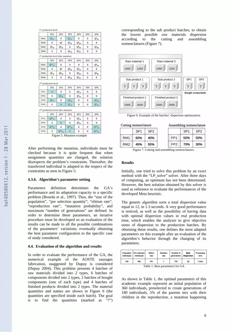
After performing the mutation, individuals must be checked because it is quite frequent that when assignment quantities are changed, the solution disrespects the problem’s constraints. Thereafter, the transferred individual is adapted to the respect of the constraints as seen in Figure 5.
4.3.6. Algorithm’s parameter setting
Parameters definition determines the GA’s performance and its adaptation capacity to a specific problem (Bourda et al., 1997). Thus, the “size of the population”, “pre selection quantity”, “elitism rate”, “reproduction rate”, “mutation probability”, and maximum “number of generations” are defined. In order to determine these parameters, an iterative procedure must be developed so an evaluation of the results can be made to all the possible combinations of the parameters’ variations; eventually obtaining the best parameter configuration to the specific case of study considered.
4.4. Evaluation of the algorithm and results
In order to evaluate the performance of the GA, the numerical example of the AOSTE sausages fabrication, ssuggested by Dupuy is considered (Dupuy 2004). This problem presents 4 batches of raw materials divided into 2 types, 6 batches of components divided into 2 types, 2 batches of bought components (one of each type) and 4 batches of finished products divided into 2 types. The material quantities and names are shown in Figure 6 (the quantities are specified inside each batch). The goal is to find the quantities (marked as “?”)
corresponding to the sub product batches, to obtain the lowest possible raw materials dispersion according to the cutting and assembling nomenclatures (Figure 7).
Raw material 1
1000
Raw material 2
Sub product 1
? ? ?
Sub product 2
? ? ?
1200 1000 1200
Finished product 1
2000
Finished product 2
2000 2000 2000
SP1
?Bought components
SP2
?
Raw material 1
1000
Raw material 2
Sub product 1
? ? ?
Sub product 2
? ? ?
1200 1000 1200
Finished product 1
2000
Finished product 2
2000 2000 2000
SP1
?Bought components
SP2
?
Figure 6. Example of the batches’ dispersion optimization
55%45%RM2
40%60%RM1
SP2SP1
30%70%FP2
50%50%FP1
SP2SP1
Cutting nomenclature Assembling nomenclature
55%45%RM2
40%60%RM1
SP2SP1
55%45%RM2
40%60%RM1
SP2SP1
30%70%FP2
50%50%FP1
SP2SP1
30%70%FP2
50%50%FP1
SP2SP1
Cutting nomenclature Assembling nomenclature
Figure 7. Cutting and assembling nomenclatures.
Results
Initially, one tried to solve this problem by an exact method with the “LP_solve” solver. After three days of computing, an optimum has not been determined. However, the best solution obtained by this solver is used as reference to evaluate the performances of the developed Meta heuristic.
The genetic algorithm sorts a total dispersion value equal to 12, in 1.3 seconds. A very good performance is noticed, as well as the possibility of having data with optimal dispersion values in real production time, which enables the analyzer to give objective notes of dispersion to the production batches. By obtaining these results, one defines the most adapted parameters on this example after an evaluation of the algorithm’s behavior through the changing of its parameters.
180
Population Individuals
1.3sec1270015%360
Processingtime
Best Dispersion
Number ofgenerations
Mutationrate
Elitism rate
Pre selection individuals
180
Population Individuals
1.3sec1270015%360
Processingtime
Best Dispersion
Number ofgenerations
Mutationrate
Elitism rate
Pre selection individuals
Table 1. Best parameters for GA
As shown in Table 1, the optimal parameters of this academic example represent an initial population of 360 individuals, preselected to create generations of 180 individuals, 5% of the parents mix with their children in the reproduction, a mutation happening
hal-0
0580
612,
ver
sion
1 -
28 M
ar 2
011

7
each generation and a maximum number of 700 generations.
Figure 8 illustrates the solution given by the GA, containing the dispersion value and the quantity assignment for the allocations of “raw materials vs. sub-products”, of “sub-products vs. finished products” and of “bought sub-products vs. finished products”.
A fast convergence into a very acceptable solution is noticed. In this convergence graph (Figure 9) the evolution of the population towards the optimum is shown, as well as the disturbances caused by the mutations, which frequently exit the solutions from local optimums, allowing the population to reach the global optimum easily.
It is possible to have very fast convergence due to the fact that the population procreates a “great individual”. This one being too often chosen, the
population tends to converge on its genome. In that specific case “the diversity of the genetic pool is then too reduced so that AG can progress” (Rennard, 2006).
5. CRITICALITY DETERMINATION
In the activities decomposition presented at the beginning, the use of an artificial neural network was considered in order to determine criticality associated to production. Neural networks are non-linear statistical data modeling tools which can be used to model complex relationships between inputs and outputs or to find patterns in data (Rich et al., 1990).
5.1. Definition of criticality
In this application “criticality” is defined as an index associated to production or to a batch of production which represents quantitatively its state of current risk. Criticality makes it possible to take into account simultaneously several parameters of manufacture in only one value exposing the potential danger. The goal is to obtain coherent criticality values by exploiting traceability information. Therefore, it is a question of making a multi-criteria decision and of assigning a criticality value to a list of entries as shown in Figure 10
Production markers
Traceability Information
Criticalitydetermination
Criticality value BatchProduction markersProduction markers
Traceability Information
Criticalitydetermination
Criticality value BatchBatch
Figure 10. Criticality determination statement.
This application seeks to develop an artificial neural network that allows producers to consider all possible types of indicators. Indeed, neural network models can be used to infer a function from observations even if the complexity of the data or task makes formal design of such a function difficult (Najafi et al., 1998), (Yu et al., 2005). To determine the criticality value, much traceability information has to be taken into account. This information could be qualitative (example: quality of suppliers) and quantitative (example: dispersion note). The
1110249010605504801140720450Tot SPj
5901110001002900520138008000020
00530470057004300053004705704300
10605504801140720450Tot SPj
660005400005500004500048007200
4000060000RM's > SP's
SP's > FP's ExtSP's > FP's
1110249010605504801140720450Tot SPj
5901110001002900520138008000020
00530470057004300053004705704300
10605504801140720450Tot SPj
660005400005500004500048007200
4000060000RM's > SP's
SP's > FP's ExtSP's > FP's
RM 1
1000
RM 2
SP1
450 1140
SP 2
1200 1000 1200
FP 1
2000
FP 2
2000 2000 2000
SP 1
Bought components
SP 2
720 480 1060550 2490 1110
RM 1
1000
RM 2
SP1
450 1140
SP 2
1200 1000 1200
FP 1
2000
FP 2
2000 2000 2000
SP 1
Bought components
SP 2
720 480 1060550 2490 1110
Figure 8. Solution to the evaluation example dispersion = 12,
time = 1.35.6 sec
Number of generations
Tota
l Dis
pers
ion
Number of generations
Tota
l Dis
pers
ion
Figure 9. Minimal dispersion and mean dispersion for 1000 generations.
hal-0
0580
612,
ver
sion
1 -
28 M
ar 2
011

8
criticality value depends on the industrial context and has to be adapted to each situation. So it is difficult to make a formal design of criticality function.
Nevertheless, a production process expert can give an evaluation of this criticality value without being able to formalize the inference process. Neural networks, as systems capable of learning, operate the principle of “induction”, i.e. acquiring training by experiencing. So, they are fully successful to solve the determination problem of the criticality value. Furthermore, this determination is a statistical problem of filter type with possibly noisy data input. It is a problem for which the neural networks have shown their effectiveness (Shin et al., 1992) and (Martin and Howard, 1996).
The problem was solved by using a neural network of the linear filter type and by a supervised training of it. The developed tool can be exploited in several fields. Once the network is designed, a simple reset and training will enable it to be exploited in a different field of production with other incoming parameters.
5.2. Creation of a training database
Before using the artificial neural network, a training database containing the list of examples must be formalized. The parameters establishing the production criticality must be defined initially. The following criteria were considered (Figure 11):
Criticality4775110
Output
Remaining days1052015300
Production stops020103
Suppliers note9135101
Dispersion note61025101
Inputs
Criticality4775110
Output
Remaining days1052015300
Production stops020103
Suppliers note9135101
Dispersion note61025101
Inputs
Figure 11. Artificial neural network’s Inputs and Outputs example.
• A dispersion note coming from the previously developed module; this note represents the ratio between the production’s real dispersion and the optimal dispersion that the production could have had. It varies from 1 to 10 (1 being a bad dispersion and 10 an optimal dispersion).
• A general supplier’s note, including raw material suppliers and dry material suppliers (plastic and paper). It is an average note of the suppliers group associated to the current production. It varies from 1 to 10, 1 being the equivalent to very bad suppliers and 10 to the optimal suppliers. In the food industry there is a real presence high and low quality suppliers,
manufacturers must adapt their production to the demand forecasts with the available raw materials which means in certain cases, the use of low quality raw materials.
• The number of production stops. This value varies from 0 to 3, 0 being a production without stops (optimal lifecycle in the production) and 3 being the maximum possible stops. Hence, an increase in production time and a lifecycle less appropriate. It is important to consider the number of stops in production because the life cycle of food products is particularly sensitive to changes in state and temperature. For example, frozen meat must remain on the machines blenders a specific time, and a production stop during the mixing process can represent a significant change in the BBD (best before date) or in the product’s sanitary risk level.
• Response Number of remaining days. This value takes into account the expiration date of the raw materials while assigning the nearest expiration date of the raw materials involved to the finished products. This value varies from 0 to 30 days, 0 being a catastrophic value, and 30 days an optimal value).
Considering the presented criteria, a set of examples was manually generated by means of an expert in the food production domain.
5.3. Creation of the artificial neural network
The programming strategy is supported by MATLAB’s “Neural Network Toolbox”. The program initially loads all the training examples, which can be constantly modified or enriched. The construction procedure starts by assigning the initial weights and biases of the network. First, all the weights and biases are set to zero. Then the network is modified according to the loaded examples by adapting the weights and biases to them. In order to ensure an optimal effectiveness, the training is carried out. A number of training iterations is limited in order to have a stop criterion. Subsequently, the network is trained until it is ready to make its own criticality decisions. However, if it needs to be adapted to special evaluation situations, it would have to receive extra training, considering new inputs.
5.4. Evaluation of the artificial neural network
To evaluate the application, a network was generated and then a simulation of its behavior was carried out by entering a set of random inputs and by watching the criticity output, after having rounded up this value to the nearest integer.
hal-0
0580
612,
ver
sion
1 -
28 M
ar 2
011

9
5.5. Results
Table 2 shows the criticity results for a random set of input parameter values.
519337
428138
5122104
619055
2243108
80345
91218
417178
611076
523235
610256
430053
620129
60089
671102
CriticalityDays leftProduction stops
Suppliers note
Dispersion note
519337
428138
5122104
619055
2243108
80345
91218
417178
611076
523235
610256
430053
620129
60089
671102
CriticalityDays leftProduction stops
Suppliers note
Dispersion note
Table 2. ANN evaluation results
These results were reasonable. The artificial neural network developed gives a very logical set of results containing criticity values, which could be exploited as production re-engineering criteria. These results confirm the good choice of the type of network and open new horizons to continue the development towards future optimizations.
6. FINAL PRODUCTS DELIVERIES OPTIMIZATION
The aim of this final section is to reduce potential product recall costs. The risks of recall vary significantly. Therefore, it is important to consider the necessary indicators, in order to properly diagnose and assign the production of outgoing batches to the delivery orders. The last part of the work presents real-time decisions and actions, which stand for the benefit to be obtained from information that has been collected and analyzed.
Actual deliveries priority criteria and constraints must be considered. The most representative criteria are summarized in Table 3
FIFO Criterion (first in – first out). 6
Maximum reception date (given by the client).5
Carrier.4
Client type.3
Distance from the client.2
Batch quantity (Number of batches Requested in the delivery order).1
CriterionPriority
FIFO Criterion (first in – first out). 6
Maximum reception date (given by the client).5
Carrier.4
Client type.3
Distance from the client.2
Batch quantity (Number of batches Requested in the delivery order).1
CriterionPriority
Table 3. Assignment choice criteria for the production batches
deliveries.
The tool to be developed must be able to operate as an expert, while making delivery choices after reasoning facts and known criteria. This is why using an expert system seems to be the best choice for this task.
Expert systems aim at exploiting the specialized skills or information on specific areas. They are used for diagnostic problems from experience (Buchanan and Shorttiffe, 1984) which is the main purpose in the deliveries cohice optimizationp roblem. Expert systemps can also be used as information guidance systems for planning and scheduling (Ajith, 2003), the type of application that one seeks to develop. This kind of system can analyze a set of one or more potentially complex and interacting goals in order to determine a set of actions to achieve those goals and/or provide a detailed temporal ordering of those actions, taking into account personnel, material, and other constraints (Feigenbaum et al., 1995). The presented tool will be able to plan the deliveries as it acquires the corresponding knowledge. Hence, knowledge acquisition is the most important element in the development of an expert system (Niwa et al., 1988).
The application’s main code invokes a function which recovers the matrix containing the set of manufacturing batches with their criticality values, as well as a matrix containing the set of delivery orders (and their implicit information, delivery date, client, carrier…). After the evaluation of the dispatch rules and priorities, the assignation choice is made.
The expert system is composed of a set of rules that analyze information (usually supplied by the user of the system) about a specific class of problems, as well as providing a certain analysis of the problem and recommending a set of actions or decisions (Mariot et al., 1989). In the case of deliveries optimization, the expert system must receive the set of delivery orders and outgoing batches, then, according to the priority criteria/constraints and the criticity values, assign in the best possible way to the outgoing allocations as shown in Figure 12.
Batch
Expert System
Delivery Order (DO) Choice
BatchBatch
Expert System
Delivery Order (DO)Delivery
Order (DO) Choice
Figure 12. Inputs and outputs for the expert system
6.1. Rules database
The criticity values are contained between 1 and 10. We started to write the assignation rules considering the variation of these criticity entries starting with the destination choice for the most critical batches and
hal-0
0580
612,
ver
sion
1 -
28 M
ar 2
011

10
finishing by the batches which represent less risk. An example of implemented rules database is presented in Table 4.
6.2. System’s inference engine
The decision execution starts by counting the quantity of batches presenting the same criticity value. Then, for each rule, the engine seeks the delivery order to be affected (regarding the characteristics mentioned in Table 3), and starts to assign the batches there, taking into consideration the orders already satisfied and the priority parameters. In the case of an homogeneus production and a short set of DO’s, the process can be simply algorithmic, but whenever the criticality values start to variate, as well as the clients, the assignment choice depends on several parameters wich may not be related at all. As an example, the DO’s shown in Table 5 are assigned in Figure 13.
The assignment choice given by the expert system is a matrix, which contains for each batch the number of the delivery order that will be associated to it. Moreover, the system sends the most critical batches
towards additional sanitary tests. Therefore, the “blocked batches” will be missing in one of the orders (assuming that we have the same number of batches to manufacture as batches ordered to dispatch) until obtaining the test results.
6.3. Evaluation of the expert system vs. FIFO allocation
In order to evaluate the performance of the obtained results, it is important to compare them with a typical FIFO delivery assignment (the most used method in the food industry). In order to do this, a quantity of manufacturing batches was considered as well as a set of delivery orders. Then, the dispatch choice was made twice: first with the expert system (considering the value of criticity given by the artificial neural network) and second using the FIFO criterion (without considering criticity). As a result, two different lists of assignment were sorted in order to be evaluated. Subsequently, several crisis cases were simulated. Thereafter, the quantity of recalled batches was counted for each method and then these values were compared (FIFO recalls vs. Expert System recalls). With the purpose of considering a wide range of cases, this procedure was done for different batch quantities of 1 000, 2 000 and 3 000 that were distributed between 8, 12, or 20 delivery orders with randomly determined requested quantities and with crisis probabilities of 0.05%, 0.10% and 0.15% proportional to the production’s criticity values.
Table 6 shows the results of this evaluation, which was carried out with a Monte Carlo simulation. For each different configuration of # of batches, # of DO’s and crisis probability, the number of recalled batches is presented for the expeditions choices by FIFO and ES, in each case the pourcentage of benefit obtained by the ES is shown. The obtained results are very satisfactory indeed. It is evident, there is a significant improvement in the distribution is made by the expert system in terms of recalled batches.
Figure 14 illustrates the difference between the recalls in case of crisis according to the two used
……
Fill the orders with these products (as they come from a low risk batch, there is no
harm in “spreading” them)THEN
The batches have a criticality of 1 and there are products missing in
the DO’sIF
Send all the products of this batch togetherTHENThe batch have a criticality of 9
and there is a DO with a quantity that can held all batch
IF
Make extra sanitary tests to this batch’s productsTHEN
The batch have a criticality of 10 and the DO comes from a small
clientIF
Table 4. Example of batch deliveries rules
2333046
1212465
3133094
3312953
3315022
3333441
Date Note
Carrier Type
Client TypeQuantity# DO
2333046
1212465
3133094
3312953
3315022
3333441
Date Note
Carrier Type
Client TypeQuantity# DO
Table 5. Example of DO set.
# B
atch
es
# DO’s
# B
atch
es
# DO’s Figure 13. Assignment choice of deliveries for a set of
Batches and DO’s
Num
bero
f rec
alls
Iterations
Num
bero
f rec
alls
Iterations Figure 14. Batches pointed out for the two different assignment
criteria, for 50 iterations. (2000 production batches for 8 delivery orders with a crisis probability of 0.15%).
hal-0
0580
612,
ver
sion
1 -
28 M
ar 2
011

11
criteria. The surface formed by the recalls of the expert system is considerably less important than that of the FIFO. Particularly where the recall is really dramatic, the considerable impact of implementing this decision-making aid tool is clearly identifiable.
In the case illustrated in Figure 14, in 50 iterations for a crisis probability of 0.15%, the average quantity of recalls with the FIFO method was 404.7 batches, while with the optimized method it was 286.04. Then, if each iteration is actually considered to be a delivery (towards the customers), it is possible to get a global picture of the effect of an intelligent dispatching.
7. TECHNICAL ASSESSMENT
A technical description of the developed application is presented in in which execution times and memory sizes for each module are detailed. Measurements for calculations were made with 2 000 batches of finished products, in a three-stage production, for the dispersion analysis, and 10 delivery orders. The Pocessing time corresponds to a dual core processor running at 3.01Ghz, and with 2Go of RAM capacity.
2sec500sec62secProcessing time
144 KB7.13 KB122 KBSize in memory
Deliveries optimization
Criticality determination
Dispersion optimization
2sec500sec62secProcessing time
144 KB7.13 KB122 KBSize in memory
Deliveries optimization
Criticality determination
Dispersion optimization
Table 7. Technical parameters of the developed applications.
8. CONCLUSIONS AND PROSPECTS
The analysis module of raw material dispersion and delivery optimization, which we just introduced, was evaluated within each stage of its development; and a complete evaluation also took place at the end of the design. The results obtained illustrate an enormous potential for this application.
The field of dispersion optimization is only in its early stage, even if the genetic algorithm proposed is able to find adequate solutions in reasonable execution times, an algorithm of this type can be refined in several manners. Moreover, the application presented considers the optimization of a simple dispersion function. For its evaluation, we do consider the participation of the raw materials in the finished products but without bearing in mind the quantity rates. In practice, the production planners consider multiple objectives, and thus multi-objective optimizations with evolutionary algorithms will take place in future developments.
Regarding the initial population dispersion, there are difficulties defining a metric to calculate the difference between a set of individuals and the gap separating them in the space of solutions.
Regarding the criticity determination after considering certain parameters, the artificial neural networks appear as a concrete application to achieve the interaction between the data-processing systems and production environments. The results obtained with our network, particularly with the standard “linear filter”, are accurate. So, they led us to continue our work in order to improve the application’s performance by applying modifications to it, which increases its training and speed.
Lastly, the developed expert system uses the information produced by the genetic algorithm and the artificial neural network to optimize product dispatches. We proved that the structuring of knowledge in hierarchical levels constitutes an excellent beginning for decision-making. The acknowledged information, thanks to traceability systems, enables us to build a more populated rules database. The system produces very satisfactory results, but we are aware that it is far from its optimal performance. Nevertheless, it clearly shows its significant impact on the industrial field.
20.3Average24.1Average19.5Average
25274.05365.4521.9145.35186.19.65137.2151.8520
18.8429.552931.7170.2249.3510.7146.56164.0412
32.8516.15767.9526.1468.5634.3518.7184.45226.958
3000
12.3176.08200.7613.997.72113.4415.950.9660.5620
10.5261.56292.2417177.6213.9224.264.885.4812
23.3209.6273.2822.1182.2823438.488.36143.48
2000
19.332.4440.212.118.921.526.714.2419.4420
16.434.7841.638.921.7835.6213.49.811.3212
24.259.6478.7232.834.1450.817.523.2428.188
1000
BenefitESFIFOBenefitESFIFOBenefitSystemFIFO
% ofCrisis prob. 0.15%% ofCrisis prob. 0.10%% ofCrisis prob. 0.05%# of DO's# of Batches
Table 6. Mean quantity of recalled batches by the assignment criteria (FIFO vs. Expert system) for 50 iterations.
hal-0
0580
612,
ver
sion
1 -
28 M
ar 2
011

12
9. ACKNOWLEDGEMENTS
The authors wish to thank engineers Devins Christophe and Carpentier David, from ADENTS HTI (Industrial traceability software solutions), for their contribution in fruitful discussions and critical assistances.
10. REFERENCES
Ajith, A. (2003). Rule-based Expert Systems, Nature and Scope of AI Techniques, Vol. 2, Oklahoma State University, Stillwater, OK, USA.
Bertolini, M., Bevilacquab, M., and Massinia, R. (2006). FMECA approach to product traceability in the food industry, Food Control, Vol. 17, pp. 137–145.
Borst, P., Akkermans, H. M., and Top, J. (1997). Engineering Ontologies, International Journal of Human Computer Studies, Vol. 46 (2–3), pp. 365–406.
Buchanan, B.G., and Shorttiffe, E.H. (1984). Rule-based Expert Systems: The MYCIN Experiments of the Stanford Heuristic Programming Project, Eds. Addison-Wesley, Reading, MA, 1984.
Dupuy C. (2004). « Analyse et conception d’outils pour la traçabilité de produits agroalimentaires afin d’optimiser la dispersion des lots de fabrication », PhD Thesis, Institut national des sciences appliquées de Lyon, September 2004.
Dupuy, C., Botta-Genoulaz, V., and Guinet A. (2002). Traceability analysis and optimization method in food industry. IEEE International Conference on Systems, Man and Cybernetics (SMC 2002), 6–9 October, Hammamet, Tunisia, Issue 1, pp. 494–499.
Dupuy, C., Botta-Genoulaz, V., and Guinet A. (2005). Batch dispersion model to optimize traceability in food industry. Journal of Food Engineering, Special Issue: Operational Research and Food Logistics, Vol. 70, Issue 3, pp. 333–339.
Feigenbaum, E., Wiederhold, G., Rich, E., and Harrison, M. (1995). Advanced Software Applications in Japan, Eds. NDC, William Andrew Inc.
Goldberg, D. (1989). Genetic Algorithms in Search, Optimization, and Machine Learning, Kluwer Academic Publishers, Boston, MA.
Holger, H. and Stützle T. (2004). Stochastic Local Search-Foundations and Applications, Morgan Kaufmann, San Francisco, CA, USA.
Holland, J. H. (1975). Adaptation In Natural And Artificial Systems, University of Michigan Press.
Jansen-Vullers, M.H., Van Dorp, C.A., and Beulens, A.J.M. (2003). Managing traceability information in manufacture, International Journal of Information Management, Vol. 23, pp. 395–413.
Liddell, S., and Bailey, D.V. (2001). Market opportunities and threats to the U.S. pork industry posed by traceability systems, International Food and Agribusiness Management Review, Vol. 4, pp. 287–302.
Marca D., McGrowan C. (2006). IDEF0 and SADT: A Modeler's Guide, Chapters 1, 8 and 11. OpenProcess Inc. USA.
Mariot P., Haton-Crin J.P. and Dourin P. (1987). A cumulative backward chaining expert system with variables: An application to the determination of insulin doses for diabetics, Agence de l'Informatique, pp. 121–138.
Martin, T. and Howard, B. (1996). Neural Networks for Control, School of Electrical & Computer Engineering, Oklahoma State University/ University of Idaho.
Moe, T. (1998). Perspectives on food manufacture. Trends in Food Science and Technology, Vol. 9, pp. 211–214.
Najafi, H.L., Moses, D.W., Hustig, C.H., and Kinne, J. (1998). An intelligent dynamic reconstruction filter for audio signal reconstruction using neural networks, Engineering Applications of Artificial Intelligence, Vol. 11, Issue 1, pp. 49–53.
Naso D., Surico M., Turchiano B., and Kaymak U. (2007). Genetic algorithms for supply-chain scheduling: A case study in the distribution of ready-mixed concrete, European Journal of Operational Research, Vol. 177, pp. 2069–2099.
Niwa, K., Sasaki, K. and Ihara, H. (1988). An Experimental Comparison of Knowledge Representation Schemes, in: Principles of Expert Systems, Eds Gupta and Prasad, IEEE Press, New York.
Palekar, U. S., Karwan, M. H., and Zionts, S. (1990). A branch and bound method for the fixed charge transportation problem, Management Science, Vol. 36, pp. 1092–1105.
hal-0
0580
612,
ver
sion
1 -
28 M
ar 2
011

13
Ramesh, B., Powers, T., Stubbs, C., and Edwards M. (1997). Requirements traceability: Theory and practice, Annals of Software Engineering, Vol. 3, Number 1, pp. 397-415.
Regattieri A., Gamberi M., and Manzini M. (2007). Traceability of food products: General framework and experimental evidence, Journal of Food Engineering Vol. 81, Issue 2, pp. 347–356
Rennard J.P. (2006). Handbook of Research on Nature Inspired Computing for Economics and Management, Grenoble Graduate School of Business, Grenoble, Section 1, Chapiter 4.
Rich E., Knight K. (1990), Artficial Intelligence 2nd edition, McGraw Hill Inc.
Sahin, E., Dallery, Y., and Gershwin, S. (2002). Performance evaluation of a traceability system. In: Proceedings of IEEE International Conference on Systems, Man and Cybernetics, Vol. 3, ISSN: 1062-922X, pp. 210–218.
Shin, F.Y., Moh J., and Bourne, H. (1992). A neural architecture applied to the enhancement of noisy binary images, Engineering Applications of Artificial Intelligence, Vol. 5, Issue 3, pp. 215–222.
Siarry P. and Michalewicz, Z., (2007). Advances in Metaheuristics for Hard Optimization, Springer-Natural Computing Series.
Talbi, E.G. (2006). Parallel Combinatorial Optimization, John Wiley & Sons, USA.
Wegener, I. (2005). Complexity Theory: Exploring the Limits of Efficient Algorithms, Springer Inc. Chapters 5 and 6, pp. 63-83.
Wang, X., Li, D., and O’Brien, C. (2008). Optimisation of traceability and operations planning: an integrated model for perishable food production, International Journal of Production Research, pp. 1-22, available online.
Yu, D.L., Chang, T.K., and Yu, D.W. (2005). Adaptive neural model-based fault tolerant control for multi-variable processes, Engineering Applications of Artificial Intelligence, Vol. 18, Issue 4, June 2005, pp. 393–411.
hal-0
0580
612,
ver
sion
1 -
28 M
ar 2
011


