Deriving Formulae to Count Solutions to ParameterizedLinear Systems using Ehrhart Polynomials:Applications to the Analysis of Nested-Loop ProgramsPhilippe Clauss y, Vincent Loechner y, Doran Wilde zy ICPS, Universit�e Louis Pasteur de Strasbourg,Pole API, Boulevard S�ebastien Brant, 67400 Illkirch, Francee-mail : fclauss,loechnerg@icps.u-strasbg.frz Brigham Young UniversityDepartment of Electrical and Computer Engineering459 Clyde Building, Provo, Utah 84602e-mail : wilde@ee.byu.eduApril 10, 1997Keywords: Polyhedron, Enumeration, Parametric Analysis, Ehrhart Polynomial, SymbolicAnalysis, Nested-Loop Programs, Lattice, Parallelizing Compiler, VolumeAbstractOptimizing parallel compilers need to be able to analyze nested loop programs with para-metric a�ne loop bounds, in order to derive e�cient parallel programs. The iteration spaces ofnested loop programs can be modeled by polyhedra and systems of linear constraints. Using thismodel, important program analyses such as computing the number of ops executed by a loop,computing the number of memory locations or cache lines touched by a loop, and computingthe amount of processor to processor communication needed during the execution of a loop| allreduce to the same mathematical problem: �nding the formula for number of integer solutionsto a system of parameterized linear constraints, as a function of the parameters.In this paper, we present a method for deriving a closed-form symbolic formula for the numberof integer points contained in a polyhedral region in terms of size parameters. If the set of integerpoints to be counted lies inside a union of rational convex polytopes, then the number of pointscan be formulated by a special kind of polynomial called an Ehrhart pseudo-polynomial. Theprocedure consists of �rst, computing the parametric vertices of a polytope de�ned by a set ofparametric linear constraints, and then solving for the pseudo-polynomial which gives the exactformula for the number of integer points in the polytope. An algorithm to derive this formula is1

Deriving Formulae to Count Solutions to Parameterized Linear Systems 2presented. The method is then illustrated using many examples from the literature and in thearea of parallel program optimization.1 IntroductionCounting the number of integer solutions to a system of linear constraints, and counting the numberof integer points in a polytope are duals of the same problem. If the constraints are expressed in termsof one or more parameters (the polytope has vertices expressed in terms of one or more parameters),then the count can be expressed by a formula which is a function of those parameters. This papershows how such a formula may be derived.Kuck [15] showed that the iteration domain of a nested-loop program with a�ne lower and upperbounds can be described in terms of a polyhedron. The polyhedral model has since been used tomodel and analyze static nested-loop programs. As a result, fundamental mathematical problemsin the areas of discrete and convex geometry, enumerative combinatorics, geometry of numbers andlinear programming have been posed in connection with the analysis of nested-loop programs. Oneof these fundamental problems is �nding a formula for the number of integer points contained ina parameterized polytope. Moreover, the formulation needs to be parameterized, since scienti�calgorithms (and hence the polyhedra that model them) often depend on size parameters.Such an enumeration formula is helpful when analyzing parallel algorithms. In order to producee�cient parallel programs, a compiler may need to know the number of operations performed bya loop, the number of memory locations or cache lines touched by a loop, or the number of arrayelements that need to be transmitted from a processor to another during the execution of a loop.Such analyses pose the same general problem: counting the number of integer solutions of selectedfree variables in a set of linear constraints. The resulting information can be used to estimate theexecution time of a code segment, compare the memory bandwidth requirements versus the op countof a code segment [21], determine which loops will ush the cache, and then calculate the cache missrate [23, 11], evaluate message tra�c and allocate message bu�ers, determine whether a parallel loopis load balanced (i.e., performs the same amount of computation in each iteration [27]), or if notbalanced, determine number of iterations to assign to each processor in order to balance the workload (balanced chunk-scheduling) [13], exploit maximum parallelism, optimize the number of neededprocessors, and optimize loop and data partitioning.A parameterized linear system is speci�ed by a set of parametric linear constraints which linearlydepend on one or more positive integral size parameters n1; n2; � � �. A parameterized linear constraintcan be written as: Xi aixi � Xj bjnj + c or,Xi aixi = Xj bjnj + cwhere the ai's, bi's and c are rational constants, the nj's are the size parameters and the xi's are freevariables. A system of such constraints de�nes a lattice of integral points x 2 Zk contained in a convexpolytope. We want to know the number of lattice points contained in a parameterized polytope, orin other words, the number of integer solutions to the parameterized system of constraints.

Deriving Formulae to Count Solutions to Parameterized Linear Systems 3This number can be expressed as a symbolic sum, which is not generally an easy formulation.Some symbolic mathematical packages such as Maple or Mathematica can generate such symbolicsums, however they assume that the lower bound is never greater than the upper bound. If thisassumption is violated, then their answer is wrong. For example, Mathematica computes thatnXi=1 mXj=i 1 = n(2m� n+ 1)2This answer is valid only if n � m. A di�erent formula, m(m+1)2 , is required for the case n > m. Ingeneral, the symbolic number of integer solutions to a system of constraints may di�er for di�erentsubdomains of the size parameters. This fact was pointed out by the French mathematician Eug�eneEhrhart in 1977 [10, p. 139] based on work he did in the late 1950's:Conjecture 1 (Ehrhart's conjecture) For any signi�cant diophantine linear system of any dimen-sion, linearly dependent on several positive integral parameters, the symbolic number of integer solu-tions as a function of those parameters is expressed at di�erent subdomains of the parameter spaceby di�erent pseudo-polynomials.This conjecture is proved later in this paper (theorem 2). A pseudo-polynomial is a polynomial wherethe values of the coe�cients rotate cyclically through an array of constants according to the modulosof the parameters. A more formal de�nition is given in the next section. Ehrhart showed that thevalues of these coe�cients are closely related to the vertices of the parameterized polytope. Thevalidity domains associated with the pseudo-polynomials are also associated with the parametriccoordinates of the vertices.Earlier methods to compute the coe�cients of a pseudo-polynomial were proposed using severalapproaches. For example, Barvinok1 [2] proposed a complexity study of the computation of thesecoe�cients in terms of computation of the volumes of faces, since any coe�cient can be related tovolumes or surface areas of an associated polyhedron. But since the problem of volume computationis NP -hard [6], results given by Barvinok relied on the strong assumption of a Volume ComputationOracle.In this paper, we present a new algorithmic method for computing the formula for the numberof integer points contained in a parameterized polytope, that is, a polytope de�ned by a set oflinear constraints depending linearly on a set of parameters. The �rst step of this method consists ofcomputing the parametric vertices of the polytope. To �nd the vertices of parameterized polyhedra, anew algorithm developed by Loechner and Wilde [17] is used. This algorithm partitions the parameterdomain into subdomains where the vertices of a parametric polyhedron are stable, and it providesthe information about the vertices that is needed to apply Ehrhart's results. We have extendedEhrhart's results that were based on a single positive integral parameter, to any number of positiveintegral parameters. The implementation of this extension was made possible by the use of theLoechner-Wilde algorithm. Using this information, a pseudo-polynomial is formulated with unknowncoe�cients that meets Ehrhart's criteria for being an enumerator for the polytope. Then, a certainnumber of instances of the polytope are scanned for a range of small �xed values of the parametersand the number of interior points in each instance is counted. Enough information is gathered to build1Barvinok also proposed in [1] a polynomial-time algorithm for counting integral points in non-parametric polyhedra,i.e. when the values of the parameters are �xed.

Deriving Formulae to Count Solutions to Parameterized Linear Systems 4a system of linear equations to solve for the unknown coe�cients. Finally, the pseudo-polynomial issymbolically simpli�ed according a set of rewrite rules. This procedure is repeated for each of theparameter subdomains identi�ed by the Loechner-Wilde algorithm. The �nal result is a piecewisepseudo-polynomial enumerator formula for the polytope.This paper will be presented as follows. In section 2, we begin by presenting the polyhedral modeland by giving some geometric and arithmetic de�nitions and some of Ehrhart's contributions. Then,in section 3 we present the de�nition and properties of pseudo-polynomials and show how they areused to formulate the number of lattice points inside a union of convex polytopes. In section 4,we describe the algorithm used to derive these formula. In section 5, the method presented hereis illustrated with many examples and compared with related works [11, 27, 13, 14, 26, 21]. Manyapplications can make good use of a symbolic formula for the number of integral solutions to systemof parameterized constraints. In section 6, we will show example applications in which the resultsin this paper can be e�ectively used for the analysis and transformation of scienti�c programs. Insection 7 we brie y suggest to how our ideas may be applied to certain non-linear systems. And�nally, in section 8, we summarize what we have presented.2 The polyhedral modelWe �rst recall some basic notions dealing with geometry of numbers [12, 22, 3] and enumerativecombinatorics [24, 25]. Then some more speci�c concepts, closely related to the content of the paper,are introduced.2.1 Polyhedra and polytopesLet Q denote the set of rational numbers and Z the set of integers. A (convex) polyhedron is de�nedby a �nite system of linear inequalities P = fx 2 Qd j Ax � bg where A is a rational matrix and b arational vector. A bounded convex polyhedron is called a convex polytope, and represents the convexhull of a �nite number of points x1; : : : ; xm+1 in Qd. If x1, . . . , xm+1 are a�nely independent pointsof Qd (which also means that x2 � x1, x3 � x1, . . . , xm+1 � x1 are linearly independent) then theconvex hull of x1, . . . , xm+1 is called an m-dimensional simplex of Qd with vertices x1, . . . , xm+1.Since our goal is to count the number of integer points contained in a polyhedron, it must bebounded, and thus only polytopes are considered in the rest of the paper.The a�ne span of P is the smallest a�ne subspace of Qd entirely containing P . The dimension ofP is the dimension of its a�ne span, and a k-dimensional polytope is called a k-polytope for brevity.If ~c is a nonzero vector and is a rational constant de�ned by = MAXf~cx j x 2 Pg , the a�nehyperplane fx j ~cx = g is called a supporting hyperplane of P . The faces of P are �, P , and theintersections of P with its supporting hyperplanes. Each face of P is itself a polyhedron and is calleda k-face if it is k-dimensional. If P is a k-polyhedron, faces of P of dimension 0, 1 and k � 1 arecalled vertices, edges and facets, respectively.2.2 Parameterized lattice polytopesWe consider parameterized polytopes of the form:PN = fx 2 Qd j Ax � BN + b;Cx = DN + dg

Deriving Formulae to Count Solutions to Parameterized Linear Systems 5where N is the symbolic p-vector of the parameters, A, B, C, and D are constant rational matrices,and b and d are constant rational vectors. PN can also be thought of as a family of polytopes whereeach valid assignment of values to the vector N gives one member of the set.Parameterized polytopes may also be represented in the combined data and parameter space as apolyhedron P 0 de�ned as:P 0 = ( xN ! 2 Qd+p j [A j �B] xN ! � c; [C j �D] xN ! = d)2.3 LatticesA lattice is the set of points Ld = f�1~g1 + ::: + �d~gd j �1; � � � ; �d 2 Zg where ~g1; :::; ~gd are linearlyindependent vectors of Qd, called the basis of the lattice. The set of all the integral points is calledstandard lattice denoted by Zd. LetG be the matrix whose columns are the vectors ~g1; :::; ~gd, called thedilatation matrix. Any lattice Ld consists of the points Ld = nx j x = Gz; z 2 Zdo. A lattice polytopeor a lattice simplex is then de�ned by a set of linear inequalities of the form fz 2 Ld j Az � bg whereA is a m�d rational matrix and b a m-dimensional rational vector. The intersection between a latticeLd and a polytope is called a lattice polytope P of Ld. A lattice polytope P of Ld is a Ld-polytope ifall of its vertices are in Ld. If Ld = Zd, P is an integral polytope. If some vertices of P do not belongto Ld and have rational coordinates, P is a rational polytope. The enumeration of any set E is thenumber of points in E \ Ld. An enumerator is a formula to give the number of points in E \ Ld.Since by de�nition, any lattice Ld can be derived from Zd by a non-singular transformation G[12], any Ld-polytope is a�nely equivalent to some integral polytope. Hence, results given in the restof this paper concerning integral polytopes can be directly extended to Ld-polytopes. From now onand without loss of generality, the generic term of integral polytopes will be used.2.4 Ehrhart polyhedraMany scienti�c algorithms are de�ned parametrically in order to apply to any size of problem. Imple-mentations of these algorithms yield programs with loops involving parameterized a�ne loop bounds.When modeling such loops with convex polytopes, parameterized polytopes have to be considered.Eug�ene Ehrhart de�ned a type of parameterized polytope which he called homothetic and borderedsystems [8, 9] that are similar to what was de�ned above in section 2.2. However, his de�nitions werelimited to homothetic and bordered systems of only a single parameter n. We will extend his resultsto the general case of any number of parameters.In this work, we also consider polytopes which may be non-convex, called normal polyhedra,according to the following de�nition. This de�nition corresponds to the one given by Ehrhart in [8]and [10, p. 47] and includes unions of convex polytopes.De�nition 1 (normal polyhedron)A normal polyhedron P is a closed, not necessarily convex polyhedron which admits a �nite recti-linear simplicial subdivision. It is de�ned to be the union of a �nite number of simplices S1; S2; :::; Snof equal dimension such that,� The intersection between any two simplices is either empty or is a common face,

Deriving Formulae to Count Solutions to Parameterized Linear Systems 6� Each facet of one of these simplices belongs to at most one other simplex. Faces belonging toonly one simplex form the border of the polyhedron,� Assuming Ph = S1 [ S2 [ ::: [ Sh, these simplices can be ordered such that for any h < n, theintersection Ph \Sh+1 is either empty, or is the union of facets common to Sh+1 and the borderof Ph.Our method of counting the number of integer points is based on the decomposition of a para-metric polyhedron into several homothetic and bordered systems, associated with validity domains,according to the following de�nition which is an extension of Ehrhart's de�nition [8] to any numberof parameters.De�nition 2 (homothetic system)A system HN , N = (n1; � � � ; nq) consists of a set of homogeneous constraints of the form P aixi =P bjnj, P aixi < P bjnj, P aixi � P bjnj, where the ai's and the bj's are integer constants, the xi'sare free variables and the nj's are positive integral parameters. HN de�nes a (convex) polyhedron PN .Such a system is signi�cant if and only if H(1;1;:::;1) de�nes a (convex) polytope P(1;1;:::;1).HN is homothetic if all the q one-parameter polytopes P0;0;:::;0;nj ;0;:::;0, 1 � j � q, each correspondto P0;0;:::;0;1;0;:::;0 by a nj-homothetic transformation 2 of the origin O. All the P0;0;:::;0;1;0;:::;0's are calledthe primitive domains of HN .The properties of such homothetic polyhedra yield the main mathematical result given later in thepaper. This de�nition can be extended to bordered polytopes in order to handle polytopes modelingloops with a�ne loop bounds. The following de�nition is also an extension of Ehrhart's [8].De�nition 3 (bordered system)A system BN , N = (n1; � � � ; nq) consists of a set of a�ne constraints of the form P aixi = P bjnj+c,P aixi < P bjnj + c, P aixi � P bjnj + c, where the ai's, bj's, and c are integer constants, the xi'sare free variables and the nj's are positive integral parameters. BN de�nes a (convex) polyhedron P 0N .The system BN is bordered if removing all the c's results in a homothetic system HN whichde�nes a polyhedron PN . P 0N may be obtained by intersecting hyperplanes parallel to each facet of PNat a rational distance from the facet independent of the parameters N . PN is called the kernel of P 0N .Observe that the borders can cut the kernel while the parameters are less than certain minimalvalues. Hence, P 0N is said to be complete if it exists, i.e. when all the borders are involved as bounds.Observe also that a translation, independent of the parameters, transforms an homothetic polytopePN into a bordered polytope, complete for all values of the parameters.In general, a parameterized polyhedron is a set of homothetic or bordered polyhedra quali�ed bysubdomains of the parameter space called validity domains. These subdomains are computed by thealgorithm that �nds the parametric vertices described in a later section.2Let O be a point in a vector-spaceRd, P be a set of points in Rd, and k be a real number not equal to zero. Then,the k-homothetic transformation of P about a center point O is de�ned as f N 2 Rd j M 2 P ; ��!ON = k ��!OM g.

Deriving Formulae to Count Solutions to Parameterized Linear Systems 7Example 1i

n

P’3P’1 P’2

Pn 1 Pn 2 Pn 3

(n)

i

n

i

n

63

6

3

(0) ( min(n, 3+n/2) ) (0) (0)(3+n/2)In the above �gure, we have three parameterized, one dimensional polyhedra,Pn1 = fi j i � 0; i � n; 2i � n+ 6gPn2 = fi j i � 0;n � 0; 2i � n + 6gPn3 = fi j 0 � i � n; gPn3 is a homothetic system, and Pn2 is a bordered system. Pn1 is neither homothetic nor bordered,but can be made as a union of homothetic and bordered systems quali�ed by certain subdomains ofthe parameter (n) space, Pn1 = [( Pn2 when 0 � n � 6Pn3 when 6 � nThe results of this paper apply to any k-polyhedron PN that is a union of homothetic or borderedsystems of the form fz 2 Qd j Az � BN + b;Cz = DN + dg, where N = (n1; : : : ; nq).2.5 Pseudo-polynomialsThe enumerator of a parameterized polyhedron can be formulated using polynomials and pseudo-polynomials according to the following de�nitions. Before we can de�ne pseudo-polynomials, we must�rst introduce the concept of periodic numbers. We extend Ehrhart's de�nition of 1-dimensionalperiodic numbers [10] to any dimension.De�nition 4 (periodic number) 3A one-dimensional periodic number u(n) = [u0; u1; : : : ; up�1]n is equal to the item whose index is equalto (n mod p). p is called the period of u(n).u(n) = [u0; u1; : : : ; up�1]n = 8>>>><>>>>: u0 if (n mod p) = 0u1 if (n mod p) = 1... ...up�1 if (n mod p) = p� 1 9>>>>=>>>>; = u(n mod p)3Ehrhart originally de�ned a periodic number to be u(n) = [u1; u2; : : : ; up]n = 8>><>>: u1 if (n mod p) = 1u2 if (n mod p) = 2: : :up if (n mod p) = 0The de�nition used in this paper has been modernized to index the array u starting at 0, instead of 1.

Deriving Formulae to Count Solutions to Parameterized Linear Systems 8Let N = (n1; n2; � � � ; nq) be a q-dimensional parameter vector. A q-dimensional periodic numberu(N) is de�ned by a q-dimensional array U of size p1 � p2 � : : :� pq such thatu(N) = un1;n2;���;nq = U(n1 mod p1;n2 mod p2;���;nq mod pq)q is the dimension of u(N). The vector p = (p1; p2; � � � ; pq) is called the multi-period of u(N) andthe least common multiple of the pi's is called the period of u(N).Example 2(�1)n = [1;�1]n(�1)n�m = " 1 �1�1 1 #(n;m) = [ [1;�1]m ; [�1; 1]m]nNote that the matrix array notation works well for 2-dimensional periodic numbers, but the vectorof vectors notation works for all dimensions.Ehrhart [10] gave the basic properties of one-dimensional periodic numbers which can easily beextended to the multi-dimensional case:Let u(N) and u0(N) be q-periodic numbers of multi-period p and p0 respectively. They can be reducedto the same multi-period m = (mi), where mi = pi� = p0i� is the least common multiple of pi andp0i, by repeating � times (respectively � times) the sequence of items in the ith dimension of u(N)(respectively u0(N)). Since u(N) and u0(N) are reduced to the same period, u(N)+u0(N) = (UI+U 0I)Nand u(N)u0(N) = (UIU 0I)N , where I = (n1 mod p1; n2 mod p2; � � � ; nq mod pq).Ehrhart de�ned pseudo-polynomials for a single variable n and 1-dimensional periodic coe�cients.De�nition 5 (pseudo-polynomial)A polynomial f(n) = cknk + ck�1nk�1 + � � �+ c0is called a (1-dimensional) pseudo-polynomial of degree k if its coe�cients ci are 1-dimensionalperiodic numbers, and f(n) is integral for all n. We have extended this de�nition to cover multi-dimensional polynomials.Let N = (n1; n2; � � � ; nq) be a q-dimensional parameter vector. A q-dimensional pseudo-polynomialf(N) of degree k is de�ned asf(N) = kXi1=0 kXi2=0 : : : kXiq=0 ci1;i2;:::;iqni11 ni22 : : : niqqwhere the coe�cients ci1;i2;:::;iq 's are periodic numbers whose dimensions are at most q and f(N) isintegral for all N .A pseudo-polynomial has three characteristics: its dimension, degree, and its pseudo-period. Thedimension of the polynomial F (N) is the number of parameter variables q, the degree of the F (N)is the greatest exponent k, and the pseudo-period of F (N) is the least common multiple of theperiods of its coe�cients ci.

Deriving Formulae to Count Solutions to Parameterized Linear Systems 9Example 3The summation Pn=2i=0Pm=2j=0 (1) can be formulated as a pseudo-polynomial of 2 variables, n and m, ofdegree 2, and period 2. n=2Xi=0 m=2Xj=0(1) = �14m + h12 ; 14im�n+ h�12m + h1; 12im� ; �14m + h12 ; 14im�in= 14nm+ h12 ; 14im n+ h 12 ; 14inm + h 1 1=21=2 1=4 in;m3 Parametric enumerators with pseudo-polynomialsIn this section, we recall and extend some results due to Ehrhart who made a study of the enumerationof lattice points in polyhedra by means of polynomials along the same lines as Euler. All the initialproofs can be found in [7, 8, 9, 10]. Some aspects of Ehrhart's work were corrected, streamlined, andexpanded by I. G. Macdonald [18, 19] and R. P. Stanley [24, 25].The enumerator of a normal polyhedral domain is the number of integer lattice points containedin the domain. We denote the enumerator of a parameterized polyhedron PN as EN .De�nition 6 (denominator of a polyhedron)The denominator of a rational point is the least common multiple of the denominators of itscoordinates.The denominator of a rational polyhedron is the least common multiple of the denominators ofits vertices.Example 4The denominator of a point �12 ; 53� is lcm(2; 3) = 6.The denominator of a polyhedron with vertices: �12 ; 53�, �32 ; 94�, and ��12 ; 16� is lcm(6; 4; 6) = 12Ehrhart's main result consists in the following theorem dealing with parametric polyhedra whichdepend on a single parameter n.Theorem 1 (Ehrhart's fundamental theorem)The enumerator En of any homothetic or bordered k-polytope Pn is a polynomial in n of degree k ifPn is integral, and it is a pseudo-polynomial in n of degree k whose pseudo-period is the denominatorof Pn if Pn is rational.We extend this theorem to any number of parameters N = (n1; : : : ; np).Theorem 2 (extended fundamental theorem)Given any homothetic or bordered d-polytope PN de�ned in terms of p linearly-independent parametersand having a denominator q, the enumerator EN of such a polytope can be expressed as a p-variablepseudo-polynomial: E(N) = dXi1=0 d�i1Xi2=0 : : : d�i1�i2�����ip�1Xip=0 ci1;i2;:::;ipni11 ni22 : : : nipp

Deriving Formulae to Count Solutions to Parameterized Linear Systems 10whose terms have degree at most d, and whose the coe�cients ci1;i2;:::;ip's are periodic numbers withperiods at most q.Inasmuch as any polytope is composed of di�erent homothetic or bordered polytopes over di�erentsubdomains of the parameters, the enumerator of any polytope can be expressed as di�erent piecewisepseudo-polynomials de�ned over those same parameter subdomains.The proof uses the following lemma stating that if a parametric polytope is de�ned by a�neconstraints, then the coordinates of its vertices are also a�ne functions of the parameters.Lemma 1 (parametric vertices)If PN is a parametric polytope de�ned by a�ne constraints of the form ax � bN + c, then theparametric coordinates of its vertices are also a�ne functions of the parameters of the form dN + e,where e is a rational constant p-vector and e is a rational scalar constant.Proof (Lemma 1)Without loss of generality, let PN be a k-polytope de�ned by a non-redundant system of constraints. Eachvertex is a k-vector that can be de�ned as the intersection of at least k constraints which are saturated atthe vertex. An inequality Ax � BN + c is saturated when the equality Ax = BN + c is true. The resolutionof such a system of equations derived from k saturated constraints leads to a solution where each elementof the x vector is expressed as an a�ne function of the parameters. We note that if the constant c is zerofor all constraints, that all constraints are linear functions of N and all coordinates of vertices are likewiselinear functions of N . Such a system is homothetic. Systems with non-zero c's are bordered and have a�neconstraint systems and a�ne coordinate vertices.We note with interest that the reverse of lemma 1 is not always true. The convex hull of a set ofparameterized vertices in a data space does not always generate a corresponding polyhedron in thecombined data and parameter space. Here is a counter-example.Example 5Consider a line segment in 2-space with end points at [1; 1] and [2; n], where n is a positive parameter.Then a point on the closed segment connecting [1; 1] and [2; n] can be written as [i; j] = [1 + k(2 �1); 1+k(n�1)], for 0 � k � 1. Solving for k: k = i�1 = j�1n�1 leading to (j�1) = (i�1)(n�1) whichshows that i, j, and n are not linearly related, and thus the set of points in i; j; n-space correspondingto points on the parametric closed segment between [1; 1] and [2; n], is not a polyhedron. [Exampledue to Sanjay Rajopadhye.]Proof (Theorem 2)Part 1We use an inductive proof to show that the enumerator of PN is a pseudo-polynomial. We use as theinduction variable, p, the number of parameters.Base Case: Consider a bordered polytope Pn depending on one parameter n, (p = 1). The enumeratorof Pn is a pseudo-polynomial by application of theorem 1.Inductive Step: Assume that the enumerator of a bordered polytope Pn1;:::;np�1 depending on p � 1parameters is a pseudo-polynomial.

Deriving Formulae to Count Solutions to Parameterized Linear Systems 11Now, consider a parametric polytope PN = Pn1;:::;np depending on p parameters. By �xing param-eters n1; : : : ; np�1 to constants, and leaving only np a free parameter, we obtain a bordered polytopePnp(n1; : : : ; np�1). By application of theorem 1, the enumerator of Pnp(n1; : : : ; np�1) can be written:Enp(n1; : : : ; np�1) = cd(n1; : : : ; np�1)ndp + cd�1(n1; : : : ; np�1)nd�1p + : : :+ c0(n1; : : : ; np�1)By substituting np in the above equation with some initial values 1, 2, . . . we get a system of linear equationsof the form:8><>: cd(n1; : : : ; np�1)11d + cd�1(n1; : : : ; np�1)11d�1 + : : : + c0(n1; : : : ; np�1)1 = En1;:::;np�1;1cd(n1; : : : ; np�1)22d + cd�1(n1; : : : ; np�1)22d�1 + : : : + c0(n1; : : : ; np�1)2 = En1;:::;np�1;2... ...The enumerators En1;:::;np�1;1; En1;:::;np�1;2; : : : are pseudo-polynomial by the inductive assumption. Enoughinitial values for np can be chosen so that a solution for the coe�cients ci(n1; : : : ; np�1); d � i � 0 canbe derived. Each coe�cient ci(n1; : : : ; np�1) will be in fact a linear combination of the pseudo-polynomialsEn1;:::;np�1;1; En1;:::;np�1;2; : : : and therefore each coe�cient ci(n1; : : : ; np�1) will itself be a pseudo-polynomial.And since a pseudo-polynomial with pseudo-polynomial coe�cients is itself a pseudo-polynomial, EN is alsoa pseudo-polynomial. This completes part 1 of the proof.Part 2In this part, we show that no term of EN has a degree greater than d. PN has a �nite number of verticesvk; 1 � k � r, whose indices vk[i]; 1 � i � d are a�ne functions of the parameters, n1; n2; � � � ; np (byLemma 1). The rectangular bounding box of P has an enumeration of(max(1�k�r) vk[1]�min(1�k�r) vk[1] + 1)�(max(1�k�r) vk[2]�min(1�k�r) vk[2] + 1)�...(max(1�k�r) vk[d]�min(1�k�r) vk[d] + 1)Since each term vk[i] is an a�ne function of the parameters, the term max(1�k�r) vk[d]�min(1�k�r) vk[d]+1.will also be an a�ne function of the parameters. The product of d a�ne functions of the parameters(a10 + a11n1 + a12n2 + � � � + a1pnp)�(a20 + a21n1 + a22n2 + � � � + a2pnp)�...(ad0 + ad1n1 + ad2n2 + � � �+ adpnp)is a polynomial dXi1=0 d�i1Xi2=0 : : : d�i1�i2�����ip�1Xip=0 ci1;i2;:::;ipni11 ni22 : : : nippThe actual enumeration of P is always bounded by the enumeration of the bounding box of P. Ifthe pseudo-polynomial E(N) that was the actual enumerator of P had a term whose order of complexityexceeded any term in the enumerator EBB(N) of the bounding box of P, that is, if there existed some termci1;i2;:::;ipni11 ni22 : : : nipp in E(N) where i1 + i2 + � � � + ip > d, then O (E(N)) > O (EBB(N)) and there wouldexist some value of N = (n1; n2; � � � ; np) such that E(N) > EBB(N). This leads to a contradiction, and thetheorem follows.

Deriving Formulae to Count Solutions to Parameterized Linear Systems 12Parameterized Polyhedron Pseudo-Polynomial Enumeratornumber of parameters number of variables (dimension)dimension degreedenominator period of coe�cientsparameter subdomain for stable vertices parameter subdomain for formulaFigure 1: Relationship between a parametric polynomial and its enumeratorDue to these theorems, the form of the parametric enumeration formula is known. The relationshipbetween a parameterized polyhedron PN and its pseudo-polynomial enumerator is summarized in�gure 1. The number of variables in (or dimension of) the pseudo-polynomial is equal to the numberof (linearly independent) parameters de�ning PN . The period of the pseudo-polynomial is equalto the denominator of the polyhedron PN and the degree of the pseudo-polynomial is equal to thedimension of the polyhedron. And �nally, the parameter subdomains over which di�erent pseudo-polynomial are valid, are related to the subdomains where the vertex set of PN doesn't change (or isstable). Hence, the derivation of the Ehrhart pseudo-polynomial can be done by counting some initialvalues of the enumerator and solving systems of symbolic rational linear equations. The number ofunknown coe�cients is of a pseudo-polynomial is (degree+1)period for a one-dimensional polynomialand ((degree + 1)period)dimension for a multi-dimensional polyhedron. Since the number of equationsof the system must be equal to the number of unknown values, the complexity depends on the numberof parameters, the number of validity domains, the degree, and the denominator.The number of unknowns can be reduced using the following theorem, conjectured by Ehrhart[10] and proved by Stanley [25].Theorem 3 Let Pn be a rational k-polytope and let the Ehrhart pseudo-polynomial beEn = ck(n)nk + ck�1(n)nk�1 + : : :+ c0(n)where c0; : : : ; ck are periodic numbers of n. If for some q 2 [0; k], the a�ne span of every q-dimensionalface of P1 contains at least one lattice point, then for any p � q, cp(n) is constant, i.e. of period one.Example 6Consider the set of linear constraints n0 � i � 12n; 0 � j � 12mo de�ning the rational 2-polytope Pn;m,Pn;m = f� ij� 2 Z2 j �1 01 00 �10 1!� ij� � 0 012 00 00 12!� nm�gPn;m is the closed rectangle whose parametric vertices are (0; 0), (n2 ; 0), (0; m2 ), (n2 ; m2 ). The denomi-nator of this polyhedron is 2, it is 2-dimensional and is a function of 2 parameters.By looking at P1;0, we observe that one vertex, (12 ; 0), is not an integer point. Hence, the coe�cientof n0 is periodic. The other coe�cients are constant, since all the edges, and obviously the polytopeitself, contain at least one integer point.By looking at P0;1, we observe that one vertex, (0; 12), is not an integer point. Hence, the coe�cientof m0 is periodic. The other coe�cients are constant, since all the edges, and obviously the polytopeitself, contain at least one integer point.

Deriving Formulae to Count Solutions to Parameterized Linear Systems 13Moreover, the period of the periodic coe�cients is equal to the denominator of Pn;m, i.e. 2. Thepseudo-polynomial En;m = c1n2+c2n+[c3; c4] can thus be determined by solving the following systemof rational linear equations: 8>>><>>>: c3 = E0;mc1 + c2 + c4 = E1;m4c1 + 2c3 + c3 = E2;m9c1 + 3c2 + c4 = E3;mBefore we can solve this system, the values of E0;m; E1;m; E2;m and E3;m must be computed �rst.We compute E0;m = c5m2 + c6m + [c7; c8]m:8>>><>>>: c7 = E0;0 = 1c5 + c6 + c8 = E0;1 = 14c5 + 2c6 + c7 = E0;2 = 29c5 + 3c6 + c8 = E0;3 = 2We obtain E0;m = 1; 1; 2; 2 by counting points in P0;0 to P0;3 and then solve for c5 � � � c8 to obtainE0;m = 12m+ [1; 12 ]m.In a likewise manner we set up systems of equations for E1;m, E2;m, and E3;m, which when solved,give us E1;m = 12m + [1; 12 ]m, E2;m = m+ [2; 1]m, and E3;m = m + [2; 1]m.Finally, we can symbolically solve the �rst set of equations to obtain:En;m = �14m+ h12 ; 14im�n+ h12m+ h1; 12im ; 14m+ h12 ; 14imin= 14nm + h12 ; 14im n+ h12 ; 14inm + h 1 1=21=2 1=4 in;m4 Description of the algorithmTo use Ehrhart's results to specify a pseudo-polynomial, we need four pieces of information:1. the number of parameters2. the dimension of the system3. the denominator of system4. the validity domain over which the polynomial is validThe number of parameters and the dimension of the system are immediately available from theproblem speci�cation. To �nd the denominator and validity domains of the system, the vertices ofthe polyhedron Pn must �rst be computed. We use the algorithm of Loechner and Wilde [17] todetermine the parametric coordinates of the vertices of any convex polytope and their associatedde�nition domains. This algorithm is associated with a software package called the polyhedral library[28] which eliminates redundant constraints and performs logical operations on polyhedra.In some problems, non-convex polytopes might have to be considered. In such a case, the Loech-ner/Wilde algorithm will have to be extended in order to consider Ehrhart's normal polyhedron,consisting of a union of convex polytopes P 1N ; P 2N ; : : : which can only intersect at their proper faces.This proposed extension consists of the following heuristic procedure:

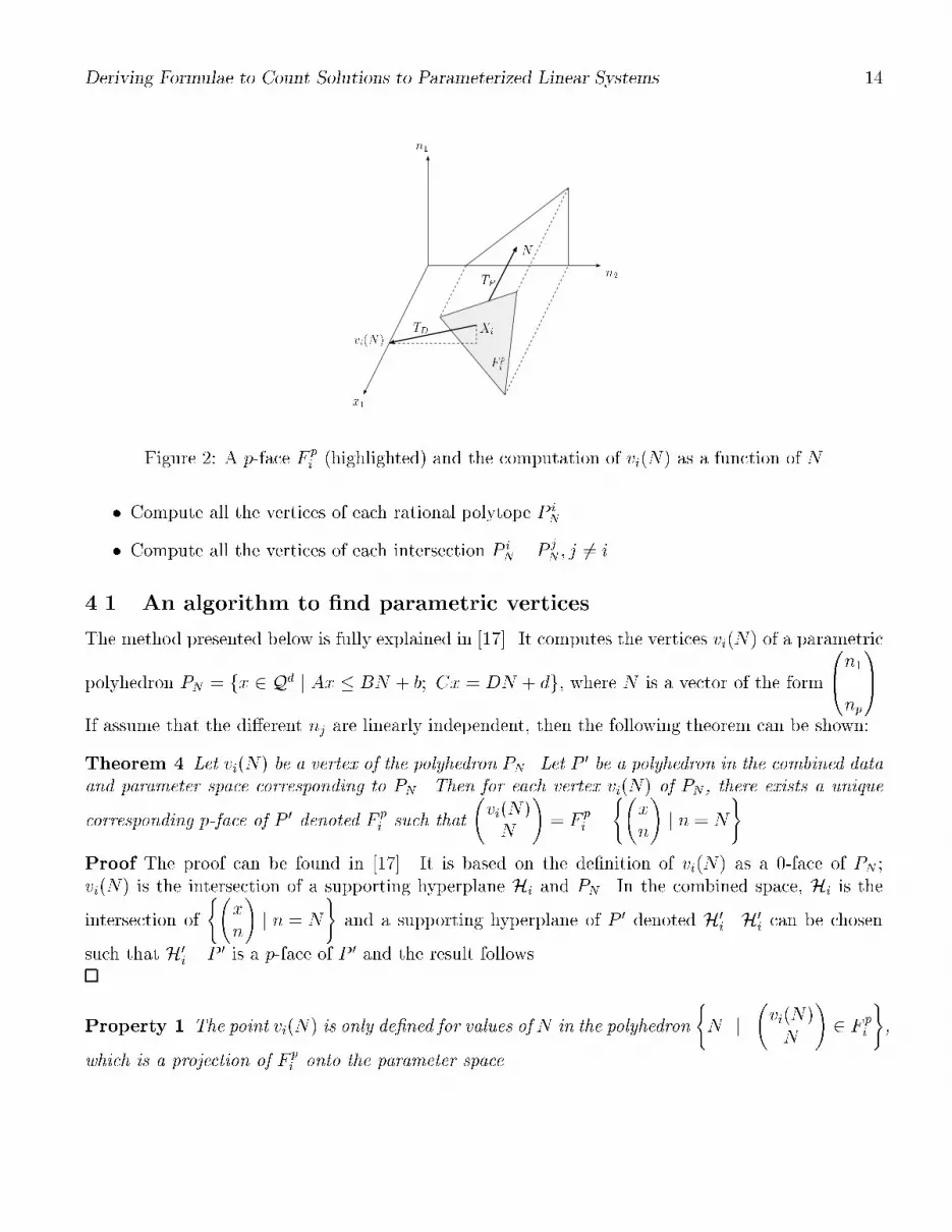
Deriving Formulae to Count Solutions to Parameterized Linear Systems 14n1 n2x1vi(N) NTD TPF piXiFigure 2: A p-face F pi (highlighted) and the computation of vi(N) as a function of N� Compute all the vertices of each rational polytope P iN .� Compute all the vertices of each intersection P iN \ P jN ; j 6= i.4.1 An algorithm to �nd parametric verticesThe method presented below is fully explained in [17]. It computes the vertices vi(N) of a parametricpolyhedron PN = fx 2 Qd j Ax � BN + b; Cx = DN + dg, where N is a vector of the form 0B@n1...np1CA.If assume that the di�erent nj are linearly independent, then the following theorem can be shown:Theorem 4 Let vi(N) be a vertex of the polyhedron PN . Let P 0 be a polyhedron in the combined dataand parameter space corresponding to PN . Then for each vertex vi(N) of PN , there exists a uniquecorresponding p-face of P 0 denoted F pi such that vi(N)N ! = F pi \ ( xn! j n = N).Proof The proof can be found in [17]. It is based on the de�nition of vi(N) as a 0-face of PN ;vi(N) is the intersection of a supporting hyperplane Hi and PN . In the combined space, Hi is theintersection of ( xn! j n = N) and a supporting hyperplane of P 0 denoted H0i. H0i can be chosensuch that H0i \ P 0 is a p-face of P 0 and the result follows.Property 1 The point vi(N) is only de�ned for values of N in the polyhedron (N j vi(N)N ! 2 F pi ),which is a projection of F pi onto the parameter space.

Deriving Formulae to Count Solutions to Parameterized Linear Systems 15Proof Refer to �gure 2. Since vi(N)N ! = F pi \ ( xn! j n = N), the validity domain for vi(N) (therange of N over which vi(N) exists) is (N j vi(N)N ! 2 F pi ). It is a convex polyhedron since it isa projection of F pi and F pi is a convex polyhedron.If F pi is a p-face of P 0 corresponding to a vertex vi(N), then all points vi(N)N ! 2 F pi lie inthe intersection of d = dimension(P 0) � p facets of P 0 and thus must satisfy d linearly independentequations of the form aT vi(N)N ! = c, where a is a constant vector and c is a constant. Using theseequations, we can solve for vi(N) as a vector of linear functions of N .If such a system of equations cannot be solved, then there does not exist one-to-one correspondencebetween points in F pi and values of N . In this case, the p-face F pi not correspond to a vertex of PN ,and that face F pi can be ignored by the algorithm.4.1.1 Partitioning the parameter spaceThe output of the above algorithm is a set of vertices and for each vertex, a set of constraints thatmust be veri�ed by the parameters N for that vertex to be valid.In order to use these results, we need to know the set of distinct parameter subdomains whichpartition complete sets of parameterized vertices, i.e. to transform the collection of (subdomain,vertex) pairs into a collection of (subdomain, set of vertices) pairs, where each subdomain (speci�edby set of conditions on N) is a partition in which a complete set of vertices of PN is stable. Thesepartitions are obtained by intersecting the individual domains of all of the vertices in each set.Ehrhart's theorem (Theorem 1) and our extension to it (Theorem 2) can only be applied tobordered or homothetic polyhedra. These partitions are essential for the application of these theoremsbecause they separate a parameterized polyhedron into a set of bordered and homothetic polyhedra.For each bordered or homothetic polyhedron, a di�erent pseudo-polynomial enumerator is computed.4.2 Computing periodic coe�cientsA pseudo polynomial of degree p� 1 and period q is written:En = [up�1;q�1; � � �up�1;0]n np�1 + [up�2;q�1; � � �up�2;0]n np�2 + � � �+ [u0;q�1; � � �u0;0]n n0The values uj;k ( where 0 � j < p and 0 � k < q) are unknowns. To solve for them, we substitutein di�erent values of n to generate di�erent equations.Normally, a system of pq equations would need to be solved to �nd pq unknown coe�cients takingO(p3n3) time. However, in this case, we can break the problem down and solve p sets of q-equations,which is done in O(pn3) time.Let n = n0 and k = (n0 mod q). Then substituting n for n0 in the pseudo-polynomial, we get:up�1;knp�10 + up�2;knp�20 + � � �+ u0;k = E(n0)If we choose a set of q values for n starting at n0 and then increasing by strides of q, i.e., ni = n0+ iq,0 � i < q, and then substitute those values in the pseudo-polynomial, we arrive at the following

Deriving Formulae to Count Solutions to Parameterized Linear Systems 16system of equations. up�1;knp�10 + up�2;knp�20 + � � �+ u0;k = E(n0)up�1;knp�11 + up�2;knp�21 + � � �+ u0;k = E(n1)...up�1;knp�1q�1 + up�2;knp�2q�1 + � � �+ u0;k = E(nq�1)By striding the value of n by q, the index k = (n mod q) remains constant and the same set of ujkvalues are selected from the periodic coe�cients for each equation. This system of equations can beput into matrix format A~u = ~E as follows:2666664 np�10 np�20 � � � 1np�11 np�21 � � � 1...np�1q�1 np�2q�1 � � � 13777775 266664 up�1;kup�2;k...u0;k 377775 = 266664 E(n0)E(n1)...E(nq�1) 377775Matrix A will always be an integer matrix and the inverse of A will always be a rational matrix. Byinverting matrix A, we can solve for vector ~u, obtaining ~u = A�1 ~E. Two cases arise:1. The E(nj)'s are constant. They are obtained by counting the number of integer points in thepolyhedron P (nj) (nj being a �xed integer). This is done by scanning the polyhedron using thealgorithm described in [16].2. The E(nj)'s are not constant. This happens when the enumerator E is a function of morethan one parameter, E(n;m; � � �). In this case, the enumerator E(nj; m; � � �) is computed bysetting parameter n to nj and recursively calling the procedure to compute the formula forE(m; � � �) = E(n;m; � � �) jn=n0. This recursion will eventually terminate in case 1 when allparameters have been �xed. The recurrent procedure returns a pseudo-polynomial formula andthus the resulting ~E is a vector of pseudo-polynomials. The matrix-vector product A�1 ~E musttherefore be done symbolically and procedures to perform symbolic multiplication and additionof pseudo-polynomials are used to compute uj;k.This entire procedure is then repeated for other sets of values for n, that have di�erent values ofk = (n mod q), until all of the ujk have been solved.4.3 Simplifying pseudo-polynomialsThe pseudo-polynomial returned by the above procedure is not usually in simplest form. A procedurecalled Reduce is called to reduce the pseudo-polynomial E. It is de�ned as follows:Reduce(E)1. If E is not a simple rational number, (it is a polynomial of degree p�1, or a periodicnumber of period p), then for 0 � j < p recursively call Reduce(E:uj).2. If E is a periodic number (E = [up�1; � � � ; u0]), then

Deriving Formulae to Count Solutions to Parameterized Linear Systems 17(a) Try to reduce the period of E.The period of E can be reduced from p to q if9 q : 1 � q < p; pq 2 Z 8 j; c : 0 � j < q; 0 � c < pq (uk = ucq+k)!(b) Try to reduce the strength of E.If the period of E is one (E = [u0]), reduce it from a periodic number to a simple(non-periodic) rational number u0.3. If E is a polynomial (E = up�1xp�1 + up�2xp�2 + � � �+ u0x0), then(a) Try to reduce the degree of E.The degree of E can be reduced from p� 1 to q � 1 if9 q : 1 � q < p (8 j : q � j < p (uj = 0))(b) Try to reduce the strength of E.If the degree of E is zero (E = u0x0), reduce it from a polynomial to a simplerational number u0.Example 7 �34 ; 34 ; 34 ; 34 ; 34 ; 34�n n2 + �12 ; 12 ; 12 ; 12 ; 12 ; 12�n n+ �0;�14 ; 0;�14 ; 0;�14�nis reduced to 34n2 + 12n+ �0;�14�n5 Examples and related workAll the examples considered in this section come from several related works [13, 14, 27, 26, 11, 21]and were also handled by W. Pugh in [21], except example 13 whose aim is to show the generality ofour method.Example 8M. Haghighat and C. Polychronopoulos present a method for volume computation in [13, 14]. Their�rst example is Pni=1Pij=3P5k=j 1. This sum de�nes a set of linear constraints PN = f1 � i � n; 3 �j � i; j � k � 5g. The Loechner/Wilde algorithm computes the following vertices for the polytopePn:� (1) if 3 � n � 5, the vertices are (3; 3; 5), (3; 3; 3), (n; 3; 5), (n; 3; 3), (n; n; 5), (n; n; n).� (2) if n > 5, the vertices are (3; 3; 5), (3; 3; 3), (n; 3; 5), (n; 3; 3), (5; 5; 5), (n; 5; 5).

Deriving Formulae to Count Solutions to Parameterized Linear Systems 18Hence, Pn is an integral 3-polytope and the associated pseudo-polynomial En = c1n3+ c2n2+ c3n+ c4is computed for each of the two domains.Domain 1: From n = 3 to 5 we count En = 3; 8; 14. Since we have only three equations and fourunknowns, we can arbitrarily set c1 to zero, reducing the degree of the polynomial enumerator to 2.The remaining coe�cients are solved for using the following system of equations:(1)8>><>>: c1 = 09c2 + 3c3 + c4 = E3 = 316c2 + 4c3 + c4 = E4 = 825c2 + 5c3 + c4 = E5 = 14The solution of this system results in En = 12n2 + 32n� 6.Our result is di�erent from that computed by Pugh [21], because Pugh only used two points n = 3to 4 where as our algorithm used n = 3 to 5. Both are correct over their respective ranges of n.Domain 2: From n = 5 to 8 we count En = 14; 20; 26; 32.(2)8>><>>: 125c1 + 25c2 + 5c3 + c4 = E5 = 16216c1 + 36c2 + 6c3 + c4 = E6 = 20343c1 + 49c2 + 7c3 + c4 = E7 = 26512c1 + 64c2 + 8c3 + c4 = E8 = 32The solution of this system results in En = 6n� 16.Summary The enumerator is thusEn = ( 12n2 + 32n� 6 if 3 � n � 56n� 16 if 5 � nThis is equivalent to the result derived by W. Pugh. On the other hand, M. Haghighat and C.Polychronopoulos derived the enumerator:�(min(n� 2; 3))(�(min(n; 5))3 + 15(min(n; 5))2 � 38min(n; 5) + 24)=6 + 6max(n� 5; 0)where �(x) is de�ned to be 1 if x is positive and 0 otherwise. The enumerator evaluates to the samevalues as ours, but the form is quite di�erent, and more complicated, because of the �(x), min andmax functions they employ. Our method never generates �(x), min or max functions.Example 9The second example in [13, 14] is 2nXi=1 min(i;2n�i)Xj=1 1This sum de�nes a set of linear constraints Pn = f1 � i � 2n; 1 � j � i; i + j � 2ng. TheLoechner/Wilde algorithm computes the following vertices for the polytope Pn:� if n � 1, the vertices are (n; n); (2n� 1; 1); (1; 1).Hence, Pn is an integral 2-polytope and the associated pseudo-polynomial enumerator En =c1n2 + c2n + c3 is formulated.

Deriving Formulae to Count Solutions to Parameterized Linear Systems 19From n = 1 to 3 we count En = 1; 4; 9. We solve for the unknown coe�cients using the followingsystem of equations: 8<: c1 + c2 + c3 = E1 = 14c1 + 2c2 + c3 = E2 = 49c1 + 3c2 + c3 = E3 = 9The solution of this system results in En = n2, which is the same result as W. Pugh. In [13, 14],Haghighat and Polychronopoulos do not describe their technique in detail. They de�ne a number ofrules in order to transform expressions, but nothing is said on how to decide which rule to apply andwhen. As in [27], they assume the summation must be performed in a predetermined order.Example 10We now handle Pugh's "more elaborate" example of [21], and show that our method does not en-counter any di�culty whatsoever, while Pugh had to introduce additional techniques which were notelaborated in his paper. This example is the set of linear constraints Pn = f1 � i; j � n; 2i � 3jg.The Loechner/Wilde algorithm computes the following vertices for the so-de�ned polytope Pn:� if n � 23 , the vertices are (3n2 ; n); (1; 23); (1; n)Hence, Pn is a rational 2-polytope with a denominator of 6. The associated enumerator is a pseudo-polynomial of degree 2 and period 6:En = [c1; c2; c3; c4; c5; c6]n2 + [c7; c8; c9; c10; c11; c12]n + [c13; c14; c15; c16; c17; c18]From n = 1 to 18 we count En = 1, 4, 8, 14, 21, 30, 40, 52, 65, 80, 96, 114, 133, 154, 176, 200, 225,252. The 18 equations are solved as 6 systems of 3 equations a piece:8<: c2 + c8 + c14 = E1 = 149c2 + 7c8 + c14 = E7 = 40169c2 + 13c8 + c14 = E13 = 133 8<: 4c3 + 2c9 + c15 = E2 = 464c3 + 8c9 + c15 = E8 = 52196c3 + 14c9 + c15 = E14 = 1548<: 9c4 + 3c10 + c16 = E3 = 881c4 + 9c10 + c16 = E9 = 65225c4 + 15c10 + c16 = E15 = 176 8<: 16c5 + 4c11 + c17 = E4 = 14100c5 + 10c11 + c17 = E10 = 80256c5 + 16c11 + c17 = E16 = 2008<: 25c6 + 5c12 + c18 = E5 = 21121c6 + 11c12 + c18 = E11 = 96289c6 + 17c12 + c18 = E17 = 225 8<: 36c1 + 6c7 + c13 = E6 = 30144c1 + 12c7 + c13 = E12 = 114324c1 + 18c7 + c13 = E18 = 252The solution of these systems results inEn = �34 ; 34 ; 34 ; 34 ; 34 ; 34�n n2 + �12 ; 12 ; 12 ; 12 ; 12 ; 12�n n+ ��14 ; 0;�14 ; 0;�14 ; 0�nwhich can be directly simpli�ed to En = 34n2 + 12n+ ��14 ; 0�nPugh [21] uses a di�erent technique to derive an enumerator of( (n+n mod 2)(3n+3(n mod 2)�2)8 if 1 � n3(n�n mod 2)(n�n mod 2+2)8 if 2 � n

Deriving Formulae to Count Solutions to Parameterized Linear Systems 20This expression is then intuitively simpli�ed to 3n2+2n�n mod 24 which evaluates to the same values asour pseudo-polynomial enumerator. This example shows that Pugh's technique tended to complicateanswers when considering rational polytopes, and hence, does not allow to consider systematicallyany set of rational linear constraints. Our method has no di�culty handling any set of rational linearconstraints without any restriction.The method described by Pugh in [21] consists of a set of tools and techniques dedicated tosimplifying the initial set of constraints. Applying all of these tools could be expensive for large setsof constraints with rational coe�cients. Moreover, their application is often rule driven, in some casesinvolving the addition of auxiliary variables and the use of standard formulas for sums of powers.(Pugh expects it will be su�cient to hard code the formulas for powers up to 10.) And �nally, theresulting formula involves the use of modulo functions. This shows some of the limitations in thegeneral use of Pugh's method.6 Application to the analysis of nested-loop programsIn this section, we give several examples of how the method is applied to applications which need toanalyze nested-loops.Example 11An example in [11] asks to calculate the number of memory locations touched in a Successive Over-Relaxation (SOR) code:for i := 2 to n-1 dofor j := 2 to n-1 doa(i,j) = (2*a(i,j) + a(i-1,j) + a(i+1,j)+ a(i,j-1) + a(i,j+1)) / 6The elements of a touched by this loop aref(i; j)j2 � i; j � n� 1g[ f(i� 1; j)j2 � i; j � n� 1g[ f(i+ 1; j)j2 � i; j � n� 1g[ f(i; j � 1)j2 � i; j � n� 1g[ f(i; j + 1)j2 � i; j � n� 1g = f(i; j)j2 � i; j � n� 1g[ f(i; j)j1 � i � n� 2; 2 � j � n� 1g[ f(i; j)j3 � i � n; 2 � j � n� 1g[ f(i; j)j2 � i � n� 1; 1 � j � n� 2g[ f(i; j)j2 � i � n� 1; 3 � j � ngThe parametric vertices of this union of polytopes Pn are computed by using the heuristic proceduredescribed in subsection 4.1. It gives the following results: (1; 2), (2; 1), (1; n � 1), (2; n), (n � 1; n),(n; n � 1), (n � 1; 1) and (n; 2). Hence, it is an integral 2-polytope and the associated Ehrhartpolynomial is En = c1n2 + c2n+ c3.From n = 4 to 6 we count En = 12; 21; 32.8<: 16c1 + 4c2 + c3 = E4 = 1225c1 + 5c2 + c3 = E5 = 2136c1 + 6c2 + c3 = E6 = 32The solution of this system gives the result En = n2 � 4 which is the same answer that Pugh gave.

Deriving Formulae to Count Solutions to Parameterized Linear Systems 21Example 12An extension of our method to several size parameters has been implemented. It is applied toan example handled by Tawbi in [26] which is Pni=1Pij=1Pmk=j 1. This sum de�nes a set of linearconstraints f1 � i � n; 1 � j � i; j � k � mg. The Loechner/Wilde algorithm computes thefollowing vertices for the so-de�ned polytope Pn;m:� (1) if 1 � n � m, the vertices are (1; 1; m), (1; 1; 1), (n; 1; m), (n; 1; 1), (n; n;m), (n; n; n).� (2) if 1 � m � n, the vertices are (1; 1; m), (1; 1; 1), (n; 1; m), (n; 1; 1), (m;m;m), (n;m;m).Hence, Pn;m is an integral 3-polytope and the associated pseudo-polynomial is of the form En;m =P3i=0P3�ij=0 cijnimj and has to be computed for each of the two domains, (1) and (2).Domain 1: Our method, applied to several size parameters, uses a symbolic resolution by �rstconsidering the polynomial En;m = d3(m)n3 + d2(m)n2 + d1(m)n + d0(m) where:d3(m) = c33m3 + c32m2 + c31m+ c30d2(m) = c23m3 + c22m2 + c21m+ c20d1(m) = c13m3 + c12m2 + c11m+ c10d0(m) = c03m3 + c02m2 + c01m+ c00Symbolically evaluating En;m at n = 1; 2; 3; 4, yields the following symbolic system of equations.8>>><>>>: d3(m) + d2(m) + d1(m) + d0(m) = E1;m8d3(m) + 4d2(m) + 2d1(m) + d0(m) = E2;m27d3(m) + 9d2(m) + 3d1(m) + d0(m) = E2;m64d3(m) + 16d2(m) + 4d1(m) + d0(m) = E4;mIn order to solve for the symbolic coe�cients d3(m), d2(m), d1(m), and d0(m), the enumeratorsE1;m, E2;m, E3;m and E4;m have to be computed.For n = 1 and from m = 1 to 4, we count En;m = 1; 2; 3; 4.8>>><>>>: c1 + c2 + c3 + c4 = E1;1 = 18c1 + 4c2 + 2c3 + c4 = E1;2 = 227c1 + 9c2 + 3c3 + c4 = E1;3 = 364c1 + 16c2 + 4c3 + c4 = E1;4 = 4This system results in E1;m = m. In the same way, we compute E2;m = 3m� 1, E3;m = 6m� 4 andE4;m = 10m� 10, giving the equations8>>><>>>: d3(m) + d2(m) + d1(m) + d0(m) = m8d3(m) + 4d2(m) + 2d1(m) + d0(m) = 3m� 127d3(m) + 9d2(m) + 3d1(m) + d0(m) = 6m� 464d3(m) + 16d2(m) + 4d1(m) + d0(m) = 10m� 10The expressions for d1(m); d2(m); d3(m) and d4(m) can be symbolically computed as: d1 = �16 ,d2 = m2 , d3 = m2 + 16 and d4 = 0. Thus, for domain 1 � n � m, the enumerator En;m is derived as:En;m = �16n3 + m2 n2 + (12m+ 16)n + 0= �n36 + n2m2 + nm2 + n6

Deriving Formulae to Count Solutions to Parameterized Linear Systems 22Domain 2: The same work is done for domain (2), i.e. 1 � m � n, resulting in En;m = �m36 +m2n2 +mn2 +m6 , which matches the result of Pugh. Our method can be applied the same way when consideringseveral size parameters in the case of rational polytopes, case which is not systematically handledby Pugh's techniques. Tawbi in [27, 26] �rst used a polyhedral splitting technique to characterizethe de�nition domains, and an elimination of the variables in a predetermined order. However, hermethod does not allow systematically computing exact formulae like our method.Example 13We propose a more complex example than any previously published, requiring the use of the entiremethod we have described. This example involves rational parameterized polytopes depending onthree size parameters. Let us consider the following loop nest:for i := 0 to n dofor j := 0 to i + m/2 dofor k := 0 to i - n + p doa(i,j,k) = a(i,j,k-1) + a(k,j,k)*a(i,k,k)We want to compute the number of ops in order to evaluate the execution time of this code segment.This loop nest is modeled by the convex polytope PN = fz 2 Z3 j Az � BN + Cg whereA=0BBBBBBBB@ �1 0 01 0 00 �1 0�2 2 00 0 �1�1 0 1

1CCCCCCCCA B =0BBBBBBBB@ 0 0 01 0 00 0 00 1 00 0 0�1 0 11CCCCCCCCA N =0B@ nmp 1CA C = 0BBBBBBBB@ 000000

1CCCCCCCCAThe Loechner/Wilde algorithm computes the following vertices for the so-de�ned polytope PN :� (1) if n � p: (n� p; 2n+m�2p2 ; 0), (n� p; 0; 0), (n; 2n+m2 ; p), (n; 2n+m2 ; 0), (n; 0; p), (n; 0; 0).� (2) if n � p: (0; m2 ;�n+ p), (0; m2 ; 0), (0; 0;�n+ p), (0; 0; 0), (n; 2n+m2 ; p), (n; 2n+m2 ; 0), (n; 0; p), (n; 0; 0).As an example, we now compute the pseudo-polynomial enumerator on the �rst de�nition domain.The denominator of PN is 2. We count ((k + 1)d)q = 512 initial values of E(n;m; p). The lowestinitial value of n is 9 since we consider the �rst de�nition domain (n � p) and since for any initialvalue of n, 8 initial values of p have to be considered. For example, with n = 9 we get the followinginitial counts: n=9 p 1 2 3 4 5 6 7 8m1 29 56 90 130 175 224 276 3302 32 62 100 145 196 252 312 3753 32 62 100 145 196 252 312 3754 35 68 110 160 217 280 348 4205 35 68 110 160 217 280 348 4206 38 74 120 175 238 308 384 4657 38 74 120 175 238 308 384 4658 41 80 130 190 259 336 420 510

Deriving Formulae to Count Solutions to Parameterized Linear Systems 23Each line of this array allows resolving a system of equations to determine E(x; y; p), for all x 2[9::16] and y 2 [1::8]. For example, the �rst system dedicated to the determination of E(9; 1; p) =[c2; c1]p n33 + [c4; c3]p n23 + [c6; c5]p n3 + [c8; c7]p isn = 9; m = 1 : 8>>>>>>>>>><>>>>>>>>>>:p = 1 : c1 + c3 + c5 + c7 = 29p = 2 : 8c2 + 4c4 + 2c6 + c8 = 56p = 3 : 27c1 + 9c3 + 3c5 + c7 = 90p = 4 : 64c2 + 16c4 + 4c6 + c8 = 130p = 5 : 125c1 + 25c3 + 5c5 + c7 = 175p = 6 : 216c2 + 36c4 + 6c6 + c8 = 224p = 7 : 343c1 + 49c3 + 7c5 + c7 = 276p = 8 : 512c2 + 64c4 + 8c6 + c8 = 330resulting in E(9; 1; p) = �16p3 + 92p2 + 443 p+ 10.Solving for the other polynomials, E(9; 2; p) : : : E(9; 8; p), allows resolving systems to determineE(9; m; p) = [c2; c1]mm3 + [c4; c3]mm2 + [c6; c5]mm+ [c8; c7]m with this system of equations:

n = 9 : 8>>>>>>>>>><>>>>>>>>>>:m = 1 : c1 + c3 + c5 + c7 = � 16p3 + 92p2 + 443 n3 + 10m = 2 : 8c2 + 4c4 + 2c6 + c8 = � 16p3 + 5p2 + 976 p+ 11m = 3 : 27c1 + 9c3 + 3c5 + c7 = � 16p3 + 5p2 + 976 p+ 11m = 4 : 64c2 + 16c4 + 4c6 + c8 = � 16p3 + 112 p2 + 533 p+ 12m = 5 : 125c1 + 25c3 + 5c5 + c7 = � 16p3 + 112 p2 + 533 p+ 12m = 6 : 216c2 + 36c4 + 6c6 + c8 = � 16p3 + 6p2 + 1156 p+ 13m = 7 : 343c1 + 49c3 + 7c5 + c7 = � 16p3 + 6p2 + 1156 p+ 13m = 8 : 512c2 + 64c4 + 8c6 + c8 = � 16p3 + 132 p2 + 623 p+ 14In this case, the following result is obtained:E(9; m; p) = 14mp2 + 34mp + 12m� 16p3 + h92 ; 174 im p2 + h443 ; 16712 im p+ h10; 192 imIn a similar way, E(10; m; p), E(11; m; p), . . . , E(16; m; p) are computed. Finally, E(n;m; p) isdetermined by resolving the system shown below:8>>>>><>>>>>: n = 9 : 729c1 + 81c3 + 9c5 + c7 = 14mp2 + 34mp + 12m � 16 p3 + [ 92 ; 174 ]mp2 + [ 443 ; 16712 ]mp+ [10; 192 ]mn = 10 : 1000c2 + 100c4 + 10c6 + c8 = 14mp2 + 34mp + 12m � 16 p3 + [5; 194 ]mp2 + [ 976 ; 18512 ]mp+ [11; 212 ]mn = 11 : 1331c1 + 121c3 + 11c5 + c7 = 14mp2 + 34mp + 12m � 16 p3 + [ 112 ; 214 ]mp2 + [ 533 ; 20312 ]mp+ [12; 232 ]mn = 12 : 1728c2 + 144c4 + 12c6 + c8 = 14mp2 + 34mp + 12m � 16 p3 + [6; 234 ]mp2 + [ 1156 ; 22112 ]mp+ [13; 252 ]mn = 13 : 2197c1 + 169c3 + 13c5 + c7 = 14mp2 + 34mp + 12m � 16 p3 + [ 132 ; 254 ]mp2 + [ 623 ; 23912 ]mp+ [14; 272 ]mn = 14 : 2744c2 + 196c4 + 14c6 + c8 = 14mp2 + 34mp + 12m � 16 p3 + [7; 274 ]mp2 + [ 1336 ; 25712 ]mp+ [15; 292 ]mn = 15 : 3375c1 + 225c3 + 15c5 + c7 = 14mp2 + 34mp + 12m � 16 p3 + [ 152 ; 294 ; ]mp2 + [ 713 ; 27512 ]mp+ [16; 312 ]mn = 16 : 4096c2 + 256c4 + 16c6 + c8 = 14mp2 + 34mp + 12m � 16 p3 + [8; 314 ]mp2 + [ 1516 ; 29312 ]mp+ [17; 332 ]mThe following result is obtained, giving the number of ops executed by the loop nest when n � p:E(n;m; p) = 12np2 + 32np+ n+ 14mp2 + 34mp+ 12m� 16p3 + �0;�14�m p2 + �76 ; 512�m p+ �1; 12�mLikewise, when n � p:E(n;m; p) = � 16n3 � 14n2m+ n2 � 12p; 12p� 14�m + 12nmp+ 14nm+ n �32p+ 76 ; p+ 1112�m + 12mp+ 12m+ �p+ 1; 12p+ 12�mExample 14For our last example, we show an application of parametric analysis. We derive the maximum amountof parallelism found in a small nested-loop program.Consider the following loop nest:

Deriving Formulae to Count Solutions to Parameterized Linear Systems 24jik

v2v3 v1Figure 3: Tn;t0 in the �rst validity domain

jik

v2v3 v5 v4

Figure 4: Tn;t0 in the second validity domainfor i:= 0 to n dofor j:= 0 to i dofor k:= 0 to i-j doStatement(s)This loop nest is modeled by the one-parameter polyhedral iteration space de�ned by:Pn = f� ijk� 2 Z3j0B@ �1 0 01 0 00 �1 0�1 1 00 0 �1�1 1 1 1CA� ijk� � 0B@ 010000 1CAngAssume that the dependence analysis of this loop nest yields an optimal linear schedule de�ned byt(i; j; k) = i + j + k: any iteration (i; j; k) is computed at instant i + j + k. We use our methodto determine the parametric number of simultaneous calculations par(n; t0) occuring at any instantt0, in order to determine the parametric maximum parallelism maxpar(n) =MAXt0fpar(n; t0)g, i.e.the maximum number of simultaneous calculations.From a geometrical point of view, all the points (i; j; k) of Pn resulting in the same value oft0 = t(i; j; k), belong to the two-parameters rational 2-polytope Tn;t0 de�ned by Tn;t0 = Pn\f(i; j; k) 2Z3ji+ j + k = t0g. The number of points in Tn;t0 is par(n; t0).Giving this last parametric de�nition of Tn;t0 as an input to the parametric vertices �nding algo-rithm, it outputs the following results as shown on �gures 3 and 4:� if 0 � t0 � n, the parametric vertices are v1 = (t0; 0; 0), v2 = � t02 ; t02 ; 0� and v3 = � t02 ; 0; t02 �.� if n � t0 � 2n, the parametric vertices are v2 = � t02 ; t02 ; 0�, v3 = � t02 ; 0; t02 �, v4 = (n; t0 � n; 0)and v5 = (n; 0; t� n).� otherwise, Tn;t0 does not exist and par(n; t0) = 0.Hence, par(n; t0) is de�ned on two validity domains as pseudo-polynomials in n and t0, of degree2, and of pseudo-period 2. According to theorem 3 and by looking at T1;0, it is deduced that all thecoe�cients of nq, q � 2, are constant: par(n; t0) = c1n2 + c2n + c3.

Deriving Formulae to Count Solutions to Parameterized Linear Systems 25(i) We determine c1; c2; c3 by solving the following system of equations on the �rst validity domain:8><>: 36c1 + 6c2 + c3 = par(6; t0)49c1 + 7c2 + c3 = par(7; t0)64c1 + 8c2 + c3 = par(8; t0)Solving this system yields the equations for par(6; t0), par(7; t0) and par(8; t0). According to theorem3 and by looking at T1;1, it is deduced that only the coe�cient of t20 is constant. For example,par(6; t0) = c1t20 + [c3; c2]t0 + [c5; c4], such that:8>>>>>><>>>>>>: c5 = par(6; 0) = 1c1 + c2 + c4 = par(6; 1) = 14c1 + 2c3 + c5 = par(6; 2) = 39c1 + 3c2 + c4 = par(6; 3) = 316c1 + 4c3 + c5 = par(6; 4) = 6where the values of par(6; 0); : : : ; par(6; 4) are given by some initial counts.) par(6; t0) = 18t20+[34 ; 12 ]t0+[1; 38 ]. In the same way, we determine that the other pseudo-polynomialsare the same, i.e 8 n 2 [6::8]; par(n; t0) = 18t20 + [34 ; 12 ]t0 + [1; 38 ]. Solving the �rst system gives theparallelism rate of any instant t0 on the �rst validity domain:8 0 � t0 � n; par(n; t0) = 18t20 + h34 ; 12i t0 + h1; 38iObserve that the parallelism rate does not depend on n in this validity domain.(ii) We now consider the second validity domain.8><>: 36c1 + 6c2 + c3 = par(6; t0)49c1 + 7c2 + c3 = par(7; t0)64c1 + 8c2 + c3 = par(8; t0)Solving this system yields the equations for par(6; t0), par(7; t0) and par(8; t0). For example,par(6; t0) = c1t20 + [c3; c2]t0 + [c5; c4], such that:8>>>>>><>>>>>>: 36c1 + 6c3 + c5 = par(6; 6) = 1049c1 + 7c2 + c4 = par(6; 7) = 964c1 + 8c3 + c5 = par(6; 8) = 1281c1 + 9c2 + c4 = par(6; 9) = 9100c1 + 10c3 + c5 = par(6; 10) = 11) par(6; t0) = �38 t20 + [254 ; 6]t0 + [�14;�1178 ]. In the same way, we determine the other pseudo-polynomials: par(7; t0) = �38 t20 + [294 ; 7]t0 + [�20;�1658 ]par(8; t0) = �38 t20 + [334 ; 8]t0 + [�27;�2218 ]Solving the �rst system gives the parallelism rate of any instant t0 on the second validity domain:8 n � t0 � 2n; par(n; t0) = nt0 � 12n2 + 12n� 38 t20 + h 14 ; 0it0 t0 � h1; 38it0(iii) From these results, the maximum parallelism is deduced:

Deriving Formulae to Count Solutions to Parameterized Linear Systems 26� On the �rst validity domain (0 � t0 � n), par(n; t0) is maximum when t0 is maximum, i.e.when t0 = n. Hence, maxpar(n) = 18n2 + h34 ; 12in+ h1; 38i.� On the second validity domain (n � t0 � 2n), we take the derivative of par(n; t0) with respectto t0: par0(n; t0) = n� 34 t0 + h14 ; 0it0 . par0(n; t0) � 0, n� 34t0 + h0; 14it0 � 0, t0 � 4n�[1;0]3Hence, par(n; t0) increases from t0 = n to t0 = 4n�[1;0]3 , and then decreases until t0 = 2n: it ismaximum for t0 = tmax = 4n�[1;0]3 . Since tmax is not always integral, a case study is necessaryto get the exact value of maxpar(n) = par(n; tmax), checking the possible values of btmaxc anddtmaxe. It yields the following answer: maxpar(n) = 16n2 + 56n� h1; 1; 2324i.� In conclusion, the maximum parallelism of the loop nest is:8 n � 0; maxpar(n) = 16n2 + 56n� h1; 1; 2324i7 Non-linear extensionsAll these results concern normal polyhedra de�ned by a combination of linear constraints. Whenconsidering some nonlinear ones, the transformation rules given in this section have to be applied�rst.This set of constraints depends on some positive integral size parameters. Any constraint Ck is ofthe form Ck :Xi ai�i �Xj bjnj + cwhere the ai's, bi's and c are rational constants, the nj's are the size parameters and the �i's can beof the form xi (xi mod di) bxidi c dxidi e (dijxi)where di is an integral constant, (dijxi) means that di evenly divides xi and xi is any rational linearcombination of the free variables. When the form of any �i yields a nonlinear constraint, this caneasily be transformed into a linear one through some elementary transformations, as those presentedby W. Pugh in [21]:� If a term bxidi c appears in Ck, a free variable z is added to the set of free variables, and constraintCk is replaced with fdiz � xi < di(z + 1); C 0kg where C 0k is Ck with bxidi c replaced with z.� If a term dxidi e appears in Ck, a free variable z is added to the set of free variables, and constraintCk is replaced with fdi(z � 1) < xi � diz; C 0kg where C 0k is Ck with dxidi e replaced with z.� If a term (xi mod di) appears in Ck, a free variable z is added to the set of free variables, andconstraint Ck is replaced with fdiz � xi < di(z + 1); C 0kg where C 0k is Ck with (xi mod di) replacedwith xi � z.

Deriving Formulae to Count Solutions to Parameterized Linear Systems 27� A constraint (dijxi) is equivalent to (xi mod di = 0) and the precedent rule can be applied.� If a term of the form bUu c appears in the right side of the constraint Ck, since rational constraintsare considered by our method, the oor can be avoided and the whole constraint is multiplied by u.8 ConclusionWe have presented a general method, based on the vertices of parameterized polytopes and Ehrhartpolynomials, for deriving a symbolic formula for the number of integer solutions to a set of parameter-ized linear constraints. The enumerator is formulated symbolically as a pseudo-polynomial in termsof parameters, The method we have presented is robust and handles any set of rational parameterizedlinear constraints without any restriction. Moreover, the method gives a closed form formula whicheasily evaluates to exact counts. The procedure is entirely computable and has been implementedalong with the parametric vertices �nding algorithm of Loechner and Wilde [17] and operates inassociation with the polyhedral library [28].Being able to �nd symbolic enumerators has many applications in the analysis and transformationof scienti�c programs. We have given several examples in this paper. There are many other appli-cations in the analysis and transformation of loop nests, some of which can be found in works citedhere above or in [4, 5]. Other applications may also be found in other �elds as sequential programanalysis, combinatorics and optimization.We have compared our method with other similar methods. M. Haghighat and C. Polychronopou-los present in [13, 14] a method for volume computation. The form of their answers is di�erent becauseof the min and max expressions they introduce. Their results tend to be more complicated.Ferrante, Sarkar and Thrash in [11] present methods for computing the number of distinct memorylocations and cache lines accessed by a loop nest. These methods cannot handle unions of polytopes,do not compute symbolic answers, often compute only an approximation, and use expensive methodsto handle the cache lines touched by a set of references.The method described by Pugh in [21] consists of a set of tools and techniques dedicated tosimplifying the initial set of constraints. Applying all of these tools could be expensive for large setsof constraints with rational coe�cients. Moreover, their application is often rule driven, in some casesinvolving the addition of auxiliary variables and the use of standard formulas for sums of powers.(Pugh expects it will be su�cient to hard code the formulas for powers up to 10.) And �nally, theresulting formula involves the use of modulo functions.Tawbi in [27, 26] �rst uses a polyhedral splitting technique to characterize the validity domains,and an elimination of the variables in a predetermined order. However, her method does not system-atically compute exact answers.After doing these comparisons, we make these observations:� summations over several variables should not presume an order in which to perform the sum-mation (as pointed out by Pugh in [21]),� a general technique must also consider rational polytopes, since nested loops models often yieldrational a�ne loop bounds, and since it is useful to systematically handle a wide variety ofapplications in the parallelization of scienti�c programs.

Deriving Formulae to Count Solutions to Parameterized Linear Systems 28� in order to be simple, the result should be expressed without any complex function as min's,max's, mod's, oors or ceilings. In this respect, periodic numbers, introduced by Ehrhart [10],are a good alternative and can undoubtedly be used in other situations.� exact formulations can be found.This is the �rst method to be proposed that enumerates both integer and rational polytopes usinga single comprehensive algorithm. Moreover, the formulation, using Ehrhart pseudo-polynomials, issimple and gives exact parametric expressions for the number of integer points.References[1] A. I. Barvinok. A polynomial-time algorithm for counting integral points in polyhedra whenthe dimension is �xed. In Proc. of the 34th Symp. on the Foundations of Computer Science(FOCS'93), pages 566-572. IEEE Computer Society Press, New York, 1993.[2] A. I. Barvinok. Computing the Ehrhart Polynomial of a Convex Lattice Polytope. DiscreteComput. Geom., 12:35-48,1994.[3] M.S. Bazaraa, H.D. Sherali and C.M. Shetty. Nonlinear Programming, Theory and Algorithms,second edition. Wiley, New York, 1993.[4] Ph. Clauss. The volume of a lattice polyhedron to enumerate processors and parallelism. ResearchReport ICPS 95-11, 1995. http://icps.u-strasbg.fr/pub-95/pub-95-11.ps.gz[5] Ph. Clauss. Counting Solutions to Linear and Nonlinear Constraints through Ehrhart poly-nomials: Applications to Analyze and Transform Scienti�c Programs. 10th ACM Int. Conf.on Supercomputing, Philadelphia, May 1996. Also available as Research Report ICPS 95-20.http://icps.u-strasbg.fr/pub-96/pub-95-20.ps.gz[6] M. Dyer and A. M. Frieze. On the complexity of computing the volume of a polyhedron. SIAMJ. Comput., 17(5):967-974, 1988.[7] E. Ehrhart. Sur les poly�edres rationnels homoth�etiques �a n dimensions. C.R. Acad. Sci. Paris,254:616-618, 1962.[8] E. Ehrhart. Sur un probl�eme de g�eom�etrie diophantienne lin�eaire I. J. Reine Angew. Math.,226:1-29, 1967.[9] E. Ehrhart. Sur un probl�eme de g�eom�etrie diophantienne lin�eaire II. J. Reine Angew. Math.,227:25-49, 1967.[10] E. Ehrhart. Polynomes arithm�etiques et M�ethode des Poly�edres en Combinatoire. InternationalSeries of Numerical Mathematics, vol.35, Birkh�auser Verlag, Basel/Stuttgart, 1977.[11] J. Ferrante, V. Sarkar and W. Thrash. On estimating and enhancing cache e�ectiveness. Advancesin Languages and Compilers for Parallel Processing, pages 328-343. The MIT Press, 1991.[12] P.M. Gruber and C.G. Lekkerkerker. Geometry of Numbers. North-Holland, Amsterdam, 1987.

Deriving Formulae to Count Solutions to Parameterized Linear Systems 29[13] M. Haghighat and C. Polychronopoulos. Symbolic analysis: A basis for parallelization, opti-mization and scheduling of programs. U. Banerjee et al., editor, Languages and Compilers forParallel Computing. Springer-Verlag, August 1993. LNCS 768, Proc. of the 6th annual workshopon Programming Languages and Compilers for Parallel Computing.[14] M. Haghighat and C. Polychronopoulos. Symbolic analysis: A basis for parallelization, opti-mization and scheduling of programs. Technical Report 1317, CSRD, Univ. of Illinois, August1993.[15] D. J. Kuck. The Structure of Computers and Computations, J. Wiley and Sons, N.Y., 1978.[16] H. Le Verge, V. Van Dongen, and D. Wilde. La synth�ese de nids de boucles avec la biblioth�equepoly�edrique. RenPar`6, Jun 1994. English version \Loop Nest Synthesis Using the PolyhedralLibrary" in IRISA technical report 830, May 1994.[17] V. Loechner and D. K. Wilde. Parameterized polyhedra and their vertices. Research Report ICPS96-09, Submitted for publication, 1996. http://icps.u-strasbg.fr/pub-96/pub-96-09.ps.gz[18] I. G. Macdonald. The volume of a lattice polyhedron. Proc. Camb. Phil. Soc., 59:719-726, 1963.[19] I. G. Macdonald. Polynomials associated with �nite cell-complexes. J. London Math. Soc.,4(2):181-192, 1971.[20] T. H. Mattheiss and D. Rubin. A survey and comparison of methods for �nding all vertices ofconvex polyhedral sets. Mathematics of Operations Research, 5(2):167-185, 1980.[21] W. Pugh. Counting Solutions to Presburger Formulas: How and Why. Proc. of the 1994 ACMSIGPLAN Conference on Programming Language Design and Implementation, 1994.[22] A. Schrijver. Theory of Linear and Integer Programming. Wiley, New York, 1986.[23] H. S. Stone and D. Thiebaut. Footprints in the cache. Proc. ACM SIGMETRICS 1986, pp. 4-8,May 1986.[24] R. P. Stanley. Combinatorics and Commutative Algebra. Birkh�auser, Boston, 1983.[25] R. P. Stanley. Enumerative Combinatorics Volume I. Wadsworth & Brooks/Cole, Monterey,California, 1986.[26] N. Tawbi. Estimation of nested loop execution time by integer arithmetics in convex polyhedra.Proc. of the 1994 International Parallel Processing Symposium, April 1994.[27] N. Tawbi and P. Feautrier. Processor allocation and loop scheduling on multiprocessor computers.Proc. of the 1992 International Conference on Supercomputing, pages 63-71, July 1992.[28] D. K. Wilde. A library for doing polyhedral operations.Master's thesis, Oregon State University,Corvallis, Oregon, Dec 1993. Also published as IRISA technical report PI 785, Rennes, France,Dec 1993.