Inter-American Development Bank Banco Interamericano de Desarrollo (BID)

Research Department Departamento de Investigación

Working Paper #545

Maturity Mismatch and Financial Crises: Evidence from Emerging Market Corporations

by

Hoyt Bleakley* Kevin Cowan**

*University of California at San Diego **Inter-American Development Bank

July 2005

©2005 Inter-American Development Bank 1300 New York Avenue, N.W. Washington, DC 20577 The views and interpretations in this document are those of the authors and should not be attributed to the Inter-American Development Bank, or to any individual acting on its behalf. The Research Department (RES) produces a quarterly newsletter, IDEA (Ideas for Development in the Americas), as well as working papers and books on diverse economic issues. To obtain a complete list of RES publications and read or download them, please visit our web site at: http://www.iadb.org/res

Maturity Mismatch and Financial Crises:

Evidence from Emerging Market Corporations∗

Hoyt Bleakley† Kevin Cowan‡

December 17, 2004

AbstractSubstantial attention has been paid in recent years to the risk of maturity mismatch in

emerging markets. Although this risk is microeconomic in nature, the evidence advanced thus farhas taken the form of macro correlations. We evaluate this mechanism empirically at the microlevel by using a database of over 3000 publicly traded firms from fifteen emerging markets. Wemeasure the risk of short-term exposure by estimating, at the firm level, the effect on investmentof the interaction of short-term exposure and aggregate capital flows. This effect is (statistically)zero, contrary to the prediction of the maturity-mismatch hypothesis. This conclusion is robustto using a variety of different estimators, alternative measures of capital flows, and controls fordevaluation effects and access to international capital. We do find evidence that short-term-exposed firms pay higher financing costs and liquidate assets at “fire sale” prices, but not thatthis reduction in net worth translates into a drop in investment.

Keywords: maturity mismatch, investment, financial crisesJEL Classification: E22, F41, G31, G32

∗The authors thank (without implicating) Camilo Arenas, Peter Garber, Marcio Garcia, Augustin Landier, andOsmel Manzano and seminar participants at the Corporacion Andina de Fomento, the Universidad de los Andes, the2003 LACEA meetings, the 2004 Annual Research Conference at the IMF, and the 2004 meeting of the Latin FinanceNetwork for useful comments; Cesar Serra and Erwin Hansen for excellent research assistance. Bleakley gratefullyacknowledges the Corporacion Andina de Fomento and the Latin American East Asian Business Association forfinancial support. An earlier version of this study was circulated under the title “Maturity Mismatch on the PacificRim: Crises and Corporations in East Asia and Latin America.” All errors and opinions are those of the authors.

†Assistant Professor of Economics, University of California at San Diego, 9500 Gilman Drive #0508, La Jolla,CA, 92093. Telephone: (858) 534-3832. Electronic mail: bleakley[at]ucsd[dot]edu

‡Research Economist, Inter-American Development Bank, 1300 New York Ave NW, Washington, DC, 20577.Telephone: (202) 623-2607. Electronic mail: kevinco[at]iadb[dot]org

1

I Introduction

The risk of “maturity mismatch” for emerging-market firms has received considerable attention in

recent years. Although business assets are (stereotypically) installed for the long term and therefore

illiquid, capital-market frictions and distortions may induce firms to issue debt with relatively short

maturity. Should aggregate credit conditions shift suddenly, these same firms, unable to renew

their debt, might have to curtail investment and perhaps liquidate. On the aggregate level, entire

economies may be at risk of an investment collapse in the event of a capital-account reversal.

Proponents of this view include Radelet and Sachs (1998) and Chang and Velasco (1999), who

argue that excessive reliance on short-term debt leaves emerging-market corporations vulnerable

to “financial panic” as in the stylized model of Diamond and Dybvig (1983).

These discussions were largely inspired by the financial crises that affected East Asia and Latin

America in the 1990s. The idea took on particular poignancy in reference to the emerging markets

of Asia, where the corporate sector was highly leveraged leading up to the crisis, and where much

of this indebtedness was at the short term.

That such a scenario is logically possible is by now beyond doubt. That such a mechanism is

of quantitative importance, however, remains an empirical question. Unfortunately, the “macro”

observation that crises occur with greater frequency in economies that have more short-term in-

debtedness does not constitute sufficient evidence. “Weaker” economies and those exposed to larger

shocks may in equilibrium issue debt at shorter durations. Moreover, in equilibrium, capital flight

will almost mechanically be associated with a decline in investment, but it will not necessarily be

the ultimate or even the proximate cause.

Instead, we examine this mechanism at the micro level by examining the behavior of corporate

investment. This analysis involves comparing firms that face the same shift in aggregate credit

conditions, but differ in their potential exposure. According to the maturity-mismatch hypothesis,

firms with excessive short-term debt should suffer most from the aggregate capital outflow.

We assemble a database with accounting information (including the maturity composition of

liabilities) for approximately 3000 publicly traded non-financial firms in emerging markets. The

countries represented in this sample consist of five East Asian countries (Indonesia, Malaysia,

Philippines, South Korea, and Thailand), seven Latin American countries (Argentina, Brazil, Chile,

Colombia, Mexico, Peru and Venezuela) and three additional emerging markets (Israel, South

Africa, and Turkey). These data cover some of the largest emerging markets for 1990’s, a period

2

of substantial capital-account volatility for most of these countries. In addition, there are firms in

our sample that hold substantial amounts of short-term debt. These elements constitute the two

ingredients necessary for examining the proposed mechanism. The choice of publicly listed firms

is determined exclusively by the availability of accounting data. Moreover, we concentrate on the

non-financial sector of the economy, as it is here that investment decisions are ultimately carried

out.

The specific empirical strategy is to assess whether firms with more short-term exposure invest

less in the aftermath of capital flight. We do so by estimating reduced-form equations for investment.

The proposed mechanism centers on the interaction of short-term indebtedness with capital flows,

and so the key variable in the analysis is

( Short-Term Exposure )i,t−1 × ( Capital Flows )t

for firm i at time t. This analysis allows us to better understand whether the marginal unit of

debt is allocated across firms in such a way as to generate the large risk suggested by the maturity-

mismatch hypothesis. The hypothesis is that we should estimate a strong and positive effect of this

interaction.

The main empirical result is that the investment response of relatively short-term-exposed firms

to aggregate capital flows is statistically indistinguishable from that of firms that hold predomi-

nantly long-term debt. This finding is robust to the inclusion of controls for preexisting firm

differences as well as to the interaction of these controls with aggregate macroeconomic variables.

We find this non-result in spite of the strong prediction of the maturity-mismatch hypothesis: that

firms with more short-term debt should invest substantially less following an episode of capital

flight. This non-result plays out at the regional level as well: no significant, robust effect is found

among East Asian or Latin American corporations. Moreover, we show that the finding is not

sensitive to using using a variety of different estimators, alternative measures of capital flows, and

controls for devaluation effects and access to international capital.

Note that we do not claim that capital flight is not associated with investment collapses. Indeed,

in these data, there is a strong, positive correlation between the two. Instead, we find that capital

outflow does not differentially affect firms with different maturity structures of debt. Moreover,

the lack of any such relationship, we argue, indicates that this “maturity mismatch” channel may

simply not be of quantitative importance for these firms in this period.

Nor do we suggest that short-term-exposed corporations are indifferent to capital flight. Indeed,

3

we find the opposite. First, these firms face higher interest charges, some of which they pay

immediately and some of which is apparently recapitalized as debt going forward. In addition, they

are less able to raise external funds by issuing new debt. Moreover, we show that they liquidate

assets at a significant loss. The equity holders of these firms lose, and the relevant counterparties

gain. Nevertheless, this transfer of resources out of the firm does not appear to affect the investment

decision.

The rest of the study is organized as follows. Section II presents a description of the data

employed, while more detailed information on data sources is contained in Appendix A. Section III

contains the main empirical results for investment and debt maturity, while in Section IV, we

present sensitivity analysis. An estimates of changes in net worth across firms is found in Section V.

Section VI concludes.

II Data and Descriptive Statistics

II.A Construction of the Sample

This section describes our sample and variables. The principal source for the data employed in

this study is Worldscope (Thomson Financial, 2003), a database of firm-level accounting informa-

tion which has been input from the annual reports and corporate filings of mainly publicly traded

firms. Our sample consists of non-financial corporations in 15 emerging markets. The data contain

accounting information from as far back as 1980 and from as recent as 2002, but the bulk of our

sample is from the decade of the 1990s. Table 1 shows the number of observations per country and

year. The size of the sample changes as new firms are listed and incorporated into the database.

Bankrupt or de-listed firms are not removed from Worldscope, and we track their eventual disposi-

tion (see below). For our estimates, we use a sample restricted to the non-financial firms for which

maturity-composition data is available.

We group the sample based on three broad categories. First, there are firms from five East Asian

countries: Indonesia, Malaysia, the Philippines, South Korea, and Thailand. Second, we include

data on corporations from seven countries in Latin America: Argentina, Brazil, Colombia, Chile,

Mexico, Peru, and Venezuela. Finally, for comparison purposes, we also include in our dataset

information from three additional emerging markets: Israel, South Africa, and Turkey.

Throughout the analysis, the main dependent variables are the various components of invest-

4

ment. The first is investment in fixed capital, which is measured as expenditures on fixed assets.

The second, investment in inventories, is defined as the change in inventories in a given period.

Inventories include raw materials, work in progress and finished goods. The third measure of in-

vestment is the (cash generated from the) disposal of fixed assets. The first and third variables are

detailed in the cash-flow statement. We opt not to use the change in net fixed assets as a measure of

investment because accounting standards in some of the countries in our sample allow for arbitrary

revaluations of assets, making it impossible to separate investment from (endogenous) changes in

the accounting valuation of capital goods.

Each investment variable figures into the analysis in distinct ways. We investigate the response

of purchases of fixed capital to better understand how the proposed mechanisms might affect the

productive capacity of the firm in the medium term. On the other hand, it has also been argued that

falling net worth not only affects the supply of long-term credit for investment, but it also affects

the availability of short-term working capital. A shortage of working capital reduces the firm’s

capacity to purchase intermediate goods and pay for variable factors of production. To explore this

channel, we also examine the behavior of inventory investment. Finally, financial crunches might

oblige firms to engage in “fire sales” on their assets, a behavior that should be captured partly by

the disposal of fixed assets. Columns 5–7 of Table 2 contain summary statistics for these investment

variables for each country in the sample.

In addition, the database contains other key information about the firm, such as its main

products, sectors of operation, ownership structure and a history of the main corporate events.

The main explanatory variable is short-term exposure, which is the difference between current

liabilities and current assets. Current liabilities includes all liabilities coming due in the upcoming

fiscal year. This measure includes debt issued at short maturities as well as long-term issuances

whose terminal date falls in the upcoming year. Current assets include highly liquid instruments

such as cash as well as holdings that are normally liquidated rapidly, such as inventories and other

intermediate goods. These variables plus total liabilities are summarized in Columns 1–4 of Table 2.

The original accounting data are then modified in four ways:

1. We inflate all data to 2002 values using December-December changes in the consumer price

index, and convert them to US dollars using the market exchange rate for December of 2002.

2. In the event of a merger, a spin-off or a split, we construct an artificial firm that contains all

of the component firms for the entire sample period. In the cases in which information on

5

all component firms is not available, we drop the firm from the sample. Worldscope provides

information on the reasons for which accounting data is no longer updated on all firms. We

use this information to build our artificial firms.

3. In the event of bankruptcy, we assume that existing capital is liquidated and impute (dis)investment

values equal to the lagged fixed capital stock in the following period.

4. We drop all firm/year observations if the accounting data is not self consistent. In particular,

we drop observations if short-term liabilities exceed total liabilities or if accounting variables

do not accord with sign conventions. This results in the deletion of 506 observations.

5. We compute the logarithmic change in total assets and construct a z-score using the sample

mean and standard deviation. We drop 106 firm/year observations that have |z| > 6. In

addition we construct z-scores for all dependent and independent variables and drop those

observations for which |z| > 6.

Note that our results are robust to changes in the treatment of bankrupt firms, changes in the

criteria for dropping outliers and in changes in the treatment of firms involved in a merger, a

spin-off or a split.1

Finally, the main macroeconomic variable employed in the present study is the net capital

account, expressed as a percentage of lagged GDP. These flows exhibit substantial variability in

this period, and are prone to large movements, especially during crisis episodes such as the “Tequila

crisis” or the “Asian flu”. (Please see Appendix A for more details on the data series.) The country-

level macro data is then merged with the firm data. Firms are mapped to countries on the basis of

where their stock is traded. Additional macroeconomic variables are described in the text as they

are introduced.

II.B Graphical Summaries

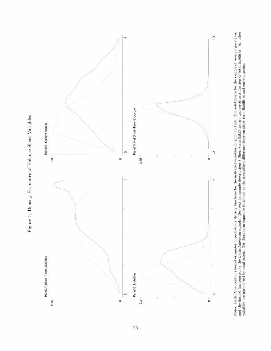
Several of the pertinent contrasts—and similarities–between the East Asia and Latin America are

evident in Figure 1. This figure displays kernel estimates of the probability density functions of

four variables central to the present study: the fraction of liabilities due in the upcoming year,

1Appendix Table 1 reports these robustness tests in detail. We also regress a binary indicator for these corporateevents on the specifications used below, and do not find that our interaction variable of interest predicts having anevent.

6

the fraction of assets that are “current”, the ratio of liabilities to assets, and the net short-term

exposure. The density estimates for the Asia sample are represented by a solid line, and the

estimates for Latin America are displayed as a dashed line.

The density estimates for debt maturity and overall leverage confirm the conventional wisdom

about the balance-sheet deficiencies of East Asian corporations. In Panel A of Figure 1, we graph

the ratio of short-term to total liabilities. We see a marked difference between the regions on this

measure. While the Latin American distribution is roughly bell shaped and centered around six

tenths, the East Asia is shifted to the right (i.e., shorter term). Indeed, the mode of the Asia

density is almost at one (100% short term). Similarly, East Asian corporations tended to have

substantially greater liabilities than their Latin American counterparts, as seen in Panel C.

However, when we combine this with the other side of the balance sheet, the Asian situation

seems less dire. Of note in Panel B of Figure 1 is that the distribution of current (i.e., short term)

assets for East Asian corporates was also shifted to the short end, relative to Latin American firms.

To assess maturity structure on both sides of the balance sheet, we take the difference between

short-term liabilities and current assets, which we call short-term exposure. The regional density

estimates of this difference are displayed in Panel D. The Asia distribution does not exhibit the

rightward shifting seen in the case of short-term liabilities. Indeed, the densities from both regions

align very closely.

The regional similarity in the distribution hardly dispels preoccupations about the risk of short-

term exposure. Credit markets in either region may not be robust enough to transfer capital from

the lower to the upper tail (of Panel D) in a crisis. Moreover, this could be exacerbated for Asia

by the fact the distribution of short-term exposure is a bit more spread out than in Latin America.

On the other hand, the shocks to capital markets in East Asian may have placed a greater penalty

on short-term exposure. With these uncertainties in mind, we set out to measure the effects of

short-term exposure below.

III Investment Regressions

In this section, we examine the “maturity mismatch” hypothesis and find it lacking. We fail to find

robust differences in the investment behavior among firms with very different levels of potential

exposure to the flight of capital from the country. Specifically, we propose and implement a simple

regression equation that allows for the estimation of differential responses to capital flows by firms

7

with different maturity structures on their balance sheet. In almost every case, we find that this

relationship is not significantly different from zero, and in no case do we find a robustly significant

effect.

III.A Empirical Methodology

The central empirical question of this study is how the change in domestic credit interacts with

the maturity structure of firms’ balance sheet to alter investment behavior. Therefore, the key

explanatory variable in the analysis is the interaction of firm i’s lagged short-term exposure, expSTi,t−1,

with aggregate (net) capital flows, ∆kjt, into country j at time t . (In what follows, we abbreviate

this second-order term as (expST × ∆k) for brevity.) The prediction of the maturity-mismatch

hypothesis is that firms with more short-term debt should invest less following an episode of capital

flight. Since an outflow is defined negatively, this implies a strongly positive coefficient on (expST ×

∆k). (The exception being for the disposal of capital, for which we expect a negative relationship.)

In addition to the interaction, we include terms that control for the first-order effects of balance-

sheet variables and macro conditions. Including the main effect of short-term debt absorbs any pre-

existing differences among firms with different levels of short-term indebtedness. Such differences

might have prevailed in the absence of movements in the capital account, e.g., if expanding firms

were more likely to issue short-term debt than stagnant ones. (Below, we refer to lagged short-

debt exposure mnemonically as expST .) The macro main effect, a fixed effect for country × year,

captures the macroeconomic changes that may impact all firms in the economy without regard to

the maturity composition of their balance sheet.

The basic specification (for firm i in country j at year t) that results is

Iijt = β(expSTi,t−1 ×∆kt) + δjt + γexpST

i,t−1 + εijt (1)

in which Iijt is a measure of investment. We estimate this equation using Ordinary Least Squares

(OLS) on the accounting data described above. Note that investment is therefore modeled as

a function of predetermined micro-level variables plus the contemporaneous (macro) measure of

capital flows, which is exogenous to any particular firm. Therefore, OLS can consistently estimate

this reduced-form equation. To equation 1, we also add additional firm and macroeconomic control

variables. For example, we typically include a control for lagged total debt and current assets, as

well as their interactions with the capital flow. Other examples are detailed below.

8

III.B Results for Whole Sample

Among firms in our sample, we find no robust, statistically significant evidence that short-term

exposure reduced investment following capital flight. We employ the empirical methodology detailed

above, and pay particular attention to the estimated coefficient on the interaction of lagged short-

term debt and capital flows, (expST×∆k). We generally estimate this coefficient to be insignificantly

different from zero: i.e., approximately the same response of investment by “short-term” and “long-

term” firms to aggregate capital flows.

This result can be seen in Table 3, which contains estimates of equation (1) and variants.

Columns (1), (4), (7), and (10) show the estimate of the simplest equation, a specification that con-

sists exclusively of (expST ×∆k), the first-order effect of lagged short-term debt, and country×year

fixed effects. Columns (2), (5), (8), and (11) add leverage and current assets as controls and as

interactions with the capital flows. Finally, in Columns (3), (6), (9), and (12), the specification

also includes a lagged dependent variable as an independent regressor. The inclusion of the lagged

dependent variable allows for the presence of adjustment costs. We estimate the effect on current-

year investment in Panel A, whereas Panel B contains results for investment for the following year

as the dependent variable. (Note that all the micro-level variables are lagged one year, so “current

year” means contemporaneous with the macro variable. For Panel B, the dependent variable is

from period t + 1 and the lagged dependent variable is therefore from period t.) We review the

results for each type of investment in turn in the following paragraphs.

First, the interaction of short-exposure and capital flows is not a robust determinant of capital

expenditures. The basic result for capital expenditures are the most favorable to the maturity-

mismatch hypothesis. In Column (1), we see that the OLS estimation of equation (1) without

additional controls yields a positive and significant coefficient on (expST × ∆k). However, this is

not robust to the inclusion of additional balance sheet data or of the lagged dependent variable. We

also estimate a positive correlation between short-term exposure and investment in Column (1).

When total debt and its capital-flow interaction are both added to the regression (shown in Column

(2)), the first-order effect of expST is no longer significant.

Second, (expST × ∆k) is not a robust, correctly signed determinant of the disposal of fixed

assets. The more parsimonious specifications yield significant, positive estimates of the effect of

(expST × ∆k) on asset sales. However, this effect is weaker upon inclusion of a lagged dependent

variable. In any case, since we expect more asset disposal by short-term-exposed firms when the

9

capital account is negative, the initial results have the apparently incorrect sign. This raises a

possible limitation of the accounting data: sales of assets measure price × quantity. If financially

distressed are forced into holding “fire sales” of their assets, the response of price might exceed

the response of quantity. To be sure that our results are not contaminated by price effect, we also

examine the extensive margin of disposal.2 These results are located in Columns (7) through (9)

of Table 3. We find no robust and significant effect of (expST ×∆k) on the probability that a firm

sells fixed assets.

Third, the coefficient on (expST ×∆k) is insignificantly different from zero in all specifications

for inventory investment. This result is peculiar since the inability to renew short-term debt should

restrict firms’ working capital particularly. Firms apparently do not run down inventories in order

to make up this gap. On the other hand, the interaction of current assets with capital flows is

estimated to be significant, but with a puzzling sign (more liquid assets should be good in the face

of capital flight).

These tests most likely do not suffer from a lack of statistical power due to noisy firm data. One

could argue that poor accounting standards introduce substantial noise into these measures. On the

other hand, a common argument is that poor standards introduce not noise, but systematic biases

such as exaggeration of profits. Either way, it is clear from the results that accounting variables, in

first-order form, are significant predictors of the various investment variables. This indicates that

the data are not so error prone. It is only when we look for interactions of short-term exposure

with macro shocks that we generally do not find significant effects.

III.C Regional Comparisons

The non-effect of short-term exposure from above is seen in our regional analysis as well. Table 4

contains regression results for each region and for each investment variable. The regression speci-

fication is as in Column (3) of Table 3, with a lagged dependent variable and with total liabilities

and current assets entering in first-order form and as interactions with the net capital account. In

no case do we estimate a significant (and correctly signed) effect of (expST ×∆k) on investment.

Regional differences do emerge on some of the other interactions. Using the samples from Latin

America and from the additional emerging markets, we estimate all of interaction effects to be

insignificantly different from zero for current investment. On the other hand, several interaction

2Approximately fifty percent of the firm/year observations are characterized by some sales of fixed assets.

10

terms are estimated to be significantly different from zero for the East Asian sample. The interaction

of current assets with capital flows has roughly equal and opposite effects on capital expenditures

and inventory investment. While the net effect is a statistical zero, it is noteworthy that some sort

of shifting is apparently induced by (expST ×∆k). We also estimate a significant, positive effect of

the interaction between liabilities and capital flows for several types of investment, which suggests

that firms with higher leverage in East Asia were more vulnerable to capital flight.

IV Sensitivity Analysis

The result from above is not sensitive to a wide variety of changes in the econometric specification,

as we show in this section. These alternative specifications include using different estimators and

alternative measures of capital flows. Further, we show that the result for (expST × ∆k) is robust

to the inclusion of control variables for access to external capital and changing relative prices.

IV.A Alternative Estimators

We estimate the effect of (expST ×∆k) using numerous alternative estimators, all of which deliver

similar estimates of (expST × ∆k) to those above. These new results are seen in Table 5 and

described in this subsection.

We begin with alternative computations for the standard errors using the ordinary least-squares

(OLS) estimator. These estimates employ the specification from Table 3, Column 2, which includes

first-order and capital-flow-interaction effects of short-term exposure, total liabilities, and current

assets. Each Panel displays only the estimates on (expST × ∆k). (Note that the point estimates

do not change in Panels A-D, only the standard errors.) Panel A contains the basic OLS stan-

dard errors, i.e., assuming no heteroskedasticity and no intraclass correlation. Panel B reports

Huber-White (“robust”) standard errors that allow for heteroskedasticity. (These are the default

throughout the present study.) Panel C allows for corrects the errors for the presence of correlated

disturbances across firms within each country × year cell. Finally, in computing the standard errors,

the estimator in Panel D allows for fairly generic correlational structures within firm. The size of

the standard errors generally increases as we read down the Panels, but the pattern of significance

is essentially the same.

These results are essentially unchanged if we add a one-period lag of the dependent variable.

These estimates of the effect of (expST × ∆k) are shown in Panel E (which replicates parts of

11

Table 3). This provides a useful check for the above estimates insofar as firms experience persistent

shocks.

When we control more flexibly for the predetermined variables, very little changes in our es-

timates. Above, we use linear terms to control for the first-order effects of the lagged accounting

variable (expST , total debt and current assets). In Panel F, we allow the effects of the predeter-

mined accounting variables (short-term exposure, total debt, current assets) to be highly flexible

by including them as polynomial of order ten. In effect, we are parametrically matching firms based

on their t − 1 characteristics. The estimates are qualitatively similar using this technique, with

the major exception that the anomalous result for the disposal (sale) of fixed assets is no longer

significantly different from zero.

Controlling for firm-level fixed effects does not generate estimates that favor the maturity-

mismatch hypothesis. In Panel G, we add firm-specific effects to the specifications. Similar esti-

mates are obtained, except for the contemporaneous response of capital expenditures to (expST ×

∆k) (for which the estimate is significant but opposite of the excepted sign). We combine the

matching estimator with firm fixed effects in Panel H, and find uniformly insignificant effects of

(expST ×∆k) on all the studied investment outcomes. This includes an insignificant result for ex-

penditures (versus Panel G, Column 1) and for disposal (versus the majority of the Panels above).

Finally, the addition of an autocorrelated error term yields substantially similar results. We

allow for an autoregressive error of order one (AR(1)) at the firm level in the estimation of the

fixed-effects model. These results are found in Panel I. The estimated standard errors tend to be

larger than those found above, and the point estimates are similar. Consequently, none of the

estimates of (expST ×∆k) are significantly different from zero.

IV.B Alternative Normalizations

Above we normalized the accounting variables by lagged total assets, but we obtain similar results

for (expST ×∆k) with alternative normalization schemes. These new estimates are found in Table 6.

Panel A repeats the baseline estimates from above. In Panel B, we consider a broader measure

of (lagged) firm value: outstanding debt plus market capitalization. In Panel C, we normalize

instead by the lagged capital stock (or stock of inventories in the case of inventory investment). In

Panels D and E, we scale the independent variables by lagged assets and firm value, respectively, but

12

normalize the investment variables with the lagged stocks as above.3 In no instance do we estimate

an effect of (expST ×∆k) that is consistent with the maturity-mismatch hypothesis. Renormalizing

the investment variables by lagged capital stocks does render insignificant, in most instances, the

interactions of the net capital account with current assets.4

IV.C Alternative Measures of Capital Flows

In this subsection, we estimate the effect of (expST ×∆k) using interactions of exposure with various

alternative macroeconomic variables.

We start by looking at the differential effects on firm level investment of capital inflows net of

foreign direct investment (FDI). We exclude foreign direct investment to control for the possibility

that “fire sale FDI” takes place during a balance of payment crisis. So far we have associated an

international liquidity shock with low foreign investment and the exiting of investors from the crisis

economy. However, a liquidity crisis could also consistent with an inflow of foreign capital, in the

form of mergers and acquisitions (M&A), that seeks to take advantage of profitable investment

opportunities in the hands of cash-strapped domestic corporations5. We report these results in

Panel B of Table 7. As in our baseline specification, we fail to find a significant differential effect

of short-term exposure on the response of investment to capital flows.

Many of the capital-flow reversals in our sample coincide with periods of high domestic interest

rates, a result of dogged defenses of the exchange rate by domestic monetary authorities. The result

is that firms wishing to roll-over short term liabilities are restricted by the lack of both international

and domestic liquidity. To capture this effect we introduce a measure of shocks to the supply of

domestic credit in our investment specifications. Because data on interest rates is patchy, and has

the added complication of having to separate real rates from expected inflation, we proxy local

credit conditions using the change in domestic credit over lagged GDP. We start by estimating our

baseline specification and replacing net capital inflows with changes in credit. The results of this

estimation are reported in Panel C. Next, in Panel D, we include both the interaction of exposure

with capital inflows and changes in private credit. In all cases we fail to obtain coefficient estimates

3We also reproduce these specifications, but re-weight the data by the lagged fixed-capital or inventory stock, asappropriate. Results are similar.

4We also replicated Table 6 using the “exposure only” specification seen in Columns 1, 4, 7 and 10 of Table 3.The significant estimates of (expST ×∆k) in those columns disappear when the lagged stock is used to normalize theaccounting variables.

5Aguiar and Gopinath (2002) find that there was a substantial increase in M&A activity in South East Asiabetween 1996 and 1998. See also Krugman (1998).

13

on the (expST ×∆k) interaction that are statistically significant.

As an additional test of the robustness of our main results, we repeat the specifications reported

in the previous three panels normalizing the measures of capital flows and changes in private credit

to zero mean and unit standard deviation by country. The results (reported in Panels E through

G of Table 7) are qualitatively identical to the results presented in Panels A though C.

Finally, in Panels H and I we report the estimated coefficients on the interaction between

exposure and the spread over US T-Bills of the JP Morgan EMBI bond index. Panel H uses the

country specific spread (when available), while Panel I uses the aggregate EMBI spread, which

should be taken a proxy of financing conditions for emerging markets in general. In both cases

the sample size drops: in the first case because EMBI data is only available for a sub-sample of

countries, in the second because data is only available after 1991. Consistent with our previous

results, we fail to find a significant negative coefficient on any of the interactions between exposure

and either of the EMBI spreads.

Could it be that the relationship between capital inflows and short-term exposure is non-linear,

so that it is only in periods of low inflows (or capital-flow reversals) that exposed firms fare worse

than their counterparts? We explore this question in the rest of Table 7.

We start with an indicator variable for periods in which capital inflows are below the country

median over the period 1985–2002 (low inflows). In Panel J we interact this indicator variable with

short term exposure, while in Panel K we interact the indicator variable with (expST × ∆k), thus

allowing for an asymmetrical effect of capital inflows. The next two panels replicate this exercise,

but define the indicator dummy with respect to the country mean minus one standard deviation

(crisis inflows). For most investment variables (current and next period) we obtain statistically

insignificant coefficients for the interactions of short term exposure with the dummy variables and

for the two interactions of exposure with net capital inflows. One exception are the capital disposal

variables, which display the familiar anomalous coefficients, although these anomalies seem to

obtain in periods of inflows in the interactive models.

Next, we consider investment behavior around particular episodes of capital-account reversals

and fail to find a significant effect of short-term exposure following capital flight. These episodes

are enumerated in Table 8. Table 9 shows the result of estimating the differential effects of the

Calvo et al (2004) measure of sudden stops. Instead of pooling the whole sample, we concentrate

on the fall in investment in the vicinity of the sudden-stop episodes. To do so we run a series of

14

regressions in which we include observations on firm investment from t− 1 (the period prior to the

sudden stop) and either t, t + 1 or t + 2. Note that each regression has observations from only two

periods. The key variable in this specification is the interaction between the post dummy (which

takes on a value of one in t, t + 1 or t + 2) and short term exposure. For this specification, we

expect a negative coefficient estimate on ((expST ) × Post) in the capital-expenditure and inventory

regressions, and positive signs in the asset-disposal equations. The odd-numbered columns report

estimates of specifications with expST , (expST × ∆k), and Post only, while the even-numbered

columns also include interactions between the post dummy and lagged liabilities and between the

post dummy and lagged current assets.

We find that, following a sudden stop, the behavior of capital expenditures in firms with high

exposure is, in almost all cases, statistically indistinguishable from the behavior of firms with low

exposure (columns 1–6). This result holds for the full sample, for sudden stop episodes in Asia

and for those in Latin America. The only (expST× Post) coefficient that is statistically significant

in both specifications is that for period t + 2 in Latin America, however, the estimated coefficient

is the opposite sign to what we expected. In turn, for inventory investment, disposal of fixed

assets and the disposal dummy, either the coefficients on (expST× Post) become insignificant once

the additional controls are included, or the estimated coefficients have opposite signs to what we

expected.

All in all the results presented in this subsection confirm our main results: we fail to find

significant, robust differences in the response of investment to international liquidity shocks across

firms with different levels of short-term exposure.

IV.D Additional Controls

Even though episodes of capital flight are times in which relative prices change markedly, we argue

that this is unlikely to contaminate our results. To a first approximation, this should load onto the

macroeconomic variables (not the interaction terms) since all the firms in the economy face these

same price changes. On the other hand, firms with more expST might face differential changes in

prices, a hypothesis we consider (and discard) in this subsection.

One possibility arises because changing credit-market conditions presumably have effects that

work through channels other than expST . If short-term-exposed firms also have differential access to

international (or domestic) capital, then our results may come from having omitted this “access”

15

variable in the estimates of investment responses to capital flows. We assess this hypothesis in

Table 10 by constructing proxies for capital access and controlling for them (interacted with ∆k)

in the investment regressions. In Panel A, we interact whether the firm had an ADR account in

year t− 1 with subsequent capital flows. There is mixed evidence on the effect of this interaction,

but its inclusion does not materially alter the estimates of (expST × ∆k). Similarly in Panels B

and C, respectively, we control for the firm having an active listing in the local stock market, or a

cross listing elsewhere. Again, the crucial new control is the interaction of these dummies with the

capital account. As with the ADRs, when we include these controls the estimates of (expST ×∆k)

change very little. A credit crunch might also have a greater impact on smaller firms. However, the

inclusion of controls for firm size hardly changes the result for (expST × ∆k), as seen in Panel D.

An interesting additional result is that small firms appear to be more vulnerable to capital flight.

Finally, we include interactions of industry (SIC1) dummies with the net capital account. As seen

in Panel E, we obtain similar estimates of the effect of short-term exposure when including these

additional controls.

Another possibility is that short-term and long-term-indebted firms systematically different in

the exchange-rate sensitivity of their non-financial prices, perhaps because of differing propensities

across sectors to issue short-term debt. Since the capital account and the exchange rate often move

together, there is potentially an omitted variable: the change in profit opportunities resulting from

the exchange-rate movement. We consider this hypothesis in Table 11. As a first approximation for

measuring changing profit opportunities we include earnings (measured by EBITDA) in our baseline

specification. Second, in Panel B, we include the interactions of exposure, current assets and total

liabilities with changes in the real exchange rate. Next, Panel C, includes interactions between

changes in the real exchange rate and 1 digit SIC dummies, while Panel D includes interactions

between a dummy for exporting firms and the change in the real exchange rate. Finally, Panel E

combines these last two sets of interactions in one specification. Moreover, we also find that detailed

time-varying sectoral controls6 (Panel F), which do not substantially affect the coefficient estimate

on (expST ×∆k) either.

Similarly, the short-term exposure of the firm could be correlated with its currency composition

of debt, because of so called “original sin” (Eichengreen and Hausmann, 1999). According to this

view, firms in emerging markets can either borrow short term or in a foreign currency. This being

6These include indicators for country × year × SIC1.

16

the case, firms face a tradeoff between currency risk and interest-rate/rollover risk. It should be

noted that we do not know the currency composition of the debt, so we cannot directly test for the

importance of the interaction of foreign-currency debt (D∗) with the exchange rate (∆e). Instead,

our approach is to add the interaction (expSTi,t−1 × ∆ejt) to the regression. Note that we do not

promote this variable as the definitive proxy for currency-mismatch effects. What we argue is that

it serves to determine whether the earlier estimates are contaminated by the suggested omitted-

variable bias.7 As seen in Panel B of Table 11, the inclusion of interactions among the debt variables

and ∆e does not yield substantially different estimates of the effect of (expST ×∆k). On the other

hand, the question of the interaction of maturity and currency mismatches during a crisis is explored

directly by Bleakley (2003). In a sample of Latin American firms, he finds a negative correlation

between short-term and foreign-currency debt. However, the omission of currency composition of

debt is found not to affect the conclusions regarding the effects of short-term exposure.

Belonging to business groups and conglomerates (such as the chaebol in Korea or grupos in

Mexico) provides access to an internal capital market, which may distort the choice of debt maturity

and confound the effect of this debt in periods of capital outflow. To assess how this affects our

estimates of (expST × ∆k), we assemble additional information on the ownership characteristics

of the corporations in our sample.8 For the Latin American subsample, we use the Corporate

Affiliations database (Lexis-Nexis, 2003) to measure ownership characteristics. The first category,

labelled “subsidiary” in the Table, denotes subsidiaries or joint ventures. A second category is

created for affiliates, and a third for corporations with diluted ownership. The omitted category

is for those firms that do not appear in the Corporate Affiliations database. In the East Asian

subsample, we use the classification scheme for ownership described by Claessens, Djankov, and

Lang (2000).9 The first category is for those corporations that are widely held, i.e. that do not have

significant concentration of ownership. We create three additional categories for firms affiliated with

banks, families, and governments. Finally, the omitted category is for those firms left unclassified

7Consider two cases. First, suppose that corr(D∗ijt−1, expST

i,t−1) = α 6= 0. Upon inclusion of expSTi,t−1 ×∆ejt in the

regression, the component of D∗ijt ×∆ejt that is not correlated with expST

i,t−1 ×∆ejt remains in the error, but doesnot cause a bias in the coefficient on (expST

i,t−1 ×∆kt). On the other hand, suppose that corr(D∗ijt−1, expST

i,t−1) = 0.In this case, there is no omitted variable bias to begin with, although including this measure might improve theprecision of the estimates. In either case, adding (expST

i,t−1 × ∆ejt) corrects any omitted-variable bias arising from

the correlations among{D∗, expST

}. But note that (expST

i,t−1 ×∆ejt) need not be correlated for (D∗ijt ×∆ejt) for

this test to be informative.8It should be noted that these variables are from a single point in time. In East Asian, information is from 1996,

while in Latin America it is from 2003.9We thank Todd Mitton for providing with these data.

17

by Claessens et al.. For both regions, the categories are mutually exclusive.

Controlling for affiliations does not affect our main result for maturity mismatch. In Table 12, we

include these ownership indicators in the regression, interacted with the capital account. Because

the data are different by region, we run the analysis separately for Latin America and East Asia.

In Panels A and C, we present the baseline results for (expST ×∆k). In Panels B and D, we show

results from regressions that allow for different sensitivities to the capital account across ownership

classes. While there is some evidence that corporations with group affiliations respond differently

to the capital account, the inclusion of these controls does not significantly affect our estimates of

(expST ×∆k).

V Effect on the Net Worth

We discuss the response of financial and income variables to (expST × ∆k) in this Section. A

plausible explanation for the results might have been that firms had successfully managed the risks

associated with short-term exposure through financial derivatives, perhaps. What we show in this

Section contradicts this notion. Short-term-exposed firms incur higher debt and interest obligations

going forward. There is also evidence of liquidation of assets at bargain prices In all, we estimate

a substantial transfer of wealth out of firms with more expST .

V.A Financing Variables

On average, short-term-exposed firms see their financial positions deteriorate with a capital outflow.

This is consistent with the maturity-mismatch hypothesis in that more short-term exposure means

more exposure to interest-rate shocks. We also find that the short-term-exposed firms did not choose

(or were unable) to repay their obligations that came due during the capital outflow. Instead, they

absorbed the shock by taking on higher interest and debt obligations.

The results for the full sample are found in Table 13. In the current year (i.e., contemporane-

ous with the capital account), there is evidence of significant effects of (expST × ∆k) on interest

payments, but less robust evidence of an effect on total debt or new issuances of debt. In the year

following the aggregate capital flow, we estimate a strong relationship between (expST × ∆k) and

total debt. In other words, short-term-exposed firms saw significant increases in their indebtedness

in the aftermath of a capital outflow from the home country. We also estimate statistically signifi-

cant reductions in the gross issuance of new debt among short-term exposure firms following capital

18

outflows, but at the same time less debt is retired, and as a result there is no effect of (expST ×∆k)

on net issuances.

V.B Income Statement

In this subsection, we address the effects of short-term exposure on firm income. We find that during

capital outflows firms with higher short-term exposure experience a larger drop in non-operating

income. Part of this is mechanical, and operates via higher interest rate expenses. Another part,

however is due to fall in non-interest components of the non-operating income. Evidence from a

sub-sample of firms for which data is available suggests that part of the fall is due to losses stemming

from asset sales. Firms with higher short term exposure are forced to hold a “fire sale” of assets in

order to deal with liquidity problems.

The results for the full sample are reported in panel A of Table 14. Each cell of the table

reports the estimated coefficient on the (expST × ∆k) interaction for a regression in which the

dependent variable is a component of the income statement. In the first row, the dependent

variable is operating income, i.e., that income which is directly related to the firm’s main line of

operation. As reported, we fail to find a positive coefficient on the (expST × ∆k) interaction for

either contemporary or period-t + 1 operating income. Where we do find a positive and significant

coefficient is for period-t non-operating income: firms with higher short-term exposure see a larger

deterioration in this category of income following a capital outflow. The next three rows report

results for different components of non-operating income. The first is income from interest bearing

assets or equity holdings of non-subsidiaries. We find no differential response to an outflow across

different levels of exposure for this variable. The second is accrued interest expenses. As discussed

in the previous subsection, firms with more short-term debt are more exposed to volatile interest

rates. The result is higher interest costs in periods of outflows. The third category is a broad income

category that includes, amongst other things, losses from sale of assets. We obtain a positive and

significant coefficient on the (expST ×∆k)interaction for this category of income.

To determine what may be driving the positive result for the other-non-operating-income cat-

egory, we repeat our estimation for the sub-sample of firms for which data on the loss from sale

of assets is available. This component of the income statement measures differences between the

accounting value of assets and the price at which they were sold. The estimated coefficient indicates

that firms with higher short-term exposure experience higher losses due to asset sales in periods

19

of outflows, and that in the sub-sample, approximately 25% of the period t effect of exposure on

other-non-operating-income is due to these losses. As our previous results for total value of liquida-

tion failed to find a negative differential effect, we interpret this result as evidence of higher losses

per unit sold. Firms with higher exposure are more likely to “fire-sell” their assets in periods of

capital-flow reversal.

The last two rows of panel A report the estimated coefficients on (expST ×∆k) when measures

of cash flow replace income as the dependent variable. The results are in line with the income

statement results: we find a non significant coefficient on the (expST × ∆k) interaction for cash

flow from operations but a positive and significant coefficient for earnings before interest, taxes,

depreciation and amortization (EBITDA).

VI Discussion of Average Investment

In this section we explore, and discard, two alternative hypotheses for our lack of results. The first

alternative explanation for the lack of a differential response to capital outflows across short term

exposure is that the variance of our LHS variables collapses to zero around these episodes. Simply

put, if all firms invest zero, then it will be impossible to find differences across categories. Although

the significant coefficients on many interaction variables in previous specifications suggest that this

is not the case, we explore this hypothesis in this section directly by looking at the dispersion of

investment around episodes of capital flow reversal. The second explanation is that our sample of

firms is not representative, so that the large collapse in investment observed during these “crises”

occurs only elsewhere in the economy, specifically in small unlisted firms. We find that this is not

the case. Indeed, as shown below, the elsaticity of aggregate investment in our sample to capital

flows is remarkably similar in magnitued to the elasticity of private gross fixed capital formation

as reported by national accounts.

VI.A Changes in the Distribution of Investment

In Figure 2, we see how the cross-firm distribution of investment changed during the crisis episodes

that qualified as “sudden stops”10. Panel A contains estimates of the probability density function

of investment (defined as the sum of all investment components above), while Panel B plots the

10These episodes are specified in Table 8.

20

time path of the first and second moments. In the notation of the Figure, a crisis starts in year t.

The distribution of investment is quite similar in years t − 1 and t − 2. In the year of the sudden

stop (i.e., year t), the investment distribution shifts somewhat to the left, and is slightly more

dispersed. Going forward, investment is dramatically lower and the distribution is tighter around

the mean in years t + 1 and t + 2. In this time span, average investment declines by more than

50%, while the standard deviation drops by around 15%.

In light of this evidence, can the results from Section III be explained as being because “no

one was investing anyway” in these episodes?11 We suggest that they cannot. First, dispersion

of investment actually rises in the year in which the sudden stop in capital flows (and corporate

investment) begins. Second, while the cross-firm dispersion in investment is lower in the two years

following the crises, the standard deviation is only lower by some fifteen percent of the starting

value.

VI.B Corporate versus Aggregate Response

While the focus of the present study is the corporate sector, it is worth considering how the full

economy’s investment responds to capital flight. Large, publicly traded firms generally have better

access to external capital, and it is natural to wonder whether this advantage helps them endure the

credit-market shocks better than the small and medium enterprises in the same economy. More-

over, if, in the face of these shocks, the large corporations turn to domestic sources of credit, their

retrenchment might displace the smaller firms. On the other hand, it is precisely the large corpo-

rations that are more exposed to international shocks because they are more likely to participate

in international capital markets.

We construct comparable measures of investment for both our sample and the broader economy.

We focus on purchases of equipment and structures, which correspondes to fixed-capital purchases

from the cash-flow statement in our sample and to gross fixed-capital formation in the national

accounts (and in the WEO). Because the strategy from above of normalizing by lagged assets is not

feasible for the aggregate data, we consider yearly logarithmic changes in the CPI-deflated levels

of investment, and thereby construct a time series of growth rates for each country represented in

our sample.

We regress these two investment variables on capital flows for the panel of countries in our

11We are grateful to Peter Garber for suggesting this as a possible explanation for our results.

21

data. These results are found in Table 15. In Panel A, the dependent variable is the fixed-capital

investment of the entire private sector. In Panel B, capital expenditures from our sample of publicly

traded firms are on the left-hand side.12 These resulting estimates are of similar magnitude (not

simply the same sign) for the two series. The major systematic difference that emerges is that the

corporate sector tends to have a stronger contemporaneous response to the capital account, while

the broader private sector has a larger response in the following year. This is consistent with the

smaller firms being exposed to international shocks, with a delay, through the banking system.

Nevertheless, the total effect over time of the capital account is similar across sectors.

VII Conclusions

Using micro data from emerging-market corporations, we examine the response of investment to

aggregate capital flows. We do not find robust and statistically significant differences in the in-

vestment response among firms with very different levels of potential exposure to the flight of

capital from the country. This evidence casts doubt on the importance of corporate-level maturity

mismatch in these countries.

We obtain a series of additional results that we believe merit further research. First, we find that

some categories of firms do experience large drops in investment during capital-account reversals.

This is the case of highly leveraged firms in East Asia, and the smaller firms throughout our

sample. Second, we find that short-term exposure does have effects on firm outcomes. In periods of

capital outflows those firms in our sample with higher exposure: accumulate more debt, incur higher

interest costs, have lower non-operational income, and sell-off assets with larger mark-downs. Many

of these results suggest important transfers of wealth within the economy (and potential across

borders as well). We also find that firm with higher exposure are less likely to access new debt

financing following a slow down in capital inflows, suggestting they are forced to obtain financing

for their production and investment elsewhere, be it internal or by seeking external sources of equity

financing.

12While the latter series is a component of the former, it does not represent more than twenty percent of investmentin the private sector in any country we study.

22

References

Aguiar, M. and G. Gopinath, G. (2002). “Fire-Sale FDI and Liquidity Crises”. Mimeo, Universityof Chicago.Bleakley, H. (2003). “Descalce de plazos y crisis financiera: evidencias en las empresas de AmericaLatina.” Perspectivas: Analisis de temas crıticos para el desarrollo sostenible, December 2003,1(2):9-28.Calvo, G. A., A. Izquierdo and L. Mejia. (2004). “On the Empirics of Sudden Stops: The Relevanceof Balance-Sheet Effects.” NBER Working Paper No. 10520.Cowan, K. and J. de Gregorio (1998). “Exchange Rate Policies and Capital Account Management:Chile in the 1990s.” In Glick, R. (ed.), Managing capital flows and exchange rates: Perspectivesfrom the Pacific Basin. Cambridge; New York and Melbourne, Cambridge University Press: 322-55.Chang, R. and A. Velasco (1999). “Illiquidity and Crises in Emerging Markets: Theory and Policy.”NBER Macroeconomics Annual, 1999.Claessens, S., S. Djankov and L. Lang (2000). “The separation of ownership and control in EastAsian Corporations.” Journal of Financial Economics 58: 81-112.Detrgiache, E. and A. Spilimbergo (2002). “Empirical Models of Short-Term Debt and Crises: DoThey Test the Creditor-Run Hypothesis?” Mimeo, International Monetary Fund, May.Diamond, D. W. and P. H. Dybvig (1983). “Bank Runs, Deposit Insurance, and Liquidity.” Journalof Political Economy 91(3): 401-19.Eichengreen, B. and R. Hausmann (1999). “Exchange Rates and Financial Fragility.” NBERWorking Paper 7418.Everhart S. and M. Sumlinski (2001). “Trends in Private Investment in Developing CountriesStatistics for 1970-2000 and the Impact on Private Investment of Corruption and the Quality ofPublic Investment”. IFC discussion Paper 44. Data available online athttp://www.ifc.org/ifcext/economics.nsf/Content/DataSets.Fazzari, S. M., R. G. Hubbard and B. Petersen (1988). “Financing Constraints and CorporateInvestment.” Brookings Papers on Economic Activity 0(1): 141-95.Gallego, F. and N. Loayza (2000). “Financial Structure in Chile: Macroeconomic Developmentsand Microeconomic Effects.” Working Paper 75, Central Bank of Chile.Gelos, G. and A. M. Werner (1998). “La Inversion Fija en el Sector Manufacturero Mexicano 1985-94: El Rol de Los Factores Financieros y El Impacto de Liberalizacion Financiera.” Documento deInvestigacion No. 9805, Banco de Mexico.Hoshi, T., A. Kashyap and D. Sharfstein (1991). “Corporate Structure, Liquidity, and Investment:Evidence from Japanese Industrial Groups.” Quarterly Journal of Economics 106(1): 33-60.Hubbard, R. G. (1997). “Capital-Market Imperfections and Investment.” NBER Working Paper:6200.International Monetary Fund (2004a). International Financial Statistics. Electronic database,June 2004.— (2004b). World Economic Outlook Database. Electronic database.Lang, L., E. Ofek and R.M Stulz (1996). “Leverage, Investment, and Firm Growth.” Journal ofFinancial Economics 40(1): 3-29.Lexis-Nexis (2003). Corporate Affiliations Plus. Electronic database, June 2003.

23

Love, I. (2001). “Financial Development and Financing Constraints: International Evidence fromthe Structural Investment Model.” World Bank Working Paper 2694.McKinnon, R. I. and H. Pill (1998). “The Overborrowing Syndrome: Are East Asian EconomiesDifferent?” In R. Glick (ed.), Managing capital flows and exchange rates: Perspectives from thePacific Basin. Cambridge; New York and Melbourne, Cambridge University Press: 322-55.Radelet, S. and J. D. Sachs (1998). “The East Asian Financial Crisis: Diagnosis, Remedies,Prospects.” Brookings Papers on Economic Activity (1): 1-74.Thomson Financial (2003). Worldscope Database. Electronic database, May 2003.

24

Fig

ure

1:D

ensi

tyE

stim

ates

ofB

alan

ceSh

eet

Var

iabl

es

P

anel

A: S

hort−

Term

Lia

bilit

ies

0

1

0

2.15

Pan

el B

: Cur

rent

Ass

ets

0

1

0

2.3

Pan

el C

: Lia

bilit

ies

0

2

0

2.3

Pan

el D

: Net

Sho

rt−Te

rm E

xpos

ure

−1

1.4

0

3.15

Note

s:E

ach

Panel

conta

ins

ker

nel

estim

ate

sofpro

bability

den

sity

funct

ions

for

the

indic

ate

dvari

able

sfo

rpri

or

to1996.

The

solid

line

isfo

rth

esa

mple

ofA

sia

corp

ora

tions,

and

the

dash

edline

repre

sents

the

Latin

Am

eric

an

sam

ple

.(S

eete

xt

for

sam

ple

des

crip

tions.

)Short

-ter

mliabilitie

sare

expre

ssed

as

afr

act

ion

ofto

talliabilitie

s.A

lloth

ervari

able

sare

norm

alize

dby

tota

lass

ets.

Net

short

-ter

mex

posu

reis

defi

ned

as

the

norm

alize

ddiff

eren

cebet

wee

nsh

ort

-ter

mliabilitie

sand

curr

ent

ass

ets.

25

Figure 2: Changes in the Distribution of Investment Following A Sudden Stop

Panel A: Density Estimates

02

46

8

−.2 0 .2 .4 .6 .8Total Investment / Lagged Assets

t−2t−1tt+1t+2

Panel B: Time Series of Summary Statistics

.06

.08

.1.1

2.1

4.1

6

−2 −1 0 1 2Years, Relative to Sudden Stop

MeanStandard Deviation

Notes: Total investment is the sum of capital expenditures, (minus) disposal of fixed assets, and inventory investment. In-vestment is normalized by lagged assets. The sample is restricted to firms in those countries that experienced “Sudden Stop”episodes. (See text for further sample and variable descriptions.) Panel A contains estimates of probability density functionsin the years before, during, and after a sudden stop. Each curve is an estimate from a particular year (relative to episode),as indicated by the line style. The x-axis is total investment over lagged assets and the y-axis plots the estimated density.Panel B contains a plot of the movement of the mean and standard deviation of total investment around sudden-stop episodes.The x-axis is the number of years relative to the initial onset of the sudden stop, while the y-axis plots the indicated samplemoments for the indicated year.

26

Tab

le1:

Sam

ple

Cov

erag

e

.Y

ear o

f Obs

erva

tion

1981

1982

1983

1984

1985

1986

1987

1988

1989

1990

1991

1992

1993

1994

1995

1996

1997

1998

1999

2000

2001

2002

Tot

als

for

Prin

cipa

l Loc

atio

n of

Fir

mal

l yea

rs:

Eas

t Asi

aIn

done

sia

27

6772

7779

103

115

120

122

114

182

101

1161

Sout

h K

orea

1618

2020

2223

1921

8011

310

410

711

817

220

422

626

128

035

364

669

835

438

75M

alay

sia

2628

2727

3338

3848

5460

6812

014

415

116

322

927

429

329

431

851

266

036

05Ph

ilipp

ines

44

722

3235

3759

6864

6368

112

4662

1T

haila

nd

2

413

2581

134

175

183

196

212

209

200

197

300

305

2236

Lat

in A

mer

ica

Arg

entin

a

3

99

99

1924

2830

3039

4257

7276

6852

4B

rasi

l

52

5660

5979

8287

103

134

135

148

172

320

311

173

1971

Chi

le

1

316

1922

2440

4249

5661

6771

9614

714

311

196

8C

olom

bia

1212

1310

1519

2122

2323

2222

2222

426

2M

exic

o17

2022

2227

2829

3333

3434

5063

6774

7578

8211

612

912

411

612

73Pe

ru

2

33

36

1722

1717

2829

3551

6043

336

Ven

ezue

la

1

13

36

89

910

1110

1723

195

135

Oth

er E

mer

ging

Mar

kets

Isra

el

22

2929

2632

4448

6288

5243

2T

urke

y

2

1019

2326

3141

4044

5574

9311

711

727

696

8So

uth

Afr

ica

7483

8198

115

129

127

131

128

144

149

154

152

168

357

390

341

1728

38

Tot

als

for a

ll co

untr

ies

5966

6969

156

173

173

296

400

484

503

769

936

1107

1195

1387

1550

1656

2045

2676

3105

2331

2120

5

Note

s:E

ach

cell

indic

ate

sth

enum

ber

of

firm

obse

rvations

conta

inin

gvalid

data

on

short

-ter

mex

posu

refo

rth

epre

vio

us

yea

rand

valid

capit

al-acc

ount

data

for

the

firm

’shom

eco

untr

y.

27

Table 2: Descriptive Statistics

Balance Sheet Variables Measures of Investment

(1) (2) (3) (4) (5) (6) (7)

Total Short-term Current Short-term Capital Change in DisposalLiabilities Liabilities Assets Exposure Expenditures Inventory of Fixed

(c2)-(c3) Stock AssetsCountries:

0.592 0.397 0.445 -0.048 0.077 0.005 0.008East Asia (0.357) (0.311) (0.200) (0.342) (0.119) (0.062) (0.023)

[11486] [11498] [11498] [11498] [10187] [10213] [9016]

0.590 0.395 0.473 -0.078 0.097 0.008 0.009 Indonesia (0.333) (0.317) (0.207) (0.372) (0.148) (0.073) (0.026)

[1161] [1161] [1161] [1161] [1042] [1038] [1031]

0.704 0.416 0.478 -0.062 0.071 0.007 0.011 South Korea (0.340) (0.219) (0.177) (0.251) (0.091) (0.054) (0.027)

[3870] [3875] [3875] [3875] [3332] [3454] [2489]

0.494 0.385 0.441 -0.056 0.070 0.004 0.008Malaysia (0.382) (0.370) (0.213) (0.388) (0.117) (0.067) (0.022)

[3603] [3605] [3605] [3605] [3270] [3229] [3052]

0.445 0.270 0.325 -0.054 0.105 0.001 0.005Philippines (0.281) (0.226) (0.197) (0.263) (0.185) (0.047) (0.022)

[621] [621] [621] [621] [604] [577] [552]

0.600 0.421 0.414 0.007 0.080 0.004 0.005Thailand (0.375) (0.357) (0.213) (0.396) (0.122) (0.063) (0.018)

[2231] [2236] [2236] [2236] [1939] [1915] [1892]

0.458 0.263 0.332 -0.069 0.074 0.005 0.005Latin America (0.279) (0.221) (0.189) (0.248) (0.099) (0.046) (0.020)

[5466] [5469] [5469] [5469] [4809] [4944] [3772]

0.439 0.279 0.341 -0.061 0.077 0.001 0.003Argentina (0.229) (0.208) (0.197) (0.264) (0.099) (0.049) (0.015)

[524] [524] [524] [524] [449] [466] [367]

0.518 0.308 0.333 -0.025 0.073 0.006 0.004Brazil (0.357) (0.278) (0.199) (0.303) (0.105) (0.047) (0.018)

[1968] [1971] [1971] [1971] [1742] [1842] [1350]

0.379 0.193 0.304 -0.112 0.087 0.006 0.009Chile (0.193) (0.128) (0.187) (0.161) (0.106) (0.034) (0.025)

[968] [968] [968] [968] [847] [830] [691]

0.392 0.216 0.316 -0.100 0.054 0.005 0.008Colombia (0.228) (0.166) (0.191) (0.127) (0.068) (0.048) (0.018)

[262] [262] [262] [262] [238] [251] [216]

0.465 0.250 0.346 -0.096 0.071 0.005 0.005Mexico (0.244) (0.209) (0.172) (0.234) (0.092) (0.049) (0.019)

[1273] [1273] [1273] [1273] [1106] [1122] [837]

0.439 0.292 0.362 -0.070 0.066 0.007 0.007Peru (0.241) (0.184) (0.186) (0.221) (0.105) (0.054) (0.024)

[336] [336] [336] [336] [302] [303] [207]

0.333 0.201 0.303 -0.102 0.054 -0.008 0.006Venezuela (0.153) (0.108) (0.161) (0.185) (0.061) (0.027) (0.024)

[135] [135] [135] [135] [125] [130] [104]

0.501 0.367 0.560 -0.193 0.108 0.002 0.008Other Emerging Markets: (0.241) (0.180) (0.220) (0.199) (0.134) (0.068) (0.022)

[5706] [5706] [5706] [5706] [5303] [5240] [3859]

0.443 0.267 0.542 -0.274 0.067 0.010 0.007Israel (0.209) (0.134) (0.240) (0.262) (0.059) (0.053) (0.018)

[432] [432] [432] [432] [390] [372] [309]

0.538 0.402 0.606 -0.204 0.133 -0.002 0.003Turkey (0.259) (0.178) (0.196) (0.188) (0.154) (0.071) (0.016)

[3097] [3097] [3097] [3097] [2804] [2773] [2047]

0.460 0.336 0.497 -0.161 0.082 0.005 0.015South Africa (0.219) (0.190) (0.246) (0.200) (0.114) (0.065) (0.028)

[2177] [2177] [2177] [2177] [2109] [2095] [1503]

Notes: Each cell contains a summary statistic for sampled firms in the indicated country or region. The top cell in each groupis the mean. The middle cell (in parenthesis) reports the standard deviation, and the bottom cell [in square brackets] indicatesthe number of observations. Variables (listed by column) are as described in the text. Short-term exposure in the differencebetween current liabilities and current assets. All variables are normalized by total assets.

28

Tab

le3:

Inve

stm

ent

and

Shor

t-Ter

mE

xpos

ure

(1)

(2)

(3)

(4)

(5)

(6)

(7)

(8)

(9)

(10)

(11)

(12)

Dep

ende

nt V

aria

bles

:

Inde

pend

ent V

aria

bles

Cap

ital E

xpen

ditu

res

Dis

posa

l of F

ixed

Ass

ets

Dis

posa

l of F

ixed

Ass

ets

> 0

Inve

ntor

y In

vest

men

tan

d R

egre

ssio

n St

atis

tics:

Pan

el A

: Dep

ende

nt V

aria

bles

from

the

Cur

rent

Yea

rIn

tera

ctio

ns w

ith C

apita

l Flo

ws:

Net

Sho

rt-T

erm

Exp

osur

e x

0.28

5 -0

.051

0.

014

0.04

5 0.

053

0.04

6 0.

197

-0.0

64

-0.0

42

-0.0

55

0.00

1 0.

035

Net

Cap

ital A

ccou

nt(0

.054

) ***

(0.1

06)

(0.0

93)

(0.0

14) *

**(0

.025

) **

(0.0

25) *

(0.1

75)

(0.3

87)

(0.3

46)

(0.0

33) *

(0.0

58)

(0.0

64)

Lev

erag

e x

0.13

2 0.

079

0.01

3 0.

004

0.39

6 0.

264

0.07

0 0.

076

Net

Cap

ital A

ccou

nt(0

.103

)(0

.084

)(0

.021

)(0

.022

)(0

.338

)(0

.304

)(0

.048

)(0

.054

)

Cur

rent

Ass

ets

x-0

.251

-0

.180

0.

023

0.02

4 -0

.140

-0

.060

0.

335

0.30

4 N

et C

apita

l Acc

ount

(0.1

09) *

*(0

.096

) *(0

.022

)(0

.024

)(0

.382

)(0

.350

)(0

.060

) ***

(0.0

64) *

**

Con

trol

s:

Net

Sho

rt-T

erm

Exp

osur

e0.

008

-0.0

04

0.00

9 0.

007

0.00

5 0.

004

0.01

2 0.

065

0.04

8 -0

.010

0.

001

-0.0

02

(0

.003

) **

(0.0

05)

(0.0

05)

(0.0

01) *

**(0

.002

) ***

(0.0

02) *

**(0

.010

)(0

.020

) ***

(0.0

18) *

**(0

.002

) ***

(0.0

03)

(0.0

04)

Lev

erag

e-0

.017

-0

.022

0.

004

0.00

3 -0

.045

-0

.049

-0

.012

-0

.011

(0.0

04) *

**(0

.004

) ***

(0.0

01) *

**(0

.001

) ***

(0.0

16) *

**(0

.013

) ***

(0.0

02) *

**(0

.003

) ***

Cur

rent

Ass

ets

-0.0

56

-0.0

15

0.00

2 0.

002

0.05

6 0.

066

0.00

1 -0

.003

(0.0

06) *

**(0

.006

) **

(0.0

01)

(0.0

01)

(0.0

20) *

**(0

.018

) ***

(0.0

03)

(0.0

04)

Lag

ged

Dep

ende

nt V

aria

ble

0.27

1 0.

183

0.38

4 -0

.065

(0

.024

) ***

(0.0

18) *

**(0

.007

) ***

(0.0

14) *

**

Reg

ress

ion

Stat

istic

s:

N

1765

317

643

1394

214

647

1463

911

608

2010

220

087

2002

317

915

1790

314

236

0.09

0.1

0.18

0.05

0.05

0.08

0.39

0.39

0.5

0.06

0.06

0.08

R2

Note

:Table

conti

nues

on

nex

tpage.

29

Tab

le3

(Con

tinu

ed):

Inve

stm

ent

and

Shor

t-Ter

mE

xpos

ure

(1)

(2)

(3)

(4)

(5)

(6)

(7)

(8)

(9)

(10)

(11)

(12)

Dep

ende

nt V

aria

bles

:

Inde

pend

ent V

aria

bles

Cap

ital E

xpen

ditu

res

Dis

posa

l of F

ixed

Ass

ets

Dis

posa

l of F

ixed

Ass

ets

> 0

Inve

ntor

y In

vest

men

tan

d R

egre

ssio

n St

atis

tics:

Pan

el B

: Dep

ende

nt V

aria

bles

from

the

Fol

low

ing

Year

Inte

ract

ions

with

Cap

ital F

low

s:

Net

Sho

rt-T

erm

Exp

osur

e x

0.40

1 0.

010

0.07

5 0.

030

0.04

4 0.

007

0.34

7 0.

261

0.30

2 -0

.041

-0

.031

-0

.039

N

et C

apita

l Acc

ount

(0.0

88) *

**(0

.162

)(0

.134

)(0

.012

) **

(0.0

26) *

(0.0

26)

(0.1

73) *

*(0

.379

)(0

.326

)(0

.037

)(0

.068

)(0

.072

)

Lev

erag

e x

0.22

0 0.

120

0.00

2 0.

017

0.18

4 -0

.003

0.

077

0.13

2 N

et C

apita

l Acc

ount

(0.1

68)

(0.1

06)

(0.0

22)

(0.0

22)

(0.3

24)

(0.2

80)

(0.0

62)

(0.0

64) *

*

Cur

rent

Ass

ets

x-0

.338

-0

.282

0.

008

0.00

2 -0

.063

0.

005

0.20

1 0.

183

Net

Cap

ital A

ccou

nt(0

.146

) **

(0.1

19) *

*(0

.024

)(0

.026

)(0

.372

)(0

.327

)(0

.069

) ***

(0.0

72) *

*

Con

trol

s:

Net

Sho

rt-T

erm

Exp

osur

e0.

007

0.00

3 0.

022

0.00

5 0.

003

0.00

0 0.

007

0.03

6 0.

009

-0.0

07

-0.0

02

-0.0

02

(0

.008

)(0

.009

)(0

.009

) **

(0.0

01) *

**(0

.002

)(0

.002

)(0

.009

)(0

.018

) **

(0.0

16)

(0.0

02) *

**(0

.004

)(0

.005

)

Lev

erag

e-0

.024

-0

.028

0.

005

0.00

4 -0

.020

0.

000

-0.0

06

-0.0

05

(0

.008

) ***

(0.0

07) *

**(0

.001

) ***

(0.0

01) *

**(0

.014

)(0

.012

)(0

.004

) *(0

.004

)

Cur

rent

Ass

ets

-0.0

38

0.00

2 0.

002

0.00

1 0.

040

0.01

6 -0

.003

-0

.006

(0.0

09) *

**(0

.014

)(0

.002

)(0

.002

)(0

.018

) **

(0.0

16)

(0.0

04)

(0.0

05)

Lag

ged

Dep

ende

nt V

aria

ble

0.41

1 0.

171

0.44

3 -0

.041

(0

.093

) ***

(0.0

18) *

**(0

.007

) ***

(0.0

18) *

*

Reg

ress

ion

Stat

istic

s:

N

1426

314

257

1136

212

222

1221

798

6220

102

2008

720

023

1442

514

418

1159

80.

050.

050.

140.

050.

050.

090.

490.

490.

610.

060.

070.

07R

2

Note

s:E

ach

colu

mn

report

sth

ere

sult

sofan

OLS

regre

ssio

n.

The

dep

enden

tvari

able

sare

as

indic

ate

dabove

each

colu

mn.

Est

imate

softh

eeff

ectofth

ein

dep

enden

tvari

able

sare

list

edin

each

row

.A

lso

incl

uded

inea

chre

gre

ssio

nare

indic

ato

rvari

able

sfo

rea

chco

untr

y-y

ear

cell.

Huber

-White

standard

erro

rsare

giv

enin

pare

nth

eses

.A

single

ast

eris

kden

ote

sst

atist

icalsi

gnifi

cance

at

the

90%

level

ofco

nfiden

ce;double

,95%

;tr

iple

,99%

.T

he

num

ber

ofobse

rvati

ons

vari

esbec

ause

ofdata

availability.

Net

short

-ter

mex

posu

reis

defi

ned

as

the

diff

eren

cebet

wee

ncu

rren

tliabilit

ies

and

curr

ent

ass

ets.

Fir

m-lev

elin

dep

enden

tvari

able

sare

once

-lagged

valu

es.

All

acc

ounting

vari

able

sare

scale

dby

the

lag

ofto

talfirm

ass

ets.

The

macr

oec

onom

icvari

able

(net

capitalacc

ount)

isfr

om

the

curr

ent

per

iod,but

norm

alize

dby

lagged

GD

P.T

he

acc

ounting

data

are

from

the

Worl

dsc

ope

data

base

,as

des

crib

edin

the

text.

Macr

odata

are

dra

wn

from

vari

ous

sourc

es.

For

det

ailed

sourc

esand

des

crip

tions,

see

Sec

tion

2.

30

Table 4: Regional Comparisons

Samples and Dependent Variables:

Capital Expenditures Disposal of Fixed Assets Disposal of Fixed Assets > 0 Inventory Investment

East Latin Other East Latin Other East Latin Other East Latin OtherIndependent Variables: Asia America Countries Asia America Countries Asia America Countries Asia America Countries

Panel A: Dependent Variables from the Current YearInteractions with Capital Flows:

Net Short-Term Exposure x -0.025 -0.316 0.063 0.048 -0.121 0.126 0.144 0.242 -1.037 0.028 -0.039 0.327 Net Capital Account (0.111) (0.334) (0.665) (0.028) * (0.089) (0.150) (0.411) (1.017) (1.842) (0.074) (0.221) (0.424)

Leverage x 0.182 -0.061 -0.261 -0.003 0.075 -0.038 0.050 0.118 0.822 0.080 0.006 0.074 Net Capital Account (0.098) * (0.216) (0.460) (0.024) (0.062) (0.108) (0.361) (0.762) (1.211) (0.061) (0.145) (0.223)

Current Assets x -0.276 -0.134 -0.193 0.026 -0.102 0.046 0.204 -0.222 -0.174 0.280 0.313 0.188 Net Capital Account (0.114) ** (0.366) (0.480) (0.027) (0.074) (0.133) (0.403) (1.049) (1.610) (0.073) *** (0.205) (0.348)

Controls:

Net Short-Term Exposure 0.009 0.033 -0.013 0.004 0.002 0.023 0.095 -0.030 -0.031 0.000 0.000 -0.015 (0.007) (0.014) ** (0.018) (0.002) ** (0.004) (0.006) *** (0.024) *** (0.035) (0.056) (0.005) (0.008) (0.012)

Leverage -0.019 -0.042 -0.006 0.002 0.006 0.004 -0.100 0.007 0.103 -0.013 -0.006 -0.007 (0.005) *** (0.009) *** (0.017) (0.001) (0.002) ** (0.004) (0.018) *** (0.026) (0.042) ** (0.004) *** (0.005) (0.008)

Current Assets -0.026 0.020 -0.031 -0.001 0.002 0.019 0.117 -0.035 -0.015 -0.010 0.011 -0.009 (0.008) *** (0.018) (0.014) ** (0.002) (0.003) (0.004) *** (0.025) *** (0.037) (0.048) (0.005) ** (0.007) (0.010)

Lagged Dependent Variable 0.262 0.305 0.257 0.133 0.251 0.237 0.291 0.523 0.501 -0.043 -0.090 -0.106 (0.032) *** (0.053) *** (0.050) *** (0.019) *** (0.057) *** (0.046) *** (0.009) *** (0.015) *** (0.017) *** (0.018) ** (0.028) *** (0.031) ***

Panel B: Dependent Variables from the Following YearInteractions with Capital Flows:

Net Short-Term Exposure x 0.028 0.603 2.947 0.005 -0.053 0.377 0.436 -0.186 3.580 -0.022 -0.034 -1.180 Net Capital Account (0.144) (0.529) (2.327) (0.028) (0.101) (0.221) * (0.389) (0.855) (1.881) * (0.080) (0.362) (0.536) **

Leverage x 0.323 -0.785 -0.774 0.023 0.092 -0.407 0.078 0.084 -1.561 0.132 0.029 0.672 Net Capital Account (0.104) *** (0.407) * (1.378) (0.025) (0.068) (0.165) ** (0.329) (0.607) (1.252) (0.073) * (0.253) (0.404) *

Current Assets x -0.328 0.204 -0.314 0.001 -0.039 0.137 0.082 -0.349 3.070 0.148 0.665 -0.667 Net Capital Account (0.123) *** (0.548) (1.645) (0.029) (0.084) (0.175) (0.377) (0.860) (1.710) * (0.079) * (0.285) ** (0.476)

Controls:

Net Short-Term Exposure 0.027 0.018 -0.026 0.001 -0.010 0.015 0.050 -0.043 -0.020 0.001 -0.002 -0.024 (0.010) *** (0.023) (0.057) (0.002) (0.005) ** (0.006) ** (0.021) ** (0.031) (0.048) (0.006) (0.014) (0.016)

Leverage -0.019 -0.019 -0.084 0.003 0.009 0.005 -0.029 0.008 0.092 -0.007 -0.001 0.005 (0.007) *** (0.016) (0.056) (0.002) * (0.003) *** (0.005) (0.015) * (0.023) (0.035) *** (0.005) (0.009) (0.011)

Current Assets -0.020 0.012 0.019 -0.002 -0.004 0.014 0.041 -0.041 0.014 -0.013 0.002 -0.012 (0.011) * (0.022) (0.053) (0.002) (0.004) (0.005) *** (0.022) * (0.032) (0.042) (0.006) ** (0.011) (0.013)

Lagged Dependent Variable 0.297 0.408 0.732 0.151 0.154 0.233 0.370 0.523 0.522 -0.040 -0.075 -0.029 (0.033) *** (0.068) *** (0.437) * (0.021) *** (0.040) *** (0.050) *** (0.010) *** (0.015) *** (0.016) *** (0.023) * (0.041) * (0.036)

Notes: Each column reports the results of an OLS regression. The dependent variables are as indicated above each column.Estimates of the effect of the independent variables are listed in each row. Also included in each regression are indicator variablesfor each country-year cell. Huber-White standard errors are given in parentheses. A single asterisk denotes statistical significanceat the 90% level of confidence; double, 95%; triple, 99%. The number of observations varies because of data availability. Netshort-term exposure is defined as the difference between current liabilities and current assets. Firm-level independent variablesare once-lagged values. All accounting variables are scaled by the lag of total firm assets. The macroeconomic variable (netcapital account) is from the current period, but normalized by lagged GDP. The accounting data are from the Worldscopedatabase, as described in the text. Macro data are drawn from various sources. For detailed sources and descriptions, seeSection II.

31

Table 5: Alternative Estimators

(1) (2) (3) (4) (5) (6) (7) (8)

Dependent Variables:

Capital Expenditures Inventory Investment

Period for dependent variable: (t) (t+1) (t) (t+1) (t) (t+1) (t) (t+1)

Independent Variables:Panel A: OLS, Gauss-Markov standard errors

Net Short-Term Exposure x -0.051 0.010 0.053 0.044 -0.064 0.261 0.001 -0.031 Net Capital Account (0.111) (0.216) (0.025) ** (0.028) (0.378) (0.346) (0.058) (0.071)

Panel B: OLS, Huber-White standard errors

Net Short-Term Exposure x -0.051 0.010 0.053 0.044 -0.064 0.261 0.001 -0.031 Net Capital Account (0.106) (0.162) (0.025) ** (0.026) * (0.387) (0.379) (0.058) (0.068)

Panel C: OLS, errors clustered on country x year

Net Short-Term Exposure x -0.051 0.010 0.053 0.044 -0.064 0.261 0.001 -0.031 Net Capital Account (0.107) (0.163) (0.026) ** (0.023) * (0.501) (0.563) (0.052) (0.063)

Panel D: OLS, errors clustered by firm

Net Short-Term Exposure x -0.051 0.010 0.053 0.044 -0.064 0.261 0.001 -0.031 Net Capital Account (0.120) (0.186) (0.026) ** (0.026) * (0.494) (0.469) (0.064) (0.066)

Panel E: OLS with lagged dependent variable

Net Short-Term Exposure x 0.014 0.075 0.046 0.007 -0.042 0.302 0.035 -0.039 Net Capital Account (0.093) (0.134) (0.025) * (0.026) (0.346) (0.326) (0.064) (0.072)

Panel F: Matching estimator using 10th-order polynomials in the accounting variables

Net Short-Term Exposure x -0.024 0.069 0.009 0.014 -0.217 0.121 0.041 0.037 Net Capital Account (0.111) (0.173) (0.025) (0.029) (0.397) (0.383) (0.061) (0.069)

Panel G: Firm fixed effects, Huber-White standard errors

Net Short-Term Exposure x -0.343 -0.323 0.056 0.013 -0.337 0.250 -0.105 -0.114 Net Capital Account (0.143) ** (0.231) (0.028) ** (0.029) (0.394) (0.396) (0.074) (0.090)

Panel H: Matching with firm fixed effects and Huber-White standard errors

Net Short-Term Exposure x -0.190 -0.190 0.043 0.000 -0.132 0.327 0.055 0.020 Net Capital Account (0.149) (0.255) (0.030) (0.032) (0.420) (0.421) (0.079) (0.091)

Panel I: Firm fixed effects, AR(1) error

Net Short-Term Exposure x -0.161 0.125 0.041 -0.001 -0.029 0.182 -0.069 -0.125 Net Capital Account (0.129) (0.231) (0.030) (0.033) (0.422) (0.416) (0.073) (0.089)

Estimated AR(1) Coefficient 0.205 0.289 0.128 0.117 0.311 0.289 0.029 0.037

Disposal of Fixed Assets

Disposal of Fixed Assets > 0

Notes: Each panel presents the results from a different estimator. The dependent variables are as indicated above each column.Estimates of the effect of net short-term exposure times the net capital account are listed in each cell. Independent variablesin each regression are as in Table 3, Column 2, however reporting of the rest of the estimates is supressed. A single asteriskdenotes statistical significance at the 90% level of confidence; double, 95%; triple, 99%. The number of observations variesbecause of data availability. Net short-term exposure is defined as the difference between current liabilities and current assets.Firm-level independent variables are once-lagged values. All accounting variables are scaled by the lag of total firm assets. Themacroeconomic variable (net capital account) is from the current period, but normalized by lagged GDP. The accounting dataare from the Worldscope database, as described in the text. Macro data are drawn from various sources. For detailed sourcesand descriptions, see Section II.

32

Table 6: Alternative Normalizations

(1) (2) (3) (4) (5) (6) (7) (8)

Dependent Variables:

Capital Expenditures Inventory Investment

Period for dependent variable: (t) (t+1) (t) (t+1) (t) (t+1) (t) (t+1)

Independent Variables:Panel A: Normalized by Lagged Assets

Net Short-Term Exposure x 0.016 0.113 0.046 * 0.006 -0.063 0.359 0.036 -0.012 Net Capital Account (0.093) (0.129) (0.026) (0.026) (0.348) (0.328) (0.064) (0.067)

Leverage x 0.080 0.174 * 0.005 0.019 0.274 -0.025 0.077 0.115 **

Net Capital Account (0.084) (0.098) (0.022) (0.022) (0.304) (0.281) (0.054) (0.058)

Current Assets x -0.179 * -0.256 ** 0.024 0.001 -0.056 -0.003 0.301 *** 0.185 ***

Net Capital Account (0.096) (0.117) (0.024) (0.026) (0.350) (0.329) (0.064) (0.068)

Panel B: Normalized by Lagged Total Market Value

Net Short-Term Exposure x -0.072 -0.086 0.074 ** 0.000 -0.214 0.931 ** 0.051 0.044 Net Capital Account (0.085) (0.093) (0.033) (0.032) (0.447) (0.445) (0.076) (0.080)

Leverage x 0.219 *** 0.296 *** 0.012 0.045 0.388 * -0.225 0.046 0.103 *

Net Capital Account (0.073) (0.075) (0.027) (0.027) (0.359) (0.342) (0.055) (0.057)

Current Assets x -0.091 -0.186 ** 0.059 * -0.005 -0.433 0.452 0.219 *** 0.114 Net Capital Account (0.081) (0.086) (0.030) (0.031) (0.425) (0.413) (0.077) (0.080)

Panel C: Normalized by Lagged Stock

Net Short-Term Exposure x 0.309 0.208 0.028 0.038 0.062 0.013 Net Capital Account (0.285) (0.396) (0.024) (0.040) (0.076) (0.074)

Leverage x 0.009 0.070 -0.010 -0.022 -0.019 0.008 Net Capital Account (0.159) (0.277) (0.016) (0.026) (0.034) (0.033)

Current Assets x 0.105 0.102 0.023 0.032 0.063 0.019 Net Capital Account (0.287) (0.402) (0.023) (0.037) (0.077) (0.073)

Panel D: Normalized by Lagged Total Assets (RHS) and Lagged Stock (LHS)

Net Short-Term Exposure x -0.824 -0.966 0.430 ** 0.208 -0.021 0.381 -1.057 -3.233 Net Capital Account (0.685) (1.156) (0.199) (0.216) (0.349) (0.329) (1.763) (2.226)

Leverage x 1.017 1.115 -0.137 0.032 0.271 -0.052 0.214 2.781 Net Capital Account (0.708) (0.913) (0.158) (0.171) (0.305) (0.281) (1.897) (2.112)

Current Assets x -0.266 -1.094 0.292 0.200 -0.023 0.000 -1.354 -2.362 Net Capital Account (0.950) (1.523) (0.179) (0.205) (0.351) (0.329) (1.529) (2.107)

Panel E: Normalized by Lagged Total Market Value (RHS) and Lagged Stock (LHS)

Net Short-Term Exposure x -0.170 0.621 0.363 * 0.172 -0.147 0.579 -1.331 -3.621 Net Capital Account (0.880) (1.120) (0.206) (0.237) (0.443) (0.423) (1.609) (2.848)

Leverage x -0.565 -0.061 -0.171 0.008 0.413 -0.322 0.056 3.118 Net Capital Account (0.604) (0.867) (0.162) (0.208) (0.356) (0.333) (1.822) (2.537)

Current Assets x 0.694 0.910 0.376 ** 0.330 * -0.358 0.316 -0.599 -3.593 Net Capital Account (0.518) (1.032) (0.177) (0.198) (0.421) (0.399) (1.438) (2.674)

Disposal of Fixed Assets

Disposal of Fixed Assets > 0

Notes: Each panel presents the results from a different specification. The dependent variables are as indicated above eachcolumn. Each Panel/Column contains the results from a separate regression. Estimates of the interactions of accountingvariables with the net capital account are listed in each cell. Independent variables in each regression are as in Table 3, Column2, however reporting of the rest of the estimates is supressed. A single asterisk denotes statistical significance at the 90% level ofconfidence; double, 95%; triple, 99%. The number of observations varies because of data availability. Net short-term exposure isdefined as the difference between current liabilities and current assets. Firm-level independent variables are once-lagged values.Accounting variables are scaled as indicated in the Panel headings. The macroeconomic variable (net capital account) is fromthe current period, but normalized by lagged GDP. The accounting data are from the Worldscope database, as described in thetext. Macro data are drawn from various sources. For detailed sources and descriptions, see Section II.

33

Table 7: Alternative Macro Variables

Dependent Variables:

Capital Expenditures Disposal of Fixed Assets Inventory Investment

Period for dependent variable: (t) (t+1) (t) (t+1) (t) (t+1) (t) (t+1)

Independent Variables:Panel A: Net Capital Account

Net Short-Term Exposure x 0.014 0.075 0.046 0.007 -0.042 0.302 0.035 -0.039 Net Capital Account (NCA) (0.093) (0.134) (0.025) ** (0.026) (0.346) (0.326) (0.064) (0.072)

Panel B: Net Capital Account Less Foreign Direct Investment

Net Short-Term Exposure x -0.004 0.046 0.040 0.012 0.096 0.155 0.033 -0.064 Net Capital Account less FDI (0.080) (0.105) (0.025) (0.025) (0.341) (0.327) (0.059) (0.068)

Panel C: Change in Domestic Private Credit

Net Short-Term Exposure x -0.017 -0.027 0.016 -0.005 0.308 0.274 -0.029 -0.040 Change in Domestic Credit (0.044) (0.051) (0.013) (0.013) (0.190) (0.185) (0.034) (0.038)

Panel D: Change in Domestic Private Credit and Net Capital Account

Net Short-Term Exposure x 0.044 0.134 0.048 0.012 -0.507 0.010 0.091 -0.013 Change in Domestic Credit (0.113) (0.177) (0.033) (0.035) (0.394) (0.356) (0.077) (0.091)

Net Short-Term Exposure x -0.029 -0.064 0.002 -0.008 0.449 0.270 -0.054 -0.027 Net Capital Account (0.053) (0.073) (0.017) (0.018) (0.216) ** (0.203) (0.041) (0.047)

Panel E: Net Capital Account, Standardized Within Country

Net Short-Term Exposure x 0.002 0.014 0.004 0.000 0.016 0.056 0.006 -0.004 Net Capital Account (0.006) (0.010) (0.002) *** (0.002) (0.019) (0.018) *** (0.004) (0.005)

Panel F: Net Capital Account Less FDI, Standardized Within Country

Net Short-Term Exposure x 0.002 0.017 0.003 0.001 0.008 0.035 0.008 -0.005 Net Capital Account less FDI (0.006) (0.011) (0.002) * (0.002) (0.020) (0.019) * (0.004) * (0.005)

Panel G: Change in Domestic Private Credit, Standardized Within Country

Net Short-Term Exposure x -0.003 -0.008 0.002 -0.001 0.024 0.040 -0.002 -0.004 Change in Domestic Credit (0.005) (0.007) (0.001) (0.001) (0.018) (0.017) ** (0.004) (0.004)

Panel H: Country EMBI Spread

Net Short-Term Exposure x 0.145 0.057 -0.009 0.005 -0.049 0.176 -0.008 0.028 EMBI spread (0.064) ** (0.067) (0.011) (0.017) (0.142) (0.128) (0.021) (0.049)

Panel I: Aggregate EMBI Spread

Net Short-Term Exposure x 0.046 -0.058 0.005 0.004 -0.048 -0.094 0.000 0.035 EMBI spread (0.038) (0.049) (0.009) (0.009) (0.123) (0.117) (0.025) (0.024)

Disposal of Fixed Assets > 0

Note: Table continues on next page.

34

Table 7 (Continued): Alternative Macro Variables

Dependent Variables:

Capital Expenditures Disposal of Fixed Assets Inventory Investment

Period for dependent variable: (t) (t+1) (t) (t+1) (t) (t+1) (t) (t+1)

Independent Variables:Panel J: Low Capital Inflow

Net Short-Term Exposure x -0.007 -0.006 -0.007 -0.001 -0.018 -0.109 -0.008 0.006 I( NCA < Z ) (0.010) (0.019) (0.003) ** (0.004) (0.034) (0.031) *** (0.007) (0.009)Z=median NCA 1985-02

Panel K: Net Capital Account: Low vs High

Net Short-Term Exposure x 0.048 0.463 0.046 -0.040 0.418 0.996 0.100 -0.047 Net Capital Account (0.216) (0.379) (0.050) (0.053) (0.623) (0.547) * (0.127) (0.151)

Net Short-Term Exposure x -0.083 -0.652 0.009 0.077 -0.727 -1.484 -0.123 0.020 NCA x I( NCA< Z ) (0.314) (0.577) (0.085) (0.098) (0.948) (0.827) * (0.191) (0.227)

Panel L: Crisis Periods

Net Short-Term Exposure x -0.006 -0.010 -0.004 -0.004 -0.034 -0.060 -0.011 0.008 I( NCA < X ) (0.009) (0.015) (0.003) (0.003) (0.037) (0.034) * (0.008) (0.009)

Panel M: Net Capital Account, Normal versus Crisis

Net Short-Term Exposure x 0.141 0.152 0.095 -0.028 0.163 0.781 0.002 0.012 Net Capital Account (0.156) (0.256) (0.036) *** (0.042) (0.521) (0.455) * (0.099) (0.123)

Net Short-Term Exposure x -0.289 -0.077 -0.085 0.059 -0.356 -1.300 0.061 -0.096 NCA x I( NCA < X ) (0.214) (0.336) (0.062) (0.077) (0.847) (0.743) * (0.154) (0.184)

Disposal of Fixed Assets > 0

X=(mean NCA 1985-02) - (stdev NCA 1985-02)

Notes: Each panel presents the results using a different measure of capital flows. Each cell reports the results of an OLSregression. The dependent variables are as indicated above each column. Estimates of the effect of net short-term exposuretimes the indicated macro variable are listed in each cell. Independent variables in each regression are as in Table 3, Column2, however reporting of the rest of the estimates is supressed. A single asterisk denotes statistical significance at the 90% levelof confidence; double, 95%; triple, 99%. The macroeconomic variables are from the current period. Net capital account anddomestic credit are normalized by lagged GDP. Macro variables for Panel E-G are further normalized by country to zero meanand unit standard deviation. The accounting data are from the Worldscope database, as described in the text. Macro data aredrawn from various sources. For detailed sources and descriptions, see Section II.

35

Table 8: Marked Reversals of Capital Flows, 1994–1999

1994 1995 1996 1997 1998 1999

Argentina X XBrazil XChile XColombia XMexico XPeru XIndonesia XKorea XMalaysia XThailand XTurkey X X

Notes: Country-year-specific episodes of capital-account reversals are denoted with an ‘X’. Source: Calvo et al (2004) andauthors’ calculations.

36

Table 9: Sudden Stop Episodes

(1) (2) (3) (4) (5) (6) (7) (8) (9) (10) (11) (12)

Dependent Variables:Capital Expenditures Inventory Investment

(t) (t) (t+1) (t+1) (t+2) (t+2) (t) (t) (t+1) (t+1) (t+2) (t+2)Independent Variables:

Panel A: Full SampleInteractions

-0.014 -0.021 -0.024 0.032 -0.011 0.046 -0.013 -0.025 0.034 -0.025 0.037 -0.002 (0.026) (0.048) (0.024) (0.039) (0.024) (0.039) (0.016) (0.024) (0.016) ** (0.023) (0.015) ** (0.023)

Current Assets x Post 0.008 0.067 0.064 -0.002 -0.096 -0.043 (0.044) (0.035) * (0.034) * (0.022) (0.020) *** (0.021) **

Leverage x Post 0.022 -0.031 -0.040 0.023 0.000 0.023 (0.035) (0.024) (0.026) (0.015) (0.011) (0.012) *

ControlsPost -0.009 -0.025 -0.058 -0.066 -0.067 -0.069 0.004 -0.008 -0.019 0.017 -0.006 -0.003

(0.006) (0.016) (0.005) *** (0.012) *** (0.005) *** (0.014) *** (0.003) (0.006) (0.003) *** (0.005) *** (0.003) ** (0.005)

Net Short-Term Exposure 0.052 -0.031 0.048 -0.032 0.043 -0.027 -0.011 -0.002 -0.012 -0.006 -0.010 0.003 (0.021) ** (0.035) (0.021) ** (0.035) (0.021) ** (0.034) (0.012) (0.017) (0.012) (0.017) (0.012) (0.017)

Current Assets -0.127 -0.122 -0.111 0.010 0.008 0.012

(0.032) *** (0.031) *** (0.031) *** (0.015) (0.015) (0.016)

Leverage 0.014 0.013 0.005 -0.005 -0.003 -0.010 (0.023) (0.023) (0.022) (0.008) (0.008) (0.008)

Panel B: AsiaInteractions

-0.030 -0.026 -0.037 0.052 -0.049 0.055 -0.023 -0.020 0.039 -0.026 0.045 0.006 (0.032) (0.059) (0.030) (0.048) (0.028) * (0.045) (0.021) (0.031) (0.021) * (0.028) (0.020) ** (0.027)

Current Assets x Post 0.020 0.128 0.154 0.015 -0.114 -0.045 (0.057) (0.044) *** (0.041) *** (0.029) (0.026) *** (0.027) *

Leverage x Post 0.014 -0.034 -0.033 0.011 0.000 0.027 (0.042) (0.030) (0.028) (0.020) (0.012) (0.013) **

ControlsPost -0.014 -0.030 -0.068 -0.101 -0.085 -0.127 0.002 -0.010 -0.028 0.018 -0.011 -0.009

(0.008) * (0.022) (0.006) *** (0.016) *** (0.006) *** (0.015) *** (0.003) (0.009) (0.003) *** (0.008) ** (0.003) *** (0.008)

Net Short-Term Exposure 0.077 -0.037 0.068 -0.047 0.066 -0.046 -0.007 -0.004 -0.012 -0.010 -0.009 0.000 (0.027) *** (0.044) (0.027) ** (0.044) (0.027) ** (0.043) (0.016) (0.021) (0.016) (0.021) (0.016) (0.022)

Current Assets -0.169 -0.172 -0.171 0.002 0.002 0.007 (0.041) *** (0.040) *** (0.040) *** (0.020) (0.020) (0.020)

Leverage 0.035 0.033 0.026 -0.002 -0.003 -0.009 (0.032) (0.031) (0.029) (0.009) (0.009) (0.009)

Panel C: Latin AmericaInteractions

-0.013 -0.002 -0.002 0.011 0.103 0.201 -0.004 -0.055 0.015 -0.004 0.009 -0.010 (0.041) (0.088) (0.031) (0.063) (0.051) ** (0.112) * (0.019) (0.036) (0.014) (0.025) (0.017) (0.039)

Current Assets x Post 0.059 0.017 0.069 -0.020 -0.014 -0.018 (0.064) (0.053) (0.067) (0.033) (0.026) (0.035)

Leverage x Post 0.049 -0.007 -0.119 0.071 0.018 0.012 (0.109) (0.051) (0.072) (0.026) *** (0.018) (0.023)

ControlsPost 0.002 -0.038 -0.034 -0.035 -0.020 0.016 0.009 -0.019 0.001 -0.004 0.001 0.000

(0.012) (0.049) (0.008) *** (0.022) (0.012) * (0.033) (0.003) *** (0.009) ** (0.002) (0.008) (0.003) (0.008)

Net Short-Term Exposure 0.002 0.029 0.006 0.031 -0.001 0.034 -0.014 -0.001 -0.015 -0.008 -0.015 -0.002 (0.025) (0.050) (0.024) (0.050) (0.024) (0.050) (0.012) (0.021) (0.011) (0.020) (0.011) (0.021)

Current Assets -0.019 -0.016 -0.011 0.010 0.004 0.012 (0.040) (0.040) (0.040) (0.021) (0.021) (0.021)

Leverage -0.071 -0.068 -0.079 -0.012 -0.008 -0.011 (0.041) * (0.041) * (0.041) * (0.014) (0.014) (0.014)

Net Short-Term Exposure x Post

Net Short-Term Exposure x Post

Net Short-Term Exposure x Post

Note: Table continues on next page.

37

Table 9 (Continued): Sudden Stop Episodes

Dependent Variables:Disposal of Fixed Assets Disposal of Fixed Assets > 0

(t) (t) (t+1) (t+1) (t+2) (t+2) (t) (t) (t+1) (t+1) (t+2) (t+2)Independent Variables:

Panel D: Full SampleInteractions

0.005 -0.005 0.007 -0.004 0.007 -0.002 -0.027 -0.069 -0.066 -0.046 0.001 0.015 (0.004) (0.007) (0.004) (0.007) (0.004) (0.008) (0.077) (0.122) (0.076) (0.121) (0.078) (0.123)

Current Assets x Post -0.010 -0.009 -0.007 -0.051 0.043 -0.011 (0.007) (0.006) (0.007) (0.111) (0.115) (0.113)

Leverage x Post 0.008 0.011 0.009 0.021 0.014 -0.038 (0.005) (0.005) ** (0.006) (0.072) (0.074) (0.075)

ControlsPost 0.001 0.000 0.001 -0.002 0.001 -0.002 -0.019 -0.012 -0.042 -0.066 -0.058 -0.033

(0.001) (0.002) (0.001) (0.002) (0.001) (0.003) (0.016) (0.042) (0.016) ** (0.043) (0.017) *** (0.043)

Net Short-Term Exposure 0.002 0.008 0.001 0.008 0.001 0.008 0.061 0.113 0.064 0.107 0.067 0.087 (0.003) (0.004) * (0.003) (0.004) * (0.003) (0.004) * (0.055) (0.084) (0.055) (0.085) (0.056) (0.086)

Current Assets 0.007 0.008 0.008 0.101 0.090 0.079

(0.004) (0.004) * (0.004) ** (0.080) (0.081) (0.081)

Leverage -0.003 -0.004 -0.005 0.018 0.023 0.055 (0.002) (0.003) * (0.002) ** (0.053) (0.053) (0.056)

Panel E: AsiaInteractions

0.007 -0.007 0.011 -0.004 0.009 0.002 0.004 -0.038 -0.015 -0.034 0.051 0.053 (0.006) (0.009) (0.005) ** (0.008) (0.005) * (0.008) (0.087) (0.130) (0.083) (0.128) (0.087) (0.130)

Current Assets x Post -0.016 -0.017 -0.007 -0.059 -0.025 -0.088 (0.008) * (0.007) ** (0.008) (0.127) (0.132) (0.132)

Leverage x Post 0.008 0.011 0.005 0.017 0.010 -0.098 (0.006) (0.006) ** (0.005) (0.071) (0.075) (0.082)

ControlsPost 0.002 0.004 0.002 0.002 0.001 0.001 0.002 0.016 -0.014 -0.010 -0.026 0.068

(0.001) (0.003) (0.001) (0.003) (0.001) (0.003) (0.018) (0.051) (0.018) (0.053) (0.019) (0.053)

Net Short-Term Exposure 0.001 0.007 0.000 0.007 0.000 0.007 0.047 0.129 0.048 0.127 0.064 0.114 (0.003) (0.005) (0.003) (0.005) (0.003) (0.005) (0.056) (0.081) (0.056) (0.082) (0.056) (0.086)

Current Assets 0.008 0.008 0.008 0.156 0.157 0.152 (0.005) (0.005) (0.005) (0.087) * (0.087) * (0.090) *

Leverage -0.003 -0.005 -0.005 0.019 0.028 0.076 (0.003) (0.003) * (0.003) * (0.051) (0.053) (0.062)

Panel F: Latin AmericaInteractions

-0.002 -0.007 -0.010 -0.007 -0.005 -0.039 -0.224 -0.362 -0.256 -0.209 -0.249 -0.474 (0.004) (0.011) (0.006) (0.012) (0.008) (0.023) * (0.167) (0.360) (0.169) (0.362) (0.173) (0.382)

Current Assets x Post -0.001 0.013 -0.023 -0.179 0.081 -0.140 (0.010) (0.014) (0.022) (0.307) (0.304) (0.325)

Leverage x Post 0.009 0.009 0.039 0.051 0.011 0.244 (0.008) (0.010) (0.027) (0.258) (0.258) (0.269)

ControlsPost -0.001 -0.004 -0.001 -0.009 0.000 -0.012 -0.062 -0.036 -0.100 -0.127 -0.129 -0.207

(0.001) (0.004) (0.002) (0.006) (0.002) (0.007) (0.035) * (0.094) (0.035) *** (0.097) (0.036) *** (0.096) **

Net Short-Term Exposure 0.005 0.011 0.005 0.012 0.004 0.014 0.190 0.154 0.192 0.156 0.165 0.165 (0.003) * (0.007) * (0.003) * (0.007) * (0.003) (0.007) ** (0.129) (0.274) (0.130) (0.281) (0.134) (0.286)

Current Assets 0.008 0.008 0.012 -0.010 -0.025 0.003 (0.006) (0.006) (0.006) ** (0.224) (0.228) (0.229)

Leverage -0.003 -0.003 -0.005 0.052 0.036 0.007 (0.006) (0.006) (0.006) (0.181) (0.183) (0.181)

Net Short-Term Exposure x Post

Net Short-Term Exposure x Post

Net Short-Term Exposure x Post

Notes: Each column reports the results of an OLS regression. Period t is the capital reversal episode, as defined in the text. Allregressions include observations from two periods: t-1 and either t, t+1 or t+2. The post dummy corresponds to periods t, t+1or t+2. The dependent variables are as indicated above each column. Estimates of the effect of the independent variables arelisted in each row. Huber-White standard errors are reported in parenthesis. A single asterisk denotes statistical significanceat the 90% level of confidence; double, 95%; triple, 99%. Net short-term exposure is defined as the difference between currentliabilities and current assets. Firm-level independent variables are once-lagged values. All accounting variables are scaled bythe lag of total firm assets. The accounting data are from the Worldscope database, as described in the text. Macro data aredrawn from various sources. For detailed sources and descriptions, see Section II.

38

Table 10: Differential Access to Capital

(1) (2) (3) (4) (5) (6) (7) (8)

Dependent Variables:

Capital Expenditures Inventory Investment

Period for dependent variable: (t) (t+1) (t) (t+1) (t) (t+1) (t) (t+1)

Independent Variables: Panel A: Interaction with ADR

Net Short-Term Exposure x -0.054 0.004 0.053 0.044 -0.029 0.307 0.001 -0.030 Net Capital Account (0.107) (0.162) (0.025) ** (0.026) * (0.388) (0.379) (0.058) (0.068)

Dummy if firm has ADR x -0.067 -0.128 -0.006 0.010 -0.241 0.126 0.016 0.025 Net Capital Account (0.057) (0.077) * (0.013) (0.026) (0.225) (0.207) (0.029) (0.034)

Panel B: Interaction with Listed on Stock Exchange

Net Short-Term Exposure x -0.053 0.005 0.054 0.045 -0.039 0.283 0.002 -0.030 Net Capital Account (0.106) (0.162) (0.025) ** (0.026) * (0.387) (0.379) (0.058) (0.068)

Dummy if listed on exchange x 0.052 -0.337 -0.016 -0.023 0.855 1.144 0.107 0.005 Net Capital Account (0.294) (0.455) (0.018) (0.027) (0.569) (0.523) ** (0.113) (0.135)

Panel C: Interaction with Size

Net Short-Term Exposure x -0.116 -0.150 0.071 0.051 -0.067 0.487 -0.013 -0.057 Net Capital Account (0.111) (0.180) (0.025) *** (0.028) * (0.403) (0.384) (0.061) (0.073)

Log Total Assets x -0.026 -0.063 0.006 0.002 0.076 0.140 -0.006 -0.011 Net Capital Account (0.013) ** (0.023) *** (0.003) ** (0.003) (0.039) ** (0.037) *** (0.006) (0.008)

Panel D: Industry-Specific Sensitivities to Capital Flows

Net Short-Term Exposure x -0.003 0.088 0.048 0.031 -0.159 0.107 0.012 -0.023 Net Capital Account (0.106) (0.170) (0.025) * (0.027) (0.389) (0.385) (0.059) (0.069)

Dummies for 1-digit SIC x Yes Yes Yes Yes Yes Yes Yes Yes Net Capital Account

Disposal of Fixed Assets

Disposal of Fixed Assets > 0

Notes: Each column reports the results of an OLS regression. The dependent variables are as indicated above each column.Estimates of the effect of the independent variables are listed in each row. Also included in each regression are indicator variablesfor each country-year cell. Huber-White standard errors are given in parentheses. A single asterisk denotes statistical significanceat the 90% level of confidence; double, 95%; triple, 99%. The number of observations varies because of data availability. Netshort-term exposure is defined as the difference between current liabilities and current assets. Firm-level independent variablesare once-lagged values. All accounting variables are scaled by the lag of total firm assets. The macroeconomic variable (netcapital account) is from the current period, but normalized by lagged GDP. The accounting data are from the Worldscopedatabase, as described in the text. Macro data are drawn from various sources. For detailed sources and descriptions, seeSection II.

39

Table 11: Competitiveness Controls

(1) (2) (3) (4) (5) (6) (7) (8)

Dependent Variables:

Capital Expenditures Inventory Investment

Period for dependent variable: (t) (t+1) (t) (t+1) (t) (t+1) (t) (t+1)

Independent Variables: Panel A: Controling for Profitability

Net Short-Term Exposure x -0.182 -0.109 0.056 0.040 -0.330 -0.020 -0.059 -0.084 Net Capital Account (0.112) (0.221) (0.025) ** (0.028) (0.384) (0.360) (0.058) (0.071)

EBITDA 0.147 0.187 0.000 0.001 0.088 0.110 0.071 0.047 (0.006) *** (0.012) *** (0.001) (0.002) (0.019) *** (0.018) *** (0.003) *** (0.004) ***

Panel B: Controls x Dlog(rer)

Net Short-Term Exposure x -0.079 -0.014 0.055 0.041 -0.049 0.133 -0.014 -0.023 Net Capital Account (0.114) (0.222) (0.026) ** (0.028) (0.389) (0.356) (0.060) (0.073)

Panel C: SIC x Dlog(rer) interactions

Net Short-Term Exposure x -0.018 0.030 0.056 0.031 -0.316 0.035 0.000 -0.036 Net Capital Account (0.111) (0.217) (0.025) ** (0.028) (0.380) (0.349) (0.058) (0.071)

Panel D: Dummy Export x Dlog(rer) interactions

Net Short-Term Exposure x -0.029 0.019 0.061 0.040 -0.063 0.264 0.010 -0.038 Net Capital Account (0.111) (0.216) (0.025) ** (0.028) (0.379) (0.347) (0.058) (0.071)

Panel E: SIC x Dlog(rer) interactions & Dummy Export x Dlog(rer) interactions

Net Short-Term Exposure x -0.160 -0.071 0.054 0.035 -0.360 -0.063 -0.030 -0.107 Net Capital Account (0.113) (0.236) (0.027) ** (0.030) (0.405) (0.378) (0.062) (0.076)

Panel F: Year x Country x SIC fixed effects

Net Short-Term Exposure x -0.049 0.047 0.052 0.035 -0.223 0.054 0.024 -0.026 Net Capital Account (0.112) (0.229) (0.026) ** (0.029) (0.399) (0.364) (0.061) (0.075)

Disposal of Fixed Assets

Disposal of Fixed Assets > 0

Notes: Each column reports the results of an OLS regression. The dependent variables are as indicated above each column.Estimates of the effect of the independent variables are listed in each row. Also included in each regression are indicator variablesfor each country-year cell. Huber-White standard errors are given in parentheses. A single asterisk denotes statistical significanceat the 90% level of confidence; double, 95%; triple, 99%. The number of observations varies because of data availability. Netshort-term exposure is defined as the difference between current liabilities and current assets. Firm-level independent variablesare once-lagged values. All accounting variables are scaled by the lag of total firm assets. The macroeconomic variables (netcapital account and log change in the real exchange rate) are from the current period. Net capital account is normalized bylagged GDP. The real exchange rate is the ratio of the local currency price of the US$ to the domestic CPI. The accountingdata are from the Worldscope database, as described in the text. Macro data are drawn from various sources. For detailedsources and descriptions, see Section II.

40

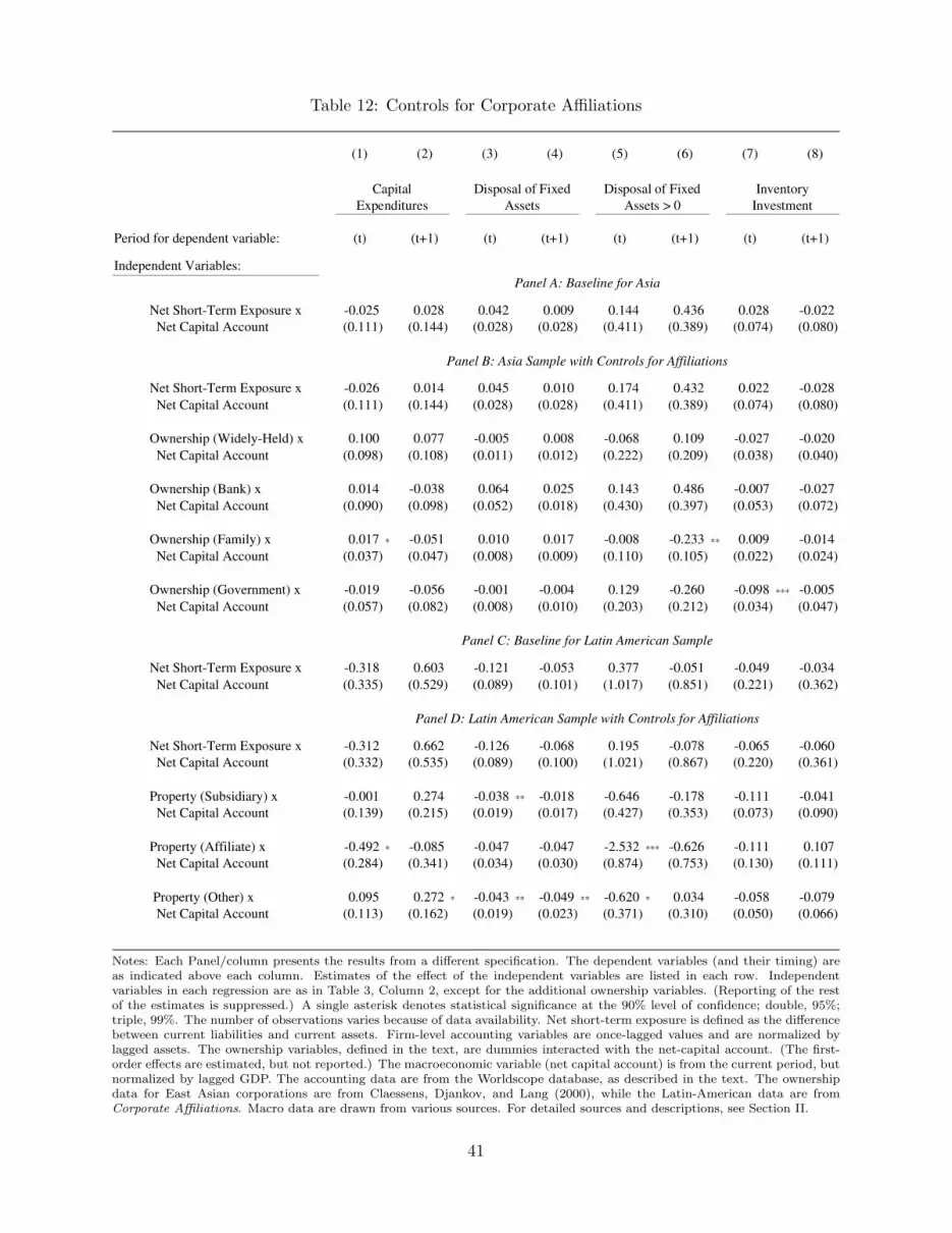
Table 12: Controls for Corporate Affiliations

(1) (2) (3) (4) (5) (6) (7) (8)

Period for dependent variable: (t) (t+1) (t) (t+1) (t) (t+1) (t) (t+1)

Independent Variables:Panel A: Baseline for Asia

Net Short-Term Exposure x -0.025 0.028 0.042 0.009 0.144 0.436 0.028 -0.022 Net Capital Account (0.111) (0.144) (0.028) (0.028) (0.411) (0.389) (0.074) (0.080)

Panel B: Asia Sample with Controls for Affiliations

Net Short-Term Exposure x -0.026 0.014 0.045 0.010 0.174 0.432 0.022 -0.028 Net Capital Account (0.111) (0.144) (0.028) (0.028) (0.411) (0.389) (0.074) (0.080)

Ownership (Widely-Held) x 0.100 0.077 -0.005 0.008 -0.068 0.109 -0.027 -0.020 Net Capital Account (0.098) (0.108) (0.011) (0.012) (0.222) (0.209) (0.038) (0.040)

Ownership (Bank) x 0.014 -0.038 0.064 0.025 0.143 0.486 -0.007 -0.027 Net Capital Account (0.090) (0.098) (0.052) (0.018) (0.430) (0.397) (0.053) (0.072)

Ownership (Family) x 0.017 * -0.051 0.010 0.017 -0.008 -0.233 ** 0.009 -0.014 Net Capital Account (0.037) (0.047) (0.008) (0.009) (0.110) (0.105) (0.022) (0.024)

Ownership (Government) x -0.019 -0.056 -0.001 -0.004 0.129 -0.260 -0.098 *** -0.005 Net Capital Account (0.057) (0.082) (0.008) (0.010) (0.203) (0.212) (0.034) (0.047)

Panel C: Baseline for Latin American Sample

Net Short-Term Exposure x -0.318 0.603 -0.121 -0.053 0.377 -0.051 -0.049 -0.034 Net Capital Account (0.335) (0.529) (0.089) (0.101) (1.017) (0.851) (0.221) (0.362)

Panel D: Latin American Sample with Controls for Affiliations

Net Short-Term Exposure x -0.312 0.662 -0.126 -0.068 0.195 -0.078 -0.065 -0.060 Net Capital Account (0.332) (0.535) (0.089) (0.100) (1.021) (0.867) (0.220) (0.361)

Property (Subsidiary) x -0.001 0.274 -0.038 ** -0.018 -0.646 -0.178 -0.111 -0.041 Net Capital Account (0.139) (0.215) (0.019) (0.017) (0.427) (0.353) (0.073) (0.090)

Property (Affiliate) x -0.492 * -0.085 -0.047 -0.047 -2.532 *** -0.626 -0.111 0.107 Net Capital Account (0.284) (0.341) (0.034) (0.030) (0.874) (0.753) (0.130) (0.111)

Property (Other) x 0.095 0.272 * -0.043 ** -0.049 ** -0.620 * 0.034 -0.058 -0.079 Net Capital Account (0.113) (0.162) (0.019) (0.023) (0.371) (0.310) (0.050) (0.066)

Capital Expenditures

Disposal of Fixed Assets

Disposal of Fixed Assets > 0

Inventory Investment

Notes: Each Panel/column presents the results from a different specification. The dependent variables (and their timing) areas indicated above each column. Estimates of the effect of the independent variables are listed in each row. Independentvariables in each regression are as in Table 3, Column 2, except for the additional ownership variables. (Reporting of the restof the estimates is suppressed.) A single asterisk denotes statistical significance at the 90% level of confidence; double, 95%;triple, 99%. The number of observations varies because of data availability. Net short-term exposure is defined as the differencebetween current liabilities and current assets. Firm-level accounting variables are once-lagged values and are normalized bylagged assets. The ownership variables, defined in the text, are dummies interacted with the net-capital account. (The first-order effects are estimated, but not reported.) The macroeconomic variable (net capital account) is from the current period, butnormalized by lagged GDP. The accounting data are from the Worldscope database, as described in the text. The ownershipdata for East Asian corporations are from Claessens, Djankov, and Lang (2000), while the Latin-American data are fromCorporate Affiliations. Macro data are drawn from various sources. For detailed sources and descriptions, see Section II.

41

Table 13: Financing and Short-Term Exposure

(1) (2) (3) (4) (5) (6) (7) (8) (9) (10) (11) (12)

Dependent Variables:

Independent Variables Total Debt Interest Payments Gross New Debt Net New Debtand Regression Statistics:

Panel A: Dependent Variables from the Current YearInteractions with Capital Flows:

Net Short-Term Exposure x -2.058 -0.131 -0.327 -0.133 -0.087 -0.152 0.371 0.268 0.580 -0.108 -0.112 -0.048 Net Capital Account (0.303) *** (0.387) (0.417) (0.033) *** (0.057) (0.055) *** (0.085) *** (0.192) (0.198) *** (0.100) (0.213) (0.234)

Leverage x -0.345 -0.671 0.072 -0.004 0.179 -0.162 -0.071 -0.146 Net Capital Account (0.293) (0.293) ** (0.050) (0.044) (0.182) (0.185) (0.181) (0.189)

Current Assets x 0.756 0.585 -0.085 -0.108 0.136 0.528 0.000 0.129 Net Capital Account -0.317 ** (0.336) * (0.048) * (0.045) ** (0.183) (0.181) *** (0.182) (0.187)

Controls:

Net Short-Term Exposure 0.593 0.032 0.018 0.050 0.001 -0.006 0.022 -0.049 -0.016 -0.022 -0.008 -0.004 (0.022) *** (0.029) (0.032) (0.002) *** (0.004) (0.004) * (0.006) *** (0.011) *** (0.012) (0.007) *** (0.013) (0.015)

Leverage 0.852 0.757 0.073 0.035 0.071 0.031 -0.022 -0.031 (0.024) *** (0.032) *** (0.003) *** (0.004) *** (0.010) *** (0.009) *** (0.011) * (0.013) **

Current Assets 0.033 0.023 -0.004 -0.006 -0.067 -0.032 -0.004 0.000 -0.023 (0.026) (0.003) (0.003) ** (0.011) *** (0.011) *** (0.011) (0.012)

Lagged Dependent Variable 0.086 0.558 0.202 0.105 (0.017) *** (0.022) *** (0.019) *** (0.013) ***

Regression Statistics:

N 19190 19185 15497 18643 18634 14883 14896 14887 11860 15402 15393 124090.34 0.58 0.59 0.38 0.48 0.62 0.11 0.12 0.17 0.12 0.12 0.14

Panel B: Dependent Variables from the Following YearInteractions with Capital Flows:

Net Short-Term Exposure x -1.880 -1.306 -2.058 -0.072 -0.017 -0.066 0.409 0.279 0.353 0.107 -0.142 -0.054 Net Capital Account (0.405) *** (0.535) ** (0.485) *** (0.038) * (0.059) (0.048) (0.106) *** (0.220) (0.196) * (0.105) (0.198) (0.188)

Leverage x 1.133 0.381 0.078 0.012 0.353 0.175 0.377 0.334 Net Capital Account (0.401) *** (0.353) (0.047) * (0.032) (0.204) * (0.169) (0.170) ** (0.134) **

Current Assets x -0.150 -1.251 -0.001 -0.026 0.244 0.290 -0.137 -0.111 Net Capital Account -0.480 (0.442) *** (0.050) (0.040) (0.199) (0.187) (0.176) (0.173)

Controls:

Net Short-Term Exposure 0.498 0.058 0.065 0.041 0.001 -0.001 0.012 -0.059 -0.022 -0.020 -0.003 0.010 (0.029) *** (0.038) (0.034) * (0.003) *** (0.004) (0.003) (0.009) (0.017) *** (0.014) (0.009) ** (0.015) (0.014)

Leverage 0.738 0.301 0.066 0.025 0.081 0.039 -0.011 -0.019 (0.029) *** (0.038) *** (0.004) *** (0.003) *** (0.014) *** (0.012) *** (0.011) (0.010) **

Current Assets 0.076 0.057 -0.001 0.001 -0.059 -0.031 0.021 0.019 -0.033 ** (0.030) * (0.004) (0.003) (0.014) *** (0.015) ** (0.012) * (0.013)

Lagged Dependent Variable 0.518 0.557 0.252 0.122 (0.028) *** (0.021) *** (0.033) *** (0.025) ***

Regression Statistics:

N 15564 15557 12452 15116 15110 11951 12403 12398 10079 12782 12777 105020.20 0.30 0.49 0.33 0.39 0.57 0.10 0.11 0.18 0.10 0.10 0.13

R2

R2

Notes: Each column reports the results of an OLS regression. The dependent variables are as indicated above each column.Estimates of the effect of the independent variables are listed in each row. Also included in each regression are indicator variablesfor each country-year cell. Huber-White standard errors are given in parentheses. A single asterisk denotes statistical significanceat the 90% level of confidence; double, 95%; triple, 99%. The number of observations varies because of data availability. Netshort-term exposure is defined as the difference between current liabilities and current assets. Firm-level independent variablesare once-lagged values. All accounting variables are scaled by the lag of total firm assets. The macroeconomic variable (netcapital account) s from the current period, but normalized by lagged GDP. The accounting data are from the Worldscopedatabase, as described in the text. Macro data are drawn from various sources. For detailed sources and descriptions, seeSection II.

42

Table 14: Income and Short-Term Exposure

Estimated Coefficient onNet Short-Term Exposure x

Net Capital AccountPeriod for Dependent Variable: (t) (t+1)

Dependent Variable:

Panel A: Full Sample

Income Variables

1. Operating Income 0.047 0.009 (0.097) (0.091)

2. Non Operating Income 0.602 0.112 (0.229) *** (0.155)

2.1 Income from investments -0.031 -0.008 (0.023) (0.023)

2.2 Accrued Interest Cost -0.152 -0.066 (0.055) *** (0.048)

2.3 Other Non Operating Income 0.338 0.126 (0.154) ** (0.089)

3. Net Income 0.859 0.092 (0.285) *** (0.188)

Cash Flow Variables

Cash flow from Operations 0.096 -0.032 (0.100) (0.096)

Earnings before interest, taxes and amortizations 0.786 -0.003 (0.268) *** (0.182)

Panel B: Subsample With Detailed Data

Other Non Operating Income 0.245 0.208 (0.107) ** (0.107) **

Gains from sale of assets 0.062 0.078 (0.033) * (0.032) **

Notes: Each cell reports the results of the estimated coefficient on (Net Short-Term Exposure × Net Capital Account) froman OLS regression. Independent variables in each regression are as in Table 3, Column 3, however reporting of the rest of theestimates is supressed. The dependent variable is listed in each row. Huber-White standard errors are reported in parenthesis.A single asterisk denotes statistical significance at the 90% level of confidence; double, 95%; triple, 99%. The sample variesacross dependent variables because of data availability. Net capital account is from the current period, but normalized by laggedGDP. The accounting data are from the Worldscope database. Definitions of the accounting variables are provided in the text.Macro data are drawn from various sources. For detailed sources and descriptions, see Section II.

43

Tab

le15

:In

vest

men

tE

last

icity

toC

apit

alFlo

ws:

Who

leE

cono

my

vs.

Sam

ple

ofC

orpo

rate

s

(1)

(2)

(3)

(4)

(5)

(6)

(7)

(8)

(9)

(10)

Inde

pend

ent V

aria

bles

P

anel

A: L

HS

is L

og (G

ross

Fix

ed C

apita

l For

mat

ion

in P

riva

te S

ecto

r)

Net

Cap

ital A

ccou

nt1.

850

***

1.79

2 **

2.55

0 **

*2.

504

***

2.33

3 **

*2.

375

***

(0.6

10)

(0.7

98)

(0.6

14)

(0.6

40)

(0.4

47)

(0.6

10)

NK

A x

Lat

in A

mer

ica

0.31

0 -0

.753

(1

.471

)(1

.321

)

Lag

ged

Dep

ende

nt V

aria

ble

0.70

4 **

*0.

521

***

(0.0

59)

(0.0

76)

Lag

ged

Net

Cap

ital A

ccou

nt3.

278

***

3.57

1 **

*3.

522

***

3.91

8 **

*

(0.5

77)

(0.7

72)

(0.5

60)

(0.5

65)

Tim

e T

rend

Yes

Yes

Tim

e T

rend

x C

ount

ry D

umm

yY

esY

esY

es

Pan

el B

: LH

S: L

og (C

apita

l Exp

endi

ture

s fr

om F

irm

Lev

el D

ata)

Net

Cap

ital A

ccou

nt2.

277

***

1.71

1 **

*2.

992

***

3.16

1 **

*2.

323

***

3.28

7 **

*

(0.3

57)

(0.4

52)

(0.3

21)

(0.3

73)

(0.3

23)

(0.4

03)

NK

A x

Lat

in A

mer

ica

1.84

7 **

1.42

5 *

(0.8

34)

(0.7

39)

Lag

ged

Dep

ende

nt V

aria

ble

0.28

5 **

*0.

188

***

(0.0

43)

(0.0

51)

Lag

ged

Net

Cap

ital A

ccou

nt2.

840

***

2.38

2 **

*3.

067

***

3.28

2 **

*

(0.3

35)

(0.4

31)

(0.3

02)

(0.3

50)

Tim

e T

rend

Yes

Yes

Tim

e T

rend

x C

ount

ry D

umm

yY

esY

esY

es

Note

s:E

ach

Panel

/C

olu

mn

conta

ins

the

resu

lts

from

ase

para

tere

gre

ssio

noflo

gari

thm

icin

ves

tmen

tgro

wth

on

the

net

capitalacc

ount.

InPanel

A,th

edep

enden

tvari

able

isco

nst

ruct

edfr

om

data

on

the

gro

ssfixed

-capit

alfo

rmati

on

ofth

epri

vate

sect

or.

The

capitalex

pen

dit

ure

sfr

om

Worl

dsc

ope

sam

ple

des

crib

edin

Sec

tion

IIare

use

dto

form

the

inves

tmen

tm

easu

re.

Countr

yfixed

effec

tsare

incl

uded

inea

chsp

ecifi

cation,but

not

report

ed.

44

Appendix: Data Sources and Definitions

This appendix describes our main variables and sources.

VII.A Sources and definitions for the firm-level data

Our main source of firm level data is the Worldscope Database. There are two main types offirm level data: accounting variables, and non-accounting variables. The first come directly fromfirm Balance Sheets, Income Statements and Cash-Flow Statements. The second correspond toadditional information regarding firm ownership, and production structure. Examples of the latterare whether a firm has a listed stock, where this stock is traded, and the sector where the firmis operating. The only firm level variables not from Worldscope are the ADR dummy, whichidentifies whether the firm trades shares in the form of American Depositary Receipts (ADRs), andthe variables identifying firms as part of a conglomerate.

The codes correspond to the codes from Worldscope database. Unless specified otherwise allaccounting variables are scaled by lagged total assets (WS 02999).

Accounting Variables

Investment

• Capital Expenditures: This variable corresponds to the funds spent by the firm on fixed assets(WS 04601).

• Disposal of Fixed Assets: Sales of fixed assets (WS 04351).

• Change in Inventories: This variable corresponds to the change in inventories (WS 02101)between the current and previous year.

Main control variables

• Exposure: This variable is measured as the difference between lagged current liabilities (WS03101) and lagged current assets.

• Leverage: Lagged total liabilities (WS 03351).

• Current Assets: Lagged current assets (WS 02201).

Financing variables

• Interest Accruals: Interest expenses on debt (WS 01251).

• Gross New Debt: This variable corresponds to new debt issuance. It includes both short-termand long-term debt. It is constructed as long-term borrowings (WS 04401) plus net shortterm borrowings (WS 04821).

• Net New Debt: This variable corresponds to debt issuance, net of debt repayments. Itincludes both short-term and long-term debt. It is constructed as long-term borrowings (WS04401) minus the reduction in long-term debt (WS 04701) plus net short term borrowings(WS 04821).

45

Income variables

• Operating Income: Income from firm’s main line of operations (WS 01250).

• Net Income: This variable correspond to net income after preferred dividends (WS 01706).

• Non Operating Income: Is the difference between Operating Income (WS 01250) and NetIncome (WS 01706).

• Income from Investments: This variable is a sub-category of Non Operating Income. It is thesum of: Non Operating Interest Income (WS 01266), Pretax Equity Earnings (WS 01267)and Equity in Earnings (WS 1503).

• Other Non Operating Income: This variable is a sub-category of Non Operating Income. Itis the sum of Other Income (WS 01262) and After Tax Other Income (WS 01540).

• Gains from Sales of Assets: This variable is a supplementary variable to the income statement.It is included in Other Non Operating Income, and corresponds to accounting gains/lossesfrom the sale of assets (WS 01306).

• Cash Flow from operations (WS 04201).

• EBITDA: This variable correspond to the earnings before interest expense, income taxes anddepreciation (WS 18198).

Non-Accounting Variables

• ADR: This is a indicator variable that measures wether the firm’s stock is listed in a US stockexchange in the form of American Depository Receipts. The variable was constructed usinginformation from the Bank of New York.

• Cross-listing: This is a indicator variable that takes on value 1 wether the firm’s stock istraded in more than one stock exchange. It was constructed using (WS 20009)

• Listed on a stock exchange: This is a indicator variable that take the value 1 wether the firmhas a stock listed in a stock exchange (WS 20009).

• SIC code: Standard Industrial Classification code (version 1987) (WS 07021)

• Export dummy: dummy if firm exported (WS 07161) in previous period.

Property Data

• For firms from East Asia, the source of data on firm ownership is Claessens, Djankov andLang (2000). The first category is for widely held firms. The additional three categories are:firms affiliated with banks, firms affiliated with families and firms affiliated with governments.The omitted category is for those firms not classified in that study. Data refer to ownershipstatus in 1996.

• For Latin America, we build ownership variables using the June 2003 version of the CorporateAffiliations Plus database (Lexis-Nexis, 2003). This database classifies firms into subsidiaries,affiliates and widely held corporations. The omitted category is for firms not appearing inthe Corporate Affiliations database.

46

VII.B Sources and Definitions for the Macroeconomic Data

All the aggregate variables are based on data from the International Financial Statistics, (IMF,2004a) with the exception of the Sudden Stop Dummy which comes from Calvo, Izquierdo, Mejia.(2004).

VII.B.1 Capital Flows

• Net Capital Inflows: Net financial account (IFS 78bjd) expressed in previous period localcurrency, scaled by lagged nominal GDP (IFS 99b). For previous period local currencyUS Dollar Balance of Payments variables are multiplied by the once lagged period averageexchange rate (local currency × US Dollar).

• Capital Inflows net of FDI: This variable corresponds to Net Financial Account (IFS 78bjd)net of Direct Investment Abroad (IFS 78bdd) and Direct Investment in Reporting Economy(IFS 78bed), expressed in previous period local currency, scaled by lagged nominal GDP.

• Change in Credit to the Private Sector: This variable corresponds to the cpi-adjusted changein bank credit to private sector (IFS 22d) scaled by nominal GDP.

VII.B.2 Alternative Measures of Capital Flows

• Low Capital Inflow (low): This is a indicator variable that takes a value of 1 when the NetFinancial Account (IFS 78bjd) is below a threshold z, where z is defined as the median valueof the Net Financial Account in the period between 1985 and 2002 per country.

• Crisis Inflow (crisis) : This is a indicator variable that takes a value of 1 when the NetFinancial Account (IFS 78bjd) is below a threshold x, where x is the mean value minusone standard deviation of the Net Financial Account over the period 1985 to 2002 for eachcountry.

• Stop in Capital Inflows (stop): This is a indicator variable that takes on a value of 1 fornegative changes in Net Capital Inflows.

• Sudden Stop: From Calvo et al. (2004). The authors define a Sudden Stop as a phase thatmeets the following conditions:

1. It contains at least one observation where the year-on-year fall in capital flows lies atleast two standard deviations below its sample mean.

2. The Sudden Stop phase ends once the annual change in capital flows exceeds one standarddeviation below its sample mean.

3. Moreover, for the sake of symmetry, the start of a Sudden Stop phase is determined bythe first time the annual change in capital flows falls one standard deviation below themean.

4. The episode must lead to a costly disruption in economic activity, defined as a contractionin output.

For the episode section, we work with the first year in the Calvo et al’s sudden-stop event.

47

VII.B.3 Aggregate Investment

• We built aggregate investment data in our sample using the Capital Expenditures variabledescribed above. To control for the effects of changes in sample size we aggregate annualpercentage changes in firm capital expenditure Iict, to construct the aggregate percentagechange in total sample investment Ict, such that

Ict =n∑

i=1

αict−1Iict

where αict−1 is the share of capital expenditures of firm i in total expenditures of country cin period t− 1.

• Economy-wide investment data is Private Gross Fixed Capital Formation from the WorldEconomic Outlook of the IMF (IMF 2004b). For Korea and Indonesia, we complement theIMF data with a series on private investment from Everhart and Sumlinski (2001).

• Both investment series are deflated by period average CPI from the International FinancialStatistics, (IMF, 2004a).

48

Appendix Table 1: Robustness to Sample Changes

Dependent Variables:

Capital Expenditures Inventory Investment

Period for dependent variable: (t) (t+1) (t) (t+1) (t) (t+1) (t) (t+1)

Independent Variables: Baseline Sample: Outliers z-score>6, synthetic firms, imputed values for bankrupt firms

Net Short-Term Exposure x 0.015 0.075 0.052 0.004 -0.062 0.282 0.036 -0.039 Net Capital Account (0.093) (0.134) (0.026) ** (0.026) (0.346) (0.326) (0.064) (0.072)

Number of Observations 13943 11362 11613 9864 20023 20023 14238 11598

Sample 2: Outliers z-score>6, synthetic firms, no imputed values for bankrupt firms

Net Short-Term Exposure x 0.015 0.075 0.050 0.004 -0.051 0.293 0.036 -0.039 Net Capital Account (0.093) (0.134) (0.026) * (0.026) (0.346) (0.326) (0.064) (0.072)

Number of Observations 13938 11362 11609 9864 20016 20016 14233 11598

Sample 3: Outliers z-score>6, no synthetic firms, imputed values for bankrupt firms

Net Short-Term Exposure x 0.018 0.078 0.056 0.008 0.057 0.432 0.047 -0.042 Net Capital Account (0.093) (0.134) (0.026) ** (0.026) (0.345) (0.326) (0.063) (0.072)

Number of Observations 14322 11666 11821 10041 20523 20523 14645 11922

Sample 4: Outliers z-score>6, no synthetic firms, no imputed values for bankrupt firms

Net Short-Term Exposure x 0.018 0.078 0.054 0.008 0.068 0.442 0.047 -0.042 Net Capital Account (0.093) (0.134) (0.026) ** (0.026) (0.345) (0.325) (0.063) (0.072)

Number of Observations 14317 11666 11817 10041 20516 20516 14640 11922

Sample 5: Outliers top and bottom 1%, synthetic firms, imputed values for bankrupt firms

Net Short-Term Exposure x -0.031 -0.032 0.055 0.004 -0.094 0.301 0.029 0.045 Net Capital Account (0.072) (0.084) (0.022) ** (0.024) (0.388) (0.360) (0.053) (0.057)

Number of Observations 13423 10964 11294 9599 19511 19511 13642 11072

Sample 6: Outliers top and bottom 1%, synthetic firms, no imputed values for bankrupt firms

Net Short-Term Exposure x -0.030 -0.032 0.054 0.004 -0.082 0.313 0.027 0.045 Net Capital Account (0.072) (0.084) (0.022) ** (0.024) (0.388) (0.360) (0.053) (0.057)

Number of Observations 13418 10964 11291 9599 19504 19504 13639 11072

Sample 7: Outliers top and bottom 1%, no synthetic firms, imputed values for bankrupt firms

Net Short-Term Exposure x -0.025 -0.034 0.056 0.008 0.008 0.464 0.038 0.037 Net Capital Account (0.072) (0.084) (0.022) ** (0.024) (0.386) (0.359) (0.053) (0.057)

Number of Observations 13787 11261 11490 9764 19994 19994 14031 11386

Sample 8: Outliers top and bottom 1%, no synthetic firms, no imputed values for bankrupt firms

Net Short-Term Exposure x -0.024 -0.034 0.056 0.008 0.021 0.476 0.036 0.037 Net Capital Account (0.072) (0.084) (0.022) ** (0.024) (0.386) (0.359) (0.053) (0.057)

Number of Observations 13782 11261 11487 9764 19987 19987 14028 11386

Disposal of Fixed Assets

Disposal of Fixed Assets>0

Notes: Each panel presents the results using a different sample. Each cell reports the results of an OLS regression. Thedependent variables are as indicated above each column. Estimates of the effect of the indicated short-term exposure variabletimes the capital inflow variable are listed in each cell. Independent variables in each regression are as in Table 3, Column 2,however reporting of the rest of the estimates is supressed. A single asterisk denotes statistical significance at the 90% levelof confidence; double, 95%; triple, 99%. Net capital account is from the current period, but normalized by lagged GDP. Theaccounting data are from the Worldscope database, as described in the text. Macro data are drawn from various sources. Fordetailed sources and descriptions, see Section II.

49