1

DESCRIPTIVE STATISTICS By Ive Barreiros

Statistics has two major chapters

• Descriptive Statistics • Inferential statistics

Descriptive Statistics. It provides mathematical and graphic procedures to summarize the information of the data in a clear and understandable way. The tools in descriptive statistics are graphical presentations and mathematical formulas.

Inferential Statistics. It provides procedures to draw inferences (to say something) about a population from results

obtained from a subset of the units in the population (sample). In order to give some measure of the reliability of those

inferences, statistics uses probability concepts.

1 – Population and Sample

Any set of individuals (or objects) having some common observable characteristic constitutes a population, or

universe of study. Any subset of a population is a sample from that population. The term population may refer to the individuals measured or to the measurements themselves. There will be a

“distribution of measurements of the sample”, which we actually observe and study, and a “distribution of measurements in the population”, which may exist (but usually do not), in an observed and recorded form. One of the most important

problems in Statistics is to decide what information about a distribution of the population can be inferred from the study

of a sample. A third type of distribution consists of the distribution of a “measure” computed on each of the possible samples

of a fixed size which could be taken from a population1. For example, if we take all the possible samples of 100 students from the student body currently enrolled in our school and compute the mean age of each sample, we will have a good

number of means. These means form a distribution, which is called the sampling distribution of the mean of samples of

size 100.

Here we present some examples of population and samples:

1. In a survey of mathematical ability of seventh graders in rural areas, a mathematical ability test was given to 300 children enrolled in 7th grade in rural areas. The universe would be all seventh graders in

rural areas; the sample would be the 300 children taking the test.

2. An investigation is being undertaken to test the effects of a particular type of drug on certain specific infectious process. A group of rats is infected and treated with the drug. Then the proportion of rats

that recovered in a specific time is observed. The universe or population consists of all the rats which will be, or could be, infected and then given the drug. The sample consists of the group of rats actually

used, and the measurable characteristic is either recovery or failure to recover within the specified time

1 Some authors refer to the “population “ by the term “universe” or “universe under study”

2

interval. The universe or population here cannot be observed since we could not perform the

experiment on every rat. 3. A survey is made to determine the opinion of people in a certain county on a proposed county law. A

sample of 500 people residing in the county is questioned, and the number of favorable opinions is recorded. Here the population or universe consists of all people living in the county (with probably a

lower limit of age). The sample consists of the 500 that were inquired; the characteristic of interest is

whether the person has a favorable or unfavorable opinion regarding the proposed law.

2 - Populations A population or universe can be finite (grade school students in a city, animals in a geographical area, light bulbs

manufactured during a day, etc.), or it can be infinite (all points on the plane, all weights between 7 pounds and 8

pounds, the time requires for kindergarten children to put together a puzzle). In some cases the universe is so large that should be consider infinite (a bag of grain, pine trees on a mountain, etc.).

The population size will be denoted by N and the sample size will denoted by n.

Measures computed by using all the measurements in the population will be called parameters. They will be indicated

by Greek letters. For example the mean or simple average of the population will be denoted by .

Measured computed by using all the measurements in a sample will be called “statistics”. For example the mean or simple

average of the sample is called sample mean and denoted by x .

Example of a finite population

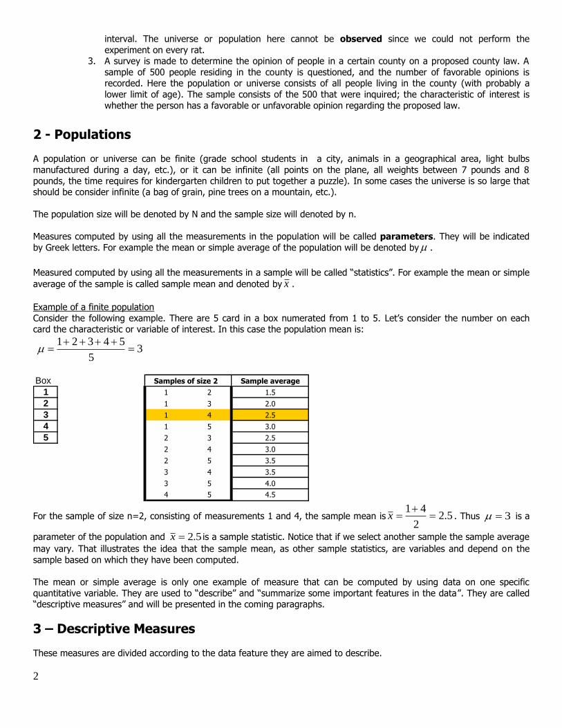
Consider the following example. There are 5 card in a box numerated from 1 to 5. Let’s consider the number on each card the characteristic or variable of interest. In this case the population mean is:

35

54321

Box Samples of size 2 Sample average

1 1 2 1.5

2 1 3 2.0

3 1 4 2.5

4 1 5 3.0

5 2 3 2.5

2 4 3.0

2 5 3.5

3 4 3.5

3 5 4.0

4 5 4.5

For the sample of size n=2, consisting of measurements 1 and 4, the sample mean is 5.22

41

x . Thus 3 is a

parameter of the population and 5.2x is a sample statistic. Notice that if we select another sample the sample average

may vary. That illustrates the idea that the sample mean, as other sample statistics, are variables and depend on the

sample based on which they have been computed.

The mean or simple average is only one example of measure that can be computed by using data on one specific

quantitative variable. They are used to “describe” and “summarize some important features in the data”. They are called “descriptive measures” and will be presented in the coming paragraphs.

3 – Descriptive Measures

These measures are divided according to the data feature they are aimed to describe.

3

Central Tendency measures. They are computed in order to give a “center” around which the measurements in

the data are distributed. Variation or Variability measures. They describe “data spread” or how far away the measurements are from the

center. Relative Standing measures. They describe the relative position of a specific measurement in the data

3.1- Measures of Central Tendency

Mean: Sum of all measurements in the data divided by the number of measurements.

Consider the following data and assume that it corresponds to a sample of size n=8 : {5,4,7,3,1,3,4,5} . The sample

mean is 48

54313745

x

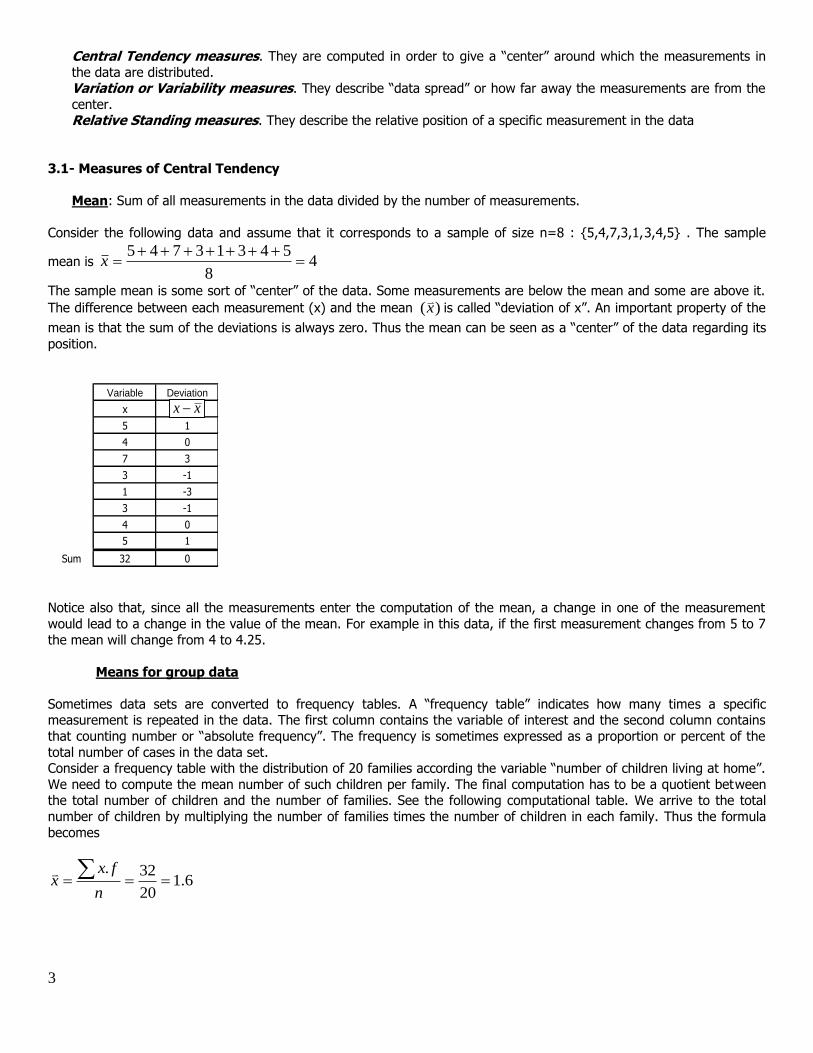
The sample mean is some sort of “center” of the data. Some measurements are below the mean and some are above it.

The difference between each measurement (x) and the mean )(x

is called “deviation of x”. An important property of the

mean is that the sum of the deviations is always zero. Thus the mean can be seen as a “center” of the data regarding its

position.

Variable Deviation

x

5 1

4 0

7 3

3 -1

1 -3

3 -1

4 0

5 1

Sum 32 0

xx

Notice also that, since all the measurements enter the computation of the mean, a change in one of the measurement

would lead to a change in the value of the mean. For example in this data, if the first measurement changes from 5 to 7

the mean will change from 4 to 4.25.

Means for group data

Sometimes data sets are converted to frequency tables. A “frequency table” indicates how many times a specific measurement is repeated in the data. The first column contains the variable of interest and the second column contains

that counting number or “absolute frequency”. The frequency is sometimes expressed as a proportion or percent of the

total number of cases in the data set. Consider a frequency table with the distribution of 20 families according the variable “number of children living at home”.

We need to compute the mean number of such children per family. The final computation has to be a quotient between the total number of children and the number of families. See the following computational table. We arrive to the total

number of children by multiplying the number of families times the number of children in each family. Thus the formula

becomes

6.1

20

32.

n

fxx

4

X f x.f

0 4 0

1 5 5

2 7 14

3 3 9

4 1 4

Sum 20 32

If the frequency table has the cases grouped in classes (“class table”) the value of x should represent the whole class. It is the mid value of each class limits. It is called “class mark” and denoted by

x . An example follows

Class (x) Frequency Class marks (x*) f x*.f

5 to 9 18 7 18 126

10 to 14 48 12 48 576

15 to 19 57 17 57 969

20 to 24 25 22 25 550

25 to 29 12 27 12 324

Total 160 Total 160 2545

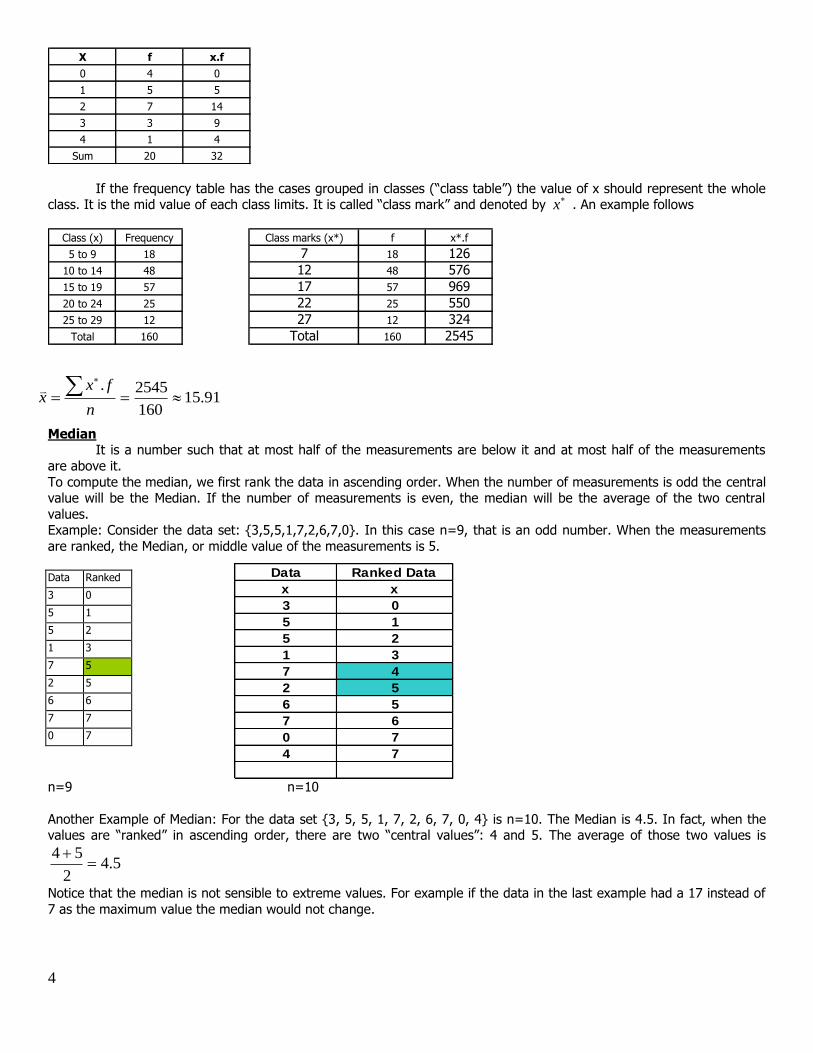
Median It is a number such that at most half of the measurements are below it and at most half of the measurements

are above it.

To compute the median, we first rank the data in ascending order. When the number of measurements is odd the central value will be the Median. If the number of measurements is even, the median will be the average of the two central

values. Example: Consider the data set: {3,5,5,1,7,2,6,7,0}. In this case n=9, that is an odd number. When the measurements

are ranked, the Median, or middle value of the measurements is 5. Data Ranked

3 0

5 1

5 2

1 3

7 5

2 5

6 6

7 7

0 7

n=9 n=10

Another Example of Median: For the data set {3, 5, 5, 1, 7, 2, 6, 7, 0, 4} is n=10. The Median is 4.5. In fact, when the values are “ranked” in ascending order, there are two “central values”: 4 and 5. The average of those two values is

5.42

54

Notice that the median is not sensible to extreme values. For example if the data in the last example had a 17 instead of

7 as the maximum value the median would not change.

91.15160

2545.

n

fxx

Data Ranked Data

x x

3 0

5 1

5 2

1 3

7 4

2 5

6 5

7 6

0 7

4 7

5

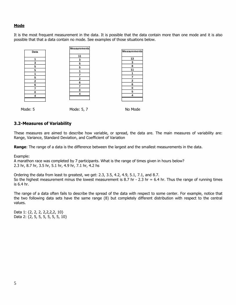
Mode

It is the most frequent measurement in the data. It is possible that the data contain more than one mode and it is also

possible that that a data contain no mode. See examples of those situations below.

Mode: 5 Mode: 5, 7 No Mode

3.2-Measures of Variability

These measures are aimed to describe how variable, or spread, the data are. The main measures of variability are: Range, Variance, Standard Deviation, and Coefficient of Variation

Range: The range of a data is the difference between the largest and the smallest measurements in the data.

Example: A marathon race was completed by 7 participants. What is the range of times given in hours below?

2.3 hr, 8.7 hr, 3.5 hr, 5.1 hr, 4.9 hr, 7.1 hr, 4.2 hs

Ordering the data from least to greatest, we get: 2.3, 3.5, 4.2, 4.9, 5.1, 7.1, and 8.7.

So the highest measurement minus the lowest measurement is 8.7 hr - 2.3 hr = 6.4 hr. Thus the range of running times is 6.4 hr.

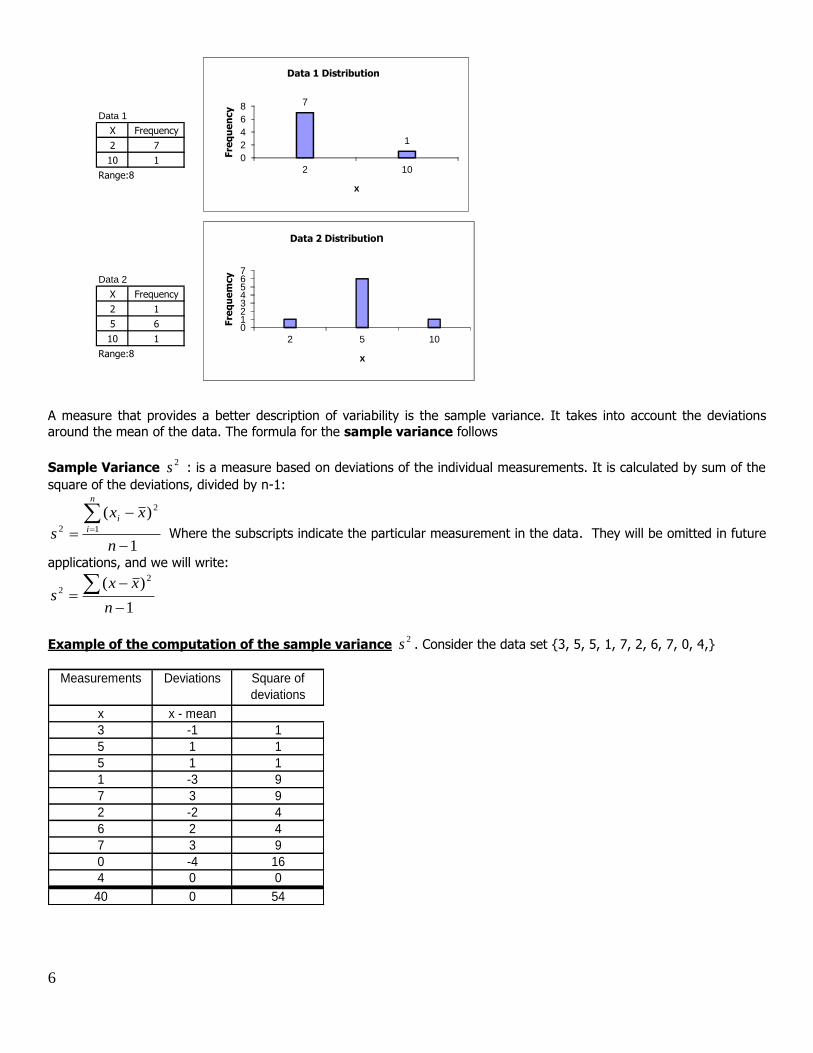
The range of a data often fails to describe the spread of the data with respect to some center. For example, notice that

the two following data sets have the same range (8) but completely different distribution with respect to the central values.

Data 1: {2, 2, 2, 2,2,2,2, 10} Data 2: {2, 5, 5, 5, 5, 5, 5, 10}

Data

1

3

5

5

1

5

2

6

7

0

4

Measurements

11

3

5

5

1

7

2

6

7

0

4

Measurements

13

3

8

11

1

7

2

6

0

5

4

6

Data 1

X Frequency

2 7

10 1

Range:8

Data 2

X Frequency

2 1

5 6

10 1

Range:8

7

1

0

2

4

6

8

2 10

Fre

qu

en

cy

x

Data 1 Distribution

01234567

2 5 10

Fre

qu

em

cy

x

Data 2 Distribution

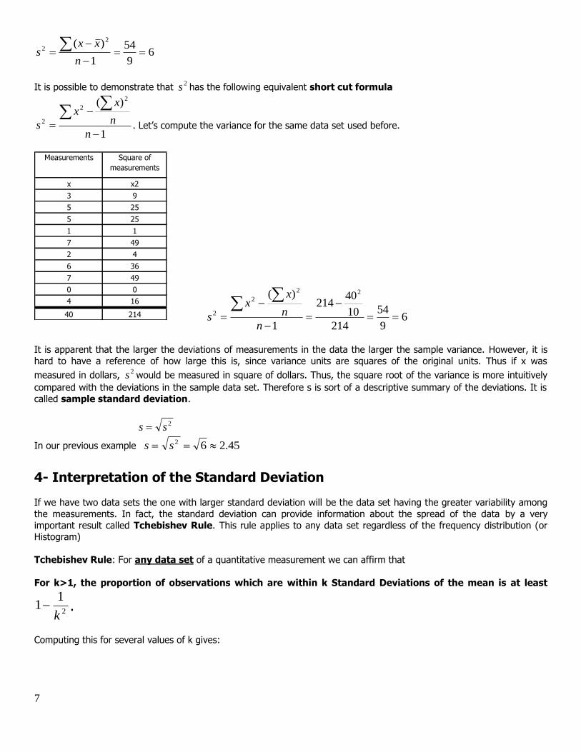
A measure that provides a better description of variability is the sample variance. It takes into account the deviations

around the mean of the data. The formula for the sample variance follows

Sample Variance 2s : is a measure based on deviations of the individual measurements. It is calculated by sum of the

square of the deviations, divided by n-1:

1

)( 2

12

n

xx

s

n

i

i

Where the subscripts indicate the particular measurement in the data. They will be omitted in future

applications, and we will write:

1

)( 2

2

n

xxs

Example of the computation of the sample variance 2s . Consider the data set {3, 5, 5, 1, 7, 2, 6, 7, 0, 4,}

Measurements Deviations Square of

deviations

x x - mean

3 -1 1

5 1 1

5 1 1

1 -3 9

7 3 9

2 -2 4

6 2 4

7 3 9

0 -4 16

4 0 0

40 0 54

7

69

54

1

)( 2

2

n

xxs

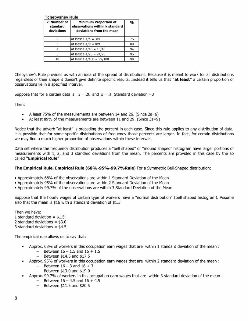
It is possible to demonstrate that 2s has the following equivalent short cut formula

1

)( 2

2

2

n

n

xx

s . Let’s compute the variance for the same data set used before.

Measurements Square of

measurements

x x2

3 9

5 25

5 25

1 1

7 49

2 4

6 36

7 49

0 0

4 16

40 214 69

54

214

10

40214

1

)( 22

2

2

n

n

xx

s

It is apparent that the larger the deviations of measurements in the data the larger the sample variance. However, it is

hard to have a reference of how large this is, since variance units are squares of the original units. Thus if x was

measured in dollars, 2s would be measured in square of dollars. Thus, the square root of the variance is more intuitively

compared with the deviations in the sample data set. Therefore s is sort of a descriptive summary of the deviations. It is

called sample standard deviation.

2ss

In our previous example 45.262 ss

4- Interpretation of the Standard Deviation If we have two data sets the one with larger standard deviation will be the data set having the greater variability among

the measurements. In fact, the standard deviation can provide information about the spread of the data by a very

important result called Tchebishev Rule. This rule applies to any data set regardless of the frequency distribution (or Histogram) Tchebishev Rule: For any data set of a quantitative measurement we can affirm that

For k>1, the proportion of observations which are within k Standard Deviations of the mean is at least

2

11

k .

Computing this for several values of k gives:

8

Tchebyshev Rule k: Number of

standard

deviations

Minimum Proportion of

observations within k standard

deviations from the mean

%

2 At least 1-1/4 = 3/4 75

3 At least 1-1/9 = 8/9 89

4 At least 1-1/16 = 15/16 94

5 At least 1-1/25 = 24/25 95

10 At least 1-1/100 = 99/100 99 Chebyshev’s Rule provides us with an idea of the spread of distributions. Because it is meant to work for all distributions regardless of their shape it doesn’t give definite specific results. Instead it tells us that “at least” a certain proportion of

observations lie in a specified interval.

Suppose that for a certain data is: 20x and 3s Standard deviation =3

Then:

• A least 75% of the measurements are between 14 and 26. (Since 2s=6)

• At least 89% of the measurements are between 11 and 29. (Since 3s=9)

Notice that the adverb “at least” is preceding the percent in each case. Since this rule applies to any distribution of data,

it is possible that for some specific distributions of frequency those percents are larger. In fact, for certain distributions we may find a much higher proportion of observations within these intervals.

Data set where the frequency distribution produces a “bell shaped” or “mound shaped” histogram have larger portions of

measurements with 1, 2, and 3 standard deviations from the mean. The percents are provided in this case by the so called “Empirical Rule”

The Empirical Rule. Empirical Rule (68%-95%-99.7%Rule) For a Symmetric Bell-Shaped distribution;

• Approximately 68% of the observations are within 1 Standard Deviation of the Mean • Approximately 95% of the observations are within 2 Standard Deviation of the Mean

• Approximately 99.7% of the observations are within 3 Standard Deviation of the Mean

Suppose that the hourly wages of certain type of workers have a “normal distribution” (bell shaped histogram). Assume

also that the mean is $16 with a standard deviation of $1.5

Then we have: 1 standard deviation = $1.5

2 standard deviations = $3.0

3 standard deviations = $4.5

The empirical rule allows us to say that:

• Approx. 68% of workers in this occupation earn wages that are within 1 standard deviation of the mean :

– Between 16 – 1.5 and 16 + 1.5 – Between $14.5 and $17.5

• Approx. 95% of workers in this occupation earn wages that are within 2 standard deviation of the mean : – Between 16 – 3 and 16 + 3

– Between $13.0 and $19.0

• Approx. 99.7% of workers in this occupation earn wages that are within 3 standard deviation of the mean : – Between 16 – 4.5 and 16 + 4.5

– Between $11.5 and $20.5

9

The sample Coefficient of Variation (CV) It is a normalized measure of variation of a data distribution. It is defined as the ratio of the standard deviation s to the mean x . It is often reported as a percentage (%) by multiplying the indicated relation by 100.

100x

sCV

Note; this is only defined for non-zero mean, and is most useful for variables that are always positive.

5 - Relative Standing Measures

We have seen that the median of a data set divides the ranked data into two equal parts: the bottom 50% and the top 50%. The percentiles divide the data set, once ranked into hundreds, or 100 equal parts.

Roughly speaking, the percentile P1 is a number that divides the ranked data into the bottom 1% and to top 99%. The second percentile, P2, divides the data into the bottom 2% and the top 98%.

Notice that the median is the 50th percentile (P50).

Deciles D1, D2, D3, and D9 are 9 numbers that divide the ranked data into 10 groups. The decile D1 divides the data into

the bottom 10% and the top 90%. D2 divides the ranked data into the bottom 20% and the top 80%. And so forth.

The most commonly used percentiles are the quartiles. They divide the data in four groups. A data have three quartiles,

denoted by Q1, Q2, and Q3. The first quartile Q1 is a number that divides the button 25% from the top 75% of measurements in the data set. The second quartile is the median. That is the number that divides the bottom 50% form

the top 50%. The third quartile is the umber that divides the bottom 75% from the top 25%. Note that Q1 and Q3 are

P25 and P75 respectively.

Here we have presented the intuitive definitions of percentiles and quartiles. More precise definitions are necessary if we need to actually compute the measure

If a data contain n measurements of a variable x, the computation of quartiles requires the following steps:

Rank the data Q1 is at the position (n+1)/4

Q2 is at the position (n+1)/2 (Q2 is the median) Q3 is at the position (n+1)(3/4).

If the position is not a whole number it will require linear extrapolation.

10

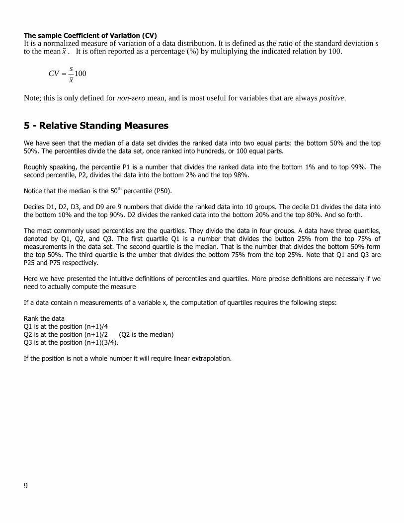
Example of Computation of Quartiles

Data (x) Sorted (x) Rank (n+1)x0.25=21x0.25= 5.25 (rank of Q1)

7 7 1 Incremente from 5th to 6th = 19 -17 = 2

34 7 2 Add to 5th measurement (2x0.25 ) = 0.5

92 13 3 Extrapolation Q1=17+0.5=17.5

37 14 4 Q1 =17.5

14 17 5

19 19 6

27 19 7

63 27 8 (n+1)x0.5=21x0.25= 21x 0.50=10.5 (rank of Q2)

98 27 9 Incremente from 10th to 11th = 34 -32 = 2

35 32 10 Add to 10th measurement (2x0.5 ) = 1

13 34 11 Extrapolation Q2=32+ 1= 33

7 35 12 Q2 (or median) = 33

32 37 13

51 51 14

17 54 15

19 58 16 (n+1)x0.75 = 21x0.75= 15.75 (rank of Q3)

63 63 17 Incremente from 5th to 6th = 58-54 =4

54 63 18 Add to 5th measurement (4x0.25 ) = 1

27 92 19 Extrapolation Q1=54+1=55

58 98 20 Q3 =55

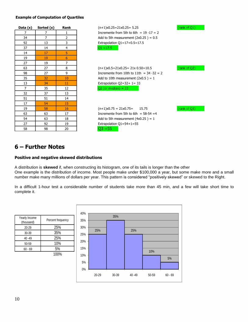
6 – Further Notes Positive and negative skewed distributions

A distribution is skewed if, when constructing its histogram, one of its tails is longer than the other

One example is the distribution of income. Most people make under $100,000 a year, but some make more and a small

number make many millions of dollars per year. This pattern is considered “positively skewed” or skewed to the Right.

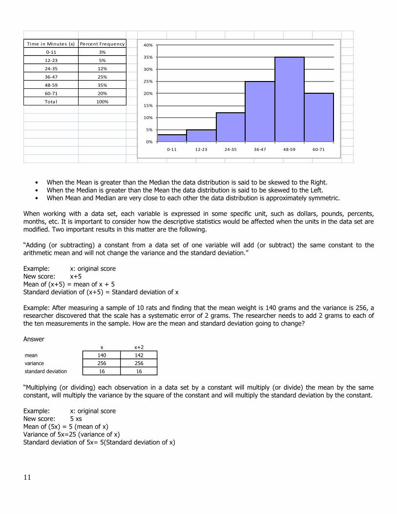
In a difficult 1-hour test a considerable number of students take more than 45 min, and a few will take short time to

complete it.

Yearly Income

(thousand)Percent frequency

20-29 25%

30-39 35%

40 -49 25%

50-59 10%

60 - 69 5%

100%

25%

35%

25%

10%

5%

0%

5%

10%

15%

20%

25%

30%

35%

40%

20-29 30-39 40 -49 50-59 60 - 69

11

Time in Minutes (x) Percent Frequency

0-11 3%

12-23 5%

24-35 12%

36-47 25%

48-59 35%

60-71 20%

Total 100%

0%

5%

10%

15%

20%

25%

30%

35%

40%

0-11 12-23 24-35 36-47 48-59 60-71

• When the Mean is greater than the Median the data distribution is said to be skewed to the Right.

• When the Median is greater than the Mean the data distribution is said to be skewed to the Left. • When Mean and Median are very close to each other the data distribution is approximately symmetric.

When working with a data set, each variable is expressed in some specific unit, such as dollars, pounds, percents,

months, etc. It is important to consider how the descriptive statistics would be affected when the units in the data set are

modified. Two important results in this matter are the following.

“Adding (or subtracting) a constant from a data set of one variable will add (or subtract) the same constant to the arithmetic mean and will not change the variance and the standard deviation.”

Example: x: original score New score: x+5

Mean of (x+5) = mean of x + 5 Standard deviation of (x+5) = Standard deviation of x

Example: After measuring a sample of 10 rats and finding that the mean weight is 140 grams and the variance is 256, a researcher discovered that the scale has a systematic error of 2 grams. The researcher needs to add 2 grams to each of

the ten measurements in the sample. How are the mean and standard deviation going to change?

Answer x x+2

mean 140 142

variance 256 256

standard deviation 16 16

“Multiplying (or dividing) each observation in a data set by a constant will multiply (or divide) the mean by the same constant, will multiply the variance by the square of the constant and will multiply the standard deviation by the constant.

Example: x: original score New score: 5 xs

Mean of (5x) = 5 (mean of x) Variance of 5x=25 (variance of x)

Standard deviation of 5x= 5(Standard deviation of x)

12

Example: An economist has a data set containing the population of Latin American and Caribbean countries measured in

number of people. He decides to present the descriptive statistics in thousands of people. Thus each number in the data will be divided by 1,000. How are the mean, variance and standard deviation changed?

Answer

Population in people Population in thousand people

Mean 12,372,342 12,372

Standard Deviation 31,081,527 31,082

Sample Variance 966,061,329,368,300 966,061,329

7 - Z Scores

Scores in data sets are, as pointed out before, arbitrary constructed type of observations (age of people in years, last year family income in thousand dollars, weight of a new born baby in pounds, etc. In dealing with different series of

observations, it is sometimes desirable to have scores that are easily compared. We reduce the x-score in the data set to

the so called “z- score”, by the formula:

s

xxz

Notice that a measurement x that is larger than the mean will have a positive z-score. Similarly, a measurement that is less that the mean will have a negative z- score. The z- score is zero for x=mean.

It is important to notice that the z-score consists of expressing the deviation xx in terms of the standard deviation s.

In other words “z” counts how many standard deviations a measurement x is away from the mean x .

In accordance to the statement previously given about adding constants or dividing by a constant, it is not hard to prove

that the mean of the series in z-scores is zero and the standard deviation is 1.

For example consider a data set of a variable x whose mean is 568 sandx . A measurement x=71 will have

z=score as follows

6.05

3

5

6871

s

xxz

For the same data set, a measurement x=54 will have a z-score

8.25

14

5

6854

s

xxz

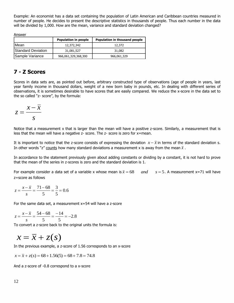
To convert a z-score back to the original units the formula is:

)(szxx

In the previous example, a z-score of 1.56 corresponds to an x-score

8.748.768)5(56.168)( szxx

And a z-score of -0.8 correspond to a x-score

13

64468)5(8.068)( szxx

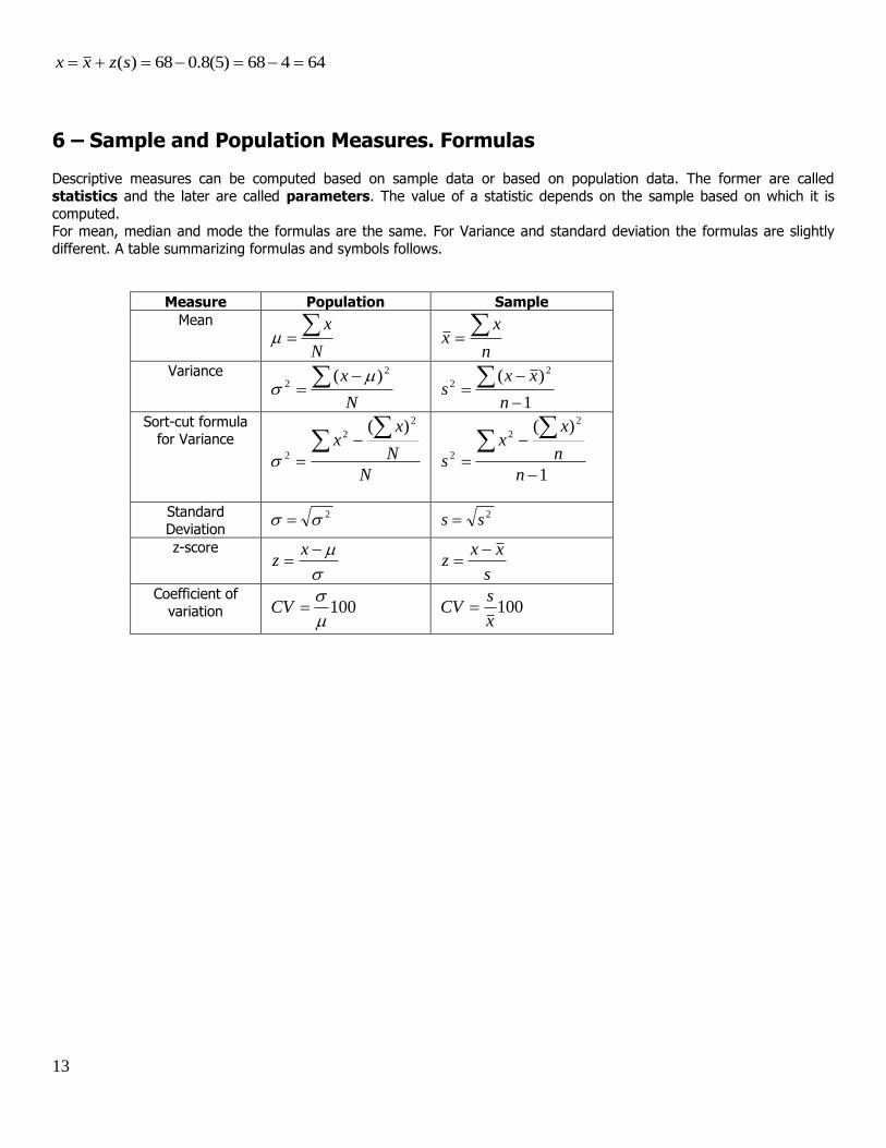
6 – Sample and Population Measures. Formulas Descriptive measures can be computed based on sample data or based on population data. The former are called

statistics and the later are called parameters. The value of a statistic depends on the sample based on which it is

computed. For mean, median and mode the formulas are the same. For Variance and standard deviation the formulas are slightly

different. A table summarizing formulas and symbols follows.

Measure Population Sample

Mean

N

x

n

xx

Variance

N

x

2

2)(

1

)( 2

2

n

xxs

Sort-cut formula for Variance

N

N

xx

2

2

2

)(

1

)( 2

2

2

n

n

xx

s

Standard

Deviation 2

2ss

z-score

xz

s

xxz

Coefficient of

variation 100

CV 100

x

sCV