Embed Size (px)
Citation preview
Design and Performance Analysis of Urban Traffic
Control Systems
Rui Sha
A thesis submitted in partial fulfilment
of the requirements for the degree of
Doctor of Philosophy
of
University College London
Department of Civil, Environmental & Geomatic Engineering
Centre for Transport Studies
University College London
December 2017


Declaration
I, Rui Sha, declare that this thesis titled, ‘Design and Performance Analysis of Urban
Traffic Control Systems’ and the work presented in it are my own. I confirm that:
• This work was done wholly or mainly while in candidature for a research
degree at University College London.
• Where I have consulted the published work of others, this is always clearly
attributed.
• Where I have quoted from the work of others, the source is always given. With
the exception of such quotations, this thesis is entirely my own work.
• I have acknowledged all main sources of help.
Signed:
Date:


If you make more roads, you will have more traffic.
by Jan Gehl

Acknowledgements
I would like to express my sincere gratitude to my supervisor Dr Andy Chow for his
academic support and insightful advices through my PhD study. His support helped
me to work productively and think a question from different perspectives. My sin-
cere thanks also go to my second supervisor Dr Tohid Erfani. I want to thank him for
his valuable opinions and encouragement. I would like to thank Dr. Kamalasudhan
Achuthan, Dr Kostantinos Ampountolas, Dr Panagiotis Angeloudis, Dr Bani Anvari
and Dr Peter Wagner for their comments on this study, and Angela Cooper for her
help on the thesis writing. I am very grateful to UCL Faculty of Engineering Sci-
ences and China Scholarships Council for funding this study.
A special thanks to my friends and UCL colleagues: Atiyeh Ardakanian, Huanfa
Chen, Fernanda Garcia Alba Garciadiego, Taha Ghasempour, Sam Ghazizadeh, Yuanyuan
Huang, David Huynh, Xianzhe Li, Kun Liu, Shuqiong Luo, Stylianos Minas, Arash
Nassirpour, Aris Pavlides, Sascha Pohoryles, Li Shuai, Palak Shukla, Peter Soi,
Alexandra Tsioulou, Fang Xu and Ying Li. They have been great companies in
the past four years and have given me fond memories.

Finally, I want to thank my family, especially my wife Lifei Liu for both her emo-
tional and academic support. I also would like to express my gratitude to my parents,
parents in law, and daughter for their love, care and joy throughout the study and life
in general.
Abstract
This study aims to investigate the design and performance of different architectures
for urban traffic control with consideration of variations and uncertainties in traffic
flow. The architectures, which ranging from centralised, semi-centralised to decen-
tralised, are applied to different road networks. Both macroscopic and microscopic
flow models are developed and used to calculate the performance of the systems.
The macroscopic model is capable of generating essential traffic dynamics, such as
traffic queues’ spillover, formation and dissipation. The control systems’ are tested
under varies traffic demand levels. The results suggest that the centralised systems
generally can outperform the decentralised systems, and the most benefit gained in
the centralised control comes from its setting of signal offsets. On the other hand,
the microscopic flow model captures the movement of each individual vehicle and
drivers' rerouting behaviour with respect to traffic conditions. The test results showed
that the drivers' response to the traffic condition can help a decentralised system per-
form as well as a centralised system. This study brings a new insight into cooperative
transport management, and contributes to the state-of-the-art of urban traffic system
design.

Contents
List of Figures i
Abbreviations vi
Notation viii
1 Introduction 1
1.1 General background . . . . . . . . . . . . . . . . . . . . . . . . . . 1
1.2 Research objectives . . . . . . . . . . . . . . . . . . . . . . . . . . 5
1.3 Report outline . . . . . . . . . . . . . . . . . . . . . . . . . . . . . 6
2 Literature review 8
2.1 Introduction . . . . . . . . . . . . . . . . . . . . . . . . . . . . . . 8
2.2 Traffic flow models . . . . . . . . . . . . . . . . . . . . . . . . . . 9
2.2.1 Microscopic flow models . . . . . . . . . . . . . . . . . . . 9
2.2.2 Macroscopic flow models . . . . . . . . . . . . . . . . . . 13
2.2.3 Discussion . . . . . . . . . . . . . . . . . . . . . . . . . . 20
2.3 Urban traffic control systems . . . . . . . . . . . . . . . . . . . . . 21
2.3.1 Fixed-time control systems . . . . . . . . . . . . . . . . . . 23
2.3.2 Traffic-responsive control systems . . . . . . . . . . . . . . 26
2.3.3 Discussion . . . . . . . . . . . . . . . . . . . . . . . . . . 30
2.4 Optimisation methods for signal control . . . . . . . . . . . . . . . 32
2.4.1 Formulation of the traffic signal control problem . . . . . . 32
2.4.2 Exact methods . . . . . . . . . . . . . . . . . . . . . . . . 39
2.4.3 Heuristic methods . . . . . . . . . . . . . . . . . . . . . . 40
2.4.4 Discussion . . . . . . . . . . . . . . . . . . . . . . . . . . 49
3 Analysis of urban traffic control systems 52
3.1 Introduction . . . . . . . . . . . . . . . . . . . . . . . . . . . . . . 52
3.2 Centralised control . . . . . . . . . . . . . . . . . . . . . . . . . . 53
3.2.1 Brute Force Approach . . . . . . . . . . . . . . . . . . . . 53
3.2.2 Genetic Algorithm . . . . . . . . . . . . . . . . . . . . . . 56
3.3 Semi-decentralised control . . . . . . . . . . . . . . . . . . . . . . 60
3.3.1 TUC system . . . . . . . . . . . . . . . . . . . . . . . . . 60
3.3.2 Hybrid system . . . . . . . . . . . . . . . . . . . . . . . . 68
3.4 Decentralised control . . . . . . . . . . . . . . . . . . . . . . . . . 70
3.4.1 Max-pressure controller . . . . . . . . . . . . . . . . . . . 70
3.5 Summary . . . . . . . . . . . . . . . . . . . . . . . . . . . . . . . 74
4 Comparing centralised and decentralised traffic control under a macro-
scopic flow model 76
4.1 Introduction . . . . . . . . . . . . . . . . . . . . . . . . . . . . . . 76
4.2 One-way arterial network . . . . . . . . . . . . . . . . . . . . . . . 77
4.2.1 Network Configurations . . . . . . . . . . . . . . . . . . . 77
4.2.2 Settings of the test control systems . . . . . . . . . . . . . . 80
4.2.3 Test results . . . . . . . . . . . . . . . . . . . . . . . . . . 81
4.3 Two-way arterial network . . . . . . . . . . . . . . . . . . . . . . . 87
4.3.1 Network configurations . . . . . . . . . . . . . . . . . . . . 87
4.3.2 Test results . . . . . . . . . . . . . . . . . . . . . . . . . . 88
4.4 Grid network . . . . . . . . . . . . . . . . . . . . . . . . . . . . . 91
4.4.1 Network configurations . . . . . . . . . . . . . . . . . . . . 91
4.4.2 Test results . . . . . . . . . . . . . . . . . . . . . . . . . . 91
4.5 Decentralised systems with hill climbing offset controller . . . . . . 95
4.6 Summary . . . . . . . . . . . . . . . . . . . . . . . . . . . . . . . 103
5 Comparing centralised and decentralised traffic control under a micro-
scopic flow model with traffic rerouting 105
5.1 Introduction . . . . . . . . . . . . . . . . . . . . . . . . . . . . . . 105
5.2 Simulation of urban mobility - SUMO . . . . . . . . . . . . . . . . 106
5.2.1 Traffic dynamics . . . . . . . . . . . . . . . . . . . . . . . 107
5.2.2 Dynamic rerouting algorithm . . . . . . . . . . . . . . . . . 108
5.2.3 Converting CTM settings into SUMO . . . . . . . . . . . . 110
5.2.4 Implementation of traffic signals . . . . . . . . . . . . . . . 115
5.3 One-way arterial network . . . . . . . . . . . . . . . . . . . . . . . 118
5.3.1 Network configurations . . . . . . . . . . . . . . . . . . . . 118
5.3.2 Settings of the test control systems . . . . . . . . . . . . . . 120
5.3.3 Performance criteria . . . . . . . . . . . . . . . . . . . . . 121
5.3.4 Test results . . . . . . . . . . . . . . . . . . . . . . . . . . 123
5.4 Grid network . . . . . . . . . . . . . . . . . . . . . . . . . . . . . 126
5.4.1 Test under different traffic saturation levels . . . . . . . . . 126
5.4.2 Test under different traffic spatial distributions . . . . . . . 133
5.4.3 Test on rerouting compliance rate . . . . . . . . . . . . . . 138
5.4.4 Test on a road incident scenario . . . . . . . . . . . . . . . 141
5.4.5 Test on London road network . . . . . . . . . . . . . . . . 147
5.4.6 An adaptive TUC system with rerouting control . . . . . . . 151
5.5 Summary . . . . . . . . . . . . . . . . . . . . . . . . . . . . . . . 156
6 Conclusions and outlook 157
6.1 Thesis overview . . . . . . . . . . . . . . . . . . . . . . . . . . . . 157
6.2 Contributions . . . . . . . . . . . . . . . . . . . . . . . . . . . . . 160
6.3 Future work . . . . . . . . . . . . . . . . . . . . . . . . . . . . . . 162
Appendix A Genetic Algorithm 163
Appendix B TUC: split control 170
References 177
List of Figures
1.1 The urban traffic control system monitors more than 450 of the in-
tersections in Nottingham (Source: World Highways, 2010) . . . . . 2
1.2 An example of urban traffic control system: SCOOT . . . . . . . . 3
1.3 Different control structures of traffic control systems . . . . . . . . 4
2.1 An example of perception threshold of the psycho-physical model . 13
2.2 Fundamental diagrams . . . . . . . . . . . . . . . . . . . . . . . . 15
2.3 Different phases of a signalised intersection . . . . . . . . . . . . . 22
2.4 Different stages of a signalised intersection . . . . . . . . . . . . . 23
2.5 An illustration of signal settings . . . . . . . . . . . . . . . . . . . 23
2.6 Architecture of a SCATS system . . . . . . . . . . . . . . . . . . . 28
2.7 Locations of MOVA system's loop detectors . . . . . . . . . . . . . 30
2.8 Four signal plans with different offset settings . . . . . . . . . . . . 39
2.9 A flowchart of Genetic Algorithm . . . . . . . . . . . . . . . . . . 42
2.10 A flowchart of Ant Colony Optimisation . . . . . . . . . . . . . . . 44
2.11 A flowchart of Tabu Search . . . . . . . . . . . . . . . . . . . . . . 46
2.12 A flowchart of Simulated Annealing . . . . . . . . . . . . . . . . . 48
i
3.1 An example of feasible values of the green splits . . . . . . . . . . 55
3.2 A set of network signal plans for the brute force approach . . . . . . 55
3.3 A chromosome structure of a network signal plan . . . . . . . . . . 58
3.4 GA's crossover process . . . . . . . . . . . . . . . . . . . . . . . . 59
3.5 An illustration of offset control . . . . . . . . . . . . . . . . . . . . 66
3.6 Offset control with residue queues . . . . . . . . . . . . . . . . . . 67
4.1 Test one-way arterial network . . . . . . . . . . . . . . . . . . . . . 79
4.2 Average network delays on the one-way arterial . . . . . . . . . . . 83
4.3 Green splits at Node 3 over different γ on the one-way arterial network 84
4.4 Offsets at Node 3 over different γ on the one-way arterial network . 85
4.5 Density plot at γ = 0.9 on the one-way arterial network controlled by
the brute force approach . . . . . . . . . . . . . . . . . . . . . . . 86
4.6 Test two-way arterial network . . . . . . . . . . . . . . . . . . . . 88
4.7 Average network delays on the two-way arterial . . . . . . . . . . . 89
4.8 Green splits at Node 3 over different γ on the two-way arterial network 90
4.9 Offsets at Node 3 over different γ on the two-way arterial network . 90
4.10 Test grid network . . . . . . . . . . . . . . . . . . . . . . . . . . . 92
4.11 Average network delays on the grid network . . . . . . . . . . . . . 93
4.12 Green split at Node 4 over different γ on the grid network . . . . . . 94
4.13 Offsets at Node 4 over different γ on the grid network . . . . . . . . 94
4.14 A flowchart of hill climbing offset control . . . . . . . . . . . . . . 99
4.15 A sensitivity analysis of hill climbing step sizes . . . . . . . . . . . 100
4.16 Network delays in the one-way arterial network with hill climbing
offset controller . . . . . . . . . . . . . . . . . . . . . . . . . . . . 101
4.17 Network delays in the two-way arterial network with hill climbing
offset controller . . . . . . . . . . . . . . . . . . . . . . . . . . . . 102
4.18 Network delays in the grid network with hill climbing offset controller102
5.1 An illustration of rerouting on a road network . . . . . . . . . . . . 110
5.2 Arrival and departure curves of CTM and SUMO when undersaturated112
5.3 Arrival and departure curves of CTM and SUMO when oversaturated 113
5.4 Network delay of CTM and SUMO when undersaturated . . . . . . 113
5.5 Network delay of CTM and SUMO when oversaturated . . . . . . . 114
5.6 Traffic control interface of SUMO . . . . . . . . . . . . . . . . . . 116
5.7 An example of the signal plan in SUMO . . . . . . . . . . . . . . . 117
5.8 Test one-way arterial network used in SUMO . . . . . . . . . . . . 118
5.9 An example of a green band formed on an arterial network . . . . . 123
5.10 Average network delay of the one-way arterial network over γ . . . 125
5.11 Average green bandwidth of the one-way arterial network over γ . . 125
5.12 Test three by three grid network used in SUMO . . . . . . . . . . . 129
5.13 Average network delay of the three by three grid network over γ
without rerouting . . . . . . . . . . . . . . . . . . . . . . . . . . . 129
5.14 Average green bandwidth of the three by three grid network over γ
without rerouting . . . . . . . . . . . . . . . . . . . . . . . . . . . 130
5.15 Average queue length at intersections of the three by three grid net-
work (γ = 0.9, σ = 0.3 without rerouting) . . . . . . . . . . . . . . 130
5.16 Average network delay of the three by three grid network over γ with
rerouting . . . . . . . . . . . . . . . . . . . . . . . . . . . . . . . . 131
5.17 Average green bandwidth of the three by three grid network over γ
with rerouting . . . . . . . . . . . . . . . . . . . . . . . . . . . . . 131
5.18 Average queue length at intersections of the three by three grid net-
work (γ = 0.9, σ = 0.3 with rerouting) . . . . . . . . . . . . . . . . 132
5.19 Average network delay of the three by three grid network over σ
without rerouting . . . . . . . . . . . . . . . . . . . . . . . . . . . 134
5.20 Average green bandwidth of the three by three grid network over σ
without rerouting . . . . . . . . . . . . . . . . . . . . . . . . . . . 135
5.21 Average queue length at intersections of the three by three grid net-
work (γ = 0.7, σ = 0.7 without rerouting) . . . . . . . . . . . . . . 135
5.22 Average network delay of the three by three grid network over σ
with rerouting . . . . . . . . . . . . . . . . . . . . . . . . . . . . . 136
5.23 Average green bandwidth of the three by three grid network over σ
with rerouting . . . . . . . . . . . . . . . . . . . . . . . . . . . . . 136
5.24 Average queue length at intersections of the three by three grid net-
work (γ = 0.7, σ = 0.7 with rerouting) . . . . . . . . . . . . . . . . 137
5.25 Average network delay of the three by three grid network over dif-
ferent rerouting compliance rate σ = 0.3 . . . . . . . . . . . . . . . 139
5.26 Average network delay of the three by three grid network over dif-
ferent rerouting compliance rate σ = 0.6 . . . . . . . . . . . . . . . 140
5.27 Average network delay of the three by three grid network over dif-
ferent rerouting compliance rate σ = 0.9 . . . . . . . . . . . . . . . 140
5.28 Test five by five grid network . . . . . . . . . . . . . . . . . . . . . 143
5.29 Network delay of the road incident scenario without rerouting . . . 144
5.30 Network delay of the road incident scenario with rerouting . . . . . 144
5.31 Average network bandwidth of the road incident scenario without
rerouting . . . . . . . . . . . . . . . . . . . . . . . . . . . . . . . . 145
5.32 Average network bandwidth of the road incident scenario with rerout-
ing . . . . . . . . . . . . . . . . . . . . . . . . . . . . . . . . . . . 145
5.33 Change of network queue distribution without rerouting . . . . . . . 146
5.34 Change of network queue distribution with rerouting . . . . . . . . 146
5.35 London Bloomsbury area test network . . . . . . . . . . . . . . . . 149
5.36 An example of measured traffic flow data . . . . . . . . . . . . . . 150
5.37 Test results at the Bloomsbury network . . . . . . . . . . . . . . . . 150
5.38 Network delay of three TUC systems over γ without rerouting . . . 152
5.39 Network delay of three TUC systems over γ with rerouting . . . . . 153
5.40 Improvement of network delay by rerouting over γ . . . . . . . . . 153
5.41 Network delay of three TUC systems over σ without rerouting . . . 154
5.42 Network delay of three TUC systems over σ with rerouting . . . . . 154
5.43 Improvement of network delay by rerouting over σ . . . . . . . . . 155

Abbreviations
BF Brute Force
CTM Cell Transmission Model
FIT Fitness
GA Genetic Algorithm
GHR Gazis-Herman-Rothery
HC Hill-Climbing
HJB Hamilton-Jacobi-Bellman
LQR Linear-Quadratic Regulator
LWR Lighthill and Whitham-Richards
MP Max-Pressure
SUMO Simulation of Urban Mobility
TND Total Network Delay
TRANSYT Traffic Network Study Tool
TUC Traffic-responsive Urban Control
vi

VDT Vehicle Distance Travelled
VHT Vehicle Hours Travelled
VISSIM Verkehr In StÃd’dten - SIMulationsmodel
Notation
C cycle time [sec]
C a set of all cells in a network
CN nominal cycle time [sec]
Cmin minimum cycle time [sec]
Cmax maximum cycle time [sec]
CI converted integer cycle time [sec]
c cell (or road section) index
cl , cm relaxation constant and anticipation constant in
Payne's second order flow model
cs magnification parameter of performance differences
between chromosomes
cv, cκ sensitivity parameters in METANET flow model
cα a fundamental relationship parameter in METANET
flow model
cβ a sensitivity coefficient of a stimulus-response
model
viii
d standstill distance between two successive vehicles [m]
dmin minimum distance between two successive vehicles [m]
dcrit critical distance between two successive vehicles [m]
G a set of green phases
GI converted integer green split [sec]
g green split [sec]
gN nominal green split [sec]
gmin minimum green split [sec]
g∗ scaled green split [sec]
g gravitational acceleration [m2/sec]
H sum of demand to saturation flow ratio for all signal
stages
h demand to saturation flow ratio
I a set of all network roads (links)
Iin a set of all the inflow roads (links) to an intersection
(node)
Iout a set of all the outflow roads (links) to an intersection
(node)
i road (link) index
j intersection index
Kc the parameter of cycle time control intensity
k cycle index
L control gain matrix
LT lost time [sec]
lcell cell length [m]
llink link length [m]
lveh vehicle length [m]
lveh mean vehicle length [m]
m vehicle index
n intersection (node) index
o offset [sec]
o∗ optimal offset [sec]
Q maximum flow or saturation flow [veh/hr]
q traffic flow rate [veh/hr]
R a set of red phases
R a set of routes
T time period
t time step index
U a set of signal timing plans
u average road (link) travel time
v vehicle speed [m/sec]
vdes vehicle's desired speed [m/sec]
vfinal vehicle's final speed [m/sec]
vmax vehicle's maximum speed [m/sec]
vsafe vehicle's safe speed [m/sec]
w shockwave speed

x road (link) queue length [veh]
xmax road (link) capacity [veh]
α vehicle acceleration or deceleration rate [m2/sec]
γ degree of congestion
ε drivers' imperfection factor
ζ turning ratio
η sensitivity parameter of pressure
Θ a set of all stages
θ stage index
ι stage switch indicator
Λ traffic demand profile
λ demand magnitude parameter [veh/hr]
µ a friction coefficient between vehicle and road sur-
face
ξ ratio of queue length to the road (link) queue capac-
ity
ρ traffic density, the number of vehicles at a unit length
of a road
[veh/m]
ρcrit critical density [veh/m]
ρjam jam density [veh/m]
τ driver's reaction time
σ traffic spatial distribution parameter
υ average traffic speed [m/sec]

υf free flow speed [m/sec]
υcrit critical speed [m/sec]
υequal an equilibrium speed for high order flow model [m/sec]
χ vehicle location
ψ pressure in Max-pressure control [veh2/sec]
Chapter 1
Introduction
1.1 General background
According to the United Nations' statistics record [1], 54 percent of the world pop-
ulation live in cities. This ratio is projected to reach to 66% by 2050, where it was
only 34% in the 1960s. The continuous growth in the urban population will lead to
the increase in traffic volume. As reported by the Department of Transport, the traf-
fic across the UK will rise 19%-55% during the period from 2010 to 2040 [2]. The
growth of traffic challenges the operation of existing urban transport infrastructure
and aggravates the traffic congestion problem in large cities like London. Traffic
congestion not only has negative impacts on economic growth and social develop-
ment, but also has severe effects on citizens'daily activities. The traffic information
company INRIX found the time wasted in traffic congestion over 2016 is 73.4 hours
in London, 65.3 hours in Paris and 39.4 hours in Manchester per passenger per year
[3].
1
Chapter 1. Introduction
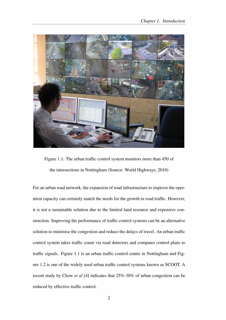
Figure 1.1: The urban traffic control system monitors more than 450 of
the intersections in Nottingham (Source: World Highways, 2010)
For an urban road network, the expansion of road infrastructure to improve the oper-
ation capacity can certainly match the needs for the growth in road traffic. However,
it is not a sustainable solution due to the limited land resource and expensive con-
struction. Improving the performance of traffic control systems can be an alternative
solution to minimise the congestion and reduce the delays of travel. An urban traffic
control system takes traffic count via road detectors and computes control plans to
traffic signals. Figure 1.1 is an urban traffic control centre in Nottingham and Fig-
ure 1.2 is one of the widely used urban traffic control systems known as SCOOT. A
recent study by Chow et al [4] indicates that 25%-30% of urban congestion can be
reduced by effective traffic control.
2
Chapter 1. Introduction
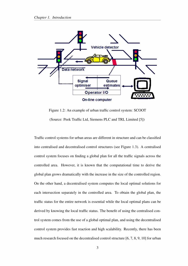
Figure 1.2: An example of urban traffic control system: SCOOT
(Source: Peek Traffic Ltd, Siemens PLC and TRL Limited [5])
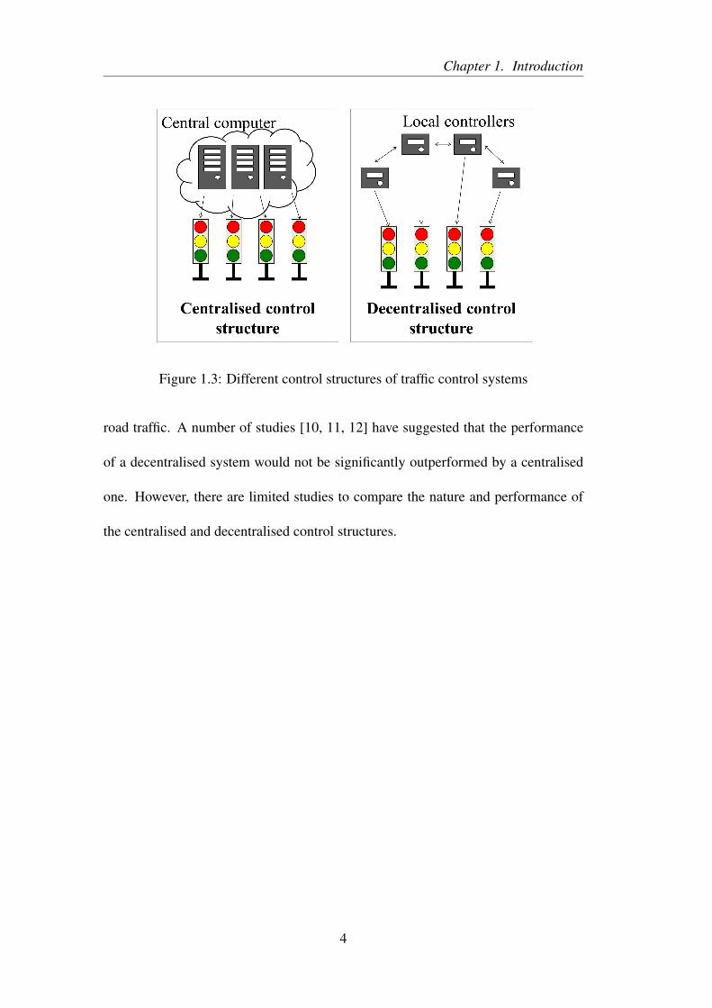
Traffic control systems for urban areas are different in structure and can be classified
into centralised and decentralised control structures (see Figure 1.3). A centralised
control system focuses on finding a global plan for all the traffic signals across the
controlled area. However, it is known that the computational time to derive the
global plan grows dramatically with the increase in the size of the controlled region.
On the other hand, a decentralised system computes the local optimal solutions for
each intersection separately in the controlled area. To obtain the global plan, the
traffic status for the entire network is essential while the local optimal plans can be
derived by knowing the local traffic status. The benefit of using the centralised con-
trol system comes from the use of a global optimal plan, and using the decentralised
control system provides fast reaction and high scalability. Recently, there has been
much research focused on the decentralised control structure [6, 7, 8, 9, 10] for urban
3
Chapter 1. Introduction
Figure 1.3: Different control structures of traffic control systems
road traffic. A number of studies [10, 11, 12] have suggested that the performance
of a decentralised system would not be significantly outperformed by a centralised
one. However, there are limited studies to compare the nature and performance of
the centralised and decentralised control structures.
4
Chapter 1. Introduction
1.2 Research objectives
This study focuses on the performance difference between centralised and decen-
tralised control systems for urban traffic management. The performance difference
can provide important insights and guidance on how to design the decentralised con-
trol system and bridge the gap with the centralised system. The main objectives of
this study are shown as follows:
1. Review the control structures of existing urban traffic control systems and
identify the differences in design between centralised and decentralised ones.
2. Build a test platform which can evaluate the performance of traffic control
systems.
3. Compare the performances between the centralised and decentralised traffic
control systems under different traffic demand with variation and uncertainty.
4. Propose feasible methods to bridge the efficiency gap between the centralised
and decentralised systems based on the findings of the previous objective.
5
Chapter 1. Introduction
1.3 Report outline
The remainder of this report is organised as follows:
Chapter 2 is a review of different types of traffic flow models, urban control systems
and traffic signal optimisation techniques. A traffic flow model is a mathematical
representation of traffic dynamics, and is a common tool used for traffic modelling
and forecasting. The review of the flow model discusses the features of each flow
model and determines the ones which are appropriate to use for this study. The re-
view of the urban traffic control system explains the developments of the system and
different control structures. The review of the optimisation techniques discussed the
use of exact methods and heuristic methods in traffic signal control problems.
Chapter 3 analyses the control principles of selected centralised and decentralised
traffic control systems. Two searching techniques are used to derive global signal
plans which represent the centralised systems. TUC and Hybrid systems are semi-
decentralised systems, where parts of the signal plan are derived from decentralised
controllers. Max-pressure controller is a decentralised system which only uses local
traffic information to operate traffic signals.
Chapter 4 investigates the performance of the control systems. A macroscopic flow
model is used to describe the traffic dynamics. The experiment is carried out in three
networks with a range of traffic demands from undersaturation to oversaturation.
6
Chapter 1. Introduction
Chapter 5 investigates the performance of the control systems at a deeper level. The
movement of individual vehicles are simulated by a microscopic flow model, and
drivers' rerouting behaviour respecting real-time traffic condition is captured. The
experiment is performed on four networks with different demand levels and spatial
distributions.
Chapter 6 is a conclusion of the thesis and outlines the future work of this study.
7
Chapter 2
Literature review
2.1 Introduction
This chapter is a review of traffic flow models, traffic control systems, and traffic
signal optimisation methods . A traffic flow model is an essential tool for transport
planning and operation, since it is a mathematical representation of traffic dynamics
and an analytic expression of traffic forecast. Traffic control systems have been used
as the main measure to improve traffic flow in urban road networks. They prevent
the traffic movement conflicts at intersections and give appropriate traffic signals to
reduce travel delays. Optimisation methods show the insight of the traffic control
systems and how traffic signal plans are derived. Section 2.2 reviews different types
of traffic flow models, Section 2.3 presents the development made in urban traffic
control systems and Section 2.4 discusses the differences between various imple-
mented optimisation methods.
8
Chapter 2. Literature review
2.2 Traffic flow models
The traffic flow model is a mathematical description of traffic dynamics. It is used
to analyse traffic phenomena and to provide efficient traffic operations. The devel-
opment of the flow model has been carried out for half a century, hence, there exist
a wide range of models. The level of detail (microscopic or macroscopic) is com-
monly used as a criterion to categorise traffic flow models. This section reviews
microscopic and macroscopic traffic flow models and discusses their features to de-
termine which ones are suitable to use in this study.
2.2.1 Microscopic flow models
A microscopic traffic flow model considers detailed movements of each individ-
ual vehicle, such as lane change, acceleration and other drivers' behaviour. As a
modelled vehicle in the flow model has a strong relation to its front vehicle, the mi-
croscopic flow model is also known as the car-following model. Some main types
of car-following models are: the stimulus-response model, safety-distance model,
and psycho-physical model [13]. They base on different assumptions of driving be-
haviours.
Stimulus-response models
The stimulus-response models describe the response of a driver as a product of a
stimulus and the driver's sensitivity to the stimulus. A general form of the stimulus-
response model suggested by Chandler et al [14] is:
9
Chapter 2. Literature review
αm+1(t +1) = cβ [vm(t)− vm+1(t)] (2.1)
cβ is a sensitivity coefficient of vehicle m to the stimulus, which is the difference
in speeds vm(t)− vm+1(t) between the successive vehicles m and m+1. The accel-
eration (deceleration) α of the follower vehicle m+1 is a response to the stimulus.
The response at a time step t +1 is calculated from the stimulus at time step t, since
there is a time lag between the response and the stimulus. As the driver may become
more sensitive to the stimulus when vehicles are close to each other, Gazis et al [15]
modified Equation 2.1 to:
αm+1(t +1) =cβ
χm(t)−χm+1(t)[vm(t)− vm+1(t)] (2.2)
The expression of the sensitivity becomes tocβ
χm(t)−χm+1(t), which is affected by the
distances between the successive vehicles m and m+1. Equation 2.2 is subsequently
generalised as:
αm+1(t +1) =cβ vm(t +1)c
l
[χm(t)−χm+1(t)]cm[vm(t)− vm+1(t)] (2.3)
Equation 2.3 is known as the Gazis-Herman-Rothery (GHR) model [16], and the
parameters cl and cm are calibrated with fields data in several studies, such as [17]
and [18]. Although the stimulus-response model has been proposed since the late
10
Chapter 2. Literature review
1950s, it had been used less frequently until the mid-1990s due to the findings on the
parameter values contradict with each other [19].
Safety-distance models
The second type of car-following models is the safety-distance model. Different
from the stimulus-response model, a safety-distance model is based on the assump-
tion that successive vehicles maintain a safe distance with each other to avoid colli-
sion. The early safety-distance model proposed by Pipe [20] expresses the location
of two successive vehicle m and m+1 as:
χm = χm+1 +d + lvehm + τvm+1 (2.4)
In Equation 2.4, d is the standstill distance between the vehicles, lveh is the vehicle
length and τvn+1 represents the travel distance. The travel distance is calculated as
the product of the driver's reaction time τ and its travel speed vm+1 of the vehicle
m+ 1. The whole part of d + lvehm + τvm+1 forms the safe distance between the ve-
hicles m and m+ 1. Comparing to the traffic data measured from field, the Pipe's
model has less headway distance when vehicles travel at the speed close to mini-
mum or maximum allowed speed [21]. Leutzbach [22] modifies the Pipe's model by
introducing a breaking distance v2m+1
2µg , and the new expression is shown as:
χm = χm+1 + lvehm + τvm+1 +
v2m+1
2µ g(2.5)
11
Chapter 2. Literature review
where the µ is friction coefficient between vehicle and road surface and g stands for
gravitational acceleration rate.
One development in the safety-distance model includes a time lag between the change
in space headway with the front vehicle and the follower vehicle's reaction [23]. This
model has been developed into a hybrid flow model [24] by combining with the LWR
model (introduced in Section 2.2.2).
Psycho-physical models
The psycho-physical model is another branch of the car-following models and are
also known as the action point model. It is similiar to safety-distance model, but
with a more detailed description on drivers' behaviour. In previous mentioned mi-
croscopic models, drivers strictly react to the headway change χm− χm+1 and rela-
tive speed change vm− vm+1 which are not the same in real life. A driver will not
actively react to the front vehicle when the two vehicles are far apart. If the two
vehicles are close to each other, the motion will be small for a driver to respond to
changes in relative speed or headway so that the driver may not react as well. The
first psycho-physical model is proposed by Wiedemann [25] and is the foundation
of the widely used microscopic simulation software VISSIM [26]. In Wiedemann's
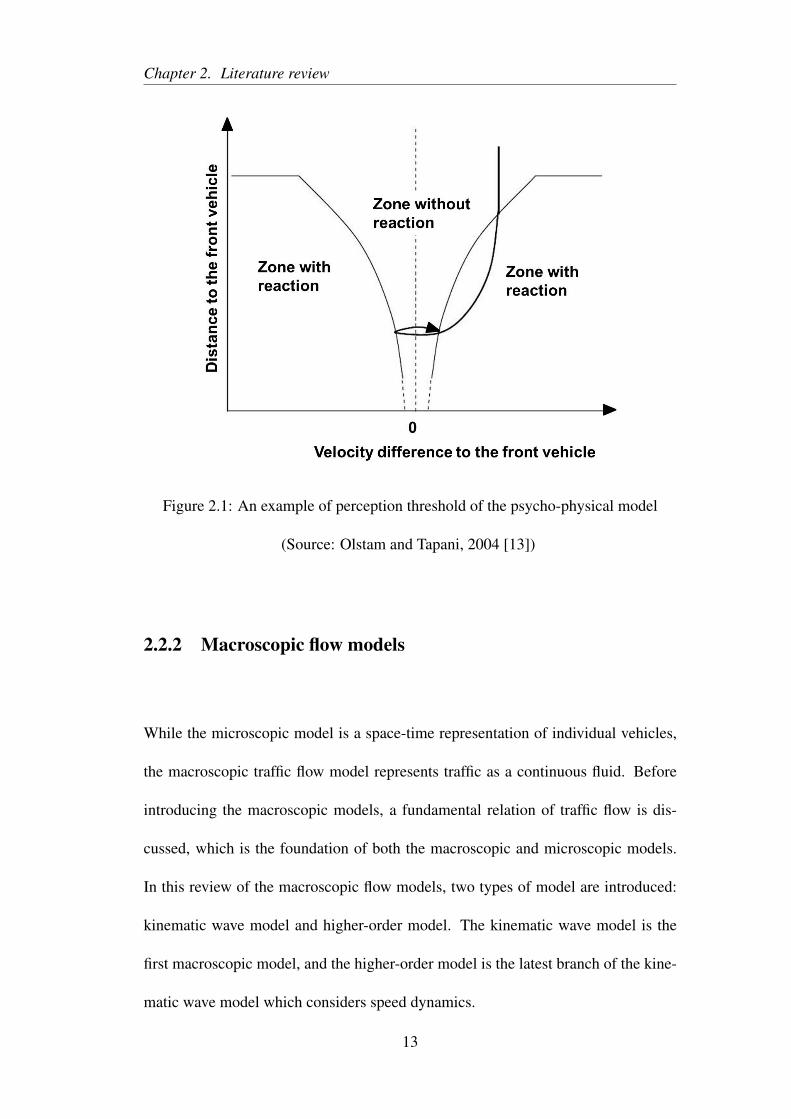
model, perception thresholds are introduced (see Figure 2.1) to determine whether
drivers will obey the car-following rules or not.
12
Chapter 2. Literature review
Figure 2.1: An example of perception threshold of the psycho-physical model
(Source: Olstam and Tapani, 2004 [13])
2.2.2 Macroscopic flow models
While the microscopic model is a space-time representation of individual vehicles,
the macroscopic traffic flow model represents traffic as a continuous fluid. Before
introducing the macroscopic models, a fundamental relation of traffic flow is dis-
cussed, which is the foundation of both the macroscopic and microscopic models.
In this review of the macroscopic flow models, two types of model are introduced:
kinematic wave model and higher-order model. The kinematic wave model is the
first macroscopic model, and the higher-order model is the latest branch of the kine-
matic wave model which considers speed dynamics.
13
Chapter 2. Literature review
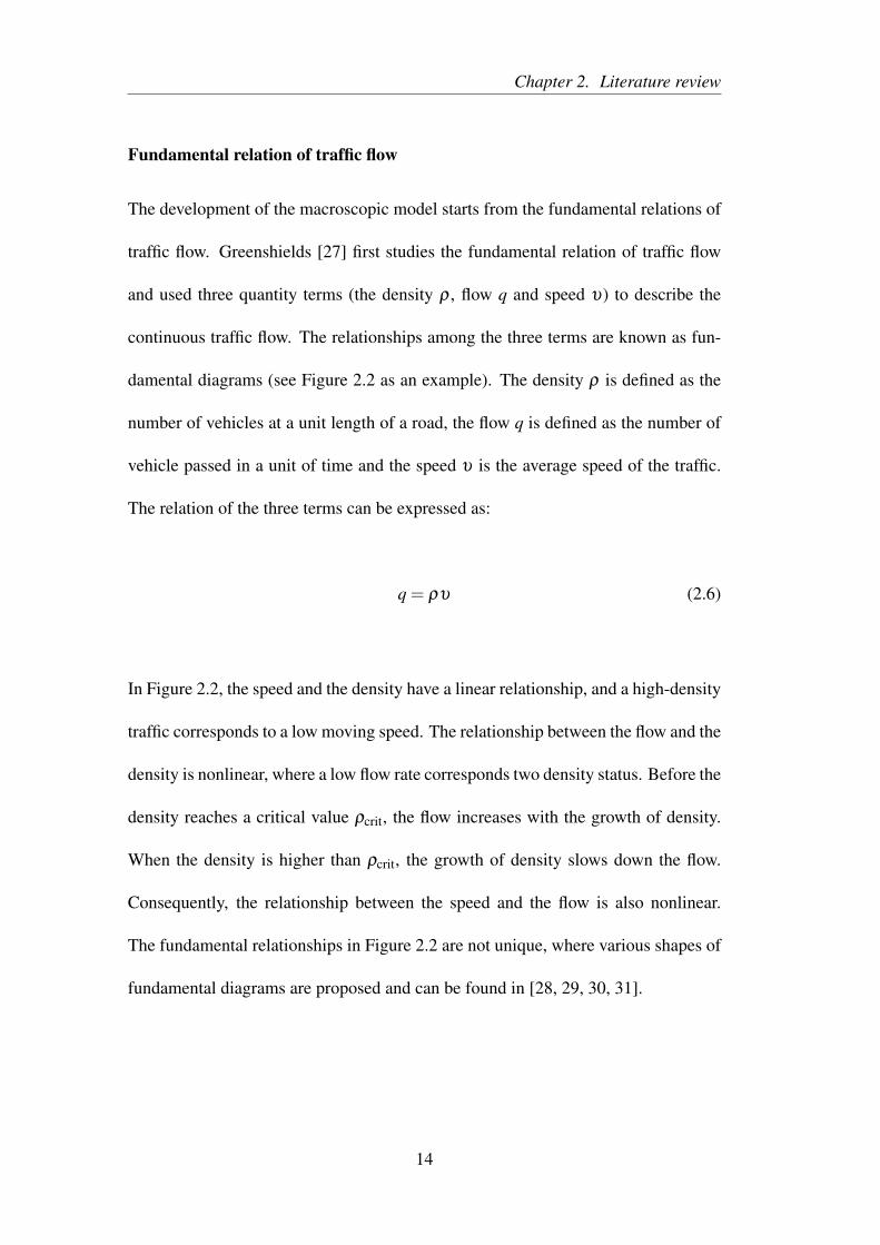
Fundamental relation of traffic flow
The development of the macroscopic model starts from the fundamental relations of
traffic flow. Greenshields [27] first studies the fundamental relation of traffic flow
and used three quantity terms (the density ρ , flow q and speed υ) to describe the
continuous traffic flow. The relationships among the three terms are known as fun-
damental diagrams (see Figure 2.2 as an example). The density ρ is defined as the
number of vehicles at a unit length of a road, the flow q is defined as the number of
vehicle passed in a unit of time and the speed υ is the average speed of the traffic.
The relation of the three terms can be expressed as:
q = ρυ (2.6)
In Figure 2.2, the speed and the density have a linear relationship, and a high-density
traffic corresponds to a low moving speed. The relationship between the flow and the
density is nonlinear, where a low flow rate corresponds two density status. Before the
density reaches a critical value ρcrit, the flow increases with the growth of density.
When the density is higher than ρcrit, the growth of density slows down the flow.
Consequently, the relationship between the speed and the flow is also nonlinear.
The fundamental relationships in Figure 2.2 are not unique, where various shapes of
fundamental diagrams are proposed and can be found in [28, 29, 30, 31].
14
Chapter 2. Literature review
Figure 2.2: Fundamental diagrams
Kinematic wave models
The first macroscopic flow model is proposed by Lighthill, Whitham and Richards
[32, 33], which is known as the LWR model or kinematic wave model. The LWR
model is a conservation law where no vehicle can be created or removed within a
closed road section. Any changes in traffic (∆q and ∆ρ) have to be the same during
time interval ∆t in the closed road section. The following expression is found for the
conservation law:
∆ρ
∆t+
∆q∆χ
= 0 (2.7)
∆χ is the length of the road section. When ∆χ and ∆t approach to 0, Equation 2.7
converts to the general expression of the LWR model:
∂ρ
∂ t+
∂q∂ χ
= 0 (2.8)
15
Chapter 2. Literature review
In order to solve the LWR model, several approaches have been proposed such as:
Godunov method [34] and Cell Transmission Model (CTM) [31]. The CTM is one
of the most popular methods, which dicretise each road into a collection of cells.
According to the conservation law (Equation 2.8), the traffic density ρ of each cell i
at time t can be expressed as:
ρc(t +1) = ρc(t)+∆t
lcellc
[qc−1(t)−qc(t)] , (2.9)
where qc(t) is the outflow from cell c. Cell c− 1 is the upstream cell, where traffic
flows from cell c− 1 into cell c. ∆t is one time step and lcellc is the length of cell c.
The step size ∆t has to satisfy ∆t ≤min(lcell
υ), which means the traffic can not travel
more than one cell per time step.
CTM has a piecewise linear relationship with the traffic flow q and density ρ be-
tween each pair of successive cells (c,c+ 1). The maximum flow rate (saturation
flow rate) for each cell is Q, and the maximum density (jam density) of each cell is
ρjam. When there is no congestion, traffic moves through cells at a maximum speed
(free flow speed). With the piecewise linear relationship, the outflow qc(t) from cell
c to its downstream c+1 is determined as:
qc(t) = min{
υcρc(t),Qc,Qc+1,wc+1[ρjam,c+1−ρc+1(t)
]}, (2.10)
where w is a shockwave speed which refers to the backward propagation speed of
16
Chapter 2. Literature review
traffic. Equation 2.10 can be considered as an expression of the triangular flow-
density relationship. In addition, the effect of traffic signals is formulated as a binary
variable at cell c:
Qc(t) =
Qc, t ∈G
0, t ∈ R
(2.11)
G and R stand of the green and red phases. The setting of G and R use a timing plan
derived from the signal control system.
The LWR model is sufficient to describe the basic flow dynamics such as formation
and dissipation of traffic congestion. However, due to its simplicity, LWR has several
issues such as the limitations in describing vehicle's speed dynamics and formulating
the capacity drop phenomenon. The solution to address the dynamics of vehicle's
speed is the higher-order model.
Higher-order models
Higher-order models are developed to overcome the limitation of the LWR model in
mean speed dynamics. The LWR flow model contains one partial differential equa-
tion. Payne [35] proposed a second order flow model which contains the LWR's
partial differential equation (conservation of vehicles) Equation 2.8 and another par-
tial differential equation to describe mean speed dynamics. In the Payne's model, the
average speed of traffic on a road section is not only affected by the traffic density
but also by the neighbour traffic conditions. The expression of mean speed dynamics
17
Chapter 2. Literature review
in Payne's model is as follows:
∂υ
∂ t+υ
∂υ
∂ χ=
(υequal(ρ)−υ)
cl− c2
mρ
∂ρ
∂ χ(2.12)
where υequal(ρ) is an equilibrium speed associated with density ρ . cl and cm are
relaxation constant and anticipation constant respectively. The term υ∂υ
∂ χstands for
the convection of traffic. Given a road section where vehicles are travel from its up-
stream road section, the average speeds of the two sections may not be the same. In
this case, the vehicles have to accelerate or decelerate ∂v∂x to adapt the traffic speed.
In terms of the (υequal(ρ)−υ)c1
, this is a relaxation term where the vehicles will try to
reach the equilibrium speed υequal of the road section. The last term c22
ρ
∂ρ
∂ χrepresents
drivers' anticipation to their downstream road section. When the density ρ at the
downstream road section is higher, the driver will anticipate to slow down.
A METANET [36] is a popular software used Payne's model for motorway mod-
elling. It separates each road into a group of sections, and the length of each road
section is l. Both fundamental relation of traffic flow (Equation 2.6) and conservation
law (Equation 2.9) are considered. The mean speed dynamics of the METANET's
model is as follows:
υc(t +1) =υc(t)+∆tτ[υequal,c(ρc(t))−υc(t)]−
∆tl
υc(t)[υc−1(t)−υc(t)]
− cv∆tτl
ρc+1(t)−ρc(t)ρc(t)+ cκ
(2.13)
The relaxation term ∆tτ[υequal,c(ρc(t))−υc(t)] describes the behaviour of the drivers.
18
Chapter 2. Literature review
Drivers will try to achieve the equilibrium speed υequal,c(ρc(t)) of the road section.
τ is the reaction time for drivers to realise the equilibrium speed of the road section,
and when τ value is small the drivers can response quicker. The convection term
∆tl υc(t)[υc−1(t)−υc(t)] captures the impact of the driver's speed change from the
upstream road section c−1. The last term cv∆tτl
ρc+1(t)−ρc(t)ρc(t)+cκ
is the anticipation term to
consider drivers' speed change with respect to downstream road density. cv and cκ
are sensitivity parameters and they allow the model to be more sensitive to medium
or high density. The equilibrium mean speed in the relaxation term is derived from:
υequal,c[(ρc(t))] = υf,cexp(− 1cα
(ρc(t)ρcrit
)cα ) (2.14)
where υf,c is the free flow speed of road section c. cα is a parameter which helps to
form a non-linear fundamental relationship between the density and the mean speed.
Apart from the second order model, the higher order model can be further extended
to a third order model proposed by Helbing [37]. The third order model introduces
speed variance to take the chaotic feature of traffic into account.
19
Chapter 2. Literature review
2.2.3 Discussion
Section 2.2.1 (Microscopic Flow Models) and Section 2.2.2 (Macroscopic Flow
Models) have reviewed the main types of traffic flow models. Three types of micro-
scopic flow models are introduced: stimulus-response model, safe-distance model
and psycho-physical model. The microscopic models captures detailed vehicle move-
ments and drivers' behaviour, however, there are many parameters used in the mod-
els. Some of the parameters do not have physical meanings and could be difficult
to calibrate with traffic flow data (e.g. cl and cm of the GHR model). In terms of
the macroscopic flow models, the kinematic wave model (LWR model) is developed
as a prototype and the high order flow models were purposed for capturing more
details traffic dynamics. A high accuracy in the macrscopic flow models is difficult
to achieve. This is due to a fact that the drivers' behaviours change over the times
[38]. Therefore, choosing a flow model need to consider the model's accuracy and
level of description.
This study is going to use both macroscopic and microscopic flow models to avoid
the aforementioned issues in model accuracy and parameter calibration. A macro-
scopic model CTM will be used to derive preliminary results for implementing time-
consuming traffic control systems. SUMO is a microscopic simulation platform with
a safety-distance mode. It will be used to verify the results from CTM and to perform
further experiments with more detailed vehicle movements. A detailed description
of the SUMO is in Section 5.2.
20
Chapter 2. Literature review
2.3 Urban traffic control systems
Urban road traffic control systems are implemented in many cities around the world
to manage the traffic efficiently and meet passengers' travel demand. A traffic con-
trol system generally uses traffic signals to control traffic flow at intersections and
uses historical and real-time measured data to derive signal plans. The conventional
system is the fixed-time control system where the signal plans are calculated offline
and can not adapt to real-time disruptions in traffic flow. The modern system are
traffic-responsive, which could update signal plans according to measure live traffic
data on controlled roads.
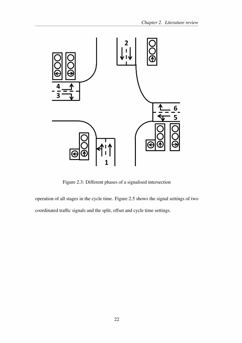
A traffic signal at an intersection could have red, amber and green lights to give
orders to road traffic. Following the order of the signal, traffic can make allowed
movements to pass the intersection. The term phase is used to refer to one or multi-
ple traffic movements which receive identical traffic signals at an intersection. Figure
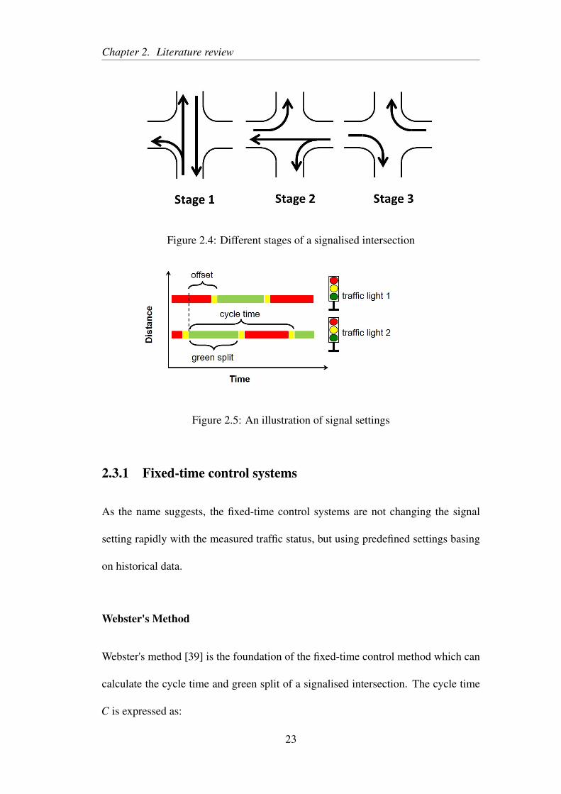
2.3 is an example where 6 different phases are set for the signalised intersection. The
term stage is defined as a compatible group of phases where they can process together
without having conflict. Figure 2.4 shows how the 6 phases are grouped into 3 stages.
There are three control variables which are generally used for the traffic signal set-
tings: split, offset and cycle time. The duration of a stage is equivalent to the green
light given to the traffic movements and known as split. Offset is the time difference
between adjacent signals for coordination. The total time required is for a complete
21
Chapter 2. Literature review
Figure 2.3: Different phases of a signalised intersection
operation of all stages in the cycle time. Figure 2.5 shows the signal settings of two
coordinated traffic signals and the split, offset and cycle time settings.
22
Chapter 2. Literature review
Figure 2.4: Different stages of a signalised intersection
Figure 2.5: An illustration of signal settings
2.3.1 Fixed-time control systems
As the name suggests, the fixed-time control systems are not changing the signal
setting rapidly with the measured traffic status, but using predefined settings basing
on historical data.
Webster's Method
Webster's method [39] is the foundation of the fixed-time control method which can
calculate the cycle time and green split of a signalised intersection. The cycle time
C is expressed as:
23
Chapter 2. Literature review
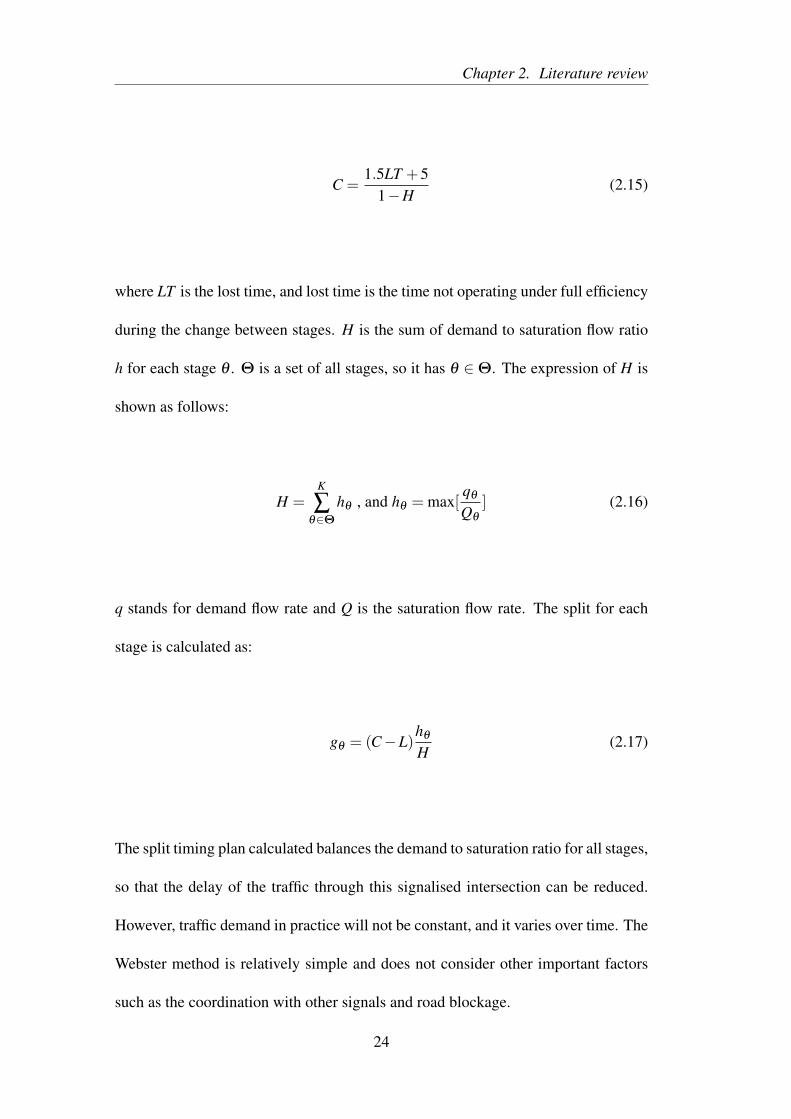
C =1.5LT +5
1−H(2.15)
where LT is the lost time, and lost time is the time not operating under full efficiency
during the change between stages. H is the sum of demand to saturation flow ratio
h for each stage θ . Θ is a set of all stages, so it has θ ∈Θ. The expression of H is
shown as follows:
H =K
∑θ∈Θ
hθ , and hθ = max[qθ
Qθ
] (2.16)
q stands for demand flow rate and Q is the saturation flow rate. The split for each
stage is calculated as:
gθ = (C−L)hθ
H(2.17)
The split timing plan calculated balances the demand to saturation ratio for all stages,
so that the delay of the traffic through this signalised intersection can be reduced.
However, traffic demand in practice will not be constant, and it varies over time. The
Webster method is relatively simple and does not consider other important factors
such as the coordination with other signals and road blockage.
24
Chapter 2. Literature review
TRANSYT - Traffic Network Study Tool
A centralised fixed-time system, which has been widely used in practice, is the Traf-
fic Network Study Tool (TRANSYT) [40, 41]. TRANSYT optimises the signal plans
for all traffic signals within the controlled area. It can estimate network performance
via a platoon dispersion model, and uses a hill climbing search algorithm to look
for the signal timing plans that give the best performance. The search algorithm
evaluates different split and offset values in order to bring an improvement to the
performance. The process of finding the signal plan is similar with other studies on
the fixed-timing system [42, 43] and can be summarised as the following optimisa-
tion problem:
minU
f (q,U) (2.18)
where q is the traffic flows in the network, and U is the signal timing plans which
include split, offset, cycle time for each intersection.
Fixed-time systems can achieve coordination in traffic signals and provide reason-
able plans for the controlled network. It modifies the plans for busy roads and peak
hours of a day. As fixed-time systems relying on historical data, the challenges come
from the unpredictable incidents and dynamic travel demands. Incidents like car ac-
cident and signal failure can lead to rapid changes in driving routes. Meanwhile, the
historical data has to be updated regularly. Bell and Bretherton [44] found the ageing
of fixed-time plans causes 3% per year in performance drop. Under the pressure of
25
Chapter 2. Literature review
the above issues, traffic-responsive control systems became more and more popular.
2.3.2 Traffic-responsive control systems
Traffic-responsive control systems process the collect flow data and derive efficient
signal plans to the traffic signals in the controlled network. Comparing to the fixed-
time control, it can response to traffic fluctuation and adjust plans actively. The
traffic-responsive control system generally requires a centralised control for coordi-
nation between traffic signals.
SCOOT - Split Cycle Offset Optimisation Technique
SCOOT (Split Cycle Offset Optimisation Technique) is a real-time centraliased con-
trol system, and the traffic information are collected from road detectors. SCOOT
has three key features: measuring cyclic flow profiles, updating queues continuously
for online control and use of incremental optimization for deriving signal plans.
Based on the traffic status across an urban network, the system continuously opti-
mises and updates the traffic signal plans to minimise stops and delays of vehicles.
Within the network controlled by SCOOT, signal plans for all signal controllers are
optimised together by a central computer. Therefore, SCOOT has a centralised con-
trol structure. While updating traffic signal plans, SCOOT can have a frequency of
10,000 times per hour for modifying 100 traffic signals within one network [45].
The advantage of using SCOOT is to adapt to the short-term changes of traffic. A
previous study showed that additional 12% of the delay can be reduced by SCOOT
compared to an up-to-date fixed time system [46].
26
Chapter 2. Literature review
SCATS - Sydney Coordinated Adaptive Traffic System
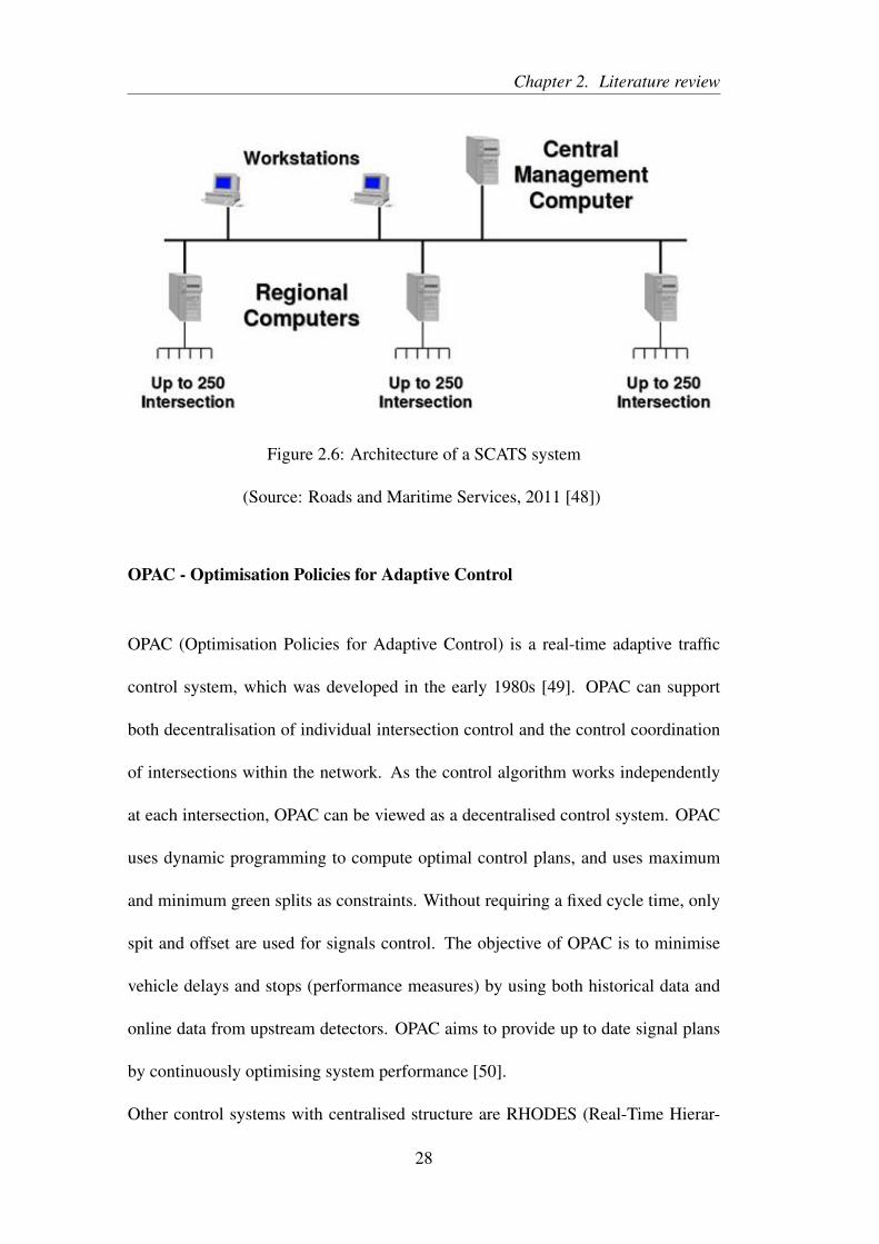
SCATS (Sydney Coordinated Adaptive Traffic System) is a centralised hierarchical
control system [47, 48], and generally consists of one central management computer,
regional computers and local controllers (see Figure 2.6). SCATS is a phase-based
control system, and uses cycle time, phase split and offset as control parameters.
Regional computers make strategic decisions at the upper control level which is to
determine all the control parameters based on its control area's traffic conditions.
The local controller makes tactical decisions at the lower control level, and it can
terminate the green light earlier or skip the entire phase when the locally measured
traffic demand is low. As local controllers control the signal settings, it can not
modify the control settings made from a higher control level. For example, when
it is necessary need to coordinate traffic signals for a main road, local controllers
can not omit the green phase on the main road. This is due to a common cycle time
needed for the coordination. The value range of signal timings that a local controller
can modify depends on the regional computer.
27
Chapter 2. Literature review
Figure 2.6: Architecture of a SCATS system
(Source: Roads and Maritime Services, 2011 [48])
OPAC - Optimisation Policies for Adaptive Control
OPAC (Optimisation Policies for Adaptive Control) is a real-time adaptive traffic
control system, which was developed in the early 1980s [49]. OPAC can support
both decentralisation of individual intersection control and the control coordination
of intersections within the network. As the control algorithm works independently
at each intersection, OPAC can be viewed as a decentralised control system. OPAC
uses dynamic programming to compute optimal control plans, and uses maximum
and minimum green splits as constraints. Without requiring a fixed cycle time, only
spit and offset are used for signals control. The objective of OPAC is to minimise
vehicle delays and stops (performance measures) by using both historical data and
online data from upstream detectors. OPAC aims to provide up to date signal plans
by continuously optimising system performance [50].
Other control systems with centralised structure are RHODES (Real-Time Hierar-
28
Chapter 2. Literature review
chical Optimized Distributed Effective System) [51, 52], TUC (Traffic-Responsive
Urban Control) [53, 54]. With a decentralised structure, the UTOPIA (Urban Traf-
fic Optimisation by Integrated Automation) [55, 56] system has been implemented
in several cities in Europe. Each of its signal controllers is integrated with a in-
dustrial computer named SPOT (System for Priority and Optimisation of Traffic).
This SPOT unit determines control parameters (cycle time, offset, split) accord-
ing to the detected local traffic volumes. SPOT units share the signal plans and
traffic data with adjacent ones. Public transport forecast, coordination criteria and
other control parameters are established by the central computer. Recently, re-
searches have paid great attention to developing the decentralised control systems
[57, 6, 58, 9, 59, 11, 60, 10]. Lammer and Helbing [59, 10] introduced a decen-
tralised self-organised control system with a stabilisation mechanism. Max-pressure
[6, 8, 61] (also known as BackPressure) is a decentralised control system which op-
erates through the upstream and downstream queuing at each intersections. A leader-
follower coordination framework [58] has been proposed to enhance the cooperation
between decentralised controllers.
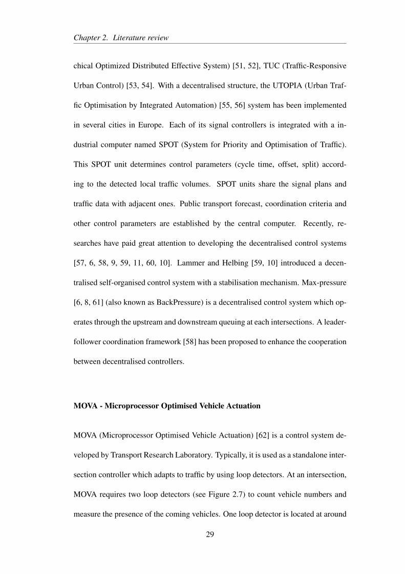
MOVA - Microprocessor Optimised Vehicle Actuation
MOVA (Microprocessor Optimised Vehicle Actuation) [62] is a control system de-
veloped by Transport Research Laboratory. Typically, it is used as a standalone inter-
section controller which adapts to traffic by using loop detectors. At an intersection,
MOVA requires two loop detectors (see Figure 2.7) to count vehicle numbers and
measure the presence of the coming vehicles. One loop detector is located at around
29

Chapter 2. Literature review
Figure 2.7: Locations of MOVA system's loop detectors
(Source: Crabtree, 2011 [62])
40m from the stopline which is referred to as ‘X-detector’. Another loop detector,
known as ‘IN-detector’, is located around 100m from the stopline. MOVA has two
operation modes, where it minimises the vehicle delay and stops in the undersatu-
rated condition and maximises the capacity in the oversaturated condition. In the
undersaturated condition, the decision on switch to the next stage or extend the cur-
rent stage is based on whether change can benefit the traffic on reducing delays and
stops. In the oversaturated condition, MOVA prioritises the oversaturated road by
extending its green light time, consequently, the signal is likely to operate with a
longer cycle time.
2.3.3 Discussion
This section has discussed the urban traffic control systems with different control
structures. The fixed-time system is first used to operate traffic signals in urban ar-
eas. It is an offline control and uses predefined signal plans which rely on historical
30
Chapter 2. Literature review
data. The common challenge of the fixed-time system is to handle unpredictable
disruptions and traffic fluctuations on a road network. Traffic-responsive systems
are introduced afterwards which is an online real-time control. Traffic-responsive
systems differ in control structure and can be classified into centralised and decen-
tralised control systems. Majority of the systems using in cities (e.g. SCOOT and
SCATS) have a centralised control structure where the signal plans are derived from
a central computer or regional computer and each of them can control more than a
hundred traffic signals. In contrast to the centralised control structure, the decen-
tralised systems are operated independently at each intersection. It is not common
to see a fully decentralised system operate on a urban network, and the decentralised
system may require a certain degree of centralised coordination.
In this study, the centralised and decentralised systems are going to be compared
in performance. A fully decentralised system is relatively new in the field and still
under development. Chapter 3 analyses the centralised and decentralised control
systems which will be used in the experiment, and explains the differences between
the two at the operational level. The next section focuses on optimisation technique,
which used to derive an optimal signal plan for a centralised traffic signal control
system.
31
Chapter 2. Literature review
2.4 Optimisation methods for signal control
In centralised traffic control systems, optimisation techniques are implemented to
derive traffic signal plans with associated traffic demands. There exist many optimi-
sation methods and choosing the right method needs to consider the control problem
feature, computational time and any other factors.
2.4.1 Formulation of the traffic signal control problem
In order to search for an optimal signal plan for a traffic signal control problem, it is
generally formulated in an optimisation problem format. An optimisation problem
consists three components: an objective function, constraints and decision variables.
The objective function usually minimises or maximises a system performance mea-
sure. The operational objective of a traffic control system is to improve traffic perfor-
mance on a road network. Various performance measures have been used to evaluate
the traffic signal settings of a traffic control system, such as delay and queue length.
Delay is the number of vehicle-hour where traffic waited during the red light signal.
Queue length is another performance measure where it is the number of vehicles
cannot be clear by the end of a green signal. Other performance measures such as
phase utilisation and green bandwidth also reflect the performance of signal settings
at the signalised intersections. The constraints of an optimisation problem define
the range of feasible solutions. The constraints for a signal control problem can be
traffic dynamics and traffic signal settings. Traffic dynamics’ constraints describe
how traffic could propagate in a road network. For example, a road could have a 30
32
Chapter 2. Literature review
mph speed limit and the capacity of the road could be 230 vehicles per mile. Both
of the road properties can be defined in the optimisation problem by constraints. In
terms of the traffic signal settings, a signal controller could have a cycle time which
equals to 100 seconds. In this case, the traffic signal plan should repeat every 100
seconds. This need to be defined in the optimisation problem by constraints as well.
Decision variables form the solution of an optimisation problem. When the optimi-
sation problem minimises the network delay through traffic signal plans, the signal
plans are the decision variables. Both of the objective function and constraints are
functions of the decision variables.
Delay is one of the most popular performance measure used as the objective func-
tion for a traffic signal control problem. It describes the loss of efficiency in the
traffic control system under both undersaturated and oversaturated cases. Delay is
calculated as the difference between actual vehicle hour travelled (VHT) and vehicle
distance travelled (VDT) under free flow speed υf. The VHT is the number of vehi-
cles on a link i at a time step t:
V HTi(t) = ρi(t)llink∆t (2.19)
where ρ is the traffic density on the link i, l is the length of the road link and ∆t is
the interval of a time step. The VDT is the number of vehicle flow through the link i
and formulated as:
33
Chapter 2. Literature review
V DTi(t) = qi(t)llink∆t (2.20)
The expression of the delay on a link i at a time step t is:
T ND(t) =I
∑i=1
V HTi(t)−V DTi(t)/υf (2.21)
The traffic flow model CTM could be converted into constraints of an optimisation
problem. It is a macroscopic flow model and capsules flow dynamics such as for-
mation and dissipation of traffic queues (see Section 2.2.2). CTM splits a road into
sections (cells), and the traffic density of a cell c at time step t is defined as follow:
ρc(t +1) = ρc(t)+∆t
lcellc
[qc−1(t)−qc(t)] (2.22)
where the traffic flow q of cell c at time t is:
qc(t) = min{
υcρc(t),Qc,Qc+1,wc+1[ρjam,c+1−ρc+1(t)
]}(2.23)
In order to convert the traffic dynamics of CTM into an optimisation problem, the
nonlinear equation 2.23 are modified into four linear inequality constraints [63] [64]:
34
Chapter 2. Literature review
qc(t)≤ υcρc(t)
qc(t)≤ Qc
qc(t)≤ Qc+1
qc(t)≤ wc+1[ρjam,c+1−ρc+1(t)
](2.24)
The traffic signal plans are the decision variables for a traffic signal control prob-
lems. When operating traffic signals, time unit usually is second which means all the
decision variables are positive integers. In this case, additional integer constraints
are added to the traffic signal control problem and it is known as a mixed-integer
optimisation problem. In Lo’s study [63], the network signal control problem is for-
mulated as a mixed-integer programming model with the traffic flow model CTM
(see Section 2.2.2). The traffic signals are simulated by the binary variables at the
last cells of incoming links to a signalised intersection. Assuming the traffic signal
has two stages, θ(t) = 1 for stage one and θ(t) = 0 for stage two. The maximum
flow rate of the last cells of two incoming links c1 and c2 at an intersection can be
formulated as follows:
Qc1(t) = θ(t)Qc1
Qc2(t) = [1−θ(t)]Qc2
θ(t) ∈ [0,1]
(2.25)
When the stage index θ = 1, the maximum flow rate for stage 2 traffic will be zero
35
Chapter 2. Literature review
and verse vice. Another variable ι is used to indicate the change of stages [66] and
have:
ι(t) = |θ(t)−θ(t−1)| (2.26)
where the equation is equivalent to inequality equations as follows:
θ(t)−θ(t−1)≤ ι(t)≤ θ(t)+θ(t−1)
−θ(t)+θ(t−1)≤ ι(t)≤ 2−θ(t)−θ(t−1)
(2.27)
When there is a change of stage at time step t, ι(t) = 1. A signal plan with green
split g can be formulated as:
g(k) =kC
∑(k−1)C+1
θ(t) (2.28)
The green split needs to be in its feasible range, so that it has the constraint:
gmin ≤ g≤ gmax (2.29)
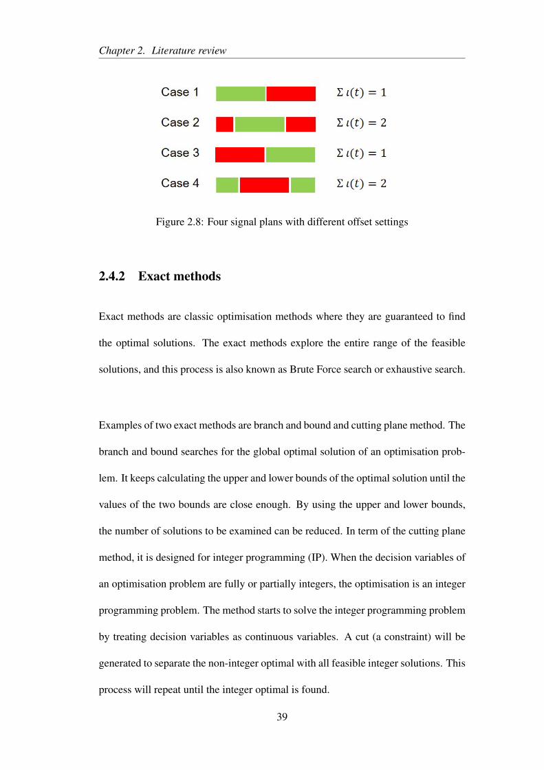
In terms of the offset o, it can started at anytime from the first time step to the last
one within a signal cycle. Since the traffic signal is assumed only have two stages,
the offset o is always the start time step of stage 1. When t = o, it will have θ(t) = 1
and ι(t) = 1. With offset control, there are four cases for a cycle signal plan (see Fig-
36
Chapter 2. Literature review
ure 2.8), the following constraint is held to capture the signal plan with offset control:
0≤kC
∑(k−1)C+1
ι(t)−1≤ 1 where ι(t) ∈ [1,2] (2.30)
The final formulation of the traffic signal control problem is:
mint=T
∑t=1
∑c∈C
(ρc(t)−qc(t)/υf)lcell∆t
subject to
ρc(t +1) = ρc(t)+∆t
lcellc
[qc−1(t)−qc(t)]
Qclastj,1(t) = θ j(t)Qclast
j,1
Qclastj,2(t) = [1−θ j(t)]Qclast
j,2
g j,1(k) =kC
∑(k−1)C+1
θ j(t)
qc(t)≤ υcρc(t)
qc(t)≤ Qc
qc(t)≤ Qc+1
qc(t)≤ wc+1[ρjam,c+1−ρc+1(t)
]
37
Chapter 2. Literature review
θ j(t)−θ j(t−1)≤ ι j(t)≤ θ j(t)+θ j(t−1)
−θ j(t)+θ j(t−1)≤ ι j(t)≤ 2−θ j(t)−θ j(t−1)
gmin ≤ g j,1 ≤ gmax
0≤kC
∑(k−1)C+1
ι j(t)−1≤ 1
θ j(t) ∈ [0,1]
ι j(t) ∈ [1,2]
Apart from the mixed integer optimisation problem, there are other examples where
a traffic signal control problem is formulated in the continuous model instead of a
discrete one. TUC system [54] uses a Store-and-Forward model which models the
signal controlled traffic as a continuous flow and a time step equals to a signal cycle
time. The flow model does simplify the formulation of the signal control problem
and avoided the integer constraints. However, it is not an accurate description traffic
queues formed by traffic signal [65].
Since the traffic signal control problem is formulated in the optimisation format, the
following two sections (Section 2.4.2 and Section 2.4.3) present groups of searching
methods which can solve this optimisation problem.
38
Chapter 2. Literature review
Figure 2.8: Four signal plans with different offset settings
2.4.2 Exact methods
Exact methods are classic optimisation methods where they are guaranteed to find
the optimal solutions. The exact methods explore the entire range of the feasible
solutions, and this process is also known as Brute Force search or exhaustive search.
Examples of two exact methods are branch and bound and cutting plane method. The
branch and bound searches for the global optimal solution of an optimisation prob-
lem. It keeps calculating the upper and lower bounds of the optimal solution until the
values of the two bounds are close enough. By using the upper and lower bounds,
the number of solutions to be examined can be reduced. In term of the cutting plane
method, it is designed for integer programming (IP). When the decision variables of
an optimisation problem are fully or partially integers, the optimisation is an integer
programming problem. The method starts to solve the integer programming problem
by treating decision variables as continuous variables. A cut (a constraint) will be
generated to separate the non-integer optimal with all feasible integer solutions. This
process will repeat until the integer optimal is found.
39
Chapter 2. Literature review
The advantages of the exact methods come from their simplicity for implementa-
tion and its accuracy in solution. However, the simplicity and the accuracy lead the
searching process to be time-consuming and resource intensive. An exact method is
suitable when the optimisation problem has a smaller number of feasible solutions. It
is not popular in real-world problems which are complex and has large dimensions.
This is also a reason why it has not been widely implemented for traffic signal oper-
ations. Gartner [67] [68] has formulated a traffic signal (offset) control problem in
an mixed-integer linear programming model. The objective function is to maximise
the bandwidth (green wave) between coordinated traffic signals. Both exact method
and heuristic method are used where the heuristic is around 100-300 times faster in
running time without significantly compromising the quality of its solution.
2.4.3 Heuristic methods
In contrast with the exact methods, heuristic methods are used to solve a complex
problem within a limited time. The heuristic methods do not search for the global
optimal but near-optimal solutions. The heuristic methods sacrifice the quality of
the solution to save the running time, and they have less restrictions when mod-
elling a optimisation problem. Some examples of the popular heuristic methods used
to solve traffic control problems are Genetic Algorithm, Ant Colony Optimisation,
Tabu Search and Simulated Annealing.
40
Chapter 2. Literature review
Genetic Algorithm
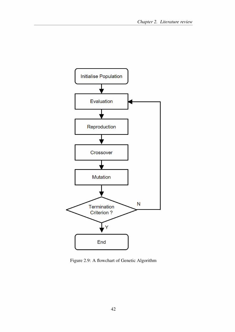
Genetic Algorithm (GA) [69] is a heuristic search, which mimics the natural selec-
tion process. It uses existing ‘good’ solutions to regenerate new solutions iteratively
until a near optimal solution is achieved. GA is a population-based approach, where
a group of solutions are evaluated all together for each time of regeneration. The
regeneration process includes: reproduction, crossover and mutation. They ensure
the characters of the better solutions can be passed on to the next generation of so-
lutions. The regeneration process will run iteratively until meeting the termination
criterion (e.g. maximum number of iterations or only limited improvement can be
made in solutions). A flowchart of GA is shown in Figure 2.9. Lo and Chow [70]
implemented GA to derive signal timing plans which minimised the total delay of an
urban arterial network. BALANCE [71] is an existing traffic control system using
GA to optimise signal plans. It operates in Hamburg, Ingolstadt and other cities in
Germany.
41
Chapter 2. Literature review
Figure 2.9: A flowchart of Genetic Algorithm
42
Chapter 2. Literature review
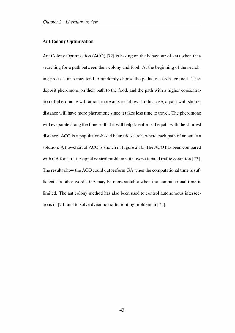
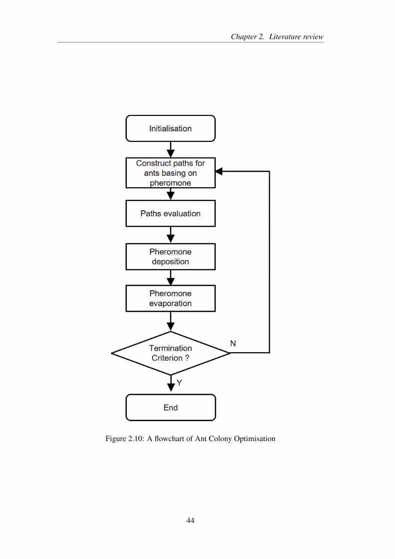
Ant Colony Optimisation
Ant Colony Optimisation (ACO) [72] is basing on the behaviour of ants when they
searching for a path between their colony and food. At the beginning of the search-
ing process, ants may tend to randomly choose the paths to search for food. They
deposit pheromone on their path to the food, and the path with a higher concentra-
tion of pheromone will attract more ants to follow. In this case, a path with shorter
distance will have more pheromone since it takes less time to travel. The pheromone
will evaporate along the time so that it will help to enforce the path with the shortest
distance. ACO is a population-based heuristic search, where each path of an ant is a
solution. A flowchart of ACO is shown in Figure 2.10. The ACO has been compared
with GA for a traffic signal control problem with oversaturated traffic condition [73].
The results show the ACO could outperform GA when the computational time is suf-
ficient. In other words, GA may be more suitable when the computational time is
limited. The ant colony method has also been used to control autonomous intersec-
tions in [74] and to solve dynamic traffic routing problem in [75].
43
Chapter 2. Literature review
Figure 2.10: A flowchart of Ant Colony Optimisation
44
Chapter 2. Literature review
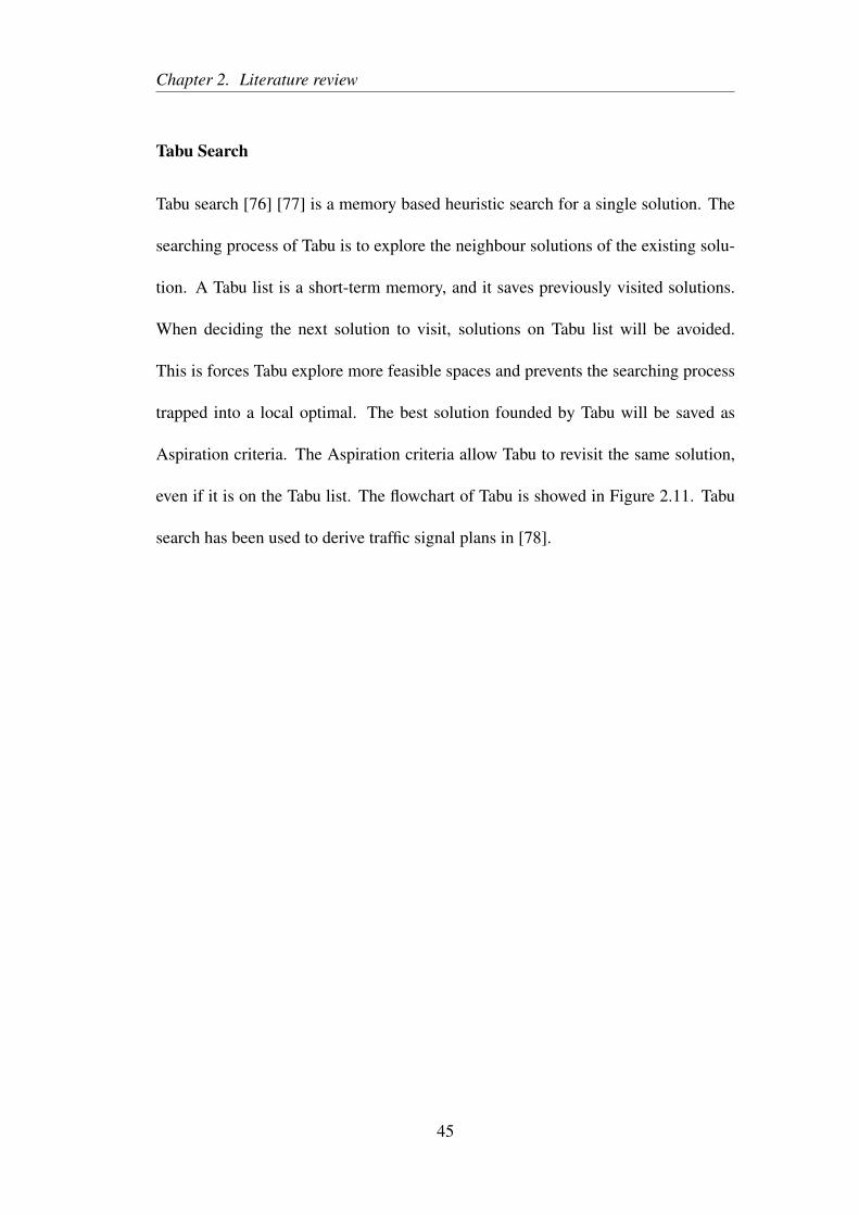
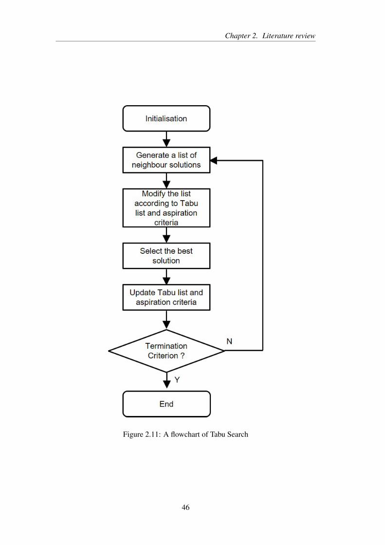
Tabu Search
Tabu search [76] [77] is a memory based heuristic search for a single solution. The
searching process of Tabu is to explore the neighbour solutions of the existing solu-
tion. A Tabu list is a short-term memory, and it saves previously visited solutions.
When deciding the next solution to visit, solutions on Tabu list will be avoided.
This is forces Tabu explore more feasible spaces and prevents the searching process
trapped into a local optimal. The best solution founded by Tabu will be saved as
Aspiration criteria. The Aspiration criteria allow Tabu to revisit the same solution,
even if it is on the Tabu list. The flowchart of Tabu is showed in Figure 2.11. Tabu
search has been used to derive traffic signal plans in [78].
45
Chapter 2. Literature review
Figure 2.11: A flowchart of Tabu Search
46
Chapter 2. Literature review
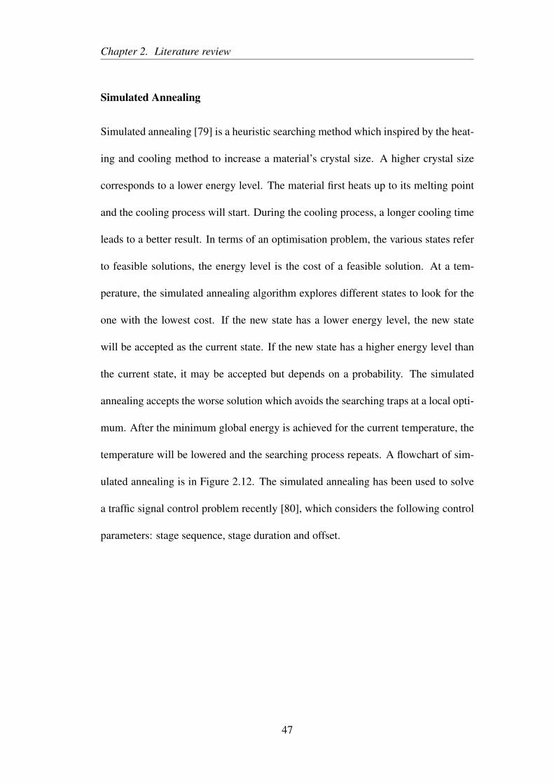
Simulated Annealing
Simulated annealing [79] is a heuristic searching method which inspired by the heat-
ing and cooling method to increase a material’s crystal size. A higher crystal size
corresponds to a lower energy level. The material first heats up to its melting point
and the cooling process will start. During the cooling process, a longer cooling time
leads to a better result. In terms of an optimisation problem, the various states refer
to feasible solutions, the energy level is the cost of a feasible solution. At a tem-
perature, the simulated annealing algorithm explores different states to look for the
one with the lowest cost. If the new state has a lower energy level, the new state
will be accepted as the current state. If the new state has a higher energy level than
the current state, it may be accepted but depends on a probability. The simulated
annealing accepts the worse solution which avoids the searching traps at a local opti-
mum. After the minimum global energy is achieved for the current temperature, the
temperature will be lowered and the searching process repeats. A flowchart of sim-
ulated annealing is in Figure 2.12. The simulated annealing has been used to solve
a traffic signal control problem recently [80], which considers the following control
parameters: stage sequence, stage duration and offset.
47
Chapter 2. Literature review
Figure 2.12: A flowchart of Simulated Annealing
48
Chapter 2. Literature review
2.4.4 Discussion
The Section 2.4.2 and Section 2.4.3 explain various optimisation algorithms which
used in centralised traffic control systems for deriving optimal signal plans. The ex-
act method and heuristic method are two main types of the algorithms. An exact
method looks for a global optimal solution and explores all feasible solutions. How-
ever, it generally requires long computational time and difficult to implement in real
life problems. A heuristic method looks for local optimal solutions. It requires less
execution time and can be applied to a wider range of optimisation problems. The
heuristic method is more practical to use when the time is limited and global optimal
solution is not necessary.
In this study, both of the exact method and heuristic method are going to be used
which derive global optimal and local optimal solutions. A brute force approach is
a simulation-based exact method. It is easy to implement and guarantees to find the
best solution. It is not a practical method but gives a benchmark to compare the
centralised control solution with other decentralised ones. In terms of the heuris-
tic method, several modern techniques have been reviewed and all have been used
to solve traffic signal control problems (see Section 2.4.3). Table 2.1 summarises
the characteristics of all the heuristic method mentioned in the previous section and
it is based on the classification in [81]. The first criterion in the table is the use
of memory. The memoryless method indicates that the use of memory in heuristic
methods do not have an impact on the searching process. Heuristic methods like
Tabu search require memory from the computer to record a list of solutions where
49
Chapter 2. Literature review
they have visited. The list will keep growing during the searching process, since the
Tabu list tracks the solutions with bad performance or visited solutions. This is also
the reason why Tabu search is not considered to use in this study. The next criterion
on the table is neighbourhood exploration type. The trajectory method chooses adja-
cent solutions where the discontinuous method chooses any locations in the feasible
range. Comparing to the trajectory method, the discontinuous method involves more
randomness and could explore the full range of the feasible solutions faster. Follow-
ing the neighbourhood exploration, the heuristic methods are different in the types of
their solutions. As the name suggests, the population-based solution means a search-
ing method handles a group of solutions at the same time. The single point search
visits only one solution each time. The simulated annealing method uses single point
search. Due to the size of a traffic signal control problem, simulated annealing may
be too slow to explore a large solution space. Therefore, simulated annealing is not
in use for this study as well. Modern computers all have multi-core processors which
can carry out multiple calculation tasks at the same time. This kind of computation
is known as parallel computing. For example, an eight-core computer comparing
to a single-core computer, it can reduce the computational time from T to T/8 by
parallel computing. GA evaluates the performance of all solutions in a population
before generating a new population. The evaluation can be performed at the same
time by parallel computing, as the solutions are independent of each other. ACO
creates paths of ants basing on pheromone level. This process can also use paral-
leling computing to calculate the paths simultaneously. The last column in the table
explains the inspiration of each heuristic method. Comparing GA and ACO, they
50
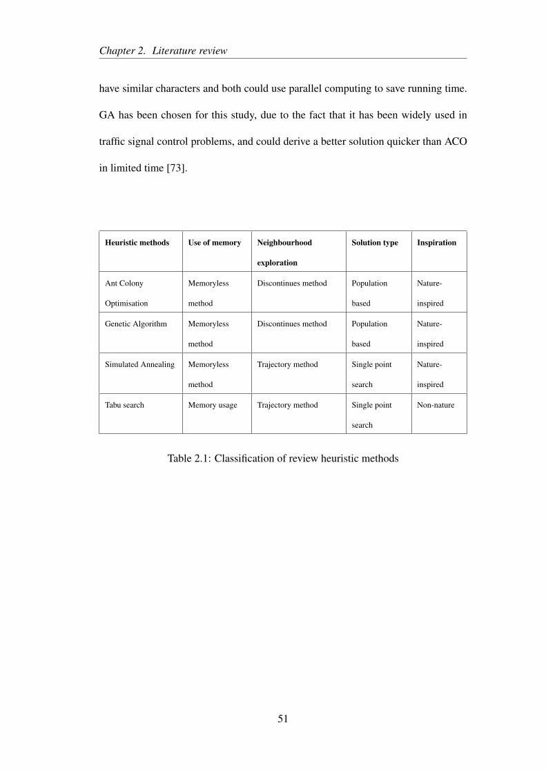
Chapter 2. Literature review
have similar characters and both could use parallel computing to save running time.
GA has been chosen for this study, due to the fact that it has been widely used in
traffic signal control problems, and could derive a better solution quicker than ACO
in limited time [73].
Heuristic methods Use of memory Neighbourhood
exploration
Solution type Inspiration
Ant Colony
Optimisation
Memoryless
method
Discontinues method Population
based
Nature-
inspired
Genetic Algorithm Memoryless
method
Discontinues method Population
based
Nature-
inspired
Simulated Annealing Memoryless
method
Trajectory method Single point
search
Nature-
inspired
Tabu search Memory usage Trajectory method Single point
search
Non-nature
Table 2.1: Classification of review heuristic methods
51
Chapter 3
Analysis of urban traffic control sys-
tems
3.1 Introduction
This chapter analyses the urban traffic control systems to be investigated in this study
in the following sections. Section 3.2 starts with two distinctive centralised control
systems, the brute force approach and the genetic algorithm. Section 3.3 presents two
semi-decentralised control systems: Traffic-responsive Urban Control (TUC) system
and its variant a Hybrid system. They are classified as semi-decentralised systems,
because two of the split and cycle time controls are optimised in a centralised way
and the offset control is decentralised. In Section 3.4, max-pressure is introduced
as a fully decentralised control system. At the end, Section 3.5 is a summary of the
chapter.
52
Chapter 3. Analysis of urban traffic control systems
3.2 Centralised control
3.2.1 Brute Force Approach
In a centralised system, all traffic information is sent to a central controller or agent
that is responsible for deriving and implementing all control actions. To derive an
optimal signal plan for such centralised systems, a straightforward way is by a ‘brute
force’ approach (BF) which calculates the performances of all feasible signal plans
and picks the signal plan that gives the best performance. Despite its ability to iden-
tify the true global optimal solution, this brute force approach could take an enor-
mous computational time and the amount of computation grows exponentially as the
network size and number of decision variables increase [82]. The brute force ap-
proach therefore is rarely used in general applications. In this study, the Brute force
is implemented on Matlab 2013b, and used parallel computing tool ‘parfor’ to run-
ning evaluation of multiple solutions at the same time.
The brute force approach searches for optimal values of a signal plan. A signal plan
consists of three control parameters: cycle time, offset and green split. The time step
duration ∆t of the traffic flow model to be used is 1 second, so that all the control
parameters will be integers. The cycle time and offset are bounded by their feasible
ranges. There are two stages in one signal cycle, where the green splits for each
stage need to satisfy a lower bound and a cycle time constraint:
53
Chapter 3. Analysis of urban traffic control systems
gmin ≤ g1,g2
g1 +g2 =C−LT
(3.1)
where the g1 and g2 stand for the green splits of the two stages. The sum of the green
splits always equals to the cycle time C (excluding the lost time LT ). An illustration
of the feasible green splits is shown in Figure 3.1. The feasible green splits are the
integers located along the cycle time constraint and bounded by a minimum green
split value. Figure 3.2 demonstrates a signal plan used for the brute force approach.
A common cycle time C is used for all controllers, and each controller has a green
split g and an offset o for every cycle. The g1,1 stands for the green split for stage 1,
and the corresponding green split for stage 2 can be calculated from C−LT −g1,1.
It can be seen that the number of possible signal plans increase dramatically with the
controlled network size (number of controllers) and controlling period (number of
cycles).
54
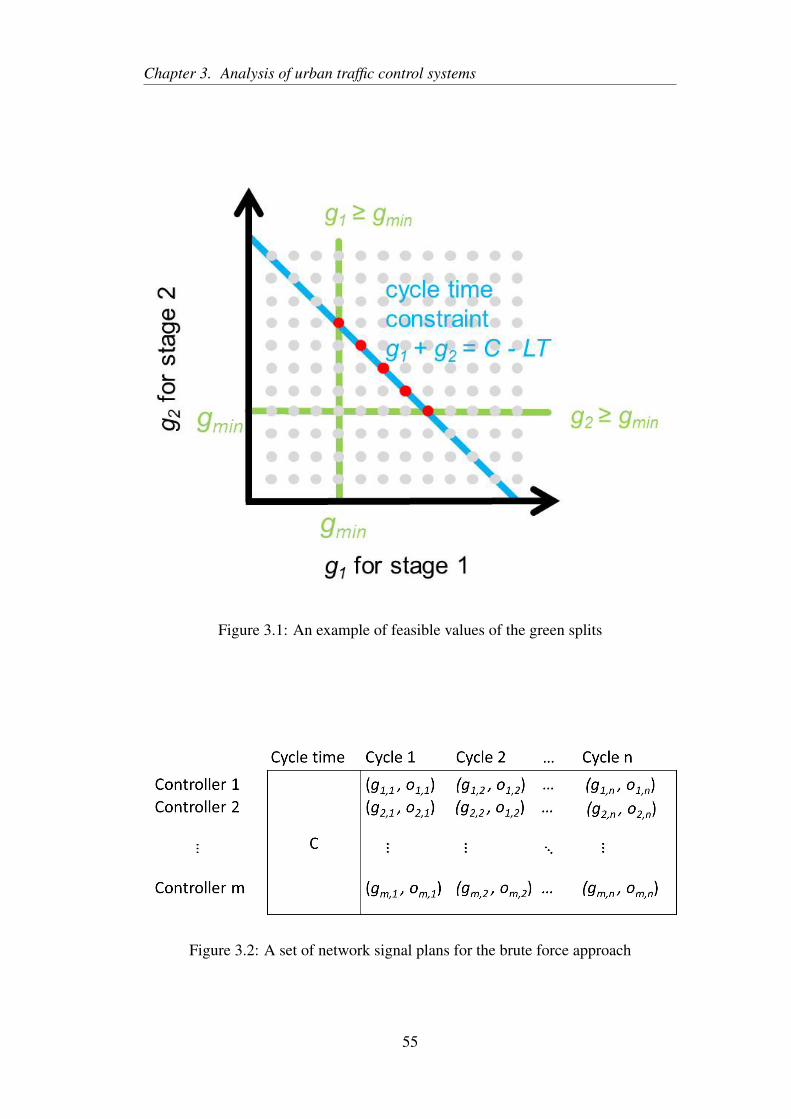
Chapter 3. Analysis of urban traffic control systems
Figure 3.1: An example of feasible values of the green splits
Figure 3.2: A set of network signal plans for the brute force approach
55
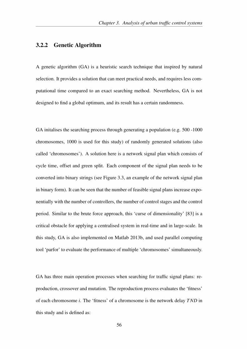
Chapter 3. Analysis of urban traffic control systems
3.2.2 Genetic Algorithm
A genetic algorithm (GA) is a heuristic search technique that inspired by natural
selection. It provides a solution that can meet practical needs, and requires less com-
putational time compared to an exact searching method. Nevertheless, GA is not
designed to find a global optimum, and its result has a certain randomness.
GA initalises the searching process through generating a population (e.g. 500 -1000
chromosomes, 1000 is used for this study) of randomly generated solutions (also
called ‘chromosomes’). A solution here is a network signal plan which consists of
cycle time, offset and green split. Each component of the signal plan needs to be
converted into binary strings (see Figure 3.3, an example of the network signal plan
in binary form). It can be seen that the number of feasible signal plans increase expo-
nentially with the number of controllers, the number of control stages and the control
period. Similar to the brute force approach, this ‘curse of dimensionality’ [83] is a
critical obstacle for applying a centralised system in real-time and in large-scale. In
this study, GA is also implemented on Matlab 2013b, and used parallel computing
tool ‘parfor’ to evaluate the performance of multiple ‘chromosomes’ simultaneously.
GA has three main operation processes when searching for traffic signal plans: re-
production, crossover and mutation. The reproduction process evaluates the ‘fitness’
of each chromosome i. The ‘fitness’ of a chromosome is the network delay T ND in
this study and is defined as:
56
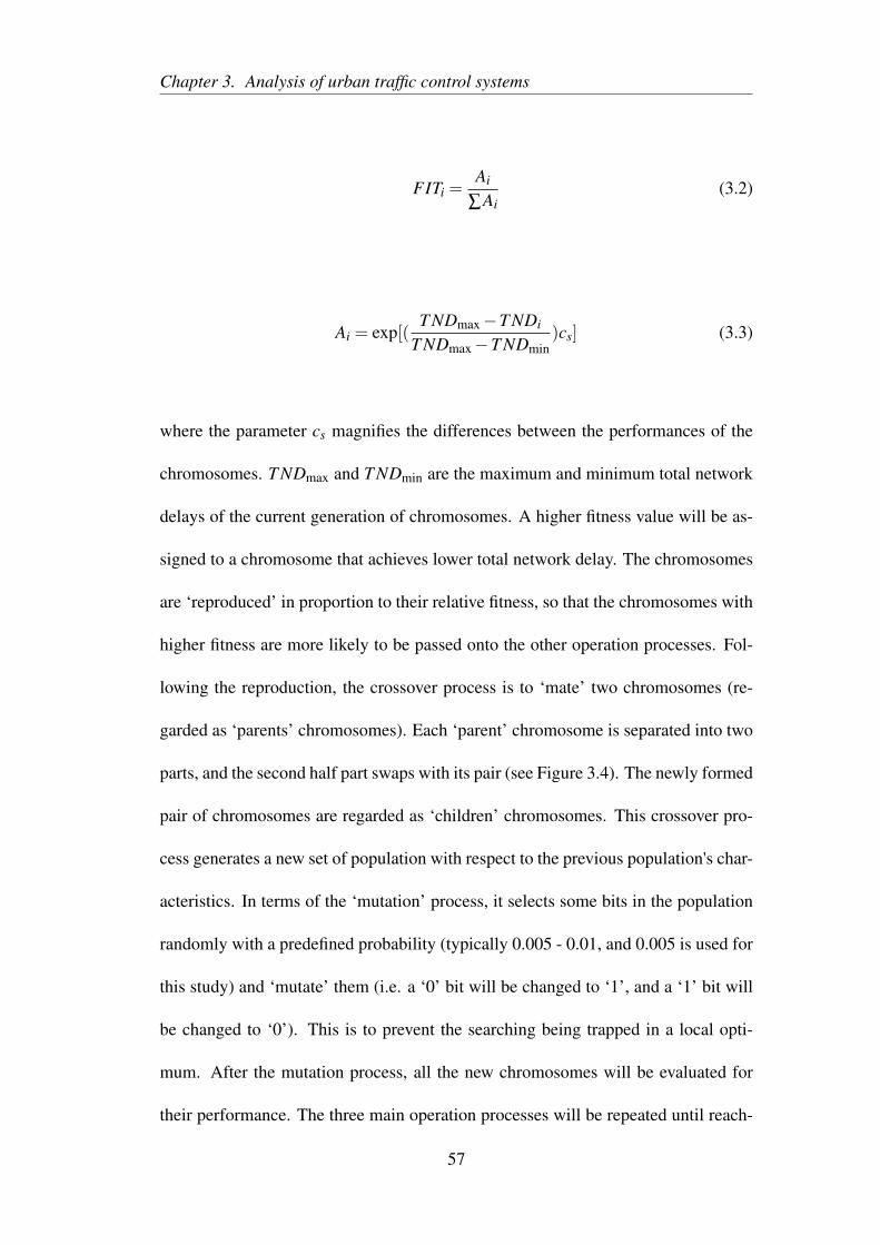
Chapter 3. Analysis of urban traffic control systems
FITi =Ai
∑Ai(3.2)
Ai = exp[(T NDmax−T NDi
T NDmax−T NDmin)cs] (3.3)
where the parameter cs magnifies the differences between the performances of the
chromosomes. T NDmax and T NDmin are the maximum and minimum total network
delays of the current generation of chromosomes. A higher fitness value will be as-
signed to a chromosome that achieves lower total network delay. The chromosomes
are ‘reproduced’ in proportion to their relative fitness, so that the chromosomes with
higher fitness are more likely to be passed onto the other operation processes. Fol-
lowing the reproduction, the crossover process is to ‘mate’ two chromosomes (re-
garded as ‘parents’ chromosomes). Each ‘parent’ chromosome is separated into two
parts, and the second half part swaps with its pair (see Figure 3.4). The newly formed
pair of chromosomes are regarded as ‘children’ chromosomes. This crossover pro-
cess generates a new set of population with respect to the previous population's char-
acteristics. In terms of the ‘mutation’ process, it selects some bits in the population
randomly with a predefined probability (typically 0.005 - 0.01, and 0.005 is used for
this study) and ‘mutate’ them (i.e. a ‘0’ bit will be changed to ‘1’, and a ‘1’ bit will
be changed to ‘0’). This is to prevent the searching being trapped in a local opti-
mum. After the mutation process, all the new chromosomes will be evaluated for
their performance. The three main operation processes will be repeated until reach-
57
Chapter 3. Analysis of urban traffic control systems
Figure 3.3: A chromosome structure of a network signal plan
ing a predefined maximum iteration (e.g. 20 to 30, 30 is used for this study).
In practice, GA needs to take different kinds of engineering constraints into con-
sideration. Decoding is a process here to convert the GA solutions (chromosomes)
into feasible signal plans. For example, when the maximum cycle time Cmax is set
equal to be 120 seconds, the offset can have a range from 0 to 120 seconds. The
corresponding binary string needs be sufficient to represent all of the possible values
for the feasible cycle time, offset and green split. A binary string with seven bits can
create 27 = 128 different integers from 0 to 127 to cover the possible values. A value
CI from a cycle time binary string can be ‘decoded’ as:
C = (CI127
)(Cmax−Cmin)+Cmin (3.4)
where Cmax and Cmin are the maximum and minimum values for feasible cycle time.
58
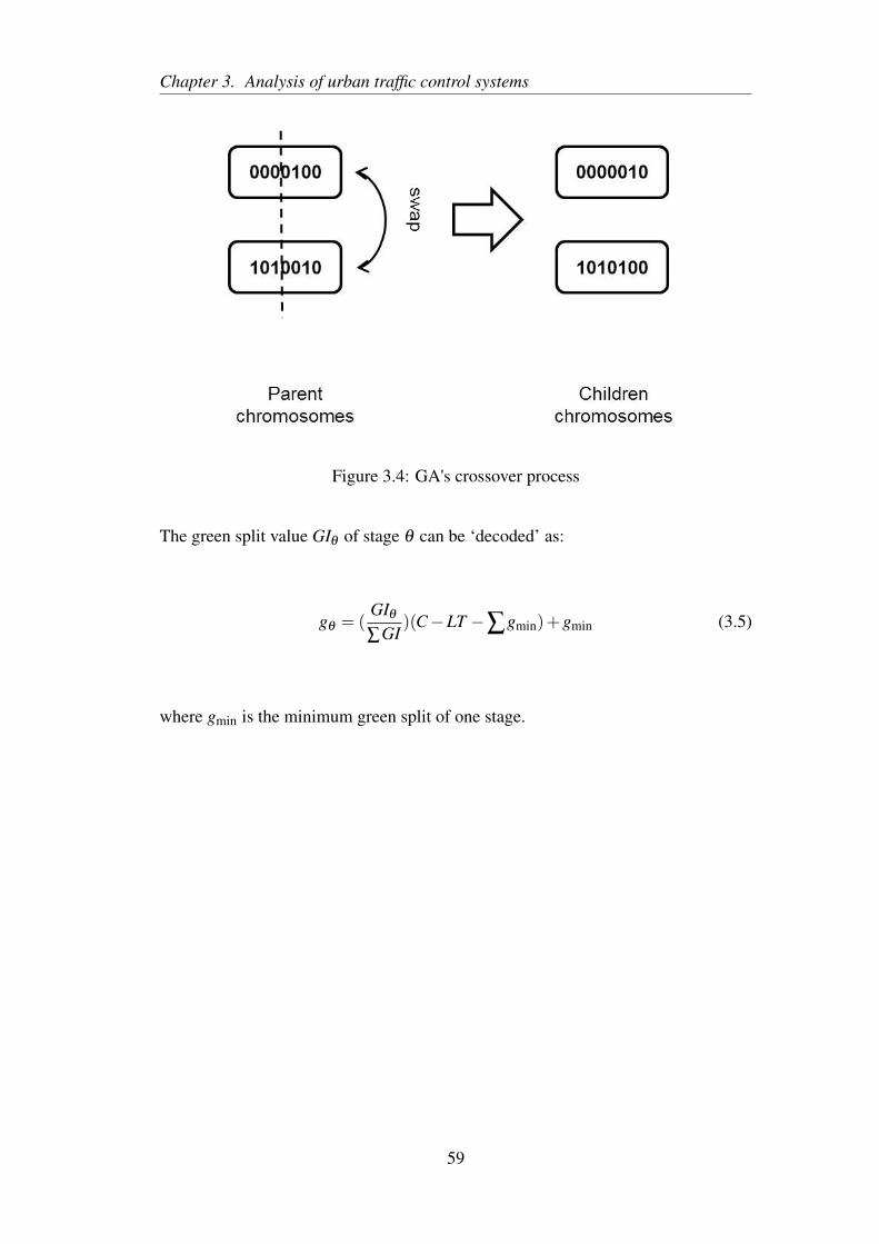
Chapter 3. Analysis of urban traffic control systems
Figure 3.4: GA's crossover process
The green split value GIθ of stage θ can be ‘decoded’ as:
gθ = (GIθ
∑GI)(C−LT −∑gmin)+gmin (3.5)
where gmin is the minimum green split of one stage.
59
Chapter 3. Analysis of urban traffic control systems
3.3 Semi-decentralised control
3.3.1 TUC system
The ‘semi-decentralised’ system is represented by a TUC [54] system and a hybrid
system (a variant of the TUC system). TUC system uses three control parameters:
green splits, offsets, and cycle time. The TUC is considered as a ‘semi-decentralised’
system in this study, since the cycle time is optimised in a centralised way, while the
green splits and offset controllers are decentralised.
Split Control
TUC adjusts green splits to minimise network queues. The green splits g = [gi] for
each road i is calculated from a centralised linear quadratic regulator (LQR) [54].
The LQR uses a store-and-forward model with a time interval ∆t set to be the cycle
time C. The LQR optimal control problem is formulated as:
min∆g(k)
Zn =12
∞
∑k=0
(x(k)T Sx(k)+∆g(k)T R∆g(k))
subject to x(k+1) = x(k)+B∆g(k) (3.6)
where x(k) is a vector of residual queue lengths x(k) = [xi(k)] for each road i by
the end of green light of cycle k. ∆g(k) is a vector of change in green splits. Reg-
ulating the ∆g(k) instead of g(k) in Equation 3.6 can avoid over fluctuation in the
green splits. ∆gi(k) = gi(k)− gNi where gN
i is the associated nominal green split.
60
Chapter 3. Analysis of urban traffic control systems
The S and R are both diagonal weighting matrices and they determine the trade-off
between minimising queues and adjusting the signal plan[54]. The diagonal ele-
ments of S(y,z)(y = z = i) are the reciprocals of road capacity 1xi,max
for road i, and
S(y,z) = 0 otherwise. R = rI where I is a identity matrix. The choice of r in R never-
theless will be a trial-and-error process so as to achieve the most satisfactory control
performance. It is noted that the original green split regulator is a centralised optimi-
sation model as it considers all roads i in (3.6) while recently there have been studies
(e.g. [11]) aiming to decompose (3.6) and hence operate it in a decentralised manner.
The optimality condition of (3.6) can be derived in the form of the following feed-
back control law [53] on green split g(k) allocated to each road i over each cycle k as:
g(k) = gN−Lx(k) (3.7)
where L is the corresponding control gain associated with each road i. The control
gain L, which will be dependent on S, R, and B where B is a diagonal matrix of ‘mi-
nus’ saturation flows in which B(y,z) =−Qi if y = z = i, and B(y,z) = 0 otherwise.
To determine L, the matrix can be derived from the Hamilton-Jacobi-Bellman (HJB)
equation. Suppose that Z∗(xk) is the optimal ‘cost-to-go’ function at cycle k with
state xk, the HJB equation can be written as:
Z∗(xk) = min∆g(k)
[(xTk Sxk +∆gT
k R∆gk)+Z∗(xk+1)]
= min∆g(k)
[(xTk Sxk +∆gT
k R∆gk)+Z∗(xk +B∆gk)]
(3.8)
61
Chapter 3. Analysis of urban traffic control systems
It is known that the optimal cost-to-go function Z∗ is quadratic in x, i.e. Z∗(xk) =
xTk Pxk, for some matrix P = PT ≥ 0 and all k. Hence, the HJB equation can be
rewritten as:
xTk Pxk = min
∆g(k)[(xT
k Sxk +∆gTk R∆gk)+(xk +S∆gk)
T P(xk +S∆gk)] (3.9)
Differentiating the right-hand side with respect to ∆gk gives the corresponding deriva-
tive: 2R∆gk +2BP(xk +B∆gk). Setting this derivative to zero, the optimal ∆gk can
be obtained as:
2R∆gk +2BT P(xk +B∆gk) = 0
⇒ ∆gk =−(R+BT PB)−1BT Pxk
⇒ ∆gk = Lxk
(3.10)
The matrix L expressed as:
L =−(R+BT PB)−1BT P (3.11)
By substitute ∆gk, ∆gk = gk−gN , into the (3.9), it gives:
xTk Pxk = (xT
k Sxk +∆gTk R∆gk)+(xk +B∆gk)
T P(xk +B∆gk)
= xTk (S+P−PB(R+BT PB)−1BT P)xk
(3.12)
62
Chapter 3. Analysis of urban traffic control systems
According to (3.12), the matrix P in (3.11) can be determined by solving the follow-
ing Riccati equation:
P = S+P−PB(R+BT PB)−1BT P (3.13)
Equation 3.13 can be solved readily by various numerical solution packages , such
as the ‘dlqr’ package in MATLAB. An example of how to derive the control gain
L matrix is in Appendix B. By considering an infinite horizon in time k in (3.6),
the control gain L can be calculated offline as the steady-state solution to (3.11).
Consequently, the control law (3.7) can be operated readily with feeding informa-
tion of queue lengths x in real-time without solving any optimisation problem. This
makes TUC a more computationally effective system than other centralised algo-
rithms such as GA for real-time operations. Previous studies show that the setting of
nominal green gN would play an important role in defining the performance of the
TUC. To address this, [54] presents a revised TUC control rule:
g(k) = g(k−1)−L[x(k)−x(k−1)] (3.14)
by subtracting (3.7) for cycle (k− 1) from (3.7) for cycle k. The advantage of us-
ing (3.14) over (3.7) is that it does not require predefining the nominal green gN . As
shown, the crucial information for operating TUC is the observation of queue lengths
x. In the CTM, this can be estimated by determining the number of cells (or length
63
Chapter 3. Analysis of urban traffic control systems
of road section) that contain traffic in jam density [84]. In reality, however, these
queue lengths could be difficult to observe directly as it requires spatial surveillance,
say through overground cameras with appropriate image processing techniques [85].
Nevertheless, there have also been effective algorithms (see e.g. [86]) developed in
the literature that can estimate queue lengths from local occupancy or speed mea-
sured by standard fixed loop detectors.
In addtion, the green splits g obtained here will not satisfy the engineering constraints
such as consistency between cycle time and green splits and minimum (maximum)
bounds on the control variables. Diakaki [53] proposes the following method to de-
termine ‘scaled’ green splits g∗k from gk over each cycle k that would satisfy all
required engineering constraints:
ming∗
∑i∈Iin
n
[g∗i (k)−gi(k)]2, (3.15)
Minimising (3.15) is subject to:
∑i∈Iin
n
g∗i (k)+LT =C, (3.16)
gmin ≤ g∗i (k)≤ gmax. (3.17)
where LT is the lost time (i.e. all-red period) within cycle C, gmin and gmax are
64
Chapter 3. Analysis of urban traffic control systems
respectively the predefined lower and upper bounds on the green splits. A solution
has also been provided for the above optimisation problem in [53] and implemented
in this study (see Appendix B).
Offset control
Following the green split control, the TUC adopts a decentralised approach (known
as Gazis offset control) for adjusting the network offsets based upon the concept
presented in [87]. Following [87] and [88], the offset on between two adjacent inter-
sections (n,n+1) (where traffic is flowing from n to n+1) is determined as follows
(see Figure 3.5, where the intersections are represented by nodes and the roads are
represented by links). If no queue exists between the two nodes, the offset between
the two nodes will be taken as the nominal free flow travel time:
on =llinkiυ f ,i
, (3.18)
where llinki is the length of the link i connecting the two nodes, and υ f ,i is the asso-
ciated link free flow speed. If there is no queue, the offset in (3.18) will be the most
efficient setting of offset for discharging traffic with the assumption that all vehicles
proceed with the same speed υi [87] (see the case 2 in Figure 3.5).
When the queue builds up between the nodes, the offset on will need to be adjusted
according traffic conditions [87]. Suppose the queue length on link i at this cycle k
is xi(k), and a vehicle released from node n proceeds towards n+1 through the link
65
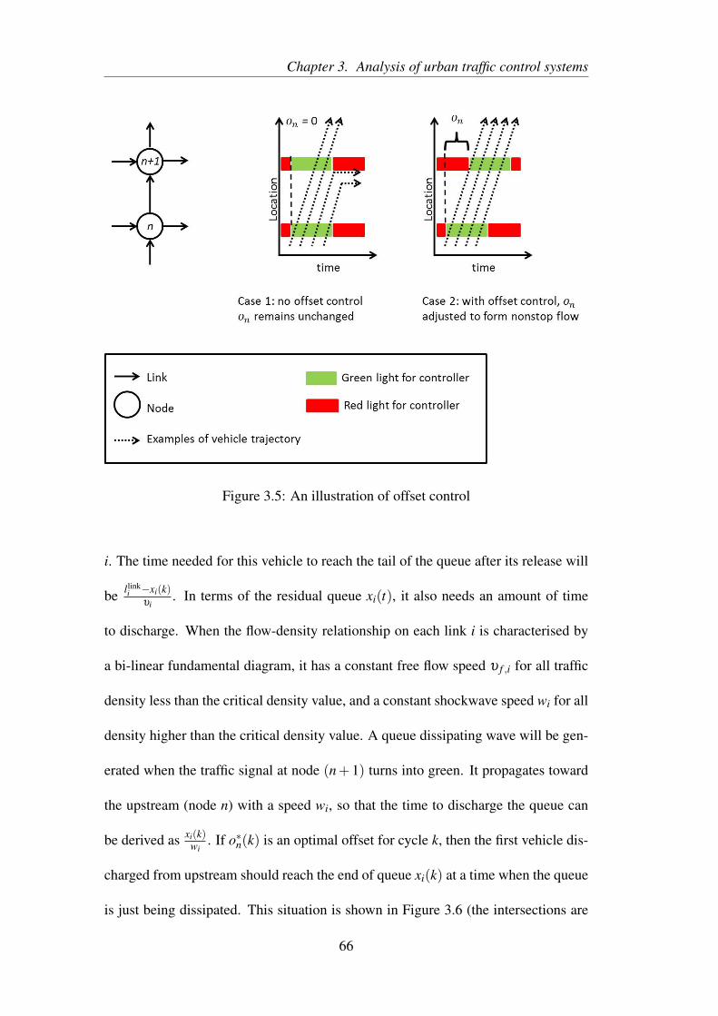
Chapter 3. Analysis of urban traffic control systems
Figure 3.5: An illustration of offset control
i. The time needed for this vehicle to reach the tail of the queue after its release will
be llinki −xi(k)
υi. In terms of the residual queue xi(t), it also needs an amount of time
to discharge. When the flow-density relationship on each link i is characterised by
a bi-linear fundamental diagram, it has a constant free flow speed υ f ,i for all traffic
density less than the critical density value, and a constant shockwave speed wi for all
density higher than the critical density value. A queue dissipating wave will be gen-
erated when the traffic signal at node (n+1) turns into green. It propagates toward
the upstream (node n) with a speed wi, so that the time to discharge the queue can
be derived as xi(k)wi
. If o∗n(k) is an optimal offset for cycle k, then the first vehicle dis-
charged from upstream should reach the end of queue xi(k) at a time when the queue
is just being dissipated. This situation is shown in Figure 3.6 (the intersections are
66
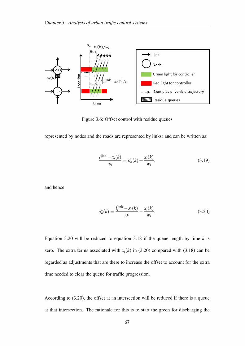
Chapter 3. Analysis of urban traffic control systems
Figure 3.6: Offset control with residue queues
represented by nodes and the roads are represented by links) and can be written as:
llinki − xi(k)
υi= o∗n(k)+
xi(k)wi
, (3.19)
and hence
o∗n(k) =llinki − xi(k)
υi− xi(k)
wi, (3.20)
Equation 3.20 will be reduced to equation 3.18 if the queue length by time k is
zero. The extra terms associated with xi(k) in (3.20) compared with (3.18) can be
regarded as adjustments that are there to increase the offset to account for the extra
time needed to clear the queue for traffic progression.
According to (3.20), the offset at an intersection will be reduced if there is a queue
at that intersection. The rationale for this is to start the green for discharging the
67
Chapter 3. Analysis of urban traffic control systems
local queue at that intersection earlier to create space for the incoming traffic to pro-
ceed without hindrance by the present queue and hence pass through the intersection
without being held by the local queue or red.
Cycle time control
It is known that the capacity of a signal-controlled network depends on its cycle time.
TUC adjusts the cycle times according to the prevailing traffic volume. For example,
one may need to increase cycle times for creating extra operational capacity to cope
with oversaturated traffic. A P-regulator is proposed in [89] for adjusting network-
wide cycle time C(k) over cycle k according to the prevailing traffic:
C(k) =CN +Kc[ξ (k)−ξN ] (3.21)
where CN is a predefined nominal cycle time, ξ (k) = xi(k)xi,max
is the current ratio of
queue length at time k to the link queue capacity, ξ N is a predefined nominal value
for ξ (k). The parameter Kc determines the intensity of the cycle time control. The
control rule (3.21) is also subject to the maximum and minimum bounds on the cycle
times.
3.3.2 Hybrid system
The hybrid system is a variant of the TUC system. As can be seen from (3.7), the
TUC system operates based upon the residual queue measured at the end of each
signal cycle. When a network is oversaturated, TUC works effectively on balancing
68
Chapter 3. Analysis of urban traffic control systems
and dissipating residual queues, as verified by a number of simulation and field tests
(see e.g. [89]). Nevertheless, when the degree of saturation is low, TUC would sim-
ply operate close to the nominal plans gN as the residual queues x are close to zero.
To remedy this, Kouvelas, et al. [90] proposed a hybrid system that runs the TUC
under oversaturated conditions; it switches to a demand-based control mode when
the demands are low. The demand-based control strategy essentially allocates green
splits to the inflow links i according to the corresponding ‘demand-saturation flow’
ratios. This control strategy can be stated as:
gi(k) =hi
∑i∈Iin hi(C−LT ) (3.22)
where hi(k) =qi(k)
Qiis the demand-saturation ratio on link i in cycle k. The objective
here is to balance the degree of saturation which is shown to be an effective way
of operating an intersection [91]. With the demand-based control rule, the hybrid
system operates based upon the measured queue lengths in the following way [90]:
1. if the hybrid controller is in demand-based control mode in cycle k−1, it will
be switched to the TUC control mode in the next cycle k if the queue length
on any one of the inflow links i exceeds a predefined threshold. Otherwise, the
hybrid controller will stay in demand-based mode;
2. if the hybrid controller is in the TUC control mode in cycle k− 1, it will be
switched to demand-based mode in the next cycle k if queue lengths on all
inflow links return below the predefined threshold. Otherwise, the hybrid con-
troller will stay in the TUC mode.
69
Chapter 3. Analysis of urban traffic control systems
3.4 Decentralised control
3.4.1 Max-pressure controller
Max-pressure controller (MP) is a purely decentralised method to control traffic sig-
nals [8] [92]. It was first used for packets transmission in a wireless network [93].
Different from the TUC, it does not require knowledge of network traffic flow and
it operates traffic controllers separately at each intersection. As discussed in [65],
[94], a weakness of the TUC system is that it does not consider explicitly the down-
stream queue constraint and spillover phenomena. The MP controller adjusts local
green splits based on the differences between upstream and downstream local queue
length of each intersection. Given the traffic flowing from an inflow link i to a set of
outflow links Ioutn , where j ∈ Iout
n , through an intersection n, the ‘pressure’ ψi(k) for
this movement over a time period T can be defined as:
ψi =T
∑t=1
Qi
xi(t)− ∑j∈Iout
n
ζi jx j(t)
, (3.23)
where xi is the queue length of the link, Qi is the maximum flow rate of the link. ζi j
is the associated turning ratios for each pair of (i, j). At each signal stage, the inflow
link i which has right of way will be associated with their pressure ψi. The MP con-
troller assigns green light time to the signal stage with the maximum pressure. The
MP is not a cyclic control, so that the controller can allocates more green split to
the links with higher pressure in any sequences. The pseudo code of the non-cyclic
70
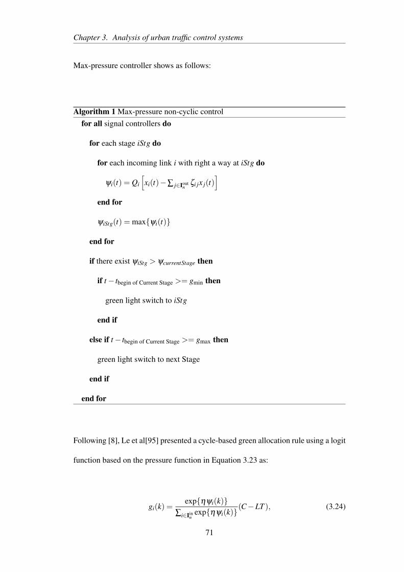
Chapter 3. Analysis of urban traffic control systems
Max-pressure controller shows as follows:
Algorithm 1 Max-pressure non-cyclic controlfor all signal controllers do
for each stage iStg do
for each incoming link i with right a way at iStg do
ψi(t) = Qi
[xi(t)−∑ j∈Iout
nζi jx j(t)
]end for
ψiStg(t) = max{ψi(t)}
end for
if there exist ψiStg > ψcurrentStage then
if t− tbegin of Current Stage >= gmin then
green light switch to iStg
end if
else if t− tbegin of Current Stage >= gmax then
green light switch to next Stage
end if
end for
Following [8], Le et al[95] presented a cycle-based green allocation rule using a logit
function based on the pressure function in Equation 3.23 as:
gi(k) =exp{ηψi(k)}
∑i∈Iinn
exp{ηψi(k)}(C−LT ), (3.24)
71
Chapter 3. Analysis of urban traffic control systems
where gi(k) is the proportion of cycle time allocated to link i among all inflow links
in Iinn during cycle k, η ≥ 0 is a model parameter tuning the sensitivity of green pro-
portion with respect to the pressure. As η tends to zero, the green allocation tends
to uniform. As η tends to ∞, all green will simply be allocated to the link or traffic
movement i with the highest pressure during cycle k [95].
For an intersection that is isolated from any other bottleneck and hence is not subject
to any downstream congestion constraint, the downstream queue term ‘∑ j∈Ioutn
ζi jx j(t)’
in Equation 3.23 will indeed be zero and hence the MP controller will be reduced
to a TUC-like control that operates only based upon local queue and saturation flow
measurements. The major difference between MP and TUC rules is that TUC would
allocate the green according to the predefined nominal green split gN if there is low or
even zero queue detected, while the MP controller will simply allocate the green uni-
formly in the low (or zero) queue circumstance. Moreover, different from the TUC
controller, the derivation of the MP control rule does not require any underlying traf-
fic model and hence the frequency of updating the control policy can theoretically be
flexible, say can range from once a cycle down to every second. It should be noted
that the operation of the MP control does not require any information of network con-
figuration and traffic inflow, and it only requires on-site estimation of queue lengths
which can now be available through various technologies (see e.g. [96]). Regarding
the frequency of updating the control policy, it may be desirable to only update the
MP control once a cycle from a practical perspective. Nevertheless, as [8] points
72
Chapter 3. Analysis of urban traffic control systems
out, updating the control policy only once a cycle may have undesirable outcomes,
say uneven distribution of queues in favour of links with significantly higher demand
[8]. Finally, [8] proves that the MP controller is stabilising (i.e. all queue lengths
are bounded over time) as long as the traffic inflow to each intersection is within the
oversaturation capacity.
The control law (Equation 3.24) determines the green splits at each junction over
cycles. Given the green splits, the MP controller can further regulates the offsets and
network cycle time using the methods described in Sections 3.3.1.
73
Chapter 3. Analysis of urban traffic control systems
3.5 Summary
This chapter analysed a set of different urban traffic systems, starting from cen-
tralised, semi-decentralised, to decentralised. To evaluate their performances, the
systems will be implemented and tested over different network settings in the next
chapter.
One of the chosen centralised control systems is the brute force approach, which
guarantees to find the best solution for the traffic control problem. The optimal solu-
tion is an important benchmark, especially for comparing with solutions of the other
systems in this study. However, the brute force approach is not commonly used
in practice, since the computational time increases exponentially in respect to the
dimensions of the problem and finding the optimal solution can be difficult or not
applicable at all. The other centralised system is the GA, which is a heuristic search
algorithm. Generally, the solution provided by the heuristic algorithm can meet the
practical needs and the algorithm requires less computational time. Nevertheless,
the solution obtained from GA is not a global optimum, and the search in feasible
solutions is randomised.
In terms of the semi-decentralised systems, the TUC system and its modified version
the Hybrid system are presented. TUC is an existing system implemented in real life,
and it is selected in this study to represent a modern urban control system. The TUC
system optimises the green splits and cycle time in a centralised way, while offset
74

Chapter 3. Analysis of urban traffic control systems
control is decentralised. The Hybrid system operates in TUC mode when network is
oversaturated, and switches to a demand-based mode when undersaturated.
Finally, the max-pressure is a decentralised control system proposed in recent years.
It regulates the local green splits according to the local queue lengths at each in-
tersection. Different from the centralised and semi-decentralised systems, the max-
pressure does not require global traffic information and each controller operates sep-
arately.
75
Chapter 4
Comparing centralised and decentralised
traffic control under a macroscopic flow
model
4.1 Introduction
This chapter implements and tests the control systems presented in Chapter 3 over
different networks. This chapter begins with the test of control systems on a one-
way arterial network in Section 4.2. The test extends to a two-way arterial network
in Section 4.3 and a two-dimensional grid network in Section 4.4. Since, the offset
plan is found as a key to bridge the gap between the centralised and the decentralised
control systems, a centralised offset controller is proposed and tested in Section 4.5.
Finally, Section 4.6 is a summary of this chapter.
76
Chapter 4. Test under macroscopic flow model
4.2 One-way arterial network
4.2.1 Network Configurations
Figure 4.1 shows the one-way arterial network considered in this study. It con-
sists of three intersections and ten roads, where the intersections are represented by
nodes and the roads are represented by links. The traffic dynamics are modelled by
the CTM, and the flow-density relationship on each link is described by a bi-linear
fundamental diagram (see Section 2.2.2). The network is discretised into 120 cells
where each cell is 14 metres long. The cell length is calculated from υ∆t, which is
the minimum distance for a vehicle to travel at the free flow speed υ during one time
step ∆t. For each cell c (the CTM model divides links into cells), the free flow speed
υc and shockwave speed wc are set to 50 kph and 16 kph respectively (approximately
equivalent to 30 mph and 10 mph). The speed limit of an urban area commonly is
30 mph, such as London and Paris, and the shockwave speed is calculated basing on
the defined flow-density relationship. In addition, the distance between two succes-
sive nodes for the arterial is set to 160 metres (around 0.1 mile), which is the length
of city blocks seen in New York and Barcelona. By knowing the distance between
two adjacent nodes on the arterial and the free flow speed of the vehicles, the free
flow travel time between the two nodes can be calculated which equals to 12 seconds.
The test scenario is specified by a time horizon, traffic demand profiles and other
settings. The time horizon T of the test is set as 1500 time steps, where one time
step ∆t is one second. The following demand profiles Λx(t) and Λy(t) are assigned
77
Chapter 4. Test under macroscopic flow model
to the horizontal and vertical (cross) streets accordingly:
Λx(t) =
0.6λ , 0≤ t ≤ 300
λ , 301≤ t ≤ 600
0.6λ , 601≤ t ≤ 900
0, t > 900
(4.1)
Λy(t) =
0.48λ , 0≤ t ≤ 300
0.8λ , 301≤ t ≤ 600
0.48λ , 601≤ t ≤ 900
0, t > 900
(4.2)
where λ is a parameter (with unit: [veh/hr]) for tuning the magnitude of demand.
The period from time step 901 to 1500 is regarded as the cooling period in which
no further traffic will be loaded into the network. This cooling period is used to
ensure all traffic can be cleared by the end of test and hence a fair comparison of
performance (in terms of the network delays) of the control systems over all circum-
stances can be obtained. The control systems will be tested over different values of
the parameter λ which represent different levels of demand. To quantify the degree
of congestion, an indicator γ is defined as:
γ =1n
T
∑t=1
C
∑c=1
qc(t)Qc(t)
. (4.3)
78
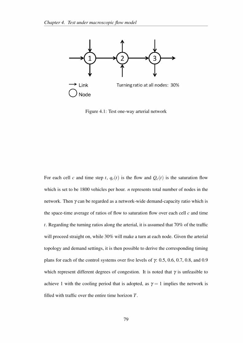
Chapter 4. Test under macroscopic flow model
Figure 4.1: Test one-way arterial network
For each cell c and time step t, qc(t) is the flow and Qc(t) is the saturation flow
which is set to be 1800 vehicles per hour. n represents total number of nodes in the
network. Then γ can be regarded as a network-wide demand-capacity ratio which is
the space-time average of ratios of flow to saturation flow over each cell c and time
t. Regarding the turning ratios along the arterial, it is assumed that 70% of the traffic
will proceed straight on, while 30% will make a turn at each node. Given the arterial
topology and demand settings, it is then possible to derive the corresponding timing
plans for each of the control systems over five levels of γ: 0.5, 0.6, 0.7, 0.8, and 0.9
which represent different degrees of congestion. It is noted that γ is unfeasible to
achieve 1 with the cooling period that is adopted, as γ = 1 implies the network is
filled with traffic over the entire time horizon T .
79
Chapter 4. Test under macroscopic flow model
4.2.2 Settings of the test control systems
To derive the centralised timing plans, a ‘brute force’ solution is computed, which
minimises the total delay on all links by simulating the arterial network over all pos-
sible timing plan settings. The timing plan settings include cycle time, green splits
and offsets. To mimic actual operations, a total of 16 seconds lost time is considered
in each cycle when deriving the timing plan. The green splits and offsets are allowed
to vary every cycle according to the temporal variations in the demand flows. The
workstation used for the tests in this chapter has Intel Xeon E5-2630 v3 2.4GHz
processor and 16GB RAM. The test program is written in Matlab 2013b. The brute
force solution can be regarded as the global optimal plan that minimises the total
arterial delay.It takes 12 hours to complete a brute force search. It is known that the
brute force is rarely used in practice, however, it is a useful benchmark for evalu-
ating the performance of different control systems. Compared with the brute force
solution, another centralised timing plan is also computed by using GA which takes
an hour to solve. Additionally, the offset values at one of the nodes (Node 2) in the
test network remains unchanged through the test (also applies to the decentralised
offset controller); this setting is to make a valid comparison between different offset
controls.
To derive the control timing plans of the semi-decentralised and decentralised sys-
tems, some control parameters need to be specified before conducting the experi-
ment. The nominal green gN in the TUC controller is set according to the estimated
demand-saturation flow ratios as shown in Equation 3.22. Since the centralised sys-
80
Chapter 4. Test under macroscopic flow model
tems are cyclic control, so the decentralised system max-pressure will be using its
cyclic version for comparison. As noted by [95], there is no straightforward way
to determine an optimal value for η in the cyclic MP controller. Consequently, the
value of η is determined by trial-and-error over different settings for the best per-
formance results. It is found that the best value of η will be 0.91, 0.64, 0.61, 0.55,
0.46 for γ equals to 0.5, 0.6, 0.7, 0.8, 0.9 respectively. The finding is not intuitive,
as it implies that the cyclic MP should be made to be less sensitive to the pressure as
the degree of congestion increases. For all of the considered semi-decentralised and
decentralised systems, the control timing plans are derived instantaneously.
4.2.3 Test results
The total network delays delivered by each of the control system are compared and
plotted in Figure 4.2 over different γ . To mimic the effect of imperfect estimation in
traffic flow quantities, all controllers are run over a set of 100 Monte Carlo simula-
tions in which all inflows and turning ratios are incorporated with a Gaussian white
noise with a standard deviation equalling to 10% of the associated expected flow or
split value. Therefore, the delay values plotted in Figure 4.2 are averages produced
by each controller over the 100 Monte Carlo runs. The optimal arterial cycle times
are determined as 54, 80, 80, 92, and 102 seconds for γ = 0.5, 0.6, 0.7, 0.8, and 0.9
respectively.
The centralised system, brute force approach, outperforms all other systems in Fig-
81
Chapter 4. Test under macroscopic flow model
ure 4.2. This is expected while such a brute force solution would take a much longer
time to compute. Interestingly, all semi-decentralised or decentralised systems can
outperform the centralised GA at high γ values, due to the adaptive nature of the de-
centralised systems. Although GA does derive plans that have variable green splits
over different cycles (i.e. the Variable-Green-Fixed-Cycle plan as in [70]), its long
computing time (1-hr) prevents it from being adaptive to prevailing traffic and hence
discounts its effectiveness when subject to the 10% stochastic variations.
In terms of the performance of semi-decentralised and decentralised control systems,
Hybrid controller performs slightly better than TUC under a low degree of conges-
tion (e.g. γ = 0.5 or 0.6). The Hybrid system is structurally the same as TUC except it
will operate in a demand-based mode when the network occupancy is low. With the
low occupancies, the network may not have residue queues being detected at the end
of each cycle and the TUC system behaves similarly to a fixed-time controller (see
the control rule in Equation 3.7). With the demand-based mode, the Hybrid system
still can adapt to the traffic, since its operation is based on the traffic flow rate. With
a high γ value (e.g. 0.8 or 0.9), the arterial is congested and hence the Hybrid system
will be operating in TUC mode most of the time. Consequently, the performances
of the two systems are almost identical. The cyclic MP performs similarly to TUC
and Hybrid. As mentioned, when there is a low (or zero) queue on the downstream
links, the cyclic MP reduces to a TUC-like control.
To gain further insight into the control systems, Figure 4.3 shows the profiles of green
82
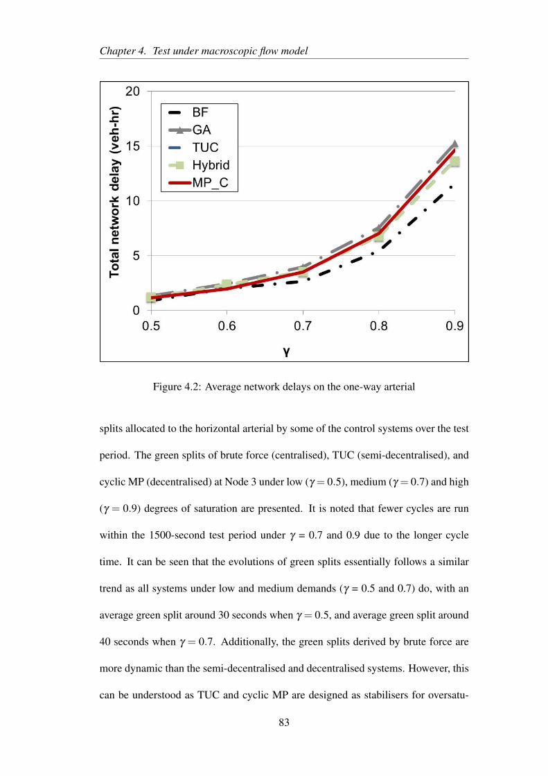
Chapter 4. Test under macroscopic flow model
Figure 4.2: Average network delays on the one-way arterial
splits allocated to the horizontal arterial by some of the control systems over the test
period. The green splits of brute force (centralised), TUC (semi-decentralised), and
cyclic MP (decentralised) at Node 3 under low (γ = 0.5), medium (γ = 0.7) and high
(γ = 0.9) degrees of saturation are presented. It is noted that fewer cycles are run
within the 1500-second test period under γ = 0.7 and 0.9 due to the longer cycle
time. It can be seen that the evolutions of green splits essentially follows a similar
trend as all systems under low and medium demands (γ = 0.5 and 0.7) do, with an
average green split around 30 seconds when γ = 0.5, and average green split around
40 seconds when γ = 0.7. Additionally, the green splits derived by brute force are
more dynamic than the semi-decentralised and decentralised systems. However, this
can be understood as TUC and cyclic MP are designed as stabilisers for oversatu-
83
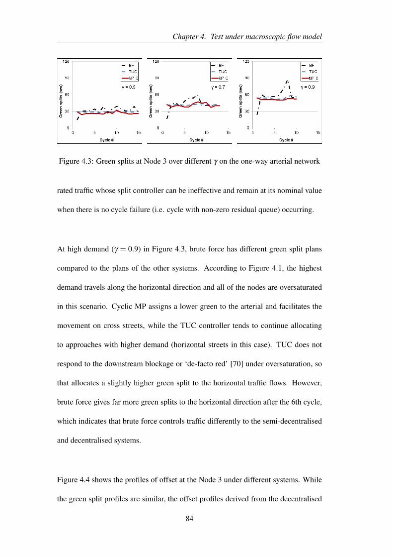
Chapter 4. Test under macroscopic flow model
Figure 4.3: Green splits at Node 3 over different γ on the one-way arterial network
rated traffic whose split controller can be ineffective and remain at its nominal value
when there is no cycle failure (i.e. cycle with non-zero residual queue) occurring.
At high demand (γ = 0.9) in Figure 4.3, brute force has different green split plans
compared to the plans of the other systems. According to Figure 4.1, the highest
demand travels along the horizontal direction and all of the nodes are oversaturated
in this scenario. Cyclic MP assigns a lower green to the arterial and facilitates the
movement on cross streets, while the TUC controller tends to continue allocating
to approaches with higher demand (horizontal streets in this case). TUC does not
respond to the downstream blockage or ‘de-facto red’ [70] under oversaturation, so
that allocates a slightly higher green split to the horizontal traffic flows. However,
brute force gives far more green splits to the horizontal direction after the 6th cycle,
which indicates that brute force controls traffic differently to the semi-decentralised
and decentralised systems.
Figure 4.4 shows the profiles of offset at the Node 3 under different systems. While
the green split profiles are similar, the offset profiles derived from the decentralised
84
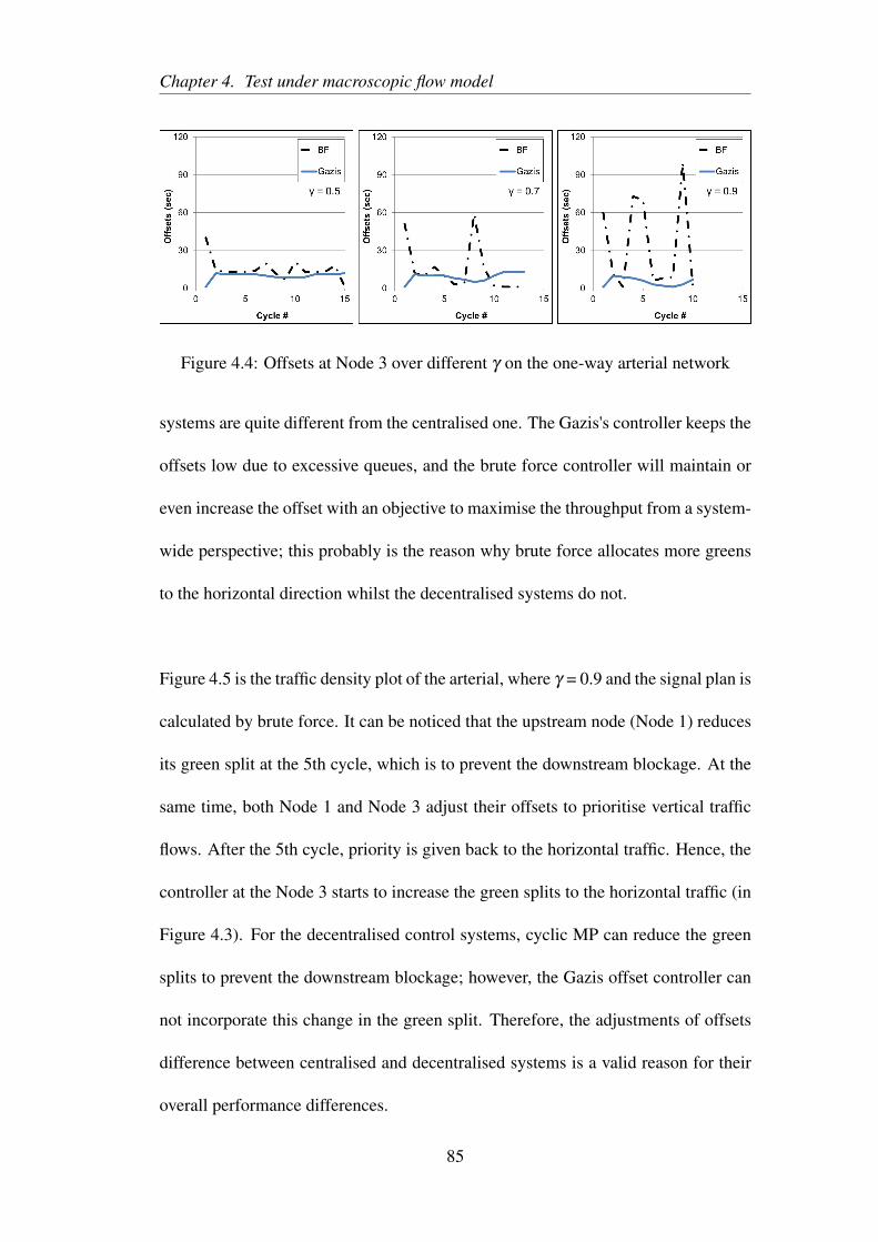
Chapter 4. Test under macroscopic flow model
Figure 4.4: Offsets at Node 3 over different γ on the one-way arterial network
systems are quite different from the centralised one. The Gazis's controller keeps the
offsets low due to excessive queues, and the brute force controller will maintain or
even increase the offset with an objective to maximise the throughput from a system-
wide perspective; this probably is the reason why brute force allocates more greens
to the horizontal direction whilst the decentralised systems do not.
Figure 4.5 is the traffic density plot of the arterial, where γ = 0.9 and the signal plan is
calculated by brute force. It can be noticed that the upstream node (Node 1) reduces
its green split at the 5th cycle, which is to prevent the downstream blockage. At the
same time, both Node 1 and Node 3 adjust their offsets to prioritise vertical traffic
flows. After the 5th cycle, priority is given back to the horizontal traffic. Hence, the
controller at the Node 3 starts to increase the green splits to the horizontal traffic (in
Figure 4.3). For the decentralised control systems, cyclic MP can reduce the green
splits to prevent the downstream blockage; however, the Gazis offset controller can
not incorporate this change in the green split. Therefore, the adjustments of offsets
difference between centralised and decentralised systems is a valid reason for their
overall performance differences.
85
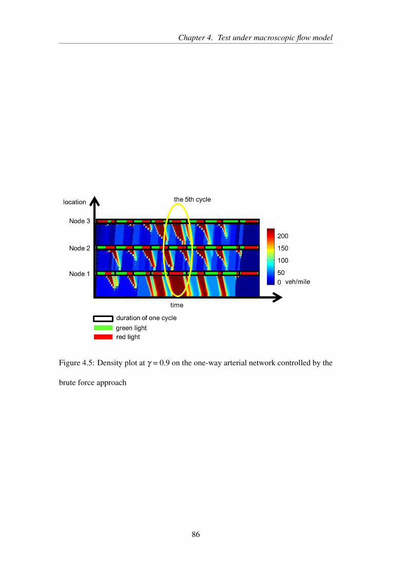
Chapter 4. Test under macroscopic flow model
Figure 4.5: Density plot at γ = 0.9 on the one-way arterial network controlled by the
brute force approach
86
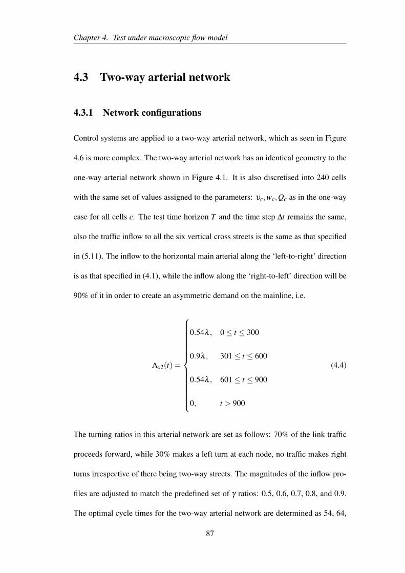
Chapter 4. Test under macroscopic flow model
4.3 Two-way arterial network
4.3.1 Network configurations
Control systems are applied to a two-way arterial network, which as seen in Figure
4.6 is more complex. The two-way arterial network has an identical geometry to the
one-way arterial network shown in Figure 4.1. It is also discretised into 240 cells
with the same set of values assigned to the parameters: υc,wc,Qc as in the one-way
case for all cells c. The test time horizon T and the time step ∆t remains the same,
also the traffic inflow to all the six vertical cross streets is the same as that specified
in (5.11). The inflow to the horizontal main arterial along the ‘left-to-right’ direction
is as that specified in (4.1), while the inflow along the ‘right-to-left’ direction will be
90% of it in order to create an asymmetric demand on the mainline, i.e.
Λx2(t) =
0.54λ , 0≤ t ≤ 300
0.9λ , 301≤ t ≤ 600
0.54λ , 601≤ t ≤ 900
0, t > 900
(4.4)
The turning ratios in this arterial network are set as follows: 70% of the link traffic
proceeds forward, while 30% makes a left turn at each node, no traffic makes right
turns irrespective of there being two-way streets. The magnitudes of the inflow pro-
files are adjusted to match the predefined set of γ ratios: 0.5, 0.6, 0.7, 0.8, and 0.9.
The optimal cycle times for the two-way arterial network are determined as 54, 64,
87
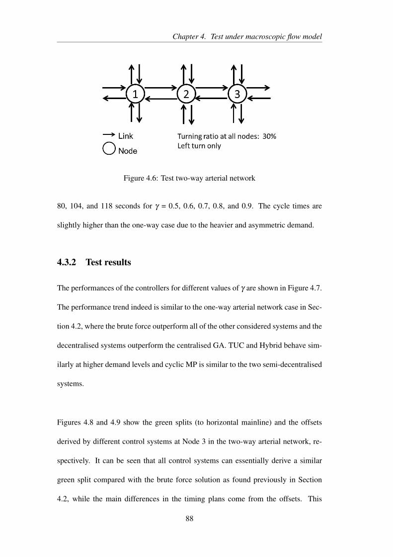
Chapter 4. Test under macroscopic flow model
Figure 4.6: Test two-way arterial network
80, 104, and 118 seconds for γ = 0.5, 0.6, 0.7, 0.8, and 0.9. The cycle times are
slightly higher than the one-way case due to the heavier and asymmetric demand.
4.3.2 Test results
The performances of the controllers for different values of γ are shown in Figure 4.7.
The performance trend indeed is similar to the one-way arterial network case in Sec-
tion 4.2, where the brute force outperform all of the other considered systems and the
decentralised systems outperform the centralised GA. TUC and Hybrid behave sim-
ilarly at higher demand levels and cyclic MP is similar to the two semi-decentralised
systems.
Figures 4.8 and 4.9 show the green splits (to horizontal mainline) and the offsets
derived by different control systems at Node 3 in the two-way arterial network, re-
spectively. It can be seen that all control systems can essentially derive a similar
green split compared with the brute force solution as found previously in Section
4.2, while the main differences in the timing plans come from the offsets. This
88
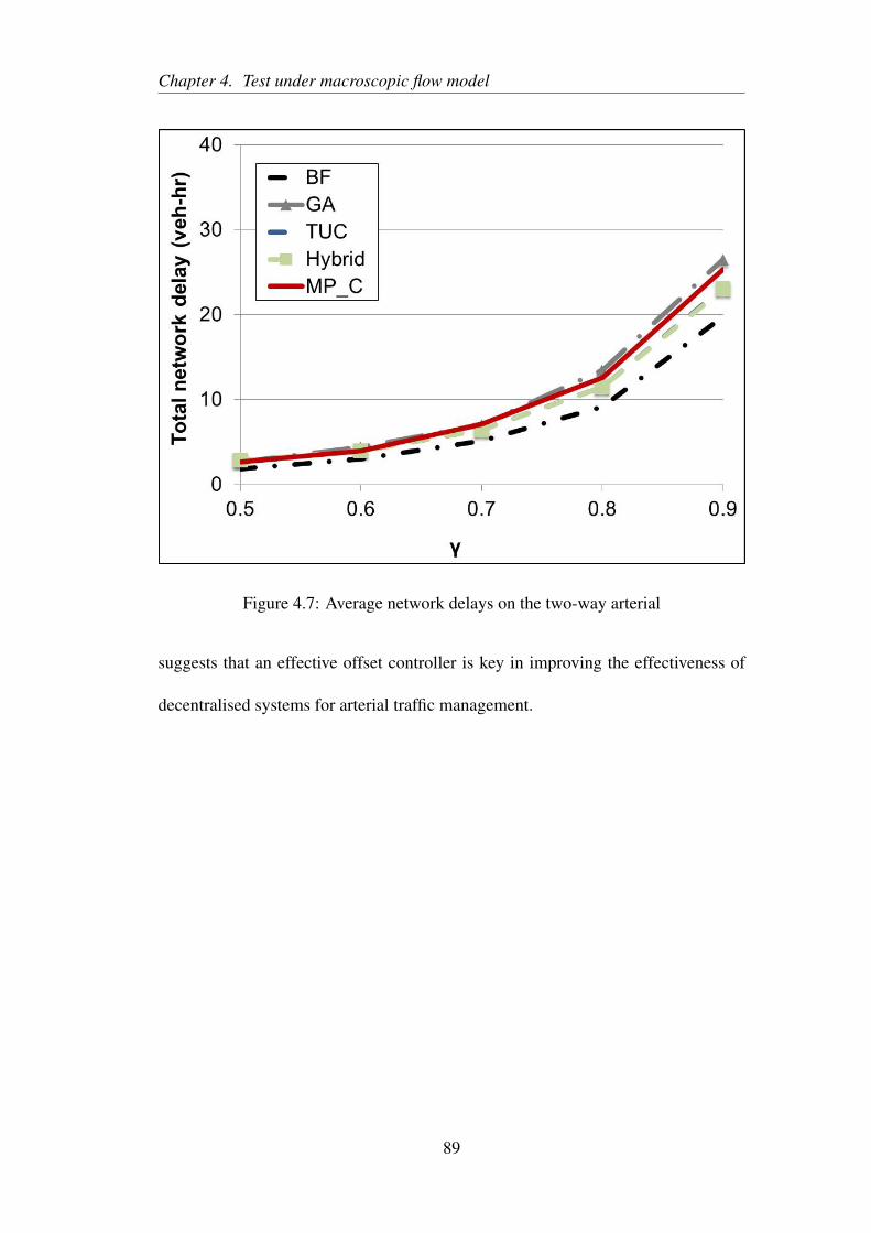
Chapter 4. Test under macroscopic flow model
Figure 4.7: Average network delays on the two-way arterial
suggests that an effective offset controller is key in improving the effectiveness of
decentralised systems for arterial traffic management.
89
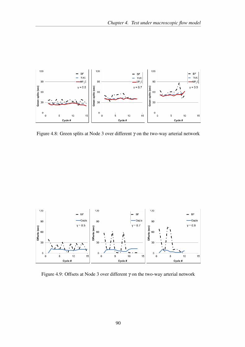
Chapter 4. Test under macroscopic flow model
Figure 4.8: Green splits at Node 3 over different γ on the two-way arterial network
Figure 4.9: Offsets at Node 3 over different γ on the two-way arterial network
90
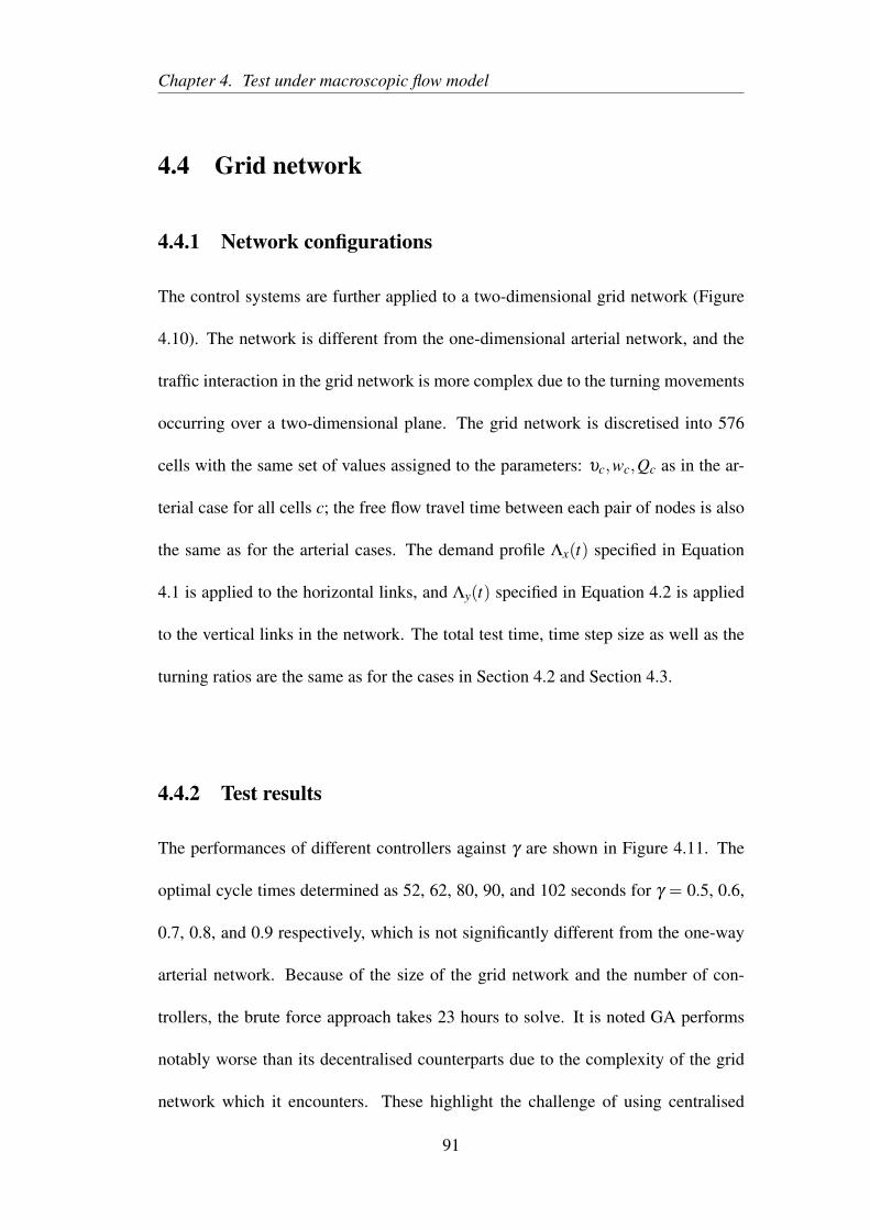
Chapter 4. Test under macroscopic flow model
4.4 Grid network
4.4.1 Network configurations
The control systems are further applied to a two-dimensional grid network (Figure
4.10). The network is different from the one-dimensional arterial network, and the
traffic interaction in the grid network is more complex due to the turning movements
occurring over a two-dimensional plane. The grid network is discretised into 576
cells with the same set of values assigned to the parameters: υc,wc,Qc as in the ar-
terial case for all cells c; the free flow travel time between each pair of nodes is also
the same as for the arterial cases. The demand profile Λx(t) specified in Equation
4.1 is applied to the horizontal links, and Λy(t) specified in Equation 4.2 is applied
to the vertical links in the network. The total test time, time step size as well as the
turning ratios are the same as for the cases in Section 4.2 and Section 4.3.
4.4.2 Test results
The performances of different controllers against γ are shown in Figure 4.11. The
optimal cycle times determined as 52, 62, 80, 90, and 102 seconds for γ = 0.5, 0.6,
0.7, 0.8, and 0.9 respectively, which is not significantly different from the one-way
arterial network. Because of the size of the grid network and the number of con-
trollers, the brute force approach takes 23 hours to solve. It is noted GA performs
notably worse than its decentralised counterparts due to the complexity of the grid
network which it encounters. These highlight the challenge of using centralised
91
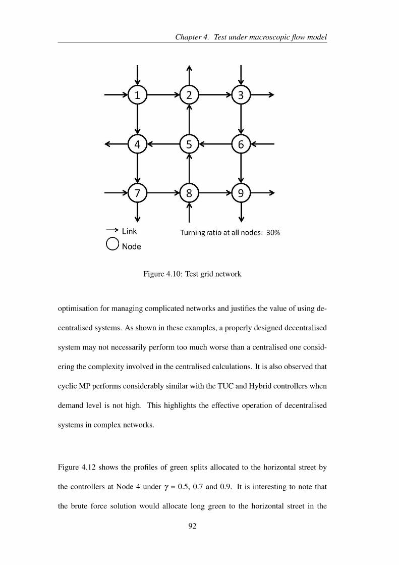
Chapter 4. Test under macroscopic flow model
Figure 4.10: Test grid network
optimisation for managing complicated networks and justifies the value of using de-
centralised systems. As shown in these examples, a properly designed decentralised
system may not necessarily perform too much worse than a centralised one consid-
ering the complexity involved in the centralised calculations. It is also observed that
cyclic MP performs considerably similar with the TUC and Hybrid controllers when
demand level is not high. This highlights the effective operation of decentralised
systems in complex networks.
Figure 4.12 shows the profiles of green splits allocated to the horizontal street by
the controllers at Node 4 under γ = 0.5, 0.7 and 0.9. It is interesting to note that
the brute force solution would allocate long green to the horizontal street in the
92
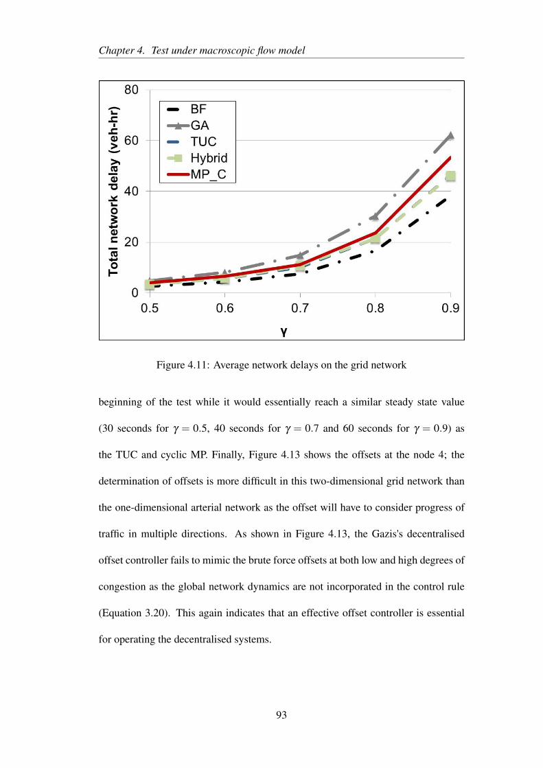
Chapter 4. Test under macroscopic flow model
Figure 4.11: Average network delays on the grid network
beginning of the test while it would essentially reach a similar steady state value
(30 seconds for γ = 0.5, 40 seconds for γ = 0.7 and 60 seconds for γ = 0.9) as
the TUC and cyclic MP. Finally, Figure 4.13 shows the offsets at the node 4; the
determination of offsets is more difficult in this two-dimensional grid network than
the one-dimensional arterial network as the offset will have to consider progress of
traffic in multiple directions. As shown in Figure 4.13, the Gazis's decentralised
offset controller fails to mimic the brute force offsets at both low and high degrees of
congestion as the global network dynamics are not incorporated in the control rule
(Equation 3.20). This again indicates that an effective offset controller is essential
for operating the decentralised systems.
93
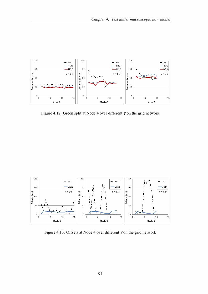
Chapter 4. Test under macroscopic flow model
Figure 4.12: Green split at Node 4 over different γ on the grid network
Figure 4.13: Offsets at Node 4 over different γ on the grid network
94
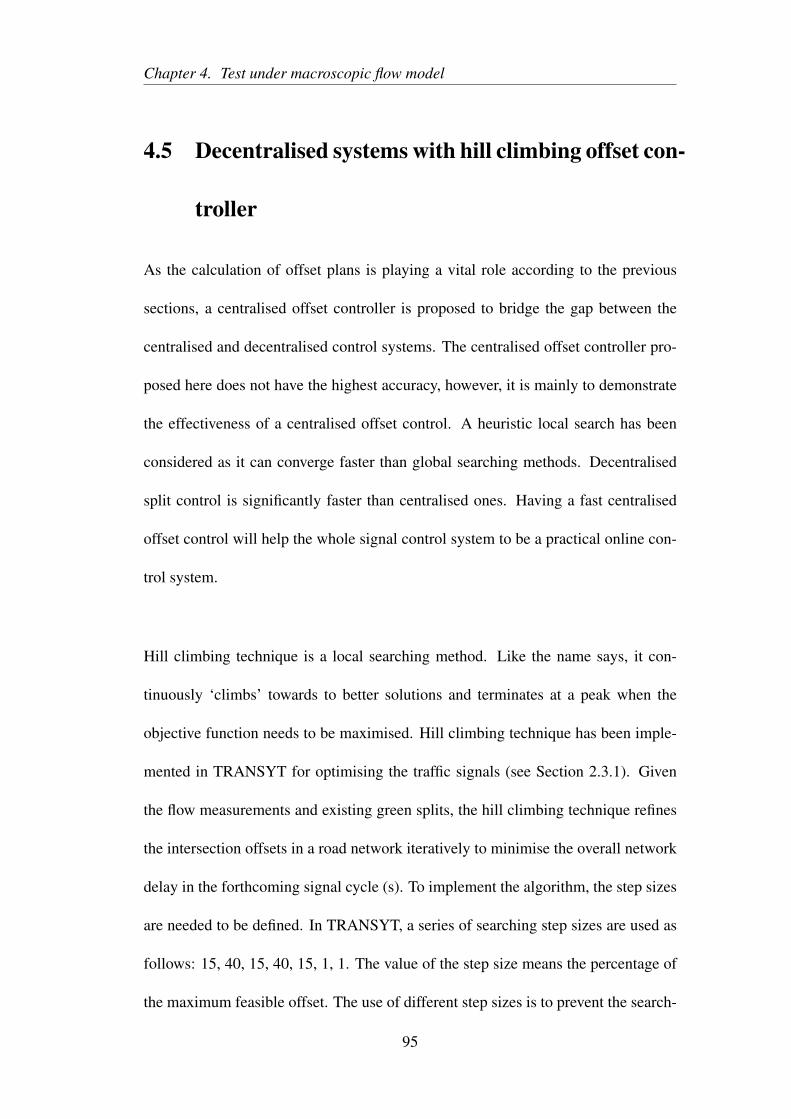
Chapter 4. Test under macroscopic flow model
4.5 Decentralised systems with hill climbing offset con-
troller
As the calculation of offset plans is playing a vital role according to the previous
sections, a centralised offset controller is proposed to bridge the gap between the
centralised and decentralised control systems. The centralised offset controller pro-
posed here does not have the highest accuracy, however, it is mainly to demonstrate
the effectiveness of a centralised offset control. A heuristic local search has been
considered as it can converge faster than global searching methods. Decentralised
split control is significantly faster than centralised ones. Having a fast centralised
offset control will help the whole signal control system to be a practical online con-
trol system.
Hill climbing technique is a local searching method. Like the name says, it con-
tinuously ‘climbs’ towards to better solutions and terminates at a peak when the
objective function needs to be maximised. Hill climbing technique has been imple-
mented in TRANSYT for optimising the traffic signals (see Section 2.3.1). Given
the flow measurements and existing green splits, the hill climbing technique refines
the intersection offsets in a road network iteratively to minimise the overall network
delay in the forthcoming signal cycle (s). To implement the algorithm, the step sizes
are needed to be defined. In TRANSYT, a series of searching step sizes are used as
follows: 15, 40, 15, 40, 15, 1, 1. The value of the step size means the percentage of
the maximum feasible offset. The use of different step sizes is to prevent the search-
95
Chapter 4. Test under macroscopic flow model
ing algorithm from being trapped into a local minimum. With this sequence, the
offset value is first increased at a specific node in the road network by ‘15%’ (first
entry ‘15’ in the sequence), and then determines the corresponding change in total
network delay by re-running the test with this revised offset. If this gives a reduc-
tion in the delay, the offset value will continue to be increased, this time by ‘40%’
(second entry ‘40’ in the sequence); otherwise, the offset value will be reduced by
40% and see whether it will bring a reduction in total network delay. The algorithm
proceeds with this predefined step size sequence until the sequence is exhausted or
if there is no further reduction in total network delay achievable. The algorithm then
moves on to the second node in the network, repeating the process until all nodes in
the network have been visited. Figure 4.14 shows the procedure of the hill climbing
offset control in a flowchart format.
A sensitivity analysis has been carried out for examining the choices of the searching
step sizes. The analysis considered the two test networks from the previous sections
(Section 4.2 and 4.4): one-way arterial network and 3 by 3 grid network. The tests
have carried out with different searching step sizes for offset control. Figure 4.15
shows the average impacts of the step sizes on the network delay. The x-axis is the
step size over the searching range, and the y-axis is the scaled performance to the
minimum to maximum network delays in the results. For example, when the scaled
performance equals 0, it means the performance is the lowest network delay founded
in the test. On the other hand, the scaled performance equals to 1 when the result is
the highest network delay founded in the test. When the step size larger than 50% of
96
Chapter 4. Test under macroscopic flow model
the searching range, there are much less offset values can be visited. This is why the
corresponding network delays cannot outperform the results in smaller step sizes.
Smaller step sizes lead to better performance, however, will have more offset values
need to visit and will take longer time. According to the Figure 4.15, any values less
than 20% of the searching range can find better results than any larger step sizes. In
this case, the 15% step size looks reasonable and any step size around it gives sim-
ilar results. Alternatively using the step size 40% and 15% can avoid the algorithm
trapped in one local optimal. Leaving the smallest step size (1%) at the end of the
searching process is to explore its direct neighbourhood.
Figures 4.16, 4.17 and 4.18 show the performance of the offset controller in the one-
way arterial network, the two-way arterial network and the grid network respectively.
With the consideration of the performance shown in the previous sections, the focus
of this section is on the cyclic MP and replaces the Gazis offset controller with the
hill climbing based offset controller. The results show that the offsets determined
by the centralised hill climbing algorithm improve the performance of the cyclic
MP. Different from the brute force and GA approach, this proposed controller only
needs to perform a centralised optimisation to calculate the offsets, while the green
splits can be determined through the decentralised MP approach. Consequently, a
considerable amount of computational effort can be saved and a similar centralised
performance can still be achieved. The saving in computational effort will be even
more significant in large networks as it is known that the complexity of the signal op-
timisation problem grows exponentially with the number of nodes involved. In this
97

Chapter 4. Test under macroscopic flow model
specific example, it takes 40 seconds to compute all offsets for the arterial network
and 65 seconds for the grid network on a computer (Intel i5-4370 CPU 3.2GHz). The
results are promising as they reveal the possibility of using decentralised systems for
effective network-wide real-time urban traffic control.
98
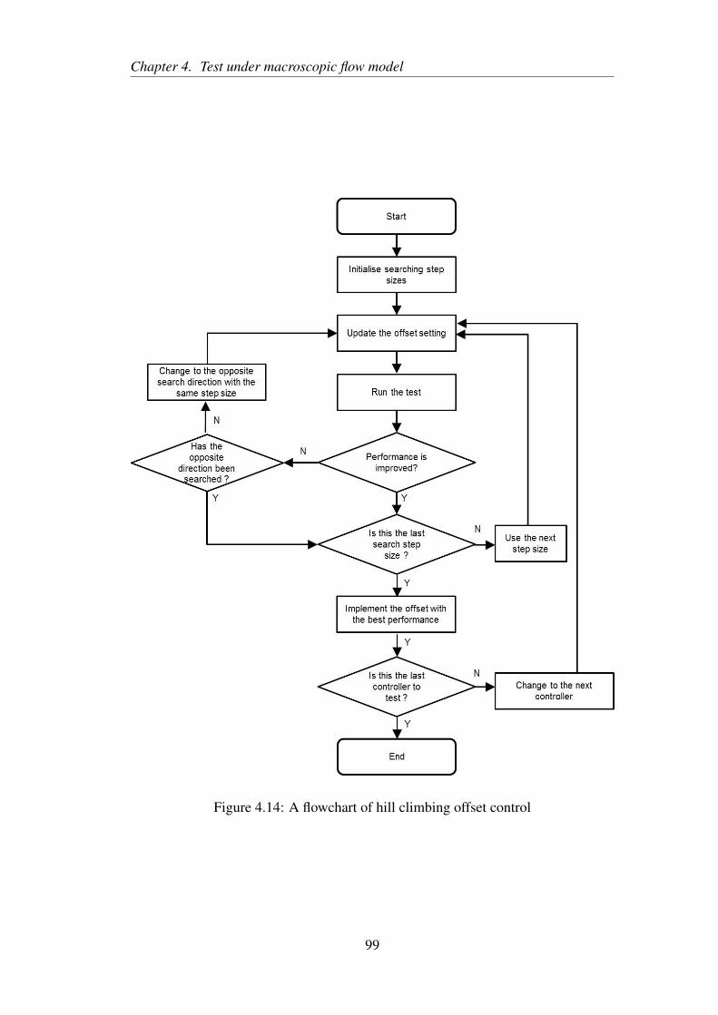
Chapter 4. Test under macroscopic flow model
Figure 4.14: A flowchart of hill climbing offset control
99
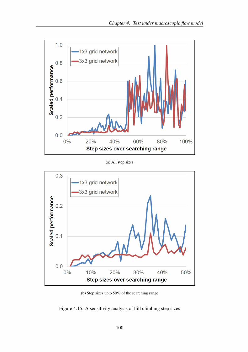
Chapter 4. Test under macroscopic flow model
(a) All step sizes
(b) Step sizes upto 50% of the searching range
Figure 4.15: A sensitivity analysis of hill climbing step sizes
100
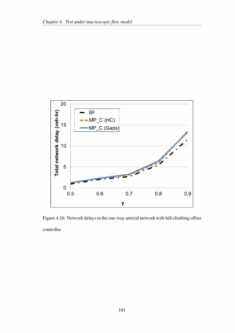
Chapter 4. Test under macroscopic flow model
Figure 4.16: Network delays in the one-way arterial network with hill climbing offset
controller
101
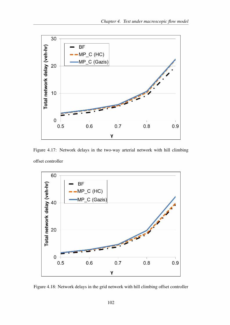
Chapter 4. Test under macroscopic flow model
Figure 4.17: Network delays in the two-way arterial network with hill climbing
offset controller
Figure 4.18: Network delays in the grid network with hill climbing offset controller
102
Chapter 4. Test under macroscopic flow model
4.6 Summary
This chapter compared the performances of the control systems: centralised (brute
force approach and GA), semi-decentralised (TUC and Hybrid) and decentralised
(MP) under one-way arterial, two-way arterial, and grid networks.
In terms of the system performances, the performance differences are not significant
before the test networks reach their saturation limits (see Figure 4.2, 4.7 and 4.11).
As expected, the brute force approach outperforms all the other control systems.
However, the GA is not quite efficient as the control timing plans derived by GA are
not adaptive to the stochastic variations in traffic demands. TUC and Hybrid have
very close performances. The cyclic MP performs similar with TUC and Hybrid in
the arterial networks, but not in the grid network. This shows the advantage of the
centralised feature in the TUC system.
To find the insights of the performance differences among the control systems, the
derived green splits and offsets by the control systems are presented in the test results
of each section. The control timing plans show that the corresponding local green
splits determined from centralised, semi-decentralised and decentralised systems are
indeed similar. This implies most benefit gained from centralised control comes
from the setting of offsets. The major challenge of the decentralised offset control
comes when the test network is oversaturated and the controllers are applied to com-
plicated networks, like the grid network adopted in this study. In those cases, offsets
103
Chapter 4. Test under macroscopic flow model
have to be adjusted frequently and accurately in order to balance the progression of
traffic along different directions through the network. To address the problem, a cen-
tralised hill climbing based offset controller is further purposed and integrated with
the decentralised control systems. The results suggest that such a centralised offset
controller helps to reduce the performance gap between centralised and decentralised
systems, and has significantly less computational effort compared to full centralised
systems. Therefore, the proposed centralised offset controller can be extended to de-
sign an efficient decentralised control system. Moreover, the experiments'result are
going to be validated by using a different microscopic traffic flow model SUMO in
the next Chapter 5. With the microscopic model, more detailed vehicle's movements
(such as acceleration and rerouting behaviours) can be captured.
104
Chapter 5
Comparing centralised and decentralised
traffic control under a microscopic flow
model with traffic rerouting
5.1 Introduction
This chapter tests the performance of the centralised and decentralised traffic con-
trols on a microscopic platform with open source SUMO package. Comparing to the
macroscopic CTM in previous chapter 4, SUMO can capture more detailed vehicle
movements and allows vehicles to reroute according to real-time traffic conditions.
The flow model of SUMO is first introduced in Section 5.2 and compared with CTM
model. Both centralised and decentralised control systems are tested with SUMO on
an arterial network in Section 5.3. Rerouting control is introduced and tested on a
grid network in Section 5.4. At the end, Section 5.5 summarises the chapter.
105
Chapter 5. Test under microscopic flow model and traffic rerouting
5.2 Simulation of urban mobility - SUMO
Simulation of urban mobility (SUMO) is an open source traffic simulation platform
developed by German Aerospace Centre (DLR). It is a tool for transport planning,
and can examine the impact of road layout change, new speed limit implementation
or other design adjustments of transport facilities. The simulation is done at micro-
scopic level, where the different modes of transport such as vehicles, pedestrian and
public transport are modelled together. The open source feature benefits users from
spending time to develop their own simulator for test purpose. The results of SUMO
have also become comparable between users [97].
The basic usage of SUMO platform can be divided into three parts: network gen-
eration, demand modelling and simulation [98]. Network can be created in an ap-
plication tool NETCOVERT which comes with SUMO, or can be imported from
online resources (such as OpenStreetMap) and from other simulation platforms (for
instance, VISIM, VISSIM and MATsim). SUMO accepts a wide range of demand
types. For example, the traffic demand can be defined by origin and destination
data, can be generated by traffic flow and turning ratio and can be defined by the trip
routes. In terms of the simulation, the default microscopic flow model of SUMO is
a safety-distance model developed by Krauss [99], and a detailed explanation is in
Section 5.2.1.
106
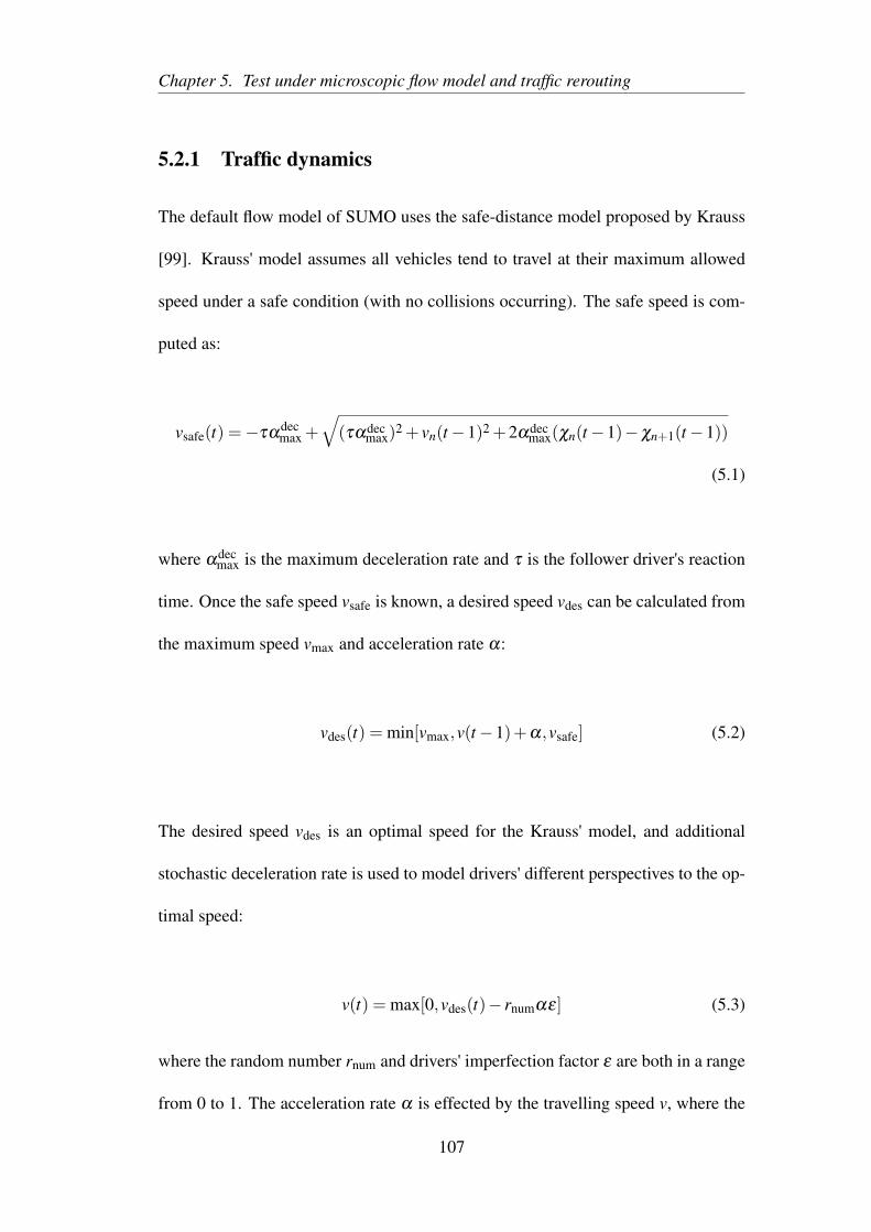
Chapter 5. Test under microscopic flow model and traffic rerouting
5.2.1 Traffic dynamics
The default flow model of SUMO uses the safe-distance model proposed by Krauss
[99]. Krauss' model assumes all vehicles tend to travel at their maximum allowed
speed under a safe condition (with no collisions occurring). The safe speed is com-
puted as:
vsafe(t) =−ταdecmax +
√(ταdec
max)2 + vn(t−1)2 +2αdec
max(χn(t−1)−χn+1(t−1))
(5.1)
where αdecmax is the maximum deceleration rate and τ is the follower driver's reaction
time. Once the safe speed vsafe is known, a desired speed vdes can be calculated from
the maximum speed vmax and acceleration rate α:
vdes(t) = min[vmax,v(t−1)+α,vsafe] (5.2)
The desired speed vdes is an optimal speed for the Krauss' model, and additional
stochastic deceleration rate is used to model drivers' different perspectives to the op-
timal speed:
v(t) = max[0,vdes(t)− rnumαε] (5.3)
where the random number rnum and drivers' imperfection factor ε are both in a range
from 0 to 1. The acceleration rate α is effected by the travelling speed v, where the
107
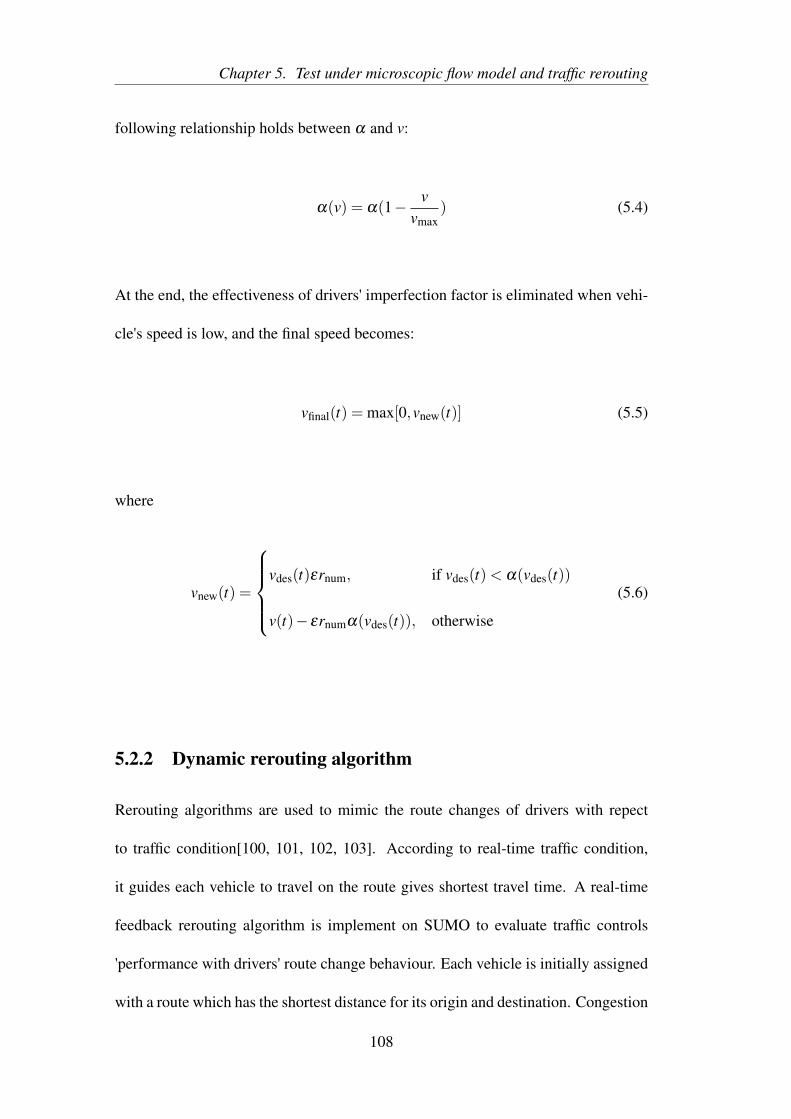
Chapter 5. Test under microscopic flow model and traffic rerouting
following relationship holds between α and v:
α(v) = α(1− vvmax
) (5.4)
At the end, the effectiveness of drivers' imperfection factor is eliminated when vehi-
cle's speed is low, and the final speed becomes:
vfinal(t) = max[0,vnew(t)] (5.5)
where
vnew(t) =
vdes(t)εrnum, if vdes(t)< α(vdes(t))
v(t)− εrnumα(vdes(t)), otherwise
(5.6)
5.2.2 Dynamic rerouting algorithm
Rerouting algorithms are used to mimic the route changes of drivers with repect
to traffic condition[100, 101, 102, 103]. According to real-time traffic condition,
it guides each vehicle to travel on the route gives shortest travel time. A real-time
feedback rerouting algorithm is implement on SUMO to evaluate traffic controls
'performance with drivers' route change behaviour. Each vehicle is initially assigned
with a route which has the shortest distance for its origin and destination. Congestion
108
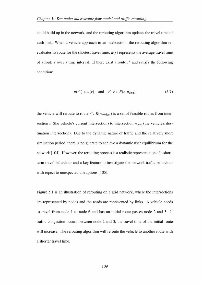
Chapter 5. Test under microscopic flow model and traffic rerouting
could build up in the network, and the rerouting algorithm updates the travel time of
each link. When a vehicle approach to an intersection, the rerouting algorithm re-
evaluates its route for the shortest travel time. u(r) represents the average travel time
of a route r over a time interval. If there exist a route r∗ and satisfy the following
condition:
u(r∗)< u(r) and r∗,r ∈ R(n,ndest) (5.7)
the vehicle will reroute to route r∗. R(n,ndest) is a set of feasible routes from inter-
section n (the vehicle's current intersection) to intersection ndest (the vehicle's des-
tination intersection). Due to the dynamic nature of traffic and the relatively short
simluation period, there is no guarate to achieve a dynamic user equilibrium for the
network [104]. However, the rerouting process is a realistic representation of a short-
term travel behaviour and a key feature to investigate the network traffic behaviour
with repect to unexpected disruptions [105].
Figure 5.1 is an illustration of rerouting on a grid network, where the intersections
are represented by nodes and the roads are represented by links. A vehicle needs
to travel from node 1 to node 6 and has an initial route passes node 2 and 3. If
traffic congestion occurs between node 2 and 3, the travel time of the initial route
will increase. The rerouting algorithm will reroute the vehicle to another route with
a shorter travel time.
109
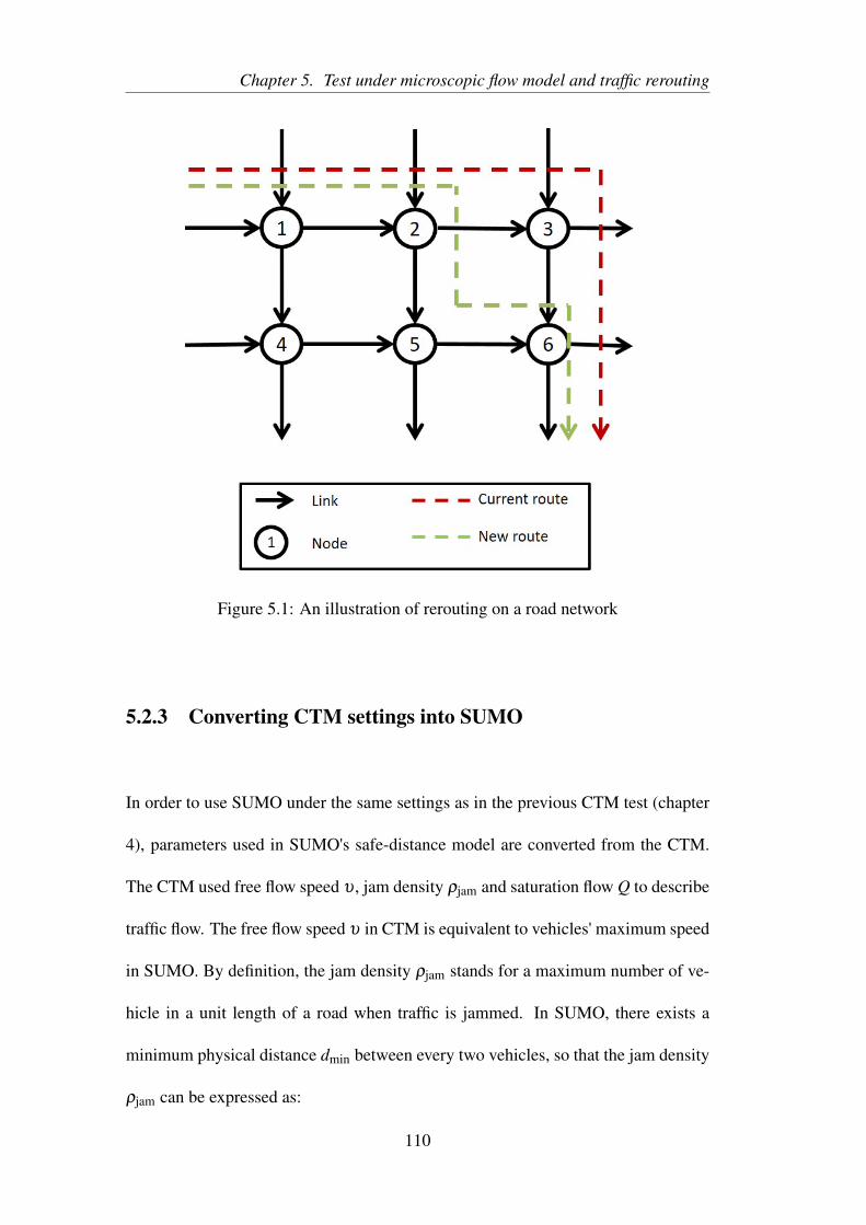
Chapter 5. Test under microscopic flow model and traffic rerouting
Figure 5.1: An illustration of rerouting on a road network
5.2.3 Converting CTM settings into SUMO
In order to use SUMO under the same settings as in the previous CTM test (chapter
4), parameters used in SUMO's safe-distance model are converted from the CTM.
The CTM used free flow speed υ , jam density ρjam and saturation flow Q to describe
traffic flow. The free flow speed υ in CTM is equivalent to vehicles' maximum speed
in SUMO. By definition, the jam density ρjam stands for a maximum number of ve-
hicle in a unit length of a road when traffic is jammed. In SUMO, there exists a
minimum physical distance dmin between every two vehicles, so that the jam density
ρjam can be expressed as:
110
Chapter 5. Test under microscopic flow model and traffic rerouting
ρjam =1
dmin + lveh (5.8)
where lveh is mean vehicle length. In terms of the saturation flow Q, it is the maxi-
mum number of vehicle passed a location in a unit of time. If the time for a vehicle
to pass a location is lveh
v and the time gap between every two vehicles is driver's re-
action time τ , the saturation flow Q can be converted as:
Q =1
τ + lveh
v
(5.9)
The jam density ρjam, saturation flow Q and free flow speed υf were set to be 230
vehicles per mile, 1800 vehicles per hour and 30 mph for CTM tests. Equivalently,
the drivers' reaction time, minimum vehicle distance and vehicle length are set to 1.6
seconds, 2 metres and 5 metres. In addition, SUMO captures the individual move-
ments of each vehicle. The acceleration and deceleration of vehicles are considered
and are set to be 2.6 m2/s and 4.5 m2/s respectively.
In order to visualise the difference between the two flow models, the models are
tested on a single intersection network where the network includes one signal con-
troller and a single road. Only SUMO captures vehicles' acceleration and decelera-
tion. In this case, two SUMO models are tested to compare with CTM, where one
has acceleration and deceleration constraints (SUMO) and the other one does not
have (SUMO (max)). Figure 5.2 and 5.3 show the cumulative arrival and departure
111
Chapter 5. Test under microscopic flow model and traffic rerouting
Figure 5.2: Arrival and departure curves of CTM and SUMO when undersaturated
curves of traffic in undersaturated and oversaturated scenarios. It can be seen that
all flow models have the similar departure curves when traffic is less saturated. The
default SUMO (with consideration of vehicles' acceleration and deceleration) has a
steeper departure curve, which means there are less vehicles left the road every cycle.
The acceleration constraint affects vehicles' departure. In CTM and SUMO (max),
vehicles can accelerate to their maximum speed immediately when the traffic light
turns to green. Figure 5.4 and 5.5 are the network delay results of this comparison
test. The use of the acceleration constraint also lead to a higher network delay in the
default SUMO.
112
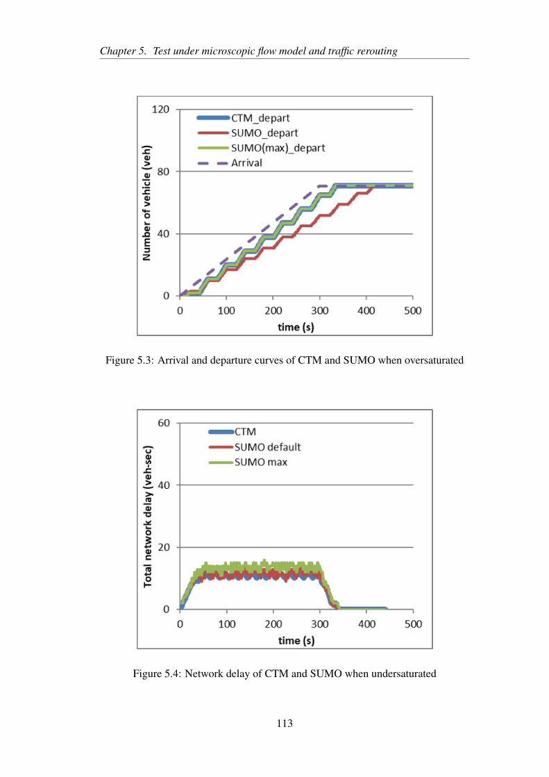
Chapter 5. Test under microscopic flow model and traffic rerouting
Figure 5.3: Arrival and departure curves of CTM and SUMO when oversaturated
Figure 5.4: Network delay of CTM and SUMO when undersaturated
113
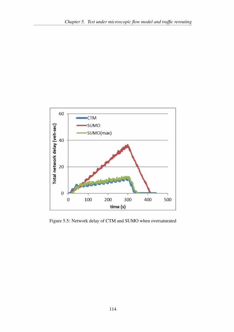
Chapter 5. Test under microscopic flow model and traffic rerouting
Figure 5.5: Network delay of CTM and SUMO when oversaturated
114
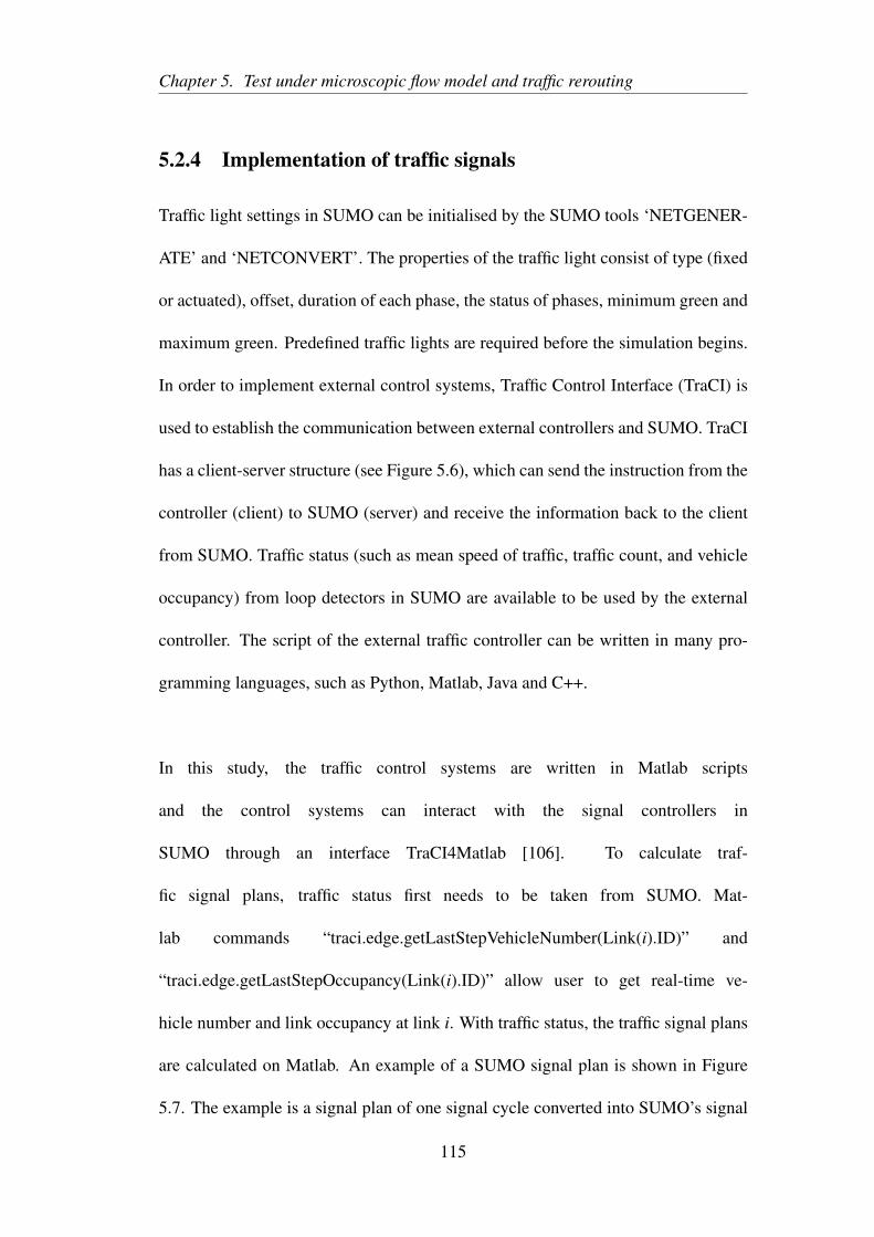
Chapter 5. Test under microscopic flow model and traffic rerouting
5.2.4 Implementation of traffic signals
Traffic light settings in SUMO can be initialised by the SUMO tools ‘NETGENER-
ATE’ and ‘NETCONVERT’. The properties of the traffic light consist of type (fixed
or actuated), offset, duration of each phase, the status of phases, minimum green and
maximum green. Predefined traffic lights are required before the simulation begins.
In order to implement external control systems, Traffic Control Interface (TraCI) is
used to establish the communication between external controllers and SUMO. TraCI
has a client-server structure (see Figure 5.6), which can send the instruction from the
controller (client) to SUMO (server) and receive the information back to the client
from SUMO. Traffic status (such as mean speed of traffic, traffic count, and vehicle
occupancy) from loop detectors in SUMO are available to be used by the external
controller. The script of the external traffic controller can be written in many pro-
gramming languages, such as Python, Matlab, Java and C++.
In this study, the traffic control systems are written in Matlab scripts
and the control systems can interact with the signal controllers in
SUMO through an interface TraCI4Matlab [106]. To calculate traf-
fic signal plans, traffic status first needs to be taken from SUMO. Mat-
lab commands “traci.edge.getLastStepVehicleNumber(Link(i).ID)” and
“traci.edge.getLastStepOccupancy(Link(i).ID)” allow user to get real-time ve-
hicle number and link occupancy at link i. With traffic status, the traffic signal plans
are calculated on Matlab. An example of a SUMO signal plan is shown in Figure
5.7. The example is a signal plan of one signal cycle converted into SUMO’s signal
115
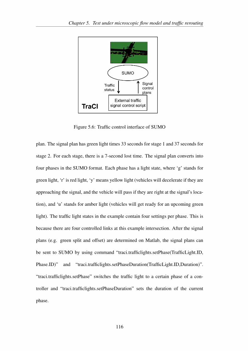
Chapter 5. Test under microscopic flow model and traffic rerouting
Figure 5.6: Traffic control interface of SUMO
plan. The signal plan has green light times 33 seconds for stage 1 and 37 seconds for
stage 2. For each stage, there is a 7-second lost time. The signal plan converts into
four phases in the SUMO format. Each phase has a light state, where ‘g’ stands for
green light, ‘r’ is red light, ‘y’ means yellow light (vehicles will decelerate if they are
approaching the signal, and the vehicle will pass if they are right at the signal’s loca-
tion), and ‘u’ stands for amber light (vehicles will get ready for an upcoming green
light). The traffic light states in the example contain four settings per phase. This is
because there are four controlled links at this example intersection. After the signal
plans (e.g. green split and offset) are determined on Matlab, the signal plans can
be sent to SUMO by using command “traci.trafficlights.setPhase(TrafficLight.ID,
Phase.ID)” and “traci.trafficlights.setPhaseDuration(TrafficLight.ID,Duration)”.
“traci.trafficlights.setPhase” switches the traffic light to a certain phase of a con-
troller and “traci.trafficlights.setPhaseDuration” sets the duration of the current
phase.
116
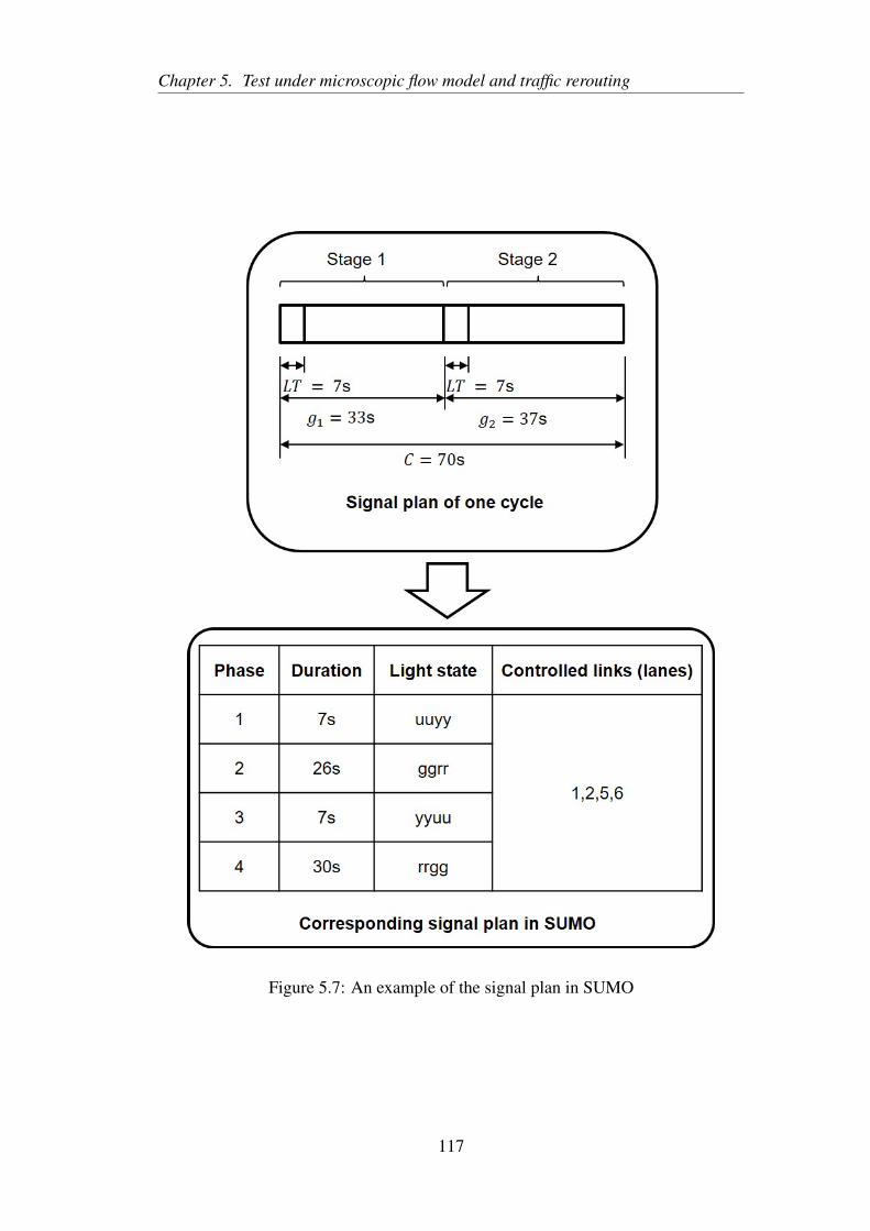
Chapter 5. Test under microscopic flow model and traffic rerouting
Figure 5.7: An example of the signal plan in SUMO
117
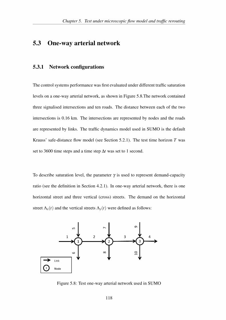
Chapter 5. Test under microscopic flow model and traffic rerouting
5.3 One-way arterial network
5.3.1 Network configurations
The control systems performance was first evaluated under different traffic saturation
levels on a one-way arterial network, as shown in Figure 5.8.The network contained
three signalised intersections and ten roads. The distance between each of the two
intersections is 0.16 km. The intersections are represented by nodes and the roads
are represented by links. The traffic dynamics model used in SUMO is the default
Krauss’ safe-distance flow model (see Section 5.2.1). The test time horizon T was
set to 3600 time steps and a time step ∆t was set to 1 second.
To describe saturation level, the parameter γ is used to represent demand-capacity
ratio (see the definition in Section 4.2.1). In one-way arterial network, there is one
horizontal street and three vertical (cross) streets. The demand on the horizontal
street Λx(t) and the vertical streets Λy(t) were defined as follows:
Figure 5.8: Test one-way arterial network used in SUMO
118
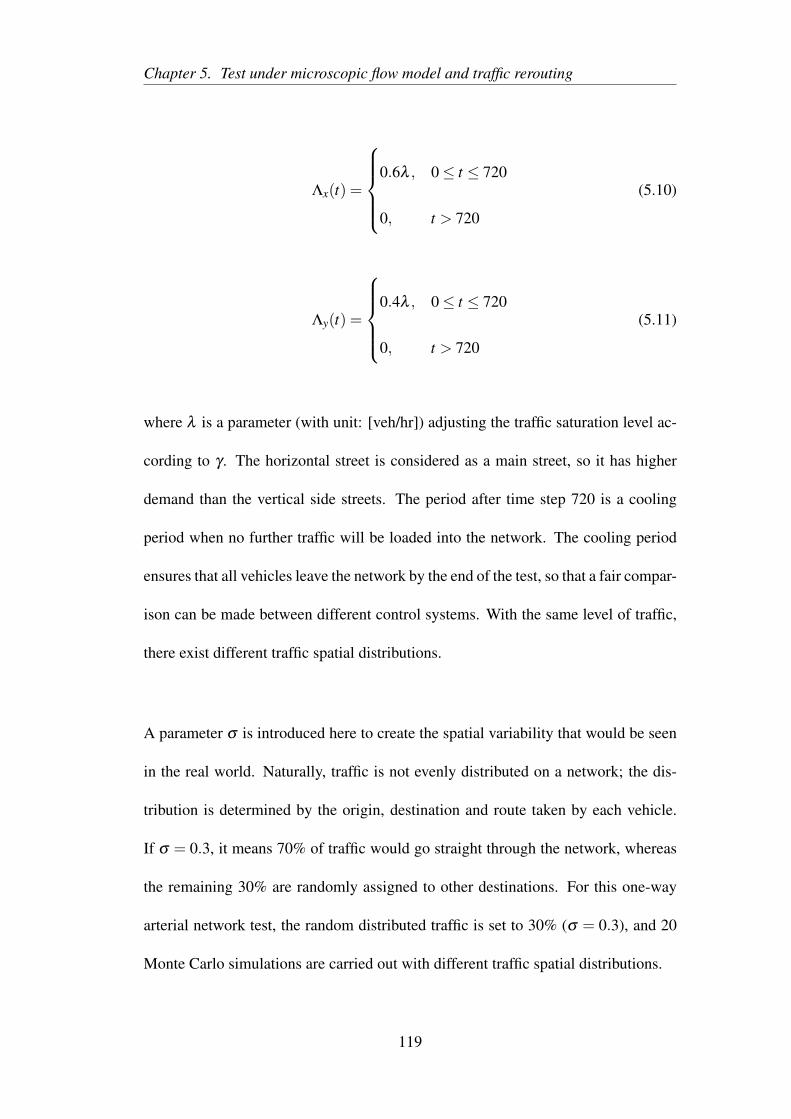
Chapter 5. Test under microscopic flow model and traffic rerouting
Λx(t) =
0.6λ , 0≤ t ≤ 720
0, t > 720
(5.10)
Λy(t) =
0.4λ , 0≤ t ≤ 720
0, t > 720
(5.11)
where λ is a parameter (with unit: [veh/hr]) adjusting the traffic saturation level ac-
cording to γ . The horizontal street is considered as a main street, so it has higher
demand than the vertical side streets. The period after time step 720 is a cooling
period when no further traffic will be loaded into the network. The cooling period
ensures that all vehicles leave the network by the end of the test, so that a fair compar-
ison can be made between different control systems. With the same level of traffic,
there exist different traffic spatial distributions.
A parameter σ is introduced here to create the spatial variability that would be seen
in the real world. Naturally, traffic is not evenly distributed on a network; the dis-
tribution is determined by the origin, destination and route taken by each vehicle.
If σ = 0.3, it means 70% of traffic would go straight through the network, whereas
the remaining 30% are randomly assigned to other destinations. For this one-way
arterial network test, the random distributed traffic is set to 30% (σ = 0.3), and 20
Monte Carlo simulations are carried out with different traffic spatial distributions.
119
Chapter 5. Test under microscopic flow model and traffic rerouting
5.3.2 Settings of the test control systems
In terms of the traffic control systems, there are some predefined settings for the
comparison test. The test chosen four control systems: TUC system (TUC), decen-
tralised TUC system (TUC_D), cyclic max-pressure controller (MP_C) and acyclic
max-pressure controller (MP). In previous Chapter 4, offset has been found as a
cause to create performance differences between centralised and decentralised sys-
tems. For fair comparison in this test, all the cyclic systems are using the same offset
control (Gazis offset controller). In this case, the difference between the systems are
mainly from the split control, so that the TUC system is a centralised control where
the other systems are decentralised. The Hybrid system mentioned in chapter 3 has
not been chosen to test on SUMO. The hybrid system only outperform the TUC sys-
tem when γ is low, otherwise, it has similar performance with the TUC (according
to the CTM test results in chapter 4). The TUC system derives centralised green
split, where cyclic and acyclic max-pressure derive decentralised green split. The
decentralised TUC system is a modified TUC system using as a reference in the test.
The green splits of the decentralised TUC are derived separately for each node, so
that the decentralised TUC has individual L matrices for each node. The original
TUC only has a single L matrix for the entire network (see Section 3.3.1). TUC,
decentralised TUC and cyclic max-pressure controller are cyclic control, and their
signal timing plans consist of cycle time, offset and green split. The three cyclic
control systems are using the same decentralised offset controller for comparison
purpose, hence, the cycle time used for each node is the same as well. The cycle
time was examined over different traffic saturation levels and control systems on the
120
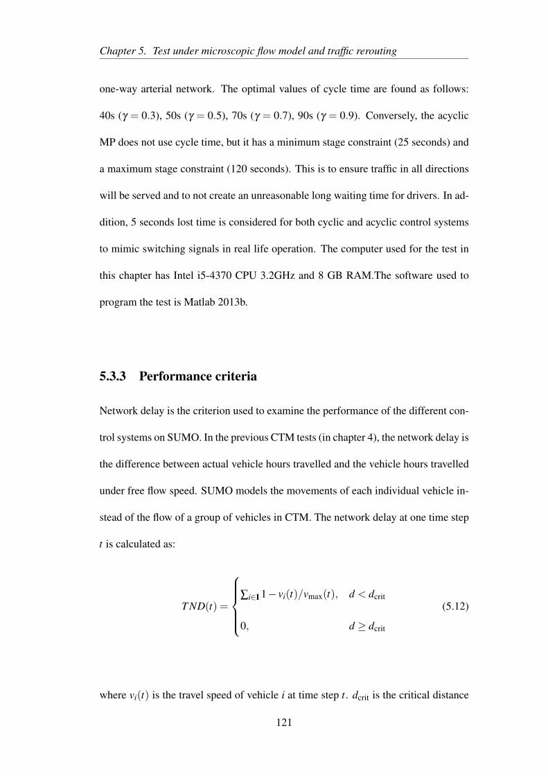
Chapter 5. Test under microscopic flow model and traffic rerouting
one-way arterial network. The optimal values of cycle time are found as follows:
40s (γ = 0.3), 50s (γ = 0.5), 70s (γ = 0.7), 90s (γ = 0.9). Conversely, the acyclic
MP does not use cycle time, but it has a minimum stage constraint (25 seconds) and
a maximum stage constraint (120 seconds). This is to ensure traffic in all directions
will be served and to not create an unreasonable long waiting time for drivers. In ad-
dition, 5 seconds lost time is considered for both cyclic and acyclic control systems
to mimic switching signals in real life operation. The computer used for the test in
this chapter has Intel i5-4370 CPU 3.2GHz and 8 GB RAM.The software used to
program the test is Matlab 2013b.
5.3.3 Performance criteria
Network delay is the criterion used to examine the performance of the different con-
trol systems on SUMO. In the previous CTM tests (in chapter 4), the network delay is
the difference between actual vehicle hours travelled and the vehicle hours travelled
under free flow speed. SUMO models the movements of each individual vehicle in-
stead of the flow of a group of vehicles in CTM. The network delay at one time step
t is calculated as:
T ND(t) =
∑i∈I 1− vi(t)/vmax(t), d < dcrit
0, d ≥ dcrit
(5.12)
where vi(t) is the travel speed of vehicle i at time step t. dcrit is the critical distance
121
Chapter 5. Test under microscopic flow model and traffic rerouting
between two continuous vehicles, and its value is converted from the critical density
ρcrit used in CTM.
Bandwidth is another criteria to see how traffic control systems are performed. Effi-
cient coordination between signal controllers can help a platoon of vehicles to travel
through them without stopping. The movement of this platoon of vehicles under a
time-space diagram will be visualised as a pair of speed lines (see Figure 5.9), the
band formed by these two speed lines is called green band. The width of the green
band is bandwidth, and it indicates the portion of a time period over a signal cycle
that the traffic can travel within the green band. When calculating the bandwidth of a
route, the signal plans of controllers along the route are compared against the speed
lines (see Figure 5.9). The speed lines can also be understood as vehicles' trajectory
under free flow speed. However, the part of a bandwidth is excluded when there
exists residual queues along the route.
122
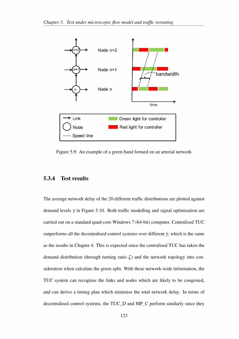
Chapter 5. Test under microscopic flow model and traffic rerouting
Figure 5.9: An example of a green band formed on an arterial network
5.3.4 Test results
The average network delay of the 20 different traffic distributions are plotted against
demand levels γ in Figure 5.10. Both traffic modelling and signal optimisation are
carried out on a standard quad-core Windows 7 (64-bit) computer. Centralised TUC
outperforms all the decentralised control systems over different γ , which is the same
as the results in Chapter 4. This is expected since the centralised TUC has taken the
demand distribution (through turning ratio ζ ) and the network topology into con-
sideration when calculate the green split. With these network-wide information, the
TUC system can recognise the links and nodes which are likely to be congested,
and can derive a timing plan which minimise the total network delay. In terms of
decentralised control systems, the TUC_D and MP_C perform similarly since they
123
Chapter 5. Test under microscopic flow model and traffic rerouting
both are queue-based control systems and use the same external offset controller.
The perfromances of the two control systems can differ in a spill over scenario, how-
ever, this one-dimensional network has not observed a significant spill over in traffic
queues. The acyclic MP performs the worst in the decentralised systems. According
to [8] and [6], MP has been proved that can stabilise the queue length when demand
is in a feasible range. Meanwhile, the MP control is not designed for minimising the
network delay.
In this one-way arterial network, the average bandwidth of the horizontal main street
is calculated and the results are in Figure 5.11. The centralised TUC creates widest
bandwidth on the main street. This is not only an intuitive observation, but the TUC
's centralised green split did helped the offset control in previous study [107]. When
calculating the green split, TUC priorities the routes which have more traffic and
allocates longer green split. With the longer green split on a route, it will form a
wider bandwidth. The bandwidth created by the TUC_D and cyclic MP are similar.
Both TUC_D and MP_C are operated under the same offset controller and cyclic
feature. Comparing to the cyclic systems, the acyclic MP has the narrowest band-
width. Different from the control systems which tended to group vehicles together
and maximise traffic flow, acyclic MP aims to stabilise the queue distribution instead
of minimise the network delay. The narrow bandwidth formed in acyclic MP also
explained why it is not performed well on the network delay.
124
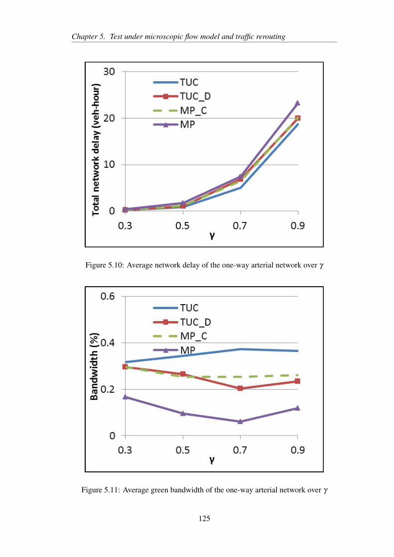
Chapter 5. Test under microscopic flow model and traffic rerouting
Figure 5.10: Average network delay of the one-way arterial network over γ
Figure 5.11: Average green bandwidth of the one-way arterial network over γ
125
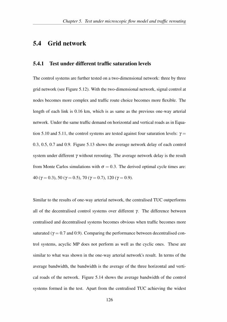
Chapter 5. Test under microscopic flow model and traffic rerouting
5.4 Grid network
5.4.1 Test under different traffic saturation levels
The control systems are further tested on a two-dimensional network: three by three
grid network (see Figure 5.12). With the two-dimensional network, signal control at
nodes becomes more complex and traffic route choice becomes more flexible. The
length of each link is 0.16 km, which is as same as the previous one-way arterial
network. Under the same traffic demand on horizontal and vertical roads as in Equa-
tion 5.10 and 5.11, the control systems are tested against four saturation levels: γ =
0.3, 0.5, 0.7 and 0.9. Figure 5.13 shows the average network delay of each control
system under different γ without rerouting. The average network delay is the result
from Monte Carlos simulations with σ = 0.3. The derived optimal cycle times are:
40 (γ = 0.3), 50 (γ = 0.5), 70 (γ = 0.7), 120 (γ = 0.9).
Similar to the results of one-way arterial network, the centralised TUC outperforms
all of the decentralised control systems over different γ . The difference between
centralised and decentralised systems becomes obvious when traffic becomes more
saturated (γ = 0.7 and 0.9). Comparing the performance between decentralised con-
trol systems, acyclic MP does not perform as well as the cyclic ones. These are
similar to what was shown in the one-way arterial network's result. In terms of the
average bandwidth, the bandwidth is the average of the three horizontal and verti-
cal roads of the network. Figure 5.14 shows the average bandwidth of the control
systems formed in the test. Apart from the centralised TUC achieving the widest
126
Chapter 5. Test under microscopic flow model and traffic rerouting
bandwidth, the bandwidth formed in all cyclic control systems reached 30% when
network is fully saturated (γ = 0.9). In this case, the performance difference between
centralised and decentralised control systems is not clear to see from the average
bandwidth. Figure 5.15 is further plotted to show the average queue length formed
at each node when γ = 0.9 over the test period. The centralised TUC has less of a
queue at node 1 and 4, but a longer queue at node 2 and 3. This means centralised
TUC allowed more traffic to travel through the node 1 to its downstream compared
to the decentralised systems. The nodes 1,4,7 are the boundary nodes, where traffic
flows into the network. Controlling traffic properly at those boundary nodes directly
affects how the downstream nodes perform. So the performance difference between
centralised and decentralised control systems is due to the same reason as in the one-
dimensional network test. The centralised control can minimise the entire network
delay, when it holds accurate traffic information through the network.
In order to capture drivers' response to the real-time traffic condition, a dynamic
rerouting algorithm (see Section 5.2.2) is implemented on the three by three grid
network. Figure 5.16 is the network delay of different control systems over γ where
rerouting is allowed. The results are the average of 20 Monte Carlo simulations
when σ = 0.3. The traffic saturation levels and distributions are the same as the test
without rerouting. All decentralised control systems have significant reduction in
network delays, but not the centralised TUC. The centralised TUC has predefined
settings (L matrix and nominal green split gN). They prioritise some more con-
gested routes and remain unchanged through the test. This could be one reason that
127
Chapter 5. Test under microscopic flow model and traffic rerouting
the centralised TUC has not improved much after rerouting. Decentralised systems
can not prioritise any routes but only links at each node. Therefore, they are more
adaptive to the changes in traffic distribution caused by rerouting. Comparing the
decentralised systems, acyclic MP has the highest improvement in delay. It outper-
forms the centralised TUC at γ = 0.5 and 0.7. Decentralised TUC and cyclic MP
are slightly worse than centralised TUC in performance, but both are more efficient
than the case without rerouting. Figure 5.17 is the average bandwidth measured
from the three horizontal roads and vertical roads. The centralised TUC still has the
widest bandwidth and acyclic MP has the narrowest. However, acyclic MP's band-
width slightly increased compared to the result without rerouting. The average queue
length of each control system is plotted in Figure 5.18 for γ = 0.9. Clearly, the de-
centralised control system reduced queue at boundary nodes, where the centralised
control system has a similar queue length as before. The rerouting results here show
that there can be a great impact on the performance of decentralised control system
by allowing traffic to reroute.
128
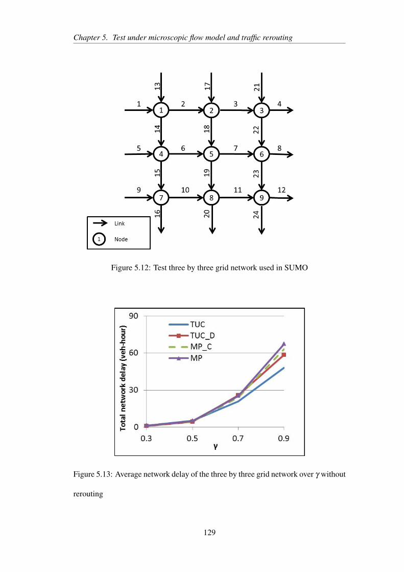
Chapter 5. Test under microscopic flow model and traffic rerouting
Figure 5.12: Test three by three grid network used in SUMO
Figure 5.13: Average network delay of the three by three grid network over γ without
rerouting
129
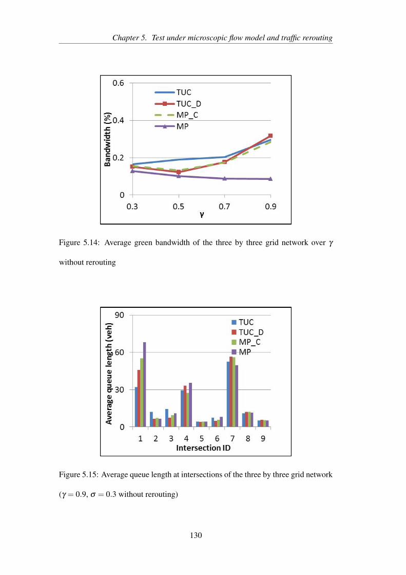
Chapter 5. Test under microscopic flow model and traffic rerouting
Figure 5.14: Average green bandwidth of the three by three grid network over γ
without rerouting
Figure 5.15: Average queue length at intersections of the three by three grid network
(γ = 0.9, σ = 0.3 without rerouting)
130
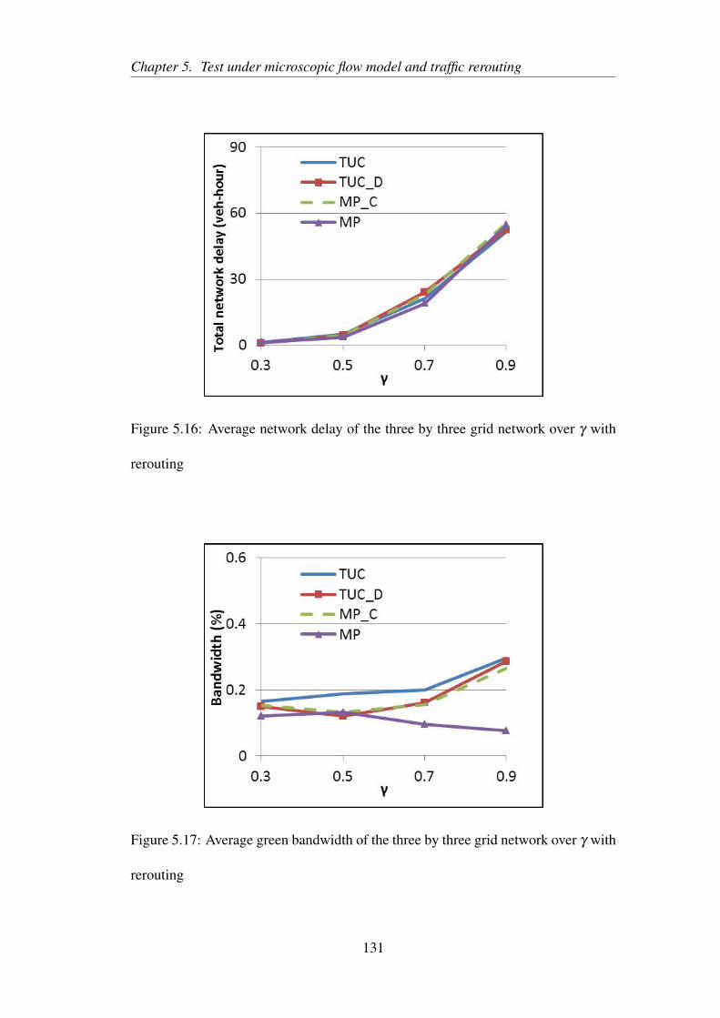
Chapter 5. Test under microscopic flow model and traffic rerouting
Figure 5.16: Average network delay of the three by three grid network over γ with
rerouting
Figure 5.17: Average green bandwidth of the three by three grid network over γ with
rerouting
131
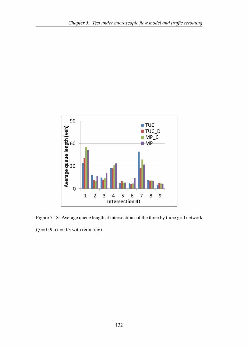
Chapter 5. Test under microscopic flow model and traffic rerouting
Figure 5.18: Average queue length at intersections of the three by three grid network
(γ = 0.9, σ = 0.3 with rerouting)
132
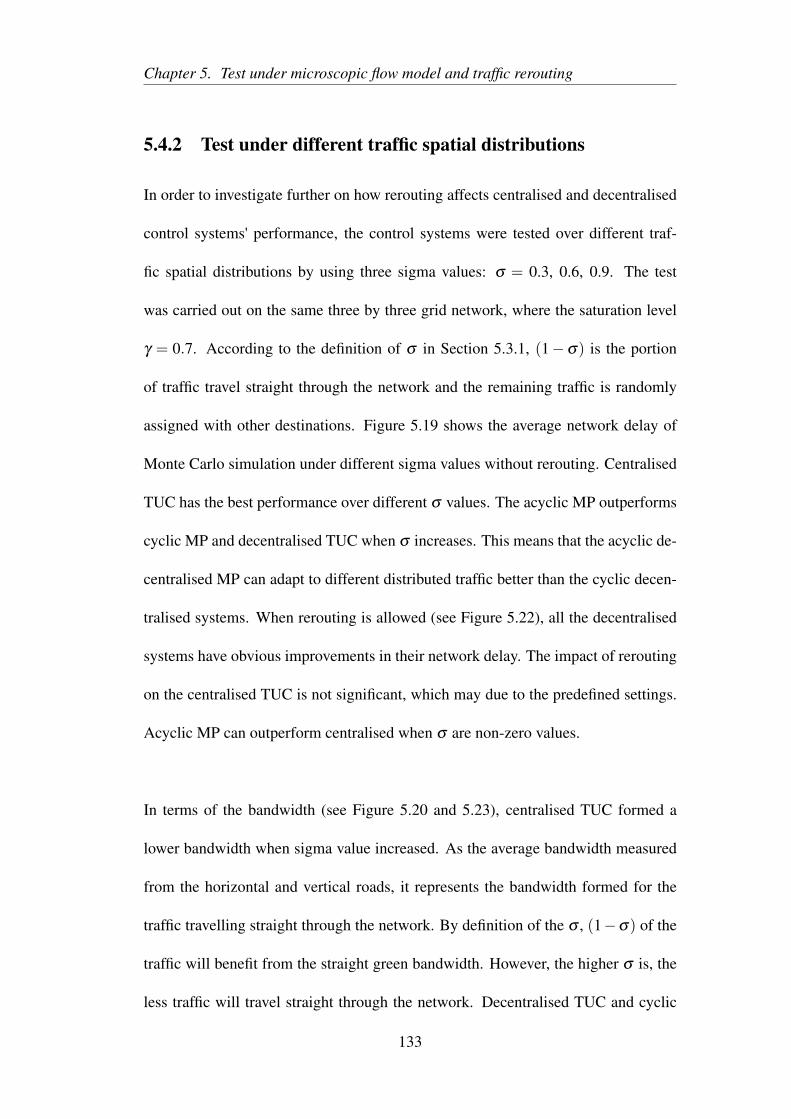
Chapter 5. Test under microscopic flow model and traffic rerouting
5.4.2 Test under different traffic spatial distributions
In order to investigate further on how rerouting affects centralised and decentralised
control systems' performance, the control systems were tested over different traf-
fic spatial distributions by using three sigma values: σ = 0.3, 0.6, 0.9. The test
was carried out on the same three by three grid network, where the saturation level
γ = 0.7. According to the definition of σ in Section 5.3.1, (1−σ) is the portion
of traffic travel straight through the network and the remaining traffic is randomly
assigned with other destinations. Figure 5.19 shows the average network delay of
Monte Carlo simulation under different sigma values without rerouting. Centralised
TUC has the best performance over different σ values. The acyclic MP outperforms
cyclic MP and decentralised TUC when σ increases. This means that the acyclic de-
centralised MP can adapt to different distributed traffic better than the cyclic decen-
tralised systems. When rerouting is allowed (see Figure 5.22), all the decentralised
systems have obvious improvements in their network delay. The impact of rerouting
on the centralised TUC is not significant, which may due to the predefined settings.
Acyclic MP can outperform centralised when σ are non-zero values.
In terms of the bandwidth (see Figure 5.20 and 5.23), centralised TUC formed a
lower bandwidth when sigma value increased. As the average bandwidth measured
from the horizontal and vertical roads, it represents the bandwidth formed for the
traffic travelling straight through the network. By definition of the σ , (1−σ) of the
traffic will benefit from the straight green bandwidth. However, the higher σ is, the
less traffic will travel straight through the network. Decentralised TUC and cyclic
133
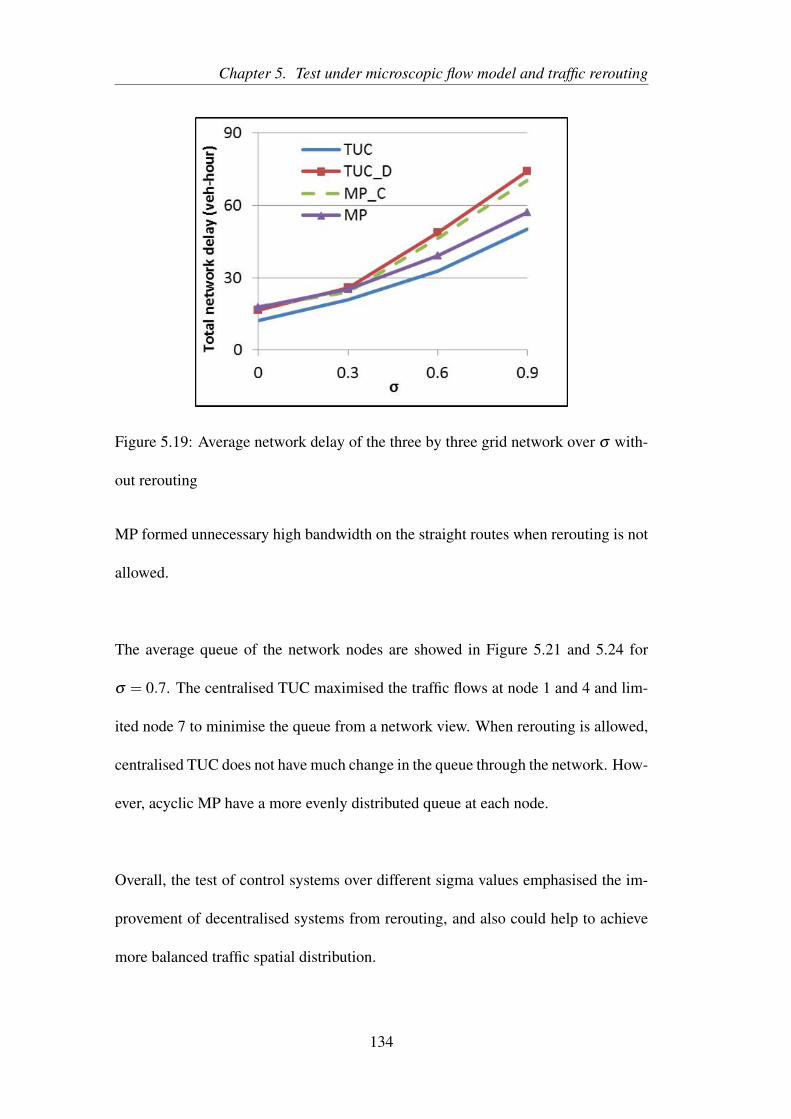
Chapter 5. Test under microscopic flow model and traffic rerouting
Figure 5.19: Average network delay of the three by three grid network over σ with-
out rerouting
MP formed unnecessary high bandwidth on the straight routes when rerouting is not
allowed.
The average queue of the network nodes are showed in Figure 5.21 and 5.24 for
σ = 0.7. The centralised TUC maximised the traffic flows at node 1 and 4 and lim-
ited node 7 to minimise the queue from a network view. When rerouting is allowed,
centralised TUC does not have much change in the queue through the network. How-
ever, acyclic MP have a more evenly distributed queue at each node.
Overall, the test of control systems over different sigma values emphasised the im-
provement of decentralised systems from rerouting, and also could help to achieve
more balanced traffic spatial distribution.
134
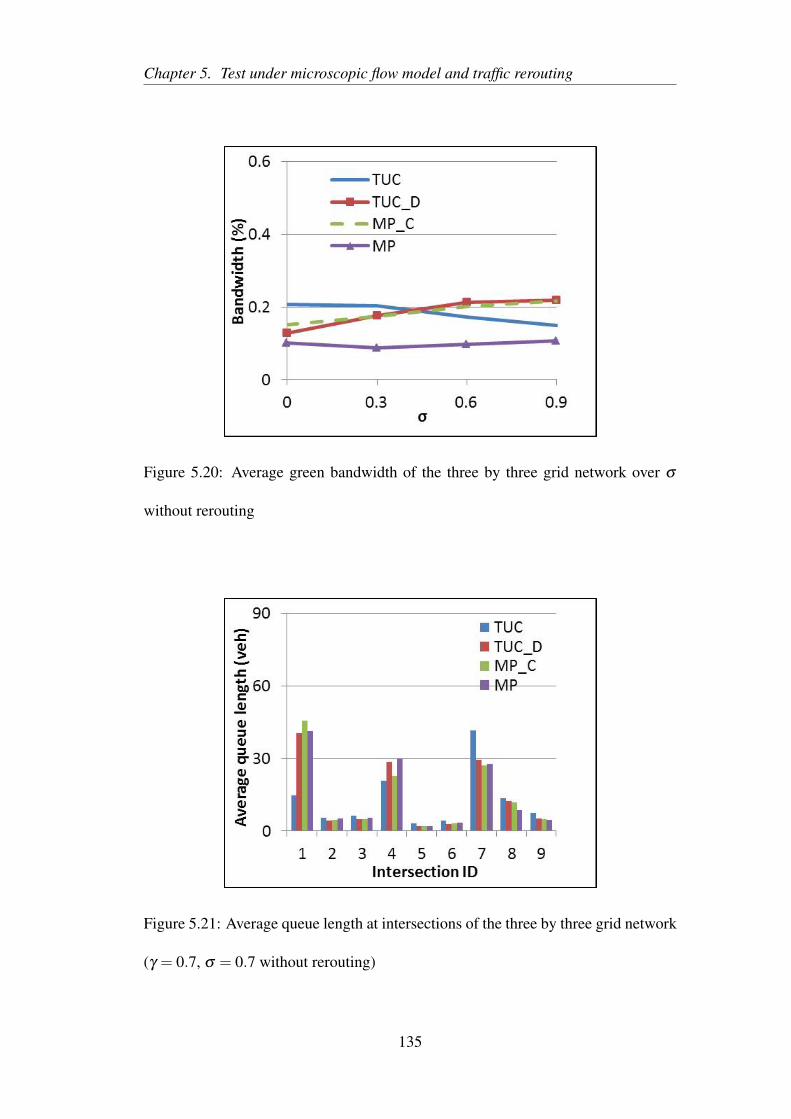
Chapter 5. Test under microscopic flow model and traffic rerouting
Figure 5.20: Average green bandwidth of the three by three grid network over σ
without rerouting
Figure 5.21: Average queue length at intersections of the three by three grid network
(γ = 0.7, σ = 0.7 without rerouting)
135
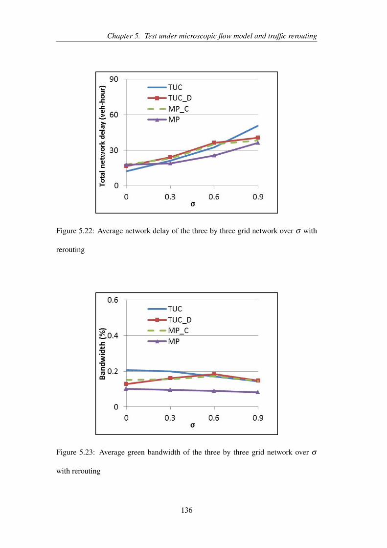
Chapter 5. Test under microscopic flow model and traffic rerouting
Figure 5.22: Average network delay of the three by three grid network over σ with
rerouting
Figure 5.23: Average green bandwidth of the three by three grid network over σ
with rerouting
136
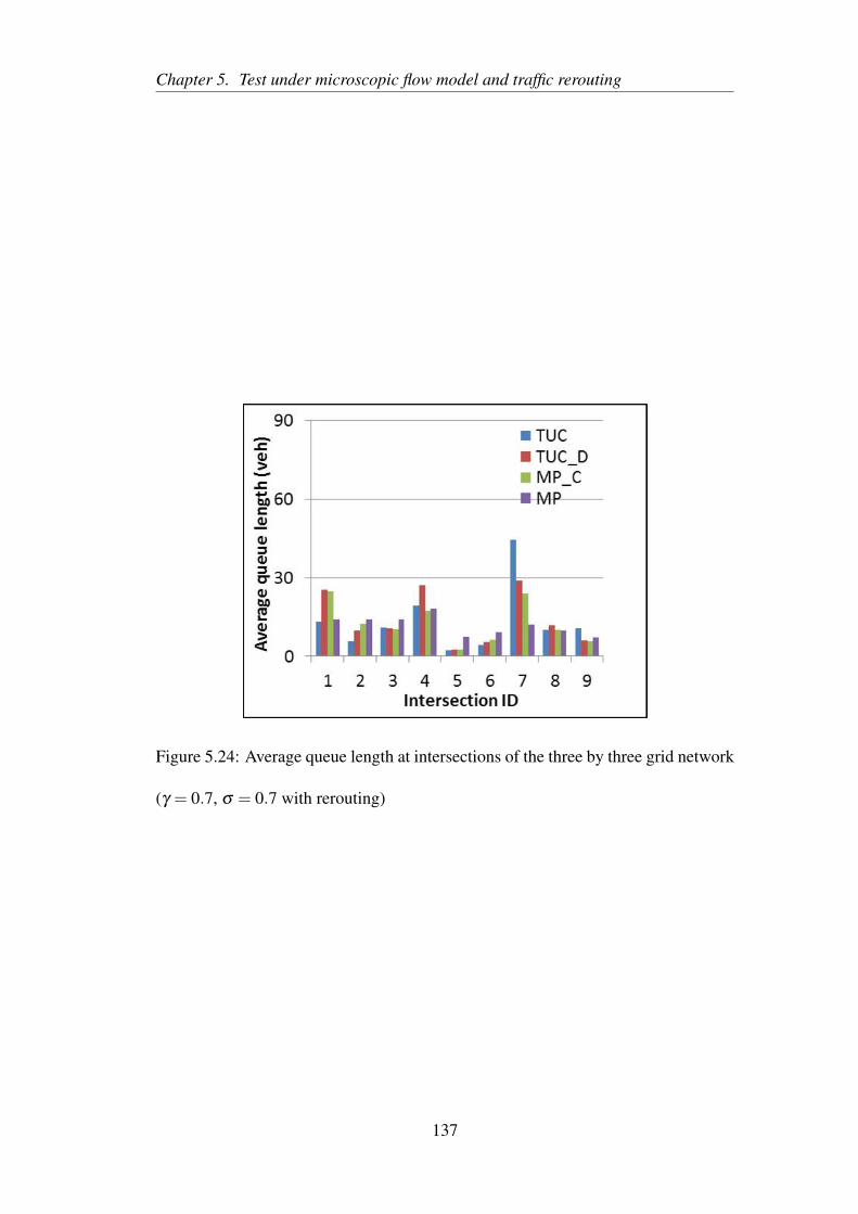
Chapter 5. Test under microscopic flow model and traffic rerouting
Figure 5.24: Average queue length at intersections of the three by three grid network
(γ = 0.7, σ = 0.7 with rerouting)
137
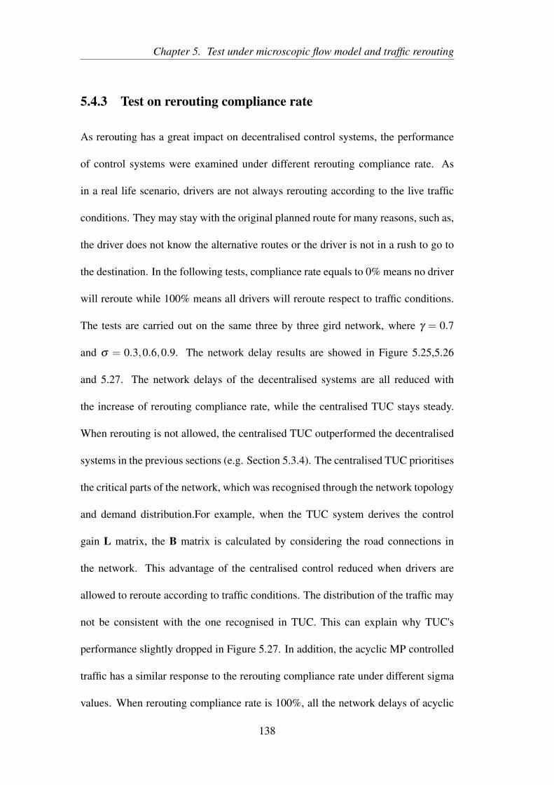
Chapter 5. Test under microscopic flow model and traffic rerouting
5.4.3 Test on rerouting compliance rate
As rerouting has a great impact on decentralised control systems, the performance
of control systems were examined under different rerouting compliance rate. As
in a real life scenario, drivers are not always rerouting according to the live traffic
conditions. They may stay with the original planned route for many reasons, such as,
the driver does not know the alternative routes or the driver is not in a rush to go to
the destination. In the following tests, compliance rate equals to 0% means no driver
will reroute while 100% means all drivers will reroute respect to traffic conditions.
The tests are carried out on the same three by three gird network, where γ = 0.7
and σ = 0.3,0.6,0.9. The network delay results are showed in Figure 5.25,5.26
and 5.27. The network delays of the decentralised systems are all reduced with
the increase of rerouting compliance rate, while the centralised TUC stays steady.
When rerouting is not allowed, the centralised TUC outperformed the decentralised
systems in the previous sections (e.g. Section 5.3.4). The centralised TUC prioritises
the critical parts of the network, which was recognised through the network topology
and demand distribution.For example, when the TUC system derives the control
gain L matrix, the B matrix is calculated by considering the road connections in
the network. This advantage of the centralised control reduced when drivers are
allowed to reroute according to traffic conditions. The distribution of the traffic may
not be consistent with the one recognised in TUC. This can explain why TUC's
performance slightly dropped in Figure 5.27. In addition, the acyclic MP controlled
traffic has a similar response to the rerouting compliance rate under different sigma
values. When rerouting compliance rate is 100%, all the network delays of acyclic
138
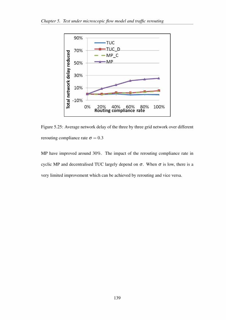
Chapter 5. Test under microscopic flow model and traffic rerouting
Figure 5.25: Average network delay of the three by three grid network over different
rerouting compliance rate σ = 0.3
MP have improved around 30%. The impact of the rerouting compliance rate in
cyclic MP and decentralised TUC largely depend on σ . When σ is low, there is a
very limited improvement which can be achieved by rerouting and vice versa.
139
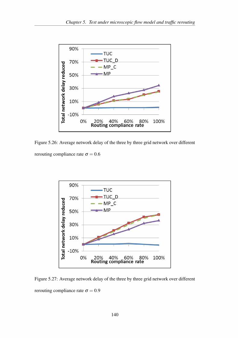
Chapter 5. Test under microscopic flow model and traffic rerouting
Figure 5.26: Average network delay of the three by three grid network over different
rerouting compliance rate σ = 0.6
Figure 5.27: Average network delay of the three by three grid network over different
rerouting compliance rate σ = 0.9
140
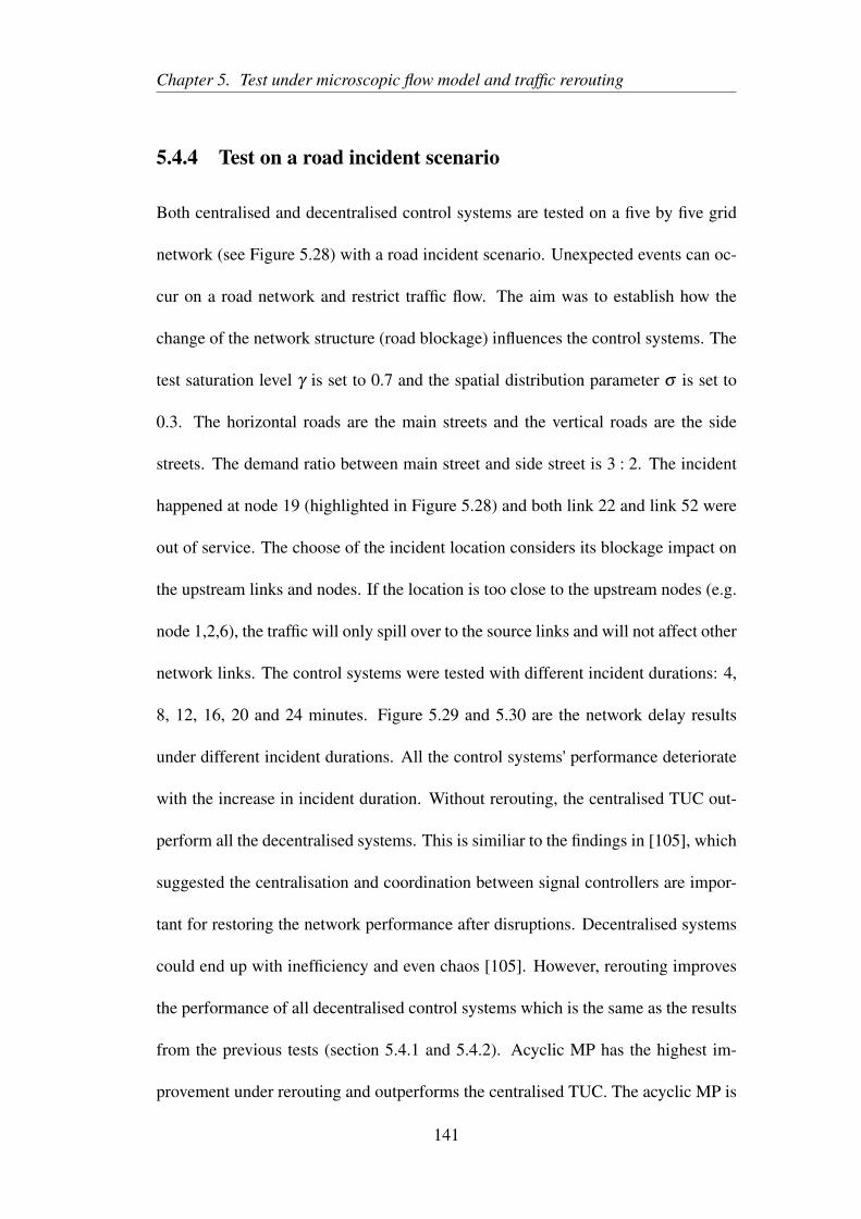
Chapter 5. Test under microscopic flow model and traffic rerouting
5.4.4 Test on a road incident scenario
Both centralised and decentralised control systems are tested on a five by five grid
network (see Figure 5.28) with a road incident scenario. Unexpected events can oc-
cur on a road network and restrict traffic flow. The aim was to establish how the
change of the network structure (road blockage) influences the control systems. The
test saturation level γ is set to 0.7 and the spatial distribution parameter σ is set to
0.3. The horizontal roads are the main streets and the vertical roads are the side
streets. The demand ratio between main street and side street is 3 : 2. The incident
happened at node 19 (highlighted in Figure 5.28) and both link 22 and link 52 were
out of service. The choose of the incident location considers its blockage impact on
the upstream links and nodes. If the location is too close to the upstream nodes (e.g.
node 1,2,6), the traffic will only spill over to the source links and will not affect other
network links. The control systems were tested with different incident durations: 4,
8, 12, 16, 20 and 24 minutes. Figure 5.29 and 5.30 are the network delay results
under different incident durations. All the control systems' performance deteriorate
with the increase in incident duration. Without rerouting, the centralised TUC out-
perform all the decentralised systems. This is similiar to the findings in [105], which
suggested the centralisation and coordination between signal controllers are impor-
tant for restoring the network performance after disruptions. Decentralised systems
could end up with inefficiency and even chaos [105]. However, rerouting improves
the performance of all decentralised control systems which is the same as the results
from the previous tests (section 5.4.1 and 5.4.2). Acyclic MP has the highest im-
provement under rerouting and outperforms the centralised TUC. The acyclic MP is
141
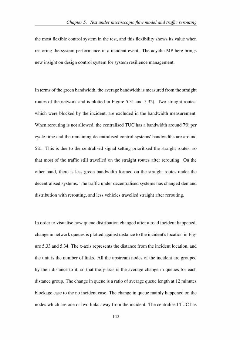
Chapter 5. Test under microscopic flow model and traffic rerouting
the most flexible control system in the test, and this flexibility shows its value when
restoring the system performance in a incident event. The acyclic MP here brings
new insight on design control system for system resilience management.
In terms of the green bandwidth, the average bandwidth is measured from the straight
routes of the network and is plotted in Figure 5.31 and 5.32). Two straight routes,
which were blocked by the incident, are excluded in the bandwidth measurement.
When rerouting is not allowed, the centralised TUC has a bandwidth around 7% per
cycle time and the remaining decentralised control systems' bandwidths are around
5%. This is due to the centralised signal setting prioritised the straight routes, so
that most of the traffic still travelled on the straight routes after rerouting. On the
other hand, there is less green bandwidth formed on the straight routes under the
decentralised systems. The traffic under decentralised systems has changed demand
distribution with rerouting, and less vehicles travelled straight after rerouting.
In order to visualise how queue distribution changed after a road incident happened,
change in network queues is plotted against distance to the incident's location in Fig-
ure 5.33 and 5.34. The x-axis represents the distance from the incident location, and
the unit is the number of links. All the upstream nodes of the incident are grouped
by their distance to it, so that the y-axis is the average change in queues for each
distance group. The change in queue is a ratio of average queue length at 12 minutes
blockage case to the no incident case. The change in queue mainly happened on the
nodes which are one or two links away from the incident. The centralised TUC has
142
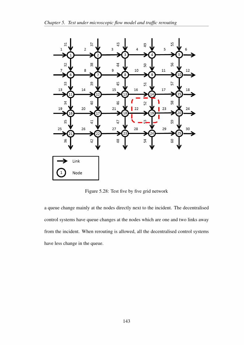
Chapter 5. Test under microscopic flow model and traffic rerouting
Figure 5.28: Test five by five grid network
a queue change mainly at the nodes directly next to the incident. The decentralised
control systems have queue changes at the nodes which are one and two links away
from the incident. When rerouting is allowed, all the decentralised control systems
have less change in the queue.
143
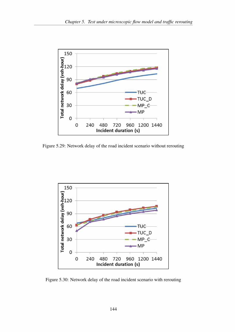
Chapter 5. Test under microscopic flow model and traffic rerouting
Figure 5.29: Network delay of the road incident scenario without rerouting
Figure 5.30: Network delay of the road incident scenario with rerouting
144
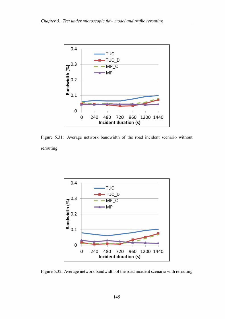
Chapter 5. Test under microscopic flow model and traffic rerouting
Figure 5.31: Average network bandwidth of the road incident scenario without
rerouting
Figure 5.32: Average network bandwidth of the road incident scenario with rerouting
145
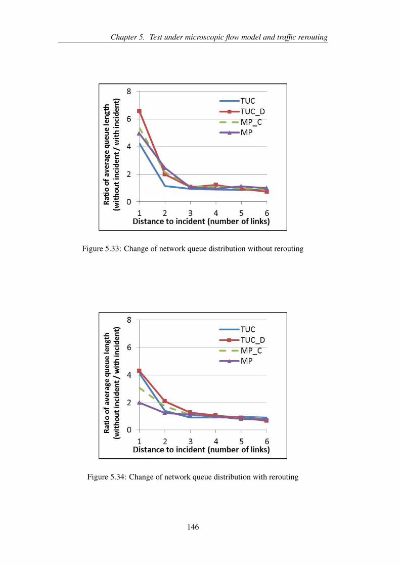
Chapter 5. Test under microscopic flow model and traffic rerouting
Figure 5.33: Change of network queue distribution without rerouting
Figure 5.34: Change of network queue distribution with rerouting
146
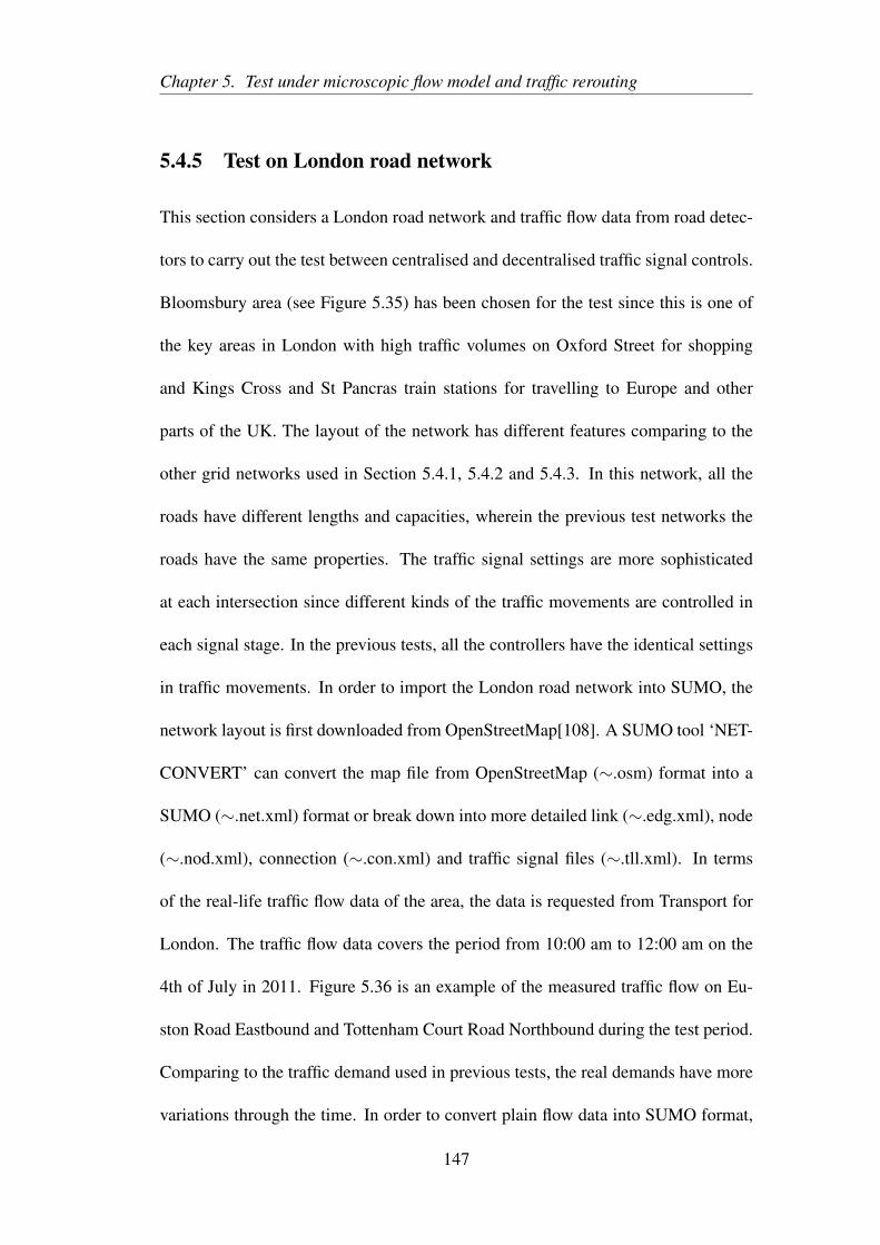
Chapter 5. Test under microscopic flow model and traffic rerouting
5.4.5 Test on London road network
This section considers a London road network and traffic flow data from road detec-
tors to carry out the test between centralised and decentralised traffic signal controls.
Bloomsbury area (see Figure 5.35) has been chosen for the test since this is one of
the key areas in London with high traffic volumes on Oxford Street for shopping
and Kings Cross and St Pancras train stations for travelling to Europe and other
parts of the UK. The layout of the network has different features comparing to the
other grid networks used in Section 5.4.1, 5.4.2 and 5.4.3. In this network, all the
roads have different lengths and capacities, wherein the previous test networks the
roads have the same properties. The traffic signal settings are more sophisticated
at each intersection since different kinds of the traffic movements are controlled in
each signal stage. In the previous tests, all the controllers have the identical settings
in traffic movements. In order to import the London road network into SUMO, the
network layout is first downloaded from OpenStreetMap[108]. A SUMO tool ‘NET-
CONVERT’ can convert the map file from OpenStreetMap (∼.osm) format into a
SUMO (∼.net.xml) format or break down into more detailed link (∼.edg.xml), node
(∼.nod.xml), connection (∼.con.xml) and traffic signal files (∼.tll.xml). In terms
of the real-life traffic flow data of the area, the data is requested from Transport for
London. The traffic flow data covers the period from 10:00 am to 12:00 am on the
4th of July in 2011. Figure 5.36 is an example of the measured traffic flow on Eu-
ston Road Eastbound and Tottenham Court Road Northbound during the test period.
Comparing to the traffic demand used in previous tests, the real demands have more
variations through the time. In order to convert plain flow data into SUMO format,
147
Chapter 5. Test under microscopic flow model and traffic rerouting
a SUMO tool ‘DFROUTER’ can allow a user to compute vehicles’ routes from road
detector counts. Once the routes are computed, a SUMO tool ‘DUAROUTER’ can
convert them into a route file (∼.rou.xml). The route file in SUMO defines the traffic
demand, which has a trip starting time, a route to travel and driver’s characters for
each individual vehicle.
The test settings are the same with the previous grid network tests, where four signal
controllers (TUC, cyclic Max-pressure (MP_C) and non-cyclic Max-pressure (MP))
are compared in network delay with rerouting. Figure 5.37 shows the network per-
formance results between different controllers. Due to the centralised feature, TUC
has the advantage over the other decentralised controls when no rerouting is allowed.
The TUC_D and MP_C have similar performance, and it is interesting to see non-
cyclic MP performed better than the two cyclic one. This is due to the non-cyclic
MP do not have a fixed sequence of green lights given to different traffic movements,
and it is more flexible to prioritise the direction with long queues. After rerouting
is allowed, it is not surprising that all controller have improvements in their perfor-
mances. The reason for this improvement is because the minor roads in this London
Bloomsbury network create more alternative routes inside the network. Overall, the
majority of the test results are consistent with the founding in the previous tests.
148
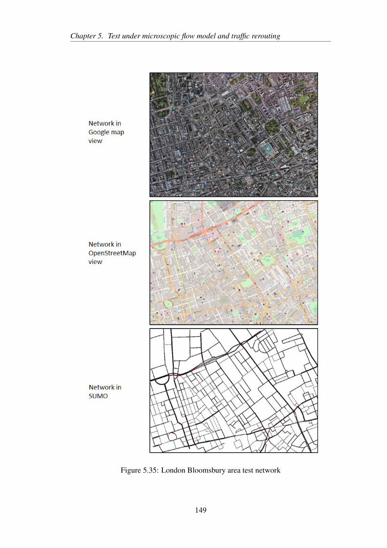
Chapter 5. Test under microscopic flow model and traffic rerouting
Figure 5.35: London Bloomsbury area test network
149
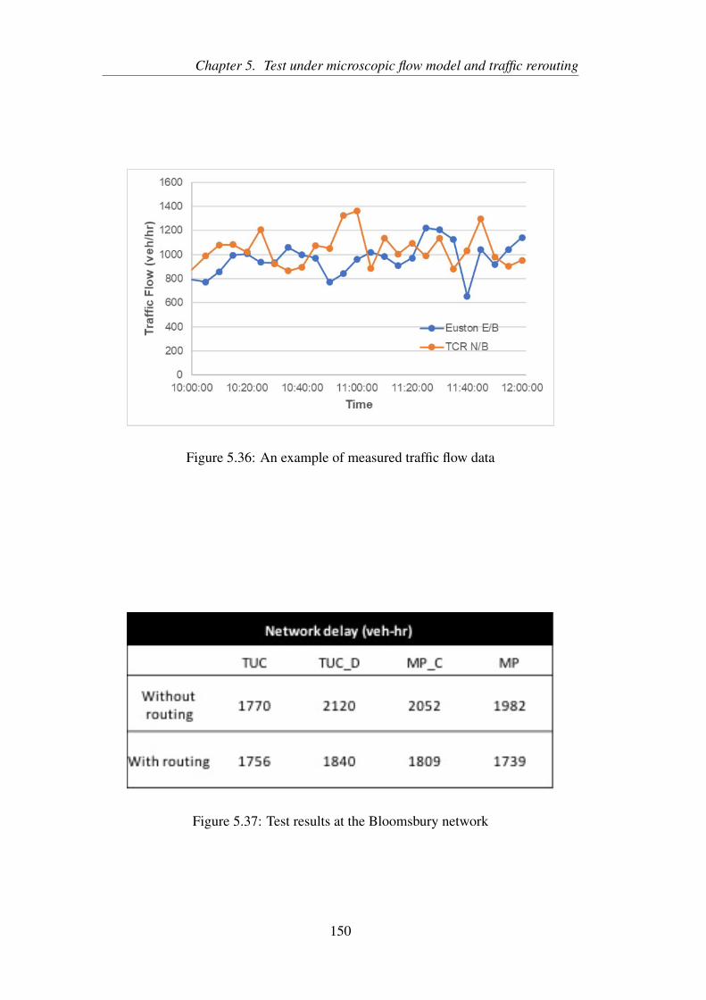
Chapter 5. Test under microscopic flow model and traffic rerouting
Figure 5.36: An example of measured traffic flow data
Figure 5.37: Test results at the Bloomsbury network
150
Chapter 5. Test under microscopic flow model and traffic rerouting
5.4.6 An adaptive TUC system with rerouting control
A new centralised control system is proposed here to test against conventional cen-
tralised TUC and decentralised TUC systems. The three TUC systems are tested
under different demand levels and distributions on a three by three grid network
(see Figure 5.12). In previous tests, centralised TUC was able to outperform de-
centralised control systems since it considered network topology and demand dis-
tribution. However, the decentralised systems received significant improvement in
performance when drivers were allowed to reroute respect to traffic conditions. An
adaptive centralised system is proposed here to see if the centralised system can also
improve its performance by allowing drivers to reroute. The new adaptive centralised
control collects real-time demand distribution (through turning ratio ζ ) on the test
network every signal cycle. The demand distribution will be used to recalculate the
control gain matrix L of TUC system.
When testing under different demand levels, demand level parameter γ is set to be
0.3,0.5,0.7,0.9 and the distribution parameter σ is fixed to 0.3. The network delay
result without rerouting is in Figure 5.38, where the two centralised TUC outperform
the decentralised TUC under through all demand levels. The adaptive TUC perform
slightly better than the conventional TUC. This is due to the signal setting (L ma-
trix) in conventional TUC is derived from the average demand distribution through
the entire test period, where the adaptive TUC uses a shorter time interval and update
the distribution in real-time. When rerouting is allowed (see Figure 5.39 and 5.40),
both decentralised TUC and adaptive centralised TUC have improved in network de-
151
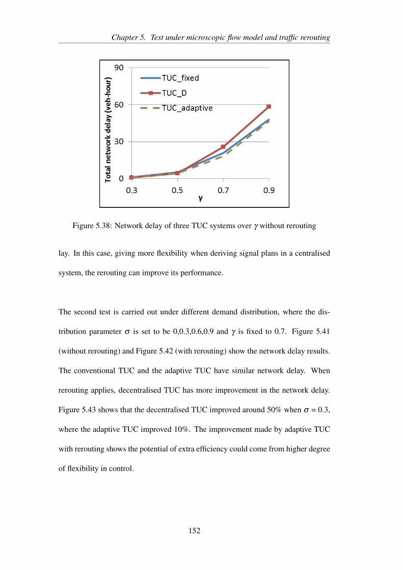
Chapter 5. Test under microscopic flow model and traffic rerouting
Figure 5.38: Network delay of three TUC systems over γ without rerouting
lay. In this case, giving more flexibility when deriving signal plans in a centralised
system, the rerouting can improve its performance.
The second test is carried out under different demand distribution, where the dis-
tribution parameter σ is set to be 0,0.3,0.6,0.9 and γ is fixed to 0.7. Figure 5.41
(without rerouting) and Figure 5.42 (with rerouting) show the network delay results.
The conventional TUC and the adaptive TUC have similar network delay. When
rerouting applies, decentralised TUC has more improvement in the network delay.
Figure 5.43 shows that the decentralised TUC improved around 50% when σ = 0.3,
where the adaptive TUC improved 10%. The improvement made by adaptive TUC
with rerouting shows the potential of extra efficiency could come from higher degree
of flexibility in control.
152
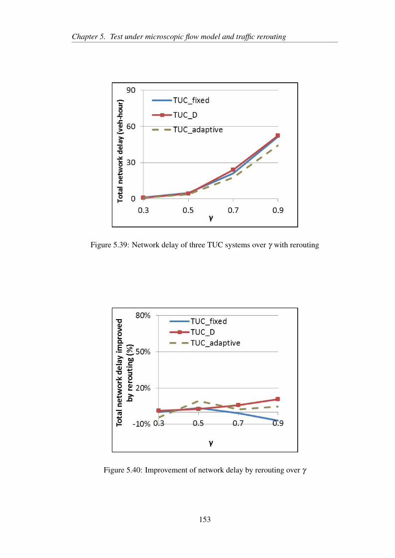
Chapter 5. Test under microscopic flow model and traffic rerouting
Figure 5.39: Network delay of three TUC systems over γ with rerouting
Figure 5.40: Improvement of network delay by rerouting over γ
153
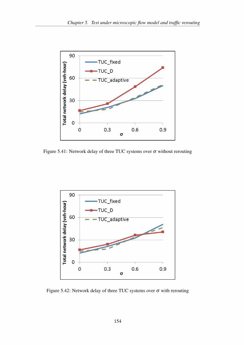
Chapter 5. Test under microscopic flow model and traffic rerouting
Figure 5.41: Network delay of three TUC systems over σ without rerouting
Figure 5.42: Network delay of three TUC systems over σ with rerouting
154
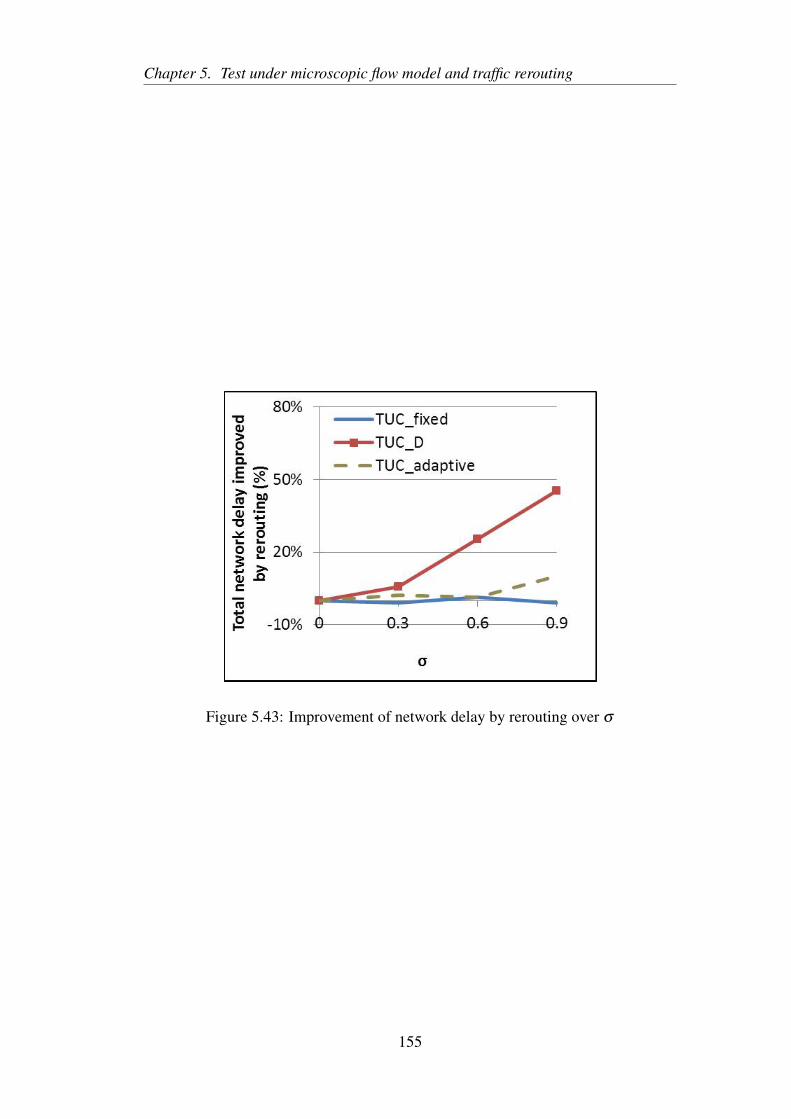
Chapter 5. Test under microscopic flow model and traffic rerouting
Figure 5.43: Improvement of network delay by rerouting over σ
155
Chapter 5. Test under microscopic flow model and traffic rerouting
5.5 Summary
This chapter compared the performance between centralised and decentralised con-
trol systems on a microscopic flow model at SUMO. The control systems are tested
under different traffic saturation levels and distributions first, and a dynamic rerout-
ing algorithm is implemented to allow traffic rerouting according to the traffic con-
ditions. The results show the improvement in decentralised systems' performance
when rerouting is allowed. Between acyclic and cyclic decentralised systems, the
acyclic system gained more benefit with rerouting and could outperform the cen-
tralised cyclic system in some cases. This highlights the potential of decentralised
control which could perform better than the centralised control when degrees of free-
dom like route choice are allowed in the network. An adaptive centralised system
is proposed to capture the change of traffic distribution caused by rerouting. The
network delay has also reduced after rerouting in the adaptive centralised system.
156
Chapter 6
Conclusions and outlook
6.1 Thesis overview
This thesis compares the performance differences between the centralised and de-
centralised control systems to bring insight of developing an efficient and resilient
control system for urban networks.
In order to investigate the performance difference between centralised and decen-
tralised control systems, this study first reviewed the state-of-the-art traffic control
systems and chose five control systems for comparison. A brute force approach and
genetic algorithm represent centralised control systems, where one control system
operates signal controllers for the entire test network. A TUC system and its variant
Hybrid system are two semi-decentralised control systems. The reason for them to
be semi-decentralised systems is that a part of the signal plans (green split, cycle
time) are controlled in a centralised way and the other part (offset) is decentralised.
157
Chapter 6. Conclusions and outlook
Max-pressure is a fully decentralised control, where all the signal plans are derived
locally and isolated with each intersection of the network.
Both macroscopic and microscopic flow models are built to evaluate the performance
of the traffic control systems. In the macroscopic flow model (Cell Transmission
Model), traffic is described as a flow and the control systems are compared against
different traffic demand levels. The microscopic flow model (Krauss' safe-distance
model of SUMO) simulates the movements of each individual vehicle, and the con-
trol systems are compared against different traffic demand levels and spatial distribu-
tions. In addition, a feedback rerouting algorithm is implemented on the microscopic
flow model. This allows the test to mimic drivers' rerouting behaviour with respect
to real-time traffic conditions.
By comparing the control systems under macroscopic flow model (CTM), the result
shows that green split plans are similar between the centralised and decentralised
control. This indicates the benefit of the centralised control from settings of the off-
set. The centralised offset control has global traffic information, so that the offset
can be adjusted frequently and accurately. The decentralised offset control is simply
calculated from local queues, and there is no coordination between controllers. The
challenge of decentralised offset control is to balance the traffic progression in dif-
ferent directions within a road network, and especially when it is saturated. To solve
this issue, a centralised offset control based on a hill climbing algorithm is proposed.
It helps to reduce the performance gap between centralised systems and other sys-
158
Chapter 6. Conclusions and outlook
tems in the test results.
The centralised and decentralised systems are also compared under the microscopic
flow model (SUMO), where a feedback rerouting algorithm is added to mimic the
drivers' route change behaviour with respect to real-time traffic conditions. The per-
formance differences between the centralised and decentralised systems reduced by
increasing the proportion of system users who can reroute according to the traffic
conditions. A decentralised system operates each intersection separately, so that is
more flexible comparing to the centralised system. The centralised system knew the
network flow information, and its signal settings are predefined to prioritise the links
which are more likely to be congested. Allowing drivers to reroute will change the
traffic spatial distribution through the road network. This is why the decentralised
control is more beneficial than the centralised control system. To help the centralised
system to be more adaptive to the rerouting behaviour, an adaptive centralised sys-
tem is proposed. The test results show its improvements over the original centralised
system with rerouting.
159
Chapter 6. Conclusions and outlook
6.2 Contributions
The first contribution of this study is the comparison test done between centralised
and decentralised control systems. This comparison test gave clear visible results
to show the performance differences between centralised and decentralised systems.
Green split, offset and cycle time are the control parameters used in a signal plan.
A centralised brute force approach examined all the feasible signal plans and de-
rived the real global optimum as a bench mark with which to compare. In the global
optimum signal plans, the centralised offset is changed frequently and adjusted ac-
curately, which is not the same as the other control systems' signal plan. This leads
to the conclusion that offset is the main cause of the performance gap between cen-
tralised and decentralised systems.
The second contribution of this study is the proposed centralised offset control which
integrates with decentralised control systems. As one of the findings from this study
suggested, offset is the main cause of the inefficiency in the decentralised control
system, so a centralised offset control based on a hill climbing algorithm is proposed
to solve the issue. The hill climbing algorithm searches for efficient network offset
plans which can help the network traffic to progress in multiple directions and reduce
the total network delay.
Introducing an adaptive centralised system, which is designed to consider the rerout-
ing behaviour of drivers, is the third contribution of the study. In Chapter 5, rerouting
160
Chapter 6. Conclusions and outlook
behaviour has been found to improve the performance of the decentralised systems.
At the same time, there is limited change found in centralised system'performance.
This is due to the predefined control matrix L prioritises the links which the cen-
tralised system thought could have higher demand. The rerouting of the driver
changes the traffic spatial distribution, therefore, the centralised system may not
perform well when the predefined L remains unchanged. The adaptive centralised
system allows the control matrix L to be updated every signal cycle to change with
the traffic distribution. The L is updated according to the measured turning ratio at
all intersections of the test network. The adaptive centralised system is tested and
can perform efficiently with the rerouting of the driver.
161
Chapter 6. Conclusions and outlook
6.3 Future work
One of the future works is to integrate traffic demand management into a decen-
tralised traffic management framework. According to the findings by comparing
centralised and decentralised control systems, the main cause of the performance
gap is in traffic controllers' cooperation (offset control). The offset control has been
studied for many years (e.g. MAXBAND [109], MULTIBAND [110] [67]), and
many of them focus on maximising the bandwidth for traffic's progression in mul-
tiple directions. A recent study [111] shows deriving offset plan according to the
traffic demand information (origin-destination flows) can outperform the existing
solutions (e.g. MAXBAND and MULTIBAND) on an arterial network. It will be
interesting to study how the traffic demand information can be integrated and used
properly with decentralised control systems.
The (semi-)decentralised control systems in this study are all feedback control, but
further studies can extend to online control or model-based predictive control (MPC)
[94] [112]. It will be interesting to decompose and approximate a global control sys-
tem into a group of local sub systems with interconnections under the MPC frame-
work. There are some possible methods such as: alternative direction method of
multipliers (ADMM) [113] [114] [66], sensitivity analysis [57] [115] and approxi-
mated functions [12]. A decentralised MPC system may be sensitive to input data
quality and traffic information communicated between subsystems.
162
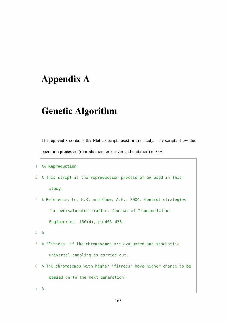
Appendix A
Genetic Algorithm
This appendix contains the Matlab scripts used in this study. The scripts show the
operation processes (reproduction, crossover and mutation) of GA.
1 %% Reproduction
2 % This script is the reproduction process of GA used in this
study.
3 % Reference: Lo, H.K. and Chow, A.H., 2004. Control strategies
for oversaturated traffic. Journal of Transportation
Engineering, 130(4), pp.466−478.
4 %
5 % 'Fitness' of the chromosomes are evaluated and stochastic
universal sampling is carried out.
6 % The chromosomes with higher 'fitness' have higher chance to be
passed on to the next generation.
7 %
163
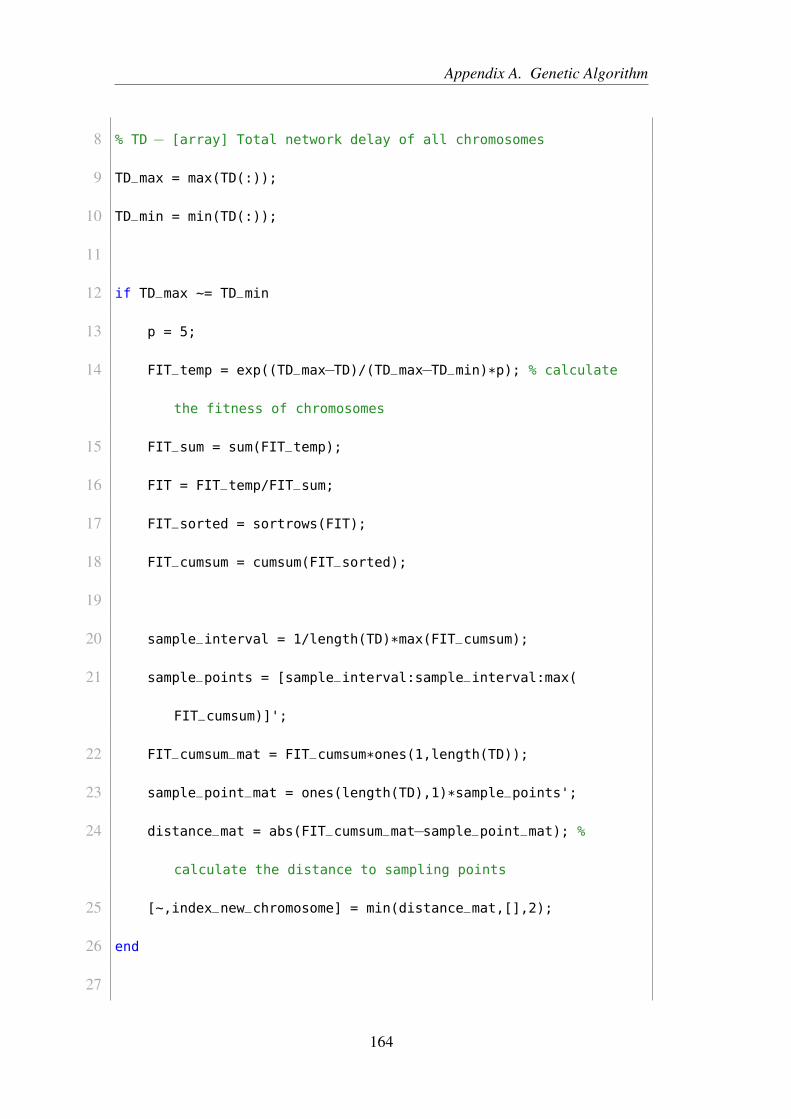
Appendix A. Genetic Algorithm
8 % TD − [array] Total network delay of all chromosomes
9 TD_max = max(TD(:));
10 TD_min = min(TD(:));
11
12 if TD_max ~= TD_min
13 p = 5;
14 FIT_temp = exp((TD_max−TD)/(TD_max−TD_min)*p); % calculate
the fitness of chromosomes
15 FIT_sum = sum(FIT_temp);
16 FIT = FIT_temp/FIT_sum;
17 FIT_sorted = sortrows(FIT);
18 FIT_cumsum = cumsum(FIT_sorted);
19
20 sample_interval = 1/length(TD)*max(FIT_cumsum);
21 sample_points = [sample_interval:sample_interval:max(
FIT_cumsum)]';
22 FIT_cumsum_mat = FIT_cumsum*ones(1,length(TD));
23 sample_point_mat = ones(length(TD),1)*sample_points';
24 distance_mat = abs(FIT_cumsum_mat−sample_point_mat); %
calculate the distance to sampling points
25 [~,index_new_chromosome] = min(distance_mat,[],2);
26 end
27
164

Appendix A. Genetic Algorithm
28
29 %% Crossover
30 % This script shows how GA's crossover process is implemented in
this study.
31 % Reference: Lo, H.K. and Chow, A.H., 2004. Control strategies
for oversaturated traffic. Journal of Transportation
Engineering, 130(4), pp.466−478.
32 %
33 % GA randomly choose two chromosomes as parent chromosomes.
34 % They will mate and produce two new children chromosomes.
35 % The crossover/mating process will randomly choose a crossover/
cut point.
36 % First part of parent 1 + second part of parent 2 = child 1
37 % First part of parent 2 + second part of parent 1 = child 2
38 % The procedure is continued until every chromosome is mated in
the new
39 % generation.
40 %
41 % Chromosome_parent − [structure array] parent chromosomes
42 % popNum − [constant] number of Chromosomes in test population
43 % croNum − [constant] number of crossover need to be carried out
44 % cycNum − [constant] number of cycle in the test period
45 % contrNum − [constant] number of controller in the network
165
Appendix A. Genetic Algorithm
46
47 croPair = randperm(popNum);
48 croPair = reshape(croPair,[croNum,2]); % pair up two random
Chromosomes for crossover process
49 Chromosome_child = Chromosome_parent;
50
51 for iCro = 1:croNum
52 for jCyc = 1:cycNum
53 for kContr = 1:contrNum
54 croPoint = randi([1 7]); % crossover point
55 int_A = Chromosome_child(croPair(iCro,1)).pop(jCyc,
kContr);
56 int_B = Chromosome_child(croPair(iCro,2)).pop(jCyc,
kContr);
57 bin_A = dec2bin(int_A,7); % convert integer into 7
bits binary string
58 bin_B = dec2bin(int_B,7);
59 cut_A = bin_A(croPoint:7);
60 cut_B = bin_B(croPoint:7);
61 bin_A(croPoint:7) = cut_B;
62 bin_B(croPoint:7) = cut_A;
63
64 Chromosome_child(croPair(iCro,1)).pop(jCyc,kContr) =
166
Appendix A. Genetic Algorithm
bin2dec(bin_A);
65 Chromosome_child(croPair(iCro,2)).pop(jCyc,kContr) =
bin2dec(bin_B);
66 end
67 end
68 end
69
70
71
72 %% Mutation
73 % This script is the reproduction process of GA used in this
study.
74 % Reference: Lo, H.K. and Chow, A.H., 2004. Control strategies
for oversaturated traffic. Journal of Transportation
Engineering, 130(4), pp.466−478.
75 %
76 % Chromosome − [structure array] include chromosomes of the
entire population
77 % popNum − [constant] number of Chromosomes in test population
78 % cycNum − [constant] number of cycle in the test period
79 % contrNum − [constant] number of controller in the network
80
81 mutRate = 0.005;
167
Appendix A. Genetic Algorithm
82 TotBits = popNum*cycNum*contrNum*7; % Total bits number of the
whole chromosome population
83 mutNum = round(TotBits*mutRate); % number of bits will be mutated
84 bits_loc = randperm(TotBits,mutNum); % bits locations for
mutation
85
86 for i = 1: length(bits_loc)
87 bit_temp = bits_loc(i);
88 bit_iPop = ceil(bit_temp/(cycNum*contrNum*7));
89 bit_temp = bit_temp−(bit_iPop−1)*(cycNum*contrNum*7);
90 bit_iCyc = ceil(bit_temp/(contrNum*7));
91 bit_temp = bit_temp−(bit_iCyc−1)*(contrNum*7);
92 bit_iContr = ceil(bit_temp/7);
93 bit_ind = bit_temp−(bit_iContr−1)*7;
94
95 bit_string = dec2bin(Chromosome(bit_iPop).pop(bit_iCyc,
bit_iContr),7);
96 switch bit_string(bit_ind)
97 case '1'
98 bit_string(bit_ind) = '0';
99 case '0'
100 bit_string(bit_ind) = '1';
101 end
168
Appendix A. Genetic Algorithm
102 Chromosome(bit_iPop).pop(bit_iCyc,bit_iContr) = bin2dec(
bit_string);
103 end
169
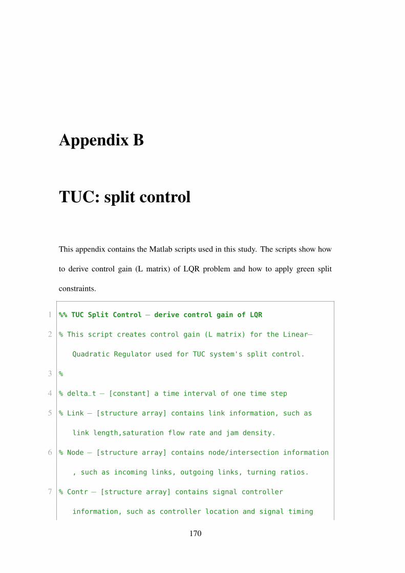
Appendix B
TUC: split control
This appendix contains the Matlab scripts used in this study. The scripts show how
to derive control gain (L matrix) of LQR problem and how to apply green split
constraints.
1 %% TUC Split Control − derive control gain of LQR
2 % This script creates control gain (L matrix) for the Linear−
Quadratic Regulator used for TUC system's split control.
3 %
4 % delta_t − [constant] a time interval of one time step
5 % Link − [structure array] contains link information, such as
link length,saturation flow rate and jam density.
6 % Node − [structure array] contains node/intersection information
, such as incoming links, outgoing links, turning ratios.
7 % Contr − [structure array] contains signal controller
information, such as controller location and signal timing
170
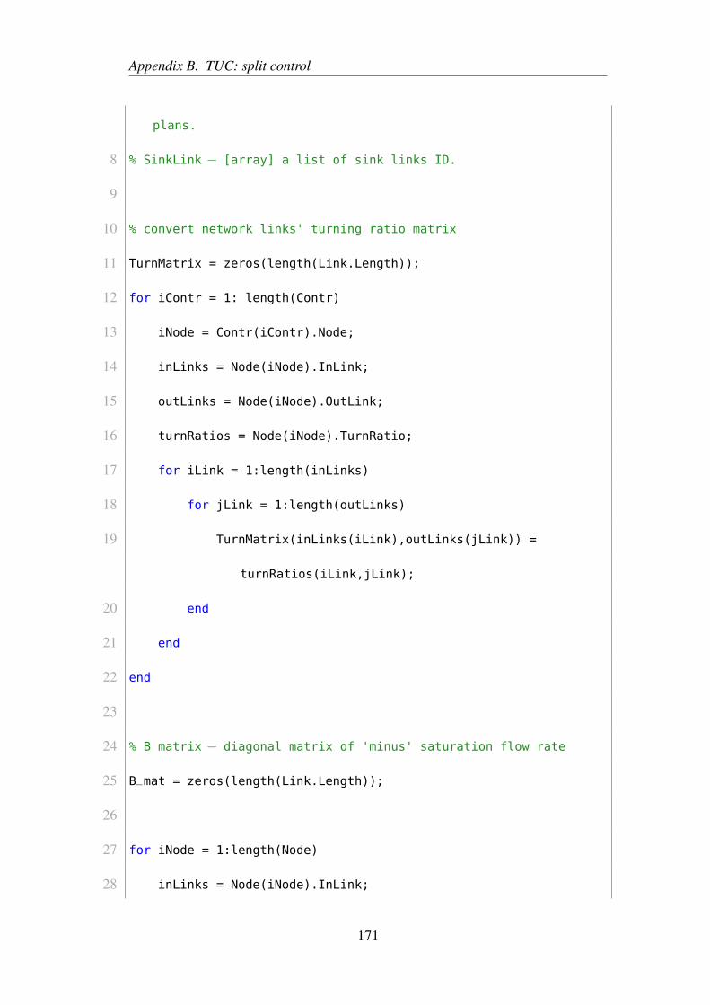
Appendix B. TUC: split control
plans.
8 % SinkLink − [array] a list of sink links ID.
9
10 % convert network links' turning ratio matrix
11 TurnMatrix = zeros(length(Link.Length));
12 for iContr = 1: length(Contr)
13 iNode = Contr(iContr).Node;
14 inLinks = Node(iNode).InLink;
15 outLinks = Node(iNode).OutLink;
16 turnRatios = Node(iNode).TurnRatio;
17 for iLink = 1:length(inLinks)
18 for jLink = 1:length(outLinks)
19 TurnMatrix(inLinks(iLink),outLinks(jLink)) =
turnRatios(iLink,jLink);
20 end
21 end
22 end
23
24 % B matrix − diagonal matrix of 'minus' saturation flow rate
25 B_mat = zeros(length(Link.Length));
26
27 for iNode = 1:length(Node)
28 inLinks = Node(iNode).InLink;
171
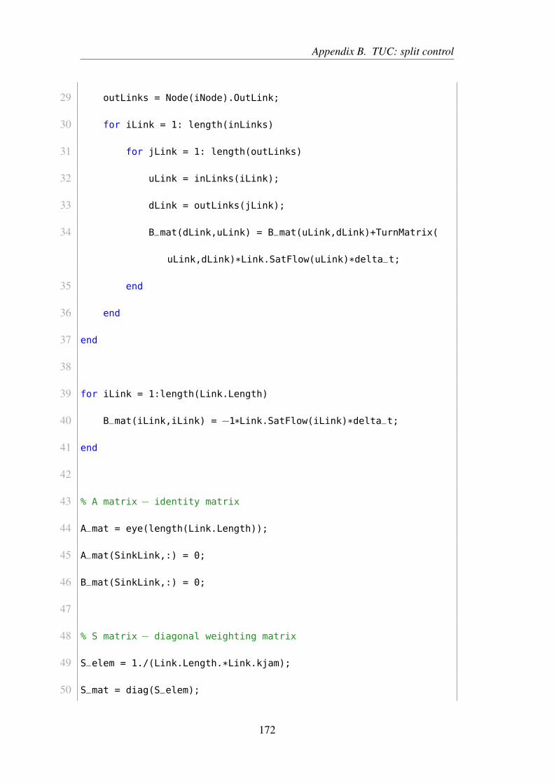
Appendix B. TUC: split control
29 outLinks = Node(iNode).OutLink;
30 for iLink = 1: length(inLinks)
31 for jLink = 1: length(outLinks)
32 uLink = inLinks(iLink);
33 dLink = outLinks(jLink);
34 B_mat(dLink,uLink) = B_mat(uLink,dLink)+TurnMatrix(
uLink,dLink)*Link.SatFlow(uLink)*delta_t;
35 end
36 end
37 end
38
39 for iLink = 1:length(Link.Length)
40 B_mat(iLink,iLink) = −1*Link.SatFlow(iLink)*delta_t;
41 end
42
43 % A matrix − identity matrix
44 A_mat = eye(length(Link.Length));
45 A_mat(SinkLink,:) = 0;
46 B_mat(SinkLink,:) = 0;
47
48 % S matrix − diagonal weighting matrix
49 S_elem = 1./(Link.Length.*Link.kjam);
50 S_mat = diag(S_elem);
172
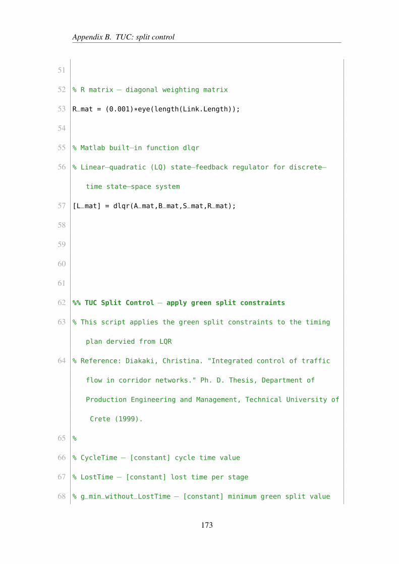
Appendix B. TUC: split control
51
52 % R matrix − diagonal weighting matrix
53 R_mat = (0.001)*eye(length(Link.Length));
54
55 % Matlab built−in function dlqr
56 % Linear−quadratic (LQ) state−feedback regulator for discrete−
time state−space system
57 [L_mat] = dlqr(A_mat,B_mat,S_mat,R_mat);
58
59
60
61
62 %% TUC Split Control − apply green split constraints
63 % This script applies the green split constraints to the timing
plan dervied from LQR
64 % Reference: Diakaki, Christina. "Integrated control of traffic
flow in corridor networks." Ph. D. Thesis, Department of
Production Engineering and Management, Technical University of
Crete (1999).
65 %
66 % CycleTime − [constant] cycle time value
67 % LostTime − [constant] lost time per stage
68 % g_min_without_LostTime − [constant] minimum green split value
173
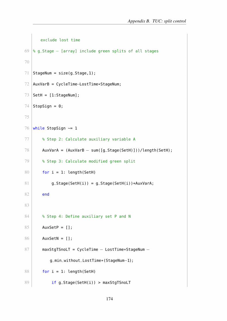
Appendix B. TUC: split control
exclude lost time
69 % g_Stage − [array] include green splits of all stages
70
71 StageNum = size(g_Stage,1);
72 AuxVarB = CycleTime−LostTime*StageNum;
73 SetH = [1:StageNum];
74 StopSign = 0;
75
76 while StopSign ~= 1
77 % Step 2: Calculate auxiliary variable A
78 AuxVarA = (AuxVarB − sum([g_Stage(SetH)]))/length(SetH);
79 % Step 3: Calculate modified green split
80 for i = 1: length(SetH)
81 g_Stage(SetH(i)) = g_Stage(SetH(i))+AuxVarA;
82 end
83
84 % Step 4: Define auxiliary set P and N
85 AuxSetP = [];
86 AuxSetN = [];
87 maxStgTSnoLT = CycleTime − LostTime*StageNum −
g_min_without_LostTime*(StageNum−1);
88 for i = 1: length(SetH)
89 if g_Stage(SetH(i)) > maxStgTSnoLT
174
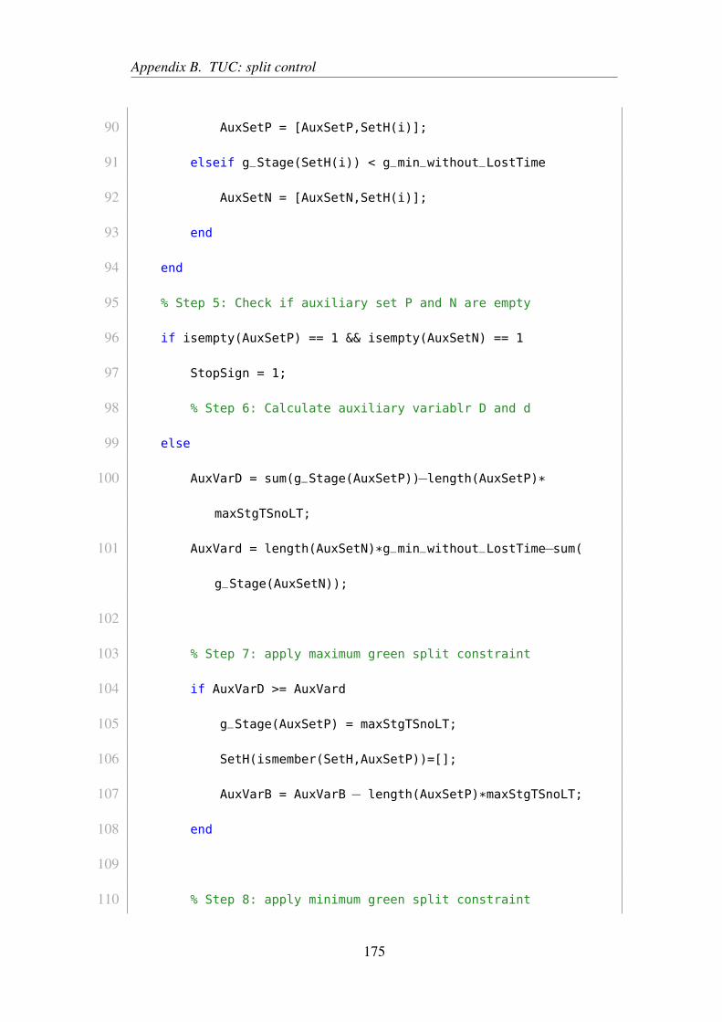
Appendix B. TUC: split control
90 AuxSetP = [AuxSetP,SetH(i)];
91 elseif g_Stage(SetH(i)) < g_min_without_LostTime
92 AuxSetN = [AuxSetN,SetH(i)];
93 end
94 end
95 % Step 5: Check if auxiliary set P and N are empty
96 if isempty(AuxSetP) == 1 && isempty(AuxSetN) == 1
97 StopSign = 1;
98 % Step 6: Calculate auxiliary variablr D and d
99 else
100 AuxVarD = sum(g_Stage(AuxSetP))−length(AuxSetP)*
maxStgTSnoLT;
101 AuxVard = length(AuxSetN)*g_min_without_LostTime−sum(
g_Stage(AuxSetN));
102
103 % Step 7: apply maximum green split constraint
104 if AuxVarD >= AuxVard
105 g_Stage(AuxSetP) = maxStgTSnoLT;
106 SetH(ismember(SetH,AuxSetP))=[];
107 AuxVarB = AuxVarB − length(AuxSetP)*maxStgTSnoLT;
108 end
109
110 % Step 8: apply minimum green split constraint
175
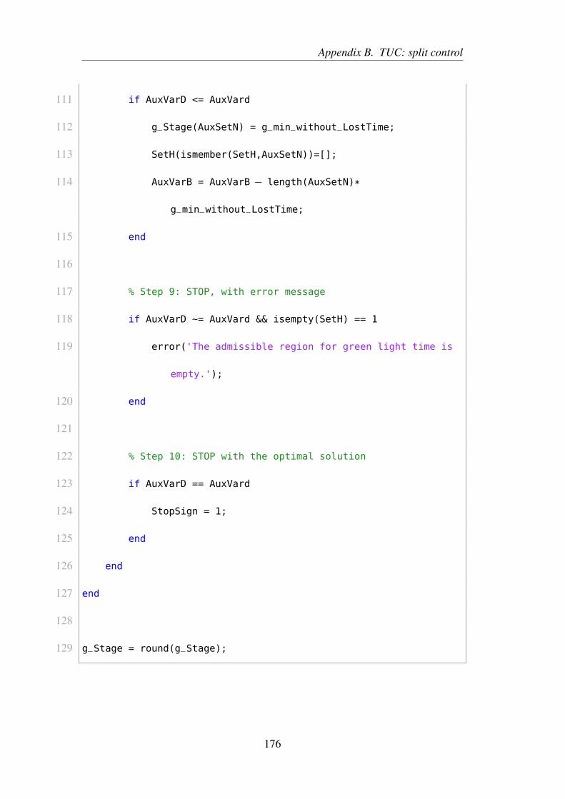
Appendix B. TUC: split control
111 if AuxVarD <= AuxVard
112 g_Stage(AuxSetN) = g_min_without_LostTime;
113 SetH(ismember(SetH,AuxSetN))=[];
114 AuxVarB = AuxVarB − length(AuxSetN)*
g_min_without_LostTime;
115 end
116
117 % Step 9: STOP, with error message
118 if AuxVarD ~= AuxVard && isempty(SetH) == 1
119 error('The admissible region for green light time is
empty.');
120 end
121
122 % Step 10: STOP with the optimal solution
123 if AuxVarD == AuxVard
124 StopSign = 1;
125 end
126 end
127 end
128
129 g_Stage = round(g_Stage);
176
References
[1] United Nations. Department of Economic and Social Affairs. Population Di-
vision. World Urbanization Prospects: The 2014 Revision. UN, 2015.
[2] Department for Transport. Road traffic forecasts 2015. [Accessed on: 10 Jan
2016].
[3] INRIX. INRIX traffic scorecard. http://inrix.com/scorecard/, 2016.
[Accessed on: 19 Jun 2017].
[4] A.H.F. Chow, A. Santacreu, I. Tsapakis, G. Tanasaranond, and T. Cheng. Em-
pirical assessment of urban traffic congestion. Journal of Advanced Trans-
portation, 48(8):1000–1016, 2014.
[5] Siemens PLC Peek Traffic Ltd and TRL Limited. SCOOT.
[6] T. Le, P. Kovács, N. Walton, H.L. Vu, L.L.H. Andrew, and S.S.P. Hoogen-
doorn. Decentralized signal control for urban road networks. Transportation
Research Part C: Emerging Technologies, 2015.
[7] J. Li and M.H. Zhang. Coupled linear programming approach for decentral-
177
References
ized control of urban traffic. Transportation Research Record: Journal of the
Transportation Research Board, (2439):83–93, 2014.
[8] P. Varaiya. The max-pressure controller for arbitrary networks of signalized
intersections. Springer, 2013.
[9] H. Prothmann, S. Tomforde, J. Branke, J. Hähner, C. Müller-Schloer, and
H. Schmeck. Organic traffic control. Springer, 2011.
[10] S. Lammer and D. Helbing. Self-control of traffic lights and vehicle flows in
urban road networks. Journal of Statistical Mechanics: Theory and Experi-
ment, P04019, 2008.
[11] L.B. de Oliveira and E. Camponogara. Multi-agent model predictive control
of signaling split in urban traffic networks. Transportation Research Part C:
Emerging Technologies, 18(1):120–139, 2010.
[12] A.H.F. Chow. Optimisation of dynamic motorway traffic via a parsimonious
and decentralised approach. Transportation Research Part C, 55:69–84, 2015.
[13] J.J. Olstam and A. Tapani. Comparison of car-following models. Technical
report, 2004.
[14] R.E. Chandler, R. Herman, and E.W. Montroll. Traffic dynamics: studies in
car following. Operations Research, 6(2):165–184, 1958.
[15] D.C. Gazis, R. Herman, and R.B. Potts. Car-following theory of steady-state
traffic flow. Operations Research, 7(4):499–505, 1959.
178
References
[16] D.C. Gazis, R. Herman, and R.W. Rothery. Nonlinear follow-the-leader mod-
els of traffic flow. Operations Research, 9(4):545–567, 1961.
[17] A.D. May. Non-integer car-following models. Highway Research Record,
199(3):19–32, 1967.
[18] H. Ozaki. Reaction and anticipation in the car-following behavior. In Pro-
ceedings of the 13th International Symposium on the Theory of Road Traffic
Flow, pages 349–366, 1993.
[19] M. Brackstone and M. McDonald. Car-following: a historical review. Trans-
portation Research Part F: Traffic Psychology and Behaviour, 2(4):181–196,
1999.
[20] L.A. Pipes. An operational analysis of traffic dynamics. Journal of Applied
Physics, 24(3):274–281, 1953.
[21] S.P. Hoogendoorn and P.H.L. Bovy. State-of-the-art of vehicular traffic flow
modelling. Proceedings of the Institution of Mechanical Engineers, Part I:
Journal of Systems and Control Engineering, 215(4):283–303, 2001.
[22] W. Leutzbach. Introduction to the theory of traffic flow. Springer, 1988.
[23] G.F. Newell. A simplified car-following theory: a lower order model. Trans-
portation Research Part B: Methodological, 36(3):195–205, 2002.
[24] L. Leclercq. Hybrid approaches to the solutions of the âAIJlighthill–
whitham–richardsâAI model. Transportation Research Part B: Methodologi-
cal, 41(7):701–709, 2007.
179
References
[25] R. Wiedemann. Simulation des strassenverkehrsflusses. Technical report,
1974.
[26] PTV Group. VISSIM 5.40 user manual, 2011.
[27] B.D. Greenshields, J.R. Bibbins, W.S. Channing, and H.H. Miller. A study
of traffic capacity. In Proceedings of the 14th annual meeting of the highway
research board, volume 14, pages 448–477, 1935.
[28] H. Greenberg. An analysis of traffic flow. Operations Research, 7(1):79–85,
1959.
[29] L.C. Edie. Car-following and steady-state theory for noncongested traffic.
Operations Research, 9(1):66–76, 1961.
[30] G. F. Newell. A simplified theory of kinematic waves in highway traffic: I
general theory, ii queuing at freeway bottlenecks, iii: multi-destination flows.
Transportation Research Part B, 27:281–313, 1993.
[31] C. F. Daganzo. The cell transmission model: A dynamic representation of
highway traffic consistent with the hydrodynamic theory. Transportation Re-
search Part B: Methodological, 28(4):269–287, 1994.
[32] M.J. Lighthill and G.B. Whitham. On kinematic waves. ii. a theory of traffic
flow on long crowded roads. In Proceedings of the Royal Society of London A:
Mathematical, Physical and Engineering Sciences, volume 229, pages 317–
345. The Royal Society, 1955.
180
References
[33] P.I. Richards. Shock waves on the highway. Operations Research, 4(1):42–51,
1956.
[34] S.K. Godunov. A difference method for numerical calculation of discontin-
uous solutions of the equations of hydrodynamics. Matematicheskii Sbornik,
89(3):271–306, 1959.
[35] H.J. Payne. Models of freeway traffic and control. Mathematical models of
public systems, pages 51–61, 1971.
[36] M. Papageorgiou, J.M. Blosseville, and H. Hadj-Salem. Modelling and real-
time control of traffic flow on the southern part of boulevard peripherique
in paris: Part i: Modelling. Transportation Research Part A: General,
24(5):345–359, 1990.
[37] D. Helbing. Gas-kinetic derivation of navier-stokes-like traffic equations.
Physical Review E, 53(3):2366, 1996.
[38] M. Papageorgiou. Some remarks on macroscopic traffic flow modelling.
Transportation Research Part A: Policy and Practice, 32(5):323–329, 1998.
[39] F.V. Webster. Traffic signal settings. Technical report, 1958.
[40] Dennis I Robertson. Transyt: a traffic network study tool. 1969.
[41] Transport Research Laboratory. TRANSYT - Traffic Network and Isolated
Intersection Study Tool (Version 15). trlsoftware.co.uk/products/
junction_signal_design/transyt, 2015. [Accessed on: 30 Jul 2015].
181
References
[42] N.H. Gartner, J.D.C. Little, and H. Gabbay. Mitrop: a computer program for
simultaneous optimisation of offsets, splits and cycle time. Traffic Engineer-
ing & Control, 17(8/9), 1976.
[43] K.W. Huddart and E.D. Turner. Traffic signal progression - GLC combination
method. Traffic Engineering & Control, 8(8), 1969.
[44] M.C. Bell and R.D. Bretherton. Ageing of fixed-time traffic signal plans. In
International Conference On Road Traffic Control, 1986.
[45] D. Robertson and R. Bretherton. Optimizing networks of traffic signals in
real time-the scoot method. IEEE Transactions on Vehicular Technology,
40(1):11–15, 1991.
[46] P.B. Hunt, D.I. Robertson, R.D. Bretherton, and R.I. Winton. Scoot-a traffic
responsive method of coordinating signals. Technical report, 1981.
[47] P.R. Lowrie. The sydney coordinated adaptive traffic system-principles,
methodology, algorithms. In International Conference on Road Traffic Sig-
nalling, 1982, London, United Kingdom, number 207, 1982.
[48] Roads and Maritime Services. An introduction to SCATS: SCATS
6 âAS functional description. http://www.scats.com.au/files/an_
introduction_to_scats_6.pdf, 2011. [Accessed on: 30 Oct 2015].
[49] N.H. Gartner. OPAC: A demand-responsive strategy for traffic signal control.
Number 906. 1983.
182
References
[50] L.C. Liao. A review of the optimized policies for adaptive control strategy
(OPAC). California PATH Program, Institute of Transportation Studies, Uni-
versity of California at Berkeley, 1998.
[51] P. Mirchandani and L. Head. A real-time traffic signal control system: archi-
tecture, algorithms, and analysis. Transportation Research Part C: Emerging
Technologies, 9(6):415 – 432, 2001.
[52] P. Mirchandani and F. Wang. RHODES to intelligent transportation systems.
Intelligent Systems, IEEE, 20(1):10–15, Jan 2005.
[53] C. Diakaki. Integrated control of traffic flow in corridor networks. PhD thesis,
Technical University of Crete, 1999.
[54] C. Diakaki, M. Papageorgiou, and K. Aboudolas. A multivariable regular ap-
proach to traffic responsive network-wide signal control. Control Engineering
Practice, 10:183–195, 2002.
[55] UTOPIA: Optimizing traffic flows across the road network. https://www.
swarco.com/mizar-en/Products/Urban-Systems/UTOPIA. [Accessed
on: 23 Oct 2015].
[56] UTOPIA - Urban traffic control system architecture. http://ftp.
citilabs.com/sites/default/files/files/3_Swarco.pdf. [Accessed
on: 23 Oct 2015].
[57] M. Rinaldi and C.M.J. Tampère. An extended coordinate descent method for
183
References
distributed anticipatory network traffic control. Transportation Research Part
B: Methodological, 80:107–131, 2015.
[58] N.E. Marinica. Distributed estimation and control of interacting hybrid sys-
tems for traffic applications. PhD thesis, Ghent University, 2014.
[59] S. Lämmer and D. Helbing. Self-stabilizing decentralized signal control of
realistic, saturated network traffic. Santa Fe Institute, 2010.
[60] R.T. Van Katwijk. Multi-agent look-ahead traffic-adaptive control. PhD the-
sis, Delft University of Technology, 2008.
[61] T. Wongpiromsarn, T. Uthaicharoenpong, Y. Wang, E. Frazzoli, and D. Wang.
Distributed traffic signal control for maximum network throughput. In Intel-
ligent Transportation Systems (ITSC), 2012 15th International IEEE Confer-
ence on, pages 588–595. IEEE, 2012.
[62] M.R. Crabtree. MOVA traffic control manual. Application guide:Issue D,
2011.
[63] Hong Lo. A novel traffic signal control formulation. Transportation Research
Part B, 33:433 – 448, 1999.
[64] G. Gomes and R. Horowitz. Optimal freeway ramp metering using the asym-
metric cell transmission model. Transportation Research Part C, 14(4):244 –
262, 2006.
[65] K. Aboudolas, M. Papageorgiou, and E. Kosmatopoulos. Store-and-forward
184
References
based methods for the signal control problem in large-scale congested urban
road networks. Transportation Research Part C, 17:163–174, 2009.
[66] S. Timotheou, C.G. Panayiotou, and M.M. Polycarpou. Network traffic sig-
nal control with nonconvex alternating direction method of multipliers for-
mulations. Transportation Research Record: Journal of the Transportation
Research Board, (2490):11–20, 2015.
[67] N.H. Gartner, S.F. Assman, F. Lasaga, and D.L. Hou. A multi-band ap-
proach to arterial traffic signal optimization. Transportation Research Part
B: Methodological, 25(1):55–74, 1991.
[68] N.H. Gartner and C. Stamatiadis. Arterial-based control of traffic flow in
urban grid networks. Mathematical and computer modelling, 35(5-6):657–
671, 2002.
[69] J.H. Holland. Adaptation in natural and artificial systems. 1975. Ann Arbor,
MI: University of Michigan Press and, 1992.
[70] H. Lo and A. H. F. Chow. Control strategies for over-saturated traffic. ASCE
Journal of Transportation Engineering, 130:466–478, 2004.
[71] TRAVOLUTION in Ingolstadt. http://www.travolution-ingolstadt.
de. [Accessed on: 21 Oct 2015].
[72] M. Dorigo, V. Maniezzo, and A. Colorni. Ant system: optimization by a
colony of cooperating agents. IEEE Transactions on Systems, Man, and Cy-
bernetics, Part B (Cybernetics), 26(1):29–41, 1996.
185
References
[73] R. Putha, L. Quadrifoglio, and E. Zechman. Comparing ant colony optimiza-
tion and genetic algorithm approaches for solving traffic signal coordination
under oversaturation conditions. Computer-Aided Civil and Infrastructure En-
gineering, 27(1):14–28, 2012.
[74] J. Wu, A. Abbas-Turki, and A. El Moudni. Cooperative driving: an ant
colony system for autonomous intersection management. Applied Intelli-
gence, 37(2):207–222, 2012.
[75] Z. Cong, B. De Schutter, and R. Babuška. Ant colony routing algorithm for
freeway networks. Transportation Research Part C: Emerging Technologies,
37:1–19, 2013.
[76] F. Glover. Future paths for integer programming and links to artificial intelli-
gence. Computers & operations research, 13(5):533–549, 1986.
[77] F. Glover and M. Laguna. Tabu SearchâLU. Springer, 2013.
[78] T. Hu and L. Chen. Traffic signal optimization with greedy randomized tabu
search algorithm. Journal of Transportation Engineering, 138(8):1040–1050,
2012.
[79] N. Metropolis, A.W. Rosenbluth, M.N. Rosenbluth, A.H. Teller, and E. Teller.
Equation of state calculations by fast computing machines. The journal of
chemical physics, 21(6):1087–1092, 1953.
[80] S. Memoli, G.E. Cantarella, S. de Luca, and R. Di Pace. Network signal
186
References
setting design with stage sequence optimisation. Transportation Research
Part B: Methodological, 100:20–42, 2017.
[81] F. Glover, M. Laguna, E. Taillard, and D. de Werra. Tabu search. Baltzer
Basel, 1993.
[82] H. Lo and A.H.F. Chow. Control strategies for over-saturated traffic. ASCE
Journal of Transportation Engineering, 130:466–478, 2004.
[83] W.B. Powell. Approximate Dynamic Programming - Solving the Curses of
Dimensionality. Wiley, Hoboken, New Jersey, 2010.
[84] A.H.F. Chow, S. Li, W.Y. Szeto, and D.Z.W. Wang. Modelling urban traffic
dynamics based upon the variational formulation of kinematic waves. Trans-
portmetrica B, 3(3):169–191, 2015.
[85] A. H. F. Chow, A Santacreu, I Tsapakis, G Tanasaranond, and T Cheng. Em-
pirical assessment of urban traffic congestion. Journal of Advanced Trans-
portation, 48(8):1000 – 1016, 2014.
[86] R. Sanchez, R. Horowitz, and P. Varaiya. Analysis of queue estimation
methods using wireless magnetic sensors. Transportation Research Record,
2229:34–45, 2011.
[87] D.C. Gazis. Traffic theory, volume 50. Springer Science & Business Media,
2002.
[88] C. Diakaki, V. Dinopoulou, K. Aboudolas, M. Papageorgiou, E. Ben-Shabat,
E. Seider, and A. Leibov. Extensions and new applications of the traffic-
187
References
responsive urban control strategy: coordinated signal control for urban net-
works. Transportation Research Record, 1856:202–211, 2003.
[89] C. Diakaki, V. Dinopoulou, K. Aboudolas, M. Papageorgiou, E. Ben-Shabat,
E. Seider, and A. Leibov. Extensions and new applications of the traffic-
responsive urban control strategy: coordinated signal control for urban net-
works. Transportation Research Record, 1856:202–211, 2003.
[90] A. Kouvelas, K. Aboudolas, M. Papageorgiou, and E. Kosmatopoulos. A
hybrid strategy for real-time traffic signal control of urban road networks.
IEEE Transactions on Intelligent Transportation Systems, 12:884–894, 2011.
[91] M. J. Smith. A local traffic control policy which automatically maximises
the overall travel capacity of an urban road network. Traffic Engineering and
Control, 21(6):298–302, 1980.
[92] A. Kouvelas, J. Lioris, S. Fayazi, and P. Varaiya. Maximum pressure con-
troller for stabilizing queues in signalized arterial networks. Transportation
Research Record, 2421:133–141, 2014.
[93] L. Tassiulas and A. Ephremides. Stability properties of constrained queueing
systems and scheduling policies for maximum throughput in multihop radio
networks. IEEE transactions on automatic control, 37(12):1936–1948, 1992.
[94] K. Aboudolas, M. Papageorgiou, A. Kouvelas, and E. Kosmatopoulos. A
rolling-horizon quadratic-programming approach to the signal control prob-
lem in large-scale congested urban road networks. Transportation Research
Part C, 18:680–694, 2010.
188
References
[95] T. Le, P. Kovacs, N. Walton, H. Vu, and L. Andrew. Decentralised signal
control for urban road networks. Transportation Research Part C, 58:431–
450, 2015.
[96] R. Sanchez, R. Horowitz, and P. Varaiya. Analysis of queue estimation
methods using wireless magnetic sensors. Transportation Research Record,
2229:34–45, 2011.
[97] D. Krajzewicz, J. Erdmann, M. Behrisch, and L. Bieker. Recent development
and applications of sumo - simulation of urban mobility. International Jounral
on Advanced in Systems and Measurements, 5(3&4), 2012.
[98] D. Krajzewicz. Traffic Simulation with SUMO âAS Simulation of Urban Mo-
bility, volume 145. Springer, 2010.
[99] S. Krauss. Microscopic modeling of traffic flow: Investigation of collision free
vehicle dynamics. PhD thesis, Universitat zu Koln., 1998.
[100] R.E. Allsop. Some possibilities for using traffic control to influence trip distri-
bution and route choice. In Transportation and Traffic Theory, Proceedings,
volume 6, 1974.
[101] M.J. Smith. Traffic control and route-choice; a simple example. Transporta-
tion Research Part B: Methodological, 13(4):289–294, 1979.
[102] R. Liu and M. Smith. Route choice and traffic signal control: A study of the
stability and instability of a new dynamical model of route choice and traffic
189
References
signal control. Transportation Research Part B: Methodological, 77:123–145,
2015.
[103] M. J. Smith, R. Liu, and R. Mounce. Traffic control and route choice: Capac-
ity maximisation and stability. Transportation Research Part B: Methodolog-
ical, 81:863–885, 2015.
[104] B. G. Heydecker and J. D. Addison. Analysis of dynamic traffic equilibrium
with departure time choice. Transportation Science, 39(1):39–57, 2005.
[105] A.H.F. Chow, K. Han, and K. Achuthan. An agent-based analysis of transport
network vulnerability and resilience with provision of travel information. In
The Sixth International Symposium on Dynamic Traffic Assignment, 2016.
[106] TraCI4Matlab: A implementation of the traci interface for mat-
lab. http://uk.mathworks.com/matlabcentral/fileexchange/
44805-traci4matlab?requestedDomain=www.mathworks.com, note =
[Accessed on: 17 Oct 2017].
[107] A.H.F. Chow and R. Sha. Performance analysis of centralized and distributed
systems for urban traffic control. Transportation Research Record: Journal
of the Transportation Research Board, (2557):66–76, 2016.
[108] OpenStreetMap. http://www.openstreetmap.org/. [Accessed on: 30 Oct
2017].
[109] J.D.C. Little, M.D. Kelson, and N.H. Gartner. Maxband: A program for set-
190
References
ting signals on arterials and triangular networks. In Transportation Research
Record 795, pages 40–46. TRB, 1981.
[110] N.H. Gartner, S.F. Assmann, F. Lasaga, and D.L. Hous. Multiband–a variable-
bandwidth arterial progression scheme. Number 1287, 1990.
[111] T. Arsava, Y. Xie, and N.H. Gartner. Arterial progression optimization us-
ing od-band: Case study and extensions. Transportation Research Record:
Journal of the Transportation Research Board, (2558):1–10, 2016.
[112] E. Camponogara and H.F. Scherer. Distributed optimization for model pre-
dictive control of linear dynamic networks with control-input and output
constraints. IEEE Transactions on Automation Science and Engineering,
8(1):233–242, 2011.
[113] J. Haddad, B. De Schutter, D. Mahalel, I. Ioslovich, and P. Gutman. Optimal
steady-state control for isolated traffic intersections. IEEE Transactions on
automatic control, 55(11):2612–2617, 2010.
[114] J. Reilly and A.M. Bayen. Distributed optimization for shared state systems:
applications to decentralized freeway control via subnetwork splitting. IEEE
Transactions on Intelligent Transportation Systems, 16(6):3465–3472, 2015.
[115] M. Rinaldi, W. Himpe, and C.M.J. Tampère. A sensitivity-based approach for
adaptive decomposition of anticipatory network traffic control. Transporta-
tion Research Part C: Emerging Technologies, 66:150–175, 2016.
191


