Design considerations for closed circuits of drip irrigation system. PhD: Thesis, Faculty of Agriculture, Agric., Ain Shams university, Egypt

DESIGN CONSIDERATIONS FOR CLOSED-CIRCUITS OF DRIP IRRIGATION

SYSTEM

By

HANI ABDEL-GHANI ABDEL-GHANI MANSOUR

B.Sc. Agric. Sc. (Agricultural Engineering), Menoufia University, 2000.

M.Sc. Agric. Sc. (Agricultural Mechanization), Ain Shams University, 2006.

A thesis submitted in partial fulfillment

of

the requirements for the degree of

DOCTOR OF PHILOSOPHY

in

Agricultural Science

(Agricultural Mechanization)

Department of Agricultural Engineering

Faculty of Agriculture

Ain Shams University

2012

DESIGN CONSIDERATIONS FOR CLOSED-CIRCUITS OF DRIP IRRIGATION

SYSTEM

By

HANI ABDEL-GHANI ABDEL-GHANI MANSOUR

B.Sc. Agric. Sc. (Agricultural Engineering), Menoufia University, 2000.

M.Sc. Agric. Sc. (Agricultural Mechanization), Ain Shams University, 2006.

Under the supervision of:

Dr. Abdel Ghany Mohamed El-Gindy Prof. Emeritus of Agriculture Engineering, Department of

Agricultural Engineering, Faculty of Agriculture, Ain Shams

University. (Principal Supervisor)

Dr. Mohamed Youssef Tayel

Prof. Emeritus, of Water Relations and Soil Physics, Department of

Water Relations and Field Irrigation, Agricultural and Biology

Research Division, National Research Centre.

Dr. David Anthony Lightfoot

Prof. of Plant, Soil and Agricultural Systems, Department of Plant &

Soil and Agricultural Systems, Faculty of Agriculture, Southern

Illinois University.

ABSTRACT

Hani Abdel-Ghani Abdel-Gani Mansour: Design

Considerations for Closed Circuits of Drip Irrigation System.

Unpublished Ph.D. Thesis, Department of Agricultural Engineering,

Faculty of Agriculture, Ain Shams University, 2012.

Egypt, as country of the arid region (modest precipitation of 100-

200 mm year-1

), will face a scarce of irrigation water, due to increase

population and need more food, so maximizing of available one is a must,

especially under localized irrigation system. Such as trickle irrigation

system which the main disadvantages is pressure reduction at the end of

lateral lines. Closed circuits are considered one of the modifications of

trickle irrigation system, and will add advantages to traditional trickle

irrigation because it can relieve low operating pressures problem at the

end of the lateral lines.

The objectives of the present research were: Studying the effect of

different trickle irrigation circuits (one manifold line (CM1DIS), two

manifold lines (CM2DIS) and traditional trickle system (TDIS) as a

control) ,and lateral line lengths (LLL1= 40 m, LLL2= 60 m and LLL3= 80

m) on : i) some hydraulic parameters, ii) corn (Zea Mays-L) crop

productivity, water use efficiency (WUE), fertilizers use efficiency

(FUE), and iii) cost analysis of corn production.

PE tubes lateral lines: Ø16 mm; 30 cm distance, and built-in

emitters 4 lh-1

at operating pressure 101.325 kPa. Laboratory tests were

conducted at the Agric. Eng. Res. Inst., ARC, MALR, Egypt. Whereas

field experiment was conducted at the Experimental Farm of Faculty of

Agriculture, Southern Illinois University at Carbondale (SIUC).

Results could be summarized as following:

According to pressure head(m), uniformity coefficient (%) and

emitters discharge (lh-1

) of trickle irrigation circuits (DIC), it they could

be ranked in the following descending order: CM2DIS > CM1DIS > TDIS,

meanwhile lateral line lengths (LLL) could be ranked in following

descending order: LLL1= (40 m) > LLL2= (60 m) > LLL3= (80 m). In

respect to friction loss and coefficient of variation, DIC and LLL could be

ranked opposite the previous orders. With respect to flow velocity (ms-1

),

velocity head (m) and lateral discharge (lh-1

), DIC and LLL could be

ranked in the following descending orders: CM2DIS>CM1DIS>TDIS and

LLL3>LLL2>LLL1, respectively. According to the validation of predicted

and measured energy head loss, the regression analysis between predicted

and measured values were significantly at the 1 % level, under different

DIC and LLL treatments. Concerning to vegetative growth parameters:

one leaf area (cm2), plant height (cm), leaf length (cm) and number of

leaves plant-1

, DIC and LLL, used them could be arranged in the

following descending orders: CM2DIS > CM1DIS > TDIS and CM2DIS >

CM1DIS > TDIS under, respectively. According to grain and Stover water

use efficiency and fertilizers use efficiency, DIC and LLL were used

could be arranged in the following descending orders: CM2DIS >

CM1DIS > TDIS and CM2DIS > CM1DIS > TDIS under, respectively.

Cost analysis indicated that modified circuits DIC, CM2DIS and CM1DIS,

meanwhile the shorter LLL, LLL1 and LLL2 achieved the highest values

of revenue net profits, economic net income from irrigation water and

physical net income from irrigation water.

Keywords: Trickle irrigation, Circuits, Manifolds, Laterals, Friction loss,

Flow velocity, Uniformity coefficient, Corn growth, Yield, Cost analysis.

ACKNOWLEDGMENT

Thanks to ALLAH for his gracious kindness in all endeavors the author

has taken up in his life.

I wish to express my deep appreciation and gratitude to supervisor Prof.

Dr. Abdel Ghany M. El-Gindy, Prof. of Agric. Eng., Faculty of Agriculture, Ain

Shams University, and Prof. Dr. Mohamed Youssef Tayel, Prof. of Soil Physics

and Soil Water Relations, Water Relations and Field Irrigation Dept., Agric. &

Bilo. Div., NRC, for problem suggestion, supervision, encouragement, valuable,

advices and manuscript supervision and reviewing, frequent discussions

throughout the study.

I like also to thank the Co-supervisor Prof. Dr. David Anthony

Lightfoot, Professor, Plant & Soil and Agriculture system Dept., Fac. of Agric.,

Southern Illinois University at Carbondale (SIUC), Illinois, USA. for his

valuable help and advices throughout this work. And due thanks and indebted to

Prof. Dr. Mohamed Abd El-Hady Abd El-Hamid, Prof. of Soil Physics and

Water Relations, Water Relations and Field Irrigation, Dept., Agric. & Bilo.

Div., NRC.

Special thanks to Egyptian Ministry of Higher Education and Scientific

Research for giving me the opportunity to travel and stay in USA on a mission to

complete part of the practical side of this thesis, all staff members Water

Relations and Field Irrigation, N.R.C, all Staff members of the Dept., of Agric.

Eng., Fac. of Agric, Ain Shams Univ., members of Agric. Eng. Res. Inst., A.R.C,

and all staff members of Soil and Plant and Agric. Systems Dept., SIUC for their

support and personal encouragement, valuable help in this work.

Finally, I wish to express my deepest appreciation to my family (spirit of

my mother), my father, my wife, and my three children, for their continuous

encouragement and support.

Contents

Page Subject

1 I. INTRODUCTION………………………………………..…….………….... 4 II. REVIEW OF LITERATURE……………………….….……....................

15 III. MATERIALS AND METHODS…………………………...……... 37 IV. RESULTS AND DISSCUSION……………………………..…..………..

37 4-1. Effect of trickle irrigation circuits (DIC) and lateral line length (LLL) on

pressure head and some hydraulic characteristics (operating pressure = 1

atm and slope = 0%)………………............................................................

37 4.1.1. Pressure head…………………………..………………………..…....

44 4.1.2. Friction loss…………………………………………..…………….…

47 4.1.3. Flow velocity ………………………………………………………..

49 4.1.4. Velocity head……………………………………………………...

51 4.1.5. Emitter discharge and variations ……..……………………………..

54 4.1.6. Lateral line discharge…………………………………………………

56 4.1.7. Uniformity coefficient......................................................................

58 4-1-8. Coefficient of variation for emitter discharge………........................

61 4-1-9. Comparing the practical data of head loss along the lateral line in the

laboratory with those calculated using HydroCalc simulation

program …………………………………………………………….

69

4-2. Effect of DIC and LLL on vegetative growth and yield parameters of corn

crop………………………………………………………………………..

69 4-2-1. Leaf area ……..………………………..…………….......................

69

72

72

4-2-2. Plant height …………………………………………………………

4-2-3. Leaf length ……………………………………………………….....

4-2-4. Number of leaves per plant………………………………………...

73 4-2-5. Grain yield…………………………………………………………..

73 4-2-6. Stover yield…...…………………………………………………….

74 4-3. Effect of different trickle irrigation closed-circuits and lateral line lengths

on grain and stover water use efficiency………………………………

76 4-4. Effect of different trickle irrigation closed-circuits and lateral line lengths

on fertilizers use efficiency ……………………………………………

78 4-5. Effect of trickle irrigation circuits and lateral lines length on costs analysis

of corn production………………………………………………………

83 V. SUMMARY………………………………………………….......................

92 VI. REFERENCES……………………………………………….……………

103 VII. Annex …………………………………………………………..………….

VIII. Arabic summary…………………………………………………......…..

II

List of tables

Title Page

Table (1): Methods of comparison of statistical uniformity (ASAE,

1999).…………………………………………………………...

7

Table (2): Some soil physical properties of Carbondale, Illinois site……... 16

Table (3): Some soil chemical properties of Carbondale, Illinois site……... 16

Table (4): Some chemical data of irrigation water at Carbondale, Illinois,

USA……………………………………………………………...

17

Table (5): Percentage of soil wetted by various discharges and spacings for a

single row of uniformly spaced distributors in a straight line

applying 40mm of water per cycle over the wetted area………

30

Table (6): Water requirements for Maize grown at Carbondale site, IL., USA,

2010.…………………………………….………..……………..

31

Table (7): Effect of trickle irrigation closed-circuits (DIC) and lateral line

lengths (LLL) on some hydraulic parameters of lateral lines under

(operating pressure = 1 atm and slope = 0%)………………….

39

Table (8): Effect of trickle irrigation closed-circuits (DIC) and lateral line

lengths (LLL) pressure head variation…................................... 44

Table (9): Effect of DIC design and LLL on emitter qvar percent.................. 51

Table (10): Effect of different irrigation circuits design and lateral lines lengths

on both emitters; lateral discharge and uniformity under (operating

pressure = 1 atm and slope = 0%)……………………………...

52

Table (11): Inputs for the HydroCalc simulation program for closed circuit

designs in trickle irrigation systems…………………………....

62

Table (12): Predicted exponent (x), Head loss (m) and velocity (m/sec) by the

HydroCalc simulation program for closed circuits trickle irrigation

design…………………….………………………………………

63

Table (13): Effects of different DIC and different LLL on hydraulic parameters

under (operating pressure 1.0 atm and slope = 0%). (Calculated by

64

III

Hydro-Calc. simulation program)………………………………

Table (14): Effect of different DIC and LLL on corn plants growth and

yield..........................................................................................

72

Table (15): Effect of different trickle irrigation circuits designs and different

lateral lines lengths on WUE.....................................................

75

Table (16): Effect of different trickle irrigation circuits designs and different

Lateral lines lengths on FUE......................................................

77

Table (17): Cost analysis of corn production under trickle irrigation circuits

(LE fed-1

season-1

).............................................................................

81

Table (18): Effect of DIC and LLL on cost parameters of corn

production...................................................................................

82

IV

List of figures

Title Page

Fig. (1): Layout of trickle closed-circuit with tow manifolds of trickle

irrigation system (CM2DIS)…………………………………….

18

Fig. (2): Layout of trickle closed-circuit with one manifold of trickle

irrigation system (CM1DIS)…………………………………….

19

Fig. (3): Layout of traditional trickle irrigation system (TDIS)………… 20

Fig. (4): Flow directions in lateral lines of different closed circuits

lateral lengths A; B and traditional trickle system C…………....

21

Fig. (5): Diagram of the built-in emitter under study discharge vs.

nominal pressure from the manufacturer’s measurements….....

22

Fig. (6): Built-in emitter: (a) The part which installed inside lateral line.

(b) Built-in emitter of lateral line tube (external form)…....... 22

Fig. (7): HydroCalc irrigation planning……………………..………….. 26

Fig. (8): HydroCalc working sheet before computation procedure…… 27

Fig. (9): Flow chart components of Hydro-Calc simulation program for

planning, design, and calculating the hydraulic analysis of

trickle irrigation system. ………………………………………..

28

Fig. (10): Layout of the field experimental plots: using DIC,

(CM2DIS, CM1DIS and TDIS); treatments, (LLL1=40m;

LLL2=60m and LLL3=80m)…………………………………...

32

Fig. (11): Effect of different irrigation circuits designs on pressure head

along different lateral line lengths under (operating pressure =

1.0 atm and slope = 0%)………………………………………..

40

Fig. (12): Dimensionless curve showing the friction drop pattern in

trickle lateral line under different irrigation circuits (lateral line

length = 40 m, operating pressure = 1.0 atm and slope=0%)…

41



length = 60 m, operating pressure = 1.0 atm and slope=0%.)…

42



43

V

length = 80 m, operating pressure = 1.0 atm and slope=0%)…

Fig. (15): Effect of different closed circuits and lateral lengths on

friction loss……………………………………………………..

45

Fig. (16): Effect of different irrigation circuits designs on friction loss

along different lateral line lengths under (operating pressure 1.0

atm and slope = 0%)…………………….……………………...

46

Fig. (17): Effect of different irrigation circuits designs on flow velocity

along different lateral line lengths under (operating pressure 1.0

atm and slope=0%)…………………………………………..…

48

Fig. (18): Effect of different closed circuits designs on velocity head

along different lateral line lengths under (operating pressure

1.0 atm and slope=0%)…………………………………….…

50

Fig. (19): Effect of different irrigation circuits designs on emitter

discharge along different lateral line lengths under (operating

pressure 1.0 atm and slope = 0%)…………………………...

53

Fig. (20): Effect of different irrigation circuits designs on lateral

discharge for different lateral line lengths under (operating

pressure 1.0 atm and slope 0%)………………………………

55

Fig. (21): Effect of different irrigation circuits designs on uniformity

coefficient (UC) for different lateral line lengths under

(operating pressure 1.0 atm and slope=0%)………………….

57

Fig. (22): Effect of different irrigation circuits designs and different

lateral line lengths on coefficient of variation (CV)for under

(operating pressure 1.0 atm and slope = 0%)..........................

60

Fig. (23): The relationship between different lateral line lengths (40, 60;

80 m) and both the predicted and measured head losses when

pressuer head 1.0 atm.under CM2DIS design…………………..

66


80 m) and both the predicted and measured head losses when

operating pressure 1.0 atm with the CM1DIS design……..……

67


80 m) and both the predicted and measured head losses

whenoperating pressure head 1.0atm with the TDIS design….. 68

VI

Abbreviation Description

cm Centimeter

CM1DIS Closed circuits using one manifold

CM2DIS Closed circuits using two manifolds

CV Coefficient of Variation

DIC Trickle irrigation circuits

ε/d Roughens Coefficient

fed Feddan = 4200m2

FL = Hf Friction loss (m)

FUE Fertilizers use efficiency (kg yield / kg fertilizer)

FV Flow velocity (m/sec)

GY Grain yield(ton/fed)

H Pressure head (m)

ha Hectare = 10000 m2

HP Plant height (cm)

Hvar Pressure head variation

KUE Potassium use efficiency (kg yield / kg potassium fertilizer)

LL Leaf length (cm)

LLL Lateral line lengths (m)

LLL1 Lateral line lengths=40 m



L/h=lph=Lh-1

Liter per hour

Lm Manifold length (m)

m Meter

mesh Unit depend on number of holes in filters sieves

mm Millimeter

N.P. Net profit (LE fed-1

season-1

)

NUE Nitrogen use efficiency (kg yield / kg nitrogen fertilizer)

PE Polyethylene

PUE Phosphorous use efficiency (kg yield / kg phosphoric fertilizer)

PVC Polyvinyl chloride

qd Emitter discharge(Lh-1

)

Ql Lateral discharge(Lh-1

)

qvar Emitter discharge variation

Rn=Re Reynolds number

SY Stover yield (ton/fed)

TDIS Traditional trickle irrigation system

T.P.C Total production cost (LE fed-1

season-1

)

T.R. Total revenue (LE fed-1

season-1

)

UC Uniformity coefficient

VH Velocity head (m)

WUEg Grain water use efficiency (kg/m3)

WUEs Stover water use efficiency (kg/m3)

VII

1. INTRODUCTION

Nowadays, shifting towards using more modified irrigation

methods for both saving energy and water is a must. Hence increasing

water and energy use efficiency via decreasing their losses in the

traditional irrigation systems became challenge.

About 75% of the global freshwater is used for agricultural

irrigation. Most of the water is applied by conventional surface irrigation

methods. According to US Census Bureau 2002, in the year 2003, out of

the total irrigated land of 52,583,431 acres in the US, only 2,988,101

acres of land was irrigated by trickle/trickle irrigation, i.e. about (5.68%).

If the percentage of acreage under trickle irrigation can be increased,

water, one of the most valuable and limited natural resources, can be

saved substantially. In addition to substantial water saving, the advantage

of trickle irrigation is that water can be applied where it is most needed in

a controlled manner according to the requirements of crops (Deba, 2008).

Trickle irrigation has advantages over conventional furrow

irrigation as an efficient means of applying water, especially where water

is limited. Vegetables with shallow root systems and some crops like corn

(Zea mays-L.) respond well to trickle irrigation with increased yield and

substantially higher fruit or fiber quality with smaller water applications,

justifying the use of trickle irrigation (Camp, 1998). However, high

initial investment costs of these systems need to be off sat by increasing

production to justify investment over furrow irrigation systems. The main

components of a trickle irrigation system are the trickle polyethylene

tubes with emitter’s specific case equally spaced along the lateral lengths,

pump, filtration system, main lines, manifold, pressure regulators, air

release valves, fertigation equipment. A pump is needed to provide the

necessary pressure for water emission.

Distributed uniformity of water and nutrients along the laterals in

traditional trickle irrigation systems are negatively affected by/with the

big pressure reduction at the lateral ends. Accordingly, plant growth and

yield take the same trend. This means a drop in water, energy, nutrients

and water use efficiency. In addition to that Egypt is facing now problem

of fast growing population, limited water resources, and dry hot climate.

Recently, the communal trickle irrigation lateral lines are assembled

of plastic tubes has become increasingly used in irrigated areas. They

make about 80% of all tubes installed and are particularly widely

employed in setting up the trickle irrigation lateral lines. New materials

are used and technologies of tubes manufacture and assembly were

developed. Trickle irrigation lateral lines are installed using socket poly

ethylene (PE) tubes that are manufactured using the continuous extrusion

method. The inner surface of such tubes is formed using compressed air

and is hydraulically smooth. The surface roughness of previously

manufactured tubes using the extrude method, was higher and depended

upon the manufacturing conditions. Therefore, numerous empirical

formulas were recommended to calculate hydraulic losses.

The losses at tube joints were assessed or the assessments of

losses at joints were based on erroneous assumptions. The flow in trickle

irrigation lateral lines is not free-surface one. The layer of air provides

additional resistance, the amount of which depends on the degree of the

tubes filing. The analysis of plastic tubes was performed only on smooth

tubes with no joints. Adjusted full pipe flow formulas are used for trickle

irrigation lateral lines hydraulic calculations and such formulas suit well

when the values of Reynolds number are high. When the filling of trickle

irrigation lateral lines is low, the Reynolds number values are small.

The aims of the present research were: Studying the effect of

different trickle irrigation circuits (one manifold line (CM1DIS), two

manifold lines (CM2DIS) and traditional trickle system (TDIS) as a

control), and lateral line lengths (LLL1= 40 m, LLL2= 60 m and LLL3= 80

m) on:

1. Solving the problem of pressure reduction at the end stage of

lateral lines,

2

2. Comparing between two type of trickle irrigation circuits with one

manifold line (CM1DIS), Two manifold lines (CM2DIS) and

traditional trickle system (TDIS) as a control,

3. Studying the effect of different trickle irrigation circuits and lateral

line lengths on some hydraulic parameters like pressure head,

friction loss, flow velocity and velocity head,


line lengths on both laterals emitter discharge, uniformity

coefficient, and coefficient of variation,

5. Use the different trickle irrigation circuits and lateral lines lengths

under maize crop (Zea Mays-L) in open field to study their impact

on both crop growth and productivity, water and fertilizers use

efficiency, and


line lengths on cost analysis of corn production, economic net

income from irrigation water unit used, and the physical net

income from irrigation water unit used.

3

2. REVIEW OF LITERATURES

2-1. Traditional trickle irrigation system.

On the local level, the first trickle irrigation system was installed

and tested in 1975, however, it was operated at a very low pressure of

about 40 cm head (El-Awady et al., 1976).

Tsipori and Shimshi (1979) described the trickle irrigation as a

discharge of a low flow of water from small diameter orifices connected

to, or a part of distribution tubing’s situated on above or immediately

below the soil surface.

Nakayama and Bucks (1986) defined trickle irrigation as a slow

application of water on above or beneath the soil by surface trickle, sub-

surface trickle, bubbler spray, mechanical-move, or pulse systems. Water

is applied as discrete or continuous drops, tiny streams, or miniature spray

through emitters or applicators placed along a water delivery line near the

plant.

Larry (1988) described the trickle irrigation system as the

frequent slow application of water onto the land surface or into the root-

zone of crop. He stated also that trickle irrigation encompasses several

methods of irrigation, including trickle, surface, spray and bubbler

irrigation system.

Hillel (1982) revealed that several problems have been encountered

in the mechanics of applying water with trickle equipment for some soils,

water qualities, and environmental conditions. Some of the more

important possible disadvantages of trickle irrigation compared with other

irrigation methods include the following: 1) emitter clogging, 2) rodent or

other animal damage, 3) salt accumulation near plant, 4) inadequate soil

water movement and plant-root development, and 5) economical and

technical limitations. James (1988) stated that there are several problems

associated with trickle irrigation, as emitter clogging which can cause

poor uniformity of water application. He added that a special equipment

needed to control clogging, as well as the size of pipes, emitters type,

valves type, etc., that typically used in trickle system often makes the per

acre cost of these system high compared to solid-set sprinkler system.

2-2. Head losses of laterals trickle irrigation system.

The local head loss is mainly due to friction losses in PE tubes

and changes in water temperature in the lateral. Friction loss due to

velocity of water can be determined using Darcy- Weisbach equation.

Although a single emitter generally produces a small local loss, due to the

high number of emitters installed along a lateral, the total amount of local

losses can become a significant fraction of the total energy loss

(Smajstrla and Clark, 1992). Differences in emitter geometry may be

caused by variation in injection pressure and heat instability during their

manufacture, as well as by a heterogeneous mixture of materials used for

the production (Kirnak et al., 2004).

Talozi and Hills (2001) have modeled the effects of emitter and

lateral clogging on the discharge of water through all laterals. Results

showed that the discharge from laterals that were simulated to be clogged

decreased while laterals that were not clogged increased. In addition to

decreases in discharge for emitters that were clogged, the model showed

an increase of pressure at the manifold inlet. Due to the increased inlet

pressure, a lower discharge rate by the pump was observed.

Berkowitz (2001) observed reductions in emitter flow ranging

from 7 to 23% at five sites attained. Reductions in scouring velocities

were also observed from the designed 0.6 m/sec to 0.3 m/sec. Lines also

developed some slime build-up, as reflected by the reduction in scouring

velocities.

Warrick and Yitayew (1988) and Yitayew and Warrick (1988)

assumed a lateral with a longitudinal slot and presented design charts

based on spatially varied flow. The latter solution has neglected the

presence of laminar flow in a considerable length of the downstream part

of the lateral.

Hathoot et al., (1991) provided a solution based on uniform

emitter discharge but took into account the change of velocity head and

the variation of Reynold’s number. They used the Darcy-Weisbach

friction equation in estimating friction losses.

5

Hathoot et al., (1993) considered individual emitters with variable

outflow and presented a step by step computer program for designing

either the diameter or the lateral length. In this study they considered the

pressure head losses due to emitter’s protrusion. Which losses occur when

the emitter barb protrusion obstructs the water flow. Three sizes of emitter

barbs were specified, small, medium and large in which the small barb

has an area equal or less than 20 mm², the medium barb has an area

between 21-31mm² and the large one has an area equal to or more than 32

mm² (Watters et al, 1977).

2-3. Emitter discharge rate and pressure head relationship.

Kirnack et al. (2004) stated that a basic component of emitter

characteristics is the dischrge rate (Q) vs. pressure head (H) relationship.

The development of a Q-H curve for emitter plays an important role in the

emitter type selection and system design. In this study, the emitter

exponent ( x ) and constant value ( C ) were derived using polynomial

regression. An emitter flow rate and pressure head relationship was

established as:

Q = CHˣ……………………………. (2-1)

Where: Q is the emitter discharge rate, (l/h) , C is the emitter Constant H

is the working pressure head (m); (x) is the emitter discharge exponent

according to flow type.

Exponent x is an indication of the flow type and emitter type. It is

an indirect measure of the sensitivity of discharge rate to the change in

pressure. The value of x typically ranges between 0.0 to 1.0, where a

lower value indicates a lower sensitivity and a higher value indicates a

higher sensitivity. They also indicated that the major sources of emitter

discharge rate variations are emitter design, the material used to

manufacture the trickle tubing, and precision.

Smajstrla and Clark (1992) investigated hydraulic characteristics

of five commercial trickle pipes and found that they varied widely as a

function of emitter design. Normally, a pump is used to develop the

6

necessary operating pressure for the emission of water and also to protect

the trickle pipes from clogging.

2-4. Trickle irrigation hydraulic and uniformity coefficient.

According to Mizyed and Kruse (1989) the main factors

affecting trickle irrigation system uniformity are: (1) manufacturing

variations in emitters and pressure regulators, (2) pressure variations

caused by elevation changes, (3) friction head losses throughout the pipe

network, (4) emitter sensitivity to pressure and irrigation water

temperature changes and (5) emitter clogging.

Similarly, according to the manufacturer’s coefficient of emitter

variation (CVm), which has been developed by ASAE Standards (2003)

CVm values below 10% are suitable and > 20% are unacceptable. The

emitter discharge variation rate (qvar) should be evaluated as a design

criterion in trickle irrigation systems; qvar < 10% may be regarded as good

and qvar > 20% as unacceptable (Wu and Gitlin, 1979; Camp et al.,

1997). Table (1) illustrated that acceptability depends on the range of

statistical uniformity.

Table (1). Methods of comparison of statistical uniformity (ASAE,

1999).

Degree of

Acceptability Statistical Uniformity, Us (%)

Excellent 100-95

Good 90-85

Fair 80-75

Poor 70-65

Unacceptable < 60

The acceptability of micro-irrigation systems has also been

classified according to the statistical parameters, Uqs and EU; namely, EU

= 94%-100% and Uqs = 95%-100% are excellent, and EU < 50% and Uqs

< 60% are unacceptable (ASAE Standards, 1996).

7

Ortega et al., (2002) calculated emission uniformity (EU),

pressure variation coefficient (VCp), and flow variation coefficient per

plant (VCq) at localized irrigation systems and reported that they were

84.3%, 0.12, and 0.19, respectively. They classified the systems

unacceptable for VCq > 0.4 and excellent for VCq < 0.1.

In addition to pressure variation along irrigation tape, variation in

emitter structure or emitter geometry has been known to cause poor

uniformity of emitter discharge (Wu and Gitlin, 1979; Alizadeh, 2001;

Kırnak et al., 2004).

2-5. Designing system laterals and predicting pressure head

requirement.

Some of the factors affecting in trickle irrigation designing include

inlet pressure, it is one of the most important factors in trickle irrigation

design. If the inlet pressure head becomes greater than the required

pressure head; it may cause water back-flow and if the inlet pressure head

becomes lower than the total required pressure head, it may create

negative pressure at the lateral which will affect the distribution

uniformity. Consequently, to avoid both problems, the inlet pressure head

must be determined precisely to balance the energy gain due to inlet flow

and the total required pressure head within the lateral.

Hathoot et al. (1993), Yildirim and Agiralioglu (2008); Deba

(2008) attempted a mathematical approach to calculate the inlet pressure

head. In any irrigation system, energy required for system operation

depends on the required head and the system discharge.

Gerrish et al., (1996) indicated that the relation between the flow

rate and the pressure head is nonlinear in the transition and the turbulent

flow types. Also he proposed a method to incorporate pipe components

into the hydraulic network analysis by adding their contribution to the

nodal equations instead of treating them as separate items.

8

Von Bernuth (1990) used the Darcy-Wiesbach equation when evaluating the

friction head losses in a full plastic pipe. He expressed the friction loss in the pipe as

follows:

…………………………(2-3)

where:

hf = Friction head loss (m), f = the coefficient of friction (m 100m-

1); L = the pipe length (m); D = the pipe inside diameter(mm); V= mean

flow velocity (m sec-1

); and g = the gravitational acceleration (m sec-2

).

Hathoot et al., (1993) used the Darcy-Wiesbach equation and

calculated the value of fs based on the work of Von Bernuth(1990) and

Hathoot et al., (1991) used their equation to calculate the friction

coefficient based on the flow type being laminar, transient or turbulent.

Wood and Rayes (1981) found that the head loss in elbows, tees,

and valves can significantly affect the pressure in an irrigation network.

Narayanan et al., (2000) developed a computer tool to optimize the

irrigation system design for small areas in South Dakota, USA. The

model considers crop type, soil type, irrigation interval, system layout,

and pressure requirements of the emitter. Some of the parameters needed

for the system design were calculated using the generalized equation for

predicting parameters, such as the wetting diameter, the shortest irrigation

interval, etc.

2-6. The corn vegetative growth and crop yield.

Corn (Zea Mays L.) is cultivated in areas lying between 58º north

latitude and 40 º south latitude from sea level up to an altitude of 3,800

metres. It is a crop which is irrigated worldwide. The main maize

producing country being the USA. ((Musick et al., 1990 and Filintas,

2003).

Egypt has plans to use its limited water resources efficiently and

overcome the gap between supply and demand. In the old lands of the

Nile Valley and Delta, most farmers still use primitive methods of

9

irrigation, fertilization, and weed and pest control practices. The

application of fertilizers is usually by hand with low efficiency, resulting

in higher costs and environmental problems, (Abou Kheira, 2009). He

stated that Corn (Zea Mays L.,) is one of the most important cereals, both

for peoples and animals consumption, in Egypt and is grown for both

grain and forage. The questions often arise, “What is the minimum

irrigation capacity for irrigated corn? And what is the suitable irrigation

system for irrigating corn?” These are very hard questions to answer

because they greatly depend on the weather, yield goal, soil type, area

conditions and the economic conditions necessary for profitability.

The irrigation water requirements of maize oscillate from 500

until 800 m3 per acre

for achievement of maximum production by a

variety of medium maturity of seed under clay loam texture soil

(Doorenbos and Kassam, 1986). On a coarse texture soil, maize

production increased with a combination of deep tillage and the

incorporation of hay deposits in mulch, together with a general increase in

crop irrigation (Gill et al., 1996).

Other research scientists Filintas et al., (2006, 2007) and Dioudis

et al., (2008) have made an extensive irrigation study in the cultivation of

maize, found that the same conclusion i.e. that irrigation is of the almost

importance, from the appearance of the first silk strands until the milky

stage in the maturation of the kernels on the cob. Once the milky stage

has occurred, the appearance of black layer development on 50 % of the

maize kernels is a sign that the crop has fully ripened. The

aforementioned criteria were used in the experimental plot for the total

irrigation process.

Most research projects on this particular subject refer to the effect

of irrigation on corn yield using sprinkler irrigation or furrow irrigation.

In contrast, only a few studies have been made on maize cultivation under

trickle irrigation (Filintas et al., 2006a; Filintas et al., 2007 and Dioudis

et al.,2008 ).

These few studies used the evaporation pan method to calculate

01

the amount of water needed for irrigation. This method was used in

England, in 2001, for irrigation scheduling in up to 45 % of the irrigated

areas of the country in outdoor cultivation, (Weatherhead and Danert,

2002). Also, an additional advantage of trickle irrigation is that, there are

many tools available for soil moisture measurement Cary and Fisher,

1983; Filintas, 2005, electronic programmers and electro hydraulic

elements which give the possibility of complete automation of irrigation

networks (Charlesworth, 2000; Filintas, 2005).

2-7.Water and fertilizers use efficiency

Water use efficiency (WUE) of corn is a function of multiple

factors, including physiological characteristics of maize, genotype, soil

characteristics such as soil water holding capacity, meteorological

conditions and agronomic practices. To improve WUE, integrative

measures should aim to optimize cultivar selection and agronomic

practices. The most important management interaction in many drought-

stressed corn environments is between soil fertility management and

water supply. In areas subject to drought stress, many farmers are

reluctant to economic loss risk by applying fertilizer, strengthening the

link between drought and low soil fertility (Bacon, 2004). Ogola et al,.

(2002) reported that the WUE of corn was increased by application of

nitrogen. He added that corn plants are especially sensitive to water stress

because their root system is relatively sparse.

Laboski et al., 1998 found that corn yield responses to amount of

water applied by trickle irrigation is therefore essential to achieve the best

trickle irrigation management. Increasing the plant population density

usually increases corn grain yield until an optimum number of plants per

unit area is reached by (Holt and Timmons, 1968; Fulton, 1970) also

reported that higher plant densities of corn produce higher grain yields.

Plant densities of 90,000 plants ha-1

for corn are common in many regions

of the world (Modarres et al., 1998).

10

The use efficiency of plant nutrients depends upon various aspects

of fertilizer application like rate, method, time, type of fertilizer, crop and

soil in addition to other factors. Proper method and time of fertilizer

application is inevitable to reduce the losses of plant nutrients and is

important for a fertility programed to be effective. Nitrogenous fertilizers

should be applied in split doses for the long season crops. Similarly

nitrogen should not be applied to sandy soil in a single dose, as there are

more chances for nitrate leeching (Bhatti and Afzal, 2001). Phosphate

fertilizers application are also of great concern, when applied to soil they

are often fixed or rendered unavailable to plants, even under the most

ideal field conditions. In order to prevent rapid reaction of phosphate

fertilizer with the soil, the materials are commonly placed in localized

band. To minimize the contact with soil, pelleted or aggregated phosphate

fertilizers are also recommended (Brady, 1974). He also reported that

much of the phosphate is used early in the plant’s life for row crops.

Similarly data collected on the yield of maize showed that application of

all phosphorus at sowing was better than its late application (Memon,

1996) concluded that phosphorus uptake by plant roots depend upon the

phosphorus uptake properties of roots and the phosphorus supplying

properties of soil. They also added that maximizing the uniformity of

water application is one of the easier ways to save water, at the farm level.

It is too frequently forgotten. The evaluation of the emission uniformity of

the trickle system should be done periodically.

In comparison studied between different irrigation

systems (Mansour, 2006) found that the increases in both

water use efficiency and water utilization efficiency at the

2nd

season relative to the 1st one were the maximum under

drip irrigation system (42; 43%, respectively), followed by

the low head bubbler irrigation system (40.7; 37%), while

the minimum increases in water use efficiency and water

utilization efficiency were (30.6; 32%, respectively) under

gated pipe irrigation system. Also he found that the

increases in fertilizers use efficiency of N, P2O5, and K2O

at 2nd

season relative to the 1st one were (24, 23; 28 %),

02

(22%, 21%; 27%) and (9%, 8%; 14%) under drip irrigation

system, low head bubbler irrigation system and gated pipe

irrigation system, respectively.

2-8. Economic analysis for Zia maize under trickle

irrigation system:

Trickle irrigation offers many unique features of

agricultural technologies and economic development

(Nakayama and Bucks, 1986). Many authors studied the

effect of irrigation method, irrigation levels, fertilizer

treatment and plant species on the net income i.e. Younis

(1986), Zhang and Oweis (1999), Metwally (2001), Cetin

et al. (2004), Maisiri et al. (2005), Tayel et al. (2006),

Mansour (2006), El-Shawadfy (2008), Tayel et al.

(2008), Sabreen (2009), Dagdelen et al. (2009), Tayel et

al. (2010a,b) Tayel and Sabreen (2011) and Tayel et

al.,(2011). The net income had been over estimated in

some of the previous studies, which attributed to missing

one or more of the fixed costs i.e interest on the capital

costs, land rent, and water is offered free to the farmers.

Mansour (2006) and Tayel et al. (2008) found that

the maximum and the minimum net profit obtained from

grape crop were 3335 and 1414 LE fed -1

under trickle and

gated pipe irrigation system, respectively. El-shawadfy

(2008) indicated that depending on irrigation method,

irrigation level and bean varieties, the maximum net

incomeand the minimum one were 5751 and 2045 LE fed-

1, respectively. Sabreen (2009) and Tayel et al., (2010a)

stated that the maximum and minimum net income

obtained from garlic crop were 4521 and 709, respectively

depending on irrigation treatment, phosphorous treatment

and fertilizer injector used.

The physical net income from the unit of irrigation

water was in the range of 1.22-2.14 kg dry bean seeds m-3

of irrigation water

(Tayel et al., 2011). They mentioned

that the maximum and the minimum water price varied

from 11.6 – 13.0 and from 2.5 – 3.5 LE per cubic meter of

irrigation water used. They added that this price of

irrigation under trickle irrigation was affected by irrigation

regime, phosphorous level and faba bean (Vicia Faba)

varieties. In western Kansas, USA surface trickle irrigation

03

system had lower returns than in-canopy center pivot

sprinkler systems for corn production. Initial investment,

system longevity, and corn yield are affecting on economic

returns rather than pumping costs and application

efficiencies, (Dhuyvetter et al., 1995). Good irrigation

managements, scheduling decisions and the appropriate

evaluation of the economic impacts at farm level are the

main constraints of the adoption of deficit irrigation

strategies (El Amami et al., 2001).

Yazgan et al., (2000), stated that the primary

determinant of the cost of the irrigation system is the

source of power or energy, while revenue in the amount of

capital investment based on: dimension to be of use

(target) to be achieved, differences in elevations of field,

and the availability of water sources, type of crop and soil,

the number of hectares to be irrigated and agricultural

equipment required.

41

3. MATERIALS AND METHODS

3-1. Experimental site.

The laboratory tests were conducted at Irrigation Devices and

Equipment’s Tests Laboratory, Agricultural Engineering Research

Institute, Agriculture Research Center, Giza, Egypt. The field experiment

was conducted at the Experimental Farm of Faculty of Agriculture,

Southern Illinois University of Carbondale (SIUC) (latitude 37º.73`` N

and 89º.16`` W. and Altitude is 118 m above sea level), Illinois, USA.

Field experiments were carried out on corn crop through the

growing season (2009/2010), under the same experimental design

mentioned above. Texture of experimental field was clay loam, (Gee and

Bauder, 1986) and moisture retention after (Klute, 1986). Whereas soil

chemical characteristics of soil paste saturation extract and irrigation

water analysis are shown in Tables (1, 2; 3)., Rebecca, (2004).

3-2. Irrigation systems and experimental design.

The experimental design of laboratory and field experiments were

split in randomized complete block design with three replicates.

Laboratory tests carried out on three irrigation lateral lines 40, 60, 80 m

under the following three trickle irrigation circuits (DIC) of: a) one

manifold for lateral lines or closed circuits with one manifold of trickle

irrigation system (CM1DIS); b) closed circuits with two manifolds for

lateral lines (CM2DIS), and c) traditional trickle irrigation system (TDIS)

as a control, Figs. (1, 2; 3). Fig. (4) showed the directions of flow inside

manifold and lateral tubes in the different DIC tested. Details of the

pressure and water supply control have been described by (Safi et al.,

2007). Test has been carried out in order to resolve the problem of lack of

pressure head at the end of lateral lines in the TDIS.

Table (2): Some physical properties of Carbondale, Illinois, USA.*

Sample depth,

cm

Particle Size Distribution, % Texture

class F.C., % W.P., % AW

C. Sand F. Sand Silt Clay

0-15 3.4 29.6 39.5 27.5 C.L 32.35 17.81 14.54

15-30 3.6 29.7 39.3 27.4 C.L 33.51 18.53 14.98

30-45 3.5 28.5 38.8 28.2 C.L 32.52 17.96 14.56

45-60 3.8 28.7 39.6 27.9 C.L 32.28 18.61 13.67

* Particle Size Distribution after (Gee and Bauder, 1986) and Moisture retention after (Klute , 1986)

C.L.: Clay Loam, F.C.: Field Capacity (w %), W.P.: Wilting Point (w %) and AW: Available Water (w %).

Table (3): Some chemical properties of Carbondale, Illinois, USA*.

Sample

depth, cm pH 1:2.5 ECdS/m

Soluble Cations, meq/L Soluble Anions, meq/L

Ca++

Mg++

Na+ K

+ CO3

-- HCO3

- SO4

-- Cl

-

0-15 7.3 0.35 1.50 0.39 1.52 0.12 0.00 0.31 1.52 1.67

15-30 7.2 0.36 1.51 0.44 1.48 0.14 0.00 0.41 1.56 1.63

30-45 7.3 0.34 1.46 0.41 1.40 0.13 0.00 0.39 1.41 1.63

45-60 7.4 0.73 2.67 1.46 3.04 0.12 0.00 0.67 2.86 3.82

*Chemical properties after Rebecca, (2004)

16

Table (4): Some chemical properties of irrigation water used.

pH EC

dS/m

Soluble cations, meq/L Soluble anions, meq/l SAR

Ca++

Mg++

Na+ K

+

CO3-- HCO3

- SO4

-- Cl

--

7.3 0.37 0.76 0.24 2.60 0.13 0.00 0.90 0.32 2.51 1.14

3-3. Trickle System Components.

Irrigation networks include the following components as shown in Figs.

(1, 2 ;3):

1. Control head: It was located at the water source and consists of

centrifugal pump 3``/3``, driven by electric motor (pump discharge of 80

m3h

-1 and 40m lift), sand media filter 48``(two tanks), screen filter 2``

(120 mesh), back flow prevention device, pressure regulator, pressure

gauges, flow-meter, control valves and chemical injector.

2. Main line: PVC pipes of Ø 75 mm to convey the water from the source to

the main control points in the field.

3. Sub-main lines: PVC pipes of Ø 75 mm were connected to with the main

line through a control unit consists of a 2`` ball valve and pressure gauges.

4. Manifold lines: PVC pipes of Ø 50 mm were connected to the sub main

line through control valves 1.5``.

6. Lateral lines: PE tubes of Ø 16 mm were connected to the manifolds

through beginnings stalled on manifolds lines.

7. Emitters: These emitters built in PE tubes Ø 16 mm, emitter discharge of

4 lh-1

at 101.325 kPa (1 atm). As shown (Figs. 5, 6a and 6b). Nominal

operating pressure and 0.3 m spacing in-between, manufacturer’s R2 =

0.9867 and discharge equation as following:

y = 3.5591x + 0.45 ……..……………………..(1)

Where y: is emitter discharge values on Y axis and x: is pressure head values

on X axis.

17

Fig. (1) Layout of trickle closed circuit with two manifolds (CM2DIS) for lateral lines.

PE Lateral lines (40, 60, and 80 m length and Ø 16 mm),

Built in emitter (4 lph, at 1.0 atm, 0.3 m)

30 cm

Main line

Ø 75 mm Control Head Station

Sub main

Ø 63mm

Air Relief

(Vacuum Breakers)

Manifold (1)

Ø 50 mm

Manifold (2)

Ø 63 mm

Flush Valve

Riser

70 cm

140 cm

18

Fig.(2) Layout of trickle closed circuits with one manifold (CM1DIS) for lateral lines.

PE Lateral lines (40, 60, and 80m length and Ø 16mm),


30 cm

Main line

75 Ø mm Control Head Station

Sub main

Ø 63mm

Air Relief

(Vacuum Breakers)

Manifold (1)

Ø 50 mm

Flush Valve→

Riser

70 cm 140 cm

19

Fig.(3) Layout of traditional trickle irrigation system (TDIS).

PE Lateral lines (40, 60, and 80m length and Ø 16mm),


30 cm

Main line

Ø 75 mm

Control Head Station

Sub main

Ø 63 mm

Air Relief

(Vacuum Breakers)

Manifold (1)

Ø 50 mm

Flush Valve

Riser

70 cm

140 cm

20

Lateral ends

Fig. (4) Water flow direction in lateral lines of different closed

circuits lateral lengths A; B and traditional trickle system is C.

( A )

CM2DIS

( B )

CM1DIS

( C )

TDIS

21

Fig. (5) Diagram of the built-in emitter under study discharge vs.

nominal pressure from the manufacturer’s measurments.

(a)

(b)

Fig. (6) Built-in emitter: (a) The part which installed inside lateral

line. (b) Built-in emitter of lateral line tube (external form).

22

Nominal pressure (bar)

Man

ufa

ctu

rer’

s em

itte

r d

isch

arg

e (l

ph

)

3-4. Head Loss in a pipe:

The flow rate through the pipe put depends on pipe surface

roughness and air layer resistance. The change of hydraulic friction

coefficient values, depending on variations in Re number values.

Hydraulic losses at plastic pipes might be calculated as losses at

hydraulically smooth pipes, multiplied by correction coefficients that

assess losses at pipe joints and air resistance.

Coefficient of friction loss was given by Mogazhi (1998) and

Bombardelli and Garcia (2003). The head loss due to friction is

calculated by Hazen-Williams equation:

ΔH= ……….….… (2)

Where

ΔH = Head loss due to friction (m),

J = coefficient of head loss (m/100 m) or %,

Q = flow rate is (m³/h),

L = pipe length (m),

D = (inner diameter) ID Ø of a pipe (mm), and

C = (Hazen-Williams coefficient) smoothness (the roughness) of the

internal pipe, (the range for a commercial pipe is 80 – 150)

For polyethelene tubes when ID Ø <40 mm C = 150 (Mogazhi, 1998)

and (Bombardelli and Garcia, 2003).

Re = ρvD /µ……………………………….…….. (3)

Where v = fluid velocity, m/sec; D = inner diameter Ø of lateral, m; and

µ= kinematic viscosity of water = 1 × m²/sec, at 20o C.

Velocity v (m/s) can be expressed as:

v = Q/A …………………………………… (4)

Where, Q = lateral flow rate (m3/sec) (average flow rate per emitter x

number of emitters), and A= cross sectional area of lateral (m2). The

calculated of emission rates were then compared with the measured

values to see the differences between them. Pressure head was measured

87.4852.110 )(1021.1100

LDC

Qx

JL

23

by pressure meter needle also friction head losses and velocities were

calculation by using Hazen-William and continuous equations.

3-5. Uniformity Parameter Calculations

The evaluations of water application uniformity were calculated

with 2 methods using discharge and pressure measurement data. The

following equations reported by Camp et al. (1997) and Nakayama and

Bucks (1986) were used to compute statistical parameters and analyze

uniformity of the subsurface trickle system. The method is simple and

straightforward and is still widely used:

max

minmax

varq

qqq

……………..…………………..… (5)

q

SCV ……………………………………..…….. (6)

q

qqi

UC

n

i

n

1

1

……………………………..….… (7)

Where:

qmax and qmin are maximum and minimum emitter discharge, respectively,

CV = coefficient of variation.

and S are the mean and standard deviation, respectively, of discharge

(q), and n is the number of emitters.

ASAE (1999) reported statistical uniformity represented in the following

equation:

q

qUC 1 …………………….……….………. (8)

Where:

UC = statistical uniformity coefficient (%), and ∆q = manufacturing

coefficient of variation.

The coefficient of variation in this calculation refers to the depth

of water applied. This statistical uniformity coefficient describes the

24

uniformity of waste water distribution assuming a normal distribution of

flow rates from the emitters.

3-6. Using Computer Program for hydraulic calculations:

Hydro Calc irrigation system planning software is designed to

help the designer to define the parameters of an irrigation system. The

user will be able to run the program with any suitable parameters, review

the output, and change input data in order to match it to the appropriate

irrigation system set up. Some parameters may be selected from a system

list; whereas other are entered by the user according to their own needs so

they do not conflict with the program’s limitations. The software package

includes an opening main window, five calculation programs, one

language setting window and a database that can be modified and updated

by the user.

Hydro Calc includes several sub-programs as:

- The Emitters program calculates the cumulative pressure loss, the

average flow rate, the water flow velocity etc. in the selected emitter. It

can be changed to suit the desired irrigation system parameters.

- The SubMain program calculates the cumulative pressure loss and the

water flow velocity in the submain distributing water pipe (single or

telescopic). It changes to suit the required irrigation system parameters.

- The Main Pipe program calculates the cumulative pressure loss and the

water flow velocity in the main conducting water pipe (single or

telescopic). It changes to suit the required irrigation system parameters.

- The Shape Wizard program helps transfer the required system

parameters (inlet lateral flow rate, minimum head pressure) from the

Emitters program to the submain program.

- The Valves program calculates the valve friction loss according to the

given parameters.

- The Shifts program calculates the irrigation rate and number of shifts

needed according to the given parameters. The Emitters program is the

first application which can be used in the frame of HydroCalc software

25

program. There are 4 basic type of emitters which can be used: trickle

line, on line, sprinklers and micro-sprinklers. According to the previous

selection the user can opt for a specific emitter which can be a pressure

compensated or a non pressure compensated. Each emitter has its own set

of nominal flow rate values available. After the previous mentioned fields

were completed, the program automatically fills the following fields:

“Inside Diameter”, “ID” and “Exponent”, values which cannot be changes

unless the change will be made in the database. The segment length is

next field in which the user must introduce a value. The end pressure

represents the actual value for calculation of pressure at the furthest

emitter.

Fig.(7) HydroCalc Irrigation Planning.

The computation resulted also shown the maximum lateral length

under the designated conditions. “Flow Rate Variation” represents the

third computation method which can be executed to achieve the requested

flow variation and will generate the maximum lateral length under these

conditions. Flow variation units are in percents. The common values for

this field are between 10–15%. The last computation method is “Emission

26

Uniformity” which is similar to “flow rate variation”, and will be

executed to achieve the maximum lateral length. Emission uniformity

units are also in percents but the common value for this field is any value

above 85%.

Fig.(8) HydroCalc working sheet before computation procedure.

3-7. Irrigation scheduling

Intervals of irrigation (I) in day were calculated using the following

equations:

I = d / ETc …………………….…………..…………… (9)

Where:

d = net water depth applied per each irrigation (mm),

ETc = crop evapotranspiration (mm/day).

d = AMD . ASW . Rd . P ……………………………….. (10)

Where:

AMD = allowable soil moisture depletion (%), ASW = available soil

water, (mm water/m depth), Rd = effective root zone depth (m), or

irrigation depth (m), and p = percentage of soil area wetted (%).

27

Input the program “Emitter”, “Manifold or Sub main”, and

“Mainline”. First choose emitter program - Emitter Inputs: “Type such

as Built-in”, “Emitter flow (LPH)”, “Emitter distance (m)”, “Press.

head require (m)”, and “Calculation method(Hazen William HW or

Darcy DW eq.”.

Start

HydoCalc simulation Program for calculating the hydraulics of trickle

irrigation systems such as different lateral length or emitters types.

End

Calculate "Head loss (m)”, “Velocity (m/s)”, “Exponent (x)", "Press. Head and

head loss along the trickle line", and "Distribution uniformity"

Print chart types outputs screens: such as"Relationship between

press. and discharge", "Run off", and "end depth"

Fig. (9) Flow chart components of HydroCalc simulation program

for planning, design, and calculating the hydraulic analysis of

trickle irrigation system.

Trickle line Inputs: “Type (PE)”, “Length (m)”, “Inner diameter (m)”,

“ Roughness ( C )”, “Slope”, and “Spacing between trickle lines (m)”.

Manifold Inputs: “Type (PVC or PE)”, “Length(m)”, “Diameter (m)”,

“Roughness ( C )”, “Slope” , and “Extra energy loss (m)”.

28

AW(v/v %) = ASW(w/w %) .B.D ………………….…..…... (11)

Where:

B.D. = Soil bulk density (g cm-3

).

Irrigation Intervals used was 4 days depend on the gross irrigation

water requirements (IWRg) which calculated by class A pan under both

closed circuits and traditional trickle irrigation systems.

3-8. Measuring the Seasonal evapotranspiration (ETc):

The (ETc) was computed using the Class A Pan evaporation

method for estimating (ETo) on daily basis was taken from nearest

meteorological station as showing in Table (6).

The modified pan evaporation equation to be used:

ETo= Kp Ep ………………………………………. (12)

where: ETo = reference evapotranspiration [mm day-1

],

Kp = pan coefficient of 0.76 for Class A pan placed in short green

cropped and medium wind area. Ep= daily pan evaporation (mm day-1

),

Seasonal average is [7.5 mm day-1

], (Allen et al., 1998).

The reference evapotranspiration (ETo) is then multiplied by a

crop coefficient Kc at particular growth stage to determine crop

consumptive use at that particular stage of maize growth.

ETc = EToKc …………..……………………..………. (13)

The reduction factor (Kr) was calculated using Eq.14

Kr = GC + ½ (1 - GC)………………….……………… (14)

Where: GC = ground cover percentage.

Bazaraa, (1982) Stated that reduction factor of soil wetted (Ks) according

to effective spacing between laterals (m), emission-point spacing and

discharge and textured soils were taken from Table (5). Bazaraa, (1982)

stated that irrigation efficiency (Ea) calculated by Eq. (15)

Ea =Ks Eu ……………………………………….…... (15)

Where: Ea = Irrigation efficiency, Eu = emission uniformity (%) and Ks =

reduction factor of soil wetted.

29

He also stated that the gross irrigation water requirements IWRg (mm

depth) calculated by Eq. (16)

Table (5): Percentage of soil wetted by various discharges and spacing

for a single row of uniformly spaced distributors in a

straight line applying 40 mm of water per cycle over the

wetted area.

Spacing laterals

(m)

Emission-point discharge

2 Lh-1

4 Lh-1

Recommended spacing of emission points along the

lateral for Coarse ( C ), Medium (M), Fine textured

soils (F)

C

(0.3)

M

(0.7)

F

(1.0)

C

(0.6)

M

(1.0)

F

(1.3)

Percentage of soil wetted

0.8 50 100 100 100 100 100

IWRg = IWRn .Ea + Lr ………………………….…… (16)

Where: IWRg = the gross irrigation water requirements, IWRn = the net

irrigation water requirements and Lr = the extra amount of water needed

for leaching.

Transgenic Corn (Zea mays, L., GDH-LL3-272xB73genotype)

was cultivated in SIUC farm on Aprilth9. The distance between rows was

0.7 m and 0.25 m between plants in the row. Each row was irrigated by a

single straight lateral line in the closed circuits and traditional trickle

irrigation plots. Fig. (10) Shown that the total experimental area was 4536

m2.Under each of the tested trickle irrigation circuits, plot areas of Lateral

lines lengths were 168, 252 and 336 m2 under LLL1=40 m, LLL2=60m

and LLL3=80m, respectively. Irrigation season of corn was ended 11 days

before harvest. Corn was harvested on September 15.

Plants densities were 24000 plants per fed according to (ISU),

Northeast Research and Demonstration Farm.

30

Table (6): Water requirements for corn grown at Carbondale site, IL., USA, 2010.

Month Apr May Jun Jul Aug Sep

Epan (mm/day) 6.34 6.92 7.97 9.59 9.32 7.17

Kp ---------------------------------------------------- 0.76 -------------------------------------------------

Kc 1.05 1.08 1.15 1.17 1.22 1.25

Kr 0.45 0.90 0.95 1.00 1.00 1.00

ETo (mm/day) 4.82 5.26 6.06 7.29 7.08 5.45

ETc (mm/day) 2.28 5.12 6.62 8.53 8.64 6.82

Ks ------------------------------------------------100% (1.00)---------------------------------------------

Eu -------------------------------------------------90% (1.11)----------------------------------------------

Lr ----------------------------------------------------10%---------------------------------------------------

Growth stage Planting(Establishment) Vegetative Flowering Ribbing yield Harvesting

Length of growth stage 9-30Ap. 1 M-12 Jun 13Jun-28 Jul 29 Jul-15 Sep.

Number of Days(Irri

season) 22 43 46 38

IRg(mm/month) 49.3 158.8 198.6 264.5 268.2 27.3

IRn(mm/month) 40.7 131.1 164.2 218.6 221.7 22.6

IRg = Gross irrigation water

IRn = Net irrigation water

31

Fig. (10) Layout of the field experimental plots: using DIC, (CM2DIS, CM1DIS and TDIS); treatments,

(LLL1=40m;LLL2=60m and LLL3=80m).

32

Scale: 1: 2000

ᵩ 16 mm

37

Fertilization program had been done according to the

recommended doses throughout the growing season (2009/2010) for

drought tolerance corn crop under the investigated irrigation systems

using fertigation technique. These amounts of fertilizers NPK (20-20-

10), were 60.48 kg/fed of (20 % N) and 71.4 kg/fed of (20 % K2O).

While 68.52 kg/fed of (10 % P2O5). For all plots, weed and pest

control applications followed recommendations of corn yield in

Illinois state, USA.

3-9. Plant measurements and water use efficiency:

3-9-1. Plant measurements:

Plant measurements include plant height (cm), leaf length

(cm) by meter, leaf area (cm2) by plan meter, number of leaves plant

-

1, total grain weight (kg/fed) and stover yield (kg/fed) by digital

balance has four decimal numbers.

All measurements and observations were started 21 days after

planting, and were terminated on the harvest date. All plant samples

were dried at 65o C until constant weight was achieved.

Grain yield was determined by hand harvesting the 8m

sections of three adjacent center rows in each plot on 2010 and was

adjusted to 15.5% water content. In all treatments plots, the grain

yields of individual rows were determined in order to evaluate the

yield production uniformity among the rows.

3-9-2. Water use efficiency:

Water use efficiency is an indicator of effectiveness of using

irrigation water unit (Howell et al., 1995). Water use efficiency of

seed yield was calculated using Eq. (18).

WUE of grain yield (kg/m3)

Total grain yield (kg/fed.) ……………………. (18)

=

Total applied amount of IW (m3/fed.)

33

38

3-9-3. Fertilizers use efficiency:

Fertilizers use efficiencies NUE, PUE, and KUE are an

indicator of effectiveness use of fertilizers unit. Fertilizers use

efficiencies of seed yield was calculated from Eq. (19) according to

Barber, (1976).

FUE of grain yield (kg/kg) =

Total grain yield (kg/fed.) ………………………. (19)

Net of fertilizer type applied (kg/fed.)

3-10. Calculations of feasibility costs

1-Total production costs

Total production costs of corn yield included irrigation costs,

fertigation costs, weed control costs, and pest control costs.

A- Irrigation cost

Abou Kheira, (2009) stated that capital costs of trickle irrigation

system has been determined 5161 (LE/fed) according to the market

price of 2008 for equipment and installation.

The annual cost (fixed and operating) of different DIC for corn

yield and stover yield were computed also according to (Aboukheira,

2009).

1-Fixed costs

The annual fixed costs of the irrigation systems were calculated using

the following formula:

F.C = D + I + T ………………………………………… (20)

Where:

F.C. = annual fixed cost (LE/year), D = depreciation rate, (LE/year) =

34

39

(2.678 % from initial cost), I = interest (LE/year) = (4 % initial cost),

and T = taxes and overhead ratio (LE/year).

Depreciation can be calculated from the following equation:

D = (I.C. – Sv) /E ………………………………………… (21)

Where:

I.C. = initial cost of irrigation system (LE), Sv = salvage value after

depreciation (LE) and E = expectancy life, year.

The current interest is calculated as follows:

I = (I.C. + Sv) * I.R. / 2 ……………………………….… (22)

Where

I.R. = interest rate per year, 4% from initial cost.

Taxes and overhead ratios were taken as (1.5 - 2.0%) from the

initial costs.

2-Operating costs

Operating costs were calculated from the following formula:

O.C. = L.C + E.C + (R&M) …………………………….… (23)

Where:

O.C. = annual operating costs (LE/year/feddan), L.C = labor costs

(LE/year/fed), E.C = energy costs (LE/year/fed), and R&M = repair

and maintenance costs (LE/year/fed).

Labor to operate the system and to check the system

components depend on irrigation operating time. This time would

change from system to another according to irrigation water

application rate. Labor cost was estimated as follows:

L.C = T .N . P ……………………………………………..... (24)

Where:

L.C = annual Labor cost (LE/year), T = annual irrigation time

(hr/year), N = number of labors per feddan, and P = labor cost

(LE/hr).

Abdel-Aziz, (2003) stated that energy costs were calculated

by using the following formula:

35

40

E.C = Bp.T.Pr……………………………………………… (25)

Where:

E.C. = energy costs, LE/year, Bp = the brake power, kW/h,

T = annual operating time, h. and Pr = cost of electrical power,

LE/kW.h.

Repair and maintenance costs were taken as 3 % of the initial

costs for trickle irrigation system.

Total annual irrigation costs = fixed costs + operating costs.

3-11. Statistical analysis:

MSTATC program (Michigan State University) was

used to carry out statistical analysis. Treatments mean were

compared using the technique of analysis of variance

(ANOVA) and the least significant difference (L.S.D) between

systems at 1 %, (Steel and Torrie, 1980).

36

41

4. RESULTS AND DISCUSSION

As electricity and heat, water flows within irrigation

lines from points of higher energy to the ones of lower energy.

It is well known that energy within the closed systems is

constant, but changes from one form to another one. Energy

components within the irrigation laterals are: pressure head,

velocity head, friction head, gravity head and heat.

4-1. Effect of trickle irrigation circuits (DIC) and lateral

line length (LLL) on pressure head and some hydraulic

characteristics (operating pressure = 1 atm and slope =

0%).

4-1-1. Pressure head:

Table (7) and Figs. (11:14) showed the effect of

trickle irrigation circuits (DIC) used: closed DIC having two

and / or one manifolds (CM2DIS; CM1DIS), traditional trickle

irrigation system (TDIS) and Lateral line length (LLL1=40 m,

LLL2=60 m; LLL3=80 m) on the parameter under

investigation. It can be noticed that with LLL1 and LLL2

pressure head (H) dropped along the LLL up to 5.1, 6.3; 18.5

% as a variation between highest and lowest pressure head

under using CM2DIS, CM1DIS and TDIS, respectively. It

increased again to reach nearly its inlet head in both CM2DIS

and CM1DIS. On the other hand, it decreased continuously

with distance from lateral line inlet. This may be due to the

existence of two inlets in both CM2DIS and CM1DIS which

lowest drop the LLL by about 5.1 and 6.3 % between lowest

and highest pressure head values. According to Hazen-

Williams equation; there is a direct relation between LLL and

friction loss. Differences in H between CM2DIS and CM1DIS

may be explained on the basis that lateral lines are supplied

with water from two manifolds and one manifold, respectively.

42

On other wards, the inlet pressure was higher in CM2DIS

relative to CM1DIS, due to doubling the cross section area of

the manifolds (A) and they are connected in parallel in

CM2DIS whereas in CM1DIS, manifold is connected series i.e.

both manifold line length (Ml) and resistance increased (Fig.

4).

It is worthy to mention that the allowable drop in

pressure between the maximum and minimum pressure along

the lateral lines must be <1.1 m under turbulent flow condition.

This is very necessary for trickle irrigation system to be

economic and water and fertilizers distribution along the lateral

to be acceptable. Data on hand, indicated that all LLL of 16

mm inside Ø under TDIS and that of 80 m in length under

CM2DIS and CM1DIS are not recommended to avoid high

cost and the lower uniformity of both water and fertilizers

distribution along the LLL. Therefore, for 16 mm inside Ø and

80 m long laterals, either LLL should be shorten or their inside

Ø should be increased.

As the flow rate in lateral line decreases with respect to

its length due to emitter discharges from the lateral lines, the

energy gradient line will not be a straight line but a curve of

exponential type Figs. (10, 11; 12). This is in agreement with

Bazaraa (1982) and Wu (1992). Wu (1992) mention that only

the total friction drop ratio (∆H/H) affected the shape of the

energy gradient lines. It is clear from Figs. (10, 11; 12) that all

factors affecting the ratio (∆H/H) including DIC and LLL used

also affected the shape of the energy gradient lines.

38

43

Table (7) Effect of trickle irrigation closed-circuits (DIC) and lateral line lengths (LLL) on some

hydraulic parameters of lateral lines under (operating pressure = 1 atm and slope = 0%).

DIC LLL Pressure head

(m)

Friction loss

(m)

Flow velocity

(m/sec)

Velocity head

(m)

40 9.50 a 0.50 i 0.786 f 0.030 fg

CM2DIS 60 8.70 dc 1.30 f 1.033 c 0.054 c

80 8.30 fe 1.70 d 1.376 a 0.096 a

40 9.23 b 0.80 h 0.751 g 0.029 g

CM1DIS 60 8.33e 1.70 e 0.975 d 0.048 d

80 7.50 h 2.50 b 1.332 b 0.090 b

40 8.86 c 1.14 g 0.593 i 0.018 i

TDIS 60 7.99 g 2.21 c 0.722 h 0.027 h

80 6.05 i 4.00 a 0.801 e 0.033 e

LSD 0.01 X

0.05 0.02 0.023 0.005

Means CM2DIS 8.83 a 1.17 c 1.065 a 0.060 a

CM1DIS 8.35 b 1.67 b 1.019 b 0.056 ba

TDIS 7.63 c 2.45 a 0.705 c 0.026 c

LSD 0.01 0.12 0.06 0.041 0.007

Means 40 9.20 a 0.81 c 0.710 c 0.026 c

60 8.34 b 1.74 b 0.910 b 0.043 b

80 7.28 c 2.73 a 1.170 a 0.073 a

LSD 0.01 0.13 0.07 0.022 0.003

DIC: Trickle Irrigation circuits, L.L.L.: Lateral line length, CM2DIS: Closed circuits with tow manifolds separately, CM1DIS:

Closed circuits with one manifold, TDIS: Traditional trickle irrigation system.

39

44

Fig. (11) Effect of different irrigation circuits designs on

pressure head along different lateral line lengths under

(operating pressure = 1.0 atm and slope = 0%).

CM2DIS: Closed circuits with tow manifolds separately, CM1DIS: Closed circuits with

one manifold, TDIS: Traditional trickle irrigation system.

40

45

Fig. (12) Dimensionless curve showing the friction drop pattern in trickle lateral line under different irrigation

circuits (lateral line length = 40 m, operating pressure = 1.0 atm and slope=0%).

DIC: Trickle Irrigation circuits, L.L.L.: Lateral line length, CM2DIS: Closed circuits with tow manifolds separately, CM1DIS: Closed circuits

with one manifold, TDIS: Traditional trickle irrigation system.

Ch

an

ge

in p

ress

ure

at

dis

tan

ce x

fro

m t

he

inle

t /

chan

ge

in p

ress

ure

in

late

ral

lin

e

Relative location of x along the lateral line (x/L)

41

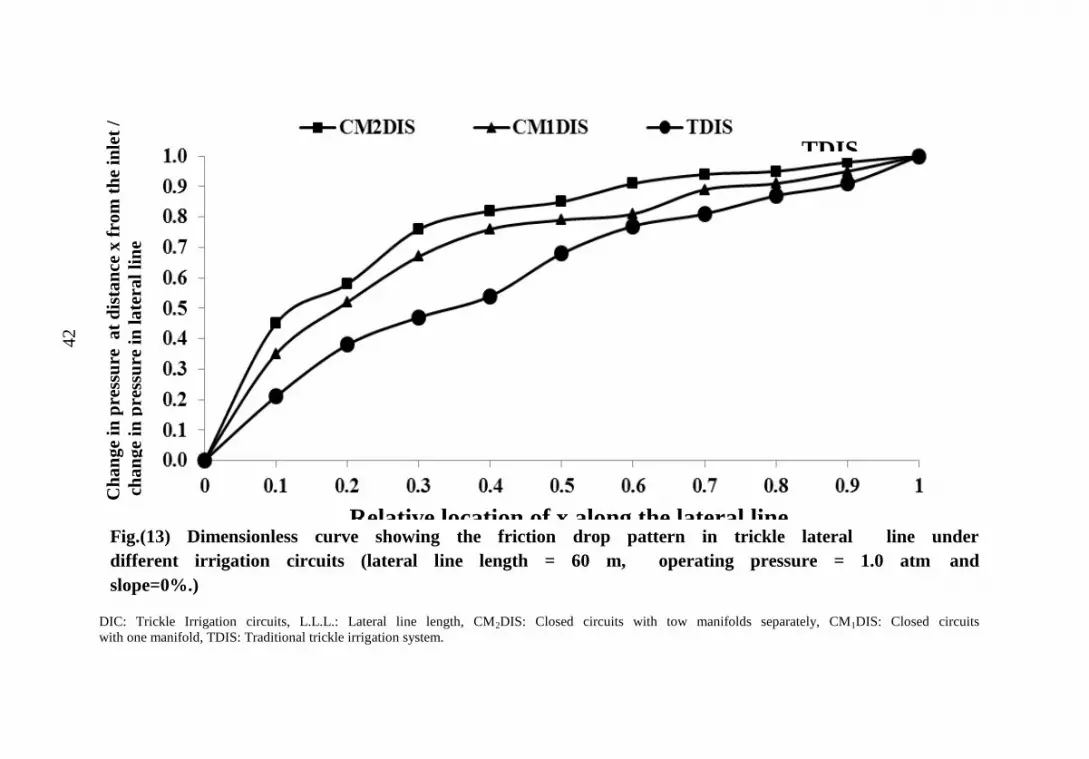
46

Fig.(13) Dimensionless curve showing the friction drop pattern in trickle lateral line under

different irrigation circuits (lateral line length = 60 m, operating pressure = 1.0 atm and

slope=0%.)



Ch

an

ge

in p

ress

ure

at

dis

tan

ce x

fro

m t

he

inle

t /

ch

an

ge

in p

ress

ure

in

late

ral

lin

e

Relative location of x along the lateral line

(x/L)

42

TDIS

37

Fig.(14) Dimensionless curve showing the friction drop pattern in trickle lateral line under different

irrigation circuits (lateral line length = 80 m, operating pressure = 1.0 atm and slope=0%.



Ch

an

ge

in p

ress

ure

at

dis

tan

ce x

fro

m t

he

inle

t /

chan

ge

in p

ress

ure

in

late

ral

lin

e

Relative location of x along the lateral line (x/L)

43

1

According to Table (8), pressure head variations given

acceptability results with all cases except interactions CM1DIS X

LLL3 and TDIS X LLL3.

Table (8) Effect of trickle irrigation closed-circuits (DIC) and

lateral line lengths (LLL) pressure head variation.

DIC L.L.L. Hmax

(m)

Hmin

(m)

H var

(%)

Acceptability by

ASAE Standard

2003

40 9.8 9.2 6.122 +++

CM2DIS 60 9.2 8.1 11.957 +++

80 9.1 7.8 14.286 +++

40 9.6 8.9 7.292 +++

CM1DIS 60 9.0 8.1 10.000 +++

80 8.8 6.6 25.000 ++

40 9.7 7.9 18.557 +++

TDIS 60 8.9 7.4 16.854 +++

80 8.1 3.8 53.086 ++

DIC: Trickle irrigation circuits, L.L.L.: Lateral line lengths, CM2DIS: Closed

circuits with tow manifolds separately, CM1DIS: Closed circuits with one

manifold, TDIS: Traditional trickle irrigation system, Hmax: The highest

pressure head, Hmin: The lowest pressure head, Hvar: Pressure head variation,

+++: acceptable and ++: unacceptable.

4.1.2. Friction loss:

Data given in Table (7) and plotted in Figs. (15 and 16)

indicated that the change of friction loss took an opposite trend to

that of H. Friction loss increased with distance from lateral inlet

reaching its maximum at 50 to 60 % of lateral length, then it

decreased again up to the lateral line end in the case of using

CM2DIS and CM1DIS. In other wards, the minimum values of

friction loss existed at both the inlets and the end of the lateral

lines. Reasons for this are due to the direct relation between

44

2

friction loss from one side and its length and discharge from the

other side.

According to the friction loss values, DIC could be put in

the following descending order: TDIS > CM1DIS > CM2DIS.

Differences in friction loss between any two DIC were significant

at the 1% level.

The ascending order: LLL1< LLL2< LLL3 illustrated the

mean effect of LLL on friction loss. Differences in friction loss

among LLL treatments were significant at the 1% level.

The effect of the DIC X LLL on friction loss was

significant at the 1% level. The maximum and minimum values

of friction loss were obtained in the interactions: TDIS X LLL3

and CM2DIS X LLL1, respectively. Fig. (15) Showing the

accepted and not accepted closed circuits by friction loss values.

Fig. (15). Effect of different closed circuits and lateral lengths

on friction loss.



manifold, TDIS: Traditional trickle irrigation system .

45

Lateral line length (m)

-------------------------------------------------------------------------------------------------

Above 20 % not accepted

CM2DIS CM1DIS TDIS

Fri

ctio

n l

oss

(m)

3

Fig.(16) Effect of different irrigation circuits designs on

friction loss along different lateral line lengths under

(operating pressure 1.0 atm and slope = 0%).



46

4

4.1.3. Flow velocity (FV):

Table (7) and Fig. (17) indicated the effect of DIC and

LLL on flow velocity. The reader can deduce that the change in

FV took the same trend of H, whereas, it was opposite to that of

friction loss. The explanation for this could be due to the effect of

both DIC on both H and friction loss. Also, increasing LLL

increased its discharge and decreased the amount of water

flowing along the lateral lines while, their cross section areas are

constant are other reasons.

According to the FV values, the DIC used could be put in

the following ascending order: TDIS < CM1DIS < CM2DIS.

Difference in FV between any two DIC was significant at the 1%

level. FV varied from 0.722 m/sec to 1.376 m/sec. i.e FV < 5

ft/sec and this is necessary to a avoid the effect of water hammer

in the main and sub-main lines, but in lateral line, it can cause silt

and clay precipitation problems.

Concerning the effect of LLL on FV, it is obvious that the

FV of LLL3 exceed that of LLL1, while that of LLL2 occupied

and intermediate position in between.

Differences in FV among LLL treatments were significant

at the 1% level. The effects of the DIC X LLL on FV were

significant at 1% level. The maximum and minimum flow

velocities were achieved in the interactions of: CM2DIS X LLL3

and TDIS X LLL2, respectively.

47

5

Fig. (17) Effect of different irrigation circuits designs on flow

velocity along different lateral line lengths under (operating

pressure 1.0 atm and slope=0%).



48

6

4.1.4. Velocity head:

Since velocity head is calculated from the following

equation: Velocity head = (flow velocity)2/ 2g i.e.≡

(m2 sec

-2) / 2(m sec

-2) ≡ m. It took the same trend of flow

velocity.

According to Table (7) and Fig. (18) Velocity head

values, DIC could be stated in the following ascending order:

TDIS < CM1DIS < CM2DIS. Differences in velocity head among

DIC were significant at the 1% level except that between

CM2DIS and CM1DIS.

Concerning the effect of LLL on velocity head, they can

be written in the follow ascending order: LLL1 < LLL2 < LLL3.

Differences in velocity head among LLL treatments were

significant at the 1% level without exceptions.

The effects of the DIC X LLL on velocity head were

significant at the 1% level except some cases i.e. CM2DIS X

LLL2, CM1DIS X LLL1and TDIS X LLL3.

The maximum and minimum values of velocity head were

found in the following interactions: CM2DIS X LLL3 and TDIS X

LLL1, respectively.

49

7

Fig. (18) Effect of different closed circuits designs on velocity

head along different lateral line lengths under (operating

pressure 1.0 atm and slope=0%)



50

8

4.1.5. Emitter discharge and variations:

Tables (9; 10) and Fig. (19) showed the effect of DIC and LLL

on emitter discharge variation (qvar) and emitter discharge (qd).

According to emitter discharge variation values, all cases were

acceptability except TDIS with LLL3. According to emitter discharge

values, DIC used could be stated in the following ascending order: TDIS

< CM1DIS < CM2DIS. Difference in qd between any two DIC was

significant at the 1 % level except that between CM2DIS and CM1DIS.

This may be due to the effect of DIC on both pressure head and friction

loss. The obtained data revealed no significant difference at the 1% in qd

among the LLL used. Reason for this is due to stability of both lateral

lines Ø (16 mm) and their slope. The effect of DIC X LLL ended

with significant differences in qd at the 1% level in most cases. The

maximum value of qd (4.18 Lh-1

) and the minimum one (2.6 Lh-1

) were

achieved in the following interactions: CM2DIS X LLL1 and TDIS X

LLL3, respectively.

Table (9) Effect of DIC design and LLL on emitter qvar

percent.

DIC L.L.L. qmax

(Lh-1

)

qmin

(Lh-1

)

q var

(%)

Acceptability,

ASAE 2003

40 4.23 4.1 3.07 +++

CM2DIS 60 3.77 3.65 3.18 +++

80 3.76 3.66 2.66 +++

40 4.11 4.04 1.70 +++

CM1DIS 60 3.65 3.45 5.48 +++

80 3.63 3.49 3.86 +++

40 3.49 2.8 19.77 ++

TDIS 60 2.92 2.37 18.84 ++

80 2.55 1.79 29.80 +



manifold, TDIS: Traditional trickle irrigation system, qmax: The highest

discharge, qmin: The lowest discharge, qvar: emitter discharge variation, +++:

excellent, ++: acceptable and +: unacceptable.

51

9

Table (10) Effect of DIC and LLL on both emitters; lateral discharge and uniformity under

(operating pressure = 1 atm and slope = 0%).

DIC L.L.L. Emitter

discharge,

(Lh-1

)

Lateral discharge,

(Lh-1

)

Uniformity

coefficient %

Coefficient of

variation (CV)

CV acceptability

by ASAE 1996

40 4.18 a 555.9 fe 97.74 a 0.081 g +++

CM2DIS 60 3.72 c 744.0 c 95.14 cb 0.063 ig +++

80 3.71 dc 990.0 a 92.03 d 0.122 fe ++

40 4.07 ba 541.0 g 95.73 b 0.071 hg +++

CM1DIS 60 3.51 fe 702.0 dc 89.45 ef 0.162 ec ++

80 3.59 e 958.0 ba 83.25 h 0.231 b ++

40 3.21 g 426.0 i 88.27 f 0.183 de ++

TDIS 60 2.60 h 520.0 h 84.73 g 0.221 cb ++

80 2.16 i 576.7 e 80.53 i 0.280 a +

LSD 0.01 X

0.18 80.33 1.18 0.042

Means CM2DIS 3.87 a 762.35 a 94.97 a 0.089 c +++

CM1DI 3.72 ba 732.71 ba 89.47 b 0.155 b ++

TDIS 2.66 c 507.22 c 84.51 cb 0.228 a ++

LSD 0.01 0.44 205.75 5.19 0.027

Means 40 3.82 a 507.78 cb 93.91 a 0.112 c +++

60 3.28 ba 655.64 b 89.77 ba 0.149 b ++

80 3.15 cba 838.87 a 85.27 cb 0.211 a ++

LSD 0.01 0.77 177.05 6.91 0.028

DIC: Trickle irrigation circuits, L.L.L.: Lateral line lengths, CM2DIS: Closed circuits with tow manifolds separately, CM1DIS:

Closed circuits with one manifold, TDIS: Traditional trickle irrigation system,+++= Excellent, ++=Good, +=Fair, and LSD 0.01:

less significant different at 1% Significant level.

52

10

Fig.(19) Effect of different irrigation circuits designs on

emitter discharge along different lateral line lengths under

(operating pressure 1.0 atm and slope = 0%).



53

11

4.1.6. Lateral line discharge (Ql):

Data on hand Table (8) and Fig. (20) illustrated the

effect of DIC and LLL on Ql. Regardless of LLL the effect of

DIC on Ql could be summarized in the following ascending

order: TDIS < CM1DIS <CM2DIS.

The following descending order: LLL3 < LLL2 < LLL1

showed that the differences in Ql among LLL were significant

at the 1 % level except between LLL1 and LLL2. Although LLL

has no significant effect on qd, the effect of LLL on Ql was a

significant one. Reason for this is due to increasing emitter

number per lateral line with increasing it length. i.e. emitter

numbers were 133, 200 and 267 for the LLL 40, 60,80 m,

respectively.

The effect of the interaction DIC X LLL on Ql was

significant at the the 1 % level with few exceptions. The

maximum values of Ql (990 Lh-1

) and the minimum one (426

Lh-1

) were achieved in the interactions: CM2DIS X LLL3 and

TDIS X LLL1, respectively.

54

12

Fig. (20) Effect of different irrigation circuits designs on lateral discharge for different lateral

line lengths under (operating pressure 1.0 atm and slope 0%).

LLL1: Lateral line length = 40m, LLL2: Lateral line length = 60m, LLL3: Lateral line length = 80m CM2DIS: Closed circuits with tow

manifolds separately, CM1DIS: Closed circuits with one manifold, TDIS: Traditional trickle irrigation system.

55

13

4.1.7. Uniformity coefficient (UC):

Table (8) and Fig. (21) exhibited the role of both DIC

and LLL on UC.

The mean effect of DIC on UC could be put in the

follow ascending order: TDIS ≤ CM1DIS < CM2DIS.

Differences in UC among DIC used were significant at the 1 %

level except that between CM2DIS and TDIS.

Concerning the mean effect of LLL on UC regardless of

DIC used can be dictated in the following ascending order:

LLL3 ≤ LLL2 ≤ LLL1. Differences in UC between LLL was

significant at the 1 % level only between LLL1and LLL3.

It is worthy to mention the values of UC took an

opposite trend to that of Ql. this is mainly due increasing both

Ql and LLL which affected pressure head negatively and

friction loss positively.

The effect of the interaction: DIC X LLL on UC was

significant at 1 % level with one exception i.e. between the

interactions: CM2DIS X LLL2 and CM1DIS X LLL2. The

maximum value of UC (97.74 %) and the minimum one (80.53)

can be seen in the interaction: CM2DIS X LLL1 and TDIS X

LLL3, respectively.

The acceptable values of CV were all cases except

interactions below line of acceptability as showing Fig. (21)

(CM1DIS X LLL3), (TDIS X LLL2) and (TDIS X LLL3).

56

14

Fig. (21) Effect of different irrigation circuits designs on uniformity coefficient (UC) for

different lateral line lengths under (operating pressure 1.0 atm and slope=0%).


manifolds separately, CM1DIS: Closed circuits with one manifold, TDIS: Traditional trickle irrigation system

57

--------------------------------------------------------------------------------------------------------------- --------------------------

Accepted

Values line

Above

85 %

15

4-1-8. Coefficient of variation for emitter discharge.

Data on the effect of DIC and LLL on CV are tabulated in

Table (8) and plotted in Fig. (22). It is clear that the trend of CV

values was similar to that of Ql, whereas it was opposite to that of UC.

The main positive effect of DIC on CV despite of LLL could be

arranged in the following ascending order: TDIS < CM1DIS <

CM2DIS. Differences in CV among DIC were significant at the 1%

level. Data on hand indicated that the degree of CV acceptability

according to ASAE (1996) was excellent and good using CM2DIS and

both CM1DIS and TDIS, respectively.

Fig. (22) and Table (8) illustrated the effect of LLL on CV

despite of DIC used. The effect of LLL on CV could be summarized in

the following ascending order LLL3< LLL2< LLL1. The difference

between any two LLL treatments was significant at the 1 % level. It is

clear from data on hand that CV acceptability was excellent and good

in LLL1 and both LLL2 and LLL3, respectively.

One can deduce the effect of the interaction of DIC X LLL on

CV from Table (8) and Fig. (22). The differences in CV values were

insignificant at the 1 % level among any of the following interactions:

(CM2DIS X LLL1, CM2DIS X LLL2; CM1DIS X LLL1), CM2DIS X

LLL3, CM1DIS X LLL2; TDIS X LLL1) and (CM1DIS X LLL2; TDIS

X LLL3).

The highest value (0.28) and the lowest one (0.063) of CV were

obtained in the interactions: (TDIS X LLL3), and (CM2DIS X LLL2),

respectively.

Finally, the degrees of CV acceptability of DIC X LLL were

excellent, fair and good in the interaction: (CM2DIS X LLL1, CM2DIS

58

16

X LLL2; CM1DIS X LLL1), (TDIS X LLL3) and in all the other

interactions), respectively.

It worthies to state that through DIC and LLL trickle

irrigation system could be managed towards improving all the

hydraulic characteristics under investigation. This would cause

an increase in uniformity distribution of both water and

fertilizers, and subsequently in plant growth, yield, water use

efficiency, fertilizer use efficiency and in cost analysis.

The acceptable values of CV were all cases except

interactions (CM1DIS X LLL3), (TDIS X LLL2) and (TDIS X

LLL3) above line of acceptability as showing Fig. (22). This

due to the difference in pressure head in different closed circuits

and along different lateral line lengths therefore reflected on

velocity, head losses and CV values of emitter discharge.

59

17

Fig. (22) Effect of different irrigation circuits designs and lateral line lengths on coefficient of

variation (CV) for under (operating pressure 1.0 atm and slope = 0%)


manifolds separately, CM1DIS: Closed circuits with one manifold; TDIS: Traditional trickle irrigation system.

60

60

-----------------------------------------------------------------------------------------------------------------------------------------

Accepted

Values line

Below

20 %

18

4.1.9 Comparing the practical data of head loss along the

lateral line in the laboratory with those calculated using

Hydro-Calc simulation program.

The discharge rates and pressures of trickle pressure

head were measured under field conditions at three locations

along the lateral lines for CM2DIS, CM1DIS, and TDIS using

three different LLL (LLL1 = 40m, LLL2 = 60m and LLL3 =

80m). Empirical estimates were used to validate the trickle

simulation program (Hydro-Calc Simulation program copyright

2009 developed by NETAFIM, USA). Hydro-Calc, is a

computer simulation program used for planning and design of

trickle or sprinkler irrigation systems. Modification of trickle

irrigation closed circuit (DIC) lateral lines lengths (LLL)

depends mainly on hydraulic equations such as, Hazen-

William’s equations, Pernolli’s equations, etc. The data inputs

provided to Hydro-Calc were shown in Table (9). The

empirical data depended on the laboratory measurements of

both emitter pressure and discharge, as well as the uniformity of

water distribution.

The predicted outputs of Hydro-Calc simulation

program (exponent (X), head loss (m) and velocity (m sec-1

))

were shown in Table (10) and Figs. (23, 24, and 25). The

differences in exponent (x) values of emitter built-in attributed

to the different closed circuits and different lateral line lengths

therefore the pressure has been affected and the difference

pressures effects on (x) values.

61

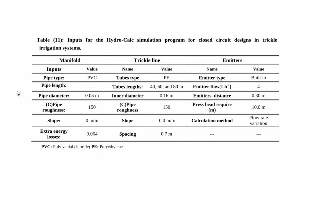
19

Table (11): Inputs for the Hydro-Calc simulation program for closed circuit designs in trickle

irrigation systems.

Manifold Trickle line Emitters

Inputs Value Name Value Name Value

Pipe type: PVC Tubes type PE Emitter type Built in

Pipe length: ----- Tubes lengths: 40, 60, and 80 m Emitter flow(Lh-1

) 4

Pipe diameter: 0.05 m Inner diameter 0.16 m Emitters distance 0.30 m

(C)Pipe

roughness: 150

(C)Pipe

roughness 150

Press head require

(m) 10.0 m

Slope: 0 m/m Slope 0.0 m/m Calculation method Flow rate

variation

Extra energy

losses: 0.064 Spacing 0.7 m --- ---

PVC: Poly venial chloride; PE: Polyethylene.

62

20

Table (12): Predicted exponent (x), Head loss (m) and velocity (m sec-1

) by the Hydro-Calc

simulation program for closed circuits trickle irrigation design.

L.L.L.,

(m)

DIC

CM2DIS CM1DIS TDIS

Exponent

(x)

Head loss

(m)

Velocity

(m sec-1)

Exponent

(x)

Head loss

(m)

Velocity

(m sec-1)

Exponent

(x)

Head loss

(m)

Velocity

(m sec-1)

40 0.72 0.53 1.40 0.69 0.82 1.35 0.58 1.12 0.87

60 0.65 1.27 1.08 0.61 1.69 0.98 0.55 2.19 0.71

80 0.58 1.69 0.79 0.52 2.96 0.75 0.53 3.98 0.62

DIC: Trickle irrigation circuits, L.L.L.: Lateral line lengths, CM2DIS: Closed circuits with tow manifolds separately,

CM1DIS: Closed circuits with one manifold, TDIS: Traditional trickle irrigation system

63

21

Table (13): Effects of different DIC and different LLL on hydraulic parameters under (operating

pressure 1.0 atm and slope = 0%). (Calculated by Hydro-Calc. simulation program).

Hydraulic parameters CM2DIS CM1DIS TDIS

LLL1 LLL2 LLL3 LLL1 LLL2 LLL3 LLL1 LLL2 LLL3

No. of emitters 133 200 267 133 200 267 133 200 267

Emitter (q) (lH) 4.09 3.63 3.56 4.02 3.57 3.51 3.16 2.56 2.04

Total (Q) (lH) 544 726 950 535 714 937 420 512 545

Avg. flow velocity m/sec 0.86 1.54 1.88 0.91 1.73 1.92 0.94 1.62 1.97

Reynolds number 3238 3001 3062 3859 3753 3810 3234 3489 3612

Flow type Turbulent

Critical velocitym/s 0.82 1.48 2.83 0.87 1.68 1.85 0.89 1.58 1.93

f =ε /d 0.23

Hf (m) 0.53 1.07 1.75 0.83 1.09 2.57 1.34 2.31 4.28

f = ε/d = Roughens Coefficient, Rn > 3000 = Turblent flow, Rn < 3000 = Laminar flow (Hathoot, et al, 1993). LLL1: Lateral

line length = 40m, LLL2: Lateral line length = 60m, LLL3: Lateral line length = 80m CM2DIS: Closed circuits with tow manifolds

separately, CM1DIS: Closed circuits with one manifold; TDIS: Traditional trickle irrigation system.

64

68

22

The predicted head loss analysis along the lateral lines had been

calculated by Hydro-Calc simulation program for irrigation closed

circuits of trickle irrigation systems CM2DIS and CM1DIS compared

with TDIS under different LLL of LLL1, LLL2, and LLL3. The predicted

and measured head losses values were tabulated in Tables (2, 3 and 4) in

Annex (1). Figs. (23, 24 and 25) showed the relationships among the

predicted and measured head losses as well as regressions and

correlations under CM2DIS, CM1DIS, and TDIS methods.

Clearly the irrigation methods under study that used LLL1 and

LLL3 could be ranked in the ascending order by both the predicted and

measured head losses CM2DIS<CM1DIS<TDIS. Under LLL2, the

irrigation circuits could be ranked in the following ascending order

CM1DIS<CM2DIS<TDIS. The variation in rankings may be attributed to

the different numbers of emitters or how many emitters were built-in

with every lateral line length. The regression (R²) had been obtained to

compare the significance of the predicted and measured head loss along

the lateral lines of the three closed circuits designs. The deviations were

simple between all predicted and measured values exception the

interaction TDIS X LLL3.

Generally, the values of regression analysis between predicted

and measured values were significant at the 1 % level, under different

DIC and LLL (experimental conditions) were used.

65

23

Fig. (23). The relationship between different lateral line

lengths (40, 60 and 80 m) and both the predicted and

measured head losses when pressuer head 1.0

atm.under CM2DIS design.

Hea

d l

oss

e (m

)

Hea

d l

oss

e (m

)

Hea

d l

oss

e (m

)


66

24

Fig. (24).The relationship between different lateral line lengths

(40, 60 and 80 m) and both the predicted and measured

head losses when operatingpressure 1.0 atm with the

CM1DIS design.

Hea

d l

oss

e (m

)

Hea

d l

oss

e (m

)

Hea

d l

oss

e (m

)


67

25

Fig. (25).The relationship between different lateral line lengths (40,

60 and 80 m) and both the predicted and measured head

losses whenoperating pressure head 1.0atm with the TDIS

design.

Hea

d l

oss

e (m

)

Hea

d l

oss

e (m

)

Hea

d l

oss

e (m

)


68

26

4.4. Effect of DIC and LLL on vegetative growth and yield

parameters of corn plant.

Table (14) showed the main one of trickle irrigation

circuits (DIC) and sub-main one of the lateral line length

(LLL) on some vegetative growth and yield parameters of

corn. Measured parameters were: average leaf area (cm2),

plant height (cm), leaf length (cm), number of leaves, grain

yield (ton/fed) and stover yield (ton/fed).

4-4-1. Leaf area (LA) (cm2):

Table (14) illustrated the effect of DIC and LLL on

LA (cm2). According to LA values, DIC could be ranked in

the following descending order: CM2DIS > CM1DIS > TDIS.

Differences in LA among DIC were significant at the 1 %

level. The effect of LLL on LA could be put in the following

descending order: LLL1>LLL2>LLL3. Differences in LA

values were significant at the 1% level. The effect of

interactions: DIC X LLL on LA were significant at 1% level.

The maximum value of LA (499.73 cm2) and the minimum

one (478.31 cm2) were obtained in the interactions: CM2DIS

X LLL1 and TDIS X LLL3, respectively.

4-4-2. Plant height (HP)(cm):

Data in Table (14) indicated the effect of DIC and

LLL on HP (cm). Due to the HP values, DIC and LLL could

be Written in the following descending order: CM2DIS >

CM1DIS > TDIS. On the other hand, LLL treatments could be

sorted in the following descending order: LLL1> LLL2> LLL3.

Differences in HP values among DIC and /or LLL treatments

were significant at 1 % level except that between CM2DIS and

CM1DIS.

69

27

The interactions: DIC X LLL affected HP significantly

at the 1 % level with the exception of the interactions:

(CM2DIS X LLL3, CM1DIS X LLL2, CM1DIS X LLL3 and

TDIS X LLL3). The maximum (193.78 cm) and minimum

(191.45 cm) values of HP were achieved in the following

interactions: (CM2DIS X LLL1and TDIS X LLL3),

respectively.

4-4-3.Leaf length (LL):

Table (14) showed the effect of both DIC and LLL on LL in

cm. Regarding the values of LL, DIC and LLL treatments could be

mentioned in the following descending orders: CM1DIS > CM2DIS >

TDIS and LLL1 ≥ LLL2 > LLL3, respectively. Differences in LL

among LLL1, LLL2 and LLL3 treatments were significant at the 1%

level.

Data on hand indicated that the effects of the interactions:

DICXLLL were significant at the 1% level. The maximum value

(68.15 cm) and the minimum one (64.26 cm) were recorded in the

interactions: CM2DIS X LLL1 and TDISXLLL3, respectively.

4-4-4.Number of leaves per plant (LN plant-1

):

The effect of DIC and LLL on LN plant-1

could be

deduced from Table (12).

According to the values of LN plant-1

, DIC and LLL

on LN plant-1

, it could be stated in the following descending

order: CM2DIS > CM1DIS > TDIS and LLL1 > LLL2 > LLL3

i.e. neither DIC nor LLL treatments had significant effects on

LNplant-1

at the 1 % level. Differences in LN per plant

between means of the two factors studied were significant at

the 1 % level.

7

0

70

28

The obtained data, illustrated that the interactions of

DICXLLL treatments had significant effects on LN plant-1

at

the 1% level. The maximum value of LN plant-1

(15.45) and

the minimum one (14.55) was found in the interactions:

CM2DIS X LLL1; TDIS X LLL3, respectively.

The superiority of the studied growth parameters under

(CM2DIS; CM1DIS relative to TDIS) and (LLL1; LLL2

relative to LLL3) can be noticed this superiority was due to

improving both water and fertilizers distribution uniformity.

71

29

Table (14): Effect of trickle irrigation circuits and lateral lines lengths on corn plants growth and yield.

DIC

LLL Growth and Yield Characters at Harvest (average)

(m)

Leaf area (cm2)

Plant Leaf length

(cm)

No. of leaves

per plant

Yield (ton/fed)

height (cm) Grain Stover

CM2DIS

40 499.73a 193.78a 68.51a 15.45a 5.41a 3.52a

60 491.53d 192.21f 66.85c 15.32b 5.14c 3.47d

80 488.37e 192.75dc 65.25g 15.15c 5.05ed 3.42f

40 498.43b 193.30b 67.21b 14.97d 5.30b 3.50ba

60 485.33g 192.85c 66.34e 14.78f 5.05fe 3.44e

CM1DIS 80 479.83h 191.53h 64.42h 14.66h 4.99g 3.40h

TDIS

40 496.35c 192.66e 66.58d 14.86e 5.05d 3.48cb

60 486.78f 191.83g 65.73f 14.72g 4.64h 3.41g

80 478.31i 191.45ih 64.26i 14.55i 4.38i 3.40ih

(1) X (2) LSD 0.01 1.27 0.11 0.14 0.09 0.03 0.02

(1) Means CM2DIS 492.77a 192.75a 66.87b 15.31a 5.26a 3.47a

CM1DIS 488.29b 192.72ba 66.99a 14.80ba 5.11b 3.45b

TDIS 487.15c 191.98c 65.52c 14.71ca 4.69c 3.43c

LSD 0.01 4.18 0.12 0.08 1.77 0.07 0.02

(2) Means 40 498.17a 193.25a 67.43a 15.09a 5.26a 3.50a

60 487.88b 192.30b 66.31ba 14.94ba 4.94b 3.44b

80 482.17c 191.91c 64.64c 14.79ca 4.81c 3.41c

LSD 0.01 3.72 0.26 2.77 1.81 0.04 0.02

DIC: Trickle irrigation circuits, L.L.L.: Lateral line lengths, CM2DIS: Closed circuits with tow manifolds separated,

CM1DIS: Closed circuits with one manifold, TDIS: Traditional trickle irrigation system

72

30

4-4-5. Grain yield (GY):

Data of Table (12) indicated the effect of DIC and LLL

treatments on corn GY (ton fed-1

). Due to the values of GY the

treatments used could be arranged in the following ascending

orders: TDIS < CM1DIS < CM2DIS and LLL3< LLL2< LLL1.

Differences in GY among DIC and/or LLL treatments were

significant at the 1% level.

Concerning the effects of the interaction: DIC X LLL

treatments on GY, they were significant at the 1% level except

that between any two interactions of: CM2DIS X LLL3, CM1DIS

X LLL2 and TDIS X LLL1. The maximum and the minimum GY

(5.14; 4.38 ton fed-1

) were achieved in the interactions: CM2DIS

X LLL1 and TDIS X LLL3, respectively.

We can notice that corn GY took the same trend of the

growth parameters and this finding could be attributed to the

close correlation between vegetative growth from one side and

GY from the other one.

4-4-6- Stover yield (SY):

The effect of both DIC and LLL treatments used on SY

(ton fed-1

) could be seen in Table (12). one can notice that the

change in SY took the same trend of the other growth parameters

under investigation.

Concerning the values of SY, the DIC and LLL could be

ranked in following descending orders: CM2DIS > CM1DIS >

TDIS and LLL1> LLL2> LLL3, respectively.

The differences in SY among both DIC and LLL

treatments were significant at the 1%.

73

31

It is obvious that the effects of the interactions: DIC X

LLL treatments on SY were significant at the 1% level except

that between the interactions: (CM1DIS X LLL3; TDIS X LLL2)

and (CM1DIS X LLL3, TDIS X LLL2; TDIS X LLL3).

In conclusion, the closed trickle irrigation circuits

(CM1DIS; CM1DIS) and decreasing LLL improved some

hydraulic characteristics of the irrigation system i.e. pressure

head, friction loss, flow velocity, velocity head,, uniformity,

coefficient of variation…ex. relative to TDIS. This of course

improved the distribution of both water and fertilizers along the

lateral lines and subsequently all the growth parameters under

study.

4-4-7.Grain and Stover water use efficiency (WUEg and

WUEs).

Table (15) indicated the effect of both, DIC and LLL

treatments used on WUEg and WUEs. One could deduce that the

changes in WUEg and WUEs took the same trend of the vegetative

growth parameters under investigation i.e. leaf area, plant height,

leaf length and number of leaves per plant. This could be due to

the positive effect of DIC and LLL treatments on the vegetative

growth parameters mentioned above.

According to WUEg and WUEs values, DIC could be put

in the following descending orders: CM2DIS > CM1DIS > TDIS

and CM2DIS > CM1DIS > TDIS, respectively. Differences in

WUEg only among DIC were significant at the 1% level.

In respect to the WUEg and WUEs values, the LLL could

be illustrated in the following descending orders:

LLL1>LLL2>LLL3 and LLL1 ≥ LLL2 ≥ LLL3, respectively.

Differences in WUEg among LLL treatments were significant at

the 1% level, except that between LLL2 and LLL3. On the other

74

32

hand, difference in WUEs was significant at the 1% level only

between LLL1 and LLL3.

The effect of the interaction: DIC X LLL on WUEg were

significant at the 1% level, except those among the interactions:

CM2DIS X LLL3, CM1DIS X LLL2 and TDIS X LLL1. The effect

of interaction: DIC X LLL on WUEs were not significant at the

1% level in most cases. The highest of WUEg and WUEs (1.33;

0.87 ton fed-1

) and the lowest one (1.14; 0.84 ton fed-1

) were

obtained in the interactions: CM2DIS X LLL1 and TDIS X LLL2

or LLL3, respectively.

Table (15) Effect of different irrigation circuits designs and

different lateral lines lengths on WUE.

DIC LLL (m)

Applied

water

(m3/fed)

Grain Stover

yield

(kg/fed)

WUEg

(kg/m3)

yield

(kg/fed)

WUEs

(kg/m3)

40

4060.1

4

5411.8a 1.33a 3522.7a 0.87a

CM2DIS 60 5139.0c 1.27c 3466.6d 0.85dab

80 5049.7ed 1.24ed 3416.7f 0.84fb

40 5302.0b 1.31ba 3496.6a 0.86ba

CM1DIS 60 5046.5fe 1.24d 3443.4e 0.85eab

80 4986.1g 1.23g 3400.1h 0.84gb

40 5052.3d 1.24f 3475.4c 0.86ca

TDIS 60 4634.3h 1.14i 3404.2g 0.84hb

80 4380.5i 1.18h 3394.5i 0.84ib

1 X 2 LSD 0.01 78.6 0.02 17.62 0.02

Means (1) CM2DIS 5200.2a 1.28a 3468.6a 0.85a

CM1DIS

5111.5b 1.26b 3446.7b 0.85ba

TDIS 4689.0c 1.19c 3424.7c 0.84cab

LSD 0.01 64.3 0.01 9.7 0.03

Means (2) 40 5255.4a 1.29a 3489.2a 0.86a

60

4939.9b 1.22b 3438.1b 0.85ba

80 4805.5c 1.22c 3403.8c 0.84cba

LSD 0.01 89.4 0.03 25.4 0.02

DIC: Trickle irrigation circuits, L.L.L.: Lateral line lengths, LLL1: Lateral line length = 40m,

LLL2: Lateral line length = 60m, LLL3: Lateral line length = 80m CM2DIS: Closed circuits with tow

manifolds separately, CM1DIS: Closed circuits with one manifold; TDIS: Traditional trickle irrigation

system.

7

5

75

33

4-4-8. Fertilizers use efficiency (FUE):

Table (16) showed the effect DIC and LLL treatments on

(N, P2O5; K2O) fertilizers use efficiency (FUEN, FUEP2O5;

FUEK2O).

According to the FUE values of the three fertilizers used,

the DIC and LLL treatments used could be ranked in the

following ascending orders, TDIS < CM1DIS < CM2DIS and

LLL3< LLL2< LLL1. Differences in FUE among DIC between

any two DIC treatments and /or LLL ones were significant at the

1% level except that between (CM2DIS, CM1DIS) and (LLL2;

LLL3) in the case of (FUEN). Whereas under the effect LLL, there

were significant differences at 1 % level in FUE among LLL

except that between LLL2 and LLL3 in NUEN.

The effects of the interactions: DIC X LLL treatments on

FUE were significant at the 1% level among some interactions

and not among the others. The highest values of FUE N, FUE P2O5

and FUEK2O (89.5, 180.5; 188.1 kg yield.kg fertilizer-1

) and the

lowest ones (42.5, 146.1; 152.2 kg yield.kg fertilizer-1

) were

achieved in the interactions: CM2DIS X LLL1 and TDIS X LLL3,

respectively. These data are supported by Baligar and Bennett

(1986).

The obtained results indicated that FUE took the same

trend of vegetative growth parameters, yield and WUE. This

finding may be attributed to the direct relation between WUE and

FUE found by Tayel et al, (2006).

76

34

Table (16): Effect of different trickle irrigation circuits designs and lateral lines lengths on FUE.

DIC LLL(m)

Applied fertilizers

(kg/fed) Grain yield

(kg /fed)

FUE

(kg yield / kg fertilizer)

N P2O5 K2O

N U E P U E K U E

CM2DIS 40

60.48 71.4 68.52

5411.8a 89.5a 180.5a 188.1a

60 5139.0c 85.0c 171.4c 178.6c

80 5049.7ed 83.5ec 168.4e 175.5ed

CM1DIS 40 5302.0b 87.7ba 176.8b 184.2ba

60 5046.5fe 83.4fc 168.3f 175.4fd

80 4986.1g 82.4gd 166.3g 173.3gd

TDIS

40 5052.3d 83.5dc 168.5d 175.6d

60 4634.3h 76.6i 154.5h 161.0h

80 4380.5i 72.4h 146.1i 152.2i

X LSD 0.01

78.6 3.2 3.5 4.1

Means CM2DIS

5200.2a 86.0a 173.4a 180.7a

CM1DIS

5111.5b 84.5ba 170.5b 177.6b

TDIS

4689.0c 77.5c 156.4c 162.9c

LSD 0.01

64.3 1.6 1.8 2.2

Means 40

5255.4a 86.9a 175.2a 182.6a

60

4939.9b 81.7b 164.7b 171.7b

80

4805.5c 79.5cb 160.2c 167.0c

LSD 0.01

89.4 3.8 4.4 2.7

DIC; Trickle irrigation circuits, LLL: Lateral line lengths, FUE = Fertilizers use efficiency, NUE = Nitrogen use efficiency, PUE = HosHorous use

efficiency, KUE = Potassium use efficiency, LLL1: Lateral line length = 40m, LLL2: Lateral line length = 60m, LLL3: Lateral line length = 80m CM2DIS:

Closed circuits with tow manifolds separated, CM1DIS: Closed circuits with one manifold; TDIS: Traditional trickle irrigation system.

77

4-5. Effect of (DIC) and (LLL) on costs analysis of corn production:

Total costs of agricultural operations are major capital

inputs for most farms. The capital and annual costs (fixed and

operating ons) of different DIC: CM2DIS (with two manifolds),

CM1DIS (with one manifold) and traditional trickle irrigation

(TDIS) and LLL: (LLL1 = 40m, LLL2 = 60m; LLL3 = 80m) on

costs analysis of corn production (total cost, total revenue and

both physical and money income per unit used of irrigation water

were given in Tables (15 and 16) and plotted in Figs (31, 32 and

33).

Data on hand indicated that the studied parameters

differed according to DIC and LLL used. Table (17) showed that

the capital costs (LE fed-1

) ranged from (5008-5658), (5032-

5632) and from (4962-5562) according to LLL under CM2DIS,

CM1DIS and TDIS, respectively. It was obvious that the capital

costs increased with decreasing LLL. This may due to the extra

length of tubes used as manifolds and valves.

Relative to the total costs, the fixed ons accounted to

(40.35, 39.03; 37.46 %), (40.12, 38.83; 37.45 %) and (39.7,

35.69; 37.0 %) under CM2DIS, CM1DIS, TDIS, LLL1, LLL2 and

LLL3, respectively. On the other hand, the operation costs

reached: (10.04, 10.26; 10.53 %), (10.27, 10.5; 10.73 %) and

(10.58, 11.29; 11.06 %) of the total ones in the same sequency

mentioned before.

Table (17) illustrated grain yield, stover yield, the net

profit and both the physical and money income from the unit of

irrigation water used. The obtained values of these parameters

were: (5412, 5139; 5049 kg fed-1

), (5302, 5046; 4986 kg fed-1

),

(5052, 4634; 4381 kg fed-1

), (234, 222; 218 kg fed-1

), (229, 218;

216 kg fed-1

) and (218, 200; 189 kg fed-1), (2.20, 2.12; 2.08

kg/m3), (2.17, 2.09; 2.06 kg/m

3), (2.10, 1.98; 1.90 kg/m

3), (0.43,

78

0.41; 0.40 LE/m3), (0.42, 0.40; 0.39 LE/m

3) and (0.21, 0.19; 0.18

LE/m3) in the same sequence under (CM2DIS, CM1DIS; TDIS)

and (LLL1, LLL2; LLL3), respectively.

Table (18) stated the effect of both DIC and LLL used on

the total costs (LE fed-1

season-1

), total revenue (LE fed-1

season-

1), physical income (kg/m

3) and the money income (LE/m

3).

Concerning the effect of DIC on the parameters under

consideration, the DIC used could put in the following

descending orders: (CM2DIS = CM1DIS > TDIS), (CM2DIS >

CM1DIS > TDIS), (CM2DIS = CM1DIS > TDIS), (CM2DIS >

CM1DIS > TDIS), in the same sequency, respectively. In other

wards, differences in total costs and physical income between

CM2DIS and CM1DIS from one side and TDIS system from the

other side were significant at the 1 % level, whereas, the

differences in both the total revenue and money income from unit

of irrigation water used among DIC were significant at the 1%

level.

In the case of the effect of LLL on all the studied

parameters LLL could be ranked in the following ascending

order: LLL1 < LLL2 < LLL3 except the physical income, whereas

the order took the trend: LLL1 < LLL2 < LLL3. Differences in

data on hand among LLL were significant at the 1% level except

that between LLL2 and LLL3 in the case of the physical income.

The effects of the interaction DIC x LLL were given in

Table (18). The maximum values and the minimum ones of the

total costs, total revenue, the physical income and the money

income from irrigation water unit used were achieved in the

following interactions: (CM2DIS X LLL1; TDIS X LLL2),

(CM2DIS X LLL1; TDIS X LLL3), (CM2DIS X LLL1; TDIS X

LLL3) and (CM2DIS X LLL1; TDIS X LLL3), respectively.

The data obtained could be explained on the basis that

7

9

79

DIC and LLL effects on the investigated parameters were through

their effect on some hydraulic characteristics i.e. emitter

discharge, lateral discharge, pressure head, friction loss, flow

velocity, velocity head, uniformity coefficient and coefficient of

variation. The positive effect of CM2DIS and CM1DIS and the

short LLL on these parameter led to better distribution of both

water and fertilizers along the lateral lines. This was positively

reflected on corn yield per feddan and subsequently on both the

physical and the money income from the unit of irrigation water

used. In the same time, the effect of DIC and LLL on the

parameters under consideration through the fixed and operating

costs was quite nil.

80

Table (17) Agricultural Cost analysis of corn production under different DIC and LLL (LE fed-1

season-1

)

Cost items CM2DIS CM1DIS TDIS

40 60 80 40 60 80 40 60 80

Capital cost (LE/fed) 5658 5358 5008 5632 5332 5032 5562 5262 4962

Fixed costs (LE/fed/season)

1- Depreciation 396 375 351 394 373 352 389 368 347

2- Interest 226 214 200 225 213 201 222 138 198

3- Taxes and insurance 85 80 75 84 80 75 83 79 74

Sub-total 707 669 626 703 666 628 694 585 619

Operating costs (LE/fed/season)

1- Electricity for pump motor 76 80 85

2- Maintenance and Repairing 100 100 100

Sub-total 176 180 185

Total annual irrigation cost (LE/fed/season) 883 845 802 883 846 808 879 770 804

Total agricultural Costs 869 869 869

Total costs (LE/fed/season) 1752 1714 1671 1752 1715 1677 1748 1639 1673

Yield Grain, (kg/fed) 5412 5139 5049 5302 5046 4986 5052 4634 4381

Stover,(kg/fed) 3523 3467 3417 3497 3443 3400 3475 3404 3394

Price, (LE/fed) Grain 3247 3083 3029 3181 3027 2992 3031 2780 2629

Stover 234 222 218 229 218 216 218 200 189

Total revenue, (LE/fed/season) 3481 3305 3247 3410 3245 3208 3249 2980 2818

Hysical net income (kg/m3) 2.20 2.12 2.08 2.17 2.09 2.06 2.10 1.98 1.90

Net profit, (LE/fed/season) 1740 1653 1624 1703 1621 1602 843 774 732

Net income LE/m3 0.43 0.41 0.40 0.42 0.40 0.39 0.21 0.19 0.18

Water requirements of DIC = 4060 m3/fed/season & fed = 4200 m

2, CM2DIS: Closed circuits with tow manifolds separated,

CM1DIS: Closed circuits with one manifold; TDIS: Traditional trickle irrigation system.

81

Table (18) Effect of DIC and LLL on cost parameters of corn production.

DIC LLL

Total costs

(LE/fed/

season)

Yield (kg/fed) Price, (LE/fed) Total revenue,

(LE/fed/season)

Physical

net income

(kg/m3)

Net profit,

(LE/fed/season)

Net

income

LE/m3 Grain, Stover Grain Stover

CM2DIS

40 1752a 5412a 3523a 3247a 234a 3481a 2.20a 1740a 0.43a

60 1714ed 5139c 3467d 3083c 222c 3305c 2.12c 1653c 0.41c

80 1671hf 5049ed 3417f 3029ec 218dc 3247ec 2.08fc 1624dc 0.40dc

CM1DIS

40 1752ba 5302b 3497a 3181b 229ba 3410b 2.17ba 1703b 0.42ba

60 1715d 5046fe 3443e 3027fc 218ec 3245fc 2.09ec 1621ed 0.40e

80 1677f 4986g 3400h 2992g 216g 3208g 2.06gf 1602fd 0.39fe

TDIS

40 1748ca 5052d 3475c 3031dc 218fc 3249dc 2.10dc 843g 0.21g

60 1639i 4634h 3404g 2780h 200h 2980h 1.98h 774h 0.19hg

80 1673gf 4381i 3394i 2629i 189i 2818i 1.90i 732i 0.18ih

1X2 LSD0.01 5 79 18 60 5 64 0.05 30 0.01

Means (1) CM2DIS 1712a 5200a 3469a 3120a 225a 3344a 2.13a 1672a 0.41a

CM1DIS 1715ba 5111b 3447b 3067ba 221ba 3288b 2.11ba 1642b 0.40ba

TDIS 1687c 4689c 3424c 2813c 202c 3016c 1.99c 783c 0.19c

LSD0.01 4 64 10 62 6 62 0.03 29 0.01

Means (2) 40 1751a 5255a 3498a 3153a 227a 3380a 2.16a 1429a 0.35a

60 1689b 4940b 3438b 2963b 213b 3177b 2.06b 1349b 0.33b

80 1674c 4805c 3404c 2883c 208cb 3091c 2.01cb 1319cb 0.32cb

LSD0.01 6 89 25 65 8 67 0.06 34 0.01

DIC; Trickle irrigation circuits, LLL: Lateral line lengths, CM2DIS: Closed circuits with tow manifolds separated, CM1DIS: Closed

circuits with one manifold; TDIS: Traditional trickle irrigation system.

82

5. SUMMARY AND CONCLUSION

Trickle irrigation system, as cutting edge technology in irrigation

methods has many advantages but it is associated with some problems

and obstacles i.e. low water pressure at the end of lateral lines and salt

accumulation. Closed-circuits were proposed as incorporating

modification to the traditional trickle irrigation system. The aims of the

work were to study the effect of trickle irrigation circuits (DIC) used: A-

Closed irrigation circuit with one manifold for lateral lines (CM1DIS), B-

Closed irrigation circuit with two manifolds for lateral lines (CM2DIS)

and C- traditional trickle irrigation system (TDIS) as a control and

treatments were lateral lines lengths (LLL): (LLL1 = 40m, LLL2 = 60m,

LLL3 = 80m) on:

1- Some hydraulic characteristics of lateral lines i.e. emitter discharge

(qd), lateral line discharge (Ql), Pressure head (H), friction loss (FL),

flow velocity (FV), velocity head (VH), Uniformity coefficient (UC)

and coefficient of variation (CV).

2- Predicted and measured pressure head loss.

3- Vegetative growth i.e.: leaf area (LA), Leaf length (LL), leaf number

plant-1

(LN), Plant height (H), biological yield (BY), water use

efficiency (WUE), Fertilizer use efficiency (FUE) and costs analysis

(CA).

To achieve aims mentioned under 1, laboratory experiment were

conducted at irrigation Devices and Equipments Tests Laboratory,

Agriculture Engineering Research Institute, Agriculture Research Center,

Ministry of Agricultural and Land Reclamation, Egypt.

Hydro-Calc simulation program was used to predict the require

pressure head for operating closed-circuits and traditional trickle

irrigation system and comparing it with pressure head (H) measured

values mentioned above.

To carry out items mentioned under 3 a field experiment for one

growing season (2010) was conducted in clay loam soil at the

Experimental Farm, Faculty of Agricultural Sciences, Southern Illinois

University at Carbondale (SIUC), USA. After seed bed preparation corn

grains (Zea mays-L), Varity (GDH-LL3-272xB73genotype) were seeded

on April, 9, 2010 (24000 plant fed-1

). Plants were irrigated every 4 days

using DIC. Irrigation water was added in order to compensate for ETc

and salt leaching requirement.

Recommended fertilizers were added via irrigation water

(vertigated) under closed-circuits and traditional trickle irrigation

systems. Both irrigation and growing seasons lasted 138, 149 days,

respectively. The experimental design used was split in randomized

complete block design with three replicates.

Data on hand could be summarized as follow:

I-Hydraulic characteristics of lateral lines lengths (LLL):

1- Regarding of LLL and according to H values, DIC could be written in

the following ascending order: TDIS < CM1DIS < CM2DIS. The

differences in H among DIC were significant at the 1 % level.

2- The depressive effects of LLL on H could be put in the following

ascending order: LLL1=40m < LLL2=60m < LLL3=80m. Differences

in H among LLL treatments were significant at the 14 % level except

that between LLL2 and LLL3.

3- The effects of interaction: DIC X LLL on H was significant at the 1

% level with some exceptions.

4- The highest value of H (9.5m) and the lowest one (6.05m) were

achieved in the interactions: CM2DIS X LLL1 and TDIS X LLL3,

respectively.

5- The shapes of the energy gradient lines were affected by DIC and

LLL treatments used through their effect on ∆H/H ratio, but they took

the same trend.

84

6- According to the FL values, DIC and LLL treatments could be ranked

in the following descending orders: TDIS > CM1DIS > CM2DIS and

LLL1 > LLL2 > LLL3, respectively. The differences in FL among DIC

and LLL were significant at the 1% level.

7- The effects of interaction: DIC X LLL on FL was significant at the

1% level. The maximum and minimum values of FL were obtained in

the interactions: TDIS X LLL3 and CM2DIS X LLL1, respectively.

8- Concerning FV values, DIC and LLL treatments could stated in the

following ascending orders: TDIS < CM1DIS < CM2DIS and LLL1 <

LLL2 < LLL3, respectively. The differences in FV among DIC and

LLL were significant at the 1% level.

9- The effect of interaction: DIC X LLL on FV values, were significant

at the 1% level. The maximum and minimum values of FV were

noticed in these interactions: CM2DIS X LLL3 and TDIS X LLL1,

respectively.

10- The following ascending orders TDIS < CM1DIS < CM2DIS and

LLL1 < LLL2 < LLL3 expressed their effects on VH respectively.

Differences in VH among DIC and/or LLL were significant at the 1%

with few exceptions.

11- The effects of interactions: DIC X LLL on VH was significant at the

1% level in some cases. The maximum and minimum values of VH

were found in the interactions: CM2DIS X LLL3 and TDIS X LLL1,

respectively.

12- According to qd values DIC could be written in the following

ascending order: TDIS < CM1DIS < CM2DIS. Differences in qd

among DIC treatments were significant at the 1% level except that

between CM1DIS and CM2DIS.

13- The effect of interaction: DIC X LLL on qd ended with significant

differences at the 1% level in most cases. The maximum (4.18 lh-1

)

and the minimum (2.16 lh-1

) values of qd could be detected in the

85

following interactions: CM2DIS X LLL1 and TDIS X LLL3,

respectively.

14- The followimg ascending orders: TDIS < CM1DIS < CM2DIS and

LLL1 < LLL2 < LLL3 showed the effects of DIC and LLL on Ql.

Differences in Ql among treatments were significant at the 1% level

except that between ( CM1DIS ; CM2DIS) and (LLL1 ; LLL2).

15- The effect of interaction DIC X LLL on Ql was significant at the 1%

level with few exceptions. The highest value of Ql (990 lh-1

) and the

lowest one (426 lh-1

) could be seen in the interactions: CM2DIS X

LLL3 ; TDIS X LLL1, respectively.

16- The effect of interaction: DIC X LLL on UC ended with significant

differences at the 1% level in most cases. The maximum (97.74 %)

and the minimum (80.53 %) values of UC could be detected in the

following interactions: CM2DIS X LLL1 and TDIS X LLL3,

respectively.

17- The increases percentage in uniformity coefficient under CM2DIS

were (9.68; 10.94 and 12.49 %), while the increases percentage under

CM1DIS were (7.79; 5.27 and 3.26 %) at LLL1, LLL2, and LLL3,

respectively relative to TDIS.

18- The highest value (0.28) and the lowest one (0.063) of CV were

obtained in the interactions: (TDIS X LLL3), and (CM2DIS X LLL2),

respectively.

II-Comparing of predicted and measured pressure head loss:

Under different DIC and LLL, According to the validation of predicted

and measured head loss, the regression analysis between predicted and

measured values were significantly at 1 % level. The deviations were

simple between all predicted and measured values exception TDIS X

LLL3.

86

III-Vegetative growth, yield, WUE, and FUE:

1- Concerning to vegetative growth and yield parameters (leaf area (cm2),

plant height (cm), leaf length (cm), number of leaves plant-1

, grain and

stover yield (kg fed-1

), DIC and LLL used could be ranked in the

following ascending orders: TDIS < CM2DIS < CM1DIS and LLL3 <

LLL2 < LLL1, respectively for all studied parameters.

2- The effect of interaction DIC X LLL on vegetative growth and yield

parameters mentioned above was significant at the 1% level with few

exceptions. The highest values of leaf area (cm2), plant height (cm),

leaf length (cm), number of leaves plant-1

; grain and Stover yield (kg

fed-1

) were 499.73 cm2, 193.78 cm, 68.51 cm, 15.45, 5.41 ton fed

-1;

3.52 ton fed-1

and the lowest ones (478.31 cm2, 191.45 cm, 64.26 cm,

14.55, 4.38 ton fed-1

; 3.40 ton fed-1

) could be seen in the interactions:

CM2DIS X LLL1 ; TDIS X LLL3, respectively.

3- According to water use efficiency of grain and stover yield (WUEg and

WUEs) and fertilizers use efficiency (NUE, PUE; KUE) of grain yield,

the factors under investigation (DIC and LLL) could be ranked in the

following descending orders: CM2DIS > CM1DIS > TDIS and LLL1 >

LLL2 > LLL3, respectively.

4- The effect of interaction DIC X LLL on grain and stover yield (WUEg;

WUEs) and (NUE, PUE; KUE) of grain yield was significant at the 1%

level with few exceptions. The highest values of grain; stover yield

(WUEg and WUEs) and (NUE, PUE and KUE) (1.33; 0.87 kg m-3

) and

(89.5, 180.5; 188.1 kg yield . kg fertilizer-1

) and the lowest ones (1.14;

0.84) and ( 72.4, 146.1; 152.2) could be seen in the interactions

(CM2DIS X LLL1) for highest all values, (TDIS X LLL2;3) for WUE of

GY and SY; and (TDIS X LLL3) for (FUE), respectively.

IV-Cost analysis

1- The capital costs in LE fed-1

were in the ranges: (5008-5658), (5032-

5632) and (4062-5562) according to LLL under CM2DIS, CM1DIS

87

and TDIS, respectively.

2- Relative to the total costs, the fixed ones accounted to (40.35, 39.03;

37.46%), (40.12, 38.83; 37.45%) and (39.7, 35.69; 37.0%) according

to LLL under CM2DIS, CM1DIS and TDIS, respectively. On the other

hand, the operations costs reached (10.04, 10.26; 10.53 %), (10.27,

10.50; 10.73%) and (1.58, 11.29; 11.06%) of the total ones in the same

sequency mentioned before.

3- The physical income expressed as kg biological yield per unit of

irrigation water used (m3) were: (2.20, 2.12; 2.08 kg m

-3), (2.17, 2.09;

2.06 kg m-3

) and (2.10, 1.98; 1.90 kg m-3

) under (CM2DIS, CM1DIS;

TDIS) and (LLL1, LLL2; LLL3), respectively.

4- The net income from unit of irrigation used (water price) were: (0.43,

0.41; 0.40 LE m-3

), (0.42, 0.40; 0.39 LE m-3

) and (0.21, 0.19; 0.18 LE

m-3

) under (CM2DIS, CM1DIS; TDIS) and (LLL1, LLL2; LLL3),

respectively.

5- Concerning the effect of DIC on both the physical income from

unit of irrigation water used (kg m-3

) and irrigation water price

LE m-3

) and the net profit (LE fed-1

season-1

) could be put the

following ascending orders: (TDIS<CM1DIS<CM2DIS) and

(TDIS<CM1DIS<CM2DIS), respectively.

6- Differences in the three studied parameters among DIC were

significant at the 1% level except these between CM1DIS and CM2DIS

in the case of physical income and water price.

7- The ascending order: LLL3 < LLL2 < LLL1 indicated the effects of

LLL on the three parameters under study were significant at the 1%

level except that between LLL3 and LLL2 treatments.

8- The maximum and minimum values of the physical income (kg m-3

),

net profit (LE fed-1

season-1

) and water price (LE m-3

) were obtained in

the following interactions: (CM2DIS X LLL1) and (TDIS X LLL3),

respectively.

88

New scientific addition:

1-The development of the drip system by adding new designs are called

closed-circuit as follows: a) Closed-circuit with one manifold drip

irrigation system (CM1DIS), b) Closed-circuit with two manifolds drip

irrigation system (CM2DIS) and c) Traditional drip irrigation system

(TDIS) with three treatments of lateral lines lengths 40, 60 and 80 m.

2- Using simulation program to evaluate these hydraulically closed-circuit

system and compared with normal punctuation expected values were

calculated using the program and compare the actual values that have

been measured experimentally (Hydro-calc. program).

3- Field experiment on Corn crop genetically improved (GDH) (for the

first time they are grown under drip irrigation system).

Conclusion

In conclusion, using closed-circuit trickle irrigation design has led

to positive results of the following:

1 -Address the problem of low water pressurized by the end of lateral

lines in the normal punctuation, using lengths of lines 40 meters and 60

meters at some times.

2 - Providing power operation of irrigation system, which was consumed

in order to address the problem of low pressure and avoid a very large

system damages normal when trying to reduce the number of treatment

units (occurrence of water hammer) or lift irrigation speed motor (diesel).

3 - Decreased friction loss coefficient of variation as well as closed-circuit

designs compared to the normal system of trickle irrigation.

4 – Increased the uniformity coefficient of emitters along the lateral by

11%, 5.5% under using closed-circuit CM2DIS, CM1DIS compared to

TDIS.

5 - Improve fertilizer distribution uniformity, which depends on the

improved regularity of the distribution of water where fertilizers added

through drip irrigation system.

89

6 - High productivity of maize grain yield by 9.8%, 8.2% and firewood

increased by 0.53%, 0.50% when using circuits CM2DIS, CM1DIS

compared by TDIS.

7 - Increasing the efficiency of water use by 7.8, 6.3% for grain yield,

1.2% for stover harvest under closed-circuits CM2DIS, CM1DIS

comparing by TDIS.

8 - More efficient use of fertilizers by 10.2, 9.2 for nitrogen fertilizer and

by 9.8, 8.2% for both fertilizers phosphorus and potassium under

CM2DIS, CM1DIS closed circuits as compared to TDIS.

9 – Production costs of corn crop (pounds), results showed that net profits

were higher by using closed-circuit exceeded 10% for the traditional drip

irrigation system.

10 - Value of the net income of the economic unit of irrigation water used

(LE m-3

) was the highest with using closed-circuits CM2DIS, CM1DIS

closed system compared to the traditional trickle system by 50%, 51%

under both.

11 - Value of the net income from the physical unit of irrigation water

used (kg m-3

) were increased by 6.6 and 5.2% with closed circuits

CM2DIS, CM1DIS relative to TDIS.

We recommend using closed circuits designs in trickle irrigation

system because it had improved the hydraulic characteristics of the lateral

lines, both plant growth and yield, the physical income and water price.

90

6. REFERENCES

Abdel-Aziz, A. A. 2003. Possibility of applying modern irrigation

systems in the old citrus farm and economic return, J. Agric. Sci.

Mansoura Univ., 28 (7) : 5621-5635.

Abou Kheira A. A. 2009. Comparison among different irrigation

systems for deficit- irrigated corn in the Nile Valley. Agricultural

Engineering International: the CIGR Ejournal. Manuscript LW 08

010. Vol. XI:1-25.

Allen R.G, Pereira L.S; Raes D and M. Smith, 1998. Crop

evapotranspiration-Guidelines for computing crop water

requirements-FAO Irrigation and drainage paper 56. Rome

Accessed/2004.http://www.fao.org/docrep/X0490E/x0490e00.htm

#Contents.

Alizadeh, A. 2001. Principles and Practices of Trickle Irrigation.

Ferdowsi University, Mashad,Iran.

ASAE STANDARDS, 43rd ed. 1996. EP 458. Field Evaluation of

Microirrigation Systems. St. Joseph, Mich. ASAE: 756-761.

ASAE, 1999. Design and installation of microirrigation Systems. In:

ASAE Standards, 2000, EP405.1, ASAE, St. Joseph, MI. p.875-

879.

ASAE STANDARDS. 2003. EP405.1 FEB03. Design and Installation of

Microirrigation Systems. ASAE, St. Joseph, Mich. P.901-905.

Bacon M. A. 2004. ‘Water use efficiency in plant biology’. (CRC Press).

Baligar, V.C. and O.L. Bennett, 1986. NPK-fertilizer efficiency-A

situation analysis for the tropics. Fert. Res. 10:147-164.

Barber, S. A. 1976. Efficient fertilizer use. Agronomic Research for

Food. Madison, WIASA Special Publication No 26. Amer. Soc.

Agron: Patterson, F.l.ed. pp 13-29.

Bazaraa, A.S. 1982. Pressurized irrigation systems, Sprinkler and

Trickle irrigation. Faculty of Engineering, Cairo University,

Egypt. pp 64-79.

Berkowitz, S.J. 2001. Hydraulic performance of subsurface wastewater

drip systems. In On-Site Wastewater Treatment: Proc. Ninth

International Symposium on Individual and Small Community

Sewage Systems. St. Joseph, MI: ASAE. p.583-592.

Bhatti, A.U. and M. Afzal, 2001. Plant nutrition management for

sustained production. Deptt. Soil and Envir. Sci. NWFP Agri.Uni.

Peshawar. pp. 18-21

Bombardelli F. A., M. H. Garcia, 2003. Hydraulic design of large

diameter pipes. Journal or Hydraulic Engineering, Vol. 129(11) :

839–846.

Brady, N.C. 1974. Supply and availability of phosphorus and potassium.

In: The Nature and Properties of Soils. (Ed.) R.S. Buckman.

Macmillan publishing co., Inc.New York. pp. 456-480.

Bralts, V. F., D. M. Edwards and I-Pai Wu. 1987. Drip irrigation

design and evaluation based on the statistical uniformity concept.

In Adv. in Agron. 4:67-117.

Brown, L. R. 1999. Feeding nine billion. In L. Starke (ed.) State of the

world. W.W. Norton and Co., New York. p. 115–132.

Burt, C.M., A.J. Clemens, T.S. Strelkoff, K.H. Solomon, R.D.

Blesner, L.A. Hardy, and T. A. Howell, 1997. Irrigation

performance measures: Efficiency and uniformity. J. Irrig. and

Drain. Div., ASCE. 123(6): 423-442.

Camp, C.R. 1998. Subsurface drip irrigation: A review, Transactions of

ASAE 41(5): 1353-1367.

Camp, C.R., E.J. Sadler and W.J. Busscher, 1997. A comparison of

uniformity measure for drip irrigation systems. Transactions of

the ASAE, 40: 1013-1020.

92

Cary, J. W. and Fisher, H.D. 1983. Irrigation decision simplified with

electronics and soil water sensors. Soil science Society of

American Journal, 47, pp. 1219-1223.

Cetin, B., S. Yozgan and T. Tipia, 2004. Economics of drip irrigation of

olives in Turkey. Agricultural Water Management, 66:145-151.

Charlesworth, P. 2000. Soil water monitoring, CSIRO Land and Water,

Australia.pp 56-64.

Dagdelen, N.; H. Bas, al, Eyilmaz, T. Gurbu, Z. And S. Akcay, 2009.

Different drip irrigation regimes affect cotton yield, water use

efficiency and fiber quality in Western Turkey. Agricultural

Water Management, 96: 111-120.

Deba, P. D. 2008. Characterization of drip emitters and computing

distribution uniformity in a drip irrigation system at low pressure

under uniform land slopes. M.Sc. Thesis, Biological &

Agricultural Engineering Dept., Texas A&M University. Pp. 5-18.

Dhuyvetter, K. C.; F. R. Lamm and D. H. Rogers, 1995. Subsurface

Drip Irrigation (SDI) for Field Corn - An Economic Analysis.

Proceedings of the 5th International Micro-irrigation Congress,

Orlando, Florida, April 2-6, 1995, pp: 395 - 401.

Dioudis, P.; Filintas, T. Ag. and H. A. Papadopoulos, 2008. Corn yield

in response to irrigation interval and the resultant savings in water

and other overheads, Irrigation and Drainage Journal, 58, Pp. 96-

104.

Doorenbos, J. and A. H. Kassam, 1986. Yield response to water, FAO

Irrigation and Drainage paper 33, FAO, Rome, Italy, Pp. 101-104.

El Amami, H.; A. Zairi; L. S. Pereira; T. Machado; A. Slatni and P.

Rodrigues, 2001. Deficit irrigation of cereals and horticultural

crops: economic analysis. Agricultural Engineering

International: the CIGR Journal of Scientific Research and

Development. Manuscript LW 00 007b. Vol. III. pp 1-11.

93

El-Awady, M. N.; G. W. Amerhom and M. S. Zaki, 1976. Trickle

irrigation trail on pea in condition typical of Qalubia, Egypt. J.

Hort. Sc., 3(1) : 99-110.

El-Shawadfy, M. A., 2008. Influence of different irrigation systems and

treatments on productivity and fruit quality of some bean

varieties. M.Sc. Thesis, Agricultural Engineering Dept., Ain

Shams University. Pp. 71-73.

Filintas, T. Ag. 2003. Cultivation of Maize in Greece: Increase and

Growth, Management, Output Yield and Environmental

Sequences, University of Aegean, Faculty of Environment,

Department of Environmental Studies, Mitilini, Greece.(In Greek

with English abstract).

Filintas, T. Ag. 2005. Land use systems with emphasis on agricultural

machinery, irrigation and nitrates pollution, with the use of

satellite remote sensing, geographic information systems and

models, in watershed level in Central Greece, M.Sc. Thesis,

University of Aegean, Faculty of Environment, Department of

Environmental Studies, Mitilini, Greece. (In Greek with English

abstract).

Filintas, T. Ag.; Dioudis, I. P.; Pateras, T. D.; Hatzopoulos, N. J. and

G. L. Toulios, 2006. Drip irrigation effects in movement,

concentration and allocation of nitrates and mapping of nitrates

with GIS in an experimental agricultural field, proc. of 3rd

HAICTA international conference on: information systems in

sustainable agriculture, Agro Environment and Food Technology,

(HAICTA’06), Volos, Greece, September 20-23, pp. 253-262.

Filintas, T. Ag.; Dioudis, I. P.; Pateras, T. D.; Koutseris, E.,

Hatzopoulos, N. J. and G. L. Toulios, 2007. Irrigation water and

applied nitrogen fertilizer effects in soils nitrogen depletion and

nitrates GIS mapping, proc. of First International Conference on: I

YT Environmental Management, Engineering, Planning and

94

Economics CEMEPE/SECOTOX), June 24-28, Skiathos Island,

Greece, Vol. III, pp. 2201-2207.

Fulton, J. M. 1970. Relationship among soil moisture stress plant

population, row spacing and yield of corn. Can. J. Plant Sci. 50,

31–38.

Gee, G. W. and J. W. Bauder, 1986. Particle-size analysis. Inter In

Klute (ed.) Methods of soil analysis. Part 1. ASA and SSSA,

Madison,WI. pp. 383–412.

Gerrish, P.J.; W.H. Shayya and V.F. Bralts, 1996. An improved

analysis of incorporating pipe components into the analysis of

hydraulics networks. Trans. ASAE 39(4):1337-1343.

Gill, K.S.; Gajri, P.R.; Chaudhary, M. R. and B. Singh, 1996. Tillage,

mulch and irrigation effects on corn (Zea mays L.) inrelation to

evaporative demand, soil & tillage research, 39, pp. 213-227.

Hathoot, H. M.; Al-Amoud, A.I. and F.S. Mohammed, 1991, Analysis

of a pipe with uniform lateral flow. Alexandria Eng.. J.,

Alexandria, Egypt, 30, No. 1, C49-C54.

Hathoot, H. M.; Al-Amoud, A.I. and F.S. Mohammed, 1993 Analysis

and design of trickle irrigation laterals. J. Irrig. And Drain. Div.

ASAE, 119, No. 5, Paper No. 3937, 756-767.

Hathoot, H. M.; Al-Amoud, A.I. and F.S. Mohammed, 1994. The

Accuracy and Validity of Hazen-Williams and Scobey Pipe

Friction Formulas. Alexandria Eng. J., Alexandria, Egypt, 33,

No. 3, C97 - C106.

Hillel, D. 1982. Drip/Trickle irrigation in action. Volume I. Academic

Press New York.pp.1-49.

Holt, D.F. and D.R. Timmons, 1968. Influence of precipitation, soil

water, and plant population interactions on corn grain yields.

Agron. J. 60, 379–381.

95

Howell, T.A.; Yazar, A.; Schneider, A.D.; Dusek, D.A. and K.S.

Copeland, 1995. Yield and water use efficiency of corn in

response to LEPA irrigation. Trans. ASAE 38 (6), 1737–1747.

James, L. G. 1988. Principles of farm irrigation system design, John

Wiley and Sons,. 261-263.

Kirnak, H.; E. Dogan; S. Demir and S. Yalcin. 2004. Determination of

hydraulic performance of trickle irrigation emitters used in

irrigation system in the Harran Plain. Turk. J. Agric. For. 28: 223-

230.

Klute, A. 1986. Moisture retention. In A. Klute (ed.) Methods of soil

analysis. Part 1. ASA and SSSA, Madison, WI. pp. 635–662.

Laboski, C.A.M.; Dowdy, R.H.; Allmaras, R.R. and J. A. Lamb,

1998. Soil strength and water content influences on corn root

distribution in a sandy soil. Plant and Soil 203, 239–247.

Larry, G. J. 1988. Principles of farm irrigation system design, John

Wiley and Son, Inc. p. 260-275 .

Maisiri, N.; A. Senzanje; J. Rockstrom and S. J. Twomlow, 2005. On

farm evaluation of the effect of low cost drip irrigation on water

and crop productivity compared to conventional surface irrigation.

Physics and Chemistry of the Earth, 30: 783-791.

Mansour, H. A. 2006. The response of grape fruits to application of

water and fertilizers under different localized irrigation systems.

M.Sc: Thesis, Faculty of Agriculture, Agric., Ain Shams

university, Egypt. pp. 78-81.

Memon, K. S. 1996. Soil and Fertilizer Phosphorus. In: Soil Science.

(Ed.) Elena Bashir and Robin Bantel. National Book Found.

Islamabad. pp: 308- 311.

Metwally, M. F. 2001. Fertigation management in sandy soil. M. Sc.

Thesis, Agric. Eng., Fac. of Agric. El Mansoura Univ.

96

Mizyed, N and E.G. Kruse, 1989. Emitter discharge evaluation of

subsurface trickle irrigation systems. Transactions of the ASAE,

32: 1223-1228.

Modarres, A.M.; Hamilton, R.I.; Dijak, M.; Dwyer, L.M.; Stewart,

D.W.; Mather, D.E. and D.L. Smith, 1998. Plant population

density effects on maize inbred lines grown in short-season

environment. Crop Sci. 38, 104–108.

Mogazhi, H. E. M. 1998. Estimating Hazen-Williams coefficient for

polyethylene pipes. J. Transp. Eng., 124(2): 197–199.

Musick, J. T.; pringle, F.B.; Harman, W. L. and B. A. Stewart, 1990.

Long-term irrigation trends: Texas High Plains, Applied

Engineering Agriculture, 6, pp. 717-724.

Nakayama, F.S. and D.A. Bucks, 1986. Trickle irrigation for crop

production- Design, Operation, and Management, Developments

in Agricultural Engineering 9. Elsevier, New York. USA, pp. 1–2.

Narayanan, R.; D.D. Steele and T.F. Scherer. 2000. Computer model

to optimize above-ground drip irrigation systems for small areas.

Applied Eng. in Agric. 18(4):459-469.

Ogola J.B.O.; T.R., Wheeler and P.M. Harris, 2002. The water use

efficiency of maize was increased by application of fertilizer N.

Field Crops Research 78 (2-3), 105-117.

Ortega, J. F.; J. M. Tarjuelo and J. A. de Juan, 2002. Evaluation of

irrigation performance in localized irrigation system of semiarid

regions (Castilla-La Mancha, Spain): Agricultural Engineering

international: CIGR Journal of Scientific Research and

Development. 4: 1-17.

Rebecca B. 2004. Soil Survey Laboratory Methods Manual.(Soil Survey

Laboratory Investigations Report No. 42) Rebecca Burt Research

Soil Scientist MS 41, Room 152, 100 Centennial Mall North,

Lincoln, NE 68508-3866. (402) : 437-5006.

97

http://soils.usda.gov/contact/nssc/index.html#burt

http://soils.usda.gov/contact/nssc/index.html#burt

Sabreen, Kh. P. 2009. Fertigation technologies for improving the

productivity of some vegetable crops. Ph.D. Thesis, Faculty of

Agriculture, Ain Shams University, Egypt.

Safi, B.; M.R. Neyshabouri; A.H. Nazemi; S. Massiha and S.M.

Mirlatifi, 2007. Water application uniformity of a subsurface drip

irrigation system at various operating pressures and tape lengths.

Turkish Journal of Agriculture and Forestry. 31(5): 275-285.

Smajstrla, A.G. and G.A. Clark, 1992. Hydraulic performance of

microirrigation drip tape emitters. ASAE paper no 92-2057.

St.Joseph,Mich.:ASAE,Torowebsite,http://www.toromicroirrigati

on.com).

Steel, R. G. D and J. H. Torrie, 1980. Principles and Procedures of

Statistics. A biometrical approach. 2nd Ed., McGraw Hill Inter.

Book Co. Tokyo, Japan.

Talozi, S.A., and D.J. Hills, 2001. Simulating emitter clogging in a

microirrigation subunit. Trans. ASAE. 44(6): 1503-1509.

Tayel, M. Y.; Ebtisam I.; Eldardiry and M. Abd El-Hady, 2006.

Water and fertilizer use efficiency as affected by irrigation

methods. American-Eurasian J. Agric. &Environ. Sci., 1(3):294-

300.

Tayel, M. Y.; Ebtisam, I. Eldardiry; and S. M. Shaaban and Kh. P.

Sabreen, 2010a. Effect of injector types, irrigation, and nitrogen

levels on: III- Cost analysis of garlic production. J. APP. Sci. Res.

6(7): 822-829.

Tayel, M. Y; EL-Gindy, A. M. and A. A. Abdel-Aziz, 2008. Effect of

irrigation systems on: III- productivity and quality of grape crop.

J. APP. Sci. Res, 4(12):1722-1729.

Tayel, M.Y.; Shaaban, S. M., Ebtisam, I. El-dardiry and Kh. P.

Sabreen, (2010b). Effect of injector types, irrigation and nitrogen

98

levels on: II- Garlic yield, water and nitrogen use efficiency.

Journal of American Science, 6(11):38-46.

Tayel, M. Y. and Kh.P. Sabreen, 2011. Effect of irrigation regimes and

phosphorus level on two Vica Faba varieties. II- Yield, water and

phosphorous use efficiency. J. App. Sci. Res., 7(11): 1518-1526.

Tayel, M.Y.; Sabreen, P. Kh. and A. Ramadan, (2011). Effect of

irrigation regimes and phosphorus level on two Vica faba

Varities: III-Cost analysis of faba bean production. The 18th

Conference of Misr Society of Agricultural Engineering (In

press).

Tsipori, Y. and D. Shimshi (1979). The effect of trickle line spacing on

yield of Tomatoes. Soil. Sci. Soc. Am. J. 43:1225-1228.

Von Bernuth, R.D. 1990. Simple and accurate friction loss equation for

plastic pipes. J Irrig. and Drain. Eng. 116(2):294-298.

Warrick, A.W. and M. Yitayew, 1988 Trickle Lateral Hydraulics. I:

Analytical Solution. J. Irrig. Drain. Eng., ASCE, 114, No. 2, 281-

288.

Watters, G.Z., Urbina, J. and J. Keller, 1977. Trickle Irrigation

Emitter Hose Characteristics. Proceedings of International

Agricultural Plastics Congress, San Diego, California, 67-72.

Weatherhead, E.K. and K. Danert, (2002). Survey of Irrigation of

Outdoor Crops in England. Cranfield University, Bedford.

Wood, D.J. and A.G. Rayes, 1981. Reliability of algorithms for pipe

network analysis. J. of Hydraulics Div. ASCE 107(HY10):1145-

1161.

Wu, I.P. (1992). Energy gradient line approach for direct hydraulic

calculation in drip irrigation design. Irrig. Sci. 13:21-29.

99

Wu, I.P. and H.M. Gitlin, 1979, Hydraulics and uniform for drip

irrigation. Journal of Irrigation and Drainage Division, ASCE,

Vol. 99, (IR3): 157-168. Paper 9786, June.

Yazgan, S.; Degirmenci, H.; Byukcangaz, H. and C. Demirtas, 2000.

Irrigation problems olive production in Bursa region. In: National

First Olive Symposium. Bursa, Turkey, pp. 275–281.

Yildirim, G. and N. Agiralioglu, 2008. Determining operating inlet

pressure head incorporating uniformity parameters for multi outlet

plastic pipelines. Journal of Irrigation and Drainage Engineering,

ASCE 134 (3): 341-348.

Yitayew, M., and A.W. Warrick, 1988. Trickle lateral hydraulics. II:

Design and examples.” J. Irrig. Drain. Engrg., ASCE, 114, No. 2,

289-300.

Younis, S. M. 1986. Study on different irrigation methods in Western

Nobaria to produce tomato. Alex. J. Agric. Res.,31 (3):11-19.

Zhang. H and T. Oweis, 1999. Water-yield relations and optimal

irrigation scheduling of wheat in the Mediterranean region.

Agricultural Water Management, 38 (3): 195-211.

100

Annex: 1

*The shading areas are all discharge values at the standard pressure (1.0 atm) and the discharge values over stander

discharge value (4.0 lph)

*Standard value of GR dripper Built-in is (4.00 Lph at Operating pressure 1.00 atm)

*Values above (4.0 lph) when press. more 1.0 atm no accepted because need high energy.

Table (1): Effect of trickle irrigation circuits, lateral lines lengths and different operating pressures

(atm) on built-in emitter discharges of the under slope 0%.

Pressure

(atm)

Average discharge dripper values (Lh-1

) of lateral lengths (m)

TDIS CM2DIS CM1DIS

40 60 80 40 60 80 40 60 80

0.2 1.35 1.26 0.89 2.00 2.15 2.30 1.66 1.48 1.11

0.4 1.50 1.39 1.01 2.60 2.35 2.63 2.00 1.84 1.53

0.6 1.84 1.58 1.15 3.87 3.35 3.67 2.88 2.31 2.25

0.8 2.25 1.82 1.37 4.38 3.74 3.74 4.20 3.40 3.37

1.0 2.93 2.18 1.73 4.48 3.94 3.86 4.33 3.57 3.68

1.2 3.10 2.49 1.98 4.52 4.02 3.94 4.41 3.69 3.71

1.4 3.24 2.98 2.23 4.59 4.11 4.15 4.53 3.78 3.80

1.6 3.47 3.35 2.52 4.64 4.27 4.31 4.64 3.96 3.92

1.8 3.65 3.49 2.88 4.70 4.33 4.43 4.70 4.15 4.13

2.0 3.84 3.55 3.32 4.76 4.48 4.56 4.76 4.35 4.26

10 3

101

Table (2) Pressure head analysis along the different LLL under CM2DIS.

Pressure head in the tow manifolds design 1.0 atm and slope 0%

Lateral Length =40m Lateral Length =60m Lateral Length =80m

Distance

(m) Predicted Measured Distance Predicted Measured Distance Predicted Measured

1 0.97 0.98 1 0.93 0.93 1 0.87 0.88

4 0.95 0.97 6 0.88 0.91 8 0.76 0.86

8 0.94 0.95 12 0.83 0.90 16 0.73 0.84

12 0.93 0.94 18 0.83 0.85 24 0.72 0.82

16 0.93 0.93 24 0.82 0.82 32 0.70 0.80

20 0.92 0.92 30 0.81 0.79 40 0.68 0.79

24 0.93 0.93 36 0.83 0.82 48 0.70 0.81

28 0.96 0.94 42 0.83 0.86 56 0.72 0.83

32 0.95 0.95 48 0.85 0.88 64 0.73 0.85

36 0.96 0.96 54 0.89 0.90 72 0.86 0.84

40 0.97 0.97 60 0.94 0.92 80 0.83 0.84

average 0.946 0.950 0.858 0.870 0.755 0.830

`

10

2

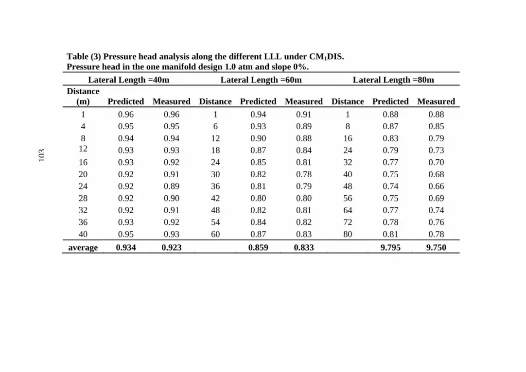
Table (3) Pressure head analysis along the different LLL under CM1DIS.

Pressure head in the one manifold design 1.0 atm and slope 0%.


Distance


1 0.96 0.96 1 0.94 0.91 1 0.88 0.88

4 0.95 0.95 6 0.93 0.89 8 0.87 0.85

8 0.94 0.94 12 0.90 0.88 16 0.83 0.79

12 0.93 0.93 18 0.87 0.84 24 0.79 0.73

16 0.93 0.92 24 0.85 0.81 32 0.77 0.70

20 0.92 0.91 30 0.82 0.78 40 0.75 0.68

24 0.92 0.89 36 0.81 0.79 48 0.74 0.66

28 0.92 0.90 42 0.80 0.80 56 0.75 0.69

32 0.92 0.91 48 0.82 0.81 64 0.77 0.74

36 0.93 0.92 54 0.84 0.82 72 0.78 0.76

40 0.95 0.93 60 0.87 0.83 80 0.81 0.78

average 0.934 0.923 0.859 0.833 9.795 9.750

103

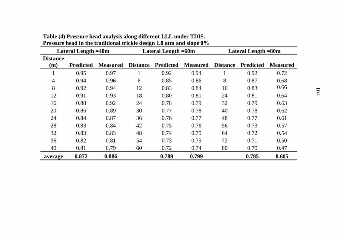
Table (4) Pressure head analysis along different LLL under TDIS.

Pressure head in the traditional trickle design 1.0 atm and slope 0%


Distance


1 0.95 0.97 1 0.92 0.94 1 0.92 0.72

4 0.94 0.96 6 0.85 0.86 8 0.87 0.68

8 0.92 0.94 12 0.83 0.84 16 0.83 0.66

12 0.91 0.93 18 0.80 0.81 24 0.81 0.64

16 0.88 0.92 24 0.78 0.79 32 0.79 0.63

20 0.86 0.89 30 0.77 0.78 40 0.78 0.62

24 0.84 0.87 36 0.76 0.77 48 0.77 0.61

28 0.83 0.84 42 0.75 0.76 56 0.73 0.57

32 0.83 0.83 48 0.74 0.75 64 0.72 0.54

36 0.82 0.81 54 0.73 0.75 72 0.71 0.50

40 0.81 0.79 60 0.72 0.74 80 0.70 0.47

average 0.872 0.886 0.789 0.799 0.785 0.605

104

عزا تعقعمتوووووووووو ع وووووووووو عال وووووووووو تعالخطوووووووووو طعال العوووووووووو ع ل وووووووووو عال وووووووووو ع وووووووووو ع وووووووووو عا وووووووووو بهووووووووووووووصاع وووووووووووووو ع ووووووووووووووص عالت وووووووووووووومعم تعع(TDIS)ا خوووووووووووووواتعموووووووووووووو عال وووووووووووووو عالت عوووووووووووووو تع

سووووووووووو ل تعل ووووووووووو عت عوووووووووووفعا خ ووووووووووو عال ووووووووووو طع ووووووووووو ع ه عووووووووووو تعخطووووووووووو طعال العووووووووووو تعبشووووووووووو فع ووووووووووو فع عووووووووووو فعل ووووووووووو عصلووووووووووو عاع ووووووووووو عا عا خت ووووووووووو تعبوووووووووووع عال وووووووووووع عا بووووووووووواع ا قووووووووفعل وووووووو عطوووووووو فعالخطوووووووو طعل وووووووو عموووووووو عال وووووووو طع الت ووووووووا ع ووووووووتعم ب لوووووووو عموووووووو ع

وووووووووو عب وووووووووو عال وووووووووو تع اع وووووووووو ع وووووووووو ع توووووووووو عم عوووووووووو عا وووووووووو ع عل معوووووووووو ععلوووووووووو االخ ووووووووووووو عالهع ا لعووووووووووووو ع اع ووووووووووووو عبم ا ووووووووووووو عقوووووووووووووع عال ووووووووووووو طعالم سووووووووووووو عم م عووووووووووووو ع

-Hydro)بوووووووووووو ل ع عالتوووووووووووو عتوووووووووووو ع سوووووووووووو به عب اسووووووووووووط عبا وووووووووووو م عالم وووووووووووو عالمسووووووووووووتخ Calc)إل وووووووووووواالعال سوووووووووووو ب تعالهع ا لعوووووووووووو عبهوووووووووووو عت قوووووووووووو عموووووووووووو عسووووووووووووعت عل وووووووووووو عاا عع

ل ووووووووع عالمت ق وووووووو عباسووووووووتخ ام عبوووووووو ل ع عال عوووووووو عالتوووووووو عتوووووووو عال اقوووووووو ع عوووووووو عا بووووووووتعت وووووووو ا عات سووووووووووووووو تعالخ ووووووووووووووو عقع سووووووووووووووه عخووووووووووووووو فعا وووووووووووووواالعالت ووووووووووووووو ا عالم م عووووووووووووووو ع قوووووووووووووو ع

الهع ا لعووووووووووووووو عا خووووووووووووووواتع م موووووووووووووووفعا ت معووووووووووووووو ع ال مووووووووووووووو عالخ ووووووووووووووواتع م ووووووووووووووو فعا عموووووووووو عال بووووووووو ع ا لعووووووووو ع وووووووووو لاتعالمعووووووووو ع ا سوووووووووم ع اع وووووووووو عاقت ووووووووو ع عبووووووووو ل

ووووووووو عتزعووووووووو عق وووووووووع علووووووووو عال ووووووووو عالت عووووووووو عا عإ ووووووووواالع وووووووووص عالت ووووووووومعم تععتط ووووووووو عت ا عا هوووووووووو عت وووووووووو عصلوووووووووو ع عوووووووووو عع وووووووووو ع وووووووووو عا ابوووووووووو عا وووووووووواعب سووووووووووتخ ا ع ووووووووووص ع

ممووووووووو عع وووووووووو ع وووووووووا ا عتطبعوووووووووو ععالت ووووووووومعم تعالم لوووووووووو ع مووووووووو ع وووووووووو ع ا ووووووووو عب ل توووووووووو وووووووووص عال ااسووووووووو عب سوووووووووتخ ا ع وووووووووصاعالت ووووووووو عفع عووووووووو عل ووووووووو عسوووووووووبعفعالت ابووووووووو عبم ووووووووواعا ع

عموووووووووو عالمعوووووووووو ع اا وووووووووو ع ع ووووووووووفع ااسوووووووووو عصلوووووووووو ع وووووووووو عالم وووووووووو ط عالتوووووووووو عبهوووووووووو ع وووووووووو اع ال االعالم اع عالمست ع ع

9

باع ا قفعبت معم تعا خ ع ق عا ت ع صل عقعم عا خت تعبع عال ع عا ع-3 ال ا اعالم عب لم ا عب ل عالت ع تعل اتعب لت عط ع

مفعا ت مع عا ت عت ا عال ط تعل عط فعالخط طعال الع ع ع عزع عم ع-4ع عع11ب سب ع، عال ا اعع5 %5 عب ستخ ا عال ت عالت عط عب عب لم ا % CM1DIS, CM2DISالم

ع ع عع-5 عالصتعع تم عل ععت س عا ت عت زع عالمع ت س عا ت مع عت زع عا سم (Fertigation)عالاتع ع تعت عم عخ ف

عع-6 ع ب عم ف عم عل لع عا ت ع عب سب ع9 8الصا عب سب ع8 %9، ع ال ط %عال ا اع53 3%،ع53 3 عالت عطععCM1DIS, CM2DIS %عب ستخ ا ب لم ا عب

الت ع ت عع-7 عب سب عالمع عاست م ف ع ل ع9 7زع عع3 6، عال ب ، علم ف %ع8 %1

ل ع عالت عطعال ت ععCM1DIS, CM2DISلم فعال ط عب ل ا اعالم ع،ع9 8ل سم عال تا ع ع،ع ب سب عع8 8،ع8 13زع ع ل عاست م فعا سم عب سب عع-9

ع CM1DIS,، CM2DISال س ت ع الب ت س عب ل ا اعالم %عل عم عالسم ع 8 9 ب لم ا عب عالت عطعالت ع ت

ال ععب س عت لع عا ت جعم فعالصا ع) ع (عا تعال ت عا عا اب ع تع-8 %عل ع عالت عطعالت ع ت ع13باستخ ا عال ا اعالم عب سب عتخطتع

ع) ع / ع-13 عالمستخ م عالات عمع ع عا قت تعم عال خف ع ع ع3قعم )عال ا اع ععCM2DISا اعب ستخ ا ،CM1DISعالت عطعال تعع عب عب لم ا الم

%عل عالتاتع ع53%،ع51ب سب ع(ع عا اع3م ع عال خفعالطبع عم ع عمع عالاتعالمستخ م ع) / قعع-11

تعب سب عب لم ا عب عالت عطعالعCM2DIS،ععCM1DISالم عب ستخ ا عال ا اع %ت تع عم 5 4%،ع8 3

ع م عع :ع ب لعل عت عال ت عع ت عالت ع عب ستخ ا عال ا اعا اعا ت مع ع ع فع ت وووووووو عبطووووووووو ب ستخ ا عخطع الع(CM2DIS)ل عال ا ا عالم عم عال عع ع ع

ط فعخطع ال ع ت ع ستخ ا عبع(CM1DIS) ع ل عال ا ا عالم عم عال عع عمتا،عع93عط ف عالسب عووووو ع ع ع (TDIS)متاع ع ل عال عالت ع تعع43،ع الط فعمتاعل خطعال ال ع63

عع فووووطل ع ع) ع عت ع س ب (عوووووو ق عا ت ووووووووووووو عب ستخ ا ع ص عال ا اعا خ ا ع عصل ع ععع

8

ع عالتاتع عالت مع ع ،ع38 8،ع17 8 ع ع تعال ع ع)ع CM1DIS لعب ع ع3 / ع38 8 عم عا قت ت عال خف عل عا قف عال عم ع ت عبع م )

ت مع ع عTDIS(عل عاستخ ا ع3 / ع83 1ع،89 1،ع13 8المع عالمستخ م ع)ل ععمتاع93،ع63،ع43ب ستخ ا عاط افعل خط طعال الع عع عالت عطعالت ع ت

عالتاتع ع اإلضافة العلمية الجديدة:

عتسم ع عت معم تع ع عا عطاع عال تعل عالت عط ع تط عا ال ا اعالم ع م عع :

.( (CM1DIS خطعم ع ل ع ا عمت فأ :ع ا ا عم عب ستخ ا ع ( CM2DIS) ع :عب ستخ ا عخطع عم ع ل ع)خطع عت زع عم ع (ع

(Control)(TDIS) ل :عت عاخصع عالا عب لت عطعال تعل م ا عااب :عإستخ ا عبا م عم علت عع ع ص عال ا اعالم ع ع ا لع ع ع م ا ته عب ع

.Hydro calc)ع ع عت ع س عال ع عالمت ق عب ستخ ا عالبا م عع تت الت عطعالProgram)م ا ته عب ل ع عال ع عالت عت عقع سه عم م ع ع

ععت عع عما ع) ف ع اا ع عالم س عالصا عم ف عل ع ع عت اب عإ اال خ مس : زاالت عت تعالاتعب لت عط(

:التوصياتعم عال عم عع :أ تعاستخ ا عت معم تعال ا اعال

عا خ عال طعالم عب ه ع عالخط طعال الع ع عالت عطعع-1 م ل عمش ع ت ع عاط افعخط طع الع ع ت عع63ال تع صل عباستخ ا ع ا ع ع، ع93متا

متا عمش عع-8 عم ل ععت عل ع تعتسته عالت عالات ع عتش عف عط ق ت عا

تع بعا ع اعب ل عالت ع تعل عم ل ع طع ت ع عات ا خ عال ل ه عبت عفعل عال اتع) عالمطاق عالم ع (عا عبا عسال عم ت اعالاتع

)ال عزف( ع

7

الذرة المحسن وراثيا تحت تعديالت تنتا محصول رابعا: التحليل االقتصادي ال ع:ععتنظام الري بالتتنقيط

عالت عتاتب ع عال ع عتس ل عالت ع تعالزاالع عالا عال ع ع المط ا طعب ل عخ ع ا ع بعا عل ست م اعم عخ فعإ ت جعالم عفعبطا عأ ع أ فععا شع لع عم ع عا ع ا سم ع الط ق عالمع ع مع ت ع عا قت عطاع ل المستخ م ع ع فعت ع ع ع عت ع عممعزاتع ع عل ع ب لت ل عت عزع ع

ع ا اب عالم تم عل عأس ع ا ع عم فعالا ا ست م ااتععالت مع ععععععععع عطاع عل عالات عا عتبع عاقت ع عالمستخ م عال بت عف

CM2DISع)ع عااب ع عا ل ع1743 ع1653، ع / ا عع1684،ع ع عالتاتع عالت مع عب ع ل ع ع ع عا اب عع CM1DIS/م س (

ع1733) ع1681، عل عع1638، عا قف عال عم ع ت عبع م ع/م س ( ع / ا ت مع ع عTDIS ع ع/ ا ع/م س (عل عاستخ ا عع738،ع774،ع943ا اب ع)

ل ععمتاع93،ع63،ع43ب ستخ ا عاط افعل خط طعال الع عع عالت عطعالت ع تعالتاتع ع

(ع ع3/ عال خفعا قت تعم ع عالمع عالمستخ م ) ع ععععععععععععع(ع لع3 ع / ع43 3،ع41 3،ع43 3)عCM2DISال عقعم عب ستخ ا عالت مع عع ع عالتاتع عالت مع ع)ع CM1DISب ع48 3 ع ع تعال ع ع4 3، ع38 3،

عالمع ع3 ع / ع عم عا قت ت عال خف عل عا قف عال عم ع ت عبع م )ت مع ع ع عTDISا ع(عل عاستخ 3 ع ع/ ع19 3،ع18 3،ع81 3المستخ م ع)

عالت ع ت ععالت عط عال الع عل خط ط عاط اف ع43ب ستخ ا ع63، ل ععمتاع93،عالتاتع ع

(عاخصع ع3 / ( عال خفعالم تعم ع عمع عالاتععات ع عم ع عالاب ع عال خفعا قت تعم ع عالمع ع ع ع تع

ع(3 / ع39 8،ع18 8،ع83 8)عCM2DISال عال ع عب ستخ ا عالت مع ع

6

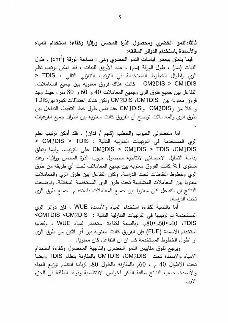
ثالثا:التنمو الخضري ومحصول الذرة المحسن وراثيا وكفاءة استخدام المياه ععواألسمدة باستخدام الدوائر المغلقه:

(ع،عط فعcm2 عم ععت عبب عقع س تعال م عالخ ا ع ع:عمس عال اق ع)ععع ع ع،عل عا اا عل ب تع، ام عتاتع ع عال ب تع)س (ع،عط فعال اق ع)س (

ع ع: عالت ل عالت زل عالتاتع ع عالمستخ م عالخط ط ع اط اف >ععTDISالا CM1DISعع <CM2DISعالم م ت عع ع مع عبع عم ع ع ا ع ع ت

متاا،ع ع ع عع93 عع63 عع43الت لفعبع ع مع عطا عالا ع مع عالم م تععTDIS تع بعا عبع ل ع عاخت عCM2DIS،ع CM1DIS ا عم ع عبع ع

ل ع عط فعخطعالت عط عالت اخفعبع ععCM1DIS عCM2DIS ع عم ع طا عالا ع الم م تعت عأ عال ا ع تعم ع عبع عأط افع مع عال الع تع

عتاتع ع ع عأم ع ع، ع ا ( ع/ عال ب ع ال ط ع) عم ل ام

عالت لع عالت زلع عالتاتعب ت ع عالمستخ م عالا ع: TDISعع <CM2DISعع<CM1DISع ،TDISع<CM1DIS عع <CM2DISععت عع ع عم عالتاتع ل

ع ل ع ع اا ع ، عالم س عالصا ع ب عم ف ع ت ع عا عالت عف ب اس %ع تعال ا عم ع عبع ع مع عالم م تعت تعأ عطاع عم عطا ع1مست تع

فعبع عطا عالا ع الم م تعالا ع خط طعال ط تعت تعال ااس ع عالت لم ع عبع عالم م تعالمتش به عت تعطا عالا عالمستخ م عالمخت ع ا تعال ت عا عالت لفع عم ع عبع ع مع عالم م تعب ستخ ا عع مع عطا عالا ع

ت تعال ااس عع ع ا سم عالمع عاستخ ا عل ل عب ل سب عالا ععWUEأم ع ا ا ع ا ،<عCM1DIS<عCM2DISم عت عتاتعبه ع عالتاتعب تعالت زلع عالت لع ع:ععالمستخ TDISع ع93 <63 <43، عالمع عاستخ ا عل ل ع ب ل سب WUEع ل عع ،

ا عال ا ع تعم ع عبع عأ عا ع عم عطا عالاتعع(FUE)استخ ا عا سم ععا عاط افعالخط طعالمستخ م ع م عا عا عالت لفع عم ع ع

عاستخ ا ع ع عالم فع ل ا عت عم عع عال م عالخ اتع ا ت ع عت تع ع ا سم ع CM2DISا مع ،CM1DISعع عب اع ععTDISب لم ا

ع عا ط اف عع43ت ت ع، ع63 عب لط ف عب لم ا عالمع ع93 عت زع عا ت علزع عال ط ق ع عال زلع ا سم ع س عال ت عس ل عالص اعلخ ا عا ت مع ع اق

عا ف عع

5

عالت لفعبع ع-4 عDICت عا ،LLLعمست تعع عل عال تع1 عم ع عال ع %ل ععCM2DIS X LLL1،ع TDIS X LLL3 ال ع ع تعل عالت ل تعالت لع :

التاتع علت ا عال ط تع-5 عام عتاتع عع(qd)ب ل سب DIC ع ،LLLعالتاتعب تعع

عLLL1>LLL2>LLL3،ع CM2DIS >CM1DIS> TDISالت ل ع عالت لع :عع عت ا عالخط طعال الع عام عتاتع عع(QL)ام DIC ع ،LLLعالتاتعب تعع

ع عالت لع : ع CM2DIS>CM1DIS>TDISالت ل ع ،LLL3>LLL2>LLL1ع % 1 عا عال ا ع تعم ع عل عمست تع

ل عمست تعع ع عم ع qd، QLل ع عم ععLLL،عDICت عاعالت لفعبع ع-6لتا/س ل (ع،عع16 8،عع19 4 تع)عQL ،عqd% عال ع عال تع ال ع عل عم ع1ع883) عع486، عالت ل ت عل عالتاتع عل ،عCM2DIS X LLL1لتا/س ل (

TDIS X LLL3 ع ا تع ت عا عال ا ع تعم ب ل عع(qvar) ق عت ع س عاخت عالت ا ععاستخ ا عاستخ ا عالط فعبع عال ع عا باع ا قفع ع ع93مع عال تعم عل ا

)الت ع ت( عTDISت تعاخت تعم مفعا ت مع عم ع ع ع ععال ا ا عالم عا عط فعالخطعال ال عع-7

عاستخ ا ع. ل عالت اخ تعاع ل عالس الع تعال ا عم ع ع عم عبع ه ع عال ع عم عم عم ع(CM2DIS) ا ا عقع ع ت عا ت مع ،عع73 85مف

ع45 98 ع عال ععع85 93، عاستخ ا ع ل ،%(CM1DIS)عع ،عع74 87 تع،عع87 99 تعع(TDIS)%،عبع م عب ستخ ا عال ععال تععع33 88،ع عع14 85متاعل عع93،ع63،ع43%عت تعأط افعالخط طعال الع عع53 93،ع عع73 94

ع عم ع عمست ت عل عل اع1التاتع عبع عال ا عم ع ع% ع ت عال ااس مف ب ل سب علم مفعا ت مع عع

ثاتنيا: مقارتنة القيم المتوقعة للضغط )بواسطة برتنامج محاكاه( بالقيم التى تم عقياسها:عع عإستخ ا عDICل ،LLLعبا م عع عب اسط عالمت ق عال ع علم ا ع عع(Hydro-Calc) الم عم م ع ، عقع سه عت عالت عال ع ع ع اع عا

%عبع ع مع عال ع ع أ عا اا تع تعبسعط عبع ع1 ا عم ع عل عمست تعع LLL3XTDISم ع تعال ع عالمت ق ع الت عت عقع سه عباست لعالت لفع

4

عا ت مع ع عم مف ع س عت ع اع عالمخت ، عال الع عب لخط ط عالت س ع93،ع63،ع43 طعال الع عالمخت ع م مفعا خت عل ت ا تعل عط فعالخط

عمتاعب م عالت عطعب ل ا اعالم عالت ع تعل عالس ال ع وكاتنت اهم التنتائج كما يلي :

0.1أوال: القياسات الهيدرولية للدوائر المغلقة تحت الدراسة بضاغط تشغيل % :1ض. ومستوى اتنحدار

ع -1 عالت عط عخط عط ف عل عالط ق ع اق ع ااس ع ق ععت ع عالم ال طا ت ع سال عالساع ع،ع طعالسال ع اش اتعال ت عال عا عالخ ع ه ع عم عل اع ق عا ت ع تعت خصع عا ت ع ع عام عتاتع ع عم ع

ع عالمستخ م عالات ععDIC ا ا ع اط اف عالت عط عخط ط عال الع ( )الخط طLLLعع :ع ع م ععCM2DIS>CM1DIS>TDISت زلع ،40m>60m>80mع-ع

ع عم ع عمست ت عل عم ع عال ا ع ت عال ا اعع1 ا ع عا اع عبع % . خط طعالت عط

ل عال طعالم ع سال عالساع ع LLL ،عDICع ت عاعالت لفعبع ع عم-8عال تع عال ع عالم ع عمست ت ع عل عم ع ع عاع عالسال ط

ع386 3 / ع عع37 1 ،عع5 8 سال عالساع ع طعالسال ع)ل طعالم ععالت ل تع) عل ) CM2DIS X LLLع ،TDIS X LLL3 عع TDIS X

LLL3(ع ع ت عال ع عال ع عبع م عع35 6( عع583 3 ، ع عل عع19 3 / ) عع TDIS X LLL3ت اخ تع) ،TDIS X 1LLL عع TDIS X LLL3عل ع )عالتاتع

بع عال ع عا باع ا قفعل عط فعع(Hvar) طعالم ع ق عت ع س عاخت عالالخط طع عال تعالمخت ع اش اتع ت عال عا عا خت تع تعم ب ل ع ع

ع TDIS،عCM1DIS عت تع عم ع93 مع عال تعم عل اعاستخ ا عالط فع ق عا ت عام عتاتعب عل عصل ع ع عاخصعات عل س عل عالخ عع-3ا خاتعل عل ق عل سع عبع عال طع ق عا ت ع عام ععلهع ا لع ا

ع DICتاتع ، LLLعالت لع :عع عالت ل ع عالتاتعب ت TDIS>CM1DIS>CM2DISع ،LLL3>LLL2>LLL1عبع عع عال ا ت

DICع، LLLع% 1م ع عل عمست تع

عع

3

ع عالت عطعالت ع ت ع ت جعم فعالصا عت تع ص عالت معم تع م ا ته عب .موقع التجارب

أ اعتعالت ا عالم م ع عل عأ هز عالا ع م اتعم مفعاختب ااتعالاتعع.،عم اع عز ال ،عم ه عب عاله س عالزاالع ،عما زعالب عالزاالع ،عال

ع ععال ع أ اعتعالت اب ع م ع، عالزاال ع ع عم ع ع ع عمزال الع ،عإل عا ماع ع اب عف، عالمت عال ع ت ع ع ، ع لا عط ف ع73 37خط ط

ع عمست تعسط عالب ا عع118mع (387feet) ب عاات عع16 98ع،شم ععالتجارب المعملية:

عم ا ته ع ع ت عم م ع عال ا اعالم عاختب اع لع عم عت معم تع ص ت ل عالت عطعالت ع تع ع لت ل :

(CM1DISقه باستخدام خط ماتنيفولد واحد متصل )األول :دائرة مغلام ا عم عالمع عم ع ط عع(Manifold) ع ص عال ل عع خصعخطعالت زع ع

ا عب لخطعت تعالا عس ،ع م عا عخطعت زع عع عخطع ا عتت فعب عخط طعال الع تعبش فعتب ل عب ع عع عل عالخطعال ال ع طتع عات فعا ا م ع

عل خطعال ال ع ا خاتع ط عخا جعال عالم ع ل عما عاخات ط ع خ فع (. CM2DISالثاتني: باستخدام خطين ماتنيفولد )خطين توزيع متنفصلين( )

ع ع عم ع ل ( ع)خطع عم ع عت زع عخطع عال ل ع ص ع عستخ م هم ععت فعب لخطعت تعالا عس ع ل فعخطعم هم ع ه ع عخطع عت فع فعخطعم ع

ل الع عب عل ع طتع ع ع عا ع عال طتع عل فعخطع ال ع ع ط عالخط طعاع خ فعل خطعال ال عع

(Control)( للمقارتنه TDISالثالث: تم اخذ تنظام الري بالتتنقيط العادى )ع ع ق عال الع ت علخط ط عأط اف ع عال تعع(Laterals)استخ مت ع مع

ع ع عع43الس ب ع عع63، ع عع93، عت تع ف ع تمتعمتاا عالم عال ا ا ععم عالم ا عب عالت عطعال ت عع

ق عت عقع عال طعالم عل عط فعالخط طعال الع عب اسط عل ا ع(،ع(Manifolds طعابا ع بمس ل عل ا اتع طعم بت عل عخط طعالت زع ع

ع ت ع س عقعم عال عب ت عبم ل ع ز ع لع ،ع ت عقع عم تعالت عم م ع عباست ب فعالت ع عا ا ع ععت عال ز ع ت ع عال ع ،ع م عام

ع

2

ع الملخص العربي

عم فع عالا عب لت عطعأ عم ع تعإلع عت ل ع عالا ع ل عال ع عم عالممعزاتع م عع ب عب عالمش فع الم ق تع مش عا خ عال طع

ع عالت عت عاقتاا عتط عاعال ا اعالم ع صل عالم ع ع ه ع عخط طعالا عال الع ص ع عل عل ت عب لت عط عل ا عالت ع عال عإل عالت ع ت عب با عالم اع ع عال اال ع عالت عط عب عتا ت عالت عالمس ت ع تتزاع المش ع ب ع عال ه عأش ا عا ع عالطاع ع ص عت ع ع ع، ع ا ع بعا بم ت

عا عع ت عالا عب لت عطعل ع عا ع ع ع ا عال ع ع الم عف الخ اع عبتاطع ع زلعم عالتاب ع طع تب عا زالعا خاتع عط فعالم س ع ع ت ع

عل ع صاعالتاطع عال ز ع ا عل ع ع مش فعق ع الهدف من الدراسة:

عل ع ه ع ع فعلمش عا خ عال طعالم عه عالب عال عاع عععع معم تعتسم ع ا اعم عالخط طعال الع عل عالاتعب لت عطع صل عب قتاا ععت

عأ ع)ع- : عخطع عت زع عالخط طعال الع عManifoldاستخ ا علت صع عم ع )(ع ا عمت فعلت صع عالخط طعManifoldاستخ ا عخطعت زع ع)ع-م عال بع ،ع

ال عالت ع تعل م ا ،ع استخ ا عم م تعاستخ ا عع-جع–ال الع عم عال بع عع عمخت ع الع عخط ط ع43ب ط اف ع63، عا ت مع عع ،ع93، عال عال ف به

ا عالم عبع عل عت معم تعل ا اعم ع عم ا ته عب عالت عطعال تعع عت ع عالم عف، عل عا ع عال ا عال ع عال ا ا ع ص عتطبع عاستخ ا

عاس عت عاع ص عالت معم تع الم م تعل عالخ عالت لع : اععا ت ،ع -1 ع ق ع، عال ط ع عالهع ا لع عالخ عب م م ع

عا خت ع عم مف عال ط، عت ا عالسال ، ع ط عالساع ، سال لت ا عال ط،عت ا عالخطعال ال ،عم مفعا ت مع

عال ت -8 ع م ا عبا م عم عالت ا ععاستخ ا عب ع الم س ب الم س الم م ع عب ل ع عالمت ق عب اسط عبا م عالم ع الصتععسم

(Hydro-Calc)ع ع عب عالخ عالخ اع ،ع ا ت ع عم فعالصا ع ال ط ،ع

ع ع ووت لع عا قووووووفعل ت ووووووووووووووفعت عوو ،ع لمووووو فعالمع ع ا سموووووو ل عاست موووووو

جامعة عين شمس

ةـــة الزراعـــكلي

رسالة دكتوراه

منصور ىعبد الغن ىعبد الغنب : هاني ــالـــاسم الط

اعتبارات تصميمية للدوائر المغلقة لنظام الري بالتنقيطعنوان الرسالة:

)ميكنة زراعية( ة : دكتور فلسفة في العلوم الزراعيةــــاسم الدرج

لجنة األشراف:

عبد الغني محمد الجندي د.

قسم الهندسة الزراعية، كلية الزراعة، جامعة عين شمس، المتفرغ أستاذ الهندسة الزراعية

)المشرف الرئيسي(

يوسف طايلد. محمد ، المركز الحقلي والري، قسم العالقات المائية متفرغالالعالقات المائية فيزياء التربة وأستاذ

للبحوث وميالق

ديفيد انتوني ليتفوتد. جنوب الينوى بكاربونديل، الزراعية، كلية الزراعة، جامعة والتربة والنظم أستاذ النبات

.ةالينوى، الواليات المتحدة االمريكي

2116/ 9/ 00 :تسجيلتاريخ ال

الدراسات العليا

أجيزت الرسالة بتاريخ ختم اإلجازة

26 /2 /2012

موافقة مجلس الجامعة موافقة مجلس الكلية

/ /2012 /2012/

اعتبارات تصميمية للدوائر المغلقة لنظام الري بالتنقيط

عع

رسالة مقدمه من

منصور ىعبد الغن ىلغنعبد اهاني

2111 المنوفية،جامعة ،راعية (زعلوم زراعية ) هندسة بكالوريوس

2116 ،جامعة عين شمس ،ماجستير علوم زراعية ) ميكنة زراعية (

ع للحصول علي درجة

في العلوم الزراعية ةدكتور فلسف

) ميكنة زراعية (

قسم الهندسة الزراعية

كلية الزراعة

شمسجامعة عين

1022

Documents

Design considerations for closed circuits of drip irrigation system. PhD: Thesis, Faculty of Agriculture, Agric., Ain Shams university, Egypt