Embed Size (px)
Citation preview

Design of a Wireless Power Transfer System using
Electrically Coupled Loop Antennas
Shyam Chandrasekhar Nambiar
Thesis submitted to the Faculty of the
Virginia Polytechnic Institute and State University
in partial fulfillment of the requirements for the degree of
Master of Science
in
Electrical Engineering
Approved:
William A. Davis
Dennis G. Sweeney
Disapproved:
Majid Manteghi, Chair
February 19, 2015
Blacksburg, Virginia
Keywords: Wireless power transfer, Implanted antennas, Electrically Coupled Loop Antenna,
Negative resistance oscillators
Copyright 2015, Shyam Chandrasekhar Nambiar
Design of a Wireless Power Transfer System using Electrically Coupled Loop Antennas
by Shyam Chandrasekhar Nambiar
Abstract
Wireless Power Transfer (WPT) has become quite popular over the recent years. This thesis
presents some design challenges while developing a WPT system and describes a system-level
methodology for designing an end-to-end system. A critical analysis of contemporary research
is performed in the form of a literature survey of both academic and commercial research to
understand their benefits and demerits. Some theoretical notes are presented on coupled-mode
theory and coupled filter theory and the problems concerning WPT analyzed using these mod-
els. The need for higher power transfer efficiency (PTE) and power delivered to load (PDL) is
studied using these models. The case for using magnetic antennas over electric antennas when
surrounded by lossy media (specifically for the case of human body tissues at various frequen-
cies) is made using some theoretical models and simulation results. An Electrically Coupled
Loop Antenna (ECLA) is introduced, studied and designed for two main WPT applications,
viz. free space transmission and that of powering implanted devices. An equivalent circuit
is proposed to better understand the coupling effects of the antennas on a circuit level and to
study the effect of various environmental and structural factors on the coupling coefficient.
Some prototypes were created and measured for the two use cases of free space and implanted
applications. In order to complete the system design, a negative resistance-based oscillator is
designed and fabricated, that incorporates the antennas as a load and oscillates at the required
frequency. Some changes in load conditions and power handling are studied by the use of
two circuits for free-space (high-power) and implanted (low-power) applications. Finally, the
salient points of the thesis are re-iterated and some future work outlined in the concluding
chapter.

“Education is a progressive discovery of our own ignorance.”
Will Durant
iii

To my family
iv

Acknowledgements
Firstly, I would like to thank my advisor, Dr. Majid Manteghi, for giving me the opportunity
to work on this project and for his guidance and practical advice throughout this project. I
would also like to thank my committee members, Dr. William Davis and Dr. Dennis Sweeney,
for taking the time to mentor and guide me through this journey and enriching my experience
while doing so. I would like to thank all of them for their generous patience while evaluating
my thesis and helping me along in generating this document.
The journey through my Master’s degree was made all the more rigorous, challenging, edu-
cational and enjoyable through the many courses that I took up and the wonderful professors
who taught them. I must also thank the Bradley Department of Electrical and Computer En-
gineering at Virginia Tech for sponsoring me as a Teaching Assistant and letting me influence
many young lives through teaching ECE 3105, 3106 while learning even more from bright, in-
quisitive minds. I am grateful for the wonderful environment and people of Virginia Tech who
have nourished me on my path as a better engineer and moreover, a better person.
I owe my gratitude to the Virginia Tech Antenna Group members with whom I have been lucky
to have worked for the past two years. I would especially like to thank Reza for his brotherly
mentorship, Mohsen for his insightful comments and Ali for his help with simulations. I am
also thankful to Roy for our friendly discussions and his help with the writing of my thesis.
Lastly, but certainly not the least, I would like to thank my parents for their faith in me (I finally
made it!); my sister and brother-in-law for their generous advice and gracious help; my fiancee
for being patient and loving (thank you, Sonu, for being there when I needed you most); and
my close friends for their never-ending love and support. The past two years have been tough
for me but tougher for them still and I owe them my deepest thanks.
v

Contents
Abstract i
Acknowledgements v
Contents vi
List of Figures viii
List of Tables x
Abbreviations xi
1 Introduction 11.1 History . . . . . . . . . . . . . . . . . . . . . . . . . . . . . . . . . . . . . . . . . . . 11.2 Motivation . . . . . . . . . . . . . . . . . . . . . . . . . . . . . . . . . . . . . . . . . 31.3 Objectives . . . . . . . . . . . . . . . . . . . . . . . . . . . . . . . . . . . . . . . . . 31.4 Thesis Organization . . . . . . . . . . . . . . . . . . . . . . . . . . . . . . . . . . . . 4
2 Literature Review and Theoretical Background 62.1 Research Trends and Theoretical Perspectives on Design . . . . . . . . . . . . . . 6
2.1.1 Review of Trends and Types of WPT . . . . . . . . . . . . . . . . . . . . . . 62.1.2 Coupled-Mode Theory . . . . . . . . . . . . . . . . . . . . . . . . . . . . . . 92.1.3 Filter Theory . . . . . . . . . . . . . . . . . . . . . . . . . . . . . . . . . . . 122.1.4 Comparison . . . . . . . . . . . . . . . . . . . . . . . . . . . . . . . . . . . . 14
2.2 Overview of Industrial Standards . . . . . . . . . . . . . . . . . . . . . . . . . . . . 152.3 Implanted Antennas: Electric vs. Magnetic Antennas in Lossy Media . . . . . . . 17
2.3.1 Overview and Motivation . . . . . . . . . . . . . . . . . . . . . . . . . . . . 182.3.2 Theoretical Results . . . . . . . . . . . . . . . . . . . . . . . . . . . . . . . . 212.3.3 Simulation in FEKO . . . . . . . . . . . . . . . . . . . . . . . . . . . . . . . 31
2.3.3.1 Simulation Results . . . . . . . . . . . . . . . . . . . . . . . . . . . 33
vi

Contents vii
2.3.4 Study Conclusions . . . . . . . . . . . . . . . . . . . . . . . . . . . . . . . . 34
3 Antenna Design 393.1 Introduction . . . . . . . . . . . . . . . . . . . . . . . . . . . . . . . . . . . . . . . . 393.2 Electrically Coupled Loop Antenna . . . . . . . . . . . . . . . . . . . . . . . . . . . 40
3.2.1 Antenna Characteristics . . . . . . . . . . . . . . . . . . . . . . . . . . . . . 423.3 Development of an Equivalent Circuit . . . . . . . . . . . . . . . . . . . . . . . . . 443.4 ECLA Variants and Design Iterations . . . . . . . . . . . . . . . . . . . . . . . . . . 47
3.4.1 ECLA in Free Space . . . . . . . . . . . . . . . . . . . . . . . . . . . . . . . 483.4.2 ECLA in Implanted Applications . . . . . . . . . . . . . . . . . . . . . . . . 52
4 System Design 654.1 Overview . . . . . . . . . . . . . . . . . . . . . . . . . . . . . . . . . . . . . . . . . . 654.2 Oscillator Design . . . . . . . . . . . . . . . . . . . . . . . . . . . . . . . . . . . . . 66
4.2.1 Negative Resistance Oscillators . . . . . . . . . . . . . . . . . . . . . . . . . 674.2.2 Mathematical Description . . . . . . . . . . . . . . . . . . . . . . . . . . . . 67
4.3 Simulation Results . . . . . . . . . . . . . . . . . . . . . . . . . . . . . . . . . . . . 714.3.1 Implanted Applications . . . . . . . . . . . . . . . . . . . . . . . . . . . . . 734.3.2 Higher Power/Efficiency Design . . . . . . . . . . . . . . . . . . . . . . . . 774.3.3 Free-space Application . . . . . . . . . . . . . . . . . . . . . . . . . . . . . . 804.3.4 Tuning the Oscillator . . . . . . . . . . . . . . . . . . . . . . . . . . . . . . . 84
4.4 Fabrication . . . . . . . . . . . . . . . . . . . . . . . . . . . . . . . . . . . . . . . . . 85
5 Conclusions and Future Work 895.1 Conclusions . . . . . . . . . . . . . . . . . . . . . . . . . . . . . . . . . . . . . . . . 895.2 Future Work . . . . . . . . . . . . . . . . . . . . . . . . . . . . . . . . . . . . . . . . 90
Bibliography 93
A ADS Techniques 101A.1 Introduction . . . . . . . . . . . . . . . . . . . . . . . . . . . . . . . . . . . . . . . . 101A.2 Test Bench Creation for Equivalent Circuit Optimization . . . . . . . . . . . . . . 101A.3 ADS Non-Linear and General Techniques References . . . . . . . . . . . . . . . . 103
B MATLAB Codes 104B.1 Introduction . . . . . . . . . . . . . . . . . . . . . . . . . . . . . . . . . . . . . . . . 104B.2 FEKO Field Extraction and Plotting . . . . . . . . . . . . . . . . . . . . . . . . . . . 104
B.2.1 NormalizedPowerPlotter.m . . . . . . . . . . . . . . . . . . . . . . . . . . . 104B.2.2 Functions . . . . . . . . . . . . . . . . . . . . . . . . . . . . . . . . . . . . . 107
B.3 Stability Analysis, Negative Resistance Termination Network for Oscillator Design108B.3.1 NegRes.m . . . . . . . . . . . . . . . . . . . . . . . . . . . . . . . . . . . . . 108B.3.2 Functions . . . . . . . . . . . . . . . . . . . . . . . . . . . . . . . . . . . . . 109

List of Figures
2.1 Overall system performance metrics . . . . . . . . . . . . . . . . . . . . . . . . . . 92.2 Coupled LC tank circuit system (Wei, X., Wang, Z., and Dai, H. (2014). A critical
review of wireless power transfer via strongly coupled magnetic resonances.Energies, 7(7):4316-4341. Used under fair use, 2015.) . . . . . . . . . . . . . . . . . 9
2.3 Equivalent circuit for magnetically coupled resonators (Hong, J.-S. G. and Lan-caster, M. J. (2004). Microstrip filters for RF/microwave applications, volume167. John Wiley & Sons. Used under fair use, 2015.) . . . . . . . . . . . . . . . . . 13
2.4 Comparison of useful parameters used in contemporary industrial designs . . . 162.5 Antenna Losses . . . . . . . . . . . . . . . . . . . . . . . . . . . . . . . . . . . . . . 202.6 Normalized power loss for muscle tissue inside radian sphere of (a) radius, b =
14.5 mm at 403 MHz (b) radius, b = 2.7 mm at 2.4 GHz and (c) radius, b = 1.9mm at 3.5 GHz . . . . . . . . . . . . . . . . . . . . . . . . . . . . . . . . . . . . . . . 24
2.7 Normalized radiated power ratio, P (N)(r, a), inside muscle tissue at 403 MHzfor (a) magnetic dipole and (b) electric dipole (c) Ratio of values shown in (a) to (b) 29
2.8 Normalized radiated power for various tissues vs. sphere radius, a, for fixedradiation distance, r (= 10 cm), at (a) 403 MHz (b) 2.4 GHz and (c) 3.5 GHz . . . . 30
2.9 Simulation setup in FEKO showing dipole and loop antennas inside muscle tissues 312.10 Flowchart describing steps to obtain MATLAB output from FEKO . . . . . . . . . 332.11 Simulated results for normalized radiated power ratio, P (N)(r, a), inside muscle
tissue at 403 MHz for (a) loop antenna and (b) electric dipole. (c) Ratio of valuesshown in (a) to (b) . . . . . . . . . . . . . . . . . . . . . . . . . . . . . . . . . . . . . 35
2.12 Comparison between theoretical and simulated results for normalized radiatedpower ratio, P (N)(r, a), inside muscle tissue at 403 MHz at r = 10 cm . . . . . . . 36
2.13 Total Poynting vector magnitude (in dB W/m2) and Current Distribution on theelectrically small loop antenna . . . . . . . . . . . . . . . . . . . . . . . . . . . . . 36
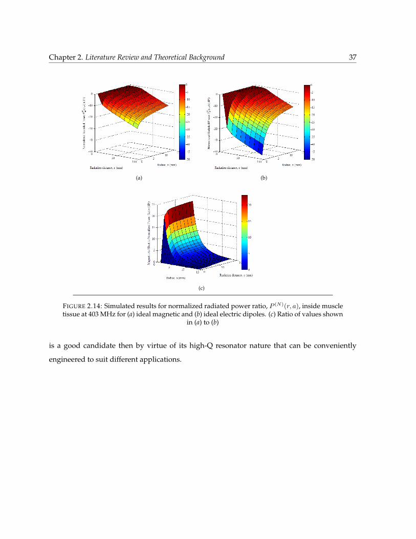
2.14 Simulated results for normalized radiated power ratio, P (N)(r, a), inside muscletissue at 403 MHz for (a) ideal magnetic and (b) ideal electric dipoles. (c) Ratioof values shown in (a) to (b) . . . . . . . . . . . . . . . . . . . . . . . . . . . . . . . 37
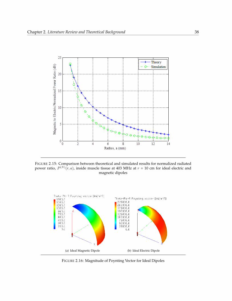
2.15 Comparison between theoretical and simulated results for normalized radiatedpower ratio, P (N)(r, a), inside muscle tissue at 403 MHz at r = 10 cm for idealelectric and magnetic dipoles . . . . . . . . . . . . . . . . . . . . . . . . . . . . . . 38
2.16 Magnitude of Poynting Vector for Ideal Dipoles . . . . . . . . . . . . . . . . . . . 38
viii

List of Figures ix
3.1 ECLA structure and design parameters . . . . . . . . . . . . . . . . . . . . . . . . 413.2 ECLA Gain in dBi . . . . . . . . . . . . . . . . . . . . . . . . . . . . . . . . . . . . . 433.3 |Etot|, |Htot| variation with r at θ = π/2, φ = 0 . . . . . . . . . . . . . . . . . . . . 443.4 ECLA equivalent circuit model iterations . . . . . . . . . . . . . . . . . . . . . . . 453.5 Gain and phase matched with an ECLA equivalent circuit model . . . . . . . . . 463.6 ECLA structural iterations and Current Density . . . . . . . . . . . . . . . . . . . 483.7 ECLA protoype and measurement results . . . . . . . . . . . . . . . . . . . . . . . 493.8 Ring ECLA simulation in FEKO for near-field . . . . . . . . . . . . . . . . . . . . . 503.9 Ring ECLA experimental setup . . . . . . . . . . . . . . . . . . . . . . . . . . . . . 513.10 Initial HFSS and ADS setup for implanted applications . . . . . . . . . . . . . . . 533.11 HFSS Results . . . . . . . . . . . . . . . . . . . . . . . . . . . . . . . . . . . . . . . . 543.12 Miniaturized ECLA prototypes using additional lumped capacitor where neces-
sary . . . . . . . . . . . . . . . . . . . . . . . . . . . . . . . . . . . . . . . . . . . . . 583.13 Miniaturized ECLA prototypes experimental setup in free space . . . . . . . . . . 593.14 Miniaturized ECLAs modeled in XF7 with a human body model at MICS band . 603.15 Miniaturized ECLAs modeled in HFSS for a pork-based phantom . . . . . . . . . 613.16 Experimental setup for a pork-based phantom . . . . . . . . . . . . . . . . . . . . 633.17 Medical applications . . . . . . . . . . . . . . . . . . . . . . . . . . . . . . . . . . . 64
4.1 General Oscillator block analysis . . . . . . . . . . . . . . . . . . . . . . . . . . . . 684.2 Two-port oscillator analysis . . . . . . . . . . . . . . . . . . . . . . . . . . . . . . . 684.3 ADS Circuit test setup for MRF559 for PBJT, AP and S-parameter ADS models
(VCE = 10 V and IC = 100 mA . . . . . . . . . . . . . . . . . . . . . . . . . . . . . 734.4 S-parameter curves for MRF559 for PBJT, AP and S-parameter ADS models
(VCE = 10 V and IC = 100 mA . . . . . . . . . . . . . . . . . . . . . . . . . . . . . 744.5 Two-port analysis ADS setup for 440 MHz . . . . . . . . . . . . . . . . . . . . . . 764.6 Two-port stability analysis for 440 MHz . . . . . . . . . . . . . . . . . . . . . . . . 774.7 Two-port analysis S-parameter data for 440 MHz . . . . . . . . . . . . . . . . . . . 784.8 Transient analysis ADS setup for 440 MHz . . . . . . . . . . . . . . . . . . . . . . 794.9 Time progression data for 440 MHz . . . . . . . . . . . . . . . . . . . . . . . . . . . 804.10 Frequency analysis of transient data for 440 MHz . . . . . . . . . . . . . . . . . . 814.11 Transient analysis ADS setup for High Power circuit . . . . . . . . . . . . . . . . . 824.12 Time progression and current data . . . . . . . . . . . . . . . . . . . . . . . . . . . 834.13 Frequency analysis of transient data . . . . . . . . . . . . . . . . . . . . . . . . . . 844.14 Two-port S-parameter analysis ADS setup for 39 MHz . . . . . . . . . . . . . . . . 854.15 S11, S22 . . . . . . . . . . . . . . . . . . . . . . . . . . . . . . . . . . . . . . . . . . . 864.16 Gain, phase data of S21 . . . . . . . . . . . . . . . . . . . . . . . . . . . . . . . . . . 874.17 Prototyped circuit for 39 MHz . . . . . . . . . . . . . . . . . . . . . . . . . . . . . . 88
5.1 Radiation Pattern for Coupled ECLA system at the two highest S(21) frequencies 91
A.1 Test Bench and Test Lab setup for creation of equivalent circuit in ADS . . . . . . 102

List of Tables
2.1 Values of Dielectric Constant and Effective Conductivity For Various HumanTissues at Different Frequencies . . . . . . . . . . . . . . . . . . . . . . . . . . . . . 25
3.1 Control of Frequency Response using ECLA’s Design Parameters . . . . . . . . . 423.2 Coupling efficiency vs. receiver antenna size . . . . . . . . . . . . . . . . . . . . . 52
x

Abbreviations
AUT Antenna Under Test
CMT Coupled-Mode Theory
ECLA Electrically Coupled Loop Antenna
BW BandWidth
FT Filter Theory
LTI Linear Time Invariant
MICS Medical Implant Communication Service
MoM Method of Moments
PDL Power Delivered to Load
PEC Perfect Electric Conductor
PIFA Planar Inverted F-Antenna
PTE Power Transfer Efficiency
RF Radio Frequency
SAR Specific Absorption Rate
WPT Wreless Power Transfer
xi

Nomenclature
∆ S-parameter discriminant
ε permittivity
η intrinsic impedance
ηopt CMT: optimum transfer efficiency
Γ CMT: damping factor; S-parameter analysis: reflection coefficient
κ CMT: coupling coefficient
µ permeability
σ conductivity
a CMT: complex amplitude
K Rollett stability factor
k FT: coupling coefficient
Q Quality factor
xii

Chapter 1
Introduction
1.1 History
Over the past decade, commercial products have become smaller and smaller while becoming
computationally more powerful. They have changed the way humans interact with the world
and the objects around them. This is the age of pervasive computing, and the effect of tech-
nology on our lives can be seen and felt by looking around us and noticing that we are almost
entirely dependent on our gadgets and machines. As human beings, we love technology and
creating tools and implements that make our life easier. Every year there are thousands of new
inventions that shape and make our lives more comfortable than it was the previous year. As
the number and complexity of these devices grows, we are faced with the problem of having to
power these devices and sustain their operation ever more efficiently. Even though battery and
power supply technologies (switched power electronics, High Voltage DC, etc.) have become
more efficient over the years, it is definitely more desirable to have a powering/recharging
solution as ubiquitous and convenient as wireless internet.
It is in this context then that the field of Wireless Power Transfer (WPT) has gained momentum
lately. However, efforts to transfer power wirelessly began with Heinrich Hertz’s experiments
1

Chapter 1. Introduction 2
with radio waves. Hertz used synchronously tuned resonant circuits to be able transmit us-
ing spark gaps possible (which are inherently wideband and were, therefore, outlawed in later
years by regulatory bodies). However, Tesla’s demonstrations at his residence and at exhibi-
tions were what truly captured the imagination of the public. Tesla’s method was to use his res-
onant transformers (or Tesla coils) [Tesla, 1900, 1914] for creating a zone of wireless power near
the transmitter. Tesla’s end objective was to provide free power to everyone over the world by
making use of the disturbed charges of ground and air1 which, albeit noble, did get him into
trouble with more influential entrepreneurs (read Edison). Over the course of the past century,
many different approaches have been tried in order to transfer power wirelessly. Brown [1996]
brings out these 20th century efforts in his paper, especially for the cases where wireless power
was synonymous with beamed power and power harvested through solar cells or satellites
where power was “beamed” down to earth in the microwave regime and converted to DC
power using rectennas (antennas coupled to rectifying diodes). These techniques, however,
faced problems with the amount of power, cost, size needed to generate meaningful power de-
livery at a faraway point, as could be seen from the Raytheon helicopter experiment of 1964 or
the Solar Powered Satellites (SPS). Relatively high efficiencies were obtained (91%); however,
these systems were bulky and sensitive to small changes in alignment (due to their directive
nature) [Brown, 1996]. These also suffered from the so-called “thinned-array curse”2.
Even as the aforementioned disadvantages made long-distance WPT problematic, short dis-
tance WPT through induction, especially for medical devices began gaining prominence. This
was followed by a widespread interest in WPT and especially resonant mode coupling thanks
to an experiment by a group of researchers at the Massachusetts Institute of Technology (MIT)
Kurs et al. [2007] that resulted in the founding of their startup called “WiTricity”. The theoret-
ical aspects of their paper (among others) and contemporary research trends will be presented
in the next chapter.
1The incomplete Wardenclyffe Tower was a testament to his resolve to this extent.2http://en.wikipedia.org/wiki/Thinned-array_curse

Chapter 1. Introduction 3
1.2 Motivation
So far we have seen that there exists a very real need for an efficient and scalable WPT sys-
tem. As will be shown in the next chapter, most of the research focus has been on achieving a
high Power Transfer Efficiency (PTE) and/or high Power Delivered to Load (PDL), resulting in
somewhat complex systems of multiple coils and/or resonating structures. However, there’s
a need for a system design perspective while discussing WPT that is absent in the literature.
While we will try to maximize PTE and PDL as well, the overarching goal in this thesis will be
to see if some of these concepts can be viewed from a system optimization perspective, thus
giving a holistic view of end-to-end system performance for a closed standalone system. This
would mean the design of a power source that takes into account the effect of the load on its
operating point. As will be shown later on in this thesis, this can be achieved by using proper
design equations for a negative resistance oscillator used in a coupled resonator system.
1.3 Objectives
The objective of this project is to design a simplified wireless power transfer system that fulfills
the following requirements:
• A high level of integration is desired so that the number of components, matching cir-
cuits, etc. can be absorbed or avoided.
• System complexity is minimal such that losses incurred in the signal chain are the lowest
possible.
• A high transfer efficiency is a must; however, the overall power delivered to the load
should be of most concern.
• System must be scalable in size and power.
• The source power generator should be able to track changes (small variations in fre-
quency) due to any loading or coupling effects.

Chapter 1. Introduction 4
1.4 Thesis Organization
This thesis is divided into five chapters (including this one) and two appendices. Each chapter
can be described as follows:
• Chapter 1 acts as an introduction to the thesis in terms of a general overview, its motiva-
tion, objectives and structure.
• Chapter 2 presents current research trends and introduces relevant theoretical concepts
in WPT from various perspectives. Industrial standards and commercial efforts are high-
lighted as well. The theory of most WPT systems is handled briefly for systems in free
space as well as in lossy (partially conductive) surroundings. The effect of magnetic or
electric antennas surrounded in lossy media (such as for implanted devices) is derived
and described.
• Chapter 3 deals with antenna design and proposes various types of antennas to handle
different applications. The Electrically Coupled Loop Antenna (ECLA) is introduced here
and some design iterations described through the means of full-wave simulations and
fabricated prototypes. An equivalent circuit is also presented that aids in arriving at
system objectives faster.
• Chapter 4 deals with embedding the antenna parameters developed in Chapter 3 into
a complete WPT system and discusses oscillator design, integration issues and other
considerations. The system is simulated as realistically as possible and measurements
carried out to validate the results.
• Chapter 5 summarizes the most important thesis concepts and findings and establishes
future lines of exploration.
• All academic references are provided in the Bibliography while some online resources
are mentioned as footnotes throughout the thesis where relevant.

Chapter 1. Introduction 5
• Appendix A elaborates on the circuit simulation techniques used in Keysight (formerly
Agilent) ADS (Advanced Design System) throughout the thesis. Some online references
for non-linear design using ADS are also provided here.
• Appendix B is a compilation of the MATLAB codes used within the thesis.

Chapter 2
Literature Review and Theoretical
Background
2.1 Research Trends and Theoretical Perspectives on Design
In this chapter, we will present some theoretical results that are used in contemporary research
papers to study Wireless Power Transfer (WPT). A background of the literature is presented
followed by some formulations for coupled resonators in general, followed by a theoretical
framework for a comparison between magnetic and electric antennas for implanted applica-
tions.
2.1.1 Review of Trends and Types of WPT
In the previous chapter, we discussed the far-field WPT efforts in the later part of the 20th
century. Here, we discuss some of the near-field techniques. There are mainly three types of
coupling that can occur in the near-field, namely inductive, capacitive or magneto-dynamic1.
The last two types of coupling are typically unfavorable for high-efficiency WPT as well as im-
planted applications due to the (a) high voltage (and consequently, E-field) required between1http://en.wikipedia.org/wiki/Wireless_power
6

Chapter 2. Literature Review and Theoretical Background 7
the resonators which violates safety norms [IEEE, 2010] and (b) moving parts can lead to a loss
of energy while also being cumbersome to maintain.
Thus, inductive WPT is probably the most common form of WPT in current use. High lev-
els of RF magnetic fields have not been found to have any major effects on human tissue as
the tissues are lossy dielectrics and tend to react more adversely to comparable electric fields
than they do for magnetic fields. Even for inductive WPT, we can think of resonant induc-
tive coupling vs. regular inductive coupling (transformer action). In resonant coupling, the
transmit and receive coils form resonators, either through added capacitors or their distributed
self-capacitance. These are preferably synchronously tuned resonators and the theory of such
coupled resonators can be analyzed in a number of ways. We will discuss a few of these
techniques. Transformer coupling relies on the strong coupling between the primary and sec-
ondary due to the strong flux linkage between these coils, either due to winding techniques or
by sharing the same core.
The way Kurs et al. [2007] conducted their experiment involved the use of four coils, two of
which were coupled while the actual source and load circuits are inductively coupled to these
linked coils. The load in this case was a 60 W bulb that was operated through the use of these
linked coils (resonating at 10 MHz). As will be seen through sections below, the Quality factor
(Q) of the coupled coils plays a big part in maximizing the Power Transfer Efficiency (PTE) of
the system and therefore, there has been quite a lot of effort in increasing the Q of the coils by
introducing more loops in the system [RamRakhyani and Lazzi, 2013]. Some have also studied
the effect of having more than two loops [RamRakhyani et al., 2011] while yet others have
derived figures of merit for systems with 2, 3 or more loops [Kiani and Ghovanloo, 2013, Kiani
et al., 2011]. The thrust of most of these papers with multiple loops has been to use an inductive
link extremely close to the body/skin to power an implanted microelectronic device (IMD)
which relies on slightly stronger coupling effects than the loosely coupled resonant systems of
[Karalis et al., 2008, Kurs et al., 2007]. The motivation for these efforts comes from the fact that
in order to maximize the PTE or Power Delivered to Load (PDL) of the system, the reflection
from the source and load loops must be minimized while maximizing the coupling between
them. In some cases, having multiple loops increases the design flexibility by introducing
Chapter 2. Literature Review and Theoretical Background 8
more degrees of freedom in choosing coil dimensions or Q[Wei et al., 2014]. Also, having
parasitic loops in between the source and load coils increases the effective coupling distance
[Karalis et al., 2010]. Even though Zierhofer and Hochmair [1996] showed the dependence of
coil geometry on the efficiency of mainly inductive systems as early as 1996, there has been a
significant upsurge of interest in coil geometry recently in the loosely-coupled regime since the
MIT demonstration.
Researchers who have approached the system analysis aspect of WPT include Lee and Cho
[2015, 2013] who studied the effect of multiple receivers on the transmitter and how the system
can be better tuned by optimizing the load variations2.
An important aspect of WPT that some articles fail to stress on is the d/r ratio which is the ratio
of the distance between the loops, d, to the radius of the minimum sphere containing any one
loop, r (Clearly valid only for identical loop sizes.). This is crucial to understanding the relative
success of one technique over another as one can achieve arbitrarily high values of transfer ef-
ficiency by having a large transmit coil. For example, in the MIT work, a d = 3r range is chosen
which establishes the regime as near-field and loosely-coupled. Hence, to better understand
the overall system efficiency (as given by the PDL which in the case of the MIT research was
20% from wall to bulb). The choice of an appropriate operating frequency is also essential for
the design of antennas of adequate form factor [Poon et al., 2007]. For example, for implanted
applications, one needs to choose a high enough frequency so that a physically small antenna
is electrically large enough at resonance while the effect of the lossy nature of human tissue be
kept minimal. Hence, a band like the Medical Implant Communication Service (MICS) band
(402 - 405 MHz) is ideal. Some results on the frequency effects for implanted antennas are
studied later in this chapter.
2An interesting point here is that some researchers seem to have RF Identification (RFID) and energy harvestingideas confused with WPT. Whereas the former relies on scattering mechanisms, the degree of coupling and poweris very weak when compared to the latter. Also, while a scattering based analysis is indeed possible with coupledresonators of WPT, it is usually best to think of these as two quite separate phenomena at the risk of confusing thereader.
Chapter 2. Literature Review and Theoretical Background 9
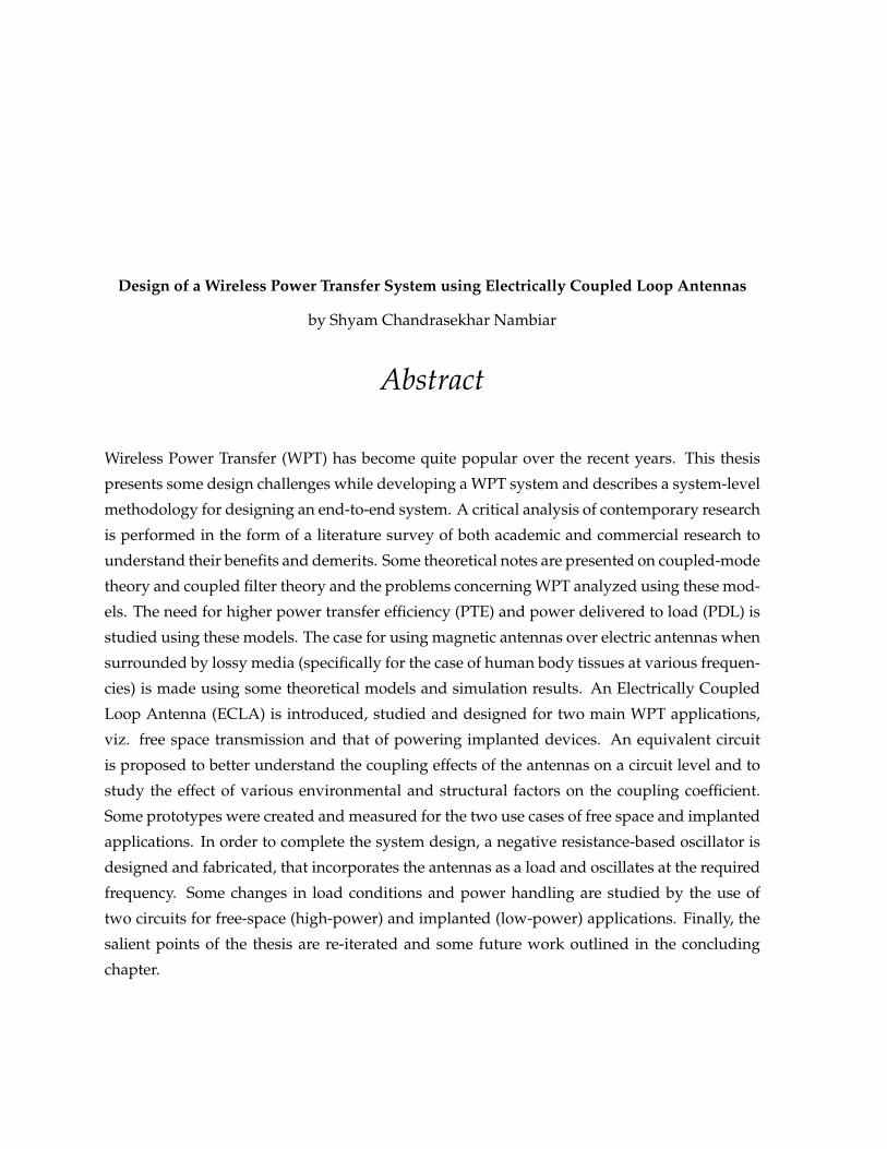
FIGURE 2.1: Overall system performance metrics
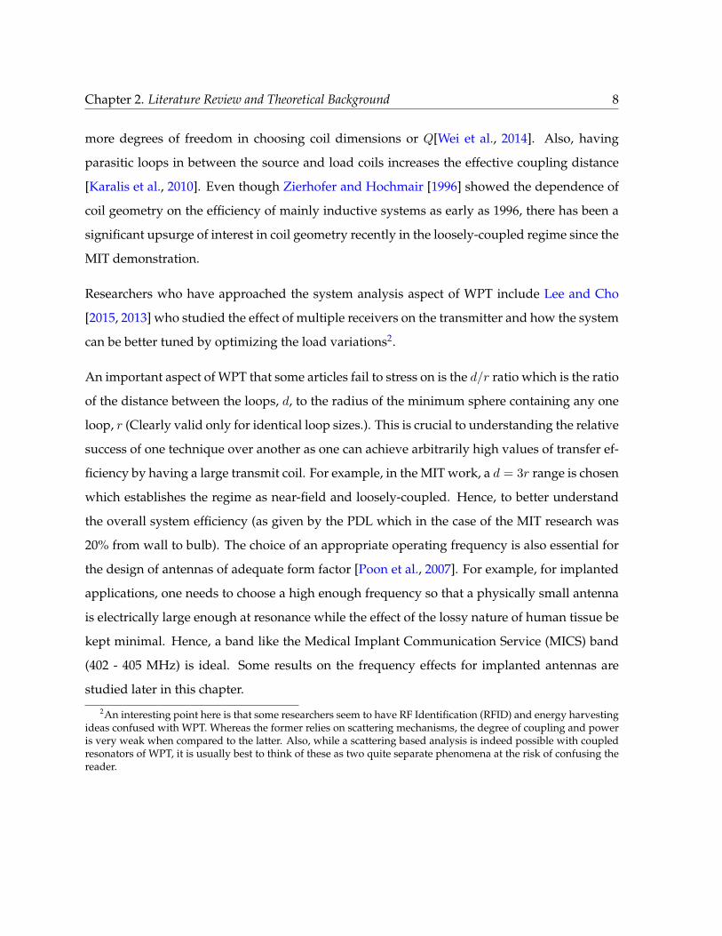
FIGURE 2.2: Coupled LC tank circuit system (Wei, X., Wang, Z., and Dai, H. (2014). A crit-ical review of wireless power transfer via strongly coupled magnetic resonances. Energies,
7(7):4316-4341. Used under fair use, 2015.)
2.1.2 Coupled-Mode Theory
The Coupled-Mode Theory (CMT) formalism is used extensively in opto-electronics, optical
guides and by physicists in general [Haus et al., 1984, Pollock, 1995]3. CMT is a perturbational
approach by which a coupled second-order differential equation can be decoupled to simpler
first-order equations by means of a complex amplitude term. In general, a mode can mean
many different things in physics, for example propagation modes, resonant or normal modes
of vibration, polarization states, etc.4. In the specific case of WPT analysis, it is easier to vi-
sualize the mode quantity as a resonant mode of an LC resonator[Haus et al., 1984]. Thus,
considering Fig. 2.2, we can define the following terms
3This is probably why it was the MIT researchers’ choice of analysis as they were physicists too.4http://emlab.utep.edu/ee5390em21/Lecture%205%20--%20Coupled-mode%20theory.pdf

Chapter 2. Literature Review and Theoretical Background 10
v = Ldi
dt(2.1)
i = −Cdvdt
(2.2)
d2v
dt2+ ω2
0v = 0 (2.3)
where
ω20 =
1
LC
Let a± be some complex amplitude such that
a± =
√C
2
(v ± j
√L
Ci
)(2.4)
da+
dt= jω0a+ (2.5)
da−dt
= −jω0a− (2.6)
Here, these amplitudes can be seen to hold the energy of the circuit when their magnitude
is squared (|a±|2 = W ). The ± subscript for amplitudes denotes the positive and negative
frequency components of the mode. Most discussions do not generally use the negative term
as it is just the complex conjugate of the positive term [Haus et al., 1984].
Also, Γ is used to denote the damping factor of the lossy resonators (and not the reflection
coefficient as in S-parameter analysis!), for both intrinsic and external loss/decay and is thus
tied to the Quality factor of the loops. For a lossy tank circuit, if unloaded Q is
Qunloaded =ω
2Γ=ωL
R
Chapter 2. Literature Review and Theoretical Background 11
then
Γ =R
2L
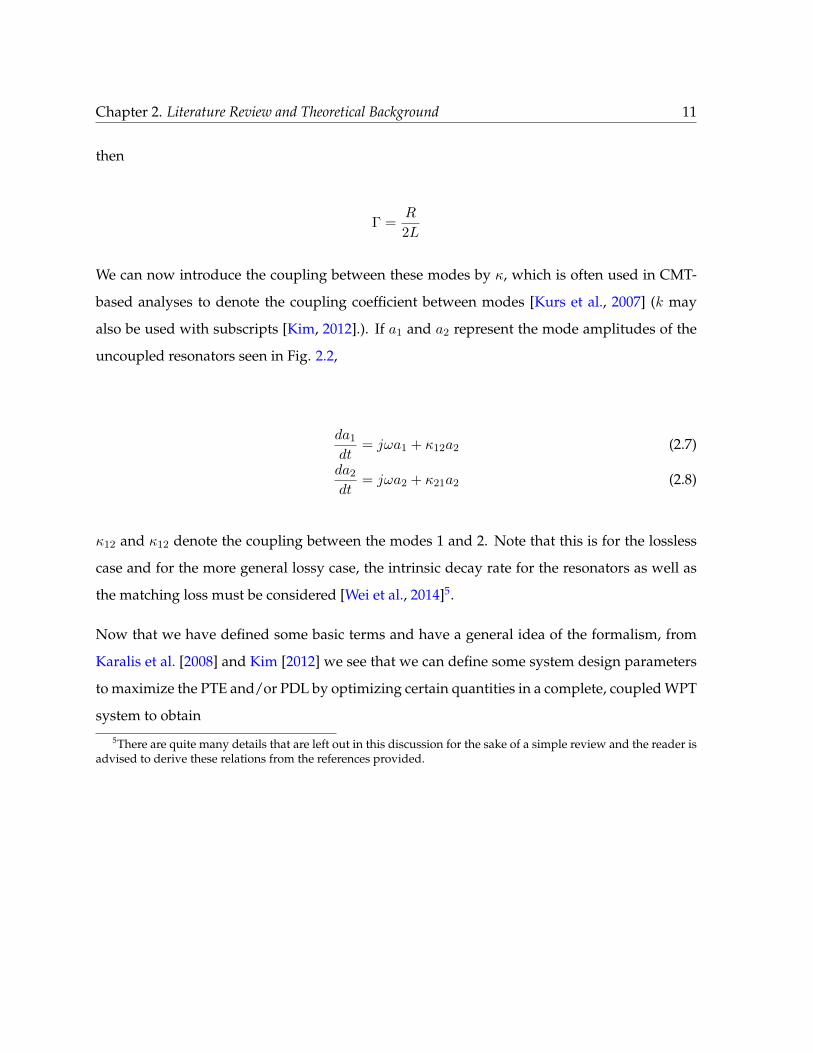
We can now introduce the coupling between these modes by κ, which is often used in CMT-
based analyses to denote the coupling coefficient between modes [Kurs et al., 2007] (k may
also be used with subscripts [Kim, 2012].). If a1 and a2 represent the mode amplitudes of the
uncoupled resonators seen in Fig. 2.2,
da1
dt= jωa1 + κ12a2 (2.7)
da2
dt= jωa2 + κ21a2 (2.8)
κ12 and κ12 denote the coupling between the modes 1 and 2. Note that this is for the lossless
case and for the more general lossy case, the intrinsic decay rate for the resonators as well as
the matching loss must be considered [Wei et al., 2014]5.
Now that we have defined some basic terms and have a general idea of the formalism, from
Karalis et al. [2008] and Kim [2012] we see that we can define some system design parameters
to maximize the PTE and/or PDL by optimizing certain quantities in a complete, coupled WPT
system to obtain
5There are quite many details that are left out in this discussion for the sake of a simple review and the reader isadvised to derive these relations from the references provided.
Chapter 2. Literature Review and Theoretical Background 12
U =κ√
Γ1Γ2= KU
√Q1Q2 (2.9)
where KU =M√L1L2
(2.10)
Uopt =√
1 + U2 (2.11)
ηopt =
(U
1 +√
1 + U2
)2
(2.12)
Here, U and KU are intermediate variables that are used in the optimization of the overall
transfer efficiency. Thus, the optimum efficiency (ηopt) is achieved when the above criterion
is achieved, which can be seen to be dependent on the quality factors of the coils. Due to
physical limitations, there is a need to equalize the source and load resistances to guarantee
optimal performance, failing which we are stuck with sub-optimal efficiency [Kim, 2012]. This
means that some sort of controllable input impedance network should be aimed for (which we
will design in the next few chapters). As discussed previously, more degrees of freedom are
obtained by increasing the number of loops in the system. It will be shown in Chapter 3 that
the value of coupling coefficient is very low for loosely coupled systems, and thus high-quality
factor loops are an implicit requirement for achieving high PTE. Also, it is possible to develop
an understanding for over, under, or critically-coupled resonators by looking at the value of U .
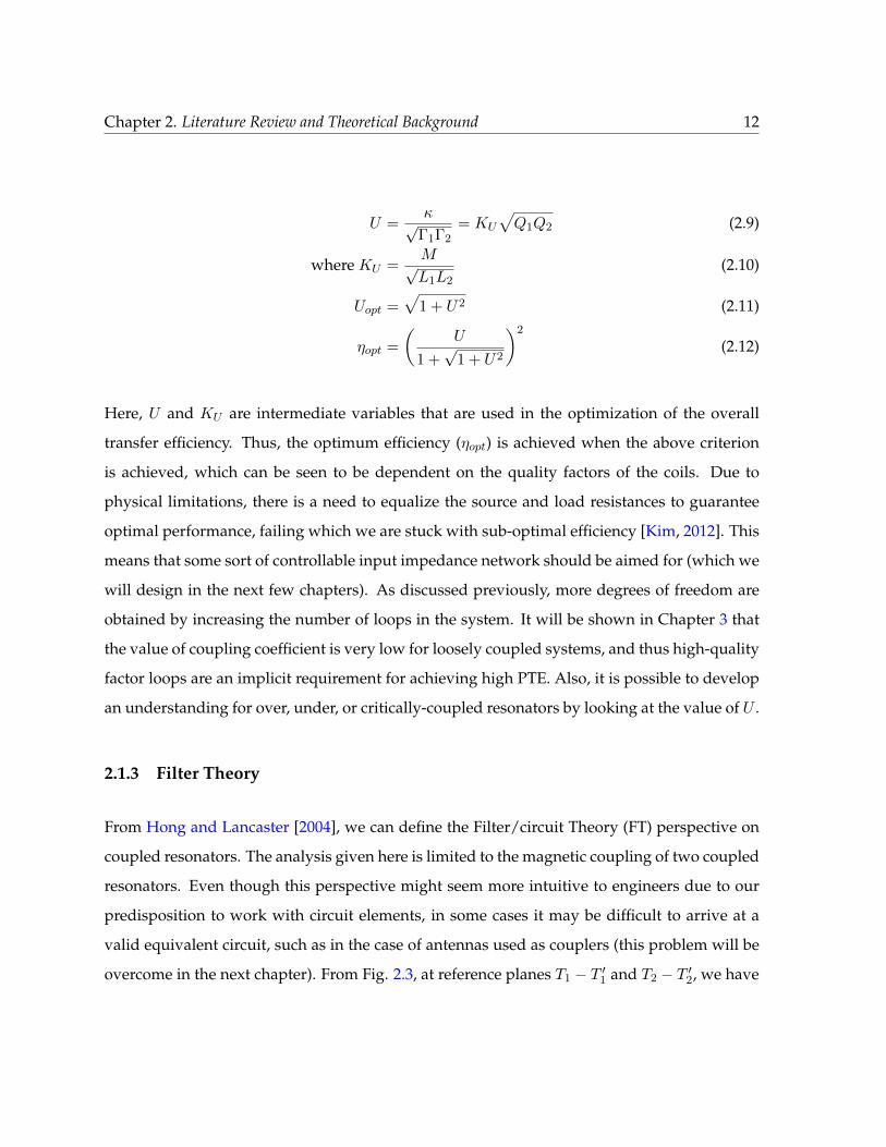
2.1.3 Filter Theory
From Hong and Lancaster [2004], we can define the Filter/circuit Theory (FT) perspective on
coupled resonators. The analysis given here is limited to the magnetic coupling of two coupled
resonators. Even though this perspective might seem more intuitive to engineers due to our
predisposition to work with circuit elements, in some cases it may be difficult to arrive at a
valid equivalent circuit, such as in the case of antennas used as couplers (this problem will be
overcome in the next chapter). From Fig. 2.3, at reference planes T1 − T ′1 and T2 − T ′2, we have
Chapter 2. Literature Review and Theoretical Background 13
FIGURE 2.3: Equivalent circuit for magnetically coupled resonators (Hong, J.-S. G. and Lan-caster, M. J. (2004). Microstrip filters for RF/microwave applications, volume 167. John Wiley
& Sons. Used under fair use, 2015.)
V1 = jωLI1 + jωLmI2 (2.13)
V2 = jωLI2 + jωLmI1 (2.14)
fe =1
2π√
(L− Lm)C(2.15)
fm =1
2π√
(L+ Lm)C(2.16)
where Lm is the mutual inductance and L,C are the equivalent inductance and capacitance
respectively when the resonator is self-resonant and isolated (decoupled). Also, fe, fm are the
frequencies due to the shift in the stored flux as given in Hong and Lancaster [2004] (Subscripts

Chapter 2. Literature Review and Theoretical Background 14
e and m represent the insertion of an electric/magnetic wall for analysis.). Then, the magnetic
coupling coefficient is given by
kM =f2e − f2
m
f2e + f2
m
=LmL
(2.17)
This may also be seen as the even and odd mode coupling as shown in Heebl et al. [2014], Kim
et al. [2010] where even and odd modes are considered to be the modes above and below the
resonant frequency in the isolated (non-coupled) case. Typically, this splitting is limited to the
strongly-coupled regime and both modes coalesce in the loosely-coupled regime.
Note that this is the case for synchronously tuned filters and that for the more general asyn-
chronous cases, this is but a degenerate case. From the formulation above, we can see that it is
possible to extract the coupling coefficient [Kim et al., 2010] and/or quality factor information
from coupled resonator system to study it further (using both magnitude and phase informa-
tion of S21). This is especially useful for implanted applications where the effect of the body
on the resonators is not quite clear or well understood.
2.1.4 Comparison
Useful side-by-side comparisons of the circuit-theoretic and the CMT approach are given in
Hui et al. [2013], Kiani and Ghovanloo [2012], Kim [2012]. Wei et al. [2014] bring out the state
of the art in terms of both theories and clearly demarcate which theory is better suited for the
application at hand while also discussing various system architectures. An interesting result
that follows from this analysis is that both approaches are perfectly valid ways of approach-
ing the problem with no perceived benefit of one over the other as long as the physics for the
assumptions (near-field conditions) hold true. It is important to realize that CMT is a pertur-
bational approach and that it is valid only when the first few modes are the most dominant,
which is the case for loosely coupled WPT systems. The circuit theory model, albeit simple
and straightforward, suffers from the problem of relying on fixed network parameters. For
Chapter 2. Literature Review and Theoretical Background 15
example, any change in the load network would require a re-work of the calculations which
may seem tedious and impractical for real-time applications (changing load conditions).
Azad et al. [2012] have achieved a Friis equation-like formulation for the near-field coupling
but the near-field equation here is a misnomer as the approach is still derived from an equiva-
lent circuit method. It is not truly from an antenna perspective. Although the objective of this
thesis is not to present a complete theoretical formulation for the near field behavior of the cou-
pling antennas, we will strive to analyze the system from an antenna perspective where and
when possible with possible segue into an equivalent circuit to understand the system from a
more established/conventional circuit perspective as well.
2.2 Overview of Industrial Standards
The main objective of this section is to understand contemporary commercial WPT schemes.
At 100 kHz, the Qi standard published by the Wireless Power Consortium (WPC) is a form of
non-resonant inductive coupling. Its specifications are maintained by the WPC (currently at
v1.1.2) and split into three possible regimes: Low, Medium and High power. Currently only
low power (5 W) exists in the market. Efforts are ongoing to realize medium power devices
(up to 120 W) commercially. High power operation has not been standardized yet. Qi includes
a communication protocol that enables WPT control by a mobile device. It requires low stand-
by power and has a typical operating distance of 5 mm for device size of about 40 mm. Other
such inductive methods include Duracell’s Powermat technology.
Qi is by far the most wide-spread of WPT schemes. It incorporates “foreign object detection”
which prevents heating of metal objects in the neighborhood of an active transmitter. Some
Qi-specific terms are given below.
Qi - Guided vs Free positioning
Guided Positioning - User must actively align the Secondary Coil to the Primary Coil, by
placing the Mobile Device on the appropriate location of the Interface Surface. The mobile
device provides an alignment aid that is appropriate to its size, shape and function.
Chapter 2. Literature Review and Theoretical Background 16
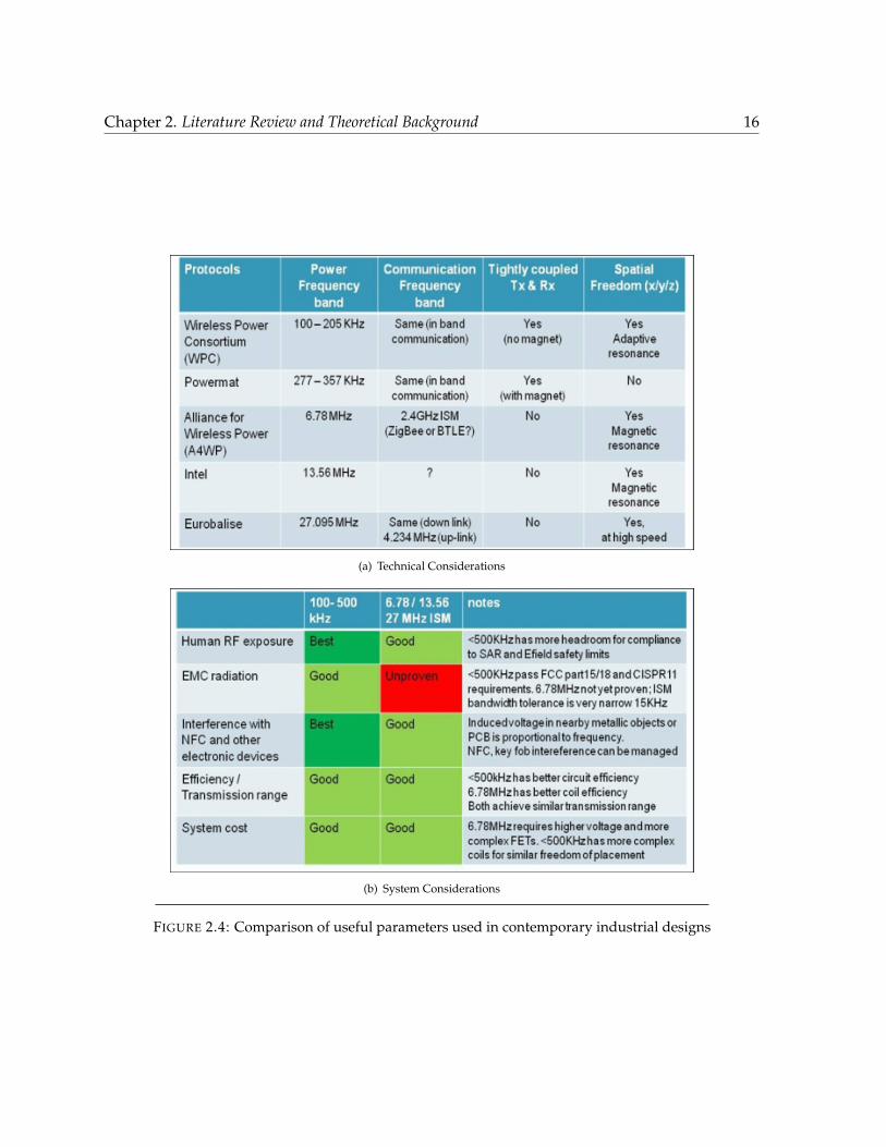
(a) Technical Considerations
(b) System Considerations
FIGURE 2.4: Comparison of useful parameters used in contemporary industrial designs
Chapter 2. Literature Review and Theoretical Background 17
Free Positioning - makes use of an array of Primary Coils to generate a magnetic field at the
location of the Secondary Coil only. Another implementation uses mechanical means to move
a single Primary Coil underneath the Secondary Coil.
Communication between transmit and receive coils takes place through a digital ping in Qi
which makes use of backscatter modulation (Differential bi-phase bit encoding like that used
in RFID systems)
Other WPT schemes include WiTricity6 which is based on the work by Karalis et al. [2008],
Kurs et al. [2007]. Competing technologies are Intel’s Wireless Resonant Energy Link (WREL)7
(operating at 13.56 MHz) and Alliance 4 Wireless Power’s (A4WP) Rezence technology (op-
erating at 6.78 MHz). On February 11 2014, A4WP and Power Matters Alliance (PMA) an-
nounced plans for co-operative growth and inter-operable standards. Fig. 2.48 gives an idea of
the relative pros and cons of each of this technologies and a qualitative idea of the suitability
of their operational frequencies for various purposes. Qualcomm has also been involved with
electric vehicle charging with its project called Halo (possible collaboration with Tesla Motors)
as well as other applications of WPT [Mohammadian, 2009, Toncich et al., 2009].
2.3 Implanted Antennas: Electric vs. Magnetic Antennas in Lossy
Media
Due to the steady rise in demand for implantable devices in recent years, the issue of power
transfer to these devices warrants a study into the suitability of certain antennas over others.
This problem is studied in this section where theoretical results are developed to promote the
candidacy of magnetic antennas over electric antennas specifically in the case of implanted
applications.
6http://www.witricity.com/assets/highly-resonant-power-transfer-kesler-witricity-2013.pdf
7http://newsroom.intel.com/docs/DOC-11198https://community.freescale.com/community/the-embedded-beat/blog/2012/11/30/
wireless-power-technology-comparison

Chapter 2. Literature Review and Theoretical Background 18
In this section, the near-field radiation characteristics of electric and magnetic antennas when
surrounded by a lossy dielectric medium are described. This study is relevant for cases such as
implanted antennas, submarine or underground communications where the antenna’s near-
field consists of lossy dielectric media such as human tissues, minerals or saline water. The-
oretical results for both types of small antennas are presented and expressions to show the
difference in stored energy and radiated power in the radian sphere [Wheeler, 1959] around
the antenna are formulated. These “ideal” results are then validated using simulation results
from a center-fed small dipole and a small loop antenna as a dual of magnetic dipole. It will
be shown that magnetic antennas give much better performance when surrounded by a lossy
dielectric9.
2.3.1 Overview and Motivation
The study of the near-field of antennas is of great significance in applications where the antenna
is located next to or inside a lossy medium because the medium properties can greatly alter
the performance of the antenna while themselves being subject to effects such as dielectric
heating and magnetization. This is typically the case for antennas near the human body [Kim
and Rahmat-Samii, 2004], soil [Large et al., 1973], submarine [Wheeler, 1958], or other lossy
media. In order to reduce the time-to-market, an antenna designer may choose a simple design;
however, this choice needs to take into consideration the nature of the surrounding medium.
It will be shown that antenna performance in a lossy medium is directly linked to whether it
has a dominant electric or magnetic field intensity in the near-zone. This study focuses on the
specific case of how antennas in implanted medical devices are affected by the presence of the
human body.
The demand for smart implanted medical devices has been growing exponentially during the
last few decades [Hall and Hao, 2006, Zimmerman, 1996]. Most modern implanted devices are
able to receive commands from the outside world or relay information from various sensors
within the host body. Thus, it can be seen that implanted antennas will play a significant role
9The material given in this section is incorporated from the paper by Manteghi and Ibraheem [2014] to whichthe author contributed.

Chapter 2. Literature Review and Theoretical Background 19
in the future of healthcare technology. However, there are many challenges involved in the
design of implanted antennas, including but not limited to: antenna miniaturization, antenna
loss due to miniaturization (structural loss), radiation loss that manifests itself in the immediate
near-field (environmental or near-field loss), compatibility with the human tissues, detuning,
etc. The goal of this study is to investigate losses that arise inside a conductive medium (such
as the human body) due to the strong reactive and radiating near-field for two main classes of
small antennas: electric antennas and magnetic antennas. Antennas in lossy media and near
material half-spaces have been studied in detail in King et al. [1981], Smith [1984] but the focus
here is on the use of electrically small antennas with highly reactive near fields specifically with
a focus on biomedical or implanted device applications.
Electrically Small Antennas
Previous research by Wheeler [Wheeler, 1947, 1975], Chu [Chu, 1948], Harrington [Harrington,
1960] and others [Collin and Rothschild, 1964, Davis et al., 2011, McLean, 1996] has focused on
the physical limitations of antennas with regard to size, gain, directivity, quality factor, and
the interdependence of these quantities. Karlsson [2004] and Wait [1952] have investigated
antennas surrounded by a lossy or conducting medium, but with a focus on finding optimal
values for antenna gain and radiation efficiency. To the best of the authors’ knowledge, a study
of the effect of the surrounding lossy media in the near-field based on the type of antenna has
not been conducted before. This issue, with a focus on electrically small antennas [Wheeler,
1975], is addressed at length in this study by computing the power loss and radiated power
for electric and magnetic antennas. Especially in the case of implanted devices, the power
lost in the near-field goes into heating human tissues which needs to comply with standards
set by government agencies. Through analytical expressions and simulations, the case for
magnetic antennas will be made by comparing the power dissipated in the lossy medium and
the radiated power for electric and magnetic antennas.
Chapter 2. Literature Review and Theoretical Background 20
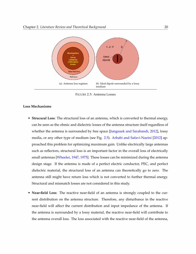
(a) Antenna loss regimes (b) Ideal dipole surrounded by a lossymedium
FIGURE 2.5: Antenna Losses
Loss Mechanisms
• Strucural Loss: The structural loss of an antenna, which is converted to thermal energy,
can be seen as the ohmic and dielectric losses of the antenna structure itself regardless of
whether the antenna is surrounded by free space [Jungsuek and Sarabandi, 2012], lossy
media, or any other type of medium (see Fig. 2.5). Arbabi and Safavi-Naeini [2012] ap-
proached this problem for optimizing maximum gain. Unlike electrically large antennas
such as reflectors, structural loss is an important factor in the overall loss of electrically
small antennas [Wheeler, 1947, 1975]. These losses can be minimized during the antenna
design stage. If the antenna is made of a perfect electric conductor, PEC, and perfect
dielectric material, the structural loss of an antenna can theoretically go to zero. The
antenna still might have return loss which is not converted to further thermal energy.
Structural and mismatch losses are not considered in this study.
• Near-field Loss: The reactive near-field of an antenna is strongly coupled to the cur-
rent distribution on the antenna structure. Therefore, any disturbance in the reactive
near-field will affect the current distribution and input impedance of the antenna. If
the antenna is surrounded by a lossy material, the reactive near-field will contribute to
the antenna overall loss. The loss associated with the reactive near-field of the antenna,

Chapter 2. Literature Review and Theoretical Background 21
which is converted to thermal energy in the surrounding material, is termed environ-
mental or near-field loss in this study. There are some limits on the amount of thermal
energy generated by an implanted transmitter which are set by regulatory bodies such as
the United States Federal Communications Commission (FCC) and the European Radio-
communications Committee (ERC) which is usually characterized by the term Specific
Absorption Rate or SAR. According to the FCC and ERC, the maximum limits for SAR
averaged over 1g and 10g of tissue mass are 1.6 W/kg [Federal Communications Com-
mission, 1996] and 2 W/kg, respectively [Commission, 1995]. The question is how does
the antenna type affect the total radiated power for a given antenna size while still sat-
isfying the FCC limits? Results of an investigation into this problem are studied in this
section of the thesis.
• Path Loss: It is well known that the radiated fields of any antenna in the far zone is a
locally plane wave. For a plane wave, the ratio of electric field to the magnetic field is
dictated by the material properties in the far-field and not the antenna type. However,
the ratio of total electric field to the total magnetic field in the reactive near zone of a
small antenna can vary from a very small number (0 for a magnetic point source at the
origin) to a very large number (infinity for an electric point source at the origin). Thus,
it is clear that the reactive near-field of a small antenna can vary dramatically from one
antenna type to another based on the radiation mechanism. Since the reactive near-field
of a small antenna is strongly coupled to the antenna structure, it is beneficial to define
antenna loss in the reactive near zone as an antenna-dependent environmental loss which
can be distinguished from the structural loss mentioned above. At the same time, one can
distinguish the near-field environmental loss from the path loss which usually deals with
plane waves (far-field) and will be independent of the antenna type.
2.3.2 Theoretical Results
For simplicity, two ideal dipoles (an electric dipole and a magnetic dipole) will be analyzed
in a homogeneous lossy medium with a finite conductivity (or dielectric loss). The exact total

Chapter 2. Literature Review and Theoretical Background 22
field of these two antennas can be found analytically, and therefore, one will be able to com-
pare their near-field stored energy, radiated power and dissipated power in the closed form.
This analysis allows us to study the behavior of small antennas in a lossy medium without
concerning ourselves with the antenna design, mismatch issues, and the antenna structural
loss. However, note that the approach used here is a perturbational method as the concept of
effect of the antenna size on near-zone fields is studied through a normalization of the power
flowing through an imaginary sphere (of varying size) and thus the results presented here are
an approximation of the expected performance.
• Ideal Dipoles
Consider a homogeneous medium with permittivity, permeability and conductivity of
ε, µ and σ respectively. An electric (or magnetic) dipole of length ∆z, carrying a uniform
current I (or K) in the z direction, is located at the origin. One can find the electric and
magnetic fields of these dipoles from Jin [2011] as
EE = j∆zµωIe−rγ
4πr3γ2
(2 (1 + rγ) cos (θ) r +
(1 + γr + γ2r2
)sin (θ) θ
)HE = ∆zI(1+rγ)e−rγ sin(θ)
4πr2φ
(2.18)
EM = ∆zK(1+rγ)e−rγ sin(θ)4πr2
φ
HM = j∆zKe−rγ
4πµωr3
(2 (1 + rγ) cos (θ) r +
(1 + γr + γ2r2
)sin (θ) θ
) (2.19)
where
γ = α+ jβ =√jωµ (jωε+ σ) (2.20)
Chapter 2. Literature Review and Theoretical Background 23
with
α = ω
√εµ
2
√−1 +
√1 +
σ2
ε2ω2(2.21a)
β = ω
√εµ
2
√1 +
√1 +
σ2
ε2ω2(2.21b)
The electric field intensity is proportional to the inverse of r2 for the magnetic dipole in
the near-zone while it is proportional to inverse of r3 for the electric dipole. It means that
E ·E∗ in the near-zone is proportional to 1/r4 and 1/r6 for magnetic and electric dipoles,
respectively. Therefore, the ohmic loss associated with conductance, σ, of the medium
will be higher for an electric dipole in comparison to a magnetic dipole.
In order to proceed with these calculations, the input impedances of the antennas need
to be found to be able to feed both antennas with the same amount of power. Since
the surrounding lossy dielectric loads the antennas in different fashions, the antenna
impedances will not be similar to its respective free space input impedance. At the same
time, a finite thickness for both dipole antennas would need to be included to avoid field
singularities, and consequently, numerical solutions are required to proceed. However,
there is an alternative way to compare the performance of these two antennas in a lossy
medium. To avoid impedance computation and field singularities, we assume that the
antenna is located in an imaginary small sphere of radius a that just encloses the antenna
and generates the same field distribution outside of that sphere as the ideal dipole in
a homogeneous medium (see Fig. 2.5). As mentioned previously, we omit the stored
energy and any loss inside the small sphere of radius a as it represents the antenna’s
structural loss, similar to the assumptions made by Chu [1948].
• Power lost inside a lossy sphere
The electromagnetic power lost in a homogeneous lossy dielectric spherical shell with an
inner radius of a and an outer radius of b is computed as
Chapter 2. Literature Review and Theoretical Background 24
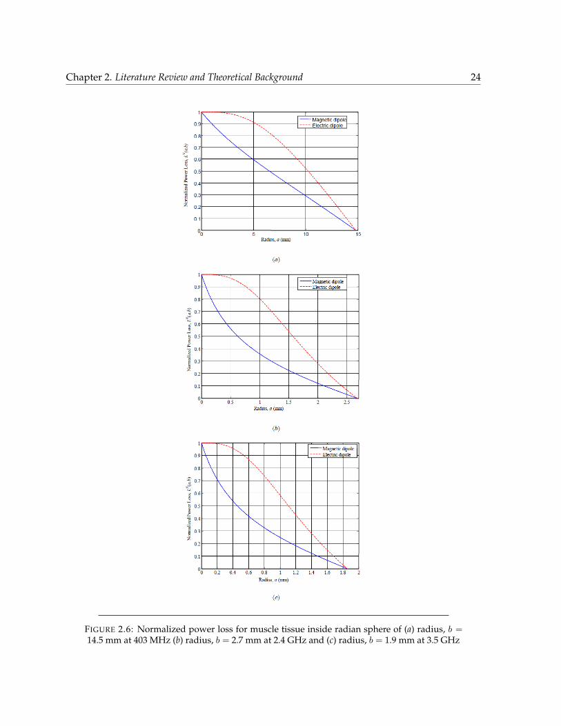
FIGURE 2.6: Normalized power loss for muscle tissue inside radian sphere of (a) radius, b =14.5 mm at 403 MHz (b) radius, b = 2.7 mm at 2.4 GHz and (c) radius, b = 1.9 mm at 3.5 GHz
Chapter 2. Literature Review and Theoretical Background 25
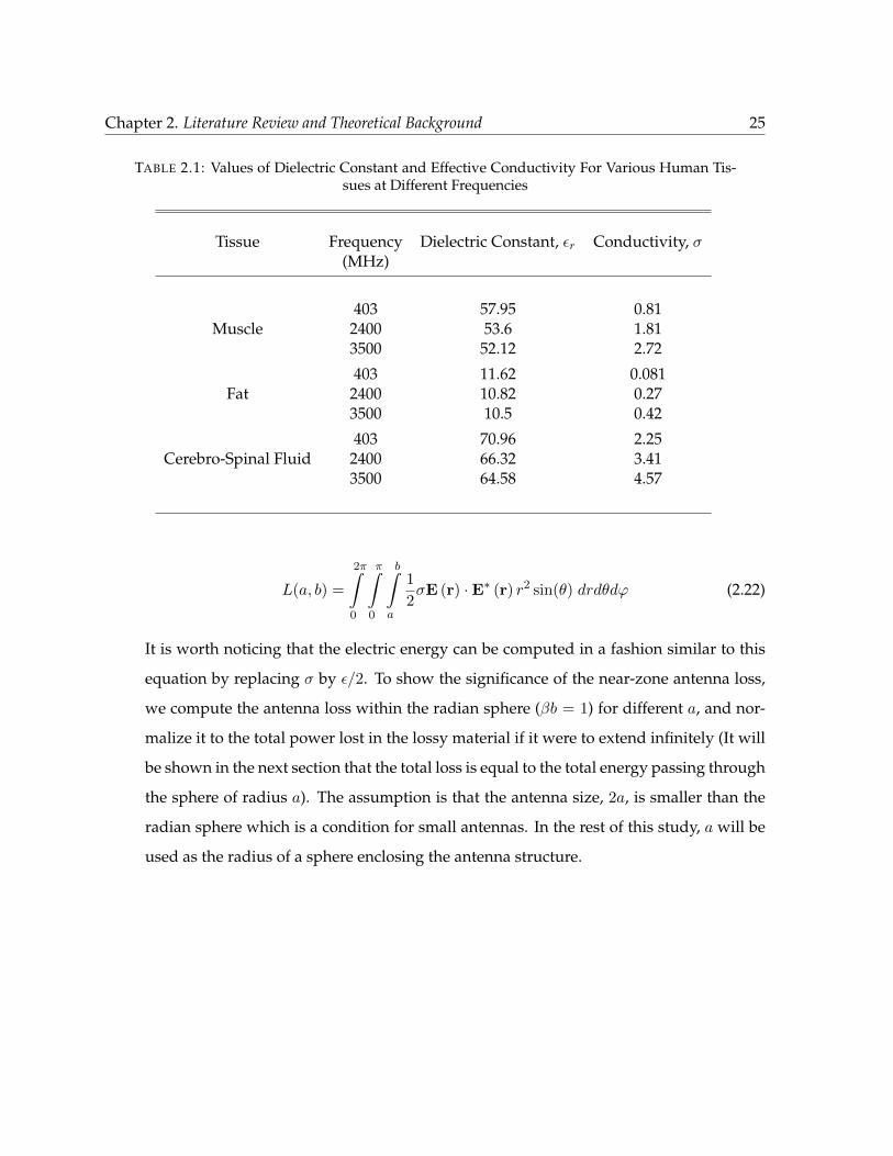
TABLE 2.1: Values of Dielectric Constant and Effective Conductivity For Various Human Tis-sues at Different Frequencies
Tissue Frequency Dielectric Constant, εr Conductivity, σ(MHz)
403 57.95 0.81Muscle 2400 53.6 1.81
3500 52.12 2.72
403 11.62 0.081Fat 2400 10.82 0.27
3500 10.5 0.42
403 70.96 2.25Cerebro-Spinal Fluid 2400 66.32 3.41
3500 64.58 4.57
L(a, b) =
2π∫0
π∫0
b∫a
1
2σE (r) ·E∗ (r) r2 sin(θ) drdθdϕ (2.22)
It is worth noticing that the electric energy can be computed in a fashion similar to this
equation by replacing σ by ε/2. To show the significance of the near-zone antenna loss,
we compute the antenna loss within the radian sphere (βb = 1) for different a, and nor-
malize it to the total power lost in the lossy material if it were to extend infinitely (It will
be shown in the next section that the total loss is equal to the total energy passing through
the sphere of radius a). The assumption is that the antenna size, 2a, is smaller than the
radian sphere which is a condition for small antennas. In the rest of this study, a will be
used as the radius of a sphere enclosing the antenna structure.

Chapter 2. Literature Review and Theoretical Background 26
The power lost for a magnetic dipole in a lossy medium from a to an arbitrary b is
LM (a, b) =∆z2|M |2σ
24πα
(e−2αa 2α+
(α2 + β2
)a
a− e−2αb 2α+
(α2 + β2
)b
b
)(2.23a)
'∆z2e−2αa|M |2σ
[2α+
(α2 + β2
)a]
24παa
∣∣∣∣∣b→∞
(2.23b)
Normalizing, we get
L(N)M (a, b) =
LM (a, b)
LM (a,∞)= 1−
ae−2(b−a)α(2α+
(α2 + β2
)b)
b (2α+ (α2 + β2) a)(2.24)
The power lost for an electric dipole in a lossy medium from a to arbitrary b is
LE (a, b) =∆z2|I|2µ2σω2e−2(a+b)α
24a3b3πα(α2 + β2)2 ×[b3e2bαf (α, β, a)− a3e2aαf (α, β, b)
](2.25a)
' ∆z2|I|2µ2σω2e−2αaf (α, β, a)
24πα(α2 + β2)2a3
∣∣∣∣∣b→∞
(2.25b)
Normalizing, we get
L(N)E (a, b) =
LE (a, b)
LE (a,∞)= 1− a3e−2(b−a)αf (α, β, b)
b3f (α, β, a)(2.26a)
wheref (α, β, r) = 2α+ 4α2r + 2α(α2 + β2
)r2 +
(α2 + β2
)2r3 (2.26b)
These normalized ratios are plotted in Fig. 2.6 for a typical muscle tissue at 403 MHz, 2.4
GHz and 3.5 GHz (see Table. 2.1 for material properties [Gabriel et al., 1996] as a function
of a for an electric dipole and a magnetic dipole in a radian sphere (b = 1/β) for each
frequency.
As Fig. 2.6(a) shows, almost 91% of the power is dissipated in the radian sphere (b = 14
mm) for the electric dipole with a = 5 mm (antenna size 10 mm). The same ratio is 60%

Chapter 2. Literature Review and Theoretical Background 27
for a magnetic antenna. It will be shown that outside of two radian spheres (b = 2/β), the
wave impedance approaches intrinsic impedance of the medium and the antenna type
does not affect the loss dramatically in this region.
• Radiated Power
In addition to the electromagnetic loss due to σ, the Poynting vector variations can also
be computed. One can find the real part of the radiated power passing through a sphere
of radius r as
P rad (r) =
2π∫0
π∫0
1
2Re [E×H∗] · rr2 sin (θ) dθdϕ (2.27)
The total radiated power of these antennas would be equal for a lossless medium (σ = 0)
if
M = ηI (2.28)
where η is the intrinsic impedance of the lossy material in which the antenna is placed.
To compare the radiation performance of ideal electric and magnetic dipoles in a lossy
material, one can compute the real part of the radiated power passing through a sphere
of radius r as
P radM (r) =∆z2e−2αr|M |2β
[2α+
(α2 + β2
)r]
12πrµω(2.29)
'∆z2e−2αr|M |2β
(α2 + β2
)12πµω
∣∣∣∣∣r→∞
(2.30)
P radE (r) =∆z2e−2αr|I|2βµω12πr3(α2 + β2)2 f (α, β, r) ' ∆z2e−2αr|I|2βµω
12π
∣∣∣∣∣r→∞
(2.31)

Chapter 2. Literature Review and Theoretical Background 28
In order to make a fair comparison between these two antennas, the radiated power
needs to be normalized to the input power. As we ignore the effects of structural and
mismatch losses in this study, we will define input power as the total real power that
passes through a sphere of radius a. As the medium in which the antenna resides is
lossy, the entire input power will be absorbed when b→∞ (i.e. the far-field).
P(N)M (r, a) =
P radM (r)
P radM (a)=
e−2α(r−a)a[2α+
(α2 + β2
)r]
r [2α+ (α2 + β2) a](2.32)
P(N)E (r, a) =
P radE (r)
P radE (a)=
e−2α(r−a)a3f (α, β, r)
r3f (α, β, a)(2.33)
where
P radM (a) = LM (a,∞) and P radE (a) = LE (a,∞)
Equations 2.32 and 2.33 provide the total radiated power passing through a sphere of ra-
dius r normalized to the input power for magnetic and electric ideal dipoles, respectively.
The normalized power is plotted versus a and distance r for a lossy dielectric mimicking
muscle at 403 MHz (with material properties seen in Table. 2.1) in Fig. 2.7. The radian
sphere has a radius of b = 14 mm at this frequency.
Fig. 2.7 demonstrates the superior performance of a magnetic antenna in comparison to
an electric antenna with the same size and the same input power. It can be observed from
these two figures that the difference between these two antennas is greater for a smaller
antenna size.
The ratio of the normalized power of these two antennas for different a will provide a
measure to compare the behavior of an ideal magnetic dipole to an ideal electric dipole
versus frequency, material loss, and antenna size.
P(N)M (r, a)
P(N)E (r, a)
=r2f (α, β, a)
[2α+
(α2 + β2
)r]
a2f (α, β, r) [2α+ (α2 + β2) a](2.34)
Chapter 2. Literature Review and Theoretical Background 29
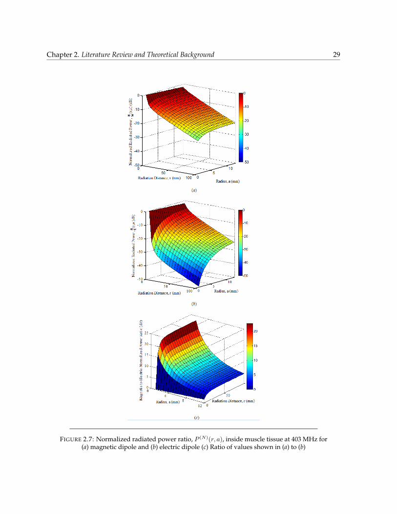
FIGURE 2.7: Normalized radiated power ratio, P (N)(r, a), inside muscle tissue at 403 MHz for(a) magnetic dipole and (b) electric dipole (c) Ratio of values shown in (a) to (b)
Chapter 2. Literature Review and Theoretical Background 30
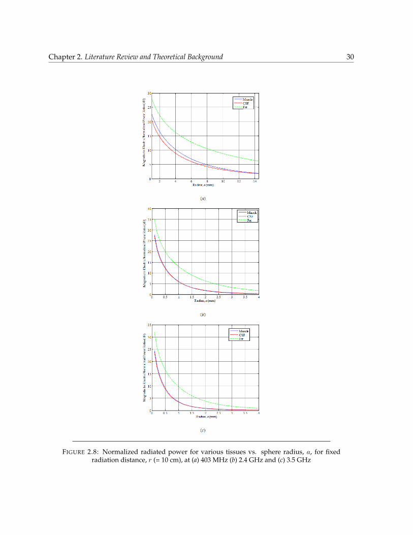
FIGURE 2.8: Normalized radiated power for various tissues vs. sphere radius, a, for fixedradiation distance, r (= 10 cm), at (a) 403 MHz (b) 2.4 GHz and (c) 3.5 GHz
Chapter 2. Literature Review and Theoretical Background 31
Fig. 2.7-c demonstrates this ratio at 403 MHz for implanted antennas inside a medium
mimicking muscle tissue. As it can be seen here, the ratio converges to a steady value
for an antenna size larger than two radian spheres. Fig. 2.8 shows this ratio for a fixed
r (= 10 cm) and varying a. This ratio has been plotted versus antenna size for three
different frequencies (403 MHz, 2.4 GHz and 3.5 GHz) when the antenna is located in
typical muscle tissue, fat tissue and Cerebrospinal Fluid (CSF) (see Table. 2.1) in Fig. 2.8.
The ratio of the normalized radiated power from a magnetic antenna to an electric an-
tenna in the far-zone simplifies to
limr→∞
(P
(N)M (r, a)
P(N)E (r, a)
)= 1 +
2α (1 + 2αa)
(α2 + β2) a2 (2α+ (α2 + β2) a)(2.35)
This shows that the radiated power from an ideal magnetic dipole is always more than
the radiated power from an ideal electric dipole with the same size for the same accepted
power in a medium with ohmic loss. This equation also shows that when the antenna
size become smaller, the magnetic antenna radiates much more effectively (1/a2 times
higher radiated power) than the electric dipole. Plotting either 2.34 for r a, or plotting
2.35 results in the same curves.
2.3.3 Simulation in FEKO
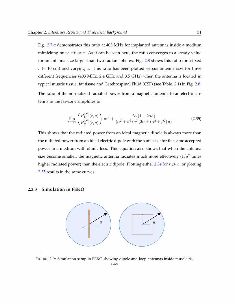
FIGURE 2.9: Simulation setup in FEKO showing dipole and loop antennas inside muscle tis-sues

Chapter 2. Literature Review and Theoretical Background 32
In order to validate the theoretical results using full-wave simulations, a dipole antenna (elec-
tric field antenna) with a length of 0.5 mm and a rectangular loop antenna (magnetic field
antenna) with the length of its diagonal as 0.5 mm were simulated using FEKO as shown in
Fig. 2.9. These sizes are chosen in order to ensure an electrically small antenna. These antennas
are surrounded by a homogeneous medium that has properties of a lossy dielectric mimicking
human muscle tissue at 403 MHz (see Table. 2.1 for tissue properties). Here, a is the radius
of the sphere enclosing the antenna as discussed previously and this sphere can be assumed
to be the antenna size. To remove the effects of any structural or mismatch loss from these
computations, the total radiated power passing through an imaginary sphere of radius a is
considered to be the total input power to the antenna (similar to the input power computation
for the theoretical formulation) while keeping the size of the physical antennas the same (so
as to ensure that the electrically small antenna criterion is met as well as to prevent excitation
of higher order modes in a larger antenna). The sphere radius a was varied from 1 mm to
14 mm in order to bring about a comparison with the theoretical results. The total radiated
power at various distances from r = a to a maximum distance of r = 100 mm is computed for
both antennas and it is normalized to the input power (power at r = a). Then the ratio of the
normalized radiated power for both antennas is computed for different radii of the imaginary
sphere (which is considered to represent the antenna size).
Since FEKO contains a Method of Moments (MoM) solver, solving for the fields for a antenna
surrounded by a lossy material is as easy as changing the free-space values of ε and µ10. A
similar approach in HFSS was tried by a colleague using the Volume Integration of Power
through the Fields Calculator function. However, this method yielded poor results possibly
due to the fact that the lossiness of the surrounding medium loaded the antenna under test
(AUT) adversely.
The flowchart of activities performed to extract the information from FEKO and post-processing
in MATLAB is shown in Fig. 2.10. A spherical near-field pattern was simulated for all the sim-
ulations. The resolution and limits of the data are manipulated prior to displaying the plots in
10The author would like to thank Dr. Davis for his help in setting up the simulation in FEKO
Chapter 2. Literature Review and Theoretical Background 33
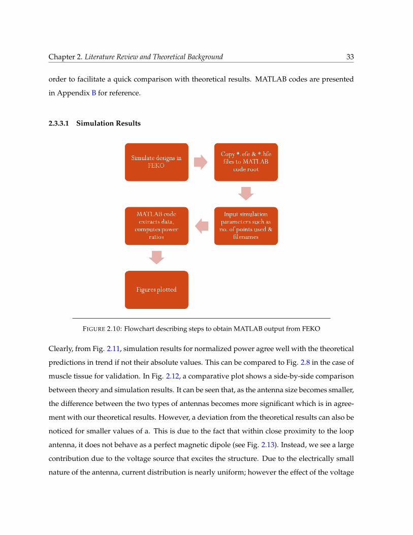
order to facilitate a quick comparison with theoretical results. MATLAB codes are presented
in Appendix B for reference.
2.3.3.1 Simulation Results
FIGURE 2.10: Flowchart describing steps to obtain MATLAB output from FEKO
Clearly, from Fig. 2.11, simulation results for normalized power agree well with the theoretical
predictions in trend if not their absolute values. This can be compared to Fig. 2.8 in the case of
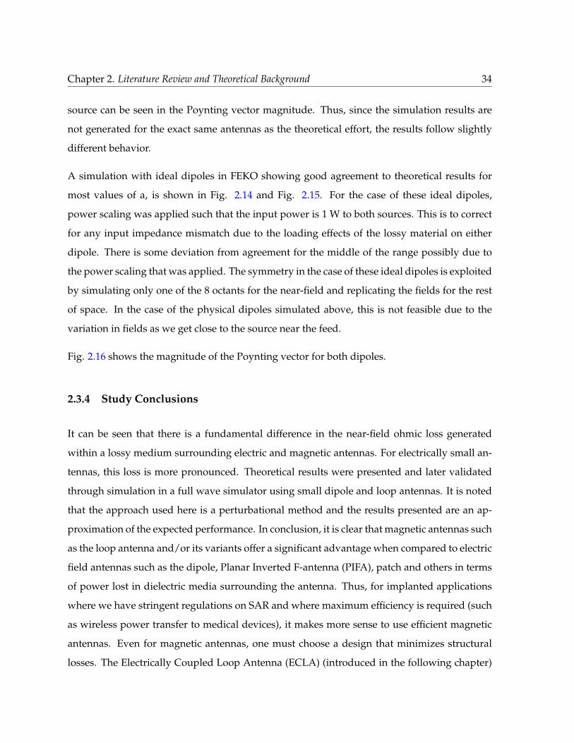
muscle tissue for validation. In Fig. 2.12, a comparative plot shows a side-by-side comparison
between theory and simulation results. It can be seen that, as the antenna size becomes smaller,
the difference between the two types of antennas becomes more significant which is in agree-
ment with our theoretical results. However, a deviation from the theoretical results can also be
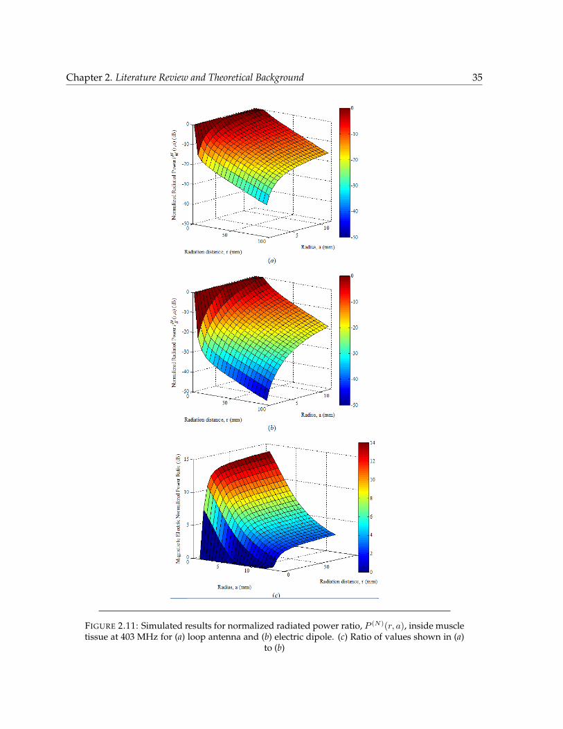
noticed for smaller values of a. This is due to the fact that within close proximity to the loop
antenna, it does not behave as a perfect magnetic dipole (see Fig. 2.13). Instead, we see a large
contribution due to the voltage source that excites the structure. Due to the electrically small
nature of the antenna, current distribution is nearly uniform; however the effect of the voltage
Chapter 2. Literature Review and Theoretical Background 34
source can be seen in the Poynting vector magnitude. Thus, since the simulation results are
not generated for the exact same antennas as the theoretical effort, the results follow slightly
different behavior.
A simulation with ideal dipoles in FEKO showing good agreement to theoretical results for
most values of a, is shown in Fig. 2.14 and Fig. 2.15. For the case of these ideal dipoles,
power scaling was applied such that the input power is 1 W to both sources. This is to correct
for any input impedance mismatch due to the loading effects of the lossy material on either
dipole. There is some deviation from agreement for the middle of the range possibly due to
the power scaling that was applied. The symmetry in the case of these ideal dipoles is exploited
by simulating only one of the 8 octants for the near-field and replicating the fields for the rest
of space. In the case of the physical dipoles simulated above, this is not feasible due to the
variation in fields as we get close to the source near the feed.
Fig. 2.16 shows the magnitude of the Poynting vector for both dipoles.
2.3.4 Study Conclusions
It can be seen that there is a fundamental difference in the near-field ohmic loss generated
within a lossy medium surrounding electric and magnetic antennas. For electrically small an-
tennas, this loss is more pronounced. Theoretical results were presented and later validated
through simulation in a full wave simulator using small dipole and loop antennas. It is noted
that the approach used here is a perturbational method and the results presented are an ap-
proximation of the expected performance. In conclusion, it is clear that magnetic antennas such
as the loop antenna and/or its variants offer a significant advantage when compared to electric
field antennas such as the dipole, Planar Inverted F-antenna (PIFA), patch and others in terms
of power lost in dielectric media surrounding the antenna. Thus, for implanted applications
where we have stringent regulations on SAR and where maximum efficiency is required (such
as wireless power transfer to medical devices), it makes more sense to use efficient magnetic
antennas. Even for magnetic antennas, one must choose a design that minimizes structural
losses. The Electrically Coupled Loop Antenna (ECLA) (introduced in the following chapter)
Chapter 2. Literature Review and Theoretical Background 35
FIGURE 2.11: Simulated results for normalized radiated power ratio, P (N)(r, a), inside muscletissue at 403 MHz for (a) loop antenna and (b) electric dipole. (c) Ratio of values shown in (a)
to (b)
Chapter 2. Literature Review and Theoretical Background 36
FIGURE 2.12: Comparison between theoretical and simulated results for normalized radiatedpower ratio, P (N)(r, a), inside muscle tissue at 403 MHz at r = 10 cm
FIGURE 2.13: Total Poynting vector magnitude (in dB W/m2) and Current Distribution on theelectrically small loop antenna
Chapter 2. Literature Review and Theoretical Background 37
(a) (b)
(c)
FIGURE 2.14: Simulated results for normalized radiated power ratio, P (N)(r, a), inside muscletissue at 403 MHz for (a) ideal magnetic and (b) ideal electric dipoles. (c) Ratio of values shown
in (a) to (b)
is a good candidate then by virtue of its high-Q resonator nature that can be conveniently
engineered to suit different applications.
Chapter 2. Literature Review and Theoretical Background 38
FIGURE 2.15: Comparison between theoretical and simulated results for normalized radiatedpower ratio, P (N)(r, a), inside muscle tissue at 403 MHz at r = 10 cm for ideal electric and
magnetic dipoles
(a) Ideal Magnetic Dipole (b) Ideal Electric Dipole
FIGURE 2.16: Magnitude of Poynting Vector for Ideal Dipoles
Chapter 3
Antenna Design
3.1 Introduction
The previous chapter established the different perspectives on design methodology that are
prevalent today in academia and the industry. It was seen that a vast majority of designs
approach the problem of Wireless Power Transfer (WPT) from the perspective of coupled coils.
While this is a perfectly reasonable way of analysis, some more insight into the problem may be
gleaned by exploring the design of a WPT system by using antenna theory. In this chapter, we
will focus on the use of antennas, namely their near-field, miniaturization for use in implanted
applications and the challenges associated with doing so.
It is clear that we require an antenna that can provide a close resemblance to the magnetic
dipole in the sense that we require strong magnetic coupling in the near-field. However, we
also require a high-Q antenna to be able to store this energy effectively around the antenna and
not let it radiate away. From the previous chapter’s discussion, we see that a high-Q antenna
will also help improve Power Transfer Efficiency (PTE) in a loosely coupled system. Thus,
an Electrically Coupled Loop Antenna (ECLA) is proposed [Manteghi, 2013b, Nambiar and
Manteghi, 2014a] in this chapter that acts as a high-Q resonator and can be used as a coupling
element for WPT systems. After studying the ECLA in some detail, an equivalent circuit is
39

Chapter 3. Antenna Design 40
presented followed by some simulation and measurement results for various use cases. As
discussed previously, the focus will be to realize two systems that fulfill two use cases, namely
a low frequency version that is suitable for commercial applications (target frequency of 13.56
MHz in the ISM band) in free space and a miniaturized version for implanted applications
(target frequency of 403 MHz in the MICS band).
3.2 Electrically Coupled Loop Antenna
The Electrically Coupled Loop Antenna (ECLA) was proposed in Manteghi [2013a] as a dual
for the Planar Inverted F-Antenna (PIFA) [Taga and Tsunekawa, 1987]. The PIFA, being an
electric antenna and characterized as a patch antenna with a shorting pin to reduce its size and
make the patch resonant, is a magnetic current antenna [Villamil and Manteghi, 2013]. There
are specific use cases where the qualities of the PIFA are better suited for a certain application
(such as cellphones which require small sized antennas and wide bandwidths). However, the
case for using the ECLA as a WPT candidate will be made in this thesis. The structure of a sim-
ple ECLA is shown in Fig. 3.1. It is basically a loop antenna that is coupled to the transmission
line through a capacitive feed. The distributed nature of the inductance and the capacitance
are responsible for the very high Q. It is also a self-matched antenna, where the dimensions of
the antenna’s capacitive “feed head” can be modified to control the input impedance of the an-
tenna and match it to a larger variation in transmission line impedance by choosing a suitable
feed head dimension and/or height (tp, ts). This capability for absorption of the impedance
into a high-Q resonator without the use of lumped components helps in lowering the loss in-
curred in the matching circuits required in other types of loops used for WPT. Also, the fact
that the ECLA is an electrically small antenna reduces its radiation efficiency and makes it less
susceptible to incur radiation losses; something that we would like to keep at a minimum in
non-radiative WPT (see Fig. 3.2). By virtue of its smaller physical size to achieve self-resonance,
the ECLA’s form factor is much smaller compared to some other loops. Additional coils to in-
crease Q are not required either to increase the Q of the system [Kiani and Ghovanloo, 2013,
Kiani et al., 2011] nor to achieve better matching [Karalis et al., 2008] (controlled entirely by
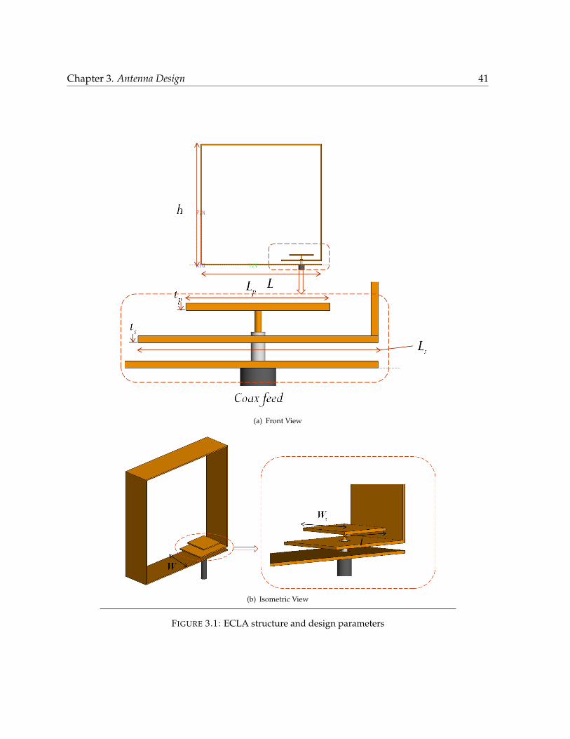
Chapter 3. Antenna Design 41
(a) Front View
(b) Isometric View
FIGURE 3.1: ECLA structure and design parameters

Chapter 3. Antenna Design 42
the ECLA’s feed head dimensions as shown in Table. 3.1). Moreover, due to the ECLA being a
magnetic field antenna in the near field, it is well suited for implanted applications (as shown
in 2.3).
TABLE 3.1: Control of Frequency Response using ECLA’s Design Parameters
Design variable Affected parameter
L, h Coarse control of resonant frequencyLs, ts,Ws,W Finer control of resonant frequency
Lp, tp Controls the Input Impedance
From Fig. 3.1, it can be seen that the resonance of the antenna can be controlled by tuning
the parameters shown in Table. 3.1. A design exploiting the frequency dependence of the
distributed capacitors for the purpose of miniaturization of the antenna will be discussed in
subsequent sections.
3.2.1 Antenna Characteristics
The ECLA has the characteristic “donut”-shaped far-field radiation pattern of a magnetic dipole
oriented along the X-axis as seen in Fig. 3.2. Also note that the far-field gain has a maximum
of -11.2 dBi at 13.95 MHz (Return Loss of 12 dB). A comparison of the near field distribution of
the total electric and magnetic field intensities is shown in Fig. 3.3 as well. Note that the values
are shown in dB scale to bring out the variation with r more clearly. At the resonant frequency,
the wavelength, λ = 21.5 m and ka = λ/2π = 3.4 m. Clearly, it can be seen that the ECLA is a
magnetic antenna with a relatively strong magnetic field in its near zone. Another method for
measuring antenna efficiency is the Wheeler cap method introduced in Wheeler [1959]1.
1http://www.rfcafe.com/references/articles/Efficiency-Measurement-Antenna-Wheeler-Cap.htm
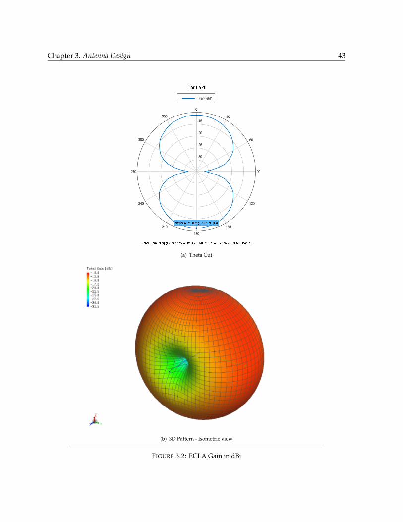
Chapter 3. Antenna Design 43
e
e
e
e
(a) Theta Cut
(b) 3D Pattern - Isometric view
FIGURE 3.2: ECLA Gain in dBi
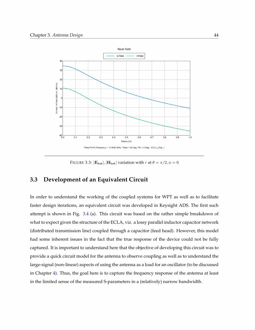
Chapter 3. Antenna Design 44
FIGURE 3.3: |Etot|, |Htot| variation with r at θ = π/2, φ = 0
3.3 Development of an Equivalent Circuit
In order to understand the working of the coupled systems for WPT as well as to facilitate
faster design iterations, an equivalent circuit was developed in Keysight ADS. The first such
attempt is shown in Fig. 3.4 (a). This circuit was based on the rather simple breakdown of
what to expect given the structure of the ECLA, viz. a lossy parallel inductor capacitor network
(distributed transmission line) coupled through a capacitor (feed head). However, this model
had some inherent issues in the fact that the true response of the device could not be fully
captured. It is important to understand here that the objective of developing this circuit was to
provide a quick circuit model for the antenna to observe coupling as well as to understand the
large-signal (non-linear) aspects of using the antenna as a load for an oscillator (to be discussed
in Chapter 4). Thus, the goal here is to capture the frequency response of the antenna at least
in the limited sense of the measured S-parameters in a (relatively) narrow bandwidth.
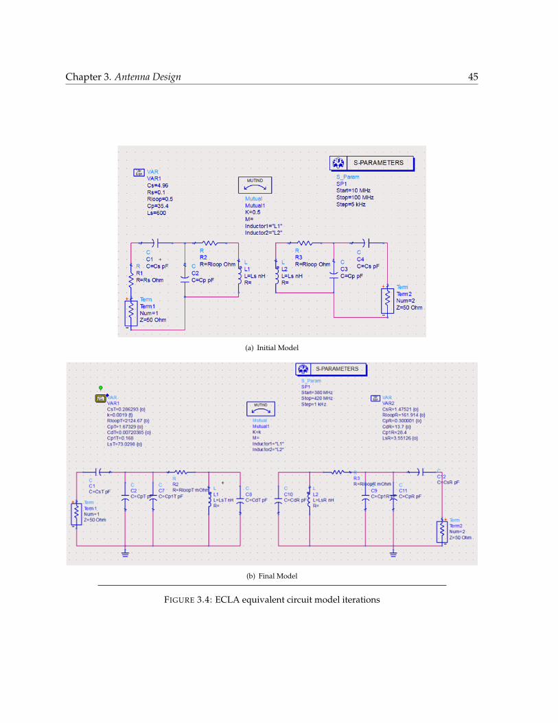
Chapter 3. Antenna Design 45
(a) Initial Model
(b) Final Model
FIGURE 3.4: ECLA equivalent circuit model iterations
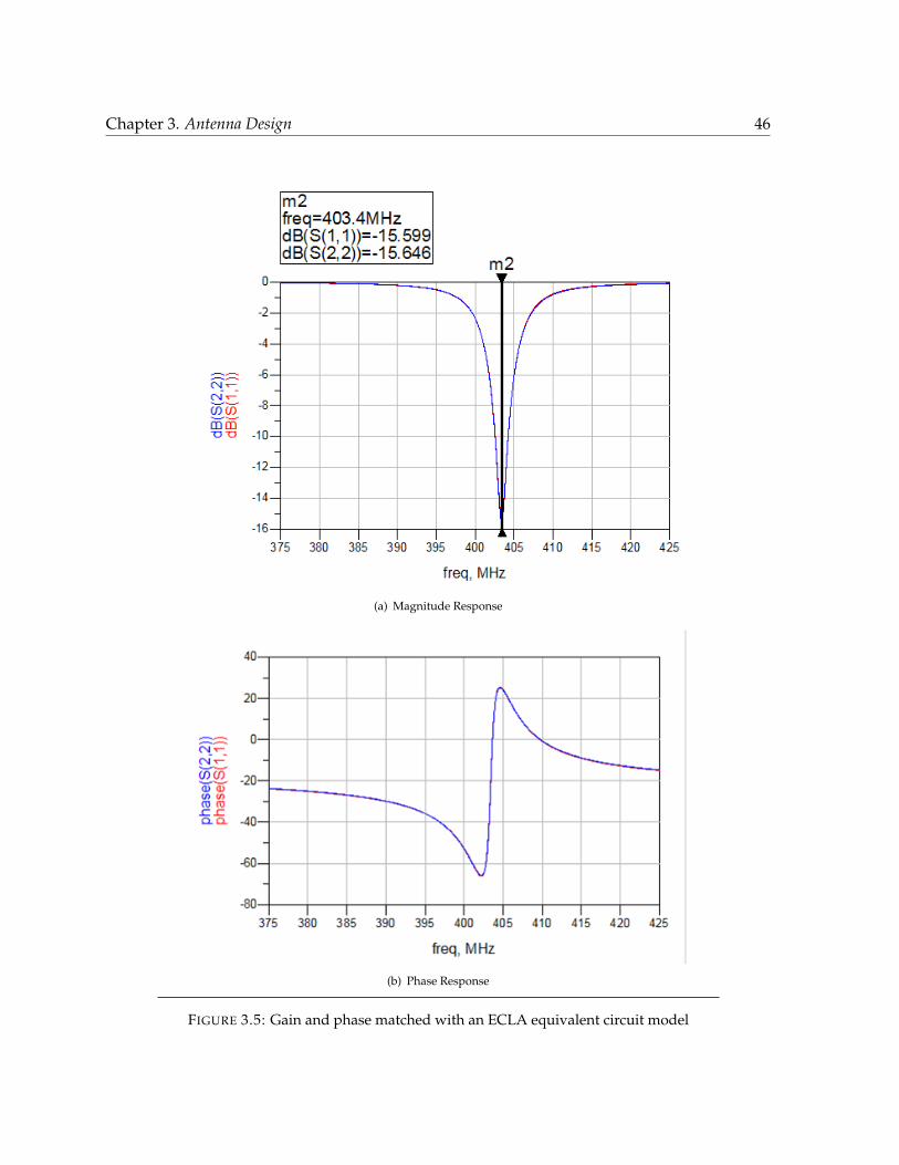
Chapter 3. Antenna Design 46
(a) Magnitude Response
(b) Phase Response
FIGURE 3.5: Gain and phase matched with an ECLA equivalent circuit model

Chapter 3. Antenna Design 47
Fig. 3.4 (b) was the result of combining a test bench setup in ADS where either the full-wave
or measured S-parameters of the AUT would be subject to an optimization process after initial
tuning (or “seeding”). For example, an approximate value for the feeding capacitors and loop
resistance can be calculated (on the first order, without accounting for fringing effects) using
standard parallel plate capacitor equations and skin depth calculations respectively. Also note
that a parallel capacitor was added across the inductor to achieve the required match. The
optimization flowchart and setup is explained in Appendix B.
Fig. 3.5 shows the result of the optimization process when applied to an ECLA for the MICS
band at 403 MHz. This technique will be used in the rest of the thesis for multiple applications.
3.4 ECLA Variants and Design Iterations
This section will discuss the design and simulation of some ECLA designs. Due to the ease of
its construction, a square ECLA formed from thin Copper sheet metal (of approximate thick-
ness 0.5 mm) was used for most initial designs. However, to obtain better current distribution
throughout the antenna, a circular ECLA was also prototyped using hollow brass or copper
tubing (discussed in the next section).
It should be noted that both the bottom capacitor and feed head dimensions need to be modi-
fied while manipulating the frequency as a particular feed head dimension that ensures a good
match at one frequency does not guarantee a match another frequency, say 5 MHz away. Some
hybrid design techniques using a combination of full-wave data and circuit-level simulation is
used to achieve faster design turnaround times.
We will also discuss the practical aspects of prototyping and measuring some ECLA designs2.
The following sections elaborate efforts to design and demonstrate WPT with ECLAs for dif-
ferent frequency bands and applications.
2The author would like to thank Dr. Manteghi, the staff of the Industrial and Systems Engineering Workshopin Whittemore Hall and the Virginia Tech Antenna Group’s Antenna Lab for their time and generous help whileusing their equipment.
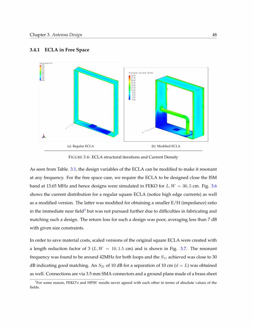
Chapter 3. Antenna Design 48
3.4.1 ECLA in Free Space
(a) Regular ECLA (b) Modified ECLA
FIGURE 3.6: ECLA structural iterations and Current Density
As seen from Table. 3.1, the design variables of the ECLA can be modified to make it resonant
at any frequency. For the free space case, we require the ECLA to be designed close the ISM
band at 13.65 MHz and hence designs were simulated in FEKO for L,W = 30, 5 cm. Fig. 3.6
shows the current distribution for a regular square ECLA (notice high edge currents) as well
as a modified version. The latter was modified for obtaining a smaller E/H (impedance) ratio
in the immediate near field3 but was not pursued further due to difficulties in fabricating and
matching such a design. The return loss for such a design was poor, averaging less than 7 dB
with given size constraints.
In order to save material costs, scaled versions of the original square ECLA were created with
a length reduction factor of 3 (L,W = 10, 1.5 cm) and is shown in Fig. 3.7. The resonant
frequency was found to be around 42MHz for both loops and the S11 achieved was close to 30
dB indicating good matching. An S21 of 10 dB for a separation of 10 cm (d = L) was obtained
as well. Connections are via 3.5 mm SMA connectors and a ground plane made of a brass sheet
3For some reason, FEKO’s and HFSS’ results never agreed with each other in terms of absolute values of thefields.
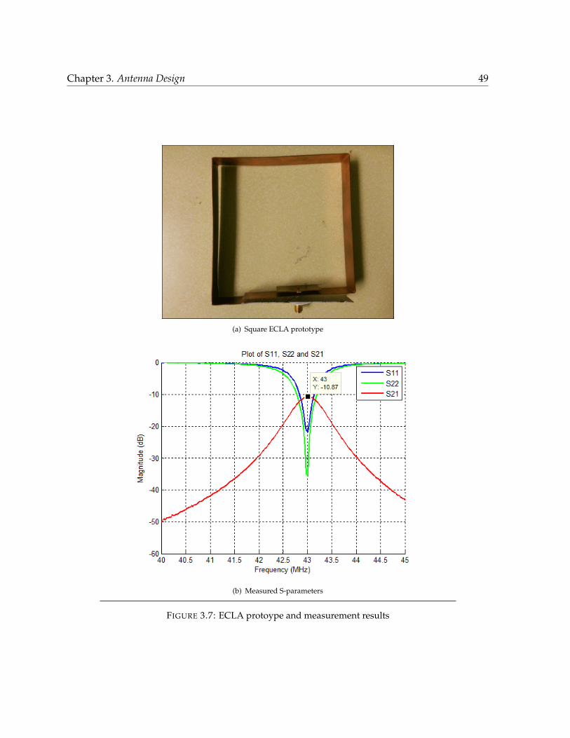
Chapter 3. Antenna Design 49
(a) Square ECLA prototype
(b) Measured S-parameters
FIGURE 3.7: ECLA protoype and measurement results
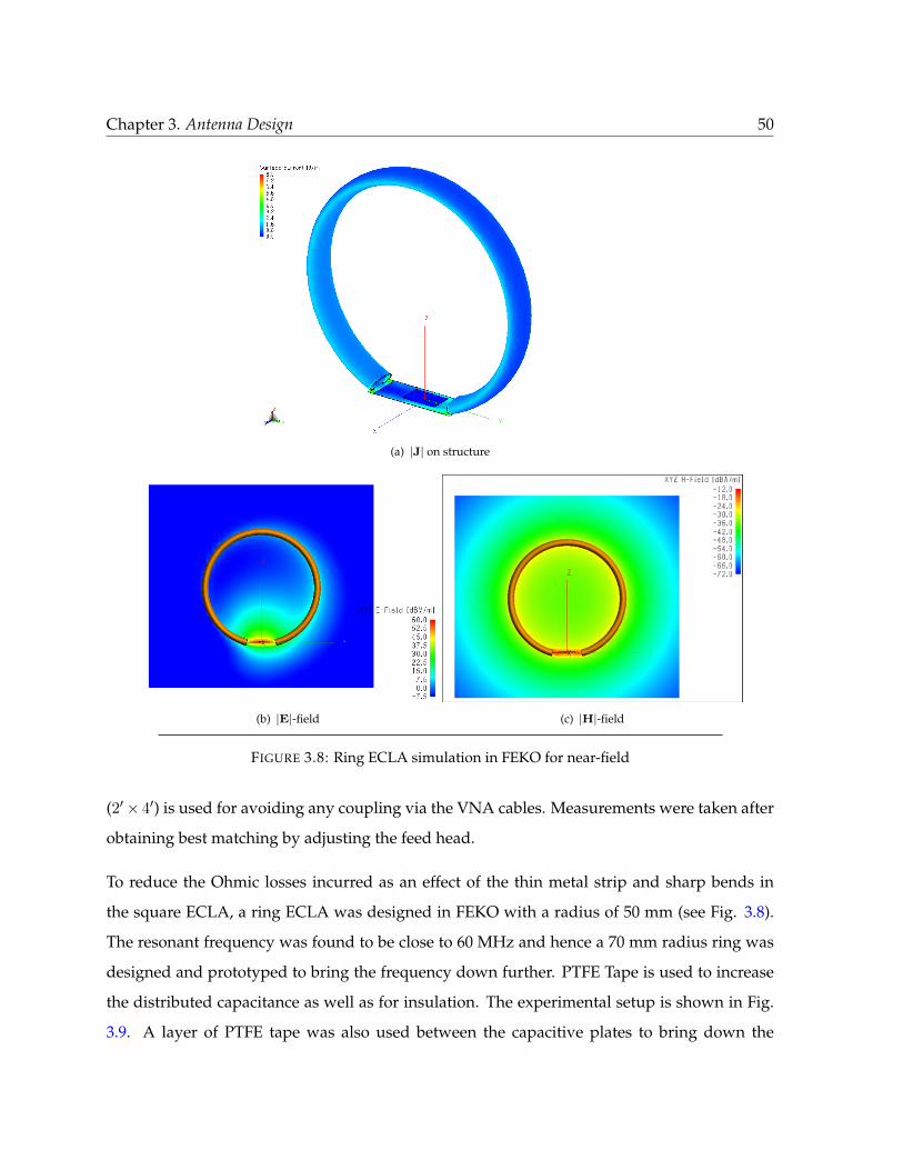
Chapter 3. Antenna Design 50
(a) |J| on structure
(b) |E|-field (c) |H|-field
FIGURE 3.8: Ring ECLA simulation in FEKO for near-field
(2′× 4′) is used for avoiding any coupling via the VNA cables. Measurements were taken after
obtaining best matching by adjusting the feed head.
To reduce the Ohmic losses incurred as an effect of the thin metal strip and sharp bends in
the square ECLA, a ring ECLA was designed in FEKO with a radius of 50 mm (see Fig. 3.8).
The resonant frequency was found to be close to 60 MHz and hence a 70 mm radius ring was
designed and prototyped to bring the frequency down further. PTFE Tape is used to increase
the distributed capacitance as well as for insulation. The experimental setup is shown in Fig.
3.9. A layer of PTFE tape was also used between the capacitive plates to bring down the
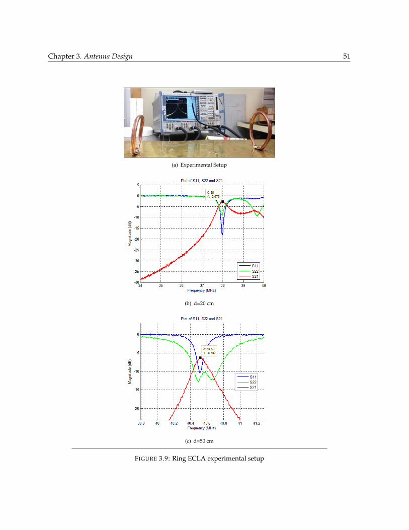
Chapter 3. Antenna Design 51
(a) Experimental Setup
(b) d=20 cm
(c) d=50 cm
FIGURE 3.9: Ring ECLA experimental setup
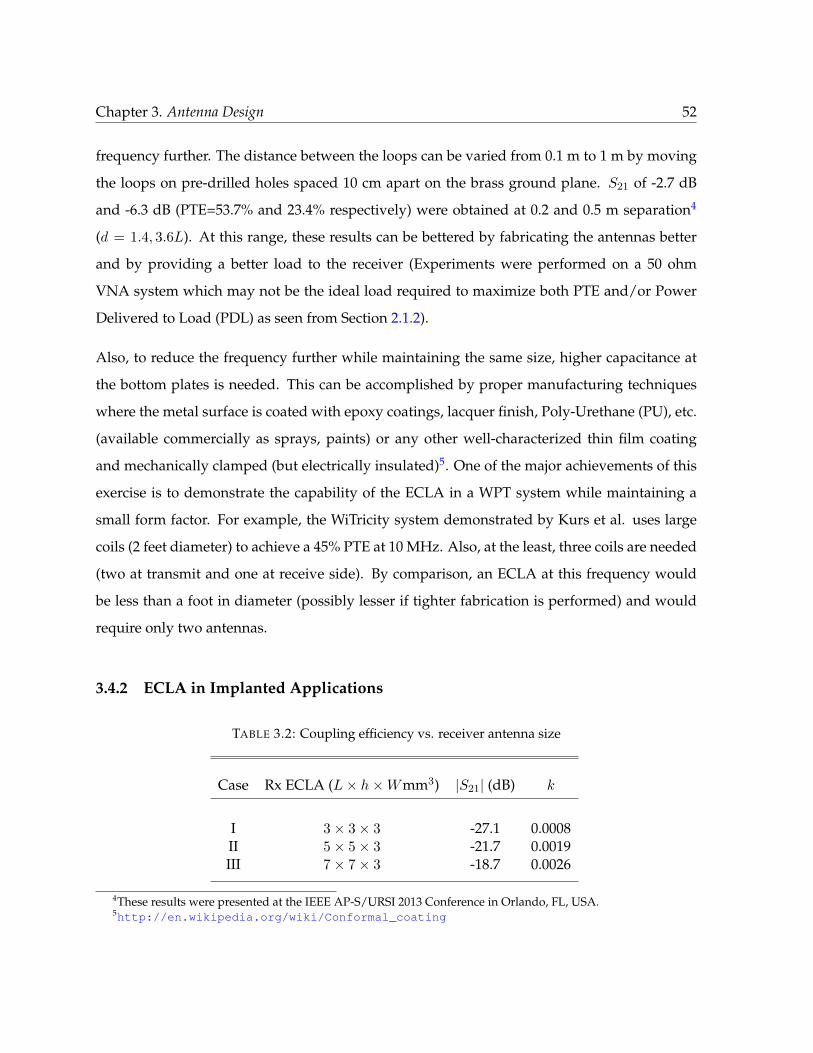
Chapter 3. Antenna Design 52
frequency further. The distance between the loops can be varied from 0.1 m to 1 m by moving
the loops on pre-drilled holes spaced 10 cm apart on the brass ground plane. S21 of -2.7 dB
and -6.3 dB (PTE=53.7% and 23.4% respectively) were obtained at 0.2 and 0.5 m separation4
(d = 1.4, 3.6L). At this range, these results can be bettered by fabricating the antennas better
and by providing a better load to the receiver (Experiments were performed on a 50 ohm
VNA system which may not be the ideal load required to maximize both PTE and/or Power
Delivered to Load (PDL) as seen from Section 2.1.2).
Also, to reduce the frequency further while maintaining the same size, higher capacitance at
the bottom plates is needed. This can be accomplished by proper manufacturing techniques
where the metal surface is coated with epoxy coatings, lacquer finish, Poly-Urethane (PU), etc.
(available commercially as sprays, paints) or any other well-characterized thin film coating
and mechanically clamped (but electrically insulated)5. One of the major achievements of this
exercise is to demonstrate the capability of the ECLA in a WPT system while maintaining a
small form factor. For example, the WiTricity system demonstrated by Kurs et al. uses large
coils (2 feet diameter) to achieve a 45% PTE at 10 MHz. Also, at the least, three coils are needed
(two at transmit and one at receive side). By comparison, an ECLA at this frequency would
be less than a foot in diameter (possibly lesser if tighter fabrication is performed) and would
require only two antennas.
3.4.2 ECLA in Implanted Applications
TABLE 3.2: Coupling efficiency vs. receiver antenna size
Case Rx ECLA (L× h×Wmm3) |S21| (dB) k
I 3× 3× 3 -27.1 0.0008II 5× 5× 3 -21.7 0.0019III 7× 7× 3 -18.7 0.0026
4These results were presented at the IEEE AP-S/URSI 2013 Conference in Orlando, FL, USA.5http://en.wikipedia.org/wiki/Conformal_coating
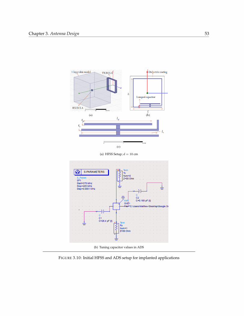
Chapter 3. Antenna Design 53
(a) HFSS Setup; d = 10 cm
(b) Tuning capacitor values in ADS
FIGURE 3.10: Initial HFSS and ADS setup for implanted applications
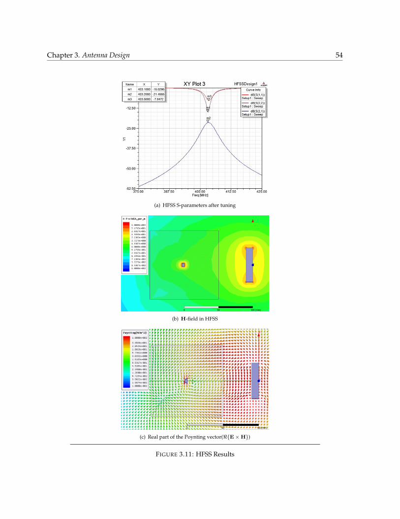
Chapter 3. Antenna Design 54
(a) HFSS S-parameters after tuning
(b) H-field in HFSS
(c) Real part of the Poynting vector(<E×H)
FIGURE 3.11: HFSS Results

Chapter 3. Antenna Design 55
One of the main issues with any implanted device is providing power to it. Those devices
which spend a short time in the human body can be easily fed by batteries. However, the
long-lived devices always need to be recharged or fed through a reliable energy harvesting
mechanism. This can be quite cumbersome especially when the implants are within the body
or trans/sub-cutaneous6. Existing techniques mostly use inductive loops that require one or
more conditioning (or repeater) stages coupled with matching networks at source and load
ends which tend to load them and reduce overall system efficiency due to losses incurred in
matching networks and parasitic coils [Guoxing et al., 2005, Kumar et al., 2009, Neihart and
Harrison, 2005, Ping et al., 2008, RamRakhyani et al., 2011, Si et al., 2007, Xiaoyu et al., 2009].
The ECLA, on the other hand, uses a capacitive feed which can be designed in order to do
away with any sort of matching network i.e. it can be directly fed and perfectly matched to a
transmission line or directly to a source/load.
The transfer of power to a device inside the human body is a complicated problem and arriving
at a reasonable model for such a link is a bit involved [Fotopoulou and Flynn, 2006, Guoxing
et al., 2005]. This is mainly due to the non-homogeneous and frequency-dependent dielectric
environment that the different parts of the human body offers to RF waves. Another constraint
in the case of implanted devices is the small form factor that is required to facilitate their use
inside the human body. We will mainly focus on the latter aspect in this section. Therefore,
in order to better understand the effect of the variation in size of the receiving antenna on
the PTE, we will also study the case where two ECLAs are used as transmitter and receiver.
In this section, we modify the ECLA design for implanted applications by miniaturizing it
considerably. This can be achieved in two ways:
• In a traditional sense, surrounding the antenna in a dielectric material with a bio-compatible
insulation layer to increase the electrical length (d/λ) of the antenna.
• Since the ECLA uses distributed capacitors for feeding as well as for achieving self-
resonance (see Table. 3.1), a high-Q lumped capacitor can be added in parallel to the
6http://www.embedded.com/design/connectivity/4025029/The-challenge-of-designing-in-body-communications

Chapter 3. Antenna Design 56
frequency-controlling tp height to increase the capacitance and lower the frequency of
operation to a desirable frequency.
Choice of Full-wave Solver: Note that in typical implanted applications, such as for a pace-
maker or a sensor inside the body, the implanted antenna (receiver) is heavily miniaturized but
the source or transmit antenna outside the body does not necessarily have to be small. Biomed-
ical applications such as these are inherently a material half-space problem [King et al., 1981,
Smith, 1984] and care must be taken in defining the near-zone as power transfer may occur due
to hybrid modes at mid to high distances. For studying this half-space problem, HFSS is used
over FEKO, due to the latter’s difficulty in dealing with dielectric boundaries (MoM engines
typically behave irregularly with dielectric interfaces; however, to be fair, FEKO does have an
FEM engine and a hybrid solver that the author hasn’t tried yet.).
The PTE can be considered to be the value of |S21|2 as it encapsulates the coupling effects
between the two antennas and gives an idea of available power [Gonzalez, 1984] transferred
from one port to the other[Nambiar and Manteghi, 2014b]. Full-wave EM simulations are
carried out in HFSS to obtain PTE followed by a circuit-level analysis using ADS to obtain a
value for coupling coefficient, k. Ascertaining k is important as it can facilitate a better design
procedure for the antennas and gives a better understanding of the coupling and the overall Q
of the system.
The HFSS simulation setup for 403 MHz MICS band WPT for implanted applications is shown
in Fig. 3.10. After an initial run, the S-parameter file from HFSS in input to an ADS schematic
where the extra capacitor ports are varied in capacitance to achieve operation at the correct
frequency. These values are then fed back to the HFSS model and simulated as a final test.
An associated problem that arises here is that the initial HFSS simulation contains a solution
for a frequency set by the user that very well isn’t resonant, at least not at the final desired
frequency. However, results were not far from that expected and a small amount of tuning is
usually enough to set the antennas to the desired frequency of operation. This hybrid approach
of using both HFSS and ADS results in considerable savings in time and computational effort.

Chapter 3. Antenna Design 57
The setup consists of two ECLAs, one as a transmitter located in free space and another coated
by a polystyrene film (for biocompatibility) of dielectric constant, εr = 2.07, and embedded
within a block of dry skin with equivalent εr = 49.7 [Gabriel et al., 1996]7. A lumped capacitor is
used to miniaturize the implanted antenna. An equivalent single layer of skin tissue is chosen
to keep the simulation simple. The transmitter dimensions are 50 × 50 × 10mm3 (L × h ×W )
and the dimensions of the implanted antenna are varied as shown in Table. 3.2 separated by
d = 100 cm. The ADS equivalent circuits discussed in 3.3 were then matched in terms of
component values to fit the full-wave simulation results such that a representative value of k
may be obtained. From Chapter 2, we know that
PTE = k2Q1Q2 (3.1)
whereQ1, Q2 are the loaded quality factors of the antennas. Thus, by modeling the link in ADS,
we can get a better understanding of the design aspects of the system as well. The results for
the final design for Case II of Table. 3.2 are shown in Fig. 3.11 [Nambiar and Manteghi, 2014a].
As expected, a smaller-sized implanted antenna gives a lower value of PTE. However, it is
interesting to note that the coupling regime is of a very loosely-coupled system as seen by the
magnitude of k (< 0.01). From this we can see that the full wave results and the ADS modeling
technique can be compared for a given load impedance and to characterize the power transfer
channel purely through the coupling factor, k.
Some prototyped antennas (courtesy of Dr. Manteghi) are shown in Fig. 3.12. These antennas
are found to resonate at 449.5 MHz (as some capacitor values needed for MICS band operation
were not readily available) and measurement results are seen in Fig. 3.13. As was the case
before, a brass sheet acts as a ground plane and the Tx ECLA is modified for 450 MHz operation
(30 × 30 × 10mm3). Miniaturization of the antenna was made possible by adding a high-Q
lumped capacitor to the distributed capacitor. An |S21| of -35 dB was obtained at a distance
of 10 cm in free space which is far below our expectations. However, these results may be
7http://transition.fcc.gov/oet/rfsafety/dielectric.html
Chapter 3. Antenna Design 58
(a) 5× 5× 3mm3 with lumped capacitor
(b) (c) Other prototype variations
FIGURE 3.12: Miniaturized ECLA prototypes using additional lumped capacitor where neces-sary
justified by the limited manufacturing capabilities available at the time and poor RL of the
small antennas.
Even though the HFSS results were encouraging, they fail to give a complete picture as regards
the actual performance of the system when used inside the human body. Remcom’s XFDTD 7
(XF7) is a Finite Difference Time Domain (FDTD) solver that has a human body voxel model
with mm-level resolution8. Fig. 3.14 shows the setup in XF7 and the resulting |S21| at d = 40, 65
8CST also has a human body solver but Remcom graciously allowed the use of their models for free. FEKO alsosupports human tissue models and SAR calculation but was not used due to lack of a human model.
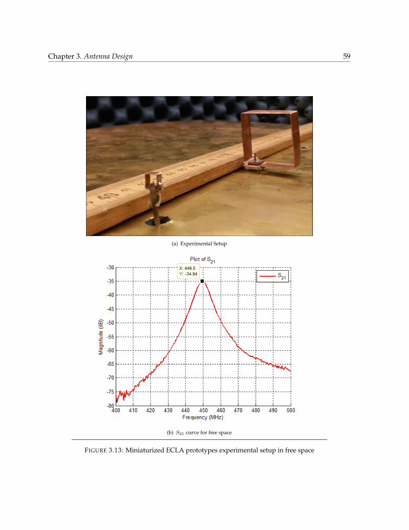
Chapter 3. Antenna Design 59
(a) Experimental Setup
(b) S21 curve for free space
FIGURE 3.13: Miniaturized ECLA prototypes experimental setup in free space
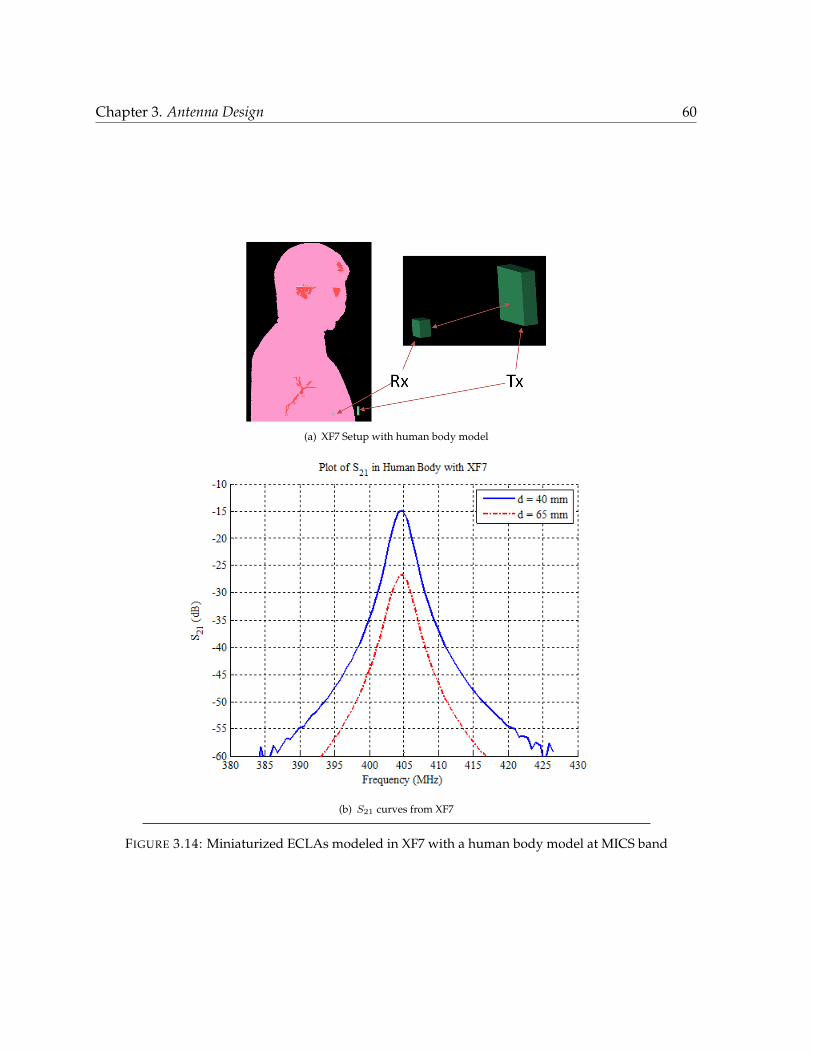
Chapter 3. Antenna Design 60
(a) XF7 Setup with human body model
(b) S21 curves from XF7
FIGURE 3.14: Miniaturized ECLAs modeled in XF7 with a human body model at MICS band
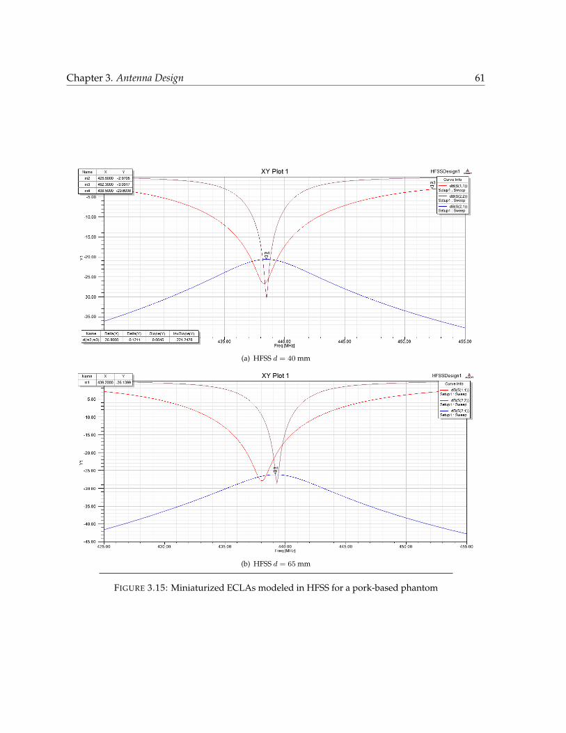
Chapter 3. Antenna Design 61
(a) HFSS d = 40 mm
(b) HFSS d = 65 mm
FIGURE 3.15: Miniaturized ECLAs modeled in HFSS for a pork-based phantom

Chapter 3. Antenna Design 62
mm for an implanted antenna in the chest region. The results are very encouraging mainly due
to the fact that the implanted antenna sits in front of the lungs that are primarily air-filled.
In order to actually be able to test the setup in an environment that emulates the human body,
a tub of ground pork meat can be used. In order to calculate the electrical properties of the
meat, the weighted average of human protein and fat values in the ratio 2:1 (assuming that
pork muscle and fat values share the same electrical nature as corresponding human tissues) is
taken for finding the required dielectric constant and conductivity. These values are obtained
for a frequency of 403 MHz and summarized in Table. 2.1.
εr =11.6 + 2× 58.8
3= 43.067
σ =0.08 + 2× 0.84
3= 0.587 S/m
ρ =920 + 2× 1040
3= 1000 kg/m3
With these values, a one-layer equivalent model was created in HFSS with dimensions of 90×
90× 180mm3 with the Tx facing the 180× 90mm2 face of the pork model in a setup similar to
that shown in Fig. 3.10. The resulting curves are shown in Fig. 3.15.
The experimental setup corresponding to the HFSS experiment and the resulting measured
S-parameters are shown in Fig. 3.16 for two distances of 40 mm and 65 mm, respectively. As
shown, an |S21| of -25dB was obtained at a distance of 40mm through the pork phantom9.
Some further modifications to the implanted design may be made as shown in Fig. 3.17 to
reduce the SAR. For further reading on the performance of the ECLA in the human body,
please refer to Ibraheem and Manteghi [2014a,b].
9These results were presented at the IEEE AP-S/URSI 2014 Conference in Memphis, TN, USA.
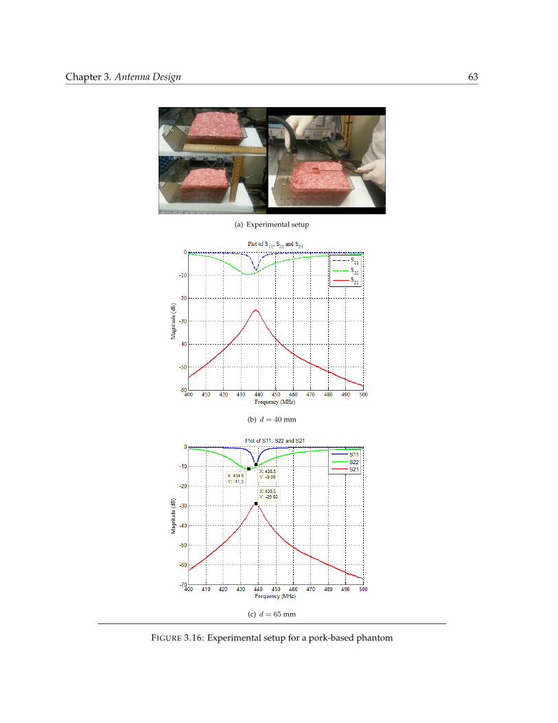
Chapter 3. Antenna Design 63
(a) Experimental setup
(b) d = 40 mm
(c) d = 65 mm
FIGURE 3.16: Experimental setup for a pork-based phantom

Chapter 3. Antenna Design 64
(a) Modified dielectric coating (b) SAR for an implanted ECLA in the head
FIGURE 3.17: Medical applications

Chapter 4
System Design
4.1 Overview
In this chapter, we will focus on the design of the oscillator and load to complete the Wireless
Power Transfer (WPT) system. Specifically, some design methods for a negative resistance os-
cillator will be presented and the ways by which a load can be analyzed at the source side are
discussed. The objective here is to maximize the Power Delivered to Load (PDL) by choos-
ing the right system goals and obtaining the highest efficiency throughout the system - from
source to load. For example, as seen from the last chapter, for most implanted applications that
function off of a coin cell (CR2032 Li/MnO type), the maximum power deliverable is of the or-
der of 0.5 W. With an S21 of -20 dB, this implies 500 mW of continuous power to an implanted
device at a depth of 5 cm would require a 50 W transmitter outside the human body. For most
applications, this is a rather high value but the idea is that such a system would have to be able
to compensate for the path loss (1-PTE) by delivering suitable power at the transmit antenna
port. Typically, 100 mW of power is a sufficient figure [Catrysse et al., 2004, Ghovanloo and
Najafi, 2007, Wang et al., 2006] to deliver to an implanted device.
In the literature, considerable effort has gone into designing systems with high Power Transfer
Efficiency (PTE) and high PDL (as seen in Chapter 2); however, an effort to study the effect of
65

Chapter 4. System Design 66
the loaded WPT system on a stand-alone source has not been studied to the best of the author’s
knowledge. Some patent arts establish the use of negative resistance generators but no analysis
is presented on how to design these oscillators keeping in mind the figures of merit of a WPT
system [Mohammadian, 2009, Toncich et al., 2009]. In this chapter, a negative resistance based
oscillator design is proposed for a WPT transmitter. The need for such an oscillator stems from
the fact that the antenna is a one-port device and in such cases it is difficult to efficiently in-
corporate it into the feedback loop of a conventional high-power and high-efficiency oscillator
design. Although ultra high efficiency oscillators are not discussed here (such as Class E and
above), some design methodologies are discussed from the specific viewpoint of a WPT system
and presented in this chapter. Both the free-space and implanted cases discussed in Chapter 3
are considered here and design presented. However, only the free-space case is fabricated.
Although this chapter primarily discusses oscillator design, it is titled System Design as we
now integrate the previously discussed WPT terms into the oscillator design process, thus
completing a closed system where the parameters are interlinked to each other.
4.2 Oscillator Design
As discussed above, the reason that we need a negative resistance oscillator is due to the fact
that we are feeding an unbalanced antenna like the Electrically Coupled Loop Antenna (ECLA)
. Unlike inductive loops that are common in WPT literature which can be fed by incorporating
them into the feedback network of classical oscillator designs like a Colpitts oscillator, a nega-
tive resistance oscillator has its own set of design challenges but like any other oscillator also
follows the same basic principles. In a feedback oscillator, the feedback path and the associated
gain and phase values can be computed quite easily. Doing so may not be inherently apparent
but the right analysis shows the similarities in design as well as brings out the load or match-
ing network requirements. There are a few design approaches that can be taken that lead to
some very useful insights and in this section we will try to cover a couple of them from a WPT
perspective. A thorough and rigorous non-linear analysis can often lead to a very accurate
prediction of the final amplitude and frequency level of the oscillation signal. The goal here

Chapter 4. System Design 67
is to design an oscillator that operates at the final operational power level of the source ECLA
with high efficiency while keeping components at a minimum to keep system complexity low.
4.2.1 Negative Resistance Oscillators
At first glance, a negative resistance may seem non-physical but it can be understood intu-
itively as an active-device based phenomenon (since passives can only lead to loss/positive
resistance). Thus, from an RF perspective, we see that these are the loads that lie outside of
the Smith chart. In order to achieve negative resistance, the most important requirement is
that of the design of a proper termination network for a given load impedance such that the
magnitude of the reflection coefficient, |Γin|, is larger than 1 (outside the Smith Chart). Gonza-
lez [1984], Grebennikov [2007] present some good analytical and empirical techniques for the
establishment of oscillations, their stability, phase noise characteristics and other important
parameters.
Generally, for high power applications as well as for two-port analysis, a tuned base (inductor
to base) is employed as the reflection coefficients are then seen to trace constant susceptance
curves with increasing signal level [Rhea, 1995]. These are then negative conductance devices
as they require a parallel resonator structure. The ECLA can be seen from its equivalent circuit
to resemble a parallel resonator. A tuned base transistor can also be thought of as a Clapp os-
cillator. In order to better understand the working of oscillators, we establish the mathematical
formulation in the next section.
4.2.2 Mathematical Description
We begin by considering Fig. 4.1 where a conventional feedback network system is shown
[Gonzalez, 1984]. We can define some of the quantities shown as
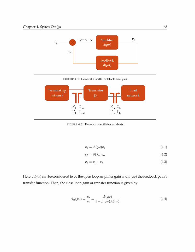
Chapter 4. System Design 68
FIGURE 4.1: General Oscillator block analysis
FIGURE 4.2: Two-port oscillator analysis
vo = A(jω)vd (4.1)
vf = β(jω)vo (4.2)
vd = vi + vf (4.3)
Here,A(jω) can be considered to be the open loop amplifier gain and β(jω) the feedback path’s
transfer function. Then, the close-loop gain or transfer function is given by
Acl(jω) =vovi
=A(jω)
1− β(jω)A(jω)(4.4)

Chapter 4. System Design 69
Then the Barkhausen criteria is achieved for vi = 0 (or by finding the poles of Equation 4.4),
i.e.
β(jω)A(jω) = 1 (4.5a)
where β(jω) = βr(ω) + jβi(ω) (4.5b)
A(jω) =1
βr(ω)(4.5c)
βi(ω) = 0 (4.5d)
These equations establish the gain and frequency of the oscillations. It can also be seen that the
oscillation condition survives as long as
RIN (Ao, ωo) +RL(ωo) = 0 (4.6)
and
XIN (Ao, ωo) +XL(ωo) = 0 (4.7)
which translates to the point that the oscillations exist as long as the load resistance is less
than the magnitude of the negative resistance while maintaining phase conditions. Also, from
Kurokawa [1969], we find that the stability of the oscillations can be predicted by
∂RIN (A)
∂A|A=Ao
dXL(ω)
dω|ω=ωo −
∂XIN (A)
∂A|A=Ao
dRL(ω)
dω|ω=ωo > 0 (4.8)
In most cases, dRL(ω)dω = 0, but this is only true for a truly static load. In the case of WPT, this
would mean a fixed load at a fixed distance having some known coupling factor. In the case
where dRL(ω)dω = 0, we can arrive at the relation
RL =R0
3(4.9)

Chapter 4. System Design 70
to maximize the oscillation power, where R0 is the termination network resistance (if Termina-
tion Network impedance is given by ZT = R0 + jX0)[Gonzalez, 1984]. This provides a good
starting point for the oscillator design problem.
Consider Fig. 4.2 where a two-port system is shown with one port labeled the termination
port while the other is the load port where the termination and load networks are connected
respectively. Also, after some manipulation, we can arrive at the two-port RF equivalent of the
oscillation conditions [Gonzalez, 1984], giving
ΓINΓL = 1 (4.10)
ΓL =1
ΓIN=
1− S22ΓTS11 −∆ΓT
(4.11)
or ΓT =1− S1ΓLS22 −∆ΓL
(4.12)
ΓOUT =S22 −∆ΓL1− S11ΓL
(4.13)
ΓOUTΓT = 1 (4.14)
General Design Procedure [Gonzalez, 1984]
1. Use a potentially unstable transistor at the design frequency
2. Design a terminating network to make |ΓIN | > 1 using series or shunt feedback.
3. Design a load network to resonate ZIN such that
XL(ω0) = −XIN (ω0) (4.15)
and
RL =R0
3(4.16)

Chapter 4. System Design 71
It can also be seen that both load and termination networks oscillate at resonance and that the
actual frequency of oscillation is controlled by when the positive and negative resistances can-
cel each other out in the network. Hence, some degree of tuning will be required. Also note
that since S-parameters are by their very nature small-signal and linear measurements/char-
acteristics of the device, some variation from the predictions should be expected as oscillators
are non-linear systems (by the virtue of their large-signal behavior).
An alternative design approach based on material given in Rhea [1995] will be presented along
with the simulation results in following sections.
Transformation
Notice that the equations presented above give the design values in case of a constant load.
Since we know that in the case of WPT, our load (as seen from the source) is not constant,
some amount of flexibility is required in the termination network which is one of the more
important problems associated with this method. However, if a convenient “calibration” curve
or variation in load with distance information is at our disposal, then this information can be
used to design a smarter source termination network. This is where the techniques presented in
the previous chapters such as extraction of k from the equivalent circuit come into play. Thus,
this information is embedded into the coupled antenna’s reflection coefficient and can be used
to incorporate coupling characteristics into the oscillator design. Also, since the oscillation
conditions rely heavily upon the load impedance, we can achieve some amount of frequency
tracking by virtue of the negative resistance design.
4.3 Simulation Results
In this section, we will aim to design and simulate a few circuits using the approach presented
earlier while trying to maximize the efficiency and power delivered by the oscillator. It is, how-
ever, beneficial to study the Bode plots of the open loop (or two-port) network as an amplifier

Chapter 4. System Design 72
to gain more insight into the problem1
Choice of Transistor
Although the circuits given in Rhea [1995] form the basis of the schematics given in the subse-
quent sections and which use the MRF559 transistor, we will use the MRF555 where possible as
this is but a higher power version of the MRF559 (Ic = 500 mA vs Ic = 150 mA). Both are now
mostly obsolete but the abundance of design schematics in the literature for these devices and
their trusted RF performance makes them a good candidate for our application. The transistors
used in the prototype were ordered from RFparts.com.
PBJT vs. S-Parameter models
ADS offers two models for us to work with, namely, a packaged BJT model containing all the
known packaged parasitics, and an S-parameter model for a given set of bias conditions. Note
that the former is a large-signal model and thus can be used for oscillator analysis while the
latter is suitable for amplifier design and to study the response of the transistor in its linear
region. A transient or harmonic balance analysis of the oscillator is not possible with the S-
parameter model.
Note that to obtain the PBJT and S-parameter models, it is first necessary to unzip the de-
sign kits (RF Transistor Library) located in the “oalib” folder of the ADS installation directory.
Analog Parts library contains the non-linear SPICE models of transistors for use at frequencies
less than 10 MHz. Even though not suited for our purposes, it is compared to the PBJT and
S-parameter models as an educational exercise below.
Fig. 4.3 shows the circuit setup to compare the various MRF559 models for a tuned base case
with circuit DC conditions matching that of the S-parameter data. Fig. 4.4 shows the [S] matrix
values for the models for frequencies from 300 MHz to 1 GHz. Clearly, the S-parameter data
is not at all very well-aligned with the PBJT results. This could be due to the difference in bias
conditions that existed for the S-parameter data setup (which we have no access to sadly) that
might change the feedback mechanisms in play for the S-parameter model vs the PBJT model.
1An old adage goes: to realize an amplifier, design an oscillator; to realize an oscillator, design an amplifier!
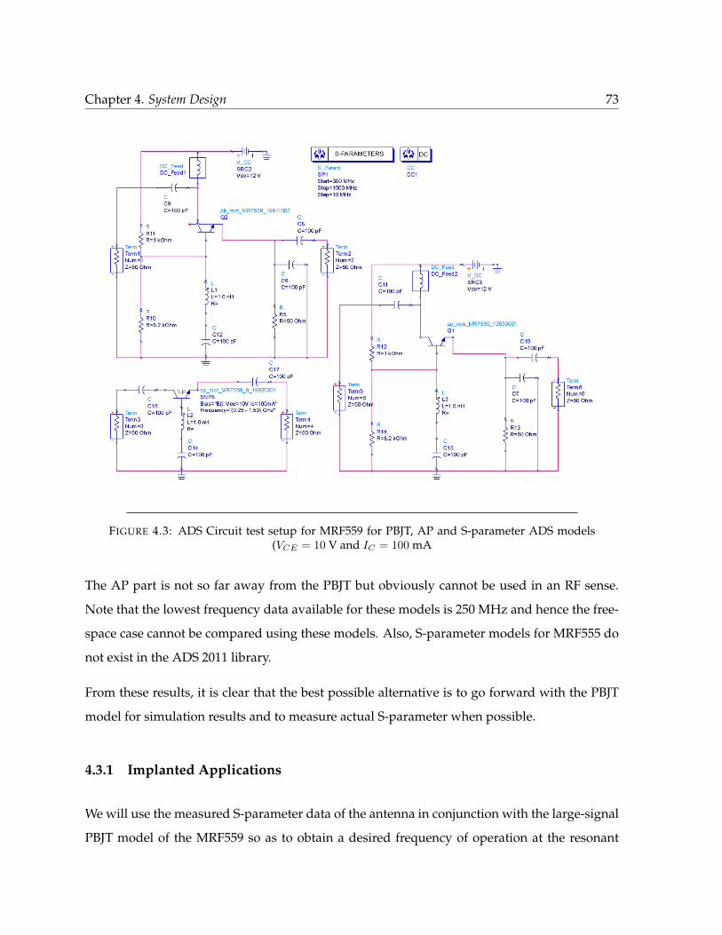
Chapter 4. System Design 73
FIGURE 4.3: ADS Circuit test setup for MRF559 for PBJT, AP and S-parameter ADS models(VCE = 10 V and IC = 100 mA
The AP part is not so far away from the PBJT but obviously cannot be used in an RF sense.
Note that the lowest frequency data available for these models is 250 MHz and hence the free-
space case cannot be compared using these models. Also, S-parameter models for MRF555 do
not exist in the ADS 2011 library.
From these results, it is clear that the best possible alternative is to go forward with the PBJT
model for simulation results and to measure actual S-parameter when possible.
4.3.1 Implanted Applications
We will use the measured S-parameter data of the antenna in conjunction with the large-signal
PBJT model of the MRF559 so as to obtain a desired frequency of operation at the resonant
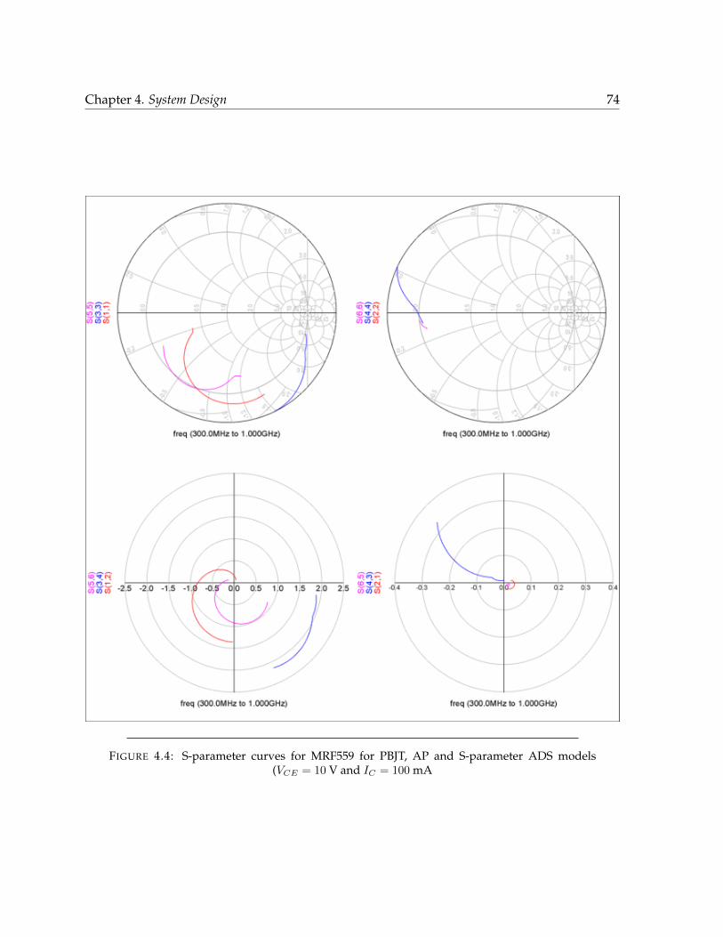
Chapter 4. System Design 74
FIGURE 4.4: S-parameter curves for MRF559 for PBJT, AP and S-parameter ADS models(VCE = 10 V and IC = 100 mA

Chapter 4. System Design 75
frequency of the antenna. At first, it may seem counter-intuitive to design an oscillator based
on the measured linear S-parameter data but it is important to realize that the antenna itself
is an LTI (Linear Time Invariant) system and the mostly non-linear component is that of the
transistor which is modeled effectively by the ADS PBJT model.
Two-port analysis
The results presented here are the result of several iterations of design and simulation and only
the final result is shown here in the interest of brevity and conciseness.
From Fig. 4.5, S-parameter data from Coilcraft is used to model the effect of “real” inductors
on the circuits. The circuit is tuned so as to achieve maximum values of S11, S22 while also
achieving a phase reversal in the gain term (S12). Fig. 4.6 shows the stability analysis of the
system which shows the network is clearly unstable as K < 1 and |∆| > 1. From Fig. 4.7,
a lower frequency is chosen for the two-port analysis and design as it was found (through
various iterations) that the oscillator had a tendency to oscillate at roughly a 20-40 MHz higher
frequency with tuning.
For the design of a terminating network for the measured antenna load, a MATLAB code is
used to calculate the network values (see Appendix B).
Transient analysis
Fig. 4.8 shows the transient analysis setup in ADS. The measured antenna parameters (charac-
terized from 300 - 500 MHz) are connected at the node marked ‘Vterm’ (Both Termination and
Load ports oscillate and therefore can be used interchangeably. Also, there are some efficiency
benefits to having a lower resistance value in the passive fixed network). The time response of
the circuit is shown in Fig. 4.9 showing the buildup of oscillation in the network at the antenna
port. The FFT of the (truncated) time response is given in Fig. 4.10 and shows that the max-
imum power is a slightly higher frequency of 480 MHz, which can be tuned down by proper
tuning techniques (discussed in 4.3.4). Also note the excellent 2nd harmonic suppression (> 20
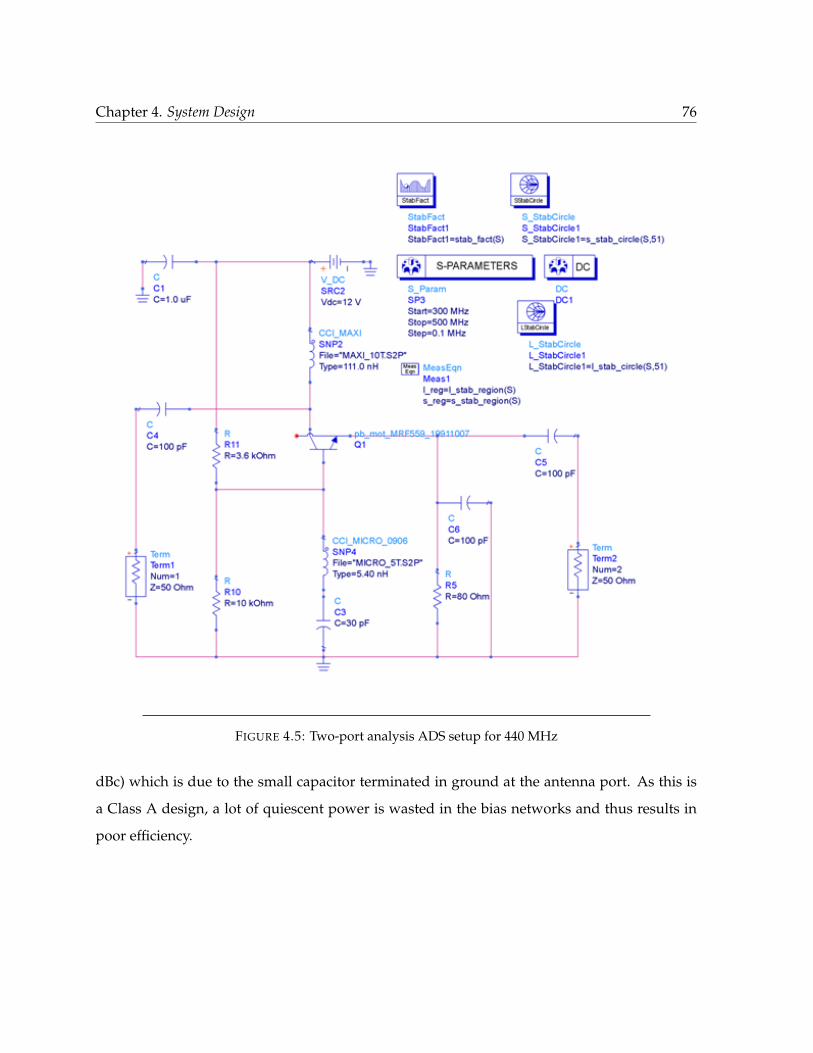
Chapter 4. System Design 76
FIGURE 4.5: Two-port analysis ADS setup for 440 MHz
dBc) which is due to the small capacitor terminated in ground at the antenna port. As this is
a Class A design, a lot of quiescent power is wasted in the bias networks and thus results in
poor efficiency.
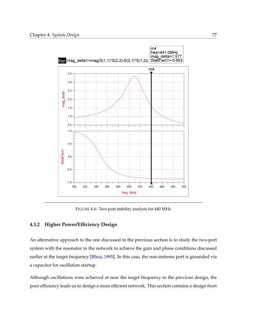
Chapter 4. System Design 77
FIGURE 4.6: Two-port stability analysis for 440 MHz
4.3.2 Higher Power/Efficiency Design
An alternative approach to the one discussed in the previous section is to study the two-port
system with the resonator in the network to achieve the gain and phase conditions discussed
earlier at the target frequency [Rhea, 1995]. In this case, the non-antenna port is grounded via
a capacitor for oscillation startup.
Although oscillations were achieved at near the target frequency in the previous design, the
poor efficiency leads us to design a more efficient network. This section contains a design from

Chapter 4. System Design 78
FIGURE 4.7: Two-port analysis S-parameter data for 440 MHz

Chapter 4. System Design 79
FIGURE 4.8: Transient analysis ADS setup for 440 MHz
Rhea [1995] that proposes a hybrid Class A and C type operation resulting in higher operating
efficiency and thus, power.
The proposed design is shown in Fig. 4.11 with the results in Fig. 4.12 and Fig. 4.13. The
resulting frequency is higher than expected but we can see that the efficiency is pretty high
thus validating the use of this approach. Some tuning may be required post-fabrication to
achieve the correct oscillation frequency. Also note that the peak current does not exceed the
device rating of 500 mA.
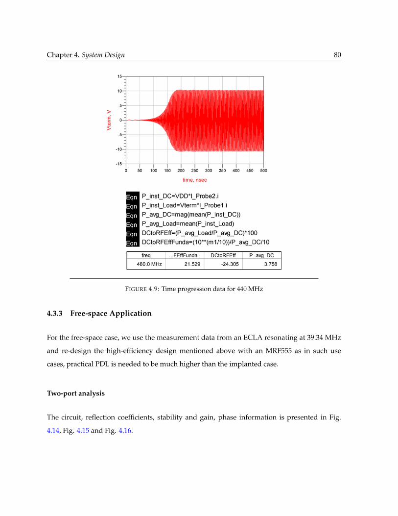
Chapter 4. System Design 80
FIGURE 4.9: Time progression data for 440 MHz
4.3.3 Free-space Application
For the free-space case, we use the measurement data from an ECLA resonating at 39.34 MHz
and re-design the high-efficiency design mentioned above with an MRF555 as in such use
cases, practical PDL is needed to be much higher than the implanted case.
Two-port analysis
The circuit, reflection coefficients, stability and gain, phase information is presented in Fig.
4.14, Fig. 4.15 and Fig. 4.16.
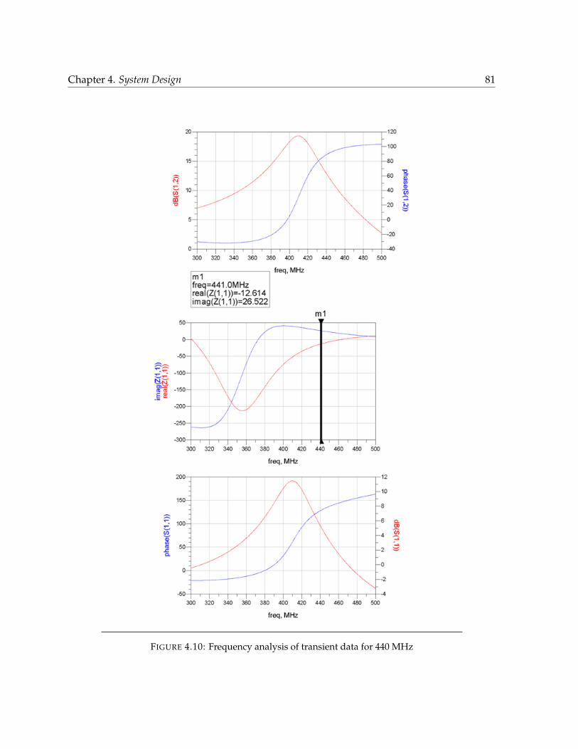
Chapter 4. System Design 81
FIGURE 4.10: Frequency analysis of transient data for 440 MHz
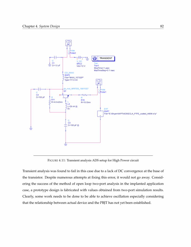
Chapter 4. System Design 82
FIGURE 4.11: Transient analysis ADS setup for High Power circuit
Transient analysis was found to fail in this case due to a lack of DC convergence at the base of
the transistor. Despite numerous attempts at fixing this error, it would not go away. Consid-
ering the success of the method of open loop two-port analysis in the implanted application
case, a prototype design is fabricated with values obtained from two-port simulation results.
Clearly, some work needs to be done to be able to achieve oscillation especially considering
that the relationship between actual device and the PBJT has not yet been established.
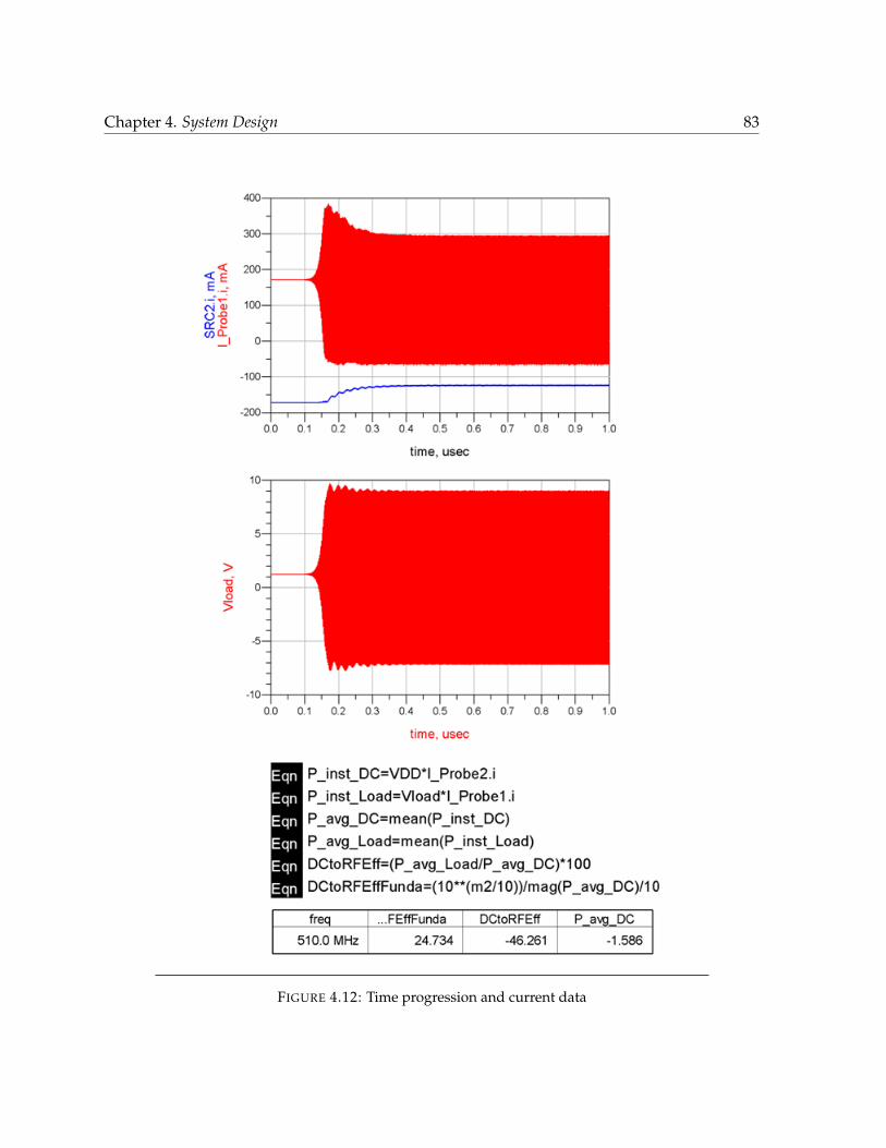
Chapter 4. System Design 83
FIGURE 4.12: Time progression and current data
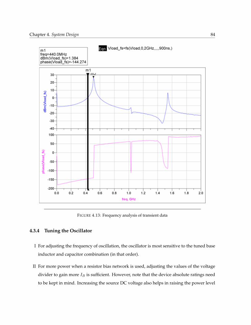
Chapter 4. System Design 84
FIGURE 4.13: Frequency analysis of transient data
4.3.4 Tuning the Oscillator
I For adjusting the frequency of oscillation, the oscillator is most sensitive to the tuned base
inductor and capacitor combination (in that order).
II For more power when a resistor bias network is used, adjusting the values of the voltage
divider to gain more IB is sufficient. However, note that the device absolute ratings need
to be kept in mind. Increasing the source DC voltage also helps in raising the power level
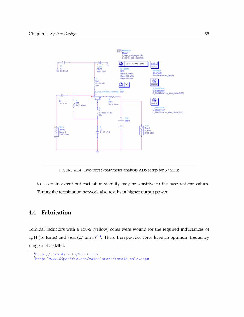
Chapter 4. System Design 85
FIGURE 4.14: Two-port S-parameter analysis ADS setup for 39 MHz
to a certain extent but oscillation stability may be sensitive to the base resistor values.
Tuning the termination network also results in higher output power.
4.4 Fabrication
Toroidal inductors with a T50-6 (yellow) cores were wound for the required inductances of
1µH (16 turns) and 3µH (27 turns)2 3. These Iron powder cores have an optimum frequency
range of 3-50 MHz.
2http://toroids.info/T50-6.php3http://www.66pacific.com/calculators/toroid_calc.aspx
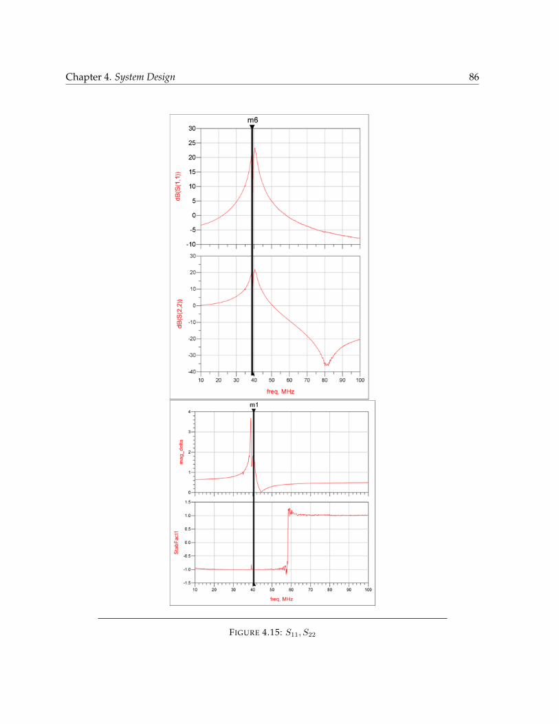
Chapter 4. System Design 86
FIGURE 4.15: S11, S22
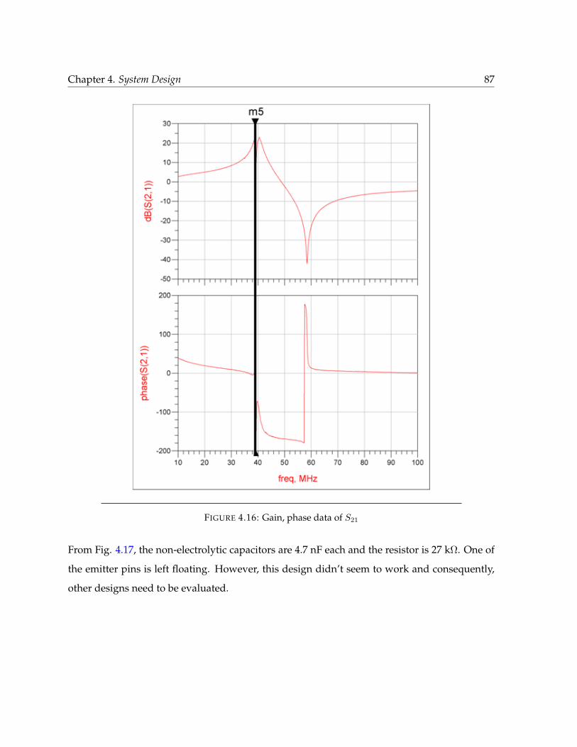
Chapter 4. System Design 87
FIGURE 4.16: Gain, phase data of S21
From Fig. 4.17, the non-electrolytic capacitors are 4.7 nF each and the resistor is 27 kΩ. One of
the emitter pins is left floating. However, this design didn’t seem to work and consequently,
other designs need to be evaluated.
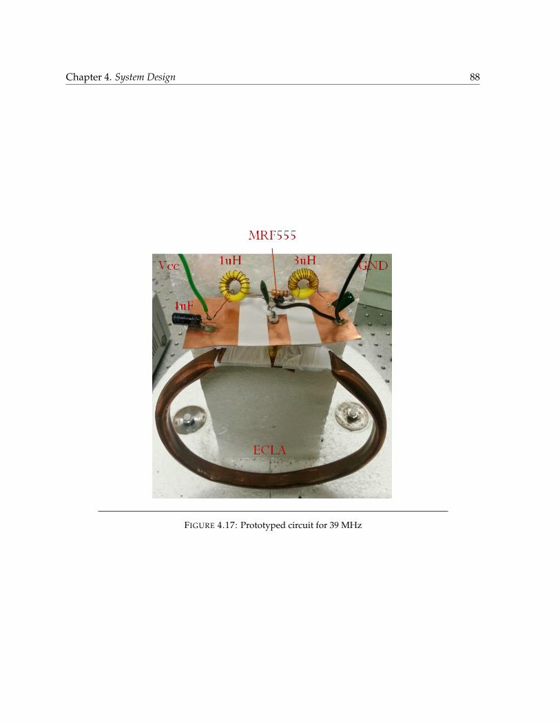
Chapter 4. System Design 88
FIGURE 4.17: Prototyped circuit for 39 MHz

Chapter 5
Conclusions and Future Work
5.1 Conclusions
In this thesis, various aspects of a Wireless Power Transfer (WPT) system design have been
considered, starting from the analysis of WPT systems using various theoretical techniques
for both free-space and implanted applications to the design of high-Q antennas for coupling
and finally the oscillator design to power such applications. It was shown that the Power
Transfer Efficiency (PTE) and Power Delivered to Load (PDL) of the system, though related to
each other, can both be independently maximized without simultaneously maximizing both
of them. Thus, for a practical system where PDL is most important, a system design perspec-
tive yields the tradeoffs between PTE and PDL even more clearly. The requirements for various
WPT couplers were studied and the Electrically Coupled Loop Antenna (ECLA) was proposed
as a suitable high-Q resonator for coupling. Miniaturization of the ECLA for implanted ap-
plications was studied and some design models proposed for various form factors. Further,
experimental results validated the use of ECLAs for implanted applications when manufac-
tured with suitable processes. A negative resistance oscillator was proposed to integrate the
coupling parameters into the system design. Various circuit topologies were studied for their
gain, efficiency and frequency dependence. Even though a successful prototype did not result
89

Chapter 5. Conclusions and Future Work 90
(mainly due to the high-Q nature of the ECLA), the design and prototyping efforts given here
should provide a platform from which a working prototype may be fabricated.
5.2 Future Work
This thesis gives but a preliminary analysis of the scope of system design tools to synthesize
a complete WPT system. Further work must be done to create a practical system. The author
believes that the following points give good direction to future research in this area.
• Antenna and EM analysis at coupling frequency(/ies) for tight and moderate coupling:
Preliminary results show some interesting results that need to be thoroughly studied.
Fig. 5.1 shows a 10 dB drop in far-field gain at the higher frequency that arises due to
frequency splitting of tight coupling. This means that most of the energy gets coupled to
the load at this frequency and thus, this frequency needs to be preferentially targeted for
operation at maximum PDL.
• Study the variation in Q and damping factor by having receiver circuitry that synchro-
nizes with the transmitter to give the best overall system performance. For example, a
circuit topology or receiver feedback system that involves manipulation of the load con-
ditions (say, a sweep of the resistance over a known value and period of time) that are
easily detectable to the oscillator as variation in load pull can be exploited to get a better
understanding of the k of the link(s) and modify the matching impedances on the fly and
perform optimally at any distance or operating point.
• Use an array of transmitter and receiver antennas to direct energy efficiently. Possibility
of exploiting supermodes by having side-by-side transmitters.
• Study the effect of having multiple receivers on overall coupling [Lee and Cho, 2015].
• Better, efficient circuitry is needed. It might be easier to use a Phased Locked Loop
(PLL) and a Power Amplifier to achieve better frequency stability, more power and circuit
flexibility.
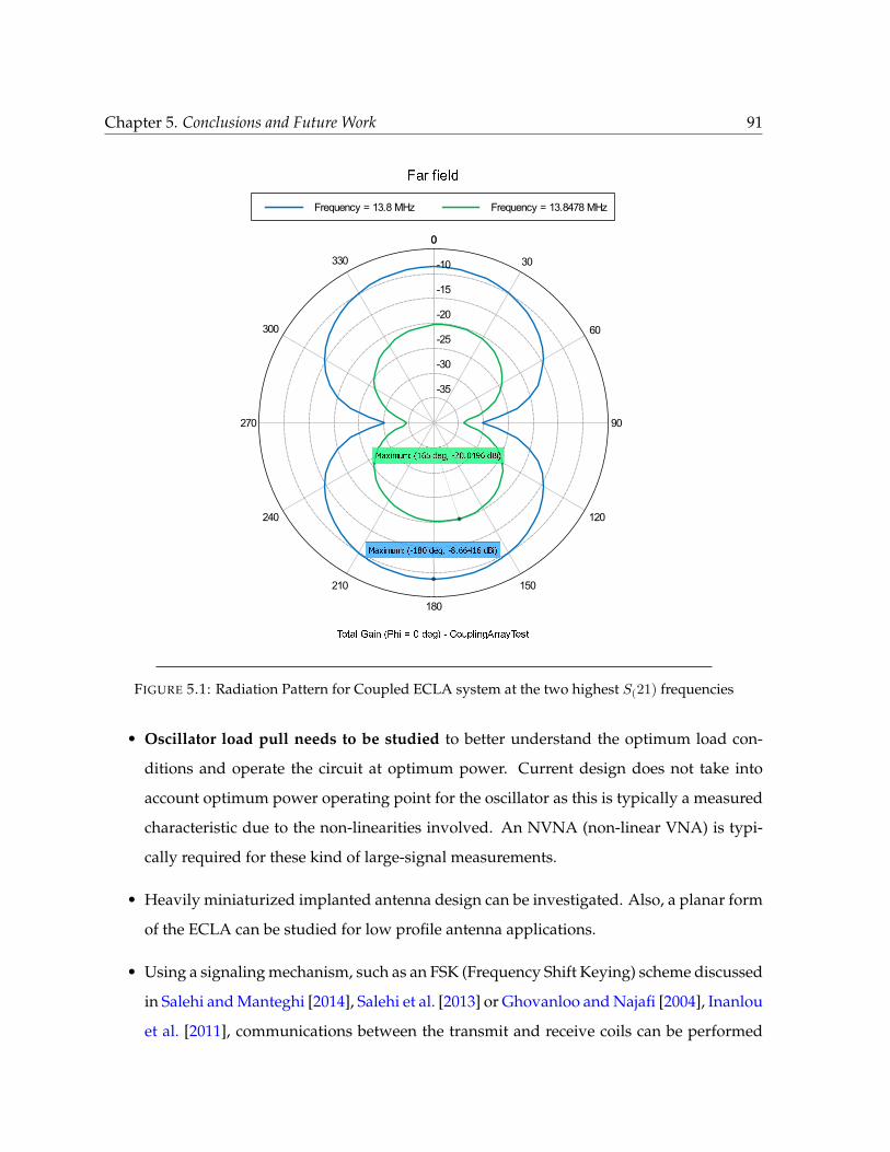
Chapter 5. Conclusions and Future Work 91
u.H
u.y
u=H
u=y
u H
u y
y
.y
zy
y
=y
Hy
y
= y
=My
=y
.yy
..y
y
55 .n5 55 .nM5
FIGURE 5.1: Radiation Pattern for Coupled ECLA system at the two highest S(21) frequencies
• Oscillator load pull needs to be studied to better understand the optimum load con-
ditions and operate the circuit at optimum power. Current design does not take into
account optimum power operating point for the oscillator as this is typically a measured
characteristic due to the non-linearities involved. An NVNA (non-linear VNA) is typi-
cally required for these kind of large-signal measurements.
• Heavily miniaturized implanted antenna design can be investigated. Also, a planar form
of the ECLA can be studied for low profile antenna applications.
• Using a signaling mechanism, such as an FSK (Frequency Shift Keying) scheme discussed
in Salehi and Manteghi [2014], Salehi et al. [2013] or Ghovanloo and Najafi [2004], Inanlou
et al. [2011], communications between the transmit and receive coils can be performed

Chapter 5. Conclusions and Future Work 92
without the need of another wireless channel (as in the case of Rezence and other com-
mercial offerings), thus minimizing cost.
• Adaptive frequency and impedance control can be explored to maximize efficiency [Ping
et al., 2008, Poon et al., 2007, Sample et al., 2013].

Bibliography
Arbabi, A. and Safavi-Naeini, S. (2012). Maximum gain of a lossy antenna. Antennas and
Propagation, IEEE Transactions on, 60(1):2–7.
Azad, U., Jing, H. C., and Wang, Y. E. (2012). Link budget and capacity performance of induc-
tively coupled resonant loops. Antennas and Propagation, IEEE Transactions on, 60(5):2453–
2461.
Brown, W. C. (1996). The history of wireless power transmission. Solar energy, 56(1):3–21.
Catrysse, M., Hermans, B., and Puers, R. (2004). An inductive power system with integrated
bi-directional data-transmission. Sensors and Actuators A: Physical, 115(2):221–229.
Chu, L. J. (1948). Physical limitations of omni-directional antennas. Journal of applied physics,
19(12):1163–1175.
Collin, R. and Rothschild, S. (1964). Evaluation of antenna q. Antennas and Propagation, IEEE
Transactions on, 12(1):23–27.
Commission, E. R. (1995). Human exposure to electromagnetic fields, high frequency (10 khz
to 300 ghz).
Davis, W., Yang, T., Caswell, E., and Stutzman, W. (2011). Fundamental limits on antenna size:
a new limit. Microwaves, Antennas & Propagation, IET, 5(11):1297–1302.
Federal Communications Commission, U. (1996). In the matter of guidelines for evaluating the
environmental effects of radiofrequency radiation.
93

Bibliography 94
Fotopoulou, K. and Flynn, B. W. (2006). Wireless powering of implanted sensors using rf
inductive coupling. In Sensors, 2006. 5th IEEE Conference on, pages 765–768.
Gabriel, C., Gabriel, S., and Corthout, E. (1996). The dielectric properties of biological tissues:
I. literature survey. Physics in medicine and biology, 41(11):2231.
Ghovanloo, M. and Najafi, K. (2004). A wideband frequency-shift keying wireless link for
inductively powered biomedical implants. Circuits and Systems I: Regular Papers, IEEE Trans-
actions on, 51(12):2374–2383.
Ghovanloo, M. and Najafi, K. (2007). A wireless implantable multichannel microstimulating
system-on-a-chip with modular architecture. Neural Systems and Rehabilitation Engineering,
IEEE Transactions on, 15(3):449–457.
Gonzalez, G. (1984). Microwave transistor amplifiers: analysis and design, volume 61. Prentice-
Hall Englewood Cliffs, NJ.
Grebennikov, A. (2007). RF and microwave transistor oscillator design. John Wiley & Sons.
Guoxing, W., Wentai, L., Sivaprakasam, M., and Kendir, G. A. (2005). Design and analysis of
an adaptive transcutaneous power telemetry for biomedical implants. Circuits and Systems I:
Regular Papers, IEEE Transactions on, 52(10):2109–2117.
Hall, P. S. and Hao, Y. (2006). Antennas and propagation for body centric communications. In
Antennas and Propagation, 2006. EuCAP 2006. First European Conference on, pages 1–7. IEEE.
Harrington, R. F. (1960). Effect of antenna size on gain, bandwidth, and efficiency. J. Res. Nat.
Bur. Stand, 64(1):1–12.
Haus, H. A. et al. (1984). Waves and fields in optoelectronics, volume 464. Prentice-Hall Engle-
wood Cliffs, NJ.
Heebl, J. D., Thomas, E. M., Penno, R. P., and Grbic, A. (2014). Comprehensive analysis
and measurement of frequency-tuned and impedance-tuned wireless non-radiative power-
transfer systems. Antennas and Propagation Magazine, IEEE, 56(4):44–60.

Bibliography 95
Hong, J.-S. G. and Lancaster, M. J. (2004). Microstrip filters for RF/microwave applications, volume
167. John Wiley & Sons.
Hui, S., Zhong, W., and Lee, C. (2013). A critical review of recent progress in mid-range wireless
power transfer.
Ibraheem, A. and Manteghi, M. (2014a). Path loss inside human body using electrically cou-
pled loop antenna at different frequency bands. In Antennas and Propagation Society Interna-
tional Symposium (APSURSI), 2014 IEEE, pages 977–978.
Ibraheem, A. A. Y. and Manteghi, M. (2014b). Performance of an implanted electrically coupled
loop antenna inside human body. Progress In Electromagnetics Research, 145:195–202.
IEEE (2010). Ieee standard for safety levels with respect to human exposure to radio frequency
electromagnetic fields, 3 khz to 300 ghz - amendment 1: Specifies ceiling limits for induced
and contact current, clarifies distinctions between localized exposure and spatial peak power
density. IEEE Std C95.1a-2010 (Amendment to IEEE Std C95.1-2005), pages C1–9.
Inanlou, F., Kiani, M., and Ghovanloo, M. (2011). A 10.2 mbps pulse harmonic modula-
tion based transceiver for implantable medical devices. Solid-State Circuits, IEEE Journal of,
46(6):1296–1306.
Jin, J.-M. (2011). Theory and computation of electromagnetic fields. John Wiley & Sons.
Jungsuek, O. and Sarabandi, K. (2012). Low profile, miniaturized, inductively coupled capaci-
tively loaded monopole antenna. Antennas and Propagation, IEEE Transactions on, 60(3):1206–
1213.
Karalis, A., Joannopoulos, J. D., and Soljacic, M. (2008). Efficient wireless non-radiative mid-
range energy transfer. Annals of Physics, 323(1):34–48.
Karalis, A., Kurs, A., Moffatt, R., Joannopoulos, J., Fisher, P., and Soljacic, M. (2010). Wireless
power range increase using parasitic resonators. US Patent App. 12/787,765.
Karlsson, A. (2004). Physical limitations of antennas in a lossy medium. Antennas and Propaga-
tion, IEEE Transactions on, 52(8):2027–2033.

Bibliography 96
Kiani, M. and Ghovanloo, M. (2012). The circuit theory behind coupled-mode magnetic
resonance-based wireless power transmission. Circuits and Systems I: Regular Papers, IEEE
Transactions on, 59(9):2065–2074.
Kiani, M. and Ghovanloo, M. (2013). A figure-of-merit for designing high-performance induc-
tive power transmission links. Industrial Electronics, IEEE Transactions on, 60(11):5292–5305.
Kiani, M., Jow, U.-M., and Ghovanloo, M. (2011). Design and optimization of a 3-coil inductive
link for efficient wireless power transmission. Biomedical Circuits and Systems, IEEE Transac-
tions on, 5(6):579–591.
Kim, H.-S., Won, D.-H., and Jang, B.-J. (2010). Simple design method of wireless power transfer
system using 13.56 mhz loop antennas. In Industrial Electronics (ISIE), 2010 IEEE International
Symposium on, pages 1058–1063. IEEE.
Kim, J. and Rahmat-Samii, Y. (2004). Implanted antennas inside a human body: Simula-
tions, designs, and characterizations. Microwave Theory and Techniques, IEEE Transactions on,
52(8):1934–1943.
Kim, K. (2012). Wireless Power Transfer: Principles and Engineering Explorations. Intech.
King, R. W. P., Smith, G. S., Owens, M., and Wu, T. T. (1981). Antennas in matter: Fundamen-
tals, theory, and applications. NASA STI/Recon Technical Report A, 81:29690.
Kumar, A., Mirabbasi, S., and Mu, C. (2009). Resonance-based wireless power delivery for
implantable devices. In Biomedical Circuits and Systems Conference, 2009. BioCAS 2009. IEEE,
pages 25–28.
Kurokawa, K. (1969). Some basic characteristics of broadband negative resistance oscillator
circuits. Bell System Technical Journal, 48(6):1937–1955.
Kurs, A., Karalis, A., Moffatt, R., Joannopoulos, J. D., Fisher, P., and Soljacic, M. (2007). Wireless
power transfer via strongly coupled magnetic resonances. science, 317(5834):83–86.
Large, D., Ball, L., and Farstad, A. (1973). Radio transmission to and from underground coal
mines–theory and measurement. Communications, IEEE Transactions on, 21(3):194–202.

Bibliography 97
Lee, K. and Cho, D. (2015). Analysis of wireless power transfer for adjustable power distribu-
tion among multiple receivers.
Lee, K. and Cho, D.-H. (2013). Diversity analysis of multiple transmitters in wireless power
transfer system. Magnetics, IEEE Transactions on, 49(6):2946–2952.
Manteghi, M. (2013a). Electrically coupled loop antenna as a dual for the planar inverted-f
antenna. Microwave and Optical Technology Letters, 55(6):1409–1412.
Manteghi, M. (2013b). A new resonator for high efficiency wireless power transfer. In Antennas
and Propagation Society International Symposium (APSURSI), 2013 IEEE, pages 838–839. IEEE.
Manteghi, M. and Ibraheem, A. (2014). On the study of the near-fields of electric and magnetic
small antennas in lossy media.
McLean, J. S. (1996). A re-examination of the fundamental limits on the radiation q of electri-
cally small antennas. Antennas and Propagation, IEEE Transactions on, 44(5):672.
Mohammadian, A. (2009). Method and apparatus with negative resistance in wireless power
transfers. US Patent App. 12/266,525.
Nambiar, S. C. and Manteghi, M. (2014a). A simple wireless power transfer scheme for im-
planted devices. In Radio Science Meeting (USNC-URSI NRSM), 2014 United States National
Committee of URSI National, pages 1–1. IEEE.
Nambiar, S. C. and Manteghi, M. (2014b). Study of coupling efficiency of wireless power trans-
fer systems in implanted applications. In Antennas and Propagation Society International Sym-
posium (APSURSI), 2014 IEEE, pages 842–843. IEEE.
Neihart, N. M. and Harrison, R. R. (2005). Micropower circuits for bidirectional wireless
telemetry in neural recording applications. Biomedical Engineering, IEEE Transactions on,
52(11):1950–1959.
Ping, S., Hu, A. P., Malpas, S., and Budgett, D. (2008). A frequency control method for regulat-
ing wireless power to implantable devices. Biomedical Circuits and Systems, IEEE Transactions
on, 2(1):22–29.

Bibliography 98
Pollock, C. R. (1995). Fundamentals of optoelectronics. Irwin Chicago.
Poon, A. S., O’Driscoll, S., and Meng, T. H. (2007). Optimal operating frequency in wireless
power transmission for implantable devices. In Engineering in Medicine and Biology Society,
2007. EMBS 2007. 29th Annual International Conference of the IEEE, pages 5673–5678. IEEE.
RamRakhyani, A. K. and Lazzi, G. (2013). On the design of efficient multi-coil telemetry system
for biomedical implants. Biomedical Circuits and Systems, IEEE Transactions on, 7(1):11–23.
RamRakhyani, A. K., Mirabbasi, S., and Mu, C. (2011). Design and optimization of resonance-
based efficient wireless power delivery systems for biomedical implants. Biomedical Circuits
and Systems, IEEE Transactions on, 5(1):48–63.
Rhea, R. W. (1995). Oscillator design and computer simulation. Noble Publishing.
Salehi, M. and Manteghi, M. (2014). Self-contained compact transmitter for high-rate data
transmission. Electronics Letters, 50(4):316–318.
Salehi, M., Manteghi, M., Suh, S.-Y., Sajuyigbe, S., and Skinner, H. G. (2013). A wide-
band frequency-shift keying modulation technique using transient state of a small antenna.
Progress In Electromagnetics Research, 143:421–445.
Sample, A. P., Waters, B. H., Wisdom, S. T., and Smith, J. R. (2013). Enabling seamless wireless
power delivery in dynamic environments. Proceedings of the IEEE, 101(6):1343–1358.
Si, P., Hu, A. P., Hsu, J. W., Chiang, M., Wang, Y., Malpas, S., and Budgett, D. (2007). Wireless
power supply for implantable biomedical device based on primary input voltage regulation.
In Industrial Electronics and Applications, 2007. ICIEA 2007. 2nd IEEE Conference on, pages 235–
239.
Smith, G. S. (1984). Directive properties of antennas for transmission into a material half-space.
Antennas and Propagation, IEEE Transactions on, 32(3):232–246.
Taga, T. and Tsunekawa, K. (1987). Performance analysis of a built-in planar inverted antenna
for 800 mhz band portable radio units. Selected Areas in Communications, IEEE Journal on,
5(5):921–929.

Bibliography 99
Tesla, N. (1900). Apparatus for transmission of electrical energy. US Patent 649,621.
Tesla, N. (1914). Apparatus for transmitting electrical energy. US Patent 1,119,732.
Toncich, S., Ozaki, E., and Mohammadian, A. (2009). Method and apparatus for adaptive
tuning of wireless power transfer. US Patent App. 12/266,522.
Villamil, C. and Manteghi, M. (2013). A circuit model for the pifa. In Antennas and Propagation
Society International Symposium (APSURSI), 2013 IEEE, pages 702–703.
Wait, J. R. (1952). The magnetic dipole antenna immersed in a conducting medium. Proceedings
of the IRE, 40(10):1244–1245.
Wang, G., Liu, W., Sivaprakasam, M., Zhou, M., Weiland, J. D., and Humayun, M. S. (2006).
A dual band wireless power and data telemetry for retinal prosthesis. In Engineering in
Medicine and Biology Society, 2006. EMBS’06. 28th Annual International Conference of the IEEE,
pages 4392–4395. IEEE.
Wei, X., Wang, Z., and Dai, H. (2014). A critical review of wireless power transfer via strongly
coupled magnetic resonances. Energies, 7(7):4316–4341.
Wheeler, H. (1958). Fundamental limitaions of a small vlf antenna for submarines. Antennas
and Propagation, IRE Transactions on, 6(1):123–125.
Wheeler, H. A. (1947). Fundamental limitations of small antennas. Proceedings of the IRE,
35(12):1479–1484.
Wheeler, H. A. (1959). The radiansphere around a small antenna. Proceedings of the IRE,
47(8):1325–1331.
Wheeler, H. A. (1975). Small antennas. Antennas and Propagation, IEEE Transactions on,
23(4):462–469.
Xiaoyu, L., Fei, Z., Hackworth, S. A., Sclabassi, R. J., and Mingui, S. (2009). Wireless power
transfer system design for implanted and worn devices. In Bioengineering Conference, 2009
IEEE 35th Annual Northeast, pages 1–2.

Bibliography 100
Zierhofer, C. M. and Hochmair, E. S. (1996). Geometric approach for coupling enhancement of
magnetically coupled coils. Biomedical Engineering, IEEE Transactions on, 43(7):708–714.
Zimmerman, T. G. (1996). Personal area networks: near-field intrabody communication. IBM
systems Journal, 35(3.4):609–617.

Appendix A
ADS Techniques
A.1 Introduction
Keysight (Agilent) ADS has been an indispensable tool for studying the various aspects of this
thesis. A Test Bench Creation tool for optimization of the equivalent circuits is shown in the
first section followed by some tutorial links for studying non-linear techniques that the author
found helpful.
A.2 Test Bench Creation for Equivalent Circuit Optimization
To facilitate a semi-automated approach to computing the equivalent circuit parameters for an
ECLA (or any antenna in general), the author created the following setup for fast iteration. The
following technique allows one to create a model for a device and optimize parameters to fit
measurement data.
The hierarchy is as: Device model – Test Bench (TB) – Test Lab (TL) to compare model with
measurement. Note that the model can contain only pins and no ports. TB can contain
ports that are referenced in TL. A Sequencer can be used to test multiple TBs one after the
other. An Optimization routine takes care of minimizing the difference in the two TBs. Use
101
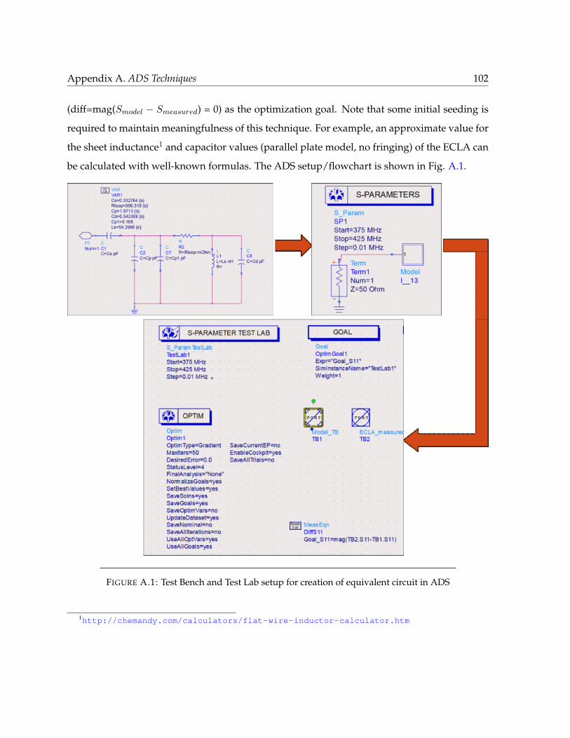
Appendix A. ADS Techniques 102
(diff=mag(Smodel − Smeasured) = 0) as the optimization goal. Note that some initial seeding is
required to maintain meaningfulness of this technique. For example, an approximate value for
the sheet inductance1 and capacitor values (parallel plate model, no fringing) of the ECLA can
be calculated with well-known formulas. The ADS setup/flowchart is shown in Fig. A.1.
FIGURE A.1: Test Bench and Test Lab setup for creation of equivalent circuit in ADS
1http://chemandy.com/calculators/flat-wire-inductor-calculator.htm

Appendix A. ADS Techniques 103
A.3 ADS Non-Linear and General Techniques References
Given below are some useful repositories and/or direct links to ADS techniques that can be
found freely on the internet.
• Prof. Long’s notes: http://www.ece.ucsb.edu/˜long/ece145a/
• Prof. Rodwell’s notes on oscillator design: http://www.ece.ucsb.edu/Faculty/
rodwell/Classes/ece218b/notes/OscSim.pdf
• Prof. Henderson’s notes: https://www.utdallas.edu/˜rmh072000/Site/Software_
and_Links_files/

Appendix B
MATLAB Codes
B.1 Introduction
Along Chapters 2 and 4, some of the computational work has been done through the use ofMATLAB code. They may be found below.
B.2 FEKO Field Extraction and Plotting
B.2.1 NormalizedPowerPlotter.m
%% Dipole data plotting tool: Plots Normalized power ratios for E/MDipoles
% Author: Shyam C. Nambiar% Date: 04/09/2014% (c) 2015 All rights reserved with author.%% Initialize and setupclear all;close all;clc;delete *.dat;disp('All previous data files have been deleted!');% Theoretical Data Stored herenormPowerTh_dB=[22.6983 19.0519 16.4535 14.4399 12.8045 11.4367
10.2701 ...9.2612 8.3800 7.6047 6.9187 6.3091 5.7654 5.2792 4.84 4.45164.0990 ...3.7810 3.4937 3.2338 2.9982 2.7843 2.5898 2.4128 2.2513 2.10381.9688];
%% Number of samples in various coordinates for E, H field data% Ideally, both E and H fields should have same number of sample
points.% However, at minimum, number of radial samples and start, end limits% should be equal to ensure comparable results.% % Ideal dipole number of samples% n1e=100;n1h=100;% n2e=10;n2h=10;% n3e=10;n3h=10;% Physical antenna number of samples
104

Appendix B. MATLAB Codes 105
n1e=199;n1h=199;n2e=10;n2h=10;n3e=10;n3h=19;% Size limits of sphere containing antenna, 'a' vectora_min=1;a_max=14;a_inc=0.5;a=a_min:a_inc:a_max;l_a=length(a);% % Ideal dipole file names% E_file='dipole_sphericalNF_3';% M_file='loop_sphericalNF_3';% Physical antenna file namesE_file='dipole_sphericalNF_4';M_file='loop_sphericalNF_4';EP_n=zeros(l_a,n1e);MP_n=zeros(l_a,n1h);%% Load all data[EP_r(1,:) Er(1,:)]=fn_PowerDistance3(E_file,E_file,n1e,n2e,n3e);[MP_r(1,:) Mr(1,:)]=fn_PowerDistance3(M_file,M_file,n1h,n2h,n3h);if ˜isequal(Er,Mr)
msg='Position vector information on E and H fields do not match!';error(msg);
enddisp('Files loaded');% Replicating data on all other rowsEP_r=repmat(EP_r(1,:),l_a,1);MP_r=repmat(MP_r(1,:),l_a,1);% Normalize and storefor ii=1:l_a
% Padding ones on non-essential indices with small values% to ensure consistent length. Zero-padding causes trouble in dBscale.EP_n(ii,1:ii)=ones(1,length(1:ii));MP_n(ii,1:ii)=ones(1,length(1:ii));% Normalize each row to power level found at r=aEP_n(ii,ii:n1e)=EP_r(ii,ii:n1e)./EP_r(ii,ii);MP_n(ii,ii:n1h)=MP_r(ii,ii:n1h)./MP_r(ii,ii);
end% Convert P_n to dBEP_n_dB=10.*log10(EP_n);MP_n_dB=10.*log10(MP_n);%% Plot figuresclose all;power_limits=[-50 0];% For plotting only up to a = xx mmdisp_max_index=23;a_limits=[a(1) a(disp_max_index)];a_ticks=0:5:a(disp_max_index);a1=a(1:disp_max_index);EP_n_dB1=EP_n_dB(1:disp_max_index,1:10:n1e);MP_n_dB1=MP_n_dB(1:disp_max_index,1:10:n1h);c_ticks=-50:10:0;figure(1);surf(Er(1,1:10:n1e).*1E3,a1,EP_n_dB1);xlabel('Radiation distance, r (mm)');ylabel('Radius, a (mm)');zlabel('Normalized Radiated Power \itP_\itEˆ\itN (\itr,\ita
) (dB)');zlim(power_limits);ylim(a_limits);set(gca,'YTick',a_ticks)caxis(power_limits);view(39,12);hcb=colorbar;set(hcb,'YTick',c_ticks);figure(2);surf(Mr(1,1:10:n1e).*1E3,a1,MP_n_dB1);xlabel('Radiation distance, r (mm)');

Appendix B. MATLAB Codes 106
ylabel('Radius, a (mm)');zlabel('Normalized Radiated Power \itP_\itMˆ\itN (\itr,\ita
) (dB)');zlim(power_limits);ylim(a_limits);set(gca,'YTick',a_ticks)caxis(power_limits);view(39,12);hcb=colorbar;set(hcb,'YTick',c_ticks);figure(3);surf(a1,Mr(1,1:10:n1e).*1E3,(MP_n_dB1-EP_n_dB1)');ylabel('Radiation distance, r (mm)');set(gca,'XTick',a_ticks)xlabel('Radius, a (mm)');zlabel('Magnetic to Electric Normalized Power Ratio (dB)');view(39,12);colorbar;% load normPower_muscle_403_dB.mat;figure(4);plot(a,normPowerTh_dB,'-*b');grid on;hold on;plot(a,MP_n_dB(:,end)-EP_n_dB(:,end),'-or');xlabel('Radius, a (mm)');ylabel('Magnetic to Electric Normalized Power Ratio (dB)');legend('Theory','Simulation');hold off;disp('Figures plotted');%% All limits% figure(1);% surf(Er(1,1:10:n1e).*1E3,a,EP_n_dB(:,1:10:n1e));% xlabel('Radiation distance, r (mm)');% ylabel('Radius, a (mm)');% zlabel('Normalized Radiated Power \itP_\itEˆ\itN (\itr,\
ita) (dB)');% zlim(power_limits);% caxis(power_limits);% view(39,12);% colorbar;%% figure(2);% surf(Mr(1,1:10:n1e).*1E3,a,MP_n_dB(:,1:10:n1e));% xlabel('Radiation distance, r (mm)');% ylabel('Radius, a (mm)');% zlabel('Normalized Radiated Power \itP_\itMˆ\itN (\itr,\
ita) (dB)');% zlim(power_limits);% caxis(power_limits);% view(39,12);% colorbar;%% figure(3);% surf(a,Mr(1,1:10:n1e).*1E3,(MP_n_dB(:,1:10:n1e)-EP_n_dB(:,1:10:n1e)
)');% ylabel('Radiation distance, r (mm)');% xlabel('Radius, a (mm)');% zlabel('Magnetic to Electric Normalized Power Ratio (dB)');% view(39,12);% colorbar;%% % load normPower_muscle_403_dB.mat;% figure(4);% plot(a,normPowerTh_dB,'-*b');% grid on;% hold on;% plot(a,MP_n_dB(:,end)-EP_n_dB(:,end),'-or');% xlabel('Radius, a (mm)');% ylabel('Magnetic to Electric Normalized Power Ratio (dB)');% legend('Theory','Simulation');

Appendix B. MATLAB Codes 107
B.2.2 Functions
function [ P_abs, r ] = fn_PowerDistance3( file1, file2, n1, n2, n3 )%FN_POWERDISTANCE3 Given the filenames of E and H field data files,
number% of samples of each coordinate axis; returns Power wrt distance% (Resultant Power), Distance vector.% Resultant power, P_abs, is resultant of components of P_r.[˜,E]=fn_FEKO_FieldExtractor(file1,'.efe');[r_vec,H]=fn_FEKO_FieldExtractor(file2,'.hfe');S=fn_Power2(E,H);r=r_vec((1:n1).*n2.*n3,1);theta=r_vec((1:n2).*n3,2);phi=r_vec(1:n3,3);% If symmetrical solution used, multiply by factor to compute total
powerfactor1=1;factor2=1;if 180-theta(end)>5
factor1=180/theta(end);endif 360-phi(end)>10
factor2=360/phi(end);endfactor=factor1*factor2;P_r=zeros(n1,1);for rr=1:n1
term=0;a=r(rr);for tt=2:n2
dt=theta(tt)-theta(tt-1);for pp=2:n3
dp=phi(pp)-phi(pp-1);ind=(rr-1)*n2*n3+(tt-1)*n3;term=term+S(ind).*(aˆ2).*sin(theta(tt)).*dt.*dp;
endendP_r(rr)=term;
endP_r=factor.*P_r;P_abs=P_r;% P_abs=sqrt(sum(P_r.ˆ2,2));end
function [ r_vec, X ] = fn_FEKO_FieldExtractor( filename, ext )%FN_FEKO_FIELDEXTRACTOR Extracts the position vector and field
information%from a FEKO gnerated file% Input: filename and extension (.efe or .hfe) as strings% Output: Position vector and complex field componentssource=fopen([filename ext]);if exist([filename '.dat'],'file')
filename=[filename '(1)'];endtarget=fopen([filename '.dat'],'w');% Define number of header lines, 15 defaultnumHdrLines=15;for ii=1:numHdrLines
[˜]=fgets(source);endptr=ftell(source);% File pointer is at ptr for FEKO Field files after numHdrLinesfseek(source,ptr,-1);% Read from source file and write to another data filewhile ˜feof(source)
data=fgets(source);fwrite(target,data);
endfclose('all');dataFmt=load([filename '.dat']);dataFmt=sortrows(dataFmt);

Appendix B. MATLAB Codes 108
% Store position vector columnsr_vec=dataFmt(:,1:3);% Store Complex field valuesX(:,1)=dataFmt(:,4)+1j.*dataFmt(:,5);X(:,2)=dataFmt(:,6)+1j.*dataFmt(:,7);X(:,3)=dataFmt(:,8)+1j.*dataFmt(:,9);end
B.3 Stability Analysis, Negative Resistance Termination Network forOscillator Design
B.3.1 NegRes.m
%% Negative Resistance Termination Network Calculator% Author: Shyam C. Nambiar, VTAG, Virginia Tech% Date: 01/02/2015% (c) 2015 All rights reserved with author.%% Initclear all;clc;%Transistor S-params at required frequency (Must fill out)f=420.9E6;s=[0.99641 127.32;0.15043 -95.963;2.2414
86.852;1.1716 -161.03];s=fn_sPar_MA_AB(s);delta=fn_delta(s)K=fn_RollettStab(s,delta)% Few sample points to startgam_T=[1j,-1,-1j,0];gam_InP=fn_gamma_out(s,gam_T);abs(gam_InP)rad2deg(angle(gam_InP))%% Plot Stability Circles% Compute required valuesdisp('Magnitude of delta');disp(abs(delta));CL=( conj( s(2,2)-delta*(conj(s(1,1))) ) / ...
( (abs(s(2,2)))ˆ2 - (abs(delta))ˆ2 ) );RL=abs( ( s(1,2)*s(2,1) ) / ( (abs(s(2,2)))ˆ2 - (abs(delta))ˆ2 ) );CS=( conj( s(1,1)-delta*(conj(s(2,2))) ) / ...
( (abs(s(1,1)))ˆ2 - (abs(delta))ˆ2 ) );RS=abs( ( s(1,2)*s(2,1) ) / ( (abs(s(1,1)))ˆ2 - (abs(delta))ˆ2 ) );% Plot stability circlesfigure(1);hold on;unitO=fn_circle(0,1,'b');inpStabO=fn_circle(CL,RL,'r');outStabO=fn_circle(CS,RS,'g');legend('Unit Circle','Input/Load (\Gamma_outˆ\prime) Stability
Circle','Output/Terminating (\Gamma_inˆ\prime) Stability Circle');
axis equal;grid on;hold off;% disp('Magnitude of Gamma_in with CL');% disp(abs(fn_gamma_in(s,CL)));%% disp('Magnitude of Gamma_out with CS');% disp(abs(fn_gamma_out(s,CS)));%% Find optimum Gamma_InPrime or Gamma_OutNr=50;x=linspace(-1,1,Nr);y=linspace(-1,1,Nr);
Appendix B. MATLAB Codes 109
[X Y]=meshgrid(x,y);xcs=real(CS);ycs=imag(CS);idx1=find(sqrt((X-xcs).ˆ2+(Y-ycs).ˆ2)>RS);Gam_T_test=X+1j.*Y;Gam_InP_test=fn_gamma_out(s,Gam_T_test);Z=log10(abs(Gam_InP_test));%% Plot the values of Gamma_InPrime for various Gamma_T_testfigure(2);hold onpcolor(X,Y,Z);colormap(hot);colorbar;unitO=fn_circle(0,1,'w');outStabO=fn_circle(CS,RS,'g');axis equal;grid on;hold off;%% Given a specified load, design termination or vice versaZt=29.18-1j*4.16; % Input impedance of antenna% Zt=50; % Input impedance of antennaGam_T=fn_refFromImp(50,Zt)Gam_InP=fn_gamma_out(s,Gam_T);ZinP=fn_impFromRef(50,Gam_InP);Zl=-1*real(ZinP)/3 - 1j* imag(ZinP)% Value of reactive componentiZl=imag(Zl);if(iZl>0)
L=iZl/(2*pi*f)else
C=1/(iZl*2*pi*f)end
B.3.2 Functions
function [ s_ab ] = fn_sPar_MA_AB( s_ma )%FN_SPAR_MA_AB converts s matrix in magnitude phase form to a+jb formang_rad=degtorad(s_ma(:,2));for i=1:4
[x,y]=pol2cart(ang_rad(i),s_ma(i,1));temp(1,i)=x+1j*y;
ends_ab(1,:)=temp(1,1:2);s_ab(2,:)=temp(1,3:4);end% function [ s_ab ] = fn_sPar_MA_AB( s_ma )% %FN_SPAR_MA_AB converts s matrix in magnitude phase form to a+jb
form% ang_rad=degtorad(s_ma(:,2));% for i=1:4% [x,y]=pol2cart(ang_rad(i),s_ma(i,1));% temp=x+1j*y;% s_ab(floor(i/2) +1,mod(i+1,2) +1)=temp;% end% end
function delta=fn_delta(s)%FN_DELTA computes the delta value for given s paramter matrix% delta=s11*s22-s12*s21delta=s(1,1)*s(2,2)-s(1,2)*s(2,1);end
function K = fn_RollettStab(s,delta)%FN_ROLLETTSTAB computes the Rollett Stability Factor K for gien s-
matrix

Appendix B. MATLAB Codes 110
%and delta% K= ( 1 + (abs(delta))ˆ2 - (abs(s11))ˆ2 - (abs(s22))ˆ2)/(2*abs(s12
*s21))K= ( 1 + (abs(delta))ˆ2 - (abs(s(1,1)))ˆ2 - (abs(s(2,2)))ˆ2)/...
(2*abs(s(1,2)*s(2,1)));end
function gam_in = fn_gamma_in(s,gamma_l)%FN_GAMMA_IN computes the complex value of gamma_in for given s-
matrix and% load reflection coefficient 'gamma_l'% gam_in= s11 + (s12*s21*gamma_l)/(1-s22*gamma_l)gam_in = s(1,1) + ( s(1,2).*s(2,1).*gamma_l)./(1-s(2,2).*gamma_l);end
function gam_out = fn_gamma_out(s,gamma_s)%FN_GAMMA_OUT computes the complex value of gamma_out for given s-
matrix and% source reflection coefficient 'gamma_s'% gam_out= s22 + (s12*s21*gamma_s)/(1-s11*gamma_s)gam_out = s(2,2) + ( s(1,2).*s(2,1).*gamma_s)./(1-s(1,1).*gamma_s);end
function Z = fn_impFromRef(Z_0,gamma)%FN_IMPFROMREF computes the relevant source/load reflection% Z= Z_0 * (1+gamma)/(1-gamma)Z= Z_0 * (1+gamma)/(1-gamma);end
function h = fn_circle(c,r,col)%FN_CIRCLE plots a circle with centre 'c' and radius 'r' in the
complex%planeth = 0:pi/50:2*pi;x = r * cos(th) + real(c);y = r * sin(th) + imag(c);h=plot(x,y,col);end


