Designing Cyclic Appointment Schedules for Outpatient Clinics with

Scheduled and Unscheduled Patient Arrivals

Nikky Kortbeek · Maartje E. Zonderland · Richard J. Boucherie ·Nelly Litvak · Erwin W. Hans

Abstract We present a methodology to design appointment systems for outpatient clinics and diagnostic fa-

cilities that offer both walk-in and scheduled service. The developed blueprint for the appointment schedule

prescribes the number of appointments to plan per day and the moment on the day to schedule the appointments.

The method consists of two models that are linked by an algorithm; one for the day process that governs sched-

uled and unscheduled arrivals on the day and one for the access process of scheduled arrivals. Appointment

schedules that balance the waiting time at the facility for unscheduled patients and the access time for scheduled

patients, are calculated iteratively using the outcomes of the two models. The method is of general nature and

can therefore also be applied to scheduling problems in other sectors than health care.

Keywords Health Care Management; Service Operations; Production Planning and Scheduling; Queuing

Theory; Stochastic Methods

1 Introduction

Developing appointment schedules for service facilities that process both scheduled and unscheduled arrivals

is challenging, as it requires planning and scheduling on different time scales. A well-designed appointment

system comprises an efficient day appointment schedule and provides timely access. This paper is motivated

by challenges faced by hospital outpatient clinics that serve patients on a walk-in basis. Most of these clinics

also have a limited number of appointment slots. There are various organizational (e.g., fixed slots for patients

Nikky Kortbeek · Maartje E. Zonderland · Richard J. Boucherie · Nelly Litvak

Stochastic Operations Research & Center for Healthcare Operations Improvement and Research

University of Twente, Postbox 217, 7500 AE Enschede, the Netherlands

E-mail: n.kortbeek@utwente.nl · m.e.zonderland@lumc.nl

Nikky Kortbeek

Department of Quality and Process Innovation, Academic Medical Center Amsterdam

Meibergdreef 9, 1105 AZ Amsterdam, the Netherlands

Maartje E. Zonderland

Division I, Leiden University Medical Center

Postbox 9600, 2300 RC Leiden, the Netherlands

Erwin W. Hans

Operational Methods for Production and Logistics & Center for Healthcare Operations Improvement and Research

University of Twente, Postbox 217, 7500 AE Enschede, the Netherlands

2

in a care pathway, patients with long travel time to the hospital, children) and medical (e.g., local anesthesia or

contrast fluid required) reasons to give a patient an appointment. In this paper, we introduce a method to design

appointment schedules for such facilities.

Advantages of a walk-in system are a higher level of accessibility and more freedom for patients to choose the

date and time of their hospital visit. Disadvantages are a possible highly variable demand and as a consequence

low utilization and high waiting time (the time between the physical arrival at the facility and the start of con-

sultation and/or treatment). The advantage of an appointment system is that workload can be dispersed, while

it has the disadvantage of a potentially long access time (the time between the day of the appointment request

and the appointment date). Since prolonged access times result in a delay of treatment, deterioration of health

condition is a serious risk (Murray and Berwick 2003). Allowing patients to walk in effectively reduces access

times to zero, and thus increases quality of care. In addition, health care facilities typically aim to guarantee a

certain service level with respect to the access time for patients with an appointment.

The challenge in a mixed system is thus to balance access time for appointment patients and waiting time for

walk-in patients. To achieve this, we develop a methodology that schedules appointments when the expected

walk-in demand is low. To smoothen the system, in periods of high demand part of the walk-in patients is

offered an appointment at a later moment. Of course, this is undesirable since it increases access time and may

involve an additional clinic visit. Walk-in demand (Ashton et al. 2004, Cochran and Roche 2009) and demand

for appointments requests (Williams et al. 2010) are often cyclic; therefore, we develop a cyclic appointment

schedule. Appointment scheduling has received considerable attention in the literature (Section 2), as opposed

to the development of models that relate access and waiting time (Gupta and Denton 2008).

Our contribution is a methodology that incorporates unscheduled and scheduled arrivals and maximizes the

number of unscheduled patients served on the day of arrival, while satisfying a pre-specified access time norm

for scheduled patients. We model the unscheduled arrivals with a stochastic non-stationary arrival process and

incorporate balking behaviour. The scheduled patients have priority, may not show up, and appointment requests

are assumed to arrive according to a cyclic pattern. To account for the cyclic arrivals, the appointment schemes

we develop are also cyclic, where the cycle is a repeating sequence of days. The cycle length can, for instance,

be a week or a month. The cyclic appointment schedule (CAS) specifies a capacity cycle (the maximum number

of patients that can be scheduled on each day of the cycle) and a day schedule (the maximum number of patients

to be scheduled per time slot on each day). Access time and waiting time are measured on different time scales,

since access time is counted between days and waiting time during a day.

To facilitate the two time scales, our approach consists of decomposing the appointment planning process and

the service process during the day. For both processes we propose an analytical evaluation model. The first model

determines the access time for scheduled patients for any given capacity cycle. The second model determines

the expected number of unscheduled jobs that cannot be seen on the day of arrival. The two models are linked

by an iterative algorithm that stops when the CAS is found in which the fraction of unscheduled jobs seen on

the day of arrival is maximized, given that the restriction on the access time is satisfied. A numerical example of

a small problem instance demonstrates the potential of the methodology. In this example complete enumeration

is applied to find optimal day schedules. Our future research will aim at incorporating heuristics to quickly find

(close to) optimal day schedules, so that larger problem sizes can be tackled. Finding an optimal day schedule is

not straightforward and a field of research on its own (Cayirli and Veral 2003, Gupta and Denton 2008).

This paper is organized as follows. Section 2 provides a literature review. In Section 3, we give an introduction

to the methodology and provide a formal problem description. Sections 4-6 present the access and day process

evaluation models and the algorithm. Section 7 describes the numerical example, followed by the discussion and

conclusions in Section 8.

2 Literature

In many service facilities customers are requested to make an appointment. There is a substantial body of lit-

erature focusing on the design of appointment systems. Health care is the most prevalent application area and

hence also most considered in the literature (see the surveys by Cayirli and Veral (2003) and Gupta and Denton

3

(2008)). Appointment systems can be regarded as a combination of two distinct queueing systems. The first

queueing system concerns customers making an appointment and waiting until the day the appointment takes

place. The second queueing system concerns the process of a service session during a particular day. We denote

these two queueing processes as the ‘access process’ and the ‘day process’. The remainder of this section pro-

vides an overview of the literature relevant for the present work and is structured as follows: (1) appointment

scheduling, (2) access time models, and (3) integrating the access process and the day process.

2.1 Appointment scheduling

Appointment scheduling concerns designing blueprints for day-appointment schedules with typical objectives

as minimizing customer waiting time, and maximizing resource utilization or minimizing resource idle time. A

large part of the literature focuses on scheduling a given number of appointments on a particular day (e.g. Liao

et al. 1993, Liu and Liu 1998, Vanden Bosch et al. 1999, Kaandorp and Koole 2007). The extent to which various

aspects that impact the performance of an appointment schedule are incorporated varies, such as customer punc-

tuality (e.g. Lehaney et al. 1999), customers not showing up (’no-shows’) (e.g. Ho and Lau 1992, Kaandorp and

Koole 2007), lateness of the server at the start of a service session (e.g. Liu and Liu 1998), service interruptions

(e.g. Lehaney et al. 1999) and the variance of service duration (e.g. Ho and Lau 1992).

Research techniques employed in appointment scheduling can be divided in analytical and simulation-based

approaches, of which the latter is most widely applied (Cayirli and Veral 2003). In the day process we aim for an

analytical approach, namely finite time Markov chain analysis. Related examples with health care applications

are Pegden and Rosenshine (1990), Liao et al. (1993), Vanden Bosch et al. (1999), Kaandorp and Koole (2007)

and Hassin and Mendel (2008), although these references do not consider unscheduled customers.

Often, a homogeneous customer population is assumed (Creemers 2009). Some studies however, focus on ser-

vice systems with various customer types. Differentiation between customer types is identified as a consequence

of distinct service requirements (e.g. Klassen and Rohleder 1996, Wang 1999, Vanden Bosch et al. 1999, Van-

den Bosch and Dietz 2000, Cayirli et al. 2008). Also, distinct priority levels may be a reason for patient type

differentiation. An example can be found in Patrick and Puterman (2007), where service slots are premarked

for various scheduled customer classes. In this paper, customer type differentiation arises from distinct arrival

processes.

The effect of mixed arrival processes is studied in Green et al. (2006a), Kolisch and Sickinger (2008) and

Sickinger and Kolisch (2009). Here, scheduled outpatients, unscheduled inpatients and emergency patients are

taken into account. Patients without an appointment are either emergency patients who require non-preemptive

priority or inpatients available for ‘call-in’ at any time during the day. These unscheduled patients are assumed

to arrive according to an equal arrival rate throughout the day. In our case, we consider walk-in patients without

priority who cannot be called in during the day. Moreover, we consider non-stationary arrivals to incorporate the

expected peak behavior of walk-in demand. Studies that do incorporate non-priority unscheduled arrivals simi-

lar to the unscheduled arrivals in this paper are Reilly et al. (1978), Swisher et al. (2001), Su and Shih (2003),

Ashton et al. (2004), Cayirli et al. (2006), LaGanga and Lawrence (2007), Cayirli et al. (2008); however, in all

cases a simulation approach is employed. Also, these studies do not incorporate balking behavior of unscheduled

customers.

2.2 Access time models

As our approach consists of a decomposition, isolated access time models are also of interest. The access process

we consider is discrete-time and cyclical in both the arrival and service processes. Various access time models

based on continuous-time queueing models are available. Examples are the M(t)|M|s(t) queue Green and Soares

(2007) and the adapted M|M|s queue that models time-dependent demand Green et al. (2001). The latter method

is also applied to a health care problem in Green et al. (2006b). To preserve the discrete-time nature we take as

4

starting point the generating function approach for slotted queueing models in discrete time Bruneel and Wuyts

(1994). A survey on discrete-time queueing systems is presented in Bruneel (1993).

Models to evaluate the length of hospital waiting lists are introduced in Worthington (1987), and further studied

in for example Goddard and Tavakoli (2008). In these models homogeneous appointment request arrivals are

assumed. In polling models, multiple queues are served by one server in cyclic order (see Takagi (1988) for an

overview). However, cyclic arrival rates and cyclic service capacity have not yet been incorporated in polling

models.

2.3 Linking the access and the day process

We found only a few examples that jointly consider the access and day process. In Ramakrishnan et al. (2005)

the authors propose a two time scale model for the Emergency Department (ED) – Ward patient flow. The fast

time scale of the ED is modeled by a continuous time Markov chain, while the slower time scale of the wards is

modeled by a discrete time Markov chain. In Vanden Bosch and Dietz (2000) and Klassen and Rohleder (2004),

appointment schedules ranging over a horizon of several days are evaluated. The aim is to minimize the patient’s

waiting and the doctor’s idle time, but the patient’s access time is not studied in detail.

The advanced (or open) access methodology Murray and Berwick (2003) also considers two time scales. With

advanced access, a clinic leaves a fraction of appointment slots vacant for patients that request an appointment

on the same day or within a couple of days. As many patients as possible are scheduled on the day they make

an appointment request. One should determine the optimal ratio between the reserved capacity for long-term

and same-day appointments (Dobson et al. 2011). This principle is slightly adapted in Liu et al. (2010), where

the demand for short term appointments is distributed over several days, to smooth the daily load of the system.

The aim of the advanced access methodology is to minimize access time (“do today’s work today”). Note that

in an advanced access clinic patients do announce themselves in advance and make a (same-day) appointment,

contrary to the type of unscheduled patients we consider, who just show up. Models that study the advanced

access methodology usually focus on capacity distribution (e.g. Dobson et al. 2011, Qu et al. 2007, Qu and Shi

2009).

Formulating a model to design an appointment schedule considering two time scales is usually done using sim-

ulation techniques (e.g. (e.g. Kopach et al. 2007)). An analytic approach is presented in Patrick et al. (2008),

where the effect of capacity allocation among competing patient classes on access time targets is studied us-

ing techniques from Markov Decision Modeling and Mathematical Programming. An approach related to ours,

although without the presence of walk-in patients, is given in Creemers and Lambrecht (2010). The authors con-

sider a service facility, and first develop a vacation queuing system to determine the access time. Subsequently

an appointment system is developed that calculates the waiting time at the facility.

3 Formal Problem Description

This section defines all modeling assumptions, defines the CAS, formally states the research goal and gives an

overview of the proposed approach. Then, Sections 4 and 5 present two models to respectively evaluate the

access time to the facility and the day schedule performance. In Section 6, the two models are connected by

an algorithm, through which the best CAS is computed. Since our approach is generically applicable, we also

present the methodology in the generic terms: a facility that serves scheduled and unscheduled jobs.

Assumptions. A facility consisting of R resources is operational during T time slots of length h, during each

day in a cycle of D days. Two types of jobs have to be served: scheduled and unscheduled jobs. Service takes

one time slot. Scheduled jobs are given a specific date and time immediately when an appointment is requested.

In addition, when the facility is temporarily congested, unscheduled jobs are also offered an appointment: if

the service of an unscheduled job cannot start within g time slots after arrival, it will leave the facility and an

appointment will be planned for another day. We will refer to such jobs as deferred unscheduled jobs, or just

5

Table 1: Notation introduced in Section 3

Symbol Description

R Number of resources

T Number of time slots during a day

t Time slot index (t = 1, . . . ,T )

h Length of a time slot

D Cycle length in days

d Day index (d = 1, . . . ,D)

g Patience of an unscheduled job, expressed in the number of slots a job is willing to wait

λ d Initial appointment request arrival rate on day d

χdt Unscheduled job arrival rate on day d during time interval (t −1, t]

cdt Maximum number of appointments to schedule in slot t on day d

Cd Appointment schedule on day d, Cd = (cd1 , . . . ,c

dT )

C Cyclic appointment schedule, C = (C1, . . . ,CD)

kd Maximum number of appointments to schedule on day d

K Capacity cycle, K = (k1, . . . ,kD)

F E[Fraction of unscheduled jobs to serve at day of arrival during one cycle]

S(y) Access time service level: fraction of jobs with access time not greater than y

(y,Snorm(y)) Access time service level requirement: fraction of jobs with access time

not greater than y is at least S(y)

φ d Distribution of the number of deferred jobs on day d

γd Total appointment request arrival distribution on day d

νd Expected number of deferred jobs on day d

deferred jobs. The first available appointment slot for scheduled and deferred jobs is always the next day at the

earliest. All appointments, both scheduled jobs and deferred unscheduled jobs, are scheduled according to a First

Come First Served (FCFS) principle.

We assume a non-stationary Poisson process for the arrivals of appointment requests, with λ 1, . . . ,λ D the arrival

rates for different days in the cycle. Next, during each day in the cycle, we assume a non-stationary Poisson

arrival process for unscheduled job arrivals, with slot-dependent arrival rates: χdt for day d = 1, . . . ,D and time

slot t = 1, . . . ,T . Table 1 summarizes the notation introduced in this section.

Cyclic appointment schedule. To effectively counterbalance the non-stationarity at both the daily and cyclic (i.e.

weekly, biweekly or monthly) level, we aim to design an appointment schedule that is cyclic. We introduce the

CAS C = (C1, . . . ,CD), with Cd = (cd1 , . . . ,c

dT ), where cd

t specifies the maximum number of jobs that may be

scheduled in slot t on day d.

To find an adequate appointment schedule, we propose a decomposition. First, we introduce the concept of a

capacity cycle K = (k1, . . . ,kD), where kd prescribes the maximum number of jobs to schedule for day dD in the

cycle. Second, given the capacity cycle K, the day plan is specified. In order to match the capacity cycle K, the

day plan Cd should be such that kd = ∑Tt=1 cd

t .

Goal. An effective strategy balances the opportunities (1) for unscheduled jobs to be served on the same day

without long waiting time and (2) for scheduled jobs to be served within an acceptable access time. To this end,

we define the best policy as the cyclic appointment schedule in which the expected fraction of unscheduled jobs

served on the day of arrival, F , is maximized, while for scheduled jobs the access time service level, S(y), defined

as the percentage of jobs that is served within y days, is above a pre-specified norm Snorm(y). The value of the

vector (y,Snorm(y)) is chosen by the facility.

Approach. The best CAS is determined by employing an iterative algorithm that effectively utilizes our decom-

position of the CAS in the capacity cycle and the day plan. Figure 1 provides an overview of the algorithm.

In each iteration, first, capacity cycles are generated with at most R · T appointments per day, for which the

access time service level norm will be satisfied. All jobs requesting an appointment are taken into account –

thus both scheduled jobs and deferred unscheduled jobs. We derive the distribution of the number of deferred

6

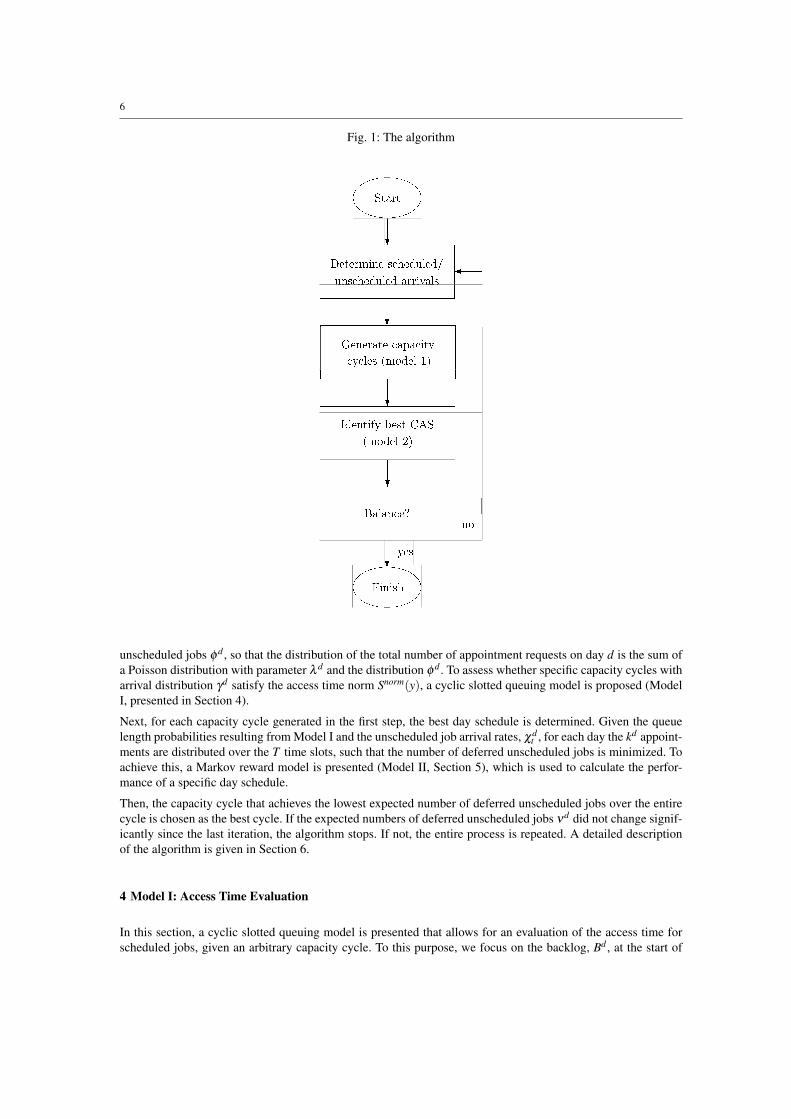
Fig. 1: The algorithm

unscheduled jobs φ d , so that the distribution of the total number of appointment requests on day d is the sum of

a Poisson distribution with parameter λ d and the distribution φ d . To assess whether specific capacity cycles with

arrival distribution γd satisfy the access time norm Snorm(y), a cyclic slotted queuing model is proposed (Model

I, presented in Section 4).

Next, for each capacity cycle generated in the first step, the best day schedule is determined. Given the queue

length probabilities resulting from Model I and the unscheduled job arrival rates, χdt , for each day the kd appoint-

ments are distributed over the T time slots, such that the number of deferred unscheduled jobs is minimized. To

achieve this, a Markov reward model is presented (Model II, Section 5), which is used to calculate the perfor-

mance of a specific day schedule.

Then, the capacity cycle that achieves the lowest expected number of deferred unscheduled jobs over the entire

cycle is chosen as the best cycle. If the expected numbers of deferred unscheduled jobs νd did not change signif-

icantly since the last iteration, the algorithm stops. If not, the entire process is repeated. A detailed description

of the algorithm is given in Section 6.

4 Model I: Access Time Evaluation

In this section, a cyclic slotted queuing model is presented that allows for an evaluation of the access time for

scheduled jobs, given an arbitrary capacity cycle. To this purpose, we focus on the backlog, Bd , at the start of

7

each day d. We define the backlog as the number of jobs for which a request for an appointment has already been

made, while the appointment itself has not yet taken place. We formulate a Lindley type equation to characterize

the backlog, and use a probability-generating function approach to derive expressions for the distribution of

the backlog at the start of each day in the cycle. From the backlog distribution, we will derive the access time

distribution. A summary of the notation used in this section is given in Table 2.

Lindley type equation. Consider day d. During the day, a maximum number of jobs, kd , is served, and a number

of new jobs, Ad , arrives. At the start of day d, there is a backlog Bd . Since it is not possible to make an appoint-

ment on the day of arrival itself, the backlog at the start of the next day equals the backlog on day d minus the

number of jobs served on day d plus the number of jobs that arrived on day d. This can be formalized in the

following Lindley type equation:

Bd+1 = (Bd − kd)++Ad ,

where (x)+ = x if x > 0, and 0 otherwise.

A Generating function approach. Using an approach based on generating functions (Bruneel and Wuyts 1994),

we derive expressions for the distribution of the backlog at the start of each day in the cycle. The transition

probabilities for going from state Bd = i to state Bd+1 = i′ are given by:

P

(Bd+1 = i′|Bd = i

)=

{P(Ad = i′

)if i− kd ≤ 0

P(Ad = i′− i+ kd

)if i− kd > 0.

Let πdj denote the stationary probability that at the start of day d, the backlog equals j jobs. Furthermore, let ad

j

denote the probability that Ad = j. Note that the underlying probability distribution does not necessarily has to

be Poisson. The stationary probabilities can be computed recursively, under the condition that the capacity for

scheduled jobs is larger than the average demand, i.e. ∑d E[Ad ] < ∑d kd , since otherwise we would be dealing

with an unstable system. For d = 1, . . . ,D, j ≥ 0 we obtain:

πd+1j = ad

j

kd−1

∑i=0

πdi +

j

∑q=0

adj−qπd

kd+q. (1)

We multiply both sides of (1) with the complex number z j, where |z| ≤ 1, and z j denotes z raised to the power j,

as opposed to index d in πdj , ad

j and kd . The summation of both sides of the resulting equation over j yields the

probability-generating function for πd+1:

PBd+1(z) =∞

∑j=0

πd+1j z j =

∞

∑j=0

(ad

j

kd−1

∑i=0

πdi +

j

∑q=0

adj−qπd

kd+q

)z j.

From this we obtain:

PBd+1(z) =∞

∑j=0

πd+1j z j = PAd(z)z

−kd

PBd(z)+PAd(z)z−kd

kd−1

∑i=0

πdi

(zkd

− zi).

Table 2: Notation introduced in Section 4

Symbol Description

Bd Backlog at start of day d

PBd (z) Generating function of Bd

Ad Number of appointment requests arriving at day d

adj Appointment request arrival probabilities, P

(Ad = j

)

PAd (z) Generating function of Ad

πdj Stationary backlog probabilities, P

(Bd = j

)

k Total number of available appointment slots in a capacity cycle, k = ∑d kd

E[W d ] E[Access time for an appointment request arriving at day d]

E[W ] E[Access time for an arbitrary appointment request]

8

Rearranging terms and changing the order of summation leads to the probability generating function of Bd :

PBd (z) =∑

Di=1 ∑

kd+D−i−1q=0 (zkd+D−i

− zq)πd+D−iq

[∏

d+D−i−1s=d zks

∏i−1r=0 PAd+D−r−1(z)

]

∏Dg=1 zkg

−∏Dh=1 PAh(z)

,

where, since we consider days in a repeating cycle, we define:

d :=

{D ,d mod D = 0

d mod D ,otherwise.

The generating functions uniquely determine the stationary probabilities πdj , j = 0, . . . ,kd − 1, d = 1, . . . ,D. To

calculate these probabilities, we build upon the approach given in Adan et al. (2006). Define k as the total

number of available appointment slots in a capacity cycle, i.e. k = ∑Dd=1 kd . Then, the denominator of PBd (z) has

k−1 zeros inside the unit disk; this can be shown by using Rouche’s theorem (Kleinrock 1975). All generating

functions, including PBd (z), are bounded for |z| ≤ 1, and therefore the zeros of the denominator are also zeros of

the numerator (Bruneel and Wuyts 1994). Thus we obtain k−1 equations, and use PBd (1) = 1 to secure the last

equation. The k−1 zeros of the denominator of PBd (z) can be found by solving:

D

∏g=1

zkg

−D

∏h=1

PAh(z) = 0. (2)

The solutions of (2) also represent zeros of the numerator. Together with the normalizing equation PBd (1) = 1,

PBd (z) is completely defined for d = 1, . . . ,D. Note that now only the backlog probabilities for j = 0, . . . ,kd −1,

have been derived. The remaining backlog probabilities are calculated directly using (1).

Performance measures. The access time distribution can be directly derived from the backlog probabilities, since

appointment requests are served according to the FCFS principle. The FCFS service order and the impossibility

of making an appointment request for the day of arrival results in an access time of at least one day. Several

performance measures can be derived. Of particular interest are the probability distribution of the access time,

the expected access time and the access time service level.

1. The probability distribution of the access time. First we derive the conditional access time probability that the

access time for a client arriving at day d exceeds y days, given that the backlog at the start of day d equals b

clients. As argued, for y = 0, we have that

P[W d > y|Bd = b] = 1 ∀b.

For y > 0, we have that

P[W d > y|Bd = b] =

{1 if b ≥ ∑

yi=0 kd+i

∑∞j=s+1( j−s)·P[Ad= j]

E[Ad ]otherwise,

(3)

where s represents the number of jobs arrived on day d that will be served within y days:

s = min

{y

∑i=1

kd+i,y

∑i=0

kd+i −b

}.

We can explain formula (3) as follows. First, when the backlog b outnumbers the available capacity in y days, the

conditional probability that the access time exceeds y days equals 1. Otherwise, all arrivals beyond the number

s will wait for more than y days. There are j− s such arrivals. Then, the probability that the access time for a

client arriving at day d exceeds y days, equals

P[W d > y] =∞

∑b=0

P[W d > y|Bd = b] ·P[Bd = b].

2. The expected access time. Analogously, the expected access time for an appointment request that arrives on

day d is computed with:

E[W d |Bd = b] =∞

∑y=0

P[W d > y|Bd = b],

9

and thus

E[W d ] =∞

∑b=0

E[W d |Bd = b] ·P[Bd = b],

and

E[W ] =D

∑d=1

E[W d ]E[Ad ]

∑Dq=1E[A

q].

3. The access time service level. Using the access time probability distribution, we determine the fraction of

scheduled jobs for which the access time does not exceed y. We define this as follows:

S(y) =D

∑d=1

(1−P[W d > y]

)E[Ad ]

∑Dq=1E[A

q].

5 Model II: day process evaluation

In this section, we present a model to evaluate the performance of a single day in the CAS. Recall that the CAS

consists of a capacity cycle, K = (k1, . . . ,kD), that prescribes the maximum number of jobs that can be scheduled

for day d. Using model I, we were able to evaluate the access time performance of a given capacity cycle. Below,

we evaluate the day process of a given appointment schedule, by formulating a Markov reward process.

Note that although day appointment schedule Cd is open for scheduling appointments, there may be less backlog

than the kd = ∑t cdt available appointment slots. Therefore, we introduce the notation Cd to represent the realized

day planning, which is the schedule we evaluate. Now, Cd =(cd

1 , . . . , cdT

)expresses the actually utilized appoint-

ment slots. Since appointments are planned on a FCFS basis, the realized appointment day schedule, Cd , will

always be a truncated version of the day schedule, Cd . Of course, unoccupied appointment slots can be used for

unscheduled jobs.

Since we will consider the day performance on a day-by-day basis, in the remainder of this section we drop the

superscript d for notational convenience. Table 3 provides a summary of the notation introduced in this section.

Assumptions. For clarity of presentation, some of the assumptions introduced in Section 3 are repeated. During

one day the facility of R resources is operational during T intervals of length h. Two types of jobs have to be

served: scheduled and unscheduled jobs. Service always takes one time slot of length h. At the beginning of each

Table 3: Notation introduced in Section 5

Symbol Description

C Realized schedule under CAS C, C = (C1, . . . ,CD),Cd =(cd

1 , . . . , cdT

)

q P(No-show of a scheduled job)

et Number of slots available for unscheduled jobs in the next

g intervals after time t

pst (s) P(Number of scheduled jobs arriving at the start of slot t = s)

put (u) P(Number of unscheduled jobs arriving during interval (t −1, t] = u)

P [(s,u)t+1 | (k, l)t ] Transition probability from state (t,k, l) to state (t +1,s,u)

Qt(s,u) P(Number of scheduled, unscheduled jobs waiting at start of slot t = s,u)

νt E[Number of deferred jobs in time interval (0, t]]

ν E[Total number of deferred jobs]

φt Distribution of the number of deferred jobs in time interval (t −1, t]

φ Distribution of the total number of deferred jobs

10

time slot, a service can start. If there are both scheduled and unscheduled jobs, scheduled jobs are given priority.

Overtime is not allowed.

Scheduled jobs arrive on time, according to the schedule C. In addition, we allow for no-shows, that is, the

probability that a scheduled job actually arrives at the facility equals 1− q, so that q represents the probability

that a job does not show up.

Unscheduled jobs arrive at the facility according to an inhomogeneous Poisson process with slot-dependent

arrival rate χt . If the service of an unscheduled job cannot start within g time slots after arriving, it will leave the

facility and an appointment will be planned for another day. We assume that the facility has no pre-knowledge

about potential no-shows. Therefore, an unscheduled job arriving during interval (t −1, t] will stay if –and only

if– the number of unscheduled jobs already waiting is strictly smaller than the minimum number of service slots

during the upcoming g intervals that are not utilized by scheduled jobs. The number of time slots anticipated to

be available for unscheduled jobs during the upcoming g intervals is denoted by et :

et =min{t+g−1,T}

∑j=t

(R− c j). (4)

States. The state of the system is denoted by the tuple (t,s,u), which specifies that at the beginning of time slot

t, s scheduled and u unscheduled jobs are present.

Transition probabilities. Let pst (s) denote the probability that s scheduled jobs arrive at the beginning of time

slot t. Since each no-show is assumed to occur independently, these probabilities are calculated as follows:

pst (s) =

{(ct

s

)(1−q)s(q)ct−s ,0 ≤ s ≤ ct

0 ,s > ct .

Let put (u) denote the probability that u unscheduled jobs arrive during time interval (t −1, t]. As specified, pu

t (u)is Poisson distributed with slot dependent parameter χt . Note that χ1 represents the arrival rate of unscheduled

jobs that arrive before the opening time of the facility. Furthermore, note that any distribution function put can be

used in the day process evaluation model. Therefore, for model I the assumption of a Poisson arrival process is

not strictly required.

Let P [(s,u)t+1 | (v,w)t ] denote the transition probability of jumping from state (t,v,w) to (t +1,s,u). Below we

specify these transition probabilities for all possible events. In Figure 2, the state space for an arbitrary time slot

t is displayed in which the seven different possible events (a)-(g) are indicated. The events can be separated in

three groups: first, cases (a)-(c) in which no scheduled job is served (v = 0), second, cases (d) and (e) in which

Fig. 2: Day process state space and events

w

v

(a)

(b) (d)

(e)(c) (g)

(f)

wȱ=ȱet

11

both scheduled and unscheduled jobs are served (v < R), and third, cases (f) and (g) in which only scheduled

jobs are served (v ≥ R). In the expressions below, 1IA represents the indicator function; 1IA = 1 if condition A is

satisfied, and 0 otherwise.

Case (a). v = w = 0; no job served:

P [(s,u)t+1 | (v,w)t ] = pst+1(s)pu

t+1(u).

Case (b). v = 0,0 < w ≤ et ; unscheduled job(s) served:

P [(s,u)t+1 | (v,w)t ] = pst+1(s)pu

t+1(u−w+min{R,w})1I(u≥w−min{R,w}).

Case (c). v = 0,w > et ; unscheduled job(s) served, unscheduled job(s) abandoned:

P [(s,u)t+1 | (v,w)t ] = pst+1(s)pu

t+1(u− et +R)1I(u≥et−R).

Case (d). v < R,w ≤ et ; scheduled and unscheduled job(s):

P [(s,u)t+1 | (v,w)t ] = pst+1(s)pu

t+1(u−w+min{(R− v),w})1I(u≥w−min{(R−v),w}).

Case (e). v < R,w > et ; scheduled and unscheduled job(s) served, unscheduled job(s) abandoned:

P [(s,u)t+1 | (v,w)t ] = pst+1(s)pu

t+1(u− et +R− v)1I(u≥et−R+v).

Case (f). v ≥ R,w ≤ et ; scheduled job(s) served:

P [(s,u)t+1 | (v,w)t ] = pst+1(s− v+R)pu

t+1(u−w)1I(s≥v−R)1I(u≥w).

Case (g). v ≥ R,w > et ; scheduled job(s) served, unscheduled job(s) abandoned:

P [(s,u)t+1 | (v,w)t ] = pst+1(s− v+R)pu

t+1(u− et)1I(s≥v−R)1I(u≥et ).

Performance measures. Let Qt(s,u) denote the probability that at the start of slot t there are s scheduled and u

unscheduled jobs present. Qt(s,u) can be calculated as follows:

Q1(s,u) = ps1(s) · pu

1(u).

For t = 2, ...,T :

Qt+1(s,u) = ∑v

∑w

Qt(v,w)P [(s,u)t+1 | (v,w)t ] .

The expected number of deferred jobs ν = νT is calculated accordingly:

ν1 =∞

∑s=0

∞

∑u=e1+1

(u− e1) ·Q1(s,u).

For t = 2, ...,T :

νt = νt−1 +∞

∑s=0

∞

∑u=et+1

(u− et) ·Qt(s,u).

The distribution of the number of deferred jobs, φ , can be calculated as follows. For t = 1, . . . ,T :

φt( j) =

∞

∑s=0

et

∑u=0

Qt(s,u) , j = 0

∞

∑s=0

Qt(s,et + j) , j > 0,

and

φ = φ1 ∗ . . .∗φT ,

where ∗ denotes the discrete convolution function.

Remark 1 Clearly, other performance measures that might be of interest, such as waiting time and utilization

indicators, can also be calculated. Since in the algorithm of the next section, we will minimize the number of

deferred jobs, we restricted ourselves here to the calculation of this performance measure.

12

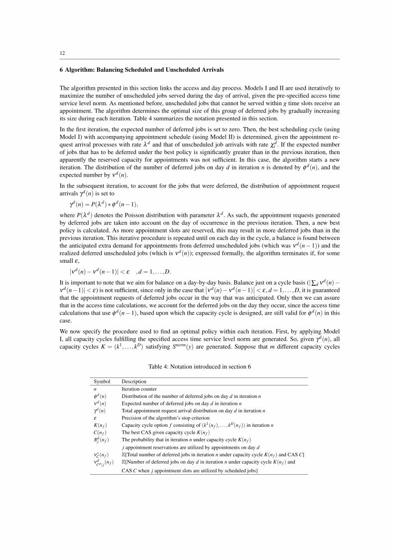
6 Algorithm: Balancing Scheduled and Unscheduled Arrivals

The algorithm presented in this section links the access and day process. Models I and II are used iteratively to

maximize the number of unscheduled jobs served during the day of arrival, given the pre-specified access time

service level norm. As mentioned before, unscheduled jobs that cannot be served within g time slots receive an

appointment. The algorithm determines the optimal size of this group of deferred jobs by gradually increasing

its size during each iteration. Table 4 summarizes the notation presented in this section.

In the first iteration, the expected number of deferred jobs is set to zero. Then, the best scheduling cycle (using

Model I) with accompanying appointment schedule (using Model II) is determined, given the appointment re-

quest arrival processes with rate λ d and that of unscheduled job arrivals with rate χdt . If the expected number

of jobs that has to be deferred under the best policy is significantly greater than in the previous iteration, then

apparently the reserved capacity for appointments was not sufficient. In this case, the algorithm starts a new

iteration. The distribution of the number of deferred jobs on day d in iteration n is denoted by φ d(n), and the

expected number by νd(n).

In the subsequent iteration, to account for the jobs that were deferred, the distribution of appointment request

arrivals γd(n) is set to

γd(n) = P(λ d)∗φ d(n−1),

where P(λ d) denotes the Poisson distribution with parameter λ d . As such, the appointment requests generated

by deferred jobs are taken into account on the day of occurrence in the previous iteration. Then, a new best

policy is calculated. As more appointment slots are reserved, this may result in more deferred jobs than in the

previous iteration. This iterative procedure is repeated until on each day in the cycle, a balance is found between

the anticipated extra demand for appointments from deferred unscheduled jobs (which was νd(n− 1)) and the

realized deferred unscheduled jobs (which is νd(n)); expressed formally, the algorithm terminates if, for some

small ε ,

|νd(n)−νd(n−1)|< ε ,d = 1, . . . ,D.

It is important to note that we aim for balance on a day-by-day basis. Balance just on a cycle basis (|∑d νd(n)−νd(n−1)|< ε) is not sufficient, since only in the case that

∣∣νd(n)−νd(n−1)∣∣< ε , d = 1, . . . ,D, it is guaranteed

that the appointment requests of deferred jobs occur in the way that was anticipated. Only then we can assure

that in the access time calculations, we account for the deferred jobs on the day they occur, since the access time

calculations that use φ d(n−1), based upon which the capacity cycle is designed, are still valid for φ d(n) in this

case.

We now specify the procedure used to find an optimal policy within each iteration. First, by applying Model

I, all capacity cycles fulfilling the specified access time service level norm are generated. So, given γd(n), all

capacity cycles K = (k1, . . . ,kD) satisfying Snorm(y) are generated. Suppose that m different capacity cycles

Table 4: Notation introduced in section 6

Symbol Description

n Iteration counter

φ d(n) Distribution of the number of deferred jobs on day d in iteration n

νd(n) Expected number of deferred jobs on day d in iteration n

γd(n) Total appointment request arrival distribution on day d in iteration n

ε Precision of the algorithm’s stop criterion

K(n f ) Capacity cycle option f consisting of (k1(n f ), . . . ,kD(n f )) in iteration n

C(n f ) The best CAS given capacity cycle K(n f )

πdj (n f ) The probability that in iteration n under capacity cycle K(n f )

j appointment reservations are utilized by appointments on day d

ν∗C(n f ) E[Total number of deferred jobs in iteration n under capacity cycle K(n f ) and CAS C]

νdCd | j

(n f ) E[Number of deferred jobs on day d in iteration n under capacity cycle K(n f ) and

CAS C when j appointment slots are utilized by scheduled jobs]

13

satisfy the norm, then denote these options for iteration n by K(n f ) = (k1(n f ), . . . ,kD(n f )), f = 1, . . . ,m. From

these options, the best capacity cycle is selected, which is the capacity cycle that minimizes the expected number

of deferred jobs. To do this, for each scheduling cycle option K(n f ), the best CAS C(n f ) is determined.

The best CAS’s are determined by applying Model II as follows. First, observe that although in a capacity cycle

K(n f ) there are kd(n f ) appointment slots reserved on day d, not all of these reserved slots are necessarily utilized

by scheduled jobs. Since appointments are planned according to the FCFS principle, we know from the queue

length probability vectors πd(n f ) of Model I, the probabilities of utilizing the first j out of the kd(n f ) reservations

under capacity cycle K(n f ). Let us denote these probabilities by πdj (n f ):

πdj (n f ) =

{πd

j (n f ) , j = 0, . . . ,kd(n f )−1

∑∞q=kd(n f )

πdq (n f ) , j = kd(n f ).

By evaluating each day appointment schedule for d = 1, . . . ,D, f = 1, . . . ,m and j = 0, . . . ,kd(n f ), the best CAS

is determined for each capacity cycle K(n f ), so by complete enumeration. Denote the expected total number of

deferred jobs in cycle K(n f ) under appointment schedule C by νC(n f ). With ν∗(n f ) defined as the expected total

number of deferred jobs in cycle K(n f ), under the best CAS the best cyclic appointment schedules are those that

minimize:

ν∗(n f ) = minC

νC(n f ) = minC

D

∑d=1

kd(n f )

∑j=0

πdj (n f )νd

Cd | j(n f ),

where νdCd | j

(n f ) denotes the expected number of deferred jobs on day d under capacity cycle K(n f ) and cyclic

appointment schedule C, if j appointment slots are utilized by scheduled jobs. Note that Cd | j is a truncated

version of Cd , in exactly the same way that Cd was defined in Section 5. Now, the final step is to select the

capacity cycle K(n f ) and accompanying CAS, which is the CAS with the lowest expected number of deferred

jobs, namely:

ν∗(n) = minf

ν∗(n f ) , f ∗(n) = argminf

ν∗(n f ) , C∗(n) = argminC

νC(n f ∗).

Figure 3 displays the complete algorithm in pseudocode.

Remark 2 (Convergence) For the system to be stable we require that ∑d λ d +∑d ∑t χdt < R · T , so that total

demand does not exceed capacity. In addition, we would like to determine the conditions under which the al-

gorithm will converge. Therefore, first observe that since the unscheduled job arrival rate χdt is fixed and the

first iteration starts with no deferred jobs, i.e. νd(0) = 0, in each iteration it is not possible to choose the CAS

Fig. 3: The algorithm

Step 1: Specify: R,T,D,g,q,Snorm(y),ε;

specify input ∀d : λ d ; ∀d, t : χdt .

Step 2: n := 1; ∀d : νd(1) := 0,γd(1) := P(λ d).initialize algorithm

Step 3: Given γd(n), determine all K(n f ), f = 1, . . . ,m,determine feasible cycles such that S(y)≥ Snorm(y). ∀ f ,d : store πd(n f ).

Step 4: Determine ν∗(n), f ∗(n) and C∗.

choose best cycle

Step 5: If ∀d : |νd(n)−νd(n−1)|< ε , then stop,

assess current solution else proceed to step 6.

Step 6: ∀d : νd(n+1) := νd(n), φ d(n+1) := φ d(n),adjust deferrals γd(n+1) := P(λ d)+φ d(n+1);

n := n+1 and return to step 3.

14

such that ∑d νd(n) < ∑d νd(n− 1). The total expected number of deferred jobs ∑d νd(n) is thus monotoni-

cally non-decreasing. Also, if the access time norm Snorm(y) is set such that it can be satisfied if all jobs are

planned, we ensure that in each iteration it is possible to find feasible capacity cycles, i.e. capacity cycles for

which S(y) ≥ Snorm(y). However, convergence of the algorithm is not assured. Although not likely for practical

instances, it cannot be guaranteed that the algorithm does not run into the situation that it keeps jumping between

points for which the total expected number of deferred jobs does not change, but without day-by-day balance, i.e.∣∣∑d νd(n)−νd(n−1)∣∣< ε , and not |νd(n)−νd(n−1)|< ε , for all d. If such a case occurs, an additional rule to

act as a tie-breaker is required. We extensively tested the algorithm by evaluating fifteen different instances (see

Section 7). Convergence was obtained for all instances, also in the cases for which we tried to force the jumping

behavior.

7 Numerical Experiments

The algorithm was coded with the CodeGear Delphi programming language and tested on an Intel 2.2 Ghz PC

with 4Gb of RAM. We tested the algorithm on a variety of fifteen scenarios, each with different characteristics.

To demonstrate our methodology, we choose to present one of the numerical experiments in this section. First,

we present the input parameters. Second, we discuss the evolution of the algorithm, and finally, we show the end

results for the case study.

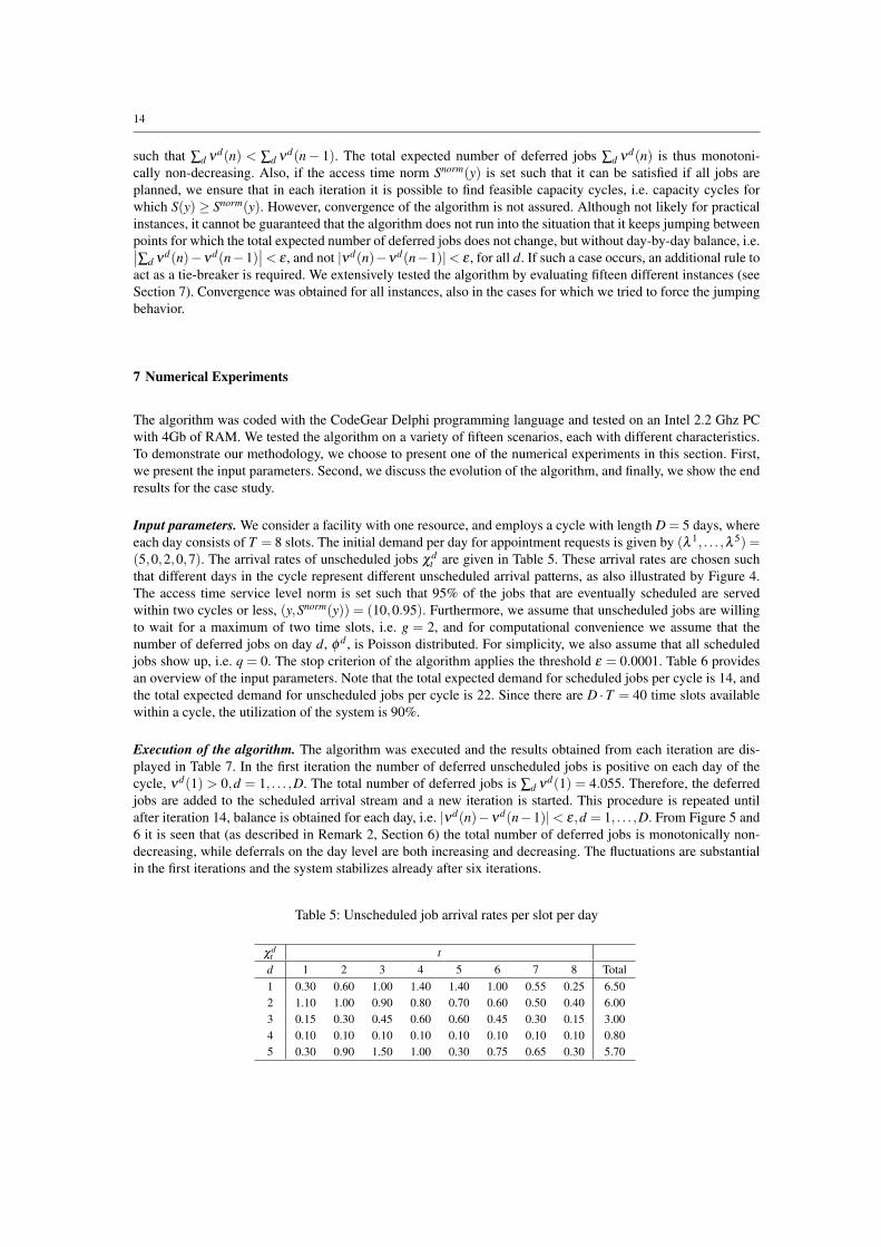
Input parameters. We consider a facility with one resource, and employs a cycle with length D = 5 days, where

each day consists of T = 8 slots. The initial demand per day for appointment requests is given by (λ 1, . . . ,λ 5) =(5,0,2,0,7). The arrival rates of unscheduled jobs χd

t are given in Table 5. These arrival rates are chosen such

that different days in the cycle represent different unscheduled arrival patterns, as also illustrated by Figure 4.

The access time service level norm is set such that 95% of the jobs that are eventually scheduled are served

within two cycles or less, (y,Snorm(y)) = (10,0.95). Furthermore, we assume that unscheduled jobs are willing

to wait for a maximum of two time slots, i.e. g = 2, and for computational convenience we assume that the

number of deferred jobs on day d, φ d , is Poisson distributed. For simplicity, we also assume that all scheduled

jobs show up, i.e. q = 0. The stop criterion of the algorithm applies the threshold ε = 0.0001. Table 6 provides

an overview of the input parameters. Note that the total expected demand for scheduled jobs per cycle is 14, and

the total expected demand for unscheduled jobs per cycle is 22. Since there are D ·T = 40 time slots available

within a cycle, the utilization of the system is 90%.

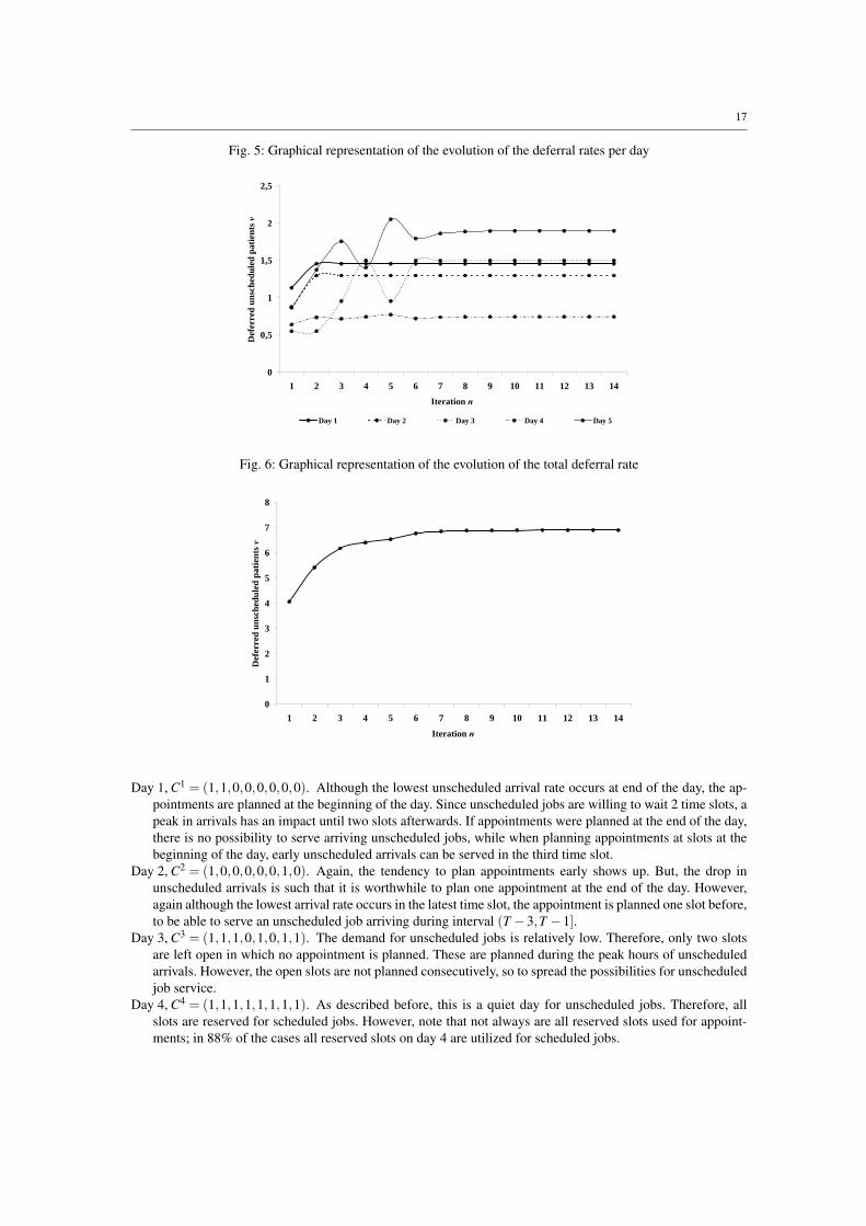
Execution of the algorithm. The algorithm was executed and the results obtained from each iteration are dis-

played in Table 7. In the first iteration the number of deferred unscheduled jobs is positive on each day of the

cycle, νd(1) > 0,d = 1, . . . ,D. The total number of deferred jobs is ∑d νd(1) = 4.055. Therefore, the deferred

jobs are added to the scheduled arrival stream and a new iteration is started. This procedure is repeated until

after iteration 14, balance is obtained for each day, i.e. |νd(n)−νd(n−1)|< ε,d = 1, . . . ,D. From Figure 5 and

6 it is seen that (as described in Remark 2, Section 6) the total number of deferred jobs is monotonically non-

decreasing, while deferrals on the day level are both increasing and decreasing. The fluctuations are substantial

in the first iterations and the system stabilizes already after six iterations.

Table 5: Unscheduled job arrival rates per slot per day

χdt t

d 1 2 3 4 5 6 7 8 Total

1 0.30 0.60 1.00 1.40 1.40 1.00 0.55 0.25 6.50

2 1.10 1.00 0.90 0.80 0.70 0.60 0.50 0.40 6.00

3 0.15 0.30 0.45 0.60 0.60 0.45 0.30 0.15 3.00

4 0.10 0.10 0.10 0.10 0.10 0.10 0.10 0.10 0.80

5 0.30 0.90 1.50 1.00 0.30 0.75 0.65 0.30 5.70

15

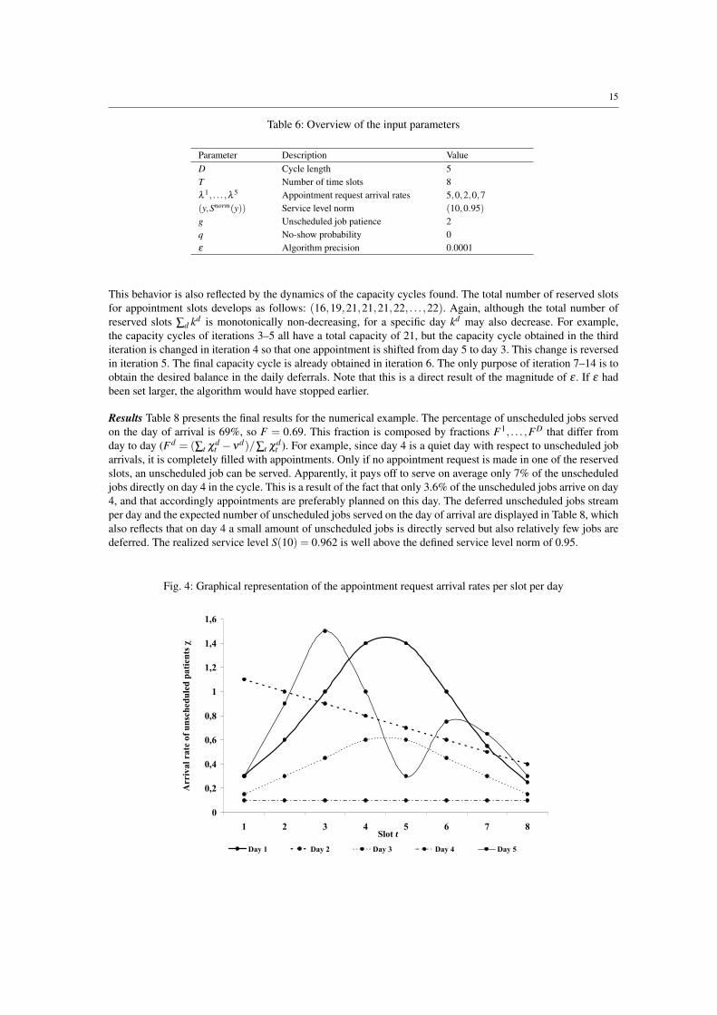
Table 6: Overview of the input parameters

Parameter Description Value

D Cycle length 5

T Number of time slots 8

λ 1, . . . ,λ 5 Appointment request arrival rates 5,0,2,0,7

(y,Snorm(y)) Service level norm (10,0.95)

g Unscheduled job patience 2

q No-show probability 0

ε Algorithm precision 0.0001

This behavior is also reflected by the dynamics of the capacity cycles found. The total number of reserved slots

for appointment slots develops as follows: (16,19,21,21,21,22, . . . ,22). Again, although the total number of

reserved slots ∑d kd is monotonically non-decreasing, for a specific day kd may also decrease. For example,

the capacity cycles of iterations 3–5 all have a total capacity of 21, but the capacity cycle obtained in the third

iteration is changed in iteration 4 so that one appointment is shifted from day 5 to day 3. This change is reversed

in iteration 5. The final capacity cycle is already obtained in iteration 6. The only purpose of iteration 7–14 is to

obtain the desired balance in the daily deferrals. Note that this is a direct result of the magnitude of ε . If ε had

been set larger, the algorithm would have stopped earlier.

Results Table 8 presents the final results for the numerical example. The percentage of unscheduled jobs served

on the day of arrival is 69%, so F = 0.69. This fraction is composed by fractions F1, . . . ,FD that differ from

day to day (Fd = (∑t χdt −νd)/∑t χd

t ). For example, since day 4 is a quiet day with respect to unscheduled job

arrivals, it is completely filled with appointments. Only if no appointment request is made in one of the reserved

slots, an unscheduled job can be served. Apparently, it pays off to serve on average only 7% of the unscheduled

jobs directly on day 4 in the cycle. This is a result of the fact that only 3.6% of the unscheduled jobs arrive on day

4, and that accordingly appointments are preferably planned on this day. The deferred unscheduled jobs stream

per day and the expected number of unscheduled jobs served on the day of arrival are displayed in Table 8, which

also reflects that on day 4 a small amount of unscheduled jobs is directly served but also relatively few jobs are

deferred. The realized service level S(10) = 0.962 is well above the defined service level norm of 0.95.

Fig. 4: Graphical representation of the appointment request arrival rates per slot per day

0

0,2

0,4

0,6

0,8

1

1,2

1,4

1,6

1 2 3 4 5 6 7 8Slot t

Arriv

al

ra

te o

f u

nsc

hed

ule

d p

ati

en

ts Ȥ

Day 1 Day 2 Day 3 Day 4 Day 5

16

Table 7: Results per iteration step of the algorithm

Iteration Day Tot. app. req. rate Deferral rate Difference Capacity cycle CAS

n d γd νd(n−1) νd(n) |νd(n−1)−νd(n−1)| kd Cd

1 1 5 0 1.133 1.133 1 (1,0,0,0,0,0,0,0)

2 0 0 0.865 0.865 1 (1,0,0,0,0,0,0,0)

3 2 0 0.547 0.547 4 (1,1,0,1,0,0,1,0)

4 0 0 0.637 0.637 8 (1,1,1,1,1,1,1,1)

5 7 0 0.873 0.873 2 (1,1,0,0,0,0,0,0)

2 1 6.133 1.133 1.456 0.323 2 (1,1,0,0,0,0,0,0)

2 0.865 0.865 1.296 0.431 2 (1,0,0,0,0,0,1,0)

3 2.547 0.547 0.549 0.002 4 (1,1,0,1,0,0,1,0)

4 0.637 0.637 0.736 0.099 8 (1,1,1,1,1,1,1,1)

5 7.873 0.873 1.371 0.498 3 (1,1,0,0,0,0,1,0)

3 1 6.456 1.456 1.456 0.000 2 (1,1,0,0,0,0,0,0)

2 1.296 1.296 1.296 0.000 2 (1,0,0,0,0,0,1,0)

3 2.549 0.549 0.952 0.403 5 (1,1,1,0,0,1,0,1)

4 0.736 0.736 0.715 0.021 8 (1,1,1,1,1,1,1,1)

5 8.371 1.371 1.752 0.381 4 (1,1,0,0,0,1,1,0)

4 1 6.456 1.456 1.456 0.000 2 (1,1,0,0,0,0,0,0)

2 1.296 1.296 1.296 0.000 2 (1,0,0,0,0,0,1,0)

3 2.952 0.952 1.498 0.546 6 (1,1,1,0,1,0,1,1)

4 0.715 0.715 0.742 0.027 8 (1,1,1,1,1,1,1,1)

5 8.752 1.752 1.402 0.350 3 (1,1,0,0,0,0,1,0)

5 1 6.456 1.456 1.456 0.000 2 (1,1,0,0,0,0,0,0)

2 1.296 1.296 1.296 0.000 2 (1,0,0,0,0,0,1,0)

3 3.498 1.498 0.954 0.544 5 (1,1,1,0,0,1,0,1)

4 0.742 0.742 0.771 0.029 8 (1,1,1,1,1,1,1,1)

5 8.402 1.402 2.049 0.647 4 (1,1,0,0,1,0,1,0)

6 1 6.456 1.456 1.456 0.000 2 (1,1,0,0,0,0,0,0)

2 1.296 1.296 1.296 0.000 2 (1,0,0,0,0,0,1,0)

3 2.954 0.954 1.495 0.541 6 (1,1,1,0,1,0,1,1)

4 0.771 0.771 0.721 0.050 8 (1,1,1,1,1,1,1,1)

5 9.049 2.049 1.794 0.255 4 (1,1,0,0,0,1,1,0)

.

.

....

14 1 6.456 1.456 1.456 0.000 2 (1,1,0,0,0,0,0,0)

2 1.296 1.296 1.296 0.000 2 (1,0,0,0,0,0,1,0)

3 3.497 1.497 1.497 0.000 6 (1,1,1,0,1,0,1,1)

4 0.743 0.743 0.743 0.000 8 (1,1,1,1,1,1,1,1)

5 8.897 1.897 1.897 0.000 4 (1,1,0,0,0,1,1,0)

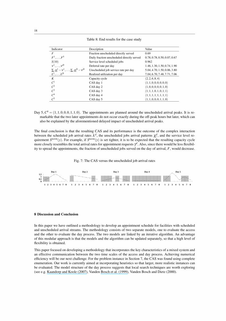
The resulting capacity cycle is K = (2,2,6,8,4), with corresponding day schedules which we discuss one-by-one

below. Note that to achieve the service level norm it is required to reserve a buffer capacity of 1.11 to account

for variability in appointment request arrivals, since 22 appointment slots are reserved while the average total

number of jobs to schedule within a cycle is ∑d(λd + νd) = 14+ 6.89 = 20.89. Apparently, the service level

norm is achieved with only 5% buffer capacity, thus reserved capacity for appointments can be used efficiently.

The realized expected load per day, denoted by L1, . . . ,LD, is a result of the capacity cycle, the probabilities that

the reserved appointment slots are utilized by appointment requests and the expected number of unscheduled

jobs served on day of arrival ∑t χdt −νd . It turns out that the load is balanced throughout the cycle where each

day has a realized load between 6.7 and 7.7.

Finally, we discuss the resulting day schedules, to explain the moments on which the appointments are planned

(see also Figure 7).

17

Fig. 5: Graphical representation of the evolution of the deferral rates per day

0

0,5

1

1,5

2

2,5

1 2 3 4 5 6 7 8 9 10 11 12 13 14

Iteration n

Def

erre

d un

sche

dule

d pa

tien

ts Ȟ

Day 1 Day 2 Day 3 Day 4 Day 5

Fig. 6: Graphical representation of the evolution of the total deferral rate

0

1

2

3

4

5

6

7

8

1 2 3 4 5 6 7 8 9 10 11 12 13 14

Iteration n

Def

erre

d un

sche

dule

d pa

tien

ts Ȟ

Day 1, C1 = (1,1,0,0,0,0,0,0). Although the lowest unscheduled arrival rate occurs at end of the day, the ap-

pointments are planned at the beginning of the day. Since unscheduled jobs are willing to wait 2 time slots, a

peak in arrivals has an impact until two slots afterwards. If appointments were planned at the end of the day,

there is no possibility to serve arriving unscheduled jobs, while when planning appointments at slots at the

beginning of the day, early unscheduled arrivals can be served in the third time slot.

Day 2, C2 = (1,0,0,0,0,0,1,0). Again, the tendency to plan appointments early shows up. But, the drop in

unscheduled arrivals is such that it is worthwhile to plan one appointment at the end of the day. However,

again although the lowest arrival rate occurs in the latest time slot, the appointment is planned one slot before,

to be able to serve an unscheduled job arriving during interval (T −3,T −1].Day 3, C3 = (1,1,1,0,1,0,1,1). The demand for unscheduled jobs is relatively low. Therefore, only two slots

are left open in which no appointment is planned. These are planned during the peak hours of unscheduled

arrivals. However, the open slots are not planned consecutively, so to spread the possibilities for unscheduled

job service.

Day 4, C4 = (1,1,1,1,1,1,1,1). As described before, this is a quiet day for unscheduled jobs. Therefore, all

slots are reserved for scheduled jobs. However, note that not always are all reserved slots used for appoint-

ments; in 88% of the cases all reserved slots on day 4 are utilized for scheduled jobs.

18

Table 8: End results for the case study

Indicator Description Value

F Fraction unscheduled directly served 0.69

F1, . . . ,F5 Daily fraction unscheduled directly served 0.78,0.78,0.50,0.07,0.67

S(10) Service level scheduled jobs 0.962

ν1, . . . ,νD Deferral rate per day 1.46,1.30,1.50,0.74,1.90

∑t χ1t −ν1, . . . ,∑t χD

t −νD Unscheduled job service rate per day 5.04,4.70,1.50,0.06,3.80

L1, . . . ,LD Realized utilization per day 7.04,6.70,7.48,7.71,7.06

K Capacity cycle (2,2,6,8,4)

C1 CAS day 1 (1,1,0,0,0,0,0,0)

C2 CAS day 2 (1,0,0,0,0,0,1,0)

C3 CAS day 3 (1,1,1,0,1,0,1,1)

C4 CAS day 4 (1,1,1,1,1,1,1,1)

C5 CAS day 5 (1,1,0,0,0,1,1,0)

Day 5, C4 = (1,1,0,0,0,1,1,0). The appointments are planned around the unscheduled arrival peaks. It is re-

markable that the two later appointments do not occur exactly during the off-peak hours but later, which can

also be explained by the aforementioned delayed impact of unscheduled arrival peaks.

The final conclusion is that the resulting CAS and its performance is the outcome of the complex interaction

between the scheduled job arrival rates λ d , the unscheduled jobs arrival patterns χdt , and the service level re-

quirement Snorm(y). For example, if Snorm(y) is set tighter, it is to be expected that the resulting capacity cycle

more closely resembles the total arrival rates for appointment requests γd . Also, since there would be less flexibil-

ity to spread the appointments, the fraction of unscheduled jobs served on the day of arrival, F , would decrease.

Fig. 7: The CAS versus the unscheduled job arrival rates

Day 2

1 2 3 4 5 6 7 8

Day 3

1 2 3 4 5 6 7 8

Day 1

00,5

11,5

1 2 3 4 5 6 7 8

Day 4

1 2 3 4 5 6 7 8

Day 5

1 2 3 4 5 6 7 8

8 Discussion and Conclusion

In this paper we have outlined a methodology to develop an appointment schedule for facilities with scheduled

and unscheduled arrival streams. The methodology consists of two separate models, one to evaluate the access

and the other to evaluate the day process. The two models are linked by an iterative algorithm. An advantage

of this modular approach is that the models and the algorithm can be updated separately, so that a high level of

flexibility is obtained.

This paper focused on developing a methodology that incorporates the key characteristics of a mixed system and

an effective communication between the two time scales of the access and day process. Achieving numerical

efficiency will be our next challenge. For the problem instance in Section 7, the CAS was found using complete

enumeration. Our work is currently aimed at incorporating heuristics so that larger, more realistic instances can

be evaluated. The model structure of the day process suggests that local search techniques are worth exploring

(see e.g. Kaandorp and Koole (2007), Vanden Bosch et al. (1999), Vanden Bosch and Dietz (2000).

19

Some extensions can readily be incorporated in our approach. Management is free to choose the service level

norm for the access time. As such, the resulting appointment schedules can be compared for several service lev-

els. Also, different choices for the time jobs are willing to wait (‘job patience’) could be studied or overbooking

to anticipate for no-shows. Furthermore, the access time for scheduled jobs and the fraction of unscheduled jobs

who cannot be served on the day of arrival are outcomes of model I and model II respectively, and serve as input

for the algorithm. Of course, other model outcomes could be chosen as well. Finally, to incorporate for example

planned maintenance of a service facility, the number of available slots in the day process can easily be amended

by closing slots. Worthwhile to consider would also be to introduce stochastic service times and job patience in

the day process. This might be a better reflection of reality, in particular in health care applications. Last but not

least, our focus will be on practical issues in the implementation of the methodology in health care settings in

Leiden University Medical Center and Academic Medical Center Amsterdam.

Acknowledgment 1 This research is supported by the Dutch Technology Foundation STW, applied sci-

ence division of NWO and the Technology Program of the Ministry of Economic Affairs.

Acknowledgment 2 The authors are grateful to the health care managers and medical doctors of Aca-

demic Medical Center Amsterdam and Leiden University Medical Center, who inspired us to take up this

research topic, the many fruitful discussions and their involvement in further development and implementation

of the methodology.

References

Adan, I., J.S.H. Van Leeuwaarden, E.M.M. Winands. 2006. On the application of Rouche’s theorem in queueing theory. Operations

Research Letters 34(3) 355–360.

Ashton, R., L. Hague, M. Brandreth, D. Worthington, S. Cropper. 2004. A simulation-based study of a NHS Walk-in Centre. Journal

of the Operational Research Society 56(2) 153–161.

Bruneel, H. 1993. Performance of discrete-time queueing systems. Computers & Operations Research 20(3) 303–320.

Bruneel, H., I. Wuyts. 1994. Analysis of discrete-time multiserver queueing models with constant service times. Operations Research

Letters 15(5) 231–236.

Cayirli, T., E. Veral. 2003. Outpatient scheduling in health care: a review of literature. Production and Operations Management 12(4)

519–549.

Cayirli, T., E. Veral, H. Rosen. 2006. Designing appointment scheduling systems for ambulatory care services. Health Care Manage-

ment Science 9(1) 47–58.

Cayirli, T., E. Veral, H. Rosen. 2008. Assessment of patient classification in appointment system design. Production and Operations

Management 17(3) 338–353.

Cochran, J.K., K.T. Roche. 2009. A multi-class queuing network analysis methodology for improving hospital emergency department

performance. Computers & Operations Research 36(5) 1497–1512.

Creemers, S. 2009. Appointment-Driven Queueing Systems. Ph.D. thesis, Katholieke Universiteit Leuven.

Creemers, S., M. Lambrecht. 2010. Queueing models for appointment-driven systems. Annals of Operations Research 178(1) 155–

172.

Dobson, G., S. Hasija, E.J. Pinker. 2011. Reserving capacity for urgent patients in primary care. Production and Operations Man-

agement 20(3) 456–473.

Goddard, J., M. Tavakoli. 2008. Efficiency and welfare implications of managed public sector hospital waiting lists. European Journal

of Operational Research 184(2) 778–792.

Green, L.V., P.J. Kolesar, J. Soares. 2001. Improving the SIPP approach for staffing service systems that have cyclic demands.

Operations Research 49(4) 549–564.

Green, L.V., S. Savin, B. Wang. 2006a. Managing patient service in a diagnostic medical facility. Operations Research 54(1) 11–25.

Green, L.V., J. Soares. 2007. Computing time-dependent waiting time probabilities in M(t)/M/s(t) queueing systems. Manufacturing

& Service Operations Management 9(1) 54–61.

Green, L.V., J. Soares, J.F. Giglio, R.A. Green. 2006b. Using queueing theory to increase the effectiveness of emergency department

provider staffing. Academic Emergency Medicine 13(1) 61–68.

Gupta, D., B. Denton. 2008. Appointment scheduling in health care: Challenges and opportunities. IIE Transactions 40(9) 800–819.

Hassin, R., S. Mendel. 2008. Scheduling arrivals to queues: A single-server model with no-shows. Management Science 54(3)

565–572.

20

Ho, C.J., H.S. Lau. 1992. Minimizing total cost in scheduling outpatient appointments. Management Science 38(12) 1750–1764.

Kaandorp, G.C., G. Koole. 2007. Optimal outpatient appointment scheduling. Health Care Management Science 10(3) 217–229.

Klassen, K.J., T.R. Rohleder. 1996. Scheduling outpatient appointments in a dynamic environment. Journal of Operations Manage-

ment 14(2) 83–101.

Klassen, K.J., T.R. Rohleder. 2004. Outpatient appointment scheduling with urgent clients in a dynamic, multi-period environment.

International Journal of Service Industry Management 15(2) 167–186.

Kleinrock, L. 1975. Queueing systems, volume 1: theory. John Wiley & Sons, London, UK.

Kolisch, R., S. Sickinger. 2008. Providing radiology health care services to stochastic demand of different customer classes. OR

Spectrum 30(2) 375–395.

Kopach, R., P.C. DeLaurentis, M. Lawley, K. Muthuraman, L. Ozsen, R. Rardin, H. Wan, P. Intrevado, X. Qu, D. Willis. 2007. Effects

of clinical characteristics on successful open access scheduling. Health Care Management Science 10(2) 111–124.

LaGanga, L.R., S.R. Lawrence. 2007. Clinic overbooking to improve patient access and increase provider productivity*. Decision

Sciences 38(2) 251–276.

Lehaney, B., S.A. Clarke, R.J. Paul. 1999. A case of an intervention in an outpatients department. Journal of the Operational Research

Society 50(9) 877–891.

Liao, C.J., C.D. Pegden, M. Rosenshine. 1993. Planning timely arrivals to a stochastic production or service system. IIE Transactions

25(5) 63–73.

Liu, L., X. Liu. 1998. Dynamic and static job allocation for multi-server systems. IIE Transactions 30(9) 845–854.

Liu, N., S. Ziya, V.G. Kulkarni. 2010. Dynamic scheduling of outpatient appointments under patient no-shows and cancellations.

Manufacturing & Service Operations Management 12(2) 347–364.

Murray, M., D.M. Berwick. 2003. Advanced access: reducing waiting and delays in primary care. Journal of the American Medical

Association 289(8) 1035–1040.

Patrick, J., ML Puterman. 2007. Improving resource utilization for diagnostic services through flexible inpatient scheduling: A method

for improving resource utilization. Journal of the Operational Research Society 58(2) 235–245.

Patrick, J., M.L. Puterman, M. Queyranne. 2008. Dynamic multi-priority patient scheduling for a diagnostic resource. Operations

Research 56(6) 1507–1525.

Pegden, C.D., M. Rosenshine. 1990. Scheduling arrivals to queues. Computers & Operations Research 17(4) 343–348.

Qu, X., R.L. Rardin, J.A.S. Williams, D.R. Willis. 2007. Matching daily healthcare provider capacity to demand in advanced access

scheduling systems. European Journal of Operational Research 183(2) 812–826.

Qu, X., J. Shi. 2009. Effect of two-level provider capacities on the performance of open access clinics. Health Care Management

Science 12(1) 99–114.

Ramakrishnan, M., D. Sier, P.G. Taylor. 2005. A two-time-scale model for hospital patient flow. IMA Journal of Management

Mathematics 16(3) 197.

Reilly, T.A., V.P. Marathe, B.E. Fries. 1978. A delay-scheduling model for patients using a walk-in clinic. Journal of Medical Systems

2(4) 303–313.

Sickinger, S., R. Kolisch. 2009. The performance of a generalized Bailey–Welch rule for outpatient appointment scheduling under

inpatient and emergency demand. Health Care Management Science 12(4) 408–419.

Su, S., C.L. Shih. 2003. Managing a mixed-registration-type appointment system in outpatient clinics. International Journal of

Medical Informatics 70(1) 31–40.

Swisher, J.R., S.H. Jacobson, J.B. Jun, O. Balci. 2001. Modeling and analyzing a physician clinic environment using discrete-event

(visual) simulation. Computers & Operations Research 28(2) 105–125.

Takagi, H. 1988. Queuing analysis of polling models. ACM Computing Surveys (CSUR) 20(1) 5–28.

Vanden Bosch, P.M.V., D.C. Dietz. 2000. Minimizing expected waiting in a medical appointment system. IIE Transactions 32(9)

841–848.

Vanden Bosch, P.M.V., D.C. Dietz, J.R. Simeoni. 1999. Scheduling customer arrivals to a stochastic service system. Naval Research

Logistics 46(5) 549–559.

Wang, P.P. 1999. Sequencing and scheduling N customers for a stochastic server. European Journal of Operational Research 119(3)

729–738.

Williams, P., G. Tai, Y. Lei. 2010. Simulation based analysis of patient arrival to health care systems and evaluation of an operations

improvement scheme. Annals of Operations Research 1–17.

Worthington, DJ. 1987. Queueing models for hospital waiting lists. Journal of the Operational Research Society 38(5) 413–422.