Detached eddy simulation of turbulent flow and heat transfer in a two-pass internal cooling duct

Detached Eddy Simulation of Turbulent Flow and Heat Transfer in Turbine Blade Internal Cooling Ducts

Aroon K Viswanathan

Dissertation submitted to the faculty of Virginia Polytechnic Institute and State University in partial fulfillment of the requirements for the degree of

Doctor of Philosophy in

Mechanical Engineering

Dr. Danesh K. Tafti, Chair Dr. William J. Devenport

Dr. Thomas E. Diller Dr. Muhammad R. Hajj

Dr. Wing F. Ng

July 31, 2006 Blacksburg, Virginia

Keywords: Detached Eddy Simulations (DES), Coriolis forces, centrifugal buoyancy, ribbed ducts, turbine blade internal cooling

Detached Eddy Simulation of Turbulent Flow and Heat Transfer in Turbine Blade Internal Cooling Ducts

Aroon K Viswanathan

Abstract Detached Eddy Simulations (DES) is a hybrid URANS-LES technique that was

proposed to obtain computationally feasible solutions of high Reynolds number flows undergoing massive separation with reliable accuracy. Since its inception, DES has been applied to a wide variety of flow fields, but mostly limited to unbounded external aerodynamic flows. This is the first study to apply and validate DES to predict the internal flow and heat transfer in non-canonical flows of industrial relevance. The prediction capabilities of DES in capturing the effects of Coriolis forces, which are induced by rotation, and centrifugal buoyancy forces, which are induced by thermal gradients, are also authenticated.

The accurate prediction of turbulent flows is sensitive to the level of turbulence predicted by the turbulence scheme. By treating the regions of interest in LES mode, DES allows the unsteadiness in these regions to develop and hence predicts the turbulence levels accurately. Additionally, this permits DES to capture the effects of system rotation and buoyancy. Computations on a rotating system (a sudden expansion duct) and a system subjected to thermal gradients (cavity with a heated wall) validate the prediction capability of DES.

The application of DES is further extended to a non-canonical, internal flow which is of relevance in internal cooling of gas turbine blades. Computations of the fully developed flow and heat transfer shows that DES surpasses several shortcomings of the RANS model on which it is based. DES accurately predicts the primary and secondary flow features, the turbulence characteristics and the heat transfer in stationary ducts and in rotating ducts, where the effects of Coriolis forces and centrifugal buoyancy forces are dominant. DES computations are carried out at a computational cost that is almost an order of magnitude less than the LES with little compromise on the accuracy.

However, the capabilities of DES in predicting the transition to turbulence are inadequate, as highlighted by the flow features and the heat transfer in the developing region of the duct. But once the flow becomes fully turbulent, DES predicts the flow physics and shows good quantitative agreement with the experiments and LES.

iii

Granting Institution

This research was supported by the US DOE, Office of Fossil Energy, and National

Energy Technology Laboratory. Any opinions, findings, conclusions, or recommendations

expressed herein are those of the authors and do not necessarily reflect the views of the

DOE.

iv

To my parents, mentors and friends

v

Acknowledgements Working on this dissertation over the last three years has been pretty rewarding in

terms of the knowledge and insight I have gained in the field of turbulence modeling. In the course of this I have got advice, help and encouragement from many people whom I would like to thank. I am extremely grateful for the guidance of my advisor, Dr. Danesh Tafti. His mentoring, encouragement and optimism have consistently helped me get over the several obstacles that I have run into during this period. He has always been present in his office and the lab, even during off-hours like semester breaks, weekends and late evenings, to answer my queries. His code GenIDLEST has been used for running all the calculations presented in this dissertation.

I would also like to thank my committee members Dr. Devenport, Dr. Diller, Dr. Hajj and Dr. Ng for reviewing my work and providing valuable suggestions during my preliminary defense.

I have been privileged to work with my colleagues at the HPCFD lab. I would like to thank Evan Sewall, Samer Abdel-Wahab, Wilfred Patrick and Sundar Narayan from whom I learnt a lot during the first year of my PhD. Special thanks to Emily Sewall for the snacks and cookies which she used to send with Evan. I would also like to thank the other members of the HPCFD lab: Ali Rozati, Shi Ming Li, Ju Kim, Anant Shah, Mohammad Elyyan, Pradeep Gopalakrishnan and Keegan Delaney with whom learnt and shared a good deal of knowledge. Ali, Mohammad, I’ll keep checking the ESPN web-page for updates on the NBA 2007 draft. Hope to see you guys in the first round of the draft.

I have enjoyed the company of my dearest friends Giridhar, Kavita, Ashvin, Vikram, Wilfred and Leepika. Thank you for being with me during thick and thin. Thank you Giridhar for your company during our regular weekend hikes. I wouldn’t have explored Blacksburg as much without you. Thank you Kavita for your constant (and loud) lectures on how CLA and PPAR- affect the fat content in my body. I know for sure that these have had a severe effect on my hearing. I have also had the privileged company of several others – Nitin, Owais, Umesh, Pratik, Ritesh and Akhilesh who have hung out with me during the past three years.

I would also like to thank Dr. Don Waldron and Dr. (Mrs.) Claire Waldron, who were my hosts in Blacksburg. They were my family away from home and took care of me during the three years.

Finally, I owe the most to my parents who have encouraged me all through me graduate studies. To them, to my mentors and to my friends, I dedicate this work.

vi

Project Description

This study is a subset of the project “Enhanced Prediction Techniques Based on Time-

Accurate Simulations for Turbine Blade Internal Cooling” which aims at applying,

developing and demonstrating the use of high-fidelity Large Eddy Simulations (LES) and

a hybrid RANS-LES technique – Detached Eddy Simulations (DES) as accurate

prediction tools for the analysis of the three-dimensional, unsteady flow and heat transfer

in rotating internal cooling ducts. These computational approaches are integrated with

experiments from the literature and three-component mean and turbulent flow field

measurements made in a large scale ribbed channel using Laser Doppler Velocimetry

(LDV).

The project studies the application of the computational techniques in internal cooling

geometries with ribs. Of prime interest are: (a) the developing flow regime (b) the fully

developed region, and (c) the 180º bend region that connects two passes of the cooling

duct. LES has been applied in the fully developed region for stationary internal cooling

ducts by D. K. Tafti and in rotating ducts by Samer Abdel-Wahab. More recent work on

the application of LES to the developing region and the 180º bend of the duct for

stationary ducts as well as rotating ducts, where the flow is affected by Coriolis forces

and centrifugal buoyancy was carried out by Evan Sewall.

The application of DES in these studies is aimed at cutting down the cost of the

computation as compared to LES while not compromising on the accuracy. The

performance of DES is initially evaluated in the fully developed region of the ribbed

duct. The performance of DES in predicting the flow and heat transfer in stationary and

rotating ducts is validated from experiments in literature and earlier LES calculations.

vii

Since DES is computationally less intensive than LES, it is feasible to study a complete

two-pass duct which combines all the cases individually studied by LES – the developing

region of the flow, the fully developed region and the 180º bend. These studies are

validated with experiments from literature, experiments as a part of this project (assisted

by K. A. Thole) and the LES computations.

As of date, 15 conference papers and 8 journal papers have been published from this

project. From the DES computations, which were carried out with the assistance of D. K.

Tafti, 2 conference papers and 4 journal papers have been published. A list of all the

publications is shown in Table 1. The relevant publications have been highlighted in the

Table and the abstracts of these publications are reproduced in Appendix C.

Table 1: List of publications from the project "Enhanced Prediction Techniques Based on Time-Accurate Simulations for Turbine Blade Internal Cooling"

Paper Publication Year

Tafti D. K., Large Eddy Simulations of Heat Transfer in A Ribbed Channel for Internal Cooling of Turbine Blades, Paper No. GT2003-38122, Proceedings of ASME/IGTI Turbo Expo., Atlanta, Georgia, June 16-19, 2003.

2003

Tafti, D. K., Evaluating the Role of Subgrid Stress Modeling in a Ribbed Duct for the Internal Cooling of Turbine Blades, Int. J. Heat Fluid Flow, 26, pp 92-104, 2005

2005

Abdel-Wahab, S. and Tafti, D. K., Large Eddy Simulation of Flow and Heat Transfer in a Staggered 45o Ribbed Duct, GT2004-53800, ASME Turbo Expo: 2004, Vienna, Austria.

2004

Abdel-Wahab, S. and Tafti, D. K., Large Eddy Simulations of Flow and Heat Transfer in a 90o Ribbed Duct with Rotation - Effect of Coriolis Forces, GT2004-53796, ASME Turbo Expo: 2004, Vienna, Austria.

2004

Abdel-Wahab, S. and Tafti, D. K., Large Eddy Simulations of Flow and Heat Transfer in a 90o Ribbed Duct with Rotation - Effect of Buoyancy Forces, GT2004-53799, ASME Turbo Expo: 2004, Vienna, Austria.

2004

Abdel-Wahab, S. and Tafti, D. K., Large Eddy Simulations of Flow and Heat Transfer in a 90º Ribbed Duct with Rotation - Effect of Coriolis and Centrifugal Buoyancy Forces, J. Turbomachinery, 126, pp 627-636, 2005.

2005

viii

Sewall, E, and Tafti, D. K., Large Eddy Simulation of the Developing Region of a Stationary Ribbed Internal Turbine Blade Cooling Channel, GT2004-53832, ASME Turbo Expo: 2004, Vienna, Austria

2004

Sewall, E, and Tafti, D. K., Large Eddy Simulation of the Developing Region of a Rotating Ribbed Internal Turbine Blade Cooling Channel, GT2004-53833, ASME Turbo Expo: 2004, Vienna, Austria.

2004

Graham, A., Sewall, E., Thole, K.A., Flowfield Measurements in a Ribbed Channel Relevant to Internal Turbine Blade Cooling, GT2004-53361, ASME Turbo Expo: 2004, Vienna, Austria.

2004

Sewall, E, and Tafti, D. K., Large Eddy Simulation of Flow and Heat Transfer in the Developing Flow Region of a Rotating Gas Turbine Blade Internal Cooling Duct with Coriolis and Buoyancy Forces, GT2005-68519, ASME Turbo Expo, Reno-Tahoe, USA

2005

Sewall, E, and Tafti, D. K., Large Eddy Simulation of Flow and Heat Transfer in the 180 Degree Bend Region of a Stationary Ribbed Gas Turbine Blade Internal Cooling Duct, GT2005-68518, ASME Turbo Expo, Reno-Tahoe, USA

2005

Sewall, E, and Tafti, D. K., Large Eddy Simulation of Flow and Heat Transfer in the 180 Degree Bend Region of a Stationary Ribbed Gas Turbine Blade Internal Cooling Duct, In press ASME J. Turbomachinery.

2005

Sewall, E.A., Tafti, D.K., Graham, A.B., Thole, K.A., Experimental Validation of Large Eddy Simulations of Flow and Heat Transfer in a Stationary Ribbed Duct, , Int. J. Heat Fluid Flow, 27, pp 243-258, 2006

2006

Viswanathan, A.K., Tafti, D.K., “Detached Eddy Simulation of Turbulent Flow and Heat Transfer in a Ribbed Duct”, HT-FED04-56152, Proceedings of Heat Transfer/ Fluids Engineering Summer Conference ASME, July 11-15, Charlotte, USA.

2004

Viswanathan, A.K., Tafti, D.K., Abdel-Wahab., S., “Large Eddy Simulation of Flow and Heat Transfer in an Internal Cooling Duct with High Blockage Ratio 45° Staggered Ribs”, GT2005-68086, ASME Turbo Expo 2005, June 6-9, Reno-Tahoe, USA.

2005

Viswanathan, A.K., Tafti, D.K., “Large Eddy Simulation in a Duct with Rounded Skewed Ribs”, GT2005-68117, ASME Turbo Expo 2005, June 6-9, Reno-Tahoe, USA.

2005

ix

Viswanathan, A.K., Tafti, D.K., “Detached Eddy Simulation of Flow and Heat Transfer in a Stationary Internal Cooling Duct with Skewed Ribs”, GT2005-68118, ASME Turbo Expo 2005, June 6-9, Reno-Tahoe, USA.

2005

Viswanathan, A.K., Tafti, D.K., “Detached Eddy Simulation of Turbulent Flow and Heat Transfer in a Ribbed Duct”, ASME Journal of Fluids Engineering, 127(5), pp 888-896, September 2005

2005+

Viswanathan, A.K., Tafti, D.K., “A Comparative Study of DES and URANS in a Two-pass Internal Cooling Duct with Normal Ribs”, IMECE2005-79288, ASME International Mechanical Engineering Congress and Exposition 2005, November 5-11, Orlando, Florida, USA.

2005+

Viswanathan, A.K., Tafti, D.K., “Detached Eddy Simulation of Turbulent Flow and Heat Transfer in a Two-pass Internal Cooling Duct”, Int J of Heat and Fluid Flow, 27, pp 1 – 20, 2006.

2006*

Viswanathan, A.K., Tafti, D.K., “Large Eddy Simulation of the fully developed Flow and Heat Transfer in a Rotating Duct with 45° Ribs”, GT2006-90229, ASME Turbo Expo 2006, May 8-11, Barcelona, Spain.

2006

Viswanathan A.K., Tafti, D. K., 2005, Detached Eddy Simulation of Flow and Heat Transfer in Fully Developed Rotating Internal Cooling Channel with Normal Ribs , Int. J Heat and Fluid Flow. 27, pp 351-370, 2006

2006∗

Viswanathan, A.K., Tafti, D.K., “A Comparative Study of DES and URANS for Flow Prediction in a Two-pass Internal Cooling Duct”, In press ASME Journal of Fluids Engineering

2006

+ Figures and tables are reprinted with permission from ASME ∗ Figures are reprinted with permission from Elsevier

x

Table of contents

Abstract................................................................................................................. ii Project Description............................................................................................... vi List of Tables....................................................................................................... xii List of Figures .....................................................................................................xiii Nomenclature ..................................................................................................... xx 1 Introduction .....................................................................................................1

1.1 Problem Description...................................................................................5 2 Literature Review............................................................................................9

2.1 Stationary Internal Flows ..........................................................................10 2.2 Modeling the Effect of Coriolis Forces......................................................12 2.3 Modeling the Effect of Buoyancy Forces ..................................................15

3 Computational Model and Governing Equations...........................................22

3.1 Mean Flow and Energy Equations ...........................................................22 3.2 Turbulence Models...................................................................................23

3.2.1 k- Equations (1988 Wilcox Model)..................................................23 3.2.2 Menter’s Baseline Model...................................................................24 3.2.3 Shear-Stress Transport (SST) Model ................................................26

3.3 Detached Eddy Simulations .....................................................................26 3.4 Numerical Method ....................................................................................28 3.5 Post-processing .......................................................................................29

4 Validation Cases – Effects of Rotation and Buoyancy...................................31

4.1 Capturing the Effects of Rotation in Sudden Expansion Channels using Detached Eddy Simulations.............................................................................31

4.1.1 Computational Details .......................................................................33 4.1.2 Grid Sensitivity ..................................................................................34 4.1.3 Comparison of Turbulence Strategies ...............................................35 4.1.4 DES Regions ....................................................................................38 4.1.5 Flow Characteristics..........................................................................40 4.1.6 Conclusions ......................................................................................44

4.2 Prediction of the Turbulent Cavity Flow driven by Shear and Buoyancy using Detached Eddy Simulations ...................................................................45

4.2.1 Computational Details .......................................................................46 4.2.2 Effect of Grid Density ........................................................................48 4.2.3 Effect of additional buoyancy terms ..................................................49 4.2.4 Effects of buoyancy...........................................................................50 4.2.5 Conclusions ......................................................................................52

xi

5 Flow and Heat Transfer in the Fully Developed Ribbed Duct........................53

5.1 Grid Sensitivity Comparisons ...................................................................55 5.2 DES Regions............................................................................................57 5.3 Stationary Duct.........................................................................................59

5.3.1 Flow Field Predictions.......................................................................59 5.3.2 Heat Transfer Enhancement .............................................................64 5.3.3 Summary and Conclusions ...............................................................68

5.4 Rotating Duct - Effects of Coriolis Forces.................................................69 5.4.1 Mean Flow field.................................................................................70 5.4.2 Turbulent Flow Characteristics..........................................................75 5.4.3 Mean Heat Transfer ..........................................................................77 5.4.4 Conclusions ......................................................................................83

5.5 Rotating Ducts - Effects of Coriolis Forces and Centrifugal Buoyancy .....85 5.5.1 Effects of Centrifugal Buoyancy ........................................................86 5.5.2 Mean Flow Features .........................................................................87 5.5.3 Turbulent Flow Features ...................................................................91 5.5.4 Heat Transfer Augmentation .............................................................93 5.5.5 Summary and Conclusions .............................................................100

6 Flow and Heat Transfer in a complete Two Pass Duct connected by a 180º Bend .................................................................................................................103

6.1 Stationary Two-Pass Duct ......................................................................105 6.1.1 Mean Flow Field..............................................................................106 6.1.2 Summary and Conclusions .............................................................126

6.2 Rotating Two Pass Duct – Effect of Coriolis Forces ...............................128 6.2.1 Developing Flow .............................................................................129 6.2.2 Heat Transfer Augmentation in the First Pass.................................132 6.2.3 Flow in the 180º Bend .....................................................................135 6.2.4 Heat Transfer in the 180º Bend.......................................................137 6.2.5 Pitch Averaged Friction Factor ........................................................139 6.2.6 Rib Averaged Heat Transfer Augmentation .....................................142 6.2.7 Summary and Conclusions .............................................................143

7 Summary and Conclusions .........................................................................145

7.1 Recommendations .................................................................................145 References .......................................................................................................148 Appendix A: Additional Buoyancy Production Term in the k-equation ...............156 Appendix B: Dimensionless Parameters...........................................................158 Appendix C: Abstracts of relevant publications .................................................160

xii

List of Tables

Table 1: List of publications from the project "Enhanced Prediction Techniques Based on Time-Accurate Simulations for Turbine Blade Internal Cooling".......... vii Table 2: Variation in the coefficient of the buoyancy production term in the or equation used by different groups.......................................................................19 Table 3: Extra terms in the momentum (Su) and energy equations (S) for the different cases studied ........................................................................................23 Table 4: a-posteriori comparison of the grid dimensions in the three directions for the DES grids......................................................................................................55 Table 5 : Percentage form and friction drag in the ribbed duct ...........................59 Table 6 : Comparison of the overall friction factor. ..............................................63 Table 7 : Comparison of the overall heat transfer augmentation ........................67 Table 8: Variation of the heat transfer augmentation at the ribbed and side walls for different rotation and buoyancy cases .........................................................100 Table 9: Comparison of the surface pressure drop as predicted by the current computation in comparison with the experimental measurements by Prabhu and Vedula (2003) for the rotating duct....................................................................141

xiii

List of Figures

Figure 1: (a) The cross-section of the first stage rotating blade used in the Siemens - Westinghouse 501-F Engine (Courtesy: Howard, G., O'Brein, W.F.,) (b) Schematic diagram of the turbine balde cross-section (Han, J.C., 1988) showing the region of interest .............................................................................................6 Figure 2: Geometry used for computation of flow downstream of a back-facing step. The effect of clockwise (negative) rotation and anti-clockwise (positive) rotation are also shown. Red arrows show the effect of Coriolis forces on the reattachment. ......................................................................................................32 Figure 3: Grid distribution in the x, y, z directions downstream of the back-facing step, for the aspect ratio 2 channel. ....................................................................34 Figure 4: Comparison of the reattachment lengths for the three grids used for DES Computation ...............................................................................................35 Figure 5: Comparison of the reattachment lengths downstream of the back-facing step for a stationary case (Ro = 0.00, Aspect ratio = 2). LES = 5.25, DES = 7.20, URANS = 10.00 .........................................................................................36 Figure 6: Comparison of the reattachment lengths as predicted by DES k- (Duct AR = 2), URANS k- (AR = 2) and earlier studies by Nilsen and Andersson (1990) (Re = 5500, AR = 2) and Iaccarino et al., (1999) with experimental measurements by Rothe and Johnston (1979). ..................................................37 Figure 7: Instantaneous coherent vorticity contours downstream of the back-facing step (AR = 2), at the center of the duct for DES (Top) and URANS (Bottom). .............................................................................................................38 Figure 8: DES regions downstream of the back-facing step showing the dominance of LES characteristics in the region of separation (Case shown is Ro = 0.04).................................................................................................................39 Figure 9: Iso-surfaces of coherent vorticity to show the stabilizing (Ro = -0.08) and the destabilizing effects (Ro = 0.08) of rotation on the flow downstream of the backfacing step. (Aspect Ratio = 5) ....................................................................40 Figure 10: Variation of the reattachment lengths at the center of the channel with rotation number for the duct of aspect ratio 5 (Top) and 2 (Bottom)....................41 Figure 11: Comparison of the reattachment lengths for a duct of (a) AR = 5 (b) AR = 2.................................................................................................................43

xiv

Figure 12: Top view of the instantaneous coherent vortices downstream of a backward facing step for ducts of aspect ratio 2 (Top) and aspect ratio 5 (bottom)............................................................................................................................44 Figure 13: Schematic diagram of the 2D cavity studied. Periodic boundary conditions are used in the z direction..................................................................46 Figure 14: Schematic diagram showing the measurement planes where the temperature profiles have been reported ............................................................47 Figure 15: Grid independency study comparing the spatial variation of temperature predicted by DES and LES with experimental data. Data has been extracted at the vertical center (y/L = 0.5) and horizontal center (x/L = 0.5) of the cavity...................................................................................................................48 Figure 16: Effect of the buoyancy term in the URANS (Top) and DES (Bottom) calculation. Data has been extracted at the vertical center (y/L = 0.5) and horizontal center (x/L = 0.5) of the cavity ............................................................50 Figure 17: Effect of buoyancy in influencing the temperature in the cavity at y/L = 0.5 and at x/L = 0.5 .............................................................................................51 Figure 18: Comparison of the spatial variation of temperature (LES on 64 x 64 x 64 grid, DES and URANS on 32 x 32 x 32 grid) with experiments by Grand (1975), for a high buoyancy case........................................................................51 Figure 19 : The computational model - A pair of ribs placed at the center of the duct. Flow in the duct is periodic in the streamwise direction..............................54 Figure 20 : Comparison of the streamwise velocities in a plane through the ribs (y/e = 0.25) for the (a) 483 grid (b) 643 grid (c) 963 grid (d) LES 1283 case. 643 and the 963 case show the best agreement. 483 grid overpredits the extent of the recirculation region..............................................................................................56 Figure 21 : Plot of the LES and RANS region in the DES computation for the 643 grid in a Z plane. A value of 1 represents a complete LES region and a value of 0 a complete RANS region. Flow is periodic in the streamwise direction...............58 Figure 22 : Streamwise velocity distributions at the center of the duct at y/e = 0.1 in comparison with the experimental measurements by Rau et al., (1998) .........60 Figure 23 : Comparison of streamwise velocity distributions at y/e = 0.25 for the (a) k- DES case (b) SST DES case (c) k- RANS case (d) LES case.............61 Figure 24 : Comparison of the secondary flow distribution at y/e = 1.5 and z/Dh = 0.45.....................................................................................................................62

xv

Figure 25 : Comparison of the secondary flow (a) predicted by DES k- model (b) DES SST model (c) k- RANS model (d) Experimental (Liou et al.). ............63 Figure 26 : Streamlines showing the recirculation region in front of the rib and primary and secondary circulations behind the rib and their effect on heat transfer on the walls. Red regions represent high heat transfer, while blue regions represent low heat transfer. ................................................................................64 Figure 27 : Comparison of augmentation ratios on the ribbed floor for the (a) k- DES case (b) Menter's SST DES case (c) k- RANS case (d) LES case ..........65 Figure 28 : Comparison of the augmentation ratios (a) at the center of the ribbed floor (b) side walls upstream of the rib ................................................................66 Figure 29 : Comparison of the heat transfer augmentation ratios on the side walls (a) k- DES (b) Menter’s SST DES (c) k- RANS (d) LES .......................67 Figure 30: Effect of Coriolis forces in a square duct subjected to rotation..........69 Figure 31: Streamlines showing the flow in a fully developed duct as predicted by DES SST at Z = 0.5 (a) Ro = 0.18 (b) Ro = 0.35 (c) Ro = 0.67. Y = 0 represents the trailing wall, while Y = 1 represents the leading wall. Flow direction is from left to right.................................................................................................................71 Figure 32: Streamlines showing the flow in a fully developed duct rotating at Ro = 0.35 at Z = 0.5 as predicted by (a) LES (b) DES SST (c) URANS SST. Y = 0 represents the trailing wall, while Y = 1 represents the leading wall. Flow direction is from left to right. ..............................................................................................73 Figure 33: Secondary flow contours on the rib for (a) Ro = 0.0 (b) Ro = 0.18 (c) Ro = 0.35 (d) Ro = 0.67 as predicted by DES SST. The contours show the effect of rotation on the secondary flow in the cross-section. .......................................74 Figure 34: TKE values as predicted by the DES, LES and the URANS cases for the three rotation cases in between the ribs at z = 0.5........................................75 Figure 35: Coherent vorticity contours for the (a) LES 1283 (b) DES 643 (c) URANS 643 for Ro = 0.35 show the scales resolved of the three schemes. .......76 Figure 36: Heat transfer augmentation (Nu/Nu0) predicted at the leading and the trailing walls by DES SST for (a) Ro = 0.18 (b) Ro = 0.35 (c) Ro = 0.67. Flow direction is from left to right. ................................................................................77

xvi

Figure 37: Heat transfer augmentation (Nu/Nu0) predicted at the leading (upper half of the plot) and the trailing walls (lower half of the plot) for the Ro = 0.35 case by (a) LES (b) DES SST(c) URANS SST. Flow direction is from left to right.......78 Figure 38: Heat transfer augmentation (Nu/Nu0) predicted at the side wall by DES SST for the (a) Ro = 0.18 (b) Ro = 0.35 (c) Ro = 0.67. Flow direction is from left to right. ..........................................................................................................80 Figure 39: Heat transfer augmentation (Nu/Nu0) predicted at the side wall for the Ro = 0.35 case by (a) LES (b) DES SST(c) URANS SST. Flow direction is from left to right. ..........................................................................................................81 Figure 40: Side wall heat transfer predicted by LES, DES and URANS for the various rotation cases. ........................................................................................81 Figure 41: Comparison of average Nusselt number augmentation ratios at the leading and trailing sides with experiments.........................................................82 Figure 42: Effect of Coriolis forces (F) and Centrifugal Buoyancy (Fb) in rotating ducts ...................................................................................................................86 Figure 43: Comparison of the recirculation regions at the leading edge for the three rotation cases with Bo = 0.12.....................................................................88 Figure 44: Comparison of the recirculation regions at the leading edge for the three different buoyancy cases with Ro = 0.35. ..................................................89 Figure 45: Comparison of the secondary velocities for Ro = 0.35 for varying buoyancies (a) Bo = 0.00 (b) Bo = 0.12 (c) Bo = 0.29.........................................90 Figure 46: Comparison of the secondary flows as predicted by DES and LES at the center of the rib region for Bo = 0.29 and Ro = 0.35, for (a) DES (b) LES. ...91 Figure 47: Comparison of the turbulent kinetic energy in between two consecutive ribs at z = 0.5. .................................................................................92 Figure 48: Heat transfer distribution at the center of the duct (z/Dh =0.5) at the leading and trailing surfaces. Buoyancy in all the cases is Bo = 0.12 .................93 Figure 49: Heat transfer distribution at the ribbed walls for varying buoyancy numbers for a constant Ro = 0.35.......................................................................94 Figure 50: Effect of the variation of rotation and buoyancy on the heat transfer at the side walls, plotted at a distance of 0.5e upstream of the ribs. .......................96

xvii

Figure 51: Comparison of the ribbed (Top) and side wall (Bottom) heat transfer predicted by DES and LES for Ro = 0.35 and Bo = 0.29 ....................................97 Figure 52: Comparison of the surface averaged ribbed wall heat transfer augmentation ......................................................................................................99 Figure 53: Comparison of the side wall heat transfer augmentations.................99 Figure 54: The two-pass internal cooling duct geometry studied .....................104 Figure 55: Comparison of streamlines in the developing region through a plane passing through the center z-plane...................................................................106 Figure 56: Comparison of u-velocities in the developing region through the center z-plane ...................................................................................................107 Figure 57: U-velocities at a plane passing through the rib (a) Experiments Rau et al., (1998), P/e = 9 (b) LES – Fully Developed Region (Rib 6) (c) DES – Fully Developed Region (Rib 6) (d) URANS – Fully Developed Region (Rib 6) ........108 Figure 58: Comparison of the streamwise velocities at y/e = 0.1 with experimental data. ............................................................................................109 Figure 59: Comparison of w-velocities in the developing region through a plane near the side wall .............................................................................................. 110 Figure 60: Secondary flow in the duct measured at y/e = 1.5 and z/Dh = 0.45. 111 Figure 61: Heat transfer augmentation in the first pass of the two-pass duct at the side wall (Top) and Ribbed Wall (Bottom) ................................................... 113 Figure 62: Side wall heat transfer (a) Experiments Rau et al., (1998) P/e = 9 (b) LES – Fully Developed Region (Rib 6) (c) DES –Fully Developed Case (Rib 6) (d) URANS – Fully Developed Region (Rib 6). (b), (c) and (d) show the heat transfer from the lower rib to the center of the duct side wall ............................ 114 Figure 63: Comparison of side wall heat transfer with the experimental observations. .................................................................................................... 115 Figure 64: Ribbed wall heat transfer (a) Experiments Rau et al., (1998) P/e = 12 (b) LES – Fully Developed Region (Rib 6) (c) DES –Fully Developed Case (Rib 6) (d) URANS – Fully Developed Region (Rib 6). Only half of the ribbed wall is shown in (b), (c) and (d).................................................................................... 116 Figure 65: Comparison of ribbed wall heat transfer with the experimental measurements. ................................................................................................. 117

xviii

Figure 66: Comparison of the flow predicted by DES and URANS in the 180 degree bend...................................................................................................... 118 Figure 67: Secondary flow at the center of the 180 degree bend..................... 118 Figure 68: Velocities in the center of the 180° bend in comparison with experiments by Sewall et al., (2006a). ..............................................................120 Figure 69: Heat Transfer augmentation at the ribbed wall and outer walls in the vicinity of the 180 degree bend. Flow direction indicated by arrows. ................121 Figure 70: block averaged friction factors in the complete channel..................123 Figure 71: Block averaged heat transfer at (a) inner wall (b) outer wall (c) ribbed wall....................................................................................................................124 Figure 72: Contours of streamwise velocity at the center of the duct (z/Dh = 0.5)...........................................................................................................................129 Figure 73: Comparison of the streamwise velocities at y/e = 0.15 in the fully developed regions of the flow for (a) Stationary Case (b) Ro = 0.30, Near Leading Wall (c) Ro = 0.30, Near Trailing Wall ...............................................................130 Figure 74: Comparison of the secondary flow contours on top of rib 9 (a) DES (b) LES...................................................................................................................131 Figure 75: Heat transfer augmentation for the first pass of the rotating duct at the leading wall (a) DES (b) LES ............................................................................132 Figure 76: Heat transfer augmentation for the first pass of the rotating duct at the trailing wall (a) DES (b) LES .............................................................................133 Figure 77: (a) Heat transfer augmentation for the first pass of the rotating duct at the side wall predicted by (a) LES (b) DES (c) Development of the heat transfer at the outer side wall (0.05Dh upstream of the ribs) of the internal cooling duct (d) Comparison of the fully developed heat transfer augmentations for the stationary and the rotating cases. y = 0 represents the trailing wall and y = 1 represents the leading wall .......................................................................................................134 Figure 78: Flow in the U-bend connecting the first and the second passes of the duct at three different vertical locations.............................................................136 Figure 79: Secondary flow at the center of the 180º bend for the rotating duct137 Figure 80: Heat transfer augmentation in the vicinity of the U bend.................138

xix

Figure 81: Comparison of the friction factor as predicted by the present computations with LES and fully developed flow predicted by DES..................140 Figure 82: Locations of pressure taps in the two-pass duct used for comparison with experimental data by Prabhu and Vedula (Comparison in Table 9). ..........141 Figure 83: Ribbed averaged heat transfer at the leading wall ..........................142 Figure 84: Ribbed averaged heat transfer at the trailing wall ...........................143

xx

Nomenclature

Ar Archimedes Number (= gTL/U02)

AR Aspect ratio (= W/H)

Bo Buoyancy number (= 2.. RoDr

hρρ∆ )

CDES DES Constant

Cp specific heat

Dh hydraulic diameter

e rib height

f Fanning friction factor

g Acceleration due to gravity

H Backward facing step height

h Height of the channel, upstream of the backward facing step

K Pressure drop defined in Prabhu and Vedula (=(PY -Pin)/(½U02))

k thermal conductivity (W/mK)

L Height of the cavity

xL Length of domain in x-direction

Nu time averaged local or surface averaged Nusselt number

p fluctuating, modified or homogenized pressure

P total pressure OR rib pitch

Pin Pressure at the inlet of the duct

Pr Prandtl number ( kC p /µ= )

PY Local pressure at the pressure tap

Qx Calculated flow rate in streamwise direction

q” constant heat flux boundary condition on duct walls and rib

r Outward radial distance from the center of rotation

Re Reynolds number based on bulk velocity (= U0h/)

Ri Richardson number (= q”r/k Ro2)

Ro Rotation number based on bulk velocity (= h/U0)

S Spanwise width of the cavity

T Local temperature in the cavity

T0 Temperature of cold wall

TH Temperature of hot wall

TKE, k Turbulent kinetic energy

tLES Fraction of time when the region is evaluated in LES mode

xxi

u,v,w Cartesian velocity vector

U0 Mean bulk velocity

W width of the channel upstream of the backward facing step, width of the cavity

X, Y, Z,

x, y, z physical coordinates

mean pressure gradient OR Thermal expansion coefficient

* Modeling constant in the k- or SST equation

γ Mean temperature gradient OR modeling constant in the k- equation

Grid length scale (+ - Wall normal direction, || - Wall parallel direction)

Kronecker delta

K Non-dimensional pressure difference between two probes

T Difference in temperature

ijk Permutation tensor

Non-dimensional temperature

Non-dimensional frequency

Density of the fluid in the duct

angular velocity of rotation (rad/s) about z-axis

specific dissipation rate of TKE

Subscripts 0 smooth duct

b, bulk

s surface

t turbulent quantities

quantities based on friction velocity

1

1 Introduction

Despite the continual development of computational schemes to predict turbulent

flows over the last few decades, the computation of highly unsteady, separated flows at

high Reynolds number flows is still a major challenge. Reynolds Averaged Navier Stokes

(RANS) approaches have been traditionally applied to a variety of flows. This approach

is cost effective but in spite of several improvements in RANS models, they are not able

to predict flows far from their calibration regime. Some of the shortcomings of RANS are

listed below:

1. Real-life flows subjected to massive separation are an Achilles heel for most of

the popular eddy viscosity turbulence models. The eddies in the separated region

are geometry dependent and so the turbulence is anisotropic in nature. The

popular eddy-viscosity models are based on the Bousinnesq approximation1 that

assumes isotropy of turbulent flows at larger anisotropic turbulent scales. This

results in an inaccurate prediction of the flow.

2. Linear eddy viscosity RANS models assume that the anisotropy tensor is aligned

with the mean rate-of-strain tensor, given as aij = <uiuj> - (2/3)kij= -2tSij (Pope,

2001). This assumption is observed to be invalid even for simple shear flows and

so these models fail to predict the response of the Reynolds stresses to the effects

of surface curvature, system rotation, thermal gradients etc.

3. As the grid is refined in a RANS calculation, the calculation converges to a

smooth solution of the RANS model. However the solution cannot be improved

beyond a limit as it is restricted by the performance of the turbulence model.

1 See Section 3.2

2

Large Eddy Simulation (LES) is a viable alternative for accurate computations.

However the near wall resolution required for LES makes it prohibitively expensive at

high Reynolds numbers. Though RANS models are relatively inaccurate and not always

logically robust, the computational time associated with it gives it a competitive

advantage for several industries using CFD. This is the rationale behind the recent

interest and application of hybrid RANS-LES methods, which combining the advantages

of both LES and RANS can give reliable predictions at a reasonable cost.

Out of this family of hybrid techniques, Detached Eddy Simulations (DES) is a

technique which has gained popularity since it was proposed in 1997 (Spalart et al.). DES

involves sensitization of a RANS model to grid length scales, thereby allowing it to

function as a sub-grid scale model in the region of interest, where RANS is known to be

inadequate (as in separated region). The use of LES in the critical regions, allows the

natural instabilities of the flow in this region to develop. A finer grid (in the region of

interest) allows the energy cascade to grow and improves the quality of the solution in

this region.

This technique, initially proposed based on the Spalart – Allmaras turbulence model,

treats the inner wall layer in a RANS mode and by modifying the length scale in the

destruction term the model switches to a sub-grid type formulation in regions away from

the wall. This eliminates the fine grid resolution needed in wall parallel directions to

resolve the small scale turbulent eddies responsible for production of turbulence, which

results in considerable cost savings.

Later this technique was generalized by Strelets (2001) who defined an analogous

DES formulation for the Menter’s Shear Stress Transport model. By this modified

3

definition, DES is made more sensitive to the local flow features by defaulting to a

RANS solution in regions (even away from the wall) where the turbulent length scale is

less than the grid length scale.

DES has been used in the prediction of a wide range of flow regimes, especially for

high Reynolds number flows undergoing separation. The first application of DES after it

was proposed was in 1999 when Shur et al., applied DES to the study of flow around a

NACA0012 airfoil at high angles of attack. DES was subsequently used by Travin et al.,

(2000) to predict the flow past a circular cylinder and Constantinescu et al., (2000, 2002)

to predict the flow around a sphere. These geometries belonged to a class of separated

flows where the separation is not fixed by the geometry and so the prediction of the three-

dimensional separation is a challenge for the prediction scheme. The three dimensional

time dependent flow in the wake of these geometries was predicted well by DES in both

these cases, which proved to be a motivating factor for the further application of DES.

DES was further extended to flow around other complex geometries. Viswanathan et

al., (2003) applied DES to the flow around an aircraft forebody to consider the stability

and control of the aircraft at high angles of attack. This study performed for a high

Reynolds number was significant as it was representative of realistic flight conditions.

The effect of mesh refinement was highlighted in this study and it was observed that as

the mesh was refined in the detached regions of the flow, a wider range of scales were

resolved. Kotapati-Apparao et al., (2003) used DES to accurately predict the complex

physics in the aft of a prolate spheroid undergoing a pitchup maneuver. The primary and

the secondary separation observed in experiments, which URANS failed to capture, were

captured accurately by DES.

4

Forsythe et al., (2002) carried out a study of the flow around an F-15 aircraft at a high

angle of attack. In this study, DES and URANS were compared and the superiority of

DES in predicting the turbulent structures around the aircraft was highlighted. The effects

of DES on mesh and time step refinement was also studied. Similar DES studies were

carried out on other aircrafts (2002, 2003) to study wing stall and vortex bursts. Kapadia

et al., (2003) used DES to model the flow behind an Ahmed car model. This study

applied DES to a mildly separated case which was prone to reattachment, and thus

broadened the application base of DES.

Though diverse in application, one common feature of the above flows is that these

flows pertain to external flow regimes undergoing separation, for which DES was

originally proposed. The first study which applied DES to internal flows was reported by

Nikitin et al (2000) with the Spalart-Allmaras model. The wall parallel grid was

sufficiently coarse that DES behaved as a sub-grid scale model with a built in wall

function. The modeled and the resolved turbulent shear stresses in the channel were

studied and the effect of the grid spacing on turbulent shear stress evaluated.

In order to claim that DES is indeed an overall effective tool for the solution of

turbulent flows; a few questions still remain to be answered.

1.As in unbounded external flows, can DES be applied to solve internal, non-canonical

flows that are of relevance to practical industrial applications? Is this application

computationally less intensive than an equivalent LES computation?

2.Can DES capture the effects of additional strains like rotation and buoyancy, which has

been a major challenge for the popular RANS models for over three decades?

5

This dissertation is the first attempt to answer these questions by applying DES to

study the flow in stationary and rotating ribbed ducts used for the internal cooling of

turbine blades.

1.1 Problem Description

This dissertation is a part of the project “Enhanced Prediction Techniques based on

Time-accurate Simulations for Turbine Blade Internal cooling” which aims at

developing and applying Large Eddy Simulations (LES) and Detached Eddy Simulations

(DES) as high-fidelity prediction tools for the analysis of flow and heat transfer in

stationary and rotating gas turbine blade internal cooling passages. The main objective of

this part of the project is three fold – to extend and verify DES to a non-canonical internal

flow configuration; to investigate the performance of DES in predicting the effects of

rotation induced Coriolis forces; and to assess the capability of DES in predicting flows

influenced by buoyancy.

A picture of the cross-section of a typical gas turbine blade and a schematic diagram

with the region of interest is shown in Figure 1. The cross-section shows cooling air

passing through a circuit of serpentine passages in which turbulence is promoted by ribs

and pin fins before exiting through film cooling holes located at the surface of the blade.

The design of these internal cooling passages in turbine blades and nozzles requires a

detailed knowledge of the flow and heat transfer phenomena.

6

Cooling AirCooling Air

(a) (b)

Figure 1: (a) The cross-section of the first stage rotating blade used in the Siemens - Westinghouse 501-F Engine (Courtesy: Howard, G., O'Brein, W.F.,) (b) Schematic diagram of the turbine balde cross-section (Han, J.C., 1988) showing the region of interest++++

The local flow and heat transfer in these internal cooling passages are a function of

several geometric parameters that characterize the shape of the duct and the ribs such as

the rib height, the aspect ratio of the duct, the distance from the inlet and the bends in the

duct, alignment and arrangement of the ribs. Apart from these geometrical parameters,

rotation and differential heating also influence the flow and heat transfer in the duct.

Rotation affects the turbulence levels at the leading and trailing surfaces and introduces

asymmetry in the flow and heat transfer distributions. The unequal heat transfer

distribution at the leading and trailing surfaces results in temperature gradients inside the

duct. This gives rise to centrifugal buoyancy that aids or opposes the effects of Coriolis

forces.

+ Figures reproduced with permission from Dr. Walter O’Brein, Mr. G. Howard and ASME

7

Under normal operating conditions, the typical Reynolds number (ratio of inertial and

viscous forces) for the flow in internal cooling ducts, range from around 5,000 to a value

of around 100,000. The rotation number (ratio of rotation to momentum) ranges from

around 0.1 to values up to 0.5 and the typical local buoyancy number (rotation of

buoyancy forces to inertial forces) can reach as high as values 1.0. For aerospace

propulsion purposes the Reynolds number and rotation numbers are lower than the values

in turbines used for power generation. The conditions used for this study are in the

operating range of both propulsion and power generation gas turbines.

Since this is the first study that applies DES to capture the effects of rotation and

buoyancy in the flow and heat transfer distribution, initial validation has been carried out

on simple canonical geometries of a backward facing step and a buoyant cavity flow. The

capability of DES in predicting separation and reattachment under stationary and rotating

conditions in a backward facing step and the effects of buoyancy in cavity flows are

validated and reported in Chapter 4. Having validated the capability of DES in predicting

the effects of Coriolis forces and buoyancy, DES computations were then extended to the

fully developed flow in a ribbed internal cooling duct under stationary and rotating

conditions. Chapter 5 details these calculations. The ultimate challenge is to assess the

capability of DES in predicting the flow and heat transfer in a complete two pass duct

under stationary and rotating conditions. This study is reported in Chapter 6 focuses on

the developing region of the flow, the 180 degree bend region and the flow and heat

transfer in the second pass of the duct. Finally, Chapter 7 concludes and summarizes the

work.

8

Thus, this work extends DES to flow regimes beyond the massively separated

external flow regimes for which DES was initially proposed. This extension of DES will

continue to motivate the application of DES to other complex flows. Possible candidates

include rotating flows (e.g. flows in impellers, blades), flows with buoyancy effects (e.g.

indoor air quality analysis, atmospheric and oceanic flows) and complex turbulent flows

in internal flow regimes (e.g. flows in engine cooling jackets) where the performance of

RANS has been inconsistent and applying LES is expensive considering the current

computational capabilities.

9

2 Literature Review

In spite of the developments in CFD over the past three decades the problem of

turbulence is far from being solved. The most popular practice of turbulence modeling in

industry is to solve the Reynolds Averaged Navier Stokes (RANS) equations to obtain the

mean flowfield in complicated geometries. Though RANS models are not highly reliable

and are often not dependable for complex flows, the need for quick turnaround in an

industry setting compels the adoption of RANS as the primary tool for turbulence

modeling. High fidelity solutions are feasible using Direct Numerical Simulations (DNS)

and Large Eddy Simulations (LES). However the implementation of these strategies,

especially for high Reynolds number flows is demanding in terms of computational

resources.

This chapter presents a review of the literature in the development of turbulence

modeling relevant to massively separated flows that are affected by rotation and

buoyancy. Of particular interest is the aero-thermal prediction of turbulent flow in the

internal cooling passages of gas turbine blades, where the flow and heat transfer are

strongly dependent on the prediction of separation and reattachment, primary and

secondary effects of rotation induced Coriolis forces and buoyancy driven by the

temperature gradients.

The review is primarily divided into three sections. This first section describes the

modeling of the turbulent internal flow in stationary geometries. Some of the attempts to

capture the effects of rotation induced Coriolis forces using eddy-viscosity models are

described in the second section. The final part of the review focuses on the prediction

10

capabilities of the turbulence modeling strategies when applied to flows in the presence

of buoyancy driven by temperature gradients.

2.1 Stationary Internal Flows

The flow behind a rib (turbulator) though geometrically simple, has some complex

features: separation of the boundary layer, a curved shear layer, primary and secondary

recirculation, reattachment of the boundary layer, recovery etc. These complex features of

the flow pose a big challenge in the numerical prediction of the flow. Most of the

reported computational predictions in stationary ducts are focused on the solution of the

Reynolds-Averaged Navier Stokes (RANS) equations. Different closure models have

been used, and it has been observed that while eddy-viscosity models which assume

isotropy of turbulence (Prakesh and Zerkle, 1995) fail to capture the flow accurately,

more advanced models based on the full Reynolds stress closures have performed

reasonably well (Jia et al, 2002.).

Several investigators have used the linear k- model to study the flow in a backward

facing step which is a canonical test case for evaluating models in separating flows.

Studies on backward facing step (Driver, 1985; Amano, 1995) show that the turbulent

viscosity and the turbulent shear stress are usually over-predicted by the k- two equation

models. This results in a rapid spreading of the shear layer with early reattachment.

Driver and Seegmiller (1985) studied the effect of the turbulent models in predicting the

flow in a diverging channel with a backward facing step by conducting experiments and

numerically comparing the results using a linear k- model, algebraic stress model (ASM)

and Reynolds stress models (RSM) models, for a Re = 5000. Similar computational

exercise was carried out by Amano and Goel (1985). The prediction of the flow in a

11

backward facing step was the test case at the 1980-81 AFOSR-HTTM Stanford

Conference on Turbulence. The numerical studies presented using the k- model

predicted a reattachment in the range of 5.2h to 5.5h (h- height of the step) as compared

to a value of 7.0h from the experiments. Menter (1993) applied four, two equation eddy

viscosity turbulence models – the k- model, the 1988 k- model and Menter’s Baseline

model (BSL) and shear stress transport (SST) model to study the flow downstream of the

backward facing step. It was observed that the k- model, the BSL model and the SST

model performed significantly better than the k- model.

Liou et al. used a k- ASM to predict flow in a stationary 2D ribbed duct with ribs on

one wall. Their studies showed that the k- model fails to predict the flow accurately

while the k--A model, which accounts for the anisotropy of turbulence, gives reasonable

results. Saidi et al. (2001) also used k- models in a periodic channel with inline

orthogonal ribs, and the computations showed mixed results. Iacovides (1991) carried

out computations using k- and a low-Re zonal differential stress model (DSM) in a

periodic ribbed duct. Though a reasonable flow behavior was predicted by the k- model,

the thermal behavior was not predicted accurately. The low-Re DSM model gave better

predictions than the k- model. Iacovides and Raisee (1999) introduced a modified

version of the Yap correction to the low-Re DSM models and obtained reasonable heat

transfer results in a 180° bend channel. Ooi et al. (2002) present predictions using a v2-f

model on orthogonal in-line ribs and found that the model performs better than the k-

and Spalart – Allmaras (S-A) RANS models.

Apart from the RANS models, high fidelity computations using LES have also been

applied to internal cooling duct geometries. Watanabe and Takahashi (2002) carried out

12

LES computations and experimental studies on a rectangular channel with transverse ribs

and got good agreement with the experiments. The studies also revealed the unsteady

mechanism that enhanced the heat transfer in the ribbed channel. Tafti (2005) used 963

and 1283 grids to predict the heat transfer in a channel with orthogonal ribs with a pitch to

rib height ratio (P/e) of 10 and a rib height to hydraulic diameter (e/Dh) of 0.1. The

computations also gave a comprehensive knowledge of the major flow structures in the

flow field and compared very well with experiments.

2.2 Modeling the Effect of Coriolis Forces

Rotation (or streamline curvature) generates extra strain rates that significantly affect

the turbulent stress production. Bradshaw (1969) formulated an analogy between

meteorological parameters and the parameters describing rotation about the axis normal

to the plane of rotation. Bradshaw defined an effective Richardson number (Ri) for flows

undergoing rotation which is linearly related to the mixing length (l = l0(1 - Ri)). Most

of the later studies also propose a similar definition. Bradshaw (1988), Ishigaki (1996)

discuss the analogy between the effects induced by curvature and orthogonal rotation in

turbulent flows. When the direction of rotation of the fluid element is the same as the

angular velocity of the system (or in a flow over a convex surface) the flow is stable

while the flow is unstable if the directions are opposing (concave surface). Linear eddy

viscosity models fail to account for these effects because of the inability to reproduce

normal stresses that appear in the production term. So these effects are modeled by ad

hoc corrections using a rotation Richardson number.

Wilcox et al. (1977), proposed a modified version of the k- equation, where they

modeled the Coriolis term in the k-equation as a function of the system rotation. The

13

model was applied for rotating channel flow and cases with streamline curvature. The

predictions were within 10% of the measured results. Launder et al. (1977) simulated the

effects of curvature by making one of the coefficients in the transport equation for , a

function of the rotational Richardson number (Cc = C2 (1 – 0.2Ri)). The model was

applied to a variety of boundary layer flows developing over spinning and curved

surfaces. The agreement was only satisfactory but better than that under conditions when

rotational effects were not modeled.

Howard et al. (1980) used Wilcox’s model (1977) and Launder’s model (1977) to

compute the flow in high and low aspect ratio ducts. For the high aspect ratio duct case

the simulation was carried out for rotation numbers ranging from Ro = 0 to 0.42.

Launder’s model was observed to be unstable at high rotation numbers. All the

comparisons moderately agreed with the experimental results but were not accurate. For

the low aspect ratio case it was observed that the predicted velocity profiles did not agree

quantitatively with the experiments although the shape of the profile was correctly

predicted. Rodi et al. (1983) used extensions of k- models – an ASM and two modified

versions of equation proposed by Launder et al. (1977) and Hanjalic et al. (1980), to

predict flows in a curved boundary layer, a curved mixing layer and a curved wall jet. It

was observed that with curvature corrections the flow in the separated region was

accurately captured. However the flow predictions in the recovery region were

incorrectly predicted by all the models.

Chima (1996) proposed a modified two equation k- turbulence model by writing the

production terms in both the k and the equations in terms of vorticity. The model was

applied to transonic flows over a flat plate, over a compressor and over a turbine vane.

14

The results compared well with the experiments but were not substantially better than the

computations using Baldwin-Lomax model (1978) for the cases considered.

Hellsten (1998) suggested improvements in the k- SST model (Menter., 1992,

1993), by modifying the coefficient of the production term in the k-equation. The

production term was divided by a factor (C2 = 1/(1 + CrcRi)) to incorporate the effects of

rotation. The model was tested for a spanwise rotating channel. It was observed that for

high rotation numbers (Ro = 0.21, 0.42), the location of maximum velocity point is

predicted too near the suction side wall. Also the correction seemed to have a minor

impact on the results in many of the other cases (personal communication).

A numerical study of fully developed flow in a rotating rectangular duct was

performed by Iacovides and Launder (1991). Ducts with a square cross section and with

an aspect ratio of 2:1 were studied. The Reynolds number varied from 33,500 to 97,000

and the rotation number ranged from 0.005 to 0.2. The standard high Reynolds number

ε−k model was used for the bulk of the flow. Near the wall, a low Reynolds number

one-equation model was used. The calculations correctly predicted the secondary flow

caused by Coriolis forces. However, there was only a qualitative match between the

computed and experimental heat transfer results.

Bo et al. (1995) studied developing flow in an orthogonally rotating square duct. The

rotation numbers were 0.12 and 0.24. Three turbulence models were used in the analysis:

a ε−k eddy viscosity model with a low Reynolds number one-equation EVM near the

wall, a low Reynolds number algebraic stress model (ASM), and a low Reynolds number

ε−k EVM. Results from the low-Re ε−k EVM for both constant and variable density

were very unrealistic and were not pursued any further. The ε−k /one-equation EVM

15

generally performed well for low rotation, but results deviated substantially from

experimental results on both leading and trailing sides for the high rotation number case.

Prakash and Zerkle (1995) used the standard ε−k model to simulate outward flow

and heat transfer in a smooth square duct with radial rotation. Coriolis and buoyancy

forces were included only in the mean equations. The Reynolds number was kept at

25,000 and the rotation numbers were 0.24 and 0.48. The simulations did not match

trends from experimental data. The authors attributed the quantitative disagreement to the

need for including rotation effects in the ε−k model.

Rigby (1998) used Chima’s k- model to predict the flow in a rotating internal

cooling passage with a 180 degree turn and ribbed walls. Reynolds numbers in the range

5200 to 7900 were tested for two rotation cases (Ro = 0 and 0.24). The predictions for the

rotation cases were not accurate. The mass transfer was over predicted in the first leg and

was under-predicted in the second leg.

In general it has been observed that the linear eddy viscosity models fail to predict the

response of the turbulent stresses to flows undergoing rotation. Though several

modifications have been proposed to sensitize the model to rotation, the linear eddy

viscosity models are still not free from defects. The studies presented in chapters 4.1, 5.4

and 6.2 show how a small switch in the turbulence length scales in the 1988 k- and

Menter’s SST two equation models, to obtain a DES formulation drastically improves the

prediction capabilities of these linear eddy-viscosity models.

2.3 Modeling the Effect of Buoyancy Forces

Bradshaw (1969) studied the effects of buoyancy in turbulent flow and came up with

an analogy that related it to flows with curvature. He formulated a flux buoyancy term

16

which he defined as the ratio of the turbulent energy production by buoyancy forces to

the production by shear forces. The flux Richardson number, as defined by Bradshaw

(1969) is given by

∂∂=

yUvu

v

gRi f ''

''θ

θ. The total turbulent kinetic energy production

in the TKE equation is then modified as )1( fxy RiyU −

∂∂τ . Several forms of this term

have been used widely in the studies on flows with buoyancy and the equivalent two-

equation k- model reduces to a form

( )

∂∂+

∂∂+−

∂∂

−=∂∂+

∂∂

jT

jj

iijf

jj x

kx

kxU

Rixk

Utk νσνβτ ** )1(

Similar formulations have been proposed for the k- models. Different values of c3

(c3 in a k- model) have been used in the literature which are described below and are

tabulated in Table 2.

Several studies in atmospheric and oceanic sciences have been reported which apply

eddy viscosity turbulence models to compute flows with buoyancy. Koutsourakis et al.,

(2003) presented the various methodologies applied in the field of atmospheric

dispersion. The RANS models described in the paper are based on the flux Richardson

number which is used to model the effects of buoyancy. Hassid (2002) studied the

behavior of four turbulence models in stratified flows. The behavior of the model was

observed to be dependent on the gravitational production term in the turbulent dissipation

equation (Cε3). Stips et al., (2002) studied the temperature field and spatial dynamics of

( )

∂∂+

∂∂+−

∂∂

−=∂∂+

∂∂

jT

jj

iijf

jj xxx

Uk

Ricx

Ut

ωσννβωτωαωωω

23 )1(

17

flow in a lake using a two equation k-ε model. The value of Cε3 was based on the Brunt-

Väisälä frequency which is the frequency of the buoyancy waves in the flow.

Deficiencies in predicting the spatial dynamics were observed in spite of a flux

Richardson number being introduced to model the effect of buoyancy.

Another area where the effects of buoyancy forces are extensively studied is the flow

in two-dimensional cavities. Sharif and Liu (2003) applied low Reynolds number k-

ε and k-ω models to study the turbulent natural convection in moderately high Rayleigh

number flows in a two dimensional cavity inclined at various angles. No additional terms

were used to model the buoyancy effects. It was observed that the k-ω model performed

better than the k-ε model. Peng and Davidson (1999) used low Reynolds number k-ε and

k-ω models to compute the turbulent buoyant convection flows in rectangular and square

cavities. Based on arguments by earlier researchers that the results are insensitive to the

value of Cω3, the term was set to zero. None of the models used showed a grid

independent solution. To and Humphrey (1986) used a modified version of the k−ε

equation with a flux Richardson number and an algebraic stress model to model free and

mixed convection flows in cavities.

Shankar et al., (1995) used the standard k-ε equation to study turbulent plumes and

found that the standard equation without any terms for buoyancy underpredicts the

spreading rate of the plume. Murakami et al., (1999) used four models based on eddy-

viscosity with appropriate terms incorporating the effects of buoyancy. The models fell

short in predicting the flow and temperature fields accurately. Hanjalic et al., (1996)

studied the flow and heat transfer in two dimensional partitioned enclosures using eddy

18

viscosity based three and four equation models. The models showed good agreement with

the experiments, but extra equations with more empirical constants were used.

Several other studies are also available which use a similar approach as mentioned

above to model atmospheric and oceanic flows, indoor air flows (Plett et al., 1993, Yeoh

et al., 2002) and cavity flows (Hanjalic et al., 2001). Zhao et al., (2001) used the k-

ε equation in conjunction with the temperature variance model and studied the effects of

the closure terms in predicting turbulent buoyant shear flows. Kantha (2004) studied the

various length scale equations which are used in conjunction with the k-equation and

showed that all the equations are equivalent.

Several studies on the effects of centrifugal buoyancy in internal cooling ducts have

also been reported. Lin et al. (2001) studied the three dimensional flow and heat transfer

in a U-shaped duct under stationary and rotating conditions for a Reynolds number of

25,000 and a density ratio (/) of 0.13. Menter’s shear stress model was used for

closure. The evolution of flow and the effect of Coriolis forces, centrifugal buoyancy,

staggered ribs and the 180 degree bend were studied. However the average heat transfer

augmentation showed only moderate agreement with experimental results.

It is observed that an additional buoyancy term is required in the turbulence equations

to model the effects of buoyancy. Despite the widespread application of these RANS

models it is observed that the coefficient of the additional production term in the k and

the (or ) equations are tailored for each individual application. Some of the

coefficients used in the equation are shown in Table 2.

19

Table 2: Variation in the coefficient of the buoyancy production term in the or equation used by different groups2

Author (year)

c3 or cωωωω3

!"#"$

% &'()!

&*+!

,-'

.

/'

00

,-'

1

-1

000

2 )

&

343

While RANS suffers this deficiency LES has been applied by several researchers to

predict the effects of buoyancy. Abdel-Wahab and Tafti (2004b) validated the LES

Dynamic Smagorinsky model for a ribbed duct with Coriolis and buoyancy forces. Ribs

with a P/e = 10 and e/Dh = 0.1 were studied and some of the hydrodynamic and turbulent

characteristics of the flow, which are difficult to obtain through experiments were 2

Some authors used more than one value of c3/ cω3 to study the effect of these terms. All the values used have been tabulated.

20

highlighted. The heat transfer at the leading wall was observed to decrease as the

rotational speed increases but increased along the trailing wall of the rotating duct. The

computed data compared well with experimental results. Murata and Mochizuki (2001a)

studied the effect of buoyancy in ribbed ducts with ribs aligned at an angle of 90º and 60º

with the flow direction. While it was observed that the friction factor increases with

buoyancy in the 90º case, it decreases for the duct with 60º ribs. The heat transfer at the

trailing surface was observed to increase as buoyancy is increased. While the

computations listed above were carried out in periodic domains, a handful of LES

computations have been reported that have been carried out on complete two pass ducts.

Murata and Mochizuki (2001b) carried out computations for a rotating two pass ducts at

Re < 5,000 and studied the effects of buoyancy. Buoyancy increases the heat transfer at

the trailing surface in the region upstream of the bend and at the leading surface. LES

computations for developing flow and heat transfer in rotating ducts have also been

carried out by Sewall and Tafti (2005b) at Re = 20,000, with and without the inclusion of

centrifugal buoyancy forces. It was observed that as the buoyancy parameter was

increased from a value of 0 to 0.25 the heat transfer at the leading surface decreases.

However as the buoyancy increases further it was observed that the heat transfer

increases.

From the studies presented that use linear eddy viscosity models to predict the effects

of buoyancy, it is observed that a buoyancy production term is added to the turbulence

equations to account for the extra strain rates generated by buoyancy. However there is a

lack of consensus in the turbulence constant used by the different studies. LES studies

present a consistent trend in the predictions without any additional modeling for

21

buoyancy. However the cost of performing LES is a major concern. Chapters 4.2 and 5.5

present studies where DES is applied to study the effects of buoyancy. These study show

that by switching from a RANS computation to a LES in regions of interest, buoyancy

can be modeled without explicitly defining extra buoyancy modeling terms. These

computations also show that the DES grid requirements are less rigorous than LES and so

is feasible using the current computational capabilities.

22

3 Computational Model and Governing Equations

This chapter describes the computational details. The sections below outline the

governing conservative equations, the turbulence closure equations and the boundary

conditions applied. Details of post-processing the information obtained from the

calculations are also explained in detail in the last part of this chapter.

3.1 Mean Flow and Energy Equations

The governing flow equations are non-dimensionalized by a characteristic length

scale and a characteristic velocity scale. The energy equations are non-dimensionalized

by a characteristic temperature scale. The characteristic length scale, velocity scale and

the temperature scale are listed for the cases studied are listed in Table 3. On substitution

into the Navier-Stokes and energy equations, the non-dimensional time-dependent

equations take the following conservative form3:

Continuity:

0=

∂

∂j

Ux j

Momentum:

( ) ( )u

Sx

u

txp

xjU

xt k

i

jji

ji uu +

∂

∂+

∂

∂+

∂

∂−

∂

∂

∂

∂

=

+Re

1Re1

Energy:

( ) θθ

θθ Sxttxj

Uxt kjj

+∂

∂+

∂

∂=

∂

∂+

∂

∂

RePr1

RePr1

3 Henceforth, all usage is in terms of non-dimensionalized values.

23

The additional effects of rotation and buoyancy are incorporated in the mean flow and

energy equations. The additional terms in the equations are listed in Table 3. Ret is the

turbulent Reynolds number based on the turbulent viscosity that is modeled using the k-ω

model and/or Menter’s SST model (Menter, 1993) in both the DES and URANS

formulations.

Table 3: Extra terms in the momentum (Su) and energy equations (S) for the different cases studied

3.2 Turbulence Models

3.2.1 k- Equations (1988 Wilcox Model)

Case Ref. Length

Ref. Velocity

Ref. Temp. () Su S

Origin of Terms

Backward facing step H U0 -2Roumi3m Rotation

Flow in a cavity L U0 (T-T0) / (TH-T0)

-Ar i2 Buoyancy

Fully developed flow – Stationary Duct

Dh u q”Dh/k i1 u1 Streamwise periodicity

i1 u1 Streamwise periodicity

Fully developed flow – Rotating Duct

Dh u q”Dh/k

-2Roumi3m Rotation

i1 u1 Streamwise periodicity

-2Roumi3m Rotation

Fully developed flow – Rotating Duct (With Buoyancy)

Dh u q”Dh/k

-Ri(-ref) i1 Buoyancy

Stationary Two Pass Duct Dh U0 q”Dh/k

Rotating Two Pass Duct Dh U0 q”Dh/k -2Roumi3m Rotation

24

The equations for the turbulent kinetic energy (k) and the rate of dissipation of

energy per unit volume and time () (Wilcox, 1988) are:

∂∂

+

∂∂+−

∂∂

=∂

∂+

∂∂

jtjj

iij

j

j

xk

xk

xU

x

kU

tk

ReRe1)()( *

* σωβτ

∂∂

+

∂∂+−

∂∂

=∂

∂+

∂∂

jtjj

iij

j

j

xxxU

kx

U

tωσβωτωγ

ωωReRe

1

)()( 2

The turbulent kinetic energy and the dissipation rate are needed to define the eddy

viscosity as

ωγ

τ

k

t

*

Re1 =

The Boussinesq approximation is used to define the Reynolds stress tensor in terms

of the mean strain rate tensor (Sij) as

ijijk

kij

tij k

xU

S δδττ

32

31

Re2 −

∂∂

−= .

The closure coefficients and the auxiliary relations are defined as

95=γ , 40

30 =β , 09.0* =β ,

1* =γ kωβε *= 21* == σσ

3.2.2 Menter’s Baseline Model

A major shortcoming of the k- model is the sensitivity to the freestream values

specified outside the shear layer. To overcome this freestream dependency and to retain a

reliable form, a zonal technique that acts as k- in the inner part of the boundary layer

and gradually changes to a k- model in the farfield was proposed by Menter (1992,

25

1993). This model, known as Menter’s Baseline Model (BSL), uses a blending function

that gradually changes from 1 in the k- region to 0 in the k- region. The k- equations

in a transformed k- form, introducing a cross-diffusion term are:

∂∂

+

∂∂+−

∂∂

=∂

∂+

∂∂

jt

k

jj

iij

j

j

xk

xk

xU

x

kU

tk

ReRe1

)()( * σωβτ

jjjtjj

iij

j

j

xxk

Fxxx

Ukx

U

t ∂∂

∂∂−+

∂∂

+

∂∂+−

∂∂

=∂

∂+

∂∂ ω

ωσωσβωτωγ

ωωω

1)1(2

ReRe1

)()(

212

The constants for the model are calculated using the k- and k- constants and using

the blending function in the region of transformation as:

εω φφφ −− −+= kk FF )1( 11

The constants for the k- Wilcox model are:

5.01 =kσ , 5.01 =ϖσ , 075.01 =β ,

41.0=κ 09.0* =β **

2

11

1 βκσβ

βγ ω−=

The constants for the standard k- model are:

0.11 =kσ , 856.01 =ϖσ , 0828.02 =β ,

41.0=κ 09.0* =β **

2

22

2 βκσβ

βγ ω−=

The blending function F1 is defined as

)tanh(arg 411 =F

with

= 2

221

4;

Re500

,09.0

maxminargyCDk

yyk

kω

ω

τ

σωω

26

where y is the distance to the nearest surface and CDkw is the cross-diffusion term. The

eddy viscosity and the stress tensor are defined in the same manner as in Wilcox’s k-

equation.

3.2.3 Shear-Stress Transport (SST) Model

The SST model was devised from the BSL model to account for the transport of the

shear stresses. Inspired by the Johnson-King turbulence model, the SST model assumes

that the principal shear stress is proportional to the total kinetic energy. The SST model

has a better sensitivity to adverse pressure gradients as compared to the BSL model. The

formulation of this model is similar to the BSL model, with some changes in the

modeling constants.

85.01 =kσ , 5.01 =ϖσ , 075.01 =β ,

41.0=κ 09.0* =β **

2

11

1 βκσβ

βγ ω−=

The eddy-viscosity is defined as

);( maxRe1

21

1

Faka

t Ω=

ωτ

where a1 is a constant, is the absolute value of vorticity and F2 is given by

)tanh(arg 222 =F

=

ωω τ22 Re

500,

09.02maxarg

yyk

3.3 Detached Eddy Simulations

A majority of the DES computations reported in the open literature use the one

equation Spalart – Allmaras model as the base model. The Spalart – Allmaras based DES

27

model is hardwired to use RANS in the near wall region and LES away from the wall

solely based on the grid distribution and so is insensitive to the local flow features. In

order to facilitate the computation to be cognizant of the eddy length scales and hence

behave as RANS or LES depending on the instantaneous local conditions, a two equation

(k–, SST) model has been used to model the effects of turbulence. The formulation of

the two-equation model based DES is discussed by Strelets (2001) for the SST model.

To obtain the DES form, the RANS length scale, lk- (= ωβ *k ), in the two equation

model is replaced by a DES length scale , where

),min( ∆= − DESk Cl ωδ

),,max( zyx ∆∆∆=∆

CDES = 0.78

The resulting sub-grid model reduces into a Smagorinsky-like model (Strelets, 2001).

Based on this modification, the only term that is modified is the destruction term in the

turbulent kinetic energy equation and the new k-transport equation for DES is

∂∂

+

∂∂+−

∂∂

=∂

∂+

∂∂

jtjj

iij

j

j

xk

xk

xu

x

ku

tk

ReRe1

)( *2/3 σ

δτ

Hence if the grid length scale is larger than the eddy length scale, DES uses a RANS

derived eddy viscosity model to treat the eddy. Thus the relaxation of the grid in the wall

parallel direction ensures that the boundary layer is treated in a RANS mode, where

RANS is calibrated. In addition, the model evaluates the grid density with reference to

the instantaneous local turbulent length scale and accordingly switches between LES and

URANS. When the grid is finer than the local instantaneous turbulent length scale, the

28

model behaves as a sub-grid model and eddies are directly resolved on the grid. This

allows the energy cascade to extend to length scales close to the grid spacing. In contrast

if the local instantaneous length scale is larger, the RANS turbulence model gains full

control of the solution. One prominent feature of the DES version of the k– or the SST

model is that although an instantaneous discontinuity may exist between the RANS

region and the LES region, in the mean however a smooth transition takes place from

RANS to LES and vice versa. The smooth and continuous velocity and the eddy viscosity

fields make DES a non-zonal technique.

3.4 Numerical Method

The governing equations for momentum and energy are discretized with a

conservative finite-volume formulation using a non-staggered grid topology. The

Cartesian velocities, pressure, and temperature are calculated and stored at the cell center,

whereas contravariant fluxes are stored and calculated at the cell faces. For the time

integration of the discretized continuity and momentum equations, a projection method is

used. The temporal advancement is performed in two steps, a predictor step, which

calculates an intermediate velocity field, and a corrector step, which calculates the

updated velocity at the new time step by satisfying discrete continuity. A second order

central difference scheme is used to discretize the momentum and energy equations.

The DES versions of the k- model and/or Menter’s SST are used for closure and

the standard boundary conditions, as prescribed by Wilcox (1988), are used. The

equations for the turbulent kinetic energy and the dissipation rate are solved using a

second order central difference scheme subject to a TVD limiter. Typically the k-

29

equations are stiff and so the equations are rearranged to obtain a diagonally dominant

system. The sink terms (*k and 2), in the turbulence equations are solved implicitly

along with the diffusion terms. These terms fortify the diagonal of the system matrix to

add stability to the system.

The computer program GenIDLEST (Generalized Incompressible Direct and Large

Eddy Simulations of Turbulence) used for these simulations has been applied extensively

to study air-side heat transfer augmentation in compact heat exchangers and internal

cooling in gas turbines (Abdel Wahab and Tafti., 2004a, 2004b; Sewall and Tafti., 2006).

Details about the algorithm, functionality, and capabilities can be found in Tafti (2001).

3.5 Post-processing

Time evolution of bulk quantities such as surface-averaged Nusselt numbers and

friction factors are monitored as the solution is allowed to reach a statistically steady

state. The mean characteristics of the flow are obtained by averaging the solution for an

additional time. To facilitate comparison with previous experimental work all the results

are normalized by the mean bulk flow velocity. The Fanning friction factor is calculated

in terms of the non-dimensional pressure difference aslp

f∆∆−=

21 . The form drag is

computed by integrating the pressure forces on the ribs. The friction losses on each of the

walls and the ribs are computed by integrating the shear stresses on the surface.

For the computations on ribbed ducts, the local Nusselt number is calculated

asrefs

Nu−

= 1 where s is the surface temperature and ref is the reference

30

temperature defined as4 =

x

xref dAu

dAu

1

1 . The surface-averaged Nusselt number is

obtained by averaging the local Nusselt number as

−>=< Ω

Ω

dSdS

Nurefs θθ

11 where

S denotes the surface under consideration.

The augmentation ratios in the ribbed ducts are calculated with reference to a smooth

channel. The reference values for Nusselt number and friction factor for a smooth duct

are obtained from the correlations (Incorpera and Dewitt, 2002)

4.08.00 PrRe023.0 ⋅⋅= bNu and 2.0

0 Re046.0 −⋅= bf

Though calculations have been carried out over the entire domain, to take advantage

of the symmetry in the flow and heat transfer in the ribbed duct calculations, the data is

averaged about the symmetry plane(s). The fully developed computations on a stationary

duct are averaged over the y- and the z-axes and the data for a quadrant is presented. For

the fully-developed rotating cases (with and without buoyancy) since the flow is

asymmetric at the leading and trailing surfaces, averaging is carried out about the z-axis.

For the stationary two-pass duct averaging is carried out about the y- and the z-axes

only for the first 9 ribs. Beyond the 9th rib the flow and heat transfer are affected by the

presence of the 180 degree bend. The flow and heat transfer downstream of the bend is

also asymmetric due to the asymmetry introduced by the bend. So the flow and heat

transfer downstream of the 9th rib, in the bend and downstream of the bend in the second

pass are all averaged about the z-axis. For the rotating two-pass duct, the flow and heat

transfer in the first pass (upstream of the 9th rib) are averaged about the z-axis.

4 For time-averaged Nusselt number θs and θref are calculated from the time averaged temperature field.

31

4 Validation Cases – Effects of Rotation and Buoyancy

4.1 Capturing the Effects of Rotation in Sudden Expansion Channels using Detached Eddy Simulations

This section discusses the effects of rotation induced Coriolis forces on the flow

physics in a backward facing step. It is observed from previous studies conducted that

when the direction of rotation is in tandem with the fluid rotation vector i.e., the vorticity

(or in a flow over a convex surface) the flow is stable while the flow is unstable if the

directions are opposing (convcave surface). This stabilizing and destabilizing effect of

rotation on the boundary layer has been studied experimentally in rotating channel flows

by Johnston et al., (1972) and in rotating diffusers by Moore (1973) and Rothe and

Johnston (1976).

As with boundary layers, shear layers are also stabilized or destabilized by rotation.

Rothe and Johnston (1979) carried out experiments on the separated flow downstream of

the backward facing step, to show the effect of system rotation on a free shear layer. A

three dimensional turbulent flow was observed in destabilized rotation while a more calm

flow was observed in flows with strong stabilizing rotation.

Nilsen and Andersson (1990) used an algebraic second moment closure model to

predict the rotational effects on backward facing step flows. It was observed that the

rotation induced variation of the mean flow pattern is a result of the significant change in

the turbulent fluctuations in the free shear layer. However the quantitative prediction of

the reattachment lengths showed only reasonable agreement with the experimental data

(Rothe and Johnston, 1979). A similar study was carried out on rotating flows using a 2-f

model by Iaccarino et al., (1999). Both the original and a modified version of the model

32

were used to predict the reattachment length downstream of a backfacing step. The

modified model predicted the reattachment length better than the original model.

However it was observed that the predictions of the modified model, like the ASM model

of Nilsen and Andersson (1990) showed only reasonable agreement with the experiments.

H

hU0

x

y

30H

20H

U0

x

y

U0

x

y

Figure 2: Geometry used for computation of flow downstream of a back-facing step. The effect of clockwise (negative) rotation and anti-clockwise (positive) rotation are also shown. Red arrows show the effect of Coriolis forces on the reattachment.

In spite of the continual development of RANS models, studies show that RANS

models fall short in predicting the effects of rotation in turbulent flows. This study applies

Detached Eddy Simulations (DES) to the unsteady flow downstream of a back-facing

step and aims at capturing the three-dimensional, unsteady characteristics of the flow

33

downstream of the backward facing step and the effects of rotation on the reattachment

length. The results obtained from these computations are compared with experimental

measurements by Rothe and Johnston (1979). This study is used as a validation for

applying DES to capture the effects of rotation.

4.1.1 Computational Details

The turbulent flow over a backward step of expansion ratio 2 is studied with the step

height, H, equal to the height of the channel, h, upstream of the back-facing step. A

uniform inlet velocity of U0 (= 1), is prescribed at the inlet of the channel. The inlet is

placed 20H upstream of the step so as to allow the flow to be fully developed before it

enters the sudden expansion region. The expanded portion of the duct extends up to 30H

downstream of the step to eliminate any disturbances from the exit conditions prescribed.

The global Reynolds number (Re = U0H/) based on the inlet velocity and the step height

is 10000 and the global rotation number (Ro = H/U0) is varied from -0.08 (clockwise

rotation) to +0.08 (anti-clockwise rotation). The width, W, of the duct upstream of the

step is varied and two different widths – W = 5H and 2H are considered in the current

computation. The geometry used and the anticipated effect of rotation are shown in

Figure 2.

Figure 3 shows the grid distribution in the x, y, z directions for the baseline grid with

72 points in the streamwise direction, 24 points along the height of the channel and 32

points in the spanwise direction. The a-posteriori evaluation of the wall normal grid

spacing (for the stationary duct of aspect ratio of 2) shows that the + < 1 in the region

downstream of the backward facing step. The streamwise grid distribution gives + ~ 1

near the backward facing step wall, which gradually increases to a value of +max ~ 1000

34

near the outlet. The spanwise distribution yields + ~ 1 near the walls and +max ~ 75 – 80

towards the center of the duct.

x/

Y

0 2 4-1

0

1

k

Y

0 0.05 0.1 0.15 0.20

0.2

0.4

0.6

0.8

1

Ro = -0.08Ro = -0.04Ro = 0.00Ro = 0.04Ro = 0.08

X

δx

0 5 10 150.0

0.5

1.0

1.5

x

Y

0 2 4-1

0

1

k

Y

0 0.05 0.1 0.15 0.20

0.2

0.4

0.6

0.8

1

Ro = -0.08Ro = -0.04Ro = 0.00Ro = 0.04Ro = 0.08

Y, Z

δy,δ

z

-1 -0.5 0 0.5 10.00

0.05

0.10

0.15 dydz

Figure 3: Grid distribution in the x, y, z directions downstream of the back-facing step, for the aspect ratio 2 channel.

The duct is subjected to orthogonal rotation with axis along the positive z-direction at

an angular velocity . The governing flow and energy equations are non-dimensionalized

by a characteristic length scale which is chosen to be the step height (H) and a

characteristic velocity scale given by the inlet velocity (U0).

4.1.2 Grid Sensitivity

DES, like LES, is sensitive to the grid resolution. Refining the grid in the regions of

interest, allows the model to resolve more turbulence. In the fine grid limit a DES

computation becomes a LES computation. Three grids - 50 x 24 x 32 (coarse grid), 72 x

24 x 32 (baseline grid) and 100 x 24 x 32 (dense grid), are used to discretize the

computational domain downstream of the step. A comparison of the reattachment lengths

predicted downstream of the step shows that the baseline and the fine grid predict

reattachment at a distance of 7.2H downstream of the step. On the other hand the coarse

35

grid predicts a value close to 5.5H. Rothe and Johnston (1979) experimentally showed

that the reattachment point for this case to lie at a distance of 6.5H. The baseline and the

fine grid predict reattachment lengths which are within 10% of the experimental

measurements. However the baseline grid was considered for further computations,

keeping in mind the cost of computation.

x/H

u

0 5 10-0.2

-0.1

0

0.1

0.2DES CoarseDES BaselineDES Dense

Figure 4: Comparison of the reattachment lengths for the three grids used for DES Computation

4.1.3 Comparison of Turbulence Strategies

Computations carried out for ducts with aspect ratio (AR = W/H) of 5 and 2 are

compared with the experimental measurements by Rothe and Johnston (1979). Rotation

introduces Coriolis forces and stabilizes or destabilizes the flow downstream of the

backward facing step. While the Coriolis forces are accounted for in the main momentum

equations, the attenuation/augmentation of turbulence has to be computed accurately for

predicting the reattachment length.

36

The basic objective of DES is to predict results comparable in accuracy to LES but at

a relatively lower cost. So it is important to verify that the grid used for DES is not

sufficient for a LES computation. Comparisons of the reattachment lengths predicted by

the Dynamic Smagaronsky LES, k- DES and k- URANS are compared with the

experimental results reported by Rothe and Johnston (1979). From Figure 5 it is observed

that LES predicts a reattachment length of 5.25, DES a value of 7.20 and URANS a value

of 10.00. The experiments showed that the flow reattached at a distance of 6.50 step

heights downstream of the step, which is in closest agreement with the value predicted by

DES. This shows that LES would require a much finer grid to accurately resolve the

turbulence and thereby accurately predict the reattachment. As an example earlier LES

computations by Ghosal et al., (1995) in expansion channels used a x+max = 273 and a

uniform z+ = 36, which is finer than the grid resolution used for the current computation.

On the other hand URANS under-predicts the turbulence as a result of which the

reattachment length is over-predicted.

x/H

u

0 5 10-0.2

-0.1

0

0.1

0.2LESDES k-ωURANS k-ω

Figure 5: Comparison of the reattachment lengths downstream of the back-facing step for a stationary case (Ro = 0.00, Aspect ratio = 2). LES = 5.25, DES = 7.20, URANS = 10.00

37

Ro

x/H

-0.20 -0.10 0.00 0.10 0.200

5

10

15 MeasuredDES k-ωURANS k-ωRANS- ASMRANS - ν2-fRANS - SMC

Figure 6: Comparison of the reattachment lengths as predicted by DES k- (Duct AR = 2), URANS k- (AR = 2) and earlier studies by Nilsen and Andersson (1990) (Re = 5500, AR = 2) and Iaccarino et al., (1999) with experimental measurements by Rothe and Johnston (1979).

In order to establish the superiority of the DES results in comparison to RANS,

computations were carried out on the same grid for all the rotation cases and compared

with the experimental measurements. Figure 6 shows the comparison of the reattachment

values predicted by k- URANS and DES as compared with the experiments. Results

from earlier numerical studies using algebraic second moment (ASM) RANS model

(Nilsen and Andersson) for the duct of aspect ratio 2 and RANS second moment closure

(SMC) and v2-f RANS models (Iaccarino et al., 1999) are also presented along with the

current results. It is observed that the ASM RANS model over-predicts the reattachment

lengths for destabilizing rotation and under-predicts the length for stabilizing rotation.

While the v2-f RANS model over-predicts the reattachment lengths for all the rotation

cases considered, the SMC RANS model shows mixed trends like the ASM RANS

model. A comparison of the k- URANS studied in this computation shows that k-

URANS underpredicts the reattachment length for almost all the rotation cases studied,

38

while overpredicting the reattachment length for the stationary flow. It is observed that

DES overcomes the shortcomings of all the RANS models, predicting reattachment

lengths with an accuracy of 13% of the experimental measurements.

Vorticity (Ω): 0.0 0.2 0.4 0.6 0.8 1.0

Figure 7: Instantaneous coherent vorticity contours downstream of the back-facing step (AR = 2), at the center of the duct for DES (Top) and URANS (Bottom).

To accentuate the capability of DES in capturing unsteady structures better than the

URANS model on which it is based on, the instantaneous coherent vorticity contours

(Chong et al., 1990) are compared in Figure 7. DES predicts unsteady vortex shedding

downstream of the backward facing step. The length scales associated with these

structures are also observed to be much finer and the vorticity magnitudes much higher

than the corresponding URANS predictions.

4.1.4 DES Regions

39

Figure 8: DES regions downstream of the back-facing step showing the dominance of LES characteristics in the region of separation (Case shown is Ro = 0.04).

Figure 8 shows the fraction of time (during the whole computation) when the

calculation is solved in the LES mode. DES with k- model uses a turbulent length scale

which is computed from the turbulence equations solved (k and ω). So the turbulent

(RANS) length scale is a function of time as well as space. This feature facilitates the

computation to be cognizant of the eddy length scales and hence behave as RANS or LES

depending on the instantaneous local conditions, unlike in the case of a Spalart-Allmaras

based DES, where DES acts just like a wall model. Another prominent feature of the DES

version of the k- model is that although an instantaneous discontinuity may exist

between the RANS region and the LES region, in the mean however a smooth transition

takes place from RANS to LES and vice versa. In a DES Spalart–Allmaras model, the

distance from the wall determines the switch from RANS to LES, is not receptive to

instantaneous flow features.

The grid facilitates the computation of the region in RANS and/or LES depending on

the instantaneous conditions existing in the region. The near wall region is always

resolved in the RANS mode which transitions to the LES mode as the distance from the

wall increases. The flow in the separation bubble downstream of the step and the

recirculation zone on the top wall is mostly resolved in LES mode all the way to the

40

reattachment point. This feature ensures that the unsteady physics in the separated region

is captured accurately both in the stationary as well as the rotating cases, without

explicitly defining extra strain terms to account for rotation, in the turbulence equations.

4.1.5 Flow Characteristics

Ro = -0.08 Ro = 0.08

Figure 9: Iso-surfaces of coherent vorticity (Vorticity magnitude = 0.25) to show the stabilizing (Ro = -0.08) and the destabilizing effects (Ro = 0.08) of rotation on the flow downstream of the backfacing step. (Aspect Ratio = 5)

The tendency of rotation to stabilize and destabilize the flow downstream of the

backward facing step can be estimated from instantaneous shots of the vortex structures.

Visualizations of the instantaneous iso-surfaces of coherent vorticity (Chong et al., 1990)

for Ro = -0.08 and Ro = 0.08 as predicted by DES are presented in Figure 9. The iso-

surfaces of the coherent vorticity show that while the flows with destabilizing rotation of

Ro = 0.08 are highly three-dimensional, the flow in the Ro = -0.08 case is more

stabilized. These features concur with the observations of Rothe and Johnston (1979).

Figure 10 shows the streamwise velocities at the first grid point from the bottom wall

of the duct to study the reattachment lengths downstream of the backward facing step. It

is observed that for the stationary case, the flow separates and reattaches at around 7.20

41

times the step height. This value predicted by DES compares well with the experimental

value of 6.50. As the duct is rotated in the clockwise direction (negative rotation) the

Coriolis forces acting on the flow, forces the flow to stay separated longer than in the

stationary case, thereby resulting in larger separated zones. The turbulence in the

separated zones is attenuated as rotation increases which further delays the reattachment.

It is observed (for the duct aspect ratio of 2) that the reattachment length increases to a

value of around 9.50 for Ro = -0.04 and further to 11.50 for Ro = -0.08.

x/H

u

0 5 10 15-0.2

-0.1

0

0.1

0.2 Ro = -0.08Ro = -0.04Ro = 0.00Ro = 0.04Ro = 0.08

x/H

u

0 5 10 15-0.2

-0.1

0

0.1

0.2 Ro = -0.08Ro = -0.04Ro = 0.00Ro = 0.04Ro = 0.08

Figure 10: Variation of the reattachment lengths at the center of the channel with rotation number for the duct of aspect ratio 5 (Top) and 2 (Bottom)

42

On the other hand, the reattachment length for anti-clockwise (positive) rotation

decreases as the Coriolis forces act to force earlier reattachment. The turbulence in the

separated region is augmented thereby aiding reattachment. It is observed that the

reattachment length decreases to a value of 4.30 for Ro = 0.04 and further to 3.60 for Ro

= 0.08. As the system is rotated in the anti-clockwise direction, flow separates at the top

wall (around 2.0 step heights) downstream of the step and reattaches around 14.0 step

heights downstream. Similar features are observed for the duct with an aspect ratio of 5

as shown in Figure 10.

Figure 11 shows the comparison of the reattachment lengths predicted by DES for

channels of aspect ratio 5 and 2. The reattachment length downstream of the rotating

back-facing step is a function of the Reynolds number, the aspect ratio of the channel, the

inlet conditions and the system rotation. In the cases considered, since the inlet conditions

and the Reynolds number are maintained constant the channel aspect ratio and the

rotation affect the reattachment length.

For a duct aspect ratio of 5, it is observed that the reattachment length increases from a

value of around 3.70 for the highest rotation in the anti-clockwise direction to a value of

around 10.90 for the highest rotation in the clockwise direction. For the duct with aspect

ratio of 2, the reattachment length increases from a value of around 3.60 to a value of

11.50 for the highest rotation in the clockwise direction. The values predicted by DES

compare well with the experimental observations prediction values within 13% of the

measurements.

43

Ro

x/H

-0.10 0.00 0.100

5

10

15MeasuredDES k-ω

(a)

Ro

x/H

-0.10 0.00 0.100

5

10

15MeasuredDES k-ω

(b)

Figure 11: Comparison of the reattachment lengths for a duct of (a) AR = 5 (b) AR = 2

A comparison of the reattachment lengths for the two ducts shows that the separation

bubbles are larger for the smaller aspect ratio duct. In the duct with an aspect ratio of 2,

the side walls suppress the vortices in the spanwise direction, resulting in lower levels of

turbulence in the separation bubble, which delays the reattachment of flow.

Figure 12 shows the instantaneous coherent vorticity iso-surfaces (Chong et al., 1990)

downstream of the backward facing step. It is observed that the flow in the duct of larger

aspect ratio is characterized by unsteady, three dimensional flow. However the vortices in

44

the duct of smaller aspect ratio clearly show the influence of the side walls which result

in the damping of these three dimensional structures.

Figure 12: Top view of the instantaneous coherent vortices (vorticity magnitude = 0.25) downstream of a backward facing step for ducts of aspect ratio 2 (Top) and aspect ratio 5 (bottom)

4.1.6 Conclusions

Computations are carried out for the rotating flow in a back-facing step. DES is used

to compute the turbulent flow in the duct. Since the flow Reynolds number was

maintained constant, it was observed that the rotation rate and the aspect ratio of the duct

influence the turbulence downstream of the duct. The Coriolis forces and the turbulence

in the separation zone affect the reattachment point.

Computations were carried out for two different aspect ratio channels for 5 different

rotations ranging from Ro = -0.08 to Ro = 0.08. The reattachment point predicted by DES

45

showed favorable agreement with the experimental observations, for all the cases studied,

predicting the lengths within accuracy of 13%.

The prediction of the three-dimensionality and time dependence of the rotation

dominated, separated flow downstream of the backward facing step undergoing rotation

is observed to be superior to what can be achieved using RANS models. It is also

concluded that using eddy-viscosity models in the DES mode overcomes some of the

inherent shortcomings of the base RANS model. The unsteady physics and the trends in

the flow field as observed in experiments are captured accurately by DES without the

need for defining extra strain terms for rotation in the turbulence equations.

4.2 Prediction of the Turbulent Cavity Flow driven by Shear and

Buoyancy using Detached Eddy Simulations

Numerical predictions are reported for the turbulent flow in a cavity driven by the

shear provided by a channel flow and buoyancy due to the heated top wall. Buoyancy

affects the flow and temperature fields in the cavity. As the buoyancy effects increase the

tendency of warmer fluid to remain near the top heated wall increases. It is observed that

DES captures the effects of shear and buoyancy and the temperature and flow fields

predicted match accurately with the experiments. This study is used as a validation for

applying DES to flows driven by shear and buoyancy.

The main objective of the current study is to capture the mixed convection effects that

buoyancy introduces in flows driven by shear. In spite of the continual development of

RANS models, studies show that eddy-viscosity based RANS models are not adequate

for predicting the effects of buoyancy. Our main objective is to show that eddy viscosity

46

RANS model when used in the DES mode are able to capture the effects of buoyancy

without the use of additional adjustments to the base RANS model. In addition it is

shown that DES predicts accurate results at a computational cost much lower than LES.

4.2.1 Computational Details

Figure 13: Schematic diagram of the 2D cavity studied. Periodic boundary conditions are used in the z direction

The turbulent flow in an open cavity is studied. The cavity height, L, is equal to the

width, W. Flow at a velocity of U0 (= 1) and a temperature of T0, is prescribed at the

bottom wall of the cavity to mimic the flow driven by a thin outer channel. The top wall

is heated at a constant temperature (TH =T0+ T) while the side walls are insulated. The

global Reynolds number (Re = U0L/) based on the velocity at the bottom wall and the

cavity height is 10000 and two different Archimedes numbers (Ar = Gr/Re2 = gTL/U02,

is the thermal expansion co-efficient) are studied – 0.00 and 0.37 to evaluate the effect

of buoyancy on the flow and temperature distribution in the cavity. A spanwise width, S,

47

was used and since the conditions are studied at a location where the flow was observed

to be two-dimensional from the experiments by Grand (1975), periodic boundary

conditions were imposed along the spanwise direction. The geometry used is shown in

Figure 13.

The governing flow and energy equations are non-dimensionalized by a characteristic

length scale which is chosen to be the cavity height (L), a characteristic velocity scale

given by the velocity (U0). An additional body force term (Ari2) is added to the

momentum equation to model the effects of buoyancy. In the buoyancy term is the non-

dimensional temperature defined as (T-T0)/T and Ar is the Archimedes number, which is

defined as the ratio of the gravitational forces to the viscous forces. Turbulence is

modeled using Wilcox’s k- model (1988) in the DES formulation (Appendix A). The

results obtained from these computations are compared with experimental measurements

by Grand (1975). Figure 14 shows the locations at which the temperatures have been

reported.

U0, T0

TH

y/L = 0.5

x/L

=0.

5

Figure 14: Schematic diagram showing the measurement planes where the temperature profiles have been reported

48

4.2.2 Effect of Grid Density

Ideriah (1980) used the k- model (with a modification to account for the buoyancy

terms) to study the flow in a cavity that is driven by shear as well as buoyancy forces.

The domain used to compute the flow was divided into 37 x 37 cells. In spite of the

modification used to account for the effects of buoyancy the model failed to capture the

flow physics accurately for the high buoyancy case studied. Chow and Gao (2004)

carried out detailed LES computations on a 100 x 100 and a 37 x 37 grid to study the

effect of the Smagorinsky constant and the grid sizes on the flow in the cavity. While the

predictions obtained from the fine grid were observed to be in good agreement with the

experiments, the coarser grid failed to predict the trends of the temperature and the flow

fields. Keeping the grid sizes of these two computations in mind it was decided to test

similar grid densities for the DES computations.

x/L

θ

0 0.2 0.4 0.6 0.8 10

0.1

0.2

0.3Grand, Ar = 0.37LES 64 x 64DES 48 x 48DES 32 x 32

θ

y/L

0 0.1 0.2 0.30

0.2

0.4

0.6

0.8

1

Figure 15: Grid independency study comparing the spatial variation of temperature predicted by DES and LES with experimental data. Data has been extracted at the vertical center (y/L = 0.5) and horizontal center (x/L = 0.5) of the cavity

Figure 15 compares the temperature field obtained from a LES computation carried

out on a 64 x 64 x 64 grid and DES on two grids – 48 x 48 x 48 and 32 x 32 x 32. The

49

basic objective of this comparison is to show the efficiency of DES in predicting results

with an accuracy as good as LES but at grids of much coarser resolution. While it is

observed that the values predicted by the LES computations compare well with the

experimental values, DES predicts the same trends on a grid that is almost 8 times coarser

than the LES grid used. Since no major differences are observed in the prediction

capabilities of the two DES grids, the coarser (32 x 32 x 32) grid is used for further

analysis.

4.2.3 Effect of additional buoyancy terms

Earlier computations using (U)RANS (Hanjalic et al., 1996, Rodi et al., 1983, Peng

and Davidson, 1999, Stips et al., 2003) have shown the necessity to incorporate extra

strain terms to model the effects of buoyancy. These extra strain terms are tailored for

each specific case and hence different forms of the buoyancy production terms are used

in the turbulence equations for different applications. On the other hand LES does not

explicitly require any terms to model these non-linear effects.

In order to check the effect of the additional terms in DES, two models – one with the

additional buoyancy production term in the k-equation (Appendix A) and another without

the term (Chapter 3.3) were tested. A comparison of the temperature profiles predicted by

the models is shown in Figure 16. URANS shows a definite improvement in the results as

the extra buoyancy term is added. DES on the other hand does not show any difference

due to the addition of the extra production term. Both the forms of DES are equally

effective in capturing the variation in the temperature. Hence the rest of the study was

50

carried out using DES derived from the 1988 k- model, without the additional buoyancy

term.

x/L

θ

0 0.2 0.4 0.6 0.8 10

0.1

0.2

0.3Grand, Ar = 0.37URANSURANS Buoy Term

θ

y/L

0 0.1 0.2 0.30

0.2

0.4

0.6

0.8

1

x/L

θ

0 0.2 0.4 0.6 0.8 10

0.1

0.2

0.3Grand, Ar = 0.37LESDESDES Buoy Term

θ

y/L

0 0.1 0.2 0.30

0.2

0.4

0.6

0.8

1

Figure 16: Effect of the buoyancy term in the URANS (Top) and DES (Bottom) calculation. Data has been extracted at the vertical center (y/L = 0.5) and horizontal center (x/L = 0.5) of the cavity

4.2.4 Effects of buoyancy

Figure 17 shows the effect of buoyancy on the temperature distribution in the cavity.

Computations carried out for a Reynolds number of 10,000 and for two buoyancy cases –

Ar = 0.00 and 0.37 are compared with the experimental measurements of Grand (1975).

Increasing the buoyancy, results in the warmer fluid to remain near the top wall. This

results in a larger region of stable stratification as can be observed in the vs. y/L plots in

the regions y/L > 0.90.

51

x/L

θ

0 0.2 0.4 0.6 0.8 10

0.1

0.2

0.3Grand, Ar = 0.00Ar = 0.00Grand, Ar = 0.37Ar = 0.37

θ

y/L

0 0.1 0.2 0.30

0.2

0.4

0.6

0.8

1

Figure 17: Effect of buoyancy in influencing the temperature in the cavity at y/L = 0.5 and at x/L = 0.5

x/L

θ

0 0.2 0.4 0.6 0.8 10

0.1

0.2

0.3Grand, Ar = 0.37LESURANSDES

θ

y/L

0 0.1 0.2 0.30

0.2

0.4

0.6

0.8

1

Figure 18: Comparison of the spatial variation of temperature (LES on 64 x 64 x 64 grid, DES and URANS on 32 x 32 x 32 grid) with experiments by Grand (1975), for a high buoyancy case.

Figure 17 shows the comparison of the temperature profiles measured at the vertical

and horizontal centers of the cavity. The temperature profiles show good agreement with

the experiments. This shows the capability of DES to accurately capture the effects of

shear and buoyancy that drives the cavity flow. Figure 18 shows the comparison of the

LES, DES and URANS predictions with the experimental values. It is observed that

while LES (64 x 64 x 64 grid) and DES (32 x 32 x 32 grid) predicted the temperature

variation reasonably well, the URANS (32 x 32 x 32 grid), like in earlier studies (Ideriah,

52

1980) fails to predict the trends accurately. Since DES treats a major portion of the flow

in LES mode, the effects induced due to buoyancy are captured by the grid length scales.

This allows DES to accurately predict the effects of buoyancy in the cavity flow case.

4.2.5 Conclusions

From the computations carried out above it has been shown that DES can be

successfully applied to study the effects of shear and buoyancy. The important

conclusions obtained from this study are:

1. The effect of shear and buoyancy can be predicted accurately using DES at a

cost much lower than that required for an LES computation.

2. DES does not require any ad hoc terms to account for the effects of buoyancy.

3. While URANS fails to predict the temperature distribution accurately as the

buoyancy is increased, the equivalent DES formulation captures these effects.

53

5 Flow and Heat Transfer in the Fully Developed Ribbed Duct

Fully developed flow in a duct is achieved after a certain distance from the inlet,

when the flow and thermal solution of the flow is repetitive in the streamwise direction.

Earlier studies (Rau et al., 1998, Sewall and Tafti, 2004, Sewall et al., 2006a) show that

after a few ribs (3rd - 4th in the stationary duct and 8th – 9th in the rotating ducts) the flow

and thermal solution is repetitive and so it is a good assumption to consider the flow to be

fully developed downstream. In order to study the flow features in the fully developed

region of the duct, periodic boundary conditions can be used in the streamwise direction.

Applying periodic boundary condition is a means by which the computation domain is

replicated through space to form a straight ribbed duct of infinite length. In the

simulation, as a fluid particle leaves the computational domain, it is replaced with its

periodic image that enters at the opposite side. By modeling the fully developed regime

in this manner, the size of the computation domain used for solving the problem is

reduced drastically in size. This facilitates easy numerical experimentation with grids and

the model validation process is faster. This study presents computations in the

hydrodynamically and thermally fully developed region of the ribbed duct. The validation

of DES in canonical geometries discussed in the previous chapter is followed up in this

study wherein the flow and heat transfer in a non-canonical, internal flow regime is

studied. Through the comparison of the flow and thermal features with experiments and

LES computations, the capabilities of DES in predicting flows in stationary and rotating

ribbed ducts are validated.

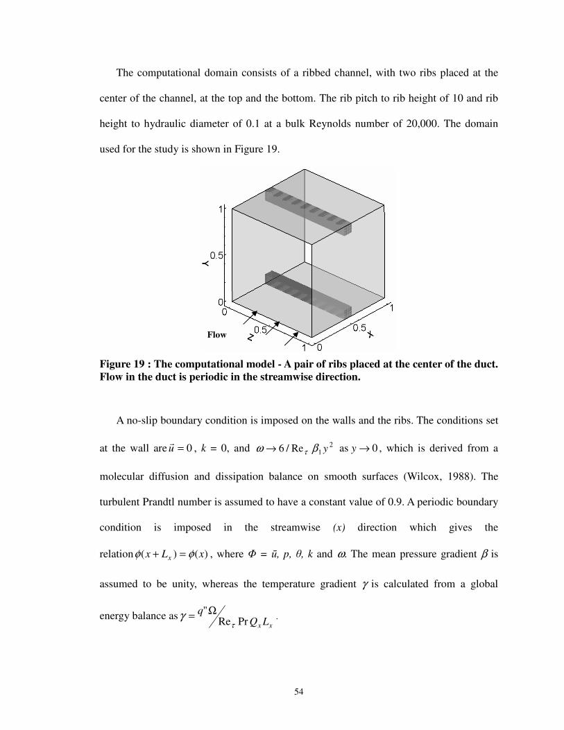
54

The computational domain consists of a ribbed channel, with two ribs placed at the

center of the channel, at the top and the bottom. The rib pitch to rib height of 10 and rib

height to hydraulic diameter of 0.1 at a bulk Reynolds number of 20,000. The domain

used for the study is shown in Figure 19.

Figure 19 : The computational model - A pair of ribs placed at the center of the duct. Flow in the duct is periodic in the streamwise direction.

A no-slip boundary condition is imposed on the walls and the ribs. The conditions set

at the wall are 0=u

, k = 0, and 21Re/6 yβω τ→ as 0→y , which is derived from a

molecular diffusion and dissipation balance on smooth surfaces (Wilcox, 1988). The

turbulent Prandtl number is assumed to have a constant value of 0.9. A periodic boundary

condition is imposed in the streamwise (x) direction which gives the

relation )()( xLx x φφ =+ , where = , p, , k and ω. The mean pressure gradient β is

assumed to be unity, whereas the temperature gradient γ is calculated from a global

energy balance asxx LQ

qPrRe

"τ

γ Ω= .

Flow

55

In the study, the flow and heat transfer in both stationary and rotating ducts is

investigated. The first section of the study deals with the detailed flow and heat transfer

validation in a stationary duct. This study is further extended in the subsequent sections

to study the effects of rotation. Initial computations are carried out by considering the

effects of Coriolis forces and neglecting the effects of centrifugal buoyancy to evaluate

the performance of DES in predicting the effects of Coriolis forces. Once these effects

have been successfully captured, the capability of DES in predicting the effects of

centrifugal buoyancy is validated.

5.1 Grid Sensitivity Comparisons

DES is sensitive to grid resolution as shown by earlier DES calculations (Forsythe et

al., 2002). The grid dependency is not similar to LES, where an increase in resolution of

the grid improves the solution. In DES, a grid which is fine might trigger an LES solution

in the boundary layer, which might be detrimental if the resolution is not fine enough for

LES. On the other hand, a coarse grid may eliminate the LES regions in the grid

altogether, and in the limit the calculation would default to a URANS calculation. So a

grid sensitivity study is carried out for the fully developed region of the stationary ribbed

duct.

Table 4: a-posteriori comparison of the grid dimensions in the three directions for the DES grids

0) 1 5 51

!0 ) 5 5

! 1 5! 5)

56

A 963 grid used for earlier LES studies (Tafti, 2005) was considered as the fine grid

used in the study. A baseline grid (643) was formed by maintaining the same grid

resolution near the walls and coarsening the grid in the inter-rib spacing and in regions

away from the channel walls. The coarsest grid (483 cells), was obtained by coarsening

the 643 grid in regions away from the walls. Henceforth, the 963, 643 and the 483 grids

are referred as fine grid, baseline grid, and the coarse grid, respectively. In the three

resolutions tested, the near wall grid resolution was maintained and only the regions away

from the wall were modified to generate coarser meshes. A a-posteriori grid evaluation

of the three grids is shown in Table 4.

(a) (b)

(c) (d)

Figure 20 : Comparison of the streamwise velocities in a plane through the ribs (y/e = 0.25) for the (a) 483 grid (b) 643 grid (c) 963 grid (d) LES 1283 case. 643 and the 963 case show the best agreement. 483 grid overpredits the extent of the recirculation region.

A non-dimensional time step of 5 x 10-5 was used in all the cases. Calculations are

initiated by assuming an initial bulk velocity and integrating in time until a balance

57

between the internal losses and the specified pressure gradient was obtained. Although

the whole domain is considered for the calculation, owing to the symmetry along the y

and z directions, the average solution for a quadrant is presented.

DES computations were carried out on the three grids and a comparison of the

average streamwise velocities (Figure 20) shows that while the baseline grid and the

dense grid compare well with the LES results, the coarse grid fails to accurately predict

the velocity levels. A comparison of the baseline grid and the denser grid shows that both

grids predict the streamwise velocity contours to good accuracy (Figure 20) and capture

the secondary recirculation behind the rib. The denser grid did not show any added value,

and so the baseline grid was considered to be sufficiently accurate for further study.

Hence, all computations have been carried out with the 643 (baseline) grid.

5.2 DES Regions

The underlying idea of DES is to compute regions closer to the wall using a RANS

model and solve the regions of separation, or the region of detached eddies, in LES mode.

Figure 21 shows the fraction of time (during the whole computation) when the

calculation is solved in the LES mode. DES uses a turbulent length scale which is

computed from the turbulence equations solved (k,ω). So the turbulent (RANS) length

scale is a function of time as well as space. This feature facilitates the computation to be

cognizant of the eddy length scales and hence behave as RANS or LES depending on the

instantaneous local conditions, unlike in the case of a Spalart – Allmaras based DES,

where DES acts just like a wall model. Another prominent feature of the DES version of

the two equation model is that although an instantaneous discontinuity may exist between

the RANS region and the LES region, in the mean however a smooth transition takes

58

place from RANS to LES and vice versa. It can be observed from Figure 21 that the

RANS regions transition into LES smoothly. In a DES Spalart - Allmaras model, the

distance from the wall determines the switch from RANS to LES, which is not as

receptive to instantaneous flow features.

DES

1.000.800.600.400.200.00

Figure 21 : Plot of the LES and RANS region in the DES computation for the 643 grid in a Z plane. A value of 1 represents a complete LES region and a value of 0 a complete RANS region. Flow is periodic in the streamwise direction.

The near wall region is always resolved in the RANS mode which transitions to the

LES mode as the distance from the wall increases. The flow in the vicinity of the ribs is

mostly resolved in LES mode all the way to the channel center. This includes the

unsteady large-scale dynamics of the separated shear layer as shown in Figure 21.

Though the inter-rib spacing is predominantly LES it transitions to a RANS mode at the

center of inter-rib region. The grid facilitates the computation of the region in RANS

and/or LES depending on the instantaneous conditions existing in the region.

Downstream of the rib, in the region of separation it is observed that the computation is

mostly carried out in the LES model. This sensitizes the RANS model to grid length

scales, thereby allowing the natural instabilities of the flow in this region to develop.

Thus the unsteady physics in the separated region is captured accurately.

59

5.3 Stationary Duct

5.3.1 Flow Field Predictions

The mean flow pattern observed in the symmetry plane of the span is shown in Figure

21. Flow patterns produced by the LES cases (Tafti, 2005), the RANS models (Ooi et al.,

2002) and the experiments (Rau et al., 1998), show a similar pattern. The flow is

characterized by a recirculating eddy in front of the rib, followed by shear layer

separation on the rib and the presence of a recirculation region on top of the rib and

behind it. Between the main recirculation region and the rib there is an additional

counter-rotating eddy. The reattachment length is calculated as 4.6e (for k-) and 4.1e

(for SST) from the rib, as compared to the LES predictions of 4.1e and experimentally

observed value of 4.0e – 4.25e. The prediction of the reattachment length is sensitive to

the level of turbulence in the separated shear layer, so the turbulence level may be under-

predicted in the k- case, due to which the reattachment length is over-predicted.

Table 5 : Percentage form and friction drag in the ribbed duct

LES 1283 DES k- DES SST RANS k-

Form Drag 91.0 91.9 95.2 88.0

Ribbed Wall Friction Drag -1.70 -1.80 -1.30 -1.40

Smooth Wall Friction Drag 7.80 4.50 3.20 11.80

Rib Friction -0.80 -0.17 -0.49 0.30

A comparison of the total drag in the duct shows that the form drag contributes to a

major part of the losses, as is evident from Table 5. The predicted values of form drag

agree well with the form loss measured by Rau et al., (1998) of around 85% and the LES

60

predictions of 91% by Tafti (2005). Owing to the recirculation, a negative friction loss is

observed at the ribbed walls of the duct. A small recirculation region was observed above

the rib by Rau et al. (1998). The DES calculations capture this recirculation while the k-

RANS calculation shows a smooth flow above the rib. This is evident from the negative

value of friction in the DES cases and a positive value in the RANS case (Table 5).

X

U/U

∞

0 0.2 0.4 0.6 0.8 1-0.4

-0.2

0

0.2

0.4MeasuredDES k-ωDES SSTRANS k-ωLES

Figure 22 : Streamwise velocity distributions at the center of the duct at y/e = 0.1 in comparison with the experimental measurements by Rau et al., (1998)

A plot of the normalized streamwise velocities (Figure 22) at a plane close to the

ribbed wall (y/e = 0.1) indicates the acceleration and deceleration of the flow in the inter-

rib region. The separated region behind the rib experiences a reverse flow, which is

evident from the negative velocities behind the rib up to the reattachment region. The

flow accelerates after reattachment and separates in front of the next rib, owing to the rise

in pressure. The separation in front and downstream of the rib are predicted by both DES

calculations (k- and Menter’s SST), and the velocity magnitudes are consistent with the

LES calculations and the measurements. The k- RANS fails to predict the flow

correctly in these regions.

61

(a) (b)

(c) (d)

Figure 23 : Comparison of streamwise velocity distributions at y/e = 0.25 for the (a) k- DES case (b) SST DES case (c) k- RANS case (d) LES case

A contour plot (Figure 23) of the streamwise velocities in a plane passing through the

rib (at y/e = 0.25) shows that the maximum velocities do not occur in the center of the

channel but closer to the side wall. The flow separation behind the ribs causes this shift.

While DES successfully reproduces the trend observed by the experiments, the k-

RANS case fails to capture the variation. Similar results were reported by Ooi et al,

(2002) for their RANS calculations. The DES distributions match well with the LES

cases (Tafti, 2005). The k- DES case over-predicts the separation region due to which

the zero velocity contour line is predicted further downstream as compared to LES and

Menter’s SST predictions.

Figure 24 shows the lateral w-velocities above the rib along a line close to the smooth

side wall (y/e = 1.5, z/Dh = 0.45), as an indication of the strength of the localized

secondary flow in the vicinity of the rib. The DES and the k- RANS calculations are

62

compared with the measured values and LES. While RANS completely fails at resolving

this feature of the flow, DES does a good job at resolving the correct distribution.

x

w/U

∞

0 0.2 0.4 0.6 0.8 1-0.20

-0.10

0.00

0.10Exp. Rau et alLESDES k-ωDES SSTRANS k-ω

Figure 24 : Comparison of the secondary flow distribution at y/e = 1.5 and z/Dh = 0.45

Mean secondary flow patterns in the cross-section were studied experimentally by

Liou et al. (1993) using LDV techniques. These secondary flow structures are strongest

in the vicinity of the ribs and are generated by turbulence. The flow causes core fluid in

the center of the duct to be drawn towards the side walls. The impinging secondary flow

has a large effect on enhancing heat transfer. Ooi et al. (2002) reported a large

inconsistency between the k- RANS calculations and the experimental observations,

resulting in large disagreement between the experimentally measured and the calculated

side wall heat transfer. A similar discrepancy in the prediction of the secondary flow was

observed in the k- RANS calculation. But the DES versions of the k- and the SST

models predicted the secondary structures (Figure 25). Near the center of the channel

there is a flow towards the ribbed walls. The flow turns near the corners and moves along

the smooth walls towards the center of the channel.

63

(a) (b)

(c) (d)

Figure 25 : Comparison of the secondary flow (a) predicted by DES k- model (b) DES SST model (c) k- RANS model (d) Experimental (Liou et al.).

Table 6 : Comparison of the overall friction factor.

LES 1283 DES k- DES SST RANS k- Rau et al.

f/f0 8.60 9.30 9.56 8.76 9.50

The average friction factor augmentation ratios summarized in Table 6 give an

estimate of the additional pressure loss incurred due to the introduction of the ribs in the

duct. The average friction factor predicted by the DES schemes is very close to the

experimentally measured values, and is within an accuracy of 2.5%. The k- RANS

64

calculation predicts a value which is within acceptable limits, even though the localized

predictions are not accurate. This is due to the over-predictions in some regions

compensating for other localized under-predicted values.

Figure 26 : Streamlines showing the recirculation region in front of the rib and primary and secondary circulations behind the rib and their effect on heat transfer on the walls. Red regions represent high heat transfer, while blue regions represent low heat transfer.

5.3.2 Heat Transfer Enhancement

Figure 26 shows the distribution of heat transfer augmentation at the ribbed wall and

the smooth walls of the duct. The augmentation ratio is high in front of the rib as a result

of the unsteady junction vortices in this region. These secondary vortices continuously

transport cooler fluid from the mainstream to the ribbed wall increasing the heat transfer

coefficient. Immediately behind the rib, a secondary recirculation is trapped between the

wall and the primary recirculation zone. Although the action of the secondary eddy

causes some localized augmentation in this region, the overall augmentation is low and

similar to that in a smooth duct. Further downstream, the heat transfer coefficient

increases steadily as the vortices from the separated shear layer impinge on the wall. The

65

heat transfer reaches a maximum value at about 3.5e downstream of the rib, which is

upstream of the mean reattachment line and coincides with the region of maximum shear.

In the spanwise direction, the heat transfer does not show much variation. However, on

moving closer to the smooth walls the heat transfer augmentation drops and the minimum

heat transfer is observed at the corners formed by the ribbed and the smooth walls. Heat

transfer augmentation on the smooth walls is dominated by secondary flow impingement

at the top upstream corners of the rib, and decreases towards the center of the channel.

(a) (b)

(c) (d)

Figure 27 : Comparison of augmentation ratios on the ribbed floor for the (a) k- DES case (b) Menter's SST DES case (c) k- RANS case (d) LES case

The distribution of augmentation ratios on the ribbed wall is plotted in Figure 27 and

in Figure 28(a) along the centerline. Both DES calculations are consistent with LES and

experiments in reproducing the spatial distribution of augmentation ratios, whereas the

distribution predicted by RANS is quite different. RANS fails to resolve the secondary

eddy behind the rib and its associated effect on augmentation. It also fails to resolve the

high augmentation at the front of the rib. These shortcomings can be clearly identified in

66

Figure 28(a) at the center of the channel, in which the augmentation predicted by RANS

immediately before and after the rib is much lower than the other methods. Ooi et al.

(2002) observed a similar trend. Both DES calculations resolve these features, with the

Menter’s SST model predicting a solution closer to the experimental measurements. The

RANS calculation, in spite of severe shortcomings in predicting the salient features,

predicts the augmentation in the inter-rib spacing quite well.

x

Nu

/Nu 0

0 0.2 0.4 0.6 0.8 10

1

2

3

4

5Rau et alLESDES k-ωDES SSTRANS k-ω

Nu / Nu0

Y

1 2 3 40

0.1

0.2

0.3

0.4

0.5 Rau et alLESDES k-ωDES SSTRANS k-ω

(a) (b)

Figure 28 : Comparison of the augmentation ratios (a) at the center of the ribbed floor (b) side walls upstream of the rib

While the heat transfer on the ribbed wall is enhanced due to the streamwise flow, the

secondary flow impingement plays a major role in the heat transfer on the side walls.

Predictions on the smooth side walls also show the inefficiency of linear eddy-viscosity

RANS in Figure 28(b) and Figure 29. The k- RANS calculation fails to capture the

augmentation at the upstream corner of the rib which is caused by the secondary flow

impingement. On moving away from the ribbed walls the enhancement ratio is almost

constant in k- RANS, in contrast to the experimental observations, in which the heat

transfer decreases on moving towards the center of the channel. The DES predictions

67

capture the high heat transfer near the rib and also show the decreasing trend in heat

transfer.

(a) (b)

(c) (d)

Figure 29 : Comparison of the heat transfer augmentation ratios on the side walls (a) k- DES (b) Menter’s SST DES (c) k- RANS (d) LES

Table 7 shows the surface averaged augmentation ratios at the ribbed wall, smooth

wall and the ribs in comparison to experimental values. All prediction techniques are

within 10% of the experiments. However, it is noted that the good agreement of the k-w

RANS model is fortuitous and is brought about by a cancellation of errors.

Table 7 : Comparison of the overall heat transfer augmentation

LES 1283 DES k- DES SST RANS k- Rau et al.

Ribbed Wall 2.40 2.17 2.35 2.14 2.40

Error 0.0% 9.4% 2.1% 10.6%

Side Wall 1.89 1.89 1.86 1.83 2.05

Error 7.7% 7.7% 9.2% 10.8%

Ribs 2.89 2.40 2.41 2.38

68

5.3.3 Summary and Conclusions

DES and RANS computations are presented in a square duct with normal ribs. The

domain is discretized using a 643 grid and the computations are compared to the

experimental flow and heat transfer results obtained by Rau et al. (1998) and LES

computations by Tafti (2005).

From the computations performed, the following conclusions can be derived:

1. The average flow characteristics are predicted with good accuracy by the DES

computations. DES accurately captures the recirculation regions in front of the rib,

behind the rib, and on top of the rib. Owing to the accurate prediction of the main flow

characteristics, the heat transfer on the ribbed wall, which is influenced mostly by the

main flow, is also predicted with good accuracy.

2. The secondary flow is also accurately captured by the DES computations, while the

k- RANS fails to capture the secondary flow. Consequently, the heat transfer

augmentation on the side walls is predicted with good accuracy by DES, whereas the k-

RANS calculation fails to accurately capture the side wall heat transfer.

3. The overall flow characteristics and heat transfer predicted by DES agree well with

the LES computations and the experimental results, at approximately one-tenth the

computational cost of LES.

4. RANS models with known limitations perform better in the DES framework than

they would normally in the RANS or URANS framework.

5. By directly resolving more of the turbulent energy, DES, as with LES, is less

dependent on the base RANS modeling capability.

69

5.4 Rotating Duct - Effects of Coriolis Forces

Early studies in turbulent channel flow (Halleen & Johnston, 1967; Lezius &

Johnston, 1976) have established two important effects of rotation. When the rotational

axis is perpendicular to the plane of mean shear, Coriolis forces have a considerable

effect on the mean flow as well as on turbulent fluctuations. These effects are manifested

as stabilization/destabilization of turbulence at leading/trailing walls and the generation

of spanwise roll cells or secondary flow patterns. The secondary flow patterns are a direct

result of the action of Coriolis forces on mean shear and are also observed in laminar

flows subjected to system rotation.

Figure 30: Effect of Coriolis forces in a square duct subjected to rotation

It is well established that the production of turbulence in the near wall region and in

shear layers is caused by the exchange of momentum through intense interactions

between the fluctuating streamwise and cross-stream velocities. When Coriolis forces act

70

in tandem with these events, turbulence is augmented, whereas it is attenuated when the

two act in opposition. Due to the vector nature of the momentum equations the flow

direction determines this bias in the effects of turbulence. The effects of Coriolis forces in

a rotating duct are shown in Figure 30. When the direction of the flow is outwards, as

considered in the ribbed duct flow in this study, both the turbulent shear layer and near

wall turbulence on the trailing surface are augmented by the direct effect of Coriolis

forces, while the opposite effect comes into play at the leading wall.

Modern propulsion turbines used in aircrafts rotate at a non-dimensional rotation

number of around 0.2. Gas turbines used for power generation have a higher rotation rate

(Ro = 0.5 – 1.0), as compared to the aircraft engines. In the study three rotation numbers

– Ro = 0.18, 0.35 and 0.67 are examined which cover a wide range of turbine

applications. The results obtained using DES are evaluated against the detailed results

obtained from LES (Abdel-Wahab and Tafti, 2004).

5.4.1 Mean Flow field

The flow at the center (z=0.5) of the duct is characterized by a large recirculation

region behind the rib, a small region of recirculation in front of the rib, a small eddy on

top of the rib and an eddy trapped behind the rib, between the large recirculation region

and the rib. For a non-rotating case all these features are similar on both the ribbed walls.

71

(a) (b)

(c)

Figure 31: Streamlines showing the flow in a fully developed duct as predicted by DES SST at Z = 0.5 (a) Ro = 0.18 (b) Ro = 0.35 (c) Ro = 0.67. Y = 0 represents the trailing wall, while Y = 1 represents the leading wall. Flow direction is from left to right.

Figure 31 shows the streamlines at the center of the duct (z = 0.5) for the three

rotation cases. Rotational Coriolis forces affect the size of the recirculation zones and so

the flow is asymmetric about the center y-plane of the duct. The reattachment length

increases at the leading wall and decreases at the trailing wall with rotation number. The

72

reattachment is observed at around 4.0e for Ro = 0.18 at the trailing side. The size of the

separation bubble decreases to a value close to 3.6e when the rotation increases to 0.35.

On increasing the rotation further to 0.67 the reattachment length remains almost the

same as the 0.35 case. On the other hand, the reattachment length at the leading wall

increases from a value of 4.25e for the stationary case (Ro = 0.0) to a value of 4.5e at Ro

= 0.18. No significant change is observed as the Ro is increased to 0.35, but on increasing

the rotation further to 0.67, the recirculation region is observed to increase to a value of

around 6.7e, and as a result it almost merges with the recirculation region in front of the

next rib.

The reattachment lengths for the rotating cases are consistent with the LES

predictions (Abdel-Wahab et al., 2004). Figure 32 shows the comparison of the flowfield

as predicted by LES, DES and URANS. The separation and reattachment downstream of

the rib is predicted accurately by DES and the reattachment length is in agreement with

LES both at the leading and the trailing walls. However URANS overpredicts the

reattachment lengths both at the leading as well as the trailing wall. Overprediction of the

reattachment lengths is a result of the inability of the SST model to account for the effects

of Coriolis forces, whereas in DES, the effect of Coriolis forces is captured in the

resolved scales.

73

(a) (b)

(c)

Figure 32: Streamlines showing the flow in a fully developed duct rotating at Ro = 0.35 at Z = 0.5 as predicted by (a) LES (b) DES SST (c) URANS SST. Y = 0 represents the trailing wall, while Y = 1 represents the leading wall. Flow direction is from left to right.

Figure 33 shows the magnitude of the secondary flows (v, w velocities) for the

stationary and the three rotation cases in the cross-section of the duct on top of the rib.

The v- and w- velocities are plotted individually in each half of the span. Above the rib,

the constriction posed by the rib results in flow being pushed towards the channel center,

74

both at the center of the span and near the side wall. In addition to this effect, a spanwise

flow is setup toward the center and toward the side wall which is represented by the high

positive impingement w-velocities at the side wall. As rotation increases, the strength of

the secondary impingement flow at the trailing side increases while it decreases at the

leading side, which is evident from the penetration of the high v-velocities towards the

leading side near the side wall. The asymmetry in the w-velocity slightly increases as the

rotation increases.

(a) (b)

(c) (d)

Figure 33: Secondary flow contours on the rib for (a) Ro = 0.0 (b) Ro = 0.18 (c) Ro = 0.35 (d) Ro = 0.67 as predicted by DES SST. The contours show the effect of rotation on the secondary flow in the cross-section.

75

5.4.2 Turbulent Flow Characteristics

A comparison of the turbulent kinetic energies (TKE) predicted by the DES, LES and

the URANS schemes are shown in Figure 34. The resolved component of TKE is

considered for comparison for the LES cases, while the sum of the resolved and the

modeled components are considered for the DES and URANS cases. It is observed that

the resolved component of TKE is significantly larger than the modeled component in the

DES computation almost in the entire flow field. On the other hand the resolved and the

modeled components make equal contributions in URANS.

k

Y

0 0.1 0.2 0.30

0.2

0.4

0.6

0.8

1

Ro = 0.18 DESRo = 0.18 LESRo = 0.18 URANS

k

Y

0 0.1 0.2 0.30

0.2

0.4

0.6

0.8

1


k

Y

0 0.1 0.2 0.30

0.2

0.4

0.6

0.8

1


Rotation

k

Y

0 0.1 0.2 0.30

0.2

0.4

0.6

0.8

1


k

Y

0 0.1 0.2 0.30

0.2

0.4

0.6

0.8

1


k

Y

0 0.1 0.2 0.30

0.2

0.4

0.6

0.8

1


Rotation

Figure 34: TKE values as predicted by the DES, LES and the URANS cases for the three rotation cases at z = 0.5 and x = 0.65, i.e., 1e downstream of the rib.

A comparison of the TKE in between the rib shows that the values resolved by DES

compare well with that resolved by LES for all the three rotation cases. The plotted

location is one rib distance downstream of the rib and so represents the separation region

for all the three cases both at the trailing and the leading sides. The turbulence statistics in

the vicinity of the wall (Y < 0.1) region determine the reattachment point downstream

and the heat transfer at the ribbed walls. It is observed that the TKE values predicted in

the boundary layer by DES compared well to LES for all the other rotation cases. On the

other hand, URANS underpredicts the TKE values in this region for all the cases. The

76

low turbulence levels in URANS results in larger recirculation regions as compared to

DES and LES.

(a) (b)

(c)

Figure 35: Coherent vorticity contours for the (a) LES 1283 (b) DES 643 (c) URANS 643 for Ro = 0.35 show the scales resolved of the three schemes. The flow in all cases is from left to right

A comparison of the instantaneous coherent vorticity (Chong et al, 1990) as predicted

by 1283 LES, 643 DES and 643 URANS is shown in Figure 35. These plots give an idea of

the flow structures resolved by the three schemes. It is observed that the magnitude of

coherent vorticity and the characteristics predicted by DES is consistent with the

magnitudes predicted by LES on a much finer grid. Predictions by URANS show lower

vorticity levels as compared to LES and DES, both in the center of the duct as well as the

77

inter-rib region. Thus the small modification in the URANS model to convert it into an

equivalent DES model substantially improves the resolution of the simulation.

5.4.3 Mean Heat Transfer

(a) (b) (c)

Figure 36: Heat transfer augmentation (Nu/Nu0) predicted at the leading and the trailing walls by DES SST for (a) Ro = 0.18 (b) Ro = 0.35 (c) Ro = 0.67. Flow direction is from left to right.

The heat transfer trends at the leading and trailing walls are similar to the trends

observed at the ribbed walls for the stationary case. The augmentation ratio is high in front

of the rib as a result of the unsteady vortices in this region. These secondary vortices

continuously transport cooler fluid from the mainstream to the ribbed wall increasing the

heat transfer coefficient. Immediately behind the rib, a secondary recirculation is trapped

between the wall and the primary recirculation zone. Although the action of the secondary

eddy causes some localized augmentation in this region, the overall augmentation is low

and similar to that in a smooth duct. Further downstream, the heat transfer coefficient

increases steadily as the vortices from the separated shear layer impinge on the wall.

Figure 36 shows the heat transfer at the leading (upper half) and the trailing walls

(lower half) for the three rotation cases. As the rotation number is increased, an increase

78

in the heat transfer is observed at the trailing wall, especially in regions immediately

upstream of the rib and near the reattachment point. This is countered by a decrease at the

leading wall in the corresponding regions.

(a) (b) (c)

Figure 37: Heat transfer augmentation (Nu/Nu0) predicted at the leading (upper half of the plot) and the trailing walls (lower half of the plot) for the Ro = 0.35 case by (a) LES (b) DES SST(c) URANS SST. Flow direction is from left to right.

Figure 37 shows a comparison of the DES and the URANS with LES results at

Ro=0.35. This shows that the URANS under-predicts the heat transfer at the trailing side

where the turbulence is enhanced by rotation. The heat transfer augmentation predicted

by DES agrees quite well with the LES computations. The peak heat transfer on the

trailing wall in the region of shear layer reattachment is shifted away from the center of

the duct due to the effect of secondary flows and is captured by all three methods.

However, the URANS predicts this region further downstream because of the larger

reattachment length. Heat transfer augmentations at the trailing wall reach values close to

5.0 immediately upstream of the rib where the unsteady vortices enhance the heat

transfer. Both DES and URANS tend to over-predict the spatial extent of this region.

The flow at the leading wall is more stable than the flow at the trailing wall and so the

overall heat transfer at the leading wall is almost half the heat transfer at the trailing wall.

79

Upstream of the rib, heat transfer levels are almost 2.5 times that observed in a smooth

duct case. Once again, both DES and URANS overpredict the extent and augmentation in

this region. The heat transfer levels drop to values close to the smooth channel heat

transfer values immediately behind the rib, but the augmentation increases to values close

to 1.5 downstream of the reattachment point.

The trends predicted by DES are consistent with the LES results (Abdel-Wahab et al.,

2004), with the exception of the region immediately upstream of the rib where higher

levels of heat transfer are predicted. Similar results were observed in a stationary duct

where a larger heat transfer augmentation was observed immediately upstream of the rib.

On the other hand URANS results show a lot of discrepancy. The most prominent

deviation from LES is the under-prediction of the heat transfer at the trailing wall of the

duct. The heat transfer distributions at the ribbed walls are also much smoother than LES

and DES predictions.

The secondary flows in the stationary and the rotation cases play an important role in

the heat transfer at the side walls. Along the smooth (side) walls the heat transfer

increases on moving from the trailing wall and reaches a maximum at the top front corner

of the rib as a result of the secondary flow impingement on the wall. The heat transfer

decreases on the side walls towards the center of the channel. Though the heat transfer

patterns are the same for the stationary and the rotation cases the magnitudes of heat

transfer are higher when rotation is introduced.

80

(a) (b) (c)

Figure 38: Heat transfer augmentation (Nu/Nu0) predicted at the side wall by DES SST for the (a) Ro = 0.18 (b) Ro = 0.35 (c) Ro = 0.67. Flow direction is from left to right.

For Ro = 0.18 (Figure 38) the secondary flow impingement results in levels of heat

transfer as high as seven times that in a smooth channel at the trailing wall, at the corner

of the rib and the side wall. The heat transfer decreases to values close to 2.0 towards the

center of the duct. On moving towards the leading side the heat transfer decreases further

and drops to values close to unity near the leading wall of the side wall. However

secondary flow impingement near the corner of the ribs locally results in higher heat

transfer. An increase in rotation does not show much effect on the side wall heat transfer.

This behavior is consistent with the observations of Wagner et al., (1992) who observed

little or no changes in the heat transfer at the side walls as rotation rate increases.

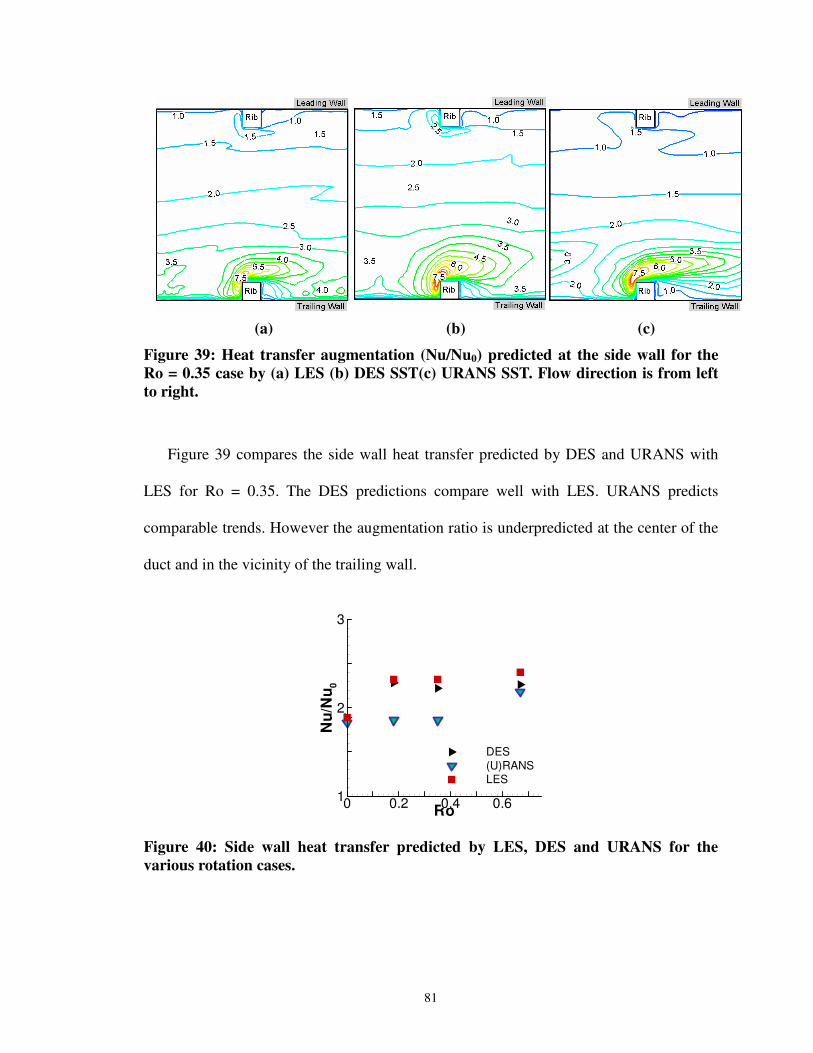
81

(a) (b) (c)

Figure 39: Heat transfer augmentation (Nu/Nu0) predicted at the side wall for the Ro = 0.35 case by (a) LES (b) DES SST(c) URANS SST. Flow direction is from left to right.

Figure 39 compares the side wall heat transfer predicted by DES and URANS with

LES for Ro = 0.35. The DES predictions compare well with LES. URANS predicts

comparable trends. However the augmentation ratio is underpredicted at the center of the

duct and in the vicinity of the trailing wall.

Ro

Nu/

Nu 0

0 0.2 0.4 0.61

2

3

DES(U)RANSLES

Figure 40: Side wall heat transfer predicted by LES, DES and URANS for the various rotation cases.

82

Figure 40 shows a gradual, but small increase in the average heat transfer

augmentation at the side walls as the rotation number increases from 0.18 to 0.67. DES

predicts these trends accurately but slightly underpredicts the augmentation compared to

LES at higher rotation rates. URANS severely underpredicts the side wall heat transfer at

Ro = 0.18 and 0.35, while the agreement is comparatively better at the highest rotation

number.

Ro

Nu/

Nu 0

0 0.2 0.4 0.60

1

2

3

4

5

6Liou et al.Wagner Bo = 0.04Parsons et al.LESDESURANSTrailing Side

Leading Side

Figure 41: Comparison of average Nusselt number augmentation ratios at the leading and trailing sides with experiments.

The effect of rotation is more prominent at the leading and the trailing walls. Results

for averaged Nusselt numbers on the leading and trailing faces for the three rotation

numbers are compared with the experiments of Liou et al. (2001), Parsons et al. (1994),

and Wagner et al. (1992). The experimental data of Liou et al. (2001) is at Re = 10,000

for e/Dh = 0.136 and P/e = 10 and Parsons et al. (1994) data is obtained at Re=5,000 for

e/Dh = 0.125 and P/e = 10. The data of Wagner et al. (1992) includes the effects of

buoyancy with a density ratio = 0.13 for a staggered rib arrangement with e/Dh = 0.1 and

P/e = 10 at Re=25,000. Wagner’s data includes the effects of centrifugal buoyancy which

increase trailing wall heat transfer as the rotation number increases. In all cases, fully-

83

developed data is extracted for comparison. Figure 41 compares the overall heat transfer

augmentations at the leading and trailing walls predicted by DES and URANS cases, with

the LES computations and experimental results. DES predictions agree well with

experiments and LES. On the other hand, URANS substantially underpredicts the trailing

wall augmentation, by as much as 30% compared to LES, at the high rotation numbers of

0.35 and 0.67. Prediction accuracy of URANS is similar to that of DES at the leading

wall which is within 10% of LES.

5.4.4 Conclusions

Results from DES and URANS of a fully developed flow in a 90° ribbed duct are

presented for three rotation cases – Ro = 0.18, 0.35 and 0.67 at a Reynolds number of

20,000. The computations were performed on a 643 mesh tested earlier for a stationary

case which is almost an order of magnitude less expensive than the analogous LES

computation (Abdel-Wahab and Tafti, 2004).

The effect of rotation is observed by an increase in the turbulence intensity at the

trailing wall due to which the reattachment length decreases. Secondary flow

impingement is observed to become stronger as rotation increases. These flow features

result in an increase in the heat transfer at the trailing wall. The peak heat transfer level

increases from a value of about 3.0 for the stationary duct to a value of about 6.0 for the

largest rotation. The overall heat transfer at the trailing wall increases by almost a factor

of 1.5 as the system is rotated from rest to Ro = 0.67.

At the leading wall the opposite effect is observed. Rotation damps turbulence at the

leading wall resulting in larger recirculation regions. It is observed that the recirculation

region downstream of the rib almost overlaps the recirculation region upstream of the

84

next rib. This results in low levels of heat transfer at the leading wall. The heat transfer

distribution drops to values close to that in a smooth duct for the highest rotation

considered.

The heat transfer at the side walls show distributions similar to a stationary duct. The

heat transfer is high at the corner of the rib, which is due to the impingement of the

secondary flows on the side walls. The heat transfer decreases on moving from the

trailing wall to the leading wall. Rotation increases the magnitude of the secondary flows

and increases the heat transfer augmentation on the side walls.

The flow and heat transfer distribution predicted by the DES SST case is consistent

with the LES predictions. Though higher heat transfer is predicted immediately upstream

of the rib, the distribution in the other regions is accurate. The overall predicted heat

transfer also match well with the LES predictions and the experimental observations.

URANS fails to capture the effects of the Coriolis forces at the trailing wall and

underpredicts the heat transfer.

In summary, it is concluded that DES accurately predicts the physics of the rotation

dominated flow, in addition to accurately predicting separation and reattachment and

unsteady vortex induced secondary motions. The main contribution of this work is in

establishing that DES, like LES, can produce quality results at a cost which is an order of

magnitude less than an equivalent LES. It is also observed that the URANS model when

used in a DES mode overcomes the deficiency of the base model and predicts the effects

of shear and rotation in the flow and heat transfer in the fully developed region of the

internal cooling duct.

85

5.5 Rotating Ducts - Effects of Coriolis Forces and Centrifugal

Buoyancy

The study of the flow and heat transfer in rotating ducts, considering the effects of the

Coriolis forces and neglecting centrifugal buoyancy shows that URANS fails to capture

the effects of rotation. However, RANS when applied in the DES mode captures the

effects of rotation. Since the application of DES in capturing the effects of Coriolis forces

has been validated, the next step is to test and validate the capabilities of DES in

predicting the flow and heat transfer in internal cooling passages when the centrifugal

buoyancy effects introduced by the temperature difference at the trailing and leading

walls of the passage become significant. The advantage of applying DES is two-fold – to

cut down the computational cost associated with LES and to eliminate the deficiencies

observed in using standard eddy viscosity RANS models. The main objective of this part

of the study is to validate the performance of DES in capturing the mixed convection

effects introduced in the flow in a ribbed duct due to the action of shear, rotation and

buoyancy.

In the cases studied three different rotation cases are considered – Ro = 0.18, 0.35 and

0.67. Three different density ratios are studied to evaluate the capability of DES in

predicting the effects of buoyancy. The effective buoyancy numbers (Bo) for the three

cases are evaluated to be 0.00, 0.12 and 0.29 respectively. In the present context the

density difference and the buoyancy number are related as 2

0

RoDr

Bohρ

ρ∆= . In all the

cases the centrifugal buoyancy complements the effects of Coriolis forces. In typical gas

turbine applications the buoyancy parameters can reach values of upto 1.0. However

86

since detailed LES results (Abdel-Wahab and Tafti, 2004) are available for the buoyancy

parameters in the range of 0.00 – 0.30, the current studies are carried out for the relevant

density ratios.

The detailed flow and heat transfer physics is compared with LES prediction by

Abdel-Wahab and Tafti (2004) on a 1283 grid. Considering the grid sizes and the time

scales used for the LES and DES calculations, the cost of the DES computation is almost

an order of magnitude less than the LES computation (Abdel-Wahab and Tafti, 2004).

The surface averaged heat transfer augmentation has been validated with heat transfer

data from Wagner et al., (1992) and the LES computation (Abdel-Wahab and Tafti,

2004).

5.5.1 Effects of Centrifugal Buoyancy

Figure 42: Effect of Coriolis forces (F) and Centrifugal Buoyancy (Fb) in rotating ducts

87

Rotation induces Coriolis forces that accentuate the turbulence and destabilizes the

flow on one side and attenuates turbulence and stabilizes the flow at the other side. This

has a direct effect on the heat transfer at the ribbed walls. Due to the vector nature of the

equations of motion, the flow direction has a significant influence on the effects of

Coriolis forces and Centrifugal buoyancy. When the flow is radially outwards, the heat

transfer at the trailing wall is observed to be higher than the heat transfer at the leading

wall (Figure 42). The opposite trend is observed when the flow is radially outwards.

Section 5.4 which studies the effect of Coriolis forces on radially outward flows show

that as the rotation in the duct is increased to a value of Ro = 0.67, the rib averaged heat

transfer increases by a factor of around 65% as compared to the stationary duct at the

trailing wall. On the other hand the heat transfer at the leading wall decreases by a factor

of around 75%. This difference in the heat transfer results in the fluid near the leading

wall to be warmer than the fluid at the trailing wall. Difference in the densities of the

fluids in the vicinity of the ribbed walls induces centrifugal buoyancy. In the radially

outward flow considered the centrifugal buoyancy aids the effects of Coriolis forces.

5.5.2 Mean Flow Features

Studies in the hydrodynamically and thermally fully developed flow in a ribbed duct

show that as rotation is increased the separation region at the leading side increases in

size, while it decreases at the trailing side. While the size of the recirculation region

downstream of the rib at the trailing side reaches a constant value as the rotation

increases, considerable changes in the reattachment lengths are observed at the leading

wall. Figure 43 shows the comparison of the reattachment lengths at the center (z =

0.5Dh) of the leading wall for the three rotation cases. The effects of rotation for a

88

constant buoyancy number (Bo = 0.12) is shown. It is observed that as the rotation is

increased from 0.18 to 0.67, the reattachment length increases from a value of around 5e

to a value of 8.5e at the leading surface.

Comparison of the recirculation regions for the three rotation cases with predictions

by LES show that the recirculation regions for Ro = 0.18 and 0.35 are consistent with the

predictions by LES. The recirculation region predicted for the highest rotation case is

slightly different. The effective rotation number for the largest rotation case is around

0.74 as compared to the value of 0.67 used for the DES case, which could potentially lead

to the difference in the reattachment lengths.

Figure 43: Comparison of the recirculation regions at the leading edge for the three rotation cases with Bo = 0.12.

Centrifugal buoyancy, like Coriolis forces affects the recirculation region at the

leading wall. Figure 44 shows the recirculation regions at the leading wall for a constant

rotation rate of Ro = 0.35 and different buoyancy numbers. It is observed that as the

buoyancy number is increased from a value of Bo = 0.00 to Bo = 0.29, the recirculation

89

region grows until one large recirculation zone is observed at the leading wall for Bo =

0.29.

Figure 44: Comparison of the recirculation regions at the leading edge for the three different buoyancy cases with Ro = 0.35.

A comparison with LES shows concurrence. The structure of the recirculation regions

for Bo = 0.00 and 0.12 are reproduced by DES. For Bo = 0.29, while one large

recirculation region is observed in between the ribs, the structure of the recirculation

regions is different as predicted by LES and DES.

The effects of Coriolis forces on the secondary flow in the duct cross-section showed

an increase in the vertical velocity as the rotation is increased. Figure 45 shows the effect

of buoyancy on the secondary flows for the rotation number of Ro = 0.35. The magnitude

of the secondary flows (v, w velocities) for the stationary and the three rotation cases in

the cross-section of the duct on top of the rib are shown and the v- and w- velocities are

plotted individually in each half of the span. A strong component of vertical velocity is

observed in the vicinity of the side walls. At the core of the channel, a milder upwash is

observed which propagates upwards as the buoyancy is increased. This can be observed

from the movement of the zero vertical velocity contour line from the lower half of the

90

duct towards the upper half as buoyancy number is increased. So as buoyancy increases,

the cross-stream flow results in a tendency of the fluid to accumulate at the leading

surface.

(a) (b)

(c)

Figure 45: Comparison of the secondary velocities for Ro = 0.35 for varying buoyancies (a) Bo = 0.00 (b) Bo = 0.12 (c) Bo = 0.29

Very small differences are observed in the lateral velocity components in the duct as

the buoyancy number is increased. Positive velocities represent flow toward the side wall

while negative velocities represent flow towards the core of the duct. A high lateral

velocity is observed near the rib – side wall junction at the trailing wall. The magnitude

of this high velocity is observed to be almost constant as the buoyancy is increased. This

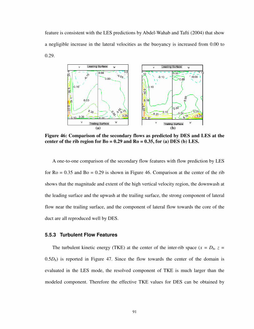
91

feature is consistent with the LES predictions by Abdel-Wahab and Tafti (2004) that show

a negligible increase in the lateral velocities as the buoyancy is increased from 0.00 to

0.29.

(a) (b)

Figure 46: Comparison of the secondary flows as predicted by DES and LES at the center of the rib region for Bo = 0.29 and Ro = 0.35, for (a) DES (b) LES.

A one-to-one comparison of the secondary flow features with flow prediction by LES

for Ro = 0.35 and Bo = 0.29 is shown in Figure 46. Comparison at the center of the rib

shows that the magnitude and extent of the high vertical velocity region, the downwash at

the leading surface and the upwash at the trailing surface, the strong component of lateral

flow near the trailing surface, and the component of lateral flow towards the core of the

duct are all reproduced well by DES.

5.5.3 Turbulent Flow Features

The turbulent kinetic energy (TKE) at the center of the inter-rib space (x = Dh, z =

0.5Dh) is reported in Figure 47. Since the flow towards the center of the domain is

evaluated in the LES mode, the resolved component of TKE is much larger than the

modeled component. Therefore the effective TKE values for DES can be obtained by

92

considering the TKE resolved by the sub-grid scales. While comparisons have been

carried out with LES, the effect of rotation and buoyancy are simultaneously studied.

k

Y

0 0.1 0.2 0.3 0.4 0.50

0.2

0.4

0.6

0.8

1

DES Ro = 0.35LES Ro = 0.35

kY

0 0.1 0.2 0.3 0.4 0.50

0.2

0.4

0.6

0.8

1

DES Ro = 0.18LES Ro = 0.18

k

Y

0 0.1 0.2 0.3 0.4 0.50

0.2

0.4

0.6

0.8

1

DES Ro = 0.67LES Ro = 0.67

k

Y

0 0.1 0.2 0.3 0.4 0.50

0.2

0.4

0.6

0.8

1

DES Bo = 0.00LES Bo = 0.00

k

Y

0 0.1 0.2 0.3 0.4 0.50

0.2

0.4

0.6

0.8

1

DES Bo = 0.29LES Bo = 0.29

Rot

atio

nBuoyancy

Bo = 0.12

Ro

= 0.

35

k

Y

0 0.1 0.2 0.3 0.4 0.50

0.2

0.4

0.6

0.8

1

DES Ro = 0.35LES Ro = 0.35

kY

0 0.1 0.2 0.3 0.4 0.50

0.2

0.4

0.6

0.8

1

DES Ro = 0.18LES Ro = 0.18

k

Y

0 0.1 0.2 0.3 0.4 0.50

0.2

0.4

0.6

0.8

1

DES Ro = 0.67LES Ro = 0.67

k

Y

0 0.1 0.2 0.3 0.4 0.50

0.2

0.4

0.6

0.8

1

DES Bo = 0.00LES Bo = 0.00

k

Y

0 0.1 0.2 0.3 0.4 0.50

0.2

0.4

0.6

0.8

1

DES Bo = 0.29LES Bo = 0.29

Rot

atio

nBuoyancy

Bo = 0.12

Ro

= 0.

35

Figure 47: Comparison of the turbulent kinetic energy in between two consecutive ribs at z = 0.5.

With an increase in rotation, the TKE value at the trailing surface is observed to

increase as Ro is increased from 0.18 to 0.35. However, as the rotation is increased to a

value of 0.67, the peak TKE value at the trailing surface decreases. At the leading surface

the peak turbulent kinetic energy is observed to be almost constant. The TKE profiles

predicted by DES compare well with the profiles predicted by LES, except for the largest

rotation case where the TKE at the core of the duct is observed to be over-predicted as

compared to LES. The TKE is underpredicted in the boundary layer as the near wall

93

region is modeled using URANS and the modeled component of TKE is a significant part

of the total TKE.

As the buoyancy is increased from a value of Bo = 0.00 to Bo = 0.12 it is observed

that the peak TKE at the trailing surface increases from a value of around 15% to about

22%. A corresponding decrease in the TKE is observed at the leading surface where the

TKE value drops from a value of around 9% to a value of 7%. Little difference is

observed in the value of the peak TKE values at the leading and trailing surfaces as the

buoyancy is increased to Bo = 0.29. The trends and the TKE profiles match well with

LES.

5.5.4 Heat Transfer Augmentation

Rotation augments the heat transfer at the trailing surface and decreases the heat

transfer at the leading surface. From the comparison of the heat transfer for varying

rotation cases (for a zero buoyancy case) it was observed that as the rotation increases,

the heat transfer at the trailing surface increases, and the heat transfer at the leading

surface decreases correspondingly.

X

Nu/

Nu 0

0 0.2 0.4 0.6 0.8 10

2

4

6

Ro = 0.18Ro = 0.35Ro = 0.67

Trailing Surface

X

Nu/

Nu 0

0 0.2 0.4 0.6 0.8 10

2

4

6

Ro = 0.18Ro = 0.35Ro = 0.67

Leading Surface

Figure 48: Heat transfer distribution at the center of the duct (z/Dh =0.5) at the leading and trailing surfaces. Buoyancy in all the cases is Bo = 0.12

94

Heat transfer augmentation profiles plotted for varying rotation cases (for a constant

Bo = 0.12) are shown in Figure 48. The trends in heat transfer are observed to be similar

to that observed for a zero buoyancy case. The highest heat transfer is observed in the

region upstream of the rib where the unsteady vortices enhance the heat transfer. Regions

of high heat transfer are also observed in the inter-rib region where the flow reattaches at

the ribbed walls. Along the trailing surface the highest heat transfer in the vicinity of the

reattachment region increases as rotation is increased from Ro = 0.18 to Ro = 0.67. As

rotation increases the destabilization effects of the shear layer combined with the cross-

stream effects generated by the Coriolis forces result in an increase in the heat transfer at

the trailing surface.

Figure 49: Heat transfer distribution at the ribbed walls for varying buoyancy numbers for a constant Ro = 0.35.

At the leading surface the maximum heat transfer in the inter-rib region is almost a

constant value of around 1.5 – 2.0 times the heat transfer in a smooth duct. The longer

reattachment length due to the stabilizing effects of rotation decreases the effective heat

transfer area (between the reattachment point and the separation point upstream of the

95

next rib) and thereby hinders the turbulent transport at the leading surface. This feature is

consistent with the behavior observed by Wagner et al., (1992).

The effect of buoyancy for a constant rotation of Ro = 0.35 is shown in Figure 49. It

is observed that as the buoyancy increases from Bo = 0.00 to Bo = 0.29, the heat transfer

augmentation in the vicinity of the reattachment region increases from a value of 4.5 to

around 6.0. The reattachment point at the trailing surface does not vary much as the

rotation is increased and so the region of high heat transfer is observed to be at a distance

of around 3.0Dh from the ribs at the trailing surface. The variation in the heat transfer is

directly correlated to the variation in the TKE values. Higher TKE (more destabilization)

at the trailing surface results in high heat transfer and so as buoyancy increases the heat

transfer also increases.

Minimal differences are observed in the heat transfer at the leading surface. The effect

of buoyancy is in the direction opposite to the main stream velocity. So as the buoyancy

is increased the stabilizing effect at the leading surface increases resulting in lower and

relatively constant heat transfer augmentation.

While the heat transfer at the ribbed walls is observed to be affected by both rotation

and buoyancy, the heat transfer distribution at the side wall is less sensitive to rotation

and buoyancy. This feature predicted by DES is in agreement with the observations of

Wagner et al., (1992) who observed small changes in the heat transfer at the outer and

inner walls of the first pass of their internal cooling duct. Similar trends were also

observed by LES (Abdel-Wahab and Tafti, 2004).

96

Nu/Nu0

Y

0 1 2 3 4 5 60

0.2

0.4

0.6

0.8

1Ro = 0.18Ro = 0.35Ro = 0.67

Bo = 0.12

Nu/Nu0

Y

0 1 2 3 4 5 60

0.2

0.4

0.6

0.8

1Bo = 0.00Bo = 0.12Bo = 0.29

Ro = 0.35

Figure 50: Effect of the variation of rotation and buoyancy on the heat transfer at the side walls, plotted at a distance of 0.5e upstream of the ribs.

Figure 50 shows the comparison of the heat transfer profiles at the side wall, slightly

upstream of the rib. For a constant buoyancy number of 0.12 it is observed that as the

rotation rate increases, the peak heat transfer augmentation at the trailing side increases

form a value of around 5.5 for Ro = 0.18 in the vicinity of the ribs to a value of around

6.0 for Ro = 0.67. At the leading side the peak heat transfer decreases from a value of

around 2.3 (Ro = 0.18) to a value of around 1.8 (Ro = 0.67) in the vicinity of the ribs.

For a constant rotation rate of 0.35, as the buoyancy is increased it is observed that

the peak heat transfer augmentation at the trailing wall almost remains constant at a value

of around 6.0. In the vicinity of the leading wall the peak heat transfer decreases from a

value of around 2.5 for Bo = 0.00 to a value of around 2.0 for Bo = 0.29. The heat

transfer at the center of the side wall is not very different for the three cases studied. Very

small differences are observed in the secondary flow features, especially the lateral

velocities, as buoyancy is varied and hence there is little difference in the side wall heat

transfer at the center of the duct.

97

Figure 51 shows the comparison of the heat transfer predicted by DES at the ribbed

walls and the side walls for a Ro = 0.35 and Bo = 0.29 with LES. Heat transfer profiles at

both the leading and trailing walls show good agreement with the LES predictions. The

region of high heat transfer upstream of the ribs predicted by DES is observed to be

larger at both the ribbed surfaces. The heat transfer at the ribbed walls is influenced by

the primary flow features and the turbulence in the vicinity of the ribbed walls. Since

DES captures the primary flow features and the turbulence in this region accurately the

heat transfer augmentation predicted by DES is consistent with LES.

DES LES

Figure 51: Comparison of the ribbed (Top) and side wall (Bottom) heat transfer predicted by DES and LES for Ro = 0.35 and Bo = 0.29

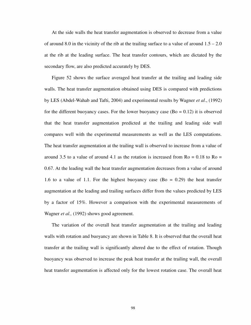
98

At the side walls the heat transfer augmentation is observed to decrease from a value

of around 8.0 in the vicinity of the rib at the trailing surface to a value of around 1.5 – 2.0

at the rib at the leading surface. The heat transfer contours, which are dictated by the

secondary flow, are also predicted accurately by DES.

Figure 52 shows the surface averaged heat transfer at the trailing and leading side

walls. The heat transfer augmentation obtained using DES is compared with predictions

by LES (Abdel-Wahab and Tafti, 2004) and experimental results by Wagner et al., (1992)

for the different buoyancy cases. For the lower buoyancy case (Bo = 0.12) it is observed

that the heat transfer augmentation predicted at the trailing and leading side wall

compares well with the experimental measurements as well as the LES computations.

The heat transfer augmentation at the trailing wall is observed to increase from a value of

around 3.5 to a value of around 4.1 as the rotation is increased from Ro = 0.18 to Ro =

0.67. At the leading wall the heat transfer augmentation decreases from a value of around

1.6 to a value of 1.1. For the highest buoyancy case (Bo = 0.29) the heat transfer

augmentation at the leading and trailing surfaces differ from the values predicted by LES

by a factor of 15%. However a comparison with the experimental measurements of

Wagner et al., (1992) shows good agreement.

The variation of the overall heat transfer augmentation at the trailing and leading

walls with rotation and buoyancy are shown in Table 8. It is observed that the overall heat

transfer at the trailing wall is significantly altered due to the effect of rotation. Though

buoyancy was observed to increase the peak heat transfer at the trailing wall, the overall

heat transfer augmentation is affected only for the lowest rotation case. The overall heat

99

transfer augmentation at the leading surface decreases with rotation. However, very little

difference is observed with the variation of buoyancy.

Ro

Nu/

Nu 0

0 0.2 0.4 0.60

1

2

3

4

5

6 Wagner Bo = 0.07 - 0.16LES, Bo = 0.12DES, Bo = 0.12

Trailing Side

Leading Side

Ro

Nu/

Nu 0

0 0.2 0.4 0.60

1

2

3

4

5

6Wagner Bo = 0.26 - 0.34LES, Bo = 0.29DES, Bo = 0.29

Trailing Side

Leading Side

Figure 52: Comparison of the surface averaged ribbed wall heat transfer augmentation

Ro

Nu/

Nu 0

0 0.2 0.4 0.61

2

3

DES, Bo = 0.12LES, Bo = 0.12

Ro

Nu/

Nu 0

0 0.2 0.4 0.61

2

3

DES, Bo = 0.29LES, Bo = 0.29

Figure 53: Comparison of the side wall heat transfer augmentations

Figure 53 shows the comparison of the side wall heat transfer as predicted by DES in

comparison with the heat transfer reported by LES studies (Abdel-Wahab et al., 2004).

The side wall heat transfer augmentation predicted by DES compares well with LES. It is

observed that the surface averaged heat transfer augmentation increases as the rotation is

increased from 0.18 to 0.35, but remains constant as the rotation is further increased to

Ro = 0.67. A slight difference is observed in the side wall heat transfer for the Ro = 0.67

100

and Bo = 0.29 between DES and LES. However the value predicted by DES, is within

7.5% of the value predicted by LES.

Table 8: Variation of the heat transfer augmentation at the ribbed and side walls for different rotation and buoyancy cases

Ro 0.18 0.35 0.67

Bo 0.00 0.12 0.29 0.00 0.12 0.29 0.00 0.12 0.29

Re 18990 18040 17950 17080 17340 17660 20040 20520 20360

Trailing 3.05 3.52 3.60 3.79 3.74 3.88 4.05 4.11 4.04

Leading 1.41 1.60 1.51 1.54 1.39 1.46 1.32 1.12 1.29

Side Wall 2.28 2.27 2.46 2.22 2.56 2.61 2.60 2.66 2.45

Table 8 shows the variation of the heat transfer augmentation at the side walls with

rotation and buoyancy. It is observed that the variation in the side wall heat transfer is not

affected much by buoyancy. Rotation also results in a smaller change in the heat transfer

as compared to the trailing wall. This behavior is in agreement with the trends observed

by Wagner et al., (1992).


Earlier studies have shown the deficiencies of the popular RANS models in

accurately predicting the effects of buoyancy in ribbed ducts as well as in several other

applications like cavity flows, atmospheric flows etc. Addition of ad hoc terms have also

proposed, but these terms have often failed to work in flows outside the flow regime for

which it was proposed. The application of DES based on an eddy-viscosity RANS model

improves the prediction capabilities considerably as no additional terms are necessary to

101

model the effects of buoyancy. The present study validates the capability of DES in

predicting the flow and heat transfer in internal cooling passages when subjected to

rotation and the effects of buoyancy are significant. Earlier LES studies (Abdel-Wahab

and Tafti, 2004) have been used for detailed comparisons of the flow and heat transfer

physics, while the surface averaged heat transfer augmentation are validated with the

experimental measurements by Wagner et al., (1992).

The comparison of the mean flow features shows that the flow stabilizes at the

leading surface as a result of which reattachment length of the flow increases as the

buoyancy is increased. Destabilization of the flow at the trailing surface results in a

shorted reattachment length. The opposite effect is observed at the leading surface.

Buoyancy also results in an increase in the turbulence at the trailing surface and decreases

at the leading surface. Heat transfer increases with buoyancy at the trailing surface. At the

leading surface the effective heat transfer area is decreased as the recirculation zone

occupies a large portion of the inter-rib space. Smaller changes are observed in the heat

transfer at the side walls.

A comparison of the detailed flow physics with LES shows that DES predicts the

primary and the secondary flow features in the duct accurately. Apart from predicting the

flow features, the augmentation and attenuation of turbulence is predicted as accurately

as an equivalent LES computation. Heat transfer distributions at the ribbed and side

walls, being functions of the mean and turbulent flow features are predicted well by DES.

The trends observed in the heat transfer augmentations at the ribbed and side walls are

also consistent with the experimental observations by Wagner et al., (1991). The overall

heat transfer augmentations predicted by DES compares well with LES and experiments.

102

In summary, it is observed that DES accurately predicts the physics of the flow

dominated by shear and buoyancy. The main contribution is in establishing the capability

of DES in predicting the effects of the extra strain generated by buoyancy. It is observed

that DES computations can be carried out at reasonable costs, almost an order of

magnitude less than the equivalent LES computation.

103

6 Flow and Heat Transfer in a complete Two Pass Duct

connected by a 180º Bend

The previous chapter validates the performance of DES in predicting the flow and

heat transfer in the fully-developed regions of the ribbed duct. The following study builds

on the studies on fully-developed ducts and focuses on the validation of DES in two-pass

ducts. In the process the capabilities of DES in predicting the development of the flow

and heat transfer in the first pass of the duct till it attains a fully developed state, the

effects of the bend in the two-pass duct and the flow and heat transfer downstream of the

bend are studied. The initial part of the study investigates the application of DES in a

stationary two-pass duct. This is followed by an investigation of the effects of rotation in

the two-pass duct.

The flow and heat transfer in a ribbed internal cooling duct is a function of the flow

Reynolds number and the geometric parameters such as the rib height to hydraulic

diameter ratio, the rib pitch, the aspect ratio of the duct, the angle of the rib with respect

to the flow and the shape of the rib as shown by previous studies (eg. Johnson et al.,

1994). Additionally, when rotation is introduced, the Coriolis forces significantly alter the

primary and secondary flow features of the flow. The Coriolis forces therefore affect the

heat transfer at the ribbed walls in both the first and the second passes of the cooling duct.

Computations are carried out for a ribbed square channel with a rib pitch to rib height

(P/e) of 10 and rib height to hydraulic diameter (e/Dh) of 0.1 for a bulk Reynolds number

of 20,000. Each rib section (block) consists of two in-line ribs placed at the center of the

channel at the top and the bottom walls. The ribs are placed normal to the flow direction

104

and have a square cross-section. Since DES is less expensive than LES, a complete

analysis of a two pass channel with 12 sets of ribs in the first and the second pass has

been carried out. The two passes are connected by a 180º bend whose width (W) is half

the hydraulic diameter (W/Dh = 0.5). The geometry used for the computation is shown in

Figure 54.

Figure 54: The two-pass internal cooling duct geometry studied

A no-slip boundary condition is imposed on the walls and the ribs. The conditions set

at the wall are 0=u

, k = 0, and 21Re/6 yβω τ→ as 0→y , which is derived from a

molecular diffusion and dissipation balance on smooth surfaces (Wilcox, 1988). The

turbulent Prandtl number is assumed to have a constant value of 0.9. A uniform laminar

inlet condition is imposed to approximate the flow exiting a plenum into the inlet section

of the duct. At the outflow, a convective condition of the form 0=∂∂+

∂∂

xc

tφφ

is applied,

105

where c is the mean convective velocity and φ is the variable being convected out (φ = ,

, k and ω).

The grid in a rib pitch consists of 65 nodes in the streamwise direction and 65 x 65 in

the cross-stream direction. The grid used for one pitch has been tested and found to be

optimal for DES (fully-developed) computations on stationary and rotating ducts

(Chapter 2.3). In total, each unit was discretized into 64 x 64 x 64 cells and was divided

into 4 equal blocks in the spanwise direction to facilitate parallel processing. The 180º

bend was discretized into 64 x 64 x 32 cells and divided into two blocks. The second leg

of the duct had an outlet region which was around 4 hydraulic diameters long. All these

sum to 7.7 x 106 cells which are distributed in 110 blocks.

A non-dimensional time step (non-dimensionalized based on the bulk velocity and the

hydraulic diameter of the duct) of 1 x 10-4 was used in all of the cases. Calculations are

initiated by assuming a uniform flow velocity in the computational domain and imposing

a uniform laminar flow inlet profile, approximating the flow exiting a plenum into the

ribbed channel. Time evolution of bulk quantities such as surface-averaged Nusselt

numbers and friction factors are monitored as the solution is allowed to reach a

statistically steady state for about 30 non-dimensional time units. The mean

characteristics of the flow are obtained by averaging the solution for an additional 10

time units.

6.1 Stationary Two-Pass Duct

In the current study, DES and URANS are carried out in a complete two-pass channel

with 12 ribs in the first and second passes, connected by a 180 degree bend. The flow in

106

the first pass of the duct is compared with LES computations by Sewall et al. (2006a).

The flow in the fully developed region is also compared with experiments by Rau et al.

(1998). The flow in the 180 degree bend is compared with LES results in the bend by

Sewall and Tafti (2006b) and experimental results by Sewall et al. (2006a). The LES

computations have been validated extensively with experiments in Sewall et al. (2006a),

and except for some differences at the center of the duct and in the 180 degree bend, all

physical phenomena characterized by mean and turbulent rms quantities are reproduced

with excellent quantitative accuracy.

Figure 55: Comparison of streamlines in the developing region through a plane passing through the center z-plane

6.1.1 Mean Flow Field

6.1.1.1 Streamwise Flow Development in First Pass

Figure 55 shows the development of the flow. The LES calculation (Sewall et al,

2006a) shows that the separated shear layer at the first set of ribs immediately transitions

to turbulence. The separation zone behind the first rib extends the whole pitch and

reattaches just upstream of the second set of ribs. However, at the second rib, because of

the increased mixing promoted by turbulence, the separated zone extends only half the rib

107

pitch, after which the flow structure quickly settles down to a near fully-developed state,

with small changes occurring in the flow structure and turbulent characteristics. The flow

quantities change in magnitude further downstream and a “near-fully-developed” state is

established by the third to fourth rib. A comparison of the streamlines injected at the inlet

shows that DES predicts that the flow separating after the first rib reattaches in the inter-

rib region after passing the second rib. At the first three ribs, the separation zones are

much larger than in LES which implies that DES is unable to predict the rapid transition

to a turbulent state. In the URANS case the first rib trips the flow and the flow transitions

immediately after the first rib. The flow reattaches between the first and the second ribs

and immediately settles down to a fully turbulent flow. This can be clearly identified in

Figure 55.

Figure 56: Comparison of u-velocities in the developing region through the center z-plane

A comparison of the streamwise velocity contours (Figure 56) shows that the DES

results are slightly different than that predicted by LES for the first three to four rib pairs.

The streamwise velocity distribution in the cross-section is less “plug-like”, but shows a

gradual increasing trend towards the center of the duct. Though differences are observed

in the reattachment lengths between the DES and LES predictions, the centerline

108

velocities predicted by LES and DES reach a constant value of 1.4 times the bulk velocity

after the first three ribs. The flow predicted by the URANS shows the immediate

transition of the flow as it passes the first rib and attains a flat turbulent profile

downstream. The magnitudes of the center line velocities observed in the URANS case is

less than the velocity magnitudes observed in LES and DES.

(a) (b)

(c) (d)

Figure 57: U-velocities at a plane passing through the rib (a) Experiments Rau et al., (1998), P/e = 9 (b) LES – Fully Developed Region (Rib 6) (c) DES – Fully Developed Region (Rib 6) (d) URANS – Fully Developed Region (Rib 6)

Figure 57 compares the flow features in the vicinity of the rib 6 (where the flow is

fully developed) predicted by DES and URANS with the flow predicted by LES (Sewall

et al., 2006a) and experiments (Rau et al., 1998). For P/e = 9, at a plane passing through

y/e = 0.15, Rau et al., (1998) observed the maximum velocity to lie at a distance of

around 0.15Dh from the wall in the fully developed region. Though some differences in

magnitude of the velocities are observed due to the different rib pitch in the experiments,

LES and DES predict this feature in the fully developed region of the first pass of the

109

duct. URANS fails to predict this offset and predicts a uniform high velocity region

spanning the channel.

Figure 58 shows the streamwise velocities measured at a plane passing through the

center at the y/e = 0.1 plane. The separated region behind the rib experiences a reverse

flow, which is evident from the negative velocities behind the rib up to the reattachment

region. The flow accelerates after reattachment and separates in front of the next rib as

shown by the small negative velocities upstream of the rib (x = 5.35). The separation in

front of the rib is predicted accurately by DES, and the velocity magnitudes are consistent

with the fully developed experimental data. URANS predicts early attachment of the flow

and also fails to predict the recirculation regions immediately upstream and downstream

of the rib.

x

u/U

0

5 5.2 5.4 5.6 5.8 6-0.4

-0.2

0

0.2

0.4Rau et al.Rib 6, DESRib 6, URANS

Figure 58: Comparison of the streamwise velocities at y/e = 0.1 with experimental data.

6.1.1.2 Development of Secondary Flows

Secondary flows in the duct cross-section have a large effect on heat transfer

augmentation on the smooth walls. Unlike skewed or angled ribs, which exhibit strong

secondary flow patterns, normal rib induced secondary flows are comparatively weak but

110

highly localized and strong near the junction of the rib with the side walls. The vortex

shedding at the junction induces strong spanwise velocities in the vicinity of the smooth

wall. This feature is difficult to predict by standard eddy-viscosity RANS models (Ooi et

al., 2002, Chapter 5.3.1).

Figure 59: Comparison of w-velocities in the developing region through a plane near the side wall

Figure 59 shows the development of the spanwise velocity contours at a plane near the

side wall (z/Dh = 0.05). LES predicts the establishment of this feature by the third rib

pair, whereas DES predicts it only after the fourth rib pair, however after it is established,

the magnitudes are consistent between the two methods. URANS, as in the earlier

computations, fails to predict the secondary flow accurately. The w-velocities predicted

by URANS are of an order of magnitude less than that predicted by DES and LES.

111

xw

/U0

5 5.2 5.4 5.6 5.8 6

-0.20

0.00

Rau et al.Rib 6, DESRib 6, URANS

Figure 60: Secondary flow in the duct measured at y/e = 1.5 and z/Dh = 0.45

The lateral w-velocities measured above the rib along a line close to the smooth side

wall (y/e = 1.5, z/Dh = 0.45), also shows very good agreement of the secondary flow

predicted by DES in the vicinity of rib 6 with the fully developed experimental results. It

is observed that there is little spanwise movement of the fluid in the region after

reattachment while in the vicinity of the ribs (x = 5.4 – 5.6) a strong secondary velocity is

observed. The k-ω model when used in the URANS mode calculates a near zero spanwise

velocity at these locations.

6.1.1.3 Heat Transfer in the First Pass

Figure 61 shows the heat transfer at the side and the ribbed walls as predicted by LES

(Sewall et al., 2006a). The secondary flows in the duct cross-section play an important

role in the side wall heat transfer. In the vicinity of the rib the secondary flow impinging

on the side walls results in high heat transfer and the heat transfer increases up to 3.5

times that in a smooth duct. On moving towards the center of the side walls the heat

transfer is observed to be close to the values obtained in a smooth channel.

112

At the ribbed walls the heat transfer augmentation on an average is observed to be

close to 2.5 in most of the regions. Heat transfer as high as 3.0-3.5 is observed

immediately upstream of the ribs, caused by the unsteady vorticies. Immediately

downstream of the rib low heat transfer is observed. The heat transfer is observed to

reach a quasi periodic state by the 4th rib. The above observations from the LES

computation are used to compare the heat transfer predicted by DES and URANS. The

initial development of heat transfer as predicted by DES is slower than the LES

computations. However by the 4th rib the heat transfer is observed to be fully developed.

The heat transfer predictions are consistent with LES, but slightly higher levels of heat

transfer are observed upstream of the ribs and in the shear layer near the smooth side

wall. URANS predicts the heat transfer at the ribbed and the smooth wall reasonably

well. However the failure to accurately predict the secondary flows results in low levels

of heat transfer augmentations in the vicinity of the rib at the side walls.

113

Figure 61: Heat transfer augmentation in the first pass of the two-pass duct at the side wall (Top) and Ribbed Wall (Bottom)

The heat transfer predictions by DES and URANS near the 6th rib, where the flow is

fully developed are compared with the heat transfer predicted by LES (Sewall et al,

2006a) and observed by experiments (Rau et al., 1998) (Figure 62). The heat transfer

contours obtained from the experiments for P/e = 9, show that the heat transfer is the

maximum in the vicinity of the rib which is due to the impingement of the localized

strong secondary flow. Heat transfer decreases on moving away from the ribs. LES

predicts similar trends with the heat transfer augmentation reaching a maximum value of

4.5 in the vicinity of the rib. DES slightly over-predicts the heat transfer in the shear layer

above the rib. The heat transfer distribution towards the center of the channel is consistent

with the earlier observations. URANS also predicts the variation reasonably well.

URANS however underpredicts the heat transfer in the shear layer of the rib as compared

to LES and DES.

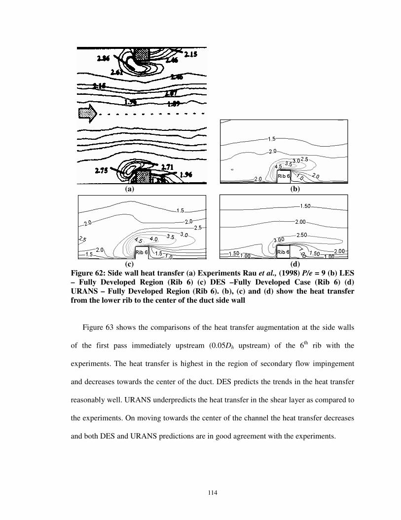
114

(a) (b)

(c) (d)

Figure 62: Side wall heat transfer (a) Experiments Rau et al., (1998) P/e = 9 (b) LES – Fully Developed Region (Rib 6) (c) DES –Fully Developed Case (Rib 6) (d) URANS – Fully Developed Region (Rib 6). (b), (c) and (d) show the heat transfer from the lower rib to the center of the duct side wall

Figure 63 shows the comparisons of the heat transfer augmentation at the side walls

of the first pass immediately upstream (0.05Dh upstream) of the 6th rib with the

experiments. The heat transfer is highest in the region of secondary flow impingement

and decreases towards the center of the duct. DES predicts the trends in the heat transfer

reasonably well. URANS underpredicts the heat transfer in the shear layer as compared to

the experiments. On moving towards the center of the channel the heat transfer decreases

and both DES and URANS predictions are in good agreement with the experiments.

115

Nu / Nu0y

1 2 30

0.1

0.2

0.3

0.4

0.5 Rau et al.Rib 6, URANSRib 6, DES

Figure 63: Comparison of side wall heat transfer with the experimental observations.

The heat transfer augmentation at the ribbed wall in the hydrodynamically and

thermally fully developed regions as predicted by DES and URANS is shown in Figure

64. These are compared with the heat transfer augmentation contours observed for P/e =

12 by Rau et al., (1998) and LES computations (Sewall et al., 2006a). A region of low

heat transfer immediately downstream of the rib is predicted, which is caused by the

presence of secondary trapped eddies. Further downstream in the primary recirculation

region, the heat transfer from the walls is gradually enhanced and reaches a maximum at

around 3.5e downstream of the rib. The point of maximum heat transfer is slightly

upstream of the reattachment, where the surface shear is a maximum. The general trends

indicate that DES is accurate in predicting the heat transfer augmentation in the

recirculation region. However, DES tends to predict an exaggerated region of high heat

transfer in front of the rib. URANS showed reasonable agreement unlike the fully

developed RANS computations (Chapter 5.3.1). Upstream of the rib the heat transfer is

under-predicted by URANS.

116

(a) (b)

(c) (d)

Figure 64: Ribbed wall heat transfer (a) Experiments Rau et al., (1998) P/e = 12 (b) LES – Fully Developed Region (Rib 6) (c) DES –Fully Developed Case (Rib 6) (d) URANS – Fully Developed Region (Rib 6). Only half of the ribbed wall is shown in (b), (c) and (d).

A comparison of the centerline heat transfer at the ribbed wall with the experiments is

shown in Figure 65. Both DES and URANS show reasonable agreement with the

experimental data. DES underpredicts and URANS overpredicts the heat transfer in the

center of the inter-rib region. A closer look at the heat transfer distribution predicted by

DES (Figure 61) shows that the higher levels of heat transfer (Nu/Nu0 > 2.50) are offset

from the center of the duct. At these locations the heat transfer is comparable to the levels

measured by the experiments. Apart from overpredicting the heat transfer downstream of

the rib, URANS also fails to capture the high heat transfer in front of the ribs and the

117

region of local high heat transfer behind the ribs occurring due to the presence of the

secondary recirculation.

x

Nu

/Nu 0

5 5.5 60

1

2

3

4 Rau et al.Rib 6, DESURANS

Figure 65: Comparison of ribbed wall heat transfer with the experimental measurements.

6.1.1.4 Flow Features in the180 degree Bend and Second Pass

Figure 66 shows streamlines at three cross-stream locations y = 0.5, 0.3 and 0.15 for

the flow entering and exiting the 180 degree bend as predicted by DES and URANS. As

the flow approaches the bend, it accelerates at the inside of the bend and separates at the

sharp edge of the bend. The separated region occupies the central 25-40% of the duct

height and its shape and extent are predicted well by DES. DES predicts a recirculating

region which does not quite sustain itself throughout the height of the duct. Further, the

flow is characterized by impingement on the back wall and outer downstream wall of the

duct which coincide with regions of high heat transfer. LES computations (Sewall and

Tafti, 2005) showed similar recirculation regions at the inner wall and the outer corners

of the bend. URANS on the other hand does not show any separation downstream of the

bend or at the inner wall of the bend. URANS also fails to predict the recirculation at the

118

outer walls of the bend. However URANS predicts a slight separation downstream of the

bend on moving down the height of the duct.

Figure 66: Comparison of the flow predicted by DES and URANS in the 180 degree bend.

Figure 67: Secondary flow at the center of the 180 degree bend. Figure 67 shows the secondary flow in the center of the bend as predicted by DES

and URANS. DES predicts Dean vortices in the vicinity of the inner and the outer walls.

119

These vortices are responsible for higher levels of heat transfer at the inner and the outer

walls of the bend. URANS also predicts one large secondary full cell in each half of the

cross-section. It is observed from the length of the velocity vectors plotted that the

secondary velocities predicted by URANS is more than that predicted by DES, especially

in the core of the bend.

To verify the accuracy of the flow predicted by URANS and DES, the streamwise

velocities computed at the center of the 180 degree bend at different locations are

compared with LDV data from Sewall et al. (Figure 68). At all y-locations, the velocity in

the outer part of the bend (x = 12.0 to 12.5) is quite uniform at approximately 1.5 times

the bulk velocity. However, at the inside of the bend, the streamwise velocity steadily

decreases as y increases with a reversal in the flow direction occurring between y=0.27

and y=0.37. The profile at y = 0.27 shows a velocity of nearly zero, indicating that the

recirculation zone occupies about 25% of the height of the duct. It is observed that in all

the locations DES predictions match well with experiments. DES comparisons are better

than URANS at these locations. URANS fails to predict the recirculating cells in the 180

degree bend, as observed in the profiles at y = 0.37 and 0.44.

120

w

X

-1 0 1 20

1

DESURANSMeasured

y= 0.02

w

X

-1 0 1 20

1

DESURANSMeasured

y= 0.27

w

X

-1 0 1 20

1

DESURANSMeasured

y= 0.37

w

X

-1 0 1 20

1

DESURANSMeasured

y= 0.44

w

X

-1 0 1 20

1

DESURANSMeasured

y= 0.02

w

X

-1 0 1 20

1

DESURANSMeasured

y= 0.27

w

X

-1 0 1 20

1

DESURANSMeasured

y= 0.37

w

X

-1 0 1 20

1

DESURANSMeasured

y= 0.44

Figure 68: Velocities in the center of the 180° bend in comparison with experiments by Sewall et al., (2006a).

6.1.1.5 Heat Transfer in the 180 degree Bend

Figure 69 shows the comparison of the heat transfer at the side and ribbed walls in the

vicinity of the 180 degree bend. The predictions are compared to LES (Sewall and Tafti,

2006b) which was performed in a geometry similar to the one used in this study with

slight differences in the flow conditions. The LES computation was initiated by

introducing a fully developed time dependent turbulent flow at the inlet which is three

hydraulic diameters upstream of the bend, while the DES and the URANS computations

have been carried out on a whole two pass channel. Another difference is that the LES

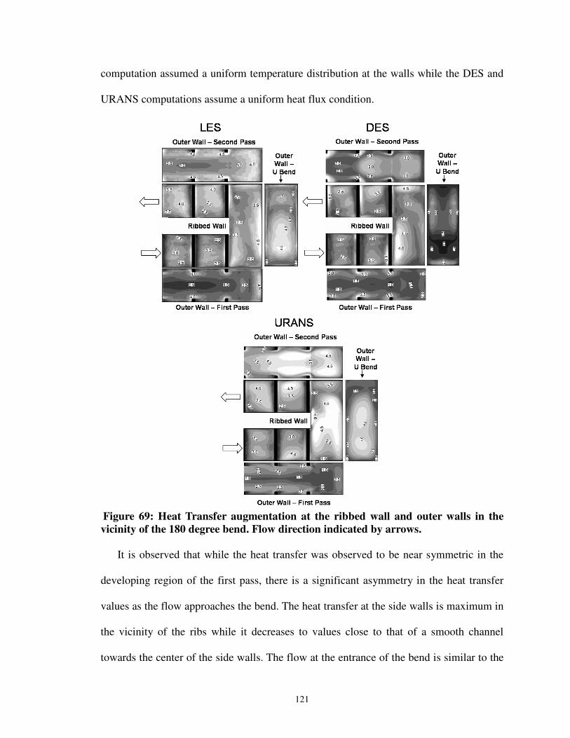
121

computation assumed a uniform temperature distribution at the walls while the DES and

URANS computations assume a uniform heat flux condition.

Figure 69: Heat Transfer augmentation at the ribbed wall and outer walls in the vicinity of the 180 degree bend. Flow direction indicated by arrows.

It is observed that while the heat transfer was observed to be near symmetric in the

developing region of the first pass, there is a significant asymmetry in the heat transfer

values as the flow approaches the bend. The heat transfer at the side walls is maximum in

the vicinity of the ribs while it decreases to values close to that of a smooth channel

towards the center of the side walls. The flow at the entrance of the bend is similar to the

122

flow around skewed ribs and so the region of high heat transfer is observed to widen as it

enters the bend. In the bend Dean vortices increase the heat transfer both at the the outer

wall. The skewness in heat transfer prevails in the second pass of the channel.

Impingement of the flow on the outer walls caused high heat transfer as the flow turns

into the bend from the first pass and into the second pass from the bend. The general heat

transfer downstream of the 180 degree bend is higher than the heat transfer upstream.

Similar observations were also made in earlier experimental studies by Ekkad et al.,

(1997), where the heat transfer profiles at the center of the ribbed wall showed the effect

of the bend on the heat transfer in the second pass.

Since the turbulence levels are predicted accurately at the ribbed walls, the heat

transfer is predicted accurately by DES. A comparison of the results shows that while the

heat transfer predicted by DES at the ribbed walls compares well with LES, the heat

transfer is underpredicted at the outer wall in the bend and in the second pass. This

underprediction may be attributed to the difference in the inlet conditions. LES

computations model the bend separately with a turbulent inlet two ribs upstream of the

bend, while DES models a developing flow from an inlet that is located 12 ribs upstream

of the bend. So the effect of flow impingement on the heat transfer is lower as predicted

by DES as compared to LES. URANS severely overpredicts the heat transfer in the bend

and downstream in the second pass, both at the ribbed walls as well as the outer walls.

6.1.1.6 Pitch Averaged Frictional Losses

Figure 70 shows the comparison of the block averaged friction factor values obtained

from DES and URANS with the LES computations (Sewall et al., 2006a, Sewall et al.,

2006a). The LES data has been collected from two cases: stationary developing flow

123

(Sewall et al., 2006a) for the first 9 ribs in the first pass, and LES computations in a 180

degree bend (Sewall et al., 2006b), for the 180 degree bend and two ribs upstream and

downstream of the bend. In the DES and URANS computations the data is obtained by

using the average pressure drop across one pitch (f = -p/2l) across a rib and the data is

fitted to a spline. Slight differences from the LES are expected in the vicinity of the 180

degree bend since the LES computation was carried out assuming a fully developed

turbulent flow two ribs upstream of the bend, while a complete channel is studied in this

case.

A comparison of the friction factors shows that DES, like LES predicts a negative

friction factor due to pressure recovery downstream of the inlet. URANS completely fails

to predict this recovery and predicts a large pressure drop across the first rib. Further

downstream as the flow reaches a fully developed state the predictions by DES as well as

URANS are consistent with the LES predictions. The average friction factor, as predicted

by DES and URANS, from the 4th rib to the 10th rib is observed to be around 8.15 times

that in a smooth channel which compares well with the LES value of 8.5.

Section #

f/f0

0 5 10 15 20 25-40

-20

0

20

40

60DESURANSLESGraham et al

FirstPass

SecondPass

Figure 70: block averaged friction factors in the complete channel

124

Section #

Nu/

Nu 0

5 10 15 20 250

1

2

3

4

DESURANSLES

First Pass Second Pass

Section #

Nu/

Nu 0

5 10 15 20 250

1

2

3

4

DESURANSLES


(a) (b)

Section #

Nu/

Nu 0

5 10 15 20 250

1

2

3

4

DESURANSLESWagner et al


(c)

Figure 71: Block averaged heat transfer at (a) inner wall (b) outer wall (c) ribbed wall

The shear induced due to the turning of the flow upstream of the 180 degree bend

results in a higher friction factor in the region. Based on the LES predictions the friction

factor immediately upstream of the bend is around three times that in a fully developed

case. The friction factor in the bend is almost of similar magnitude but as the flow turns

the corner (block 14 in Figure 1) it encounters a large drop in pressure. Pressure recovery

results in a negative friction factor immediately downstream which is similar to the entry

125

region where an initial drop in pressure is followed by a pressure recovery. The pressure

drop predicted in the vicinity of the 180 degree bend by DES compares well with the LES

cases. URANS over-predicts the friction factor in the vicinity of the bend. As the flow

settles down in the second pass, the average friction factor in the second pass of the duct

is observed to be close to 9.5 as predicted by DES and URANS.

6.1.1.7 Pitch Averaged Heat Transfer Augmentation

Figure 71 shows the comparison of the pitch averaged heat transfer predicted by the

DES and URANS with LES computations (Sewall et al., 2006a-b) at the ribbed and the

side walls. DES predictions in the first 4 ribs in the developing region of the duct are

inconsistent with LES. However after the flow is (hydrodynamically and thermally)

developed the predictions by DES are consistent with LES. URANS predictions at the

side walls in the first six blocks agree with LES predictions but the heat transfer is over-

predicted downstream in the fully developed region.

At the ribbed wall the heat transfer is under-predicted at the ribbed wall of the first 4

blocks by both DES and URANS. Further downstream in the fully developed region of

the duct the heat transfer predictions are consistent with LES predictions.

Heat transfer increases in the vicinity of the 180 degree bend at all the walls. The

DES predictions in the vicinity of the 180 degree bend are consistent with the LES

results, though the values are slightly over-predicted at the inner wall. URANS shows

little agreement with the DES and LES in the vicinity of the 180 degree bend.

In the second pass of the duct, the heat transfer at all the walls is higher than the first

pass, due to the increase in turbulence and stronger secondary flows. Experiments by

126

Liou et al., (2001) also showed a similar increase in overall heat transfer in the second

pass of the duct. The overall heat transfer at the outer wall of the second pass is observed

to be higher than the heat transfer at the inner wall, which is consistent with the trends

observed by Wagner et al., (1992) in their experiments on ducts with normal ribs.


The capability of DES and URANS in predicting the flow and heat transfer in a

complete two pass channel has been evaluated. The LES computation in the developing

region of the duct used around 8.85 x 106 cells (Sewall et al., 2006a) and 8.4 x 106 cells

were used in the LES computation in a 180 degree bend (Sewall and Tafti, 2006b). The

DES and URANS computations of the complete two pass channel were carried out by

discretizing the whole domain in to 7.7 x 106 cells. The flow and heat transfer in the fully

developed region of the duct as predicted by DES compares well with the LES

computations by Sewall and Tafti (2004), Sewall et al. (2006a) and experiments by Rau

et al. (1998). URANS manages to capture the primary flow features but fails to capture

the subtle secondary flows. The flow and heat transfer predicted by DES in the 180

degree bend are also consistent with the LES results in the bend by Sewall and Tafti

(2006b) and experimental results by Sewall et al., (2006a).

DES does not predict shear layer transition with accuracy and as a result predicts a

greater development length than LES. However, once the flow is fully developed, DES

predictions compare very well with LES and experiments. The flow predicted by

URANS shows that the first rib trips the flow and the flow immediately transitions to

turbulence. The reattachment lengths are almost constant downstream of all the

subsequent ribs.

127

From the computations performed, the following conclusions can be derived:

1. In spite of shortcomings in predicting transition correctly at the entrance to the duct,

DES predicts flow and heat transfer with good accuracy in a flow which is dominated

by separation and reattachment of shear layers, unsteady vortex induced secondary

motions, and strong streamline curvature. It reproduces the correct physics and shows

good quantitative comparisons with LES and experiments after the first 4 ribs.

URANS predicts the transition as soon as the flow is tripped by the first rib and

under-predicts the center line velocities in the developing region.

2. The average flow characteristics in the fully developed regions of the first pass are

predicted with good accuracy by the DES computations. Owing to the accurate

prediction of the main flow characteristics, the heat transfer on the ribbed wall, which

is influenced mostly by the main flow, is also predicted with reasonable accuracy. The

secondary flow is also accurately captured by the DES computations, while URANS

fails to capture the secondary flow. Since the secondary flow is captured accurately

by DES, the heat transfer enhancement predicted on the side wall is accurate in the

DES case.

3. DES captures the flow features accurately in the 180 degree bend, while URANS

completely fails to predict the recirculating cells in the inner wall and the outer

corners of the bend. URANS also overpredicts the friction factor and the heat transfer

in the bend. The flow and heat transfer predicted by DES in the bend are superior to

URANS and compare well with the experiments and the LES predictions.

128

Thereby it is shown that by a small switch in the underlying model the accuracy of

the model can be improved to be consistent with the underlying physics leading to better

prediction capability.

6.2 Rotating Two Pass Duct – Effect of Coriolis Forces

The study of flow and heat transfer in a stationary two pass duct builds on the work in

stationary fully developed ducts discussed in chapter 5.3 (stationary fully developed

computation). In a similar manner this work builds on previous work (Chapter 5.4) that

validates the performance of DES is predicting the effects of Coriolis forces on the flow

and heat transfer in the fully developed region of the internal cooling duct.

The objective of this work is to evaluate the capabilities of DES in predicting the

effects of rotation on the turbulent flow and heat transfer in a two-pass internal cooling

ribbed duct. The present results are compared with LES calculations (Sewall et al.,

2005a, 2005b) and experiments (Wagner et al., 1992, Prabhu and Vedula, 2003). Of

particular interest is the ability of DES to predict the flow development in the duct, flow

in the 180º bend and the reversal of the effects of rotation in the second pass of the duct.

The effects of rotation become prominent immediately after the inlet in the first pass

of the duct. Coriolis forces introduce an asymmetry in the flow and heat transfer and

hence the development lengths are affected. As the flow turns around the bend the effects

of the Coriolis forces at the leading and trailing walls are reversed, as a result of the

reversal in the flow direction. Comparisons are made with experiments, LES

computations and fully developed DES computations to validate the performance of DES

in predicting the effects of rotation.

129

6.2.1 Developing Flow

Figure 72 shows the comparison of the streamwise velocities at the spanwise center

of the first pass (z/Dh = 0.5) of the internal cooling passage for a duct rotated at Ro =

0.30. The effect of rotation is evident from the shift of the maximum streamwise velocity

(u/U0 = 1.40) towards the trailing side of the duct. This shift is also accompanied by the

larger regions of negative velocities (separation downstream of the rib) at the leading

surface of the duct and shorter recirculation regions at the trailing surface. The figure

shows the flow development in the first 10 ribs (out of 12 in the first pass). It is observed

that while the flow fully develops by the 3rd – 4th rib in the stationary case, the rotating

duct shows complete development of the flow only by the 8th rib.

Ro = 0.30, DES

Ro = 0.30, LES

Figure 72: Contours of streamwise velocity at the center of the duct (z/Dh = 0.5).

A comparison of the streamwise velocities predicted by DES (64 x 64 x 64 grid per

rib pitch) with analogous LES computations (96 x 96 x 96 grid per rib pitch) shows some

differences. LES and DES show similar levels of velocities in the duct. While it is

observed that while LES predicts the maximum velocity in the fully developed region of

the duct to move towards the leading wall, DES predicts the maximum velocity to move

towards the trailing wall. However the DES predictions concur with the observations

130

reported by Liou et al., (2001). LDV measurements conducted by Liou on two pass ducts

at a Reynolds number of 10,000 and rotation rates ranging from 0.0 to 0.2, showed a

maximum velocity of around 1.40 – 1.50 times the bulk velocity skewed towards the

trailing wall, as rotation is introduced in the duct.

(a)

(b) (c)

Figure 73: Comparison of the streamwise velocities at y/e = 0.15 in the fully developed regions of the flow for (a) Stationary Case (b) Ro = 0.30, Near Leading Wall (c) Ro = 0.30, Near Trailing Wall

Rau et al., (1998) studied the flow features at a plane passing through the rib located

at a distance of 0.15Dh from the ribbed wall, and observed the maximum velocity in this

plane upstream of the rib at a distance of around 0.35Dh from the centerline. DES

captures this feature in the fully-developed region accurately for the stationary, two pass

cooling duct as shown in Figure 73(a). Rotation preserves this trend as can be observed in

Figure 73(b)-(c), but the magnitudes are significantly different. The larger recirculation

region at the leading wall results in lower velocities near this wall, while the smaller

131

recirculation region at the trailing wall followed by the acceleration of the flow after

reattachment results in higher velocities near the trailing wall.

(a) (b)

Figure 74: Comparison of the secondary flow contours on top of rib 9 (a) DES (b) LES

The effect of Coriolis forces is also felt by the secondary flows. Figure 74 shows the

comparison of the secondary flow contours in the fully developed region of the duct as

predicted by DES and LES. The presence of ribs results in convergence of the flow as it

passes over the ribs and hence positive v-velocities are observed above the rib on the

trailing surface and negative velocities below the rib on the leading surface. In the

vicinity of the side wall, DES predicts an increase in the v-velocities at the trailing

surface and a decrease at the leading surface. This feature is consistent with LES

predictions. The spanwise velocities observed on top of the ribs are negligible except near

the side walls where the flow impinges on the side walls. A comparison of the secondary

velocities with LES predictions shows good agreement near the side walls. Slight

differences are observed in the v-velocities at the center of the duct, with the LES

132

predicting a strong secondary flow from the trailing wall to the center of the duct while

DES predicts a weaker flow.

6.2.2 Heat Transfer Augmentation in the First Pass

Figure 75 and Figure 76 show the heat transfer augmentation at the leading and the

trailing walls of the rotating duct as predicted by DES and LES. The heat transfer

predicted by DES is compared with the LES computations. As rotation is introduced the

heat transfer at the leading wall is observed to be lower than the heat transfer for a

stationary duct. A comparison of the heat transfer predicted by DES with LES shows that

DES underpredicts the heat transfer in the developing region of the duct. This feature is

similar to the heat transfer predictions in the stationary duct. However as the flow

develops the heat transfer levels are observed to be consistent with the LES computations

in the fully-developed regions of the duct.

(a)

(b)

Figure 75: Heat transfer augmentation for the first pass of the rotating duct at the leading wall (a) DES (b) LES

133

(a)

(b)

Figure 76: Heat transfer augmentation for the first pass of the rotating duct at the trailing wall (a) DES (b) LES

A comparison of the heat transfer predictions at the trailing surface further highlights

the deficiency. Coriolis forces augment the turbulence in the vicinity of the trailing wall.

This results in a steady increase in the heat transfer as the flow proceeds in the duct. LES

captures this effect. Although DES captures a steady increase in the heat transfer, the

levels of heat transfer are much smaller than LES. This is attributed to the inability of

DES to predict transition to turbulence accurately. Since DES predicts a delayed

transition and hence low turbulence levels the effects of Coriolis forces are weaker. So

the heat transfer augmentation predicted is much lower.

Figure 77(a)-(b) shows the heat transfer on the side walls, predicted by LES and DES.

Along the side walls, region of high heat transfer are observed in the vicinity of the rib

due to secondary flow impingement. The heat transfer steadily decreases to lower values

on moving from the trailing wall towards the leading wall. Since DES captures the

secondary flows with reasonable accuracy, the heat transfer predictions at the side wall

are consistent with the LES predictions.

134

(a)

(b)

(c) (d)

Figure 77: (a) Heat transfer augmentation for the first pass of the rotating duct at the side wall predicted by (a) LES (b) DES (c) Development of the heat transfer at the outer side wall (0.05Dh upstream of the ribs) of the internal cooling duct (d) Comparison of the fully developed heat transfer augmentations for the stationary and the rotating cases. y = 0 represents the trailing wall and y = 1 represents the leading wall

Figure 77(c) shows the development of the heat transfer at the side wall as the flow

moves from the 3rd rib to the 10th rib. The flow is observed to be thermally fully-

developed by the 9th rib, as can be observed from the similar heat transfer distributions in

the vicinity of the 9th and 10th rib. This is comparatively slower than the heat transfer

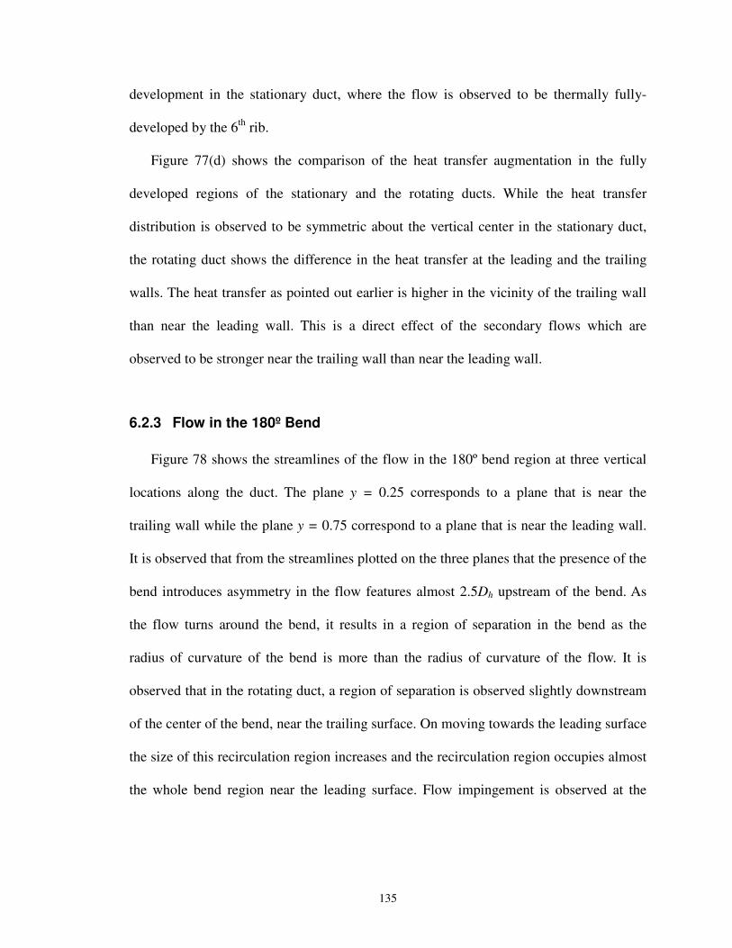
135

development in the stationary duct, where the flow is observed to be thermally fully-

developed by the 6th rib.

Figure 77(d) shows the comparison of the heat transfer augmentation in the fully

developed regions of the stationary and the rotating ducts. While the heat transfer

distribution is observed to be symmetric about the vertical center in the stationary duct,

the rotating duct shows the difference in the heat transfer at the leading and the trailing

walls. The heat transfer as pointed out earlier is higher in the vicinity of the trailing wall

than near the leading wall. This is a direct effect of the secondary flows which are

observed to be stronger near the trailing wall than near the leading wall.

6.2.3 Flow in the 180º Bend

Figure 78 shows the streamlines of the flow in the 180º bend region at three vertical

locations along the duct. The plane y = 0.25 corresponds to a plane that is near the

trailing wall while the plane y = 0.75 correspond to a plane that is near the leading wall.

It is observed that from the streamlines plotted on the three planes that the presence of the

bend introduces asymmetry in the flow features almost 2.5Dh upstream of the bend. As

the flow turns around the bend, it results in a region of separation in the bend as the

radius of curvature of the bend is more than the radius of curvature of the flow. It is

observed that in the rotating duct, a region of separation is observed slightly downstream

of the center of the bend, near the trailing surface. On moving towards the leading surface

the size of this recirculation region increases and the recirculation region occupies almost

the whole bend region near the leading surface. Flow impingement is observed at the

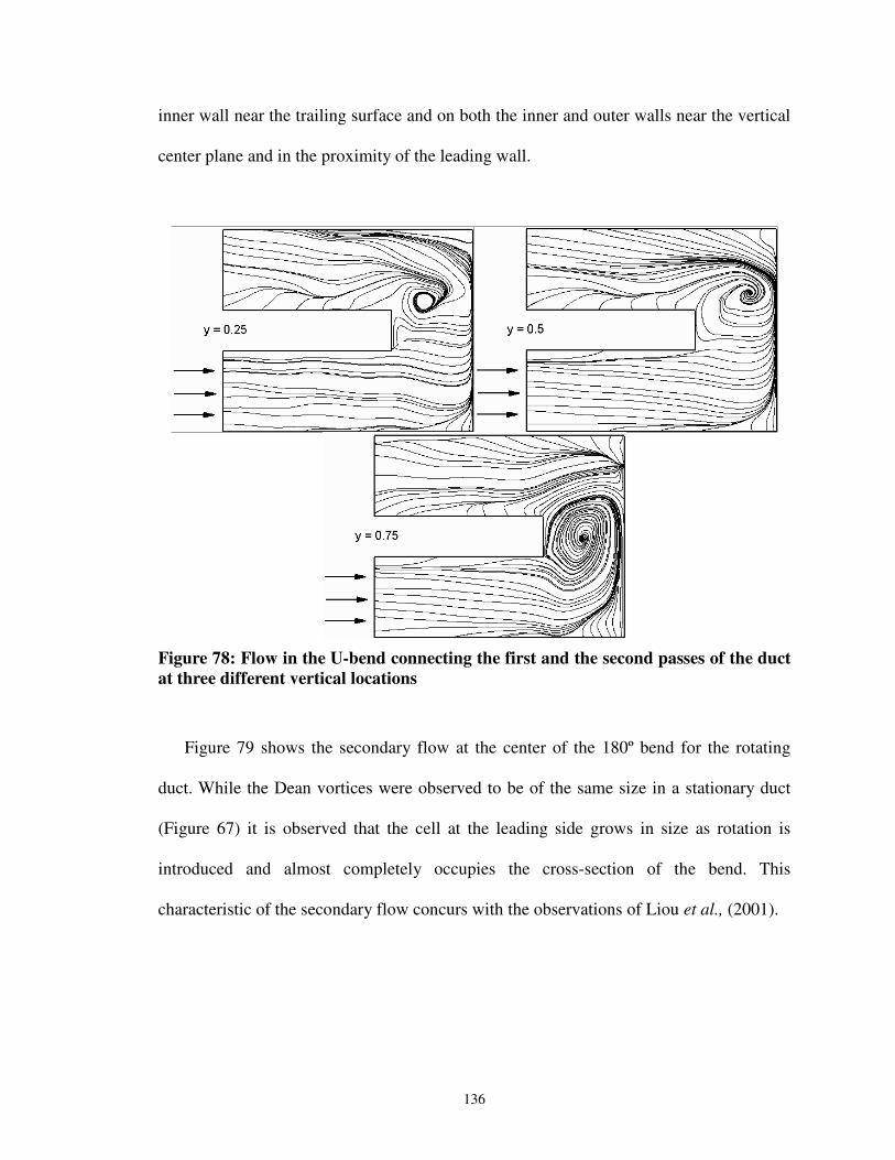
136

inner wall near the trailing surface and on both the inner and outer walls near the vertical

center plane and in the proximity of the leading wall.

Figure 78: Flow in the U-bend connecting the first and the second passes of the duct at three different vertical locations

Figure 79 shows the secondary flow at the center of the 180º bend for the rotating

duct. While the Dean vortices were observed to be of the same size in a stationary duct

(Figure 67) it is observed that the cell at the leading side grows in size as rotation is

introduced and almost completely occupies the cross-section of the bend. This

characteristic of the secondary flow concurs with the observations of Liou et al., (2001).

137

Figure 79: Secondary flow at the center of the 180º bend for the rotating duct

6.2.4 Heat Transfer in the 180º Bend

Figure 80 compares the heat transfer augmentation in the bend predicted by LES and

DES. At the leading wall it is observed that the heat transfer is low in the first pass going

into the bend. The heat transfer augmentation values of 1.4 – 2.6 predicted in this region

by DES compares well with the heat transfer predicted by LES. This value is less than the

heat transfer observed in the stationary duct. The Coriolis forces attenuate the turbulence

in the leading surface resulting in lower levels of heat transfer at this surface. As the flow

turns around the bend, higher levels of heat transfer are observed in the bend region due

to the high shear associated with the turning of the flow. DES slightly over-predicts the

heat transfer in the bend. Downstream of the bend, owing to the change in direction of the

flow, the effect of Coriolis forces are reversed resulting in augmentation of turbulence at

the leading surface. This results in high levels of heat transfer at the leading surface in the

138

second pass of the duct. The heat transfer augmentation contours predicted by DES

concur with LES.

Figure 80: Heat transfer augmentation in the vicinity of the U bend

At the trailing wall, DES underpredicts the heat transfer in the first pass of the duct,

where the flow development is observed to be slower that what was predicted by LES.

This trend is also observed in the first pass of the duct upstream of the bend. However as

the flow turns around the bend, high heat transfer is observed downstream of the last rib

in the first pass and in the vicinity of the outer wall as the flow enters and leaves the

bend. The heat transfer in the bend is slightly overpredicted by DES. The attenuation of

turbulence in the vicinity of the trailing surface in the second pass results in low levels of

139

heat transfer. The heat transfer augmentation predicted by DES agrees reasonably well

with LES in the second pass.

6.2.5 Pitch Averaged Friction Factor

The pitch-averaged friction factor reported in this study is obtained by using the

average pressure drop across the ribs (f = -p/2l). The data obtained is compared to the

fully developed DES computations and LES. The LES data is collected from two sources:

LES in a rotating developing flow in a duct (Sewall and Tafti, 2005a) for the first 9 ribs

and LES in a 180º bend for the bend and two ribs upstream and downstream of the bend.

The comparison of the pitch averaged friction factors is shown in Figure 81.

As the flow enters through the inlet, the drastic pressure drop results in a high friction

factor at the inlet. This is immediately followed by a pressure recovery resulting in a high

value of negative friction factor between the first and the second ribs. As the flow

proceeds further into the duct the friction factor settles around a value of 8.8 which

compares well with the friction factor of 8.5, obtained from a fully developed DES case

(Chapter 5.3) and LES (Sewall et al., 2006a).

As the flow turns around the 180º bend higher friction factors are observed due to the

shear induced by the turning of the flow. The friction factor immediately downstream of

the bend reaches a value almost equal to the value of friction factor at the inlet. At the

entrance to the second pass the pitch averaged friction factor behaves in a manner very

similar to that at the inlet of the first pass. Another region of pressure recovery is

observed resulting in a small negative friction following the 180º bend. A comparison of

this trend matches well with the predictions by LES (Sewall and Tafti, 2005a). The

140

pressure drop across each rib in the second pass is also observed to settle down to a value

of around 8.5 which is the value obtained in the first pass of the internal cooling passage.

Section #

f/f0

0 5 10 15 20 25-40

-20

0

20

40

60

80LESDESFully Developed

FirstPass

SecondPass

Figure 81: Comparison of the friction factor as predicted by the present computations with LES and fully developed flow predicted by DES

Prabhu and Vedula (2003) reported the pressure drop in a two pass channel by placing

taps at the leading wall and the outer wall of ducts with 90º ribs. The geometry used is

similar to the geometry currently studied. The study defined the local pressure drop and

non-dimensionalized it by the dynamic pressure. So the pressure drop was defined as

K=(PY -Pin)/(½V2), where Pin is the pressure at the inlet and PY is the local pressure

measured. Pressure taps are placed on the leading wall and the outer wall of the duct, at

locations shown in Figure 82. Results are compared with experiments at Re = 10,000, Ro

= 0.38 and the width of the bend being 0.37Dh, which compares with Re = 20,000, Ro =

0.30 and the width of the bend of 0.5Dh used in the current case.

141

Figure 82: Locations of pressure taps in the two-pass duct used for comparison with experimental data by Prabhu and Vedula (Comparison in Table 9).

Table 9: Comparison of the surface pressure drop as predicted by the current computation in comparison with the experimental measurements by Prabhu and Vedula (2003) for the rotating duct.

Across the first

10 Ribs Across the 180º

Bend Across the last

10 ribs Leading Wall –

Prabhu and Vedula -2.00 -2.00 -1.50

Leading Wall - Current Study -2.35 -1.98 -1.47

Outer Wall – Prabhu and Vedula -2.50 -1.25 -1.50

Outer Wall - Current Study -2.40 -1.66 -1.40

A comparison of the pressure drop (K) measured in the first pass, the 180º bend and

the second pass is shown in Table 9. It is observed that the pressure drop predicted

compare well with the experimentally measured values. Differences are observed in the

value of K measured across the first 10 ribs at the leading wall which may be a result of

the slight difference in the rotation rates. The pressure drop across the bend measured

from the taps placed at the outer wall may be attributed to the difference in the bend

142

width which affects the impingement at the outer walls, thereby affecting the local

pressure at the location.

6.2.6 Rib Averaged Heat Transfer Augmentation

Section #

Nu/

Nu 0

5 10 15 20 250

1

2

3

4

5

6DESLESWagner et alFully Developed


Figure 83: Ribbed averaged heat transfer at the leading wall

The rib averaged heat transfer at the leading wall is shown in Figure 83. The values

obtained from the DES computation are compared with LES (Sewall and Tafti, 2005a),

the fully developed DES computations (Chapter 5.4) and experimental measurements by

Wagner et al., (1992). As observed in the stationary case, DES underpredicts the heat

transfer in the developing region of the duct. By the 7th rib, the rib-averaged heat transfer

settles down to a value of around 1.2 which agrees with the values predicted by LES.

This value is however slightly lower than the values predicted by the fully developed

computations and the experimental measurements. As the flow approaches the bend the

heat transfer increases due to the high shear associated with the turning of the flow. This

results in higher heat transfer in the bend. The average heat transfer at the leading wall in

the bend agrees well with LES and the experimental measurements. Downstream of the

143

bend, the Coriolis forces aid in increasing the heat transfer. This causes higher heat

transfer at the leading surface. The rib averaged heat transfer in the second pass of the

duct agrees reasonably well with the experimental measurements.

Section #

Nu/

Nu 0

5 10 15 20 250

1

2

3

4

5

6DESLESWagner et alFully Developed


Figure 84: Ribbed averaged heat transfer at the trailing wall

The rib-averaged heat transfer at the trailing wall is shown in Figure 84. As explained

in the earlier section the underprediction of heat transfer is attributed to the inability of

DES to predict transition to turbulence. Though the heat transfer augmentation increases,

the delay in development of turbulence results in an underprediction of the heat transfer

by approximately 30%. Downstream of the bend, the heat transfer at the trailing surface

decreases due to the reversal in the effects of the Coriolis forces. The trend is predicted

well by DES showing good quantative agreement with LES and experiments.


In this part of the study the predictive capability of DES in the developing flow of a

rotating ribbed duct is investigated. The internal cooling duct is subjected to rotation

about the spanwise axis, with a constant rotation rate of Ro = 0.30. The results obtained

144

from a 7.7 x 106 grid used for DES are compared to the experimental measurements, two

LES computations carried out a development region of the passage (8.85 x 106 cells) and

in the 180º bend (8.4 x 106 cells) and some fully developed DES computations.

DES predicts a delayed transition and low turbulence in the developing region of the

duct. Low turbulence levels due to delay in transition are also observed in the stationary

duct, but this effect is intensified as rotation is introduced. The cumulative effect of the

delay in transition and rotation results in an underprediction of the heat transfer. However

as the flow passes through the 180 degree bend it picks up enough turbulence resulting in

a reasonable prediction of the heat transfer augmentation in the bend. As the flow

changes direction after passing through the bend the effects of Coriolis forces are

reversed. The heat transfer augmentation increases at the leading surface and decreases at

the trailing surface. The levels of heat transfer predicted in the duct downstream of the

bend in the second pass show good agreement with LES and the measurements.

While DES is observed to combine the merits of high fidelity LES (accuracy) and

(U)RANS (low computational cost), some deficiencies still exist. One deficiency that has

been highlighted from these studies is the inability of DES to capture the transition to

turbulence accurately, which still persists as with the RANS model on which it is based.

Once the flow passes this hurdle, the flow features and heat transfer downstream in the

fully turbulent regions of the flow are predicted accurately. The transition region is

significant at the Reynolds number considered in the current computations. However, if

the Reynolds number is increased the transition region decreases in size and so the

prediction capabilities of DES are expected to be more beneficial at higher Reynolds

numbers.

145

7 Summary and Conclusions

This study investigates the performance of Detached Eddy Simulation (DES) in

predicting the non-canonical flow and heat transfer in ribbed ducts with direct

applications to the internal cooling of turbine blades. In a series of calculations it is

shown that DES successfully predicts the physics of rotation induced Coriolis forces and

centrifugal buoyancy introduced due to thermal gradients in this industry specific internal

flow configuration. The capabilities of DES in predicting the complex turbulent physics

is highlighted by studies in flow in sudden expansion ducts subjected to rotation, the flow

in a cavity with a heated wall and flow and heat transfer in stationary and rotating internal

cooling ribbed ducts. From these studies the following conclusions are reached:

1. DES performs much better than an equivalent URANS in predicting the dynamics of

separation and reattachment and in capturing the secondary flows which affect the

heat transfer

2. DES maintains a LES like accuracy at around one-tenth the computational cost.

3. The main contribution of this work is showing that DES can be successfully applied

to flows which are dominated by rotation induced Coriolis forces and centrifugal

buoyancy. While linear eddy-viscosity models exhibit severe inadequacies in

predicting such flows when used in URANS mode, DES by allowing LES like

resolution of the large scales allows itself to be receptive to secondary strain which

the base RANS model fails to capture.

7.1 Recommendations

DES is a simple, non-zonal approach for solving complex flows and has had

qualitative success over a wide range of flows. DES is also observed to provide sufficient

146

unsteady information in the resolved range. The performance of DES is superior to

URANS in several flows and demands computational power much less than LES.

In spite of these advantages, successful application of DES to a wide range of flows

poses several challenges. Some potential areas of improvement for DES are discussed.

1. DES is a strategy that depends on the grid not only for accurately resolving the

turbulence in the regions of interest, but also in determining the switch between

RANS and LES. Though guidelines have been prescribed for Spalart – Allmaras (SA)

based DES (Spalart, 2001) for external flows; grid generation is not trivial and

requires some a-priori knowledge of the flow. One probable alternative is the Scale

Adaptive Simulation (SAS) approach suggested by Menter (2003, 2005) that

compares a von Karman length scale to the turbulent length scales to determine the

switch from RANS to LES. This approach is still in its incipient stage of development

and the prediction capability of this model for a wider range of flows in the context of

two equation models remains to be established.

2. Though it is hypothesized that DES reduces to a well resolved LES solution as the

grid is refined, this reduction is not smooth. Refining the grid in the vicinity of the

wall results in the activation of the LES mode. If the grid in this region is not

sufficiently resolved to capture the dominant frequencies, the quality of the solution

deteriorates. However, local grid adaptation results in treating the regions of interest

using LES and maintaining the RANS characteristics near the wall. The effects of

local grid adaptation in resolving the unsteadiness has been shown in earlier studies

(Forsythe et al., 2002). The adaptation strategies however are empirical and are

dependent on the user’s grid generation skills.

147

3. While applying RANS characteristic in the boundary layer is advantageous in terms

of the grid requirements, DES still depends on the base RANS model to predict the

separation point. Studies on flows around circular and square cross-section cylinders

(Squires et al., 2002) have shown the capabilities of SA-DES in accurately predicting

separation in such flows. However the same feature is yet to be established using the

other DES models, especially for smooth geometries.

4. Another bottleneck for DES, as pointed out by this study its inability in predicting

transition in the separated shear layers in the rib. Accurate prediction of transition

requires a good turbulence model that can also capture transition. While incorporation

of transition models has been studied for RANS models, applying these models in

DES remains a potential area for development.

5. The transition from URANS to LES still remains a ‘grey area’ in DES (Spalart,

2001). The physics behind the switch from a completely modeled solution in the

RANS regions to a well resolved LES still remains to be understood.

148

References Chapter 1: Introduction Constantinescu, G., Squires, K. D., 2000, LES and DES investigations of turbulent flow over a sphere. AIAA-2000-0540, 2000. Constantinescu, G.S., Pacheco, R., Squires, K.D., 2002, Detached-eddy simulation of flow over a sphere, AIAA Paper 2002-0425, 2002. Forsythe, J.R., Squires, K.D., Wurtzler, K.E., Spalart, P.R., 2002, Detached-Eddy Simulation of fighter aircraft at high alpha, AIAA Paper 2002-0591, 2002. Kapadia, S., Roy, S., Vallero, M., Wurtzler, K.E., Forsythe, J.R., 2003, Detached Eddy Simulation Over a Reference Ahmed Car Model, AIAA 2003-0857, 2003. Kotapati-Apparao, R.B., Squires, K.D., Forsythe, J.R., 2003, Prediction of a prolate spheroid undergoing a pitchup maneuver, AIAA Paper 2003-0269, 2003. Morton, S.A., Steenman, M.B., Cummings, R.M., Forsythe, J.R., 2003, DES grid resolution issues for vertical flows on a delta wing and an F-18C, AIAA Paper 2003-1103, 2003. Nikitin, N.V., Nicoud, F., Wasistho, B., Squires, K.D., Spalart, P.R., 2000, An approach to wall modeling in Large-Eddy Simulation, Physics of Fluids, 12(7), pp. 1629-1632, 2000. Pope, S.B., 2001, Turbulent Flows, Cambridge University Press Shur, M., Spalart, P.R., Strelets, P.R., Travin, A., 1999, Detached-eddy Simulation of an airfoil at high angle of attack. 4th Int. Symposium on Eng. Turb. Modelling and Experiments, May 24-26 1999, Corsica. W. Rodi and D. Laurence Eds., Elsevier

Spalart, P.R., Jou, W.H., Streletes. M., Allmaras. S.R., 1997, Comments on the feasibility of LES for wings and a hybrid RANS/LES approach, First AFSOR Int. Conf. on DNS/LES, Aug 4-8, 1997, In Advances in DNS/LES, C.Liu and Z.Liu Eds, Greyden Press, Columbus, OH.

Squires, K.D., Forsythe, J.R., Morton, S.A., Blake, D.C., Serrano, M., Wurtzler, K.E., Strang, W.E. , Tomaro, R.F., Spalart, P.R., 2002, Analysis of full aircraft with massive separation using Detached-Eddy Simulation, Proceedings of the High Performance Computing Modernization Program 2002 Users Group Conference, Austin, Texas, 2002.

Strelets, M., 2001, Detached Eddy Simulation of Massively Separated Flows, AIAA 2001-0879.

Travin, A., Shur, M. L., Strelets, M., and Spalart, P.R., 2000, Detached Eddy Simulation Past a Circular Cylinder, Flows, Turbulence, and Combustion, Vol. 63, pp. 193-313, 2000. Viswanathan, A.K., Squires, K.D., Klismith, K., Forsythe, J.R., 2003, Detached-Eddy Simulation around a forebody at high angle of attack, AIAA Paper 2003-0263, 2003

149

Chapter 2: Literature Review Abdel-Wahab, S., Tafti, D. K., 2004b. Large Eddy Simulations of Flow and Heat Transfer in a 90º Ribbed Duct with Rotation - Effect of Coriolis and Centrifugal Buoyancy Forces, J. Turbomachinery, 126(4), pp. 627-636, 2004.GT2004-53799, ASME Turbo Expo: 2004, Vienna, Austria. Amano, R.S., Goel, P., 1995. Computation of turbulent flow beyond backward steps using Reynolds Stress closure, AIAA J, 1995 23, pp 1356. Baldwin, B. S. and Lomax, H. (1978), Thin Layer Approximation and Algebraic Model for Separated Turbulent Flows, AIAA Paper 78-257 Bo, T., Iacovides, H., Launder, B.E., 1995, Developing Buoyancy-Modified Turbulent Flow in Ducts Rotating in Orthogonal Mode, Transactions of ASME 177, pp.474-484. Bradshaw, P., 1969, The Analogy Between Streamline Curvature and Buoyancy in Turbulent Shear Flow, J. Fluid Mech, 36, Part 1, pp 177-191. Bradshaw, P., 1988, Effects of Extra Strain – Review, Near Wall Turbulence, Zoran Zaric Memorial Conference Ed. S J Kline, N.H. Afghan, Hemisphere Publishing Corporation, pp 106 - 122. Chima, R.V., 1996, A k- turbulence model for quasi-three dimensional turbo machinery flows, AIAA 96-0258. Driver, D., Seegmiller, H.L., 1985. Features of reattaching turbulent shear layer in divergent channel flow, AIAA J., 23, 162-171. Hanjalic, K., Launder, B.E., 1980, Sensitizing the Dissipation Equation to Irrotational Strains, ASME J. Fluids Eng., 102: 34. Hanjalic, K., Kenjeres, S., Durst, F., 1996, Natural convection in partitioned two-dimensional enclosures at higher Rayleigh numbers, Int. J. Heat and Mass Transfer, 39(7), pp 1407-1427. Hanjalic, K., Kenjeres, S., 2001, T-RANS simulation of Deterministic eddy structure driven thermal buoyancy and Lorentz force, Flow, Turbulence and Combustion, 66, pp 427-451. Hellsten, A., 1998, Some improvements in Menter’s k- SST turbulence model, AIAA 98-2554. Howard, J.H.G., Patankar, S.V., Bordynuik, R.M., 1980, Flow prediction in rotating ducts using Coriolis-modified turbulence models, ASME Journal of Fluids Engg, 102, pp 456-461. Humphrey, J.A.C., To, W.M., 1986, Numerical simulation of buoyant turbulent flow II – Free and mixed convection in a heated cavity, Int. J. Heat and Mass Transfer, 29(4), pp 593-610. Iacovides, H., Launder, B.E., 1991, Parametric and Numerical Study of Fully Developed Flow and Heat Transfer in Rotating Rectangular Ducts, J. Turbomachinery 133, pp.331-338. Iacovides, H., Raisee, M., 1999. Recent Progress in the Computation of Flow and Heat Transfer in Internal Cooling Passages of Turbine Blades Int. J. Heat Fluid Flow, 20. pp. 320-328, 1999. Ishigaki, H., 1996, Analogy between turbulence flows in curved pipes and orthogonally rotating pipes, Journal of Fluid Mechanics, 307, pp 1 – 10. Jia, R., Saidi, A., Sunden, B., 2002. Heat Transfer Enhancements in Square Ducts with V-Shaped Ribs of Various Angles, Proc ASME Turbo Expo, GT 2002-30209.

150

Kantha, L.H., 2004, The length scale equation in turbulence models, Nonlinear processes in Geophysics, 11, pp 83-97. Launder, B.E., Priddin, C.H., Sharma, B.I., 1977, The calculation of turbulent boundary layers on spinning and curved surfaces, ASME Journal of Fluids Engg, pp 231-239, March. Lin, Y.L., Shih, T,I-P, Stephens, M.A., Chyu, M.K., 2001, A numerical study of flow and heat transfer in a smooth and a ribbed U-duct with and without rotation, ASME Journal of Heat Transfer, 123, pp 219-232. Mellor, G. L., Yamada, T., 1982, Development of a turbulence closure model for geophysical fluid problems, Rev. Geophys. and Space Phys., 20(4), 851-875, 1982. Menter, F.R., 1993, Zonal Two Equation k- Turbulence Models for Aerodynamic Flows, AIAA Paper 93-2906. Murata, A., Mochizuki, S., 2001, Large Eddy simulation with a dynamic subgrid-scale model of turbulent heat transfer in an orthogonally rotating rectangular duct with transverse rib turbulators, Int. J. Heat Mass Transfer 43, pp. 1243-1259. Ooi, A., Iaccarino, G., Durbin, P.A., Behnia, 2002. M., Reynolds Averaged Simulation of Flow and Heat Transfer in Ribbed Ducts, Int. J. Heat and Fluid Flow, 23, pp 750-757. Peng, S-H., Davidson, L., 1999, Computation of turbulent buoyant flows in enclosures with low-Reynolds number k-ω models, Int. J Heat and Fluid Flow, 20, pp 172-184. Plett, E.G., Soultogiannis, A.A., Jouini, D.B., 1995, Numerical Simulation of ventilation air movement in partitioned offices, Indoor Air, 3, pp 26-33. Prakash, C., Zerkle, R., 1995. Prediction of Turbulent Flow and Heat Transfer in a Ribbed Rectangular Duct With and Without Rotation, ASME J. of Turbomachinery, Vol 117, pp 255-264. Rigby, D.L., 1998, Prediction of Heat and Mass Transfer in a Rotating Ribbed Coolant Passage with a 180 Degree Turn, 98-GT-329, International Gas Turbine and Aeroengine Congress and Exhibition, Stockholm, Sweden, June 2-5. Rodi., 1980, Turbulence models and their applications in hydraulics, a state of art review, Int Association of Hydraulic Research, Delft, p30. Rodi, W., Scheuerer, G., 1983, Calculation of curved shear layers with two-equation turbulence models, Physics of Fluids, 26(6). Saidi, A., Sunden, B., 2001. On Prediction of Thermal-Hydraulic Characteristics of Square-Sectioned Ribbed Cooling Ducts, ASME J. of Turbomachinery, Vol 123. Sewall, E.A., Tafti, D.K., 2005, Large Eddy Simulation of Flow and Heat Transfer in the Developing Flow Region of a Rotating Gas Turbine Blade Internal Cooling Duct with Coriolis and Buoyancy Forces, GT 2005-68519, ASME Turbo Expo 2005, June 6-9, 2005, Reno-Tahoe, Nevada, USA. Shankar, V., Davidson, L., Olsson, E., 1995, Numerical investigation of turbulent plumes in both ambient and stratified surroundings, Indoor Air, 5, pp 136-146. Sharif, M.A.R., Liu, W., 2003, Numerical study of turbulent natural convection in a side-heated square cavity at various angles of inclination, Numerical Heat Transfer, Part A, 43: 693-716.

151

Stips, A., Burchars, H., Bolding, K., 2002, Modeling of convective turbulence with a two-equation k- turbulence closure scheme, Ocean Dynamics, 52, 153-168. Strelets, M., 2001, Detached Eddy Simulation of Massively Separated Flows, AIAA 2001-0879. Tafti, D.K., 2005, Evaluating the Role of Subgrid Stress Modelling in a Ribbed Duct for the Internal Cooling of Turbine Blades, Int. J Heat and Fluid Flow 26(1), pp. 92-104. To, W.M., Humphrey, J.A.C., 1986, Numerical simulation of buoyant turbulent flow I – Free convection along a heated, vertical flat plate, Int. J. Heat and Mass Transfer, 29(4), pp 573-592. Umlauf, L., Burchard, H., Hutter, K., 2003, Extending the k-ω turbulence model towards oceanic applications, Ocean Modelling, 5, pp 195-218 Watanabe, K., Takahashi, T., 2002, LES Simulation and Experimental Measurement of Fully Developed Ribbed Channel Flow and Heat Transfer, Proc. ASME Turbo Expo: 2002-GT-30203. Wilcox, D.C., Chambers, T.L., 1977, Streamline curvature effects on turbulent boundary layers, AIAA Journal, Vol 15, No.4. Wilcox, D.C., 1988. Reassessment of the Scale-Determining Equation for Advanced Turbulence Models, AIAA Journal, Vol 26 (11), pp 1299-1310. Nov 1988. Yeoh, G.H., Yuen, R.K.K., Chen, D.H., Kwok, W.K., 2002, Combustion and heat transfer in compartment fires, Numerical Heat Transfer, Part A, 42, pp 153 – 172. Yokosawa, H., Fujita, H., Iwata, S., 1989, Measurement of Turbulent Flow in a Square Duct with Roughened Walls on Two Opposite Sides, Int. J. of Heat and Fluid Flow, Vol 10(2), pp 125-135, 1989. Zhao, C.Y., So, R.M.C., Gatski, T.B., 2001, Turbulence modeling effects on the prediction of equilibrium states of buoyant shear flows, Theoretical and Computational Fluid Dynamics, 14, pp 399-422. Chapter 3: Computational Model and Governing Equations Abdel-Wahab, S, Tafti, D.K., 2004a. Large Eddy Simulation of Flow and Heat Transfer in a Staggered 45° Ribbed Duct, ASME Turbo Expo: 2004, Vienna, Austria, GT2004-53800. Abdel-Wahab, S., Tafti, D. K., 2004b. Large Eddy Simulations of Flow and Heat Transfer in a 90º Ribbed Duct with Rotation - Effect of Coriolis and Centrifugal Buoyancy Forces, J. Turbomachinery, 126(4), pp. 627-636, 2004.GT2004-53799, ASME Turbo Expo: 2004, Vienna, Austria. Incropera, F.P. and Dewitt, 2002. D.P., Fundamentals of Heat and Mass Transfer, fifth edition, John Wiley and Sons, New York. Menter, F.R., 1992, Improved Two-Equation k- Turbulence Models for Aerodynamic Flows, NASA Technical Memorandum 103975. Menter, F.R., 1993, Zonal Two Equation k- Turbulence Models for Aerodynamic Flows, AIAA Paper 93-2906. Sewall, E.A., Tafti, D.K., Graham, A., Thole, K.A., 2005c. Experimental Validation of Large Eddy Simulation of flow and heat transfer in a Stationary Ribbed Duct. Submitted Int. J. Heat and Fluid Flow, 2005.

152

Spalart, P.R., Jou, W.H., Streletes. M., Allmaras. S.R., 1997, Comments on the feasibility of LES for wings and a hybrid RANS/LES approach, First AFSOR Int. Conf. on DNS/LES, Aug 4-8, 1997, In Advances in DNS/LES, C.Liu and Z.Liu Eds, Greyden Press, Columbus, OH. Strelets, M., 2001, Detached Eddy Simulation of Massively Separated Flows, AIAA 2001-0879. Tafti, D.K., 2001, GenIDLEST – A Scalable Parallel Computational Tool for Simulating Complex Turbulent Flows, Proc. ASME Fluids Engineering Division, FED – Vol. 256, ASME-IMECE, New York. Tafti, D.K., 2005, Evaluating the Role of Subgrid Stress Modelling in a Ribbed Duct for the Internal Wilcox, D.C., 1988. Reassessment of the Scale-Determining Equation for Advanced Turbulence Models, AIAA Journal, Vol 26 (11), pp 1299-1310. Nov 1988. Chapter 4: Validation Cases Bradshaw, P., 1969, The Analogy Between Streamline Curvature and Buoyancy in Turbulent Shear Flow, J. Fluid Mech, 36, Part 1, pp 177-191. Bradshaw, P., 1988, Effects of Extra Strain – Review, Near Wall Turbulence, Zoran Zaric Memorial Conference Ed. S J Kline, N.H. Afghan, Hemisphere Publishing Corporation, pp 106 - 122. Chong, M.S., Perry, A.E., Cantwell, B.J., 1990, A General Classification of Three-Dimensional Flow Fields, Physics of Fluids A, Vol 2 (5), pp 765-777. Chow, W.K., Gao, P.Z., 2004, Large Eddy Simulation of Turbulent Convective Cavity Flow, Int. J. Computational Fluid Dynamics, 18(8), pp 641 – 650. Ghosal, S., Lund, T.S., Moin, P., Akselvoll, K., 1995, A Dynamic Localization Model for Large Eddy Simulation of Turbulent Flows, Journal of Fluid Mechanics, Vol 286, pp 229-255. Grand, D., 1975, Contribution a l’etude des courant de recirculation, PhD. Thesis, L’Universite Scientifique et Medicale et Institut Nationale, Polytechnique, Grenoble. Hanjalic, K., Kenjeres, S., Durst, F.,1996 Natural convection in partitioned two-dimensional enclosures at higher Rayleigh numbers, Int. J. Heat and Mass Transfer, 39(7), pp 1407-1427. Hassid, S., 2002, Effects of buoyancy on the turbulence model equations., Ocean Dynamics, 52, pp 169-178. Hellsten, A., 1998, Some improvements in Menter’s k- SST turbulence model, AIAA 98-2554. Iaccarino, G., Ooi, A., Pettersson Rief, B.A., Durbin, P., 1999, RANS Simulations of Rotating Flows, Center of Turbulence Research, Annual Research Briefs, pp 257 – 266. Ideriah, F.J.K., 1980, Prediction of Turbulent Cavity Flow Driven By Buoyancy and Shear, Journal of Mechanical Engineering Science, 22(6), pp 287 – 295 Johnston, J.P.; Halleen, R.M.; Lezius, D.K., 1972, Effects of spanwise rotation on the structure of two-dimensional fully developed turbulent channel flow, J. Fluid Mech. 56, pp 533 – 557. Koutsourakis, N., Vlachogiannis, D., Sfetsos, A., Bartzis, J.G., 2003, CFD in atmospheric dispersion problems – State of the art, QNET-CFD Network Newsletter, Vol 2, No 1. Launder, B.E., Priddin, C.H., Sharma, B.I., 1977, The calculation of turbulent boundary layers on spinning and curved surfaces, ASME Journal of Fluids Engg, pp 231-239.

153

Moore, J.A., 1973, Wake and an Eddy in a Rotating, Radial-Flow Passage. Part 1: Experimental Observations, ASME Journal of Engg. For Power, pp 205 – 212. Murakami, S., Ohira, N., Kato, S., 1999, CFD analysis of a thermal plume and the indoor air flow using k- models with buoyancy effects, Flow, Turbulence and Combustion, 63, pp 113-134. Nilsen, P.J., Andersson, H.I., 1990, Rotational Effects on Sudden-Expansion Flows, Engineering Turbulence Modelling and Experiments, Elsevier Science Publications Co., Inc Rodi and Gani , pp 65-72. Peng, S-H., Davidson, L., 1999, Computation of turbulent buoyant flows in enclosures with low-Reynolds number k-ω models, Int. J Heat and Fluid Flow, 20, pp 172-184. Plett, E.G., Soultogiannis, A.A., Jouini, D.B., 1995, Numerical Simulation of ventilation air movement in partitioned offices, Indoor Air, 3, pp 26-33. Rodi, W., Scheuerer, G., 1983, Calculation of curved shear layers with two-equation turbulence models, Physics of Fluids, 26(6). Rothe, P. H.., 1975, The effects of System Rotation on Separation, Reattachment and Performance in Two-dimensional Diffusers. Stanford University Dissertation, Dept. Mechanical Engineering Rothe, P. H., Johnston, J. P., 1976, Effects of System Rotation on the Performance of Two-Dimensional Diffusers, ASME J. Fluids Eng., 9, pp. 422–430. Rothe, P.H., Johnston, J.P., 1979, Free Shear Layer Behavior in Rotating Systems, ASME J. Fluids Eng., 101, pp 117-120. Stips, A., Burchars, H., Bolding, K., 2003, Modeling of convective turbulence with a two-equation k- turbulence closure scheme, Ocean Dynamics, 52, 153-168. Wilcox, D.C., 1988. Reassessment of the Scale-Determining Equation for Advanced Turbulence Models, AIAA Journal, Vol 26 (11), pp 1299-1310. Wilcox, D.C., Chambers, T.L., 1977, Streamline curvature effects on turbulent boundary layers, AIAA Journal, Vol 15, No.4. Yeoh, G.H., Yuen, R.K.K., Chen, D.H., Kwok, W.K., 2002, Combustion and heat transfer in compartment fires, Numerical Heat Transfer, Part A, 42, pp 153 – 172. Chapter 5: Fully Developed Cases Abdel-Wahab, S., Tafti, D. K., 2004, Large Eddy Simulations of Flow and Heat Transfer in a 90º Ribbed Duct with Rotation - Effect of Coriolis and Centrifugal Buoyancy Forces, J. Turbomachinery 126(4), pp. 627-636. Chong, M.S., Perry, A.E., Cantwell, B.J., 1990, A general classification of three-dimensional flow fields, Phy. Fluids A., 2(5), pp 765 – 777. Forsythe. J.R, Squires. K.D, Wurtzler. K.E., Spalart. P.R, 2002, Detached-Eddy Simulation of Fighter Aircraft at High Alpha, AIAA Paper 2002-0591. Halleen, R.M., and Johnston, J.P., 1967, The Influence of Rotation of Flow in a Long Rectangular Channel – An Experimental Study, Report MD-18, Thermosciences Division, Dept. of Mech. Eng., Stanford University.

154

Lezius, D.K., and Johnston, J.P., 1976, Roll-Cell Instabilities in Rotating Laminar and Turbulent Channel Flows, J. Fluid Mech. Vol. 77, Part 1, pp. 153-175. Lin, Y.L., Shih, T,I-P, Stephens, M.A., Chyu, M.K., 2001, A numerical study of flow and heat transfer in a smooth and a ribbed U-duct with and without rotation, ASME Journal of Heat Transfer, 123, pp 219-232. Liou, T.M., Wu, Y.Y., Chang, Y., 1993, LDV Measurements of Periodic Fully Developed Main and Secondary Flows in a Channel with Rib-disturbed Walls, ASME Journal of Fluids Engineering, Vol 115, pp 109-114. Liou, T.M., Chen, M.Y., Tsai, M.H., 2001, Fluid Flow and Heat Transfer in a Rotating Two-Pass Square Duct with In-Line 90° Ribs, ASME Turbo Expo: 2001-GT-0185. Murata, A., Mochizuki, S., 1999, Effect of cross-sectional aspect ratio on turbulent heat transfer in an orthogonally rotating rectangular smooth duct, Int. J. Heat Mass Transfer 42, pp. 3803-3814. Murata, A., Mochizuki, S., 2000, Large Eddy simulation with a dynamic subgrid-scale model of turbulent heat transfer in an orthogonally rotating rectangular duct with transverse rib turbulators, Int. J. Heat Mass Transfer 43, pp. 1243-1259. Murata, A., Mochizuki, S., 2001, Comparison between Laminar and Turbulent Heat Transfer in Stationary Square Ducts with Transverse or Angled Rib Turbulators, 2001, Int. J. Heat Mass Transfer, 44, pp 1127-1141. Ooi, A., Iaccarino, G., Durbin, P.A., Behnia, M., 2002, Reynolds Averaged Simulation of Flow and Heat Transfer in Ribbed Ducts, 2002, Int. J. Heat and Fluid Flow, 23, pp 750-757.. Parsons, J.A., Han, J.C., Zang, Y.M., 1994, Wall Heating Effect on Local Heat Transfer in a Rotating Two-Pass Square Channel with 90º Rib Turbulators, Int. J. Heat Mass Transfer 37, 1411-1420. Prakash, C., Zerkle, R., 1995, Prediction of Turbulent Flow and Heat Transfer in a Ribbed Rectangular Duct with and without Rotation, J. Turbomachinery, 117, pp.255-264. Rau, G., Cakan, M., Moeller, D., Arts, T., 1988, The Effect of Periodic Ribs on Local Aerodynamic and Heat Transfer Performance of a Straight Cooling Channel, ASME J. Turbomachinery, 120, pp 368-375. Tafti, D.K., 2005, Evaluating the Role of Subgrid Stress Modelling in a Ribbed Duct for the Internal Cooling of Turbine Blades, Int. J Heat and Fluid Flow 26(1), pp. 92-104. Wagner, J.H., Johnson, B. V., Graziani, R.A., Yeh, F.C., 1992, Heat Transfer in Rotating Serpentine Passages with Trips Normal to the Flow, J. Turbomachinery 114, pp. 847-857. Chapter 6: Flow and Heat Transfer in a Two pass duct Ekkad., S.V., Han, J.C., 1997, Detailed Heat Transfer Distributions in Tow-pass Square Channels with Rib Turbulators, Int. J Heat Mass Transfer, Vol 40 (11), pp 2525-2537. Johnson, B.V., Wagner, J.H., Steuber, G.D., 1994, Effect of Rotation on Coolant Passage Heat Transfer: Vol II – Coolant Passages with Trips Normal and Skew to Flow, NASA Contractor’s Report 4396. Liou, T.M., Chen, M.Y., Tsai, M.H., 2001, Fluid Flow and Heat Transfer in a Rotating Two-Pass Square Duct with In-Line 90° Ribs, ASME Turbo Expo: 2001-GT-0185.

155

Prabhu, S.V., Vedula, R.P., 2003, Pressure Drop Characteristics in a Rib Roughened Square Duct with a Sharp 180º Bend, Journal of Enhanced Heat Transfer, Vol 10, pp 363-377. Ooi, A., Iaccarino, G., Durbin, P.A., Behnia, M., 2002, Reynolds Averaged Simulation of Flow and Heat Transfer in Ribbed Ducts, 2002, Int. J. Heat and Fluid Flow, 23, pp 750-757.. Rau, G., Cakan, M., Moeller, D., Arts, T., 1988, The Effect of Periodic Ribs on Local Aerodynamic and Heat Transfer Performance of a Straight Cooling Channel, ASME J. Turbomachinery, 120, pp 368-375. Sewall, E.A., Tafti, D.K., 2004, Large Eddy Simulation of the Developing Region of a Stationary Ribbed Internal Turbine Blade Cooling Channel, Paper No. GT2004-53832, ASME Turbo Expo: 2004, June 14-17, 2004, Vienna, Austria. Sewall, E.A., Tafti, D.K., 2005a, Large Eddy Simulation of Flow and Heat Transfer in the Developing Flow Region of a Rotating Gas Turbine Blade Internal Cooling Duct with Coriolis and Buoyancy Forces, GT 2005-68519, ASME Turbo Expo 2005, June 6-9, 2005, Reno-Tahoe, Nevada, USA. Submitted J. Turbomachinery. Sewall, E., 2005b, Large Eddy Simulation of Flow and Heat Transfer in the Developing Region and 180 Bend Regions of Ribbed Gas Turbine Internal Cooling Ducts with Rotation – Effect of Coriolis and Centrifugal Buoyancy Forces, Ph.D Dissertation, Virginia Polytechnic Institute and State University. Sewall, E.A., Tafti, D.K., Graham, A., Thole, K.A., 2006a, Experimental Validation of Large Eddy Simulation of flow and heat transfer in a Stationary Ribbed Duct. Int. J. Heat and Fluid Flow, Vol 27(2), pp 243 - 258. Sewall, E.A., Tafti, D.K., 2006b, Large Eddy Simulation of Flow and Heat Transfer in the 180° bend Region of a Stationary Ribbed Gas Turbine internal Cooling Duct, J. Turbomachinery, 128. Wagner, J.H., Johnson, B. V., Graziani, R.A., Yeh, F.C., 1992, Heat Transfer in Rotating Serpentine Passages with Trips Normal to the Flow, J. Turbomachinery 114, pp. 847-857. Chapter 7: Summary and Conclusions Forsythe, J.R., Squires, K.D., Wurtzler, K.E., Spalart, P.R., 2002, Detached-Eddy Simulation of fighter aircraft at high alpha, AIAA Paper 2002-0591, 2002. Menter, F., Kuntz., M., Bender, R., 2003, A Scalable Adaptive Simulation Model for Turbulent Flow Predictions, AIAA paper 2003-0767. Menter, F., Egorov, V., 2005, A Scale Adaptive Simulation Model using Two-Equation Models, AIAA 2005-1095. Spalart, P.R., 2001, Young-Person’s Guide to Detached Eddy Simulations, NASA/CR-2001-211032. Squires, K.D., Forsythe, J.R., Morton, S.A., Strang, W.Z., Wurtzler, K.E., Tomaro, R.F., Grismer, M.J., Spalart, P.R., 2002, AIAA Paper 2002-1021.

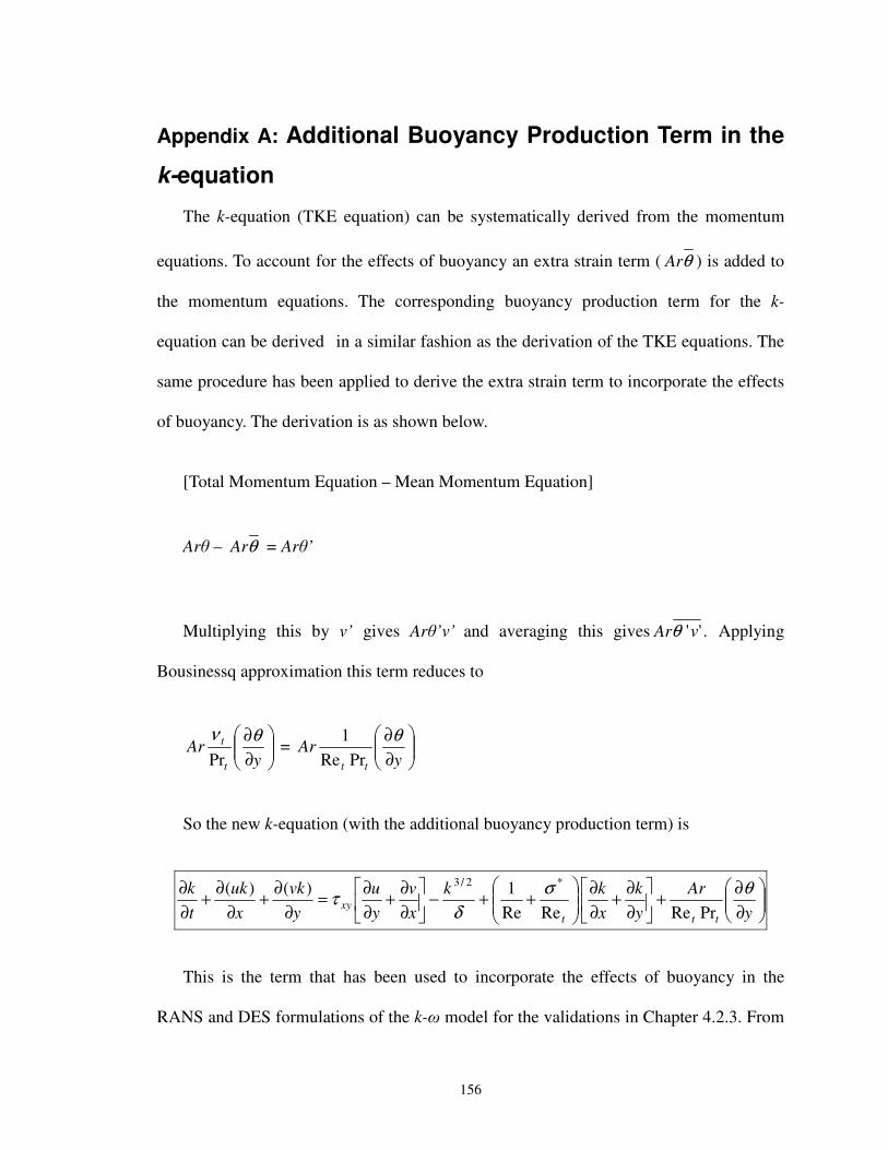
156

Appendix A: Additional Buoyancy Production Term in the

k-equation

The k-equation (TKE equation) can be systematically derived from the momentum

equations. To account for the effects of buoyancy an extra strain term ( θAr ) is added to

the momentum equations. The corresponding buoyancy production term for the k-

equation can be derived in a similar fashion as the derivation of the TKE equations. The

same procedure has been applied to derive the extra strain term to incorporate the effects

of buoyancy. The derivation is as shown below.

[Total Momentum Equation – Mean Momentum Equation] Ar – θAr = Ar’

Multiplying this by v’ gives Ar’v’ and averaging this gives '' vArθ . Applying

Bousinessq approximation this term reduces to

∂∂

yAr

t

t θνPr

=

∂∂

yAr

tt

θPrRe

1

So the new k-equation (with the additional buoyancy production term) is

∂∂+

∂∂+

∂∂

++−

∂∂+

∂∂=

∂∂+

∂∂+

∂∂

yAr

yk

xkk

xv

yu

yvk

xuk

tk

tttxy

θσδ

τPrRe

ReRe

1)()( *2/3

This is the term that has been used to incorporate the effects of buoyancy in the

RANS and DES formulations of the k- model for the validations in Chapter 4.2.3. From

157

this study it was observed that the term had considerable influence on the RANS

predictions, while hardly affecting the DES predictions. Since no differences in the DES

prediction capabilities were noted, this modification had not been incorporated in the

later DES studies (Chapter 5.5).

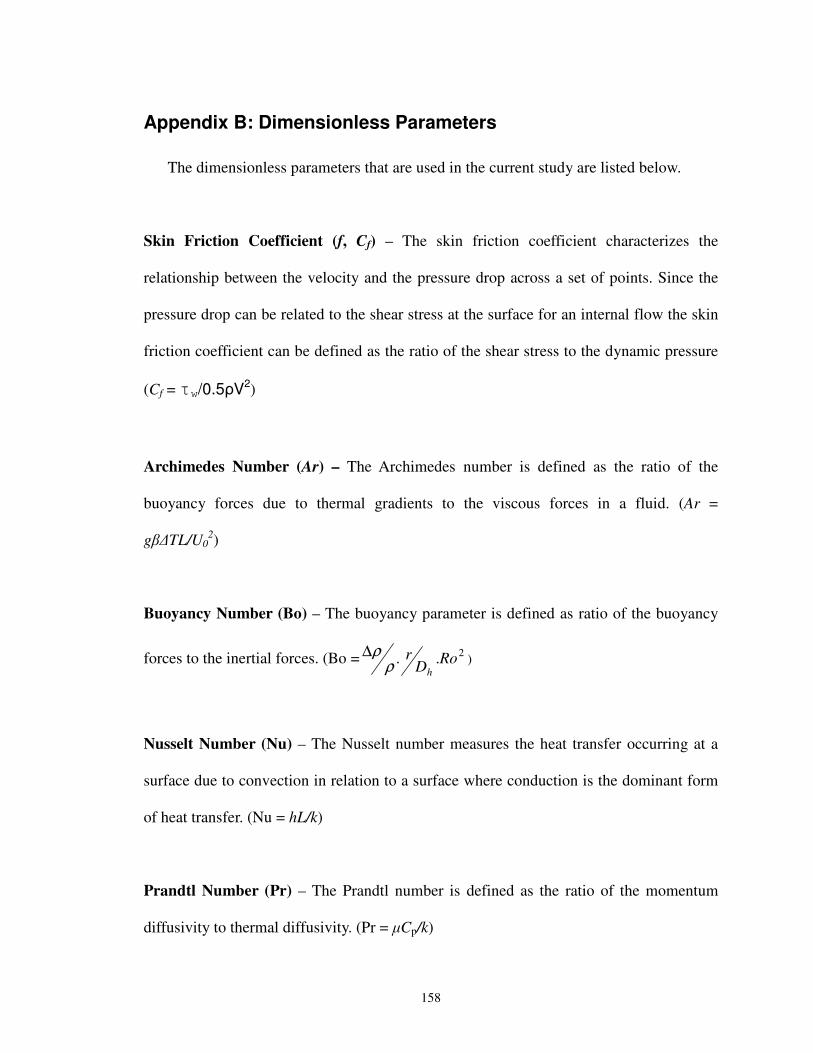
158

Appendix B: Dimensionless Parameters

The dimensionless parameters that are used in the current study are listed below.

Skin Friction Coefficient (f, Cf) – The skin friction coefficient characterizes the

relationship between the velocity and the pressure drop across a set of points. Since the

pressure drop can be related to the shear stress at the surface for an internal flow the skin

friction coefficient can be defined as the ratio of the shear stress to the dynamic pressure

(Cf = w/0.5V2)

Archimedes Number (Ar) – The Archimedes number is defined as the ratio of the

buoyancy forces due to thermal gradients to the viscous forces in a fluid. (Ar =

gTL/U02)

Buoyancy Number (Bo) – The buoyancy parameter is defined as ratio of the buoyancy

forces to the inertial forces. (Bo = 2.. RoDr

hρρ∆ )

Nusselt Number (Nu) – The Nusselt number measures the heat transfer occurring at a

surface due to convection in relation to a surface where conduction is the dominant form

of heat transfer. (Nu = hL/k)

Prandtl Number (Pr) – The Prandtl number is defined as the ratio of the momentum

diffusivity to thermal diffusivity. (Pr = Cp/k)

159

Reynolds Number (Re) – The Reynolds number is defined as the ratio of the inertial

forces to the viscous forces. The Reynolds number determines if the flow is laminar or

turbulent. (Re = VD/)

Rotation Number (Ro) – The rotation number is the ratio of the Coriolis forces in a fluid

to the inertial forces. The rotation number is the reciprocal of the more popular Rossby

number which is used to compare the effects of Coriolis forces. (Ro = L/U)

Richardson Number (Ri) – The Richardson number is the relative importance of the

thermal stratification to the inertial effects of the fluid. The higher the Richardson

number, the more the flow is driven by buoyancy.

160

Appendix C: Abstracts of relevant publications

Viswanathan, A.K., Tafti, D.K., “Detached Eddy Simulation of Turbulent Flow and Heat Transfer in a Ribbed Duct”, ASME Journal of Fluids Engineering, 127(5), pp 888-896, September 2005.

Detached Eddy Simulation (DES) of a hydrodynamic and thermally developed turbulent flow is presented for a stationary duct with square ribs aligned normal to the main flow direction. The rib height to channel hydraulic diameter (e/Dh) is 0.1, the rib pitch to rib height (P/e) is 10 and the calculations have been carried out for a bulk Reynolds number of 20,000. DES calculations are carried out on a 963 grid, a 643 grid and a 483 grid to study the effect of grid resolution. Based on the agreement with earlier LES computations, the 643 grid is observed to be suitable for the DES computation. DES and RANS calculations carried out on the 643 grid are compared to LES calculations on 963/1283 grids and experimental measurements. The flow and heat transfer characteristics for the DES cases compare well with the LES results and the experiments. The average friction and the augmentation ratios are consistent with experimental results, predicting values within 10% of the measured quantities, at a cost lower than the LES calculations. RANS fails to capture some key features of the flow. Viswanathan, A.K., Tafti, D.K., “Detached Eddy Simulation of Turbulent Flow and Heat Transfer in a Two-pass Internal Cooling Duct”, International Journal of Heat and Fluid Flow, 27(1), pp 1-20, February 2006.

Numerical predictions of a hydrodynamic and thermally developed turbulent flow are presented for a stationary duct with square ribs aligned normal to the main flow direction. The rib height to channel hydraulic diameter (e/Dh) is 0.1, the rib pitch to rib height (P/e) is 10 and the calculations have been carried out for a bulk Reynolds number of 20,000. The capability of the Detached Eddy Simulation (DES) version of the 1988 k- model has been validated in predicting the turbulent flow field and the heat transfer in a complete two pass channel. Results of mean flow quantities, secondary flows, friction and heat transfer are compared to experiments and Large-Eddy Simulations (LES). It is concluded that in spite of shortcomings in predicting transition correctly at the entrance to the duct, DES surpasses the base capability of the underlying RANS model and predicts flow and heat transfer with good accuracy in a flow which is dominated by separation and reattachment of shear layers, unsteady vortex induced secondary motions, and strong streamline curvature. In all aspects it reproduces the correct physics and shows good quantitative comparisons with LES and experiments while reducing the computational complexity by nearly an order of magnitude.

161

Viswanathan, A.K., Tafti, D.K., “Detached Eddy Simulation of Flow and Heat Transfer in Fully Developed Rotating Internal Cooling Channel with Normal Ribs”, International Journal of Heat and Fluid Flow, 27(3), pp 351-370, June 2006.

Numerical predictions of a hydrodynamic and thermally developed turbulent flow are

presented for a rotating duct with square ribs aligned normal to the main flow direction. Three rotation numbers Ro=0.18, 0.35 and 0.67 are investigated. The rib height to channel hydraulic diameter (e/Dh) is 0.1, the rib pitch to rib height (P/e) is 10 and the calculations have been carried out for a bulk Reynolds number of 20,000. The capability of the Detached Eddy Simulation (DES) in predicting the turbulent flow field and the heat transfer under the effects of rotation has been evaluated against Unsteady Reynolds-Averaged Navier Stokes (URANS), Large-Eddy Simulations (LES), and experimental data. It is shown that DES by capturing a large portion of the turbulent energy in the resolved scales is much more capable than URANS in transcending the underlying shortcomings of the RANS model. DES shows much better fidelity in calculating critical components of the turbulent flow field and heat transfer than URANS does.

Viswanathan, A.K., Tafti, D.K., “A Comparative Study of DES and URANS for Flow Prediction in a Two-pass Internal Cooling Duct”, In press ASME Journal of Fluids Engineering

The capabilities of the Detached Eddy Simulation (DES) and the Unsteady Reynolds Averaged Navier-Stokes (URANS) versions of the 1988 k- model in predicting the turbulent flow field in a two-pass internal cooling duct with normal ribs is presented. The flow is dominated by the separation and reattachment of shear layers; unsteady vorticity induced secondary flows and strong streamline curvature. The techniques are evaluated in predicting the developing flow at the entrance to the duct and downstream of the 180o bend, fully-developed regime in the first pass, and in the 180o bend. Results of mean flow quantities, secondary flows and the average friction factor are compared to experiments and Large-Eddy Simulations (LES). DES predicts a slower flow development than LES, while URANS predicts it much earlier than LES computations and experiments. However it is observed that as fully developed conditions are established, the capability of the base model in predicting the flow is enhanced by the DES formulation. DES accurately predicts the flow both in the fully-developed region as well as the 180o bend of the duct. URANS fails to predict the secondary flows in the fully-developed region of the duct and is clearly inferior to DES in the 180o bend.

Documents

Detached eddy simulation of turbulent flow and heat transfer in a two-pass internal cooling duct