Detached-Eddy Simulation With Compressibility Corrections Applied to a Supersonic Axisymmetric Base Flow

ondi-com-ulationer therge-endedhigh-etc.).tions,ratestressn bothed, anded onls andflowsdata,

James R. ForsytheAssociate Professor,

Department of Aeronautics,United States Air Force Academy,

USAF Academy, CO 80840

Klaus A. HoffmannProfessor

Department of Aerospace Engineering,Wichita State University,

Wichita, KS 67260

Russell M. CummingsProfessor,

Department of Aerospace Engineering,California Polytechnic State University,

San Luis Obispo, CA 93407

Kyle D. SquiresProfessor,

Department of Mechanical Engineering,Arizona State University,

Tempe, AZ 85287

Detached-Eddy Simulation WithCompressibility CorrectionsApplied to a SupersonicAxisymmetric Base FlowDetached-eddy simulation is applied to an axisymmetric base flow at supersonic ctions. Detached-eddy simulation is a hybrid approach to modeling turbulence thatbines the best features of the Reynolds-averaged Navier-Stokes and large-eddy simapproaches. In the Reynolds-averaged mode, the model is currently based on eithSpalart-Allmaras turbulence model or Menter’s shear stress transport model; in the laeddy simulation mode, it is based on the Smagorinski subgrid scale model. The intapplication of detached-eddy simulation is the treatment of massively separated,Reynolds number flows over complex configurations (entire aircraft, automobiles,Because of the intented future application of the methods to complex configuraCobalt, an unstructured grid Navier-Stokes solver, is used. The current work incorpocompressible shear layer corrections in both the Spalart-Allmaras and shear stransport-based detached-eddy simulation models. The effect of these corrections odetached-eddy simulation and Reynolds-averaged Navier-Stokes models is examincomparisons are made to the experiments of Herrin and Dutton. Solutions are obtainseveral grids—both structured and unstructured—to test the sensitivity of the modecode to grid refinement and grid type. The results show that predictions of baseusing detached-eddy simulation compare very well with available experimentalincluding turbulence quantities in the wake of the axisymmetric body.@DOI: 10.1115/1.1517572#

po

t

ea

e

w

ui

gridallyoreningtly

ow-s in

andto

tur-idealesNS

und-

l re-nrs.iontoer-

y to

adandw

solu-ere

LES

ined

nF

1 IntroductionAs airplanes, missiles, and launch vehicles require greater

formance in ever-expanding flight regimes, the methods andcedures used for their design must be re-evaluated. The theand capabilities that were state of the art only a handful of yeago may not adequately address the design requirements ofrent and future flight vehicles. All aerodynamic predictive meods have as their primary goal the prediction of lift and draSpecifically, a major constraint on the performance of flight vhicles is the total configuration drag. A supersonic body expences major drag contributions from skin friction drag, wave drand pressure drag~especially in the form of base drag!. Obtainingvalid predictions for these drag components, and thus having vtools for design purposes, is difficult at best. Specifically, the pdiction of base drag in an accurate manner has long eludedpracticing engineer. Depending on the vehicle’s base geomand flight conditions, the prediction of base drag can range frmildly irritating to incredibly difficult, yet the importance of basdrag mandates that the engineer be able to make a crediblediction. Experimental and semi-empirical approaches to preding base flow have been attempted for the past 50 years,varying degrees of success. In the past 20 years, various numeapproaches have been used to solve the base flow problem, bnecessity for predicting turbulence in the base region has limthe quality of the predictions,@1,2#.

There are various techniques for the numerical predictionturbulent flows. These range from Reynolds-averaged NavStokes~RANS!, to large-eddy simulation~LES!, to direct numeri-cal simulation~DNS!. DNS attempts to resolve all scales of tu

Contributed by the Fluids Engineering Division for publication in the JOURNALOF FLUIDS ENGINEERING. Manuscript received by the Fluids Engineering DivisioMarch 20, 2002; revised manuscript received July 2, 2002. Associate Editor:Grinstein.

Copyright © 2Journal of Fluids Engineering

per-ro-ries

arscur-h-g.e-ri-g,

alidre-the

etryom

pre-ict-ith

ricalt theted

ofier-

r-

bulence, from the largest to the smallest. Because of this, theresolution requirements are very high, and increase drasticwith Reynolds number. LES attempts to model the smaller, mhomogeneous scales, while resolving the larger, energy contaiscales, which makes the grid requirements for LES significanless than for DNS. To accurately resolve the boundary layer, hever, LES must accurately resolve the energy-containing eddiethe boundary layer, which requires very small streamwisespanwise grid spacing. Finally, the RANS approach attemptssolve the time-averaged flow, which means that all scales ofbulence must be modeled. RANS models often fail to provaccurate results for these flows since the large turbulence scfor separated flows are very dependent on the geometry. RAmodels, however, can provide accurate results for attached boary layer flows and thin shear layers. Spalart@3# provides adiscussion and comparison of these various techniques.

These various techniques have very different computationaquirements. Spalart et al.@4# estimated that the LES computatioover an entire aircraft would not be possible for over 45 yeaTheir estimate led to the formulation of detached-eddy simulat~DES!, which combines the advantages of LES and RANS inone model. RANS is used in the boundary layer, where it pforms well ~and with much lower grid requirements than LES!,and LES is then used in the separated regions where its abilitpredict turbulence length scales is important. Shur et al.@5# cali-brated the model for isotropic turbulence, and applied it toNACA 0012 airfoil section; the model agreed well with lift andrag predictions to 90 deg angle of attack. ConsantinescuSquires@6# applied detached-eddy simulation to the turbulent floover a sphere at several Reynolds numbers. Issues of grid retion, numerical accuracy, and values of the model constant wexamined, and the model was compared to predictions usingand RANS models. Travin et al.@7# applied DES to a circularcylinder at sub and supercritical Reynolds numbers, and obta

,. F.

002 by ASME DECEMBER 2002, Vol. 124 Õ 911

fa

zit

a

t

ss

a

if

a

e

ui

and

ious

d/or

theactw

ons

dient

t;eticthe

,

t is

ffi-ses,th-lyand

n

thesri-isinend

ths to

pro-llysu-

o-us-to

i.e.,andinry-

vier-onsodlu-

olu-ultsbe

uresment

a grid-converged solution that agreed well with experiments. Slets @8# presented numerous cases using DES: a cylinder, airbackstep, triangle in a channel, raised runway section, and a ling gear. Although some cases showed very little improvemover RANS, none performed worse than RANS, and many pformed far better. Forsythe et al.@1# performed DES on the supersonic axisymmetric base flow of Herrin and Dutton@9# using anunstructured solver; good solutions were obtained only by reding the DES constant. This article is an attempt to improve upthese preliminary results by using a larger selection of gridsfurther examine the sensitivity of the model to grid refinemeMenter’s shear stress transport-based DES is used for thetime on this flow, and both RANS and DES models are run wand without compressibility corrections.

2 Base Flow DescriptionBase flows are an important form of separation found in sup

sonic flowfields. This kind of flow is commonly found behinsuch objects as missiles, rockets, and projectiles. The low presfound behind the base causes base drag which can be a siportion of the total drag. To make computational fluid dynamuseful as a design tool, it is important to be able to predictbase pressure accurately.

An axisymmetric base flow depicted with pressure contoursstreamlines is shown in Fig. 1. The large turning angle behindbase causes separation and the formation of a region of revflow ~known as the recirculation region or the separation bubb!.The size of the recirculation region determines the turning anof the flow coming off the back of the base, and thereforestrength of the expansion waves. A smaller recirculation regcauses the flow to turn sharply, leading to a stronger expanwave, and lower pressures behind the base. Therefore, smallrated regions cause larger base drag than large regions.

Directly behind the base, in the recirculation region, the reveflow can be seen. The point along the axis of symmetry wherestreamwise velocity is zero is considered to be the shear lreattachment point. As the shear layer reattaches, the flowforced to turn along the axis of symmetry, causing the formatof a reattachment shock. Figure 1 shows the time average oflowfield; for high Reynolds numbers, the incoming boundalayer and the flow behind the base will be turbulent, leadinghighly unsteady flow behind the base. Bourdon et al.@10# presentplanar visualizations of the large-scale turbulent structures insymmetric supersonic base flows, which provides evidence forunsteadiness and complexity of the flowfield.

Murthy and Osborn@11# provide an excellent overview of thbase flow problem, including a collection of semi-empirical aproaches to model base pressure and base drag, while Det al. @12# provide a good overview on the progress in comput

Fig. 1 Axisymmetric base flow—expansion and shock waves.SST RANS simulation, contours of pressure and streamlines.

912 Õ Vol. 124, DECEMBER 2002

tre-oil,nd-

enter--

uc-onto

nt.firstith

er-dsureable

cshe

ndtheerselegleheionionepa-

rsetheyer

isonthe

ryto

xi-the

p-tton

ng

high-speed separated base flows. Some of the difficultiescomplicating factors in modeling the base flow problem are

1. the upstream effects of the presence of a corner in varMach number flows at different Reynolds numbers;

2. the effects of separation, compression, expansion, anshock formation in the vicinity of the corner;

3. the influence of the expansion wave at the base corner oninitial turbulence structure of the shear layer, and the impof that shear layer on the formation of the recirculating floregion;

4. the shear layer exists under highly compressible conditi~i.e., at high convective Mach numbers!, which alters theturbulence structure,@13–16#;

5. the shear layer encounters a strong adverse pressure graat reattachment;

6. the strong streamline curvature at the reattachment poin7. the enclosed recirculating region imposes a highly energ

and nonuniform upstream velocity at the inner edge ofshear layer;

8. the structure and shape of the recirculating zone; and9. and the effects of the configuration~e.g., diameter, boattail

fins, etc.!.

Taken in total, these flow features yield a complex flowfield thaconsiderably difficult to model analytically or numerically.

3 A Brief Overview Of Experimental and Computa-tional Studies

The complexities of the flow in the base region, and the diculties associated with accurately predicting the flow procesled researchers to utilize various semi-empirical prediction meods which were valuable but limited in their application. Earattempts to predict base flows are summarized by MurthyOsborn@11#, as well as Delery and Lacau@17#. These methodsinclude data correlations~such as those performed by von Karmaand Moore, Hoerner, and Kurzweg! as well as theortically basedmodels~such as the Chapman-Korst component model, andviscid-inviscid integral interaction technique of Crocco and Lee!.These models were limited in applicability by the lack of expemental results for flowfield quantities in supersonic flow. Thispartially due to the difficulty in measuring turbulence quantitiescompressible flow, as well as the difficulty in interpreting thmeaning of what is being measured. According to Murthy aOsborn@11#, future experiments, ‘‘will have to be carried out boto assess the gross effects of various parameters as well aobtain detailed velocity, pressure, enthalpy, and concentrationfiles in the base region.’’ This recommendation was originamade in 1974, and has only been marginally fulfilled in the ening quarter century.

In spite of the importance of the semi-empirical methods, ‘‘slution of the full, Reynolds-averaged Navier-Stokes equationsing currently available numerical methods offers the abilitymore realistically predict the details of the base flow structure,to remove many of the assumptions inherent in the componentintegral techniques.’’@12# Over the past 30 years, advancescomputational capabilities~namely increased computer memosize and processing speed!, as well as improved numerical methods, have enabled attempts at solving various levels of the NaStokes equations for the flow around a base. Early predictiwere limited in size and scope by the solution algorithm methand by capabilities of the computer, but eventually practical sotions were obtained.

Eventually, computations were made using RANS-based stions and algebraic turbulence models, but inadequate resquickly showed that higher-level models for turbulence wouldrequired for base flows@18#. Putnam and Bissinger@19# summa-rize these early attempts and concluded that the current~mid1984! methods were unable to accurately predict the pressafter separation. They also recommended that, ‘‘the assess

Transactions of the ASME

f

ug

i

u

hti

n-

fl

l

n

l

rr

li

ne

e

t

sed

Inood,er-ch-han

theES

u-Theto

ara-rlyuiteedwas

toive.Sorsbrid

ally

-ionityno-.ues

edood.

f its

histiontis-

gra-b-

n.r

od-

f

lly

ach,r ofngandts isratethe

an, ao

criteria of numerical predictions should be based on the surpressure distributions and flowfield characteristics and not simon the overall afterbody drag.’’ Petrie and Walker@20# tested thepredictive capabilities of RANS calculations by soliciting soltions from a number of groups for a power-on base flow confiration, for which they had experimental data~the experimentaldata was not released to the groups performing the calculatio!.Many fundamental parameters such as the base pressure mtude and radial variation, as well as the recirculation region swere not accurately predicted, with large variations amongdifferent groups.

More recently, several groups have obtained results with mbetter agreement, including Benay et al.@21#, Caruso and Childes@22#, Childs and Caruso@23,24#, Peace@25#, Tucker and Shyy@26#, Suzen et al.@27#, Sahu@28#, Chuang and Chieng@29#, andForsythe et al.@30#. Factors that affected the accuracy of tRANS simulation of these flows included the solution-adapgrid alignment in the high gradient shear layer regions andproved turbulence modeling~especially modeling the effects ocompressibility and streamline curvature!. Childs and Caruso@23#suggested that, ‘‘comparison of simply the base pressure betwcomputation and experiment, without any complementary flofield data, can lead to false conclusions regarding the accuracthe numerical solutions, due to cancellation of errors causedinaccurate turbulence modeling and insufficient grid resolutioDutton et al.@12# also state that, ‘‘the difficult problem of turbulence modeling is the most critical outstanding issue in the acrate RANS predictions of these complex flows.’’

Since Herrin and Dutton@9# published their detailed experimental results on aM`52.46 axisymmetric supersonic base flow, seeral researchers have performed RANS computations on thisattempting to find an accurate RANS turbulence model. Sahu@28#used two algebraic turbulence models~Baldwin-Lomax andChow! and Chien’s low Reynolds numberk2e model. Chuangand Chieng@29# published results for three higher-order modelstwo-layer algebraic stress model, Chien’s two-equationk2emodel, and Shima’s Reynolds stress model. Tucker and Shyy@26#used several variations of two-equationk2e models, includingthe original Jones-Launder formulation, and extensions to alimproved response to the mean strain rate and compressibeffects. Both Sahu’sk2e computation and Chuang and ChiengReynolds stress prediction of the base pressure were in reasoagreement with the experimental results. However, all of the mels poorly predicted the mean velocity and turbulence fields. Aeven though all three studies employed a ‘‘standard’’k2e model,they obtained substantially different predictions of the base psure distribution. This points to possible dependence on numeimplementation, grid resolution, turbulence model implemention, and/or boundary conditions. Suzen et al.@27# tested severapopular RANS models on a two-dimensional base, and obtagood agreement for base pressure by adding compressibilityrections to Menter’s model. Forsythe et al.@30# applied severalRANS models to the two-dimensional and axisymmetric baAlthough the two-dimensional base pressure was well predicby two-equation models with compressibility corrections,model predicted the constant pressure profile for the axisymmbase.

Based on the unsatisfactory results of RANS calculationsdate, other approaches such as large-eddy simulation or dnumerical simulation should be considered. Dutton et al.@12#state that, ‘‘In order to avoid the difficulties inherent in turbulenmodeling for the Reynolds-averaged Navier-Stokes~RANS! ap-proach, the large-eddy simulation~LES! or direct numerical simu-lations~DNS! techniques will eventually be applied to high-speflows.’’ Harris and Fasel@31# performed DNS on aM`52.46two-dimensional base flow with the goal of addressing, ‘‘the nture of the instabilities in such wake flows and to examinestructures that arise from these instabilities.’’ Fureby et al.@32#performed large-eddy simulation on the axisymmetricM`52.46

Journal of Fluids Engineering

aceply

-u-

nsagni-ze,the

ch

eedm-f

eenw-y ofby.’’

cu-

-v-ow,

: a

owility’sable

od-so,

es-icalta-

nedcor-

se.tedotric

toirect

ce

d

a-he

base flow of Mathur and Dutton@33# and Herrin and Dutton@9#,including the effects of base bleed. Subgrid scale models uwere the Monotone Integrated LES~MILES! model, the one-equation eddy-viscosity model, and the Smagorinski model.general, agreement with the experimental data were quite ghowever, the size of the recirculation region was slightly undpredicted. A potential source of error cited was that the approaing boundary layer thickness in the computations was smaller treported in the experimental data. This is presumably becausegrid resolution in the boundary layer was inadequate for an Lcomputation, although the grid was not shown.

Forsythe et al.@1# applied detached-eddy simulation on the spersonic axisymmetric base flow using an unstructured solver.boundary layer was treated entirely by RANS, which was ableadequately predict the boundary layer thickness prior to seption. Two grids were used, with the coarse grid being cleainadequate. The fine grid gave a DES solution that agreed qwell with experiments if the DES model constant was reducenough. Although the good agreement with the experimentsencouraging, the lack of a grid-refined solution, and the needadjust the DES constant kept the results from being conclusAdditionally, the poor performance of the Spalart-Allmaras RANmodel on this flow created skepticism on the part of the auththat the Spalart-Allmaras model was a good base for a hymodel for this flow. Menter’s model and Wilcox’sk2v modelperformed far better than the Spalart-Allmaras model, especiwhen compressibility corrections were included.

Baurle et al.@34# later explored hybrid RANS/LES for the supersonic axisymmetric base flow. A separate RANS simulatwas run upstream of the base to obtain a fully turbulent velocprofile of the correct thickness just prior to the base, then a motone integrated LES~MILES! was performed in the base regionThis approach allowed the authors to examine numerical iss~apart from modeling issues! since a pure LES approach was usbehind the base. The agreement with experiments was quite g

4 Governing Equations And Flow SolverThe unstructured flow solver Cobalt was chosen because o

speed and accuracy~Cobalt is a commercial version of Cobalt60).The relevant improvements in the commercial version for tstudy were the inclusion of SST-based DES, faster per-iteratimes, the ability to calculate time-averages and turbulent statics, an improved spatial operator, and improved temporal intetion. Strang et al.@35# validated the code on a number of prolems, including the Spalart-Allmaras model~which forms the coreof the DES model!. Tomaro et al.@36# converted Cobalt60 fromexplicit to implicit, enabling CFL numbers as high as one millioGrismer et al.@37# then parallelized the code, yielding a lineaspeedup on as many as 1024 processors. Forsythe et al.@30# pro-vided a comprehensive testing and validation of the RANS mels: Spalart-Allmaras, Wilcox’sk2v, and Menter’s models. TheParallel METIS ~ParMetis! domain decomposition library oKarypis and Kumar@38# and Karypis et al.@39# is also incorpo-rated into Cobalt. ParMetis divides the grid into nearly equasized zones that are then distributed among the processors.

The numerical method is a cell-centered finite volume approapplicable to arbitrary cell topologies~e.g, hexahedrals, prismstetrahdra!. The spatial operator uses the exact Riemann solveGottlieb and Groth@40#, least squares gradient calculations usiQR factorization to provide second-order accuracy in space,TVD flux limiters to limit extremes at cell faces. A point implicimethod using analytic first-order inviscid and viscous Jacobianused for advancement of the discretized system. For time-accucomputations, a Newton subiteration scheme is employed, andmethod is second-order accurate in time.

The compressible Navier-Stokes equations were solved ininertial reference frame. To model the effects of turbulenceturbulent viscosity (m t) is provided by the turbulence model. Tobtainkt ~the turbulent thermal conductivity!, a turbulent Prandtl

DECEMBER 2002, Vol. 124 Õ 913

b

stt

ecd

no

e

c

l

l

by

l.imu-ier-ows

-Thetion

ion

aleid

ski

-torye

(

ll

STby

th

nedlude

ofhd

in

tet-in

smsellsom-ly,

gth

fgesten-gths-of-griden-

number is assumed with the following relation: Prt5cpm t /kt50.9. In the governing equations,m is replaced by (m1m t) andk~the thermal conductivity! is replaced by (k1kt). The laminarviscosity,m, is defined using Sutherland’s law.

5 Spalart-Allmaras „S-A… ModelThe Spalart-Allmaras~SA! one-equation model,@41# solves a

single partial differential equation for a variablen which is relatedto the turbulent viscosity. The differential equation is derived‘‘using empiricism and arguments of dimensional analysis, Gilean invariance and selected dependence on the molecular viity.’’ The model includes a wall destruction term that reducesturbulent viscosity in the log layer and laminar sublayer, andterms that provide a smooth transition from laminar to turbuleFor the current research, the trip term was turned off. Spalart@42#suggested the use of the compressibility correction of Secun@43#. In order to effect the correction, the following destructioterm is added to right-hand side of the Spalart-Allmaras moequation:

2C5n2Ui , jUi , j /a2 (1)

wherea is the speed of sound andC553.5, which is empiricallydetermined. The term accounts for the reduced spreading rata compressible shear layer by reducing the turbulent eddy visity. Cases run with the compressibility correction active arenoted by ‘‘CC.’’

6 Menter’s Shear Stress Transport ModelWilcox’s k2v model is well behaved in the near-wall regio

where low Reynolds number corrections are not required. Hever, the model is generally sensitive to the freestream valuev. This sensitivity seems to be a factor mainly for free shflows, and does not seem to adversely affect boundary layer floOn the other hand, thek2e equations are relatively insensitive tfreestream values, but behave poorly in the near wall region,@44#.Menter @45,46# proposed a combinedk2e/k2v model ~knownas Menter’s SST model! which uses the best features of eamodel. The model uses a parameterF1 to switch fromk2v tok2e in the wake region to prevent the model from being sensitto freestream conditions.

Menter did not include compressibility corrections in hmodel. Suzen and Hoffmann@47#, however, added compressibdissipation and pressure dilatation terms to thek2e portion ofMenter’s model. When Menter’s blending process is applied,following equations result:

D

Dt~rk!5t i j

]ui

]xj1~12F1!p9d92b* rvk~11a1Mt

2~12F1!!

1]

]xjF ~m1skm t!

]k

]xjG (2)

D

Dt~rv!5

gr

m tt i j

]ui

]xj1~12F1!b* a1Mt

2rv2

1]

]xjF ~m1svm t!

]v

]xjG2brv212r~12F1!sv2

31

v

]k

]xj

]v

]xj2~12F1!

p9d9

n t(3)

where the pressure dilatation term is

p9d952a2t i j

]ui

]xjMt

21a3reMt2 (4)

and the closure coefficients for the compressible correctionsa151.0, a250.4, anda350.2. By adding these corrections onto the k2e portion of the model, the near wall solution (k2v


y,al-cos-heripnt.

dovndel

s inos-e-

,w-

s ofarws.

o

h

ive

ise

the

are:y

portion! is unaffected, as observed by Forsythe et al.@48#. Casesrun with the compressibility correction active are denoted‘‘CC.’’

7 Detached-Eddy Simulation„DES…Detached-eddy simulation~DES! was proposed by Spalart et a

@4# as a method to combine the best features of large-eddy slation with the best features of the Reynolds-averaged NavStokes approach. RANS tends to be able to predict attached flvery well with a low computation cost. Traditional LES~i.e., LESwithout using a wall model!, on the other hand, has a high computation cost, but can predict separated flows more accurately.model was originally based on the Spalart-Allmaras one-equaRANS turbulence model discussed above and in@41#. The walldestruction term is proportional to (n/d)2, whered is the distanceto the closest wall. When this term is balanced with the productterm, the eddy viscosity becomesn}Sd2, whereS is the localstrain rate. The Smagorinski LES model varies its subgrid-sc~SGS! turbulent viscosity with the local strain rate and the grspacing,D ~i.e., nSGS}SD2). If, therefore,d is replaced byD inthe wall destruction term, the S-A model will act as a SmagorinLES model.

To exhibit both RANS and LES behavior,d in the SA model isreplaced by

d5min~d,CDESD! (5)

whereCDES is the DES model constant. Whend!D, the modelacts as a RANS model. Whend@D, the model acts as a Smagorinski LES model. Therefore, the model can be ‘‘switched’’LES mode by locally refining the grid. In an attached boundalayer, a RANS simulation will have highly stretched grids in thstreamwise direction. To retain RANS behavior in this case,D istaken as the largest spacing in any directionD5max(Dx,Dy,Dz)). The model was calibrated by Shur et al.@5#using isotropic turbulence to giveCDES of 0.65. AlthoughCDESwas reduced previously,@1#, the current study uses 0.65 for acases.

Strelets@8# introduced a DES model based on Menter’s Smodel. In the SST model, the turbulent length scale is givenl k2v5k1/2/(b* v). The DES modification replaces the lengscale by l 5min(lk2v ,CDESD) in the dissipative term of thek-transport equation~i.e., the dissipation term isDDES

k 5rk3/2/ l ).Since the compressibility corrections outlined above are desigto decrease the turbulence length scale, it was decided to incthem in the equation forl ~i.e., l k2v5k1/2/(b* (11a1Mt

2(12F1))v)). Since Menter’s SST model is based on a blendingk2e andk2v, Strelets@8# calibrated the model by running botthek2e andk2v DES models on isotropic turbulence. This leato CDES

k2e50.61 andCDESk2v50.78. The traditional blending function

was used to blend between the two constants~i.e., CDES5(12F1)CDES

k2e1F1CDESk2v). The recommended constants were used

the current study.Since Cobalt accepts arbitrary cell types, a combination of

rahedra and prisms were used in the current study. This iscontrast to structured grids which use hexahedral cells. Priwere used in the boundary layer to reduce the number of cneeded and to increase the accuracy of the boundary layer cputation by increasing the orthogonality of the cells. PreviousForsythe et al.@1# used the longest edge in each cell asD. How-ever it was pointed out that a tetrahedron with an edge lenequal to a hexahedron will have roughly 1/6th the volume~imag-ine a cube cut into 6 tetrahedra!. A more consistent method odefining the length scale is used in the current study—the lardistance between the cell center and all the neighboring cell cters. Since Cobalt is cell-centered, this definition provides a lenscale based on the distance between neighboring degreefreedom. In the current study, the streamwise and spanwisespacing was slightly larger than the boundary layer thickness,


t

-d

crt

e

u

y

h

a

fi

1h

r

w5r

into

suring that the model was operating in a RANS mode inboundary layer~sinced,D in the boundary layer!.

8 ResultsThe current article is an attempt to resolve many of the iss

revealed in the previous study,@1#, in order to build confidence inDES for compressible flows. Four grids~both structured and unstructured! are used to examine the sensitivity of the DES moto grid refinement and grid type. DES based on Menter’s shstress transport model is applied to determine the sensitivityDES on the RANS model for this flow. Compressibility corretions are applied to both Spalart-Allmaras and shear sttransport-based DES. Comparisons are made to RANS soluand experiments.

8.1 Test Conditions. The experimental conditions for thaxisymmetric base of Herrin and Dutton@9# were matched in thecurrent computations. Freestream conditions ofM`52.46 and aunit Reynolds number of Re5453106 per meter were imposed athe inflow boundary. With a base radius of 31.75 mm, the resing Reynolds number based on the diameter was Re52.8583106. The test conditions are summarized in Table 1.

8.2 Grids and Boundary Conditions. Two unstructuredgrids and two structured grids were used in the current studexamine the effects of grid resolution and grid type. All grids usa cylinder of length 8R, whereR is the base radius. This lengtwas determined by running Wilcox’s boundary layer codEDDYBL, @49#, with the Spalart-Allmaras model to see whlength was needed to match the experimental momentum thness.

The two structured grids were provided by Baurle et al.@34#,with the fine grid shown in Fig. 2~a!. The grids contained only ashort portion upstream of the base, so an additional set of powas added to extend the cylinder upstream to 8R. Two grids wereused, with the fine grid having twice as many points in eacoordinate direction. The grid densities of the coarse andgrids were 330,000 and 2.603106, respectively. The average firsy1 for the coarse grid on a Spalart-Allmaras calculation waswhile the fine grid was half that value. This is well above trecommended value ofy151 @42#. Since Baurle et al.@34# wereusing wall functions, this spacing was adequate. In the curstudy, however, the boundary layer was treated without the uswall functions, so the resolution was inadequate. The outflowplaced 10R downstream, while the farfield boundary was at 4.1Rfrom the axis of symmetry. The structured coarse and fine gare denoted by SGC and SGF, respectively.

The two unstructured grids had the same basic dimensioneach other. The outflow boundary was placed 12R downstream,and the experimental wind tunnel walls were modeled as aboundary at 10R from the axis of symmetry. The first unstructuregrid, pictured in Fig. 2~b! was created using VGRIDns@50#, and

Table 1 Test conditions for the axisymmetric base flow, †9‡

M` 2.46

r` 0.7549kg

m3

p` 3.14153104N

m2

T` 145 K

Re453106

mR 31.75 mm

U`5U0593.8

m

sec


he

ues

elearof-

essions

tlt-

toed

e,t

ick-

ints

chnet4,e

ente ofas

ids

s as

slipd

was used for previous computations,@1#. Although VGRIDns is apure tetrahedral grid generator, a Cobalt utilityblacksmithwasused to recombine the tetrahedra in the boundary layer

Fig. 2 Closeup views of grids used. „a… Fine structural grid„SGF…—2.60Ã106 cells; „b… VGRIDns grid „VG…—2.86Ã106

cells; „c… Gridgen grid „GG…—2.75Ã106 cells.


td

oi

e

aao

nied.ateudyl

amnethe

rix

toted

deANS

cal-

therethat

, byasand

s-256

ime,tera-

prisms. The average firsty1 spacing was 0.7 for the SpalarAllmaras model, with cells concentrated in the shear layer anthe separated region. The grid consisted of 2.863106 cells, and isdenoted by ‘‘VG.’’ ~See Fig. 3.!

The second unstructured grid was created with Gridgen@51#,and is shown in Fig. 2~c!. This grid was created using the concepin the ‘‘Young-Person’s Guide to Detached-Eddy SimulatiGrids,’’ @52#. Gridgen’s multiblock unstructured gridding capabity was used to pack points in the separated region~or focusregion @52#! to give better LES resolution. Approximately half othe 2.753106 cells were in a region that extended 4R down-stream, and 1.3R from the axis of symmetry. The boundary layconsisted of prisms, with an average firsty1 spacing of less than0.2 for the Spalart-Allmaras model. This grid is denoted‘‘GG.’’

All farfield, inflow, and outflow boundaries used the modifieReimmann invarient boundary condition in Cobalt. It shouldnoted that no synthetic turbulence was added to the farfiboundaries. This was considered appropriate even for DES sthe boundary layer was treated in RANS mode. It was expecthat the instabilities at the separation point would then provideunsteady content for the simulation. Solid walls on the cylindwere set to be adiabatic no slip, while the outer wind tunnel wwere set to a slip boundary condition. For the no-slip boundconditions, the normal gradient of pressure was assumed tzero. No wall functions were used for the turbulence modelsther for DES or RANS.

Fig. 3 Boundary layer profile 1 mm prior to the base—RANSmodels


-in

tsn

l-

f

r

by

dbeeldincetedtheerllsrybe

ei-

8.3 Calculation Details. A timestep study was performedpreviously and reported in@1#. Pressure was monitored at telocations along the axis of symmetry, and the timestep was varAlso, two full DES calculations were done with a timestep thvaried by a factor of two, with little effect on the mean flow. Thcurrent calculations reduced the timestep from the previous stvalue of 5.031026 to 3.231026. This gives a nondimensionatimestep~by base diameter and freestream velocity! of 0.025. Inthe base region, the velocities are far lower than the freestrevelocity, leading to local CFL numbers that are less than ooutside the boundary layer. The other parameters used fortemporal integration were two Newton subiterations, 32 matsweeps, and a temporal damping of 0.025~inviscid! and 0.01~viscous!. The calculations were run for 4000 iterations priorbeginning to take time averages, and statistics were calculainternally by Cobalt for a minimum of 10,000 iterations. The cowas run second-order accurate in both time and space, and Rcalculation were done with a CFL of 13106 to rapidly obtain asteady-state solution. Previous runs suggested that the RANSculations would not give an unsteady solution.

As in the previous study, asymmetries were observed inmean flow. In the previous study, only 4000 total iterations weused to calculate time averages. The current study showedthese asymmetries were greatly reduced, but not eliminatedrunning as many as 40,000 iterations. This many iterations wconsidered impracticable, so averages were taken both in timein the azimuthal direction.

Calculations were performed on an IBM SP3 and a Linux cluter, with between 32 and 256 processors being used. Withprocessors, the most expensive calculations~14,000 iterations,2.853106 cells, DES-SST model! took around 30 wall-clockhours. The steady-state calculations took about a tenth that tsince less than 2000 iterations were necessary with less subi

Fig. 4 Pressure along the base—RANS models

Table 2 Test matrix showing range of time averaged pressure coefficient across the base—take from Figs. 4 and 9. Turbulence models: SA ÄSpalart-Allmaras, SST ÄMenter’s shear stresstransport, DES Ädetached-eddy simulation, CC Äcompressibility correction; Grids: SGCÄstructured grid coarse, SGF Ästructured grid fine, VG ÄVGRIDns grid, GG ÄGridgen grid.

SGC SGF VG GG

SA 20.174/20.192SA-CC 20.082/20.148SST 20.123/20.141SST-CC 20.075/20.128DES-SA 20.117/20.172 20.107/20.118 20.097/20.102 20.098/20.101DES-SA-CC 20.122/20.165 20.097/20.102 20.099/20.102DES-SST 20.088/20.094 20.088/20.090DES-SST-CC 20.093/20.100 20.094/20.097Experimental@9# 20.100/20.105


m

t

ell

eod-

the.

his

lart-a

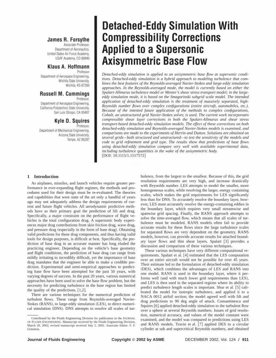
tions. The test matrix for the turbulence models and the differgrids is shown in Table 2. The matrix contains the range of tiaveraged pressure coefficients on the base for each calculatiowell as the experimental values. These values were obtainedfinding the maximum and minimum pressure coefficients froFigs. 4 and 9 in the range measured experimentally. All ofRANS runs were performed on the VGRIDns grid, since RAN

Fig. 5 Centerline velocity—RANS models


ente

n asby

mheS

calculations on that grid were shown previously to match wwith a more fine two dimensional structured grid~see @1# andForsythe et al.@30#!.

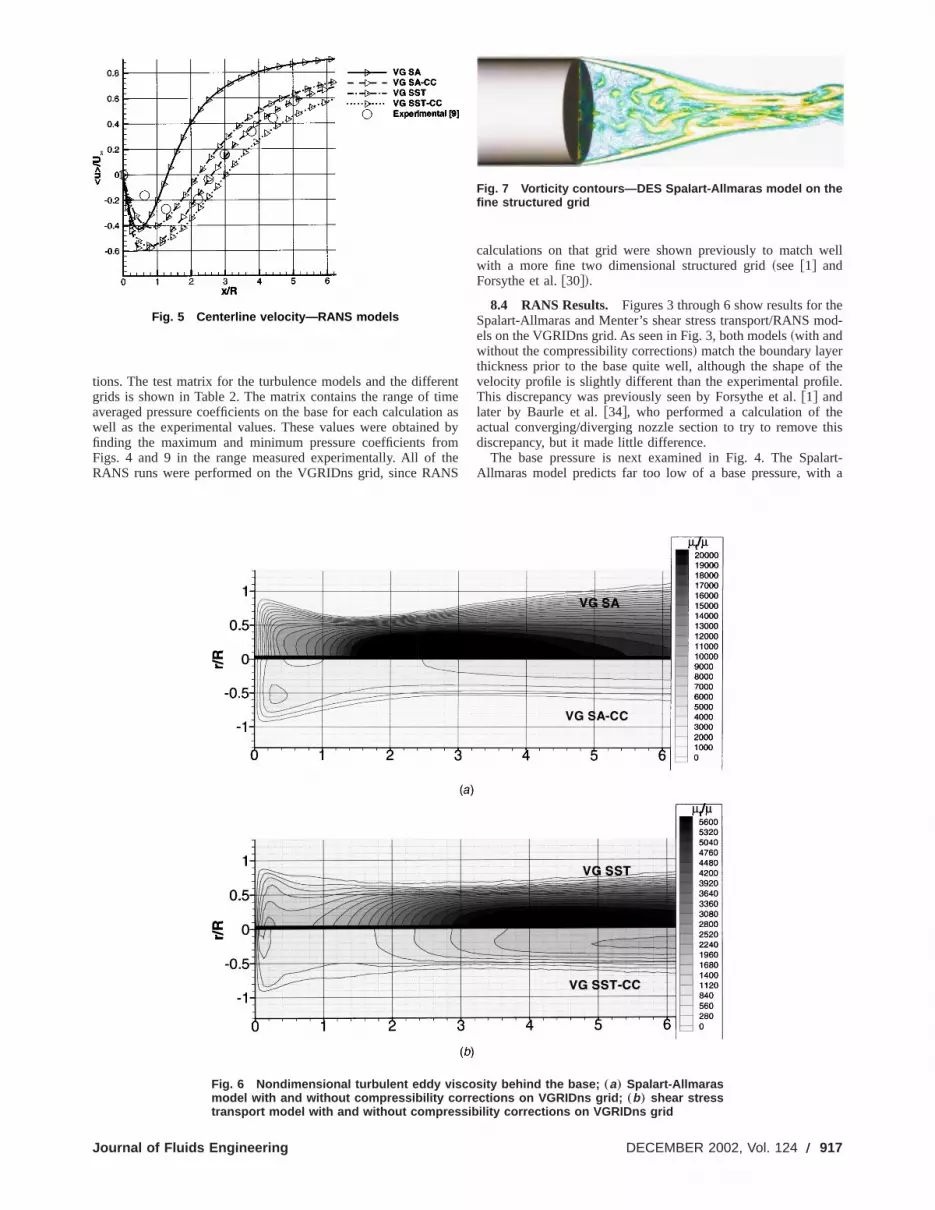
8.4 RANS Results. Figures 3 through 6 show results for thSpalart-Allmaras and Menter’s shear stress transport/RANS mels on the VGRIDns grid. As seen in Fig. 3, both models~with andwithout the compressibility corrections! match the boundary layerthickness prior to the base quite well, although the shape ofvelocity profile is slightly different than the experimental profileThis discrepancy was previously seen by Forsythe et al.@1# andlater by Baurle et al.@34#, who performed a calculation of theactual converging/diverging nozzle section to try to remove tdiscrepancy, but it made little difference.

The base pressure is next examined in Fig. 4. The SpaAllmaras model predicts far too low of a base pressure, with

Fig. 7 Vorticity contours—DES Spalart-Allmaras model on thefine structured grid

Fig. 6 Nondimensional turbulent eddy viscosity behind the base; „a… Spalart-Allmarasmodel with and without compressibility corrections on VGRIDns grid; „b … shear stresstransport model with and without compressibility corrections on VGRIDns grid


tir

.

dnw

f

ofsedheeems of

isolu-us

8.per

maytch

gridtherid

flat-

bleodres-

pre-Theeri-

argainthedelraredonis

isic-

oussultsto

grid.yerticis

, byThe

the

slight radial variation. The compressibility correction has a stroeffect, putting the results much closer to the experiments,introducing a larger radial variation. The SST model without tcompressibility corrections does about as well as SA withcorrection, and with a flatter radial profile. The compressibilcorrection then further improves the pressure level; howeveagain introduces more radial variation.

The centerline velocity behind the base is next plotted in FigThe SA model greatly underpredicts the shear layer reattachmlocation. The peak reverse velocity is overpredicted by the mowith compressibility corrections, which helps explain the icreased variation in pressure along the base. Streamlines floalong the centerline towards the base stagnate on the center obase, leading to the high pressure seen there. The large reduin turbulent eddy viscosity seen in Fig. 6~a! has the effect ofincreasing the recirculation region size, which makes the turnangle at the base more realistic, but allows a larger reverse veity, which leads to a larger variation in pressure. The SST mostarts with much lower turbulent viscosity than SA, as seen in F6~b!, which allows for the larger recirculation region as seenFig. 5. The compressibility correction further reduces the levelseddy viscosity, increasing the size of the recirculation regionther, and increasing the peak reverse velocity.

Fig. 8 Boundary layer profile 1 mm prior to the base—DESmodel

Fig. 9 Pressure along the base—DES model


ngbuthehety, it

5.entels-ing

f thection

ingloc-delig.inof

ur-

8.5 DES Results. Figure 7 shows an instantaneous plotvorticity contours in a cross-plane behind the base for DES baon Spalart-Allmaras on the fine structured grid. Although tshear layer roll up was not captured, the turbulent structures sotherwise well resolved. This figure as well as subsequent plotresolved turbulent kinetic energy provide evidence that DESoperating in LES mode behind the base. Three-dimensional vmetric rendering of isosurfaces of vorticity showed numerosmall scale structures behind the base.

Boundary layer profiles for all DES runs are plotted in Fig.The coarse and fine structured grids fail to predict the proboundary layer thickness due their large average firsty1 values of14 and 7, respectively; coarse streamwise grid spacing alsohave contributed to this underprediction. All other profiles mareasonably well.

The base pressure is plotted in Fig. 9. The coarse structuredis clearly underresolved. The compressibility correction aidsresult somewhat, but not significantly. The fine structured gunderpredicts the base pressure by about 10% but has thepressure profile observed experimentally.~Note that the base pressure for this grid was plotted incorrectly in Forsythe et al.@53#.!The poor boundary layer prediction on this grid is a possisource of error. Both unstructred grid DES-SA results are in goagreement with the experiments, and are insensitive to the pence of the compressibility corrections. The SST results overdict the base pressure by 5%–10%, depending on the grid.compressibility correction moves the pressure towards the expmental values.

The centerline velocity plotted in Fig. 10 exhibits a similbehavior as the grid is varied. The coarse structured grid is aunderresolved, giving a high peak reverse velocity too close tobase. The fact that LES without an explicit subgrid scale mo~predicted by Forsythe et al.@1#! gives a much better result fobase pressure and centerline velocity on the coarse grid compwith DES shows that there is a significant effect of the modelthis grid, in addition to the numerical errors. The nature of DESthat the coarse grid limit yields a RANS model. As the gridrefined, the eddy viscosity will drop lower than a RANS predtion, yet may still be too high to allow an LES prediction.

Mach contours are compared to the experiments for varimodels and grids in Figs. 11. Besides the coarse grid, the reall look quite similar, even when comparing SA-based DESSST-based DES, and the fine structured vs. an unstructuredFigure 11 shows that DES is able to predict a realistic shear lagrowth on the various grids. Plots of resolved turbulent kineenergy~Fig. 12!, however, suggest that the shear-layer rollupnot being resolved. The shear-layer growth is aided, howeverthe presence of turbulent eddy viscosity as seen in Fig. 13.turbulent kinetic energy is underpredicted on all grids~Fig. 12!,especially in the shear layer. Grid refinement should enhance

Fig. 10 Centerline velocity—DES model


Journal of Fluids E

Fig. 11 Mach contours behind the base; „a… DES Spalart-Allmaras on the coarse struc-tured grid versus Experiment †9‡; „b… DES Spalart-Allmaras on the fine structured gridversus Experiment †9‡; „c… DES Spalart-Allmaras on the Gridgen grid versus Experiment†9‡; „d… DES shear stress transport model on Gridgen grid versus Experiment †9‡

ngineering DECEMBER 2002, Vol. 124 Õ 919

920 Õ Vol. 124, D

Fig. 12 Resolved turbulent kinetic energy behind the base; „a… DES Spalart-Allmarasmodel on the coarse structured grid versus Experiment †9‡; „b… DES Spalart-Allmarasmodel on the fine structured grid versus Experiment †9‡; „c… DES Spalart-Allmaras modelon the Gridgen grid versus Experiment †9‡

te

,

edd

ellsfrom

edse

agreement with the experiments, but since some turbulence isbeing modeled~especially in the shear layer!, the mean flow prop-erties are reasonable. The fine structured grid underpredictsshear layer growth rate, which is likely to be the cause forunderprediction of the base pressure. This could be becausstructured grid has finer grid resolution in the shear layer, lowing the eddy viscosity below RANS levels. However, as preously mentioned, the shear layer rollup is not being resolvedthe model is not acting in LES mode.

ECEMBER 2002

still

thehe

theer-vi-

so

It should be noted that the VGRIDns grid was previously usby Forsythe et al.@1#, yet the current results are much improvewith the standard model constant,Cdes50.65. This is partiallyattributed to the redefinition of the length scale on tetrahedral cas discussed previously. Part of the improvement also comesimprovements in the time-accuracy of Cobalt over Cobalt60. Thisevaluation is based on the fact that a calculation was performusing Cobalt60 after the redefinition of the length scale, with ba


Journal of Fluids E

Fig. 13 Nondimensional turbulent eddy-viscosity behind the base; „a… DES Spalart-Allmaras model with and without compressibility corrections on Gridgen grid, „b… DESshear stress transport model with and without compressibility corrections on Gridgengrid

re

E

al

oa

s

hile.un-ol-ob-ESS

id.—ahetoadthewallsureder-

alltions

asESs-

nt onures

ase

pressures and levels of resolved turbulent kinetic energy sowhere between that seen in Forsythe et al.@1# and the currentstudy.

Figure 14 shows turbulent statistics for DES-SA on the Gridggrid. Although underpredicting the statistics in general, the agment is fair. The resolved radial turbulence intensity is furthfrom the experiments.

9 ConclusionsA detailed testing of DES based on both the Spalart-Allma

and the shear stress transport model was conducted on the ssonic axisymmetric base of Herrin and Dutton@9#. The grids wereconstructed so that the boundary layer would be treated fullyRANS mode. Comparisons were made to the Spalart-Allmaand shear stress transport RANS models and experiments. Cpressibility corrections were examined for the RANS and Dmodels.

Both the SA and the SST RANS models seem unable to retically model this flowfield, with Mach contours for both modebeing in significant disagreement with the experimental daCompressibility corrections aid the models in predicting a mrealistic level of pressure on the base, but increase the radial vtion of the pressure due to the increased centerline velocity. Din contrast, predicts a flat pressure profile due to its abilitymodel the unsteady flow that helps equalize the base presDES successfully predicted the boundary layer thickness prio

ngineering

me-

enee-st

rasuper-

inrasom-S

lis-sta.reria-

ES,toure.

r to

the base by operating in RANS mode in the boundary layer, wretaining LES’s ability to predict the flat base pressure profile

Calculations were performed on two structured and twostructured grids to examine the effect of grid resolution and topogy. Good agreement with experimental base pressure wastained on all but the coarse structured grid. The coarse grid Dresults were actually quite similar to the Spalart-Allmaras RANresults with the compressibility correction active on a fine grThis highlights the need for assessing the resolution of the gridfact that is true for RANS, and crucial for DES. The use of tDES modification drew down the eddy viscosity low enoughimprove the poor Spalart-Allmaras RANS results, mimickingcompressibility correction, yet not low enough to allow for gooLES content. The fine structured grid DES underpredictedboundary layer thickness prior to the base due to coarsenormal spacing. This grid also underpredicted the base presby about 10%, although this is not necessarily due to the unprediction of the boundary layer thickness. thickness is quite smcompared to the base diameter. Unstructured grids gave soluthat agreed well with the experimental data.

The sensitivity of DES on the underlying RANS model wexamined by running both Spalart-Allmaras and SST-based Dwith and without compressibility corrections. Spalart-Allmarabased DES predicted the base pressure to within a few percethe unstructured grids. SST-based DES predicted higher pressthan the experiments~the worst disagreement was 10%!. Com-pressibility corrections helped improve the agreement with b


922 Õ Vol. 124,

Fig. 14 Resolved turbulent statistics on the Gridgen grid; „a… resolved streamwise turbu-lent intensity versus Experiment †9‡, „b… resolved radial turbulence intensity versus Experi-ment †9‡, „c… resolved Reynolds stress versus Experiment †9‡

d

d

te

cn

NSds,the

ereata.ust

nd

pressure for the SST-based DES, however, the turbulent eviscosity contours were so similar it is difficult to understand treason for the improvement. Compressibility corrections hanegligible impact on Spalart-Allmaras-based DES. The lacksensitivity of DES to the underlying RANS model is likely duethe fact that the role of the RANS model within DES is confinmainly to the boundary layer and the thin shear layers.

The results of this study show that it is now possible to acrately model axisymmetric base flowfields using appropriate

DECEMBER 2002

dy-he

aofod

u-u-

merical techniques, turbulence models, and grids. While RAturbulence models give relatively poor results for these flowfieland pure LES models are excessively expensive to use ifboundary layer is to be resolved, the hybrid DES models wable to give good comparisons with available experimental dThe DES results also show, however, that careful attention mbe paid to grid size and density, and boundary conditions~espe-cially the inflow boundary layer profile!. While this study wasable to sufficiently match the detailed flowfield data of Herrin a


o—

.

a

w

ad

dr

,

e

L

d

i

d

t

s

a

a

p

o

n

e

c

forper

ase

is--

m-

w

ofper

pe-

uta-

rale,’’

ady

of

lin-

‘AnNS/

th-w

mo.

98,v.

gter

phof

forut.

del

o.

.,d-3.

or

eter

ofa-

the

andA

tion

dym-

Dutton, including turbulence quantities in the baseflow regithere is still a lack of experimental data for CFD validationsimilar data should be taken at a variety of Mach numbers, Rnolds numbers, and for geometries with and without boattailsspite of this, however, it is apparent that the accurate computaof turbulent base flow at supersonic speeds is now possible.

AcknowledgmentsComputer time was provided by the Maui High Performan

Computing Center and the NAVO Major Shared Resource CenDr. Spalart provided some very helpful discussions and originmotivated this work. Dr. Strelets provided results from other ruto ensure that the Spalart-Allmaras compressibility correctioncoded correctly. Bill Strang of Cobalt Solutions coded the copressibility corrections to Spalart-Allmaras model as well as mother features that made this study possible. Dr. Dutton provithe experimental data.

References@1# Forsythe, J. R., Hoffmann, K. A., and Dieteker, F.-F., 2000, ‘‘Detached-E

Simulation of a Supersonic Axisymmetric Base Flow With an UnstructuSolver,’’ AIAA Paper No. 2000-2410.

@2# Cummings, R. M., Yang, H. T., and Oh, Y. H., 1995, ‘‘Supersonic, TurbuleFlow Computation and Drag Optimization for Axisymmetric AfterbodiesComput. Fluids,24~4!, pp. 487–507.

@3# Spalart, P. R., 1999, ‘‘Strategies for Turbulence Modeling and Simulation4th International Symposium on Engineering Turbulence Modelling and Msurements, Elsevier Science, Oxford, UK, pp. 3–17.

@4# Spalart, P. R., Jou, W-H., Strelets, M., and Allmaras, S. R., 1997, ‘‘Common the Feasibility of LES for Wings, and on a Hybrid RANS/LES ApproachAdvances in DNS/LES, 1st AFOSR International Conference on DNS/,Greyden Press, Columbus, OH.

@5# Shur, M., Spalart, P. R., Strelets, M., and Travin, A., 1999, ‘‘Detached-ESimulation of an Airfoil at High Angle of Attack,’’4th International Sympo-sium on Engineering Turbulence Modelling and Measurements, Elsevier Sci-ence, Oxford, UK, pp. 669–678.

@6# Constantinescu, G. S., and Squires, K. D., 2000, ‘‘LES and DES Investigatof Turbulent Flow Over a Sphere,’’ AIAA Paper No. 2000-0540.

@7# Travin, A., Shur, M., Strelets, M., and Spalart, P. R., 2000, ‘‘Detached-ESimulation Past a Circular Cylinder,’’ Int. J. Flow, Turb. Combust.,63~1–4!,pp. 293–313.

@8# Strelets, M., 2001, ‘‘Detached Eddy Simulation of Massively SeparaFlows,’’ AIAA Paper No. 2001-0879.

@9# Herrin, J. L., and Dutton, J. C., 1994, ‘‘Supersonic Base Flow Experimentthe Near Wake of a Cylindrical Afterbody,’’ AIAA J.,32~1!, pp. 77–83.

@10# Bourdon, C. J., Smith, K. M., Dutton, M., and Mathur, T., 1998, ‘‘PlanVisualizations of Large-Scale Turbulent Structures in Axisymmetric Supsonic Base Flows,’’ AIAA Paper No. 98-0624.

@11# Murthy, S. N. B., and Osborn, J. R., 1976, ‘‘Base Flow Phenomena WithWithout Injection: Experimental Results, Theories, and Bibliography,’’Aero-dynamics of Base Combustion, S. N. B. Murthy et al., eds.~Vol. 40 of Progressin Astronautics and Aeronautics!, AIAA, Melville, NY, pp. 7–210.

@12# Dutton, J. C., Herrin, J. L., Molezzi, M. J., Mathur, T., and Smith, K. M., 199‘‘Recent Progress on High-Speed Separated Base Flows,’’ AIAA Paper95-0472.

@13# Morkovin, M. V., 1964, ‘‘Effects of Compressibility on Turbulent Flows,’’TheMechanics of Turbulence, A. Favre, ed., Gordon and Breach, New York, p367–380.

@14# Rubesin, M. W., ‘‘Compressibility Effects in Turbulence Modeling,’’ 1980-8AFOSR-HTTM-Stanford Conference On Complex Turbulent Flows, StanfUniversity, Department of Mechanical Engineering, pp. 713–723.

@15# Goebel, S. G., and Dutton, J. C., 1991, ‘‘Experimental Study of CompressTurbulent Mixing Layers,’’ AIAA J.,29~4!, pp. 538–546.

@16# Clemens, N. T., and Mungal, M. G., 1992, ‘‘Two- and Three-DimensioEffects in the Supersonic Mixing Layer,’’ AIAA J.,30~4!, pp. 973–981.

@17# Delery, J., and Lacau, R. G., 1987, ‘‘Prediction of Base Flows,’’ AGARReport 654.

@18# Pope, S. B., and Whitelaw, J. H., 1976, ‘‘The Calculation of Near-WaFlows,’’ J. Fluid Mech.,73~1!, pp. 9–32.

@19# Putnam, L. E., and Bissinger, N. C., 1985, ‘‘Results of AGARD AssessmenPrediction Capabilities for Nozzle Afterbody Flows,’’ AIAA Paper No. 851464.

@20# Petrie, H. L., and Walker, B. J., 1985, ‘‘Comparison of Experiment and Coputation for a Missile Base Region Flowfield With a Centered Propulsive JAIAA Paper No. 85-1618.

@21# Benay, R., Coet, M. C., and Delery, J., 1987, ‘‘Validation of Turbulence Moels Applied to Transonic Shock-Wave/Boundary-Layer Interaction,’’ ReAerosp.,3, pp. 1–16.


n,

ey-In

tion

ceter.llynsas

m-nyed

dyed

nt’’

s,’’ea-

nts,’’ES

dy

ons

dy

ed

in

rer-

nd

5,No.

.

1rd

ible

al

D

ke

t of-

m-t,’’

d-h.

@22# Caruso, S. C., and Childs, R. E., 1988, ‘‘Aspects of Grid TopologyReynolds-Averaged Navier-Stokes Base Flow Computations,’’ AIAA PaNo. 88-0523.

@23# Childs, R. E., and Caruso, S. C., 1987, ‘‘On the Accuracy of Turbulent BFlow Predictions,’’ AIAA Paper No. 87-1439.

@24# Childs, R. E., and Caruso, S. C., 1989, ‘‘Assessment of Modeling and Dcretization Accuracy for High Speed Afterbody Flows,’’ AIAA Paper No. 890531.

@25# Peace, A. J., 1991, ‘‘Turbulent Flow Predictions for Afterbody/Nozzle Geoetries Including Base Effects,’’ J. Propul. Power,24~3!, pp. 396–403.

@26# Tucker, P. K., and Shyy, W., 1993, ‘‘A Numerical Analysis of Supersonic FloOver an Axisymmetric Afterbody,’’ AIAA Paper No. 93-2347.

@27# Suzen, Y. B., Hoffmann, K. A., and Forsythe, J. R., 1999, ‘‘ApplicationSeveral Turbulence Models for High Speed Shear Layer Flows,’’ AIAA PaNo. 99-0933.

@28# Sahu, J., 1994, ‘‘Numerical Computations of Supersonic Base Flow with Scial Emphasis on Turbulence Modeling,’’ AIAA J.,32~7!, pp. 1547–1549.

@29# Chuang, C. C., and Chieng, C. C., 1996, ‘‘Supersonic Base Flow Comptions Using Higher Order Turbulence Models,’’ J. Spacecr. Rockets,33~3!, pp.374–380.

@30# Forsythe, J. R., Strang, W., and Hoffmann, K. A., 2000, ‘‘Validation of SeveReynolds-Averaged Turbulence Models in a 3D Unstructured Grid CodAIAA Paper No. 2000-2552.

@31# Harris, P. J., and Fasel, H. F., 1998, ‘‘Numerical Investigation of the UnsteBehavior of Supersonic Plane Wakes,’’ AIAA Paper No. 98-2947.

@32# Fureby, C., Nilsson, Y., and Andersson, K., 1999, ‘‘Large Eddy SimulationSupersonic Base Flow,’’ AIAA Paper No. 99-0426.

@33# Mathur, T., and Dutton, J. C., 1996, ‘‘Base Bleed Experiments With a Cydrical Afterbody in Supersonic Flow,’’ J. Spacecr. Rockets,33~1!, pp. 30–37.

@34# Baurle, R. A., Tam, C.-J., Edwards, J. R., and Hassan, H. A., 2001, ‘Assessment of Boundary Treatment and Algorithm Issues on Hybrid RALES Solution Strategies,’’ AIAA Paper No. 2001-2562.

@35# Strang, W. Z., Tomaro, R. F., and Grismer, M. J., 1999, ‘‘The Defining Meods of Cobalt60 : A Parallel, Implicit, Unstructured Euler/Navier-Stokes FloSolver,’’ AIAA Paper No. 99-0786.

@36# Tomaro, R. F., Strang, W. Z., and Sankar, L. N., 1997, ‘‘An Implicit Algorithfor Solving Time Dependent Flows on Unstructured Grids,’’ AIAA Paper N97-0333.

@37# Grismer, M. J., Strang, W. Z., Tomaro, R. F., and Witzemman, F. C., 19‘‘Cobalt: A Parallel, Implicit, Unstructured Euler/Navier-Stokes Solver,’’ AdEng. Software,29~3–6!, pp. 365–373.

@38# Karypis, G., and Kumar, V., 1997, ‘‘METIS: Unstructured Graph Partitioninand Sparse Matrix Ordering System Version 2.0,’’ Department of CompuScience, University of Minnesota, Minneapolis, MN.

@39# Karypis, G., Schloegel, K., and Kumar, V., 1997, ‘‘ParMETIS: Parallel GraPartitioning and Sparse Matrix Ordering Library Version 1.0,’’ DepartmentComputer Science, University of Minnesota, Minneapolis, MN.

@40# Gottlieb, J. J., and Groth, C. P. T., 1988, ‘‘Assessment of Reimann SolversUnsteady One-Dimensional Inviscid Flows of Perfect Gases,’’ J. CompPhys.,78, pp. 437–458.

@41# Spalart, P. R., and Allmaras, S. R., 1992, ‘‘A One-Equation Turbulence Mofor Aerodynamic Flows,’’ AIAA Paper No. 92-0439.

@42# Spalart, P. R., 2000, ‘‘Trends in Turbulence Treatments,’’ AIAA Paper N2000-2306.

@43# Shur, M., Strelets, M., Zaikov, L., Gulyaev, A., Kozlov, V., and Secundov, A‘‘Comparative Numerical Testing of One- and Two-Equation Turbulence Moels for Flows with Separation and Reattachment,’’ AIAA Paper No. 95-086

@44# Menter, F. R., 1991, ‘‘Influence of Freestream Values onk2v TurbulenceModel Predictions,’’ AIAA J.,30~6!, pp. 1657–1659.

@45# Menter, F. R., 1992, ‘‘Improved Two-Equationk2v Turbulence Models forAerodynamic Flows,’’ NASA-TM-103975.

@46# Menter, F. R., 1994, ‘‘Two-Equation Eddy-Viscosity Turbulence Models fEngineering Applications,’’ AIAA J.,32~8!, pp. 1598–1605.

@47# Suzen, Y. B., and Hoffmann, K. A., 1998, ‘‘Investigation of Supersonic JExhaust Flow by One- and Two-Equation Turbulence Models,’’ AIAA PapNo. 98-0322.

@48# Forsythe, J. R., Hoffmann, K. A., and Suzen, Y. B., 1999, ‘‘InvestigationModified Menter’s Two-Equation Turbulence Models for Supersonic Applictions,’’ AIAA Paper No. 99-0873.

@49# Wilcox, D. C., 1998,Turbulence Modeling for CFD, 2nd Ed., DCW Industries,La Canada, CA.

@50# Pirzadeh, S., 1996, ‘‘Three-Dimensional Unstructured Viscous Grids byAdvancing Layers Method,’’ AIAA J.,34~1!, pp. 43–49.

@51# Steinbrenner, J., Weyman, N., and Chawner, J., 2000, ‘‘DevelopmentImplementation of Gridgen’s Hyperbolic PDE and Extrusion Methods,’’ AIAPaper No. 2000-0679.

@52# Spalart, P., 2001, ‘‘Young-Person’s Guide to Detached-Eddy SimulaGrids,’’ NASA CR 2001-211032.

@53# Forsythe, J. R., Hoffmann, K. A., and Squires, K. D., 2002, ‘‘Detached-EdSimulation With Compressibility Corrections Applied to a Supersonic Axisymetric Base Flow,’’ AIAA Paper No. 2002-0586.


Documents

Detached-Eddy Simulation With Compressibility Corrections Applied to a Supersonic Axisymmetric Base Flow