Detailed analysis of team movement and communication affecting team performance in the America's Army Game

Detailed Analysis of Team Movement and Communication Affecting Team Performance in the America’s Army Game*

CASOS Technical Report Il-Chul Moon, Kathleen M. Carley, Mike Schneider, Oleg Shigiltchoff

July, 2005 CMU-ISRI-05-129

Carnegie Mellon University School of Computer Science

ISRI - Institute for Software Research International CASOS - Center for Computational Analysis of Social and Organizational Systems

Abstract We conducted the second data analysis with a new game log record dataset and focused on what the optimal team structure is in terms of communication and movement. We utilized regression analyses and correspondence analyses to make the optimal network, and we identified several important features of optimal networks from those analyses. Furthermore we coded ‘Network Fitter’ and used it to make a computer program figure out the most effective team organization. From the fitting result, we could obtain five optimal movement networks and five optimal communication networks. Among them, we found out that a dense movement network with two sub graphs and a long-chain shaped communication network would make casualty lower without damaging the deadliness of a team. After identifying the optimal movement networks and communication networks, we applied the findings from the analyses to the real world and made three recommendations on training squad level unit, constructing effective TTP, and configuring an optimal squad unit.

* This work was supported in part by DARPA and the Office of Naval Research for research on massively parallel on-line games. Additional support was provided by CASOS - the center for Computational Analysis of Social and Organizational Systems at Carnegie Mellon University. The views and conclusions contained in this document are those of the author and should not be interpreted as representing the official policies, either expressed or implied, of Darpa, the Office of Naval Research or the U.S. government.

Report Documentation Page Form ApprovedOMB No. 0704-0188

Public reporting burden for the collection of information is estimated to average 1 hour per response, including the time for reviewing instructions, searching existing data sources, gathering andmaintaining the data needed, and completing and reviewing the collection of information. Send comments regarding this burden estimate or any other aspect of this collection of information,including suggestions for reducing this burden, to Washington Headquarters Services, Directorate for Information Operations and Reports, 1215 Jefferson Davis Highway, Suite 1204, ArlingtonVA 22202-4302. Respondents should be aware that notwithstanding any other provision of law, no person shall be subject to a penalty for failing to comply with a collection of information if itdoes not display a currently valid OMB control number.

1. REPORT DATE JUL 2005 2. REPORT TYPE

3. DATES COVERED 00-07-2005 to 00-07-2005

4. TITLE AND SUBTITLE Detailed Analysis of Team Movement and Communication AffectingTeam Performance in the America’s Army Game

5a. CONTRACT NUMBER

5b. GRANT NUMBER

5c. PROGRAM ELEMENT NUMBER

6. AUTHOR(S) 5d. PROJECT NUMBER

5e. TASK NUMBER

5f. WORK UNIT NUMBER

7. PERFORMING ORGANIZATION NAME(S) AND ADDRESS(ES) Carnegie Mellon University,School of Computer Science,Pittsburgh,PA,15213

8. PERFORMING ORGANIZATIONREPORT NUMBER

9. SPONSORING/MONITORING AGENCY NAME(S) AND ADDRESS(ES) 10. SPONSOR/MONITOR’S ACRONYM(S)

11. SPONSOR/MONITOR’S REPORT NUMBER(S)

12. DISTRIBUTION/AVAILABILITY STATEMENT Approved for public release; distribution unlimited

13. SUPPLEMENTARY NOTES The original document contains color images.

14. ABSTRACT

15. SUBJECT TERMS

16. SECURITY CLASSIFICATION OF: 17. LIMITATION OF ABSTRACT

18. NUMBEROF PAGES

62

19a. NAME OFRESPONSIBLE PERSON

a. REPORT unclassified

b. ABSTRACT unclassified

c. THIS PAGE unclassified

Standard Form 298 (Rev. 8-98) Prescribed by ANSI Std Z39-18

CMU SCS ISRI CASOS Report -ii-

Keywords: Organization theory, computational organization theory, dynamic social network, computer simulation, computer game, America’s Army

CMU SCS ISRI CASOS Report -iii-

Table of contents

I. Index of Tables..................................................................................................................................... v II. Index of Figures ................................................................................................................................... v 1 Motivation ............................................................................................................................................ 7 2 Previous research.................................................................................................................................. 7

2.1 Previous research from the outside of CASOS............................................................................ 7 2.2 The previous America’s Army tech report .................................................................................. 8 2.3 America’s Army journal paper .................................................................................................... 8

3 Raw dataset and initial processing ....................................................................................................... 9 4 Data Analysis ....................................................................................................................................... 9

4.1 Comparison between the analysis result of previous dataset and that of new dataset............... 10 4.2 Preliminary movement analysis................................................................................................. 12

4.2.1 Four ways to determine the scatterness ............................................................................ 12 4.2.2 Standard deviation of three coordinates............................................................................ 12 4.2.3 Average movement distance ............................................................................................. 12 4.2.4 Scatterness ........................................................................................................................ 13 4.2.5 K-means analysis .............................................................................................................. 14

4.3 Social network approach based on ‘who-was-close-to-whom’ network ................................... 15 4.3.1 How to construct ‘who-was-close-to-whom’ network...................................................... 15 4.3.2 Regression analysis between movement network ORA measures and inflicted/received damage amount .................................................................................................................................. 16 4.3.3 Correspondence analysis with movement network ORA measures ................................. 17

4.4 Social network approach based on ‘who-talked-after-whom’ network..................................... 19 4.4.1 How to construct ‘who-talked-after-whom’ network ....................................................... 19 4.4.2 Regression analysis between communication network ORA measures and inflicted/received damage amount...................................................................................................... 19 4.4.3 Correspondence analysis with communication network ORA measures ......................... 20

4.5 Statistical analysis with team variables ..................................................................................... 22 4.5.1 Regression analyses with team variables against performance measures......................... 22 4.5.2 Factor analysis with team variables .................................................................................. 24

5 Optimal team structure to win the America’s Army game................................................................. 24 5.1 How to find an optimal structure from the statistical analysis .................................................. 24 5.2 Optimal team movement structure ............................................................................................ 25

5.2.1 Dense movement structures: Moving together ................................................................. 26 5.2.2 Sparse movement structures: One fire-team and several isolated players ........................ 27 5.2.3 No movement structures: Keeping distance to each other................................................ 28

5.3 Optimal team communication structure..................................................................................... 29 5.3.1 Dense communication structure: Star-shaped communication structure .......................... 30 5.3.2 Sparse communication structure: Long chain-shaped communication structure.............. 31

6 Practical recommendations for training and configuring squad level military unit ........................... 32 6.1 Similarities and differences between America’s Army and real world ..................................... 32

6.1.1 Comparison between America’s Army and real world research ...................................... 32 6.1.2 Comparison between America’s Army and Command and Control experiments ............ 32

6.2 Guidelines to win America’s Army game from the previous and the current tech report......... 34 6.2.1 Strategies for players ........................................................................................................ 34 6.2.2 Strategies for teams........................................................................................................... 34 6.2.3 Strategies for clans............................................................................................................ 34

6.3 Recommendation on training squad level military unit............................................................. 35 6.3.1 Recommendation at soldier level...................................................................................... 35

CMU SCS ISRI CASOS Report -iv-

6.3.2 Recommendation at squad level ....................................................................................... 36 6.3.3 Recommendation at unit level .......................................................................................... 36

6.4 Recommendation on Tactics, Techniques, and Procedures at squad level................................ 37 6.5 Recommendation on configuring the squad level military unit................................................. 39

7 Conclusion.......................................................................................................................................... 41 Appendix A. Unstandardized/Standardized Coefficients from the regression analyses ............................. 43 Appendix B. 5 Cluster Centers of Movement/Communicatoin nework ORA measures............................ 46 Appendix C. Unstandardized/Standardized Coefficients from the regression analyses done with whole team measures against four performance measures .................................................................................... 48 Appendix C. The top 1000 teams factor analysis result tables ................................................................... 54 References................................................................................................................................................... 62

CMU SCS ISRI CASOS Report -v-

I. Index of Tables Table 1. The new meta-matrix for the second data analysis ....................................................................... 10 Table 2 Regression analysis model summary between movement network ORA measures and received

damage amount .................................................................................................................................. 16 Table 3 Regression analysis model summary between movement network ORA measures and inflicted

damage amount .................................................................................................................................. 17 Table 4 Regression analysis model summary between communication network ORA measures and

received damage amount .................................................................................................................... 20 Table 5 Regression analysis model summary between communication network ORA measures and

inflicted damage amount .................................................................................................................... 20 Table 6 Summary of the regression analysis: whole team level measures against the inflicted damage

amount................................................................................................................................................ 22 Table 7 Summary of the regression analysis: whole team level measures against the received damage

amount................................................................................................................................................ 22 Table 8 Summary of the regression analysis: whole team level measures against the winning ................. 23 Table 9 Summary of the regression analysis: whole team level measures against the new score .............. 23 Table 10 Number of teams classified into each movement network clusters ............................................. 25 Table 11 Number of teams classified into each communication network clusters ..................................... 29 Table 12.The summary of comparisons between America's Army and the squad-level real world research

............................................................................................................................................................ 32 Table 13. The summary of comparisons between America's Army and C2 dataset research..................... 33 Table 14. The summary of comparisons between America's Army measures and C2 SSA calculation

inputs .................................................................................................................................................. 33 Table 15 5 TTPs defined by ARL research................................................................................................. 37 Table 16 Coefficients for regression analysis between movement network ORA measures and received

damage amount .................................................................................................................................. 43 Table 17 Coefficients for regression analysis between movement network ORA measures and inflicted

damage amount .................................................................................................................................. 43 Table 18 Coefficients for regression analysis between communication network ORA measures and

received damage amount .................................................................................................................... 44 Table 19 Coefficients for regression analysis between communication network ORA measures and

inflicted damage amount .................................................................................................................... 45 Table 20 K-means analysis on movement networks ORA measures, 5 cluster center coordinates............ 46 Table 21 K-means analysis on communication networks ORA measures, 5 cluster center coordinates.... 46 Table 22 Coefficients for regression analysis between team measures and inflicted damage amount....... 48 Table 23 Coefficients for regression analysis between team measures and received damage amount....... 49 Table 24 Coefficients for regression analysis between team measures and winning ................................. 50 Table 25 Coefficients for regression analysis between team measures and new score .............................. 52 Table 26 Communalities ............................................................................................................................. 54 Table 27 Total variance explained.............................................................................................................. 56 Table 28 Component Matrix....................................................................................................................... 57

II. Index of Figures Figure 1. The number of survived players and the number of killed players across the size of teams (The

left side figures are from the first dataset and the right side figures are from the second dataset). ... 11 Figure 2. The average numbers of Report-In per players of winners and losers (The left side figures are

from the first dataset and the right side figures are from the second dataset) .................................... 11

CMU SCS ISRI CASOS Report -vi-

Figure 3 Standard deviations of three coordinates of the winning teams and the losing teams (X coordinate, Y coordinate, Z coordinate and average of three standard deviations of three coordinates) ........................................................................................................................................ 13

Figure 4 Average movement distance from the winning teams and the losing teams ................................ 13 Figure 5. Average scatterness of the winning teams and the losing teams ................................................. 14 Figure 6 Average optimal K for the winning teams and the losing teams (Optimal K means the K that

cannot reduce the sum of distance from the cluster centers to every event point at least 90%)......... 15 Figure 7 Average sum of distance from the cluster centers to every event point with given optimal K .... 15 Figure 8. Correspondence analysis graph with 32 movement network ORA measures and 5 clusters ...... 18 Figure 9. How-to construct who-talked-after-whom network with the sequence of communication

messages............................................................................................................................................. 19 Figure 10. Correspondence analysis graph with 32 communication network ORA measures and 5 clusters

............................................................................................................................................................ 21 Figure 1. How the network fitter works and what it can do........................ Error! Bookmark not defined. Figure 2 Dense optimal movement network structures (Left) and their descriptive measures (Right) ...... 27 Figure 3 A sparse optimal movement network structure (Left) and its descriptive measures (Right)........ 28 Figure 4 An extremely sparse optimal movement network structure (Left) and its descriptive measures

(Right) ................................................................................................................................................ 29 Figure 5 Three optimal communication network structures (Left) and their descriptive measures (Right)30 Figure 6 Two optimal communication network structures (Left) and their descriptive measures (Right) .31 Figure 14 Diagram describing how the star shaped communication network and the long chain shaped

communication network work............................................................................................................ 38 Figure 15. The composition of squad-level infantry unit according to the ROAD recommendation......... 40 Figure 16. The composition of the squad-level unit according to the result of the America's Army data

analysis............................................................................................................................................... 40

CMU SCS ISRI CASOS Report -7-

1 Motivation The online multi-player computer game America’s Army, has more than three million registered players. Developed by the U.S. Army, the game was designed as a recruiting and training tool to paint a realistic portrait of combat in the U.S. Army. The game falls into a first person shooting (FPS) game genre, and all the game features are based on the real world. The game is the duel of two teams, usually an assault team and a defense team, and a team consists of one to fourteen players. The team can win the game by killing all of the opposing players, or accomplishing the goal for that mission, such as securing an oil pipeline, crossing a bridge, etc. Though the original role of America’s Army is about the recruitment of young adults, it is also possible that we can learn lessons from its game play because its features are based on the real world. It is already revealed that the top players and the top teams of America’s Army act like trained soldiers from the previous research, so more extensive data mining and analyses on the log record of the games would be interesting. For the research, U.S. Army granted us an access to new log record dataset which had been gathered during a couple of weeks from over 130 game servers. The new dataset contains coordinate information for each log record, so the analyses will be more detailed than the previous one. From the addition analyses, we expect to find out typical/unconventional optimal team structure of America’s Army and its application to squad level military unit in the real world.

2 Previous research 2.1 Previous research from the outside of CASOS After the release of America’s Army, there was a number of research papers published about the game. These papers can be divided into two categories: a tool for stimulating recruitment and a tool for training inexperienced soldiers. The research done by Belanich [1] et al is typical of research on America’s Army’s usefulness as a recruiting tool. Belanich surveys 21 experiment participants about the information presented during the game and motivational aspects of the game before and after playing America’s Army. The assessment of motivational features suggest that PC-based training games should be designed with attention to challenge, realism, control, and opportunities for exploration, and America’s Army should be improved in those perspectives. Also, the paper written by Nieborg [2] explores four aspects of America’s Army: Advergame, the integration of advertising messages in online games; Propagame, a strategic communication tool; Edugame, a tool for introducing people to the goals and values of the Army; and Test bed & tool dimension, an experimental test bed and tool. Above two researches focused on the nature of America’s Army as a tool for recruitment and political propaganda. The most well known case study of America’s Army as a combat training tool is the research done by Farrell et al [3]. Farrell used tailored America’s Army as a land navigation simulator for training cadets taking “MS102-Ground Maneuver Warfare I.” Therefore, this research would demonstrate the ability of America’s Army as a land navigation simulator, but not as the training utilized other course materials.


2.2 The previous America’s Army tech report

The first America’s Army tech report [4] researched the log record dataset at player level, team level, and clan level. Particularly, many statistical methods are applied to discover traits of dynamic social networks, based on Report-In communication network, of winning teams in America’s Army. From the research, several commonalities among the top teams were found, and some outlying teams were adopting unusual ways to win.

The player level analyses could reveal that there are several distinguishing characteristics of the top players. The characteristics are the variety of weapon selection, dodging bullets and being aggressive at the same time, and transmitting Report-In communication frequently. The team level analyses have shown that there are some factors which distinguish winning teams from losing teams and which make teams more efficient and safer. The most favorable size of a team is 10 players because the 10-man team has the relatively higher survival ratio than the other sizes of teams have, in either winning or losing. It has been found that some parameters, frequent usage of the weapon, precision of the weapon use, and frequency of communication, can be the distinctions between winning teams and losing teams. Also, by using the Report-In communication, the team will have more chance to have unified situation awareness: where the team members are and how team members can support the other team members. The regression analyses, between ORA network level measures and team received/inflicted damage, suggest that observing Report-In who-talked-after-whom network can be a good way to collect explanatory variables which can predict the amount of team received/inflicted damage.

The clan level analyses strongly suggest that making a team with same clan members is the most effective way to win. Being in a same clan, players play together very often, and it results that each player becomes very familiar with the other clan members’ play styles. When this is not an option, forming a team with players who are participating in clans is the alternative way to win. When someone is a clan member, it means that he played enough to get involved with a certain clan and he certainly has good knowledge about playing the game. 2.3 America’s Army journal paper The America’s Army journal paper [5] analyzed the features of America’s Army to investigate its potential value as a training tool for inexperienced soldiers. We looked at the realism of the game itself, in terms of how well it corresponds with the real world, and we looked at the behavior of high-performing players within the game, to see if the strategies they adopted corresponded to the behavior of real soldiers in combat. We analyzed the first and the second log record dataset at the same time, and we surveyed previous research about squad-level infantry units to determine how well the two correspond. The realism of America’s Army is verified from three viewpoints: weapons, communications, and rules of engagement. The similarities between winning players and trained soldiers are investigated in terms of: weapon usage, communication usage, and team structure. Comparisons between America’s Army and real world revealed a number of similarities and the actions of winning soldiers and trained soldiers are almost identical. Finally, we identify some improvements that would further increase the America’s Army game’s usefulness as a training tool.


3 Raw dataset and initial processing

The second log record data was recorded off of 138 America’s Army game servers over the course of 23 days. Like previous dataset, each line of the log files represents one event recorded by the servers. However, unlike the previous dataset, every log records in the new dataset have three coordinates information representing a point on the 3D. These events describe the game statistics, where “game” is the unit for the data analysis. Each game contains two types of events: logging events and collection events. The logging events describe the teams and the players, the collection events represent actions performed by players. There are seven types of events used for the data analysis:

1. Team is initialized 2. Player enters the team 3. Weapon is used 4. Damage caused by the weapon 5. Communication between the players 6. Player leaves the team, scores are reported 7. Team finishes, outcome is recorded

There are always two teams per game playing against each other. A team can have up to 14 players. The logging event team finishes, outcome is recorded contains information of either the team wins or loses the game, as well as the initial and final number of players. The logging event Player leaves the team, scores are reported has multiple measures of the performance in the game, individual scores: leader score, wins score, objectives score, death score, kills score, ROE score, and total score. Aggregate scores can be calculated for the whole team if one aggregates the scores of the individual players playing in the team. Similarly, weapon usage and damage can be aggregated for the whole team. Some portion of the data files ended abruptly without logical ending for the games, which caused some games to miss events of one or more types mentioned above. In cases where the event Team finishes, outcome is recorded is missing, the game was considered to be incomplete and excluded from analysis. In cases where the event Player leaves the team, scores are reported is missing for particular players, the information about those players is not recorded. In rare occasions, some games have teams which either both have won or both have lost. We discard games where both teams won as having no reasonable explanation. If both teams lost, it means neither team satisfied the conditions to win the game. In this case, such behavior is considered reasonable and the data was included for analysis. The newly added location information also caused parsing problems sporadically. There were cases that the location information is not recorded at the end of event log records or location information is recorded all zeros. These cases were discarded, too.

4 Data Analysis We analyzed the America’s Army game log records with two technical reports. While the first technical report focuses on the initial statistics of overall game plays and the detailed analysis of


communication social network, the second technical report concentrates on the initial statistics about team/player movement information, the detailed analysis of movement/communication social network, and comparison between two social networks of one team. Therefore, the meta-matrix used in the previous technical report should include the new player-to-player social network, movement network. The other networks remain same. As stated above, we approach the second dataset by calculating initial statistics of movement information. After the preliminary movement analysis, we extracted ‘Report-in who-talked-after-whom network’ and ‘who-was-close-to-whom network’ from each team’s log records. Two networks represent Report-In network and movement network respectively. With the extracted two types of networks, we did regression analyses between the ORA measures of the networks [6] and the inflicted/received damage, k-means analyses to identify the clusters of the top 1000 teams, and correspondence analyses to know the attributes of each cluster among the top teams.

Table 1. The new meta-matrix for the second data analysis People

(Players) Knowledge (Character Ability)

Resources (Weapon)

Tasks (Mission Objectives)

People (Players)

Social Networks Report-In Network, Movement Network

Knowledge Network Soldier, Medic

Resource Network Fire Trace Weapon : Normal Bullet Fire Projectile Weapon: RPG, AT4 Round, M203 Round Throw Weapon : Grenade, Smoke Grenade, Flashbang

Assignment Network Objectives for Mission Accomplishment

Knowledge (Character Ability)

Not Used There are only two kinds of knowledge.

Not Used Any player can use any weapons.

Not Used Objectives can be achieved by either medics or soldiers.

Resources (Weapon)

Not Used Weapons have their own unique attributes.

Not Used Objectives are not directly related to weapons.

Tasks (Mission Objectives)

Not Used There is no order for mission objectives.

4.1 Comparison between the analysis result of previous dataset and that of new dataset Before the detailed social network analysis starts, preliminary statistical analyses are done to verify whether the old dataset and new dataset shows similar tendencies in the perspective of basic statistics. Figure 1 represents the survival rate for each team size. As it shows, the overall tendency of survival rate still holds in the new dataset: the increment of the number of survived players of winning teams stop when the team size reaches 10 and the highest number of survived players of losing teams is gained when the team size is 10. Therefore, one of the conclusions in the previous tech report, the claim that 10-man team is the most recommendable team size from the viewpoint of survival rate, is also valid in the new dataset.


Figure 1. The number of survived players and the number of killed players across the size of teams (The left side figures are from the first dataset and the right side figures are from the second dataset).

0

2

4

6

8

10

12

14

1 2 3 4 5 6 7 8 9 10 11 12 13 14

Winner teams

players killed

players survived

0

2

4

6

8

10

12

14

1 2 3 4 5 6 7 8 9 10 11 12 13 14

Winner teams

players killed

players survived

0

2

4

6

8

10

12

14

1 2 3 4 5 6 7 8 9 10 11 12 13 14

Loser teams

players killed

players survived

0

2

4

6

8

10

12

14

1 2 3 4 5 6 7 8 9 10 11 12 13 14

Loser teams

players killed

players survived

Figure 2 suggests that the importance of Report-In is still valid in the new dataset. The first tech report claimed that the number of Report-In communication of a team is one of the most obvious distinctions between winning teams and losing teams. Because the winning teams of the new dataset have the higher number of Report-In communication, we could identify that the new dataset also has the tendency: the importance of Report-In. Though the overall tendency is similar, the previous dataset showed the middle sized teams have the highest number of Report-In communication, but the current dataset suggests that the large sized teams have the highest frequency of Report-In communication.

Figure 2. The average numbers of Report-In per players of winners and losers (The left side figures are from the first dataset and the right side figures are from the second dataset)

0

0.5

1

1.5

2

2.5

All size Small Medium Large

Winners

Losers

0

0.2

0.4

0.6

0.8

1

1.2

1.4

1.6

All size Small Medium Large

Winners

Losers


4.2 Preliminary movement analysis

4.2.1 Four ways to determine the scatterness There would be several different approaches for measuring how much team members are dispersed on the virtual game space. Among them, we had incorporated with the methods that can deal with the X, Y, Z coordinates and Euclidian distance between two points on 3D space. For the first analysis methodology, we just calculated the standard deviation of the log records coordinate of a team, and we start using Euclidian distance after that. The following four measures are the measurement for the scatterness of a team.

• Standard deviations of three coordinates • Average movement distance • Scatterness • Average distance from K-means analysis

4.2.2 Standard deviation of three coordinates Because the event locations are expressed with three coordinates, X, Y, and Z, the most basic approach would be calculating the standard deviation of each coordinates. Therefore, we calculated standard deviation for three coordinates for every winning team and losing team and average them. Also, we calculated the average of average standard deviations of three coordinates. Figure 3 represents the calculation results. We can observe that the three standard deviation of winning teams are lower than that of losing teams, and it suggests that the event of winning team are not dispersed like losing teams.

4.2.3 Average movement distance Practically, there is no absolute ways to trace players’ movements. However, we can trace the event locations the players invoked. Therefore, the best way to calculate the distance player traveled would be calculating distances between the pair of time sequenced event locations. For the calculation, we used Euclidian distance between two event location coordinates. Figure 4 displays the difference between winning teams and losing team in terms of movement distance. As it can be seen, losers traveled approximately 20% more than winners did, and it suggests ambushing the enemy is better strategy than rushing into the enemies. This result agrees with the standard deviation analysis because the winners’ standard deviation suggested that the winning teams are less dispersed than the losing teams.


Figure 3 Standard deviations of three coordinates of the winning teams and the losing teams (X coordinate, Y coordinate, Z coordinate and average of three standard deviations of three coordinates)

890

900

910

920

930

940

950

960

970

980

990

Winner Loser

stdx

1240

1260

1280

1300

1320

1340

1360

1380

1400

Winner Loser

stdy

430

435

440

445

450

455

460

465

Winner Loser

stdz

850

860

870

880

890

900

910

920

930

940

950

Winner Loser

avgstd

Figure 4 Average movement distance from the winning teams and the losing teams

�

��

��

��

��

��

��

� ��

��

� ��

4.2.4 Scatterness As a matter of fact, the standard deviation or the movement distance might not be the best measure to observe how much a team member is dispersed across the virtual space. The standard deviation analysis approach might give some insights how much players are dispersed in terms of three coordinates, but it is only three averaged standard deviation which has no direct relation to scatterness. Also, we can conjecture that longer players traveled the more players dispersed, but the movement distance is not the direct measure of the degree of team scatterness. Therefore,


we defined a measure: scatterness that directly measure how much team members are dispersed. According to Figure 5, the winners have lower scatterness calculated by the above formula, and it means the winners stayed closer together than the losers did.

Figure 5. Average scatterness of the winning teams and the losing teams

��

��

��

��

��

!��

� ��

"$# %% &' ( )�* &�'

* +, - - &�' % &* *

4.2.5 K-means analysis Because the scatterness measure acts like 1-means analysis, the scatterness measure might miss some important tendencies. For example, if we consider two clusters densely centered, the scatterness might be misleading. In that case, the scatterness would be high, and it will be concluded that the team is very much dispersed though it is not true. Therefore, it would be better to find out the optimal K of the event locations of a team and do the K-means analysis with the determined K and the team event location data. To find the optimal K, we varied K from 1 to 10. If the one increment of K value doesn’t improve the average distance from the center of the nearest cluster to the event location at least 90%, we stopped the increasing K and determined the value is optimal. Figure 6 shows the found optimal K values for winners and losers, and it presents that there is no difference in optimal K values between two groups because the optimal K values for both sides are 7. On the other hand, as shown in Figure 7, the average distance between the center of the nearest cluster and the event location was slightly different to each other: winners have slightly lower average distance than the losers do. It means that both winners and losers should cover the same number of spots, but the winners stick to the same team members who are at the spot.


Figure 6 Average optimal K for the winning teams and the losing teams (Optimal K means the K that cannot reduce the sum of distance from the cluster centers to every event point at least 90%)

0

1

2

3

4

5

6

7

8

9

10

Winner Loser

optimalk

Figure 7 Average sum of distance from the cluster centers to every event point with given optimal K

127

128

129

130

131

132

133

Winner Loser

distance

4.3 Social network approach based on ‘who-was-close-to-whom’ network

4.3.1 How to construct ‘who-was-close-to-whom’ network In the previous technical report, we defined ‘who-talked-after-whom’ network based on communication log record. This network could be the representative social network containing information, who talked to whom. The communication social network might be the salient feature of how to organize an America’s Army team, and the communication social network approach would be one of the basic methods to analyze the organization dynamics. However, it would be also important to know the other network type, who was close to whom. To extract the ‘who-was-close-to-whom’ network from log records, we need to define the meaning of ‘close’ more mathematically. Generally, to meet and to cooperate together, team members should be at the same place and at the same time. Therefore, the definition of ‘close’ should include timing condition and location condition.

• Timing Condition 1) Calculate the average game length of whole dataset


2) Assume that the one-tenth of the average game length would be good time frame to determine whether two players’ event happened at the same time or not. 3) Player A’s event time � Player B’s event time Player B’s event time < Player A’s event time + 0.1 X (Average game length)

� Player A and Player B acted at the same time.

• Location Condition 1) Calculate the average scatterness of whole dataset 2) Assume that the average scatterness would be a good standard distance to cooperate together. 3) Distance(Player A’s event, Player B’s event) < (average scatterness)

� Player A and Player B acted at the same place. By applying the above two conditions to every pair of log records, we could setup the directed edge of the location social network. Considering the players as nodes of the network, we can extract enough information to construct the location social network for every America’s Army team in the new dataset.

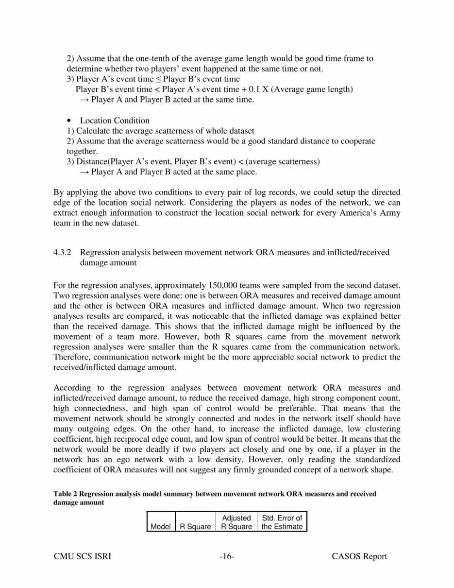
4.3.2 Regression analysis between movement network ORA measures and inflicted/received damage amount

For the regression analyses, approximately 150,000 teams were sampled from the second dataset. Two regression analyses were done: one is between ORA measures and received damage amount and the other is between ORA measures and inflicted damage amount. When two regression analyses results are compared, it was noticeable that the inflicted damage was explained better than the received damage. This shows that the inflicted damage might be influenced by the movement of a team more. However, both R squares came from the movement network regression analyses were smaller than the R squares came from the communication network. Therefore, communication network might be the more appreciable social network to predict the received/inflicted damage amount. According to the regression analyses between movement network ORA measures and inflicted/received damage amount, to reduce the received damage, high strong component count, high connectedness, and high span of control would be preferable. That means that the movement network should be strongly connected and nodes in the network itself should have many outgoing edges. On the other hand, to increase the inflicted damage, low clustering coefficient, high reciprocal edge count, and low span of control would be better. It means that the network would be more deadly if two players act closely and one by one, if a player in the network has an ego network with a low density. However, only reading the standardized coefficient of ORA measures will not suggest any firmly grounded concept of a network shape.

Table 2 Regression analysis model summary between movement network ORA measures and received damage amount

Model R Square Adjusted R Square

Std. Error of the Estimate


1 0.407 0.407 228.499

Table 3 Regression analysis model summary between movement network ORA measures and inflicted damage amount



1 0.453 0.453 222.731

4.3.3 Correspondence analysis with movement network ORA measures In this section we conducted a correspondence analysis on the movement network ORA measures of the top 1000 teams. The top 1000 teams are selected with the respect of each team’s new score introduced in the first technical report, and we consider the chosen top 1000 teams would be the most successful teams in the population. Before we did the correspondence analysis, we labeled the level of ORA measures with ‘H’, ‘M’, and ‘L’ representing ‘High’, ‘Medium’, and ‘Low’ respectively. The details about this labeling can be found in the first technical report. Also, the top 1000 teams are divided into 5 clusters, and these clusters are determined by K means analysis. After clustering and labeling, the number of instances for three levels of each ORA measures are counted for each cluster. Figure 8 shows the result of the correspondence analysis mapping 32 ORA measures and 5 clusters. It is noticeable that three out of five clusters are closely located, and it means that there are three actual clusters though we tried to make five clusters. Cluster 0, Cluster 2, and Cluster 4 have low in-degree centralization, low hierarchy, and high reciprocal edge count, and it suggests that those three clusters might have movement networks that have less centralized nodes, less hierarchical attributes, and many incoming/outgoing edges between two agents. Cluster 1 is located far away from the above three clusters and has medium in-degree centralization, medium diameter, and low connectedness. With the analysis result, we can expect that the movement networks of Cluster 1 might have more centralized nodes than the above three clusters have. Cluster 3 has high betweenness centralization and high total-degree centralization, and it makes the movement networks of Cluster 3 have more centralized nodes than any other clusters. Therefore, we can see that the majority of the top teams have less centralized agents and less hierarchical attributes and there are some top teams adopting more centralized movement network structure.


Figure 8. Correspondence analysis graph with 32 movement network ORA measures and 5 clusters

-1.5 -1.0 -0.5 0.0 0.5 1.0

-1.0

-0.5

0.0

0.5

1.0

1.5

2.0

Cluster 0

Cluster 1

Cluster 2

Cluster 3

Cluster 4

averagedistance.H

averagedistance.M

averagedistance.Laveragespeed.H

averagespeed.M

averagespeed.L

betw eennesscentralization.H

betw eennesscentralization.M

betw eennesscentralization.L

closenesscentralization.H

closenesscentralization.Mclosenesscentralization.L

clusteringcoefficient.H

clusteringcoefficient.L

connectedness.H

connectedness.L

density.L

diameter.H

diameter.Mefficiency.H

efficiency.L

hierarchy.H

hierarchy.M

hierarchy.L

indegreecentralization.H

indegreecentralization.M

indegreecentralization.L

interdependence.M

interdependence.L

lateraledgecount.H

lateraledgecount.L

minimumspeed.H

minimumspeed.L

netw orklevels.M

netw orklevels.L

outdegreecentralization.H

outdegreecentralization.M

outdegreecentralization.L

poolededgecount.H

poolededgecount.M

reciprocaledgecount.H

reciprocaledgecount.Msequentialedgecount.M

sequentialedgecount.L

skipededgecount.H

skipededgecount.L

spanofcontrol.L

strongcomponentcount.H

strongcomponentcount.M

strongcomponentcount.L

totaldegreecentralization.H

totaldegreecentralization.Mtotaldegreecentralization.L

transitivity.H

transitivity.L

upperboundedness.M

upperboundedness.L

w eakcomponentcount.M

w eakcomponentcount.L

know ledgediversity.Hknow ledgeload.M

know ledgeredundancy.H

know ledgeredundancy.M

know ledgeredundancy.L

accessredundancy.H

accessredundancy.M

accessredundancy.L

resourcediversity.H

resourcediversity.M

resourcediversity.L

resourceload.H

resourceload.M

resourceload.L


4.4 Social network approach based on ‘who-talked-after-whom’ network

4.4.1 How to construct ‘who-talked-after-whom’ network ‘Who-talked-after-whom’ social network has been analyzed since the first tech report of America’s Army. Because every transmitted communication message is received by all the squad members, there was no way to extract the edges linking two players. Therefore, ‘Who-talked-after-whom’ heuristic is introduced. The basic idea of the heuristic is the person who talked after the other person is responding the previous message, so we can get edges based on this assumption. The more detailed information can be found in the previous tech report. Figure 9 describes the process of converting log records to the ‘who-talked-after-whom’ network.

Figure 9. How-to construct who-talked-after-whom network with the sequence of communication messages

��

� �

� �

� �

� �

� �

� �

�

��

��

��

��

��

��

��

4.4.2 Regression analysis between communication network ORA measures and inflicted/received damage amount

With about randomly selected 150,000 teams, two regression analyses were done between ORA measures and received/inflicted damage amount. Two regression analyses are almost same to the two regression analyses in the previous sub-chapter except we used ORA measures came from the communication network for this time. Compared to the previous pair of regression analyses with the movement network, the regression analyses with the communication network show higher R squares, and it means that the communication network might be the better input for predicting received/inflicted damage amount. Also, like the previous analyses, the inflicted damage amount is explained better than the received damage amount. Therefore, it seems that the social network of a team affects more on the inflicted damage amount rather than the received damage amount. When we observe the standardized coefficients of the regression analyses between communication network ORA measures and inflicted/received damage amount, we can conclude that high average speed, low weak component count, and low reciprocal edge count will reduce


the received damage amount. On the other hand, low average distance, low density, and high span of control would be better in increasing the inflicted damage amount. Also, this result suggests us to make sparse communication network instead of the dense communication network. However, it is true that there are other variables with strong standardized coefficients, so we cannot simply make the recommended shape of a communication network.

Table 4 Regression analysis model summary between communication network ORA measures and received damage amount



1 0.411 0.411 227.675

Table 5 Regression analysis model summary between communication network ORA measures and inflicted damage amount



1 0.493 0.493 214.483

4.4.3 Correspondence analysis with communication network ORA measures Figure 10 presents the result of the correspondence analysis mapping 32 communication network ORA measures and 5 clusters. There is no clear correlation between 5 clusters like the previous correspondence analysis on the movement network, and it means that all of the 5 clusters have their own structures. Cluster 0, Cluster 1, and Cluster 3 have relatively high density when they are compared to Cluster 2 and Cluster 4. Cluster 2 has medium level of sequential edge count unlike Cluster 1 and Cluster 3 having low sequential edge count. Cluster 4 has low skipped edge count compared to the rest of Clusters. However, it should be noted that we cannot make any hard recommendations based on the correspondence analysis because guessing the network structure with the levels of ORA measures is very difficult. Therefore we invented ‘Network Fitter’ to visualize the typical network structure for each cluster.


Figure 10. Correspondence analysis graph with 32 communication network ORA measures and 5 clusters

-2 -1 0 1 2

-1.5

-1.0

-0.5

0.0

0.5

1.0

1.5

Cluster 0

Cluster 1

Cluster 2

Cluster 3

Cluster 4

averagedistance.M

averagedistance.L

averagespeed.M

averagespeed.L

betw eennesscentralization.M

betw eennesscentralization.L

closenesscentralization.H

closenesscentralization.M

closenesscentralization.L

clusteringcoefficient.H

clusteringcoefficient.M

clusteringcoefficient.L

connectedness.Hconnectedness.M

density.H

density.M

density.L

diameter.H

diameter.M

diameter.Leff iciency.H

efficiency.M

efficiency.L

hierarchy.H

hierarchy.Lindegreecentralization.H indegreecentralization.M

indegreecentralization.L

interdependence.H

interdependence.M

interdependence.L

lateraledgecount.M

lateraledgecount.L

minimumspeed.H

minimumspeed.M

minimumspeed.Lnetw orklevels.H

netw orklevels.M

netw orklevels.L

outdegreecentralization.H

outdegreecentralization.Moutdegreecentralization.L

poolededgecount.H

poolededgecount.M

poolededgecount.L

reciprocaledgecount.H

reciprocaledgecount.M

reciprocaledgecount.L

sequentialedgecount.H

sequentialedgecount.M

sequentialedgecount.Lskipededgecount.H

skipededgecount.M

skipededgecount.L

spanofcontrol.M

spanofcontrol.L

strongcomponentcount.H

strongcomponentcount.Mstrongcomponentcount.L

totaldegreecentralization.H

totaldegreecentralization.M

totaldegreecentralization.L

transitivity.H

transitivity.M

transitivity.L

upperboundedness.M

w eakcomponentcount.M

w eakcomponentcount.L

know ledgediversity.Hknow ledgeload.M

know ledgeload.L

know ledgeredundancy.H

know ledgeredundancy.M

know ledgeredundancy.Laccessredundancy.H

accessredundancy.M

accessredundancy.Lresourcediversity.H

resourcediversity.M

resourcediversity.L

resourceload.H

resourceload.M

resourceload.L


4.5 Statistical analysis with team variables

4.5.1 Regression analyses with team variables against performance measures So far, regression analyses were done between ORA measures and the amount of the inflicted/received damage. Either movement social network or communication social network is used, not both networks at the same time. For this chapter, we will utilize the same regression analysis with more explanatory variables that came from general calculation like clanishness, the number of comm., etc. Moreover, we will use ORA measures obtained from the two social networks at the same time. We will use 150,000 team instances for this time. For the dependent variables of the regression analyses, we used four performance measures: inflicted damage amount, received damage amount, winning and new score. First, we did a regression analysis with the whole explanatory variables against the inflicted amount of damage. Compared to the previous regression analysis that only used ORA measures calculated from one type of social network, R square is greatly improved, from 0.45~0.49 to 0.55. It is certain that the other factors except social network measures effects greatly on the performance measure. Movement network density (Beta coef.: 0.279), movement network span of control (-0.285), number of Report-In (0.172) have high beta coefficient values and can be considered significant factors affecting the amount of the inflicted damage. It is quite noticeable that adding more variables improves R square but still ORA measures have high standardized coefficient values. Thus, we may guess that organizing social networks would be important to increase the inflicted damage amount.

Table 6 Summary of the regression analysis: whole team level measures against the inflicted damage amount

Model R

Square

Adjusted R

Square

Std. Error of the

Estimate 1 0.55 0.549 202.21238

Second, we conducted a regression analysis against the received damage amount. The R square of the regression against received damage is not as good as that of regression against inflicted damage. However, still the R square is reasonably good, 0.499. Surely, R square is improved compared to the previous analysis that used only ORA measures of individual social network (either movement or communication). Number of total communication (Beta coef.: 0.785), number of Report-In (-0.48), communication network knowledge redundancy (0.468) are the significant variables in terms of beta coefficient. Unlike the inflicted damage regression, communication related measures are highly regarded, and it tells us that communication is more important in reducing the amount of damage.

Table 7 Summary of the regression analysis: whole team level measures against the received damage amount

Model R

Square

Adjusted R

Square

Std. Error of the

Estimate


1 0.499 0.499 209.92397 Third, a regression analysis with the team level measures against winning is done. For the dependent variable value, we set the winning case is one and the losing case is zero. Though the R square is not good, but it is improved. However, we should consider that the winning variable is just a binary variable, so it will be hard to fit in the regression model. Though the R square is low, we can use the beta coefficient to get insights about factors affecting winning. Three communication measures, number of total communication (-0.543), number of Report-In (0.459), number of Commo. (A short message like ‘move’, ’roger’, 0.271), are very highly ranked among the explanatory variables. The regression shows that the communication is very important in winning the game. Also, being deadly, being invulnerable, and being successful require different factors according to the regression analyses.

Table 8 Summary of the regression analysis: whole team level measures against the winning

Model R

Square

Adjusted R

Square

Std. Error of

the Estimate

1 0.138 0.138 0.461 Finally, a regression against the new score is conducted. The new score is better in the fitting compared to the winning variable, but it has lower R square compared to the regression against the inflicted/received damage. It suggests that using the actual amount of damage might be good for analysis of regression, but still we need a regression analysis with a unified measure to get a general idea about team success. Levels of communication measures are very important, and it is true because the new score takes inputs from the original scores that are largely influenced by winning. Therefore, the measures having great influence on winning also affect greatly on the new score.

Table 9 Summary of the regression analysis: whole team level measures against the new score

Model R

Square

Adjusted R

Square

Std. Error of the

Estimate 1 0.188 0.188 148.94017

When we review the four regression analyses that take inputs from the team measures and fit into the four performance variables, R square is improved when we compare it to the regression that used only one type of social network ORA measures. Predicting the inflicted/received damage amount is really well explained by the regressions (above 0.5 R square values). The inflicted amount of damage relies on the movement network measures (like movement network density or span of control), but the other performance measures are largely influenced by the level of communication. We could identify that the level of communication and the ORA measures are important factors in predicting a team performance. Appendix C contains the more detailed statistic analysis result such as beta coefficient, significance level, etc.


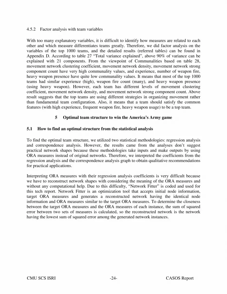
4.5.2 Factor analysis with team variables With too many explanatory variables, it is difficult to identify how measures are related to each other and which measure differentiates teams greatly. Therefore, we did factor analysis on the variables of the top 1000 teams, and the detailed results (referred tables) can be found in Appendix D. According to table 27 “Total variance explained”, above 90% of variance can be explained with 21 components. From the viewpoint of Communalities based on table 28, movement network clustering coefficient, movement network density, movement network strong component count have very high communality values, and experience, number of weapon fire, heavy weapon presence have quite low communality values. It means that most of the top 1000 teams had similar experience (high), weapon fire count (many), and heavy weapon presence (using heavy weapon). However, each team has different levels of movement clustering coefficient, movement network density, and movement network strong component count. Above result suggests that the top teams are using different strategies in organizing movement rather than fundamental team configuration. Also, it means that a team should satisfy the common features (with high experience, frequent weapon fire, heavy weapon usage) to be a top team.

5 Optimal team structure to win the America’s Army game 5.1 How to find an optimal structure from the statistical analysis To find the optimal team structure, we utilized two statistical methodologies: regression analysis and correspondence analysis. However, the results came from the analyses don’t suggest practical network shapes because these methodologies take inputs and make outputs by using ORA measures instead of original networks. Therefore, we interpreted the coefficients from the regression analysis and the correspondence analysis graph to obtain qualitative recommendations for practical applications. Interpreting ORA measures with their regression analysis coefficients is very difficult because we have to reconstruct network shapes with considering the meaning of the ORA measures and without any computational help. Due to this difficulty, “Network Fitter” is coded and used for this tech report. Network Fitter is an optimization tool that accepts initial node information, target ORA measures and generates a reconstructed network having the identical node information and ORA measures similar to the target ORA measures. To determine the closeness between the target ORA measures and the ORA measures of each instance, the sum of squared error between two sets of measures is calculated, so the reconstructed network is the network having the lowest sum of squared error among the generated network instances.


Figure 11 How the network fitter works and what it can do

Because our goal of this chapter is generating the optimal shape of a social network, we coded the initial node information of a squad-level network that resembles to the 10-man team. After coding the node information, we applied Network Fitter to the node information with the averaged ORA measures of each cluster in the top 1000 teams. As a result, for each network type, we could obtain five suggested network shapes corresponding to the five clusters in the top 1000 teams. 5.2 Optimal team movement structure As we conducted the correspondence analysis, we used the five clusters determined by the k-means analysis to make the five corresponding optimal team structures. After making the optimal team structures, we calculated some measures representing the characteristics of the teams in the clusters. The average measured values for each cluster are divided by the average values for the entire top 1000 teams, so we could compare the cluster specific measure value to the average of the top 1000 teams. Considering the five generated optimal movement network structure, we could identify there are three types of distinct network structures among the top 1000 teams. The three optimal structures are Dense Movement Network (Moving together), Sparse Movement Network (One fire-team and several isolated players), and Disconnected Movement Network (Keeping distance to each other). Table 10 illustrates how many top teams have a certain movement network type. It says that the disconnected movement network is the majority, but cluster1 that have a dense network is the majority when we considers only well connected networks. At the following sub chapters, we discuss the distinct characteristics for each movement network shape with two types of figures: one for a certain network shape and one for comparison between teams adopting the network shape and the entire top 1000 teams.

Table 10 Number of teams classified into each movement network clusters

Moving together One fire-team Keeping distance to


and several isolated players

each other

Cluster 1 Cluster 3 Cluster 5 Cluster 4 Cluster 2 Cluster Num. 252 65 17 198 508

5.2.1 Dense movement structures: Moving together Cluster 1, 3, and 5 show somewhat similar movement network structures and the similarity is already identified by the correspondence analysis in the previous chapter. The overall movement network shapes of those clusters are very dense, so their scatterness is much lower than the average of the top 1000 teams. Particularly, the clannishness measures of cluster 3 and 5 are lower than the average, so it seems that the members of the teams move together very closely because the team members didn’t know what the other members do. Especially, cluster 1 should be noted due to its uniqueness of the structure and performance. Cluster 1 has low casualty and slightly low received damage, and it has somewhat low communication frequency which reduce team members’ communication burden though they are communicating a lot than the ordinary teams. Moreover, cluster 1 movement network is good for reducing the number of normal communication messages because cluster 2 and cluster 4 have high frequency in the normal communication. Reducing the normal communication message allows players to concentrate on shooting, movement and achieving objectives. Cluster 1 also has lower number of shooting compared to the other top 1000 teams, and it is good because they are spending less ammos and still very good. Finally, cluster 1 has the lowest game length, and it means that the teams of cluster 1 won in very short time. Some of these good characteristics are so unique that even the other similar networks like cluster 3 or cluster 5 don’t have such attributes. We conjecture the benefits of cluster 1 movement network came from its distinct movement network shape that is different to the other dense movement networks. Cluster 1’s movement network structure has two distinct leaders and those leaders have connections to the rest of members, and this rational fits the two fire team structures. When we did the clique analysis of the network, we could see that two sub graphs exist in the network. On the other hand, the other two dense movement network did not show multiple sub graphs, but only one strongly connected network with the sub graph analysis.


Figure 12 Dense optimal movement network structures (Left) and their descriptive measures (Right)

5.2.2 Sparse movement structures: One fire-team and several isolated players Cluster 4 has medium density among the optimal movement networks. The optimal network for the cluster 4 shows one connected networks and five isolated nodes, and we think the connected


network represents one fire team and the isolated nodes shows the individually moving players. This movement network is not typical because it has high scatterness and individually acting players. However, it has high clanishness measures compared to the clusters having dense movement network, so we guess that the isolated players are doing actions already coordinated. Because they are dispersed, the frequency of communication tends to increase, so the number of Report-In is high. The number of normal communication is also high, and it is unusual for a team having high clanishness. To wrap up, the teams of cluster 4 have high clanishness compared to the teams having dense movement network, high communication frequency in both Report-In and normal communication, and high scatterness. We think these teams already assigned detailed tasks to each player, some of highly skilled team members do their tasks individually, the other players form a fire team and fight against the enemy, and they communicate very frequently.

Figure 13 A sparse optimal movement network structure (Left) and its descriptive measures (Right)

5.2.3 No movement structures: Keeping distance to each other Cluster 2 has an extremely sparse movement network, and it means the team members were scattered and did not stay close together in the virtual space. This is awkward according to the previous research that stated winning teams have lower scatterness. However, this sparse movement network is the majority among the top 1000 teams, so we conjecture that there are two types of teams among the top 1000 teams: well-organized teams and teams with excellent players. We guess that the well-organized teams usually adopt the previous movement networks, and the teams with excellent players organize the movement network with very low density in the network. This sparse movement network might not be a good recommendation because there is no guarantee that a squad will always have excellent and experienced soldiers.


Figure 14 An extremely sparse optimal movement network structure (Left) and its descriptive measures (Right)

5.3 Optimal team communication structure We conducted the same analysis on five communication network clusters. These network clusters come from the top 1000 teams similar to the previous analysis. The five presented agent to agent networks are the optimal communication network structures corresponding to five clusters, and the bar graphs are the comparisons between the average measures of each cluster and those of the overall top teams. With the five generated optimal communication network structure, we could capture two distinct communication network types: a long chain-shaped communication network and a star-shaped communication network. Among the top 1000 teams, there are slightly more teams adopting a long chain-shaped communication network, but the number of the top teams adopting the other communication network is also significant. Table 11 suggests the number of the top teams categorized into a certain cluster and the number of the top teams adopting a suggested optimal communication network. Unlike the previous optimal team structure analysis on the movement network, all the five suggested communication network have quite reasonably dense communication network, and it suggests that the top teams keep communicating each other even though they sometimes utilize quite unorganized movement network structures. Furthermore, the emphasis of the communication networks in terms of the network density reminds us the importance of communication.

Table 11 Number of teams classified into each communication network clusters

Long chain-shaped Communication

Network Star-shaped Communication

Network Cluster 1 Cluster 5 Cluster 2 Cluster 3 Cluster 4

Cluster Num. 265 254 23 335 123


5.3.1 Dense communication structure: Star-shaped communication structure Cluster 2, 3 and 4 have slightly denser communication networks than the other clusters have, but the casualties of those clusters are higher than the other networks. It means that they are quite vulnerable from the attack. At the same time, they have higher inflicted damage, so the teams adopting star-shaped communication networks seems to be more aggressive and more vulnerable. For example, it should be noted that the cluster 2 has very high casualty while it has higher communication frequencies across all types of communication. It means that only increasing number of communication would not improve the survival rate of a team. The communication network should be efficient, so it can exchange information well with fewer communication messages. Furthermore, cluster 2 and 4 have very high frequency in normal communication, and it is not that recommendable because it takes time to type in such a message. Cluster 3 is an eccentric cluster among the clusters using the star shaped communication network. It seems that cluster 3 has less dense communication network compared to the other star shaped communication network, so the slight difference in the topology or the number of communication links might changes the performance of teams of cluster 3.

Figure 15 Three optimal communication network structures (Left) and their descriptive measures (Right)


5.3.2 Sparse communication structure: Long chain-shaped communication structure Cluster 5 has the typical long-chain shaped communication network, and cluster 1 has little similar structure compared to cluster 5. Because the long-chain communication network does not require many communication messages, the cluster has lower frequency of communication. However, the casualty and the received damage are low, and it means that the communication network was quite efficient in terms of survival rate. At the same time, the number of killed opponent players and the amount of inflicted damage are the average level of the top 1000 teams, so they are still deadly enough to be nominated among the top 1000 teams. This communication network shape may not be the best choice in a certain situation like maximizing the deadliness of a team because the clusters with star-shaped communication networks have slightly higher number of killed opponent, but the long-chain shaped communication network ensures the safety of a team by reducing the number of communication messages and by organizing the communication network efficiently. Particularly, we can observe that the communication network structure of cluster 5 has very small number of normal communication messages, and it helps team members to focus on the other tasks and team to win in short time length.

Figure 16 Two optimal communication network structures (Left) and their descriptive measures (Right)


6 Practical recommendations for training and configuring squad level military unit 6.1 Similarities and differences between America’s Army and real world

6.1.1 Comparison between America’s Army and real world research To remind the comparison between America’s Army and real world research, Table 12 is presented. After the statistical analyses of the first tech report, we could identify some similarities between them. The high performance team size, 10-men team size, was identical in both domains. Also, the importance of fire volume and Report-In was found in both domains. Because many recommendations and detailed statistical analyses were made based on the importance of them, the fact that fire volume and Report-In are important in both domains is very valuable in validating the recommendations and analyses.

Table 12.The summary of comparisons between America's Army and the squad-level real world research

America’s Army Real world

Team configuration High survival rate of 10-player teams

10-men infantry rifle squad of Reorganization Objective Army Division (ROAD) [7]

Weapon usage Importance of Heavy weapon

Soldiers with heavy weapons are very effective [7]

Communication usage Importance of Report-In communication

Importance of Provide (friendly) information communication [8]

6.1.2 Comparison between America’s Army and Command and Control experiments In previous tech report, Command and Control (C2) experiments [9] are compared to the America’s Army game. For the brief recall of the comparison, Table 13 is made. First of all, it


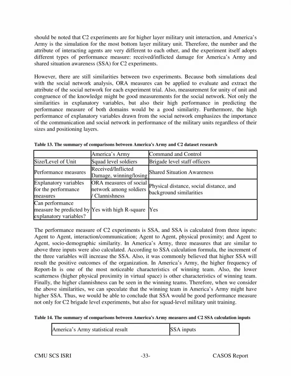
should be noted that C2 experiments are for higher layer military unit interaction, and America’s Army is the simulation for the most bottom layer military unit. Therefore, the number and the attribute of interacting agents are very different to each other, and the experiment itself adopts different types of performance measure: received/inflicted damage for America’s Army and shared situation awareness (SSA) for C2 experiments. However, there are still similarities between two experiments. Because both simulations deal with the social network analysis, ORA measures can be applied to evaluate and extract the attribute of the social network for each experiment trial. Also, measurement for unity of unit and congruence of the knowledge might be good measurements for the social network. Not only the similarities in explanatory variables, but also their high performance in predicting the performance measure of both domains would be a good similarity. Furthermore, the high performance of explanatory variables drawn from the social network emphasizes the importance of the communication and social network in performance of the military units regardless of their sizes and positioning layers.

Table 13. The summary of comparisons between America's Army and C2 dataset research

America’s Army Command and Control Size/Level of Unit Squad level soldiers Brigade level staff officers

Performance measures Received/Inflicted Damage, winning/losing Shared Situation Awareness

Explanatory variables for the performance measures

ORA measures of social network among soldiers / Clannishness

Physical distance, social distance, and background similarities

Can performance measure be predicted by explanatory variables?

Yes with high R-square Yes

The performance measure of C2 experiments is SSA, and SSA is calculated from three inputs: Agent to Agent, interaction/communication; Agent to Agent, physical proximity; and Agent to Agent, socio-demographic similarity. In America’s Army, three measures that are similar to above three inputs were also calculated. According to SSA calculation formula, the increment of the three variables will increase the SSA. Also, it was commonly believed that higher SSA will result the positive outcomes of the organization. In America’s Army, the higher frequency of Report-In is one of the most noticeable characteristics of winning team. Also, the lower scatterness (higher physical proximity in virtual space) is other characteristics of winning team. Finally, the higher clannishness can be seen in the winning teams. Therefore, when we consider the above similarities, we can speculate that the winning team in America’s Army might have higher SSA. Thus, we would be able to conclude that SSA would be good performance measure not only for C2 brigade level experiments, but also for squad-level military unit training.

Table 14. The summary of comparisons between America's Army measures and C2 SSA calculation inputs

America’s Army statistical result SSA inputs


Number of communication (Number of Report-In) interaction/communication

Scatterness physical proximity Clannishness socio-demographic similarity

6.2 Guidelines to win America’s Army game from the previous and the current tech

report By writing the first and the second tech report, we tried to identify winning strategies at player, team, and clan level. Of course it is very hard to say that certain aspects or methodologies are the strategies of winning team, so we assumes that the tendencies resulted from the statistical analyses of winners would be the winning strategies. Following subsections summarize the important findings with itemized phrases. More detailed implications can be found at Chapter 6.3, 6.4, and 6.5.

6.2.1 Strategies for players

• Handle various weapons: from M4, M16, AK47 rifles to M9 pistol and SPR,SVD sniper rifle

• Transmit Report-In communications as many times as possible • Do seeking covers and firing weapons to enemy at the same time • Keep selecting the medic role if you want to be a medic • Ambushing enemy is better than rushing to enemy

6.2.2 Strategies for teams

• Be consisted of 10 players to maximize the survival rate • Equip two or more fire team members with heavy weapons • Overwhelm the enemy in the fire volume • Report-In communication is the most important messages for team success. • When a player transmits a Report-In, the other players should respond one by one, and

this chain of Report-In should connect as many team members as possible. • Even though the team is very experienced and play games together very often, it would

be recommendable to keep transmitting a lot of Report-In during the play. • Players should not be dispersed across the game play space. • Both winning teams and losing teams should cover almost same number of spots on game

field, but winning team members always stay close to the other team members who are at the same spot (fire team members).

6.2.3 Strategies for clans

• Making a team with same clan members is the most effective way to win.


• Play together very often to be familiar with the other clan members’ play styles. • Forming a team with players who are participating in clans is the alternative way to win

because players who are in clans would have better knowledge and experience than the ordinary players have, but this is not as good as playing with same clan members because they don’t know how to coordinate game play due to the lack of understanding each other’s play.

6.3 Recommendation on training squad level military unit

6.3.1 Recommendation at soldier level Top players in America’s Army show some distinct traits in their game play. They tend to plan their role selection from the beginning, play with extreme caution, utilize the communication greatly, and know the characteristics of weapons. From the found traits, we made recommendations on training soldiers from the viewpoints of individual movement, equipment, communication, and carrier selection. � Train soldiers to fire their weapons and to seek covers at the same time

: Top players of America’s Army don’t get damage although they become more aggressive. They have an ability that makes them deadly and invulnerable at the same time. Therefore, the soldiers should be trained to move and shoot their weapons at the same time.

� Train soldiers to transmit Report-In frequently

: It is obvious that transmitting Report-In many times is the key to win the combat. This can help the other team members aware where their friendly forces are. There might be incidents that friendly forces shot each other and some soldiers were isolated without notice. By training soldiers to transmit Report-In many times, these unwanted situations will be avoided.

� Train soldiers to handle heavy weapons

: Heavy weapons are important and critical resources on America’s Army battlefield. Sniper rifles, automatic rifles, and rockets can suppress the enemy and support the friendly forces. Also, in real world, many incidents were reported that numerous soldiers were suppressed by one sniper or one automatic rifle. Equipping more soldiers with heavy weapon might be the way to improve squad units.

� Train soldiers not to rush, but to ambush

: Ambushing is the conspicuous tactic the top players adopt. It can be done in any place: room, air condition venue, roof, etc. Also, it is critical for soldiers not to rush into such places where enemy can easily ambush. This recommendation implies that the combat soldiers should be more patient and cautious.

� Train medics from the beginning of their training

: Among the top players of America’s Army, there are medic specialized top players, and they keep choosing medic role. By training them from the beginning, soldiers will know


what to do as a medic. In America’s Army game, medic specialized top players transmit Report-In a lot, concentrate treating the other team members rather than fighting against enemies, and understand they should not be shot because it would be fatal.

6.3.2 Recommendation at squad level Teamwork would be the most important feature in the success of a team, and we could identify some guidelines that can enhance the teamwork of America’s Army team. Although a team consists of good players, they have to cooperate to each other to achieve the winning. Therefore, the guidelines to enhance the teamwork should be the guidelines to increase the chance of cooperation. We present several points that can maximize the cooperation. � Train soldiers to move with their fire team members closely

: Winning teams and losing teams of America’s Army have almost same number of groups whose group members move together. However, the winning teams’ small groups are more centered, and the winning players who belong to the small group stay closer to the other players who are in the same small group than the losing players do. Therefore, if we consider the small group as a fire team, soldiers should be trained to stay close to their fire team members.

� Train soldiers to make a chain of Report-In communication

: The best communication network structure in America’s Army game is the long chain shaped communication network. All squad members should remember the squad member who will Report-In next to them. When the squad leader starts Report-In, the squad members should respond by transmitting Report-In in the predefined order. If the next soldier who is supposed to Report-In has not responded, the soldier after that should report in. The squad leader should not have to remind him and distract the squad leader from his other duties.

� Train soldiers to transmit Report-In particularly frequently during the middle of combat

: This can be done by training squad leaders to transmit Report-In a lot during the middle of combat because the other squad members should be trained to respond the squad leader’s Report-In.

� Train soldiers to fire their weapon a lot

: Each soldier might have small fire volume if the soldier has a sniper rifle. However, the overall squad should overwhelm the opponent by firing their weapons very frequently. Therefore, the soldier with Squad Automatic Weapon (SAW) and the soldier with the sniper rifle should cooperate closely with each other.

6.3.3 Recommendation at unit level Clans in the America’s Army community can be considered units that are higher level of squad units. During the analyses, we could identify the distinctive attribute of winning teams, and the


attribute can be controlled at the clan level. Thus, it might be possible to upgrade the capability of a squad by training and configuring it with some unit level guidelines. � Train soldiers to know their teammates’ combat style

: Being in the same unit lets soldiers be familiar with their teammates’ combat style. This is very important because team members can reduce the verbal communication in real situations and concentrate on more valuable and meaningful communication like Report-In by knowing their teammates’ combat style.

� Don’t deploy soldiers trained in separate units as one squad

: They are not familiar with the other squad members’ combat style. In this case, their verbal communication increases and their time will be spent less efficiently in real world situations.

6.4 Recommendation on Tactics, Techniques, and Procedures at squad level Tactics, Techniques, and Procedures (TTP) for Squad level radio communication was defined by Redden and Blackwell [10], 2001. It describes the procedures and rules for requesting and transmitting messages at squad level radio communication. So far, ARL research defined 5 TTPs, and they were utilized in the field experiments to evaluate its performance. The ARL defined TTPs emphasize the hierarchical command level, so the squad leader (SL) and two team leaders (TL) are the main contact node of the communication. The 5 TTPs can be seen in Table 15. According to the descriptions of TTPs and fundamental assumptions of ARL research, we can find some common aspects among TTPs. � The SL can always transmit messages to anyone in his squad at any time. � Everyone can always listen to squad radio transmissions. � Everyone can use hand and arm signals at any time. � If a TTP allows you to transmit, use the squad radio as your primary means of verbal

communication � If a TTP forbids you to transmit and you need to say something out loud, communicate

the way you normally would without a squad radio

Table 15 5 TTPs defined by ARL research

TTP Name Description TTP 1 Don’t Talk Team leaders and team members (TM) cannot transmit. TTP 2 TL to SL Only TLs can transmit at any time, but only to SL. The TMs cannot

transmit. TTP 3 When SL Asks TLs and TMs cannot transmit, unless the SL asks them to transmit to

him. TLs and TMs cannot transmit again until the SL asks them to transmit to him again.

TTP 4 Up and Down TLs can transmit to their TMs and to the SL at any time. The TMs can transmit to their TL or to the SL at any time.

TTP 5 Free Talk TLs and TMs can transmit to anyone in the squad at any time (including TL to TL and TMs to TMs in other teams).


However, in some perspectives, these TTPs are questionable. For example, what if an emergent situation happened, should squad members (SM) get permission to speak from their superior? According to the above tables and assumptions, SMs have no way but to wait SL asks questions, send information through TL, or shout the information loudly, and these solutions would not be very good idea in some situations. Also, we conjecture that the entire SMs should operate together even though there are two separate fire teams because the squad is a small military unit. However, the suggested TTPs are quite strict in terms of hierarchical structure between fire teams and squad leaders. There are not that obvious ways to communicate SMs who are in different fire teams. Of course, TTP5 grants unlimited communication privileges to SMs, but it lacks discipline that is crucial when number of soldiers communicate on one communication frequency. To understand the ARL suggested TTPs and our recommended TTP, let’s consider the following hypothetical case. If there are three squad members (B, C, and D) and one squad leader (A), the star shaped communication network might be the left network on Figure 17. Also, the long chain shaped communication network would be the right network.

Figure 17 Diagram describing how the star shaped communication network and the long chain shaped communication network work

Because ARL research is strict on the command hierarchy and tries to apply the command hierarchy to the communication TTP, the star shaped communication network might be the abstract version of communication network that can be generated by ARL recommended TTPs. On the other hand, the long chain shaped communication network is the network we discovered with the result of data-mining of the top 1000 teams communication network. Therefore, we first extracted desirable communication network from the America’s Army top teams and rebuild an appropriate TTP that enables the long chain shaped communication network. Our TTP is “Sequential transmit”: when the SL transmits the other SMs transmit, one by one, followed by previously defined order. Star shaped communication network would be better if the leader can transmit many messages at the same time, but we are talking about single band squad radio communication. If a squad adopts the star shaped communication network, every time the SL asks, the SL will get only information from single SM. On the contrary, chain shaped communication network would be better if every member remembers their orders to send out communication message in squad

A

C B D

A

C B D

Star shaped comm. Network Commonly adopted by ARL TTPs

Newly proposed TTP Identified from the Report-In comm. Network

analysis of top America’s Army teams

A ask � B answer � A ask � C answer � A ask � D answer

A transmit � B transmit � C transmit � D transmit


radio communication. In that case, every time leader asks, the chain will be activated, and the information will flow through all the squad members. If we understand the distinctive attributes of squad level radio communication, it will be easier to understand the pros and cons of each communication network topology. To know the attributes of the squad level radio communication, we compared brigade command and control (C2) level communication, upper layer military unit communication, to squad level communication, bottom layer military unit communication.

• At brigade level C2 communication : There are multiple computers, communication devices, and communication frequencies. Each communication node consists of a number of officers, so each node can deal with multiple incoming/outgoing transmissions. They are not directly involved in combat as squad level soldiers are.

• At squad level radio communication : One small radio is the only resource each soldier has for communication. Each soldier has to fire weapons, change positions, and communicate the other members at the same time. Extremely dynamic, so information should flow very automatically.

When we examine the above situation, we might conclude the chain shaped communication network would be better. The SL of a squad can gather information by making one report-in request. The Report-In information will flow through every single team members. Each team member only has to focus on their previous Report-In member. This way is very effective when there are many tasks that the SL should do with time and resource constraint. If the SL always has to ask where SMs are individually, it would be impossible to manage the whole squad. Also, if the communication is disconnected between two fire teams, there will be missing opportunity that two fire teams can cooperate together and be successful. This long chain shaped communication network and its corresponding TTP is very autonomous started by one request from the SL and covers all the SMs regardless of the fire team composition. 6.5 Recommendation on configuring the squad level military unit Figure 18 shows the typical squad-level infantry unit composition. It specifies the size of a squad, the hierarchy of command, and the weapon equipment. This Reorganization Objective Army Division (ROAD) recommended squad structure was adopted in early 1960’s, but it was rejected soon due to the unbalanced sizes of two fire teams [7]. This diagram was introduced in this tech report because it resembles to our suggested squad structure. However, this ROAD recommended squad structure presents no information about how to move and how to communicate. It seems that this structure simply assumes every activity will be done with same fire team members.


Figure 18. The composition of squad-level infantry unit according to the ROAD recommendation

After the data analyses of two datasets from the America’s Army game, we could capture the important characteristics of winning teams and suggest the corresponding recommendations for configuring squad structure and training. We summarized some of those recommendations in one diagram showing the recommended squad-level structure. First of all, we specified the chain of communications with white arrows. Because we concluded the long chain shaped communication network structure would be good, the white arrows showing the communication network covers all of the squad members and shaped like a long chain. Also, we specified the two fire teams, and the members of a fire team should stay close to their same team members during the combat. Due to the importance of the heavy weapon, we added two soldiers with sniper rifles and one soldier with RPG instead of three soldiers with ordinary rifles.

Figure 19. The composition of the squad-level unit according to the result of the America's Army data analysis


7 Conclusion We conducted the second data analysis with a new game log record dataset. Unlike the previous dataset, the new one includes the location information of each game event, so we could analyze the team organization and behavior from the viewpoint of movement of players or teams. Because we did numerous statistical analyses at player level and clan level in the first tech report, we focused on the team organization in terms of movement and communication at team level. To find more effective team organization, we utilized regression analyses and correspondence analyses. However, with only those statistical analyses, we was not able to make a recommendable team organization structure, so we coded ‘Network Fitter’ and used it to make a computer program figure out the most effective team organization. After identifying the optimal movement networks and the communication networks, we applied the findings from the analyses to the real world and made three recommendations on training squad level unit, constructing effective TTP, and configuring an optimal squad unit. Before we did the major statistical analyses, we verified the second dataset shows the same tendencies found from the first tech report. With the simple calculation of communication frequency and survival ratio, we could confirm that the Report-In communication does important roles in teams’ success and the 10-man team structure has relatively high survival rate. Because we confirmed the above two aspects, we used Report-In communication network to build the teams’ communication network and made a recommended team structure having 10 players. Also, the location information had been analyzed with preliminary statistical analyses. We calculated the average standard deviation of three coordinates, the scatterness, the movement distance, and the average distance from the cluster centers determined by the k-means analysis on the game events. Those analyses agree that the team members should be located closely to the other team members and the physically scattered teams do worse in the games. Based on this result, we could identify that the relative location of team members affect to the team’s success and determined to analyze the movement network furthermore. From the regression analyses and correspondence analyses, we could capture a somewhat vague optimal network structure. The resulted network structure was not exact because we had to make a network structure based on the coefficients or graphs generated by those analyses. Furthermore, the R square value of the regressions was not quite impressive. From the correspondence analyses, we could capture how the 1000 teams can be categorized into five clusters and what the characteristics of each cluster are. However, due to the difficulty of the interpretation of ORA measures and the reconstruction of networks, we rather addressed the problem with the network fitter. With K-means analysis, all of the top 1000 teams were categorized into five clusters in terms of movement and communications. After the clustering, we utilized the network fitter and obtained the five optimal team structures corresponding to the five clusters. This allowed us to capture the five optimal movement networks and the five communication networks. Among the five optimal movement networks, there were largely two types of networks: dense network and sparse network. The dense networks suggest that the team members stay together very closely. Among the dense networks, the network with two sub groups has fewer casualties and communications than others but a satisfying number of killed opponent. Hence, that team might be better off if it


were to organize two fire teams and locate fire team members together. We used the same analysis technique on the communication networks, and found two dominant communication network types: star shaped communication network and long-chain shaped communication network. However, the long chain shaped communication network performed better than the other networks because the teams with the communication network has fewer casualties, less communication, and yet sufficient inflicted damage. Particularly, the lower communication frequency is important as it reduce team members’ burden to communicate, but it should be emphasized that the reduced communication frequency of the long-chain shaped communication network teams is still higher than that of losing teams. Based on the above analyses, we qualitatively analyzed the relation between the real world and America’s Army and made recommendations to real world. We compared the features of America’s Army and those of real world squad level research papers. Also, we compared America’s Army data analysis to the C2 experiment analysis. By doing these qualitative comparisons, we could see there are number of similarities. Because we found some similarities between America’s Army and the real world, we made three recommendations to the real world with the findings of America’s Army data analyses. The first recommendation was about training squad level military unit. We pointed several important characteristics at squad level: Report-In, ambushing, handling heavy weapons, moving closely to the other fire team members. The second recommendation was suggesting new TTP that can be used in squad level radio communication. Because we saw the effectiveness of the long-chain shaped communication network, we interpreted the reason of its effectiveness. Unlike the upper layer military unit, the soldiers at squad level unit have only small radio as a communication device, face more vivid combat situation, and do multiple roles (firing weapons, treating wounds, and communicating other members) at the same time. Therefore, it would be better to train soldiers make a long chain of communication because one request of Report-In from the squad leader will start the sequence of Report-In of entire squad members. Finally, we integrated the findings into a squad team configuration. The previous squad configuration did not specify the movement behavior and the communication activity, and it is just assumed that every activity will be conducted at the level of fire team or squad. Our suggested new team configuration has 10 soldiers that ensures higher survival rate, more soldiers with heavy weapons, two fire teams as a group for movement, and a long chain of communication.


Appendix A. Unstandardized/Standardized Coefficients from the regression analyses

Table 16 Coefficients for regression analysis between movement network ORA measures and received damage amount

Unstandardized coef. Standardized coef. t value Sig.

B Std. err Beta (Intercept) 591.460 65.972 8.965 0.000 Average distance -40.749 24.458 -0.038 -1.666 0.096 Average speed -13.725 45.735 -0.007 -0.300 0.764 Betweenness centralization -23.270 25.056 -0.005 -0.929 0.353 Closeness centralization 53.662 13.918 0.016 3.856 0.000 Clustering coefficient -8.901 18.953 -0.013 -0.470 0.639 Connectedness -54.989 18.284 -0.072 -3.007 0.003 Density 103.120 25.056 0.137 4.116 0.000 Diameter 2.847 0.309 0.042 9.210 0.000 Efficiency -5.351 7.829 -0.008 -0.683 0.494 Hierarchy -11.897 6.821 -0.015 -1.744 0.081 Indegree centralization 59.277 17.639 0.018 3.360 0.001 Interdependence 20.859 14.560 0.010 1.433 0.152 Lateral edge count 0.621 0.138 0.074 4.513 0.000 Minimum speed -2.081 13.156 -0.002 -0.158 0.874 Network levels 3.962 4.396 0.013 0.901 0.367 Outdegree centralization 14.632 17.366 0.004 0.843 0.399 Pooled edge count -11.001 6.527 -0.015 -1.686 0.092 Reciprocal edge count -8.974 10.742 -0.010 -0.835 0.404 Sequential edge count 4.742 10.137 0.005 0.468 0.640 Skip edge count 30.908 10.046 0.047 3.077 0.002 Span of control -22.888 2.017 -0.271 -11.346 0.000 Strong component count -10.083 1.777 -0.124 -5.673 0.000 Total degree centralization 34.315 24.356 0.011 1.409 0.159 Transitivity 1.702 10.085 0.003 0.169 0.866 Upper boundedness 8.622 6.781 0.004 1.272 0.204 Weak component count -4.199 1.305 -0.043 -3.217 0.001 Knowledge diversity NA NA NA NA NA Knowledge load -617.547 30.988 -0.048 -19.928 0.000 Knowledge redundancy 95.719 1.702 0.687 56.254 0.000 Access redundancy 82.844 12.062 0.045 6.868 0.000 Resource diversity 37.619 9.380 0.012 4.011 0.000 Resource load 6.141 4.196 0.008 1.464 0.143

Table 17 Coefficients for regression analysis between movement network ORA measures and inflicted damage amount

Unstandardized coef. Standardized coef. t value Sig. B Std. err Beta (Intercept) 642.393 64.306 9.990 0.000 averagedistance 44.276 23.840 0.041 1.857 0.063 averagespeed -44.255 44.581 -0.023 -0.993 0.321 betweennesscentralization -30.921 24.423 -0.006 -1.266 0.206 closenesscentralization -15.603 13.567 -0.004 -1.150 0.250 clusteringcoefficient -99.146 18.475 -0.140 -5.367 0.000 connectedness -7.580 17.823 -0.010 -0.425 0.671 density 18.567 24.424 0.024 0.760 0.447 diameter -3.518 0.301 -0.051 -11.675 0.000 efficiency -17.560 7.632 -0.026 -2.301 0.021 hierarchy 15.174 6.649 0.019 2.282 0.022


indegreecentralization -31.641 17.194 -0.010 -1.840 0.066 interdependence -116.111 14.193 -0.054 -8.181 0.000 lateraledgecount 0.579 0.134 0.068 4.313 0.000 minimumspeed -9.741 12.824 -0.010 -0.760 0.447 Network levels -10.275 4.285 -0.033 -2.398 0.016 Outdegree centralization 38.139 16.928 0.011 2.253 0.024 Pooled edge count 26.653 6.362 0.037 4.190 0.000 Reciprocal edge count 67.516 10.471 0.073 6.448 0.000 Sequential edge count -13.222 9.881 -0.013 -1.338 0.181 Skipped edge count -8.033 9.793 -0.012 -0.820 0.412 Span of control -16.832 1.966 -0.196 -8.560 0.000 Strong component count -2.521 1.732 -0.030 -1.455 0.146 Total degree centralization -0.401 23.741 0.000 -0.017 0.987 transitivity -15.843 9.830 -0.024 -1.612 0.107 Upper boundedness -30.047 6.609 -0.013 -4.546 0.000 Weak component count -14.314 1.272 -0.146 -11.249 0.000 Knowledge diversity NA NA NA NA NA Knowledge load -590.149 30.206 -0.045 -19.538 0.000 Knowledge redundancy 69.936 1.659 0.494 42.166 0.000 Access redundancy 418.865 11.758 0.223 35.625 0.000 Resource diversity 120.928 9.143 0.039 13.226 0.000 Resource load 68.153 4.090 0.087 16.664 0.000

Table 18 Coefficients for regression analysis between communication network ORA measures and received damage amount

Unstandardized coef. Standardized coef. t value Sig. B Std. err Beta (Intercept) 258.591 92.432 2.798 0.005 Average distance -57.721 9.821 -0.079 -5.878 0.000 Average speed -381.246 43.458 -0.153 -8.773 0.000 Betweenness centralization -63.836 13.788 -0.026 -4.630 0.000 Closeness centralization 74.613 11.285 0.030 6.612 0.000 Clustering coefficient 62.118 9.481 0.037 6.552 0.000 Connectedness 23.798 15.600 0.019 1.526 0.127 Density 89.622 19.555 0.033 4.583 0.000 Diameter 1.790 0.389 0.019 4.605 0.000 Efficiency 1.573 8.338 0.001 0.189 0.850 Hierarchy 40.895 10.337 0.032 3.956 0.000 Indegree centralization 2.126 10.479 0.001 0.203 0.839 Interdependence -180.729 28.333 -0.045 -6.379 0.000 Lateral edge count 0.342 0.112 0.008 3.043 0.002 Minimum speed 123.565 21.683 0.051 5.699 0.000 Network levels 10.164 2.207 0.039 4.604 0.000 Outdegree centralization -82.580 11.430 -0.032 -7.225 0.000 Pooled edge count 36.040 10.532 0.028 3.422 0.001 Reciprocal edge count 136.199 7.086 0.105 19.220 0.000 Sequential edge count 23.680 11.920 0.016 1.987 0.047 Skipped edge count -13.949 7.037 -0.015 -1.982 0.047 Span of control -18.594 3.118 -0.049 -5.963 0.000 Strong component count -3.572 2.245 -0.024 -1.591 0.112 Total degree centralization 56.757 17.214 0.023 3.297 0.001 Transitivity 6.070 9.850 0.004 0.616 0.538 Upperboundedness 199.811 78.118 0.005 2.558 0.011 Weak component count 24.605 2.874 0.142 8.560 0.000 Knowledge diversity NA NA NA NA NA Knowledge load -394.317 28.866 -0.030 -13.660 0.000 Knowledge redundancy 73.021 1.359 0.524 53.715 0.000


Access redundancy 144.406 12.107 0.078 11.928 0.000 Resource diversity 41.082 9.376 0.014 4.382 0.000 Resource load 11.617 4.234 0.015 2.743 0.006

Table 19 Coefficients for regression analysis between communication network ORA measures and inflicted damage amount

Unstandardized coef. Standardized coef. t value Sig. B Std. err Beta (Intercept) 375.384 87.076 4.311 0.000 Average distance -86.204 9.252 -0.117 -9.318 0.000 Average speed -172.346 40.940 -0.068 -4.210 0.000 Betweenness centralization 21.059 12.989 0.008 1.621 0.105 Closeness centralization -4.742 10.631 -0.002 -0.446 0.656 Clustering coefficient -38.508 8.932 -0.022 -4.311 0.000 Connectedness -73.361 14.696 -0.058 -4.992 0.000 Density -59.469 18.422 -0.022 -3.228 0.001 Diameter 2.025 0.366 0.021 5.530 0.000 Efficiency 25.356 7.855 0.017 3.228 0.001 Hierarchy -29.185 9.738 -0.023 -2.997 0.003 Indegree centralization 50.926 9.872 0.019 5.159 0.000 Interdependence -107.805 26.691 -0.026 -4.039 0.000 Lateral edge count 0.131 0.106 0.003 1.240 0.215 Minimum speed 62.087 20.427 0.025 3.039 0.002 Network levels 10.041 2.080 0.038 4.829 0.000 Outdegree centralization 37.986 10.767 0.014 3.528 0.000 Pooled edge count 5.067 9.922 0.004 0.511 0.610 Reciprocal edge count -12.668 6.676 -0.010 -1.898 0.058 Sequential edge count -71.315 11.229 -0.046 -6.351 0.000 Skipped edge count 33.602 6.629 0.036 5.069 0.000 Span of control 20.755 2.938 0.053 7.065 0.000 Strong component count -1.222 2.115 -0.008 -0.578 0.564 Total degree centralization -22.914 16.217 -0.009 -1.413 0.158 Transitivity 81.109 9.279 0.055 8.741 0.000 Upperboundedness 271.790 73.591 0.007 3.693 0.000 Weak component count -33.999 2.708 -0.193 -12.556 0.000 Knowledge diversity NA NA NA NA NA Knowledge load -384.098 27.194 -0.029 -14.124 0.000 Knowledge redundancy 62.563 1.281 0.442 48.852 0.000 Access redundancy 432.589 11.405 0.229 37.929 0.000 Resource diversity 105.974 8.833 0.034 11.998 0.000 Resource load 28.025 3.989 0.035 7.025 0.000


Appendix B. 5 Cluster Centers of Movement/Communicatoin nework ORA measures

Table 20 K-means analysis on movement networks ORA measures, 5 cluster center coordinates

cluster Cluster 0 Cluster 1 Cluster 2 Cluster 3 Cluster 4 Average distance 1.02245 1.17418 1.01103 1.42564 1 Average speed 0.980454 0.878546 0.99021 0.730224 1 Betweenness centralization 0.023408 0.01365 0.012821 0.04004 0 Closeness centralization 0.064523 0.034264 0.031767 0.062182 0 Clustering coefficient 0.961017 0.017704 0.980572 0.111038 1 Connectedness 0.954967 0.079669 0.980276 0.204048 1 Density 0.927068 0.038103 0.965779 0.082673 1 Diameter 3 10.9291 2.12308 11.399 6.14E-39 Efficiency 0.033403 0.950661 0.015385 0.797531 0 Hierarchy 0.013695 0.558088 0.007298 0.483046 0 Indegree centralization 0.046851 0.12473 0.024113 0.173413 0 Interdependence 0.022748 0.193575 0.015324 0.144317 0.012821 Lateral edge count 71.9048 2.48425 109.846 8.05556 132 Minimum speed 0.918651 0.727002 0.953846 0.445539 1 Network levels 1.1627 1.64961 1.09231 2.63131 1 Outdegree centralization 0.050291 0.124035 0.024113 0.183243 0 Pooled edge count 0.998225 0.224961 0.999425 0.560934 1 Reciprocal edge count 0.997877 0.554598 0.99837 0.718686 1 Sequential edge count 0.000782 0.345136 0.000116 0.127231 0 Skipped edge count 0.997071 0.03965 0.99885 0.272044 1 Span of control 8.87212 1.18116 10.8853 1.6259 12 Strong component count 1.32143 9.63583 1.16923 8.37374 1 Total degree centralization 0.053225 0.118901 0.025525 0.179205 0 Transitivity 0.995913 0.055081 0.998737 0.298914 1 Upperboundedness 1 0.949906 1 0.945376 1 Weak component tcount 1.24206 8.27165 1.12308 6.37879 1 Knowledge diversity 0 0 0 0 0 Knowledge load 0.999278 0.999849 1 0.998278 1 Knowledge redundancy 9.34524 9.92717 11.1538 10.3788 12 Access redundancy 0.330794 0.354252 0.382154 0.40202 0.442353 Resource diversity 0.737606 0.722 0.75365 0.741415 0.769633 Resource load 1.42325 1.32291 1.3642 1.42259 1.39819

Table 21 K-means analysis on communication networks ORA measures, 5 cluster center coordinates

cluster Cluster 0 Cluster 1 Cluster 2 Cluster 3 Cluster 4 Average distance 1.93509 1.76378 2.3141 1.84651 2.0194 Average speed 0.528044 0.573694 0.445629 0.554058 0.520734 Betweenness centralization 0.178938 0.194823 0.262685 0.186761 0.101385 Closeness centralization 0.13506 0.182233 0.16436 0.17288 0.083703 Clustering coefficient 0.287042 0.443622 0.226791 0.390166 0.129559 Connectedness 0.524982 0.746067 0.668617 0.642256 0.294172 Density 0.171006 0.28959 0.161615 0.235464 0.081885 Diameter 10.8975 11.36 10.0554 10.3537 11.0615


Efficiency 0.688984 0.572915 0.778754 0.607201 0.774939 Hierarchy 0.114401 0 0.090442 0.03369 0.306057 Indegree centralization 0.291683 0.354286 0.266614 0.321853 0.203904 Interdependence 0.076024 0.044942 0.06618 0.058713 0.105471 Lateral edge count 8.9576 33.76 2.52478 16.8571 2.02308 Minimum speed 0.282105 0.309333 0.224604 0.291674 0.285963 Network levels 3.72792 3.4 4.70845 3.60544 3.9 Outdegree centralization 0.295192 0.359826 0.266251 0.3283 0.186348 Pooled edge count 0.788518 0.953289 0.724096 0.89122 0.538876 Reciprocal edge count 0.468093 0.587621 0.353484 0.541937 0.356563 Sequential edge count 0.161644 0.030846 0.229276 0.081066 0.367202 Skipped edge count 0.604941 0.905554 0.49604 0.796737 0.278977 Span of control 2.36433 3.54552 1.91498 3.03567 1.54062 Strong component count 4.46643 2.56 3.3207 3.42177 7.11154 Total degree centralization 0.315827 0.374404 0.285808 0.344388 0.207357 Transitivity 0.280229 0.416843 0.171022 0.393743 0.135983 Upperboundedness 1 1 0.999919 1 0.997564 Weak component tcount 4.04594 2.56 2.90671 3.27891 5.95769 Knowledge diversity 0 0 0 0 0 Knowledge load 0.999063 0.996364 0.999776 0.999433 0.999679 Knowledge redundancy 10.1908 10.8 9.71137 10.5034 10.0577 Access redundancy 0.33258 0.4048 0.397668 0.393742 0.313385 Resource diversity 0.743501 0.77992 0.724055 0.75599 0.721273 Resource load 1.28526 1.4533 1.49119 1.4413 1.19564


Appendix C. Unstandardized/Standardized Coefficients from the regression analyses done with whole team measures against four performance measures

Table 22 Coefficients for regression analysis between team measures and inflicted damage amount


B Std. err Beta (Constant) 567.531 98.596 5.756 0 move_averagedistance 60.408 21.72 0.056 2.781 0.005 move_averagespeed 42.821 40.616 0.022 1.054 0.292 move_betweennesscentralization -54.776 23.386 -0.011 -2.342 0.019 move_closenesscentralization 43.453 12.642 0.013 3.437 0.001 move_clusteringcoefficient -94.513 17.41 -0.134 -5.429 0 move_connectedness -88.104 16.245 -0.113 -5.423 0 move_density 213.213 24.776 0.279 8.606 0 move_diameter -1.552 0.279 -0.023 -5.557 0 move_efficiency -10.006 6.931 -0.015 -1.444 0.149 move_hierarchy 15.872 6.038 0.02 2.629 0.009 move_indegreecentralization 0.873 15.659 0 0.056 0.956 move_interdependence -74.664 13.096 -0.035 -5.701 0 move_lateraledgecount 0.927 0.133 0.108 6.979 0 move_minimumspeed -17.6 11.65 -0.017 -1.511 0.131 move_networklevels -5.36 3.893 -0.017 -1.377 0.169 move_outdegreecentralization 32.403 15.482 0.01 2.093 0.036 move_poolededgecount 9.77 5.822 0.013 1.678 0.093 move_reciprocaledgecount 46.302 9.583 0.05 4.832 0 move_sequentialedgecount -5.287 9.022 -0.005 -0.586 0.558 move_skipededgecount -26.915 8.98 -0.041 -2.997 0.003 move_spanofcontrol -24.451 2.121 -0.285 -11.53 0 move_strongcomponentcount -5.252 1.582 -0.063 -3.319 0.001 move_totaldegreecentralization 45.96 22.14 0.015 2.076 0.038 move_transitivity 7.346 8.947 0.011 0.821 0.412 move_upperboundedness -28.191 6.009 -0.012 -4.691 0 move_weakcomponentcount -7.841 1.159 -0.08 -6.763 0 move_accessredundancy 171.156 32.522 0.091 5.263 0 move_resourcediversity -31.797 31.218 -0.01 -1.019 0.308 move_resourceload 12.981 8.346 0.017 1.555 0.12 comm_averagedistance -36.501 8.774 -0.049 -4.16 0 comm_averagespeed -63.753 38.667 -0.025 -1.649 0.099 comm_betweennesscentralization 34.431 12.286 0.014 2.803 0.005 comm_closenesscentralization -6.002 10.119 -0.002 -0.593 0.553 comm_clusteringcoefficient -38.987 8.529 -0.023 -4.571 0 comm_connectedness -50.347 14.032 -0.039 -3.588 0 comm_density -125.417 19.951 -0.046 -6.286 0 comm_diameter 1.814 0.35 0.019 5.188 0 comm_efficiency 29.002 7.423 0.02 3.907 0 comm_hierarchy -42.746 9.186 -0.033 -4.653 0 comm_indegreecentralization 30.017 9.348 0.011 3.211 0.001 comm_interdependence -183.842 25.461 -0.045 -7.221 0 comm_lateraledgecount -0.049 0.1 -0.001 -0.494 0.621 comm_minimumspeed 21.311 19.299 0.009 1.104 0.269 comm_networklevels 5.302 1.965 0.02 2.699 0.007 comm_outdegreecentralization 20.44 10.172 0.008 2.009 0.044 comm_poolededgecount 22.847 9.38 0.017 2.436 0.015 comm_reciprocaledgecount -23.38 6.31 -0.018 -3.705 0 comm_sequentialedgecount -94.366 10.652 -0.061 -8.859 0


comm_skipededgecount 38.951 6.317 0.041 6.166 0 comm_spanofcontrol -2.003 3.223 -0.005 -0.621 0.534 comm_strongcomponentcount 3.959 1.999 0.026 1.98 0.048 comm_totaldegreecentralization -42.94 15.396 -0.017 -2.789 0.005 comm_transitivity 66.826 8.79 0.045 7.603 0 comm_upperboundedness 191.471 69.393 0.005 2.759 0.006 comm_weakcomponentcount -28.124 2.565 -0.16 -10.966 0 comm_knowledgeload -450.578 29.503 -0.034 -15.272 0 comm_knowledgeredundancy 58.416 1.826 0.413 31.993 0 comm_accessredundancy 129.263 32.394 0.069 3.99 0 comm_resourcediversity -258.199 31.293 -0.084 -8.251 0 comm_resourceload 8.032 8.299 0.01 0.968 0.333 experience 0 0 0.039 22.395 0 scatterness -0.004 0.001 -0.015 -6.771 0 communication -0.573 0.088 -0.046 -6.525 0 reportin 4.047 0.09 0.172 44.824 0 commo 0.545 0.104 0.016 5.243 0 normalcommunication -2.476 0.137 -0.048 -18.133 0 medic_presence -56.839 2.901 -0.036 -19.592 0 heavy_weapon_presence 91.109 2.743 0.066 33.214 0 num_of_weapon_type 28.012 0.615 0.151 45.579 0 num_of_weapon_fire 0.276 0.004 0.146 71.333 0 clanishness_strong -4.68 8.634 -0.001 -0.542 0.588 clanishness_weak 10.859 4.015 0.006 2.705 0.007

Table 23 Coefficients for regression analysis between team measures and received damage amount


B Std. err Beta (Constant) 150.674 102.356 1.472 0.141 move_averagedistance -15.37 22.548 -0.014 -0.682 0.495 move_averagespeed 23.161 42.165 0.012 0.549 0.583 move_betweennesscentralization -44.905 24.278 -0.009 -1.85 0.064 move_closenesscentralization 62.794 13.124 0.018 4.785 0 move_clusteringcoefficient 2.554 18.074 0.004 0.141 0.888 move_connectedness -60.384 16.865 -0.079 -3.58 0 move_density 99.038 25.721 0.131 3.851 0 move_diameter 2.746 0.29 0.041 9.475 0 move_efficiency -9.42 7.195 -0.014 -1.309 0.19 move_hierarchy -10.156 6.268 -0.013 -1.62 0.105 move_indegreecentralization 71.308 16.256 0.022 4.386 0 move_interdependence 37.299 13.595 0.018 2.743 0.006 move_lateraledgecount 0.678 0.138 0.08 4.912 0 move_minimumspeed -2.316 12.094 -0.002 -0.191 0.848 move_networklevels 3.666 4.041 0.012 0.907 0.364 move_outdegreecentralization 23.794 16.072 0.007 1.48 0.139 move_poolededgecount -17.159 6.044 -0.024 -2.839 0.005 move_reciprocaledgecount -10.855 9.948 -0.012 -1.091 0.275 move_sequentialedgecount 7.698 9.366 0.008 0.822 0.411 move_skipededgecount 48.065 9.322 0.074 5.156 0 move_spanofcontrol -22.472 2.202 -0.266 -10.207 0 move_strongcomponentcount -4.916 1.643 -0.06 -2.993 0.003 move_totaldegreecentralization 42.58 22.984 0.014 1.853 0.064 move_transitivity -17.45 9.289 -0.027 -1.879 0.06 move_upperboundedness 1.485 6.238 0.001 0.238 0.812 move_weakcomponentcount -8.702 1.204 -0.09 -7.229 0


move_accessredundancy 15.243 33.762 0.008 0.451 0.652 move_resourcediversity -7.539 32.409 -0.002 -0.233 0.816 move_resourceload -29.787 8.665 -0.038 -3.438 0.001 comm_averagedistance -25.266 9.108 -0.035 -2.774 0.006 comm_averagespeed -278.55 40.141 -0.112 -6.939 0 comm_betweennesscentralization -33.961 12.754 -0.014 -2.663 0.008 comm_closenesscentralization 42.097 10.505 0.017 4.007 0 comm_clusteringcoefficient 67.795 8.855 0.04 7.656 0 comm_connectedness 70.074 14.568 0.056 4.81 0 comm_density -26.426 20.712 -0.01 -1.276 0.202 comm_diameter 1.115 0.363 0.012 3.074 0.002 comm_efficiency -8.583 7.706 -0.006 -1.114 0.265 comm_hierarchy 39.642 9.536 0.031 4.157 0 comm_indegreecentralization -19.328 9.705 -0.007 -1.992 0.046 comm_interdependence -318.632 26.432 -0.079 -12.055 0 comm_lateraledgecount 0.031 0.104 0.001 0.298 0.766 comm_minimumspeed 76.54 20.035 0.032 3.82 0 comm_networklevels 5.156 2.04 0.02 2.528 0.011 comm_outdegreecentralization -50.613 10.56 -0.019 -4.793 0 comm_poolededgecount 25.88 9.738 0.02 2.658 0.008 comm_reciprocaledgecount 131.048 6.551 0.101 20.005 0 comm_sequentialedgecount -33.725 11.058 -0.022 -3.05 0.002 comm_skipededgecount 27.178 6.557 0.029 4.145 0 comm_spanofcontrol -73.167 3.346 -0.191 -21.867 0 comm_strongcomponentcount 1.133 2.075 0.008 0.546 0.585 comm_totaldegreecentralization 42.285 15.984 0.017 2.646 0.008 comm_transitivity -29.911 9.125 -0.02 -3.278 0.001 comm_upperboundedness 209.874 72.039 0.005 2.913 0.004 comm_weakcomponentcount 29.85 2.662 0.172 11.211 0 comm_knowledgeload -99.509 30.628 -0.008 -3.249 0.001 comm_knowledgeredundancy 65.195 1.896 0.468 34.394 0 comm_accessredundancy 285.709 33.629 0.154 8.496 0 comm_resourcediversity -20.685 32.487 -0.007 -0.637 0.524 comm_resourceload 0.871 8.616 0.001 0.101 0.919 experience 0 0 -0.058 -31.451 0 scatterness -0.007 0.001 -0.028 -11.736 0 communication 9.566 0.091 0.785 104.867 0 reportin -11.114 0.094 -0.48 -118.584 0 commo -12.262 0.108 -0.376 -113.726 0 normalcommunication -0.957 0.142 -0.019 -6.754 0 medic_presence -17.96 3.012 -0.012 -5.963 0 heavy_weapon_presence -25.835 2.848 -0.019 -9.072 0 num_of_weapon_type 12.866 0.638 0.07 20.166 0 num_of_weapon_fire 0.02 0.004 0.011 4.953 0 clanishness_strong 59.04 8.963 0.016 6.587 0 clanishness_weak -67.494 4.168 -0.038 -16.192 0

Table 24 Coefficients for regression analysis between team measures and winning


B Std. err Beta (Constant) -0.123 0.225 -0.547 0.585 move_averagedistance 0.093 0.05 0.053 1.886 0.059 move_averagespeed 0.074 0.093 0.023 0.798 0.425 move_betweennesscentralization -0.056 0.053 -0.007 -1.048 0.295 move_closenesscentralization -0.029 0.029 -0.005 -1.008 0.313 move_clusteringcoefficient -0.164 0.04 -0.14 -4.125 0


move_connectedness -0.015 0.037 -0.012 -0.404 0.686 move_density 0.252 0.056 0.2 4.463 0 move_diameter -0.004 0.001 -0.032 -5.613 0 move_efficiency -0.009 0.016 -0.008 -0.539 0.59 move_hierarchy 0.015 0.014 0.011 1.06 0.289 move_indegreecentralization -0.036 0.036 -0.007 -1.013 0.311 move_interdependence -0.026 0.03 -0.007 -0.871 0.384 move_lateraledgecount 0 0 0.012 0.582 0.56 move_minimumspeed -0.028 0.027 -0.017 -1.047 0.295 move_networklevels -0.011 0.009 -0.022 -1.288 0.198 move_outdegreecentralization 0.051 0.035 0.009 1.448 0.148 move_poolededgecount 0.03 0.013 0.025 2.23 0.026 move_reciprocaledgecount 0.001 0.022 0.001 0.045 0.964 move_sequentialedgecount -0.003 0.021 -0.002 -0.132 0.895 move_skipededgecount -0.047 0.02 -0.043 -2.287 0.022 move_spanofcontrol -0.002 0.005 -0.014 -0.419 0.675 move_strongcomponentcount 0.009 0.004 0.069 2.607 0.009 move_totaldegreecentralization -0.031 0.05 -0.006 -0.615 0.538 move_transitivity 0.019 0.02 0.018 0.932 0.351 move_upperboundedness 0.002 0.014 0.001 0.16 0.873 move_weakcomponentcount -0.002 0.003 -0.014 -0.845 0.398 move_accessredundancy 0.157 0.074 0.051 2.122 0.034 move_resourcediversity -0.011 0.071 -0.002 -0.152 0.88 move_resourceload 0.055 0.019 0.042 2.874 0.004 comm_averagedistance 0.007 0.02 0.006 0.346 0.729 comm_averagespeed 0.078 0.088 0.019 0.889 0.374 comm_betweennesscentralization 0.037 0.028 0.009 1.328 0.184 comm_closenesscentralization -0.053 0.023 -0.013 -2.319 0.02 comm_clusteringcoefficient -0.119 0.019 -0.042 -6.122 0 comm_connectedness -0.015 0.032 -0.007 -0.479 0.632 comm_density 0.08 0.045 0.018 1.751 0.08 comm_diameter 0.001 0.001 0.004 0.72 0.471 comm_efficiency 0.046 0.017 0.019 2.747 0.006 comm_hierarchy -0.092 0.021 -0.043 -4.407 0 comm_indegreecentralization 0.042 0.021 0.01 1.982 0.047 comm_interdependence 0.117 0.058 0.017 2.019 0.043 comm_lateraledgecount 0 0 -0.004 -1.186 0.236 comm_minimumspeed 0.032 0.044 0.008 0.732 0.464 comm_networklevels 0.004 0.004 0.008 0.812 0.417 comm_outdegreecentralization 0.071 0.023 0.016 3.041 0.002 comm_poolededgecount 0.012 0.021 0.006 0.568 0.57 comm_reciprocaledgecount -0.179 0.014 -0.083 -12.448 0 comm_sequentialedgecount -0.09 0.024 -0.035 -3.692 0 comm_skipededgecount 0 0.014 0 -0.012 0.991 comm_spanofcontrol 0.066 0.007 0.104 9.048 0 comm_strongcomponentcount 0.009 0.005 0.035 1.897 0.058 comm_totaldegreecentralization -0.023 0.035 -0.006 -0.667 0.505 comm_transitivity 0.151 0.02 0.062 7.555 0 comm_upperboundedness -0.074 0.158 -0.001 -0.471 0.638 comm_weakcomponentcount -0.033 0.006 -0.114 -5.662 0 comm_knowledgeload 0.585 0.067 0.027 8.701 0 comm_knowledgeredundancy -0.018 0.004 -0.075 -4.206 0 comm_accessredundancy -0.201 0.074 -0.065 -2.724 0.006 comm_resourcediversity -0.367 0.071 -0.072 -5.141 0 comm_resourceload 0.007 0.019 0.005 0.375 0.708 experience 4.33E-07 0 0.07 29.045 0 scatterness 7.11E-06 0 0.018 5.813 0 communication -0.011 0 -0.543 -55.245 0


reportin 0.018 0 0.459 86.482 0 commo 0.015 0 0.271 62.645 0 normalcommunication -0.002 0 -0.028 -7.679 0 medic_presence -0.086 0.007 -0.033 -13.075 0 heavy_weapon_presence 0.093 0.006 0.041 14.828 0 num_of_weapon_type 0.023 0.001 0.074 16.194 0 num_of_weapon_fire 0 0 0.081 28.773 0 clanishness_strong 0.011 0.02 0.002 0.573 0.567 clanishness_weak 0.053 0.009 0.018 5.748 0

Table 25 Coefficients for regression analysis between team measures and new score


B Std. err Beta (Constant) 0.767 72.621 0.011 0.992 move_averagedistance 32.264 15.998 0.055 2.017 0.044 move_averagespeed 15.168 29.916 0.014 0.507 0.612 move_betweennesscentralization -27.432 17.225 -0.01 -1.593 0.111 move_closenesscentralization -16.058 9.312 -0.008 -1.724 0.085 move_clusteringcoefficient -57.798 12.824 -0.149 -4.507 0 move_connectedness 14.484 11.966 0.034 1.211 0.226 move_density 66.871 18.249 0.159 3.664 0 move_diameter -1.471 0.206 -0.039 -7.152 0 move_efficiency -1.165 5.105 -0.003 -0.228 0.82 move_hierarchy 5.546 4.447 0.013 1.247 0.212 move_indegreecentralization -28.328 11.534 -0.016 -2.456 0.014 move_interdependence -22.43 9.646 -0.019 -2.325 0.02 move_lateraledgecount 0.103 0.098 0.022 1.05 0.294 move_minimumspeed -16.93 8.581 -0.03 -1.973 0.048 move_networklevels -5.445 2.867 -0.032 -1.899 0.058 move_outdegreecentralization 14.435 11.403 0.008 1.266 0.206 move_poolededgecount 9.88 4.288 0.025 2.304 0.021 move_reciprocaledgecount 2.551 7.058 0.005 0.361 0.718 move_sequentialedgecount -3.599 6.645 -0.007 -0.542 0.588 move_skipededgecount -22.196 6.614 -0.061 -3.356 0.001 move_spanofcontrol 1.533 1.562 0.033 0.982 0.326 move_strongcomponentcount 3.971 1.165 0.087 3.407 0.001 move_totaldegreecentralization -8.022 16.307 -0.005 -0.492 0.623 move_transitivity 10.879 6.59 0.03 1.651 0.099 move_upperboundedness -6.744 4.426 -0.005 -1.524 0.128 move_weakcomponentcount 1.403 0.854 0.026 1.642 0.101 move_accessredundancy 42.403 23.954 0.041 1.77 0.077 move_resourcediversity -2.746 22.994 -0.002 -0.119 0.905 move_resourceload 21.885 6.148 0.051 3.56 0 comm_averagedistance 1.517 6.462 0.004 0.235 0.814 comm_averagespeed 41.715 28.48 0.03 1.465 0.143 comm_betweennesscentralization 18.382 9.049 0.013 2.031 0.042 comm_closenesscentralization -26.382 7.453 -0.019 -3.54 0 comm_clusteringcoefficient -48.76 6.282 -0.052 -7.762 0 comm_connectedness -20.812 10.336 -0.03 -2.014 0.044 comm_density 87.611 14.695 0.059 5.962 0 comm_diameter 0.096 0.257 0.002 0.373 0.709 comm_efficiency 10.682 5.467 0.013 1.954 0.051 comm_hierarchy -39.917 6.766 -0.056 -5.9 0 comm_indegreecentralization 18.98 6.886 0.013 2.756 0.006 comm_interdependence 65.9 18.753 0.029 3.514 0 comm_lateraledgecount -0.068 0.074 -0.003 -0.918 0.359


comm_minimumspeed 11.108 14.215 0.008 0.781 0.435 comm_networklevels 1.69 1.447 0.012 1.168 0.243 comm_outdegreecentralization 34.394 7.492 0.024 4.591 0 comm_poolededgecount 0.614 6.909 0.001 0.089 0.929 comm_reciprocaledgecount -74.506 4.648 -0.103 -16.031 0 comm_sequentialedgecount -33.765 7.846 -0.04 -4.304 0 comm_skipededgecount 2.649 4.652 0.005 0.569 0.569 comm_spanofcontrol 25.607 2.374 0.12 10.786 0 comm_strongcomponentcount 3.579 1.473 0.043 2.431 0.015 comm_totaldegreecentralization -9.914 11.34 -0.007 -0.874 0.382 comm_transitivity 51.793 6.474 0.064 8 0 comm_upperboundedness -38.314 51.112 -0.002 -0.75 0.453 comm_weakcomponentcount -17.401 1.889 -0.18 -9.212 0 comm_knowledgeload 270.101 21.731 0.037 12.429 0 comm_knowledgeredundancy -6.499 1.345 -0.084 -4.832 0 comm_accessredundancy -63.683 23.86 -0.062 -2.669 0.008 comm_resourcediversity -129.83 23.049 -0.077 -5.633 0 comm_resourceload 5.977 6.113 0.014 0.978 0.328 experience 0 0 0.089 38.038 0 scatterness 0.003 0 0.023 7.613 0 communication -4.879 0.065 -0.719 -75.391 0 reportin 6.769 0.066 0.525 101.793 0 commo 6.49 0.077 0.357 84.833 0 normalcommunication -0.731 0.101 -0.026 -7.274 0 medic_presence -18.887 2.137 -0.022 -8.839 0 heavy_weapon_presence 51.072 2.02 0.068 25.278 0 num_of_weapon_type 4.395 0.453 0.043 9.709 0 num_of_weapon_fire 0.085 0.003 0.082 29.839 0 clanishness_strong -5.019 6.359 -0.002 -0.789 0.43 clanishness_weak 31.395 2.957 0.032 10.616 0


Appendix D. The top 1000 teams factor analysis result tables

Table 26 Communalities

Initial Extraction move_averagedistance

1 0.927 move_averagespeed 1 0.967 move_betweennesscentralization

1 0.758 move_closenesscentralization

1 0.734 move_clusteringcoefficient

1 0.991 move_connectedness 1 0.973 move_density 1 0.984 move_diameter 1 0.807 move_efficiency 1 0.916 move_hierarchy 1 0.915 move_indegreecentralization

1 0.859 move_interdependence

1 0.855 move_lateraledgecount

1 0.944 move_minimumspeed 1 0.909 move_networklevels 1 0.95 move_outdegreecentralization

1 0.818 move_poolededgecount

1 0.905 move_reciprocaledgecount

1 0.955 move_sequentialedgecount

1 0.94 move_skipededgecount

1 0.947 move_spanofcontrol 1 0.973 move_strongcomponentcount

1 0.974 move_totaldegreecentralization

1 0.925 move_transitivity 1 0.918 move_upperboundedness

1 0.84 move_weakcomponentcount

1 0.951 move_knowledgeload 1 0.984 move_knowledgeredundancy

1 0.918 move_accessredundancy

1 0.954 move_resourcediversity

1 0.903 move_resourceload 1 0.925


comm_averagedistance 1 0.908

comm_averagespeed 1 0.957 comm_betweennesscentralization

1 0.884 comm_closenesscentralization

1 0.773 comm_clusteringcoefficient

1 0.833 comm_connectedness 1 0.934 comm_density 1 0.949 comm_diameter 1 0.668 comm_efficiency 1 0.871 comm_hierarchy 1 0.629 comm_indegreecentralization

1 0.743 comm_interdependence

1 0.806 comm_lateraledgecount

1 0.492 comm_minimumspeed 1 0.828 comm_networklevels 1 0.862 comm_outdegreecentralization

1 0.781 comm_poolededgecount

1 0.888 comm_reciprocaledgecount

1 0.69 comm_sequentialedgecount

1 0.835 comm_skipededgecount

1 0.902 comm_spanofcontrol 1 0.956 comm_strongcomponentcount

1 0.936 comm_totaldegreecentralization

1 0.944 comm_transitivity 1 0.82 comm_upperboundedness

1 0.652 comm_weakcomponentcount

1 0.93 comm_knowledgeload 1 0.984 comm_knowledgeredundancy

1 0.918 comm_accessredundancy

1 0.95 comm_resourcediversity

1 0.909 comm_resourceload 1 0.91 experience 1 0.306 scatterness 1 0.746 communication 1 0.901 reportin 1 0.661 commo 1 0.599


normalcommunication 1 0.611 heavy_weapon_presence

1 0.423 num_of_weapon_type 1 0.773 num_of_weapon_fire 1 0.333 clanishness_strong 1 0.756 clanishness_weak 1 0.775

Table 27 Total variance explained

Initial Eigenvalues Extraction Sums of Squared

Loadings

Component Total % of

Variance Cumulative

% Total % of

Variance Cumulative

% 1 15.544 21.293 21.293 15.544 21.293 21.293 2 12.196 16.707 38 12.196 16.707 38 3 6.871 9.412 47.412 6.871 9.412 47.412 4 5.178 7.094 54.506 5.178 7.094 54.506 5 3.875 5.309 59.814 3.875 5.309 59.814 6 2.623 3.593 63.407 2.623 3.593 63.407 7 2.409 3.299 66.707 2.409 3.299 66.707 8 2.197 3.01 69.717 2.197 3.01 69.717 9 2.015 2.761 72.478 2.015 2.761 72.478

10 1.895 2.597 75.074 1.895 2.597 75.074 11 1.627 2.229 77.303 1.627 2.229 77.303 12 1.421 1.946 79.249 1.421 1.946 79.249 13 1.226 1.679 80.928 1.226 1.679 80.928 14 1.182 1.619 82.547 1.182 1.619 82.547 15 1.083 1.484 84.031 1.083 1.484 84.031 16 0.988 1.354 85.385 17 0.907 1.243 86.628 18 0.827 1.133 87.761 19 0.801 1.097 88.858 20 0.713 0.977 89.835 21 0.678 0.928 90.763 22 0.637 0.873 91.636 23 0.587 0.804 92.44 24 0.505 0.692 93.132 25 0.453 0.621 93.753 26 0.415 0.568 94.321 27 0.386 0.528 94.849 28 0.364 0.499 95.348 29 0.332 0.455 95.803 30 0.306 0.42 96.223 31 0.266 0.364 96.587 32 0.241 0.33 96.917 33 0.21 0.288 97.206 34 0.189 0.259 97.465 35 0.182 0.249 97.714 36 0.169 0.232 97.945 37 0.165 0.226 98.171 38 0.152 0.208 98.38 39 0.129 0.176 98.556 40 0.118 0.162 98.718


41 0.11 0.15 98.869 42 0.101 0.138 99.007 43 0.082 0.112 99.12 44 0.078 0.107 99.227 45 0.063 0.086 99.313 46 0.061 0.084 99.397 47 0.055 0.075 99.472 48 0.046 0.063 99.536 49 0.04 0.055 99.591 50 0.038 0.052 99.643 51 0.034 0.046 99.689 52 0.031 0.043 99.732 53 0.027 0.037 99.769 54 0.025 0.034 99.804 55 0.023 0.032 99.835 56 0.019 0.026 99.861 57 0.016 0.022 99.884 58 0.014 0.019 99.902 59 0.013 0.018 99.921 60 0.011 0.016 99.936 61 0.009 0.012 99.948 62 0.007 0.01 99.958 63 0.007 0.009 99.967 64 0.006 0.008 99.975 65 0.006 0.008 99.983 66 0.003 0.004 99.987 67 0.003 0.004 99.991 68 0.002 0.003 99.994 69 0.002 0.003 99.997 70 0.002 0.002 99.999 71 0.001 0.001 100 72 4.98E-

16 6.82E-

16 100 73 -1.58E-

16 -2.17E-

16 100

Table 28 Component Matrix

Component

1 2 3 4 5 6 7 8

move_averagedistance 0.451 -0.24 0.403 0.576 0.007 -0.112 -0.141 -0.045

move_averagespeed -0.481 0.278 -0.401 -0.593 -0.011 0.102 0.124 0.041

move_betweennesscentralization 0.129 0.021 0.31 0.756 -0.098 -0.055 -0.019 0.13

move_closenesscentralization 0.004 0.01 0.188 0.694 -0.136 -0.024 -0.04 0.171

move_clusteringcoefficient -0.678 0.706 0.087 0.113 -0.021 -0.042 -0.057 0.037

move_connectedness -0.646 0.677 0.154 0.199 -0.032 -0.052 -0.139 0.065 move_density -0.695 0.691 0.079 0.062 -0.026 -0.026 -0.086 0.035

move_diameter 0.628 -0.555 -0.016 -0.005 0.154 -0.085 0.137 -0.072 move_efficiency 0.634 -0.677 -0.071 -0.082 0.008 0.06 -0.002 -0.005 move_hierarchy 0.447 -0.525 -0.042 -0.102 0.042 -0.101 -0.526 0.308


move_indegreecentralization 0.469 -0.324 0.171 0.57 -0.098 -0.022 0.133 0.012

move_interdependence 0.348 -0.387 -0.102 -0.068 -0.083 0.167 0.59 -0.337

move_lateraledgecount -0.646 0.698 0.098 0 0.066 -0.131 -0.058 0.021

move_minimumspeed -0.481 0.28 -0.385 -0.599 -0.044 0.1 0.089 0.013 move_networklevels 0.453 -0.234 0.416 0.59 0.042 -0.117 -0.143 -0.043

move_outdegreecentralization 0.485 -0.306 0.182 0.55 -0.116 0.016 0.041 0.049

move_poolededgecount -0.437 0.605 0.244 0.424 -0.021 -0.113 -0.005 -0.039

move_reciprocaledgecount -0.352 0.475 0.121 0.197 -0.031 0.093 0.58 -0.356

move_sequentialedgecount 0.255 -0.396 -0.203 -0.34 0.018 -0.036 -0.548 0.382

move_skipededgecount -0.595 0.7 0.112 0.212 -0.022 -0.06 0.012 0.021

move_spanofcontrol -0.671 0.704 0.092 0.047 0.013 -0.084 -0.066 0.031

move_strongcomponentcount 0.649 -0.673 -0.126 -0.234 0.124 -0.072 0 -0.019

move_totaldegreecentralization 0.481 -0.279 0.225 0.651 -0.112 0.006 0.237 -0.043

move_transitivity -0.584 0.684 0.101 0.176 -0.01 -0.06 0.01 0.027

move_upperboundedness -0.142 0.119 0.03 -0.022 -0.011 0.124 0.171 -0.03

move_weakcomponentcount 0.589 -0.629 -0.199 -0.314 0.096 -0.021 0.192 -0.102

move_knowledgeload -0.058 -0.032 0.017 -0.068 -0.032 -0.116 0.188 0.465

move_knowledgeredundancy 0.175 0.137 0.203 -0.205 0.585 -0.604 0.082 -0.149

move_accessredundancy 0.151 0.032 0.637 -0.114 0.461 0.114 -0.259 -0.166

move_resourcediversity 0.17 0.375 0.083 -0.025 0.508 0.445 0.171 0.16

move_resourceload 0.111 0.193 0.555 -0.046 0.386 0.524 -0.207 -0.034

comm_averagedistance -0.474 -0.411 0.646 -0.25 -0.018 -0.114 0.079 0.017

comm_averagespeed 0.457 0.432 -0.671 0.26 0.068 0.117 -0.063 0.032

comm_betweennesscentralization 0.16 0.017 0.495 -0.288 -0.429 0.11 -0.098 -0.344

comm_closenesscentralization 0.382 0.251 0.402 -0.255 -0.48 0.151 0.059 0.14

comm_clusteringcoefficient 0.701 0.565 -0.068 -0.035 -0.1 -0.007 -0.021 0.009

comm_connectedness 0.435 0.265 0.641 -0.335 -0.341 -0.033 0.038 0.086 comm_density 0.703 0.549 0.155 -0.124 -0.21 -0.01 0.039 0.185

comm_diameter -0.142 -0.082 -0.137 0.085 0.502 -0.327 -0.049 -0.35 comm_efficiency -0.515 -0.483 0.352 -0.133 -0.07 0.061 -0.111 -0.169 comm_hierarchy -0.355 -0.302 -0.108 0.159 0.059 0.136 -0.039 0.165

comm_indegreecentralization 0.5 0.395 -0.101 -0.068 -0.125 0.099 -0.18 -0.349

comm_interdependence -0.339 -0.23 -0.602 0.28 0.02 0.293 -0.183 -0.128

comm_lateraledgecount 0.511 0.327 -0.092 0.022 0.111 -0.133 0.003 0.091


comm_minimumspeed 0.359 0.374 -0.646 0.242 0.063 0.163 -0.066 0.03 comm_networklevels -0.405 -0.392 0.655 -0.237 -0.009 -0.159 0.076 0.011

comm_outdegreecentralization 0.533 0.389 -0.042 -0.075 -0.267 0.084 -0.114 -0.284

comm_poolededgecount 0.661 0.497 -0.109 -0.024 -0.017 -0.111 -0.063 -0.076

comm_reciprocaledgecount 0.447 0.397 -0.384 0.071 0.038 0.083 -0.235 -0.227

comm_sequentialedgecount -0.62 -0.472 0.222 -0.001 0.032 0.033 0.136 0.18

comm_skipededgecount 0.692 0.515 -0.09 -0.029 0.058 -0.157 -0.005 0.004

comm_spanofcontrol 0.724 0.599 -0.058 -0.06 0.064 -0.148 0.044 0.126

comm_strongcomponentcount -0.491 -0.337 -0.531 0.304 0.39 -0.001 -0.033 -0.033

comm_totaldegreecentralization 0.55 0.419 -0.086 -0.053 -0.247 0.122 -0.178 -0.379

comm_transitivity 0.649 0.534 -0.274 0.072 0.085 -0.049 -0.062 0.055

comm_upperboundedness 0.034 0.072 0.105 0.001 -0.008 -0.052 0.133 -0.096

comm_weakcomponentcount -0.41 -0.249 -0.623 0.305 0.426 -0.049 -0.024 -0.106

comm_knowledgeload -0.058 -0.032 0.017 -0.068 -0.032 -0.116 0.188 0.465

comm_knowledgeredundancy 0.175 0.137 0.203 -0.205 0.585 -0.604 0.082 -0.149

comm_accessredundancy 0.178 -0.002 0.647 -0.105 0.453 0.11 -0.254 -0.173

comm_resourcediversity 0.23 0.3 0.07 -0.004 0.495 0.456 0.192 0.178

comm_resourceload 0.207 0.089 0.56 -0.022 0.368 0.545 -0.19 -0.03 experience 0.218 0.026 0.071 -0.051 -0.054 0.1 0.14 0.084 scatterness 0.619 -0.075 -0.096 0.062 0.04 0.027 0.341 0.14

communication 0.684 0.566 0.083 -0.108 0.061 -0.177 0.047 0.096 reportin 0.543 0.52 0.029 -0.146 0.024 -0.167 -0.007 0.047 commo 0.569 0.386 0.12 -0.057 0.085 -0.146 0.028 0.092

normalcommunication 0.482 0.392 0.036 -0.067 0.048 -0.051 0.172 0.136

heavy_weapon_presence 0.006 -0.026 0.048 0.001 0.249 0.122 0.192 0.227

num_of_weapon_type 0.288 0.362 0.217 -0.03 0.514 0.332 0.211 0.111 num_of_weapon_fire 0.3 0.151 0.052 0.041 0.223 0.042 0.069 0.219 clanishness_strong 0.112 -0.011 0.014 -0.047 -0.221 0.084 -0.038 0.024 clanishness_weak 0.123 0.052 -0.024 0.066 -0.198 0.035 0.015 -0.027

9 10 11 12 13 14 15

move_averagedistance -0.003 0.019 -0.182 -0.245 0.189 0.062 0.064

move_averagespeed 0.001 -0.015 0.164 0.224 -0.177 -0.072 -0.07

move_betweennesscentralization 0.044 0.049 0.067 0.085 0.047 -0.157 0.005

move_closenesscentralization 0.054 0.158 0.182 0.219 -0.076 -0.226 -0.03

move_clusteringcoefficient 0.005 0.027 0.05 0.03 -0.023 -0.002 0.004

move_connectedness -0.004 0.035 -0.011 -0.053 0.02 0.013 0.035 move_density -0.01 0.014 -0.001 -0.03 0.032 0.012 0.037

move_diameter 0.012 0.048 0.109 0.142 -0.094 -0.031 -0.069


move_efficiency -0.022 -0.026 -0.101 -0.107 0.118 0.006 0.059 move_hierarchy -0.028 0.141 0.028 -0.064 -0.123 0.043 0.031

move_indegreecentralization 0.013 0.009 0.114 0.102 -0.314 0.079 -0.155

move_interdependence -0.006 -0.136 -0.144 -0.067 -0.078 0.115 -0.101

move_lateraledgecount -0.011 0.035 0.006 -0.029 0.044 0.004 0.017

move_minimumspeed -0.006 -0.026 0.11 0.151 -0.162 -0.064 -0.081 move_networklevels 0.001 0.038 -0.166 -0.234 0.192 0.071 0.075

move_outdegreecentralization 0.08 0.116 0.149 0.233 -0.113 -0.157 -0.05

move_poolededgecount -0.021 -0.001 0.042 -0.078 -0.209 0.178 -0.1

move_reciprocaledgecount 0.025 -0.157 -0.094 0.025 0.209 -0.005 0.006

move_sequentialedgecount 0.009 0.165 0.142 0.107 0.052 -0.205 0.099

move_skipededgecount 0.031 0.033 0.116 0.109 -0.1 -0.013 -0.046

move_spanofcontrol -0.004 0.038 0.023 -0.006 0.02 -0.006 0.02

move_strongcomponentcount 0.011 0.037 0.031 0.03 -0.06 0.001 -0.038

move_totaldegreecentralization 0.043 -0.008 0.102 0.189 -0.111 -0.07 -0.071

move_transitivity 0.037 0.051 0.134 0.128 -0.143 0.005 -0.062

move_upperboundedness 0.108 -0.02 -0.003 0.304 0.611 -0.496 0.186

move_weakcomponentcount 0.019 0 0.052 0.083 -0.004 -0.05 -0.045

move_knowledgeload 0.786 -0.281 -0.068 -0.078 -0.005 0.027 0.015

move_knowledgeredundancy 0.118 0.097 0.094 -0.005 0.113 0.017 -0.061

move_accessredundancy 0.09 -0.38 0.011 0.179 -0.04 0.066 -0.017

move_resourcediversity 0.013 0.375 -0.003 -0.246 -0.018 -0.112 -0.035

move_resourceload 0.039 -0.285 -0.018 0.094 -0.075 -0.001 0.022

comm_averagedistance -0.058 0.078 0.037 -0.045 -0.03 -0.021 0.018

comm_averagespeed 0.012 -0.09 -0.055 0.063 0.036 0.06 0.004

comm_betweennesscentralization 0.328 0.285 0.111 -0.025 -0.016 0.03 0.049

comm_closenesscentralization 0.008 0.124 -0.069 0.053 0.145 0.123 -0.05

comm_clusteringcoefficient 0.025 0.002 -0.036 0.018 -0.036 0.006 0.042

comm_connectedness -0.05 0.038 -0.049 0.059 0.027 -0.009 -0.123 comm_density -0.142 -0.072 -0.065 0.062 0.01 0.019 -0.037

comm_diameter 0.167 0.066 0.206 0.008 -0.158 -0.168 0.058 comm_efficiency 0.188 0.236 0.181 0.046 0.155 0.139 -0.108 comm_hierarchy -0.012 0.105 0.116 0.288 0.286 0.291 -0.227

comm_indegreecentralization 0.287 0.181 0.104 0.017 -0.008 0.111 0.059

comm_interdependence 0.154 -0.062 0.015 -0.04 0.09 0.054 -0.142


comm_lateraledgecount -0.206 0.015 0.094 0.119 0.065 0.069 0.04

comm_minimumspeed 0.058 -0.085 -0.097 0.056 0.009 0.135 0.077 comm_networklevels -0.09 0.064 0.067 -0.038 -0.001 -0.081 -0.051

comm_outdegreecentralization 0.298 0.248 0.081 0.024 -0.028 0.029 0.082

comm_poolededgecount 0.008 -0.159 -0.099 -0.078 -0.067 -0.282 -0.207

comm_reciprocaledgecount 0.176 0.046 0.096 -0.017 0.117 0.076 -0.053

comm_sequentialedgecount -0.092 0.111 0.06 0.061 0.003 0.205 0.236

comm_skipededgecount -0.064 -0.162 -0.112 -0.07 -0.09 -0.239 -0.09

comm_spanofcontrol -0.117 -0.066 -0.028 0.051 0.024 0.022 -0.02

comm_strongcomponentcount 0.035 0.016 0.086 0.075 0.122 0.152 0.006

comm_totaldegreecentralization 0.342 0.245 0.123 0.019 -0.007 0.052 0.092

comm_transitivity -0.056 -0.099 -0.043 -0.025 -0.007 -0.037 0.003

comm_upperboundedness -0.004 0.014 -0.091 -0.09 -0.31 -0.099 0.694

comm_weakcomponentcount 0.052 -0.03 0.045 -0.052 0.012 0.039 0.117

comm_knowledgeload 0.786 -0.281 -0.068 -0.078 -0.005 0.027 0.015

comm_knowledgeredundancy 0.118 0.097 0.094 -0.005 0.113 0.017 -0.061

comm_accessredundancy 0.075 -0.361 0.016 0.187 -0.038 0.065 -0.022

comm_resourcediversity 0.001 0.399 0.009 -0.248 -0.012 -0.122 -0.065

comm_resourceload 0.006 -0.248 -0.012 0.095 -0.067 -0.011 0.002 experience -0.07 -0.131 0.244 -0.029 0.029 0.255 0.249 scatterness -0.016 0.056 0.343 0.263 -0.039 0.013 0.121

communication -0.075 0.053 0.03 0.033 0.09 0.172 -0.016 reportin -0.041 0.148 -0.096 0.038 0.05 0.029 -0.076 commo -0.061 -0.046 0.065 -0.016 0.092 0.228 -0.006

normalcommunication -0.108 -0.025 0.241 0.057 0.092 0.251 0.143

heavy_weapon_presence 0.174 0.315 0.021 -0.257 -0.122 0.056 -0.2

num_of_weapon_type -0.018 0.235 0.079 -0.092 0.058 -0.069 0.035 num_of_weapon_fire -0.006 0.069 0.133 0.184 0.026 0.126 0.195 clanishness_strong -0.075 -0.323 0.64 -0.361 0.14 -0.112 -0.042 clanishness_weak -0.11 -0.323 0.625 -0.439 0.062 -0.08 -0.028


References [1] Belanich, J. , Sibley, D. E. , and Orvis, K. L. (2004), Instructional Characteristics and Motivational Features of a PC-based Game, Research Report 1822, U.S. Army Research Institute for the Behavioral and Social Sciences [2] Nieborg, D. B. (2004), America's Army: more than a game?, International Simulation & Gaming Association [3] Farrell, C. M. , Klimack, W. K. , and Jacquet, C. R. (2003), Employing Interactive Multimedia Instruction in Military Science Education at the U.S. Military Academy, Interservice/Industry Training, Simulation, and Education Conference [4] Carley, K. M. , Moon, I. , Schneider M. , and Shigiltchoff O. (2005), Detailed Analysis of Factors Affecting Team Success and Failure in the America's Army Game, Tech Report, CMU-ISRI-05-120, CASOS, Carnegie Mellon, Pittsburgh PA. [5] Carley, K. M. , Moon, I. , Schneider M. , and Shigiltchoff O. (2005), Investigation of the potential value of the America's Army video game as a training tool for inexperienced soldiers, Working Paper, CASOS, Carnegie Mellon, Pittsburgh PA. [6] Reminga, J. and K. M. Carley (2004), ORA:Organization Risk Analyzer, Tech Report, CMU-ISRI-04-106, CASOS, Carnegie Mellon, Pittsburgh PA. [7] Timothy M. Karcher, MAJ (2002), Enhancing combat effectiveness, the evolution of the United States Army infantry rifle squad since the end of World War II, Fort Leavenworth, Kansas [8] Richard E. Christ and Kenneth L. Evans (2002), Radio Communications and Situation Awareness of Infantry Squads during Urban Operations, U.S. Army Research Institute [9] Mike Schneider (2004), Estimating Real-time Shared Situation Awareness using Social Network and Homphily Data, Working Paper, CASOS, Carnegie Mellon, Pittsburgh PA. [10] Elizabeth S. Redden and Cynthia L. Blackwell (2001), Situation Awareness and Communication Experiment for Military Operations in Urban Terrain: Experiment I, U.S. Army Research Laboratory

Documents

Detailed analysis of team movement and communication affecting team performance in the America's Army Game