Detection of viral sequence fragments of HIV-1 subfamilies yet unknown

RESEARCH ARTICLE Open Access

Detection of viral sequence fragments of HIV-1subfamilies yet unknownThomas Unterthiner1, Anne-Kathrin Schultz1, Jan Bulla2, Burkhard Morgenstern1, Mario Stanke3 and Ingo Bulla1,3*

Abstract

Background: Methods of determining whether or not any particular HIV-1 sequence stems - completely or in part- from some unknown HIV-1 subtype are important for the design of vaccines and molecular detection systems, aswell as for epidemiological monitoring. Nevertheless, a single algorithm only, the Branching Index (BI), has beendeveloped for this task so far. Moving along the genome of a query sequence in a sliding window, the BIcomputes a ratio quantifying how closely the query sequence clusters with a subtype clade. In its current version,however, the BI does not provide predicted boundaries of unknown fragments.

Results: We have developed Unknown Subtype Finder (USF), an algorithm based on a probabilistic model, whichautomatically determines which parts of an input sequence originate from a subtype yet unknown. The underlyingmodel is based on a simple profile hidden Markov model (pHMM) for each known subtype and an additionalpHMM for an unknown subtype. The emission probabilities of the latter are estimated using the emissionfrequencies of the known subtypes by means of a (position-wise) probabilistic model for the emergence of newsubtypes. We have applied USF to SIV and HIV-1 sequences formerly classified as having emerged from anunknown subtype. Moreover, we have evaluated its performance on artificial HIV-1 recombinants and non-recombinant HIV-1 sequences. The results have been compared with the corresponding results of the BI.

Conclusions: Our results demonstrate that USF is suitable for detecting segments in HIV-1 sequences stemmingfrom yet unknown subtypes. Comparing USF with the BI shows that our algorithm performs as good as the BI orbetter.

BackgroundAn accurate and reliable classification of viral sequencesdata for human immunodeficiency virus-1 (HIV-1) andsome other viruses of interest is important for epidemiolo-gical studies. It facilitates the understanding of the influ-ence of genetic diversity on host immune response andprovides therapeutic decision support [1-3]. As HIV-1 is,however, one of the genetically most variable viruses andgenomic recombinations are frequent in HIV-1 [4], thetask of classifying corresponding viral sequence data is achallenging one.HIV-1 is classified into three main phylogenetic

groups (M, N, and O), introduced into humans by sepa-rate zoonotic events (all stemming from simian immu-nodeficiency viruses (SIVs) in chimpanzees [5]. The M

group is responsible for the HIV pandemic, and it isdivided into nine subtypes, with subtype A and F beingsubdivided into subsubtypes [6]. Inter-subtype recombi-nation occurs very frequently among HIV-1 subtypes[7]: So far, 48 circulating recombinant forms have beenreported [8].Up to now, about fifty tools for classification of HIV

genomes, recognition of recombinants, and breakpointdetection have been developed. Examples are the REGAHIV-1 Subtyping Tool [9], the Recombinant IdentificationProgram (RIP) [10], the jumping profile Hidden MarkovModel (jpHMM) [11,12], the Recco [13], and the oligonu-cleotide-based method introduced in [14]. Nevertheless,to our knowledge, however, only one algorithm, calledthe Branching Index (BI), has been developed for decidingwhether an HIV-1 sequence in question stems - comple-tely or in part - from a subtype still unknown [15,16].Notice that it is impossible to deduce unknown sequencesegments using an existing subtype classification method,

* Correspondence: [email protected] of Microbiology and Genetics, University of Göttingen,Goldschmidtstr. 1, 37077 Göttingen, GermanyFull list of author information is available at the end of the article

Unterthiner et al. BMC Bioinformatics 2011, 12:93http://www.biomedcentral.com/1471-2105/12/93

© 2011 Unterthiner et al; licensee BioMed Central Ltd. This is an Open Access article distributed under the terms of the CreativeCommons Attribution License (http://creativecommons.org/licenses/by/2.0), which permits unrestricted use, distribution, andreproduction in any medium, provided the original work is properly cited.

mailto:[email protected]

http://creativecommons.org/licenses/by/2.0

based on a probabilistic model such as jpHMM, and toidentify regions of low a posteriori probabilities for all ofthe well known subfamilies (see paragraph ‘Discussion andconclusions - Miscellaneous’).In view of the large and rapidly growing quantity of

sequence data, the need for a fully automatic tool forpinning down boundaries of unknown fragments isincreasing. Since the BI is based on a sliding windowapproach, it only provides a visualization of the break-point positions, but no report of their exact position.We have addressed this problem by developing amodel-based algorithm, which automatically detectsthose boundaries by taking a multiple sequence align-ment (MSA) grouped into subfamilies as a basis.A comparison of our algorithm with the BI, regarding

scope and performance, is carried out in the section‘Results - Comparison’.

MethodsThe main input into our algorithm consists of i) an MSArepresenting the known sequences, with its sequencesgrouped into subfamilies, ii) a query sequence, iii) a clas-sification of the query sequence with respect to the subfa-milies (i.e. each position of the query sequence has to beassigned to a subfamily from the MSA) as main input.We use jpHMM in order to obtain the subfamily-wise

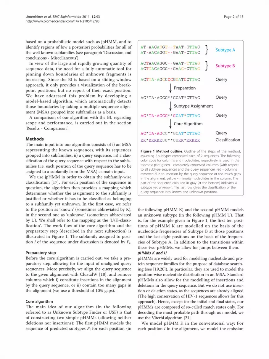
classification [17]. For each position of the sequence inquestion, the algorithm then provides a mapping whichdetermines whether the assignment to the subfamily isjustified or whether it has to be classified as belongingto a subfamily yet unknown. In the first case, we referto the position as ‘known’ (sometimes abbreviated by K),in the second one as ‘unknown’ (sometimes abbreviatedby U). We shall refer to the mapping as the ‘U/K-classi-fication’. The work flow of the core algorithm and thepreparatory step (described in the next subsection) isillustrated in Figure 1. The subfamily assigned to posi-tion i of the sequence under discussion is denoted by Fi.

Preparatory stepBefore the core algorithm is carried out, we take a pre-paratory step, allowing for the input of unaligned querysequences. More precisely, we align the query sequenceto the given alignment with ClustalW [18], and removecolumns which i) constitute insertions in the alignmentby the query sequence, or ii) contain too many gaps inthe alignment (we use a threshold of 10% gaps).

Core algorithmThe main idea of our algorithm (in the followingreferred to as Unknown Subtype Finder or USF) is thatof constructing two simple pHMMs (allowing neitherdeletions nor insertions): The first pHMM models thesequence of predicted subtypes Fi for each position (in

the following pHMM K) and the second pHMM modelsan unknown subtype (in the following pHMM U). Thatis, for the example given in Figure 1, the first ten posi-tions of pHMM K are modelled on the basis of thenucleotide frequencies of Subtype B at those positionsand the last eight positions on the basis of the frequen-cies of Subtype A. In addition to the transitions withinthese two pHMMs, we allow for jumps between them.pHMMs K and UpHMMs are widely used for modelling nucleotide and pro-tein sequence families for the purpose of database search-ing (see [19,20]). In particular, they are used to model theposition-wise nucleotide distribution in an MSA. StandardpHMMs also allow for the modelling of insertions anddeletions in the query sequence. But we do not use inser-tion or deletion states, as the sequences are already aligned(The high conservation of HIV-1 sequences allows for thisapproach). Hence, except for the initial and final states, ourpHMMs are composed of so-called match states only. Fordecoding the most probable path through our model, weuse the Viterbi algorithm [21].We model pHMM K in the conventional way: For

each position i in the alignment, we model the emission

AT-AACACGT--TAAT-CTTACAT-AACAGGT--GAAT-CTTAC

ACTAACAGGC--GAAT-TTTAGACTTACAGGC--GAAC-CTTAG

ACTTA-AGCCCCGCATCCTTAC

AC*TA-AGCC**GCAT*CTTAC

}}

Subtype A

Subtype B

Query

Query

Preparation

AC*TA-AGCC**GCAT*CTTAC Query

Subtype Assignment

AC*TA-AGCC**GCAT*CTTAC

KK*KKKKKUU**UUKK*KKKKK

Query

Classification

Core Algorithm

Figure 1 Method outline. Outline of the steps of the method,assuming 2 subtypes composed each of 2 sequences. The followingcolor code for columns and nucleotides, respectively, is used in thetopmost part: green - completely conserved columns (with respectto all subtype sequences and the query sequence), red - columnsremoved due to insertion by the query sequence or too much gapsin the alignment, yellow - minority nucleotides in the column. Thepart of the sequence coloured in gray (at the bottom) indicates asubtype yet unknown. The last row gives the classification of thequery sequence into known and unknown positions.


Page 2 of 13

probabilities �p of the i-th state of the pHMM K on thebasis of the nucleotide frequencies of Fi. To this end,choosing a Bayesian approach to model the emissionfrequencies, we assume that the a priori distribution of�p is a Dirichlet distribution (see [22]), with parameter �α(estimated in [17]). The parameter may be interpretedas pseudo counts which are added to the nucleotidefrequencies. The emission probabilities then are thecorresponding relative frequencies of these modifiednucleotide frequencies.For pHMM U, we have to choose another approach,

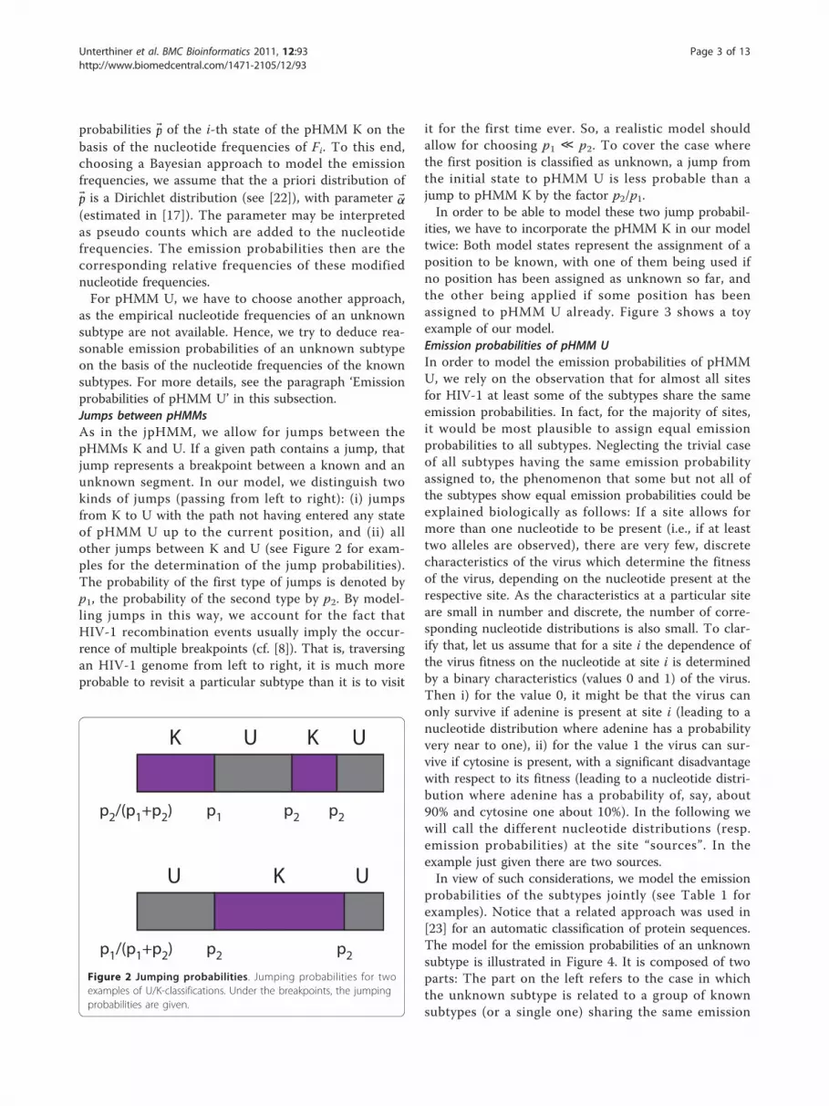
as the empirical nucleotide frequencies of an unknownsubtype are not available. Hence, we try to deduce rea-sonable emission probabilities of an unknown subtypeon the basis of the nucleotide frequencies of the knownsubtypes. For more details, see the paragraph ‘Emissionprobabilities of pHMM U’ in this subsection.Jumps between pHMMsAs in the jpHMM, we allow for jumps between thepHMMs K and U. If a given path contains a jump, thatjump represents a breakpoint between a known and anunknown segment. In our model, we distinguish twokinds of jumps (passing from left to right): (i) jumpsfrom K to U with the path not having entered any stateof pHMM U up to the current position, and (ii) allother jumps between K and U (see Figure 2 for exam-ples for the determination of the jump probabilities).The probability of the first type of jumps is denoted byp1, the probability of the second type by p2. By model-ling jumps in this way, we account for the fact thatHIV-1 recombination events usually imply the occur-rence of multiple breakpoints (cf. [8]). That is, traversingan HIV-1 genome from left to right, it is much moreprobable to revisit a particular subtype than it is to visit

it for the first time ever. So, a realistic model shouldallow for choosing p1 ≪ p2. To cover the case wherethe first position is classified as unknown, a jump fromthe initial state to pHMM U is less probable than ajump to pHMM K by the factor p2/p1.In order to be able to model these two jump probabil-

ities, we have to incorporate the pHMM K in our modeltwice: Both model states represent the assignment of aposition to be known, with one of them being used ifno position has been assigned as unknown so far, andthe other being applied if some position has beenassigned to pHMM U already. Figure 3 shows a toyexample of our model.Emission probabilities of pHMM UIn order to model the emission probabilities of pHMMU, we rely on the observation that for almost all sitesfor HIV-1 at least some of the subtypes share the sameemission probabilities. In fact, for the majority of sites,it would be most plausible to assign equal emissionprobabilities to all subtypes. Neglecting the trivial caseof all subtypes having the same emission probabilityassigned to, the phenomenon that some but not all ofthe subtypes show equal emission probabilities could beexplained biologically as follows: If a site allows formore than one nucleotide to be present (i.e., if at leasttwo alleles are observed), there are very few, discretecharacteristics of the virus which determine the fitnessof the virus, depending on the nucleotide present at therespective site. As the characteristics at a particular siteare small in number and discrete, the number of corre-sponding nucleotide distributions is also small. To clar-ify that, let us assume that for a site i the dependence ofthe virus fitness on the nucleotide at site i is determinedby a binary characteristics (values 0 and 1) of the virus.Then i) for the value 0, it might be that the virus canonly survive if adenine is present at site i (leading to anucleotide distribution where adenine has a probabilityvery near to one), ii) for the value 1 the virus can sur-vive if cytosine is present, with a significant disadvantagewith respect to its fitness (leading to a nucleotide distri-bution where adenine has a probability of, say, about90% and cytosine one about 10%). In the following wewill call the different nucleotide distributions (resp.emission probabilities) at the site “sources”. In theexample just given there are two sources.In view of such considerations, we model the emission

probabilities of the subtypes jointly (see Table 1 forexamples). Notice that a related approach was used in[23] for an automatic classification of protein sequences.The model for the emission probabilities of an unknownsubtype is illustrated in Figure 4. It is composed of twoparts: The part on the left refers to the case in whichthe unknown subtype is related to a group of knownsubtypes (or a single one) sharing the same emission

p1/(p

1+p

2) p

2p

2

U UK

p2/(p

1+p

2) p

1p

2p

2

U UKK

Figure 2 Jumping probabilities. Jumping probabilities for twoexamples of U/K-classifications. Under the breakpoints, the jumpingprobabilities are given.


Page 3 of 13

probability at the respective site. The part on the rightconcerns the case of an unknown subtype with charac-teristics leading to emission probabilities (at the respec-tive sites) yet unobserved (among the known subtypes).To construct the left-hand part of the model, we use a

Bayesian approach to determine position-wise an opti-mal number of sources and how the subtypes should beassigned to the sources. For each source the emission

probabilities are estimated on the basis of the emissionfrequencies of the subtypes assigned to the source. Theprobability, with which a source is chosen, is propor-tional to the number of subtypes assigned to it. Theright-hand part is modelled by a Dirichlet distributionwith the same value for the parameter �α as in paragraph‘pHMMs K and U’ of this subsection. We denote the apriori probability of a source involved, but yet unknown,

MK1 MK2 MK3 MK4

A 0.01C 0.01

G 0.97T 0.01

A 0.09C 0.02

G 0.11T 0.78

A 0.01C 0.02

G 0.02T 0.95

A 0.96C 0.02

G 0.01T 0.01

B

MK2 MK3 MK4

A 0.09C 0.02

G 0.11T 0.78

A 0.01C 0.02

G 0.02T 0.95

A 0.96C 0.02

G 0.01T 0.01

MU1 MU2 MU3 MU4

A 0.05C 0.03

G 0.91T 0.01

A 0.04C 0.02

G 0.54T 0.40

A 0.09C 0.01

G 0.02T 0.88

A 0.71C 0.22

G 0.03T 0.04

E

Figure 3 Model. The model underlying USF, illustrated by a toy example. The example uses an alignment and a query sequence of length 4.The query sequence is composed of the nucleotide sequence GTAA. The top row and bottom row of states each constitute a pHMM K, themiddle one pHMM U. The top pHMM K models the situation of pHMM U not having been visited yet, the bottom one that of pHMM U havingbeen visited already. Above and below, respectively, the states, their emission probabilities are given, with the nucleotide in the query sequencebeing marked red for the states in the Viterbi path. To the very left, resp. the very right, the initial, resp. the final state are situated. The short-dashed arrows represent transitions with probability p2, the long-dashed ones transitions with probability p1. The dotted arrows constitutetransitions from and to special states (initial and final state). The Viterbi path is colored in red, with the first two positions and the last position ofthe query sequence being classified as ‘known’ and the third position as ‘unknown’. Notice that the first state of the bottom pHMM K is missingsince this pHMM can only be entered if pHMM U has been visited before.

Table 1 Examples of calculation of emission probabilities

Pos. Sub./Src. A B C D 1 2 3

Nucl. G T G T G T G T G T G T G T

1 freq 89 0 360 0 393 0 3 0 846 0

p 0.9989 0.0011 0.9997 0.0003 0.9997 0.0003 0.969 0.031 0.9999 0.0001

2 freq 65 24 355 5 382 11 3 0 65 24 740 19

p 0.73 0.27 0.986 0.014 0.972 0.028 0.969 0.031 0.73 0.27 0.975 0.025

3 freq 30 59 325 35 364 29 0 3 30 59 689 64 0 3

p 0.34 0.66 0.903 0.097 0.926 0.074 0.0031 0.969 0.34 0.66 0.915 0.085 0.0031 0.969

Simplified example of position- and subtype-wise nucleotide frequencies of HIV. For three sites the subtype-wise nucleotide frequencies for subtypes A, B, C, andD are given on the left side of the table. Below them the emission probabilities estimated on the basis of only on the frequencies of the respective subtypes(using �α = (0.1, 0.1)) are shown. The different typefaces (regular, bold, italic) indicate which subtypes should be jointly modelled (i.e. belong to the samesource). On the right-hand side of the table, the nucleotide frequencies of the sources (i.e. the aggregated frequencies of the subtypes belonging to it) and theemission probabilities estimated on the basis of these frequencies are given (using the same �α). For the sake of simplicity, only the nucleotides G and T areassumed to exist. Apart from this simplification and the restriction to 4 subtypes, the example is taken from actual HIV-1 sequences.


Page 4 of 13

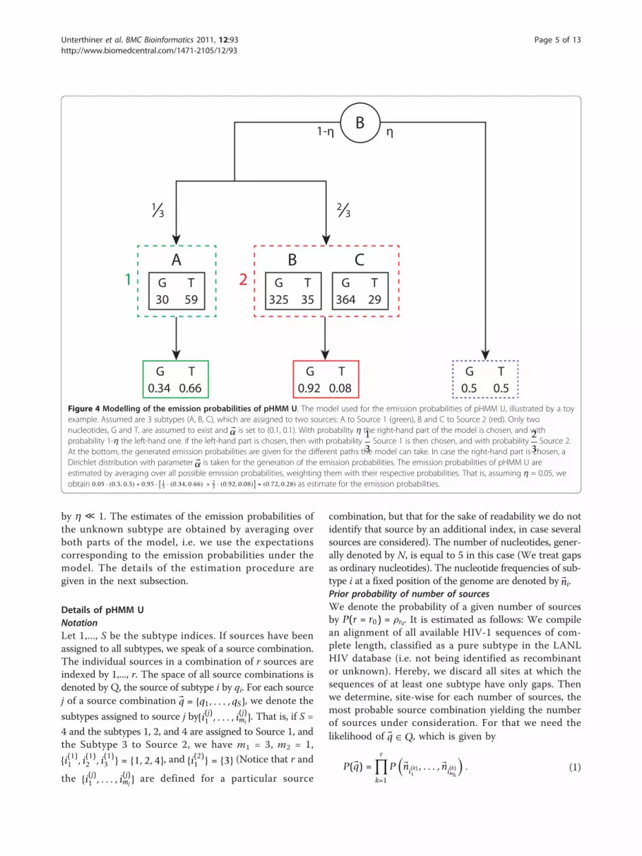
by h ≪ 1. The estimates of the emission probabilities ofthe unknown subtype are obtained by averaging overboth parts of the model, i.e. we use the expectationscorresponding to the emission probabilities under themodel. The details of the estimation procedure aregiven in the next subsection.

Details of pHMM UNotationLet 1,..., S be the subtype indices. If sources have beenassigned to all subtypes, we speak of a source combination.The individual sources in a combination of r sources areindexed by 1,..., r. The space of all source combinations isdenoted by Q, the source of subtype i by qi. For each sourcej of a source combination �q = {q1, . . . , qS}, we denote thesubtypes assigned to source j by{i(j)

1 , . . . , i(j)mj }. That is, if S =

4 and the subtypes 1, 2, and 4 are assigned to Source 1, andthe Subtype 3 to Source 2, we have m1 = 3, m2 = 1,

{i(1)1 , i(1)

2 , i(1)3 } = {1, 2, 4}, and {i(2)

1 } = {3} (Notice that r andthe {i(j)

1 , . . . , i(j)mj } are defined for a particular source

combination, but that for the sake of readability we do notidentify that source by an additional index, in case severalsources are considered). The number of nucleotides, gener-ally denoted by N, is equal to 5 in this case (We treat gapsas ordinary nucleotides). The nucleotide frequencies of sub-type i at a fixed position of the genome are denoted by �ni.Prior probability of number of sourcesWe denote the probability of a given number of sourcesby P(r = r0) = ρr0. It is estimated as follows: We compilean alignment of all available HIV-1 sequences of com-plete length, classified as a pure subtype in the LANLHIV database (i.e. not being identified as recombinantor unknown). Hereby, we discard all sites at which thesequences of at least one subtype have only gaps. Thenwe determine, site-wise for each number of sources, themost probable source combination yielding the numberof sources under consideration. For that we need thelikelihood of �q ∈ Q, which is given by

P(�q) =r∏

k=1

P(�ni(k)

1, . . . , �ni(k)

mk

). (1)

32

31

1-η ηB

21

0.5 0.5G T

0.92 0.08G T

0.34 0.66G T

30 59G T

A

364 29G T

C

325 35G T

B

Figure 4 Modelling of the emission probabilities of pHMM U. The model used for the emission probabilities of pHMM U, illustrated by a toyexample. Assumed are 3 subtypes (A, B, C), which are assigned to two sources: A to Source 1 (green), B and C to Source 2 (red). Only twonucleotides, G and T, are assumed to exist and �α is set to (0.1, 0.1). With probability h the right-hand part of the model is chosen, and withprobability 1-h the left-hand one. If the left-hand part is chosen, then with probability

13Source 1 is then chosen, and with probability

23Source 2.

At the bottom, the generated emission probabilities are given for the different paths the model can take. In case the right-hand part is chosen, aDirichlet distribution with parameter �α is taken for the generation of the emission probabilities. The emission probabilities of pHMM U areestimated by averaging over all possible emission probabilities, weighting them with their respective probabilities. That is, assuming h = 0.05, weobtain 0.05 · (0.5, 0.5) + 0.95 · [ 1

3 · (0.34, 0.66) + 23 · (0.92, 0.08)

]= (0.72, 0.28) as estimate for the emission probabilities.


Page 5 of 13

The probabilities on the right hand side of (1) canbe calculated as described in the following. Forthe next step we restrict ourselves to the case that

{i(k)1 , . . . , i(k)

mj } = {1 , . . . , m} for notational convenience

and make use of the equations

P(�n|�p) = �(|�n| + 1)N∏

j=1

pnj

j

�(nj + 1)(2)

and

P(�p) =� (|�α|)

�(∏N

j=1 αj

) N∏j=1

pαj−1j (3)

as well as

∫�p

N∏j=1

pβj−1j d�p =

∏Nj=1 �

(βj

)�

(| �β |

) , (4)

With b1,..., bN ≥ 0. Here, �α denotes the parameter of theDirichlet distribution introduced in the paragraph ‘Meth-ods - Core algorithm - pHMMs K and U’. Thus, we obtain

P(�n1, . . . , �nm)

=∫

�pP

(�n1, . . . , �nm|�p) P(�p) d�p

=∫

�p

(m∏

i=1

P(�ni|�p

))P

(�p) d�p

=∫

�p

⎡⎣ m∏

i=1

⎛⎝�

(| �ni | + 1) N∏

j=1

pni,j

j

�(ni,j + 1)

⎞⎠

⎤⎦ ×

⎡⎣ � (| �α |)

�(∏N

j=1 αj

) N∏j=1

pαj−1j

⎤⎦ d�p

=

(m∏

i=1

�(| �ni | + 1

)∏N

j=1 �(ni,j + 1

))

�(| �α |)�

(∏Nj=1 �αj

)×

∏Nj=1 �

(∑mi=1 ni,j + αj

)�

(∑mi=1 | �ni | + | �α |) .

Using (1) and the AIC (Akaike Information Criterion[24]), we deduce the most plausible source combinationfor each site and with that the most plausible number ofsources. Estimating the rj as the empirical frequencies ofthe number of sources (considering all eligible sites), weobtain the values (rj)j = 1,2,3 = (0.85, 0.09, 0.06). For thesake of computational efficiency, we restrict the number ofsources to values lower or equal to 3. Notice that thenumber of sources to which one can restrict the algorithmdepends on the scale of the intersubtype variation of thevirus genome at the informative sites of the genome.

Estimation of emission probabilitiesUsing

P(�q | �ρ) = ρr

r∏k=1

P(�ni(k)

1, . . . , �ni(k)

mk

),

we deduce the most likely source combination. Then,for a given source combination �q ∈ Q, we can estimatethe emission probability of a nucleotide v for a particu-lar source (assuming, for notational convenience, thatthe source under consideration is composed of the sub-types 1,..., m) by

p̂ν =∫�ppνP(�p |�n1, . . . , �nm)d�p. (5)

Using (2) and (3), we get

P(�p |�n1, . . . , �nm)

=P

(�n1, . . . , �nm|�p) P(�p)

P(�n1, . . . , �nm

)=

∏mi=1 P

(�ni|�p)

P(�p)

P(�ni, . . . , �nm

)=

⎡⎣ m∏

i=1

⎛⎝�

(|�ni| + 1) N∏

j=1

pni,j

j

�(ni,j + 1)

⎞⎠

⎤⎦×

� (| �α |)�

(∏Nj=1 αj

) N∏j=1

pαj−1j

/ [(m∏

i=1

�(| �ni| + 1

)∏N

j=1 �(ni,j + 1

))

×

� (| �α |)�

(∏Nj=1 αj

)∏N

j=1 �(∑m

i=1 ni,j + αi)

�(∑m

i=1 |�ni | + | �α |)⎤⎦

=�

(∑mi=1 |�ni | + | �α |)∏N

j=1 �(∑m

i=1 ni,j + αj) N∏

j=1

p∑m

i=1 ni,j+ αj−1j .

Consequently, we can transform (5) into

p̂ν =�

(∑mi=1 |�ni| + | �α |)∏N

j=1 �(∑m

i=1 ni,j + αi)×

∫�ppν

N∏j=1

p∑m

i=1 ni,j+ αj−1j d�p

Finally, by using (4) we obtain the simple formula

p̂ν =

∑mi=1 ni ,v + αν∑m

i=1 | �ni | + | �α | .


Page 6 of 13

ResultsIn this section, we present the results of i) the calibration ofUSF on a) artificial HIV-1 recombinants and b) non-recombinant HIV-1 sequences designated as havingemerged from a known subtype, ii) the application of USFto a) SIV sequences and b) sequences designated asunknown in the LANL HIV database (in the followingcalled “Subtype U” sequences), and iii) the comparison ofUSF and BI.

CalibrationIn order to calibrate USF and to investigate its behaviourin dependence of the choice of the parameters h, p1 andp2, we use two test settings, one of them suitable to assessthe sensitivity of the algorithm, the other one the specifi-city. For the sensitivity, we remove one subtype from theMSA and consider it as unknown. Then we generate artifi-cial recombinants of sequences from the “known” subtypesand the “unknown” subtype. For the specificity, we simplycheck whether sequences from the MSA are classified cor-rectly. In both cases, we do not use the test data as train-ing data for the emission probabilities of the HMMs. Thetesting setup is sketched in Figure 5. The MSA consists inall full-length HIV-1 Group M sequences, designated asstemming from a pure subtype in the LANL database,downloaded on 9th of July 2010.Test dataMore precisely, we generate the following two sets oftest sequences: (i) A set Tsens for measuring the

sensitivity with respect to the ability of the algorithm todetect genome segments stemming from an unknownsubtype, and (ii) a set Tspec for measuring the specificity.The set Tsens is composed of 229 sequences generatedby taking a sequence from subtypes A-D and F-G andreplacing a segment of this sequence by a segment of asequence from some other subtype. We call the subtypeof the major part of the genome the ‘base subtype’ andthe subtype of the inserted part of the genome the‘insertion subtype’. A preliminary analysis shows that incase the subtypes H, J, or K have been assigned to thequery sequence (or a part of it), USF is not suitable fora reliable detection of unclassifiable genome parts.Hence, for the role of a base subtype, those subtypes areexcluded from our analysis. Nevertheless, segments ofthem may play the role of insertion subtypes. Segmentsof the subtypes B and D may not be combined, due tothe small phylogenetic distance of those subtypes. More-over, the replaced segments have a length of 1000 posi-tions and their position has been chosen randomly. Tspec

is composed of 265 sequences sampled from the gen-ome-length sequences being classified as subtype A-Dor F-G in the LANL HIV database (50 for all subtypesexcept for the subtypes F and G, for which only 35 and30, respectively, sequences were available). For Tspec thesequences were assigned to the subtype they stem fromaccording to their LANL HIV database designation.Therefore, if classified correctly, the complete sequenceis classified as known. Any detected unknown regions

Tsens

A

A B C A

AG

jpHMM

USF

genome data

K KU

Tspec

A

A

USF

K

U/K classification

subtype classification

Figure 5 Test setup. Testing is performed on two sets of sequence data, Tsens and Tspec. For Tsens artificial recombinants of two subtypes areused as genome data, for Tspec pure sequences are taken. The sequences of Tsens are classified subtype-wise with jpHMM, whereas thesequences of Tspec are assigned their original subtype. Then, USF is applied to both sequence sets.


Page 7 of 13

are counted as false positives. For Tsens we determinethe subtype classification using the jpHMM, excludingthe subtypes H, J, and K from the assignable subtypes.Test resultsWe measure the performance by counting how manypositions in a sequence have been misclassified. Settingp1 = 10-7 and p2 = 10-4 (which seem to be reasonablevalues, in view of our experience gathered when apply-ing the jpHMM to HIV), we determine h = 0.05 as lead-ing to the best tradeoff between sensitivity andspecificity. With that choice of h, we evaluate the per-formance with respect to specificity and sensitivity on agrid for different choices of p1 and p2 (see Figure 6 and7). From those data, we would recommend to choosep1 = 10-9 and p2 = 10-5. In case a user has a different

priority with respect to specificity and sensitivity, he canadapt the values to his purpose. To achieve a highersensitivity or specificity, p1 and p2 have to be increasedor decreased, respectively. Increasing p1 merely resultsin a higher probability of finding any Subtype U frag-ments in the query sequence at all, whereas increasingp2 also leads to a higher number of Subtype U frag-ments to be found.In Figure 8, resp. 9, the performance of the algorithm

for Tspec, resp. Tsens is displayed stratified by the assignedsubtype Tsens, resp. the subtypes used for generating theartificial recombinants. Among the 6 sequences fromTspec, which yield the most misclassified positions, thereare all 4 sequences of Subsubtype F2 and the sequencefrom Subsubtype F1, which cluster most closely to

10−5

10−6

10−7

10−8

10−9

10−10

10−11

10−12

10−3

10−4

10−5

10−6

10−7

10−8

60

70

80

90

100

p1p2

mea

n pe

rfor

man

ce

Figure 6 Mean performance of Tspec. The mean performance (measured in misclassified positions) of Tspec in dependence of p1 and p2 (bothscaled logarithmically).


Page 8 of 13

Subsubtype F2 in a phylogenetic tree (using FastTree [25]and FigTree [26]).To facilitate the testing technically, we restrict our

analysis to the positions 808 to 8781 with respect toHXB [27]. Covering this part of the genome, we analysethe performance of USF in relatively conserved regions,as well as highly variable ones and we do not have tocope with the low number of sequences available forcovering the boundary parts of the genome.Theoretical determination of hWe have tried also to determine h by a theoreticalapproach. More precisely, we have simulated unknownsubtypes by excluding a subtype from the data based onwhich the emission probabilities of pHMM U were

estimated. We then have chosen h such that the emis-sion frequencies of the excluded subtype is estimatedbest (with respect to maximum likelihood). Unfortu-nately, this approach has filed to values of h smaller byan entire order of magnitude than the values found bymeans of the calibration described above. Consequently,we refrain from using this theoretical approach.

SIV sequences and Subtype U sequencesIn order to check whether USF correctly classifies verydivergent sequences, we have applied it to five full-length SIV genomes (AF103818, DQ373063, EF394356,U42720, X52154) from different parts of the SIV clade.As before, we did not allow for assigning subtypes H, J,

10−5

10−6

10−7

10−8

10−9

10−10

10−11

10−1210−3

10−4

10−5

10−6

10−7

10−8

380

400

420

440

460

p1

p2

mea

n pe

rfor

man

ce

Figure 7 Mean performance of Tsens. The mean performance (measured in misclassified positions) of Tsens in dependence of p1 and p2 (bothscaled logarithmically).


Page 9 of 13

and K in the subtype classification. In the same way wehave tested the 8 full-length Subtype U genomes(AF286236, AF457101, AY046058, EF029066, EF029067,EF029068, EF029069, FJ388921). Except the Subtype Usequence AY046058, all sequences have been correctlyidentified as completely unknown (about 8% of thegenome have not been classified as unknown).

Comparison with the BIThe BI is a method based on distance and phylogeny. Itdetermines which parts of a query sequence should beclassified among known sequences. Moving along thegenome of a query sequence with a sliding window, theBI computes a ratio quantifying how closely the querysequence clusters with a subtype clade. On the basis ofthis quantity, it determines whether the respective partof a query sequence is unclassifiable with respect to theknown subtypes.We apply the BI to a subset of Tspec, as well as the SIV

and Subtype U sequences used in the evaluationdescribed in the subsection ‘Results - SIV sequences andSubtype U sequences’. As we had to carry out the test-ing manually, using the web interface of the BI [28], wehad to confine ourselves to a limited number ofsequences from Tspec and could not test the BI on Tsens

at all. (For the purpose of the latter, it would have beennecessary to reestimate the parameters of the BI afterhaving removed a subtype from the training data. That,however, the web interface available does not allow.)Application of the BI to the 5 SIV sequences and the

8 Subtype U sequences from the subsection ‘Results -SIV sequences and Subtype U sequences’ yields validresults in 3 and 4 cases, respectively. Out of these 7sequences, all but one Subtype U sequence (AY046058)are classified correctly as completely unknown, withabout 6% of the genome of AY046058 beingmisclassified.Testing the BI on 12 sequences for each subtype from

Tspec, yield the results illustrated in Figure 10. Since USFtends to misclassify very short segments as unknown forsome subtypes, we also compare the BI with USF,removing all segments of length smaller than 100 bpsfrom the outcome of USF.Using the two-sided Wilcoxon signed-rank test, the

version of USF without postprocessing performs signifi-cantly better (with respect to our position-wise measure)than the BI for the subtypes A and B. For the Subtype F,the BI is significantly better than USF (p = 0.05). For theother subtypes, this test does not yield significantresults. If USF is used in the version equipped withpostprocessing, it yields significantly better results thanthe BI for the subtypes A and B, with the differences onthe other subtypes being highly insignificant.

A B C D F G

Subtype

Mea

n di

stan

ce

050

100

150

200

Figure 8 Mean subtype-wise performance of Tspec. The meanperformance (measured in misclassified positions) of Tspec for p1 =10-9 and p2 = 10-5, stratified by the assigned subtype.

A B C D F G H J K

Subtype of middle segment

G

F

D

C

B

A

Subt

ype

of fi

rst a

nd la

st s

egm

ent

200 400 600 800Mean performance

Color Key

Figure 9 Mean subtype-wise performance of Tsens. Level plot ofthe mean performance (measured in misclassified positions) of Tsensfor p1 = 10-9 and p2 = 10-5, stratified by the used subtypes. Differentcolors represent different levels of misclassification. White rectanglesrepresent subtype pairs which were not used in the generation ofTsens.


Page 10 of 13

Running timeExcluding the running time of ClustalW and jpHMM(described in [18,17]), the running time for a full lengthHIV-1 sequence is about 35 seconds on a Linux PCwith 3 GHz and 4 GB RAM.

Discussion and conclusionsWe have presented USF, a tool for detection of unclassi-fiable segments in viral sequences. Using a probabilistic,model-driven approach, the tool is suitable in principlefor all species (or other taxa) which are subdivided intosubfamilies i) without too many indels separating thesubfamilies and ii) where the phylogenetic distancesbetween the subfamilies are not too inhomogeneous.

TestingWe have applied USF to i) artificial recombinants of twosubtypes (excluding one subtype from the training datato simulate an unknown subtype), ii) sequences desig-nated (in the LANL HIV database) as originating from apure subtype, iii) SIV sequences, and iv) Subtype Usequences. As far as feasible, we have compared ourresults with the only other tool available with the samescope, the Branching Index (BI).

Performance of USFAnalyzing the performance of USF by subtype, one cansee that it performs considerably better (with respect to

specificity) on the subtypes A-C than on D, F, and G,whereas it does not yield acceptable results for the sub-types H, J, and K. Its unsatisfactory performance on thelast three subtypes does not come unexpectedly: Thesubtypes H, J, and K are composed of only 2 or 3 com-plete genome sequences, and that does not allow for arealistic modelling of the emission probabilities of apHMM without using an information sharing protocol(see [23]). The weaker performance for subtypes D, F,and G might also be explicable by this effect, with thesituation being obfuscated for the Subtype F by the factthat this subtype is divided into two subsubtypes.The results of the application of USF to artificial

recombinants can be explained in part also by the size ofthe involved subtypes: The poorest results are achievedwhen subtypes G or J, which both belong to the subtypesof smaller size, act as base subtype. Obviously, the size ofthe insertion subtype should not have any impact on theperformance of USF (and the results also do not suggestthat). Astonishingly, there does not seem to be a correla-tion between the phylogenetic distance of a pair of baseand insertion subtypes and the performance of USF onthe respective pair: Testing Tsens involves 46 pairs of sub-types. Considering the 13 pairs with the lowest phyloge-netic distance, none of them is among the 3 poorestperforming pairs and 3 are among the 7 poorest perform-ing. As we have observed a poor performance of USFwhen the subtypes B and D are the base and insertionsubtypes, we may conclude that, if the phylogenetic dis-tance of the subtype pair is above a certain threshold, theperformance of USF does not seem to depend on howremotely the subtypes are related exactly.

Specificity of USF & BIComparing USF (employing the removal of very shortsegments in the outcome) with the BI with respect tospecificity, USF, roughly speaking, performs better onsome of the large size subtypes (A and B), whereas thereare no significant differences on the large size Subtype Cand the smaller size subtypes D, F, and G.

Sensitivity of USF & BIFor a comparison of the sensitivities we had to restrictourselves to the SIV and Subtype U sequences. In spiteof the importance of the sensitivity to assess the perfor-mance of USF and BI, the analysis of this characteristichad to be carried out on quite a small test set, due totechnical limitations in the implementation of the BI.Except for the Subtype U sequence AY046058, all SIVand Subtype U sequences were classified as unknown byUSF as well as the BI. Since both tools detect the samesequence as not completely unknown (although differentsegments were detected as known), this might be a hintthat the classification of AY046058 as a pure Subtype U

A B C D F G

Subtype

Mea

n di

stan

ce

0.0

0.2

0.4

0.6

0.8

1.0

BIUSF w/o postprocessingUSF

Figure 10 Comparison of USF and BI. The mean performance(measured in terms of the fraction of misclassified positions) for 12random sequences of each subtype for the BI and USF, stratified by theassigned subtype. For USF the results with all segments of length lessthan 100 bps (green) and without such a removal (green) are displayed.


Page 11 of 13

sequence is questionable. To conclude, our analysis doesnot reveal any significant differences between USF andthe BI with respect to their sensitivity.

Versatility of USF & BIWith respect to versatility, the BI seems to be slightlyinferior to USF (at least in their current versions). As itis not possible to determine h by a theoretical approach(as described in paragraph ‘Results - Calibration - Theo-retical determination of h’), both methods require aparameter calibration on training data when applied to anew species, respectively taxon. Regarding breakpointpositions, the BI only provides a graph from which theuser would have to deduce the breakpoint positions byvisual inspection. Hence, it is not possible to run anyautomated procedures on the BI if breakpoint positionsare required.

OutlookIn the near future, we plan to incorporate our methodin the jpHMM. This would lead to a tool capable notonly of assigning the known subtypes of HIV-1 (or sub-families of other viruses or species) to a query sequence(or parts of it) but also of detecting segments of thegenome stemming from a subtype yet unknown. More-over, we are currently working on the implementationof an information sharing protocol for the jpHMM,which then would attenuate the poor performance ofUSF when applied to the small size subtypes.In addition, it has been discussed whether the core

gene of some D/E-recombinants of Hepatitis B virus(HBV) might stem from a clade which became rare orextinct [29]. We will apply USF to HBV data in order toinvestigate this question.Furthermore, it has been claimed that the HBV geno-

type G is a recombinant between i) an ancestor compar-able in divergence to those between the genotypes A-E,contributing the S gene, and ii) an HBV variant which ismuch more divergent, contributing the rest of the gen-ome [30]. In the face of this finding, we plan to incorpo-rate more than one unknown subtype in our model sothat different degrees of divergence can be modelled.

MiscellaneousAs mentioned in the section ‘Background’, it is not pos-sible to find unknown sequence segments by identifyingregions of small a posterior probabilities for all of theknown subfamilies when applying the jpHMM forexample. That is easily exemplified as follows: Let usassume there were only two subtypes A and B and weexamined a sequence stemming from an unknown sub-type which is genetically considerably closer to SubtypeA than to Subtype B. Then this sequence would achievevery large a posteriori probabilities for Subtype A and

very small ones for Subtype B. Thus, it would falsely beclassified as known.USF is implemented in C++ and the source code is

freely available (see additional file 1).

Additional material

Additional file 1: Source code. C++ implementation of USF.

AcknowledgementsWe would like to thank Thomas Leitner for the encouragement to developUSF and Heinrich Hering for proofreading. This work was supported by theDeutsche Forschungsgemeinschaft (STA 1009/5-1).

Author details1Institute of Microbiology and Genetics, University of Göttingen,Goldschmidtstr. 1, 37077 Göttingen, Germany. 2LMNO, Université de Caen,CNRS UMR 6139, 14032 Caen Cedex, France. 3Institut für Mathematik undInformatik, Walther-Rathenau-Straße 47, 17487 Greifswald, Germany.

Authors’ contributionsTU implemented and validated the algorithm. AKS carried out modificationson jpHMM. JB provided statistical expertise. MS and BM guided the project,MS contributed to the model development. IB conceived the approach,developed, implemented and tested the algorithm and supervised theprogram development. All authors read and approved the final manuscript.

Received: 28 September 2010 Accepted: 11 April 2011Published: 11 April 2011

References1. Korber B, Gaschen B, Yusim K, Thakallapally R, Kesmir C, Detours V:

Evolutionary and immunological implications of contemporary HIV-1variation. Br Med Bull 2001, 58:19-42.

2. Leitner T: The molecular epidemiology of human viruses Springer Berlin;2002.

3. Hraber P, Fischer W, Bruno W, Leitner T, Kuiken C: Comparative analysis ofhepatitis C virus phylogenies from coding and non-coding regions: the5’ untranslated region (UTR) fails to classify subtypes. Virology Journal2006, 3:103.

4. Rhodes T, Wargo H, Hu WS: High Rates of Human ImmunodeficiencyVirus Type 1 Recombination: Near-Random Segregation of Markers OneKilobase Apart in One Round of Viral Replication. J Virol 2003,77(20):11193-11200.

5. Hahn BH, Shaw GM, De KM, Sharp PM: AIDS as a Zoonosis: Scientific andPublic Health Implications. Science 2000, 287(5453):607-614.

6. Robertson DL, Anderson JP, Bradac JA, Carr JK, Foley B, Funkhouser RK,Gao F, Hahn BH, Kalish ML, Kuiken C, Learn GH, Leitner T, McCutchan F,Osmanov S, Peeters M, Pieniazek D, Salminen M, Sharp PM, Wolinsky S,Korber B: HIV-1 nomenclature proposal. Science 2000, 288:55-57.

7. Hoelscher M, Dowling WE, Sanders-Buell E, Carr JK, Harris ME, Thomschke A,Robb ML, Birx DL, McCutchan FE: Detection of HIV-1 subtypes,recombinants, and dual infections in East Africa by a multi-regionhybridization assay. AIDS 2002, 16:2055-2064.

8. LANL HIV Databases: CRFs. 2011 [Http://www.hiv.lanl.gov/content/sequence/HIV/CRFs/CRFs.html].

9. de Oliveira T, Deforche K, Cassol S, Salminen M, Paraskevis D, Seebregts C,Snoeck J, van Rensburg EJ, Wensing AMJ, van de Vijver DA, Boucher CA,Camacho R, Vandamme AM: An automated genotyping system foranalysis of HIV-1 and other microbial sequences. Bioinformatics 2005,21(19):3797-3800.

10. Recombinant Identification Program Web Interface. [http://www.hiv.lanl.gov/content/sequence/RIP/RIP.html].

11. Zhang M, Schultz AK, Calef C, Kuiken C, Leitner T, Korber B, Morgenstern B,Stanke M: jpHMM at GOBICS: a web server to detect genomicrecombinations in HIV-1. Nucleic Acids Res 2006, 34(S2):W463-465.


Page 12 of 13

http://www.biomedcentral.com/content/supplementary/1471-2105-12-93-S1.ZIP

http://www.ncbi.nlm.nih.gov/pubmed/11714622?dopt=Abstract














Http://www.hiv.lanl.gov/content/sequence/HIV/CRFs/CRFs.html

Http://www.hiv.lanl.gov/content/sequence/HIV/CRFs/CRFs.html



http://www.hiv.lanl.gov/content/sequence/RIP/RIP.html

http://www.hiv.lanl.gov/content/sequence/RIP/RIP.html



12. Schultz AK, Zhang M, Bulla I, Leitner T, Korber B, Morgenstern B, Stanke M:jpHMM: Improving the reliability of recombination prediction in HIV-1.Nucl Acids Res 2009, , 37 Web Server: W647-651.

13. Maydt J, Lengauer T: Recco: recombination analysis using costoptimization. Bioinformatics 2006, 22(9):1064-1071.

14. Pandit A, Sinha S: Using genomic signatures for HIV-1 sub-typing. BMCBioinformatics 2010, 11(Suppl 1):S26.

15. Wilbe K, Salminen M, Laukkanen T, McCutchan F, Ray SC, Albert J, Leitner T:Characterization of novel recombinant HIV-1 genomes using thebranching index. Virology 2003, 316:116-125.

16. Hraber P, Kuiken C, Waugh M, Geer S, Bruno WJ, Leitner T: Classification ofhepatitis C virus and human immunodeficiency virus-1 sequences withthe branching index. J Gen Virol 2008, 89(9):2098-2107.

17. Schultz AK, Zhang M, Leitner T, Kuiken C, Korber B, Morgenstern B,Stanke M: A jumping profile Hidden Markov Model and applications torecombination sites in HIV and HCV genomes. BMC Bioinformatics 2006,7:265.

18. Chenna R, Sugawara H, Koike T, Lopez R, Gibson TJ, Higgins DG,Thompson JD: Multiple sequence alignment with the Clustal series ofprograms. Nucl Acids Res 2003, 31(13):3497-3500.

19. Krogh A, Brown M, Mian IS, Sjölander K, Haussler D: Hidden MarkovModels in Computational Biology: Applications to Protein Modeling.Journal of Molecular Biology 1994, 235(5):1501-1531.

20. Eddy S: Profile hidden Markov models. Bioinformatics 1998, 14(9):755-763.21. Viterbi A: Error bounds for convolutional codes and an asymptotically

optimum decoding algorithm. Information Theory, IEEE Transactions 1967,13(2):260-269.

22. Sjölander K, Karplus K, Brown M, Hughey R, Krogh A, Mian I, Haussler D:Dirichlet mixtures: a method for improved detection of weak butsignificant protein sequence homology. Comput Appl Biosci 1996,12(4):327-345.

23. Brown DP, Krishnamurthy N, Sjölander K: Automated Protein SubfamilyIdentification and Classification. PLoS Comput Biol 2007, 3(8):e160.

24. Akaike H: A new look at the statistical model identification. AutomaticControl, IEEE Transactions 1974, 19(6):716-723.

25. Price MN, Dehal PS, Arkin AP: FastTree: Computing Large MinimumEvolution Trees with Profiles instead of a Distance Matrix. Mol Biol Evol2009, 26(7):1641-1650.

26. FigTree. [Http://tree.bio.ed.ac.uk/software/gtree/].27. Korber B, Foley B, Kuiken C, Pillai S, Sodroski J: Numbering Positions in HIV

Relative to HXB2CG. Human Retroviruses and AIDS 1998, Los Alamos, NM:Theoretical Biology and Biophysics Group, Los Alamos National Laboratory1998, 102-111.

28. Branching Index Web Interface. [http://www.hiv.lanl.gov/content/sequence/phyloplace/PhyloPlace.html].

29. Simmonds P, Midgley S: Recombination in the Genesis and Evolution ofHepatitis B Virus Genotypes. J Virol 2005, 79(24):15467-15476.

30. Kato H, Orito E, Gish RG, Sugauchi F, Suzuki S, Ueda R, Miyakawa Y,Mizokami M: Characteristics of Hepatitis B Virus Isolates of Genotype Gand Their Phylogenetic Differences from the Other Six Genotypes (Athrough F). J Virol 2002, 76(12):6131-6137.

doi:10.1186/1471-2105-12-93Cite this article as: Unterthiner et al.: Detection of viral sequencefragments of HIV-1 subfamilies yet unknown. BMC Bioinformatics 201112:93.

Submit your next manuscript to BioMed Centraland take full advantage of:

• Convenient online submission

• Thorough peer review

• No space constraints or color figure charges

• Immediate publication on acceptance

• Inclusion in PubMed, CAS, Scopus and Google Scholar

• Research which is freely available for redistribution

Submit your manuscript at www.biomedcentral.com/submit


Page 13 of 13























Http://tree.bio.ed.ac.uk/software/gtree/

http://www.hiv.lanl.gov/content/sequence/phyloplace/PhyloPlace.html

http://www.hiv.lanl.gov/content/sequence/phyloplace/PhyloPlace.html






Documents

Detection of viral sequence fragments of HIV-1 subfamilies yet unknown