CZECH TECHNICAL UNIVERSITY IN PRAGUE Faculty of Electrical Engineering

Department of Electrical Power Engineering

Determination of Induction Motor Speed using

Kalman Filter

by

RANJAN TIWARI

Supervisor

Ing. PAVEL KARLOVSKY

A master thesis submitted to

The Faculty of Electrical Engineering, Czech Technical University in

Prague

Master Degree study program: Electrical Power Engineering

Prague, June 2019

_______________________________________________________________________

ii

_______________________________________________________________________

iii

Declaration

I, Ranjan Tiwari declare that the submitted work I have produced independently and have

listed all used information sources in accordance with the Methodological Guideline on

Ethical Principles of the Preparation of University Graduate Thesis.

Date:

Signature:

_______________________________________________________________________

iv

Abstract

This thesis describes the design and implementation of the discretized Extended

Kalman Filter (EKF) for the estimation of the speed of the induction motor. In this

implementation, the speed is treated as an additional state of the system and the EKF is

designed to estimate this state. The inputs for the filter are the inverter voltage and stator

currents. The simulations are carried out in Matlab Simulink and after the verification of

the filter, the algorithm is tested with laboratory motor. The filter is implemented on the

dSPACE DS1103 microprocessor controlling unit, which also handles the real-time data

logging and visualization, and the control user interface. Predictive Torque Control (PTC)

strategy is employed for the motor drive. The experimental part presents the speed

determination accuracy in various working points including high and low speed areas.

Then the optimization of the filtering process for better response in transients and stable

states are performed. Finally, the results are evaluated.

Keywords: Induction Motor, Extended Kalman Filter, MATLAB/Simulink, dSPACE,

Sensorless Speed Determination

_______________________________________________________________________

v

Abstrakt

Tato práce popisuje návrh a implementaci diskretizovaného rozšířeného

Kalmanova filtru (EKF) pro odhad rychlosti asynchroního motoru. V této implementaci

EKF je rychlost motoru považována za další stav systému a filtr je navržen tak, aby

odhadoval právě tento stav. Vstupem pro filtr jsou napětí na výstupu měniče a statorové

proudy. Simulace jsou provedeny v prostředí Matlab Simulink a po ověření funkčnosti je

algoritmus otestován i na laboratorním motoru. Filtr je realizován na mikroprocesorové

řídicí jednotce dSPACE DS1103, která také obsluhuje záznam a vizualizaci dat v reálném

čase a uživatelské rozhraní ovládání. Pro řízení pohonu je použita strategie prediktivního

řízení momentu (PTC). V experimentální části je předvedena přesnost stanovení rychlosti

v různých pracovních bodech včetně oblastí vysokých a nízkých otáček. Dále je provedena

optimalizace filtru pro lepší odezvu v přechodových dějích i ve stabilních stavech.

Nakonec je proveden rozbor získaných výsledků.

Klíčová slova: Asynchronní motor, Rozšířený Kalmanův filtr, MATLAB/Simulink,

dSPACE, bezsenzorové zjišťování otáček

_______________________________________________________________________

vi

Acknowledgement

Throughout the writing of this thesis, I have received a great deal of support and assistance.

I would first like to thank my supervisor, Ing. Pavel Karlovsky, whose expertise was

invaluable in the formulation of the project topic and methodology in particular. He was

there to guide me at every step needed.

I would like to thank Prof. Ing. Jiří Lettl, CSc, for his assistance and guiding me

towards the topic for this thesis in the initial phase. I would like to acknowledge

my colleague from my class, Emre Sakar for his wonderful assistance during different

phases of writing this thesis.

I would also like to thank the Department of Electric Drives and Traction, CTU and the

faculty from there for assisting me in the laboratory issues during the experimentation

phase, and letting me conduct the experimental research in the laboratory.

In addition, I would like to thank my parents for their wise counsel and sympathetic ear.

Finally, there are my friends, Anup, Bishal, Dipesh, Sarjan, Madhu, Nishant, Biswash and

Aastha who were there to support me and providing happy distraction to rest of my mind

outside my research.

_______________________________________________________________________

vii

Dedication

To My Family and Friends

_______________________________________________________________________

viii

Contents

LIST OF FIGURES xi

ABBREVIATIONS xiii

1 INTRODUCTION 1

2 KALMAN FILTER AND ITS DESIGN FOR INDUCTION

MOTOR SPEED DETERMINATION

3

2.1 Kalman Filter 3

2.1.1 The Process to be Estimated 4

2.1.2 The Estimation Process 4

2.1.3 Mathematical Representation 5

2.2 Extended Kalman Filter 5

2.2.1 Mathematical Representation 6

2.3 Mathematical Model of the Induction Motor 6

2.4 Designing and Implementing the EKF to the Motor

Model

7

2.4.1 Extension of the State Vector to Add Rotor

Angular Speed as a State Variable

8

2.4.2 Discretization of the IM model 9

2.4.3 Determination of the Noise and State

Covariance Matrices

10

2.4.4 Implementation of EKF Algorithm 10

2.4.4.1 Initialization of State Vectors

and Covariance Matrices

11

2.4.4.2 Prediction of state variables 11

2.4.4.3 Estimation of Covariance Matric

of Prediction

12

2.4.4.4 Kalman Gain Computation 12

2.4.4.5 State Vector Estimation 13

2.4.4.6 Correction of the Covariance

Matrix of Prediction for next

loop

13

_______________________________________________________________________

ix

3 SIMULATION OF IM AND EKF IN SIMULINK MATLAB 14

3.1 Model of IM and Control Strategy 14

3.1.1 Reference Values Block 15

3.1.2 Predictive Control Block 15

3.1.3 Inverter Block 16

3.1.4 IM Model Block 17

3.2 EKF Model 18

3.2.1 EKF Algorithm 18

3.2.2 Tuning of the Noise Covariance Matrices Q

and R

20

3.3 Simulation Results from Matlab Simulink 21

3.4 Concluding the Simulation Results 27

4 DESCRIPTION OF THE WORKPLACE AND HARDWARE

ASSEMBLED

28

4.1 The Circuit Diagram 28

4.2 List of Hardware Assembled 28

5 EXPERIMENTAL RESULTS 33

5.1 Steady State Operation of Motor

5.1.1 Loaded Steady State Operation of the Motor 33

5.1.2 Unloaded steady state Operation of the Motor 34

5.1.3 Comparison of Loaded and Unloaded

Operation Mode

36

5.2 Tuning of Covariance Noise Matrices Q and R 36

5.2.1 Keeping R constant and varying Q in steady

state

37

5.2.2 Keeping Q constant and varying R 37

5.2.3 Varying Q while keeping R constant at 2000

in transients

38

5.3 Operations in Speed Reversal Mode with changing slew

rates

40

5.4 Low Speed Performance 42

5.5 Performance under varying load 42

_______________________________________________________________________

x

6 CONCLUSION 44

Work for Future 45

7 REFERENCES 47

APPENDIX 48

A.1 Parameters of IM 48

A.2 Equations of IM 48

_______________________________________________________________________

xi

List of Figures

2.1 Typical application of Kalman Filter 3

2.2 Structure of EKF 11

3.1 Simulink Model of the estimation of rotor speed of IM with

control mechanism 14

3.2 Reference Values Block 15

3.3 Block diagram schematic of IM drive Model Predictive

Control 16

3.4 Voltage vector diagram 17

3.5 IM block representation 17

3.6 EKF block 18

3.7 Simulation Results of IM parameters 22

3.8 Comparison of IM measured Current and EKF estimated Current

22

3.9 Comparison of IM measured Rotor Flux and EKF estimated

Rotor Flux 23

3.10 Simulation comparison between Measured IM speed and EKF estimated speed for 20 μs sampling time with noise

23

3.11 Detailed view of the speed comparison in steady state for

Figure 3.10 24

3.12 Simulation result comparison between Measured IM speed and EKF estimated speed for 150μs sampling time with

noise

24

3.13 Detailed view of the speed comparison in steady state for Figure 3.12

25

3.14 Simulation results without any noise and added offsets in

the Measured and estimated speeds 25

3.15 Detailed view of the speed comparison in steady state for

Figure 3.14 26

3.16 Simulation result comparison between Measured IM speed

and EKF estimated speed for 20μs sampling time and

observing the state of speed reversal with noise.

26

3.17 Detailed view of Figure 3.18 in the speed reversal region 27

4.1 Circuit schematic of the assembled circuit 28

4.2 Workplace and the assembled hardware 31

4.3 dSPACE control desk project UI 32

5.1 Loaded steady state operation of the motor 33

5.2 Detailed view of Figure 5.1 in the high-speed steady state

region

34

_______________________________________________________________________

xii

5.3 Unloaded steady state operation of the motor. 35

5.4 Detailed view of Figure 5.3 in the high-speed steady state

region

35

5.5 Comparison of loaded and unloaded operations mode in

steady state

36

5.6 Varying Matrix Q while keeping R constant at 2000 in

steady state

37

5.7 Varying Matrix R while keeping Q constant at 10 38

5.8 Varying Matrix Q while keeping R constant at 2000, for

transient response

38

5.9 Comparison of rise time during transients for different Q

values (R = 2000)

39

5.10 Comparison of fall time during transients for different Q

values (R = 2000)

39

5.11 Unloaded Speed Reversal Transients with slew rate of 1.5 40

5.12 Comparison of loaded Speed Reversal Transients with slew

rate of 0.05 and 1.5

41

5.13 Low-Speed performance with zero crossings (60 to -60 42

5.14 Measured and Estimated speed under varying loads with

various speed references

43

_______________________________________________________________________

xiii

Abbreviations

List of Abbreviations used in this thesis.

PE Power Electronics

VFD Variable Frequency Drives

IM Induction Motor

KF Kalman Filter

EKF Extended Kalman Filter

PTC Predictive Torque Control

_______________________________________________________________________

1

Chapter 1

Introduction

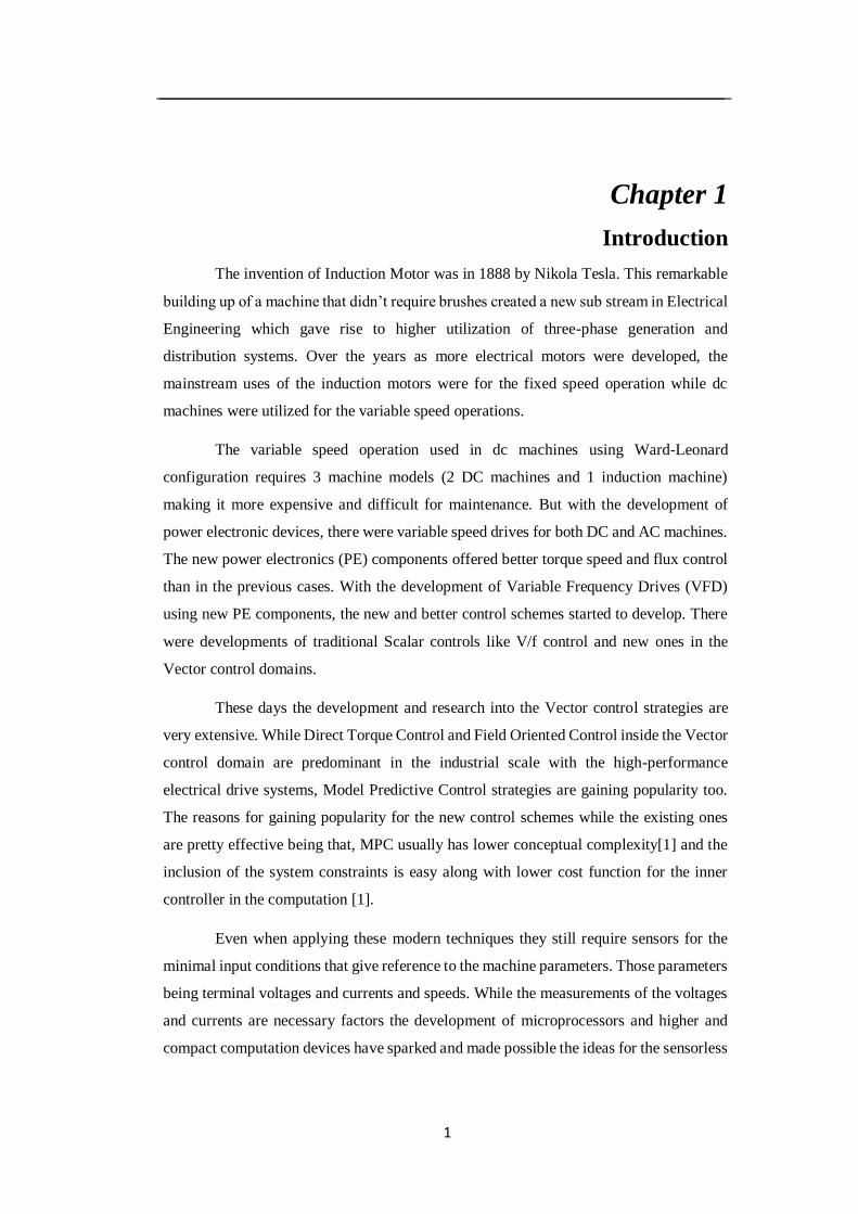
The invention of Induction Motor was in 1888 by Nikola Tesla. This remarkable

building up of a machine that didn’t require brushes created a new sub stream in Electrical

Engineering which gave rise to higher utilization of three-phase generation and

distribution systems. Over the years as more electrical motors were developed, the

mainstream uses of the induction motors were for the fixed speed operation while dc

machines were utilized for the variable speed operations.

The variable speed operation used in dc machines using Ward-Leonard

configuration requires 3 machine models (2 DC machines and 1 induction machine)

making it more expensive and difficult for maintenance. But with the development of

power electronic devices, there were variable speed drives for both DC and AC machines.

The new power electronics (PE) components offered better torque speed and flux control

than in the previous cases. With the development of Variable Frequency Drives (VFD)

using new PE components, the new and better control schemes started to develop. There

were developments of traditional Scalar controls like V/f control and new ones in the

Vector control domains.

These days the development and research into the Vector control strategies are

very extensive. While Direct Torque Control and Field Oriented Control inside the Vector

control domain are predominant in the industrial scale with the high-performance

electrical drive systems, Model Predictive Control strategies are gaining popularity too.

The reasons for gaining popularity for the new control schemes while the existing ones

are pretty effective being that, MPC usually has lower conceptual complexity[1] and the

inclusion of the system constraints is easy along with lower cost function for the inner

controller in the computation [1].

Even when applying these modern techniques they still require sensors for the

minimal input conditions that give reference to the machine parameters. Those parameters

being terminal voltages and currents and speeds. While the measurements of the voltages

and currents are necessary factors the development of microprocessors and higher and

compact computation devices have sparked and made possible the ideas for the sensorless

_______________________________________________________________________

2

speed determination techniques. The sensorless vector controls of motor drives refer

generally to the speed sensorless drives. The use of speed sensors is not always

environmentally friendly. They are prone to large shocks and other environmental

conditions [2]. The development of sensorless control and predictive analysis is effective

from the perspective of reliability, and maintainability. The sensorless controls are more

robust in contrast to the use of sensors in other methods. In addition to this, the economic

aspects of the sensorless controls are more desirable [3].

Primary aspects of the sensorless control are the estimation of the rotor speed

using predictive filter algorithms, and coupling the estimated speed with the MPC

strategies. In this thesis, we present the derivation, implementation and hardware

realization of one of such methods of sensorless control using Kalman Filter techniques,

in a laboratory motor and the comparison of such a filter response with the actual response

and the references given. The primary task discussed in this thesis includes the design and

implementation of the Kalman Filter and the reliability of the estimated speed, in

comparison with the actual motor speed and the reference speed. The further extension of

the estimated speed has been on the deployment of the sensorless vector control of the

motor. But the thesis primarily focusses on the estimation of the rotor speed. We are

starting with the mathematical modeling of the filter and the machine models used in this

thesis in Chapter 2. In Chapter 3, we will discuss the Simulation of the filter and the motor

model and control strategies in Matlab Simulink. Chapter 4 discusses the workplace setup

and the hardware assembled to realize the model verified in the simulations to the

laboratory. In Chapter 5 the various experimental results are analyzed. Chapter 6 is the

Conclusion for the thesis. Following sections after it is the References.

_______________________________________________________________________

3

Chapter 2

Kalman Filter and its Design for Induction Motor Speed

Determination

2.1 Kalman Filter:

The estimation of the rotor speed in this thesis focuses on the Kalman Filter and

Extended Kalman Filter. The Kalman Filter (KF) is a mathematical tool for estimation of

a state based on the previous state and the observed values of the noise like measurement

noise and the system noise and measured values – like outputs. They are primarily used in

prediction and estimation fields that include GPS operations, AI applications where

positioning and band of errors are significant, and unmanned operations like space and

military operations.

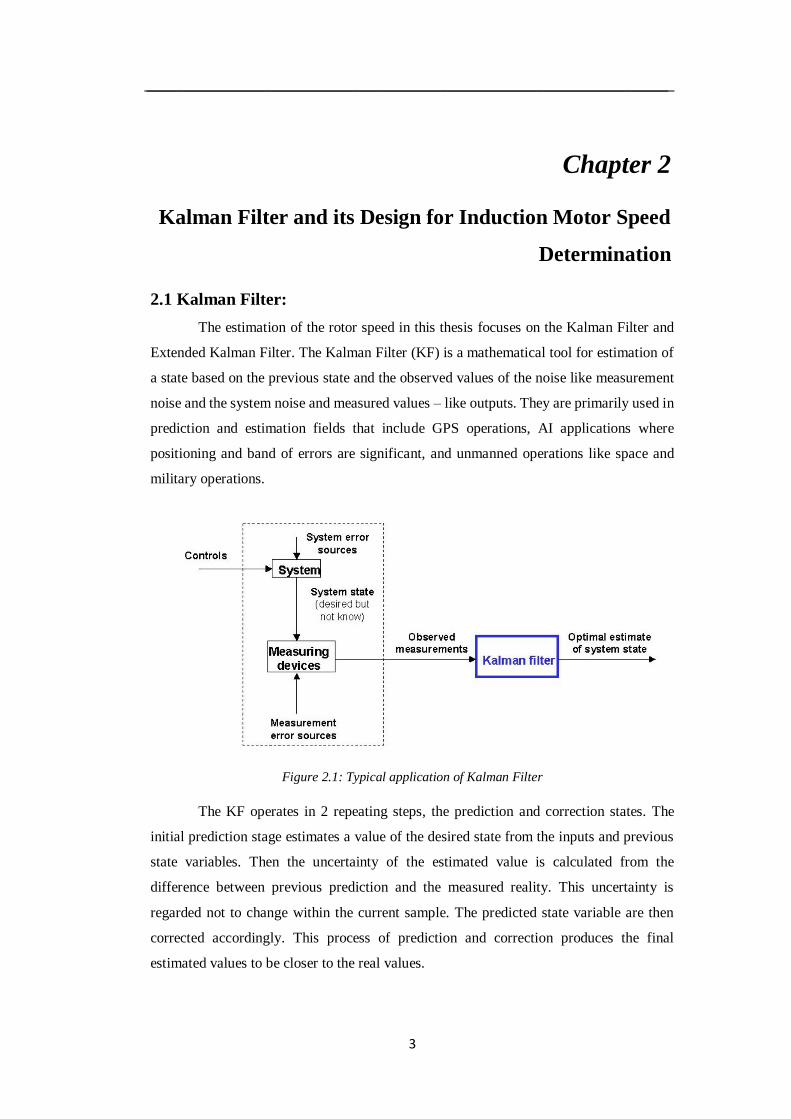
Figure 2.1: Typical application of Kalman Filter

The KF operates in 2 repeating steps, the prediction and correction states. The

initial prediction stage estimates a value of the desired state from the inputs and previous

state variables. Then the uncertainty of the estimated value is calculated from the

difference between previous prediction and the measured reality. This uncertainty is

regarded not to change within the current sample. The predicted state variable are then

corrected accordingly. This process of prediction and correction produces the final

estimated values to be closer to the real values.

_______________________________________________________________________

4

2.1.1 The Process to be estimated:

KF is used in the estimation of a discrete-time controlled process that is governed

by the linear stochastic difference equation. [4]

𝑥𝑘 = 𝐹𝑥𝑘−1 + 𝐵𝑘 𝑢𝑘−1 + 𝑣𝑘−1 (2.1)

And the output (observation) given by

𝑦𝑘 = 𝐻𝑘𝑥𝑘 + 𝑤𝑘 (2.2)

Where,

𝑝(𝑣) ~ 𝑁(0,𝑄) (2.3)

𝑝(𝑤) ~ 𝑁(0, 𝑅) (2.4)

Where, uk represents the input parameter or the control vector, Fk is the state transition

model, Bk is the control input model, and Hk is the observation model which maps the true

state space into the observed space or the output. The random variables wk and vk in

equations 2.1 and 2.2 represent the process and measurement noise respectively. The

noises are uncorrelated, assumed to be white noise with normal probability distributions.

The Q and R are the system noise covariance matrix and measurement noise covariance

matrix. While they are changing constantly in every time step and measurement, it is

assumed that they are constant matrices. [4]

2.1.2 The Estimation Process:

Like we described earlier the filtering process occurs over two stages: prediction

and correction. The initial conditions for the first stage are given with the prior knowledge

of the process to be estimated or state as we would call it here forward, and the state

covariance matrix of prediction (P). The first stage initializes the state vectors and the

covariance matrices, then the preliminary prediction of the state vector and the covariance

matrix of prediction. On the second stage of the loop, which is the correction stage, the

measurement noise covariance matrices come into play. Initially, the Kalman Gain is

computed based on the predicted P in the first stage, along with the inclusion of

measurement noise in the equation. After the calculation of the Kalman Gain, the state

vector predicted in the first stage are corrected based on the error factor developed from

the difference of the measured and predicted outcome values. Then the correction of the

covariance matrix of prediction is done for the next loop which acts as the initial condition

_______________________________________________________________________

5

for the next loop. In this way, the 2 stage loop cycle runs to give an estimate for any

discrete-time controlled process governed by the linear stochastic difference equation.[4]

2.1.3 Mathematical Representation:

Predict:

Predicted State: 𝑘|𝑘−1 = 𝐹𝑘𝑘−1|𝑘−1 + 𝐵𝑘 𝑢𝑘 (2.5)

Covariance of Prediction 𝑃𝑘|𝑘−1 = 𝐹𝑘𝑃𝑘−1|𝑘−1𝐹𝑘𝑇 + 𝑄𝑘 (2.6)

Update:

Kalman Gain Computation: 𝐾𝑘 = 𝑃𝑘|𝑘−1𝐻𝑘𝑇(𝐻𝑘𝑃𝑘|𝑘−1𝐻𝑘

𝑇 + 𝑅𝑘)−1 (2.7)

Measurement residual: 𝑘 = 𝑦𝑘 − 𝐻𝑘𝑘|𝑘−1 (2.8)

Updated state estimate: 𝑘|𝑘 = 𝑘|𝑘−1 + 𝐾𝑘𝑘 (2.9)

Updated Covariance of Prediction 𝑃𝑘|𝑘 = (𝐼 − 𝐾𝑘𝐻𝑘) 𝑃𝑘|𝑘−1 (2.10)

2.2 Extended Kalman Filter:

The Kalman Filter discusses above is only valid for linear functions, while most

of the real systems are governed by non-linear functions. The Extended Kalman Filter

(EKF) is the nonlinear version of the Kalman Filter. It linearizes about the current mean

and covariance. [5] While EKF had been used extensively as a standard tool for estimation

of nonlinear states in navigation systems and GPS, with the introduction of Unscented

Kalman Filter the extensive use has reduced. [6]

In the modeling of the filter in this thesis, the Extended Kalman Filter algorithm has been

used. The difference in the formulation of the EKF in comparison to KF is such that the

state transition and observation state space models may not be linear functions of the state

but are often many nonlinear functions. [7]

𝑥𝑘 = 𝑓(𝑥𝑘−1, 𝑢𝑘) + 𝑣𝑘 (2.11)

𝑦𝑘 = ℎ(𝑥𝑘) + 𝑤𝑘 (2.12)

Like in the previous case with KF the random variables vk and wk are the system

and measurement noises, which are both assumed to be zero mean multivariate Gaussian

noise with covariance Qk and Rk respectively. The vector uk is the input control vector.

_______________________________________________________________________

6

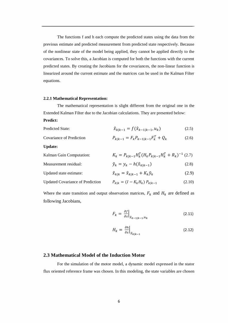
The functions f and h each compute the predicted states using the data from the

previous estimate and predicted measurement from predicted state respectively. Because

of the nonlinear state of the model being applied, they cannot be applied directly to the

covariances. To solve this, a Jacobian is computed for both the functions with the current

predicted states. By creating the Jacobians for the covariances, the non-linear function is

linearized around the current estimate and the matrices can be used in the Kalman Filter

equations.

2.2.1 Mathematical Representation:

The mathematical representation is slight different from the original one in the

Extended Kalman Filter due to the Jacobian calculations. They are presented below:

Predict:

Predicted State: 𝑘|𝑘−1 = 𝑓(𝑘−1|𝑘−1, 𝑢𝑘) (2.5)

Covariance of Prediction 𝑃𝑘|𝑘−1 = 𝐹𝑘𝑃𝑘−1|𝑘−1𝐹𝑘𝑇 + 𝑄𝑘 (2.6)

Update:

Kalman Gain Computation: 𝐾𝑘 = 𝑃𝑘|𝑘−1𝐻𝑘𝑇(𝐻𝑘𝑃𝑘|𝑘−1𝐻𝑘

𝑇 + 𝑅𝑘)−1 (2.7)

Measurement residual: 𝑘 = 𝑦𝑘 − ℎ(𝑘|𝑘−1) (2.8)

Updated state estimate: 𝑘|𝑘 = 𝑘|𝑘−1 + 𝐾𝑘𝑘 (2.9)

Updated Covariance of Prediction 𝑃𝑘|𝑘 = (𝐼 − 𝐾𝑘𝐻𝑘) 𝑃𝑘|𝑘−1 (2.10)

Where the state transition and output observation matrices, 𝐹𝑘 and 𝐻𝑘 are defined as

following Jacobians,

𝐹𝑘 = 𝜕𝑓

𝜕𝑥|𝑥𝑘−1|𝑘−1,𝑢𝑘

(2.11)

𝐻𝑘 = 𝜕ℎ

𝜕𝑥|𝑥𝑘|𝑘−1

(2.12)

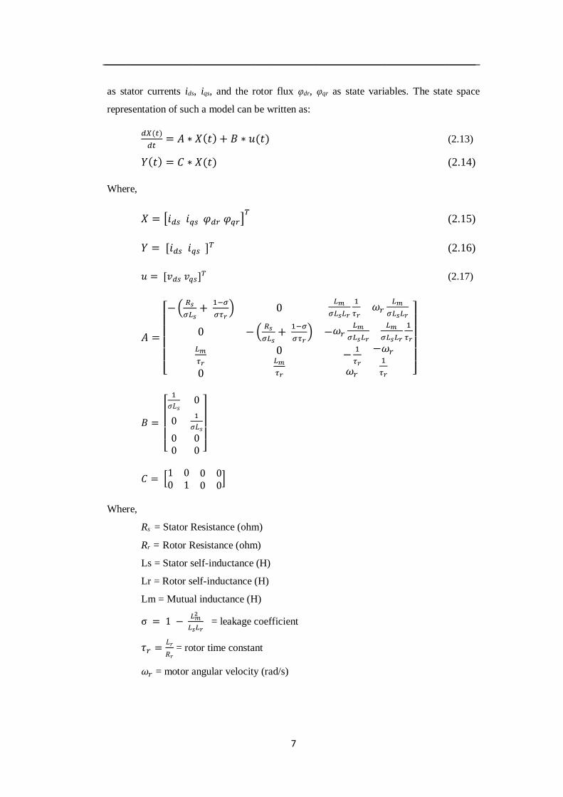
2.3 Mathematical Model of the Induction Motor

For the simulation of the motor model, a dynamic model expressed in the stator

flux oriented reference frame was chosen. In this modeling, the state variables are chosen

_______________________________________________________________________

7

as stator currents ids, iqs, and the rotor flux φdr, φqr as state variables. The state space

representation of such a model can be written as:

𝑑𝑋(𝑡)

𝑑𝑡= 𝐴 ∗ 𝑋(𝑡) + 𝐵 ∗ 𝑢(𝑡) (2.13)

𝑌(𝑡) = 𝐶 ∗ 𝑋(𝑡) (2.14)

Where,

𝑋 = [𝑖𝑑𝑠 𝑖𝑞𝑠 𝜑𝑑𝑟 𝜑𝑞𝑟]𝑇 (2.15)

𝑌 = [𝑖𝑑𝑠 𝑖𝑞𝑠 ]𝑇 (2.16)

𝑢 = [𝑣𝑑𝑠 𝑣𝑞𝑠]𝑇 (2.17)

𝐴 =

[ −(

𝑅𝑠

𝜎𝐿𝑠+

1−𝜎

𝜎𝜏𝑟) 0

𝐿𝑚

𝜎𝐿𝑠𝐿𝑟

1

𝜏𝑟𝜔𝑟

𝐿𝑚

𝜎𝐿𝑠𝐿𝑟

0 − (𝑅𝑠

𝜎𝐿𝑠+

1−𝜎

𝜎𝜏𝑟) −𝜔𝑟

𝐿𝑚

𝜎𝐿𝑠𝐿𝑟

𝐿𝑚

𝜎𝐿𝑠𝐿𝑟

1

𝜏𝑟

𝐿𝑚

𝜏𝑟

0

0𝐿𝑚

𝜏𝑟

−1

𝜏𝑟

𝜔𝑟

−𝜔𝑟1

𝜏𝑟 ]

𝐵 =

[

1

𝜎𝐿𝑠0

01

𝜎𝐿𝑠

00

00 ]

𝐶 = [1 0 0 00 1 0 0

]

Where,

Rs = Stator Resistance (ohm)

Rr = Rotor Resistance (ohm)

Ls = Stator self-inductance (H)

Lr = Rotor self-inductance (H)

Lm = Mutual inductance (H)

σ = 1 − 𝐿𝑚2

𝐿𝑠𝐿𝑟 = leakage coefficient

𝜏𝑟 =𝐿𝑟

𝑅𝑟 = rotor time constant

𝜔𝑟 = motor angular velocity (rad/s)

_______________________________________________________________________

8

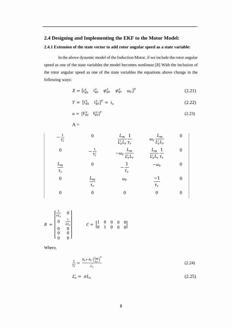
2.4 Designing and Implementing the EKF to the Motor Model:

2.4.1 Extension of the state vector to add rotor angular speed as a state variable:

In the above dynamic model of the Induction Motor, if we include the rotor angular

speed as one of the state variables the model becomes nonlinear.[8] With the inclusion of

the rotor angular speed as one of the state variables the equations above change in the

following ways:

𝑋 = [𝑖𝑑𝑠𝑠 𝑖𝑞𝑠

𝑠 𝜑𝑑𝑟𝑠 𝜑𝑞𝑟

𝑠 𝜔𝑟]𝑇 (2.21)

𝑌 = [𝑖𝑑𝑠𝑠 𝑖𝑞𝑠

𝑠 ]𝑇 = 𝑖𝑠 (2.22)

𝑢 = [𝑉𝑑𝑠𝑠 𝑉𝑞𝑠

𝑠 ]𝑇 (2.23)

A =

−1

𝑇𝑠∗

0 𝐿𝑚

𝐿𝑠′ 𝐿𝑟

1

𝜏𝑟 𝜔𝑟

𝐿𝑚

𝐿𝑠′ 𝐿𝑟

0

0 −1

𝑇𝑠∗ −𝜔𝑟

𝐿𝑚

𝐿𝑠′ 𝐿𝑟

𝐿𝑚

𝐿𝑠′ 𝐿𝑟

1

𝜏𝑟

0

𝐿𝑚

𝜏𝑟

0 −

1

𝜏𝑟

−𝜔𝑟 0

0 𝐿𝑚

𝜏𝑟

𝜔𝑟 −1

𝜏𝑟

0

0 0 0 0 0

𝐵 =

[

1

𝜎𝐿𝑠0

01

𝜎𝐿𝑠

000

000 ]

𝐶 = [1 0 0 0 00 1 0 0 0

]

Where,

1

𝑇𝑠∗ =

𝑅𝑠+ 𝑅𝑟 (𝐿𝑚𝐿𝑟

)2

𝐿𝑠′ (2.24)

𝐿𝑠′ = 𝜎𝐿𝑠 (2.25)

_______________________________________________________________________

9

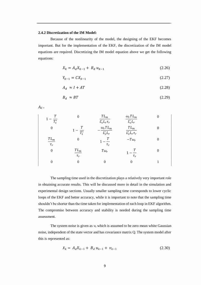
2.4.2 Discretization of the IM Model:

Because of the nonlinearity of the model, the designing of the EKF becomes

important. But for the implementation of the EKF, the discretization of the IM model

equations are required. Discretizing the IM model equation above we get the following

equations:

𝑋𝑘 = 𝐴𝑑𝑋𝑘−1 + 𝐵𝑑 𝑢𝑘−1 (2.26)

𝑌𝑘−1 = 𝐶𝑋𝑘−1 (2.27)

𝐴𝑑 ≈ 𝐼 + 𝐴𝑇 (2.28)

𝐵𝑑 ≈ 𝐵𝑇 (2.29)

Ad =

1 − 𝑇

𝑇𝑠∗

0 𝑇𝐿𝑚

𝐿𝑠′ 𝐿𝑟𝜏𝑟

𝜔𝑟𝑇𝐿𝑚

𝐿𝑠′ 𝐿𝑟

0

0 1 −

𝑇

𝑇𝑠∗ −

𝜔𝑟𝑇𝐿𝑚

𝐿𝑠′ 𝐿𝑟

𝑇𝐿𝑚

𝐿𝑠′ 𝐿𝑟𝜏𝑟

0

𝑇𝐿𝑚

𝜏𝑟

0 1 −

𝑇

𝜏𝑟

−𝑇𝜔𝑟 0

0 𝑇𝐿𝑚

𝜏𝑟

𝑇𝜔𝑟 1 −

𝑇

𝜏𝑟

0

0 0 0 0 1

The sampling time used in the discretization plays a relatively very important role

in obtaining accurate results. This will be discussed more in detail in the simulation and

experimental design sections. Usually smaller sampling time corresponds to lower cyclic

loops of the EKF and better accuracy, while it is important to note that the sampling time

shouldn’t be shorter than the time taken for implementation of each loop in EKF algorithm.

The compromise between accuracy and stability is needed during the sampling time

assessment.

The system noise is given as vk which is assumed to be zero mean white Gaussian

noise, independent of the state vector and has covariance matrix Q. The system model after

this is represented as:

𝑋𝑘 = 𝐴𝑑𝑋𝑘−1 + 𝐵𝑑 𝑢𝑘−1 + 𝑣𝑘−1 (2.30)

_______________________________________________________________________

10

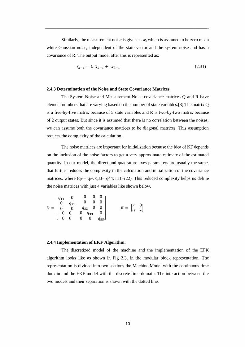
Similarly, the measurement noise is given as wk which is assumed to be zero mean

white Gaussian noise, independent of the state vector and the system noise and has a

covariance of R. The output model after this is represented as:

𝑌𝑘−1 = 𝐶 𝑋𝑘−1 + 𝑤𝑘−1 (2.31)

2.4.3 Determination of the Noise and State Covariance Matrices

The System Noise and Measurement Noise covariance matrices Q and R have

element numbers that are varying based on the number of state variables.[8] The matrix Q

is a five-by-five matrix because of 5 state variables and R is two-by-two matrix because

of 2 output states. But since it is assumed that there is no correlation between the noises,

we can assume both the covariance matrices to be diagonal matrices. This assumption

reduces the complexity of the calculation.

The noise matrices are important for initialization because the idea of KF depends

on the inclusion of the noise factors to get a very approximate estimate of the estimated

quantity. In our model, the direct and quadrature axes parameters are usually the same,

that further reduces the complexity in the calculation and initialization of the covariance

matrices, where (q11= q22, q33= q44, r11=r22). This reduced complexity helps us define

the noise matrices with just 4 variables like shown below.

𝑄 =

[ 𝑞11 00 𝑞11

0 000

00

0 0 00 0 0

𝑞33 0 00 𝑞33 00 0 𝑞55]

𝑅 = [𝑟 00 𝑟

]

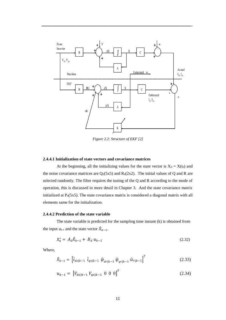
2.4.4 Implementation of EKF Algorithm:

The discretized model of the machine and the implementation of the EFK

algorithm looks like as shown in Fig 2.3, in the modular block representation. The

representation is divided into two sections the Machine Model with the continuous time

domain and the EKF model with the discrete time domain. The interaction between the

two models and their separation is shown with the dotted line.

_______________________________________________________________________

11

Figure 2.2: Structure of EKF [2]

2.4.4.1 Initialization of state vectors and covariance matrices

At the beginning, all the initializing values for the state vector is X0 = X(t0) and

the noise covariance matrices are Q0(5x5) and R0(2x2). The initial values of Q and R are

selected randomly. The filter requires the tuning of the Q and R according to the mode of

operation, this is discussed in more detail in Chapter 3. And the state covariance matrix

initialized at P0(5x5). The state covariance matrix is considered a diagonal matrix with all

elements same for the initialization.

2.4.4.2 Prediction of the state variable

The state variable is predicted for the sampling time instant (k) is obtained from

the input uk-1 and the state vector 𝑘−1.

𝑋𝑘∗ = 𝐴𝑑𝑘−1 + 𝐵𝑑 𝑢𝑘−1 (2.32)

Where,

𝑘−1 = [𝑑𝑠|𝑘−1 𝑞𝑠|𝑘−1 𝑑𝑟|𝑘−1

𝑞𝑟|𝑘−1 𝑟|𝑘−1]

𝑇 (2.33)

𝑢𝑘−1 = [𝑉𝑑𝑠|𝑘−1 𝑉𝑞𝑠|𝑘−1 0 0 0]𝑇 (2.34)

_______________________________________________________________________

12

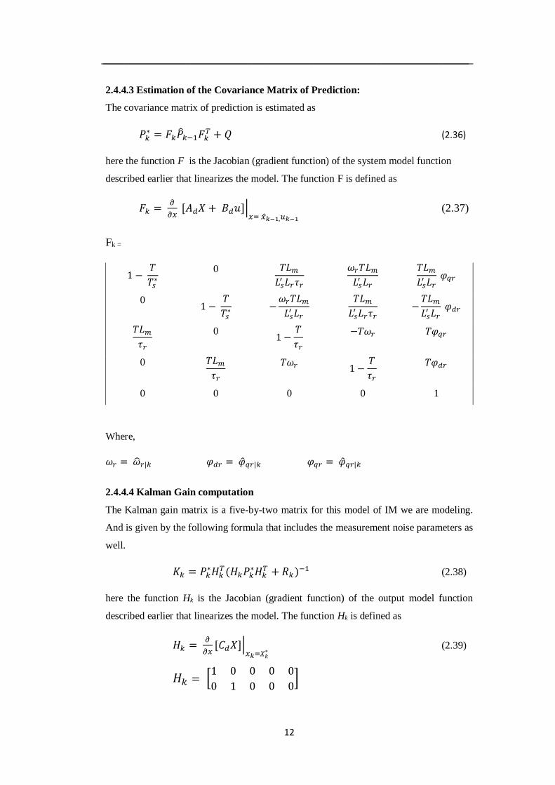
2.4.4.3 Estimation of the Covariance Matrix of Prediction:

The covariance matrix of prediction is estimated as

𝑃𝑘∗ = 𝐹𝑘𝑘−1𝐹𝑘

𝑇 + 𝑄 (2.36)

here the function F is the Jacobian (gradient function) of the system model function

described earlier that linearizes the model. The function F is defined as

𝐹𝑘 = 𝜕

𝜕𝑥 [𝐴𝑑𝑋 + 𝐵𝑑𝑢]|

𝑥= 𝑥𝑘−1,𝑢𝑘−1

(2.37)

Fk =

1 − 𝑇

𝑇𝑠∗

0 𝑇𝐿𝑚

𝐿𝑠′ 𝐿𝑟𝜏𝑟

𝜔𝑟𝑇𝐿𝑚

𝐿𝑠′ 𝐿𝑟

𝑇𝐿𝑚

𝐿𝑠′ 𝐿𝑟

𝜑𝑞𝑟

0 1 −

𝑇

𝑇𝑠∗ −

𝜔𝑟𝑇𝐿𝑚

𝐿𝑠′ 𝐿𝑟

𝑇𝐿𝑚

𝐿𝑠′ 𝐿𝑟𝜏𝑟

−𝑇𝐿𝑚

𝐿𝑠′ 𝐿𝑟

𝜑𝑑𝑟

𝑇𝐿𝑚

𝜏𝑟

0 1 −

𝑇

𝜏𝑟

−𝑇𝜔𝑟 𝑇𝜑𝑞𝑟

0 𝑇𝐿𝑚

𝜏𝑟

𝑇𝜔𝑟 1 −

𝑇

𝜏𝑟

𝑇𝜑𝑑𝑟

0 0 0 0 1

Where,

𝜔𝑟 = 𝑟|𝑘 𝜑𝑑𝑟 = 𝑞𝑟|𝑘 𝜑𝑞𝑟 = 𝑞𝑟|𝑘

2.4.4.4 Kalman Gain computation

The Kalman gain matrix is a five-by-two matrix for this model of IM we are modeling.

And is given by the following formula that includes the measurement noise parameters as

well.

𝐾𝑘 = 𝑃𝑘∗𝐻𝑘

𝑇(𝐻𝑘𝑃𝑘∗𝐻𝑘

𝑇 + 𝑅𝑘)−1 (2.38)

here the function Hk is the Jacobian (gradient function) of the output model function

described earlier that linearizes the model. The function Hk is defined as

𝐻𝑘 = 𝜕

𝜕𝑥[𝐶𝑑𝑋]|

𝑥𝑘=𝑋𝑘∗

(2.39)

𝐻𝑘 = [1 0 0 0 0

0 1 0 0 0]

_______________________________________________________________________

13

2.4.4.5 State Vector Estimation:

The final estimated state vector and the output models after the filtering at time

(k+1) is given as:

𝑘 = 𝑋𝑘∗ + 𝐾𝑘𝑘 (2.40)

𝑘 = 𝑌𝑘 − 𝑘 (2.41)

𝑘 = 𝐶𝑑 𝑋𝑘∗ (2.42)

2.4.4.6 Correction of the Covariance Matrix of Prediction for next loop:

The error covariance matrix is obtained from

𝑘 = 𝑃𝑘∗ − 𝐾𝑘 𝐻𝑘𝑃𝑘

∗ (2.43)

With the last step the loop ends for 1 cycle, for the next sampling time instant that

is k+1, now the values in the loop are updated by putting k = k+1, and repeating the process

from 2.4.4.2 to 2.4.4.6.

_______________________________________________________________________

14

Chapter 3

Simulation of IM and EKF in Simulink Matlab

In the previous chapter, we developed the mathematical modeling of the EKF and

the IM equations for the estimation of the rotor speed. In this chapter, we will continue

with mapping those equations into the Matlab Simulink and look at the preliminary

simulation results.

3.1 Model of IM and Control Strategy:

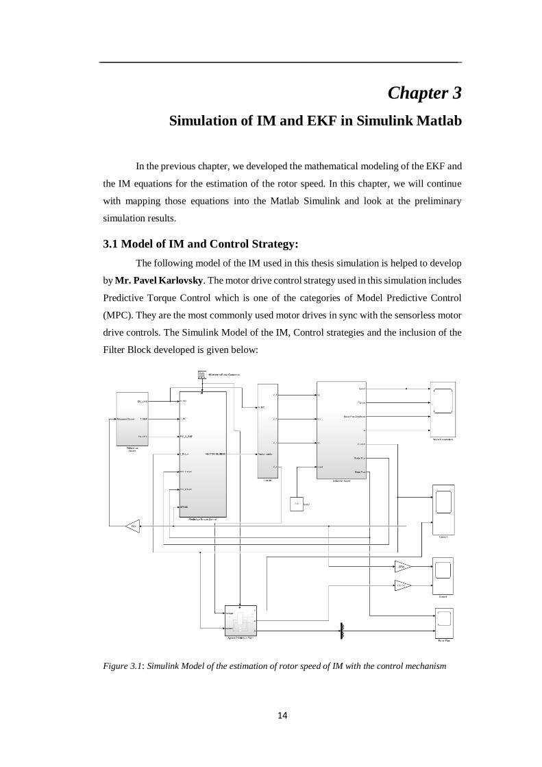
The following model of the IM used in this thesis simulation is helped to develop

by Mr. Pavel Karlovsky. The motor drive control strategy used in this simulation includes

Predictive Torque Control which is one of the categories of Model Predictive Control

(MPC). They are the most commonly used motor drives in sync with the sensorless motor

drive controls. The Simulink Model of the IM, Control strategies and the inclusion of the

Filter Block developed is given below:

Figure 3.1: Simulink Model of the estimation of rotor speed of IM with the control mechanism

_______________________________________________________________________

15

The major blocks in this simulation include the Reference Block, Predictive

Torque Control Block, Inverter Block, Induction Motor Block (from left to right on Figure

4.1 on the top shelf) and the EKF block at the bottom. Each of the Blocks internal

schematic are discussed ahead.

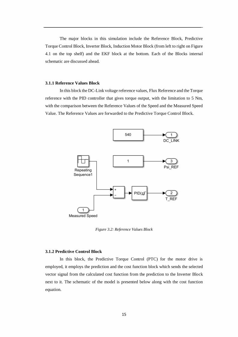
3.1.1 Reference Values Block

In this block the DC-Link voltage reference values, Flux Reference and the Torque

reference with the PID controller that gives torque output, with the limitation to 5 Nm,

with the comparison between the Reference Values of the Speed and the Measured Speed

Value. The Reference Values are forwarded to the Predictive Torque Control Block.

Figure 3.2: Reference Values Block

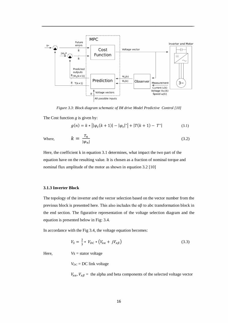
3.1.2 Predictive Control Block

In this block, the Predictive Torque Control (PTC) for the motor drive is

employed, it employs the prediction and the cost function block which sends the selected

vector signal from the calculated cost function from the prediction to the Inverter Block

next to it. The schematic of the model is presented below along with the cost function

equation.

_______________________________________________________________________

16

Figure 3.3: Block diagram schematic of IM drive Model Predictive Control [10]

The Cost function g is given by:

𝑔(𝑛) = 𝑘 ∗ ||𝜑𝑠(𝑘 + 1)| − |𝜑𝑠|∗| + |𝑇(𝑘 + 1) − 𝑇∗| (3.1)

Where, 𝑘 = 𝑇𝑛

|𝜑𝑛| (3.2)

Here, the coefficient k in equation 3.1 determines, what impact the two part of the

equation have on the resulting value. It is chosen as a fraction of nominal torque and

nominal flux amplitude of the motor as shown in equation 3.2 [10]

3.1.3 Inverter Block

The topology of the inverter and the vector selection based on the vector number from the

previous block is presented here. This also includes the αβ to abc transformation block in

the end section. The figurative representation of the voltage selection diagram and the

equation is presented below in Fig: 3.4.

In accordance with the Fig 3.4, the voltage equation becomes:

𝑉𝑆 = 2

3∗ 𝑉𝐷𝐶 ∗ (𝑉𝑥𝛼 + 𝑗𝑉𝑥𝛽) (3.3)

Here, Vs = stator voltage

VDC = DC link voltage

𝑉𝑥𝛼 , 𝑉𝑥𝛽 = the alpha and beta components of the selected voltage vector

_______________________________________________________________________

17

Figure 3.4: Voltage vector diagram

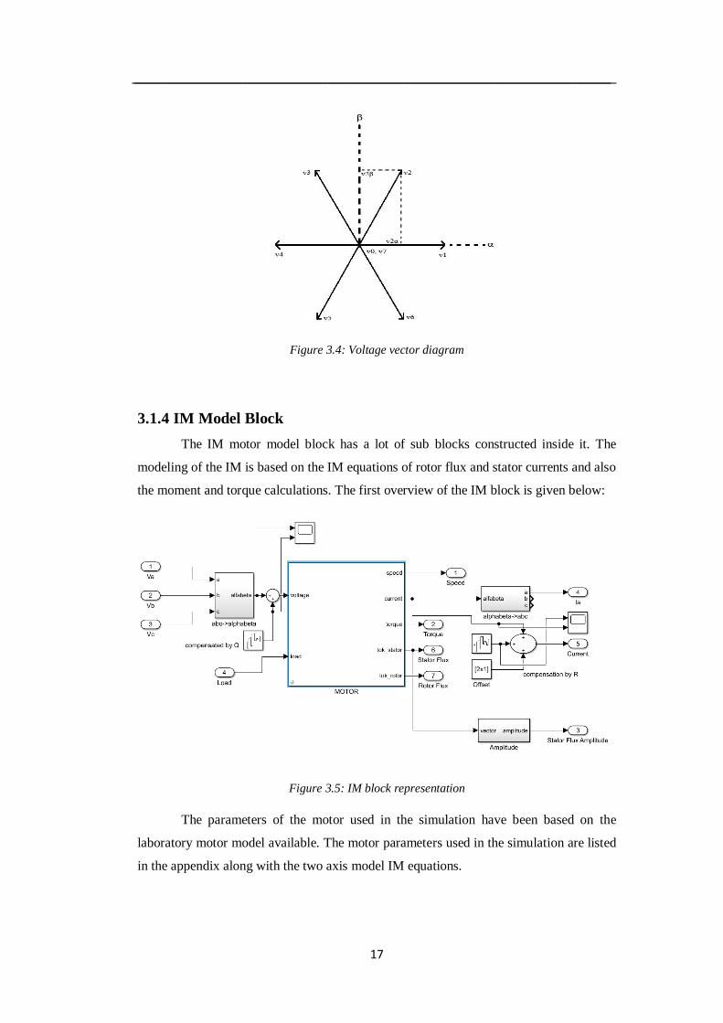
3.1.4 IM Model Block

The IM motor model block has a lot of sub blocks constructed inside it. The

modeling of the IM is based on the IM equations of rotor flux and stator currents and also

the moment and torque calculations. The first overview of the IM block is given below:

Figure 3.5: IM block representation

The parameters of the motor used in the simulation have been based on the

laboratory motor model available. The motor parameters used in the simulation are listed

in the appendix along with the two axis model IM equations.

_______________________________________________________________________

18

3.2 EKF Model

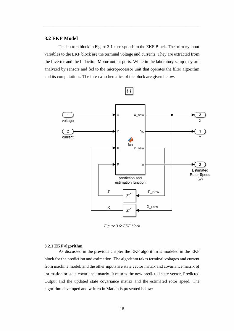
The bottom block in Figure 3.1 corresponds to the EKF Block. The primary input

variables to the EKF block are the terminal voltage and currents. They are extracted from

the Inverter and the Induction Motor output ports. While in the laboratory setup they are

analyzed by sensors and fed to the microprocessor unit that operates the filter algorithm

and its computations. The internal schematics of the block are given below.

Figure 3.6: EKF block

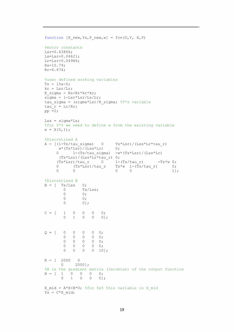
3.2.1 EKF algorithm

As discussed in the previous chapter the EKF algorithm is modeled in the EKF

block for the prediction and estimation. The algorithm takes terminal voltages and current

from machine model, and the other inputs are state vector matrix and covariance matrix of

estimation or state covariance matrix. It returns the new predicted state vector, Predicted

Output and the updated state covariance matrix and the estimated rotor speed. The

algorithm developed and written in Matlab is presented below:

_______________________________________________________________________

19

function [X_new,Ys,P_new,w] = fcn(U,Y, X,P)

%motor constants Lsr=0.63866; Ls=Lsr+0.04621; Lr=Lsr+0.04986; Rs=10.79; Rr=6.674;

%user defined working variables Ts = 15e-5; kr = Lsr/Lr; R_sigma = Rs+Rr*kr*kr; sigma = 1-Lsr*Lsr/Ls/Lr; tau_sigma = (sigma*Ls)/R_sigma; %T*s variable tau_r = Lr/Rr; pp =2;

Lss = sigma*Ls;

%for 5*5 we need to define w from the existing variable w = X(5,1);

%Discretized A A = [(1-Ts/tau_sigma) 0 Ts*Lsr)/(Lss*Lr*tau_r)

w*(Ts*Lsr)/(Lss*Lr) 0; 0 1-(Ts/tau_sigma) -w*(Ts*Lsr)/(Lss*Lr)

(Ts*Lsr)/(Lss*Lr*tau_r) 0; (Ts*Lsr)/tau_r 0 1-(Ts/tau_r) -Ts*w 0; 0 (Ts*Lsr)/tau_r Ts*w 1-(Ts/tau_r) 0; 0 0 0 0 1];

%Discretized B B = [ Ts/Lss 0; 0 Ts/Lss; 0 0; 0 0; 0 0];

C = [ 1 0 0 0 0; 0 1 0 0 0];

Q = [ 0 0 0 0 0; 0 0 0 0 0; 0 0 0 0 0; 0 0 0 0 0; 0 0 0 0 10];

R = [ 2000 0 0 2000]; %H is the gradient matrix (Jacobian) of the output function H = [ 1 0 0 0 0; 0 1 0 0 0];

X_mid = A*X+B*U; %for 5x5 this variable is X_mid Ys = C*X_mid;

_______________________________________________________________________

20

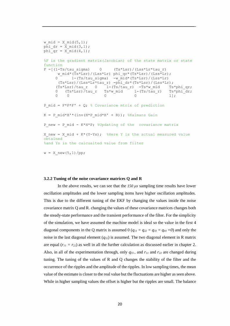
w_mid = X_mid(5,1); phi_dr = X_mid(3,1); phi_qr = X_mid(4,1);

%F is the gradient matrix(Jacobian) of the state matrix or state

function F =[(1-Ts/tau_sigma) 0 (Ts*Lsr)/(Lss*Lr*tau_r)

w_mid*(Ts*Lsr)/(Lss*Lr) phi_qr*(Ts*Lsr)/(Lss*Lr); 0 1-(Ts/tau_sigma) -w_mid*(Ts*Lsr)/(Lss*Lr)

(Ts*Lsr)/(Lss*Lr*tau_r) -phi_dr*(Ts*Lsr)/(Lss*Lr); (Ts*Lsr)/tau_r 0 1-(Ts/tau_r) -Ts*w_mid Ts*phi_qr; 0 (Ts*Lsr)/tau_r Ts*w_mid 1-(Ts/tau_r) Ts*phi_dr; 0 0 0 0 1];

P_mid = F*P*F' + Q; % Covariance mtrix of prediction

K = P_mid*H'*(inv(H*P_mid*H' + R)); %Kalmans Gain

P_new = P_mid - K*H*P; %Updating of the covariance matrix

X_new = X_mid + K*(Y-Ys); %Here Y is the actual measured value

obtained %and Ys is the calcualted value from filter

w = X_new(5,1)/pp;

3.2.2 Tuning of the noise covariance matrices Q and R

In the above results, we can see that the 150 μs sampling time results have lower

oscillation amplitudes and the lower sampling items have higher oscillation amplitudes.

This is due to the different tuning of the EKF by changing the values inside the noise

covariance matrix Q and R. changing the values of these covariance matrices changes both

the steady-state performance and the transient performance of the filter. For the simplicity

of the simulation, we have assumed the machine model is ideal so the value in the first 4

diagonal components in the Q matrix is assumed 0 (q11 = q22 = q33 = q44 =0) and only the

noise in the last diagonal element (q55) is assumed. The two diagonal element in R matrix

are equal (r11 = r22) as well in all the further calculation as discussed earlier in chapter 2.

Also, in all of the experimentation through, only q55 , and r11 and r22 are changed during

tuning. The tuning of the values of R and Q changes the stability of the filter and the

occurrence of the ripples and the amplitude of the ripples. In low sampling times, the mean

value of the estimate is closer to the real value but the fluctuations are higher as seen above.

While in higher sampling values the offset is higher but the ripples are small. The balance

_______________________________________________________________________

21

between the stability and the oscillations has to be selected. Between the values of Q and

R, the change in Q denotes the uncertainty in the machine model used and R denotes the

level of noise in the measurements. Higher Q corresponds to higher uncertainty in the

machine model used hence higher system noise. Higher R corresponds to higher

measurement noise, and the filter subjects them to less weight during computation. Hence

higher R causes longer computation time, making the transient performance slower. The

matrices have been tuned on various cases accordingly, based on the sampling time used

and the machine performance being observed is a transient response or steady state.

3.3 Simulation Results from Matlab Simulink

The simulation of the above model and the filter algorithm for the parameters of

the laboratory IM is done. The simulation was done for multiple sampling times (20 μs,

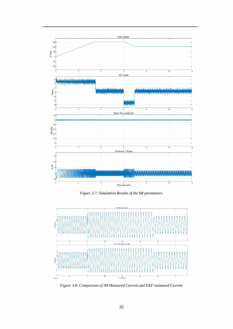
and 150 μs). The simulation results are presented below. Figure 3.7 shows the graphical

representation of the induction motor run over time, as we start the motor from a standstill

and take it to 1500rpm. At 6s, the motor stands to decelerate from 1500rpm to reach rotor

speed of 1000rpm. The variations in the rotor speed, the torque generated by the motor,

Stator flux amplitude and one of the phase currents is seen. Because the simulated was

tried to represent as much as the real model the addition of white noise to both current and

voltages have been done in the simulations both at 10% of the peak levels of individual

quantities respectively and relatively high offset level of 1A was added accordingly.

Figure 3.8 shows the simulation results of the EKF predicted output current

compared to the current from the IM. In both cases, only one of the phases is shown for

graphical clarity.

_______________________________________________________________________

22

Figure 3.7: Simulation Results of the IM parameters.

Figure 3.8: Comparison of IM Measured Current and EKF estimated Current

_______________________________________________________________________

23

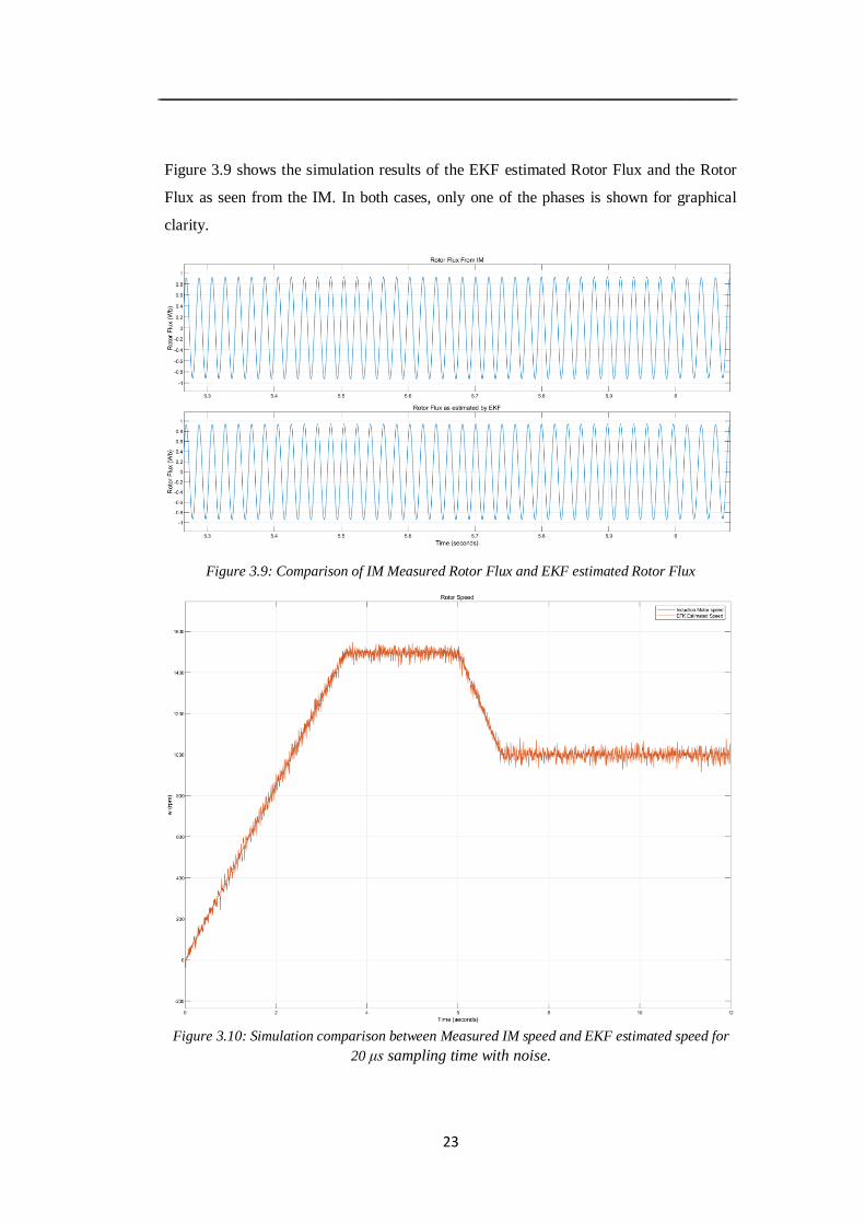
Figure 3.9 shows the simulation results of the EKF estimated Rotor Flux and the Rotor

Flux as seen from the IM. In both cases, only one of the phases is shown for graphical

clarity.

Figure 3.9: Comparison of IM Measured Rotor Flux and EKF estimated Rotor Flux

Figure 3.10: Simulation comparison between Measured IM speed and EKF estimated speed for

20 μs sampling time with noise.

_______________________________________________________________________

24

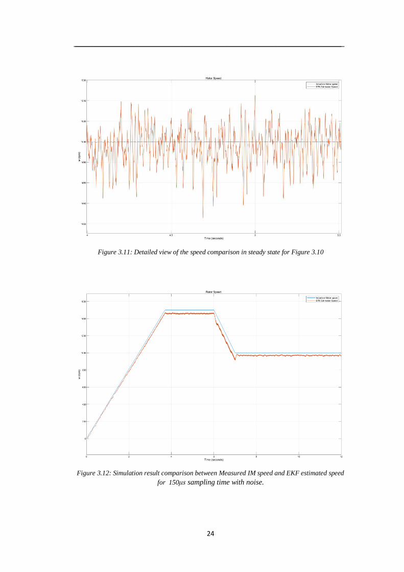
Figure 3.11: Detailed view of the speed comparison in steady state for Figure 3.10

Figure 3.12: Simulation result comparison between Measured IM speed and EKF estimated speed

for 150μs sampling time with noise.

_______________________________________________________________________

25

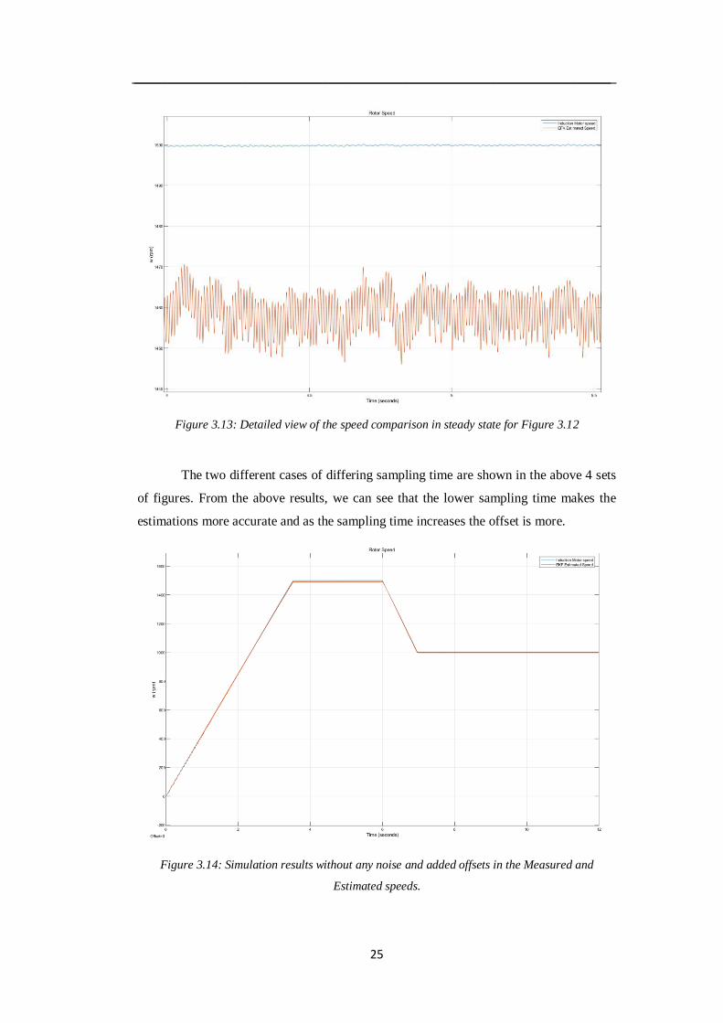
Figure 3.13: Detailed view of the speed comparison in steady state for Figure 3.12

The two different cases of differing sampling time are shown in the above 4 sets

of figures. From the above results, we can see that the lower sampling time makes the

estimations more accurate and as the sampling time increases the offset is more.

Figure 3.14: Simulation results without any noise and added offsets in the Measured and

Estimated speeds.

_______________________________________________________________________

26

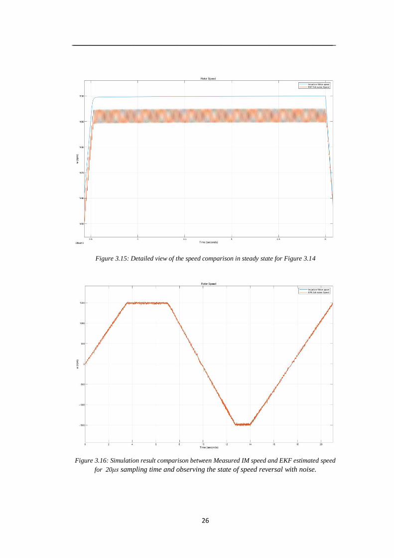
Figure 3.15: Detailed view of the speed comparison in steady state for Figure 3.14

Figure 3.16: Simulation result comparison between Measured IM speed and EKF estimated speed

for 20μs sampling time and observing the state of speed reversal with noise.

_______________________________________________________________________

27

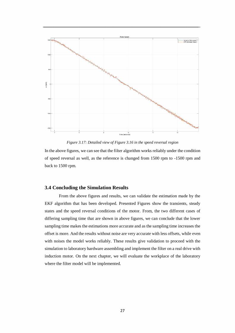
Figure 3.17: Detailed view of Figure 3.16 in the speed reversal region

In the above figures, we can see that the filter algorithm works reliably under the condition

of speed reversal as well, as the reference is changed from 1500 rpm to -1500 rpm and

back to 1500 rpm.

3.4 Concluding the Simulation Results

From the above figures and results, we can validate the estimation made by the

EKF algorithm that has been developed. Presented Figures show the transients, steady

states and the speed reversal conditions of the motor. From, the two different cases of

differing sampling time that are shown in above figures, we can conclude that the lower

sampling time makes the estimations more accurate and as the sampling time increases the

offset is more. And the results without noise are very accurate with less offsets, while even

with noises the model works reliably. These results give validation to proceed with the

simulation to laboratory hardware assembling and implement the filter on a real drive with

induction motor. On the next chapter, we will evaluate the workplace of the laboratory

where the filter model will be implemented.

_______________________________________________________________________

28

Chapter 4

Description of the Workplace and Hardware Assembled

In previous chapter, we discussed the simulation results and their validity to proceed with

the hardware assembling and laboratory implementation of the speed estimation model

with EKF. The real drive with induction motor was assembled in the laboratory H26,

Department of Electric Drives and Traction, Faculty of Electrical Engineering.

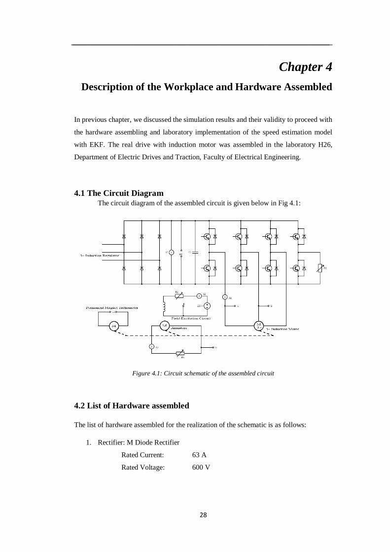
4.1 The Circuit Diagram The circuit diagram of the assembled circuit is given below in Fig 4.1:

Figure 4.1: Circuit schematic of the assembled circuit

4.2 List of Hardware assembled

The list of hardware assembled for the realization of the schematic is as follows:

1. Rectifier: M Diode Rectifier

Rated Current: 63 A

Rated Voltage: 600 V

_______________________________________________________________________

29

2. Current and Voltage Measurement interface for the DS1103:

Rated Current: 200A

Rated Voltage: 800V

In every LEM current sensor, there was five turns of the phase wire in

order to increase the measurement accuracy, so the maximum current for

each coil was 40A. Since the induction motor rated current is 2A only,

more turns could have been present in order to increase the accuracy more.

But because of the space limitation we could not accommodate more coil

turns to increase the accuracy of the sensor.

3. IGBT:

6 CM100DY-24NF IGBT [11] by Mitsubishi Electric used for motor

control, with 2 more used as a safety layers in case of overvoltage , with

a break resistor R1 rated at 420Ω.

4. DC-Link Capacitors:

Rated Voltage: 450 V

Rated Capacitance: 4700 µF

Two capacitors of the above rated parameters each, connected in series to

make capacitor bank for the DC-link.

5. Induction Motor:

Y-connnected

Rated Voltage: 380 V

Rated Current: 2 A

Rated Power: 750 W

Nominal speed: 1380 rpm

Power Factor (cosφ): 0.79

Frequency: 50 Hz

6. DC Motor:

Rated Power: 1.2 kW

Armature:

Rated Voltage: 400 V

Rated Current: 3.8 A

_______________________________________________________________________

30

Field Excitation Circuit:

Rated Voltage: 220 V

Rated Current: 0.6 A

Nominal Speed: 1650 rpm

7. Permanent Magnet Tachometer:

Tachometer aligned to the same shaft as the DC motor and Induction

motor. The tachometer is calibrated at 80V/1000 rpm

8. Resistors:

For overvoltage protection (R1): 1.2 A 420 Ω

For DC motor Field excitation (R2): 4 A 39 Ω

For DC Motor Armature Winding (R3): 0.63 A 200 Ω

(3 resistors used in series) 1.6 A 250 Ω

2.5A 105 Ω

9. DS1103 PPC Controller Board [12]:

The dSPACE board is used as a microcontroller along with its controller

UI desk. In the above circuit the measurements from the points U1, U2,

I1, I2, I3 and I4 are taken to process and compute the required

measurement quantities. U1 was used for the dc-link voltage for the

inverter calculations, U2 was used to get the measured speed of the motor,

I1 and I2 for the stator current measurements and I3 and I4 for the load

measurements.

10. Voltmeter:

One Voltmeter rated at 600V is used to check the DC-link voltage.

11. Ammeter:

Three Ammeters are used at: the Excitation winding of the DC motor,

Armature of the motor DC motor, and the input to one of the windings of

the Induction motor. There were used to ensure the currents do not exceed

the rated current while changing the load values for the experiment. DC

ammeters and AC millimeters were used accordingly in circuits.

_______________________________________________________________________

31

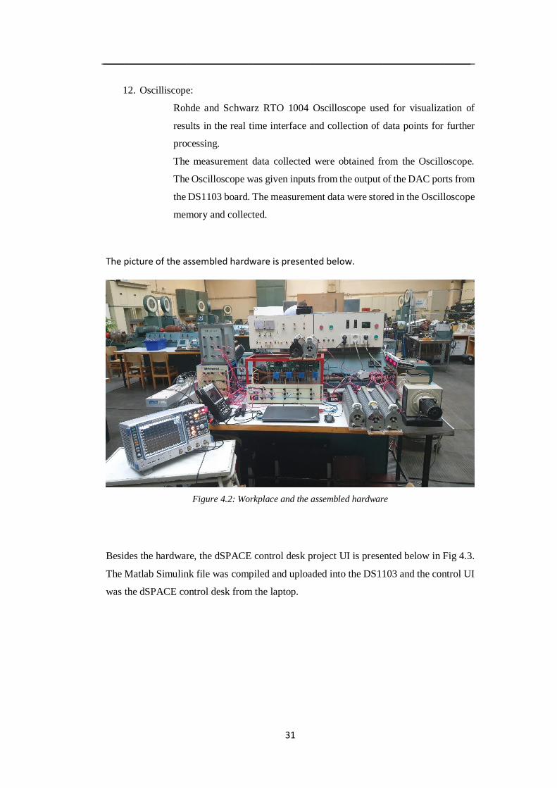
12. Oscilliscope:

Rohde and Schwarz RTO 1004 Oscilloscope used for visualization of

results in the real time interface and collection of data points for further

processing.

The measurement data collected were obtained from the Oscilloscope.

The Oscilloscope was given inputs from the output of the DAC ports from

the DS1103 board. The measurement data were stored in the Oscilloscope

memory and collected.

The picture of the assembled hardware is presented below.

Figure 4.2: Workplace and the assembled hardware

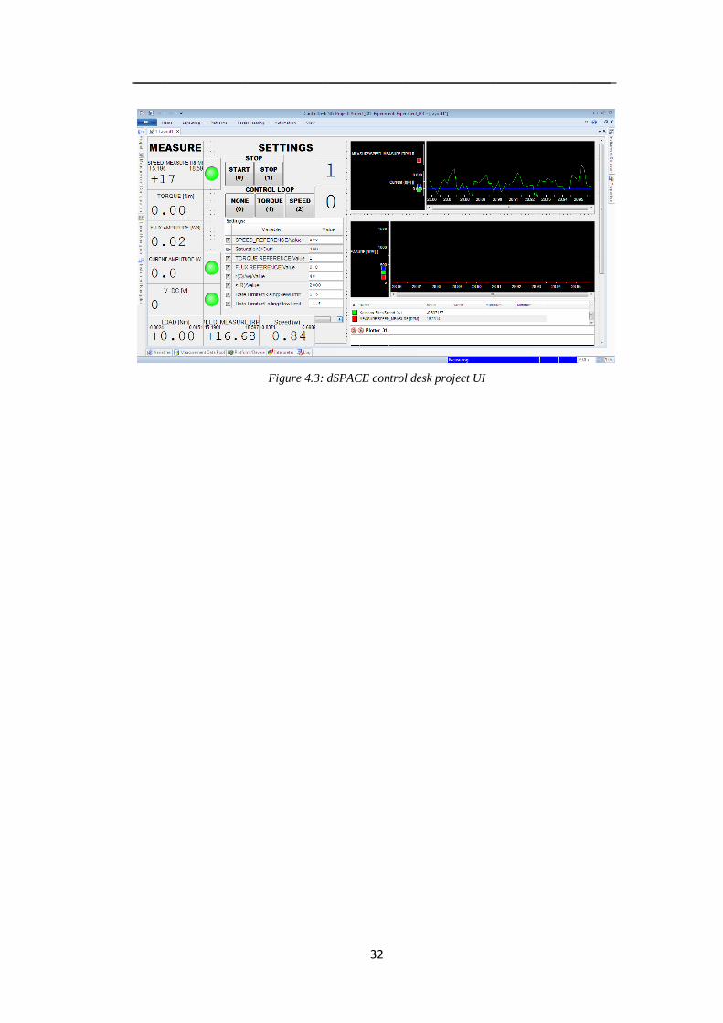
Besides the hardware, the dSPACE control desk project UI is presented below in Fig 4.3.

The Matlab Simulink file was compiled and uploaded into the DS1103 and the control UI

was the dSPACE control desk from the laptop.

_______________________________________________________________________

32

Figure 4.3: dSPACE control desk project UI

_______________________________________________________________________

33

Chapter 5

Experimental Results

After assembling the hardware, we experimented the various cases of the motor

operations that included the loaded and unloaded operations, changing the values of filter

noise covariance matrices Q and R and their effects on transient and steady-state

performances and tuning them based on the desired operation, low speed performance and

the performance under varying load.

Regarding the sampling time of the experimentation loops, all the experimentation

was done with a sampling time of 150µs. This is because we could not gain a better

sampling time in the experimentation due to the computational limitation of the hardware

used (DS1103) and computational requirements of the filter.

5.1 Steady State Operation of the Motor.

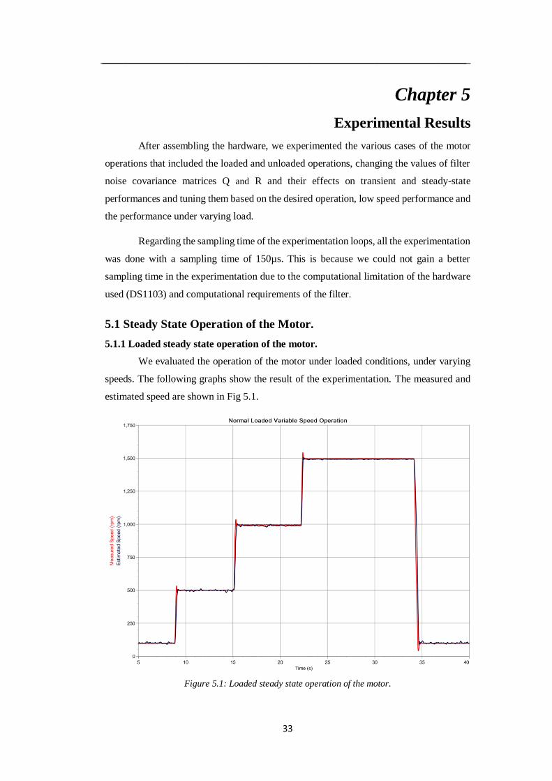
5.1.1 Loaded steady state operation of the motor.

We evaluated the operation of the motor under loaded conditions, under varying

speeds. The following graphs show the result of the experimentation. The measured and

estimated speed are shown in Fig 5.1.

Figure 5.1: Loaded steady state operation of the motor.

_______________________________________________________________________

34

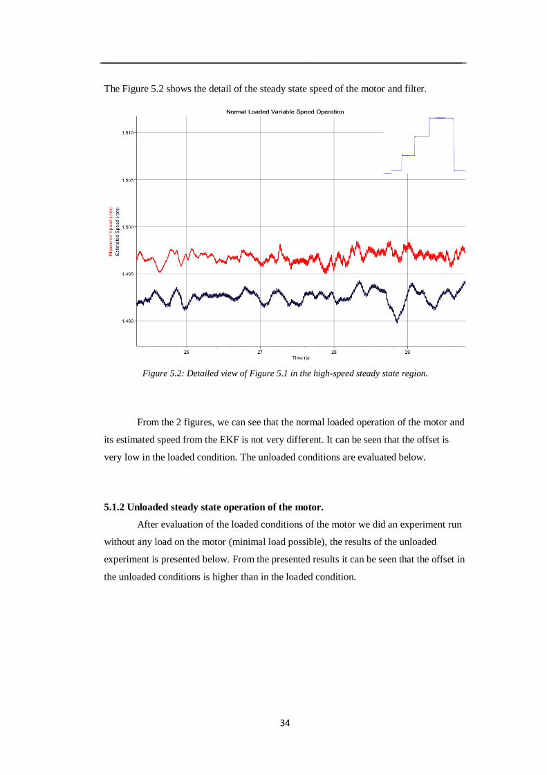
The Figure 5.2 shows the detail of the steady state speed of the motor and filter.

Figure 5.2: Detailed view of Figure 5.1 in the high-speed steady state region.

From the 2 figures, we can see that the normal loaded operation of the motor and

its estimated speed from the EKF is not very different. It can be seen that the offset is

very low in the loaded condition. The unloaded conditions are evaluated below.

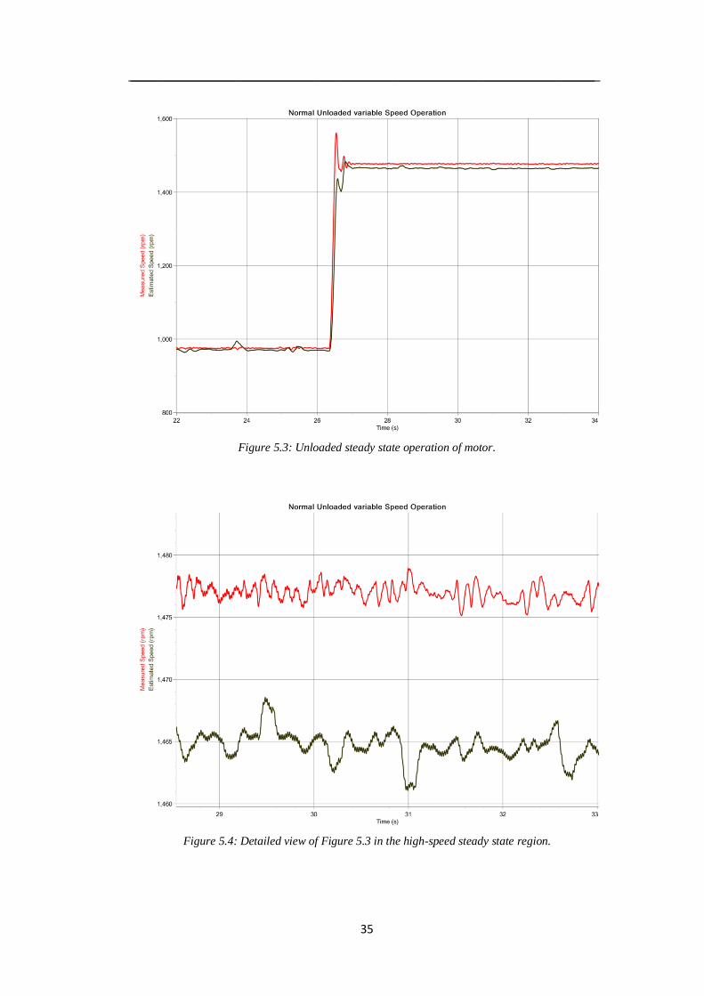
5.1.2 Unloaded steady state operation of the motor.

After evaluation of the loaded conditions of the motor we did an experiment run

without any load on the motor (minimal load possible), the results of the unloaded

experiment is presented below. From the presented results it can be seen that the offset in

the unloaded conditions is higher than in the loaded condition.

_______________________________________________________________________

35

Figure 5.3: Unloaded steady state operation of motor.

Figure 5.4: Detailed view of Figure 5.3 in the high-speed steady state region.

_______________________________________________________________________

36

5.1.3 Comparison of loaded and unloaded operation mode

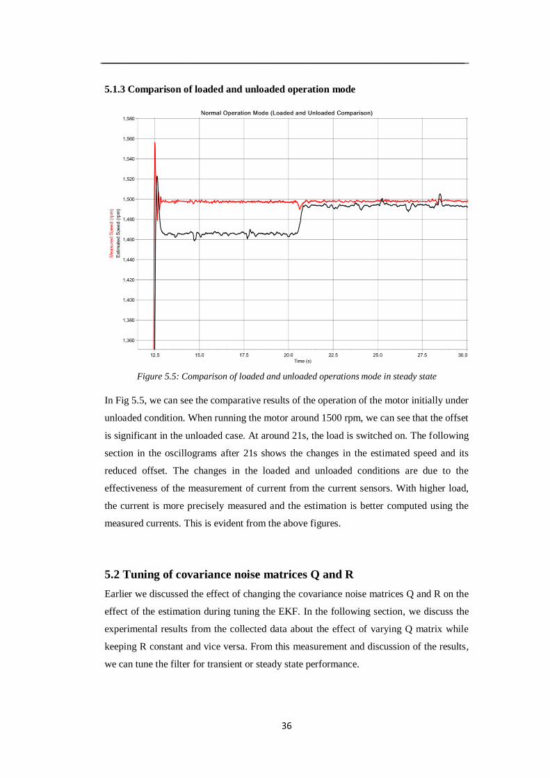
Figure 5.5: Comparison of loaded and unloaded operations mode in steady state

In Fig 5.5, we can see the comparative results of the operation of the motor initially under

unloaded condition. When running the motor around 1500 rpm, we can see that the offset

is significant in the unloaded case. At around 21s, the load is switched on. The following

section in the oscillograms after 21s shows the changes in the estimated speed and its

reduced offset. The changes in the loaded and unloaded conditions are due to the

effectiveness of the measurement of current from the current sensors. With higher load,

the current is more precisely measured and the estimation is better computed using the

measured currents. This is evident from the above figures.

5.2 Tuning of covariance noise matrices Q and R

Earlier we discussed the effect of changing the covariance noise matrices Q and R on the

effect of the estimation during tuning the EKF. In the following section, we discuss the

experimental results from the collected data about the effect of varying Q matrix while

keeping R constant and vice versa. From this measurement and discussion of the results,

we can tune the filter for transient or steady state performance.

_______________________________________________________________________

37

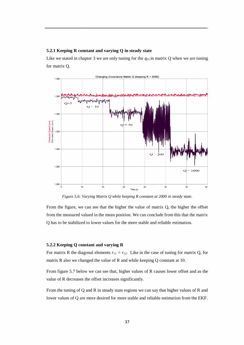
5.2.1 Keeping R constant and varying Q in steady state

Like we stated in chapter 3 we are only tuning for the q55 in matrix Q when we are tuning

for matrix Q.

Figure 5.6: Varying Matrix Q while keeping R constant at 2000 in steady state.

From the figure, we can see that the higher the value of matrix Q, the higher the offset

from the measured valued in the mean position. We can conclude from this that the matrix

Q has to be stabilized to lower values for the more stable and reliable estimation.

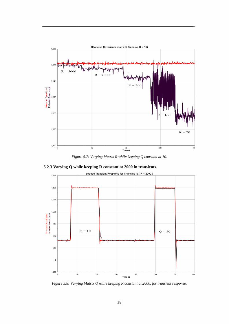
5.2.2 Keeping Q constant and varying R

For matrix R the diagonal elements r11 = r22. Like in the case of tuning for matrix Q, for

matrix R also we changed the value of R and while keeping Q constant at 10.

From figure 5.7 below we can see that, higher values of R causes lower offset and as the

value of R decreases the offset increases significantly.

From the tuning of Q and R in steady state regions we can say that higher values of R and

lower values of Q are more desired for more stable and reliable estimation from the EKF.

_______________________________________________________________________

38

Figure 5.7: Varying Matrix R while keeping Q constant at 10.

5.2.3 Varying Q while keeping R constant at 2000 in transients.

Figure 5.8: Varying Matrix Q while keeping R constant at 2000, for transient response.

_______________________________________________________________________

39

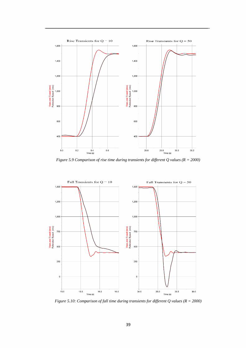
Figure 5.9 Comparison of rise time during transients for different Q values (R = 2000)

Figure 5.10: Comparison of fall time during transients for different Q values (R = 2000)

_______________________________________________________________________

40

In figure 5.8 we can see the transient responses for 2 different values of Q. Figure 5.9

shows the comparison of rising transient characteristics. From the figure, we can see that

the rise time for higher Q value is faster and the estimation is more accurate than for the

lower Q value. In figure 5.10, we can see the fall transient characteristics. Here in the case

of higher Q value, the transient has better estimation in the initial stage but as the final

value is reached the estimation has an overshoot peak, which is damped very quickly

though. However, in the case of the lower Q value, the fall time is much higher and the

deviation is higher in estimation as well.

From the above experimentation, we can say that the lower Q values are preferred in stable

states and moderate Q values are preferred for the faster transients. For a mixed operation,

the balance between lower offset and faster transient is chosen as per the necessities.

Because of this reasons for all the experimentation, for steady state Q = 10 and R = 2000

is taken, and for the transients, Q=50 and R =2000 is taken.

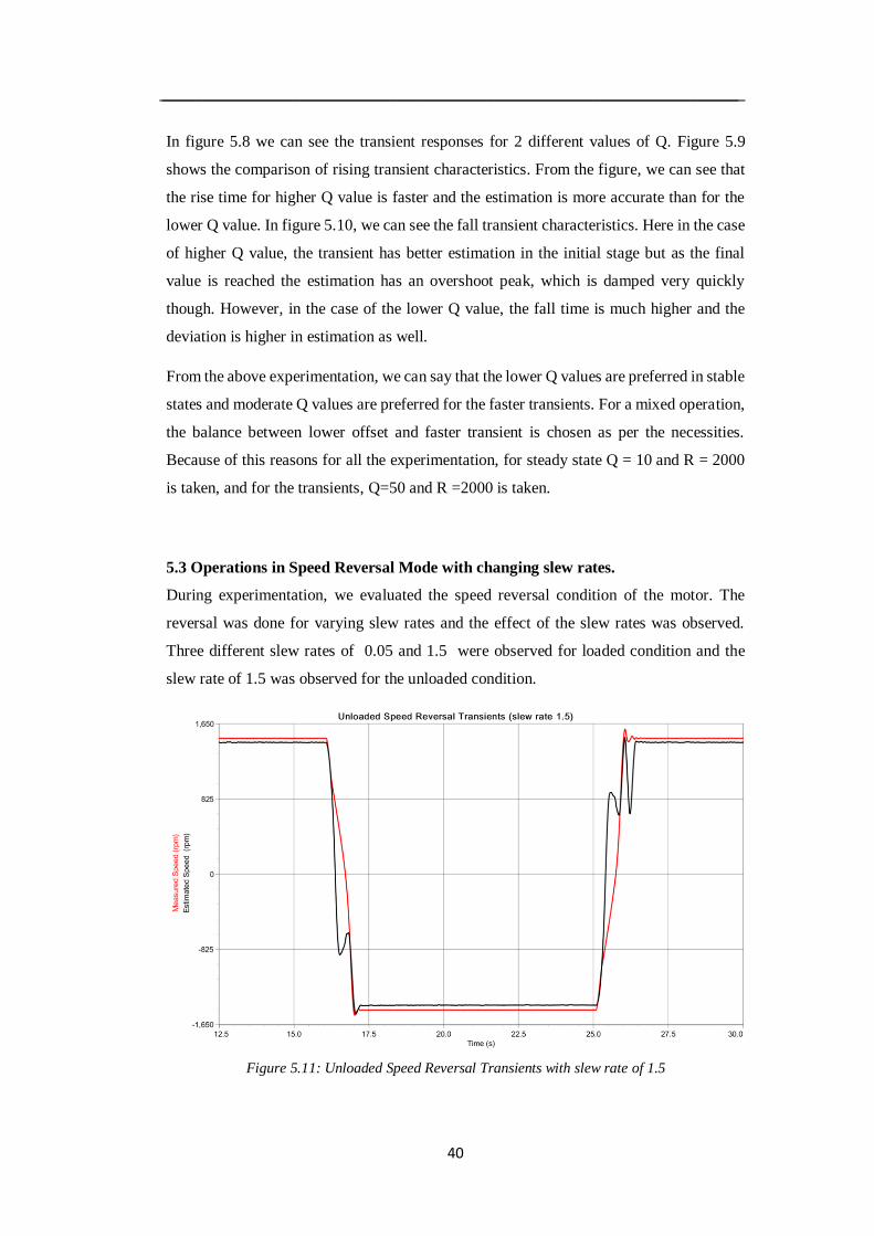
5.3 Operations in Speed Reversal Mode with changing slew rates.

During experimentation, we evaluated the speed reversal condition of the motor. The

reversal was done for varying slew rates and the effect of the slew rates was observed.

Three different slew rates of 0.05 and 1.5 were observed for loaded condition and the

slew rate of 1.5 was observed for the unloaded condition.

Figure 5.11: Unloaded Speed Reversal Transients with slew rate of 1.5

_______________________________________________________________________

41

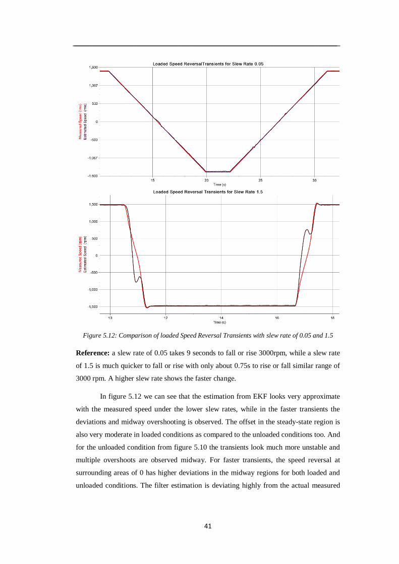
Figure 5.12: Comparison of loaded Speed Reversal Transients with slew rate of 0.05 and 1.5

Reference: a slew rate of 0.05 takes 9 seconds to fall or rise 3000rpm, while a slew rate

of 1.5 is much quicker to fall or rise with only about 0.75s to rise or fall similar range of

3000 rpm. A higher slew rate shows the faster change.

In figure 5.12 we can see that the estimation from EKF looks very approximate

with the measured speed under the lower slew rates, while in the faster transients the

deviations and midway overshooting is observed. The offset in the steady-state region is

also very moderate in loaded conditions as compared to the unloaded conditions too. And

for the unloaded condition from figure 5.10 the transients look much more unstable and

multiple overshoots are observed midway. For faster transients, the speed reversal at

surrounding areas of 0 has higher deviations in the midway regions for both loaded and

unloaded conditions. The filter estimation is deviating highly from the actual measured

_______________________________________________________________________

42

speed in those regions. But for the lower slew rates, the same problem is not observed as

seen in the above graphical results.

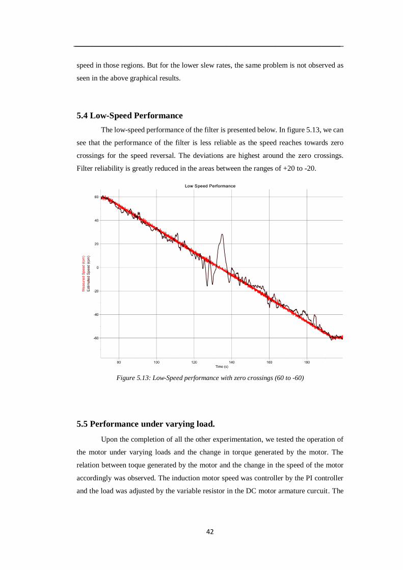
5.4 Low-Speed Performance

The low-speed performance of the filter is presented below. In figure 5.13, we can

see that the performance of the filter is less reliable as the speed reaches towards zero

crossings for the speed reversal. The deviations are highest around the zero crossings.

Filter reliability is greatly reduced in the areas between the ranges of +20 to -20.

Figure 5.13: Low-Speed performance with zero crossings (60 to -60)

5.5 Performance under varying load.

Upon the completion of all the other experimentation, we tested the operation of

the motor under varying loads and the change in torque generated by the motor. The

relation between toque generated by the motor and the change in the speed of the motor

accordingly was observed. The induction motor speed was controller by the PI controller

and the load was adjusted by the variable resistor in the DC motor armature curcuit. The

_______________________________________________________________________

43

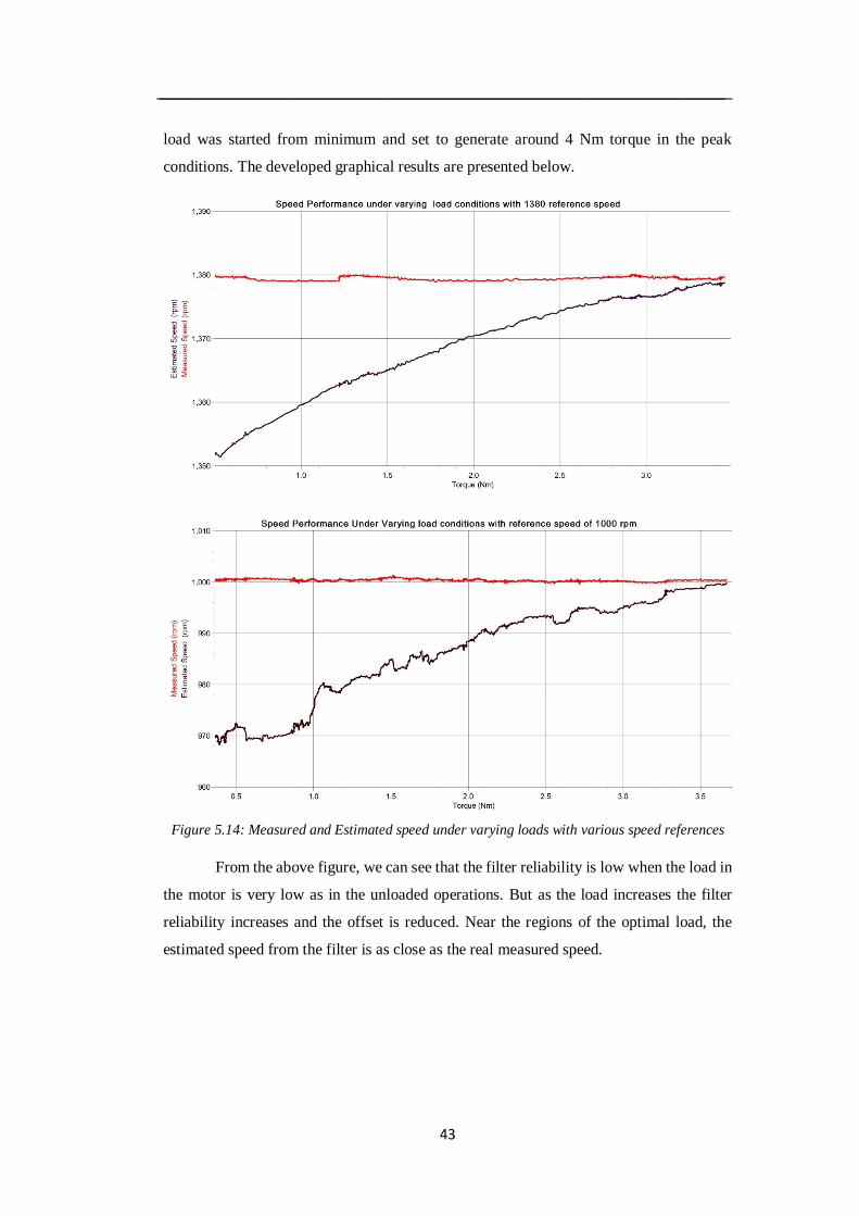
load was started from minimum and set to generate around 4 Nm torque in the peak

conditions. The developed graphical results are presented below.

Figure 5.14: Measured and Estimated speed under varying loads with various speed references

From the above figure, we can see that the filter reliability is low when the load in

the motor is very low as in the unloaded operations. But as the load increases the filter

reliability increases and the offset is reduced. Near the regions of the optimal load, the

estimated speed from the filter is as close as the real measured speed.

_______________________________________________________________________

44

Chapter 6

Conclusion

Motor control has been an essential part of the industrial sector. With the

automated controls, we are moving farther and distant from the manuals controls every

other day. The reliance on sensors has been decreasing and the automation towards

sensorless controls has been the new wave of control mechanisms. The elimination of

sensors makes the control strategy more economically viable. With the increasing

computational power of smaller ICs, the dependence on the algorithms for estimations of

speed with high reliability on the output has been a greater advantage for this control

sector. Going with the theories behind one of the estimation algorithms, in this thesis paper

we tested one of such algorithms: Extended Kalman Filter. An EKF was designed,

developed, and implemented with the hardware realization on a laboratory motor.

The results of the experiment were in accordance with the simulations. The

hardware implementation in this project paper gave the idea of the difficulties when

moving from simulation model to real hardware. One of such instances was the limitation

of the computation power of the signal processor used. While in simulations, the lower

sampling times were achieved with lower offsets, in the hardware scenarios, the sampling

times were limited to 150µs. This lead to the expectance of the offsets in the estimated

results from the EKF. While in some fronts the hardware developments with the real-time

interface were much easier to control than in simulations, like the tuning of the filter

covariance matrices and the assessment of the transient dynamic.

The results in this thesis show the effectiveness of the filter with low error

percentages under the right tuning of the filter covariance matrices. The results show that

tuning of covariance matrices in the filter plays a big role in the ultimate output of the filter

and its accuracy. As discussed prior, based on the suitability of the applications being

transient analysis on the motor or the steady-state responses of the motor the tuning should

be done accordingly. The results from chapter 5 show the differences in the tuning

parameters, and their necessity to be chosen appropriately.

With the right tuning parameters, the filter accuracy can be discussed from the

results very clearly. The loaded and unloaded operation of the motor shows the difference

in offsets, mainly due to the current sensitivity of the current sensors used. We can state

_______________________________________________________________________

45

from the loaded conditions that the filter behaves very accurate even under unloaded

conditions if more sensitive current measurement devices are taken into consideration.

Similar to the loaded and unloaded operations in steady-state conditions at normal speeds,

the performed tests show that the filter works properly in speed reversal conditions as well.

This is an important aspect in the case of bidirectional motors. The reliability of the filter

in both the direction of the rotation axis shows the filter versatility and accuracy.

For the low-speed regions, the reliability of the filter has been worse. There is a

room for improvement in the filter algorithm that can access these low-speed estimations

with very low-speed dynamics during speed reversals near zero crossings.

Besides the low speed and offset issues, other regions for decreased reliability in

the filter could be because of the system description not being 100% accurately described.

The parameters of the motor were measured in certain operation point (loaded motor) and

with some uncertainty. Moreover, the changes that occur with the temperate on resistances

and load magnetization curves of inductance is not taken into consideration. Also the

sampling time taken from the computational device is very long. And the measurement of

current was in the range of 40A accuracies while the motors nominal current was around

2A. The voltages were calculated from the DC link and transistor combination, so the other

nonlinearities in the model due to switching time delays and voltage drops of the inverter

are also not considered. In regards to these factors not being in consideration, the

estimation can be made better with the inclusion of these factors in future.

Overall the development and performance of the filter form this thesis

experimentation and simulation can be said to be accurate small deviations and offsets in

nominal steady states, while the room for improvement is always there. The tested results

for various operating conditions as discussed above serve as backing data for the

effectiveness of the filter developed.

Work for Future.

While the extent of this thesis was limited to the estimation for the speed of the

IM without any speed sensors, the work from this experiment can be carried further ahead

on the other control experiments. The estimated speed can be fed back as a closed loop

control for sensorless vector control of the IM. This regime of control is the new control

_______________________________________________________________________

46

strategy that is more economic with the employment of fewer sensors and is also

economically more suitable.

Further work can be done as discussed above on the better representation of the

model considering all the other factors stated above. Besides that the computational

requirements can also be reduced for faster sampling times with code optimization.

_______________________________________________________________________

47

Chapter 7

References

[1] F. Wang, Z. Zhang, X. Mei, J. Rodríguez, and R. Kennel, “Advanced control strategies of induction machine: Field oriented control, direct torque control and model predictive control,” Energies, vol. 11, no. 1, 2018.

[2] R. Gunabalan, V. Subbiah, and B. Reddy, “Sensorless control of induction motor with extended Kalman filter on TMS320F2812 processor,” Measurement, vol. 2, no. 5, pp. 14–19, 2009.

[3] T. RAMESH, A. K. PANDA, S. . KUMAR, and S. BONALA, “Sensorless control of

induction motor drives,” Proc. IEEE, vol. 90, no. 8, pp. 1359–1394, 2002.

[4] G. Welch, G. Bishop, “An Introduction to the Kalman Filter” , TR 95-041,

Department of Computer Science, University of North Carolina at Chapel Hill,

Chapel Hill-, NC-27599-3175, 24th July, 2006

[5] F. Orderud, “Comparison of kalman filter estimation approaches for state

space models with nonlinear measurements,” … Scand. Conf. Simul. …, vol.

194, no. 7491, pp. 157–162, 2005.

[6] M. Madhumita, “Study of Kalman, Extended Kalman and Unscented Kalman

Filter (an approach to design a power system harmonic estimator),” 2010.

[7] Y. Kim and H. Bang, “Introduction to Kalman Filter and Its Applications,” Introd.

Implementations Kalman Filter, no. September, 2018.

[8] M. I. Ribeiro, “Kalman and Extended Kalman Filters : Concept , Derivation and

Properties,” Inst. Syst. Robot. Lisboa Port., no. February, p. 42, 2004.

[9] M.-H. P. Young-Real Kim, Seung-Ki Sul, “Speed Sensorless Vector Control of IM

using EKF,” vol. 30, no. 5, pp. 1225–1233, 1994.

[10] P. Karlovsky and J. Lettl, “Induction motor drive direct torque control and

predictive torque control comparison based on switching pattern analysis,”

Energies, vol. 11, no. 7, 2018.

[11] Mitsubishi Electric, “CM100DY-24F”, pp. 1–5, 2009.

[12] dSPACE, “DS1103 PPC Controller Board”, pp. 1-8, 2008

_______________________________________________________________________

48

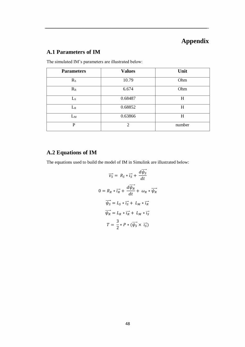
Appendix

A.1 Parameters of IM

The simulated IM’s parameters are illustrated below:

Parameters Values Unit

RS 10.79 Ohm

RR 6.674 Ohm

LS 0.68487 H

LR 0.68852 H

LM 0.63866 H

P 2 number

A.2 Equations of IM

The equations used to build the model of IM in Simulink are illustrated below:

𝑣𝑆 = 𝑅𝑆 ∗ 𝑖𝑆 + 𝑑𝜓𝑆

𝑑𝑡

0 = 𝑅𝑅 ∗ 𝑖𝑅 + 𝑑𝜓𝑅

𝑑𝑡+ 𝜔𝑅 ∗ 𝜓𝑅

𝜓𝑆 = 𝐿𝑆 ∗ 𝑖𝑆 + 𝐿𝑀 ∗ 𝑖𝑅

𝜓𝑅 = 𝐿𝑅 ∗ 𝑖𝑅 + 𝐿𝑀 ∗ 𝑖𝑆

𝑇 = 3

2∗ 𝑃 ∗ (𝜓𝑆

× 𝑖𝑆 )