Determination of Mandelbrot Set’s

Hyperbolic Component Centres

G. Álvarez, M. Romera, G. Pastor and F. Montoya

INSTITUTO DE FÍSICA APLICADA,

CONSEJO SUPERIOR DE INVESTIGACIONES CIENTÍFICAS

SERRANO 144, 28006 MADRID

E-mail: gonzalo@iec.csic.es

Abstract: In this work we present a very fast and parsimonious

method to calculate the centre coordinates of hyperbolic components in the

Mandelbrot set. The method we use constitutes an extension for the complex

domain of the one developed by Myrberg for the real map pxx −2֏ , in

which given the symbolic sequence of a superstable orbit, the parameter

value originating such superstable orbit is worked out. We show that when

dealing with complex domain sequences, some of the solutions obtained

correspond to the centres of the Mandelbrot set’s hyperbolic components,

while some others do not exist.

2

1. Introduction

According to Hao and Zheng [1], historically the symbolic dynamics appeared in

topological dynamical systems theory during the 30’s. Being the only rigorous way to

describe the chaotic movement in dynamical systems, its abstract mathematical form is

hard to understand and to apply to the study of concrete models. However, in the case of

unimodal maps, an applied symbolic dynamics was developed, constituting a valuable

tool. The most important study about symbolic dynamics belongs to Metropolis, Stein

and Stein [2] (MSS). In a previous work [3], we showed a sketch of the hyperbolic

components generation in one dimensional quadratic maps using symbolic dynamics

and the MSS algorithm.

Let us consider the real Mandelbrot map cxx nn +=+2

1 . To represent the dynamics of a

given orbit, we do not record the exact value of each iterate ix , but consider simply if it

falls to the left (L), to the right (R) or on the critical point (C). Thus, for instance, the

symbolic sequence of the period-2 superstable orbit is CLCLCL…. When restricted to a

single period, it is written simply as CL.

Myrberg [4] proposed a method which leads straightforward to the parameter value

when the corresponding symbolic sequence is known. To find for instance the

c-parameter value of the period-3 superstable orbit with symbolic sequence CLR, it is

enough to solve the equation ccc −+−−= , which can be easily accomplished

iterating (note that the solution is the fixed point of the map nnn ccc −+−−=+1 ).

In general, the c value of the real Mandelbrot map’s parameter originating a real

superstable orbit of a given symbolic sequence CLRXX…X (the first three letters are

3

always CLR for superstable orbits on the real axis) can be obtained by Myrberg’s

formula [4]:

ccccc −±±−±−+−−= ... , (1)

where the symbol ± stands for a + sign or a – sign according to the expression of the

orbit’s symbolic dynamics, assigning the + sign to the letter R and the – sign to the

letter L. The first sign before the square root is always –, and corresponds to the first L

in the orbit’s symbolic dynamics, whereas the second sign is always +, corresponding to

the first R (CLRXX…X).

This simple but efficient method put forward by Myrberg, and used later by Kaplan [5],

Zheng and Hao [6], Schroeder [7], and others, allows to obtain fast and parsimoniously

the parameter value of an orbit of any period n for the real Mandelbrot map. For

example, the parameter value c = –1.78187000761051…, corresponding to the period-

24 orbit of symbolic sequence LRLRRLRLCLR4

2222 , where

222242 LRLRLRLRLR = , can easily be found applying this method [8].

In this work we pretend to prove that this method also works for the complex plane

extension, i.e., it will be shown that when applying the method devised by Myrberg for

finding the parameter value originating orbits in the complex plane, the centres of the

hyperbolic components [9] of the Mandelbrot set are obtained.

2. Extension of Myrberg’s Method to the Complex Plane

Let us consider now the complex Mandelbrot map

czzpz ncn +==+2

1 )( , (2)

4

where C∈cz, . As is well known, the Mandelbrot set, M, can be defined as the set of

c-parameter values for which the orbit of the critical point, z0 = 0, remains bounded, i.e.,

it does not tend to infinity as n tends to infinity:

M = { ∞→/∈ )0(| ncpc C when ∞→n }, (3)

where )(zpnc represents the n-th iteration of function (2), dependant on the c-parameter.

The real solutions considered in the introduction correspond to the centres of cardioids

or disks (hyperbolic components) on the Mandelbrot set’s antenna (on the real axis), but

what happens when we obtain pairs of complex conjugate solutions after applying

Myrberg’s method to sequences of letters not corresponding to real orbits? Let us

consider, for example, the orbit of symbolic sequence CLL. In this case, we obtain two

complex conjugate solutions. When carefully examining these solutions, it is easy to

realise that they correspond to the centres of the two biggest disks attached to the main

cardioid of the Mandelbrot set (see Fig. 1). Therefore, solving Myrberg’s formula for

different combinations of signs (different symbolic sequences), we normally obtain

pairs of complex conjugate solutions which correspond to centres of cardioids or disks

on the set’s periphery, although in some cases we can not obtain a solution because

Myrberg’s formula does not converge.

In this context, and only as a very simple and useful operative tool, we shall develop an

informal way of assigning complex sequences using the location of the orbit relative to

the imaginary axis because it serves to our purpose of calculating the centres of the

hyperbolic components. Thus, we shall consider the symbolic sequence of a complex

superstable period-n orbit of the Mandelbrot set to be ��� 1

XX...XC−n

, where we assign the

5

letter L to the iterates falling to the left of the imaginary axis and the R, to the iterates

falling to the right. C represents the map’s critical point, z = 0 + 0i. It is important to

note that we are aware that sequences of complex numbers do not have a natural order

and thus we do not pretend a rigorous description of orbits nor an extension of the

kneading theory to the complex case (see the beautiful external rays theory by Douady

and Hubbard [10] or [11]), but a useful operative way of describing orbits in order to

find hyperbolic component centres, as will be seen later in this section. Another point to

notice is that with this notation there always exist two symmetric orbits with respect to

the real axis for each symbolic sequence, although it represents no inconvenience for

our goal. For example, the symbolic sequence of the superstable period-3 orbits

corresponding to the two disks tangent to the main cardioid of the Mandelbrot set (Fig.

1) is CLL for both disks. Hence, a single symbolic sequence gives rise to a pair of

complex conjugate centres. In Table 1 are listed the values of these disks’ centres, along

with the orbit followed by the critical point. Therefore, when talking about symbolic

sequences in the complex case, we always mean two symmetric complex orbits with

respect to the real axis.

By simple combinatory, the maximum possible number of symbolic sequences of

period n is 12 −n (for example, for n = 5, there exist 16 possible symbolic sequences),

although not all of them will exist, as will be seen next. Provided that now the first two

letters following to the C do not need to be L and R, respectively, as in the real case, all

the possible ± signs in Myrberg’s formula

nnnn cccc −±±−±−±=+ ...1 (4)

6

should be considered. We call Eq. (4) the Myrberg map. As shown in [12], the number

of period-n real orbits and the total number of period-n orbits in unimodal maps, both

real and complex, can be calculated from a formula devised by Weiss and Rogers [13]

and by Lutzky [14]. These results are summarised in Table 2, which we have worked

out until period 16. Rn is the number of real orbits, and Cn is the total number of orbits,

both real and complex. According to Table 2, for n = 5 there exist 15 superstable orbits,

from which 3 are real and consequently 12 must be complex (6 complex conjugated

solutions). This means that out of the 16 possible letter combinations to make up the

symbolic sequences, only 3 sequences correspond to real orbits (CLR3, CLR2L,

CLRL2), while 6 sequences correspond to 6 pairs of symmetrical orbits (CLRLR, CL4,

CL2RL, CL2R2, CR2LR, CR3L). The remaining other 7 sequences do not exist (CL3R,

CRL3, CRL2R, CRLRL, CRLR2, CR2L2, CR4).

A method to work out the Mandelbrot set’s hyperbolic component centre coordinates of

a given period, consists of calculating the c-values for which the origin (the map’s

critical point) belongs to the period-n cycles in question: from Eq. (2), the values of the

centres looked for, c , can be found as the zeroes of the polynomials

0)()0( 1 =≡ − cpp nc

nc . (5)

As easily observed, for high periods this method becomes highly costly, requiring a

long computing time as n increases. The simple algebraic method developed by

Stephenson [12, 15, 16] of constructing exact analytical solutions to the parts of the

boundaries of the Mandelbrot set in the form of polynomial maps of the unit circle,

becomes almost impracticable for periods 10≥n , because the size of the numerical

7

coefficients and the number of terms in the various polynomials soon become too large

to handle.

In this discouraging context, we show that the complex solutions obtained from Eq. (4),

when fed the symbolic sequences corresponding to superstable points in the interior of

whatever hyperbolic components, and considering that C∈c in Eq. (4), correspond to

the centres of those cardioids and disks, on the Mandelbrot set’s periphery. In this way,

the extension of Myrberg’s formula to the complex plane allows us to easily find the

centres of the hyperbolic components of the Mandelbrot set.

Thus, when applying Myrberg’s method with C∈c to a given sequence, which we do

not know in advance whether it exists or not, one of three cases takes place:

a) The method converges to a real solution: this means that the orbit with such symbolic

sequence exists and is real. The value to which it converged is the centre of the disk or

cardioid centred at the Mandelbrot set’s antenna.

b) The method converges to a complex solution: this means that we have found one of

the two complex conjugated centres, and therefore there are two complex symmetric

orbits with such symbolic sequence.

c) The method does not converge to a value, real nor complex: in this case, we do not

know if this is due to a non-existent orbit, or to the failure of the method to converge. In

the former situation, we know of no method yet that can tell whether a given complex

symbolic sequence exists or not. In next section we shall see how to overcome the

difficulty of a non-converging but existing sequence.

8

3. Exceptional Points

In those cases when Myrberg’s method does not converge to a solution, we found a way

to transform the iterative Eq. (4) into an alternative one which does converge. For

example, for the period-5 complex symbolic sequence CR3L, corresponding to a disk

centre on the periphery of the Mandelbrot set, the dynamical system:

nnnnnn cccccfc −−−+−+−+==+ )(1 (6)

does not converge to the value looked for, ic ...3349323056.0...3795135881.0 ±= , i.e.,

c is an unstable fixed point of the map (6). As it is well known, the stability of a fixed

point is determined by its multiplier, cλ , defined as the absolute value of the derivative

of the map’s function evaluated at that fixed point, c .

In system (6), the multiplier, ...1.15670052=cλ , is greater than unity if evaluated at the

point c , corresponding to the disk’s centre. Therefore, for this map, c represents a

repelling fixed point. The way to solve this difficulty consists of studying an equivalent

dynamical system that does present an attracting fixed point at c . Squaring both

members in system (6):

ccccc −−−+−+−=2

and reordering:

ccccc −−−+−+=+ )1(

we obtain the new dynamical system

1)(1 +

−−−+−+==+

n

nnnnn

c

ccccgc

9

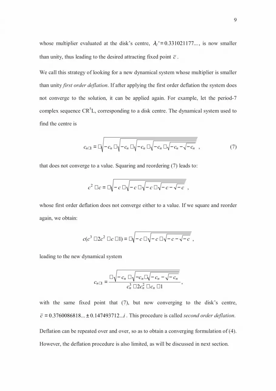
whose multiplier evaluated at the disk’s centre, ....3310211770'=cλ , is now smaller

than unity, thus leading to the desired attracting fixed point c .

We call this strategy of looking for a new dynamical system whose multiplier is smaller

than unity first order deflation. If after applying the first order deflation the system does

not converge to the solution, it can be applied again. For example, let the period-7

complex sequence CR5L, corresponding to a disk centre. The dynamical system used to

find the centre is

nnnnnnn ccccccc −−−+−+−+−+−+=+1 , (7)

that does not converge to a value. Squaring and reordering (7) leads to:

ccccccc −−−+−+−+−+=+2 ,

whose first order deflation does not converge either to a value. If we square and reorder

again, we obtain:

cccccccc −−−+−+−+=+++ )12( 23 ,

leading to the new dynamical system

12 231+++

−−−+−+−+=+

nnn

nnnn

nccc

ccccc ,

with the same fixed point that (7), but now converging to the disk’s centre,

ic ...147493712.0...3760086818.0 ±= . This procedure is called second order deflation.

Deflation can be repeated over and over, so as to obtain a converging formulation of (4).

However, the deflation procedure is also limited, as will be discussed in next section.

10

4. Limitations of the deflation method

It was shown how the method devised by Myrberg can be used not only for real values

of the map’s parameter, but for complex values as well. In the latter situation, in some

cases when the dynamical system (4) does not converge to a value, it must be

transformed into another one that does converge. This method, although working well

in most cases, does not always work. Thus, for period n = 7 (with 27 complex conjugate

solutions and 9 real solutions), it was not found an equivalent formulation of dynamical

system (4) converging for the symbolic sequence CRL2RL2, although the method works

correctly for the rest of sequences. For n = 8 (with 52 complex conjugate solutions and

16 real solutions), the method does not converge when trying to obtain 7 centres,

although it succeeds in finding the remaining 61 centres. The finding of alternative

ways of formulating the dynamical system (4), so that it does converge in all cases,

remains an open problem.

As a consequence, we deal with a method that, even though not infallible in all complex

cases, constitutes a valuable helping tool when working with high periods. Up to now,

no other method is known to algebraically find the hyperbolic components’ centres,

other than the resolution of Eq. (5) for C∈c or Stephenson’s method [12, 15, 16].

Unfortunately, for a relatively small period, such as n = 20, we find that the grade of

Eq. (5) is 524,288. To illustrate the problem’s complexity, in Fig. 2 the polynomial

corresponding to Eq. (5) has been plotted. As can be appreciated, the number of real

solutions (zero-crossings) is huge, exactly 26,214, whereas the total number of complex

conjugated solutions is 248,778. Even in the case that all solutions could be found, each

of them should be checked until the c-value corresponding to the given symbolic

11

sequence is found. Myrberg’s method, however, offers the possibility of finding the

solution fast and parsimoniously.

Let us see it with some examples. Firstly, given the period-20 symbolic sequence

CL4RL9RL4, when applying Myrberg’s formula, we reach easily to the solution

ic ...4.6121975420...9.5403140230 ±−= , that corresponds to a cardioid centre on

the periphery of the set.

Secondly, for the period-20 symbolic sequence CL2R2L2RL3RL3R2L2R, we obtain

directly the solution ic ...01.04170648...1680237817.0 ±−= , corresponding to

another cardioid centre as well.

Thirdly, for the period-20 symbolic sequence CLRL4RL4RL2RLRL2, we also obtain

directly the solution ic 760....00216360701...1.62427442 ±−= , corresponding to a

disk centre.

However, Myrberg’s method does not converge when trying the period-20 symbolic

sequence CR2L2R2LR3LR3L2R2L. But when applying the first order deflation, then the

solution ic 2....58936196107....3634622750 ±= is fast reached, that corresponds to a

cardioid centre.

As a last example, let us consider the period-30 symbolic sequence CL4RL14RL9. If the

polynomial resolution method is used, we find that the grade of Eq. (5) for n = 30

becomes 536,870,912, absolutely intractable. Likewise, it would be very costly to

explore each of the solutions to check which of the symbolic sequences they originate

coincides with the given one. On the contrary, if that sequence is tried with Myrberg’s

method, the solution ic 5....62730749509....5513177370 ±−= , that corresponds to a

disk centre, is reached without problems.

12

The overall performance of the extension of Myrberg’s method is summed up in Table

3 as the rate of convergence when searching for the centres (superstable points). The

number of symbolic sequences is calculated as nnnR

RC +−2

. It has to be noted that this

number is not simply Cn, since in the case of complex orbits there are always two orbits

with the same symbolic sequence.

5. Review of Results

In Table 4 we present the results obtained when the Myrberg method was applied

through period-7 symbolic sequences. The asterisks in the “Symbolic Sequence”

column inform of the order of deflation when applied: one * means first order deflation,

two *’s mean second order deflation. The plots in the “Basin of attraction of the

Myrberg map” column correspond to a graphical representation of the convergence of

the Myrberg’s formula. Initial points converging in the side-4 square centred at (0, 0) to

the centre of the superstable orbit are depicted in black. When the formula converges for

any point in the interior of the side-4 square, then the word “converges” appears.

6. Conclusions

We used and extended Myrberg’s method to find the c-parameter value of superstable

complex orbits, when only the symbolic sequence is known. Although the method

presented in this paper does not converge in all complex cases, it is the only

computationally reasonable alternative known to tackle the calculation of centres

corresponding to hyperbolic components from a given symbolic sequence.

13

Acknowledgements

This research was supported by CICYT, Spain, under grant no. TIC95-0080, and by

Comunidad de Madrid, Beca de Formación de Personal Investigador.

14

References

1. B.-L. Hao and W.-M. Zheng, “Symbolic Dynamics of Unimodal Maps Revisited”,

Int. J. Mod. Physics B, 3(2), 235-246 (1989).

2. N. Metropolis, M. L. Stein, and P. R. Stein, “On Finite Sets for Transformations

on the Unit Interval”, J. Combinatorial Theory, 15(1), 25-44 (1973).

3. G. Pastor, M. Romera and F. Montoya, Chaos, Solitons and Fractals, 7(4), 565-

584 (1996).

4. P. J. Myrberg, “Iteration der Reellen Polynome Zweiten Grades III”, An. Ac. Sci.

Fen., Series A, I. Mathematica, 336/3 (1963).

5. H. Kaplan, “New Method for Calculating Stable and Unstable Periodic Orbits of

One-dimensional Maps”, Physics Letters, 97(9), 365-367 (1983).

6. W.-M. Zheng, and B.-H. Hao, “Applied Symbolic Dynamics”, in Experimental

Study and Characterization of Chaos, ed. B.-L. Hao (World Scientific,

Singapore), (1990).

7. M. Schroeder, Fractals, Chaos, Power Laws (W. H. Freeman and Company, New

York) 263–299 (1991).

8. G. Pastor, M. Romera and F. Montoya, “Harmonic structure of one-dimensional

quadratic maps”, Physical Review E, 56(2), 1476-1483 (1997).

9. B. Branner, “The Mandelbrot Set”, Proceedings of Symposia in Applied

Mathematics, American Mathematical Society, 39, 75-105 (1989).

10. A. Douady and J. H. Hubbard, “Itération des polynômes quadratiques

complexes”, C. R. Acad. Sc. Paris, Série I Math., 294(3), 123-126 (1982).

15

11. J. H. Hubbard and D. Schleicher, “The Spider Algorithm”, Proceedings of

Symposia in Applied Mathematics, 49, 155-180 (1994).

12. J. Stephenson, “Formulae for cycles in the Mandelbrot set”, Physica A, 177, 416-

420 (1991).

13. A. Weiss and T. D. Rogers, Can. Math. Soc. Conf. Proc. 8 (Am. Math. Soc.,

Providence), p. 703 (1987).

14. M. Lutzky, “Counting Stable Cycles in Unimodal Iterations”, Physics Letters A,

131(4), 5 (1988).

15. J. Stephenson, “Formulae for cycles in the Mandelbrot set II”, Physica A, 190,

104-116 (1992).

16. J. Stephenson, “Formulae for cycles in the Mandelbrot set III”, Physica A, 190,

117-129 (1992).

16

Table 1. Superstable orbits corresponding to the complex symbolic sequence CLL.

Table 2. Number of real orbits, Rn, and total number of orbits (both real and complex),

Cn, depending on the period n.

Table 3. Performance of complex Myrberg’s method.

Table 4. Results of the application of complex Myrberg’s method through period-7

symbolic sequences. * indicates first order deflation. ** indicates second order

deflation.

Figure 1. Mandelbrot set representation, with the disks of complex symbolic sequence

CLL whose centres are at c = –0.1225611669…±0.7448617667…i.

Figure 2. Real Mandelbrot map. Critical polynomial for n = 20.

17

G. Álvarez, M. Romera, G. Pastor and F. Montoya

c –0.1225611669…+0.7448617667…i –0.1225611669…–0.7448617667…i

z0 0+0i 0+0i

z1 –0.1225611669…+0.7448617667…i –0.1225611669…–0.7448617667…i

z2 –0.66235897876…+0.562279512088…i –0.66235897876…–0.562279512088…i

Table 1

18

G. Álvarez, M. Romera, G. Pastor and F. Montoya

Table 2

n 2 3 4 5 6 7 8 9 10 11 12 13 14 15 16

Cn 1 3 6 15 27 63 120 252 495 1023 2010 4095 8127 16365 32640

Rn 1 1 2 3 5 9 16 28 51 93 170 315 585 1091 2048

19

G. Álvarez, M. Romera, G. Pastor and F. Montoya

Period # of symbolic sequences

# of sequences solved

Rate of convergence

2 1 1 1.00 3 2 2 1.00 4 4 4 1.00 5 9 9 1.00 6 16 16 1.00 7 36 35 0.97 8 68 61 0.90 9 140 123 0.88 10 273 239 0.88 11 558 482 0.86 12 1090 941 0.86 13 2205 1873 0.85 14 4356 3674 0.84 15 8728 7262 0.83 16 17344 14176 0.82

Table 3

20

G. Álvarez, M. Romera, G. Pastor and F. Montoya

Symbolic

Sequence

Centre

Coordinates

Basin of

attraction

C 0.0 converges

CL –1.0 converges CLR –1.75487766 converges CLL –0.12256116 ± 0.74486176i converges CLRR –1.94079980 converges CLRL –1.31070264 converges CLLR –0.15652016 ± 1.03224719i converges

CRRL 0.28227139 ± 0.53006061i

CLRRR –1.98542425 converges CLRRL –1.86078252 converges CLRLR –1.25636793 ± 0.38032096i converges CLRLL –1.62541372 converges CLLRR –0.19804209 ± 1.10026953i converges CLLRL –0.04421235 ± 0.98658097i converges CLLLL –0.50434017 ± 0.56276576i converges

CRRLR 0.35925922 ± 0.64251373i

CRRRL* 0.37951358 ± 0.33493230i

CLRRRR –1.99637613 converges CLRRRL –1.96677321 converges CLRRLR –1.77289290 converges CLRRLL –1.90728009 converges CLRLRR –1.28408492 ± 0.42726889i converges

CLRLRL –1.13800066 ± 0.24033240i

CLRLLL –1.47601464 converges CLLRRR –0.21752674 ± 1.11445426i converges CLLRRL –0.16359826 ± 1.09778064i converges CLLRLR –0.01557038 ± 1.02049736i converges CLLRLL –0.11341865 ± 0.86056947i converges CLLLLR –0.59689164 ± 0.66298074i converges

CRRLLL 0.39653457 ± 0.60418181i

CRRRLR* 0.44332563 ± 0.37296241i

CRRRRL* 0.38900684 ± 0.21585065i

CRRLRR* 0.35989273 ± 0.68476202i

Symbolic

Sequence

Centre

Coordinates

Basin of

attraction

CLRRRRR –1.99909568 converges CLRRRRL –1.99181417 converges CLRRRLR –1.95370589 converges CLRRRLL –1.97717958 converges CLRRLRR –1.76926167 ± 0.05691950i converges CLRRLRL –1.83231520 converges CLRRLLR –1.92714770 converges CLRRLLL –1.88480357 converges CLRLRRR –1.29255806 ± 0.43819881i converges CLRLRRL –1.26228728 ± 0.40810432i converges CLRLRLL –1.25273588 ± 0.34247064i converges CLRLLRL –1.67406609 converges CLRLLLR –1.40844648 ± 0.13617199i converges CLRLLLL –1.57488914 converges CLLRRRR –0.22491595 ± 1.11626015i converges CLLRRRL –0.20728383 ± 1.11748077i converges CLLRRLR –0.15751605 ± 1.10900651i converges CLLRRLL –0.17457822 ± 1.07142767i converges CLLRLRR –0.01423348 ± 1.03291477i converges

CLLRLRL –0.00693568 ± 1.00360386i

CLLRLLR –0.27210246 ± 0.84236469i converges CLLRLLL –0.12749997 ± 0.98746090i converges CLLLRLR –1.02819385 ± 0.36137651i converges CLLLLRR –0.62353248 ± 0.68106441i converges CLLLLRL –0.53082780 ± 0.66828872i converges CLLLLLL –0.62243629 ± 0.42487843i converges CRRRRRL** 0.37600868 ± 0.14474937i converges CRRRRLR* 0.43237619 ± 0.22675990i converges

CRRRLRR* 0.45277450 ± 0.39617012i

CRRRLLL* 0.45682328 ± 0.34775870i

CRRLRLL* 0.37689324 ± 0.67856869i

CRRLLRL 0.38653917 ± 0.56932471i converges

CRRLLLR 0.41291602 ± 0.61480676i

CRLLRRR* 0.35248253 ± 0.69833723i

CRLLRLL* 0.12119278 ± 0.61061169i

CRLLLLR* 0.01489546 ± 0.84814876i converges

Table 4

21

G. Álvarez, M. Romera, G. Pastor and F. Montoya

Figure 1

22

G. Álvarez, M. Romera, G. Pastor and F. Montoya

Figure 2