arX

iv:0

904.

2465

v10

[co

nd-m

at.s

tat-

mec

h] 9

Feb

201

0

Detrended fluctuation analysis of the magnetic and electric field variations that

precede rupture

P. A. Varotsos,1, ∗ N. V. Sarlis,1 and E. S. Skordas1

1Solid State Section and Solid Earth Physics Institute, Physics Department,

University of Athens, Panepistimiopolis, Zografos 157 84, Athens, Greece

Magnetic field variations are detected before rupture in the form of ‘spikes’ of alternating sign.The distinction of these ‘spikes’ from random noise is of major practical importance, since it is easierto conduct magnetic field measurements than electric field ones. Applying detrended fluctuationanalysis (DFA), these ‘spikes’ look to be random at short time-lags. On the other hand, long rangecorrelations prevail at time-lags larger than the average time interval between consecutive ‘spikes’with a scaling exponent α around 0.9. In addition, DFA is applied to recent preseismic electric fieldvariations of long duration (several hours to a couple of days) and reveals a scale invariant featurewith an exponent α ≈ 1 over all scales available (around five orders of magnitude).

Keywords: detrended fluctuation analysis, complex systems, scale invariance

PACS numbers:

Many physical and biological complex systemsexhibit scale-invariant features characterized bylong-range power-law correlations, which are of-ten difficult to quantify due to the presence of er-ratic fluctuations, heterogeneity and nonstation-arity embedded in the emitted signals. Here, wefocus on different types of nonstationarities suchas random spikes and pseudo-sinusoidal trends,that may affect the long-range correlation prop-erties of signals that precede rupture. Since thesenonstationarities may either be epiphenomena ofexternal conditions or may arise from the intrinsicdynamics of the system, it is crucial to distinguishtheir origin. This is attempted in the present pa-per for both the magnetic and the electric fieldvariations that appear before rupture by employ-ing the detrended fluctuation analysis (DFA) asa scaling method to quantify long-range temporalcorrelations. In particular, for the magnetic fieldvariations which have usually the form of ‘spikes’of alternating sign, we find that at short timescales they look to be random (thus may thenbe confused with random noise), but at largerscales long-range correlations prevail. As for theelectric field variations, that are usually superim-posed on a pseudo-sinusoidal background, uponusing the longest time series available to date (i.e.,with duration up to a couple of days), a scale-invariant feature over five orders of magnitudeemerges with an exponent close to unity.

I. INTRODUCTION

The detrended fluctuation analysis1–9 (DFA) is anovel method that has been developed to address theproblem of accurately quantifying long range corre-lations in non-stationary fluctuating signals. It hasbeen already applied to a multitude of cases includingDNA10–13, human motor activity14 and gait15,16, car-

diac dynamics17–20, meteorology21,22, climate tempera-ture fluctuations23. Traditional methods such as powerspectrum and autocorrelation analysis24 are not suitablefor non-stationary signals5,9.DFA is, in short, a modified root-mean-square (rms)

analysis of a random walk and consists of the followingsteps: Starting with a signal u(i), where i = 1, 2, . . . , N ,and N is the length of the signal, the first step is tointegrate u(i) and obtain

y(i) =i

∑

j=1

[u(j)− u] (1)

where u stands for the mean

u =1

N

N∑

j=1

u(j). (2)

We then divide the profile y(i) into boxes of equal lengthn. In each box, we fit y(i) using a polynomial functionyn(i) which represents the local trend in that box. (Ifa different order l of polynomial fit is used, we have adifferent order DFA-l, for example DFA-1 if l=1, DFA-2 if l=2, etc.) Next, the profile y(i) is detrended bysubstracting the local trend yn(i) in each box of lengthn:

Yn(i) = y(i)− yn(i). (3)

Finally, the rms fluctuation for the integrated and de-trended signal is calculated

F (n) ≡

√

√

√

√

1

N

N∑

i=1

[Yn(i)]2. (4)

The behavior of F (n) over a broad number of scales isobtained by repeating the aforementioned calculation ofF (n) for varied box length n. For scale invariant signals,we find:

F (n) ∝ nα (5)

2

where α is the scaling exponent. If α = 0.5, the signal isuncorrelated (white noise), while if α > 0.5 the signal iscorrelated.By employing the DFA method it was found25,26 that

long-range correlations exist in the original time-seriesof the so called seismic electric signals (SES) activities.These are low frequency (. 1Hz) electric signals preced-ing earthquakes27–32, the generation of which could beunderstood in the following context. A change of pres-sure affects the thermodynamic parameters for the for-mation, migration or activation, in general, of defects insolids33. In an ionic solid doped with aliovalent impuri-ties a number of extrinsic defects is produced,34,35 due tocharge compensation, a portion of which is attracted bynearby aliovalent impurities, thus forming electric dipolesthat can change their orientation in space through a de-fect motion36,37. Hence, pressure variations may affectthe thermodynamic parameters of this motion, thus re-sulting in a decrease or increase38 of the relaxation timeof these dipoles, i.e., their (re)orientation is taking placefaster or slower when an external electric field is applied.When the pressure, or the stress in general, reaches acritical value39 a cooperative orientation of these electricdipoles occurs, which results in the emission of a transientelectric signal. This may happen in the focal region ofa (future) earthquake since it is generally accepted thatthe stress gradually changes there before rupture.It has been shown40,41 that SES activities are better

distinguished from electric signals emitted from man-made sources, if DFA is applied to a signal after ithas been analyzed in a newly introduced time domain,termed natural time χ. In a time series comprising Nevents, the natural time χk = k/N serves as an index25

for the occurrence of the k-th event. The evolution ofthe pair (χk, Qk) is studied25,31,40–44, where Qk denotesa quantity proportional to the energy released in the k-thevent. For dichotomous signals, which is frequently thecase of SES activities, the quantity Qk stands for the du-ration of the k-th pulse. The normalized power spectrumΠ(ω) ≡ |Φ(ω)|2 was introduced, where

Φ(ω) =

N∑

k=1

pk exp

(

iωk

N

)

(6)

and pk = Qk/∑N

n=1 Qn, ω = 2πφ; φ stands for the natu-ral frequency. In natural time analysis, the properties ofΠ(ω) or Π(φ) are studied for natural frequencies φ lessthan 0.5, since in this range of φ, Π(ω) or Π(φ) reduces toa characteristic function for the probability distributionpk in the context of probability theory. When the systementers the critical stage, the following relation holds25,31:

Π(ω) =18

5ω2−

6 cosω

5ω2−

12 sinω

5ω3. (7)

For ω → 0, Eq.(7) leads to25

Π(ω) ≈ 1− 0.07ω2

which reflects31 that the variance of χ is given by

κ1 = 〈χ2〉 − 〈χ〉2 = 0.07,

where 〈f(χ)〉 =∑N

k=1 pkf(χk). The entropy S in thenatural time-domain is defined as41

S ≡ 〈χ lnχ〉 − 〈χ〉 ln〈χ〉,

which depends on the sequential order of events42. Itexhibits43 concavity, positivity, Lesche45,46 stability, andfor SES activities (critical dynamics) its value is smaller41

than the value Su(= ln 2/2−1/4 ≈ 0.0966) of a “uniform”(u) distribution (as defined in Refs.40–42, e.g. when allpk are equal or Qk are positive independent and identi-cally distributed random variables of finite variance. Inthis case, κ1 and S are designated κu(= 1/12) and Su,respectively.). Thus, S < Su. The same holds for thevalue of the entropy obtained43,44 upon considering thetime reversal T , i.e., T pk = pN−k+1, which is labelled byS−. In summary, the SES activities, in contrast to thesignals produced by man-made electrical sources, whenanalyzed in natural time exhibit infinitely ranged tempo-ral correlations40,41 and obey the conditions44:

κ1 = 0.07 (8)

and

S, S− < Su. (9)

For major earthquakes, i.e., with magnitude Mw6.5 orlarger, SES activities are accompanied47 by detectablevariations of the magnetic field B48. These variations,which are usually measured by coil magnetometers (seebelow), have the form of ‘spikes’ of alternating sign. It istherefore of interest to investigate whether these ‘spikes’exhibit long range temporal correlations. This investiga-tion, which is of major importance since only magneticfield data are usually available in most countries28,49,50

(since it is easier to conduct magnetic field measurementsthan electric field ones), is made here in Section II.In the up to date applications of DFA, long-range cor-

relations have been revealed in SES activities of durationup to a few hours25,26,40,41. During the last few years,however, experimental results related to some SES ac-tivities of appreciably longer duration, i.e., from severalhours to a couple of days, have been collected. Thesedata now enable the investigation of scaling in a widerrange of scales than hitherto known. This provides anadditional scope of the present paper and is carried outin Section III. A discussion of the results concerning themagnetic and electric data follows in Section IV. Finally,our conclusions are presented in Section V.

II. MAGNETIC FIELD VARIATIONS

PRECEDING RUPTURE

The measurements have been carried out by threeDANSK coil magnetometers (DMM) oriented along the

3

three axes: EW, NS and vertical. Details on the calibra-tion of these magnetometers can be found in the Supple-mentary Information of Ref.47. In particular, this cali-bration showed that for periods larger than around half asecond, the magnetometers measure51 the time derivativedB/dt of the magnetic field and their output is ‘neutral-ized’ approximately 200ms after the ‘arrival’ of a Heavi-side unit step magnetic variation. It alternatively meansthat a signal recorded by these magnetometers shouldcorrespond to a magnetic variation that has ‘arrived’ atthe sensor less than 200ms before the recording. Thedata were collected by a Campbell 21X datalogger withsampling frequency fexp = 1sample/s.

Figure 1(a) provides an example of simultaneousrecordings on April 18, 1995 at a station located closeto Ioannina (IOA) city in northwestern Greece. Vari-ations of both the electric (E) and magnetic field areshown. They were followed by a magnitude Mw6.6 earth-quake (according to the Centroid Moment Tensor solu-tions reported by the United States Geological Survey)with an epicenter at 40.2oN21.7oE that occurred almostthree weeks later, i.e., on May 13, 1995. The record-ings of the two horizontal magnetometers oriented alongthe EW- and NS-directions labelled BEW and BNS , re-spectively, are shown in the lower two channels. Theyconsist of a series of ‘spikes’ of alternating sign as it be-comes evident in a 10min excerpt of these recordings de-picted in Fig.1(b). These ‘spikes’ are superimposed ona background which exhibits almost pseudo-sinusoidalvariations of duration much larger than 1s that are in-duced by frequent small variations of the Earth’s mag-netic field termed magnetotelluric variations (MT). Inaddition, the horizontal E−variations were monitoredat the same station by measuring the variation ∆V ofthe potential difference between (pairs of) electrodes -measuring dipoles- that are grounded at depths of ≈ 2m.Several such dipoles were deployed along the EW- andNS-directions with lengths (L) a few to several tens ofmeters (short-dipoles) or a couple of km (long-dipoles)(Thus the electric field is given by E = ∆V/L and isusually measured in mV/km). For example, the followingmeasuring dipoles are shown in the upper three channelsof Fig.1(a): Two short electric dipoles at site ‘c’ of IOAstation (see the Supplementary Information of Ref.47 aswell as Ref.52 where the selection of site ‘c’ has beendiscussed) of length 50m (labelled Ec-Wc and Nc-Sc, re-spectively) while the uppermost channel corresponds toa long dipole (labelled L’s-I) with length ≈ 5km at analmost NS-direction. As it becomes obvious in Fig.1(b),the E variations consist of a series of almost rectangularpulses (cf. the initiation and cessation of each rectangu-lar pulse correspond to two ‘spikes’ with opposite sign inthe B recordings).

We now apply DFA to the original time-series of themagnetic field variations and focus our attention on theBEW component where the intensity of ‘spikes’ is higher.Dividing the time series of length N into N/n non-overlapping fragments, each of n observations, and deter-

mining the local trend of the sub-series we find the cor-responding logF (n) versus log(n) plot where n = fexp∆tshown in Fig.2. If we fit the data with two straight lines(which are also depicted in Fig.2), the corresponding scal-ing exponents are α = 0.52±0.04 and α = 0.89±0.03 forthe short- and long- time lags (i.e., smaller than around12s and larger than ≈ 12s), respectively. The crossoveroccurs at a value (∆t ≈ 12s) which is roughly equal tothe average duration 〈T 〉 ≈ 11.01± 0.03s of each electricpulse, corresponding to the interval between two consecu-tive alternating ‘spikes’. Thus, Fig.2 shows that at time-lags ∆t larger than 〈T 〉 long-range power law correlationsprevail (since α > 0.5), while at shorter time-lags the αvalue is very close to that (α = 0.5) of an uncorrelatedsignal (white noise).The above findings are strikingly reminiscent of the

case of signals with superposed random spikes studiedby Chen et al.7. They reported that for a correlatedsignal with spikes, they found a crossover from uncorre-lated behavior at small scales to correlated behavior atlarge scales with an exponent close to the exponent ofthe original stationary signal. They also investigated thecharacteristics of the scaling of the spikes only and foundthat the scaling behavior of the signal with random spikesis a superposition of the scaling of the signal and thescaling of the spikes. The case studied by Chen et al.7,however, is different from the present case, because the‘spikes’ studied here correspond to the pre-seismic mag-netic field variations and hence are not random (cf. recallthat when applying DFA to the ‘durations’ of the electricfield rectangular pulses shown in Fig.1(b), we found40 anexponent around unity).

III. DFA OF SES ACTIVITIES OF LONG

DURATION

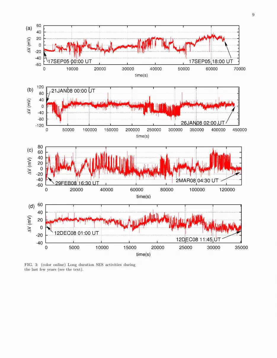
In Fig.3 the following four long duration SES activitiesare depicted all of which have been recorded with sam-pling frequency fexp = 1sample/s at a station close toPirgos (PIR) city located in western Greece (In this sta-tion only electric field variations are continuously moni-tored with a multitude of measuring dipoles the deploy-ment of which has been described in detail in the Sup-plementary Information of Ref.53). First, the SES ac-tivity on September 17, 2005 with duration of severalhours that preceded the Mw6.7 earthquake with an epi-center at 36.3oN23.3oE on January 8, 2006. Second,the SES activity that lasted from January 21 until Jan-uary 26, 2008 and preceded the Mw6.9 earthquake at36.5oN21.8oE on February 14, 2008. Third, the SESactivity during the period from February 29 to March2, 2008 that was followed32 by a Mw6.4 earthquake at38.0oN21.5oE on June 8, 2008 (SES activity informationis issued only when the expected magnitude is around 6units or larger44,53). Finally, Fig.3(d) depicts the mostrecent SES activity of duration of several hours that wasrecorded on December 12, 2008. The latter SES activity

4

was followed by a Mw5.4 earthquake at 37.1oN20.8oEon February 16, 2009 (according to Athens Observa-tory the magnitude is Ms(ATH)=ML+0.5=6.0; we clar-ify that predictions are issued only when the expectedmagnitude is comparable to 6.0 units or larger). Notethat this earthquake occurred after the initial submis-sion of the present paper (and its time of occurrence wasapproached54 by means of the procedure developed inRef.32).

Here, we analyze, as an example, the long durationSES activity that lasted from February 29 until March2, 2008(Fig.3(c)). The time-series of this electrical dis-turbance, which is not of obvious dichotomous nature,is depicted in the upper channel (labelled “a”) of Fig.4.The signal, comprising a number of pulses, is superim-posed on a background which exhibits frequent small MTvariations. The latter are simultaneously recorded at allmeasuring sites, in contrast to the SES activities thatsolely appear at a restricted number of sites dependingon the epicentral region of the future earthquake39. Thisdifference provides a key for their distinction. In order toseparate the background, we proceed into the followingsteps: First, we make use of another measuring dipole ofthe same station, i.e., the channel labelled “b” in Fig.4,which has not recorded the signal but does show the MTpseudo-sinusoidal variations. Second, since the samplingrate of the measurements is 1sample/s, we now computethe increments every 1s of the two time-series of channels“a” and “b”. Assuming the “1s increments” of channel“a” lying along the x-axis and those of “b” along the y-axis, we plot in the middle panel of Fig.4 (labeled “c”)the angle of the resulting vector with dots. When a non-MT variation (e.g., a dichotomous pulse) appears (disap-pears) in channel “a”, this angle in “c” abruptly changesto 0o (±180o). Thus, the dots in panel “c” mark suchchanges. In other words, an increased density of dots(dark regions) around 0o or ±180o marks the occurrenceof these pulses, on which we should focus. To this end,we plot in channel “d” of Fig.4 the residual of a linearleast squares fit of channel “a” with respect to channel“b”. Comparing channel “d” with channel “a”, we noticea significant reduction of the MT background but not ofthe signal. The small variations of the MT backgroundthat still remain in “d”, are now marked by the light blueline, which when removed result in channel “e” of Fig.4.Hence, channel “e” solely contains the electric field vari-ations that precede rupture. This channel provides thetime-series which should now be analyzed.

The DFA analysis (in conventional time) of the time-series of channel “e” of Fig.4 is shown in Fig.5. Itreveals an almost linear logF (n) vs logn plot (wheren = fexp∆t) with an exponent α ≈ 1 practically over all

scales available (approximately five orders of magnitude).Note, that this value of the exponent remains the sameirrespective if we apply DFA-1, DFA-2 or DFA-3. Thisresult is in agreement with the results obtained25,26,40,41

for SES activities of shorter duration.

For the classification of this signal, i.e., to distinguish

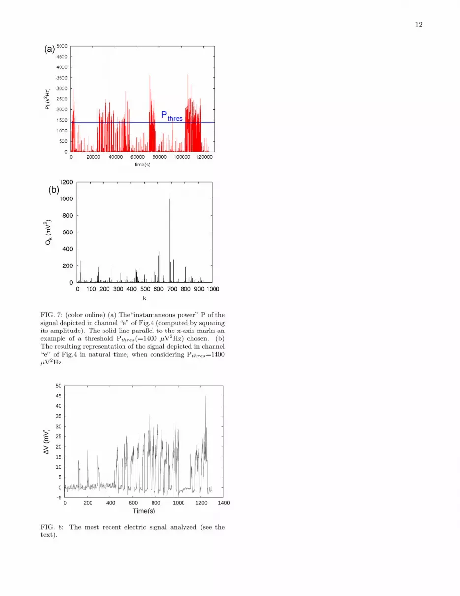
whether it is a true SES activity or a man-made electricsignal, we now proceed to its analysis in natural time. Inorder to define (χk, Qk) the individual pulses of the sig-nal depicted in channel “e” of Fig.4 have to be identified.A pulse starts, of course, when the amplitude exceeds agiven threshold and ends when the amplitude falls belowit. Moreover, since the signal is not obviously dichoto-mous, instead of finding the duration of each pulse, oneshould sum the “instantaneous power” during the pulseduration in order to find Qk, as already mentioned. Tothis end, we plot in Fig.6 the histogram of the instan-taneous power P of channel “e” of Fig.4, computed bysquaring its amplitude. An inspection of this figure re-veals a bimodal feature which signifies the periods of in-activity (P< 500µV2Hz) and activity (P> 500µV2Hz)in channel “e” of Fig.4. In order to find Qk, we focuson the periods of activity and select the power thresholdPthres around the second peak of the histogram in Fig.6.Let us consider, for example, the case of Pthres=1400µV2Hz. In Fig.7(a), we depict the instantaneous powerP of the signal in channel “e” of Fig.4. Starting fromthe beginning of the signal, we compare P with Pthres

and when P exceeds Pthres we start summing up the Pvalues until P falls below Pthres for the first time, k = 1.The resulting sum corresponds to Q1. This procedure isrepeated until P falls below Pthres for the second time,k = 2, and the new sum represents Q2, etc. This leadsto the natural time representation depicted in Fig.7(b).The result depends, of course, on the proper selection ofPthres. The latter can be verified by checking whether asmall change of Pthres around the second peak of the his-togram, leads to a natural time representation resultingin approximately the same values of the parameters κ1, Sand S−. By randomly selecting Pthres in the range 500 to2000 µV2Hz, we obtain that the number of pulses in chan-nel “e” of Fig.4 is N = 1100±500 with κ1 = 0.070±0.007,S = 0.082± 0.012 and S− = 0.078± 0.006. When Pthres

ranges between 1000 to 1500 µV2Hz, the correspondingvalues are N = 1200 ± 200 with κ1 = 0.068 ± 0.003,S = 0.080± 0.005 and S− = 0.074± 0.003. Thus, we ob-serve that irrespective of the Pthres value chosen, the pa-rameters κ1, S and S− obey the conditions (8) and (9) forthe classification of this signal as SES activity. The sameholds for a non-dichotomous signal recorded on March 28,2009 at Keratea station located close to Athens (Fig.8).To approach the occurrence time of the impending event,the procedure developed in Ref.32 has been employed forthe seismicity within the area N38.8

37.7E24.122.6. The results,

when considering the seismicity until early in the morn-ing on June 19, 2009, are shown in Fig.9. They showthat a local maximum of the probability32 Prob(κ1) ofthe seismicity is observed at κ1 = 0.070 upon the occur-rence of the following events: (a) an ML=3.2 event at12:42 UT on June 18 with epicenter at 38.7N 23.0E andan ML=3.2 event at 03:44 UT on June 19 at 37.9N 23.0Eif we take a magnitude threshold Mthres=3.0 (b) whentaking Mthres=3.1, the maximum occurs again upon theoccurrence of the aforementioned event at 12:42 on June

5

18 (c) when increasing the threshold at Mthres=3.2, themaximum occurs somewhat earlier, i.e., upon the oc-currence of the ML=3.5 event at 08:26 UT on June 18at 38.7N 23.0E. Let us now consider a larger area, i.e.,N39.00

37.65E24.1022.20, and repeat the same calculation. The re-

sults are shown in Fig.10. They reveal again the occur-rence of a local maximum of Prob(κ1) at κ1 = 0.070 uponthe occurrence of the above mentioned ML=3.2 event at12:42 UT on June 18 when considering either Mthres=3.2(Fig.10(c)) or Mthres=3.1 (Fig.10(b)) (for the latter casea maximum also occurs at the last event shown in thefigure with ML=3.2 at 03:44 UT on June 19). Themaximum appears upon the occurrence of a ML=3.0 at23:48 UT on June 18 when decreasing the threshold atMthres=3.0.

In summary, the results exhibit both magnitude- andspatial- invariance, which is characteristic when ap-proaching the critical point.

Note added on July 21, 2009. Repeating the aforemen-tioned calculation for the area N39.00

37.65E24.1022.20, we find the

results depicted in Fig.11(a) for Mthres=2.8. An inspec-tion of this figure reveals a local maximum of Prob(κ1)at κ1 = 0.070 upon the occurrence of a ML=3.0 at 21:10UT on July 19, 2009 with an epicenter at 38.1N 22.7E(the same result is found for Mthres=2.9.) Interestingly,this local maximum turns to be the prominent one whenstudying the seismicity in the same area (for the samethreshold Mthres=2.8) since June 21, 2009, see Fig.11(b);the same holds for Mthres=3.0. Furthermore, the lat-ter study was made for the smaller area N38.8

37.7E24.122.6 for

Mthres= 2.6, 2.7 and 3.0 and showed a local maximumof Prob(κ1) at κ1 = 0.070 upon the occurrence of thesame event (i.e., at 21:10 UT on July 19, 2009). The in-vestigation still continues in order to clarify whether thelatter local maximum will eventually turn to become aprominent one.

Note added on September 5, 2009. At 8:17 UT onSeptember 2, 2009, a ML=4.3 earthquake occurred al-most at the center of the predicted area N38.8

37.7E24.122.6. The

continuation of the investigation of the previous para-graph in the smaller area N38.8

37.7E24.122.6 showed a prominent

maximum of Prob(κ1) at κ1 = 0.070 (see Fig.12 (a))upon the occurrence of a ML=3.3 event at 09:35 UT onSeptember 2, 2009, with an epicenter at 38.1N 23.3E.This was found to hold for the aforementioned larger area(see Fig.12 (b)) as well, thus revealing that the criticalitycondition -as developed in Ref. 32- is obeyed.

Note added on September 19, 2009. The previous Notewas followed by three earthquakes of magnitude 4.4, 4.7and 4.8 that occurred at 21:15 UT September 9, 06:04UT September 10 and 07:12 UT September 16, 2009 withepicenters at 38.7N 22.8E, 38.3N 24.1E and 39.0N 22.2E,respectively. The continuation of the natural time inves-tigation of the seismicity for Mthres=3.0 in the smallerarea N38.8

37.7E24.122.6 revealed a prominent maximum Prob(κ1)

at κ1 = 0.070 (see Fig.13 (a)) upon the occurrence of aML=3.0 event at 01:55 UT on September 18, 2009, withepicenter at 38.7N22.8E. Since the same was found to be

true for the aforementioned larger area as well (see Fig.13(b)), the investigation is now extended to additional mag-nitude thresholds in order to clarify whether (beyondspatial and) magnitude threshold invariance holds, thusidentifying that the system approaches the critical point.

Note added on October 13, 2009. The previous notewas actually followed by an earthquake of magnitude4.6 that occurred at 22:27 UT on October 2, 2009 withan epicenter at 38.3N 22.9E. The natural time investi-gation of the seismicity still continues with the follow-ing results. First, in the smaller area N38.8

37.7E24.122.6: For

Mthres=2.7, the criticality condition started to be ap-proached since October 7 and the most prominent max-imum of Prob(κ1) at κ1 = 0.070 was observed upon theoccurrence of the ML=2.7 event at 01:56 UT on October11, 2009. The same behavior was found for Mthres=2.8(but the last event for this case occurred at 08:15UT onOctober 10, 2009 at 38.2N 23.1E). Second, in the largerarea N39.00

37.65E24.1022.20: For both thresholds Mthres=2.7 and

Mthres=2.8, the criticality condition was also started tobe approached since 20:18 UT on October 7, 2009. Themost prominent maximum of Prob(κ1) at κ1 = 0.070 forMthres=2.7 have been observed upon the occurrence ofthe aforementioned ML=2.7 event at 01:56 UT on Oc-tober 11, 2009, while for Mthres=2.8 it was observed at4:51 UT on October 9, 2009, upon the occurrence of theML=2.9 event at 38.1E 23.2E. Interestingly, the resultsfor the larger area are almost identical if the investigationstarts at 15:00 UT on July 31, 2009.

Note added on November 14, 2009. Meanwhile, twoSES activities were recorded at PAT on October 24 andNovember 11, 2009, see Fig.14. Hence, the ongoing study(Fig.15) of the previous Note should be accompanied bya complementary study, focused on the determination ofthe occurrence time of the impending mainshock, thatalso considers the seismicity in the western part (i.e.,N38.6

37.5E22.219.8) of the PAT selectivity map (see area A in

Fig.8 of Ref.32). Such a complementary study, whentaking into account the seismic data until early in themorning on November 13, 2009, leads to the results de-picted in Fig.16 for Mthres=3.1. A local maximum ofProb(κ1) at κ1 = 0.070 was observed (see the rightmostarrow in Fig.16) upon the occurrence of ML=3.2 eventat 18:55 UT on November 2, 2009 (that was followed bya ML=5.6 EQ at 05:25 UT on November 3, 2009, withan epicenter at 37.4oN 20.4oE). In addition, the most

prominent maximum in Fig.16 of Prob(κ1) at κ1 = 0.070is observed later, i.e., upon the occurrence of a ML=3.1event at 01:42 UT on November 13, 2009 (see the left-most arrow in Fig.16). This, which has been also checkedfor Mthres=3.0, provides evidence that the critical pointis approached. Calculations are now carried out to fur-ther investigate the magnitude threshold invariance ofthis behavior.

Note added on November 27, 2009. Actually, after theprevious Note the following two earthquakes occurred at18:30 UT on November 16, 2009 and at 04:29 UT onNovember 19, 2009 with magnitudes (Ms(ATH)) 4.3 and

6

4.4 and epicenters at 38.4oN 22.0oE and 38.2oN 22.7oE,respectively, that both lie within the PAT selectivitymap, i.e, N38.6

37.5E23.319.8. The continuation of the two studies

mentioned in the previous Note, i.e., in the PAT selectiv-ity map as well as in the area N39.00

37.65E24.122.2, both show that

the most prominent maximum of Prob(κ1) at κ1 = 0.070was observed upon the occurrence of the ML=3.2 eventat 19:31 UT on November 25, 2009, thus indicating thatthe system is near the critical point.Note added on February 9, 2010. Two earthquakes

with magnitudes Ms(ATH)(= ML+0.5)=5.7 and 5.6 oc-curred at 38.4oN 22.0oE (and hence inside the expectedarea) at 15:56 UT on January 18 and at 00:46 UT on Jan-uary 22, 2010 (after observing a maximum of Prob(κ1)versus κ1 at κ1=0.070 for Mthres=3.1 upon the occur-rence of the ML=3.2 event at 15:56 UT on January 15,2010). These two magnitudes are consistent with the con-dition Ms(ATH)≥6.0 (under which SES information arepublicized) if a reasonable55 experimental error 3σ=0.7is accepted.However, since the amplitudes of all the SES activ-

ities recorded could warrant an impending mainshockwith magnitude exceeding Ms(ATH)=6.0, and in orderto determine the occurrence time of such a mainshock, ifany, the natural time analysis of seismicity still contin-ues. This analysis starting at 04:00 UT on December 27,2009, revealed that in the area N39.0

38.0E23.721.5 (almost 200km

× 100km) the criticality condition (i.e., Prob(κ1) ver-sus κ1 maximizes at κ1=0.070) for Mthres=3.5 is obeyedduring the last three events of Fig.17, the latest of which(that exhibits the strongest maximum) occurred at 10:18UT on February 7, 2010 at 38.6oN 23.7oE with ML=4.3.This has been checked to be valid for broader areas aswell (spatial invariance), but has not yet been found tobe confirmed (until early in the morning on February8, 2010) for lower magnitude thresholds. The investiga-tion of the latter is still in progress, because the followingmight happen: Due to coarse-graining the criticality con-dition might have been obeyed at a larger time-windowfor large magnitude thresholds, while for smaller thresh-olds the time-window may become smaller thus achievinga better accuracy in the determination of the occurrencetime of the impending earthquake.

IV. DISCUSSION

In general, electric field variations are interconnectedwith the magnetic field ones through Maxwell equations.Thus, it is intuitively expected that when the former ex-hibit long range correlations the same should hold for thelatter. This expectation is consistent with the presentfindings which show that, at long time-lags, the originaltime-series of both electric- and magnetic field variations

preceding rupture exhibit DFA-exponents close to unity.The above can be verified when data of both electric-

and magnetic-field variations are simultaneously avail-able. This was the case of the data presented in Fig.1.In several occasions, however, as mentioned in Section I,only magnetic field data exist, in view of the fact that it iseasier to conduct magnetic field measurements comparedto the electric field ones. When using coil magnetome-ters, the magnetic field variations have the form of seriesof ‘spikes’. Whenever the amplitude of these ‘spikes’ sig-nificantly exceed the pseudo-sinusoidal variations of theMT background, as in the case of BEW in Fig.1, a di-rect application of DFA (see Fig.2) elucidates the longrange correlations in the magnetic field variations pre-ceding rupture. On the other hand, when considerablepseudo-sinusoidal MT variations are superimposed, a di-rect application of DFA is not advisable. One must firstsubtract the MT variations (following a procedure sim-ilar to that used in the electric field data in Fig.4) andthen apply DFA.The preceding paragraph refers to the analysis of the

signal in conventional time. As already shown in Ref.41,natural time analysis, has the privilege that allows thedistinction between true SES activities and man madesignals. This type of analysis, however, demands theknowledge of the energy released during each consecu-tive event. The determination of this energy is easierto conduct in the case of electric field variations (thisis so, because coil magnetometers, as mentioned in Sec-tion II, act as dB/dt detectors). When these variationsare of clear dichotomous nature, the energy release isproportional to the duration of each pulse40,41. On theother hand, in absence of an obvious dichotomous naturean analysis of the ‘instantaneous power’ similar to thatpresented in the last paragraph of Section III should becarried out to determine the parameters κ1, S and S− innatural time.

V. CONCLUSIONS

First, DFA was used as a scaling analysis method toinvestigate long-range correlations in the original timeseries of the magnetic field variations that precede rup-ture and have the form of ‘spikes’ of alternating sign. Wefind a scaling exponent α close to 0.9 for time-lags largerthan the average time interval 〈T 〉 between consecutive‘spikes’, while at shorter time-lags the exponent is closeto 0.5 thus corresponding to uncorrelated behavior.Second, using electric field data of long duration SES

activities (i.e., from several hours to a couple of days)recorded during the last few years, DFA reveals a scaleinvariant feature with an exponent α ≈ 1, over all scalesavailable (approximately five orders of magnitude).

∗ Electronic address: pvaro@otenet.gr 1 C.-K. Peng, J. Mietus, J. M. Hausdorff, S. Havlin, H. E.

7

Stanley, and A. L. Goldberger, Phys. Rev. Lett. 70, 1343(1993).

2 C.-K. Peng, S. V. Buldyrev, S. Havlin, M. Simons, H. E.Stanley, and A. L. Goldberger, Phys. Rev. E 49, 1685(1994).

3 S. V. Buldyrev, A. L. Goldberger, S. Havlin, R. N. Man-tegna, M. E. Matsa, C.-K. Peng, M. Simons, and H. E.Stanley, Phys. Rev. E 51, 5084 (1995).

4 M. S. Taqqu, V. Teverovsky, and W. Willinger, Fractals 3,785 (1995).

5 P. Talkner and R. O. Weber, Phys. Rev. E 62, 150 (2000).6 K. Hu, P. C. Ivanov, Z. Chen, P. Carpena, and H. E. Stan-ley, Phys. Rev. E 64, 011114 (2001).

7 Z. Chen, P. C. Ivanov, K. Hu, and H. E. Stanley, Phys.Rev. E 65, 041107 (2002).

8 Z. Chen, K. Hu, P. Carpena, P. Bernaola-Galvan, H. E.Stanley, and P. C. Ivanov, Phys. Rev. E 71, 011104 (2005).

9 L. Xu, P. C. Ivanov, K. Hu, Z. Chen, A. Carbone, andH. E. Stanley, Phys. Rev. E 71, 051101 (2005).

10 S. M. Ossadnik, S. B. Buldyrev, A. L. Goldberger,S. Havlin, R. N. Mantegna, C. K. Peng, M. Simons, andH. E. Stanley, Biophys. J. 67, 64 (1994).

11 R. N. Mantegna, S. V. Buldyrev, A. L. Goldberger,S. Havlin, , C. K. Peng, M. Simons, and H. E. Stanley,Phys. Rev. Lett. 73, 3169 (1994).

12 R. N. Mantegna, S. V. Buldyrev, A. L. Goldberger,S. Havlin, , C. K. Peng, M. Simons, and H. E. Stanley,Phys. Rev. Lett. 76, 1979 (1996).

13 P. Carpena, P. Bernaola-Galvan, P. C. Ivanov, and H. E.Stanley, Nature (London) 418, 955 (2002).

14 K. Hu, P. C. Ivanov, Z. Chen, M. F. Hilton, H. E. Stanley,and S. A. Shea, Physica A 337, 307 (2004).

15 J. M. Hausdorff, Y. Ashkenazy, C. K. Peng, P. C. Ivanov,H. E. Stanley, and A. L. Goldberger, Physica A 302, 138(2001).

16 Y. Ashkenazy, J. M. Hausdorff, P. C. Ivanov, and H. E.Stanley, Physica A 316, 662 (2002).

17 P. C. Ivanov, A. Bunde, L. A. Nunes Amaral, S. Havlin,J. Fritsch-Yelle, R. M. Baevsky, H. E. Stanley, and A. L.Goldberger, Europhys. Lett. 48, 594 (1999).

18 S. Havlin, S. V. Buldyrev, A. Bunde, A. L. Goldberger,P. C. Ivanov, C. K. Peng, and H. E. Stanley, Physica A273, 46 (1999).

19 H. E. Stanley, L. A. Nunes Amaral, A. L. Goldberger,S. Havlin, P. C. Ivanov, and C. K. Peng, Physica A 270,309 (1999).

20 P. C. Ivanov, L. A. Nunes Amaral, A. L. Goldberger, andH. E. Stanley, Europhys. Lett. 43, 363 (1998).

21 K. Ivanova and M. Ausloos, Physica A 274, 349 (1999).22 K. Ivanova, T. P. Ackerman, E. E. Clothiaux, P. C.

Ivanov, H. E. Stanley, and M. Ausloos, J. Geophys. Res.-Atmospheres 108 D9, 4268 (2003).

23 E. Koscielny-Bunde, A. Bunde, S. Havlin, H. E. Roman,Y. Goldreich, and H. J. Schellnhuber, Phys. Rev. Lett. 81,729 (1998).

24 R. L. Stratonovich, Topics in the theory of random noise

Vol. I (Gordon and Breach, New York, 1981).25 P. A. Varotsos, N. V. Sarlis, and E. S. Skordas, Phys. Rev.

E 66, 011902 (2002).26 A. Weron, K. Burnecki, S. Mercik, and K. Weron, Phys.

Rev. E 71, 016113 (2005).27 P. Varotsos and K. Alexopoulos, Tectonophysics 110, 73

(1984).28 A. C. Fraser-Smith, A. Bernardi, P. R. McGill, M. E. Ladd,

R. A. Helliwell, and O. G. Villard, Geophys. Res. Lett. 17,1465 (1990).

29 S. Uyeda, T. Nagao, Y. Orihara, T. Yamaguchi, andI. Takahashi, Proc. Natl. Acad. Sci. USA 97, 4561 (2000).

30 S. Uyeda, M. Hayakawa, T. Nagao, O. Molchanov, K. Hat-tori, Y. Orihara, K. Gotoh, Y. Akinaga, and H. Tanaka,Proc. Natl. Acad. Sci. USA 99, 7352 (2002).

31 P. A. Varotsos, N. V. Sarlis, H. K. Tanaka, and E. S. Sko-rdas, Phys. Rev. E 72, 041103 (2005).

32 N. V. Sarlis, E. S. Skordas, M. S. Lazaridou, and P. A.Varotsos, Proc. Japan Acad., Ser. B 84, 331 (2008).

33 P. Varotsos, K. Alexopoulos, and K. Nomicos, Phys. StatusSolidi B 111, 581 (1982).

34 D. Kostopoulos, P. Varotsos, and S. Mourikis, Can. J.Phys. 53, 1318 (1975).

35 P. Varotsos, J. Phys. Chem. Sol. 42, 405 (1981).36 P. Varotsos and K. Alexopoulos, J. Phys. Chem. Sol. 41,

443 (1980).37 P. Varotsos and K. Alexopoulos, Phys. Status Solidi B 42,

409 (1981).38 P. Varotsos and K. Alexopoulos, Phys. Rev. B 21, 4898

(1980).39 P. Varotsos and K. Alexopoulos, Thermodynamics of Point

Defects and their Relation with Bulk Properties (NorthHolland, Amsterdam, 1986).

40 P. A. Varotsos, N. V. Sarlis, and E. S. Skordas, Phys. Rev.E 67, 021109 (2003).

41 P. A. Varotsos, N. V. Sarlis, and E. S. Skordas, Phys. Rev.E 68, 031106 (2003).

42 P. A. Varotsos, N. V. Sarlis, E. S. Skordas, and M. S.Lazaridou, Phys. Rev. E 70, 011106 (2004).

43 P. A. Varotsos, N. V. Sarlis, H. K. Tanaka, and E. S. Sko-rdas, Phys. Rev. E 71, 032102 (2005).

44 P. A. Varotsos, N. V. Sarlis, E. S. Skordas, H. K. Tanaka,and M. S. Lazaridou, Phys. Rev. E 73, 031114 (2006).

45 B. Lesche, J. Stat. Phys. 27, 419 (1982).46 B. Lesche, Phys. Rev. E 70, 017102 (2004).47 P. A. Varotsos, N. V. Sarlis, and E. S. Skordas, Phys. Rev.

Lett. 91, 148501 (2003).48 N. Sarlis and P. Varotsos, J. Geodyn. 33, 463 (2002).49 D. Karakelian, G. C. Beroza, S. L. Klemperer, and A. C.

Fraser-Smith, Bull. Seism. Soc. Am. 92, 1513 (2002).50 O. A. Molchanov, Y. A. Kopytenko, P. M. Voronov, E. A.

Kopytenko, T. G. Matiashvili, A. C. Fraser-Smith, andA. Bernardi, Geophys. Res. Lett. 19, 1495 (1992).

51 P. Varotsos, N. Sarlis, and E. Skordas, Proc. Jpn. Acad.,Ser. B: Phys. Biol. Sci. 77, 87 (2001).

52 P. A. Varotsos, N. V. Sarlis, and E. S. Skordas, Appl. Phys.Lett. 86, 194101 (2005).

53 P. A. Varotsos, N. V. Sarlis, E. S. Skordas, H. K. Tanaka,and M. S. Lazaridou, Phys. Rev. E 74, 021123 (2006).

54 P. A. Varotsos, N. V. Sarlis, E. S. Skordas, and M. S.Lazaridou (2009), cond-mat/0707.3074v3.

55 P. Varotsos, The Physics of Seismic Electric Signals (Ter-raPub, Tokyo, 2005).

8

10:00:00 11:30:00 13:00:00 14:30:00

10.0

10.0

6.0

6.0

6.0

BEW

BNS

Ec−W

c

Nc−S

c

L‘s−I

IOANNINA Station 18 April 1995m

V p

er d

ivis

ion

mV

/km

per

div

isio

n

12:00:25 12:02:25 12:04:25 12:06:25 12:08:25

6.0

6.0

3.0

3.0

3.0

BEW

BNS

Ec−W

c

Nc−S

c

L‘s−I

IOANNINA Station 18 April 1995

mV

per

div

isio

n m

V/k

m p

er d

ivis

ion

(a)

(b)

FIG. 1: (a):Variations of the electric- (upper three channels)and magnetic- (lower two channels) field recorded on April18, 1995 (see the text). (b):A 10min excerpt of (a). The twodashed lines in (a) show the excerpt depicted in (b).

-1

-0.5

0

0.5

1

1.5

2

0.5 1 1.5 2 2.5 3 3.5

log

F(n

)

log n

αDFA=0.52αDFA=0.89

FIG. 2: (color online)The DFA for the BEW channel ofFig.1(a). Logarithm base 10 is used.

9

FIG. 3: (color online) Long duration SES activities duringthe last few years (see the text).

10

FIG. 4: (color online) The long duration SES activity fromFebruary 29 to March 2, 2008. Channel “a”:original timeseries, channel “b”: recordings at a measuring dipole whichdid not record the SES activity, but does show MT variations,“c”:the angle of the resulting vector upon assuming that the“1s increments” of channel “a” lie along the x-axis and thoseof channel “b” along the y-axis. Channel “d”: the residual of alinear least squares fit of channel “a” with respect to channel“b”, channel “e”:the same as “d” but after eliminating theslight variations of the background. For the sake of clarity,channels “a”, “b” and “d” have been shifted vertically.

11

0

0.5

1

1.5

2

2.5

3

3.5

4

4.5

0.5 1 1.5 2 2.5 3 3.5 4 4.5 5

log

F(n

)

log n

DFA-1DFA-2DFA-3

αDFA=1.05

FIG. 5: (color online) The DFA-l (l=1,2 and 3) for the lowerchannel (i.e., the one labelled “e”) of Fig.4. Logarithm base10 is used.

1

10

100

1000

10000

100000

0 500 1000 1500 2000 2500 3000 3500 4000 4500

Fre

quen

cy

P (µV2Hz)

FIG. 6: Histogram of the “instantaneous power” P, i.e., thesquared amplitude of the signal depicted in channel “e” ofFig.4.

12

FIG. 7: (color online) (a) The“instantaneous power” P of thesignal depicted in channel “e” of Fig.4 (computed by squaringits amplitude). The solid line parallel to the x-axis marks anexample of a threshold Pthres(=1400 µV2Hz) chosen. (b)The resulting representation of the signal depicted in channel“e” of Fig.4 in natural time, when considering Pthres=1400µV2Hz.

-5

0

5

10

15

20

25

30

35

40

45

50

0 200 400 600 800 1000 1200 1400

∆V (

mV

)

Time(s)

FIG. 8: The most recent electric signal analyzed (see thetext).

13

4

6

8

10

12

14

16

18

No of EQs after SES

0.000.02

0.040.06

0.080.10

0.120.14

κ1

0.1

0.2

0.3

0.4

0.5

Pro

b(κ 1

)

46

810

1214

1618

2022

2426

No of EQs after SES

0.000.02

0.040.06

0.080.10

0.120.14

κ1

0.1

0.2

0.3

0.4

0.5

Pro

b(κ 1

)

46

810

1214

1618

2022

2426

2830

3234

3638

4042

No of EQs after SES

0.000.02

0.040.06

0.080.10

0.120.14

κ1

0.1

0.2

0.3

0.4

0.5

Pro

b(κ 1

)(a) Mthres =3.0

(c) M thres =3.2

(b) Mthres =3.1

FIG. 9: The probability Prob(κ1) of the seismicity withinthe area N38.8

37.7E24.1

22.6 subsequent to the SES activity recordedat KER on March 28, 2009, when considering the followingmagnitude thresholds: Mthres=3.0 (a), 3.1 (b) and 3.2 (c).

14

46

810

1214

1618

2022

24

No of EQs after SES

0.000.02

0.040.06

0.080.10

0.120.14

κ1

0.1

0.2

0.3

0.4

0.5

Pro

b(κ 1

)

46

810

1214

1618

2022

2426

2830

3234

3638

No of EQs after SES

0.000.02

0.040.06

0.080.10

0.120.14

κ1

0.1

0.2

0.3

0.4

0.5

Pro

b(κ 1

)

46810121416182022242628303234363840424446485052545658606264

No of EQs after SES

0.000.02

0.040.06

0.080.10

0.120.14

κ1

0.1

0.2

0.3

0.4

0.5

Pro

b(κ 1

)(a) Mthres =3.0

(c) M thres =3.2

(b) Mthres =3.1

FIG. 10: The same as Fig.9, but for the area N39.00

37.65E24.10

22.20 inorder to check the spatial invariance of the results (see thetext).

15

46

810

1214

1618

2022

2426

No of EQs after SES

0.000.02

0.040.06

0.080.10

0.120.14

κ1

0.1

0.2

0.3

0.4

0.5

Pro

b(κ

1)

20

40

60

80

100

120

140

160

180

No of EQs after SES

0.000.02

0.040.06

0.080.10

0.120.14

κ1

0.1

0.2

0.3

0.4

0.5

Pro

b(κ 1

)(a)

(b)

FIG. 11: The same as Fig.9, but for the area N39.00

37.65E24.10

22.20 byconsidering the seismicity since (a) March 28, 2009 and (b)June 21, 2009 (see the text).

16

46

810

1214

1618

2022

2426

2830

3234

3638

40

No of EQs after SES

0.000.02

0.040.06

0.080.10

0.120.14

κ1

0.1

0.2

0.3

0.4

0.5

Pro

b(κ 1

)

4681012

1416

1820

2224

2628

3032

3436

3840

4244

4648

5052

5456

No of EQs after SES

0.000.02

0.040.06

0.080.10

0.120.14

κ1

0.1

0.2

0.3

0.4

0.5

Pro

b(κ 1

)(a)

(b)

FIG. 12: The probability Prob(κ1) vs κ1 upon consideringthe seismicity (Mthres=3.1) until 9:35 UT on September 2,2009: Panel (a) corresponds to the area N38.8

37.7E24.1

22.6, whereaspanel (b) to the larger area N39.00

37.65E24.10

22.20.

17

468101214161820222426283032343638404244464850525456586062646668707274767880828486889092949698100102

104106

108110

No of EQs after SES

0.000.02

0.040.06

0.080.10

0.120.14

κ1

0.1

0.2

0.3

0.4

0.5

Pro

b(κ 1

)

468101214161820222426283032343638404244464850525456586062646668707274

No of EQs after SES

0.000.02

0.040.06

0.080.10

0.120.14

κ1

0.1

0.2

0.3

0.4

0.5

Pro

b(κ 1

)κ 1

Pro

b(

)κ 1

Pro

b(

)(a)

(b)

FIG. 13: The probability Prob(κ1) vs κ1 upon consideringthe seismicity (Mthres=3.0) until 1:55 UT on September 18,2009: Panel (a) corresponds to the area N38.8

37.7E24.1

22.6, whereaspanel (b) to the larger area N39.00

37.65E24.1022.20.

18

0 500 1000 1500 20000

100

200

300∆V

(m

V)

0 2000 4000 6000 8000 1000050

100

150

200

250

300

time (s)

∆V (

mV

)PAT 24 Oct. 2009

PAT 11 Nov. 2009

FIG. 14: The SES activities at PAT on 24 October 2009 (up-per) and 11 November 2009 (lower), see the text.

21˚E 22˚E 23˚E 24˚E 25˚E 26˚E

37˚N

38˚N

39˚N

40˚N

21˚E 22˚E 23˚E 24˚E 25˚E 26˚E

37˚N

38˚N

39˚N

40˚N

21˚E 22˚E 23˚E 24˚E 25˚E 26˚E

37˚N

38˚N

39˚N

40˚N

21˚E 22˚E 23˚E 24˚E 25˚E 26˚E

37˚N

38˚N

39˚N

40˚N

March 31, 2009

May 17, 2009

May 17, 2009

May 29, 2009

June 17, 2009

September 2, 2009

September 10, 2009

September 16, 2009

October 2, 2009

October 26, 2009

November 12, 2009

21˚E 22˚E 23˚E 24˚E 25˚E 26˚E

37˚N

38˚N

39˚N

40˚N

LAM

KER

VOL

PIRLOU

ATHPAT

21˚E 22˚E 23˚E 24˚E 25˚E 26˚E

37˚N

38˚N

39˚N

40˚N

FIG. 15: Earthquakes with magnitude Ms(ATH)≥4.5 andepicenters within (or very close to) the area(s) specified inadvance that followed the consecutive Notes added to thispaper.

19

8

10

12

14

16No of EQs after SES

0.000.02

0.040.06

0.080.10

0.120.14

κ1

0.1

0.2

0.3

0.4

0.5

Pro

b(κ 1

)

2 Nov 2009 18:55 UT13 Nov 2009 1:42 UT

FIG. 16: The probability Prob(κ1) of the seismicity withinthe area N38.6

37.5E23.3

19.8 subsequent to the SES activity recordedat PAT on October 24, 2009, when considering Mthres=3.1.The seismic data until early in the morning on November 13,2009, have been used.

20

4

6

8

10

12

14

16

18

No of EQs after SES

0.000.02

0.040.06

0.080.10

0.120.14

κ1

0.1

0.2

0.3

0.4

0.5

Pro

b(κ 1

)

EQ No.18: 7 Feb 2010, 10:18 UT ML 4.3EQ No.17: 30 Jan 2010, 13:47 UT ML 4.4EQ No.16: 22 Jan 2010, 18:14 UT ML 3.8

FIG. 17: The probability Prob(κ1) of the seismicity, forMthres=3.5, within the area N39.0

38.0E23.7

21.5 when considering theseismic data until early in the morning on February 8, 2010.