Embed Size (px)
Citation preview

NOTE TO USERS
This reproduction is the best copy available.
UMI


mn u Ottawa
L'Universite canadienne Canada's university

mn FACULTE DES ETUDES SUPERIEURES 1 ^ = 1 FACULTY OF GRADUATE AND
ET POSTOCTORALES U Ottawa POSDOCTORAL STUDIES r,'Univcisit6 oanadienne
Canada's university
Chaoyang Feng AUTEUR DE LA THESE / AUTHOR OF THESIS
Ph.D. (Chemical Engineering) GRADE/DEGREE
Department of Chemical Engineering TACliltTrEColFblPW
Development of Novel Nanofiber Membranes for Seawater Desalination by Air Gap Membrane Distillation
TITRE DE LA THESE / TITLE OF THESIS
Takeshi Matsuura DIRECTEUR (DIRECTRICE) DE LA THESE / THESIS SUPERVISOR
CO-DIRECTEUR (CO-DIRECTRICE) DE LA THESE / THESIS CO-SUPERVISOR
EXAMINATEURS (EXAMINATRICES) DE LA THESE/THESIS EXAMINERS
Christopher Lan Andre Tremblay
Arturo Macchi Remi Lebrun
Gary W. Slater Le Doyen de la Faculte des etudes superieures et postdoctorales / Dean of the Faculty of Graduate and Postdoctoral Studies

DEVELOPMENT OF NOVEL NANOFIBER
MEMBRANES FOR SEAWATER DESALINATION BY
AIR GAP MEMBRANE DISTILLATION
By
Chaoyang Feng
Ph.D. Thesis
A thesis submitted to the Faculty of Graduate and Postdoctoral Studies in
partial fulfillment of the requirements for the degree of
Ph.D. in Chemical and Biological Engineering
Under the Supervision of:
Professor Takeshi Matsuura of University of Ottawa, Canada
Department of Chemical and Biological Engineering
University of Ottawa
Ottawa, ON
Canada, KIN 6N5
© Chaoyang Feng, Ottawa, Canada, 2009

1*1 Library and Archives Canada
Published Heritage Branch
395 Wellington Street Ottawa ON K1A 0N4 Canada
Bibliotheque et Archives Canada
Direction du Patrimoine de I'edition
395, rue Wellington Ottawa ON K1A 0N4 Canada
Your file Votre rtterence ISBN: 978-0-494-59530-5 Our file Notre reference ISBN: 978-0-494-59530-5
NOTICE: AVIS:
The author has granted a nonexclusive license allowing Library and Archives Canada to reproduce, publish, archive, preserve, conserve, communicate to the public by telecommunication or on the Internet, loan, distribute and sell theses worldwide, for commercial or noncommercial purposes, in microform, paper, electronic and/or any other formats.
L'auteur a accorde une licence non exclusive permettant a la Bibliotheque et Archives Canada de reproduire, publier, archiver, sauvegarder, conserver, transmettre au public par telecommunication ou par I'lnternet, preter, distribuer et vendre des theses partout dans le monde, a des fins commerciales ou autres, sur support microforme, papier, electronique et/ou autres formats.
The author retains copyright ownership and moral rights in this thesis. Neither the thesis nor substantial extracts from it may be printed or otherwise reproduced without the author's permission.
L'auteur conserve la propriete du droit d'auteur et des droits moraux qui protege cette these. Ni la these ni des extraits substantiels de celle-ci ne doivent etre imprimes ou autrement reproduits sans son autorisation.
In compliance with the Canadian Privacy Act some supporting forms may have been removed from this thesis.
Conformement a la loi canadienne sur la protection de la vie privee, quelques formulaires secondaires ont ete enleves de cette these.
While these forms may be included in the document page count, their removal does not represent any loss of content from the thesis.
Bien que ces formulaires aient inclus dans la pagination, il n'y aura aucun contenu manquant.
1*1
Canada

Chaoyanq Feng PhD Thesis 2008
Abstract
Our world is facing water and energy shortage. As a relatively new process, membrane
distillation (MD) is being investigated as a low cost and energy saving alternative to
conventional separation processes such as distillation and reverse osmosis since 1990s.
As a result of material limit, the development of membrane distillation has not yet come
to the commercial scale. But, it has become a hopeful technology of the future. The
objective of this research is to develop novel nanofiber membranes for seawater
desalination by air gap membrane distillation (AGMD).
The concept of novel nanofiber membranes is based on the electro-spinning technology.
By using electro-spinning method, a highly hydrophobic material (PVDF, poly
vinylidene fluoride) was spun to filaments with diameters in nanometer range. The PVDF
nanofibers turn into a nanofiber non-woven mat or web and bring high hydrophobicity
and a highly open pore structure. This further fulfils the requirements for the MD
membranes with reduced mass transport resistance and temperature polarization. Thus,
membranes with high MD fluxes are expected.
In Part I of the current research, hydrophilic and hydrophobic polymers and a polymer
blend (PVDF, PVDF/PVP, PS, PES, PEI, PVC, PC, PAN, Nomex (PA), PVA and
Collagen) were used for electro-spinning to generate naonofibers and nanofiber
membranes. The electro-spinning parameters that affect the structure and other properties
of the membrane and the MD membrane performance were identified. They include
spinning dope concentration, solution feed rate, spinning voltage and naonofiber collect
distance. The electro-spinning parameters were then optimized for obtaining the best
performance data.
The PVDF nanofiber membranes were characterized by SEM, AFM, DSC, measurement
of LEPw (liquid entry pressure of water), equilibrium contact angle and particle
separation. It was found that the pore size of the PVDF nanofiber membrane was around
1.5 jam. The equilibrium contact angle of some nanofiber membranes were above 120°. It
II

Chaovanq Feng PhD Thesis 2008
shows that the novel membranes have a very open pore structure and are highly
hydrophobic. Those characteristics are exactly what are needed for MD membranes.
In Part II of the current research work, a novel PVDF nanofiber membrane was tested for
saline water desalination by AGMD (air gap membrane distillation). Desalination by
AGMD was carried out for various sodium chloride concentrations in feed (1 to 22 wt%)
at the feed solution and cooling water temperature difference of 60 °C. Above 99% salt
rejection and above 8 kg/m h flux was obtained. As well, ethanol/water separation was
investigated by using 5 and 10 wt % aqueous ethanol solution.
Two theoretical models were developed to simulate the AGMD process; the first model
was developed to describe the AGMD process based on the mass and heat transfer
through the membrane, while the second model deals with the transfer of volatile
component through the air gap. The experimental flux value fits the second model very
well. It shows that the air gap is the dominating stage for the heat transfer of the AGMD
process.
In an early stage of this work, polypropylene (PP) was chosen to prepare membranes of
high hydrophobicity and high porosity for membrane distillation by a solution casting
method. The results are reported in Appendix I. This method, even though novel, was not
quite appropriate to fabricate membranes with hydrophobicity and porosity high enough
for MD application. Howevere, the microporous PP membranes so prepared seem to have
a great potential for other separation applications than MD.
Ill
Chaoyanq Feng PhD Thesis 2008
Resume
Pour palier a la penurie d'eau et d'energie, la distillation membranaire (MD), processus
relativement nouveau, est l'objet de nombreuses etudes visant a remplacer des processus
traditionnels et plus couteux tels que la distillation et l'osmose inversee.
Malheureusement, les contraintes imposees par les materiaux empechent toutes
applications commerciales a grande echelle. Cependant, les recentes percees
technologiques permettent d'envisager un avenir viable pour la distillation membranaire.
L'objectif de ce projet de recherche est de developper une membrane novatrice composee
de nanofibres permettant la desalinisation de l'eau de mer en utilisant la distillation
membranaire avec espacement intermembranaire (AGMD).
Le concept des nouvelles membranes fabriquees a partir de nanofibres est base sur la
technologie d'electrofilage. L'electrofilage permet d'obtenir des filaments ayant un
diametre de l'ordre du nanometre a partir de materiaux hautement hydrophobes tel que le
polyfluorure de vinyldiene (PVDF) avec lequel on genere un tapis ou une toile un non-
tisse. Cette technologie permet d'obtenir une membrane hautement poreuse et
hydrophobe resultant en une diminution significative de la resistance au transport de
masse ainsi que l'effet de polarisation de la temperature.
Lors de la premiere partie du projet de recherche, des nanofibres et des membranes de
nanofibres furent concues par electrofilage a partir de polymeres et de melanges
polymeriques tant hydrophiles qu'hydrophobes (PVDF, PVDF/PVP, PS, PES, PEI, PVC,
PC, PAN, Nomex (PA), PVA et collagene). Les facteurs influencant l'electrofilage du
PVDF pour la preparation de membranes tels que l'enrichissement de la concentration et
le debit de la solution de filage, le voltage utilise lors du filage ainsi que la hauteur
relative de la buse furent investigues et leurs effets sur la structure des nanofibres fut
clairement compris. Suite a ces observations, les facteurs pour l'electrofilage du PVDF
furent optimises.
Les membranes de nanofibres furent caracterisees par MEB, AFM, DSC, LEPw (liquid
entry pressure of water), contact angulaire a I'equilibre et separation particulaire. II rat
IV

Chaovanq Feng PhD Thesis 2008
determine que le diametre des pores des membranes de naonfibres de PVDF etait
approximativement de 1,5 urn et que Tangle de contact a l'equilibre est superieur a 120°.
La nouvelle membrane exhibe une structure plus poreuse et plus hydrophobe,
caracteristiques recherchees pour un procede de distillation membranaire.
Lors de la seconde partie du projet de recherche, la nouvelle membrane de nanofibres de
PVDF fut installee en configuration AGMD afin de caracteriser les performances de
celle-ci. Afin d'evaluer les performances de desalinisation, des solutions contenant
diverses concentrations de chlorure de sodium furent traitees par AGMD. Des solutions
de chlorure de sodium (1 %, 3,5 %, 6% et 22 %) furent utilisees pour evaluer les
nouvelles membranes de nanofibres et le procede AGMD. Avec une difference de
temperature de 60 °C, 99% du sel fut retire et un flux de et 11 kg / m2 h fut obtenu. De
plus, la separation de melanges eau-ethanol (5 % p/p et 10 % p/p) fut investiguee.
Deux modeles theoriques ont ete developpes pour simuler le processus dAGMD ; le
premier modele a ete developpe pour decrire l'AGMD traitent base sur la masse et le
transfert thermique par la membrane, alors que le deuxieme modele traite le transfert du
composant volatil par l'espace d'air. La valeur experimentale de flux adapte le deuxieme
modele tres bien. II prouve que l'espace d'air est l'etape de domination pour le transfert
thermique du processus d'AGMD.
Au debut de ce projet, polypropylene (PP) fut choisie pour preparer des membranes avec
de haute porosite et haute hydrophobicite pour la distillation avec membrane utilisant une
methode de formation en solution. Les resultats se trouvent dans l'Appendix 1. Cette
methode qui est tres nouvelle n'etait pas appropriee pour fabriquer des membranes avec
une hydrophobicite et une porosite adequate pour etre utilise dans la distillation avec
membrane. Par contre, les membranes PP fabriquees avec cette methode demontrent
beaucoup de potentielle pour d'autres applications de separation.
V

Chaovang Feng PhD Thesis 2008
To my dearest parents, brothers, sister and;
My wife, my beloved son and daughter (Qiyun and Angela)
VI

Chaovanq Feng PhD Thesis 2008
Acknowledgments
I would like to express my sincere thanks and gratitude to my supervisors: Professor
Takeshi Matsuura for giving me the opportunity to work with him, for his continued
encouragement, guidance and ceaseless support.
I'm grateful to the chemical engineering department's Professors and Technicians at the
University of Ottawa for their kindly helps and encouragement.
Very special thanks to all the people at the Industrial Membrane Research Institute,
especially to Dr. K.C. Khulbe, for their helps and support.
Also, very special thanks to Nature Science and Engineering Council of Canada and
University of Ottawa for the NSERC Scholarship and the Excellent Student Scholarship
support.
Lastly, my special appreciations are to my dearest parents, brothers, sister and friends for
their encouragement and support from other side of the earth (China).
This work could not have been attempted without the patience and support of my wife,
Han, my handsome son, Qiyun and my beloved daughter, Angela. Their sacrifices are
great. I have no words to express my appreciation to them.
VII
Chaoyang Feng PhD Thesis 2008
List of Publications and Presentations related with PhD study
(2004-2008)
Journal Papers:
1. C. Feng, K.C. Khulbe, T. Matsuura "Recent Progresses in the Preparation,
Characterization and Applications of Nanofibers and Nanofiber Membranes
(review)"submitted to Separation and Purification Technology, August 2008.
2. C. Feng, K.C. Khulbe, T. Matsuura, R. Gopal, S. Kaur, S. Ramakrishna, M.
Khayet "Production of drinking water from saline water by air-gap membrane
distillation using polyvinylidene fluoride nanofiber membrane" Journal of
Membrane Science, Volume 311, Issues 1-2, 20 March 2008, Pages 1-6.
3. Renuga Gopal, Satinderpal Kaur, Chao Yang Feng, Casey Chan, Seeram
Ramakrishna, Shahram Tabe, Takeshi Matsuura "Electrospun nanofibrous
polysulfone membranes as pre-filters: Particulate remova"l Journal of Membrane
Science, Volume 289, Issues 1-2, 15 February 2007, Pages 210-219.
Conference Papers:
1. C.Y. Feng, K.C. Khulbe, T. Matsuura "The Study of Preparation and
Characterization of Micro-Porous Polypropylene Flat Sheet Membranes" Oral
presentation at 54th Canadian Chemical Engineering Conference, Oct 3-6 2004,
Calgary Marriott Hotel and Telus Convention Centre, Calgary, Alberta, Canada.
2. Chaoyang Feng, K.C. Khulbe, Takeshi Matsuura, Renuga Gopal, Satinderpal
Kaur, Seeram Ramakrishna "Preparation and Characterization of PVDF Electro-
spun Nanofiber Membranes" Poster presentation at North American Membrane
Society (NAMS) 2006 Annual Meeting, Chicago, Illinois, May 12-17, 2006.
3. C.Y. Feng, K.C. Khulbe, T. Matsuura, O. Younes-Metzler, J.B. Giorgi, M.
Khayet "Study of surface properties and morphology of nano-fiber membrane
VIII

Chaoyang Feng PhD Thesis 2008
made by different polymers" Oral presentation at North American Membrane
Society (NAMS) 2007 Annual Meeting, Orlando, Florida USA, May 12-16, 2007.
4. Chaoyang Feng, K.C. Khulbe, Takeshi Matsuura, R. Gopal, S. Kaur, S.
Ramakrishna, M. Khayet " PVDF Nano-Fiber Membrane: New Approach To
Produce Potable Water From Sea-Water Via Air Gap Membrane Distillation
(Agmd) " Poster presentation at 2008 International Congress on Membranes and
Membrane Processes (ICOM 2008) July 12-18, 2008, Honolulu, Hawaii USA.
5. Chaoyang Feng, K.C. Khulbe, Takeshi Matsuura " Production of drinking water
from saline water by air-gap membrane-distillation (AGMD) using
poly(vinylidene fluoride) (PVDF) nanofiber membrane" 11th GSAED
Interdisciplinary Conference, University of Ottawa, February 5-7, 2008.
6. Chaoyang Feng, K.C. Khulbe, Takeshi Matsuura " New Achievement in
Desalination by Membrane Distillation Using Nanofiber Membrane" 58th
Canadian Chemical Engineering Conference (CSChE 2008) October 19-22, 2008
Ottawa
Book:
1. Kailash C. Khulbe, C.Y. Feng, T. Matsuura, "Synthetic Polymeric Membranes
Characterization by Atomic Force Microscopy" Series: Springer Laboratory 2008,
XVIII, 198 p. 146 illus., Hardcover ISBN: 978-3-540-73993-7
IX

Chaovang Feng PhD Thesis 2008
Table of Contents
Abstract II
Resume IV
Acknowledgments VII
List of Publications and Presentations related with PhD study VIII
Table of Contents X
List of Figures XVI
List of Tables XXI
General Introduction 1
1. Research Background 2
2. Technology of Desalination Processes 4
2.1. Desalination by Reverse Osmosis Membrane 4
2.2. Desalination by Thermal Process 5
2.3. Desalination by Membrane Distillation 6
3. Problem Definition 8
4. Research objectives 10
References 11
Parti:
Nanofiber and Nanofiber Membrane Preparation and Characterization 17
Chapter 1 Introduction 18
1. Introduction 18
1.1. Effect of Fiber Size on Surface Area 23
1.2. Effect of Fiber Size on Hydrophobicity 24
1.3. Effect of Fiber Size on Bioactivity 25
1.4. Effect of Fiber Size on Strength 26
2. Literature Review: Electrospinning of Nanofibers 29
3. Research Objective 32
X

Chaovanq Feng PhD Thesis 2008
Chapter 2 Fabrication and Characterization of PVDF Nanofiber and Nanofiber
Membrane 33
1. Introduction 33
2. Materials and Experimental Methods 34
2.1. Materials 34
2.2. Nanofiber Preparation by Electrospinning 35
2.2.1. Preparation of spinning dope 35
2.2.2. Electrospinning 36
2.3. Membrane Characterization 36
2.3.1. Optical microscope 36
2.3.2. Scanning Electron Microscope (SEM) 37
2.3.3. Contact Angle Measurement 37
2.3.4. Atomic Force Microscope (AFM) 39
2.3.5. Differential Scanning Calorimetry (DSC) 41
2.3.6. Liquid Entry Pressure of Water (LEPw) 42
2.3.7. Porosity 43
2.3.8. Pore size distribution measurement 44
Chapter 3 Results and Discussions 47
1. Morphology and Diameter of Nanofiber Fabricated From Different Polymers 47
2. Effects of Electrospinning Conditions on Nanofiber Diameter 51
2.1. Effect of Spinning Voltage 52
2.2. Effect of Spinning Dope Concentration 56
2.3. Effect of Collect Distance on Nanofiber Diameter 60
2.4. Effect of Polymer Solution Flow Rate 64
3. PVDF Nanofiber Membrane Characterization 68
3.1. Scanning Electron Microscope (SEM) 68
3.2. Atomic Force Microscopy (AFM) 71
3.3. DSC of Nanofiber Membrane 75
3.4. Contact Angle of Nanofiber Membrane 77
3.5. Porosity of Nanofiber Membrane 83
XI

Chaovang Feng PhD Thesis 2008
3.6. Liquid Entry Pressure of Water (LEPw) 85
3.7. Pore Size and Pore Size Distribution of Nanofiber Membrane 86
Chapter 4 Conclusions and Future Work 89
1. Conclusions 89
1.1. Conclusions From Nanofiber Electrospinning 89
1.2. Conclusions From Nanofiber Membrane Characterization 90
2. General Conclusions 91
3. Future Works 92
References 92
Part II:
Seawater Desalination and Ethanol/Water Mixture Separation by PVDF Nanofiber
Membrane 103
Chapter 1 Introduction 104
1. Introduction 104
2. Desalination Technologies 104
2.1. Thermal Process (distillation) 105
2.2. Membrane Processes 108
3. Membrane Distillation 111
Chapter 2 Membrane Distillation 113
1. Concept and Mechanism of Membrane Distillation 113
2. Configurations of Membrane Distillation 114
3. Similar Processes for Membrane Distillation 119
4. Membrane for Membrane Distillation 120
5. Membrane Preparation for Membrane Distillation 121
6. Membrane Characteristics 121
7. Membrane Parameter, Hydrophobicty and Selectivity 123
XII

Chaovanq Feng PhD Thesis 2008
Chapter 3 Advantage and Application of Membrane Distillation 126
1. Advantages of Membrane Distillation 126
2. History of Membrane Distillation 127
3. Research Objectives of Membrane Distillation 131
Chapter 4 Mechanism of Air Gap Membrane Distillation (AGMD) 133
1. Theoretical Modeling Analysis of AGMD for One Volatile Component (Water). ...133
1.1. Vapour Liquid Equilibrium of Membrane distillation 133
1.2. Mass transfer 139
1.3. Heat transfer 146
1.4. Temperature polarization 149
2. Theoretical Modeling Analysis of AGMD for Two Volatile Components (Ethanol
/Water) 151
2.1. Mass transfer 151
2.2. Heat transfer 151
2.3. Temperature polarization 152
Chapter 5 AGMD System and Experiment 153
1. AGMD System 153
2. Materials and Methods 154
Chapter 6 Results and Discussions 158
1. Desalination by AGMD Membrane Distillation 158
1.1. Mass transfer of AGMD 158
1.2. Heat transfer of AGMD 161
1.2.1. Heat transfer coefficient of hot side boundary layer 161
1.2.2. Transfer coefficient of Sodium chloride solution (hfjW) 162
1.2.3. Heat transfer coefficient of ethanol aqueous solution (hfe) 162
1.2.4. Heat transfer coefficient of PVDF nanofiber membrane (hm) 163
1.2.5. Heat transfer coefficient of air at air gap (hg=k]/L) 164
1.2.6. Heat transfer coefficient of cooling plate (hpiate=k2/82) 164
XIII

Chaovanq Feng PhD Thesis 2008
1.2.7. Heat transfer coefficient of cooling fluid boundary layer (hp) 165
1.2.8. Latent heat of water (AHV) 166
2. Salt rejection of NaCl solution by AGMD 171
3. Salt rejection versus concentration of NaCl solution in feed by AGMD 172
4. Long Term Operation of AGMD 172
5. Separation of Ethanol/water mixtures by AGMD 73
5.1. Experimental results 173
5.2. Heat transfer of AGMD 176
Chapter 7 Conclusions of AGMD Membrane Distillation 180
References 181
Future Research Works 188
1. Naonofiber Material Research 189
2. Membrane Distillation Research 190
Appendix. I:
Microporous Polypropylene Membrane Development for Desalination by Air Gap
Membrane Distillation 191
1. Intruduction 192
2. Materials and experimental methods 194
2.1. Materials 194
2.2. Membrane Preparation 194
2.3. Membrane Characterization 196
2.4. Air gap Membrane Distillation 196
3. Results and discussion 198
3.1. Membrane Charaterization 198
3.1.1.Thickness of membrane 198
3.1.2.Contact angle of Membrane 198
3.1.3.Membrane Liquid entry pressure of water (LEPw) 200
3.1.4.Membrane Structure 201
XIV

Chaoyang Feng PhD Thesis 2008
3.2. Membrane Distillation 203
4. Conclusions 205
References 205
Apendix II 208
List of Acronyms 209
Nomenclatures 212
XV

Chaovanq Feng PhD Thesis 2008
List of Figures
GENERAL INTRODUCTION
Figure 1: Installed desalination capacity divided by different processes [6] 3
Figure 2: Installed capacity divided by raw water quality [6] 3
Figure 3: Change of RO product unit cost over time [7] 4
PART I: NANOFIBER AND NANOFIBER MEMBRANE PREPARATION AND
CHARACTERIZATION
Chapter 1 Introduction
Figure 1.1 Bi-component Fiber Cross-sections 20
Figure 1.2 Islands-In-Sea micro or nanofibers 21
Figure 1.3 Effect of fiber diameter on surface area [8] 24
Figure 1.4 Fibroblast cell proliferations as indicated by the Thymidine uptake of cell as a
function of time showing that polylactic-glycolic acid nanofiber scaffold is most
favourable for cell growth [9] 26
Figure 1.5 Dependence of glass fiber strength on fiber diameter [46] 27
Figure 1.6 Strain energy as a function of nanotube diameter [47] 28
Figure 1.7 Schematic drawing of the electrospinning process showing the formation of
nanofibers under the influence of an electric field 30
Chapter 2 Fabrications of PVDF Nanofiber and Nanofiber Membrane
Figure 2.1 VCA Optima Surface Analysis System 38
Figure 2.2 Vapour crosslinking treatment of Collagen nanofiber membrane 39
Figure 2.3 Mechanism of AFM [90] 40
Figure 2.4 Schematic diagram of DSC sample holder 41
Figure 2.5 Schematics of the experimental systems used for membrane liquid entry
pressure of water (LEPw) measurement 43
XVI

Chaovang Feng PhD Thesis 2008
Chapter 3 Results and Discussion
Figure 3.1 Optical microscopic-images of the nanofibers (200 times) 49
Figure 3.2 SEM images of the nanofibers (5000 times) 50
Figure 3.3 Optical images of nanofiber prepared at different spinning voltage. PVDF
concentration: 20%, Collect distance: 18cm, Flow rate: 2ml/h, Spinning voltage: (a) 9kV,
(b)12kV,(c)15kV,(d)18kV,(e)25kV,(f)35kV 53
Figure 3.4 Effect of spinning voltage on nanofiber diameter 54
Figure 3.5 Optical images of nanofiber prepared from different polymer concentration.
Flow rate: 2ml/h, Collect distance: 18cm, Spinning voltage: 18kV, PVDF concentration:
(a) 8 wt%, (b) 12 wt%, (c) 14 wt%, (d) 16 wt%, (e) 18 wt%, (f) 20 wt% 57
Figure 3.6 Effect of spinning dope concentration on nanofiber diameter 58
Figure 3.7 Optical images of nanofiber prepared with different Collect distance. PVDF
concentration: 20 wt%, Spinning voltage: 18kV, Flow rate: 2ml/h, Collect distance: (a)
12cm, (b) 15cm, (c) 18cm, (d)21cm, (e) 24cm, 62
Figure 3.8 Effect of collect distance on nanofiber diameter 63
Figure 3.9 Optical images of PVDF nanofiber prepared with different flow rates.
Spinning voltage: 18kV, PVDF concentration: 20 wt%, Collect distance: 18cm, Flow
rate: (a) 2ml/h, (b) 4ml/h, (c) 8ml/h, (d) 16ml/h, (e) 32ml/h, (f) 64ml/h 66
Figure 3.10 Effect of polymer solution flow rate on nanofiber diameter 67
Figure 3.11 Effect of polymer solution flow rate on nanofiber spinning 68
Figure 3.12 SEM of PVDF nanofiber membranes 69
Figure 3.13 SEM images of nanofiber membrane made from different polymers 71
Figure 3.14 AFM image of PVDF nanofiber membrane (Digital III) 72
Figure 3.15 AFM images of PVDF nanofiber membrane (Molecular Image) 73
Figure 3.16 AFM images of PES nanofiber membrane (Molecular Image) 73
Figure 3.17 DSC results of PVDF nanofiber membrane and dense PVDF film 75
Figure 3.18 DSC of PES nanofiber membrane and PES dense film 77
Figure 3.19 Contact angle of solid material 78
Figure 3.20 Contact angle measurement 79
Figure 3.21 Equilibrium contact angle of nanofiber membranes and dense films made
from different polymer. 1) Blue bar: contact angle of polymer film.2) Brown bar: contact
XVII

Chaovanq Feng PhD Thesis 2008
angle of nanofiber membrane 80
Figure 3.22 Digital pictures of contact angle measurement 83
Figure 3.23 Solute separations vs. Polystyrene particle diameter obtained by filtration
experiments. I) PVDF concentration 20%, spinning voltage 18kV, collect distance 18cm,
dope flow rate 2ml/h. II) PVDF+PVP concentration 20%, spinning voltage 18kV, collect
distance 18cm, dope flow rate 2ml/h. Filtration experiments were performed at 30 psig
and latex concentration of 100 ppm 86
Figure 3.24 Log-normal probability plot of solute separation vs. Polystyrene particle size.
Membrane preparation and filtration experimental conditions, same as Fig.
3.23 87
Figure 3.25 Probability density function curve Membrane preparation and filtration
experimental conditions, same as Fig. 3.23 87
Figure 3.26 Cumulative pore size distribution, Membrane preparation and filtration
experimental conditions, same as Fig. 3.23 88
Part II: SEA WATER DESALINATION AND ETHANOL/WATER MIXTURE
SEPARATION BY PVDF NANOFIBER MEMBRANE
Chapter 1 Introduction
Figure 1.1 Schematic diagram of the MSF desalination plant.(l)Main sea water pump,
(2)heat rejection stages (stages 17, 18 and 19),(3)dearator, (4) brine recycle pump, (5)heat
recovery stages (stages 1-16), (6) brine heater, (7)condensate pump, (8)blow down
pump, (9)distillate pump [4] 106
Figure 1.2 Desalination by multiple effect distillation (MED) [5] 107
Figure 1.3 Desalination by Vapour compression (VC) [7] 108
Figure 1.4 Diagram of a reverse osmosis 109
Figure 1.5 Electrodialysis (ED) [9] 110
Chapter 2 Membrane Distillation
Figure 2.1 Membrane distillation process 114
Figure 2.2 Direct contact membrane distillation (DCMD) 115
XVIII

Chaovang Feng PhD Thesis 2008
Figure 2.3 Air gap membrane distillation (AGMD) 116
Figure 2.4 Sweep gas membrane distillation (SGMD) 117
Figure 2.5 Vacuum membrane distillation (VMD) 118
Chapter 4 Mechanism of Air Gap Membrane Distillation (AGMD)
Figure 4.1 Mass transfer resistances inside the membrane and at the boundary layers ..138
Figure 4.2 Temperature Profile of AGMD process 139
Figure 4.3 Resistance and mass flow mechanism of AGMD process 143
Chapter 5 AGMD System and Experinment
Figure 5.1 Diagram of AGMD system 153
Figure 5.2 Diagram of AGMD module 154
Figure 5.3 Calibration curve of conductivity versus NaCl concentration 156
Figure 5.4 Calibration curve of density versus ethanol concentration 157
Chapter 6 Results and Discussions
Figure 6.1 AGMD flux versus water vapour difference (Flux calculated from Equation
(4-19)) 159
Figure 6.2 AGMD flux versus Temperature difference (Flux calculated from Equation (4-
19)) 159
Figure 6.3 AGMD flux versus water vapour difference 160
Figure 6.4 AGMD flux versus Temperature difference 160
Figure 6.5 Temperature profile of AGMD process. Feed temperature, 35 °C; Cooling
stream temperature, 20 °C 169
Figure 6.6 Temperature profile of AGMD process. Feed temperature, 50°C; Cooling
stream temperature, 20°C 169
Figure 6.7 Temperature profile of AGMD process. Feed temperature, 80°C; Cooling
stream temperature, 20°C 170
Figure 6.8 Salt rejection of NaCl solution by AGMD 171
Figure 6.9 Salt rejection versus concentration of NaCl solution (Temperature difference
ofAGMDis60°C) 172
XIX

Chaovang Feng PhD Thesis 2008
Figure 6.10 Salt rejection versus operational period of AGMD 173
Figure 6.11 AGMD flux for different temperature differences, Feed concentration of
aqueous ethanol solutions, 5 wt% and 10 wt% 174
Figure 6.12 Ethanol concentration in the permeate at different temperature differences,
Feed concentration of aqueous ethanol solutions, 5 wt% and 10 wt% 174
Figure 6.13 VLE chart of ethanol-water system [98] 175
Figure 6.14 Temperature profile of AGMD process with aqeous ethanol solution, Feed
temperature at 40 °C, Cooling stream temperature at 20 °C 178
Figure 6.15 Temperature profile of AGMD process with aqeous ethanol solution, Feed
temperature, 50°C; Cooling stream temperature, 20°C 178
Figure 6.16 Temperature profile of AGMD process with aqueous ethanol solution, Feed
temperature, 60°C; Cooling stream temperature, 20°C 179
APPENDIX I:
Microporous Polypropylene Membrane Development for Desalination by Air Gap
Membrane Distillation
Figure 1 Diagram of AGMD system 197.
Figure 2 SEM images of PP membranes 202
Figure 3 AFM images of PP membrane 203
XX

Chaovanq Feng PhD Thesis 2008
List of Tables
PART I: NANOFIBER AND NANOFIBER MEMBRANE PREPARATION AND
CHARACTERIZATION
Chapter 1 Introduction
Table 1.1. Relationship of fiber diameter to length/mass and surface area/mass ratio of
polyester fiber 19
Table 1.2 Examples of polymers that have been electrospun 31
Chapter 2 Fabrications of PVDF Nanofiber and Nanofiber Membrane
Table 2.1 Polymer, solvent and polymer concentration of the spinning dope 35
Chapter 3 Results and Discussion
Table 3.1 Electrospinning conditions of nanofibers spun from different polymers 47
Table 3.2 Average diameter of the nanofibers obtained by image analysis 51
Table 3.3 Contact angles of PVDF nanofiber membranes 79
Table 3.4 Porosity of nanofiber membranes made from different polymers 84
Table 3.5 LEPw of nono fiber membranes made from different polymeric materials 86
Part II: SEA WATER DESALINATION AND ETHANOL/WATER MIXTURE
SEPARATION BY PVDF NANOFIBER MEMBRANE
Chapter 2 Membrane Distillation
Table 2.1 Surface energy of some materials used in membrane distillation 122
Table 2.2 Membrane used for Membrane distillation 123
Chapter 3 Advantage and Application Of Membrane Distillation
Table 3.1 Summary of membrane distillation researches and applications 129
XXI

Chaovanq Feng PhD Thesis 2008
Chapter 6 Results and Discussions
Table 6.1 Heat transfer coefficient (hf;) of NaCl solution at different temperature 162
Table 6.2 Heat transfer coefficient (hf;) of aqueous ethanol solution 162
Table 6.3 Thermal conductivity of air 163
Table 6.4 Thermal conductivity of water 163
Table 6.5 Heat transfer coefficient of PVDF nanofiber membrane 164
Table 6.6 Heat transfer coefficient of air gap (hg) 164
Table 6.7 Prandtl number of water (AHW) 165 Table 6.8 Physical properties of water at different temperatures 165
Table 6.9 Latent heat of water (AHV ) 166
Table 6.10 Heat transfer coefficient and latent heat of vaporization for water used in
calculation 168
Table 6.11 Comaprison of calculated and experimental AGMD fluxes 168
Table 6.12 Temperature Polarization Coefficients (©') 171
Table 6.13 Density of aqueous ethanol solution at different temperature 175
Table 6.14 Heat transfer coefficient and latent heat of vaporization for water and ethanol
used in the calculation 176
Table 6.15 AGMD flux data obtained from AGMD experiment with aqueous ethanol
solution 176
Table 6.16 Temperature Polarization Coefficients (®') 177
APPENDIX I:
Microporous Polypropylene Membrane Development for Desalination by Air Gap Membrane Distillation
Table 1 Composition of membrane casting solution 195
Table 2 Thickness of PP membranes 198
Table 3 Contact angle of PP membranes 199
Table 4 Liquid entry pressure of water (LEPw) of PP membranes 200 Table 5 AGMD membrane distillation 204
XXII
Chaoyang Feng PhD Thesis 2008
GENERAL INTRODUCTION
1
Chaovanq Feng PhD Thesis 2008
1. RESEARCH BACKGROUND
Water covers about two-thirds of the Earth's surface, admittedly. But most is too salty for
use. Only 2.5% of the world's water is not salty, and two-thirds of that is locked up in the
icecaps and glaciers. Only 0.3% can be used for human activity.
Unfortunately, the world is running out of water. Human are polluting, depleting, and
diverting its finite freshwater supplies so quickly, creating massive new deserts and
generating global warming. In many parts of the world, surface waters are too polluted
for human using. Ninety per cent of wastewater in the Third World is discharged
untreated. Eighty percent of China's and 75 percent of India's surface waters are too
polluted for drinking, fishing, or even bathing. The story is the same in most of Africa,
Middle East and Latin America [1-3]. To produce fresh water from saline water
(Desalination), wastewater treatment and recycle became more and more important for
human life.
In search of new sources of water supply, saline water desalination is increasingly
recognized as a viable option. Costs of desalination have declined substantially
throughout recent decades. In terms of cost competitiveness, desalination is catching up
fast to alternative options for boosting water supply, namely water reclamation and water
transport.
Desalination produces fresh water by desalinating seawater or brackish groundwater [4-
5]. Both seawater and brackish groundwater are desalted by using two different
approaches: i) distillation or thermal processes through evaporation, and ii) membrane
processes through reverse osmosis (RO). As judged by installed capacity, the membrane
desalination process leads with 44 percent of total capacity, closely followed by a thermal
process called multi stage flash (MSF) with 40 percent of total capacity. The remaining
16 percent are divided between other processes, such as electro dialysis (ED, 5%), vapour
compression (VC, 3%), a process called multiple effect evaporation (MEE, 2%), and
other partially new concept (Figure 1) [6].
2

Chaoyang Feng PhD Thesis 2008
Sojrce IDA, 2032.
Figure 1: Installed desalination capacity divided by different processes [6].
The main sources of feed water for desalination are seawater at 58 percent and brackish
ground water, which accounts for 23 percent (Fig. 2).
WATER
RIVER 5%
7% ^**<Z'
BRACKISH_ / ^ ^ q | H 23%
PURE
5% OTHER
r 1%
, * } ^ \ S E A
58%
Source: IDA, 2002.
Figure 2: Installed capacity divided by raw water quality [6].

Chaovanq Feng PhD Thesis 2008
With the development of membrane technology, the cost of obtaining fresh water by
using membrane desalination processes has substantially decreased and consistently fast
annual rate throughout recent decades (Fig. 3). But there is an obstacle for membrane
application. Desalination by reverse osmosis needs high pressure and the membrane
fouling is serious. The cost of desalination is still at a high level. Innovative technologies
are expected.
n fi
0.5-
| 0.4-"« § 0.3-c 0)
" 0 . 2 .
0.1 -
n -
0.48
Bahama 1995
h iifi u.io
s, Dheklia, Cyprus,1997
0.32
0.21
Larnacus, Cyprus,2001
•I
• •
n 4«
Tampa, U.S., 2003
W . • V
! •
Singapore, 2005*
Source: Estimates prepared from various sources by CRWPPC
* Projected estimate
Figure 3: Change of RO product unit cost over time [7].
2. TECHNOLOGY OF DESALINATION PROCESSES
There are several methods to desalt salty water. The following are the different methods
for desalination processes:
2.1. Desalination by Reverse Osmosis Membrane
The fastest growing desalination process is a membrane process called reverse osmosis
(RO). RO employs dynamic pressure to overcome the osmotic pressure of the salty
4

Chaoyang Feng PhD Thesis 2008
solution, hence causing water-selective permeation from the saline side of a membrane to
the freshwater side [8-10]. Salts are rejected at the membrane barrier. RO membranes are
usually made of cellulose acetates or polyamides [8, 11].
2.2. Desalination by Thermal Process
There are three main thermal processes for desalination, which are as follows [12-27]:
1. MSF (Multistage Flash).
2. MEE (Multiple Effect Evaporate).
3. VC (Vapour Compression).
In MSF process, the incoming seawater passes through the heating stage(s) and is heated
further in the heat recovery sections of each subsequent stage. After passing through the
last heat recovery section, and before entering the first stage where flash boiling (or
flashing) occurs, the feed water is further heated in the brine heater using externally
supplied steam. This raises the feed water to its highest temperature, after which it is
passed through the various stages where flashing takes place. The vapour pressure in each
of these stages is controlled so that the heated brine enters each chamber at the proper
temperature and pressure (each lower than the preceding stage) to cause instantaneous
and violent boiling/evaporation. The freshwater is formed by condensation of the water
vapour, which is collected at each stage and passed on from stage to stage-in parallel with
the brine. At each stage, the product water is also flash-boiled so that it can be cooled and
the surplus heat recovered for preheating the feed water. In multiple-effect evaporate
(MEE) steam is condensed on one side of a tube wall while saline water is evaporated on
the other side. The energy used for evaporation is the heat of condensation of the steam.
The saline water is usually applied to the tubes in the form of a thin film so that it will
evaporate easily. Although this is an older technology than the MSF process described
above, it has not been extensively utilized for water production. The vapour-compression
process (VC) uses mechanical energy rather than direct heat as a source of thermal
energy. Water vapour is drawn from the evaporation chamber by a compressor and
except in the first stage is condensed on the outsides of tubes in the same chambers.
5

Chaovang Feng PhD Thesis 2008
2.3. Desalination by Membrane Distillation
Membrane distillation (MD) is a relatively novel membrane separation process. It is
based on the phenomenon that pure water can be extracted from aqueous solutions by
evaporation, with the vapour passing through a hydrophobic micro-porous membrane
when a temperature difference is established across the membrane. In MD process, the
temperature difference leads to a vapour pressure difference across the membrane. Due to
the hydrophobic nature of the membrane, only vapour can pass through the membrane.
By this method, saline water can be desalted and polluted water can be purified.
Temperature sensitive industrial stream can be concentrated or separated. It should be
pointed out that the temperature difference across the membrane is the driving force in
MD process, which is quite different from other well-known membrane separation
processes such as reverse osmosis (RO) driven by hydraulic pressure difference [28-31].
MD concept was introduced in the late 1960s [32, 33]. However, it has not been
established as a desalination process on a commercial level, partly because membranes
with the properties that are mostly suitable for this process were not available. These
properties include a negligible permeability to the liquids and non-volatile components,
high porosity for the vapour phase, a high resistance to heat flow by conduction, a
sufficient but not excessive thickness, low moisture adsorptivity [34-36], and a
commercially long life with the saline solutions under the operating conditions.
Furthermore, the halt in development was partially caused by some negative opinions
about economics of the process [33, 37, 38], which, was however performed long ago
and on a far-from-optimal membrane and model. For instant, using typical data, the
temperature polarization coefficient for their membrane distillation system was roughly
estimated to be 0.4-0.7 by Martinez-Diez et al. [39], for this system, when the temperature
difference between centers of the hot and cold channels is 10 °C, the actual temperature
difference across the membrane is only 3 °C.
However, membrane distillation process not only can be used for desalination, but also
can be used for specific industrial separation process. Basically, if a solution or stream
which contains one or more volatile components contacts with the membrane as feed, the
6

Chaovang Feng PhD Thesis 2008
solution does not wet or pass through the membrane. The volatile components can be
separated by membrane distillation process. That means membrane distillation process
can also be used for food juice concentration, fermentation stream separation, heavy
metal ion wastewater treatment and so on.
Comparing with other membrane desalination processes, MD (Membrane distillation) has
many advantages: First, membrane distillation system is simple and easy to maintain.
Second, membrane distillation system does not consume too much energy (It is not
necessary to heat the feed stream up to its boiling point). Third, the quality of permeate
from membrane distillation is high and stable. Fourth, the membrane fouling is not as
serious as other membrane processes.
MD systems can be classified into four types, according to the configuration of the cold
side of the membrane:
i) Direct Contact Membrane Distillation (DCMD), in which the membrane is
directly contacted only with liquid phases; e.g. saline water on one side and
fresh water on the other,
ii) Air Gap Membrane Distillation (AGMD), in which an air gap is interposed
between the membrane and the condensation surface,
iii) Sweeping Gas Membrane Distillation (SGMD), in which a stripping gas is
used as a carrier for the produced vapour, instead of vacuum as in VMD.
iv) Vacuum Membrane Distillation (VMD), in which the cold side of membrane
is kept under vacuum and the generated vapour is drawn to a separate
condenser.
Membrane materials that are suitable for membrane distillation and have been used by
many researchers are polytetrafluoroethylene (PTFE), polyvinylidenefluoride (PVDF),
polyethylene (PE) and polypropylene (PP) [40-41]. PP and PE polymer are more
economical for membrane distillation for they have very good solvent resistance,
chemical resistance and highly hydrophobic property. It is widely used in membrane
7

Chaovang Feng PhD Thesis 2008
contactor and blood separation. Normally, PP has good mechanical strength, low surface
energy and high hydrophobicity and is one of the important polymers for membrane
distillation. But, the flux of membrane distillation for PP membrane is still not as high as
expected. PVDF also has very good solvent resistance, chemical resistance and high
hydrophobic property. It is widely used in making ultrafiltration membranes. Because it
contains fluorine group, PVDF has lower surface energy and high hydrophobicity. PVDF
is another important polymer for membrane distillation [42-45]. Theoretically,
membranes used in membrane distillation should have the following properties:
a) Reasonable thickness, since the permeate flux is inversely proportional to the
membrane thickness.
b) Reasonable pore size, since the entry pressure of water is inversely
proportional to the pore size.
c) High hydrophobicity.
3. PROBLEM DEFINITION
In 1960s, Loeb and Sourirajan developed cellulose acetate membrane for seawater
desalination. Based on the idea of Loeb and Sourirajan [46-48], Cadotte [49-53] in 1980s,
was able to prepare a composite membrane that consisted of a thin layer of polyamide
which was formed by in-situ interfacial poly-condensation of branched
polyethyleneimine and 2, 4-diisocyanate on a porous polysulfone membrane. Since then,
the focus has been placed to the development of composite membranes with a thin skin
layer, mostly made of aromatic polyamide material. Interfacially polymerized aromatic
polyamide has become the major polymer to be used in the present RO desalination
process. Compared with cellulose acetate RO membrane, high permeation flux can be
achieved by the interfacially polymerized aromatic polyamide membranes [52, 53].
However, membrane fouling and membrane deterioration in the presence of chlorine are
two major drawbacks of the aromatic polyamide membrane. Although the removal
efficiency of non-ionized organic molecules by the aromatic polyamide membranes is
much greater than cellulose acetate membranes, currently available RO membranes
8

Chaovanq Feng PhD Thesis 2008
cannot remove small molecules such as methanol and chloroform effectively.
Membrane Distillation is a new, rapidly increasing membrane research direction for
desalination technology characterized by the possibility of overcoming some limits of
other membrane processes, such as reverse osmosis. As compared with traditional
evaporation, membrane distillation offers the basic advantages as a new membrane
separation process: easy scaling up, simplicity of operations, possibility of high quality of
product and high membrane surface/volume ratio, etc. Moreover, there exists the
possibility of treating solutions with thermo sensitive compounds and high level of
suspended solids, at a temperature much lower than the boiling point and at the
atmospheric pressure. Theoretically, for membrane distillation, 100% rejections might be
predicted for all electrolyte and non-volatile or non-electrolyte solutes. The possibility to
reach a high solute concentration in the feed solution is of particular interest, considering
the limits of RO due to the osmotic pressure increase with concentration.
In order to achieve good membrane distillation performance, a strong and stable
hydrophobic character, good thermal and chemical resistance, low thermal conductivity
and high mechanical properties are some of the basic requirements for the polymer
membrane of potential interest for membrane distillation.
Methodologically, the above set of problems and approaches is closely related to find
new membrane material and to fabricate novel membranes for membrane distillation
process, and also to develop a membrane system for membrane distillation. In particular,
to enhance the rejection of organic contaminants by polymeric membranes,
understanding of membrane structure, permeant-membrane interactions, and their effects
on membrane transport is important.
Nanofibers are an exciting new class of material used for several valuable applications
such as medical, filtration, barrier, wipes, personal care, composite, garments, insulation,
and energy storage. Special properties of nanofibers make them suitable for a wide range
of applications from medical to consumer products and industrial to high-tech
9
Chaovang Feng PhD Thesis 2008
applications for aerospace, capacitors, transistors, drug delivery systems, battery
separators, energy storage, fuel cells, and information technology [54-61].
Generally, electrospinning process can produce polymeric nanofibers. Electrospinning is
a process that spins fibers of diameters ranging from lOnm to several hundred
nanometers. Another technique for producing nanofibers is spinning bi-component fibers
such as Islands-In-The-Sea fibers. Dissolving the polymer leaves the matrix of
nanofibers, which can be further separated by stretching or mechanical agitation.
Compared to electrospinning, nanofibers produced by this technique will have a very
narrow diameter range but they are thicker and special equipment is required.
A membrane made of nanofibers has high porosity, high hydrophbicity and good
strength. Hence, it has a potential to be a suitable material for membrane distillation. But
until now, no research and investigation have been reported on the application of
nanofiber membranes for membrane distillation.
4. RESEARCH OBJECTIVES
The major objective of this research is to develop a novel membrane with high
desalination performance for membrane distillation process; more specifically, with high
rejection capacity for non-volatile molecules. The research is further extended to the
separation of ethanol/water mixtures by membrane distillation. The research work is
divided into the following two parts.
Part I focuses on the nanofiber and nanofiber membrane preparation and membrane
characterization. More specifically, it is concerned with the membrane preparation
method based on electrospinning. The main target of this part is to develop a new
membrane with high hydrophobicity, high porosity and high mechanical strength for
membrane distillation. Conditions of nanofiber and nanofiber membrane preparation,
nanofiber membrane characterization are carefully discussed in this part.
10

Chaovanq Feng PhD Thesis 2008
Development of novel nanofiber membranes for membrane distillation is one of main
tasks of the current research.
Part II focuses on the applications of the novel nanofiber membrane for using membrane
distillation process. Attempts are made to desalinate aqueous sodium chloride solution as
a model of seawater desalination and also to separate ethanol/water mixtures. Air gap
membrane distillation (AGMD) was chosen for this purpose for its product has higher
quality and its operation needs less energy.
REFERENCES
1. The United Nations World Summit on Sustainable Development Released by NRDC
at the World Summit for Sustainable Development. August 29, 2002. [Cited;
http://www.nrdc.org/international/summit/summit3.asp].
2. California Costal Commission. Seawater Desalination and the California Coastal
Act. March 2004 [Cited; http://www.coastal.ca.gov/energv/14a-3-2004-
desalination.pdf].
3. D. H. Furukawa, (1997) "A Review of Seawater Reverse Osmosis." IDA
Desalination Seminar, Cairo, Egypt, September.
4. International Water Desalination. (2003) [cited;
http://www.lahmever.de/publications/faltblatt-desalination-e.pdfl.
5. R. Semite, (2000) "Desalination - present and Future". Invited article for IWRA'21,
"Water International", 25 (1), 54-65.
6. K. Wangnick, (2002) IDA Worldwide Desalting Plants Inventory Report No. 17,
Wangnick Consulting GmbH and the International Desalination Association (IDA),
Vienna, July, 2002.
7. S. Chaudhry, (2003). Unit cost of desalination. California Desalination Task Force
Issue Paper. Retrieved February 19, 2004 from:
http://www.owue.water.ca.gov/recycle/desal/Docs/UnitCostofDesalination.doc.
8. S. Sourirajan, (1977) Reverse osmosis and synthetic membranes: theory, technology,
and engineering. Ottawa: National Research Council Canada.
11

Chaovang Feng PhD Thesis 2008
9. M. F. D. Hamoda, (1971) University of Ottawa Dept. of Civil Engineering, Reverse
osmosis process for wastewater treatment [Thesis (Ms of Sc)]: University of Ottawa,
1971-1972.
10. R. J. Milko, (1986) Canada, Library of Parliament. Research Branch. Reverse
osmosis and its application to water purification, Ottawa: Library of Parliament.
11. A. J. Wiley, G. A. Dubey, I. K. Bansal, (1972) United States. Environmental
Protection Agency. Office of Research and Monitoring, Reverse osmosis
concentration of dilute pulp & paper effluents. Washington: [U.S. Environmental
protection Agency]; U.S. Govt. Print. Off.
12. F. N, Alasfour, M. A. Darwish, A. Q. Bin Amer, (2005) Thermal analysis of ME-
TVC plus MEE desalination systems, Desalination ; 174(1):39-61.
13. D. M. K. Algobaisi, A. S. Barakzai, A. M. Elnashar, (1991) An Overview of Modern
Control Strategies for Optimizing Thermal Desalination Plants, Desalination; 84(1-
3):3-43.
14. A. Alradif, (1993) Review of Various Combinations of a Multiple Effect
Desalination Plant (Med) and a Thermal Vapour Compression Unit, Desalination;
93(1-3):119-125.
15. M. Al-Sahali, H. Ettouney, (2007) Developments in thermal desalination processes:
Design, energy, and costing aspects. Desalination; 214(l-3):227-240.
16. N. H. Aly, A. K. El-Fiqi, (2003) Thermal performance of seawater desalination
systems, Desalination; 158(1-3):127-142.
17. M. A. Darwish, (1988) Thermal-Analysis of Vapour Compression Desalination
System, Desalination; 69(3):275-295.
18. E. Henderyc, (1968) Water Desalination by Thermal Osmosis, Chemie Ingenieur
Technik; 40(19):972-.
19. F. Kafi, V. Renaudin, D. Alonso, J. M. Hornut, (2004) New MED plate desalination
process: Thermal performances. Desalination; 166(l-3):53-62.
20. R. S. Kumar, A. Mani, S. Kumaraswamy, (2007) Experimental studies on
desalination system for ocean thermal energy utilisation. Desalination; 207(l-3):l-8.
21. P. Liu, (1990) A New Concept in Marine Desalination - the Thermal Compression
Distillation Plant, Marine Technology and Sname News; 27(3):153-161.
12

Chaoyanq Feng PhD Thesis 2008
22. N. J. Scenna, (1987) Synthesis of Thermal Desalination Processes. 1. Multistage
Flash Distillation System (Msf), Desalination; 64:111-122.
23. N. J. Scenna, (1987) Synthesis of Thermal Desalination Processes. 2. Multieffect
Evaporation. Desalination; 64:123-135.
24. S. M. Mousa, O. J. Jamal, (2001) A photovoltaic-powered system for water
desalination. Desalination; 138 (1-3), Pages 129-136.
25. H. M. Ettouney, (2002) Evaluating the economics of desalination, Chemical
Engineering Progress; p32.
26. F. B. Petlyuk, (2004) Distillation theory and its application to optimal design of
separation units, Cambridge, UK; New York: Cambridge University Press.
27. M. Van Winkle, (1967) Distillation, New York: McGraw-Hill.
28. E. Drioli, A. Criscuoli, E. Curcio, (2006) Membrane contactors fundamentals,
applications and potentialities. NetLibrary Inc. Membrane science and technology
series 11, 1st ed. Amsterdam; Boston: Elsevier, 502 p.
29. M. Gryta, M. Tomaszewska, A.W. Morawski, (2001) Water purification by
membrane distillation, Inzynieria Chemiczna I Procesowa; 22(2):311-322.
30. M. P. Godino, L. Pena, C. Rincon, J. I. Mengual, (1997) Water production from
brines by membrane distillation, Desalination; 108(l-3):91-97.
31. M. Tamura, (1991) New Water Distillation System Incorporating a Membrane Mist
Separator, Desalination; 80(2-3):105-112.
32. K. W. Lawson, D. R. Lloyd, (1997) Membrane distillation. Journal of Membrane
Science; 124(l):l-25.
33. W. T. Hanbury, T. Hodgkiess, (1985) Membrane Distillation - an Assessment.
Desalination; 56(Nov):287-297.
34. E. Curcio, E. Drioli, (2005) Membrane distillation and related operations - A review.
Separation and Purification Reviews; 34(l):35-86.
35. E. Drioli, Y. L. Wu, V. Calabro, (1987) Membrane Distillation in the Treatment of
Aqueous-Solutions. Journal of Membrane Science; 33(3):277-284.
36. P. Godino, L. Pena, J. I. Mengual, (1996) Membrane distillation: Theory and
experiments. Journal of Membrane Science; 121(l):83-93.
37. M. N. Chemyshov, G. W. Meindersma, A. B. de Haan, (2003) Modelling
13

Chaovang Feng PhD Thesis 2008
temperature and salt concentration distribution in membrane distillation feed
channel. Desalination; 157(1-3):315-324.
38. A. S. Jonsson, R. Wimmerstedt, A. C. Harrysson, (1985) Membrane Distillation-A
Theoretical-Study of Evaporation through Microporous Membranes. Desalination;
56(Nov):237-249.
39. L. Martinez-Diez, M. I. Vazquez-Gonzalez, F. J. Florido-Diaz, (1998) Temperature
Polarization Coefficients in Membrane Distillation SEPARATION SCIENCE AND
TECHNOLOGY, 33(6), pp. 787-799.
40. M. Gryta, (2007) Influence of polypropylene membrane surface porosity on the
performance of membrane distillation process. Journal of Membrane Science;
287(l):67-78.
41. J. M. Li, Z. K. Xu, Z. M. Liu, W. F. Yuan, H. Xiang, S. Y. Wang, (2003)
Microporous polypropylene and polyethylene hollow fiber membranes. Part 3.
Experimental studies on membrane distillation for desalination. Desalination;
155(2):153-156.
42. B. Wu, X. Y. Tan, W. K. Teo, K. Li, (2005) Removal of benzene/toluene from water
by vacuum membrane distillation in a PVDF hollow fiber membrane module.
Separation Science and Technology; 40(13):2679-2695.
43. B. Wu, X. Y. Tan, K. Li, W. K. Teo, (2006) Removal of 1,1,1-trichloroethane from
water using a polyvinylidene fluoride hollow fiber membrane module: Vacuum
membrane distillation operation. Separation and Purification Technology; 52(2):301-
309.
44. M. Khayet, T. Matsuura, (2001) Preparation and characterization of polyvinylidene
fluoride membranes for membrane distillation. Industrial & Engineering Chemistry
Research; 40(24):5710-5718.
45. L. Mariah, C. A. Buckley, C. J. Brouckaert, E. Curcio, E. Drioli, D. Jaganyi, (2006)
Membrane distillation of concentrated brines - Role of water activities in the
evaluation of driving force. Journal of Membrane Science; 280(1-2):937-947.
46. T. Matsuura, Y. Taketani, S. Sourirajan, (1981) A Physicochemical Approach for the
Choice of Polymeric Membrane Materials for Water Desalination by Reverse-
Osmosis, Desalination; 38(1-3):319-337.
14

Chaovanq Feng PhD Thesis 2008
47. T. Matsuura, Y. Taketani, S. Sourirajan, (1980) Estimation of Interfacial Forces
Governing Reverse-Osmosis System - Non-Ionized Polar Organic Solute-Water-
Cellulose Acetate Membrane. Abstracts of Papers of the American Chemical
Society; 180(Aug):126-.
48. S. Sourirajan, S. Kimura, (1967) Correlations of Reverse Osmosis Separation Data
for System Glycerol-Water Using Porous Cellulose Acetate Membrances. Industrial
& Engineering Chemistry Process Design and Development; 6(4): 5 04-.
49. J. Cadotte, R. Forester, M. Kim, R. Petersen, T. Stocker, (1988) Nanofiltration
Membranes Broaden the Use of Membrane Separation Technology. Desalination;
70(l-3):77-88.
50. R. E. Larson, J. E. Cadotte, R. J. Petersen, (1981) The FT-30 Sea-Water Reverse-
Osmosis Membrane - Element Test-Results, Desalination; 38(l-3):473-483.
51. J. E. Cadotte, R. J. Petersen, R. E. Larson, E. E. Erickson, (1980) New Thin-Film
Composite Seawater Reverse-Osmosis Membrane, Desalination; 32(l-3):25-31.
52. R. Petersen, J. Y. Koo, J. E. Cadotte, (1987) New Applications for Membrane
Separation Abstracts of Papers of the American Chemical Society; 193:68-.
53. J. Y. Koo, R. J. Petersen, J. E. Cadotte, (1986) Characterization of Chlorine-
Damaged Polyamide Reverse-Osmosis Membrane, Abstracts of Papers of the
American Chemical Society; 192:214-.
54. J. P. Kurpiewski, (2005) Massachusetts Institute of Technology. Dept. of Mechanical
Engineering, Electrospun carbon nanofiber electrodes decorated with palladium
metal nanoparticles: fabrication and characterization [Thesis S.M. —Massachusetts
Institute of Technology Dept. of Mechanical Engineering 2005].
55. J. H. Yu, (2007) Massachusetts Institute of Technology. Dept. of Chemical
Engineering, Electrospinning of polymeric nanofiber materials: process
characterization and unique applications [Thesis Ph. D. —Massachusetts Institute of
Technology Dept. of Chemical Engineering 2007].
56. F. T. Wallenberger, (2002) Advanced Fibers, Plastics, Laminates and Composites:
symposium held November 26-30, 2001, Boston, Massachusetts, U.S.A. Warrendale,
Pa.: Materials Research Society.
57. M. Shur, P.M. Wilson, D. Urban, (2003) Materials Research Society. Meeting
15

Chaovanq Feng PhD Thesis 2008
Electronics on unconventional substrates—electrotextiles and giant-area flexible
circuits: symposium held December 2-3, 2002, Boston, Massachusetts, U.S.A.
Warrendale, Pa.: Materials Research Society.
58. V. N. Burganos, (2003) Materials Research Society. Meeting, Membranes-
preparation, properties and applications: symposium held December 2-5, 2002,
Boston, Massachusetts, U.S.A. Warrendale, Pa.: Materials Research Society.
59. D. Chandra, R.G. Bautista, L. Schlapbach, (2004) TMS Reactive Metals Committee.
Minerals Metals and Materials Society. Meeting, Advanced materials for energy
conversion II: proceedings of a symposium held at the 2004 TMS Annual Meeting,
Charlotte, North Carolina, USA, March 14-18, 2004. Warrendale, Pa.: TMS.
60. D. H. Reneker, H. Fong, (2006) American Chemical Society. Division of Polymer
Chemistry, American Chemical Society Meeting, Polymeric nanofibers, Washington,
DC: American Chemical Society: Distributed by Oxford University Press.
61. S. Ramakrishna, (2005) An introduction to electrospinning and nanofibers,
Singapore; Hackensack, NJ: World Scientific.
16

Chaoyang Feng PhD Thesis 2008
PARTI
NANOFIBER AND NANOFIBER MEMBRANE
PREPARATION AND CHARACTERIZATION
17

Chaoyang Feng PhD Thesis 2008
Chapter 1 INTRODUCTION
1. INTRODUCTION
Nanofibers are solid state linear nano-materials characterized by flexibility and an aspect
ratio greater than 1000:1. If the size of material reaches this range, it will have different
properties compared with the same material which has a normal size. The thermal,
magnetic, photonic, electric and mechanical properties will also dramatically change.
Nanomaterial can be classified to:
(1) nano particle (Zero dimension)
(2) nanowire (nanofiber, nanotube) — (One dimension)
(3) nano membrane (nano film) (Two dimension)
(4) nano block (cube) (Three Dimension)
(5) nano structure
(6) nano composite
According to the National Science Foundation (NSF), nano-materials are matters that
have at least one dimension equal to or less than 100 nm [1]. Therefore, nanofibers are
fibers that have diameters equal to or less than 100 nm. With the development of
research, the definition of nanofiber, especially, that of electrospun nanofiber has
changed. The upper limit of the fiber diameter was enlarged to 1000 nm. If the fiber
diameter is smaller than 1000 nm, it can be called nanofiber. The reason is when the fiber
diameter is smaller than 1000 nm; the fiber already has a very high surface area and a
very high surface/volume (mass) ratio. Many fiber properties change significantly as the
fiber diameter decreases. In the present work, the latter definition of nanofibers is
followed.
With the fiber diameter decreasing, the surface area of material will significantly
increase. When the length/mass ratio of fiber is 0.3 dtex, (5.54 (am, 1 dtex = 9000 m/g for
textile fiber measurement), dramatically changes in membrane properties can occur. Even
when the diameter is 1000 nm (= 1.0 urn), significant changes in fiber properties are
18

Chaovanq Feng PhD Thesis 2008
expected. It is obvious that the ratio of surface area to volume (mass) will increase
significantly with the decrease in fiber diameter. Table 1.1 shows the examples for
polyester fibers [2].
Table 1.1. Relationship of fiber diameter to length/mass and surface area/mass ratio of
polyester fiber.
Fiber diameter (um)
10.12 5.54 1.01 0.1
Length/mass ratio
(dex) 1
0.3 0.01 0.001
(m/g) 9000
30000 900000
9000000
Surface area/mass
ratio(m /g) 0.2863 0.5211 2.863 9.051
Table 1.1 shows that as fiber diameter decreases from 10 um to 0.1 um, the surface
area/mass ratio increases more than 30 times. Even if the fiber diameter is 1 um, the
surface area/mass ratio is still 10 time higher than that of 10 um (sldtex) fiber.
Materials in nanofiburous form are of great practical and fundamental importance. The
combination of high surface area, flexibility and superior directional strength makes fiber
a preferred material form for many applications ranging from clothing to reinforcement,
for aerospace structures and other industrial applications.
Furthermore, fibrous materials in nanometer scale are the fundamental building blocks of
living systems. From the 1.5 nm double helix strand of DNA molecules, including
cytoskeleton filaments with diameters around 30 nm, sensory cells such as hair cells and
rod cells of the eyes are formed. Nano-scale fibers form the extra-cellular matrices or the
multifunctional structural backbone for tissues and organs. Specific junctions between
these cells conduct electrical and chemical signals that result from various kinds of
stimulation. The signals direct normal functions of the cells such as energy storage,
information storage, retrieval, tissue regeneration and sensing.
19

Chaovanq Feng PhD Thesis 2008
Considering the potential opportunities provided by nanofibers, there is an increasing
interest in nanofiber technology. There are many methods that can be employed to
fabricate nanofiber. The technology includes the template method [3], vapour grown [4],
phase separation [5] and electrospinning [6-23]. For example, bi-component or multiple-
component polymer is spun first by melt-blowing to fabricate fibers whose diameters are
over the micrometer range. The mechanism of micro or nanofiber by melt spinning is
described in Figure 1.1, where each of white and black portions indicates a polymer
component.
Side by Side Side by Side Side by Side Side by Side Side by Side
Concentric Concentric Eccentric Tipped Tipped Sheath Core Sheath Core Sheath Core Triloba! Cross
Solid Hollow Islands-in-Sea Striped Segmented Pie Segmented Pie
Figure 1.1 Bi-component Fiber Cross-sections
As shown in Figure 1.1, bi-components or multiple-components fibers can be made by
extruding two or more polymers of different chemical compositions and/or physical
properties simultaneously from the same spinneret with the polymers contained in the
same filament [24]. After the precursor of the nanofiber is spun, one component of the
fiber is leached out by the post treatment or the fibers are split by mechanical or chemical
methods. Recently, Hills Inc. (USA) reported that they had developed nanofibers with a
diameter of several hundred nanometers by islands-in-sea technology. This company also
developed melt-blowing technology to make nanofiber. The diameter of nanofiber made
20

Chaovanq Feng PhD Thesis 2008
by melt-blowing can reach 250 nm. However, melt-blowing technology is more complex
and expensive [23]. The nanofibers made polymer blends after and before post-treatment
are shown in Figure 1.2. As shown in the images, the dimension of fiber is 6.44 mm x
6.44 mm before the splitting of the fiber components. After splitting, the diameter of a
single fine fiber becomes 0.5 \xm. This technology also needs a very complex system and
extremely accurate control.
600 Islands-In-Sea (1500X Magnification) 900 Islands-In-Sea Polypropylene: Islands Polyester: Islands PVA: Sea Polyethylene: Sea PVA SEA 0.5pm (after dissolving sea) 6.4mm x 6.4mm on centers
Figure 1.2 Islands-In-Sea micro or nanofibers
Although there are many methods to fabricate nanofibres, electrospinning is the most
simple and effective method to fabricate nanofiber. Materials such as polymer,
composites, ceramic and metal have been used to fabricate nanofibres by electrospinning
directly or indirectly through post-treatment. However, what makes electrospinning
different from other nanofiber fabrication processes is its ability to form various fibre
assemblies. This will certainly enhance the performance of products made from
nanofibres and allow specific application of nanofiber product.
Generally, electrospinning technology enables production of continuous polymer
nanofibers from polymer solutions or melts by using a highly electric field. When the
electric force on induced charges of the polymer liquid overcomes surface tension, a fine
21

Chaovanq Feng PhD Thesis 2008
polymer jet is ejected. The charged jet is elongated and accelerated by the electric field
force, undergoes a variety of instabilities, dries, and is deposited on a substrate as a
random nanofiber mat or web. If a well designed take-up is used, the nanofiber may also
be arranged in order.
The first patent on the process was reported in 1934 [13]; however, outside of the filter
industry, there was little interest in the electrospinning or electrospun nanofibers, until the
middle of 1990s [6]. Since that time, the process attracted rapidly growing interest
triggered by potential applications of nanofibers in nanotechnology. The publication rate
has nearly doubled annually. Over a hundred synthetic and natural polymers were
electrospun into fibers with diameters ranging from a few nanometers to micrometers.
Uses of nanofibers in composites, protective clothing, catalysis, electronics, biomedicine
(including tissue engineering, implants, membranes, and drug delivery), filtration,
agriculture, and other areas are presently being developed. Here, it needs to be pointed
out that using of nanofiber membranes for membrane distillation is the creative
contribution of present research work.
The main advantage of electrospinning process is its relatively low cost compared to that
of other methods. The resulting nanofiber samples are uniform and do not require
expensive equipment and accurate control technology. Unlike sub micrometer diameter
whiskers, inorganic nanorods, carbon nanotubes, and nanowires, the electrospun
nanofibers can be continuous. Beyond this, nanofibers are expected to possess high axial
strength combined with extreme flexibility. The nanofiber assemblies may feature very
high open porosity coupled with remarkable high surface area. Yet, these assemblies
would possess excellent structural mechanical properties. Using the electrospinning
process, Reneker and co-workers [9] demonstrated the ability to fabricate nanofibers of
organic polymers with diameters as small as 3 nm. These molecular bundles, self-
assembled by electrospinning, have only 6 or 7 molecules across the diameter of the
fiber! That means half of 40 parallel molecules in the fiber are on the surface.
Collaborative research in MacDiarmid and Ko's laboratory [7, 10] demonstrated that
blends of nonconductive polymers with conductive polyaniline polymers and pure
22

Chaovanq Feng PhD Thesis 2008
conductive polymers can be electrospun. Additionally, in situ methods can be used to
deposit 25 nm thick films of other conducting polymers, such as polypyrrole or
polyaniline, on preformed insulating nanofibers. Carbon nanotubes, nanoplatelets and
ceramic nanoparticles may also be dispersed in polymer solutions, which are then
electrospun to form composites in the form of continuous nanofibers and nanofibrous
assemblies [8]. Specifically, the role of fiber size has been recognized in significant
increase in surface area; in bio-activity; electronic properties; and in mechanical
properties.
1.1. Effect of Fiber Size on Surface Area
One of the most significant characteristics of nanofibers is the enormous availability of
surface area for per unit volume or per unit mass (Table 1.1.). When fibers have
diameters from 0.005 to 0.5 um, as shown in Fig. 1.3, the surface area per unit mass of
fiber is around 10 to 1,000 square meters per gram. When nanofibers are three
nanometers in diameter, which corresponds to only about 40 molecules; about half of the
molecules are on the surface. As seen in Fig. 1.3, the high surface area of nanofibers
provides a remarkable capacity for the attachment or release of functional groups,
absorbed molecules, ions, catalytic moieties and nanometer scale particles of many kinds.
23

Chaoyanq Feng PhD Thesis 2008
® m <
CO
4 * A A A ^ 1 0 < * 1 ^ ^ 1 Q l
tooo
100
10
1
,1
0.01
r
Mfcreitew finite
fypKal RǤ i of
Single and MuftfwaWeci ; Caifeon fctefiqtubts.
j ....
OHfiWlftf <tf Human Hgir *
mw :rin+t-mmo-r * •
0.001 0.01 0.1 1 10 100
Fibor Diameter (fun)
Figure 1.3 Effect of fiber diameter on surface area [8]
1.2. Effect of Fiber Size on Hydrophobicity
Another significant characteristic of nanofibers is that such kind of material is highly
hydrophobic. With the enormous surface area per unit volume or per unit mass, nanofiber
material will trap air in the void of the nanofiber mat. As the result, most nanofiber
material will have a highly hydrophobic surface, especially for those polymers which are
called hydrophobic polymers. Hydrophobic surfaces with a water contact angle higher
than 100° play an important role in many applications such as biocompatibility,
contamination prevention, enhanced lubricity and durability of materials [25-28].
It is well known that the hydrophobicity of a material depends on both the surface
chemical composition and surface geometrical microstructure [29, 30]. Hydrophobic
24

Chaovang Feng PhD Thesis 2008
surfaces can also be observed in nature; for example, lotus leaves have a self-cleaning
ability, which removes dust particles and contaminants by rain drops [31-33]. The super-
hydrophobicity of the lotus leaf is believed to be a result of the hydrophobic wax layer
present on the leaf surface, as well as the complicated leaf surface structures.
Micrometer-scale bumps as well as nanometre-scale hair-like structures are found
covering the surface of the lotus leaf, allowing air to be trapped under the water droplets
that fall on the leaf.
Recently, the fabrication of fibres with diameters from tens of nanometres to several
micrometres by an electrospinning technique has been widely reported [6, 34, 35]. Jiang
et al.[36], Singh et al. [37], and Acatay et al. [38] reported the mimicry of the lotus-leaf
like structure by electrospinning a dilute PS solution, a dilute poly[bis(2,2-
trifluoroethoxy)phosphazene] solution, and a dilute solution of poly(acrylonitrile-co-a,a-
dimethyl-isopropenylbenzyl isocyanate) with a perfluorinated linear diol, respectively.
They prepared super-hydrophobic surfaces consisting of a lotus-leaf-like porous
microsphere/nanofibre composite mat. However, electrospun fibrous mats of the same
materials without the existence of microspheres do not show super-hydrophobicity.
Additionally, an electrospun mat surface composed of fibres with diameters below 1 um
has also been reported as a super-hydrophobic surface by other researchers [39-45].
Generally, with the decreasing of fiber diameter, the hydrophobicity of material will
increase. The real mechanism of this phenomenon is not very clearly understood.
1.3. Effect of Fiber Size on Bioactivity
Considering the importance of surfaces for cell adhesion and migration, experiments
were carried out in the Fibrous Materials Laboratory at Drexel University using
osteoblasts isolated from neonatal rat calvarias and grown to confluence in Ham's F-12
medium (GIBCO). These experiments were supplemented with 12% Sigma fetal bovine
on PLAGA sintered spheres, 3-D braided filament bundles and nanofibrils [9]. Four
matrices were fabricated for the cell culture experiments. These matrices included 1) 150
- 300 ^m PLAGA sintered spheres 2) unidirectional bundles of 20 um filaments 3) 3-D
25

Chaovang Feng PhD Thesis 2008
to the greater available surfaces for cell adhesion as a result of the small fiber diameter
which facilitates cell attachment.
0.007 T
o 0.006 +
t 0.005
5 0.004 4-
« 0.003-e 5 0.002 + g
I o.ooi + 0
Cell Proliferation
D 3-D Braid
D Microsphere
D Nano Non-Woven
D Control
-m M 1 3 7 10 11
Time (days)
Figure 1.4 Fibroblast cell proliferations as indicated by the Thymidine uptake of cell as a
function of time showing that polylactic-glycolic acid nanofiber scaffold is most
favourable for cell growth [9]
1.4. Effect of Fiber Size on Strength
Materials in fiber form are unique in that they are stronger than bulk materials. As fiber
diameter decreases, it has been well established in glass fiber science that the strength of
the fiber increases exponentially, as shown in Figure 1.5, due to the reduction of the
probability of including flaws. The diameter of material gets even smaller, as shown for
the case of nanotubes in Fig. 1.6, the strain energy per atom increases exponentially,
contributing to the enormous strength of over 30 GPa for carbon nanotube.
26

Chaoyang Feng PhD Thesis 2008
the case of nanotubes in Fig. 1.6, the strain energy per atom increases exponentially,
contributing to the enormous strength of over 30 GPa for carbon nanotube.
Extrapolates to 1,600,000 p.s.i. (11,000MN/m2)
Extrapolates to approximate
strength of bulk glass
25,000 p.s.i. (170MN/m2)
4 I 2 3 u>L-LW#aw.wfflwi' mtauxtoummW' •mtmawmwmw -WWUM***™**,
1,000 l.OOO \&Xt J.00O
Thickness of fibre, inches
Figure 1.5 Dependence of glass fiber strength on fiber diameter [46]
27
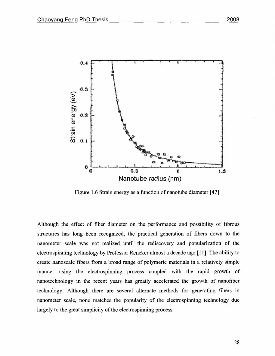
Chaoyanq Feng PhD Thesis 2008
Nanotube radius (nm)
Figure 1.6 Strain energy as a function of nanotube diameter [47]
Although the effect of fiber diameter on the performance and possibility of fibrous
structures has long been recognized, the practical generation of fibers down to the
nanometer scale was not realized until the rediscovery and popularization of the
electrospinning technology by Professor Reneker almost a decade ago [11]. The ability to
create nanoscale fibers from a broad range of polymeric materials in a relatively simple
manner using the electrospinning process coupled with the rapid growth of
nanotechnology in the recent years has greatly accelerated the growth of nanofiber
technology. Although there are several alternate methods for generating fibers in
nanometer scale, none matches the popularity of the electrospinning technology due
largely to the great simplicity of the electrospinning process.
28

Chaoyanq Feng PhD Thesis 2008
2. LITERATURE REVIEW: ELECTROSPINNING OF NANOFIBERS
The technology of electrostatic spinning or electrospinning may be traced back to 1745.
Bose created an aerosol spray by applying a high potential to a liquid at the end of a glass
capillary tube. The principle behind what is now known as electrospinning was furthered
when Lord Rayleigh calculated the maximum amount of charge which a drop of liquid
can hold before the electrical force overcomes the surface tension of the drop [14].
In 1934, Formhals [13] issued a patent for a process capable of producing micron level
monofilament fibers using the electrostatic forces generated in an electrical field for a
variety of polymer solutions. The patent describes how the solutions are passed through
an electrical field formed between electrodes in a thin stream or in the form of droplets in
order to separate them into groups of filaments. This process, later to become known as a
variant of electrospinning, allows the threads, which are repelling each other when placed
in the electric field, to pile up parallel to each other on the filament collector in such a
way that they can be unwound continuously in skeins or ropes of any desired length. The
operational principle of electrospinning is quite simple. In this non-mechanical,
electrostatic technique, a high electric field is generated between a polymer fluid
contained in a spinning dope reservoir with a capillary tip or a spinneret and a metallic
fiber collection ground surface. When the voltage reaches a critical value, the electrical
force overcomes the surface tension of the deformed drop of the suspended polymer
solution formed on the tip of the spinneret, and a jet is produced. The electrically charged
jet undergoes a series of electrically induced bending instabilities during its passage to
the collection surface that results in the hyper-stretching of the jet. This stretching process
is accompanied by the rapid evaporation of the solvent molecules that reduces the
diameter of the jet, in a cone-shaped volume called the "envelope cone". The dry fibers
are accumulated on the surface of the collection plate resulting in a non-woven mesh of
nano to micron diameter fibers. The process can be adjusted to control the fiber diameter
by varying the electric field intensity, collect distance and polymer solution
concentration, whereas the duration of electrospinning controls the thickness of fiber
deposition [13]. A schematic drawing of the electrospinning process is shown in Figure
1.7.
29

Chaoyanq Feng PhD Thesis 2008
and temperature of spinning space, all of these factors will have serious effects on
nanofiber structure and diameter. Further, it will affect the performance of nanofiber
material.
Solution supply syringe
Capillary tip formation of jet
Counter electrode
Polymer Solution
V Nanofiber membrane
High Voltage Power Supplier
ff=-
Schematic diagram of the apparatus of electrospinning
Figure 1.7 Schematic drawing of the electrospinning process showing the formation of
nanofibers under the influence of an electric field
Numerous polymers have been electrospun by an increasing number of researchers
around the world. Examples of some of the polymers that have been successfully spun
are shown in Table 1.2. Solvents and polymers with molecular weights ranging from
10,000 to 300,000 and higher had been electrospun.
Table 1.2 Examples of polymers that have been electrospun
Polymer Nylon 6,6 Polyacrylic acid
Solvent 96 %Formic acid Ethanol
Concentration 12.1 wt%
6wt%
Reference [48] [49]
30

Chaovanq Feng PhD Thesis 2008
Table 1.2 Examples of polymers that have been electrospun
Polymer Nylon 6,6 Polyacrylic acid Polyamide-6 Poly (benzimidazol) Polycarbonate Polyetherimide Poly(ethylene oxide) Mw=400K Poly(ethylene terephthalate) Polystyrene Poly(vinyl alcohol) Poly (vinyl chloride)
Poly(vinyl pyrrolidone) Poly(vinylidene fluoride) Cellulose acetate Collagen Type I Gelatine type A Poly(urethane)
Solvent 96 %Formic acid Ethanol 85 % v/v formic acid Dimethyl acetamide, 185 °C Dichloromethane 1,1,2-Trichloroethane Water
Trifluoroacetic acid
Chloroform Water Tetrahydrofuran: Dimethylformamide = 6:4 Ethanol Dimethylacetamide DMA:Acetone=l:2 Hexafluoropropanol 2,2,2-Trifluorethanol Tetrahydrofuran: Dimethylformamide=6:4
Concentration 12.1 wt%
6wt% 34 wt% 20 wt% 15wt%
14% 10wt%
0.2g/ml
30% (w/v) 25 wt% 13 wt%
4wt% 25 wt% 15wt%
0.083g/ml 10-12.5 wt%
13 wt%
Reference [48] [49] [50] [51] [52] [53] [54]
[55]
[56] [57] [58]
[591 [60] [611 [62] [63] [64]
In addition to the polymers on Table 1.2, many other polymers also have been spun by
electrospinning, including natural biopolymers and inorganic polymers. Polymers were
blended with inorganic compounds to prepare inorganic nano fibers [65]. Hollow
nanofibers were also developed [66].
Electrospinning technology has many advantages such as simple, cheap, and stable. But it
still has many limits: (1) Very low out profits. Typically, its spinning rate is (lmg-lg)/h.
(2) Nanofiber made by electrospinning has a fix structure. It is difficult to spin a single
separated nanofiber. Mostly the product is like non-woven web or mat. (3) There is no
further stretching process. Orientation of macromolecules in the polymer can not be
completed so that nanofibers may not reach expected higher mechanical strength. (4)
Even if numerous papers about nanofiber electrospinning had been published, systematic
research on electrospinning mechanism is still required.
31

Chaovanq Feng PhD Thesis 2008
3. RESEARCH OBJECTIVES
Recently, notable research activities in the field of new membranes for membrane
distillation (MD) are evident in the increased number of patents [67-69] and publications
[70-73]. Generally, research activities are aimed at developing highly hydrophobic or
hydrophobic/hydrophilic composites, and chemically stable membranes. The main results
include the reduction of membrane wetting out, maintaining feasible water fluxes at the
same time. In case of MD for desalination, the selection of membranes has been rather
limited because of the demand for chemical and temperature resistance. As the MD
process for desalination will be operated at a temperature about 80°C, hydrophobic
micro-porous membranes made of polyolefin are not very suitable for such application.
Fluoropolymer materials remain the main group that possesses the required properties to
produce membranes which are suitable for desalination by MD. The most well-known
property for which fluoropolymers are employed in high-demanding applications is their
outstanding thermal and chemical resistance. However, there are yet many challenges to
overcome, which are associated with the use of these materials for membrane
manufacture. The cost of membranes, especially of those that will be used on a large
industrial scale, is a very important issue to be considered as well.
As mentioned, electrospinning technology is suitable to fabricate fibers of high
area/volume ratio and high hydrophobicity. Hence, PVDF, when it is electrospun into
nanofiber, offers a material which is desirable for MD. Even though PVDF is the polymer
of the first choice, other polymers may also be useful to fabricate nanofiber membranes
for membrane distillation.
In the present work, PVDF nanofiber membrane is prepared by electrospinning
technology. The electrospinning conditions are investigated. The PVDF nanofiber
membrane is characterized by SEM, AFM DSC, LEPw, Contact angle analyzer and
mass transfer method. Nanofibers made from other polymers are also investigated. But
the major research work is focused on PVDF nanofiber and PVDF nanofiber membrane
fabrication for desalination by membrane distillation.
32

Chaovanq Feng PhD Thesis 2008
Chapter 2 FABRICATION AND CHARACTERIZATION OF PVDF NANOFIBER AND NANOFIBER MEMBRANE
1. INTRODUCTION
Poly (vinylidene fluoride) is a semi-crystalline polymer that is produced commercially by
a free-radical emulsion or suspension polymerization of vinylidene fluoride (CH2=CF2) in
water [74-76]. PVDF polymer exhibits a unique combination of mechanical and electrical
properties due to the alternating spatial arrangement of CH2 and CF2 groups along the
polymer backbone. PVDF is the fluoropolymer consumed in the greatest quantities aside
from PTFE [77], because of its i) high mechanical and impact strength, ii) resistance to
environmental stress, iii) ease of melt-process ability, and iv) low cost compared to other
fluoropolymers. PVDF is used in architectural coatings (-40%), semiconductor
manufacture and chemical processing (-40%), and wire and cable insulation (-20%)
[78]. A small, but increasing amount of PVDF is used as electrodes in lithium batteries
[79]. Anti-oxygenic property and antipollution property are the most important
advantages of PVDF. Recently, PVDF has been becoming more and more popular
material for membrane fabrication. Its chemical stability is better than other groovy
material, especially for the ability of endurance of washing with oxidizer, since washing
by oxidizer is a main method to solve the fouling problem that ultrafiltration (UF)
membrane may be plugged up by organic matter. Thus, UF membrane made from PVDF
will be more durable, stable and more everlasting. Membranes made from PVDF are
generally chemically inert and, as such, are useful for filtration of a wide variety of fluids.
However, they are not inherently wettable by water. The natural hydrophobicity of PVDF
membranes limits their usefulness in the filtration of aqueous solutions. Different wetting
properties are required for different applications of membranes. Some applications
require wettability by liquids of extremely high surface tensions, while membrane
distillation requires non-wettability by water. In practice, this limitation is a very
important property for membrane distillation. Numbers of researches on membrane
distillation have adopted PVDF membrane [80-85]. PVDF membrane made by phase
inversion or casting and stretching method already has relatively high hydrophobicity. Its
contact angle is higher than 80°, but lower than 90°. Among polymers that have been
33

Chaovanq Feng PhD Thesis 2008
tested for MD, PVDF is considered the best, because of the above mentioned properties.
However, high hydrophobicity would be preferred for desalination by membrane
distillation. Electrospinning nanofiber enhances the hydrophobicity of membrane. Hence
in the present work, it is attempted to use electrospun PVDF nanofiber membranes for
membrane distillation.
2. MATERIALS AND EXPERIMENTAL METHODS
2.1. Materials
Polymers used for electrospinning are as follows:
PVDF, Poly (vinylidene fluoride), (Kynar 761, Elf Atochem)
PES, Polyethersulphone, (ICI, Victrex-4100P)
PS, Polysulphone, (Ultrason®-S, BASF)
PVA, Poly (vinyl alcohol), (Mw -127,000, Sigma-Aldrich)
PEI, Polyetherimide, (Ultem, GE)
PAN, Polyacrylonitrile (Mw 86,200, Sigma-Aldrich)
PC, Polycarbonate, (Mw -20200, Sigma-Aldrich)
PVC, Poly (vinyl chloride), (Mw -62,000, Sigma-Aldrich)
PVP, Poly (vinylpyrrolidone), (K90, Sigma-Aldrich)
Nomex, Polyamide (Dupont)
Collagen-I, (Supplied by Eye Institute of University of Ottawa)
Solvents used for nanofiber electrospinning are as follows:
Chloroform, (CR grade, Sigma-Aldrich)
DMF, Dimethylformamide, (AR grade, Sigma-Aldrich)
DMAc, Dimethyacetamide, (CR grade, Sigma-Aldrich)
HFP: Hexafluoro-2-propanol (Sigma-Aldrich)
IPA: Isopropyl alcohol (Sigma-Aldrich)
Water, Deionized water, (Self-made at lab)
Polystyrene latex: Micro-particles of 0.1, 0.5, 1, 2, 3, 7, 8 and 10 urn in diameter were
34

Chaovanq Feng PhD Thesis 2008
purchased from Sigma-Aldrich (Missouri, USA).
2.2. Nanofiber Preparation by Electrospinning
2.2.1. Preparation of spinning dope
Polymers and solvents used for the preparation of the spinning dopes and the polymer
concentrations are listed in Table 2.1. The polymers cover a wide range of
hydrophilicity/hydrophobicity and the criteria for the choice of the solvent is the high
miscibility of polymer with solvent.
Table 2.1 Polymer, solvent and polymer concentration of the spinning dope
Polymer PVDF
PVDF+PVP PS
PES PEI PVC PC
PAN Nomex (PA)
PVA Collagen
Solvent DMF DMF DMF DMF
DMAc DMF
Chloroform DMF DMF Water HFP
Concentration wt% 20
18+6 18 20 18 10 10 15 15 8
0.12
A 150 mL glass bottle was loaded with polymer and solvent, before it was placed on a
rolling mixer. The mixer was rolled until the polymer was completely dissolved. For the
preparation of the PVA solution, the bottle which contained the polymer and water was
placed in an oven at 90°C and the bottle was shaken manually from time to time until
polymer was completely dissolved and a clear PVA solution was prepared. Even though
various polymers were involved in electrospinning, the major focus material in present
work is PVDF.
It should be emphasized that nanofiber membrane made from polymers other than PVDF
may also be very useful. Nanofiber membranes made of different materials have potential
35

Chaoyanq Feng PhD Thesis 2008
for special applications. For example, Silk fibroin and collagen nanofiber membranes can
be used as a bio scaffold. It may be used for nerve guiding growing, drug release control
or wound dressing [86, 87]. Nanofiber web has already been successfully commercialized
for gas filtration by Donaldson [88]. The filtrate efficiency could reach 99.99% and a
long life was achieved compared with the normal fiber filter. Some new applications have
also been attempted [89]. The use of nanofiber membranes for desalination by membrane
distillation can be considered as one of such exploration of novel applications.
2.2.2. Electrospinning
Electrospinning was conducted by the laboratory made setup illustrated in Figure 1.7.
The polymer solution was supplied by a syringe pump (74900 series, Cole-Parmer). The
volume of the syringe was 10 mL and the flow rate could be adjusted in a range from
0.001 uL/h to 147 mL/min. A needle (27G1/2, BD Pharmingen, San Diego, USA) was
attached to the syringe to be used as the spinneret. The top of the needle was tailored
evenly and was connected to the positive electrode (+) of the high voltage digital power
supply (DW-P503-1C, Tianjin, China) with adjustable voltage (0 to 50 KV) and the
current below 1mA. Aluminium foil used as nanofiber collector was connected to the
negative electrode (-) of the high voltage power supplier. The distance between the top of
the spinneret and the aluminium foil is adjustable within a range of 0 cm to 30 cm. While
electrospinning was conducted, a high voltage electric field was formed in the space
between the spinneret (needle) and the foil. Once the electric force overcame the surface
tension of the polymer solution, nanofiber was spun continuously, until the solution in the
syringe pump was consumed. A membrane is obtained on the aluminium foil in a form of
nonwoven web or mat.
2.3. Membrane Characterization
2.3.1. Optical microscope
Electrospinning process was monitored by an Optical microscope (BH2-UMA,
Olympus). Nanofibers were spun on a glass slide. Under the optical microscope, the fiber
structure was observed. The magnification is adjustable from 20 times to 200 times. The
36

Chaovang Feng PhD Thesis 2008
microscopic image gave the information of the nanofiber such as the approximate
diameter size of nanofiber and the shape of nanofiber. Based on the information,
concentration, voltage and collect distance were adjusted. A more accurate measurement
of the nanofiber diameter was carried out by an Optical microscope (BX40, Olympus)
that could display a digital image of the nanofiber. The measurement of the diameter was
enabled by a scale attached to the digital image. However, due to the limited resolution,
the measurement was not as accurate as the SEM method. Further diameter measurement
was conducted by SEM.
2.3.2. Scanning Electron Microscope (SEM)
Nanofiber samples made from different polymer were prepared by the electrospinng
method described above. The nanofiber was collected on the aluminium foil, before being
cut together with the aluminium foil to 3 x 10 mm without peeling. Then, the aluminium
side of the sample was pasted on a SEM sample holder with a double side carbon
adhesive tape. The sample was put into a sputter-coating chamber to coat with Pt, gold or
carbon. In the present work, the sample was coated with carbon. After sputter-coating the
membrane with a thin carbon film, the sample was mounted on another sample holder
and put into SEM instrument. The morphology was observed by using a Scanning
electron microscope (SEM) (JEOL JMS-6400, Japan).
2.3.3. Contact Angle Measurement
The VCA Optima Surface Analysis System (AST Products, Inc., Billerica, MA) is shown
in Fig. 2.1. It was used for measuring the equilibrium contact angle of nanofiber
membrane made by the above method.
Nanofiber membrane samples were prepared by electrospinning under different
conditions. As for the dense film, it was prepared by using the same polymer solution as
the nanofiber spinning dope. The polymer solution was evenly spread on a glass plate and
placed in a fume hood for 72 hours until solvent was evaporated and a dense film was
formed.
37

Chaoyang Feng PhD Thesis 2008
i»t0:Vo.im,atj*v*Mi\*m.*i*i**:*tviv.ii?fi* : !*«.•.• OKAS
Figure 2.1 VCA Optima Surface Analysis System
Samples prepared for contact angle measurement were evenly placed on a glass slide and
fixed by plastic tape. The sample slide was mounted on the plate holder shown in Fig. 2.1.
The plate can be adjusted by forward or backward, and by left or right movement. Water
drops come from a syringe needle mounted on the top of the sample. The amount of the
water drop can be controlled by a computer system. In the current research, 1 uL water
was fed to form a water droplet. The water droplet was placed on the surface of sample.
Then, the equilibrium contact angle was measured by a digital picture made by a
computer system as shown in Figure 2.1. The equilibrium contact angles were measured
both for the nanofiber membrane and for the dense film.
It should be noted that the collagen nanofiber membrane was cross-linked by
glutaraldehyde. Otherwise, collagen nanofiber membrane dissolves when it comes into
contact with water. Vapour phase cross-linking of collagen nanofiber membrane was
conducted as shown in Figure 2.2. Aqueous glutaraldehyde solution (25 wt% in H2O)
38

Chaoyang Feng PhD Thesis 2008
was loaded in a 50 ml beaker. The beaker with the aqueous glutaraldehyde solution and
the collagen nanofiber membrane were placed in a closed chamber at room temperature
for 48 hours. The size of the chamber is 25x25x30 cm. For safety reason, the chamber
should be kept in a fume hood.
Collagen nanofiber
membrane
25 wt% glutaraldehyde J
Figure 2.2 Vapour crosslinking treatment of Collagen nanofiber membrane
2.3.4. Atomic Force Microscope (AFM)
AFM is a relatively new technology to observe the material structure. It has been
extensively applied on material research and other fields. Compared with SEM, the
sample preparation of AFM is very simple. AFM samples do not need coating or other
pre-treatment. Also AFM images can be obtained at room temperature. It does not need
high voltage and low temperature. The risk of sample damage in the measurement
processing is less than with other methods. The mechanism of AFM is shown in Figure
2.3. A cantilever with a probe is moved under computer control on the top of a sample.
When the probe is close to the sample surface, a repellent force will push the probe away
39

Chaovanq Feng PhD Thesis 2008
from the surface. At the same time, the mechanical spring force of the cantilever will
bring it back to the surface of the sample. As a result, a vibration movement of the
cantilever will occur. The movement is captured by a laser beam, transformed to an
electrical signal which is further transmitted to the detector. Based on the signal, the
computer will give the image of sample surface. In most cases, the sample of AFM is not
coated or treated by pre-treatment. Also the probe will not touch the sample surface.
Therefore, the AFM can bring about more information close to the nature of material.
Laser Diode
Beam Path
Quad
Photo diode
Flexible Cam
Magnetic Disc XYZ piezoelectric
Translator (Scantier)
Sample
Figure 2.3 Mechanism of AFM [90]
Therefore, a nanofiber membrane sample was taped by a double side adhesive tape on a
magnetic metal plate. Then, the plate was mounted on a sample holder. The holder is
controlled by computer to move on 3D axis directions until a clear image was obtained.
As the probe tip of AFM is very fine and sensitive, if membrane has a loose surface, a
particle may comes up and stick on the tip of probe. In this case, clear images, or even no
40

Chaovanq Feng PhD Thesis 2008
images can be obtained.
In the present work, two AFM instruments made by different companies were used. One
AFM system is Nanoscope Digital Ilia from Digital Instruments Inc., Santa Barbara,
USA. The other one is Agilent 5100 AFM/SPM Microscope from Agilent Technologies,
Inc. USA. All AFM images were obtained at room temperature.
2.3.5. Differential Scanning Calorimetry (DSC)
By differential scanning calorimetry (DSC), the thermal properties of a sample are
compared agamst a standard reference material which has no phase transition in
temperature range of interest, such as powdered alumina. Sample and reference are
contained in a small holder within an adiabatic enclosure as illustrated below (Figure 2.4).
Heater 1
Heater 2
Figure 2.4 Schematic diagram of DSC sample holder
The temperature of each holder is monitored by a thermocouple and heat can be supplied
electrically to each holder to keep the temperature of the two equal. A plot of the
difference in energy supplied to the sample against the average temperature, as the latter
41

Chaovang Feng PhD Thesis 2008
difference in energy supplied to the sample against the average temperature, as the latter
is slowly increased through one or more thermal transitions of the sample, yields
important information about the thermal transition. DSC can be used to determine glass
transition temperature (Tg); melt temperature (Tm) and crystallinity of a polymer.
In this research, DSC model QA-1000 (TA Instrument, New Castle, DE, USA) was used.
A nanofiber membrane sample was placed in one of the holders after being weighed. The
sample was then heated from room temperature to 250°C at a heating rate of 10°C/min,
before it was cooled back to -30°C. Another cycle of heating and cooling was then started
from -30°C to 250°C. Two samples were prepared for this experiment. One is a nanofiber
membrane. Another is a dense film cast from the same polymer solution as the spinning
dope. For polymer film preparation, polymer solution was spread evenly on a glass plate
and dried in a fume hood at room temperature for 72 hours until the solvent is completely
evaporated. A small piece of the film was weighed and put in an aluminum case; the
aluminum case was mounted into the DSC-QA 1000 instrument to measure the thermal
behavior of nanofiber membrane and the polymer film.
2.3.6. Liquid Entry Pressure of Water (LEPw)
LEPw is the pressure that must be applied to pure water before it penetrates into dried
membrane pores. This pressure depends on the pore size and the hydrophobicity of the
membrane. The apparatus used for this measurement is shown in Figure 2.5. The
membrane was placed in a static stainless steel cell between the upper chamber (600mL),
the feed side which was filled with pure water, and the lower chamber, the permeate side
which was connected to a digital capillary flow meter (Varian Optiflow 420). First, a
relatively low pressure (3 psi) was applied to the system for at least 10 min; then, the
pressure was increased stepwise with an increment of 0.1 psi. The pressure at which a
continuous flow was observed in the permeate side is the LEPw. This method has been
described extensively by Smolders and Franken [91].
42

Chaovanq Feng PhD Thesis 2008
! t e p i ! a t o r
Air cylinder Figure 2.5 Schematics of the experimental system used for membrane liquid entry
pressure of water (LEPw) measurement
2.3.7. Porosity
Porosity is defined as the volume of the pores divided by the total volume of the
membrane. It can be determined by measuring the density of the polymer material using
isopropyl alcohol (IPA), which penetrates inside the pores of the membrane, and the
density of the membrane using pure water, which does not enter the pores. In this
method, a pycnometer and a balance were employed. The following equation can be used
to determine the porosity as suggested by Smolders and Franken [91].
s = l--^- (2-1) Ppoi
Where, Pm is the density of the membrane and Ppoi is the density of the polymer
43

Chaovang Feng PhD Thesis 2008
material.
2.3.8. Pore size distribution measurement
Molecular-weight cut off (MWCO) of a membrane is defined by IUPAC as the molecular
weight of a solute that gives 90% rejection coefficient [92]. The rejection coefficient is
measured by a filtration experiment and is equal to one minus the ratio of the
concentrations of a component on the downstream side and the upstream side of a
membrane:
Concentration of downstream Rejection coefficient = (1 ) x 100% (2 - 2)
Concentration of upstream
Usually, polyethylene glycol and polyethylene oxide, dextran, cow blood cell and other
molecules are used to measure the MWCO. If the solute molecule had a spherical shape
and the diameter of the spherical molecule could be measured, the diameter of solute
molecule corresponding to the molecular weight cut-off (MWCO) could be used as the
membrane pore size. But in reality, most of the molecular probes to measure the MWCO
are non-spherical, and other methods have to be used.
In the present wok, polystyrene latex micro-particles of 0.1, 0.5, 1, 2, 3, 7, 8 and 10 um in
diameter (Sigma-Aldrich) were used instead of the above mentioned molecular probes.
The latex suspension was reconstituted in distilled water to prepare a 100 ppm suspension
for each particle size. Using these suspensions as feed, separation experiments were
carried out at a pre-set pressure (30 psi) with the wetted PVDF nanofiber membrane. Two
hundred mL of feed was loaded to the feed chamber of the separation cell and the
pressure was applied. The first 5 mL of permeate was discarded to ensure that the steady
state was reached. 30 mL of permeate was collected before the separation experiment was
terminated and the permeation rate was calculated by knowing the time required to
collect 30 mL of permeate. Polystyrene micro-particles concentration in permeate was
determined using the calibration curve. The separation experiment was terminated after
44

Chaovang Feng PhD Thesis 2008
30 mL of permeate was collected. The remaining Polystyrene suspension in the feed
chamber was removed and the cell rinsed three times with distilled water, without
removing the PVDF nanofiber membrane. The solute separation was determined using
the formula below:
/ = ( 1 - 5 L ) X 1 0 0 (2-3)
Where Cp anci Cf a r e m e polystyrene latex suspension concentrations in permeate
collected and the original feed, respectively, which were determined via TOC Analyzer
(Appollo-9000, TELEDYNE Tekmar, Mason, Ohio, USA). / is the solute rejection. It
should be noted that f is basically the same as rejection coefficient defined by equation
(2-2). When solute separation (%) of a membrane is plotted vs. the solute diameter on a
log-normal probability paper, a straight line is yielded [93, 94], which ensures that the
solute separation correlates with the particle diameter according to the log-normal
probability function. Then this relationship can be expressed as:
/ = erf(z) = -L )i^dju (2 - 4)
Where,
27T
z = W ' - ' n ^ ( 2 - 5 )
And ds is the particle diameter, Ms is the geometric mean diameter of the particle and
ag, is the geometric standard deviation about the mean diameter. According to equations
(2-4) and (2-5), a straight line in the form of
45

Chaovang Feng PhD Thesis 2008
F(/) = 4, + 4(ln«/,) (2-6)
will yield between / and ".« on a log-normal probability paper, ^o and A are the
intercept and the slope, respectively. From this log-normal plot, mean particle diameter
(Ms) can be calculated as ds corresponding to / = ^0%. ^g can be determined from the
ratio of " j at J = 84.13 ^ an (j J =50/o Q V ignoring the dependence of solute
separation on the steric and hydrodynamic interaction between the particle and the pore
[93, 94], the mean pore diameter (MP) and the geometric standard deviation (ap)
around the mean pore diameter of the membrane can be considered to be the same as
those of the mean particle size (|4.s) and its geometric standard deviation (as). From
Mp and °P the pore size distribution of a membrane can be expressed by the following
probability density function [95].
df(dp) 1 — = -j= exp
ddp d In <T V2TT
(\ndp-\nnpy
2 ( l n a J 2 . ( 2 - 7 )
where " p is the pore size.
46

Chaovanq Feng PhD Thesis 2008
Chapter 3 RESULTS AND DISCUSSIONS
As mentioned before, electrospinnig technology is a simple and effective method to
fabricate nanometer scale filament material. Within the electrospinnng process,
concentration of the spinning dope, flow rate of the spinning dope, spinning voltage, fiber
collect distance and other factors will affect the diameter of the nanofiber. The effects of
these factors were investigated and the results given below:
1. MORPHOLOGY AND DIAMETER OF NANOFIBER FABRICATED FROM DIFFERENT POLYMERS
The details of the electrospinning conditions are shown in Table 3.1. Spinning was
carried out at room temperature without exception. The optical microscopic and SEM
images of nano fibers spun from different polymers are shown in Fig. 3.1 and Fig. 3.2,
respectively. The images show that fibrous structures were indeed obtained from all the
polymers studied in present research work. However, the nanofiber diameters are quite
different from polymer to polymer, depending on the used polymer and the spinning
conditions. The diameters of nanofiber are based on measuring of images analysis. 25
spots were chosen to calculate an average value of diameter. The standard deviation also
was calculated. The average diameters of the nanofibers are summarized in Table 3.2.
Table 3.1 Electrospinning conditions of nanofibers spun from c
Polymer
PVDF PVDF+PVP (80:20) PS PES PEI PVC PC PAN Nomex (PA) PVA Collagen
Nanofiber collect distance (cm)
18
18
18 18 18 18 18 18 18 18 18
Spinning voltage (kV)
18
18
18 18 18 18 18 18 18 18 18
ifferent polymers Solution feed rate
(ml/h) 2
1
2 2 2 1 1 2 2 1 1
47

Chaovang Feng PhD Thesis 2008
Looking into Fig. 3.2 closely, PES, PS and PEI nanofibers have solid beads. PVC and
Nomex have beads that consist of several smaller beads or nanofibers. Nanofibers made
of PVA and collagen is attached to each other tightly. The shape and morphology of the
nanofiber membrane therefore largely depend on the polymeric material. However, it also
depends on the electro spinning conditions as will be shown for PVDF nanofiber
membranes. More investigations are necessary for the precise control of the nanofiber
morphology.
48

Chaoyang Feng PhD Thesis 2 0 0 8
. ; * ,-*«
' I ! '
PVDF PVDF+PVP
1 • J
PS
t W ^ l u , J _ A » ^ J > -3
PES
1 ^
PEI
1-.
PVC
PC PAN
t i -
Nomex
\ \ . . •
»"«> i>^v
Cottagers
Figure 3.1 Optical microscopic-images of the nanofibers (200 times)

Chaoyang Feng PhD Thesis 2008
t?0NBHKS&? ^
PVDF it
PVDF+PVP
PFS
» • » • * , • • - ^ * * . • »
C * i
FV P V :
Nomex PVA
Coll igtr i
Figure 3.2 SEM images of the nanofibers (5000 times)
50

Chaovanq Feng PhD Thesis 2008
Table 3.2 Average diameter of the nano fibers obtained by image analysis
Polymer
PVDF PVDF+PVP
PS PES PEI PVC PC
PAN Nomex (PA)
PVA Collagen
Nanofiber diameter from optical image (nm)
535±50 433±37 385±32 267±43 250±53 307±61 1396±23 735±45 396±36 325±57
2006±25
Nanofiber diameter from SEM image (nm)
403±32 326±46 290±63 201±52 188±77 231±48 1050±37 553±55 298±67 245±59 1509±66
Note: The average values are based on observations of at least 25 spots.
Although many researchers have reported to fabricate nanofibers by using various
polymers by electrospinning as described in the literature section, investigations were
made on few specific polymers by each researcher. In the present study, 10 polymers and
1 polymer blend are used, covering a wide range of hydrophilicity to hydrophobicity. The
result shows that both hydrophilic and hydrophobic polymer can be electrospun to
nanometer scale filament. But the morphology of nano filament depends on the properties
of polymer, solvent and the spinning condition.
Among others, the diameter of PVDF ranges from 400 to 600 nm. Optical images and
SEM images clearly show that PVDF nanofiber membrane has a fibrous structure.
2. EFFECTS OF ELECTROSPINNING CONDITIONS ON NANOFIBER
DIAMETER
Further investigations were focused on specific polymer (PVDF) nanofiber spinning; the
reason is that PVDF polymer is one of the most hydrophobic polymers among those
51

Chaoyang Feng PhD Thesis 2008
investigated in the present study. As discussed before, the high hydrophobicity is the
most important property required for the membrane to be used in membrane distillation
process.
2.1. Effect of Spinning Voltage
In the present research, the PVDF concentration in DMF solvent and the collect distance
(vertical distance between the top of the syringe needle to the fiber collection plate) were
maintained at 20 wt% and 18 cm, respectively. The dope flow rate was 2 mL/h while the
spinning voltage was changed.
Figure 3.3 shows the optical images of the nanofiber at different spinning voltages, from
which the average nanofiber diameters were obtained. 25 spots were chosen randomly
from the image to measure the diameter of nanofiber. The images show that the fiber
shape depends on the spinning voltage. At low spinning voltage, some beads are
observed and as the voltage increases the beads gradually disappear. However, as the
spinning voltage continues to increase, beads start to appear again.
52
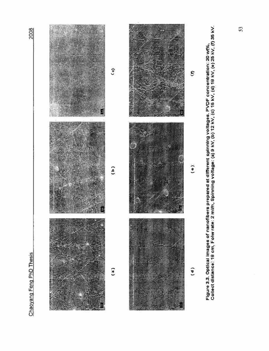
Chao
yang
Feng PhD Thesis
2008
* .
. .-
•
.-.
. •
•-
!
• •.
;
-v
••
•.
•!
. •
• .
: .•
(aj
(b)
(c)
. «
• E
l.
(d
) <
•••)
•:.
<f)
Fig
ure
3.3.
Opt
ical
im
ages
of
nan
ofib
ers
pre
par
ed a
t di
ffer
ent
spin
nin
g vo
ltag
es.
PV
DF
con
cen
trat
ion
: 20
wt%
, C
olle
ct d
ista
nce
: 18
cm
, F
olw
rat
e: 2
mlf
h,-S
pinn
ing
volt
age:
--(a
) 9
kV, (
b) 1
2 kV
, (c
) 15
kV
, (d)
18
kV, (
e) 2
5 kV
, (f)
35
kV.
53

Chaoyanq Feng PhD Thesis 2008
550
g 500 o c ra c u. Q
•S -^ 350
f I
300
250
200
150
100
_y = 0.0372X2 - 5.0306x+ 522.18.
R2 = 0.9366
10 15 20 25 30 35 40
Bectrospinning voltage (KV)
45 50
Figure 3.4 Effect of spinning voltage on nanofiber diameter.
The diameter of PVDF nanofiber is plotted in Fig. 3.4. The diameter decreased with an
increase in spinning voltage. As the spinning voltage increases, the spinning dope that
is extruded in a form of a droplet from the needle (spinneret) tip will have a higher
surface charge density. As a result the electrical potential on the polymer solution
droplet will increase and the electrical force will split the polymer droplet and draw it
from the needle to the low electrical potential side (Aluminium foil: nanofiber
collector). If the applied voltage and the concentration (viscosity) of polymer are high
enough, and the solvent evaporates fast enough, a nanofiber is formed. On the other
hand, if the concentration (viscosity) of the polymer is low, polymer droplets are
sprayed on the collector surface. The later phenomenon has been commercially used
for a long time and is called electro-spray or electrostatic spray. The processing of
electrostatic spray process can be used as an analogy for electrospinning since the
mechanism of both processes are very similar.
54
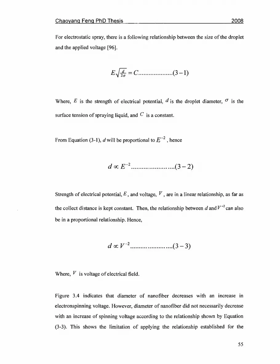
Chaoyang Feng PhD Thesis 2008
For electrostatic spray, there is a following relationship between the size of the droplet
and the applied voltage [96].
E ^ = C (3-1)
Where, E is the strength of electrical potential, d j s the droplet diameter, ° is the
surface tension of spraying liquid, and C is a constant.
From Equation (3-1), d will be proportional to E , hence
docE~2 ( 3 -2 )
Strength of electrical potential, E, and voltage, V s are in a linear relationship, as far as
the collect distance is kept constant. Then, the relationship between d and V~ can also
be in a proportional relationship. Hence,
docV'2 (3-3)
Where, V j s voltage of electrical field.
Figure 3.4 indicates that diameter of nanofiber decreases with an increase in
electronspinning voltage. However, diameter of nanofiber did not necessarily decrease
with an increase of spinning voltage according to the relationship shown by Equation
(3-3). This shows the limitation of applying the relationship established for the
55

Chaovanq Feng PhD Thesis 2008
electrostatic spray to the electrospinning.
Interestingly, however, Nasir et al. [97] showed that diameter of nanofiber was indeed
proportional to V2. In any case, the mechanism of electrospinning has not yet been
established even as much as for the electrospraying process.
2.2. Effect of Spinning Dope Concentration
Electrospinning voltage and collect distance were maintained at 18 kV and 18 cm,
respectively. PVDF concentration in the spinning dope was in a range from 4 to 20
wt%. The flow rate of polymer solution was kept at 2 mL/h. When the PVDF
concentrations were as low as 4 and 6 wt%, nanofibers were very hard to be obtained.
The reason is when the viscosity of the solution is very low. Since the liquid fibers
travel through the collect distance very fast, the solvent is not removed completely
when they reach the collect plate. The fibers merge on the collect plate without
producing any solid fibers.
Fig. 3.5 shows the optical images of the electrospun nanofibers. Even though good
nanofibers were obtained when the PVDF concentration was equal to or above 8 wt%,
with few or no beads found on the formed nanofibers, the diameter of the nanofiber
filament is un-even along the fiber axis, when the concentration of PVDF in the
spinning dope was lower than 16%.
56

Cha
oyan
g F
eng
PhD
The
sis
2008
(*•>
:•
(b
) C
c)
^
(d )
(
e)
CO
Fig
ure
3.5
Th
e o
pti
cal
ima
ge
s o
f n
an
ofi
be
r p
rep
are
d fr
om
dif
fere
nt
po
lym
er
con
cen
tra
tio
n.,
Flo
w r
ate
: 2
ml/
h,
Co
llect
dis
tan
ce:
18 c
m,
Sp
inn
ing
volt
ag
e:
18 K
V P
VD
F c
on
cen
tra
tio
n:
(a)
8 w
t%,
(b)
12 w
t%,
(c)
14
wtP
/o, (
d) 1
6 w
t%,
(e)
18 w
t%,
(f)
20
wt%
.
57

Chaovang Feng PhD Thesis 2008
The relationship between the concentration of PVDF in the spinning dope and the
diameter of PVDF nanofiber is shown in Figure 3.6. Similar trends were also observed
by Nasir et al. [97]. With an increase of PVDF concentration in the spinning dope, the
diameter of PVDF nanofiber increases. As the polymer concentration of the spinning
dope increases, the viscosity of the dope will increase and the surface tension of the
spinning dope will also increase. A higher force is required to draw the polymer
solution out from the spinneret (needle) and the spray stream will also have less
chance to split.
Figure 3.6 Effect of spinning dope concentration on nanofiber diameter.
Deitzel et al. studied the electrospinning of polyethylene oxide (PEOyFbO solutions
and found the following relationship between the diameter of PEO nanofiber and the
PEO concentration of spinning [22].
J o c c 0 5 ( 3 - 4 )
Where, d is the diameter of the PEO nanofiber and C is the PEO concentration of the
58

Chaovanq Feng PhD Thesis 2008
spinning dopes.
Baumgarten used the PAN/DMAc solutions to electrospin PAN nanofibers [98]. He
found that the diameter of PAN nanofiber and the viscosity of the spinning were
related to each other by the following equation.
doer?05 (3-5)
Where, d is the diameter of the PAN nanofiber and V is the viscosity of the spinning
dope.
For both equations, increasing in nanofiber diameter with an increase in the
concentration of polymer solution can be predicted. Indeed, the results shown in Fig.
3.6 exhibited the predicted trend, but the fiber diameter was not necessarily
proportional to either the square root of the concentration or the square root of the
dope solution viscosity. Because Equations (3-4) and (3-5) are empirical equations for
a specific polymer and electro-spray condition, they are not universal equations for
nanofiber spinning. The theoretical research of nanofiber spinning by electrospinning
technology is still at the initial stage.
For fiber spinning, the viscosity of spinning dope is more important than the
concentration since viscosity is related to rheological behaviour of solution. For the
polymer solution, viscosity is related to concentration, and in most cases the
relationship is not linear.
The following equation is one of such relationships.
59

Chaovanq Feng PhD Thesis 2008
f \d-2*)
^ o = 1 + (l - 2k)x c x [77J (3 - 6)
Where, k is the Huggins-Martin constant, [n] is the intrinsic viscosity, c is the
concentration of polymer solution, no is the viscosity of the solvent [99].
Another interesting thing to be studied is the effect of temperature on the nanofiber
diameter. In a limited range the relationship between the viscosity of the polymer
solution and the temperature is given by Andrade's viscosity equation [99]:
r] = Dem (3-7)
Where *7 denotes the viscosity, T the temperature and D and B denote empirical
coefficients that can be determined by experiments.
Usually B has a negative value and the viscosity decreases with an increase in the
temperature. Combining equations (3-5) and (3-7), a decrease in the nanofiber
diameter is predicted with an increase in the temperature. This however was not
confirmed by the experiment due to the limitation in available equipment.
Optical images in Fig. 3.5 shows that fine nanofibers can be obtained at PVDF
concentrations equal to or above 8 wt%. It is difficult to conclude from Fig. 3.5 alone
which dope concentration is the best. For the present research, 20 wt% was chosen
arbitrarily for nanofiber membrane fabrication.
2.3. Effect of Collect Distance on Nanofiber Diameter
The electrospinning voltage and the PVDF concentration of the dope solution were
maintained at 18 kV and 20 wt%, respectively. The flow rate of polymer solution was
60

Chaovanq Feng PhD Thesis 2008
maintained at 2 mL/h. Only the nanofiber collect distance was changed. The optical
images are shown in Fig. 3.7, and experiment results are summarized in Fig. 3.8.
In Fig. 3.7, the optical images indicate that with the collect distance increasing, the
nanofiber shape changed from without beads to with beads.
The electric field surrounding a point charge is given by Coulomb's law:
E = -?-%? (3-8) 4n;e0 r
Where, Q is the charge of the particle creating the electric field, r is the distance from
the particle with charge Q to the electric field evaluation point, r is the Unit vector
pointing from the particle with charge Q to the electric field evaluation point, £o is the
vacuum permittivity.
Coulomb's law is actually a special case of Gauss's law, a more fundamental
description of the relationship between the distribution of electric charge in the space
and the resulting electric field.
According to Equation (3-8), as the collect distance increases, the intensity of
electrical field will decrease; i.e. the electrical force decreases. As the force for
electrospinning decreases, more beads are formed.
61

Chao
yang
Feng PhD Thesis
2008
• 4
'
i •
7 •
;'
' •
•.•
••
V
V
(d)
( e
)
(a)
(b)
. > .
.'
<c)
Fig
ure
3.7
Th
e o
pti
cal
imag
es o
f n
ano
fib
er p
rep
ared
wit
h d
iffe
ren
t co
llec
t d
ista
nce
s P
VD
F c
on
cen
trat
ion
: 2
0 w
J%
, Sp
inn
ing
vo
ltag
e: 1
8 K
V,
Flo
w r
ate:
2 m
l/h
, C
oll
ect
dis
tan
ce
: (a
) 12
cm
, (
b)
15
cm,
(c)
18 c
m, (
d)2
1 c
m,
(e)
24
cm
.
62

Chaoyang Feng PhD Thesis 2008
According to Fig. 3.8 the diameter of the PVDF nanofiber slightly decreases as the
collect distance increases. Thus, the increase in collect distance will help to obtain
finer nanofibers.
(J-,
> Cu
<w
o *H CD
4-> CD
(VI •r-I
-ct CD bn cO U CD
> •<
^
nra
• - — '
u CD
•i-H
4H
o a c
600 550 500
450 400
350 300 V,h(l 200
ISO 100
50 0
0. 3444x' - 19. 02x + 702. R2 = 0.8819
10 12 14 16 18 20 22 24 26 Distance between spinning needle and collector (cm)
Figure 3.8 Effect of collect distance on nanofiber diameter
The collect distance is an important parameter for nanofiber electrospinning and it also
needs to be properly controlled. A long collect distance enhances solvent evaporation
along the way from the spinneret to the collect plate and the polymer solidification
becomes more complete. This means that nanofibers do not stick to each other.
Nanofiber membrane structure becomes loose.
To fabricate individual nanofibers is another very important research direction for
nanofiber and nanofiber membrane. For example, nano-carbon tube is a filament
structure material with diameter less than lOOnm. By Template, Vapour Grown,
Molecular Assembly and other methods, single carbon nanotube can be prepared. But
the length of carbon nanotube is limited when prepared by the above methods. By
improving the collect method for electrospinning, single or individual polyacrylonitrile
63

Chaovanq Feng PhD Thesis 2008
(PAN) nanofibers can be prepared and they can be used as the precursor of carbon
nanofibers. According to the definition of nanotube, if the diameter of carbon
nanofiber is less than lOOnm, it is exactly carbon nanotube. This kind of carbon
nanotube is very useful for hydrogen storage, super large capacitor, fuel cell and
electron device. Hence, electrospinning is a new and practical approach for many
potential applications.
Even though for other applications of nanofibers, the separation of each fiber is more
favourable, for membrane applications, nanofibers should stick to each other to some
extent, to maintain the membrane integrity and to enhance the mechanical strength of
the membrane. Since the nanofiber attachment depends on the collect distance for the
above mentioned reasons, the collect distance needs to be properly controlled. If the
collect distance is too short, the attachment will be excessive, while, if the distance is
too long, the fibers will be separated. For this reason, an intermediate value of 18 cm
was chosen to be used hereafter. However, it should be admitted that this is a quite
arbitrary choice.
2.4. Effect of Polymer Solution Flow Rate
In the present research, the spinning voltage and PVDF concentration in the spinning
dope were maintained at 18 kV and 20 wt%, respectively. Collect distance was set
equal to 18 cm. The only parameter changed was the flow rate of the dope solution.
Optical images (Fig. 3.9) show the change of the diameter of PVDF nanofibers with
the change of the dope flow rate. With the increasing in dope flow rate, the diameter of
the PVDF nanofiber seems to increase slightly. In order to enable continuous
nanofiber spinning, the dope flow rate should be above a limiting value that allows a
sufficient amount of the spinning dope to be extruded.
It should be noted that 6 mL of the spinning dope was required for spinning,
64

Chaovang Feng PhD Thesis 2008
particularly to obtain a sufficient membrane area and thickness on the aluminum foil.
The mat together with the aluminum foil was dried in a fume hood for 48 hours. Then,
the nanofiber membrane was carefully peeled off from the aluminium foil prior to its
use as a nanofiber membrane for characterization study and for membrane distillation
study.
65

Chaoyanq Feng PhD Thesis
2008
••'•
••':
>c^
i"!^
- .
-.
• '
.''•
-•
'.*
':"?
•".•
•:,!
. '-
•
.V'.
•
"'
•
.•
Wff
'• —
H
-
- U
kJL.
'^L.
' V
<^
^
fa)
(b
) C
c)
Fig
ure
3.9
Th
e o
pti
cal
ima
ge
s o
f P
VD
F n
an
ofi
be
rs p
rep
are
d w
ith
dif
fere
nt
flo
w r
ate
s.
Sp
inn
ing
volt
ag
e:
18 k
V,
PV
DF
co
nce
ntr
ati
on
: 2
0 w
i%, C
olle
ct d
ista
nce
18
cm
, F
low
ra
te:
(a)
2 m
l/h
, (b
)4 m
l/h
, (c
) 8
ml/
h,
(d)
16 m
l/h
, (e
) 3
2 m
l/h
, (f
) 64
ml/
h.
4m
(.*•)
(
e)
CO
^Jl^
fflL
j 66

Chaoyang Feng PhD Thesis 2008
The effect of polymer solution flow rate on the average diameter is summarized in Fig.
3.10.
700
E 600
.Q
o c co c
LL. Q > 0.
500
400
2 300 + J V E .2 200 •o <u o> 2
100 > <
0 1 2 3 4 5 6 7 8 9 10111213141516171819202122232425262728293031323334
Flow rate of polymer solution (mL/h)
Figure 3.10 Effect of polymer solution flow rate on nanofiber diameter
Figure 3.10 shows that the diameter of PVDF nanofiber slightly increases with increasing
spinning dope flow rate. Polymer solution comes out from the spinning needle with an
electric charge. When the spinning dope flow rate increases, the amount of the electric
charge increases, hence the electric field intensity also increases. But the increase in the
charge amount eventually levels off; dope flow rate can continue to increase. Due to the
decrease in charge density, there is less chance for nanofiber to split. This is the reason
for the slight increase of fiber diameter with an increase in flow rate of polymer solution.
The process is shown as in Fig. 3.11.
67

Chaoyanq Feng PhD Thesis 2008
Low flow rate High flow rate (Positive, +)
Spinneret needle
Polymer solution droplet ^ f ? - . . D
Collect plate
(Negative, -)
Figure 3.11 Effect of polymer solution flow rate on nanofiber spinning
3. PVDF NANOFIBER MEMBRANE CHARACTERIZATION
3.1. Scanning Electron Microscope (SEM)
Figure 3.12 shows the SEM images of PVDF nanofiber membranes obtained under the
following conditions; spinning voltage 18 kV, polymer concentration in the dope 20 wt%,
collect distance 18 cm and polymer solution flow rate 2 mL/h.
68

Chaoyanq Feng PhD Thesis 2008
SEM of PVDF nanofiber membrane (X5000)
Figure 3.12 SEM of nanofiber membranes
According to the SEM images shown in Fig. 3.12, the membrane was formed by random
arrangement of nanofibers. Considering the spaces between the nanofibers as pores, the
size of the pores of this membrane are several micrometers. The pore size, together with
the high hdrophobicity of the PVDF membrane, makes the PVDF membrane appropriate
to be used for membrane distillation.
It should be noted that unlike many membranes made by the phase inversion or other
methods, the PVDF nanofiber membrane consists of open pores, which means the pores
are interconnected. It is expected therefore that the vapour can easily and freely pass
through the nanofiber membrane in membrane distillation. Further detailed analysis of
accurate pore size and pore size distribution was conducted by particle separation
experiments. However, the SEM images give a clear idea that nanofiber membrane has a
completely different structure when compared with membranes fabricated by the phase
inversion and other methods.
Figure 3.13 shows the SEM of nanofiber made from different polymers, spun under the
conditions reported in Table 3.1. Although nanofibers could be spun under the given
conditions the morphology of nanofiber is different, depending on the polymer. Similar
trends are observed as those discussed in section 1 of this chapter.
SEM of PVDF nanofiber membrane (X10000)
69

Chaoyang Feng PhD Thesis 2008
PVDF+PVP
it .
e -« i i * »-
PS
PES PEI
•fSWtrH
•,-•> * / • • ' . ' • • • ' ;>-..--V.»v-».'v \ b ' . < • » ' , . ; , ' ' i - >
PVC PC
70

Chaovanq Feng PhD Thesis 2008
PAN Nomex (PA)
PVA Collagen
Figure 3.13 SEM images of nanofiber membrane made from different polymers
3.2. Atomic Force Microscopy (AFM)
AFM is a relatively new technology to observe the material structure. It has been
extensively applied in material research and other fields. AFM has also been extensively
used to observe the membrane surface morphology [90]. Compared with SEM,
preparation of the AFM sample is simple, since sample coating or other sample pre-
treatments are not necessary. For this reason, AFM image will release more information
close to the nature of materials. Also it does not need high voltage and low temperature.
The risk of sample damage is therefore less than other methods such as SEM. However,
to observe nanofiber membranes by using AFM needs a special skill. Since the
71

Chaoyang Feng PhD Thesis 2008
nanofibers are only randomly and loosely attached to each other, a fibre can be adhered to
the cantilever tip and move together with the cantilever tip, which makes the response of
the cantilever tip to the surface structure inaccurate. In this case, the image becomes
either unclear or even no image is obtained.
AFM images are shown in Figs. 3.14 to 3.16 for PVDF and PES nanofiber membranes.
5.00
2.SO
2.4 UM
1.2 UM
'0.0 UM
NanoScope Scan size Setpoint Scan rate NuMber of sawples
TMJ»FH 5.000 UM S.413 W 2.001
2S6 Hz
UM
Figure 3.14 AFM image of PVDF nanofiber membrane (Digital III)
72

^haovang Feng PhD Thesis
Figure 3.15 AFM images of PVDF nanofiber membrane (Molecular Image)
wsjBao ajjaggssgupgoikagiaia aaapoj; -•.
F=T=f=r=j
.aJEUiJl i| - W3gjMS>m>^<3m?(&£^oarit&:i)i^
=^T=^
JSJ.*i
Figure 3.16 AFM images of PES nanofiber membrane (Molecular Image)
73

Chaovanq Feng PhD Thesis 2008
Similar to the SEM images, the AFM images also show the random arrangement of
nanofibers. However, more details of the fibre surfaces can be observed by AFM.
Interestingly, even though the images shown in Figs. 3.15 and 3.16 are for the nanofiber
membranes made of different polymeric materials, the essential feature of the surface
morphology is similar; i.e. aggregates of macromolecules are aligned vertically to the
axial direction of the fiber. This surface morphology was observed for the first time by
the present work.
The formation of the observed nanofiber morphology is explained in the following way.
As a dope droplet is extruded from the spinneret, it is split into a very fine polymer
solution stream by the electrical force. Along the way from the spinneret to the collector,
solvent evaporates and the polymer solidifies. The polymer aggregates are packed closely
due to the capillary force working between the aggregates as the solvent evaporates very
fast from the surface. It is well known that the polymer aggregates are closely packed at
the top surface of the dense membrane. As the distance from the surface increases, the
packing density decreases. It is interesting to note that only the densely packed layer is
observed in the nanofiber because the diameter of the fiber is in the nanometer range.
This structure suggests an extremely high mechanical strength of a single nanofiber since
there is hardly any defects observed in the densely packed layers of polymer aggregates.
Indirect evidence is found in the literature [46], where it is reported that the strength of
glass fiber increases dramatically, with a decrease in the diameter.
It is also speculated that if a two dimensional film of a similar structure (a single layer of
closely packed polymer aggregates) obtained instead of one dimensional nanofibers, it
could be used as air filter of extremely high selectivity, and also permeability. The
company named Donaldson had used nanofiber nonwoven mat as air filter and it reached
99.99% separation. [88]
The AFM of the PES nanofiber membrane also shows clearly that many nanofibers are in
contact with other fibers, while in the PVDF naofiber membrane, the nanofibers are more
separate from each other. It seems that the degree of contact of the fibers depends on how
74

Chaovanq Feng PhD Thesis 2008
completely the solvent is removed while the nanofiber is travelling from the spinneret to
the collector. The more the residual solvent remains in the nanofibers, the more contact
points are formed among the nanofibers. This is favourable for having strong mechanical
strength for the nanofiber membrane. One the other hand, as the degree of contacts
decreases the porosity becomes higher; the membrane becomes looser, resulting in an
increase in the membrane's permeability.
3.3. DSC of Nanofiber Membrane
Differential scanning calorimetry is a widely used technique to study the thermal
properties of polymer. In particular, the technique is applied to study the thermal
transitions of a polymer. Thermal transitions are defined as the changes that take place in
a polymer when the polymer is heated.
ExoUp 100
Temperature (°C) 250
Universal V4.2E
Figure 3.17 DSC results of PVDF nanofiber membrane and dense PVDF film
PVDF has a glass transition temperature (Tg) of about -35°C and melt temperature (Tm)
of about 168 °C (Elf AutoChem). Since the temperature range of this experiment was
75

Chaovanq Feng PhD Thesis , 2008
from -30 °C to 250 °C, the glass transition of PVDF could not be detected. Therefore,
only Tm results are shown in Fig. 3.17.
In Fig. 3.17, for the PVDF film, the Tm was 159.47 °C and 160.73 °C for first heating and
second heating, respectively. But for the PVDF nanofiber membrane, the Tm was 153.17
°C and 156.34 °C for the first heating and second heating, respectively. It reflects the
structural change of the polymer after electrospinning. As the size of materials goes down
to the nanometer range, each independent part of the materials becomes aggregates of
few molecules to few hundred molecules. The affinity between the separate parts will be
less than affinity between molecules themselves. Therefore, the Tm of PVDF polymer
deceases from the film to the nanofiber. It is another evidence for the nanonization of
PVDF material by electrospinning. Similar results were reported by Choi and co
workers [100].
Similar DSC results have been obtained from the PES polymer. But in PES, the glass
transition temperature (Tg) was obtained instead of the polymer melting point. For PES
the glass transition temperature (Tg) is reported to be 230 °C [101].
Figure 3.18 shows that Tg values of the PES film were 213.76 °C and 214.07 °C,
respectively, for the first and second heating. On the other hand, those of the PES
nanofiber were 199.27 °C and 206.74 °C, respectively. After nanonization of PES, the Tg
of the polymer decreased. This also indicates the change in the degree of crystallinity.
76

Chaovang Feng PhD Thesis 2008
Exo Up 50 100
Temperature (°C) 200 250
Universal V4.2E
Figure 3.18 DSC of PES nanofiber membrane and PES dense film
3.4. Contact Angle of Nanofiber Membrane
The contact angle is the angle at which a liquid/vapour interface meets the solid surface
(Fig. 3.19). The contact angle is specific for any given system and is determined by the
interactions across the three interfaces. Most often the concept is illustrated with a small
liquid droplet resting on a flat horizontal solid surface. The shape of the droplet is
determined by the following Young-Laplace equation [102]. Contact angle is measured
using a contact angle goniometry.
yLV cos<9 = y s v -ySL (3 -9)
Where, Y LV , Ysv and YsL TQ^er t 0 m e hiterfacial tension of the liquid/vapour,
solid/vapour and solid/liquid interfaces, U is the contact angle.
77

Chaoyang Feng PhD Thesis 2008
VAPOR - / ^ — - —
LIQUID Ysv y n YSL
SOLID
Figure 3.19 Contact angle of solid material
Consider a liquid droplet on a solid surface. If the liquid is very strongly attracted to the
solid surface (for example water on a strongly hydrophilic solid) the droplet will
completely spread out on the solid surface and the contact angle will be close to 0°. Less
strongly hydrophilic solid surface will have a contact angle up to 90°. If the solid surface
is hydrophobic, the contact angle will be larger than 90°. On highly hydrophobic
surfaces, the surfaces have water contact angles as high as 150° or even nearly equal to
180°. On these surfaces, water droplets simply rest on the surface, without actually
wetting to any significant extent. These surfaces are termed superhydrophobic and can
be obtained on fluorinated surfaces (Teflon-like coatings) that have been appropriately
micro patterned. This is called the Lotus effect, as these new surfaces are based on lotus
plants' surface (which has little protuberances) and would be super hydrophobic. The
contact angle thus directly provides information on the interaction energy between the
surface and the liquid.
As discussed earlier, a membrane suitable for desalination by membrane distillation is
required to have high hydrophobicity. Hence, the contact angle is an important property
of the membrane and it needs to be carefully investigated.
Figure 3.20 shows the digital picture of water droplet on PVDF nanofiber membrane, and
Fig 3.20 (A) shows the method of contact angle measurement. Fig. 3.20 (B) shows the
digital picture of water rest on the surface of a PVDF nanofiber membrane.
78

Chaovang Feng PhD Thesis 2008
/
(A) (B) Contact angle of PVDF nanofiber membrane Water droplet on the surface of
PVDF nanofiber membrane
Figure 3.20 Contact angle measurement
Table 3.3 summarizes the equilibrium contact angles of PVDF nanofiber membranes
which were made at different spinning conditions.
Table 3.3 Contact angles of PVDF nanofiber membranes
Nanofiber membranes
PVDF inDMF
Electrospinning conditions
Distance (cm)
Voltage (kV)
Flow Rate (ml/h)
12
15 18 21 24 15 20 25 30 35 2 4 8 16 32
Equilibrium Contact angle (°)
118 ±3
123 ±5 119 ±2 115 ±4 122 ±5 124 ±3 116 ±5 123 ±3 119 ±4 118±5 119 ±2 118 ±4 122 ±2 116 ±3 119 ±3
Note: PVDF polymer solution concentration: 20 wt%
79

Chaovanq Feng PhD Thesis 2008
It shows that the average equilibrium contact angles of PVDF nanofiber membranes were
distributed randomly around a value of 119°. It can be concluded that the electrospinning
condition has less effect on contact angle of PVDF nanofiber membrane. Together with
the data shown in chapter 3 section 3.2, it can also be concluded that when the diameter
of nanofiber reaches nanometer range, the fiber diameter does not affect the contact angle
of nanofiber membrane.
The equilibrium contact angles for the nanofiber membranes made from different
polymers under the conditions specified in Table 3.1 were also measured and the results
shown in Fig. 3.21.
Figure 3.21 Equilibrium contact angle of nanofiber membranes and dense films made
from different polymers. 1) Blue bar: contact angle of polymer film.2) Brown bar:
contact angle of nanofiber membrane
Figure 3.21 shows the equilibrium contact angle of nanofiber membranes made from
PVDF, PVDF blended with PVP, PS, PES, PEI, PVC, PC and PAN increased
dramatically from the contact angle of the dense film up to above 119°. However, contact
angles of the nanofiber membranes made from hydrophilic polymers such as PVA and
collagen did not increase very much.
80

Chaovanq Feng PhD Thesis 2008
From Fig. 3.21, there seems to be a threshold value of 35° of the dense film. Below the
threshold value the contact angle of the nanofiber membrane does not increase very
much, although some increase is noticed. Above the threshold value, a sharp increase in
the contact angle is observed. Therefore, it can be concluded that the contact angle
depends not only on the chemical property but also on the physical structure of the
sample. Recognizing the effect of the physical structure of the sample, some researchers
developed a superhydrophobic surface of nanofiber structure from hydrophilic polymer
by template method. According to this report, the contact angle even reached 173° [32].
It has been known that contact angle is seriously affected by the porous structure of the
material. The reason for these phenomena could possibly be obtained from the lotus
effect and from Cassie's law [103]. Cassie's law describes the effective contact angle 9C
for a liquid on a composite surface. The law explains how the increase in roughness of a
surface increases the apparent contact angle. The law is stated as:
cos#c = yx cos#j +y2 cos#2 (3-10)
Where 6\ is the contact angle for component 1 with a fraction Y\ and $2 is the contact
angle for component 2 with a fraction Yi present in the composite materials. This
equation takes on special meaning when in a 2-component system one component is air
with a contact angle of 180°. As COS(180) = - 1 , the equation reduces to:
cos^fifcostfj+l)-! (3-11)
Since yi+ Y2 = 1. Equation (3-11) implies that with a small Y\ and a large &x 5 it is possible
to create surfaces with a very large contact angle. For example, the above equation points
out that the water repelling quality of ducks is due to the very nature of the composite
formed between air and feather and not by other causes such as the presence of
exceptional proofing agents like oils. Water striders also exploit this phenomenon.
81

Chaovanq Feng PhD Thesis 2008
Artificial superhydrophobic materials such as nanopin film in the laboratory also
make use of this law. The lotus effect in material science is the observed self-cleaning
property found with lotus leaves. Their microscopic structure and surface chemistry of
lotus leaves mean that the leaves never get wet. Rather, water droplets roll off a leafs
surface like mercury.
In the present work, most nanofiber membranes made from different polymeric materials
exhibited very high contact angles. These results could be explained by the images of
AFM, SEM and from Cassie's law. The nanofiber membranes have composite structures
where single nanofibers are laid down in random way. The spaces among nanofibers are
filled with air. The difference between the structure of the nanofiber membrane and that
of the lotus leaf is possibly in the fact that nanofibers in the nanofiber membrane are
arranged horizontal to the surface, while in the lotus leave they are vertical to the surface.
That means a water droplet has a chance to contact with a larger area of nanofibers. This
may be the reason why the contact angle of the nanofiber membrane is smaller than that
of the lotus leaf. The super-hydrophobic surface developed from a hydrophilic polymer
provides another evidence for this theory [32].
For many different polymers, their nanofiber membranes have large contact angles.
Theoretically, they may have the potential to be used for membrane distillation for
desalination. But the MD membrane requires permanent hydrophobicity. Therefore, in
this study, PVDF was chosen as the target material for further investigation for MD.
Figure 3.22 is digital pictures of equilibrium contact angle of those nanofiber membranes
measured by VCA Optima Surface Analysis System. It clearly shows the PVDF
nanofiber membrane has a high contact angle. Naonifiber membranes made from PS,
PES, PEI, PC and PVC polymers also have very high contact angles. Compared with
other polymers used in this study, PVDF seems to have one of the highest intrinsic
hydrophobicities. For this reason, PVDF nanofiber membrane was chosen for further
study.
82

Chaovang Feng PhD Thesis 2008
PVDF PVDF+PVP
PS
PEI
PES
tttm
PVC
PC
Nomex (PA)
PAN
PVA
Collagen
Figure 3.22 Digital pictures of contact angle measurement
3.5 Porosity of Nanofiber Membrane
83

Chaoyang Feng PhD Thesis 2008
The porosity of a porous medium describes the fraction of void space in the material,
where the void may contain, for example, air or water. It is defined by the ratio:
K .(3-12)
Where, & is the porosity of material, *v is the volume of void-space (such as fluids) and
VT is the total or bulk volume of material, including the solid and void components.
Porosity is a fraction between 0 and 1, typically ranging from less than 0.01 for solid
granite to more than 0.5 for peat and clay.
The porosity of membrane is an important parameter to describe the membrane property
particularly when the membrane is applied for membrane distillation, since it will decide
the transport of the vapour through membrane. Porosities obtained by experiments are
summarized in Table 3.4.
Table 3.4 Porosity of nanofiber membranes made from different polymers
Nanofiber membrane PVDF
PS PES PEI PVC PC
PAN Nomex (PA)
PVA Collagen
Membrane porosity (%) 76±5 72±6 78±2 69±4 66±3 58±5 67±7 63±4 51±3 46±2
Table 3.4 indicates that the porosity decreases as the hydrophobicity of the polymer
decreases. This may also be the reason why the contact angles of the nanofiber
membranes were not significantly higher than those of the dense films for the hydrophilic
polymeric materials. The amount of air contained in the nanofiber membranes made of
polymers of low hydrophobicity was not as high as in the nanofiber membranes made of
highly hydrophobic material.
84
Chaovanq Feng PhD Thesis 2008
Porosities reported in Table 3.4 are not necessarily higher than the commercially
available microfiltration membranes that are currently used for membrane distillation. In
most cases, the porosity of commercially available membranes used for membrane
distillation is in a range 0.7-0.8 [104]. Only the membranes made from the three highest
hydrophobic polymers (PVDF, PS and PES) reached the range of commercial
membranes. However, as mentioned earlier, the nanofiber membrane has, unlike the
membranes made by the phase inversion and stretching technique, an open pore structure,
which enables the vapour transport from one pore to the other. This will enhance the
vapour permeability through the membrane. PVDF nanofiber membranes have the
highest porosity and open pore structure, which is also the reason why PVDF was chosen
for membrane distillation experiments.
3.6. Liquid Entry Pressure of Water (LEPw)
The separation process known as membrane distillation (MD) usually refers to the
thermally driven transport of vapour through micro pores of hydrophobic membranes.
The liquid feed is always in contact with the membrane and can not penetrate into dry
membrane pores unless a transmembrane hydrostatic pressure that exceeds the so-called
liquid entry pressure of water (LEPw) is applied [104-110]. When, the hydrostatic
pressure is lower than the LEPw, the feed liquid does not enter the pores, and a liquid-
vapour interface is formed at the entrance of each membrane pore. LEPw above 3 psi is
normally considered as sufficient to hold the liquid outside of the membrane pore. This
value is required since the pressure at the feed inlet is not necessarily atmospheric
pressure, even when the feed outlet is kept at atmospheric pressure due to the pressure
drop from the inlet to the outlet of the feed. Hence, to hold the feed liquid outside of the
membrane pore, a certain LEPw is required.
The LEPw values of nonofiber membranes made of different polymeric materials are
summarized in Table 3.5.
Interestingly, the data shown in Table 3.5 do not show any trend between LEPw and
hydrophobicity/hydrophilicity. The reason may be that the LEPw is determined by the
interplay of hydrophobicity and pore size.
85

Chaoyang Feng PhD Thesis 2008
Table 3.5 LEPw of nonofiber membranes made from different polymeric materials Nanofiber membrane
PVDF PS
PES PEI
PVC PC
PAN
LEPw (psi) 17.6±2 23.2±1 18.6±3 21.4±1 27.0±2 19.2±4 27.6±1
3.7. Pore Size and Pore Size Distribution of Nanofiber Membrane
Figure 3.23 shows the solute separation versus Polystyrene latex particle diameter for the
PVDF nanofiber membrane and for the PVDF/PVP blend membrane. The
electrospinning conditions are specified in the caption.
From Fig. 3.23 and the definition of MWCO [92], the MWCO of the PVDF and the
PVDF/PVP blend nanofiber membranes are 1.38 um and 2.51 jam, respectively, in terms
of particle size (not molecular weight).
100
.90
"JJ 60
= TQ
'•£ 60
3 50
^-~* . J l ^ _ _ _ _ ., 0 - --— - i
/!X! / * ' J* i
/ / i i
—*—Membrane- I
-®—Membrane II
// i i # — « 7 t
.1 ', , » i , , , , , , I,
2 3 4 5 6 7 8 9
Polystyrene l a tex p a r t i c a l s ize (̂ uii) 10
Figure 3.23 Solute separation vs. Polystyrene particle diameter obtained by filtration experiments I) PVDF concentration 20%, spinning voltage 18kV, collect distance 18cm, dope flow rate 2mL/h. II) PVDF+PVP concentration 20%, spinning voltage 18kV, collect distance 18cm, dope flow rate 2mL/h. Filtration experiments were performed at 30 psig and latex concentration of 100 ppm.
86

Chaoyang Feng PhD Thesis 2008
(2
PVDF nanoflber pore size, d (mm)
100
Figure 3.24 Log-normal probability plot of solute separation vs. Polystyrene particle size
Membrane preparation and filtration experimental conditions, same as Fig. 3.23
Membrane I
•—Membrane II
5 6 7 8 9 10 1 2 3 4
PVDF nanofibre membrane pore size, dp (urn)
Figure 3.25 Probability density function curve
Membrane preparation and filtration experimental conditions, same as Fig. 3.23
87

Chaovanq Feng PhD Thesis 2008
Figure 3.26 Cumulative pore size distribution
Membrane preparation and filtration experimental conditions, same as Fig. 3.23
In Fig. 3.24, the probability-lognormal plot of separation vs. particle size does not
necessarily fit straight line, since all of large particles showed separations close to 95%.
By forcing the straight line fit to the data, the obtained mean pore sizes (diameters) of the
PVDF and the PVDF/PVP membranes were 0.32 and 0.62 um, respectively, and
geometric standard deviation 2.58 and 2.73. These mean pore sizes are much smaller than
the pore diameters obtained from the image analysis. The reason may be two-fold; one,
that the membrane pores were partially plugged by the latex particles and the path for the
particle transport was narrowed and two, that some particles were trapped in the
membrane temporarily before being leased eventually. In other words, the steady state
has not been achieved.
Figures 3.25 and 3.26 show the pore size distribution of PVDF nanofiber membrane [93].
88

Chaovanq Feng PhD Thesis 2008
Chapter 4 CONCLUSIONS AND FUTURE WORK
As discussed earlier, the main objective of the present work is to use electrospinning
technology to fabricate nanofiber membranes with high porosity and high surface
hydrophobicity. The newly developed nanofiber membrane in the current research will
eventually be applied for membrane distillation. Before its application for membrane
distillation, the effects of the electrospinning conditions on membrane properties were
carefully studied and nanofiber membrane characterization methods were firmly
established so that all the material conditions required for membrane distillation
application could be achieved. A large amount of research had been carried out for this
purpose and discussions were made based on the research results. The following
conclusions were drawn as a result of the experimental work.
1. CONCLUSIONS
1.1 Conclusions From Nanofiber Electrospinning
1) Electrospinning technology is a simple and effective method to fabricate
nanofibers and nanofiber membranes.
2) Under appropriate electrospinning conditions (Including solvent, polymer
concentration, spinning voltage, collect distance, feed flow rate and so on.),
PVDF, PVDF+PVP, PS, PES, PEI, PVC, PC, PAN, Nomex (PA), PVA, and
Collagen could be successfully electrospun. The nanofibers made from different
polymers by electrospinning have different structures and diameters at the
spinning conditions adopted in the current research. The diameter of nanofiber is
in a range from 200 nm to 2 u m.
3) The average diameter of PVDF nanofiber changes by changing a spinning
parameter, while other parameters are fixed, in the following way.
a) With an increase in the spinning voltage, the average diameter of PVDF
nanofiber decreases.
89

Chaovanq Feng PhD Thesis 2008
b) With an increase in polymer concentration in the casting dope, the average
diameter of PVDF nanofiber increases.
c) With an increase in the collect distance, the average diameter of PVDF
nanofiber decreases.
d) With an increase in the dope flow rate, the average diameter of PVDF
nanofiber slightly increases.
4) SEM shows PVDF nanofibers precipitate on the collector surface randomly,
loosely in contact with each other. Nanofibers made of different polymers have
different structures.
5) AFM images show structures similar to those observed in SEM images: i.e.
nanofibers are of fibrous structure and their diameters are in nanometer-range. In
particular, AFM of PVDF and PES nanofibers show that the polymer aggregates
are arranged in layer by layer formation along the nanofiber axis.
6) DSC results show, after nanonization, the Tm of the PVDF nanofiber is lower
than that of the dense PVDF film. The Tg of the PES nanofiber is lower than that
of the dense PES film.
1.2. Conclusions From Nanofiber Membrane Characterization
1) Compared with the dense film made from the same polymer, nanofiber
membranes exhibit much higher contact angles. For the studied PVDF
nanofiber membrane, the equilibrium contact angle was above 120°. Compared
with 82.3° obtained by Khayet [111], and 82° reported by Huang [112], the
above value is extremely high.
2) The contact angle of the studied nanofiber membranes made from PVDF+PVP,
PS, PES, PEI, PVC, PC, PAN are also above 110°. If the contact angle of the
dense film is lower than 35°, the contact angle of the nanofiber membrane made
from the same polymer exhibits only a slight increase.
90

Chaovanq Feng PhD Thesis 2008
3) The porosity of the studied PVDF nanofiber membrane is 76 ± 5 % . Porosity of
the studied nanofiber membranes made of other polymers vary form 46 + 2 to
78 ± 2 % .
4) The Liquid entry pressure of water (LEPw) of the studied PVDF nanofiber
membrane is 17.6 ± 2 psi. The LEPw of the studied nanofiber membranes made
of PS, PES, PEI, PVC, PC, PAN and Nomex (PA) vary in a range form 13.7±3
to 27.6±1 psi.
5) Regarding the MWCO in terms of the latex particle size, the pore size of the
studied PVDF and PVDF/PVP blend nanofiber membranes are 1.38 and 2.51
Urn, respectively.
6) The PVDF nanofiber membrane has a wide range of pore size distribution.
2. GENERAL CONCLUSIONS
Electrospinning technology is a simple and effective method to generate nanofibers and
fabricate nanofiber membranes from different polymers. Nanofiber membranes have high
porosity and high hydrophobic character. Moreover, observations by SEM and AFM
revealed that the studied PVDF nanofiber membranes had more open pores compared
with membranes made by other conventional methods. The LEPw of a studied PVDF
membrane was 17.6 psi that is high enough for membrane distillation application.
All of these properties of the PVDF nanofiber membrane are exactly what is required for
the membrane material for membrane distillation. Nanofiber membranes made of some
other polymers also demonstrated similar properties. Examples are the nanofiber
membranes fabricated from PES and from PVDF/PVP blend. However, considering the
possibility of long term operation without MD performance deterioration, probably,
polymeric materials with intrinsically high hydrophobicity are desirable. Hence, PVDF
polymer is the ultimate choice for membrane distillation application conducted in the
91

Chaovanq Feng PhD Thesis 2008
latter part of this work. With its low surface tension and fluorine content, PVDF has the
most desirable properties for membrane distillation.
Another nanofiber membrane of potential usefulness is the nanofiber membrane made of
collagen. It can be developed for bio-scaffold, wound dressing, nerve guiding growing
material and other bio-medical applications. However, it is out of the scope of the current
research.
3. FUTURE WORKS
As mentioned earlier, main focus of this work was on PVDF nanofibers and nanofiber
membranes. Nanofibers and nanofiber membranes made from other polymeric materials
were not investigated in detail. However, nanofiber membranes made of different
polymers may also be used in various industrial sectors. Collagen in biomedical
applications is one of such examples. In particular, combined with chemical and physical
post treatments, it seems that nanofibers and nanofiber membranes can be used for
various separation processes if appropriate chemical and physical post treatment is
applied. Grafting, plasma etching, interfacial polymerization, coating, PVD, CVD and
other surface modification technologies shall be employed to develop nanofibers and
nanofiber membranes with new properties and new applications. New fiber collect
technology can also be developed to obtain regular orientation and highly ordered
arrangement in nanofibers and nanofiber membranes. By this way, the control of pore
size and pore size distribution may become possible. Thus, the future applications of
nanofibers and nanofiber membranes seem unlimited.
REFERENCES
1. M. C. Roco, R. S. Williams, P. Alivisatos, (1999) Nanotechnology Research
Directions: IWGN Workshop Report: Vision for Nanotechnology R&D in the Next
Decade, National Science and Technology Council (U.S.). Committee on
Technology, Interagency Working Group on Nanoscience, Engineering, and
Technology, Kluwer Academic Publishers, ISBN 0792362209.
92

Chaovang Feng PhD Thesis 2008
2. Dictionary of Fiber & Textile Technology, Hoechst Celanese Corp., Charlotte, NC
(1990),
3. H. R. Allcock, F. W. Lampe, (1990) Contemporary Polymer Chemistry, 2nd ed.,
Prentice- Hall, Englewood Cliffs, NJ.
4. Y. Y. Fan, H. M. Cheng, Y. L. Wei, G. Su, Z. H. Shen, (2000) The influence of
preparation parameters on the mass production of vapour-grown carbon nanofibers
. Carbon, 38(6): p. 789-795.
5. T. Honngu, G. Phillips, New Fibers (2nd Edition), (1997) IBSN: 1-59124-643-1,
1-85573-334, Woodhead Publishing.
6. D. H. Reneker, I. Chun, (1996) Nanometre diameter fibres of polymer, produced by
electrospinning. Nanotechnology, 7(3): p. 216-223.
7. A. G. MacDiarmid, W. E. JonesJr. , I. D. Norris, J. Gao, A. T. JohnsonJr. , N. J.
Pinto, J. Hone, B. Han, F. K. Ko, H. Okuzaki, M. Llaguno, (2001) Electrostatically-
generated nanofibers of electronic polymers. Synthetic Metals, 119(1-3): p. 27-30.
8. F. K. Ko, W. B. Ho, A. Rahman, H. Shimoda, O. Zhou, (2001) Nanofiber
Technology: Bridging the Gap between Nano and Macro World. Proceeding, Am.
Soc. Composites.
9. D. H. Reneker, (1997) Report for the University of Akron.
10. I. D. Norris, M. M. Su, F. K. Ko, A.G. MacDiarmid, (2000) Electrostatic
Fabrication of Ultrafine Conducting Fibers: Polyaniline/Polyethylene Oxide
Blends. Synthetic Materials, 114: p. 109-114.
11. J. Doshi, D. H. Reneker, (1995) Electrospinning Process and Applications of
Electrospun Fibers. Journal of Electrostatics, 35(2-3): p. 151-160.
12. J. S. Kim, D. H. Reneker, (1999) Polybenzimidazole nanofiber produced by
electrospinning. Polymer Engineering and Science, 39(5): p. 849-854.
13. A. Formhals, (1934) Process and apparatus for preparing artificial threads.
14. G. Taylor, (1969) Electrically Driven Jets, Proc Roy Soc London A; 313: p. 453.
15. C. J. Buchko, L. C. Chen, Y. Shen, D. C. Martin, (1999) Processing and
microstructure characterization of porous biocompatible protein polymer thin films.
Polymer, 40(26): p. 7397-7407.
16. P. K. Baumgart, (1971) Electrostatic Spinning of Acrylic Microfibers. Journal of
93

Chaovang Feng PhD Thesis 2008
Colloid and Interface Science, 36(1): p. 71-&.
17. L. Larrondo, R. S. J. Manley, (1981) Electrostatic Fiber Spinning from Polymer
Melts .1. Experimental-Observations on Fiber Formation and Properties. Journal of
Polymer Science Part B-Polymer Physics, 19(6): p. 909-920.
18. A. I. Hayati, T. F Bailey, Tadros, (1986) Mechanism of Stable Jet Formation in
Electrohydrodynamic Atomization. Nature, 319(60): p. 41-43.
19. A. I. Hayati, T. F. Bailey, Tadros, (1987) Investigations into the Mechanisms of
Electrohydrodynamic Spraying of Liquids .1. Effect of Electric-Field and the
Environment on Pendant Drops and Factors Affecting the Formation of Stable Jets
and Atomization. Journal of Colloid and Interface Science, 117(1): p. 205-221.
20. D. F. H. Smith, (1986) IEEE Transactions on Industry Applications, 22 (3): p. 527.
21. G. C. Rutledge, S. V. Fridrikh, (2007) Formation of fibers by electrospinning,
Advanced Drug Delivery Reviews, 59 (14): 1384-1391.
22. J. M. Deitzel, J. Kleinmeyer, D. Harris, N. C. Beck Tan, (2001) The effect of
processing variables on the morphology of electrospunnanofibers and textiles,
Polymer 42, 261-272.
23. http;//www.hillsinc.net/nanofiber.shtml
24. http://www.fibersource.com
25. A. Nakajima, A. Fujishima, K. Hashimoto, T. Watanabe, (1999) Preparation of
transparent superhydrophobic boehmite and silica films by sublimation of
aluminum acetylacetonate. Advanced Materials, 11(16): p. 1365-1368.
26. W. Chen, A. Y. Fadeev, M. C. Hsieh, D. Oner, J. Youngblood, T. J. McCarthy,
(1999) Ultrahydrophobic and ultralyophobic surfaces: Some comments and
examples. Langmuir, 15(10): p. 3395-3399.
27. M. Miwa, A. Nakajima, A. Fujishima, K. Hashimoto, T. Watanabe, (2000) Effects
of the surface roughness on sliding angles of water droplets on superhydrophobic
surfaces. Langmuir, 16(13): p. 5754-5760.
28. H. J. Li, X. B. Wang, Y. L. Song, (2001) Super "amphiphobic" aligned carbon
nanotube films. Angewandte Chemie-International Edition, 40(9): p. 1743-1746.
29. A. Lafuma, D. Quere, (2003) Superhydrophobic states. Nature Materials, 2(7): p.
457-460.
94

Chaovanq Feng PhD Thesis 2008
30. H. Y. Erbil, A. L. Demirel, Y. Avci, 0 . Mert, (2003) Transformation of a simple
plastic into a superhydrophobic surface. Science, 299(5611): p. 1377-1380.
31. W. Barthlott, C. Neinhuis, (1997) Purity of the sacred lotus, or escape from
contamination in biological surfaces. Planta, 202(1): p. 1-8.
32. L. Feng, L. Zhang, J. Zhai, Y. Song, B. Liu, L. Jiang, D. Zhu, (2002) Super
hydrophobic surfaces: From natural to artificial. Advanced Materials, 14(24): p.
1857-1860.
33. Z. Z. Gu, H.M.W., R. Q. Zhang, G. Z. Han, C. Pan, H. Zhang, X. J. Tian, Z. M.
Chen, (2005) Artificial Silver Ragwort Surface. Appl. Phys. Lett., 86.
34. D. Li, Y. N. Xia, (2004) Direct fabrication of composite and ceramic hollow
nanofibers by electrospinning. Nano Letters, 4(5): p. 933-938.
35. H. Q. Liu, Y. L. Hsieh, (2002) Ultrafine fibrous cellulose membranes from
electrospinning of cellulose acetate. Journal of Polymer Science Part B-Polymer
Physics, 40(18): p. 2119-2129.
36. L. Jiang, Y. Zhao, J. Zhai, (2004) A lotus-leaf-like superhydrophobic surface: A
porous microsphere/nanofiber composite film prepared by electrohydrodynamics.
Angewandte Chemie-International Edition, 43(33): p. 4338-4341.
37. A. Singh, L. Steely, H. R. Allcock, (2005) Poly[bis(2,2,2-
trifluoroethoxy)phosphazene] superhydrophobic nanofibers. Langmuir, 21(25): p.
11604-11607.
38. K. Acatay, E. Simsek, C. Ow-Yang, Y.Z. Menceloglu, Tunable, (2004)
Superhydrophobically Stable Polymeric Surfaces by Electrospinning. Angewandte
Chemie-International Edition. 43(39), p. 5210-5213.
39. M. L. Ma, Y. Mao, M. Gupta, K. K. Gleason, G. C. Rutledge, (2005)
Superhydrophobic fabrics produced by electrospinning and chemical vapour
deposition. Macromolecules. 38(23), p. 9742-9748.
40. H. M. Shang, Y. Wang, K. Takahashi, G. Z. Cao, D. Li, Y. N. Xia, (2005)
Nanostructured superhydrophobic surfaces. Journal of Materials Science. 40(13), p.
3587-3591.
41. M. L. Ma, R. M. Hill, J. L. Lowery, S.V. Fridrikh, G. C. Rutledge, (2005)
Electrospun poly (styrene-block-dimethylsiloxane) block copolymer fibers
95

Chaovang Feng PhD Thesis 2008
exhibiting superhydrophobicity. Langmuir. 21(12), p. 5549-5554.
42. Z. Ying, C. Z. Jing, Z. Jin, M. Z. Yong, F. Lin, J. Lei, (2006) Multifunctional
carbon nanofibers with conductive, magnetic and superhydrophobic properties.
Chemphyschem. 7(2), p. 336-341.
43. Y. Zhu, J. C. Zhang, Y. M. Zheng, Z. B. Huang, L. Feng, L. Jiang, (2006) Stable,
superhydrophobic, and conductive polyaniline/polystyrene films for corrosive
environments. Advanced Functional Materials. 16(4), p. 568-574.
44. B Ding, C Li, Y Hotta, J Kim, O Kuwaki, S. Shiratori, (2006) Conversion of an
electrospun nanofibrous cellulose acetate mat from a super-hydrophilic to super
hydrophobic surface. Nanotechnology, 17(17): p. 4332-4339.
45. K. Onozuka, B. Ding, Y. Tsuge, T. Naka, M. Yamazaki, S. Sugi, S. Ohno, M.
Yoshikawa, S. Shiratori, (2006) Electrospinning processed nanofibrous TiCh
membranes for photovoltaic applications, Nanotechnology; 17 1026-1031
46. J. E. Gordon, (1976) The New Science of strong materials. Princeton: Princeton
University Press.
47. M. S. Dresselhaus, G. Dresselhaus, Ph. Avouris (2001) Carbon Nanotubes
Synthesis, Structure, Properties, and Applications. Topics in Applied Physics. Vol.
80. 447.
48. C. J. Buchko, L. C. Chen, Y. Shen, D. C. Martin, (1999) Processing and
microstructural characterization of porous biocompatible protein polymer thin
films. Ploymer, 40(26).
49. B. Ding, M. Yamazaki, S. Shiratori, (2005) Electrospun fibrous polyacrylic acid
membrane-based gas sensors Sensors and Actuators 106 (1), Pages 477-483
50. C. Mit-uppatham, M. Nithitanakul, P. Supaphol, (2004) Ultrafine Electrospun
Polyamide-6 Fibers: Effect of Solution Conditions on Morphology and Average
Fiber Diameter. Macromolecular Chemistry and Physics, 205(17): p. 2327-2338.
51. C. Kim, Y. J. Kim, Y. A. Kim, (2004) Fabrication and structural characterization of
electro-spun polybenzimidazol-derived carbon nanofiber by graphitization. Solid
State Communications, 132(8): p. 567-571.
52. M. Bognitzki, H. Q. Hou, M. Ishaque, T. Frese, M. Hellsig, C. Schwarte, A.
Schaper, J. H. Wendorff, A. Greinier, (2000) Polymer, metal, and hybrid nano- and
96

Chaovanq Feng PhD Thesis 2008
mesotubes by coating degradable polymer template fibers (TUFT process).
Advanced Materials, 12(9): p. 637-
53. S. S. Choi, B. Chu, S. G. Lee, S. W. Lee, (2004) Formation of interfiber bonding in
electrospun poly(etherimide) nanofiber web. Journal of Materials Science, 39(4): p.
1511-1513.
54. J. M. Deitzel, J. D. Kleinmeyer, J. K. Hirvonen, N. C. B. Tan, (2001) Controlled
deposition of electrospun poly (ethylene oxide) fibers. Polymer, 42(19): p. 8163-
8170.
55. Z. W. Ma, M. Kotaki, T. Yong, W. He, S. Ramakrishna, (2005) Surface
engineering of electrospun polyethylene terephthalate (PET) nanofibers towards
development of a new material for blood vessel engineering. Biomaterials, 26(15):
p. 2527-2536.
56. T. Jarusuwannapoom, W. Hongrojjanawiwat, S. Jitjaicham, L. Wannatong, M.
(2005) Nithitanakul, C. Pattamaprom, P. Koombhongse, R. Rangkupan, P.
Supaphol, Effect of solvents on electro-spinnability of polystyrene solutions and
morphological appearance of resulting electrospun polystyrene fibers. European
Polymer Journal, 41(3): p. 409-421.
57. A. Koski, K. Yim, S. Shivkumar, (2004) Effect of molecular weight on fibrous
PVA produced by electrospinning. Materials Letters, 58(3-4): p. 493-497.
58. K. H. Lee, H. Y. Kim, (2003) Mechanical behavior of electrospun fiber mats of
poly(vinyl chloride)/polyurethane polyblends. Journal of Polymer Science Part B-
Polymer Physics, 41(11): p. 1256-1262.
59. Q. Yang, Y. Hong, Z. Li, Y. Zhao, C. Wang, S. Qiu, Y. Wei, (2004) Influence of
solvents on the formation of ultrathin uniform poly(vinyl pyrrolidone) nanofibers
with electrospinning. Journal of Polymer Science Part B-Polymer Physics, 42(20):
p. 3721-3726.
60. S. Choi, Y. S. Lee, C. W. Joo, S. Lee, J. K. Park, K. Han, (2004) Electrospun
PVDF nanofiber web as polymer electrolyte or separator. Electrochimica Acta,
50(2-3): p. 339-343.
61. Y. Wang, Y.-L. Hsieh, (2004) Enzyme immobilization to ultra-fine cellulose fibers
via amphiphilic polyethylene glycol spacers. Journal of Polymer Science Part A:
97

Chaoyang Feng PhD Thesis 2008
Polymer Chemistry, 42(17): p. 4289-4299.
62. A. Jamil, G. E. W. Matthews, D. G. Simpson, G. L. Bowlin, (2002) Electrospinning
of Collagen Nanofibers. Biomacromolecules, 3(2): p. 232-238.
63. Y. Zhang, H. Ouyang, C. T. Lim, S. Ramakrishna, Z. M. Huang, (2005)
Electrospinning of gelatin fibers and gelatin/PCL composite fibrous scaffolds,
Journal of Biomedical Materials Research, 72B(1): p. 156-165.
64. K. H. Lee, H. Y. Kim, Y. M. La, D. R. Lee, N. H. Sung, (2002) Influence of a
mixing solvent with tetrahydrofuran and N,N-dimethylformamide on electrospun
polyvinyl chloride) nonwoven mats. Journal of Polymer Science Part B: Polymer
Physics, 40(19).
65. D. Li, Y. Xia, (2003) Fabrication of Titania Nanofibers by Electrospinning. Nano
Letters, 3(4): p. 555-560.
66. D. Li, Y. Xia, (2004) Direct Fabrication of Composite and Ceramic Hollow
Nanofibers by Electrospinnin. Direct Fabrication of Composite and Ceramic
Hollow Nanofibers by Electrospinnin, 4(5): p. 933-938.
67. USP 5938928.
68. USP 6841075.
69. USP 6569341
70. M. Khayet, T. Matsuura, (2001) Preparation and Characterization of Polyvinylidene
Fluoride Membranes for Membrane Distillation. I&EC Research, 40(24): p. 5710-
5718.
71. M. Khayet, J. I. Mengual, T. Matsuura, (2005) Porous hydrophobic/hydrophilic
composite membranes: Application in desalination using direct contact membrane
distillation, Journal of Membrane Science, 252(1-2): p. 101-113.
72. M. Peng, H. Li, L. Wu, Q. Zheng, Y. Chen, W. Gu, (2005) Porous poly(vinylidene
fluoride) membrane with highly hydrophobic surface. Journal of Applied Polymer
Science, 98(3): p. 1358-1363.
73. P. Peng, A. G. Fane, X. Li, (2005) Desalination by membrane distillation adopting
ahydrophilic membrane. Desalination, 173: p. 45-54.
74. A. J. Lovinger, (1982) Poly(vinylidene fluoride Developments in crystalline
polymers Applied Science, D. C. Basset, Ed Vol. 1, London.
98

Chaovanq Feng PhD Thesis 2008
75. S. Ebnesajjad, L. G. Snow, in Kirk-Othmer (1994) Poly (vinylidene fluoride),
encyclopedia of chemical technology, John Wiley &. Sons Vol. 11. New York.
76. D. A. Seiler, (1997) PVDF in the chemical process industry Modern
fluoropolymers: High performance polymers for diverse applications, (Ed: J.
Scheirs) Wiley, Chichester, UK.
77. K. L. Ring, T. Kalin, A. Kishi, (2002) Fluoropolymers. Chemical economics
handbook. SRI. International, Menlo Park, CA.
78. J. Scheirs, (2001) Fluoropolymers: Technology, markets, and trends. Rapra
Technology. Limited, Shawbury, UK.
79. Atofina Chemicals (2003) Internet brochure: Kynar PVDF for lithium batteries.
2003, Philadelphia, PA.
80. A. Bottino, G. Capannelli, A. Comite, (2005) Novel porous poly (vinylidene
fluoride) membranes for membrane distillation. Desalination, 183(1-3): p. 375-382.
81. A. Wu, X. W. Teo, K. Li, (2005) Removal of Benzene/Toluene from Water by
Vacuum Membrane Distillation in a PVDF Hollow Fiber Membrane Module.
Separation Science & Technology, 40(13): p. 2679-2695.
82. M. Khayet, K. C. Khulbe, T. Matsuura, (2004) Characterization of membranes for
membrane distillation by atomic force microscopy and estimation of their water
vapour transfer coefficients in vacuum membrane distillation process. Journal of
Membrane Science, 238(1-2): p. 199-211.
83. E. Drioli, V. Calabro, Y. Wu, (1986) Microporous membranes in membrane
distillation. Pure and Applied Chemistry, 58(12).
84. M. Omaszewska, (2000) Membrane Distillation - Examples of Applications in
Technology and Environmental Protection. Polish Journal of Environmental
Studies, 9(1): p. 27-36.
85. V. Bui, M. Nguyen, J. Muller, (2007) The energy challenge of direct contact
membrane distillation in low temperature concentration. Asia-Pacific Journal of
Chemical Engineering, 2(5).
86. B. M. Min, G. Lee, S. H. Kim, Y. S. Nam, T. S. Lee, W. H. Park, (2004)
Electrospinning of silk fibroin nanofibers and its effect on the adhesion and
spreading of normal human keratinocytes and fibroblasts in vitro. About this
99

Chaovanq Feng PhD Thesis 2008
Journal Biomaterials. 25(7-8): p. 1289-1297.
87. J. Venugopal, S. Ramakrishna, (2005) Applications of polymer nanofibers in
biomedicine and biotechnology. Applied Biochemistry and Biotechnology, 125(3):
p. 147-157.
88. http://www.donaldson.com/en/filtermedia/nanofibers/index.html.
89. R. Gopal, K. Satn, C.Y. Feng, C. Chan, S. Ramakrishna, S. Tabe, T. Matsuura,
(2007) Electrospun nanofibrous polysulfone membranes as pre-filters: Particulate
removal. Journal of Membrane Science, 289(1-2): p. 210-219.
90. K. C. Khulbe, C. Y. Feng, T. Matsuura, (2007) Synthetic Polymeric Membranes:
Characterization by Atomic Force Microscopy, Springer, ISBN 3540739939,
9783540739937
91. K. Smolders, A. C. M. Franken, (1989) Terminology for Membrane Distillation.
Desalination, 72, pi49.
92. W. J. Koros, Y. H. Ma, T. Shimidzu, (1996) Terminology for membranes and
membrane processes (IUPAC Recommendations 1996). Pure and Applied
Chemistry, 68(7) pi479-1489.
93. S. Singh, K. C. Khulbe, T. Matsuura, P. Ramamurthy, (1998) Membrane
characterization by solute transport and atomic force microscopy. Journal of
Membrane Science 142(1), 111-127.
94. M. Ishiguro, T. Matsuura, C. Detellier, (1996) A Study on the Solute Separation
and the Pore Size Distribution of a Montmorillonite Membrane. Separation Science
and Technology, 31(4): p. 545-556.
95. K. H. Youm; W. S. Kim, (1981) Prediction of intrinsic pore properties of
ultrafiltration membrane by solute rejection curves: effects of operation condition
on pore properties. J. Chem. Eng. Japan, 24: p. 1-7.
96. H. S. Zhou, F. S. Xie, L. R. Gao, (1996) The study of Bi-fluid stream electric spray
gun and its application. Journal of Jiangsu science and technology, 17(3): p. 1-4.
97. M. Nasir, H. Matsmoto, T. Danno, M. Minagawa, T. Irisawa, M. Shioya, A.
Tanioka, (2006) Control of diameter, morphology, and structure of PVDF nanofiber
fabricated by electrospray deposition. Journal of Polymer Science Part B: Polymer
Physics, 44(5): p. 779-786.
100

Chaovang Feng PhD Thesis 2008
98. P. K. Baumgarten, (1971) Electrostatic spinning of acrylic microfibers, Journal of
Colloid and Interface Science, 36(1): p. 71-79.
99. E. N. da C. Andrade, C. Dodd (1946) The Effect of An Electric Field on the
Viscosity of Liquids Phil. Mag, 187(10).
100. S. W. Choi, S. M. Jo, W. S. Lee, Y-R. Kim, (2003) An electrospun poly(vinylidene
fluoride) nanofibrous membrane and its battery applications, Advanced Materials
(FRG), 15, pp. 2027-2032.
101. M. Mulder, (1996) Basic Principles of Membrane Technology, Springer, ISBN
079234247X, 9780792342472.
102. R. J. Good, (1992) Contact angle, wetting, and adhesion: a critical review, Journal
of Adhesion Science and Technology, 6(12), pp. 1269-1302(34)
103. A. B. D. Cassie, S. Baxter, (1944) Trans. Faraday Soc, 40. p546
104. R. W. Schofield, A. G. Fane, C. J. D. Fell, (1987) Heat and mass transfer in
membrane distillation. Journal of membrane science, 23(3), pp. 299-313
105. K. Schneider, W. Holtz, R. Wollbeck, S. Ripperger, (1988) Membranes and
modules for transmembrane distillation. Journal of membrane science 39(11), 25-
42.
106. K. W. Lawson, D. R. Lloyd, (1997) Review: Membrane Distillation. Journal of
Membrane Science, 124.
107. M. Khayet, M. P. Godino, J. I. Mengual, (2001) Modelling Transport Mechanism
Through A Porous Partition. Journal of Non-Equilibrium Thermodynamics, 26(1).
108. M. Khayet, P. Godino, J. I. Mengual, (2000) Theory and experiments on sweeping
gas membrane distillation. Journal of Membrane Science, 165(1-2): p. 261-272.
109. M. Khayet, P. Godino, J. I. Mengual, (2000) Nature of flow on sweeping gas
membrane distillation. Journal of Membrane Science, 170(2): p. 243-255.
110. M. A. Izquierdo-Gil, M. C. Garcia-Payo, C. Fernandez, (1999) Air gap membrane
distillation of sucrose aqueous solutions. Journal of Membrane Science, 155(2): p.
291-307.
111. M Khayet, T Matsuura, (2002) Surface modification of membranes for the
separation of volatile organic compounds from water by pervaporation.
Desalination, 148: p. 31-37.
101

Chaovanq Feng PhD Thesis 2008
112. R. Y. M. Huang, R. Pal, G. Y. Moon, (2000) Pervaporation dehydration of aqueous
ethanol and isopropanol mixtures through alginate/chitosan two ply composite
membranes supported by poly(vinylidene fluoride) porous membrane Journal of
Membrane Science, 167: p. 275-289.
102

Chaoyang Feng PhD Thesis 2008
PART II
SEAWATER DESALINATION AND
ETHANOL/WATER MIXTURE SEPARATION BY
PVDF NANOFIBER MEMBRANE
103

Chaovanq Feng PhD Thesis 2008
Chapter 1 INTRODUCTION
1. INTRODUCTION
Fresh water is an essential commodity. As human population grows and industry
develops, water shortage becomes one of the major problems in many places nationally
and internationally. At the same time, the human population has already crossed 6
billion. It is expected to reach 8.3 billion in 2025, and 10 to 12 billion in 2050 [1].
However, the global fresh water supply is limited; 97.5 % of the total global water is
saline and only 2.5% is fresh water. In the 2.5 %, only one third can be used for human
life, even through fresh water is seriously polluted by human activity. Over next 50 years,
water supply per capita will be reduced to approximately one third due to the population
increase [2]. Therefore, alternative source of fresh water is necessary. Desalination is a
major technology to produce fresh water. So, desalination will be required to meet the
rising demand for fresh water. Indeed, desalination technologies have been developing
rapidly during the past decades for desalting a variety of water (seawater, brackish water
and industrial wastewater). Desalination has made a major contribution to improve
quality of life in the most arid region of the world and to provide safe drinking water in
the regions where the water pollution is more serious. Desalination is a very important
technology of augmenting and sustaining the world's fresh water supplies.
2. DESALINATION TECHNOLOGIES
Desalination can be defined as a process that removes dissolved minerals (including
NaCl) from seawater, brackish water, or treated wastewater. A number of technologies
have been developed for desalination. Current commercially available desalination
technologies can be divided in: a) thermal processes, which evaporate water to separate it
from the salt solution that remains in the brine and b) membrane processes, which make
use of a membrane as a separating agent.
There are three main thermal processes: i) multistage flash evaporation (MSF), ii)
multiple-effect distillation (MED), and iii) vapour compression (VC). The membrane
104

Chaovang Feng PhD Thesis 2008
processes are reverse osmosis (RO), electro-dialysis (ED), and membrane distillation
(MD). MSF and RO are equally important and together these two technologies account
for 87% of the worldwide desalination capacity. The membrane processes, particularly
RO, will continue to take market share from thermal desalination, with 59% of the total
newly built capacity being membrane based [3].
2.1 Thermal Process (Distillation)
Approximately one-half of the worlds' installed desalination capacity uses thermal
distillation process to produce fresh water from seawater. Thermal processes are the
primary desalination technologies and are used throughout the Middle East, these
technologies can produce high purity and low total dissolved solid (TDS) water from
seawater and also fuel costs are lower in the region.
• Multi-Stage Flash Distillation (MSF)
MSF is the most commonly employed thermal process for desalination. This process is a
most reliable technology with high capacity for the production of desalted water. The
schematic diagram of MSF process is shown in Fig. 1.1. MSF contains a number of
chambers in series. The feed brine water flows through each chamber with successively
lower temperature and pressure, to rapidly vaporize (or "flash") water from bulk liquid
brine. The vapour is then condensed by tubes of the inflowing feed water, thereby
recovering energy from the heat of condensation, despite its large energy requirements.
105

Chaoyang Feng PhD Thesis 2008
Low pressure steam
vv YV
Condensate return
W—W~ "W—W— Stage 1 Stage 2 Stage 15 Stage 16
Make up sea water
V"V—VV—W Stage 17 Stage 18 Stage 19
Recycle brine
- " • j | | | ^ _
Mm.
Sea water
Extracted distillate
- — •
Blow down
•
Figure 1.1 Schematic diagram of the MSF desalination plant (1) Main seawater pump, (2) heat rejection stages (stages 17, 18 and 19),(3) dearator, (4) brine recycle pump, (5) heat recovery stages (stages 1-16), (6) brine heater, (7) condensate pump, (8) blow down pump, (9) distillate pump. [4]
Multi-Effect Distillation (MED)
Figure 1.2 shows the schematic diagram of MED process. MED is a thin-film
evaporation technique, in which the vapour produced by one chamber (or "effect")
subsequently condenses in the next chamber, which has low temperature and pressure, in
comparison on the feed side. MED technology is more economical in comparison with
MSF as it has lower power consumption.
106

Chaoyang Feng PhD Thesis 2008
Figure 1.2 Desalination by multiple effect distillation (MED) [5]
• Vapour Compression (VC)
Figure 1.3 shows a schematic diagram of VC. VC is an evaporative process where vapour
from the evaporator is mechanically compressed. During the compression the amount of
heat released by vapour is reused for the evaporation of feed water. VC is used where
cooling water and low-cost steam is not easily available [6].
107

Chaoyanq Feng PhD Thesis 2008
Vapor
•a <a tu -o S cs
M p
' V™ Vapor Compresor
Work in
Product Water •
Brine Discharge
Figure 1,3 Desalination by vapour compression (VC) [7]
Other thermal techniques such as solar distillation and freezing have been developed for
desalination, although they have not been commercially successful so far [8].
2.2. Membrane Processes
Membrane desalination process is a new technique in comparison with thermal
distillation process, such as MSF, MED and VC. Over the last 50 years, tremendous
advancements have been made in the field of membrane technology. In fact, reverse
osmosis (RO) represents the fastest growing segment of the desalination market. In 2002,
43.5% of the total desalination plants in use were RO desalination plants [8]. Actually,
membrane technology can be used for desalination of both seawater and brackish water.
However, it is more commonly used to desalinate brackish water because energy
consumption is proportional to the salt content of the desalinating water (feed).
108

Chaoyang Feng PhD Thesis 2008
Membrane technology also can remove microorganisms and many organic contaminants
from the feed water. Comparing with thermal distillation processes, membrane
technology generally has lower capital cost and requires less energy. However, the
product water salinity is higher for membrane desalination (<500 ppm TDS) than that
produced by thermal technologies (<25 ppm TDS) [3].
Membrane technology operates under either of two driving forces: i) pressure; ii)
electrical potential for desalination and water purification. The pressure-driven membrane
technologies are commercially available for different desirable applications [7].
• Reverse osmosis (RO)
Figure 1.4 shows a schematic diagram for RO desalination. In RO process, feed water is
pumped at a high pressure through permeable membranes. Feed water must be pretreated
by removing particles (unwanted, insoluble, colloid and so on) that would be clogged in
the system. The quality of the produced water depends on the pressure, the concentration
of salts in the feed-water, and the salt permeation constant of the membranes. If the
product water quality is not as high as expected, product water quality can be improved
by adding a second RO membrane stage, whereby product water from the first RO
membrane system will be fed to the second RO membrane stage.
:6MwifcM
: .0 r»ly Ouring
:' .Gleaning C:jefe
mcorosn g : V > - « . '• Effluent ; :h*£' : .
'• High Pressure •,v:: -Punnp": '•:. •
. Tresis d • *• Wastewater
Reject :t«. ». • Additional
'Treatment
Figure 1.4 Diagram of a reverse osmosis
109

Chaoyanq Feng PhD Thesis 2008
• Electrodialysis (ED)
ED is another membrane-based process that is important for desalination and operated
under a different type of driving force, i.e. electrical potential. Figure 1.5 shows a
schematic diagram of ED. In ED applications, hundreds of positively and negatively
charged cell pairs are assembled in a stack (charged membrane) to achieve a practical
module [7]. The other process called Electrodialysis Reversal (EDR) operates on the
same principles as ED, but in it, periodically reverses the polarity of the system to reduce
scaling and membrane clogging. Electrodialysis represents approximately 3% of
worldwide desalination capacity [8].
# cations
• anions
"•n*-* cation selective membrane
anion selective membrane
Figure 1.5 Electrodialysis (ED) [9]
Since thermal distillation process consumes more energy, the use of membrane processes
for desalination has increased markedly in recent years. Considering the recent
improvements in membrane-based desalination, substantial further cost savings could be
more difficult to achieve, suggesting the need for a carefully developed research agenda
targeted to areas that offer the most promise for cost reduction. As the energy shortage is
110

Chaovanq Feng PhD Thesis 2008
becoming more severe, developing low energy cost desalination technology becomes
more important. The preferable research topics are as follows [10-17].
• Improving membrane permeability.
• Improving or developing new methods for reducing energy use or recovering
energy.
• Improving pretreatment and post-treatment methods to reduce consumption of
chemicals.
• Developing less expensive materials to replace current corrosion-resistant
alloys used for high pressure piping in seawater reverse osmosis systems.
• Developing new membranes that will enable controlled selective rejection of
contaminants.
• Improving methods of integrity verification.
• Developing membranes with more fouling resistant surfaces.
3. MEMBRANE DISTILLATION
Membrane distillation (MD) is a relatively new process that is being investigated
worldwide as a low cost, energy saving alternative to conventional separation processes:
such as distillation and reverse osmosis (RO). The benefits of MD compared to other
more popular separation processes are: (1) 100 % (theoretical) rejection of ions,
macromolecules, colloids, cells, and other non-volatiles, (2) lower operating temperatures
than conventional distillation, (3) lower operating pressures than conventional pressure-
driven membrane separation processes, (4) reduced chemical interaction between
membrane and process solutions, (5) less demanding membrane maintenance
requirements, and (6) reduced vapour spaces compared to conventional distillation
processes. However, MD also has several limitations, which result in a lack of general
interest in the process. The primary limit arises from the defining phenomenon itself: the
process solution must be aqueous and with limited amount of organic material to prevent
wetting of the hydrophobic porous membrane. Therefore, despite MD's performance in
111

Chaoyang Feng PhD Thesis 2008
desalination applications, the current outlook for MD in the desalination industry is still
gloomy. The greatest leaps in MD technology will come at time as industries are trying to
find new less costly and environment friendly processes in comparison with the present
processes. Thus, many researchers are devoting their efforts towards determining new
applications for MD in the area of food processing, medical, environmental/waste
cleanup, in addition to desalination industries. The present effort of this research work
will play the biggest role in determining the future of MD [12, 13, 15].
Generally, MD process could use natural energy sources such as wind, solar energy, tide
energy, and industrial low quality heat energy (flue gas) as heat source, as MD operating
temperature is relatively low. Hence, the potential for desalination by MD process is very
high. It could be an alternative process for desalination and water treatment, as well as for
medical field, food processing and industrial separation.
Theoretically, the concentration of feed solution has very little effect on the production
flux of MD. It also could be used as a crystallizer for heat sensitive crystals [18], nuclear
wastewater treatment [16] and for removing toxic compounds from water [19]. The
purpose of the present research is to develop a novel PVDF nanofiber membrane for the
MD process in both practical and theoretical aspects.
112
Chaovang Feng PhD Thesis 2008
Chapter 2 MEMBRANE DISTILLATION
1. CONCEPT AND MECHANISM OF MEMBRANE DISTILLATION
The concept of membrane distillation (MD) has come from normal distillation process.
Both processes (MD and Distillation) are based on vapour-liquid equilibrium. There is
phase change in the process. But the operating temperature of membrane distillation is
much lower than the boiling point of the solution, which needs to be separated. In Rome
on May 5, 1986, IUPAC gave the definition of membrane distillation as follows. The
term "membrane distillation" should be applied for membrane operations having the
following characteristics: [12]
•The membrane should be porous;
•The membrane should not be wetted by the process liquids;
•TVb capillary condensation should take place inside the pores of the membrane;
•Only vapour should be transported through the pores of the porous membrane;
•The membrane must not alter the vapour-liquid equilibrium of the different
components in the process liquids;
•At least one side of the membrane should be in direct contact with the process
liquid;
•For each component the driving force of this membrane operation is a partial
pressure gradient in the vapour phase.
According to the definition, membrane for membrane distillation should be highly porous
and highly hydrophobic.
The mechanism of MD is shown on Fig. 2.1. In a MD process, the temperature of feed
side must be higher than permeate side, and the volatile components pass through the
membrane as vapour and condense on the other side of hydrophobic membrane. Also
according to different condensation methods, membrane distillation (MD) is divided to
four different types of configurations: i) direct contact membrane distillation (DCMD); ii)
air gap membrane distillation (AGMD); iii) sweep gas membrane distillation (SGMD),
113

Chaoyang Feng PhD Thesis 2008
and iv) vacuum membrane distillation (VMD).
Feed
5>" 7v. X
*£S—T
4¥ »< v
J\ WW?"00'' /
Permeate
Figure 2.1 Membrane distillation process
2. CONFIGURATIONS OF MEMBRANE DISTILLATION
Four types of membrane distillation configurations are as follows [20]:
• Direct Contact Membrane Distillation (DCMD)
Figure 2.2 shows the mechanism of DCMD. For a DCMD process, one side of the
membrane is directly contacted with the feed solution and the other side of the membrane
directly contacted with permeate, and also cooling fluid. The temperature of the feed
solution is higher than that of the permeate side to create a driving force for vapour
transport across the membrane. Because the membrane is the only barrier between both
sides (feed side and permeate side), the obtained permeate flux in DCMD is high.
Unfortunately, this is also true for energy flow by heat conduction, so that heat loss in
DCMD is also very high. That means DCMD may consume a significant amount of
energy.
114

Chaoyang Feng PhD Thesis 2008
Out £,
-<r~V
In
y Vapor
X Vapor
in
Feecl Membrane H Out
Peritieaite
Figure 2.2 Direct contact membrane distillation (DCMD)
• Air Gap Membrane Distillation (AGMD)
Figure 2.3 shows the mechanism of AGMD. In an AGMD process, only the feed solution
is directly contacted with a membrane. Permeate is condensed on a cooler surface. There
is an air gap situated between the membrane and the cooler surface. Thus, the air gap will
reduce energy loss as heat conduction through the membrane. The main drawback of the
air gap is that there is an additional resistance to mass transfer. AGMD is suitable for all
feed compositions, for which DCMD can be applied. However, it is also suitable for
separating other volatile compounds such as alcohol from an aqueous solution [19, 20].
DCMD is not applicable for the latter process, because those substances are likely to wet
the membrane at the permeate side as a result of a lower surface tension and/or smaller
contact angle with the membrane. In AGMD, the liquid permeate is not in direct contact
with membrane surface. Therefore, there is less danger of membrane wetting at the
permeate side.
115

Chaovang Feng PhD Thesis 2008
Out
V > Vapor
I : ) Vapor/ f
Air gapj
In Membrane
Cooling In
^
„_, * H , h 4EJ3»- "•"••"
Feed Permeate
Figure 2.3 Air gap membrane distillation (AGMD)
® Sweep Gas Membrane Distillation (SGMD)
Figure 2.4 shows the mechanism of SGMD, which is also called air stripping membrane
distillation. In this process, permeate is removed by a sweeping gas and subsequently
externally condensed. Similar to AGMD, it can also be used for removing volatile
compounds from water [21]. An advantage of using a sweeping gas is that the resistance
to mass transfer of the air gap is substantially reduced. However, the drawback is the
dilution of the vapour (permeate) by the sweeping gas, which leads to higher demand on
the condenser capacity and higher energy consumption.
116

Chaoyang Feng PhD Thesis 2008
Out
I
O in
Feed
In
Vaso
Vaoo
Membrane QUJ
Sweep gas
Vac yum I pump
Pt»fi«ate
Cooling tm\
Figure 2.4 Sweep gas membrane distillation (SGMD)
® Vacuum Membrane Distillation (VMD)
Figure 2.5 shows the mechanism of VMD. Instead of using sweeping gas, the vapour can
be removed by evacuation and subsequent external condensation. VMD can be used for
the separation of various aqueous mixtures with volatile compounds [22-24], and recently
it has been proposed as a means for seawater desalination [25].
117

Chaoyanq Feng PhD Thesis 2008
Out «r^
<
Feed Membrane
Vacuum pump
at > -Perrtieate
Cooling coil
Figure 2.5 Vacuum membrane distillation (VMD)
Generally, membrane distillation is an emerging technology that can be used not only for
desalination but also for recycling [25]. Membrane distillation differs from other
membrane technologies in that the driving force for desalination is the difference in
vapour pressure of water across the membrane, rather than total pressure. The membranes
for MD are micro-porous and hydrophobic, which allows diffusion of water vapour, but
not liquid water. Concentration polarization does not play a major role in MD, because
flux is limited by temperature polarization. An extensive pre-treatment like that for RO is
not required [26]. The feed can have a SDI (silt density index) as high as 100, but
compounds that make the membranes hydrophilic, such as surfactants and volatiles that
are not wanted in the permeate, must be avoided. Elevating feed vapour pressure by
heating the feed creates the vapour pressure gradient for MD. However, the feed
temperature does not need to reach its boiling point.
The important applications of membrane distillation can be seen in the field of water
118

Chaovang Feng PhD Thesis 2008
purification and in the concentration of product solutions or wastewater treatment [27,
28]. If organic solutes are present in an aqueous solution, the surface tension YL will
decrease rapidly. If the concentration of organic material does not exceed a certain
critical value (so that the liquid on both sides of membrane does not wet the membrane),
the membrane distillation process can still be used. On the other hand, if the
concentration of the organic material exceeds the critical value, the micro porous
membrane will be filled with liquid. In this case, membrane distillation is no longer
applicable.
3. SIMILAR PROCESSES FOR MEMBRANE DISTILLATION
There are some other processes, which are similar to MD. To understand the mechanism
of those processes will be of great help to develop modeling, by which performance is
predicted for membrane distillation process. The following membrane processes have
mechanisms similar to MD.
• Osmotic distillation:
It is a new membrane technology developed at the end of 80s [29]. High concentration
salt solution and separation stream are divided by hydrophobic membrane. With the
action of osmotic pressure, water vapour of separation stream will pass through the
hydrophobic membrane into salt solution. Then separation stream is concentrated and the
salt solution is diluted. In this process, there is no temperature difference. So it can be
conducted at room temperature.
• Membrane absorption:
In this process, one side of hydrophobic membrane is contacted with an aqueous solution
containing a volatile compound; the other side is contact with a different aqueous
solution that can absorb the volatile compound. Both sides are at the same temperature
and have the same water vapour pressure. The volatile will pass through the hydrophobic
membrane and is absorbed on the other side. This phenomenon could be used to remove
trace volatile compounds from aqueous solution and for industrial water cleaning [30].
119

Chaovanq Feng PhD Thesis 2008
• Membrane degasser and membrane contactor:
Normally, oxygen and carbon dioxide are dissolved in water. Corrosion will happen
during a long-term transport of such kinds of fluid through pipeline and equipment. By
applying vacuum on the other side of a hydrophobic membrane, the dissolved gases will
be degassed from water. This degassing process is highly effective, cheap and simple
[31]. Membrane contactor is a reverse process of membrane degasser. It is to enhance the
dissolved gas in the liquid stream. Artificial lung is a typical example [32].
• Pervaporation:
It is not a membrane distillation process. But in many cases, this process is confused with
vacuum membrane distillation (VMD). Phase change happens in both processes. Also,
vacuum is applied and vapour is condensed. For VMD, the membrane is porous and
works as a support to keep the vapour-liquid equilibrium. Separation depends on the
vapour pressure difference. For pervaporation, membrane is dense. The permeate
dissolves in the membrane and diffuses to the other side of membrane. Separation
depends on the property of membrane material and the separation object [33, 34].
4. MEMBRANES FOR MEMBRANE DISTILLATION
The advantages of membrane distillation are that the distillation process takes place at a
moderate temperature, a relatively low temperature difference between the two liquids
contacting the micro-porous hydrophobic membrane and the process gives relatively high
flux. Because entrainment of dissolved particles is avoided, permeate with a high purity
is obtained.
However, membrane distillation is only possible if the restrictive condition is fulfilled,
that is the pores of the membrane are not filled with liquid. Hence, the wetting power of
the liquid with respect to the membrane should be low, and the membrane material
should be hydrophobic. In order to fulfill the requirements, hydrophobic materials are
required, such as: polypropylene (PP), polyvinylidene fluoride (PVDF) and
polytetrafluoroethylene (PTFE, Teflon).
120

Chaovang Feng PhD Thesis , 2008
5. MEMBRANE PREPARATION FOR MEMBRANE DISTILLATION
There are many methods to make micro-porous membrane, such as: wet phase inversion,
stretching, etching, sintering and TIPS (thermally induced phase separation) [35]. Each
method has its own advantages. But the most important thing for micro-porous
membranes for membrane distillation is that they should have a structure of highly open
pores so that vapour can easily transfer through the pores. Membrane also should be
highly hydrophobic.
A novel PVDF nanofiber membrane was developed by electrospinning in the present
work in Part I. The details of PVDF nanofiber membrane preparation are also described
in Part I. The PVDF nanofiber membrane was highly hydrophobic and highly porous. Its
pore sizes were in a range appropriate for membrane distillation; i.e. its equilibrium
contact angle was over 119° and mean pore sizes were in a range of 1-1.5 um. Also, it
was observed by SEM and AFM that the membrane had more open pores than the
membranes fabricated by other methods. In the present research, it is demonstrated that
this membrane has a great potential for producing drinking water from seawater.
Attractive characteristics of the electrospun nanofiber membranes were attributable to its
i) high porosity, ii) interconnected open pore structure and iii) tailorable membrane
thickness.
6. MEMBRANE CHARACTERISTICS
Membranes used in membrane distillation should satisfy the following requirements: i)
Membrane should be thin, since the permeate flux is inversely proportional to the
membrane thickness, ii) Membrane should not be wetted by the feed solution; i.e. the
feed solution should not penetrate into the pores under the experimental conditions.
The phenomenon for membrane wetting can be quantified by the Laplace (Cantor)
equation.
121

Chaoyanq Feng PhD Thesis 2008
APenlry=^-cos0 (2-1) r
p.max
Where ^entry is the entry pressure difference, YL is the surface tension of the solution, #
is the contact angle between the solution and the membrane surface, and rP,mw. is the
largest pore size. In view of Equation (2-1), these non-penetration conditions are: i)
membranes should have reasonably small pore sizes (YP, on the order of micrometer in
MD). ii) solution to be treated should have a high surface tension.
As mentioned before, membrane materials suitable for MD, which have been used by
many researchers, are polytetrafluoroethylene (PTFE), polyvinylidenefluoride (PVDF),
polyethylene (PE) and polypropylene (PP). Those materials are hydrophobic (i.e., they
have low surface energies.). The surface energy of these materials is listed in Table 2.1
[36]. PTFE, PVDF are expensive but they have very good chemical resistance and
mechanical property. Even though PP and PE are cheaper, they are difficult to be
fabricated to nanofibers.
Table 2.1 Surface energy of some materials used in membrane distillation
Membrane material PTFE
PP PVDF
PE
Surface energy (kN/m) 9.1
30.0 30.3 33.2
Table 2.2 shows a number of commercial membranes used for MD research and their
properties. In general, the porosity of the membranes used is in a range of 0.06 to 0.85,
and the pore sizes are in a range of 0.2 to 2.0 um. The thickness is in a range of 0.06 to
0.25 mm. However, the thermal conductivities of polymers depend on both temperature
and the degree of crystallinity [36, 37]. The reported values of thermal conductivity are in
a fairly large range, for example, PP, 0.15-0.20 Wm'K"1, PVDF and PTFE, 0.22-0.45
122

Chaoyang Feng PhD Thesis 2008
- l i x - i Wm K" [36, 38]. As mentioned in Part I, the PVDF nanofiber membrane prepared in
this study had porosity of 0.79±4; average pore size 1.5 um and thickness 0.15 mm. Since
it was formed by random assembly of PVDF nanofibers by electrospinning technology, it
had more open pores than membranes fabricated by other methods (The details of PVDF
nanofiber membrane preparation and characterization are given in Part I.).
Table 2.2 Membranes used for membrane disti
Researcher
Banat [37] Bandini [38] Drioli [39] Gujit [40] Hanbury[41] Hsu [42] Khayet [43] Kimura [44] Lagana [45] Lawson [46] Liu [47] Martinez[48] Sarti [49] Schofield[50] Ugrozov[51]
Membrane material
PVDF PP Teflon PP PTFE PTFE PTFE PTFE PP PP PTFE PVDF PTFE PVDF PTFE+PVDF
Porosity
0.75 N/A N/A 0.7
N/A 0.85 0.80 N/A 0.7
0.85 0.85 0.75 0.6
0.75 0.7
lation Pore size
(um) 0.45 0.2
N/A 0.1
N/A 0.5
0.45 0.2-3 0.45 0.73 1.0
0.22 2.0 0.45 0.25
Thickness (mm) 0.11 1.5
N/A 0.055 N/A 0.175 0.178 0.08 0.12
0.079 0.15 N/A 0.6 0.11 0.12
Company
Millipore Akzo Gelman Mitsubishi Gortex Millipore Gelman Nitto Enka 3M Millipore Millipore Gelman Millipore N/A
7. MEMBRANE PARAMETER, HYDROPHOBICTY AND SELECTIVITY
In MD process, membrane is a physical interface to separate vapour and liquid. MD
performance depends on membrane material, pore size, porosity, thickness, thermal
conductivity and module configuration. If the operating pressure of MD process is larger
than the liquid entry pressure of water (LEPw) of membrane, the feed solution will pass
through the membrane and reduce the rejection [39]. If membrane porosity is high, it
means vapour can more easily pass through membrane. The membrane (MD) porosity is
directly related to the MD flux [52]. Thickness of the membrane will affect the vapour
flux and it also affects the temperature difference between two sides of MD membrane.
In other words, the thickness of the membrane is directly related to flux and temperature
difference. Thinner membranes will increase the flux; however, thinner membranes will
123

Chaovanq Feng PhD Thesis 2008
increase the heat loss in MD process [53]. At the same time, mass and heat transfer are
coupled in the membrane distillation process. Compared with other membrane separation
processes, MD process is more complex.
Normally, the relationship between membrane distillation flux and membrane
morphology can be described as [53]:
J~££ (2-2) TO
Where r is membrane average pore size (radius). a is constant of transport, i.e. for
Knudsen diffusion: a — 1 and for viscous flow: a = 2. 8 is membrane thickness. T is
membrane tortuosity and e is porosity. Therefore, membrane distillation flux will increase
as the membrane pore size and porosity increase, but will decrease as the thickness and
tortuosity of membrane increase. It means geometric parameter of membrane also plays a
great role in membrane distillation. Besides, the air in the membrane pores will affect the
thermal conductivity of membrane. For a highly porous membrane, more air is in pores
(in the membrane), in comparison with less porous membranes. The presence of air in the
pores can reduce the heat loss during the membrane distillation process. Therefore, the
membrane pore size should be larger but within a certain limit, since feed solution starts
to penetrate into the pores when the pore size exceeds the limit. Of course, operating
pressure will also affect the liquid (solution) penetration into the membrane pores.
The maximum pore size of membrane and operating pressure of membrane distillation
should meet the requirement of Laplace equation:
Pentry=^^cosO (2-3) r
max
124

Chaovang Feng PhD Thesis 2008
P v Where, eniry is the pressure of liquid entry into the membrane pore, 'L is the surface
tension of the solution, Vmax is the maximum pore size of membrane, & is the contact
angle between the solution and the membrane surface and B is the geometric parameter
of the membrane pore.
It is known that a small amount of surfactant may reduce solution surface tension
dramatically. Therefore, it is necessary to remove surfactant in the feed solution.. Organic
components also may reduce the surface tension of the feed solution. Franken and
coworkers designed a method to measure the limiting concentration of organic
components in feed for membrane distillation [12]. If the feed liquid pressure is higher
than the liquid entry pressure, liquid will enter membrane pores, a phenomenon called
water logging. Once membrane is completely soaked with liquid, membrane is wetted
and membrane distillation process will stop. Even if only a fraction of pores are filled
with liquid, the performance of membrane will deteriorate. That is the reason why new
and better membranes need to be developed for membrane distillation.
125

Chaovanq Feng PhD Thesis 2008
Chapter 3 ADVANTAGES AND APPLICATION OF
MEMBRANE DISTILLATION
1. ADVANTAGES OF MEMBRANE DISTILLATION
Membrane distillation was first conceived as a process that could operate with a
minimum external energy requirement and a minimum expenditure of capital and land for
plant [21]. The large vapour space required by a conventional distillation column can be
replaced in membrane distillation by a small volume of a micro-porous membrane, which
is generally on the order of 100 |im thick. While conventional distillation relies on high
vapour velocities to provide intimate vapour-liquid contact, membrane distillation
employs a hydrophobic micro-porous membrane to support a vapour-liquid interface. As
the result, membrane distillation process and equipment can be much smaller, which
translates to a savings in terms of real estate; and the required operating temperatures are
much lower, because it is not necessary to heat process liquids above their boiling
temperatures. Further, lower process temperatures combined with reduced equipment
surface area results in less heat loss to the environment through the equipment surfaces.
Feed temperatures in membrane distillation typically are in the range from 60°C to 90°C,
although temperatures as low as 30°C had been used. Therefore, low-grade, waste heat
and/or alternative energy sources such as solar and geothermal energy can be coupled
with membrane distillation systems for a cost efficient, energy efficient liquid separation
system. Indeed, membrane distillation systems powered by solar energy have been shown
to be cost competitive with reverse osmosis in remote areas [54, 55].
Lower operating temperatures have also made membrane distillation attractive in the
food industry where concentrated fruit juices can be prepared with better flavour and
color [56] and in the medical field where high temperatures can sterilize biological fluids
[57]. As a point of reference, a useful comparison can be drawn between membrane
distillation and pressure-driven processes such as RO; nanofiltration (NF); ultrafiltration
(UF) and microfiltration (MF), since they share many potential applications. Membrane
distillation is a safer, more efficient process than RO for removing ionic components and
126

Chaovanq Feng PhD Thesis 2008
non-volatile organic compounds from water. Since membrane distillation is a thermally
driven process, operating pressures are generally on the order of zero to a few hundred
kPa, relatively low compared to pressure driven processes such as RO. Lower operating
pressures translate to lower equipment costs and increased process safety.
Another advantage of membrane distillation systems is its efficiency in terms of solute
rejection. Since membrane distillation operates on the principles of vapour-liquid
equilibrium, 100% (theoretical) of ions, macromolecules, colloids, cells, and other non
volatile constituents are rejected. However, pressure-driven processes such as RO, NF,
UF and MF have not achieved such high levels of rejection, i.e. 100%. Beside these, the
desalination process by MD could be very economical.
In RO, NF, UF and MF, the membranes are the part of the process. In MD, the membrane
acts only as a physical support for a vapour-liquid interface and does not distinguish
between solution components neither on the chemical basis, nor does it act as a sieve.
Therefore, membrane distillation membranes can be fabricated from chemically resistant
polymers such as polytetrafluoroethylene (PTFE), polypropylene (PP), and
polyvinylidenedifluoride (PVDF). Further, membrane fouling is less, because the pores
are relatively large compared to the "pores" or diffusion pathways of RO/UF, and are not
as easily clogged. Despite all these advantages of membrane distillation, it has received
relatively less attention to use it in distillation and desalination industries. The major
reason is the lack of suitable membranes for MD. Due to water shortage and energy
shortage, MD process will become a more desirable method for desalination in the near
future.
2. HISTORY OF MEMBRANE DISTILLATION
The earliest research related with membrane distillation may be that of Kober [58]. He
observed that the volume of ammonia sulphate in a sealed cellulose nitrate bag decreased
gradually. At the same time, ammonia sulphate crystal appeared outside of the sealed
pocket. He noted even at very low temperature, the evaporation rate is high. Then, he
127

Chaovanq Feng PhD Thesis 2008
gave two assumptions to this phenomenon: i) the material of sealed bag behave like a gel.
Water can diffuse from inside of the sealed bag to outside. This explanation is close to
the mechanism of pervaporation. ii) the membrane is porous. Due to surface tension and
other factors, only water vapour can pass through. This assumption could not explain the
phenomenon of crystal appearing at the outside of the bag. But it is truly the mechanism
of membrane distillation. As reverse osmosis, the driving force to utilize membrane
distillation is focused on an alternative desalination process to replace the highly energy
consuming conventional thermal distillation. Miller applied for a patent in 1964 and the
patent was approved in 1968 [59]. The process of Miller is very close to membrane
distillation; i.e. feed solution evaporates at a hydrophobic interface. Vapour passes
through the hydrophobic interface and condenses. He emphasized that the membrane
pore should be small enough to prevent the liquid from going into the membrane pore. He
also thought that the operating pressure should be proportional to the concentration of
feed solution. This idea may have come from reverse osmosis phenomenon. In 1968,
Bodell developed a process, which was very close to sweep gas membrane distillation;
i.e. the feed solution is fed to the outer side of hollow fibers and air passes through the
inner side of the hollow fibers. The passing gas will carry water vapour, which will be
condensed by an outer condenser [60]. Weyl suggested a direct contact membrane
distillation process at 1967. In his research, he realized that the temperature difference
was the real driving force for membrane distillation and designed a multi-step process to
recover the latent heat [61]. A seawater desalination process based on evaporation
through membrane was proposed and tested by Findley [62] in the United States and by
Van Haute and Henderyckx [63] in Europe in late sixties, but it has not been further
developed. This process obtained renewed attention when Gore proposed a spiral-type
module using a Gore-Tex membrane in 1982, under the name "Gore-Tex Membrane
Distillation" [64]. The Swedish Development Co. also reported test results in 1983 [25].
Enka AG presented a "Trans Membrane Distillation" module using hollow fibers in
1984, at the Europe-Japan Joint Congress on Membranes and Membrane Processes [65].
At the Second World Congress on Desalination and Water Reuse in 1985, several papers
were presented [66-69]. This renewed interest is a result of the development of various
porous hydrophobic membranes made of polytetrafluoroethylene (PTFE) or
128

Chaovang Feng PhD Thesis 2008
polypropylene.
After the 90s, membrane distillation still focused on the mechanism research, even
though the theoretical breakthrough on membrane distillation did not show up. Many
researches have been only the further proof of membrane distillation process [70, 71].
But those researches have reflected that membrane distillation has a great potential to
meet the requirement of industry and it is slowly but firmly getting into
commercialization.
Recently, as the energy price soars up and global warming becomes more serious, more
attention is paid to membrane distillation than before. Application field of membrane
distillation has been considerably widened. Beside desalination, it was applied for the
removal of toxic volatiles from waste water, cyanide waste water concentration, fruit
juicy concentration at low temperature, water recycle at air space craft and so on. Table
3.1 shows the summary of membrane distillation researches and applications.
Table 3.1 Summary of membrane distillation researches and applications
Researcher Weyl Bodell Rodgers Gore Carlsonn Gore Andersson Kimura Drioli Lefebvre Ford Bandini Kubota Sakai Franken Schofield Udriot Gostoli
Year 1967 1968 1975 1982 1983 1985 1985 1987 1987 1988 1988 1988 1988 1988 1988 1989 1989 1989
Application Desalination Desalination Distillation Desalination Desalination Desalination Food concentration Juice concentration Salt concentration Food concentration Desalination Alcohol separation Desalination Blood concentration Alcohol separation Wastewater Alcohol removal Alcohol removal
Type DCMD DCMD DCMD DCMD AGMD DCMD AGMD AGMD DCMD OD DCMD VMD DCMD DCMD DCMD DCMD DCMD DCMD
Status Patent Patent Patent Commercial Commercial Commercial Pilot plant Lab Lab Patent Patent Lab Pilot plant Lab Lab Pilot plant Lab Lab
129

Chaoyang Feng PhD Thesis 2008
Calibo Wu Semmens Ohta Calabro Nakao Loeb Calabro Lefevre Hogan Betts Thompson Bandini Hogan Mulyono Tomaszewska Sheng Tanigaki Shen Depeyre Bryk Saaredra Dytnersky Zolotarev Rajalo Udriot Qureshi Calabro Tomaszewska Gostoli Tricoli Deblay Elkina Chemielewski Godino Scarab Massao Chemielewski Cabassud Madsen Drioli Bandini Mansouri Banat Garcia-Payo
1989 1989 1990 1990 1990 1990 1990 1990 1990 1991 1991 1991 1992 1992 1992 1993 1993 1993 1993 1993 1993 1993 1993 1994 1994 1994 1994 1994 1995 1995 1995 1995 1995 1995 1996 1996 1997 1997 1998 1998 1998 1998 1999 2000 2000
Bio separation Salt concentration NH3 concentration Desalination Waste water Desalination Evaporation Dye concentration Food concentration Solar desalination Volatile removal Juice concentration Volatile removal Solar desalination Thermal pump Acid concentration Desalination Humidity control Cyanide recovery Alcohol /water Concentration Volatile removal Radioactive water Metal ion NH3 absorption Azo-component Alcohol recovery Juice concentration Acid concentration Alcohol removal NH3 absorption Concentration Azo-component Nuclear water Desalination Family use LiBr concentration Radioactive water VOC removal Air craft Juice concentration VOC removal Oil treatment Alcohol/water Alcohol/water
DCMD DCMD DCMD DCMD DCMD DCMD AGMD DCMD ODMD DCMD DCMD OD VMD DCMD AGMD DCMD DCMD AGMD DCMD DCMD DCMD VMD DCMD DCMD DCMD AGMD VMD DCMD DCMD DCMD/OD AGMD OD AGMD DCMD DCMD AGMD DCMD DCMD MF+VMD VMD OD VMD DCMD AGMD AGMD
Lab Lab Lab Pilot plant Lab Pilot plant Lab Lab Patent Lab Lab Commercial Lab Pilot plant Lab Lab Pilot plant Lab Lab Lab Lab Lab Lab Lab Lab Lab Lab Lab Lab Lab Lab Patent Lab Lab Lab Commercial Lab Lab Pilot plant Lab Lab Pilot plant Lab Lab Lab

Chaoyang Feng PhD Thesis 2008
Gryta Banat Wirth Brodard Koschikowski Alves Ezeji Alklaib Anheden Gujit Mohammadi Alves Ding Drioli Gryta Mariah Arvanitoyannis Buchaly El-Bourawi
2001 2002 2002 2003 2003 2004 2004 2005 2005 2005 2005 2006 2006 2006 2006 2006 2007 2007 2007
Organic/NaCl Desalination Desalination Desalination Desalination Juice Fermentation Desalination Denitrogenation Desalination Organic solution Juice Ammonia Desalination Water purification Concentrated brines Waste water treatment: Reactive distillation Ammonia
ODMD DCMD DCMD ODMD DCMD DCMD DCMD DCMD VMD AGMD VMD DCMD AGMD AGMD DCMD DCMD DCMD DCMD DCMD
Lab Lab Lab Lab Lab Lab Lab Lab Lab Lab Lab Lab Lab Lab Lab Lab Lab Lab Lab
Table 3.1 shows that at the beginning of membrane distillation development, the
researches were focused on the desalination market. But most researches were using lab
scale equipment. With the progresses of research, application of membrane distillation is
expanding. It can be used as: (1) Product concentration while maintaining bacteria free
environment, (2) Binary-mixture separation, (3) Volatile component removal at low
temperature, (4) Low temperature concentration, (5) Portable fresh water production by
desalination, (6) Heavy water separation and recovery at nuclear water plant, (7) Space
craft water supply, (8) Electroplating wastewater treatment.
3. RESEARCH OBJECTIVES OF MEMBRANE DISTILLATION
As mentioned earlier, membrane distillation process has many advantages. Based on
these advantages some patents have been issued and few commercial systems constructed
(Table 3.1). After 50 years of research, however, large scale commercial applications of
membrane distillation have not been achieved. Compared with reverse osmosis
technology, membrane distillation process can produce higher quality product, but the
131

Chaovanq Feng PhD Thesis 2008
membrane distillation are: 1) The membranes that are suitable for the membrane
distillation process should have High porosity. High hydropobicitv and Reasonable pore
size, but the existing membranes do not satisfy all of those requirements. 2) The
mechanism of membrane distillation is still not well-known in sufficient detail. Since
membrane distillation couples mass and heat transfer, it is difficult to simulate the
process. 3) There are four types of membrane distillation. Each one has its own advantage
and disadvantage. A proper design in membrane distillation module is required to reduce
the heat loss. 4) The industry is not ready for the change.
The most important thing for membrane distillation is to find a suitable membrane
material. As described in Part I, PVDF nanofiber membrane seems to be a reasonable
choice for membrane distillation because of its enhanced hydrophobicity and large
porosity. Moreover, it is a totally new attempt to use nanofiber membranes for membrane
desalination.
In Part II, AGMD process was chosen as a target process for membrane distlillation
research. Since AGMD is the most complex configuration of MD, AGMD also can
produce high quality product and avoid large heat loss. It has most complex heat and
mass transfer process among all types of MD processes. Understanding AGMD process
will be of great help to understand other MD processes.
In the present research, a novel PVDF nanofiber membrane developed in the laboratory
was used in air gap membrane distillation (AGMD) for desalination of saline water and
concentration of aqueous ethanol solutions. A modeling of AGMD for desalination was
also attempted. Experimental data as well as the theoretical analysis based on the
experimental data are presented.
132

Chaoyang Feng PhD Thesis 2008
Chapter 4 MECHANISM OF AIR GAP MEMBRANE
DISTILLATION (AGMD)
1. THEORETICAL MODELING ANALYSIS OF AGMD FOR ONE VOLATILE
COMPONENT (WATER)
The classification of membrane distillation systems is related to the condensation
methods adopted. Generally, membrane distillation systems are classified into four
different categories: Direct contact membrane distillation (DCMD), Air gap membrane
distillation (AGMD), Sweep gas membrane distillation (SGMD) and Vacuum membrane
distillation. DCMD and AGMD do not need an external condenser. They are mostly
suitable for applications where water is the permeating flux. SGMD and VMD are
typically used to remove volatile organics or dissolved gas from an aqueous solution.
1.1. Vapour Liquid Equilibrium of Membrane Distillation
The following analysis is based on only one volatile component. As mentioned earlier,
the driving force in membrane distillation is vapour pressure difference across the
membrane, which can be imposed by a temperature difference across the membrane, or
by a vacuum or a sweep gas on the permeate side of the membrane. To understand the
MD process, several assumptions have to be made.
One of the first assumption in membrane distillation is that the kinetic effect is zero or
negligible at the vapour/liquid interface. In other words, the vapour and liquid are
assumed to be in the equilibrium state corresponding to the temperature at the membrane
surface and the pressure within the membrane pores. The following Equation (4-1),
named as Kelvin equation, shows the relation between liquid saturated pressures
(equilibrium state) with respect to other parameters of the system:
P° = PI e x p [ - % ] (4-1) rcRT
133

Chaovanq Feng PhD Thesis 2008
Where, P ° is the pure liquid saturation pressure above a convex liquid surface with
radius of curvature ' ?«, is the pure liquid saturation pressure above a flat surface, YL is
the liquid surface tension, C is the liquid molar density, R is the gas constant, and T is
temperature.
With the vapour-liquid equilibrium assumption, vapour-liquid equilibrium equations can
be applied to determine the partial vapour pressure of each component on each side of the
membrane. This gives the boundary conditions for mass transfer within the membrane.
For pure liquids the partial vapour pressure is equivalent to the component's saturation
pressure P°, which also can be determined with the Antoine equation (4-2):
P° =exp[A — ] ( 4 - 2 ) C + T
Where P is in Pa, T is the temperature in K, A , B and c are constants which are
reported (water: 23.1964, 3816.44, -46.13; ethanol: 23.4170, 3578.91, -50.50) [72].
It is important to remember that the total pressure, within the membrane may be greater
than the saturation pressure due to the partial pressure exerted by dissolved air. As a rule,
the total pressures in the membrane are usually equivalent to the static pressure above the
liquids in the feed and in permeate holding tanks.
For non-ideal binary mixtures the partial pressures can be determined from:
p =yP = xap° ( 4 _3)
Where .V* and xi are the vapour and liquid mole fractions of I th component respectively,
134

Chaovanq Feng PhD Thesis 2008
P is the total pressure, P, is the saturation pressure of pure I th component, and a> is
the activity coefficient of I th component in the solution. The value of a> , which is a
function of temperature and composition, can either be calculated from one of many
available equations or it can be estimated from the available experimental data. The van
Laar and NRTL equations have been used successfully in modeling MD of organic-water
solutions [73], and Schofield [74-76] used published experimental data to determine the
activity of water in NaCl solutions:
a , = 1 - 0 . 5 J C „ - 1 0 * ' ( 4 - 4 ) water NaCl NaCl ^ '
Where, aWater is the activity coefficient of water and xNaCi is the mole fraction of
sodium chloride (NaCl).
One problem that arises when applying Equations (4-2) and (4-3) is that the complex
relationship between % and the liquid temperature and composition mandates an iterative
solution to the membrane distillation heat and mass transfer equations. However, an
approximate solution to the membrane distillation equations may be obtained by
employing a couple of simplifying assumptions. First, the Clausius-Clapeyron equation is
used to simplify the vapour pressure-temperature relationship:
AP° dP° P°AH ,A es
« = - (4-5) AT dT RT2
Where, P° is the saturation pressure and ^^v is the molar latent heat of vaporization
[77-78]. The approximation for ideal dilute solutions simplifies the vapour pressure-
composition relationship to:
135

Chaoyang Feng PhD Thesis 2008
R=P,°(l-x) (4-6)
Where, x is the molar fraction of solute in solution.
When membrane distillation process is applied for desalination, mass transfer is
controlled by the following three steps: i).vapour evaporates from liquid, ii) vapour
permeates through membrane pore and iii) vapour condenses. At the equilibrium state,
the second mass transfer is a dominate step. According to non-equilibrium
thermodynamic analysis by Katchalsky [79], membrane distillation flux is:
J = ^ DVc + L .(4-7)
Where, D is mass diffusion coefficient of water vapour at the average temperature in the
air cavity, c is concentration of the volatile component and L is the heat diffusion
coefficient. & is membrane porosity, T is membrane tortuosity. J is membrane
distillation flux, Vc, is concentration gradient, and VT is temperature gradient
On comparing the heat diffusion coefficient with the mass diffusion coefficient D, heat
diffusion coefficient, L is too small [80]. Heat diffusion effect could be ignored. The
concentration of can be substituted by the vapour pressure, assuming a linear relationship
between the vapour pressure and the concentration in the membrane. So, Equation (4-7)
can be written to:
136

Chaoyanq Feng PhD Thesis 2008
J = K(Pl-P2) (4-8)
Where, -^is related to the mass transfer in the membrane phase and depends on the
membrane structure. P\ and Pi are water vapour pressure at temperature of feed
solution and at temperature of cooling surface, respectively. In a MD process, Knudsen
diffusion and molecular diffusion models have been indicated most appropriate [80].
A linear relationship between the water vapour trans-membrane flux and the vapour
pressure difference across the membrane is adequately described by Equation (4-8). The
mass transfer in membrane distillation also can be described by using temperature
difference:
J = K dp dT
(r,-r2). (4-9)
Where, Tx and T2 are the temperature of feed solution and the temperature of cooling
dP side, respectively. ~pz can be calculated from Clausius-Clapeyron equation (Equation (4-
5)).
Figure 4.1 illustrates the possible mass transfer resistances in membrane distillation using
an electrical analog. Boundary layers next to the membrane can contribute substantially
to the overall mass transfer resistance. Indeed molecular diffusion across the boundary
layers is often the rate limiting step in membrane distillation mass transfer. Resistance to
mass transfer within the membrane results from transfer of momentum to the supported
137

Chaoyang Feng PhD Thesis 2008
membrane (viscous or momentum transfer resistance), or from collisions of a diffusing
molecule with other molecules (molecular diffusion resistance) or with the membrane
itself (Knudsen resistance). The resistances shown in Figure 4.1 are arranged as described
by the dusty-gas model (DGM), which is a general model for mass transport in porous
media [25, 74, 81-87]. The DGM also includes a pathway for surface diffusion, but this
mechanism is considered negligible in membrane distillation modeling. By definition of
the membrane distillation phenomenon, molecule-membrane interaction is low and the
surface diffusion area in membrane distillation membranes is relatively small (compared
to the pore area). The surface diffusion mechanism is included here only as a reminder of
its existence, as it may become important with respect to the development of hydrophilic
membranes for membrane distillation.
l/h<
Viscous
•*\S\s- -A/V-Knudsen Moieeuiar
Surface
tvk,
Figure 4.1 Mass transfer resistances inside the membrane and at the boundary layers
A fundamental difference among membrane distillation models found in literatures is the
arrangement of the transport resistances in the circuit. In most cases, one or more of the
mass transfer resistances may be omitted. For example, in most VMD systems the
membrane pores are extremely small compared to the mean free path of the diffusing
molecules. Therefore the number of molecule-molecule collisions is negligible compared
to the number of molecule-pore wall collisions, and the molecular diffusion resistor may
be omitted. Additionally, the vacuum on the permeate side of the membrane prevents the
138

Chaovang Fena PhD Thesis 2008
be omitted.
1.2. Mass Transfer
As motioned before, the AGMD process is the most complex membrane distillation
process. Figure 4.2 shows the temperature profile in AGMD.
Stream
a Condensed water film
Permeate
Figure 4.2 Temperature profile of AGMD process
In an AGMD process shown in Fig. 4.2, the vapour from the feed of a higher temperature
permeates through the hydrophobic membrane, and the air gap, and then condenses on
the cooling surface. Since the characteristic length of the transfer area is typically much
bigger than the combined thickness of the membrane, air gap and the cooling plate, the
mass transfer in the AGMD process can be reasonably assumed to be one-dimensional.
In addition, the air gap is typically a couple of millimetres so that the air inside is
139

Chaovanq Feng PhD Thesis 2008
In addition, the air gap is typically a couple of millimetres so that the air inside is
basically stationary. Therefore, a simple mechanistic model of heat and mass transfer for
an AGMD process can be established. Let us consider the mass transfer involved in the
AGMD process. The vapour, evaporated on the membrane surface, permeates through the
porous structure of the membrane via a combined effect of Knudsen diffusion, Poiseuille
flow and molecular diffusion. Then the vapour passes through the air gap by molecular
diffusion and reach the cooled surface on which the permeate vapour is condensed.
However, a thin water film will also form on the cooling surface as shown in Fig. 4.2.
The film will also affect the heat transfer. But it is hard to measure the thickness of the
water film and it is very thin. In order to simplify the calculation, the effect of condense
water film was omitted.
For the vapour permeation through the micro porous membrane, the permeate vapour
flux depends on the vapour pressure difference across the membrane and is given by
equation (4-8). In equation (4-8), the membrane distillation flux is given as proportional
to the vapour pressure difference. In fact, the real driving force of membrane distillation
is the temperature difference (equation (4-9)). Considering membrane thickness, the
Equation (4-9) can be rewritten as:
J = K' AP K'fdP
dT AT = ̂ AT (4-10)
8
Where, J is the membrane distillation flux, AP the cross-membrane vapour pressure
difference, and S is the membrane thickness. K' depends on the domination mode of
vapour transfer through the membrane. And also:
(dP\ \dTJ
•(4-11)
140

Chaovanq Feng PhD Thesis 2008
One of the mass transfer mechanisms in MD is by diffusive transport of water vapour
across the micro porous hydrophobic membrane. The mode of diffusion for water vapour
through the stagnant gas phase of the membrane pore can be described either by Knudsen
diffusion or molecular diffusion mechanism depending on the pore size characterized by
Knudsen number 'Kn\ which is the ratio of mean free path, X, and pore diameter [88].
Where
K„=^~ (4-12) 2r
k T A, = —-jL (4-13)
P4l: no
Where, kR is the Boltzmann constant, and o is the collision diameter of the molecule. For
saturated water vapour molecule (o = 2.7 A) at 60°C and 20 kPa, the mean free path is
0.7 um, which is comparable to the typical pore sizes found in membrane distillation
membranes. Therefore, the molecule-pore wall to molecule-molecule collision ratio is on
the order of unity, and all of the diffusion mechanisms must be considered when
modeling membrane distillation process.
• Knudsen diffusion
When the membrane pore size is much smaller than the mean molecular free path (Kn
> 10), the molecules tend to collide more frequently with the pore wall. Under these
conditions the mode of water transport is by Knudsen diffusion, which can be represented
by Equation (4-14) [84]:
141

Chaovang Feng PhD Thesis 2008
'•-v/lk- •«-"> Where s is membrane porosity, T is membrane tortuosity, Af is water molar mass, R is
gas constant, T is absolute temperature, and P is vapour pressure.
• Molecular diffusion.
When air is entrapped within the membrane pores the pressure in the pore becomes
nearly equal to atmospheric pressure and Kn becomes lower. When Kn<0.01, the
collisions between the gas molecules themselves are more frequent, the mode of diffusion
is called molecular diffusion. Water flux across the membrane by this mechanism is
represented by Equation (4-15) [89].
j =±^^-AP (4-15) " V rS RT
In
Where D = 2r is membrane pore diameter and ''Yin is logarithmic mean mole fraction of
air at the pore inlet and at the pore outlet.
Both equations are useful for predicting the mass transfer through the membrane, each of
them having its own limitations. The Knudsen model requires details of membrane pore's
geometry (such as pore radius, membrane thickness and tortuosity), whereas molecular
diffusion model is not valid at lower partial pressure of the air (as 'Yin tends to zero)
[50].
• Poiseuille flow
When the pore size is much larger than the mean free path Kn may become < 0.01.Then,
142

Chaoyanq Feng PhD Thesis 2008
the Poiseuille flow will become dominant in MD process, which can be represented as
equation (4-16) [50]:
1 r2s M J = — — — A P (4-16)
p SjuS T RT
Where, \x is fluid viscosity.
If the membrane pore size is close to mean free path of water vapour molecule, the three
type of diffusion will contribute to AGMD process. In most time, electrical analogue is
useful to analyse the process. As shown in Fig. 4.3, it is obvious that the total resistance
consists of several component resistances. Compared with the similar electrical analogue
shown in Fig. 4.1, the boundary layer resistance and the surface contribution is ignored
and the air gap resistance is added. The flux through each resistance component is given
by J.
Knudsen Diffusion
Molecular Diffusion
JH^KJ*^
diff
" P
. \ , S , V v * -
gap
Molecular Diffusion
Poiseuille Flow
Figure 4.3 Resistance and mass flow mechanism of AGMD process
143

Chaoyanq Feng PhD Thesis 2008
In Fig. 4.3, the flux of AGMD can be calculated either from the parameters for mass
transfer through membrane or for mass transfer through air gap. Since both fluxes are
equal to the overall flux J.
J = Jd+J =J (4-17) dig p gap \ /
If three types of flow exist in the AGMD process, according to the analysis of mass
transfer through micro porous membrane given above, AGMD flux will be represented
by:
J - J dff + J P ~ 1 1
1 r2s M
Ire SM
zS \nRT
1 Ds M 8// zS RT
AP (4-18)
In equation (4-18) Ap is the vapour pressure difference across the membrane. Usually,
Poiseille flow can be ignored in the range of pore sizes involved in MD membranes.
Then, Equation (4-18) will become:
J = J diff 1
2rs SM TS \TTRT
1 1 Ds M
K,air TS RT
AP (4-19)
144
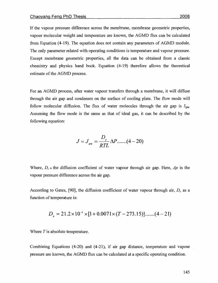
Chaovang Feng PhD Thesis 2008
If the vapour pressure difference across the membrane, membrane geometric properties,
vapour molecular weight and temperature are known, the AGMD flux can be calculated
from Equation (4-19). The equation does not contain any parameters of AGMD module.
The only parameter related with operating conditions is temperature and vapour pressure.
Except membrane geometric properties, all the data can be obtained from a classic
chemistry and physics hand book. Equation (4-19) therefore allows the theoretical
estimate of the AGMD process.
For an AGMD process, after water vapour transfers through a membrane, it will diffuse
through the air gap and condenses on the surface of cooling plate. The flow mode will
follow molecular diffusion. The flux of water molecules through the air gap is Jgap
Assuming the flow mode is the same as that of ideal gas, it can be described by the
following equation:
D J = J =^AP (4-20)
gap RTL
Where, Dp is the diffusion coefficient of water vapour through air gap. Here, Ap is the
vapour pressure difference across the air gap.
According to Gates, [90], the diffusion coefficient of water vapour through air, Dp, as a
function of temperature is:
Dp =21.2xl0-6x[l + 0.0071x(r-273.15)] (4-21)
Where T is absolute temperature.
Combining Equations (4-20) and (4-21), if air gap distance, temperature and vapour
pressure are known, the AGMD flux can be calculated at a specific operating condition.
145

Chaovang Feng PhD Thesis 2008
1.3. Heat transfer
As Fig. 4.2 shows, for an AGMD process, heat passes through the boundary layer on the
feed side to the surface of the membrane. On the surface, volatile component evaporates
and the vapour passes through membrane pore and air gap. At same time, heat will
transfer membrane and air gap. Finally, vapour condenses on the surface of the cooling
plate. Heat passes through the cooling plate and reaches the cooling stream. The
condensed liquid is removed so that the process can be carried on.
In order to simplify the analysis, the following assumptions are made:
a) Flow rate of cooling stream will not affect the warm feed concentration.
b) At the membrane surface of the warm feed side and at the surface of the cooling
plate, vapour and liquid are at equilibrium state.
c) Phase change resistance is much smaller than heat resistance.
d) Effect of concentration polarization is ignored.
A typical AGMD process is exactly following the diagram of Fig. 4.2. For an effective
membrane distillation system, where membrane thickness is S, membrane thermal
conductivity is km, air gap distance is L, thermal conductivity of air gap is &/, the
thickness of cool plate is 8P, thermal conductivity of cooling plate is fo, hot side
convection heat transfer coefficient is hf, and cool stream side convection heat transfer
coefficient is hPt heat transfer of AGMD can be described by the following analysis.
• Hot side boundary layer:
Q = hf(Tf-Tfm) (4-22)
Where, Q is heat flux from the warm feed to the membrane surface. T/ is the temperature
of the warm feed solution. Tm is the temperature on the membrane surface.
• Across membrane:
146

Chaoyanq Feng PhD Thesis 2008
Q = NxAH + ^(Tfm-TJ (4 -23) o
Where N is evaporated vapour flux, AH is latent heat of vaporization. 7}^ is the
temperature on the membrane surface. Tm is the temperature of membrane on other side;
km is the thermal conductivity of membrane.
• Across air gap :
Q = NxAH + ^(Tm-Tc) ( 4 - 24)
Where N is evaporated vapour flux. AH is latent heat of evaporation. Tm is the
temperature of membrane on the air gap side, ki is the thermal conductivity of air gap. Tc
is the temperature on the the surface, facing the air gap, of the cooling plate. As
mentioned before, heat transfer through condensed water film was ignored.
• Across cooling plate:
Q = ̂ (T-Tpc) ( 4 - 2 5 ) o
Where Tc is the temperature on the surface, facing the air gap, of cooling plate. Tpc is the
temperature of the surface, facing the cooling stream, of the cooling plate.
• Cooling stream boundary layer:
Q = h (T -T) (4-26)
147

Chaovanq Feng PhD Thesis 2008
Where Tpc is the temperature at the surface, facing cooling water of the cooling plate, Tp
is the bulk temperature of cooling stream.
Assuming evaporated vapour flux, N, is equal to membrane distillation permeate flux J, it
can be obtained from mass transfer analysis are from experiment. If the heat transfer
coefficients are known, and also the temperature of feed solution and the temperature of
the cooling stream are known, combining Equation (4-22) to Equation (4-26), the
temperatures at different surfaces of the AGMD process can be obtained. As an AGMD
module is chosen, the heat transfer coefficient related to the membrane material and the
AGMD configuration can be calculated. The latent heat for water can be found in the
literature.
The thermal conductivity of a porous membrane is represented by:
km={\-s)kmaterial+skg ( 4 - 2 7 )
Where, km is the thermal conductivity of the porous membrane, kmateriai is the thermal
conductivity of polymeric material, and kg is the thermal conductivity of air. As the
membrane thickness is known, the heat transfer coefficient of the porous membrane can
be given by:
h = ^=- ( 4 - 2 8 ) o
Where hm is the heat transfer coefficient of the porous membrane, and 5 is the thickness
of the membrane.
The hot side boundary layer heat transfer coefficient (/?/) and the cold side boundary layer
heat transfer coefficient (hp) are governed by the operating condition. Normally, the
boundary layer heat transfer coefficient is analogized with the mass transfer coefficient as
Nusselt number:
148

Chaovang Feng PhD Thesis 2008
Nu = aRebVrc (4-29)
• Re, Reynolds number Re =(/?• v» dh)lu (p: fluid density, v: fluid velocity, d/,:
hydraulic diameter, v : fluid viscosity)
• Pr, Prandtl number Pr= (Cp«//)/k (Cp: specific heat, u: fluid viscosity, k: thermal
conductivity )
For most of the fluid transfer, a, b, and c have the empirical values: i.e. a = 0.138 b=
0.672. c has two value. For hot fluid, c=0.3. For cool fluid, c=0.4. In AGMD process, the
boundary layer heat transfer coefficient can therefore be calculated as [91, 92]:
Nu = 0.138Re0672 Pr03 (4-30)
or
7Vrw = 0.138Re0672Pr04 (4-31)
Once the heat transfer coefficients are known, temperatures at the different surfaces of
the AGMD process can be obtained. As described before, the temperature difference
between two sides of membrane is the driving force for membrane distillation.
1.4. Temperature polarization
In a MD process, normally, a large energy flux increases the temperature difference
between the hot water bulk and the evaporating surface and between the evaporating
surface and the condensing surface, which leads to a smaller net driving temperature
difference between the evaporating and condensing water surfaces. This phenomenon is
known as temperature polarization, which reduces the water vapour flux.
149

Chaovanq Feng PhD Thesis 2008
Temperature polarization coefficient is generally used to quantify the magnitude of the
boundary layer resistances over the total heat transfer resistance. It is defined as:
0 = Zk_Zk (4-32) T -T lf 1 p
@, often used as indirect index of efficiency for MD process, falls between 0.4 and 0.7
for a satisfying design of the system [21], and approaches unity for mass transfer limited
operations.
In DCMD process, evaporation happens at hot side surface of membrane, while
condensation conducted at the surface of cooling side. Therefore, the temperature
polarization can be described by Equation (4-31). But in AGMD process, the evaporation
takes place at the hot side surface of membrane and the condensation takes place at the
surface of the cooling plate. The temperature polarization coefficient (© ') should include
membrane and air gap. Then,
O^Zk-ZL........... (4-33) Tf~TP
That means the membrane and the stagnant air film of air gap are the main resistances of
AGMD process. As shown in Figure 4.2, T m »T c , So, the value of 0 ' will larger than
the value of 0.
150
Chaovang Feng PhD Thesis 2008
2. THEORETICAL MODELING ANALYSIS OF AGMD FOR TWO VOLATILE
COMPONENTS (ETHANOL / WATER)
If the AGMD process involves two or more volatile components, the theoretical analysis
will become more complex. When two components are involved in AGMD process, such
as ethanol/water mixtures, the analysis of mass and heat transfer will still follow the
similar mechanism as that of a single component. Assuming each volatile component is
independent, i.e. the behaviour of evaporation and mass and heat transfer of each volatile
component are independent, the calculation follows that of the single volatile component.
2.1. Mass transfer
Since the theoretical analysis of mass transfer for a binary system is too complicated, it is
not attempted in this thesis. Rather, the experimental flux data for the components
(ethanol and water in this case) will be used in the following heat transfer analysis.
2.2. Heat transfer
All equations from Equation (4-22) to Equation (4-31) that have been derived for the one
volatile component system are applicable for the two component system, except;
a) To evaluate hfto be used in Equation (4-22), the physicochemical properties of the
ethanol/water mixture corresponding to the feed solution mixture should be used,
ignoring the concentration polarization.
b) AH in Equations (4-23) and (4-24) should correspond to that of the permeate
mixture. It is assumed that the latent heat of evaporation of a binary mixture is the
sum of the latent heat of evaporation weighed by the mole fraction of each
component.
151

Chaoyanq Feng PhD Thesis 2008
Then,
tefmiX=xw&Hw+xeAHe (4-34)
Where
And,
Therefore
water water
" water ' •*" water "" " ethanol ' -"* ethanol
x„ = •^ ertono/ ' -"" ethanol
J water ' •*" water ~*~ *̂ e(/iono/ ' "^ ethanol
\y water + ^ ethanol ) ^ ^ mix ~ ^ water ^ " w + J ethanol ^ 1 e
(4-35)
(4-36)
(4-37)
AHW, AHe and AHmjx are the latent heat of evaporation of water, ethanol and water-
ethanol mixture, respectively. Jwater and Jethanoi are the flux of water and ethanol,
respectively. xw and xe are mole fraction of water and ethanol in the permeate,
respectively.
2.3. Temperature polarization
Equation (4-33) can be used for the temperature polarization.
152

Chaoyang Feng PhD Thesis 2008
Chapter 5 AGMD SYSTEM AND EXPERINMENT
1. AGMD SYSTEM
The schematic representation of the AGMD system used is shown in Fig. 5-1:
Nanefiber Membrane Air gap
Feed Tank, Cooling Tank,
T, Condensation
Chamber
Permeate Tank
Figure 5.1 Diagram of AGMD system
The feed tank is immersed in a water bath to keep the feed solution temperature constant.
The cooling tank is also immersed in a water bath to keep the cooling side temperature
constant. The feed solution is recycled by the Masterflex Peristaltic Pump through the
feed chamber of the MD cell. The feed pressure is maintained lower than the liquid entry
pressure of water (LEPw), i.e. <5 psig. The air gap of the AGMD module is 2 mm.
Figure 5.2 shows the detailed structure of the AGMD module used in the current study.
153

Chaoyang Feng PhD Thesis 2008
Hot feed solution at a set temperature enters into the hot chamber from the centre tube,
passes through the separate wall in the middle of chamber, then enters into the tube at the
edge of the hot chamber and finally goes back to the feed tank. The cooling fluid at a set
temperature is pumped in to the cool chamber and then goes back to the cooling tank.
The cooling plate is made of aluminum.
Feed out*—c~:
Feed in
I i | I—'
I •m-, _ _
Cooling out
Cooling in
Permeate
Permeate
Figure 5.2 Diagram of AGMD module
2. MATERIALS AND METHODS
• PVDF nanofiber membrane
The PVDF nanofiber membrane was made by the electrospinning method. Details of the
membrane preparation and characterization are given in Part I. Some important
characterization parameters of the PVDF nanofiber membrane are:
1) Porosity: 76±5 %
154

Chaoyang Feng PhD Thesis 2008
2) Thickness: 0.15 mm
3) LEPw: 17.6 ±2 psig
4) Contact angle: >120°
5) Average pore size: 1.5 jam
• Feed solutions
Sodium chloride used in the current study was the food grade table salt from Sifto
Canada. Ethanol was supplied by Sigma-Aldrich (CR, 99%).
1) Sodium chloride solutions of 1, 3, 3.5, 6 and 22 wt% were used for desalination
by the AGMD system through PVDF nanofiber membrane.
2) Ethanol aqueous solutions of 5 and 10 wt% were used for ethanol concentration
by the AGMD system through PVDF nanofiber membrane.
3) Cooling fluid was water.
• Operating condition
Feed solution is pumped by Masterflex Peristaltic Pump. The feed solution flow rate is
600 mL/min. Feed pressure is 5 psig. The temperature of feed solution is set at a fixed
temperature (35, 43, 51, 60, 65, 71, 80°C). The cooling fluid flow flux is 6000 mL/min.
The cooling fluid temperature is set at 20 °C.
• Membrane distillation analysis
a) Desalination: Permeate of AGMD was measured by conductivity meter
(OAKTON® CON 11 Conductivity and TDS Meter, USA) to monitor the
concentration of NaCl. A series of NaCl solutions with different concentrations
(0-15% wt.) were prepared by distilled water.
As shown in Fig. 5.3, the conductivity of NaCl solution has a proportional
relationship with its concentration.
155

Chaoyanq Feng PhD Thesis 2008
In desalination experiments, sodium chloride concentrations (wt %) of the feed
and permeate solutions were measured by conductivity meter using a linear
calibration curve established between the solution conductivity and the sodium
chloride concentration. The salt rejection was calculated by:
„ . , NaCl concentra t ion in Permeate innn, , r 1N
Rejection = l x 100%. ...(5 - 1 ) NaCl concentrat ion in Feed
Conductivity calibration curve of NaCl solution
o to
o
o 3 -a a o o
200000
180000
160000
140000
120000
100000
80000
60000
40000
20000
0
y = 11346x
R2 = 0.9876
6 8 10 12 14
Concentration of NaCl (wt %)
Figure 5.3 Calibration curve of conductivity versus NaCl concentration
b) For the separation of ethanol/water mixtures the ethanol concentrations (5 and
10 wt %) in the feed and permeate were determined by measuring the weight of
the solution (50 mL) by an electronic balance at 25 °C. Then, the solution
density was calculated. The ethanol concentration was obtained by using the
data from CRC handbook [93] between the ethanol concentration (wt. %) and
the density of aqueous ethanol solution shown in Fig. 5.4.
The total permeation rate was obtained by weighing the permeate collected
156

Chaoyanq Feng PhD Thesis 2008
during a preset permeation period. The permeation flux was obtained by
dividing the permeation rate by the effective membrane area (115 cm").
1.2
o
! 0.6
•s 0 4
f 0.2 -
Concentration of Ethanol aqueous and Density at 25 °C (Data from CRC, Hand book of Chemistry and Physics)
y = -0.0021x+ 1.0084
R2 = 0.99
0 5 10 15 20 25 30 35 40 45 50 55 60 65 70 75 80 85 90 95 100
Concentration of Etahnol aqueous (wt%)
Figure 5.4 Calibration curve of density versus ethanol concentration
157

Chaovanq Feng PhD Thesis 2008
Chapter 6 RESULTS AND DISCUSSIONS
1. DESALINATION BY AGMD MEMBRANE DISTILLATION
1.1. Mass Transfer of AGMD
Theoretical analysis of the experimental data was conducted using Equations (4-18) and
(4-19). Equation (4-18) allows the theoretical calculation of the flux through the
membrane if appropriate membrane characterization parameters such as s, x and 5 are
known. Among those e and 8 are known experimentally and x is assumed to be equal to
unity. Furthermore, Yin, air is logarithmic mean mole fraction of air at the pore inlet and at
the pore outlet and can be obtained by knowing the respective water vapour pressures. As
for the pressure difference, Ap, it is unknown since the temperatures on both sides of the
membrane, Tfm and Tm, are unknown but in this analysis Tf and Tp were used instead,
knowing that it is only an approximation.
As expected, the theoretical results shown in Figs. 6.1 (flux versus vapour pressure
difference) and 6.2 (flux versus temperature difference) are in a linear and an exponential
form respectively and the magnitude of the flux is far greater than the experimental
values. Equation (4-20) also allows the flux calculation from the known air gap thickness
data. Again, this equation requires the vapour pressures corresponding to Tm and Tc, but
as an assumption those corresponding to Tf and Tp were used. The results are summarized
in Figs. 6.3 and 6.4 as linear and exponential forms. The experimental data obtained for
different feed NaCl concentrations are also shown in the figures. This shows that the
temperature (or pressure) differences used in the calculation are greater than the real
temperature (or pressure) differences.
Comparing Figs. 6.1 and 6.2 with Figs. 6.3 and 6.4, however, it can be said that equation
(4-20) resulted in an order of magnitude smaller flux values and they are closer to the
experimental ones. These results show that the difference between Tm and Tc is much
closer to Tf and Tp, which means most of the temperature, and vapour pressure, drop
158

Chaovang Feng PhD Thesis 2008
occurs in the air gap. Temperature drop in the membrane, on the other hand, is very
small.
110
188 95
70
TO
E
I Q s o <
55
40
15 1Q
y = 0.0023X + 2.0724 R2 = 0.9995
• AGMD flux calculated from Equation (4-19)
0 10000 20000 30000 40000 50000
AP, Water vapor pressure difference at feed and cooling temperature (Pa)
Figure 6.1 AGMD flux versus water vapour pressure difference (Flux calculated from
Equation (4-19))
140
•= 120
E -* 2 X 3 s=
rm
V Q. Q 5 O <
100
80
60
40
20
• AGMD flux calculated from Equation (4-19)
y = 4.6707e°051x
R2 = 0.9791
+ ^^~
jT •
• ^S"^ ^ •
5 10 15 20 25 30 35 40 45 50 55 60 65
AT, Temperature difference between feed solution and cooling fluid (°C) 70
Figure 6.2 AGMD flux versus temperature difference (Flux calculated from Equation (4-
19))
159

Chaovang Feng PhD Thesis 2008
2"
I •* X 3
•i. Q g o <
20
18
16
14
12
10
8
fi
4
2
0
• AGMD flux calculated from Equation (4-20)
• AGMD flux from 1 % NaCl solution
AGMD flux from 3.5 % NaCl solution
x AGMD flux from 6 % NaCl solution
X AGMD flux from 22 % NaCl solution
5000 10000 15000 20000 25000 30000 35000 40000 45000 50000
AP, Water vapor pressure difference at feed and cooling temperature (Pa)
Figure 6.3 AGMD flux versus water vapour pressure difference
<
18
16
14
12
10
8
6
4
2
0
•
•
&
X
X
-
AGMD flux calculated from Equation (4-20)
AGMD flux from 1% NaCl solution
AGMD flux from 3.5% NaCl solution
AGMD flux from 6% NaCl solution
AGMD flux from 22 % NaCl solution
•
+w*^Z-~~^£0
s s>
+/
/ m / h
/ s
> ^ V ) I !
/
10 15 20 25 30 35 40 45 50 55 60 65
AT, Temperature difference between feed solution and cooling fluid (°C)
70
Figure 6.4 AGMD flux versus temperature difference
Fluxes were either calculated from Equation (4-20) or obtained from experiments with 1,
3.5, 6, 22 wt % NaCl solutions.
160

Chaoyanq Feng PhD Thesis 2008
This conclusion is further confirmed by a more detailed analysis of the heat transport.
Based on the results, it also can be found that air gap governs the mass transport of
AGMD flux. With air gap increase, the AGMD flux will decrease quickly. Similar results
were reported by Kimura et al.[44].
1.2. Heat Transfer of AGMD
1.2.1. Heat transfer coefficient of hot side boundary layer
Temperature at each surface and temperature polarization can be calculated through
Equations (4-22)-(4-26). The heat transfer coefficient at each step of the heat transfer is
however required for this calculation.
The physico-chemical parameters used to obtain the heat transfer coefficients can be
found in the following references. 1) CRC Handbook of Chemistry and Physics [93], 2)
Lange's Handbook of Chemistry [94] (for example: THERMAL CONDUCTIVITY OF
AQUEOUS SOLUTIONS OF NaCl, VISCOSITY MEASUREMENTS OF ALCOHOL-
WATER MIXTURES AND THE STRUCTURE OF WATER).
The hot feed solution has a boundary layer, which affects the heat transfer from bulk
liquid to membrane surface (as shown in Fig. 4-2). The heat transfer coefficient of the
boundary layer can be obtained, similar to the mass transfer coefficient, using the
relationship between the dimensionless quantities such as shown by Equations (4-30) and
(4-31). It means heat transfer of AGMD is affected not only by the fluid property, but
also by the operating conditions.
The AGMD system used in this study is shown in Fig. 5.1. The flow rate of the feed
solution required in equations (4-30) and (4-31) was experimentally obtained. The basic
physicochemical properties for NaCl solution and ethanol/water mixture were obtained
from the literature.
161

Chaoyang Feng PhD Thesis 2008
1.2.2. Heat transfer coefficient of sodium chloride solution (hf)
The feed solution flow rate is 0.0197 m/s, the necessary physicochemical properties such
as density, viscosity, thermal conductivity etc. of NaCl solution are found in CRC
Handbook. Using these values in Equation (4-30) the heat transfer coefficient, hf, can be
calculated. Table 6.1 summarizes the heat transfer coefficient for NaCl solution, hf, for
different NaCl concentrations and temperatures.
Table 6.1 Heat transfer coefficient (hf) of NaCl solutions at different temperatures
NaCl solution
concentration
wt%
1
3
6
22
Heat transfer coefficient, hf_ (W/m2 K)
20 °C
189.3
189.2
189.0
175.8
30 °C
187.8
187.8
187.5
174.0
40 °C
186.6
186.7
186.2
173.0
60 °C
184.7
184.7
184.4
171.2
80 °C
184.2
183.5
183.2
167.0
100 °C
181.8
182.1
182.6
169.0
1.2.3. Heat transfer coefficient of ethanol aqueous solution (hf)
Similarly, the heat transfer coefficients for the ethanol/water mixtures can be calculated
from Equation (4-31). The results are summarized in Table 6.2.
Table 6.2 Heat transfer coefficient (hf) of aqueous ethanol solutions Ethanol
concentration wt%
1
2
3
4
5
6
7
8
9
10
Density kg/m3
996.3
994.5
992.7
991
989.3
987.8
986.2
984.7
983.3
981.9
Viscosity N.s/m2
0.000105
0.00011
0.000114
0.000118
0.000123
0.000128
0.000133
0.000139
0.000144
0.00015
Thermal conductivity W/mK
0.5900
0.5823
0.5747
0.5673
0.5599
0.5526
0.5454
0.5383
0.5313
0.5244
Heat transfer coefficient, hf
W/m2K
296.1
294.1
289.9
286.4
283.3
280.2
276.8
273.5
270.3
267.1
162

Chaovanq Feng PhD Thesis 2008
1.2.4. Heat transfer coefficient of PVDF nanofiber membrane (hm)
Thermal conductivity of PVDF polymer is 0.29 W/m K between 323 and 443 K (50 and
170°C) (data from the manufacturer [95]). Thermal conductivities of air are from CRC
Handbook of Chemistry and Physics, as shown in Table 6.3.
Table 6.3 Thermal conductivity of air
Name
Air
Thermal conductivity
(300 K),W/m K
0.0262
Thermal conductivity
(400 K), W/m K
0.0333
Thermal conductivities of water are also from CRC Handbook of Chemistry and Physics
[93], as shown in Table 6.4.
Table 6.4 Thermal conductivity of water
Temperature
°C
0
10
20
30
40
50
60
70
80
90
100
Vapour
pressure kPa
0.6
1.2
2.3
4.2
7.4
12.3
19.9
31.2
47.4
70.1
101.3
Thermal conductivity
(W/m K) (Liquid)
0.5610
0.5800
0.5984
0.6154
0.6305
0.6435
0.6543
0.6631
0.6700
0.6791
0.6821
Thermal conductivity
(W/m K) (Vapour)
0.01649
0.01721
0.01795
0.01870
0.01948
0.02028
0.02110
0.02196
0.02286
0.02380
0.02479
163

Chaovanq Feng PhD Thesis 2008
Both PVDF membrane thickness (0.15 mm) and porosity (0.76±4) were obtained
experimentally. Assuming that the PVDF nanofiber membrane pores are filled with air,
instead of water vapour, the heat transfer coefficient of PVDF nanofiber membrane was
calculated based on Equation (4-27). The results are shown in Table 6.5.
Table 6.5 Heat transfer coefficient (hm) of PVDF nanofiber membrane
Membrane
PVDF
hm
Heat transfer coefficient
(300 K),W/m2 K
596.7
Heat transfer coefficient
(400 K),W/m2 K
632.7
1.2.5. Heat transfer coefficient of air at air gap (hg = k^L)
The thermal conductivity of the air gap, ki, was obtained assuming the air gap was filled
with air. This can be justified since the highest average temperature of the air gap is 45°C
and the partial vapour pressure of water is 1/10 of atmospheric pressure. Since the
thickness of the air gap, L, is 2 mm, the heat transfer coefficient of the air gap, hg, can
also be calculated. The results are shown in Table 6.6.
Table 6.6 Heat transfer coefficient of air gap (hg)
Air gap
Air
Heat transfer coefficient (300 K),W/m2 K
8.73
\ Heat transfer coefficient
(400 K),W/m2 K 11.1
1.2.6. Heat transfer coefficient of cooling plate (hpiate = k2/5p)
The material of cooling plate is aluminum. The thickness is 5 mm. The thermal
conductivity of aluminum (237 W/m K) was obtained from CRC Handbook of Chemistry
and Physics. The heat transfer coefficient (hpiate) is therefore 47400 W/m2 K.
164

Chaoyang Feng PhD Thesis 2008
1.2.7. Heat transfer coefficient of cooling fluid boundary layer (hp)
The cooling fluid is water at room temperature (20 °C). The flow rate of cooling water is
0.644 m/s, obtained experimentally. Prandtl number of water was obtained from Perry's
Chemical Engineers' Handbook [96], as shown in Table 6.7. The physical properties of
water necessary for the calculation of heat transfer coefficients were obtained from CRC
Handbook of Chemistry and Physics, as shown in Table 6.8. Similar to the calculation of
hf, the dimensionless correlation (equation (4-31)) was used to calculate the Nusselt
number of the fluid, from which the heat transfer coefficient was calculated. The heat
transfer coefficient, hp, of boundary layer of cooling water at 20 °C was calculated to be
2725.2 W/m2 K.
Table 6.7 Prandtl number of water Pressure, bar
1 5 10 20
Perry's Chemical Eng
Prandtl number 300 K 5.81 5.82 5.82
ineers' Handbook (7th
350K 2.32 2.32 2.32
Edition) [96]
400K 0.98 1.34 1.34
Table 6.8 Physical properties of water at different temperatures
Temperature °C
0 10 20 30 40 50 60 70 80 90 100
Density g/cm
0.99984 0.99970 0.99821 0.99565 0.99222 0.98803 0.98320 0.97778 0.97182 0.96535 0.95840
Cp J/gK
4.2176 4.1921 4.1818 4.1784 4.1785 4.1806 4.1843 4.1895 4.1963 4.2050 4.2159
Vapour pressure
kPa 0.6113 1.2281 2.3388 4.2455 7.3814 12.344 19.932 31.176 47.373 70.117 101.325
Viscosity, \i Pas
1793 1307 1002 979.7 653.2 547.0 466.5 404.0 354.4 314.5 281.8
Thermal conductivity
W/Km 0.5610 0.5800 0.5984 0.6154 0.6305 0.6435 0.6543 0.6631 0.6700 0.6753 0.6791
165
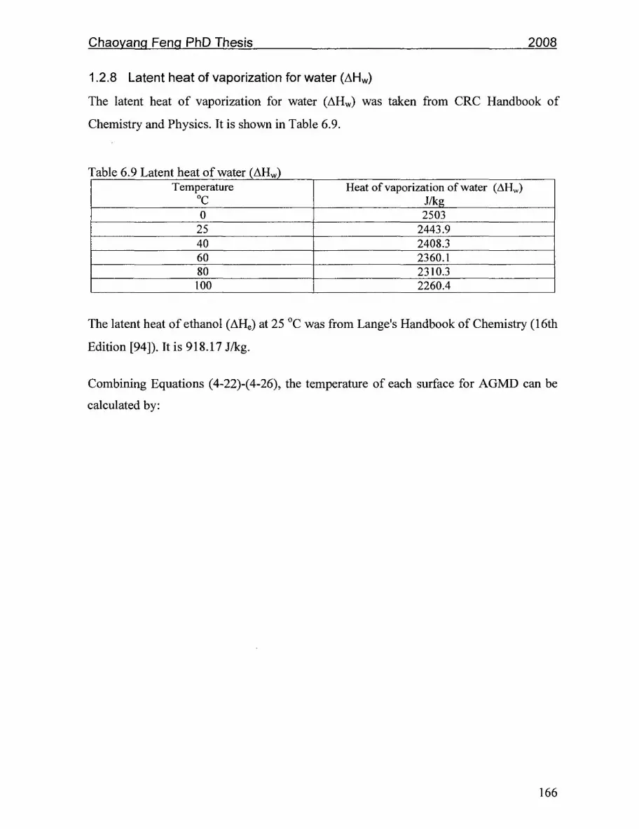
Chaovanq Feng PhD Thesis 2008
1.2.8 Latent heat of vaporization for water (AHW)
The latent heat of vaporization for water (AHW) was taken from CRC Handbook of
Chemistry and Physics. It is shown in Table 6.9.
' ̂ able 6.9 Latent heat of water (AHW) Temperature
°C 0
25 40 60 80 100
Heat of vaporization of water (AHW) J/kg 2503
2443.9 2408.3 2360.1 2310.3 2260.4
The latent heat of ethanol (AHe) at 25 °C was from Lange's Handbook of Chemistry (16th
Edition [94]). It is 918.17 J/kg.
Combining Equations (4-22)-(4-26), the temperature of each surface for AGMD can be
calculated by:
166

Chaovang Feng PhD Thesis 2008
T=Tn p p
T =T V V N=J
K K TcH—^xTvc—~xT» h p h p
"-plate "plate
Tm =(-^ +-^- +\)xTpc -!1^L -(-P- +^-)xT K Klate \ \ \late
T -• pc
K K K 1 1 K hn h„ (JL +JL + ^ +l)xr - ( - +-)xNxMw -(-2- +^ + ^ )
K K Klate K K Hn \ Klate
1 h u u u TfH^+y)xNxmw+(^^+^+^)xTp
( ^ + ^ + ^ + A + l ) L hn K K K K hplate K K K Klate
6-1 )
For a given set of experimental Tf and Tp values the vapour flux J was obtained either by
calculation (Equations (4-19) and (4-20)) or by experiments. Then, temperatures, Tc, Tm,
Tfm and Tpc were calculated by the above set of equations using the values for the heat
transfer coefficient and the latent heat of vaporization.
To simplify the calculation, a single value was used for the heat transfer coefficient at
each layer of the heat transfer resistance. As well, latent heat of vaporization at 25°C was
used. This approximation is to avoid the complicated iteration process. The used heat
transfer coefficient and heat of vaporization values are summarized in Table 6.10.
167

Chaovanq Feng PhD Thesis 2008
Table 6.10 Heat transfer coefficient and latent heat of vaporization for water used in
calculation hf
W/m2K 189.3
W/m2K 632.7
W/m2K 11.1
Opiate
W/m2K 47400
W/m2K 2725.1
J/kg 2443.9
AGMD fluxes calculated from Equations (4-19) and (4-20) are shown in Table 6.11
along with the experimental data. As mentioned earlier, agreement between the values
obtained from Equation (4-20) and the experimental values is much better than Equation
(4-19).
Table 6.11 Comparison of calculated and experimental AGMD fluxes
Temperature difference
AT (°C) 15 20 23 30 31 40 50 51 55 60
Vapour difference
AP (Pa) 3287.9 5042.6 5700.6 10005.2 8745.7 17593.2 22683.2 25497.1 28837.2 45034.2
AGMD Flux (kg/m2.h) Calculated
results from Equation (4-19)
8.6 13.0
25.1
42.8 54.4
68.1 103.4
Calculated results from
Equation (4-20) 1.10 1.71
3.47
6.23 8.11
10.40 16.53
Experiment results from NaCl solution
1% 1.53
2.06
3.13 4.80
6.45 8.23 11.63
3.50% 1.12
1.77
2.87 4.27
6.19 7.87 11.15
6% 1.33
2.05
2.47 3.82
4.87 6.19 10.17
22% 0.89
1.15
2.32 3.54
4.51 5.63 8.31
Both calculated values, from Equations (4-19) and (4-20), and the experimental flux
values were used to solve the set of equations given in (6.1) to obtain the temperatures at
different surfaces and the results summarized in Figures 6.5, 6.6 and 6.7 for the feed
temperature of 35, 50, and 80°C, respectively.
168

Chaovang Feng PhD Thesis 2008
o SB o DFlux from Equation (4-19)
DFlux from Equation (4-20) DFlux from 1% NaCl DFlux from 3.5% NaCl • Flux from 6% NaCl DFlux from 22% NaCl
Tfm Tm Tc Tpc Tp
Surface (position of AGMD Process
Figure 6.5 Temperature profile of AGMD process Feed temperature, 35°C; Cooling stream temperature, 20°C.
DFlux from Equation (4-19) DFlux from Equation (4-20) DFlux from 1% NaCl DFlux from 3.5% NaCl • Flux from 6% NaCl DFlux from 22% NaCl
Tf Tfm Tm T c T p c T p
Surface (position of AGMD Process
Figure 6.6 Temperature profile of AGMD process Feed temperature, 50°C; Cooling stream temperature, 20°C.
169

Chaovang Feng PhD Thesis 2008
•& CO
Tf Tfm Tm Tc Tpc Tp
Surface (pos i t i on of AGMD Process
DFlux from Equation (4-19) • Flux from Equation (4-20)
• Flux from 1% NaCl
• Flux from 3.5% NaCl
EFlux from 6% NaCl
• Flux from 22% NaCl
Figure 6.7 Temperature profile of AGMD process
Feed temperature, 80°C; Cooling stream temperature, 20°C.
All the above figures indicate that the major temperature drop occurs from Tm to Tc. This
is due to the smallest heat transfer value of air gap, hg (11.1 W/m K). There is also a
notable temperature drop from Tf to Tfm, reflecting the second smallest heat transfer value
of boundary layer on the feed solution side, hf (189.3 W/m2 K). The temperature drop
from Tfm to Tm across the membrane, which is the driving force for the vapour transport,
is so small, despite the fact that our current MD system has already achieved fluxes as
high as the commercial RO membranes (for example, FILMTEC RO membranes cover a
flux performance range from 1 to 14 1/m h bar) [97]. This heat transfer analysis
demonstrates clearly the possibility to achieve a significantly higher vapour flux than the
current values, if the AGMD system is properly designed to reduce the air gap resistance.
The temperature polarization coefficients, ®', were calculated according to Equation 4-33
and the results shown in Table 6.12. As the table shows the coefficients are above 0.94 in
all cases. However, these high values are rather misleading since only a small portion of
the temperature drop is utilized as the driving force for the vapour transport through the
membrane.
170

Chaovang Feng PhD Thesis 2008
Table 6.12 Temperature
AGMD
Flux from Equation (4-19)
Flux from Equation (4-20)
Flux from l%NaCl Flux from 3.5%
NaCl Flux from 22% NaCl
polarization coefficients (©') Temperature Polarization coefficient (©')
Feed temperature (35 °C)
0.9397
0.9415
0.9414
0.9415
0.9415
Feed temperature (50 °C)
0.9387
0.9413
0.9414
0.9414
0.9415
Feed temperature (80 °C)
0.9355
0.9408
0.9411
0.9411
0.9413
2. Salt Rejection of NaCl Solution by AGMD
As Fig. 6.8 shows, the salt rejection by the present AGMD system is over 97%.
Theoretically, the salt rejection should reach 100%. But the membrane for membrane
distillation in the current research has a pore size distribution, as shown in Part I, and
some pores are above the average pore size of 1.5 urn. Therefore the possibility of the
NaCl solution leakage through these large pores exists, which lowers the salt rejection
below 100%.
100
i 97
a s <
96
95
94
93
92
91
90
1 wt% NaCl solution
3.5 wt% NaCl solution
6 wt% NaCl solution
22 wt% NaCl solution
10 15 20 25 30 35 40 45 50
Temperature difference of AGMD(°C)
55 60 65
Figure 6.8 Salt rejection of NaCl solution by AGMD
171

Chaoyang Feng PhD Thesis 2008
3. Salt Rejection versus Concentration of NaCl Solution in Feed by AGMD
Figure 6.9 shows that NaCl rejection increases as the NaCl concentration in the feed
solution increases. This may be due to the increase in viscosity of the sodium chloride
solution, which lowers the flow rate of the solution through the large membrane pores.
Figure 6.9 Salt rejection versus concentration of NaCl solution
(Temperature difference of AGMD is 60 °C.)
4. Long Term Operation of AGMD
A 25-day separation test has been carried out and the data presented in Fig. 6.10. The
figure shows that NaCl rejection does not change considerably during the above
operational period. The latest data showed that the membrane was still applicable after
the above long term testing. It showed salt rejection of 99.9% for the feed NaCl
concentration of 22%.
172

Chaoyang Feng PhD Thesis 2008
102 101 100 99 98 97 96
b. 94 93
1_£_ ^-f 0-; --f* • • ^ » * Oi =•• • • • A *, <fc A * • ^ » V. J K A J
i i
'T» • • • • • • ; ' • • -
.. '
3.5% NaCI
6/0 NaUl
r 6% NaCI
1 % NaCI
£ 92
a 91 oT 90 "" 89 "5 88 W 87
86 85 84 83 82 81 80 0 1 2 3 4 5 6 7 8 9 10 11 12 1314 15 16 17 18 19 20 21 22 23 24 25 26 27 28 29 30
Operationl period (day)
Figure 6.10 Salt rejection versus operational period of AGMD
5. SEPARATION OF ETHANOL/WATER MIXTURES BY AGMD
5.1. Experimental results
AGMD was attempted by the PVDF nanofiber membrane for the alcohol/water mixtures
of 5 wt% and 10 wt% ethanol concentration. The mole fractions of ethanol in these
mixtures are 0.02 and 0.04, respectively.
The experimental flux data are given in Fig. 6.11. The permeate ethanol concentrations
are given in Fig. 6.12. It is clear that ethanol is concentrated in the permeate
considerably. As mentioned earlier, the ethanol concentration was determined by
measuring the solution density. The linear correlation between the ethanol concentration
and density was shown in Fig. 5.4. The data at different temperatures are summarized in
Table 6.13.
173

Chaovang Feng PhD Thesis 2008
^ 1 .
= > 1 . t — (
«-1. is «0. 0. 0. 0.
18
-AGMD flux from experimental result (5 wt. % ethanol aqueous) •AGMD flux from experimental result (10 wt.% aqueous)
20 22 24 26 28 30 32 34 36 38 40 42
Temperature differencr (°C)
Figure 6.11 AGMD flux for different temperature differences
Feed concentration of aqueous ethanol solutions, 5 wt% and 10 wt%.
24
to 22
g 20
a 18
° 16
g ft2 1 10 c
8 8 -3 6 c td 4. +->
« 2
0
3
— - — — • — " " —
n '
-•— ' —•
• —~~'~~
* Feed solution: 5 wt% ethanol aqueous
" Feed solution: 10 wt% ethanol aqueous
5 40 45 50 55
Feed solution temperature of AGMD (°C)
60 e 5
Figure 6.12 Ethanol concentration in the permeate at different temperature differences
Feed concentration of aqueous ethanol solutions, 5 wt% and 10 wt%.
Figure 6.13 is the Vapour Liquid Equilibrium (VLE) chart of ethanol-water binary
system from Handbook of Chemical and Environmental Engineering Calculations [98].
174

Chaovanq Feng PhD Thesis 2008
From the chart, as the mole fraction of ethanol in water is 0.02 (5 wt%) and 0.04 (10
wt%), in vapour phase the mole fraction of ethanol will be 0.1 and 0.18 respectively. It is
22.1 % and 35.9% in weight percentage from McCabe-Thiele diagram of ethanol water
system.
Figure 6.13 McCabe-Thiele diagram (VLE chart) of ethanol-water system [98]
Table 6.13 Density of aqueous ethanol solutions at different temperatures
Ethanol w t %
0 5 10 15 20 25 30 35 40 45 50 55 60 65 70 75 80 85 90 95 100
10 °C 0.9997 0.9910 0.9839 0.9780 0.9725 0.9666 0.9597 0.9516
0.9424 0.9322 0.9216 0.9105 0.8992 0.8877 0.8760 0.8641 0.8519 0.8395 0.8265 0.8128 0.7978
Density (g/cm 15 °C 0.9991 0.9903 0.9830 0.9767 0.9707 0.9642 0.9568
0.9483
0.9388 0.9285
0.9177 0.9066 0.8952 0.8836 0.8718 0.8599 0.8477 0.8352 0.8222 0.8085 0.7936
20 °C 0.9982 0.9894 0.9818 0.9751 0.9686 0.9617 0.9538
0.9449
0.9352 0.9247 0.9138 0.9026 0.8911 0.8795 0.8676 0.8556 0.8434 0.8393 0.8180 0.8042 0.7893
*) 25 °C 0.9971 0.9881 0.9804 0.9733 0.9664 0.9589 0.9506 0.9414
0.9315
0.9208 0.9098 0.8985 0.8870 0.8752 0.8634 0.8513 0.8391 0.8266 0.8136 0.7999 0.7850
30 °C 0.9957 0.9867 0.9787 0.9713 0.9639 0.9560 0.9474
0.9379
0.9277
0.9169 0.9058 0.8943 0.8828 0.8710 0.8591 0.8470 0.8347 0.8222 0.8092 0.7955 0.7807
175

Chaovang Feng PhD Thesis 2008
5.2. Heat transfer of AGMD
It is attempted again to obtain temperature profiles in the AGMD system by calculating
the temperatures at different surfaces. For this purpose, a set of equations (6-2) were
used. The difference between (6-1) and (6-2) is that water flux of (6-1) is replaced by the
combined ethanol and water flux in (6-2). As well, latent heat of vaporization of water is
replaced by the combined heat of vaporization of ethanol and water in (6-2), assuming
that the latent heat of the mixture is the sum of the product of the mole fraction and the
latent heat of vaporization of each component. The chosen heat transfer coefficient at
each heat barrier is given in Table 6.14 for 20°C. Comparing Tables 6.10 and 6.14, all
heat transfer coefficients are equal except for hf, which is natural because it was assumed
that the membrane pores and the air gap are filled with air in both desalination and
ethanol/water separation. This is a very crude assumption, which however allows us to go
around the tedious iteration procedure and yet provides us with a general picture of the
temperature profile in the system. The heating plate is aluminium and cooling media is
water in both experiments.
Table 6.14 Heat transfer coefficient and latent heat of vaporization for water and ethanol
used in the calculation hfof
aqueous ethanol
soln W/m2K
296.1
hm
W/m2K
632.7
W/m2K
11.1
hplate
W/m2K
47400
W/m2K
2725.2
AH of water J/kg
2443.9
AH of ethanol
J/kg
918.6
The results of AGMD flux for ethanol/water mixture from experiment are shown in Table
6.15.
Table 6.15 AGMD flux data obtained from AGMD experiments with aqueous ethanol
solutions Feed
Temperature (°C) 40 50 60
AGMD Flux (kg/mz.h) Experiment result from aqueous ethanol solutions
5 wt% 0.84 1.57 2.90
10wt% 0.94 1.75 3.14
176

Chaoyang Feng PhD Thesis 2008
T =T P P
T =T f f
N = J = J +J water ethanol
P P T =( + l)xT xT
c h pc h p plate plate
h h (j XAH +J xAH ) h h „ , P P ,. „ water w ethanol e P P % _ T =( + + l)xT - ( + )xT
m h h pc h h h p g plate g g plate
h h h h h h P P P 1 ! P P P
T =( +—•+ + l)xT - ( +—)x(J xAH +J xAH ) - ( + — + )xT fm h h h pc h h water w ethanol e h h h p
m g plate m g m g plate
1
pc h h h h . P P P P , , ( + + + + 1) h h h h
f m g plate
h h h h 1 1 p p p p
T +( + )x(J xAH +J xAH ) + ( + + + — — ) x T f h h water w ethanol e h h h h p
m g f m g plate
( 6-2 )
The temperature profiles are given in Figs. 6.14, 6.15 and 6.16. The temperature
polarization coefficients, 0 ' , are given in Table 6.16. These figures and the table are very
similar to Figures 6.5, 6.6 and 6.7 and Table 6.12, which were obtained for desalination.
The temperature polarization coefficients are also higher than 0.94.
Table 6.16 Temperature polarization coefficients (0 ')
AGMD
Flux from 5 wt% aqueous ethanol solution Flux from 10 wt% aqueous ethanol solution
Temperature Polarization coefl Feed temperature
(40 °C)
0.9439
0.9439
Feed temperature (50 °C)
0.9439
0.9438
ficient (©') Feed temperature
(60 °C)
0.9438
0.9438
177

Chaovanq Feng PhD Thesis 2008
Tem
pera
ture
of
ea
ch
surf
ace
in A
GMD
pro
cess
(°C
)
40
35
30
25
20
15 V / "7
=J
Tf " TfnT TnT
Surface (position) c
M
^ \
\ W — , — s
±±±± Tc Tpc
f AGMD Process
i
Tp A
• Flux from 5 wt% ethanol aqueous
DFlux from 10 wt% ethanol aqueous
Figure 6.14 Temperature profile of AGMD process with aqeous ethanol solution Feed temperature, 40°C; Cooling stream temperature, 20°C.
Te
mp
era
ture
o
f each
surf
ac
e in
AG
MD
pro
cess
(°
C)
50(—(
45
40
35
30
25
20
*-"''
y /
7 / 7 S—-f +.
15^ '-—^— 11
Sui
T
face
^ ~) / — Z /
/ -/ T fm Tm
(position) c
i- -/ /
>f AG
J. / /
/ / Tc Tpc
MD Process
• . r f
j
1
_jr Zi Tp
DFlux from 5 wt% ethanol aqueous
• Flux from 10 wt% ethanol aqueous
-/
Figure 6.15 Temperature profile of AGMD process with aqeous ethanol solution Feed temperature, 50°C; Cooling stream temperature, 20°C.

Chaovanq Feng PhD Thesis 2008
60 a s S 55 e
: so o
%? ^ : ~ 40 S M
^ | 35 O Q,
„ 30
I 25 s 20
/
* JS^~ 15 Tf
Sui
w \ \ \ \
V-\ \ " l i '| — i i
^TV-z-Z-^Tixxn T
rface
fm
(po
/ Tm
sition) <
Tc Tpc
>f AGMD Process
/ -1— nz
Tp
a Flux from 5 wt% ethanol aqueous
• Flux from 10 wt% ethanol aqueous
Figure 6.16 Temperature profile of AGMD process with aqueous ethanol solution Feed temperature, 60°C; Cooling stream temperature, 20°C.

Chaovanq Feng PhD Thesis 2008
Chapter 7 CONCLUSIONS OF AGMD MEMBRANE DISTILLATION
From the experimental results and the AGMD modeling analysis, the following
conclusions can be drawn.
1. Membrane distillation has a great potential as a novel separation process.
2. Membrane distillation can be used as an alternative method for desalination and
solution concentration.
3. PVDF nanofiber membrane fabricated by electrospinning can be used for membrane
distillation, particularly for AGMD.
4. The AGMD flux can be obtained with sufficiently high accuracy by equation (4-20)
that is based on the transport through the air gap.
5. Using 1 wt %, 3.5 wt%, 6 wt% and 22 wt% aqueous NaCl solutions as feed, the
highest AGMD flux achieved was 11 kg/m2 h. All the salt rejections were over 98.8
%. The long term running experiment showed that the PVDF nanofiber membrane
and the AGMD system were stable for at least 25 days. Thus, AGMD with the newly
developed PVDF nanofiber membrane seems to have a potential to compete with
commercial micro-filtration membranes.
6. The AGMD system with the newly developed PVDF nanofiber membrane also
enabled 5 wt % and 10 wt % aqueous ethanol solutions to be concentrated to 16 wt
% and 21 wt %, respectively, when the feed solution temperature was 60 °C. The
AGMD flux was about. 0.84-3.14 kg/m2»h
7. The temperature polarization coefficient defined by equation (4-33) is above 0.93 for
180

Chaovanq Feng PhD Thesis 2008
both single and two volatile components feed solutions. This is because the largest
heat resistance occurs at the air gap.
REFERENCES
1. D. Al-Gobaisi, (2000) Desalination and the Continuity of Human Civilization.
Watermark-The Newsletter of the Middle East Desalination Research Center, (9).
2. S.L. Postel, (2000) Water and world population growth. Journal of AWWA, 92 (4).
3. http://mvw.usbr.gov/pmts/water/publications/reportpdfs/reportQ72.pdf
4. S. A. Abdul-Wahab, J. Abdo, (2007) Optimization of multistage flash desalination
process by using a two-level factorial design Applied Thermal Engineering
27(2-3), Pages 413-421
5. O. K. Buros. (2000) The ABCs of Desalting. 2nd ed. Topsfield, MA: International
Desalination Association.
6. K. Wangnick, (2002) IDA Worldwide Desalting Plants Inventory. Report 2002,
Wangnick Consulting GMBH: Gnarrenburg, Germany.
7. C. Koroneos, A. Dompros, G. Roumbas, (2007) Renewable energy driven
desalination systems modelling Journal of Cleaner Production, 15(5), p 449-464
8. www.sandia.gov/water/docs/MillerSAND2003 0800.pdf
9. Roni F. Dalla Costa, Claudia W. Klein, Andrea M. Bernardes, Jane Zoppas Ferreira
(2002) Evaluation of the Electrodialysis Process for the Treatment of Metal
Finishing Wastewater, J. Braz. Chem. Soc. 13(4).
10. K. Lee, W. J. Koros, (2002) "Membranes, Synthetic, Applications." In Meyers, R.A.
(ed.). Encyclopedia of Physical Science and Technology. 3rd Edition. Academic
Press. New York, New York
11. E. Curcio, G. Di Profio, E. Drioli, (2002) Membrane crystallization of
macromolecular solutions Desalination, 145(1): p. 173-177.
12. K. Smolders, A. Franken, (1989) Terminology for Membrane Distillation
Desalination, 72: p. 249-262.
13. F. A. Banat, J. Simandl, (1999) Membrane distillation for dilute ethanol separation
from aqueous streams. Journal of Membrane Science, 163: p. 333-348.
14. M. C. Garcia-Payo, M. A. Izquierdo-Gil, C. Fernandez-Pineda, (2000) Air gap
181
Chaovang Feng PhD Thesis 2008
membrane distillation of aqueous alcohol solutions. Journal of Membrane Science,
169: p. 61-80.
15. M. C. Garcia-Payo, C. A. Rivier, I. W. Marison, U. V. Stockar, (2002) Separation of
binary mixtures by thermostatic sweeping gas membrane distillation. II.
Experimental results with aqueous formic acid solutions, J. Membr. Sci. 198, 197-
210.
16. M. Khayet, M. Godino, J. I. Mengual, (2003) Possibility of nuclear desalination
through various membrane distillation configurations: a comparative study.
International Journal of Nuclear Desalination, 1(1): p. 30-46.
17. A. M. Urtiaga, G. Ruiz and I. Ortiz, (2000) Kinetic analysis of the vacuum
membrane distillation of chloroform from aqueous solutions. Journal of Membrane
Science, 165: p. 99-110
18. E. Curcio, S. Simone, G. Di Profio, E. Drioli,.A. Cassetta, D. Lambac, (2005)
Membrane crystallization of lysozyme under forced solution flow. Journal of
Membrane Science 257, 134-143
19. N. Couffin, C. Cabassud, V. Lahoussine-Turcaud. (1998) A new process to remove
halogenated VOCs for drinking water production: vacuum membrane distillation.
Desalination, 117(1-3): 233-245.
20. K. W. Lawson, D. R. Lloyd, (1996) Membrane distillation .1. Module design and
performance evaluation using vacuum membrane distillation. Journal of Membrane
Science, 120(1): p. 111-121.
21. A. M. Alklaibi, Noam Lior, (2005) Membrane-distillation desalination: Status and
potential, Desalination, 171(2), p. 111-131
22. V. Soni, J. Abildskov, G. Jonsson, (2008) Modeling and analysis of vacuum
membrane distillation for the recovery of volatile aroma compounds from black
currant juice. Journal of membrane science, 320(1-2): p. 442-455.
23. S. Bandini, C. Gostoli, G. C. Sarti, (1992) Separation efficiency in vacuum
membrane distillation. Journal of Membrane Science, 73: p. 217-229.
24. D. Wirth, C. Cabassud, (2002) Water desalination using membrane distillation:
Comparison between inside/out and outside/in permeation, Desalination, 147: p. 139-
145.
182

Chaoyang Feng PhD Thesis 2008
25. K. W. Lawson, D. R. Lloyd, (1997) Membrane distillation: Review. Journal of
Membrane Science, 124: p. 1-25.
26. M. Galloway, J. Mahoney, (2004) Ultrafiltration for seawater reverse osmosis
pretreatment, Membrane Technology, p. 5-8.
27. K. Schneider, T. J. van Tassel, (1984) Membrane distillation. Chem.-Ing.-Tech, 56.
28. T. B. Mikhail, R. R. Nigmatullin, (1994) Membrane distillation, Russ. Chem. Rev.
63 1047-1062
29. W. Kunz, A. Benhabiles, R. Ben-Aim, (1996) Osmotic evaporation through
microprous hydrophobic membrane: a survey of current research and application.
Journal of membrane science, 121.
30. Z. Zhang, J. Gao, W. Zhang, Z. Ren, (2006) Experimental Study of the Effect of
Membrane Porosity on Membrane Absorption Process. Separation Science and
Technology, 41(14): p. 3245-3263.
31. United States Patent 5269836
32. United States Patent 4657743
33. X. Feng, R. Y. M. Huang, (1997) Liquid Separation by Membrane Pervaporation: A
Review. Ind. Eng. Chem. Res., 36(4): p. 1048-1066.
34. S. Zhang, (1995) Review: pervaporation membranes. Separation Science and
Technology, 30(1): p. 1-31.
35. M. Mulder, (1996) Basic Principles of Membrane Technology, 2 nd ed., Mulder, M.,
Dordrecht; Boston: Kluwer Academic Publishers.
36. D. W. Van Krevelen, (1990) Properties of Polymers,. 3rd Edition, Elsevier Science
Publishers, Amsterdam, Oxford, New York,
37. F. Banat, F. Abu Al-Rub, K. Bani-Melhem, (2003) Desalination by vacuum
membrane distillation: sensitivity analysis. Separation and Purification Technology,
33(1): p. 75-87.
38. S. Bandini, A. Saavedra, G. C. Sarti, V. Calabro, E. Drioli, (1997) Polarization
phenomena in integrated reverse osmosis and membrane distillation for seawater
desalination and waste water treatment. Desalination, 108(1-3): p. 81-82.
39. E. Drioli, Y. L. Wu, (1985) Membrane Distillation - an Experimental-Study.
Desalination, 53(1-3): p. 339-346.
183

Chaovanq Feng PhD Thesis 2008
40. C. M. Gujit, G. Raczi, J. W. Van Heuven, T. Reitht, A. B. De Haan, (1999)
Modelling of a transmembrane evaporation module for desalination of seawater.
Desalination, 126(1-3): p. 119-125.
41. W. T. Hanbury, T. Hodgkiess, (1985) Membrane Distillation - an Assessment.
Desalination, 56: p. 287-297.
42. S. T. Hsu, K. T. Cheng, J. S. Chiou, (2002) Seawater desalination by direct contact
membrane distillation. Desalination, 143(3): p. 279-287.
43. M. Khayet, M. Godino, J. I. Mengual, (2002) Thermal boundary layers in sweeping
gas membrane distillation processes. Alche Journal, 48(7): p. 1488-1497.
44. S. Kimura, S. I. Nakao, S. Shimatani, (1987) Transport Phenomena in Membrane
Distillation. Journal of Membrane Science, 33(3): p. 285-298.
45. F. Lagana, G. Barbieri, E. Drioli, (2000) Direct contact membrane distillation:
modelling and concentration experiments. Journal of Membrane Science, 166(1): p.
1-11.
46. K. W. Lawson, D. R. Lloyd, (1996) Membrane distillation .2. Direct contact MD.
Journal of Membrane Science, 120(1): p. 123-133.
47. G. L. Liu, C. Zhu, C. S. Cheung, C. W. Leung, (1998) Theoretical and experimental
studies on air gap membrane distillation. Heat and Mass Transfer, 34(4): p. 329-335.
48. L. Martinez, F.J. Florido-Diaz, (2001) Theoretical and experimental studies on
desalination using membrane distillation. Desalination, 139(1-3): p. 373-379.
49. G. C. Sarti, C. Gostoli, S. Matulli, (1985) Low energy cost desalination processes
using hydrophobic membranes. Desalination, 56: p. 277-286.
50. R. W. Schofield, A. G. Fane, C. J. D. Fell, (1987) Heat and Mass-Transfer in
Membrane Distillation. Journal of Membrane Science, 33(3): p. 299-313.
51. V. V. Ugrozov, I. B. Elkina, V. N. Nikulin, L. I. Kataeva, (2003) Theoretical and
experimental research of liquid-gap membrane distillation process in membrane
module. Desalination, 157(1-3): p. 325-331.
52. K. Schneider, W. Holz, R. Wollbeck, (1988) Membranes and modules for
transmembrane distillation. J. Membr. Sci, 39.
53. C. Gostoli, G. C. Sarti, S. Matulli (1987) Low temperature distillation through
hydrophobic membrane. Separation science and Technology, 22.
184

Chaovanq Feng PhD Thesis 2008
54. G. L. Morrison, A. G. Fane, P, Hogan. (1992) Solar heated membrane distillation, in
Proc. of the Biennial Congr. Of the Int. Solar Energy Soc. Sydney, Australia:
Pergamon.
55. P. A. Hogan, Sudjito, A. G. Fane, G. L. Morrison, (1991) Desalination by Solar
Heated Membrane Distillation. Desalination, 81(1-3): p. 81-90.
56. B. P. Konstantinos, N. L. Harris, (2001) Osmotic concentration of liquid foods
Journal of Food Engineering, 49(2-3), p. 201-206.
57. H. P. Hsieh, (2006) Membranes: Commercial Applications in Encyclopedia of
Surface and Colloid Science, edited by Ponisseril Somasundaran, CRC Press, ISBN
0849396042, 9780849396045.
58. P. Kober: (1917) Pervaporation, perstillation and percrystallization; J. Am. Chem.
Soc. 39: 944-950
59. United States Patent 3406096
60. United States Patent 3333583.
61. United States Patent 3340186.
62. M. E. Findley, V. V. Tanna, Y. B. Rao and C. L. Yeh, (1969) Mass and heat transfer
relations in evaporation through porous membranes, AIChE J., 15: 483-489.
63. A. Van Haute, Y. Henderyckx (1967) Permeability of membranes to water vapour
Desalination : 169-173
64. D. W. Gore, (1982) Gore-Tex membrane distillation, Proc. Tenth Ann. Convention
of the Water Supply Improvement Assoc, Honolulu, USA.
65. Enka/Membrane, (1984) Product literature.
66. A. S. Jonsson, R. Wimmerstedt, A.-C. Harrysson (Sweden) (1985) Membrane
distillation A theoretical study of evaporation through microporous
membranes, Desalination, 56:237-249.
67. W. T. Hanbury, T. Hodgkiess (UK) (1985) Membrane distillation An
assessment Desalination; 56: 287-297.
68. S. -I. Andersson, N. Kjellander, B. Rodesjs (Sweden) (1985) Design and field tests
of a new membrane distillation desalination process, Desalination, 56: 345-354.
69. L. Carlsson, (1983) The new generation in sea water desalination SU membrane
distillation system, Desalination, 45(2): 221-222.
185

Chaovang Feng PhD Thesis 2008
70. F. A. Banat, (1994) Membrane distillation for desalination and removal of volatile
organic compounds from water, in McGill University. McGill University: Montreal.
71. J. M. O. De Zaarate, A. Velazquez, L. Pena, J. I. Mengual, (1993) Influnence of
temperature polarization on sepoaration by membrane distillation. Separation science
and technology, 28.
72. R. C. Reid, J. M. Prausnitz, T. K. Sherwood, (1977) The Properties of Gases and
Liquids, 3rd edn. New York: McGraw-Hill.
73. S. Bandini, A. Saavedra, G. C. Sarti (1997) Separation Vacuum membrane
distillation: Experiments and modeling AIChE Journal, 43(2), p. 398 - 408
74. R. W. Schofield, A. G. Fane, C. J. D. Fell, (1987) Heat and mass transfer in
membrane distillation, J. Membrane Sci., 33, 299.
75. R. W. Schofield, A. G. Fane, C. J. D. Fell, (1990) Gas and vapour transport through
microporous membranes. II. Membrane distillation, J. Membrane Sci., 53, 173.
76. R. W. Schofield, A. G. Fane, C. J. D. Fell, (1990) Macounr, Factors affecting flux in
membrane distillation, Desalination, 77, 279.
77. M. Gryta. (2005) Osmotic MD and other membrane distillation variants Journal of
Membrane Science, 246(2), p. 145-156
78. P. J. Foster, A. Burgoyne, M. M. Vahdati, (2001) Improved process topology for
membrane distillation Separation and Purification Technology, 21(3), p. 205-217.
79. A. Katchalsky, P. P Curran, (1965) Non-equilibrium Thermodynamics in Biophysics,
Harvard University Press, Cambridge Massachusetts.
80. A. M. Alklaibia, N. Lior, (2006) Heat and mass transfer resistance analysis of
membrane distillation Journal of membrane science, 282, pp. 362-369
81. G. C. Sarti, C. Gostoli, (1989) Separation of liquid mixtures by membrane
distillation. Journal of Membrane Science, 33: p. 211-224.
82. G. C. Sarti, C. Gostoli, S. Bandini, (1993) Extraction of organic components from
aqueous streams by vacuum membrane distillation. Journal of Membrand Science,
80: p. 21-33.
83. A Saavedra, S. Bandini, G. C. Sarti, (1992) Separation of V.O.C. from aqueous
streams through vacuum membrane distillation. Euromembrane Conf., Paris, France.
84. R. W. Schofield, (1989) Membrane distillation, in The University of New South
186

Chaoyang Feng PhD Thesis 2008
Wales. The University of New South Wales.
85. C. Gostoli, G. C. Sarti, S. Matulli, (1987) Low temperature distillation through
hydrophobic membranes. Sep. Sci. Technol., 22: p. 855-872.
86. R. Datta, S. Dechapanichkul, J. S. Kim, L. Y. Fang, H. Uehara, (1992) A generalized
model for the transport of gases in porous, non-porous, and leaky membranes. I.
Application to single gases. Journal of Membrane Science, 75: p. 245-263.
87. E. A. Malinauskas, (1983) Gas Transport in Porous Media: The Dusty-Gas Model,
ed. S.W. Churchill. New York: Elsevier.
88. G. J. Geankoplis, (1993) Transport Processes and Unit Operations, 3rd ed.,Prentice
Hall, Englewood Cliffs, NJ.
89. M. Courel, M. Dornier, G. M. Rios, M. Reynes, (2000) Modelling of water transport
in osmotic distillation using asymmetric membrane Journal of Membrane Science,
173(1), p. 107-122
90. D. M. Gates, (1982) Biophysical ecology, Springer Verlag; New York, Heidelberg,
Berlin; 611 pp.
91. M. I. Vazquez-Gonzalez, L. Martinez (1994) Water distillation through
poly(tetrafluoroethylene) hydrophobic membranes in a stirred cell J. Chem. Soc,
Faraday Trans., 90, 2043 - 2046
92. G. W. Meindersma, C. M. Guijt, A. B. de Haan, (2006) Desalination and water
recycling by air gap membrane distillation. Desalination, 187, 291-301
93. CRC Handbook of Chemistry and Physics (1998) by David R. Lide (Editor) CRC-
Press; 79th edition.
94. Lange's Handbook of Chemistry (16th Edition). (2005) By: Speight, James G,
McGraw-Hill
95. http://www.arkema-inc.com/index.cfm?pag=622
96. Perry's Chemical Engineers* Handbook (7th Edition) (1997) Edited by: Perry, R.H.;
Green, D.W. McGraw-Hill.
97. fattp;//www.dow.eom/PublishedLiterature/dh 0042/0901b80380042dd8.pdf
98. Reynolds, Joseph P.; Jeris, John S.; Theodore, Louis Handbook of Chemical and
Environmental Engineering Calculations, 2002 John Wiley & Sons.
187

Chaoyang Feng PhD Thesis 2008
FUTURE RESEARCH WORKS
188

Chaovanq Feng PhD Thesis 2008
1. NANOFIBER MATERIAL RESEARCH
It has been shown in Part I that various naonofibers could be electrospun from different
polymers. Thus, the electrospinning technology is a simple, cheap and viable method to
fabricate nano-materials. Depending on the polymer, the nano-material has its own
specific application. The future research on electrospinning technology can be extended
to the following direction:
1) Material Development for Separation Processes
Novel nano-materials can be produced by electrospinning for separation applications
other than membrane distillation.
2) Material Development for Bio-engineering
Collagen nanofiber was successfully electrospun. It has a potential to be used for bio-
scaffold and drug release control. It may also be used for nerve guiding growth.
Possibility of electrospinning nanofibers from other biopolymers such as poly(lactide-co-
glycolide) (PLLG), Chitosan and poly(L-lactide) (PLLA) and so on, should also be
explored.
3) Development of Inorganic/Orgonic Blend Nanofibers
It would be interesting to blend Ti02, ZnO and other inorganic materials with polymers
to electrospin hybrid nano-materials. These composite materials have a great potential in
various applications due to considerably increased mechanical strength. For example,
electronspinning can spin continuous inorganic or particulate/polymer blend fibers with
nanoscaled diameters in the range of 50 to 5000 nm. Also those materials can be as a
precursor for making inorganic nanofiber.
4) Development of Carbon Nanofibers
PAN nanofibers have been successfully electrospun. It is known that the diameter of
PAN nanofiber can be reduced below 100 nm. PAN nanofibers can serve as a precursor
for carbon nanofibers.
189

Chaovang Feng PhD Thesis 2008
2. MEMBRANE DISTILLATION RESEARCH
It has been shown in Part II, PVDF nanofiber membrane was successfully applied for
membrane desalination by AGMD. Further research direction of AGMD by nanofiber
membranes is as follows:
1) Large scale AGMD Experiment
A pilot plant scale AGMD system needs to enable economic and engineering analysis of
AGMD by PVDF nanofiber membranes.
2) Module Design of AGMD
AGMD process performance is affected not only by the membrane, but also by the
module configulation and the system design. Optimization is necessary in both aspects to
maximize the performance of the AGMD process.
3) Research on Alcohol/Water Mixture and Other Applications
As shown in Part II, AGMD could be used for separation and concentration of
alcohol/water mixtures. Because of the complex nature of the binary system, modeling of
the heat and mass transfer was not done sufficiently in this thesis. This should be
accomplished in the future
4) Other Applications
As mentioned earlier, MD process also can be applied for food industrial, recycling and
reuse, heavy water treatment and industrial wastewater treatment. All thses possibilities
should be explored.
190

Chaoyang Feng PhD Thesis 2008
APPENDIX I
Microporous Polypropylene Membrane Development
for Desalination by Air Gap Membrane Distillation
191
Chaovanq Feng PhD Thesis 2008
1. INTRODUCTION
In membrane distillation process, a microporous hydrophobic membrane is in contact
with an aqueous heated solution on one side (feed or retentate). The hydrophobic nature
of the membrane prevents a mass transfer in liquid phase and creates a vapour-liquid
interface at the pore entrance. Here, volatile compounds evaporate, diffuse and/or convect
across the membrane pores, and are condensed and/or removed on the opposite side
(permeate or distillate) of the system. The nature of the driving force, in synergy with the
hydro-repellent character of the membrane, allows the complete rejection of non-volatile
solutes such as macromolecules, colloidal species, ions, etc. Lower temperatures and
pressures with respect to those usually used in conventional distillation column are
generally sufficient to establish a quite interesting trans-membrane flux, with consequent
reduction of energy costs and mechanical requirements of the membrane. Typical feed
temperatures vary in the range of 30-80 °C, thus permitting the efficient recycle of low-
grade or waste heat streams, as well as the use of alternative energy sources (solar, wind,
or geothermal). In addition, the possibility of using plastic equipment also reduces or
avoids erosion problems.
In MD, membrane is not involved in the transport phenomena on the basis of its selective
properties. Volatile compounds are transferred across the membrane according to vapour-
liquid equilibrium principia, whereas the microporous polymeric material acts as physical
barrier between two phases and sustains the interfaces where heat and matter are
simultaneously exchanged. Since the hydrophobic character of the membrane represents
a crucial requirement, membranes have to be made by polymers with a low value of
surface energy. Polymers such as polypropylene (PP), polytetrafluoroethylene (PTFE),
and polyvinylidenefluoride (PVDF) are commonly employed in the preparation of
membranes for MD applications. Microporous hydrophobic membranes are
manufactured by sintering, stretching, and phase inversion [1-3]: for instance, PP
membranes are generally prepared by stretching and thermal phase inversion, PTFE
membranes by sintering or stretching, PVDF membranes by phase inversion.
192
Chaovanq Feng PhD Thesis 2008
As polypropylene is cheaper and also has very high hydrophobic character. It was chosen
as initial polymer for fabricating novel MD membranes in the current research.
Microporous polypropylene membranes have a wide variety of applications as an
efficient material for separation. They are used in oxygenators [4], gas separation [5],
blood purification [6] and other aspects. So far two methods have been developed for the
preparation of microporous membranes. The traditional way is the stretch method [4].
Microvoids will form upon stretching of polymer because of the separation of the
lamellae. After heat-setting microporous membranes are obtained [7-12]. This process is
simple and easy to perform, but the distribution of membrane pore size is not easy to be
controlled. Another method to prepare microporous PP fiber membranes is through the
process of thermally induced phase separation (TIPS) [13]. A homogeneous solution is
formed at an elevated temperature by dissolving the polymer in a solvent with high-
boiling point and low molecular weight. The solution is cooled at a controlled rate or
quenched to induce phase separation. After the diluent is removed (typically by solvent
extraction) microporous hollow fiber membranes can be obtained [14-17]. However,
membranes formed via TIPS are somewhat fragile and a dense skin is easy to form
during TIPS process. Therefore, if the porosity is the same, the permeability of the
membranes formed via TIPS seems lower than those obtained via the stretch method.
The requirements for the MD membranes are high hydrophobic character and high
porosity. The objective of this work is to develop microporous PP membranes with high
hydrophobic character and high porosity by the wet phase inversion technique. More
specifically, PP is dissolved in a solvent together with a pore former. Xylene or kerosene
is chosen as the solvent since it is known that PP can be dissolved in the latter solvents at
a high temperature [18]. The PP solution is then cast into a film and the pore former is
leached out leaving a micro-porous structure. The porous PP membranes are further
characterised and tested for air gap membrane distillation.
193

Chaovanq Feng PhD Thesis : 2008
2. MATERIALS AND EXPERIMENTAL METHODS
2.1. Materials
The following materials were used for the experiments.
• Polymer Materials:
A: Syndiotactic: Polypropylene (PP), Mw=127K, (Sigma-Aldrich).
B: Isotactic: Polypropylene (PP), Mw=250K, (Sigma-Aldrich).
• Pore former (Additive):
PEG (polyethylene glycol) Mw=2,000, (Sigma-Aldrich).
PVP (polyvinyl pyrrolidone) Mw=l 0,000, (Sigma-Aldrich).
Docdecylbenzene Sulfonic Acid (DSA), (Sigma-Aldrich).
• Solvent:
Xylene (CP, Sigma-Aldrich).
Kerosene (CP, Sigma-Aldrich).
• Other chemicals:
NaCl (CP, Sigma-Aldrich).
2.2. Membrane preparation
1) Membrane Casting Solution Preparation
The method of membrane preparation is as follows.
7 g of polypropylene was added to 87-93 g of xylene or kerosene in a 250ml glass bottle
and the bottle was placed in an oven that was kept at 130 °C. When the polymer was
dissolved in the solvent, a clear solution was obtained. While keeping the solution at 130
°C, 3-6 g a pore former (either DSA, or PEG or PVP) was further added to the solution.
The solution was stirred at the high temperature to let the pore former and polymer be
mixed homogeneously. The compositions of the casting solutions are summarised in
Table 1.
194

Chaovanq Feng PhD Thesis 2008
Table 1 Composition of membrane casting solution
No.
1
2
3
4
5
6
7
8
9
10
11
12
Solvent
Xylene
Kerosene
Polymer
(PP)
Isotactic
Syndiatactic
Isotactic
Syndiatactic
Concentration
of Polymer
7 %
7 %
7 %
7 %
7 %
7 %
7 %
7 %
7 %
7 %
7 %
7 %
Concentration
of DSA
0
3%
0
0
3 %
0
0
3%
0
0
3%
0
Concentration
of PEG
0
0
3 %
0
0
3 %
0
0
3 %
0
0
3 %
Concentration
ofPVP
0
0
3 %
0
0
3 %
0
0
3 %
0
0
3%
2) Membrane casting
The polymer solution of high temperature prepared above was poured onto a glass plate
which was kept at 90°C. A casting bar designed and fabricated at the Chemical
Engineering shop was applied to spread the solution on the glass plate uniformly. After
the cast polymer solution film was cooled to the room temperature, it was dried in air for
48 hours. Then, the dry film together with the glass plate was immersed into water where
membrane was peeled off from the glass plate spontaneously. The membrane was further
washed in warm distilled water (60 °C) to leach out the pore former. The warm water was
changed every half hour for two hours. The membrane was air-dried prior to its
characterization and AGMD testing.
195

Chaovang Feng PhD Thesis 2008
2.3. Membrane Characterization
• Membrane thickness: Membrane thickness was measured by a micrometer
(COMBIMIKE, Mitutoyo MFG. CO., LTD. Japan). Measurement was made for
at least five different points of a membrane.
• Contact angle: The equilibrium contact angles were measured both for the dense
and the microporous membranes by Goniometer (ST, SCHERR TUMICO, USA).
Samples prepared for contact angle measurement were evenly placed on a glass
slide and fixed by plastic tape. The sample slide was mounted on the plate holder
for contact angle measurement. A water droplet (luL) came from a syringe needle
to the top surface of the membrane sample. Then, the equilibrium contact angle
was measured.
• Liquid entry pressure of water (LEPw): LEPw is the pressure that must be applied
to pure water before it penetrates into dried membrane pores. This pressure
depends on the pore size and the hydrophobicity of the membrane. LEPw is also a
limited pressure for operation by membrane distillation process.
• Membrane morphology: The membrane morphology was studied by Scanning
Electron Microscope (SEM) and Atomic Force Microscope (AFM): a) the
samples were pasted on a SEM sample holder with a double side carbon adhesive
tape. Then, they were put into a sputter-coating chamber to coat with PL, before
being subjected to SEM observation, b) AFM investigation was made by Digital
Instrument III, Multi-mode AFM.
2.4. Air Gap Membrane Distillation
In an AGMD process, only the feed solution is directly in contact with a membrane.
Permeate is condensed on a cooling surface. There is an air gap situated between the
membrane and the surface of the cooling chamber. The system used for AGMD is
schematically shown in Figure 1.
196

Chaoyang Feng PhD Thesis 2008
PP membrane / Air gap
Permeate Tank
Figure 1 Diagram of AGMD system
The feed which was recycled through the feed line, the cooling water (20 °C) was also
recycled. The permeate was collected in a permeate tank. The concentration of permeate
was monitored by a conductivity meter (CDM80, Radiometer A/S, Denmark). Based on
the NaCl concentration (when the feed is sodium chloride solution) of feed and permeate,
the salt rejection is obtained by:
Salt rejection = (1 concentrat ion in Permeate
concentrat ion in Feed ) x l 0 0 %
197

Chaovanq Feng PhD Thesis 2008
3. RESULTS AND DISCUSSION
3.1. Membrane Characterization
1) Thickness of membrane
The average thickness of membrane is shown in Table 2, where the membrane number is
the same as in Table 2.
Table 2 Thickness of PP membranes
No.
1
2
3
4
5
6
7
8
9
10
11
12
Solvent
Xylene
Kerosene
Polymer
Isotactic
Syndiatactic
Isotactic
Syndiatactic
Thickness of membrane (um)
153
147
138
116
128
115
137
112
109
126
118
106
From Table 2, the thicknesses of the membranes are in a range of 106-153 urn. No
particular trend is observed between the membrane thickness and the membrane
composition.
3.1.2. Contact angle of membrane
The equilibrium contact angle of the PP membranes is shown in Table 3.
198

Chaoyang Feng PhD Thesis 2008
Table 3 Contact angle of PP membranes
No.
1
2
3
4
5
6
7
8
9
10
11
12
Solvent
Xylene
Kerosene
Polymer
Isotactic
Syndiatactic
Isotactic
Syndiatactic
Contact angle (°)
110.3±3.3
87.6+2.7
83.5±1.6.
106.5+2.5
79.4+1.9
81.2+2.7
106.5+4.3
86.3+2.5
84.7+3.2
101.3+2.1
83.2+1.3
79.6+3.2
Table 3 shows that the contact angles of all the four dense films which were made from
the casing solutions without any pore formers are over 100°, regardless of the type of
polypropylene and the solvent used. Hence, polypropylene is intrinsically a very
hydrophobic polymer. But, the contact angles were considerably reduced when the
membranes were made from the casting solutions into which pore formers were added.
All of them showed contact angles lower than 90°. The high contact angle of the PP
films seems to be due to the dense structure of the film. On the other hand, the lower
contact angles of the porous PP membranes are due to the presence of micro-sized pores.
It is also possible that the pore formers could not be leached out completely because of
their hydrophobic nature, although they are not as hydrophobic as polypropylene
199

Chaovanq Feng PhD Thesis 2008
polymer, and the residual pore formers made the membrane surface a little bit more
hydrophilic.
3.1.3. Membrane Liquid entry pressure of water (LEPw)
Liquid entry pressure of water (LEPw) is a very important parameter of membranes when
they are applied for membrane distillation. The pressure of the feed chamber of the MD
setup should not be higher than LEPw, since otherwise the feed liquid will penetrate into
the membrane pores and wet the membrane. The method of LEPw measurement can be
found in Part I.
The LEPw of PP membranes is shown in Table 4.
Table 4 Liquid entry pressure of water (LEPw) of PP membranes
No.
1
2
3
4
5
6
7
8
9
10
11
12
Solvent
Xylene
Kerosene
Polymer
Isotactic
Syndiatactic
Isotactic
Syndiatactic
LEPw (psig )
93.3±3.1
39.7±2.3
46.3±3.2
108.2±2.5
38.6±5.2
42.3±1.6
87.3±4.6
36.211.5
47.4±3.6
96.3±2.8
38.6±1.7
43.613.3
200

Chaovanq Feng PhD Thesis 2008
Table 4 shows that, the LEPws of the membranes without pore former (membranes 1, 4,
7 and 10) are higher than 90 psig, except for membrane 7. On the other hand, the porous
membranes prepared from the casting solutions with pore formers have significantly
lower LEPw values (below 50 psig without exception).
3.1.4. Membrane Structure
a) SEM
Figure 2 shows the SEM images of all the studied PP membranes. Each PP membrane
made with a pore former clearly shows a porous structure. The membranes without pore
former (membranes 1, 4, 7, 10) have more dense structures. It is interesting to note that
no clear porous structures were observed for the latter membranes, even though LEPw
data were obtainable. Probably, those membranes also have porous structures, even
though they are not detected by SEM. Similar to the TIPS method, for which pores are
formed while a semi-crystal polymer solution is cooled by the phase separation, porous
structure could also be formed without any pore formers while the solvent is being
evaporated.
201

Chaoyang Feng PhD Thesis 2008
• * ' • • . • . • . > . . .
>v
SEM iniaee of membrane 1 SEM imase of membrane 2 SEM image of membrane 2
SEM iamse of membrane 4 SEM iniaee of membrane 5 SEM image of membrane 6
SEM image of membrane 7 SEM image of membrane 8 SEM image of membrane 9
• v "
••'''!". * . ' • , -
-;, *" .' , ,y. • ' . ' " •
:,-
\ '" 1 ' . " ' • . ' . '
• : • • • ' ; - : *
• : . - ' ! - . \
.^.._,_,,,, ' i . i . ' . : ' .• . . ' - . . ' i
• - ' i
; • : • •
" • • ' • ' • . T V P - ' " ? ; ' ; - " i i " , • ; -:-'>• ;
. : : . . * •
SEM image of membrane 10 SEM image of membrane 11 SEM image of membrane 12
Figure 2 SEM images of PP membranes
b) AFM
Figure 3 shows the AFM images of all the studied membranes. The pore structures of the
dense membranes (membranes 1, 4, 7 and 10) are clearly seen. Another interesting
202

Chaovanq Feng PhD Thesis 2008
observation is that the macromolecular nodules tend to aggregate when kerosene is used
as the solvent, while they tend to remain individual when xylene is used as the solvent.
v < /
• - # i V '
V
-•V i /
[ ett.QE) nsfdio - J=" X 0.550 at/iio
AFM image of membrane 1 AFM image of membrane 2 AFM image of membrane 3
a Bo.coa n*/ai.
^ > -v . .
>v".
,^>^.:«^7; • * * ! .
•»-y . - . • - • ^ > ' /
.̂̂ iV.. - ^ . « .
w x o.sas is^dt°
AFM image of membrane 4 AFM image of membrane 5 AFM image of membrane 6
J "^
V
•'W ^ = S U ^
g EQ.COQ iwdi«
AFM image of membrane 7 AFM image of membrane 8 AFM image of membrane 9
/ - V
-;^.y 1 / /
3 SO.CHI Rtfdtu '•f I E S
AFM image of membrane 10 AFM image of membrane 11 AFM image of membrane 12
Figure 3 AFM images of PP membrane
203

Chaovanq Feng PhD Thesis 2008
3.2. Membrane distillation
The results of AGMD experiments are given in Table 5. Either distilled water or 500ppm
NaCl solution was used as feed. Since the LEPw values of all the prepared membranes
were higher than 30 psig, the feed pressure was set equal to 30 psig. The temperature of
the feed water (solution) was 60 °C and the cooling water was 20 °C.
Table 5 AGMD membrane distillation
No.
1
2
3
4
5
6
7
8
9
10
11
12
Solvent
Xylene
Kerosene
Polymer
Isotactic
Syndiatactic
Isotactic
Syndiatactic
Pure Water
(L/m2.h)
0
27.6
28.3
0
26.5
30.7
0
28.4
31.2
0
36.6
29.4
NaCl 500ppm
Flux (L/m2.h)
0
18.9
19.4
0
17.2
23.2
0
15.5
26.4
0
23.2
21.3
Rejection %
-
23.6
37.6
-
33.8
43.7
-
39.6
46.3
-
31.2
43.1
The membranes prepared without adding pore formers (membrane 1,4,7 and 10) did not
show any evidence of membrane transport. It provides a strong evidence for the absence
of the obvious pores for the vapour transport. However, the membranes prepared with
pore formers showed some permeation. When the feed is distilled water, the flux of
permeate was higher than 26 kg/m2.h. When the feed is the NaCl solution, the permeate
flux was significantly lower than distilled water. The highest solute rejection value was
204

Chaovanq Feng PhD Thesis 2008
43.6 %. This dictates that some feed NaCl solution leaks through the pores of large sizes
in liquid form.
4. CONCLUSIONS
A number of works on fabricating microporous PP membrane for MD and other
application [19-22] have been made. This is still another attempt of fabricating PP
membranes of high hydrophobicity and high porosity based on the dry-wet phase
inversion technique. From the experimental results, the following conclusions have been
drawn:
1. Porous polypropylene membranes can be fabricated by the dry-wet phase
inversion technique when appropriate solvents, such as xylene and kerosene,
and pore formers, such as DSA, PEG and PVP, are used.
2. The membrane pore size is increased by adding a pore former.
3. Solvent has an effect on the membrane structure.
4. The AGMD fluxes of the membranes were 26.5-31.2 L/m2 h, when the feed was
distilled water, under the AGMD conditions used in this study. When the 500
ppm sodium chloride solution was used as feed, the fluxes were 15.5-26.4 L/m
h. The salt rejections were equal to or below 46.3%, indicating the leak of feed
solution through some of the membrane pores.
5. The microporous PP membranes fabricated by the present method are not
suitable for membrane distillation. But they may have applications in processes
other than membrane distillation.
REFERENCES
1. M. Mulder (1996) Basic Principles of Membrane Technology. Kluwer Academic
Publishers: Dordrecht.
2. D.R. Lloyd, K.E. Kinzer, H.S. Tseng, Microporous membrane formation via
thermally induced phase separation. I. Solid-liquid phase separation. J. Membr.
Sci., 52 (1990) 239-261.
205

Chaovanq Feng PhD Thesis 2008
3. M. Tomaszewska, Preparation and properties of flat-sheet membranes from
poly(vinylidene fluoride) for membrane distillation. Desalination (1996) 104:1-
11.
4. G.D. Reeder, B.G. Hattler, J. Rawleigh, F.R. Walters, Current progress in the
development of an intravenous membrane oxygenator, J. Am. Soc. Artif. Intern.
Organs 39 (1993) 461-465.
5. S. Berghmans, H. Berghmans, H.E.H. Meijer, Spinning of hollow porous fibers
via the TIPS mechanism, J. Membr. Sci. 116 (1996) 171-176.
6. P. Yuxin, S. Xinyuan, W. Qingrui, The present situation and development of
macromolecular membranes for purification of blood, Membr. Sci. Technol. 18
(1998)10-13.
7. M.L. Druin, J.T. Loft, S.G. Plovan, Novel open-celled microporous film, U.S.
Patent, 3,801,404, 1974.
8. R.J. Samuels, High strength elastic polypropylene, J. Polym. Sci., Polym. Phys.
Ed. 17(1979)535-568.
9. H.D. Noether, H. Brody, Low-modulus 'hard' elastic materials, Text. Res. J. 46
(1976) 467-478.
10. S.L. Cannon, W.O. Statton, The mechanical behavior of springy polypropylene,
Polym. Eng. Sci. 15 (1975) 633-645.
l l .H.S . Bierenbaum, R.B. Isaacson, M.L. Druin, S.G. Ploban, Microporous
polymeric films, Ind. Eng. Chem. Prod. Res. Develop. 13 (1974) 2-8.
12. J.J. Kim, T.S. Jang, Y.D. Kwon, U.Y. Kim, S.S. Kim, Structural study of
microporous polypropylene hollow fiber membranes made by the melt-spinning
and cold-stretching method, J. Membr. Sci. 93 (1994) 209-215.
13. A.J. Castro, Preparation of microporous polymer membranes via inverse phase
separation, U.S. Patent, 4247498,1981.
14. D.R. Lloyd, S.S. Kim, K.E. Krizer, Microporous membrane formation via
thermally induced phase separation, II. Liquid-liquid phase separation, J. Membr.
Sci. 64(1991)1-12.
206

Chaovanq Feng PhD Thesis 2008
15. S.S. Kim, D.R. Lloyd, Microporous membrane formation via thermally induced
phase separation, III. Effect of thermodynamic interaction on the structure of
isotactic polypropylene membranes, J. Membr. Sci. 64 (1993) 13-29.
16. G.B.A. Lim, S.S. Kim, Q. Ye, Y.F. Wang, D.R. Lloyd, Microporous membrane
formation via thermally induced phase separation, IV. Effect of isotactic
polypropylene crystallization on membrane structure, J. Membr. Sci. 64 (1991)
30^10.
17. S.S. Kim, G.B.A. Lim, A.A. Alwattari, Y.F. Wang, D.R. Lloyd, Microporous
membrane formation via thermally induced phase separation V. Effect of diluent
mobility and crystallization on the structure of isotactic polypropylene
membranes, J. Membr. Sci. 64 (1991) 41-68.
18. http://www.vp-scientific.com/pdfs/Resistance%20of%20Polvpropylene.pdf
19. S. Nago, Y. Mizutani, Microporous polypropylene hollow fiber with double
layers, J. Membr. Sci. 116 (1996) 1-7.
20. P. M. Atkinson, D. R. Lloyd, Anisotropic flat sheet membrane formation via
TIPS: atmospheric convection and polymer molecular weight effects, J. Membr.
Sci. 175(2000)225-238.
21. C. Chandavasu, M. Xanthos, K.K. Sirkar, C.G. Gogos, Fabrication of
microporous polymeric membranes by melt processing of immiscible blends, J.
Membr. Sci. 211 (2003) 167-175.
22. J.J. Kim, J.R. Hwang, U.Y. Kim, S.S. Kim, Operation parameters of melt
spinning of polypropylene hollow fiber membrane, J. Membr. Sci. 108 (1995)
25-36.
207

Chaoyang Feng PhD Thesis 2008
APPENDIX II
208

Chaoyang Feng PhD Thesis 2008
LIST OF ACRONYMS
AFM
AGMD
DCMD
DMAc
DMF
DNA
DSC
ED
EDR
GIBCO
GPa
HFP
IPA
IUPAC
KV
LEPw
MD
MED
MEE
MF
MSF
- Atomic Force Microscopy
- Air Gap Membrane Distillation
- Direct Contact Membrane Distillation
- Dimethyacetamide
- Dimethylformamide
- Deoxyribonucleic acid
- Differential Scanning Calorimetry
- Electro Dialysis
- Electrodialysis Reversal
- Nutrient Mixture (Ham)
-Gigapascal=106kPa
- Hexafluoro-2-propanol
- Isopropyl alcohol
- International Union of Pure and Applied Chemistry (1UPAQ)
- Kilo voltage
- Liquid Entry Pressure of Water
- Membrane distillation
- Multiple-effect distillation
- Multiple effect evaporation
- Microfiltration
- Multi stage flash
209

Chaovang Feng PhD Thesis 2008
MWCO - Molecular-weight cut off
Nomex (PA) - Polyamide (Dupont)
NSF - National Science Foundation
OD
PAN
PC
PE
PEI
PES
PLAGA
PLLG
PLLA
PP
PS
PTFE
PVA
PVC
PVDF
PVP
RO
SD1
SEM
SGMD
- Osmotic Distillation
- Polyacrylonitrile
- Polycarbonate
- polyethylene
- Polyetherimide
- Polyethersulphone
- poly(lactide-co-glycolide)
- poly(lactide-co-glycolide)
- Poly(-l-lactides)
- polypropylene
- polysulfone
- polytetrafluoroethylene
- Poly (vinyl alcohol)
- Poly (vinyl chloride)
- polyvinylidenefluoride
- Poly (vinylpyrrolidone)
- Reverse Osmosis
- Silt Density Index
- Scanning electronic micro
- Sweeping Gas Membrane
210

Chaoyang Feng PhD Thesis 2008
TDS - Total Dissolved Solid
Tg - Glass transition temperature
TIPS - Thermally Induced Phase Separation
Tm - Melt Temperature
TOC - Total Organic Carbon
UF - Ultrafiltration
VC - Vapour Compression
VMD - Vacuum Membrane Distillation
211

Chaovanq Feng PhD Thesis 2008
NOMENCLATURES
Greek Sympol:
fa]: Vc:
VT:
a:
5:
5p:
AH:
AHe:
AHw:
AP:
Ar e n t ry :
s:
So:
Yl:
Y2:
YL:
YLV:
YSL:
YSV:
TI:
Tlo:
X:
\i:
P :
\h-
Us:
Intrinsic Viscosity (dl/g)
Concentration Gradient (mol/l.m)
Temperature Gradient (K/m)
Constant of Transport
Membrane Thickness (m)
Thickness of Cool Plate (m)
Molar Latent Heat of Vapourization (J/kg)
Ethanol Latent Heat (J/kg)
Water Latent Heat (J/kg)
Across Membrane Vapour Pressure Difference (kPa)
Entry Pressure Difference (kPa)
Porosity
Vacuum Permittivity
Fraction
Fraction
Surface Tension of Solution (N/m)
Interfacial Tension of Liquid/Vapour (N/m)
Interfacial Tension of Solid/Liquid (N/m)
Interfacial Tension of Solid/Vapour (N/m)
Viscosity of Spinning Dope (cP)
Viscosity of Solvent (cP)
Molecule free path (m)
Fluid Viscosity (cP)
Fluid Viscosity (cP)
Mean Pore Diameter (m)
Mean Particle Size (m)
212

Chaovang Feng PhD Thesis 2008
9:
0:
0 ' :
e1:
e2: 9e:
p-
Pm:
Ppol:
CT:
ag:
dp.
<5s.
x:
Contact Angle
Temperature polarization coefficient
Temperature Polarization Coefficient
Contact Angle for Component 1
Contact Angle for Component 2
Effective Contact Angle
Fluid Density (g/1)
Density of Membrane (g/1)
Density of Polymer Material (g/1)
Surface Tension of Spraying Liquid (N/m)
Geometric Standard Deviation
Mean Diameter of Particle (m)
Mean Pore Diameter of Membrane (m)
Membrane Tortuosity
English sympol:
A:
Ao,
A1:
aj:
&water:
B:
B:
C:
C:
c:
Cr:
Cp:
Cp:
Constant
Intercept
Slope
Activity coefficient
Activity coefficient of water
Empirical coefficient
Constant
Constant
Liquid molar density
Polymer concentration (g/1)
Polystyrene latex suspension concentration in feed (g/1)
Polystyrene latex suspension concentration in permeate (g/1)
Specific heat capacity (J/kg.K)

Chaoyanq Feng PhD Thesis 2008
d: Droplet diameter (m)
D: Empirical coefficient
D : M a s s diffusion coefficient
d: Membrane pore d iameter (m)
dp: Pore size (m)
ds: Particle diameter (m)
E: Strength of electrical potential (V/m)
f: Solute rejection
hQ Heat transfer coefficient of air gap (W/nT.K)
hf: Hot side convect ion heat transfer coefficient ( W / m .K)
hm Heat transfer coefficient of P V D F nanofiber membrane ( W / m .K)
hp : Cool stream side convect ion heat transfer coefficient ( W / m .K)
J: Flux (kg/m2 .h)
k : Huggins—Martin constant
k: Heat conductivity (W/m.K)
k;: Heat conductivity o f air gap (W/m.K)
kite; Membrane heat conductivity of ethanol (W/m.K)
kjiW: Membrane heat conductivity of water (W/m.K)
ki; Thermal conductivity of cooling plate (W/m.K)
ICB: Boltzman constant
kg-. Thermal conductivi ty of air (W/m.K)
k,„ Membrane heat conductivi ty (W/m.K)
kmateriai: Heat conductivity of po lymer ic material (W/m.K)
Kn : Knudsen number
L: Heat diffusion coefficient
L: Air gap distance (m)
M : Water molar mass
N: Evaporated vapour flux
Ne: Evaporated ethanol vapours flux
Nw: Evaporated water vapour flux
Chaovanq Feng PhD Thesis 2008
P°: Liquid saturation pressure above a convex (kPa)
Pentry: Entry vapours pressure (kPa)
Piiq: Vapour partial pressure at liquid surface (kPa)
Pr: Prandtl number
Pvop: Vapour partial pressure close to the condensate surface (kPa)
Q: Charge of the particle
Q: Heat transfer from warm feed to membrane surface
R: Gas constant
Re: Reynolds number
rP, max: Largest pore size (m)
rp=: Membrane average pore size (m)
T: Temperature (K)
Ti Temperature of feed solution (K)
T2: Temperature of cooling side (K)
Tc: Temperature on the the surface, facing the air gap (K)
Tf: Temperature of warm feed solution (K)
Tjm: Temperature on the membrane surface (K)
Tg: Glass transition temperature (K)
Tm: Melt point temperature (K)
Tm: Temperature on the membrane surface (K)
Tm: Temperature of membrane (K)
Tp: Temperature of the surface, facing cooling stream, of the cooling plate (K)
Tp: Bulk temperature of cooling stream (K)
Tpc: Temperature at the surface, facing cooling water, of the cooling plate (K)
v: Fluid velocity (m /s)
VT: Total or bulk volume of material (m )
Vv: Volume of void-space (m3)
XNaCi: Mole fraction of sodium chloride
Yim Mole fraction of air at the pore inlet and at the pore outlet.
215