Embed Size (px)
Citation preview
DIABETIC RETINOPATHY CLASSIFICATION AND INTERPRETATION USING
DEEP LEARNING TECHNIQUES
Jordi De la Torre Gallart
ADVERTIMENT. L'accés als continguts d'aquesta tesi doctoral i la seva utilització ha de respectar els drets
de la persona autora. Pot ser utilitzada per a consulta o estudi personal, així com en activitats o materials d'investigació i docència en els termes establerts a l'art. 32 del Text Refós de la Llei de Propietat Intel·lectual (RDL 1/1996). Per altres utilitzacions es requereix l'autorització prèvia i expressa de la persona autora. En qualsevol cas, en la utilització dels seus continguts caldrà indicar de forma clara el nom i cognoms de la persona autora i el títol de la tesi doctoral. No s'autoritza la seva reproducció o altres formes d'explotació efectuades amb finalitats de lucre ni la seva comunicació pública des d'un lloc aliè al servei TDX. Tampoc s'autoritza la presentació del seu contingut en una finestra o marc aliè a TDX (framing). Aquesta reserva de drets afecta tant als continguts de la tesi com als seus resums i índexs. ADVERTENCIA. El acceso a los contenidos de esta tesis doctoral y su utilización debe respetar los
derechos de la persona autora. Puede ser utilizada para consulta o estudio personal, así como en actividades o materiales de investigación y docencia en los términos establecidos en el art. 32 del Texto Refundido de la Ley de Propiedad Intelectual (RDL 1/1996). Para otros usos se requiere la autorización previa y expresa de la persona autora. En cualquier caso, en la utilización de sus contenidos se deberá indicar de forma clara el nombre y apellidos de la persona autora y el título de la tesis doctoral. No se autoriza su reproducción u otras formas de explotación efectuadas con fines lucrativos ni su comunicación pública desde un sitio ajeno al servicio TDR. Tampoco se autoriza la presentación de su contenido en una ventana o marco ajeno a TDR (framing). Esta reserva de derechos afecta tanto al contenido de la tesis como a sus resúmenes e índices. WARNING. Access to the contents of this doctoral thesis and its use must respect the rights of the author. It
can be used for reference or private study, as well as research and learning activities or materials in the terms established by the 32nd article of the Spanish Consolidated Copyright Act (RDL 1/1996). Express and previous authorization of the author is required for any other uses. In any case, when using its content, full name of the author and title of the thesis must be clearly indicated. Reproduction or other forms of for profit use or public communication from outside TDX service is not allowed. Presentation of its content in a window or frame external to TDX (framing) is not authorized either. These rights affect both the content of the thesis and its abstracts and indexes.
Diabetic Retinopathy Classification and Interpretation using Deep Learning Techniques
JORDI DE LA TORRE GALLART
DOCTORAL THESIS2018
UNIVERSITAT ROVIRA I VIRGILI DIABETIC RETINOPATHY CLASSIFICATION AND INTERPRETATION USING DEEP LEARNING TECHNIQUES Jordi De la Torre Gallart

UNIVERSITAT ROVIRA I VIRGILI DIABETIC RETINOPATHY CLASSIFICATION AND INTERPRETATION USING DEEP LEARNING TECHNIQUES Jordi De la Torre Gallart
Diabetic Retinopathy Classificationand Interpretation using Deep
Learning Techniques
DOCTORAL THESIS
Author:Jordi DE LA TORRE GALLART
Supervisors:Dra. Aïda VALLS MATEU and
Dr. Domènec Savi PUIG VALLS
Department d’Enginyeria Informàtica i Matemàtiques
Tarragona2018
UNIVERSITAT ROVIRA I VIRGILI DIABETIC RETINOPATHY CLASSIFICATION AND INTERPRETATION USING DEEP LEARNING TECHNIQUES Jordi De la Torre Gallart

UNIVERSITAT ROVIRA I VIRGILI DIABETIC RETINOPATHY CLASSIFICATION AND INTERPRETATION USING DEEP LEARNING TECHNIQUES Jordi De la Torre Gallart
UNIVERSITAT ROVIRA I VIRGILI DIABETIC RETINOPATHY CLASSIFICATION AND INTERPRETATION USING DEEP LEARNING TECHNIQUES Jordi De la Torre Gallart

UNIVERSITAT ROVIRA I VIRGILI DIABETIC RETINOPATHY CLASSIFICATION AND INTERPRETATION USING DEEP LEARNING TECHNIQUES Jordi De la Torre Gallart

v
To my wife Ana,my children Pol & Alba,
my parents José & Tere andmy siblings Sonia, Xavi & Sergi.
UNIVERSITAT ROVIRA I VIRGILI DIABETIC RETINOPATHY CLASSIFICATION AND INTERPRETATION USING DEEP LEARNING TECHNIQUES Jordi De la Torre Gallart

UNIVERSITAT ROVIRA I VIRGILI DIABETIC RETINOPATHY CLASSIFICATION AND INTERPRETATION USING DEEP LEARNING TECHNIQUES Jordi De la Torre Gallart
vii
“Study hard what interests you the most in the most undisciplined, irreverent andoriginal manner possible.”
Richard Feynman
“El amor al saber, la curiosidad, el asombro, es lo que puede sostener a cualquierser humano.”
Antonio Escohotado
“The process of creativity and genius are inherent in human consciousness.”
David R. Hawkins
“Nada para mí que no sea para los otros.”
Alejandro Jodorowsky
UNIVERSITAT ROVIRA I VIRGILI DIABETIC RETINOPATHY CLASSIFICATION AND INTERPRETATION USING DEEP LEARNING TECHNIQUES Jordi De la Torre Gallart

UNIVERSITAT ROVIRA I VIRGILI DIABETIC RETINOPATHY CLASSIFICATION AND INTERPRETATION USING DEEP LEARNING TECHNIQUES Jordi De la Torre Gallart
ix
AcknowledgementsThis work is supported by the URV grant 2015PFR-URV-B2-60 and the
Spanish research projects PI15/01150 and PI12/01535 (Instituto Salud Car-los III).
I would like to express my gratitude to my supervisors Dra. Aïda Vallsand Dr. Domènec Puig for their useful guidance, insightful comments, andconsiderable encouragement to complete this thesis.
I would also like to express my gratitude to Dr. Pere Romero-Aroca andhis team of collaborators of the Hospital Universitari Sant Joan de Reus,for their trust, passion and for providing the medical interpretation assess-ment required in this thesis.
I would also like to thank to all the Artificial Intelligence Community,specially to Geoffrey Hinton, Yann LeCun, Yoshua Bengio and Andrew Ng,an example to follow for their proved generosity sharing their knowledgein benefit of all Humanity.
My gratitude also for Facebook Inc. and Google Inc., technologicalleader companies in favor of public research, collaborating, designing andpublicly sharing freely important part of their research and their machinelearning tools: PyTorch and Tensorflow, helping to speed up immenselythe creation of greatly beneficial products for all of us.
My gratitude for all the Open Source Community. Culture of collabo-ration is key for our success as Civilization.
Without all of them this thesis would not be possible.
UNIVERSITAT ROVIRA I VIRGILI DIABETIC RETINOPATHY CLASSIFICATION AND INTERPRETATION USING DEEP LEARNING TECHNIQUES Jordi De la Torre Gallart

UNIVERSITAT ROVIRA I VIRGILI DIABETIC RETINOPATHY CLASSIFICATION AND INTERPRETATION USING DEEP LEARNING TECHNIQUES Jordi De la Torre Gallart
xi
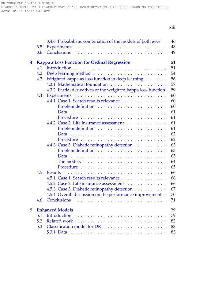
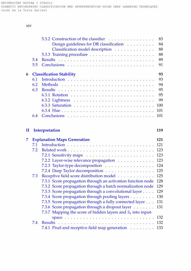
Contents
Acknowledgements ix
List of Figures xvii
List of Tables xxi
Abstract xxv
1 Introduction 11.1 Motivation . . . . . . . . . . . . . . . . . . . . . . . . . . . . . 11.2 Objectives . . . . . . . . . . . . . . . . . . . . . . . . . . . . . 3
1.2.1 Design of a DR classifier . . . . . . . . . . . . . . . . . . 31.2.2 Design of a system for results interpretation . . . . . . 41.2.3 Design a model for facilitating the understanding of
explanations . . . . . . . . . . . . . . . . . . . . . . . . . 41.3 Contributions . . . . . . . . . . . . . . . . . . . . . . . . . . . 51.4 Thesis organization . . . . . . . . . . . . . . . . . . . . . . . . 6
2 Background 72.1 Diabetic retinopathy . . . . . . . . . . . . . . . . . . . . . . . 7
2.1.1 Retina health evaluation . . . . . . . . . . . . . . . . . . 9Fundus photography . . . . . . . . . . . . . . . . . . . . 10
2.1.2 Diabetic retinopathy grading and classification . . . . . 112.2 Evaluation measures for disease grading . . . . . . . . . . . . 14
2.2.1 Confusion matrix . . . . . . . . . . . . . . . . . . . . . . 152.2.2 Sensitivity and Specificity . . . . . . . . . . . . . . . . . 162.2.3 Positive and Negative Predictive Value . . . . . . . . . 162.2.4 False Positive and Negative Rates . . . . . . . . . . . . 172.2.5 False Discovery and Omission Rates . . . . . . . . . . . 17
UNIVERSITAT ROVIRA I VIRGILI DIABETIC RETINOPATHY CLASSIFICATION AND INTERPRETATION USING DEEP LEARNING TECHNIQUES Jordi De la Torre Gallart
xii
2.2.6 Accuracy . . . . . . . . . . . . . . . . . . . . . . . . . . . 182.2.7 Balanced measures . . . . . . . . . . . . . . . . . . . . . 182.2.8 The Kappa family of statistics . . . . . . . . . . . . . . . 192.2.9 How to define human performance . . . . . . . . . . . 21
2.3 Machine Learning . . . . . . . . . . . . . . . . . . . . . . . . . 212.3.1 Supervised Learning . . . . . . . . . . . . . . . . . . . . 22
Classification vs Regression . . . . . . . . . . . . . . . . 22Dataset management . . . . . . . . . . . . . . . . . . . . 23Strategies for hyper-parameter optimization . . . . . . 23
2.3.2 Algorithms used in supervised machine learning . . . 242.3.3 Pattern recognition . . . . . . . . . . . . . . . . . . . . . 26
Traditional models of pattern recognition . . . . . . . . 26Deep Learning for pattern recognition . . . . . . . . . . 26Types of Deep Learning architectures . . . . . . . . . . 27Convolutional neural networks . . . . . . . . . . . . . . 27
2.3.4 Prediction error: bias vs variance . . . . . . . . . . . . . 312.3.5 Model ensembling . . . . . . . . . . . . . . . . . . . . . 32
2.4 Data . . . . . . . . . . . . . . . . . . . . . . . . . . . . . . . . . 332.4.1 Datasets . . . . . . . . . . . . . . . . . . . . . . . . . . . 332.4.2 EyePACS dataset . . . . . . . . . . . . . . . . . . . . . . 342.4.3 Messidor-2 dataset . . . . . . . . . . . . . . . . . . . . . 342.4.4 HUSJR dataset . . . . . . . . . . . . . . . . . . . . . . . 34
2.5 Summary of the data and methods used in this thesis . . . . 35
I Classification 37
3 Preliminary Models 393.1 Introduction . . . . . . . . . . . . . . . . . . . . . . . . . . . . 393.2 Related work . . . . . . . . . . . . . . . . . . . . . . . . . . . . 403.3 Data . . . . . . . . . . . . . . . . . . . . . . . . . . . . . . . . . 413.4 Methodology for retinal image classification . . . . . . . . . . 41
3.4.1 Evaluation function . . . . . . . . . . . . . . . . . . . . 423.4.2 Data pre-processing and data augmentation . . . . . . 433.4.3 Model . . . . . . . . . . . . . . . . . . . . . . . . . . . . 433.4.4 Training procedure . . . . . . . . . . . . . . . . . . . . . 443.4.5 Testing procedure . . . . . . . . . . . . . . . . . . . . . . 45
UNIVERSITAT ROVIRA I VIRGILI DIABETIC RETINOPATHY CLASSIFICATION AND INTERPRETATION USING DEEP LEARNING TECHNIQUES Jordi De la Torre Gallart
xiii
3.4.6 Probabilistic combination of the models of both eyes . 463.5 Experiments . . . . . . . . . . . . . . . . . . . . . . . . . . . . 483.6 Conclusions . . . . . . . . . . . . . . . . . . . . . . . . . . . . 49
4 Kappa a Loss Function for Ordinal Regression 514.1 Introduction . . . . . . . . . . . . . . . . . . . . . . . . . . . . 514.2 Deep learning method . . . . . . . . . . . . . . . . . . . . . . 544.3 Weighted kappa as loss function in deep learning . . . . . . 56
4.3.1 Mathematical foundation . . . . . . . . . . . . . . . . . 574.3.2 Partial derivatives of the weighted kappa loss function 59
4.4 Experiments . . . . . . . . . . . . . . . . . . . . . . . . . . . . 604.4.1 Case 1. Search results relevance . . . . . . . . . . . . . . 60
Problem definition . . . . . . . . . . . . . . . . . . . . . 60Data . . . . . . . . . . . . . . . . . . . . . . . . . . . . . 61Procedure . . . . . . . . . . . . . . . . . . . . . . . . . . 61
4.4.2 Case 2. Life insurance assessment . . . . . . . . . . . . 61Problem definition . . . . . . . . . . . . . . . . . . . . . 61Data . . . . . . . . . . . . . . . . . . . . . . . . . . . . . 62Procedure . . . . . . . . . . . . . . . . . . . . . . . . . . 62
4.4.3 Case 3. Diabetic retinopathy detection . . . . . . . . . . 63Problem definition . . . . . . . . . . . . . . . . . . . . . 63Data . . . . . . . . . . . . . . . . . . . . . . . . . . . . . 63The models . . . . . . . . . . . . . . . . . . . . . . . . . 64Procedure . . . . . . . . . . . . . . . . . . . . . . . . . . 65
4.5 Results . . . . . . . . . . . . . . . . . . . . . . . . . . . . . . . 664.5.1 Case 1. Search results relevance . . . . . . . . . . . . . . 664.5.2 Case 2. Life insurance assessment . . . . . . . . . . . . 664.5.3 Case 3. Diabetic retinopathy detection . . . . . . . . . . 674.5.4 Overall discussion on the performance improvement . 70
4.6 Conclusions . . . . . . . . . . . . . . . . . . . . . . . . . . . . 71
5 Enhanced Models 795.1 Introduction . . . . . . . . . . . . . . . . . . . . . . . . . . . . 795.2 Related work . . . . . . . . . . . . . . . . . . . . . . . . . . . . 825.3 Classification model for DR . . . . . . . . . . . . . . . . . . . 83
5.3.1 Data . . . . . . . . . . . . . . . . . . . . . . . . . . . . . 83
UNIVERSITAT ROVIRA I VIRGILI DIABETIC RETINOPATHY CLASSIFICATION AND INTERPRETATION USING DEEP LEARNING TECHNIQUES Jordi De la Torre Gallart
xiv
5.3.2 Construction of the classifier . . . . . . . . . . . . . . . 83Design guidelines for DR classification . . . . . . . . . 84Classification model description . . . . . . . . . . . . . 88
5.3.3 Training procedure . . . . . . . . . . . . . . . . . . . . . 885.4 Results . . . . . . . . . . . . . . . . . . . . . . . . . . . . . . . 895.5 Conclusions . . . . . . . . . . . . . . . . . . . . . . . . . . . . 91
6 Classification Stability 936.1 Introduction . . . . . . . . . . . . . . . . . . . . . . . . . . . . 936.2 Methods . . . . . . . . . . . . . . . . . . . . . . . . . . . . . . 946.3 Results . . . . . . . . . . . . . . . . . . . . . . . . . . . . . . . 95
6.3.1 Rotation . . . . . . . . . . . . . . . . . . . . . . . . . . . 956.3.2 Lightness . . . . . . . . . . . . . . . . . . . . . . . . . . 996.3.3 Saturation . . . . . . . . . . . . . . . . . . . . . . . . . . 1006.3.4 Hue . . . . . . . . . . . . . . . . . . . . . . . . . . . . . . 101
6.4 Conclusions . . . . . . . . . . . . . . . . . . . . . . . . . . . . 101
II Interpretation 119
7 Explanation Maps Generation 1217.1 Introduction . . . . . . . . . . . . . . . . . . . . . . . . . . . . 1217.2 Related work . . . . . . . . . . . . . . . . . . . . . . . . . . . . 123
7.2.1 Sensitivity maps . . . . . . . . . . . . . . . . . . . . . . 1237.2.2 Layer-wise relevance propagation . . . . . . . . . . . . 1237.2.3 Taylor-type decomposition . . . . . . . . . . . . . . . . 1247.2.4 Deep Taylor decomposition . . . . . . . . . . . . . . . . 125
7.3 Receptive field score distribution model . . . . . . . . . . . . 1257.3.1 Score propagation through an activation function node 1287.3.2 Score propagation through a batch normalization node 1297.3.3 Score propagation through a convolutional layer . . . . 1297.3.4 Score propagation through pooling layers . . . . . . . . 1307.3.5 Score propagation through a fully connected layer . . . 1317.3.6 Score propagation through a dropout layer . . . . . . . 1317.3.7 Mapping the score of hidden layers and Sk into input-
space . . . . . . . . . . . . . . . . . . . . . . . . . . . . . 1327.4 Results . . . . . . . . . . . . . . . . . . . . . . . . . . . . . . . 132
7.4.1 Pixel and receptive field map generation . . . . . . . . 133
UNIVERSITAT ROVIRA I VIRGILI DIABETIC RETINOPATHY CLASSIFICATION AND INTERPRETATION USING DEEP LEARNING TECHNIQUES Jordi De la Torre Gallart
xv
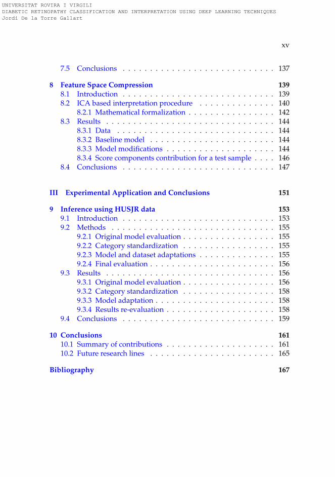
7.5 Conclusions . . . . . . . . . . . . . . . . . . . . . . . . . . . . 137
8 Feature Space Compression 1398.1 Introduction . . . . . . . . . . . . . . . . . . . . . . . . . . . . 1398.2 ICA based interpretation procedure . . . . . . . . . . . . . . 140
8.2.1 Mathematical formalization . . . . . . . . . . . . . . . . 1428.3 Results . . . . . . . . . . . . . . . . . . . . . . . . . . . . . . . 144
8.3.1 Data . . . . . . . . . . . . . . . . . . . . . . . . . . . . . 1448.3.2 Baseline model . . . . . . . . . . . . . . . . . . . . . . . 1448.3.3 Model modifications . . . . . . . . . . . . . . . . . . . . 1448.3.4 Score components contribution for a test sample . . . . 146
8.4 Conclusions . . . . . . . . . . . . . . . . . . . . . . . . . . . . 147
III Experimental Application and Conclusions 151
9 Inference using HUSJR data 1539.1 Introduction . . . . . . . . . . . . . . . . . . . . . . . . . . . . 1539.2 Methods . . . . . . . . . . . . . . . . . . . . . . . . . . . . . . 155
9.2.1 Original model evaluation . . . . . . . . . . . . . . . . . 1559.2.2 Category standardization . . . . . . . . . . . . . . . . . 1559.2.3 Model and dataset adaptations . . . . . . . . . . . . . . 1559.2.4 Final evaluation . . . . . . . . . . . . . . . . . . . . . . . 156
9.3 Results . . . . . . . . . . . . . . . . . . . . . . . . . . . . . . . 1569.3.1 Original model evaluation . . . . . . . . . . . . . . . . . 1569.3.2 Category standardization . . . . . . . . . . . . . . . . . 1589.3.3 Model adaptation . . . . . . . . . . . . . . . . . . . . . . 1589.3.4 Results re-evaluation . . . . . . . . . . . . . . . . . . . . 158
9.4 Conclusions . . . . . . . . . . . . . . . . . . . . . . . . . . . . 159
10 Conclusions 16110.1 Summary of contributions . . . . . . . . . . . . . . . . . . . . 16110.2 Future research lines . . . . . . . . . . . . . . . . . . . . . . . 165
Bibliography 167
UNIVERSITAT ROVIRA I VIRGILI DIABETIC RETINOPATHY CLASSIFICATION AND INTERPRETATION USING DEEP LEARNING TECHNIQUES Jordi De la Torre Gallart

UNIVERSITAT ROVIRA I VIRGILI DIABETIC RETINOPATHY CLASSIFICATION AND INTERPRETATION USING DEEP LEARNING TECHNIQUES Jordi De la Torre Gallart
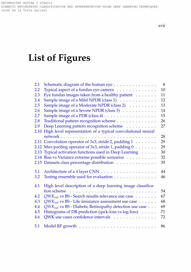
xvii
List of Figures
2.1 Schematic diagram of the human eye . . . . . . . . . . . . . . 82.2 Typical aspect of a fundus eye camera . . . . . . . . . . . . . 102.3 Eye fundus images taken from a healthy patient . . . . . . . 112.4 Sample image of a Mild NPDR (class 1) . . . . . . . . . . . . 122.5 Sample image of a Moderate NPDR (class 2) . . . . . . . . . 132.6 Sample image of a Severe NPDR (class 3) . . . . . . . . . . . 142.7 Sample image of a PDR (class 4) . . . . . . . . . . . . . . . . . 152.8 Traditional pattern recognition scheme . . . . . . . . . . . . . 262.9 Deep Learning pattern recognition scheme . . . . . . . . . . 272.10 High level representation of a typical convolutional neural
network . . . . . . . . . . . . . . . . . . . . . . . . . . . . . . . 282.11 Convolution operator of 3x3, stride 2, padding 1 . . . . . . . 292.12 Max-pooling operator of 3x3, stride 1, padding 0 . . . . . . . 292.13 Typical activation functions used in Deep Learning . . . . . 302.14 Bias vs Variance extreme possible scenarios . . . . . . . . . . 322.15 Datasets class percentage distribution . . . . . . . . . . . . . 35
3.1 Architecture of a 4 layer CNN . . . . . . . . . . . . . . . . . . 443.2 Testing ensemble used for evaluation . . . . . . . . . . . . . . 46
4.1 High level description of a deep learning image classifica-tion scheme . . . . . . . . . . . . . . . . . . . . . . . . . . . . 54
4.2 QWKval vs BS - Search results relevance use case . . . . . . . 674.3 QWKval vs BS - Life insurance assessment use case . . . . . . 684.4 QWKval vs BS - Diabetic Retinopathy detection use case . . . 694.5 Histograms of DR prediction (qwk-loss vs log-loss) . . . . . 714.6 QWK use cases confidence intervals . . . . . . . . . . . . . . 72
5.1 Model RF growth . . . . . . . . . . . . . . . . . . . . . . . . . 86
UNIVERSITAT ROVIRA I VIRGILI DIABETIC RETINOPATHY CLASSIFICATION AND INTERPRETATION USING DEEP LEARNING TECHNIQUES Jordi De la Torre Gallart
xviii
5.2 Feature space cummulative PCA variance of training set . . 875.3 Prediction model . . . . . . . . . . . . . . . . . . . . . . . . . 92
6.1 Hue-Lightness-Saturation color space cone . . . . . . . . . . 956.2 Images used for testing model robustness (Tag: 0) . . . . . . 966.3 Images used for testing model robustness (Tag: 1) . . . . . . 976.4 Images used for testing model robustness (Tag: 2) . . . . . . 986.5 Images used for testing model robustness (Tag: 3) . . . . . . 996.6 Score vs Rotation (Tag: 0) . . . . . . . . . . . . . . . . . . . . . 1036.7 Score vs Rotation (Tag: 1) . . . . . . . . . . . . . . . . . . . . . 1046.8 Score vs Rotation (Tag: 2) . . . . . . . . . . . . . . . . . . . . . 1056.9 Score vs Rotation (Tag: 3) . . . . . . . . . . . . . . . . . . . . . 1066.10 Score vs Lightness (Tag: 0) . . . . . . . . . . . . . . . . . . . . 1076.11 Score vs Lightness (Tag: 1) . . . . . . . . . . . . . . . . . . . . 1086.12 Score vs Lightness (Tag: 2) . . . . . . . . . . . . . . . . . . . . 1096.13 Score vs Lightness (Tag: 3) . . . . . . . . . . . . . . . . . . . . 1106.14 Score vs Saturation (Tag: 0) . . . . . . . . . . . . . . . . . . . 1116.15 Score vs Saturation (Tag: 1) . . . . . . . . . . . . . . . . . . . 1126.16 Score vs Saturation (Tag: 2) . . . . . . . . . . . . . . . . . . . 1136.17 Score vs Saturation (Tag: 3) . . . . . . . . . . . . . . . . . . . 1146.18 Score vs Hue (Tag: 0) . . . . . . . . . . . . . . . . . . . . . . . 1156.19 Score vs Hue (Tag: 1) . . . . . . . . . . . . . . . . . . . . . . . 1166.20 Score vs Hue (Tag: 2) . . . . . . . . . . . . . . . . . . . . . . . 1176.21 Score vs Hue (Tag: 3) . . . . . . . . . . . . . . . . . . . . . . . 118
7.1 Score distribution through layers . . . . . . . . . . . . . . . . 1277.2 Score propagation through an activation function node . . . 1287.3 Score propagation through an batch normalization node . . 1297.4 Convolution score calculation . . . . . . . . . . . . . . . . . . 1307.5 Score propagation through different pooling layers . . . . . . 1307.6 Score propagation through a fully connected node . . . . . . 1317.7 Score propagation through a dropout node . . . . . . . . . . 1327.8 Class 4 sample image . . . . . . . . . . . . . . . . . . . . . . . 1337.9 Class 4 sample intermediate score maps . . . . . . . . . . . . 1347.10 Total score maps . . . . . . . . . . . . . . . . . . . . . . . . . . 136
8.1 Model changes done for improving explainability . . . . . . 142
UNIVERSITAT ROVIRA I VIRGILI DIABETIC RETINOPATHY CLASSIFICATION AND INTERPRETATION USING DEEP LEARNING TECHNIQUES Jordi De la Torre Gallart

xix
8.2 Contribution of each ICA component in the classification fi-nal score . . . . . . . . . . . . . . . . . . . . . . . . . . . . . . 144
8.3 Original and ICA feature space visualization . . . . . . . . . 1468.4 ICA score maps generated for a class 2 image RF 61x61 . . . 1468.5 ICA score maps generated for a class 4 image . . . . . . . . . 1478.6 ICA2 score map for a class 3 image . . . . . . . . . . . . . . . 148
9.1 Feature space visualization of HUSJR dataset . . . . . . . . . 157
UNIVERSITAT ROVIRA I VIRGILI DIABETIC RETINOPATHY CLASSIFICATION AND INTERPRETATION USING DEEP LEARNING TECHNIQUES Jordi De la Torre Gallart

UNIVERSITAT ROVIRA I VIRGILI DIABETIC RETINOPATHY CLASSIFICATION AND INTERPRETATION USING DEEP LEARNING TECHNIQUES Jordi De la Torre Gallart
xxi
List of Tables
2.1 Binary confusion matrix . . . . . . . . . . . . . . . . . . . . . . 162.2 List of the most successful classification architectures used for
Imagenet prediction . . . . . . . . . . . . . . . . . . . . . . . . 31
3.1 Testing scheme performance results . . . . . . . . . . . . . . . 453.2 Frequencies of combined occurrence of classes in both eyes . 473.3 Conditional probabilities of occurrence of DR . . . . . . . . . 473.4 Best classification results for different input sizes . . . . . . . 483.5 Best classification results adding the probabilistic information
of both eyes . . . . . . . . . . . . . . . . . . . . . . . . . . . . . 493.6 Best performing DCNN architecture . . . . . . . . . . . . . . . 50
4.1 Interpretation of Weighted Kappa . . . . . . . . . . . . . . . . 534.2 Search results relevance experiments . . . . . . . . . . . . . . . 744.3 Life insurance assessment experiments . . . . . . . . . . . . . 754.4 DR detection experiments . . . . . . . . . . . . . . . . . . . . . 764.5 Summary of the difference in performance between qwk-loss
and log-loss trained models in function of input size for theDR detection case . . . . . . . . . . . . . . . . . . . . . . . . . . 77
5.1 Prediction performance & model complexity comparison ofour proposal vs the state-of-the-art model (Messidor-2 data set) 90
7.1 Class 4 score map statistics for the analyzed image . . . . . . 135
9.1 CM of HUSJR data using EyePACS trained model . . . . . . . 1579.2 CM of HUSJR data using EyePACS trained model finetuned
with Messidor . . . . . . . . . . . . . . . . . . . . . . . . . . . . 158
UNIVERSITAT ROVIRA I VIRGILI DIABETIC RETINOPATHY CLASSIFICATION AND INTERPRETATION USING DEEP LEARNING TECHNIQUES Jordi De la Torre Gallart

UNIVERSITAT ROVIRA I VIRGILI DIABETIC RETINOPATHY CLASSIFICATION AND INTERPRETATION USING DEEP LEARNING TECHNIQUES Jordi De la Torre Gallart
xxiii
List of Abbreviations
ML Machine LearningDL Deep LearningCNN Convolutional Neural NetworkDCNN Deep Convolutional Neural NetworkBS Batch SizeRF Receptive FieldPCA Principal Components AnalysisICA Independent Components AnalysisIC Independent Component
DM Diabetes MellitusDR Diabetic RetinopathyDME Diabetic Macular EdemaNPDR Non-Proliferative Diabetic RetinopathyPDR Proliferative Diabetic Retinopathy
QWK Quadratic Weighted KappaCM Confusion MatrixTP True PositiveTN True NegativeFP False PositiveFN False NegativeACC AccuracyPPV Positive Predictive ValueNPV Negative Predictive ValueFPR False Positive RateFNR False Negative RateFDR False Discovery RateFOR False Omission Rate
UNIVERSITAT ROVIRA I VIRGILI DIABETIC RETINOPATHY CLASSIFICATION AND INTERPRETATION USING DEEP LEARNING TECHNIQUES Jordi De la Torre Gallart

UNIVERSITAT ROVIRA I VIRGILI DIABETIC RETINOPATHY CLASSIFICATION AND INTERPRETATION USING DEEP LEARNING TECHNIQUES Jordi De la Torre Gallart
xxv
Abstract
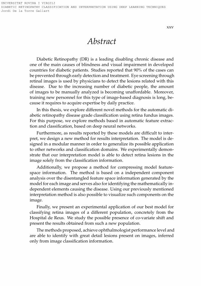
Diabetic Retinopathy (DR) is a leading disabling chronic disease andone of the main causes of blindness and visual impairment in developedcountries for diabetic patients. Studies reported that 90% of the cases canbe prevented through early detection and treatment. Eye screening throughretinal images is used by physicians to detect the lesions related with thisdisease. Due to the increasing number of diabetic people, the amountof images to be manually analyzed is becoming unaffordable. Moreover,training new personnel for this type of image-based diagnosis is long, be-cause it requires to acquire expertise by daily practice.
In this thesis, we explore different novel methods for the automatic di-abetic retinopathy disease grade classification using retina fundus images.For this purpose, we explore methods based in automatic feature extrac-tion and classification, based on deep neural networks.
Furthermore, as results reported by these models are difficult to inter-pret, we design a new method for results interpretation. The model is de-signed in a modular manner in order to generalize its possible applicationto other networks and classification domains. We experimentally demon-strate that our interpretation model is able to detect retina lesions in theimage solely from the classification information.
Additionally, we propose a method for compressing model feature-space information. The method is based on a independent componentanalysis over the disentangled feature space information generated by themodel for each image and serves also for identifying the mathematically in-dependent elements causing the disease. Using our previously mentionedinterpretation method is also possible to visualize such components on theimage.
Finally, we present an experimental application of our best model forclassifying retina images of a different population, concretely from theHospital de Reus. We study the possible presence of co-variate shift andpresent the results obtained from such a new population.
The methods proposed, achieve ophthalmologist performance level andare able to identify with great detail lesions present on images, inferredonly from image classification information.
UNIVERSITAT ROVIRA I VIRGILI DIABETIC RETINOPATHY CLASSIFICATION AND INTERPRETATION USING DEEP LEARNING TECHNIQUES Jordi De la Torre Gallart

xxvi
UNIVERSITAT ROVIRA I VIRGILI DIABETIC RETINOPATHY CLASSIFICATION AND INTERPRETATION USING DEEP LEARNING TECHNIQUES Jordi De la Torre Gallart
1
Chapter 1
Introduction
1.1 Motivation
Computer Science is the field of knowledge that deals with the study ofcomputers and computational systems. Its principal areas include artificialintelligence & machine learning, computer systems & networks, security,databases, human-machine interaction, computer vision, numerical anal-ysis, programming languages, software engineering, bioinformatics andtheory of computing.
Computer vision is an interdisciplinary sub-field of Computer Sciencethat deals with methods for understanding relevant information present inimages. From an engineering perspective, its main purpose is developingmethods and algorithms for automatically acquiring, processing, analyz-ing and understanding images. Typical problems addressed by computervision include image classification, object detection, segmentation, seman-tic segmentation and text explanation generation.
Pattern recognition is a sub-field of Computer Vision which purposeis the design of methods for extracting information from images. It usesmachine learning techniques for extracting the relevant information. Al-though its methods can be generally applied to any signal, a significantpart of the field is devoted to extract infomation from image data.
Medical Imaging is the term used for describing the set of techniquesused for obtaining visual representations of the interior of a body withthe objective of being used for clinical analysis and medical intervention.
UNIVERSITAT ROVIRA I VIRGILI DIABETIC RETINOPATHY CLASSIFICATION AND INTERPRETATION USING DEEP LEARNING TECHNIQUES Jordi De la Torre Gallart
2 Chapter 1. Introduction
It seeks to reveal internal structures hidden inside the body for detect-ing possible pathologies, facilitating diagnosis. Such discipline incorpo-rates radiology, magnetic resonance imaging, medical ultrasonography, en-doscopy, elastography, tactile imaging, thermography, medical photogra-phy and nuclear medicine functional imaging techniques as positron emis-sion tomography (PET) and Single-photon emission computed tomogra-phy (SPECT) (Bushberg and Boone, 2011). Such techniques have been es-sential for improving probability of early detection of many diseases andin this way, reducing also the resources required for treating patients, dueto the fact that early stages of many diseases require milder treatments.
Diabeted melitus (DM) is a chronic disease that affects nearly 400 mil-lion patients worldwide and is expected to increase up to 600 million adultsby 2035 (Aguiree et al., 2013). Spain is expected to have nearly 3 millionDM patients by 2030 (Shaw, Sicree, and Zimmet, 2010). Patients affectedby DM can develop other diseases derived from diabetes. The most seriousDM ocular derived disease is Diabetic Retinopathy (DR). DR is a leadingdisabling chronic disease and one of the main causes of blindness and vi-sual impairment in developed countries for diabetic patients (Fong et al.,2004). Studies reported that 90% of the cases can be prevented throughearly detection and treatment. Eye screening through retinal image anal-ysis is used by physicians to detect lesions related with this disease. Dueto the increasing number of diabetic people, the amount of images to bemanually analyzed is becoming unaffordable. Moreover, training new per-sonnel for this type of image-based diagnosis is long, because it requires toacquire expertise by daily practice. Disease detection using non-mydriaticfundus cameras results to be a very cost effective method for DR screening(Romero-Aroca et al., 2018).
Design of automatic diagnostics systems for Medical Imaging in gen-eral and for DR in particular, could help reducing the prevalence of mostsevere disease cases, increasing the cost effectiveness of diagnostic sys-tems, reducing its associated costs and increasing patients life quality. Themotivation of this thesis is the exploration of new and effective methodsfor the diabetic retinopathy disease detection, classification and lesion de-tection through automatic analysis of retina fundus images.
Traditionally, pattern recognition automatic systems have been basedon the extraction of hand-crafted engineered features or fixed kernels from
UNIVERSITAT ROVIRA I VIRGILI DIABETIC RETINOPATHY CLASSIFICATION AND INTERPRETATION USING DEEP LEARNING TECHNIQUES Jordi De la Torre Gallart
1.2. Objectives 3
the image object of study and the use of a trainable classifier on top ofthem for obtaining the final classification. Using this scheme the problemof the DR detection has been based on hand engineering the features fordetection of disease related lesions, ie. microaneurisms, hemorrhages andexhudates in retinal images that maximize the performance of classifiers.This type of approach requires a good understanding of the disease mecha-nism, requiring a lot of labor time and being very task-specific and therebynot reusable in other classification domains.
In this thesis, we explore a completely different approach consisting onautomatic feature learning. We explore the use deep convolutional neuralnetwork models for predicting disease classification.
1.2 Objectives
The objectives of this thesis are the creation of a human performance leveldiabetic retinopathy automatic classifier using Machine Learning techniquesbased on Deep Learning. The classifier should be able not only of report-ing good classification indexes (near or better than human performance)but also to give additional information to the physicians about the impor-tant elements that the model took into account to arrive to every particularconclusion.
To reach this final objective, we need to achieve other intermediategoals that are described in the following sections. Such intermediate goalsare (1) design a classifier with good balance between performance and re-quired hardware resources, (2) design a method for explaining the resultsreported by the model and finally (3) design a way to express as conciselyas possible the results in order to facilitate the interpretation by humanexperts.
1.2.1 Design of a DR classifier
Deep learning classifier is known to be the best available technique for clas-sification in general applications based on natural images recognition. Atthe beginning of the elaboration of this thesis, deep learning for medicalimaging was in its infancy and it was not clear that such models were able
UNIVERSITAT ROVIRA I VIRGILI DIABETIC RETINOPATHY CLASSIFICATION AND INTERPRETATION USING DEEP LEARNING TECHNIQUES Jordi De la Torre Gallart
4 Chapter 1. Introduction
to evaluate the small lesions present in images and to infer from them astatistically relevant disease classification. Another challenge at the begin-ning of the elaboration of this thesis was the reduced number of availableresources and the limitation of deep learning software libraries. Althoughhaving a big enough public dataset, we did not had enough computationcapability for experimenting with big networks. The first attempts were fo-cused on designing different types of networks, with different input sizes,in order to find the correct balance between size of the network and sizeof the input image, in order to maximize performance. Another challengewas choosing the right minimization function for training the network. Asan ordinal regression problem, the evaluation function used for measuringclassification performance was different from the traditional multi-classclassification loss function, the log-loss. First networks were trained withlog-loss. Afterwards we explored the possibility of directly optimizingsome ordinal based evaluation function, like quadratic weighted kappa.
1.2.2 Design of a system for results interpretation
Deep learning classifiers use to work as black box intuition machines. Whentrained in the right way, they are able to have high statistical confidence butthey do not give any clue of the reasons behind each decision. In medicalimaging, it is critical to be able to explain the reasons behind a conclusion,because part of the curing process can be related with some kind of treat-ment over the disease causal elements. So, our goal for the case of DR dis-ease was helping in the process of lesion location, facilitating an eventualtreatment of surgery over local elements.
1.2.3 Design a model for facilitating the understanding of expla-nations
Machines treat the information in a way different than humans. Comput-ers can handle efficiently multi-dimensional representations. Humans in-terpret data better when presented in reduced dimensional spaces (2D ifpossible). The last objective of the thesis is related with the design of tech-niques for compression representation.
UNIVERSITAT ROVIRA I VIRGILI DIABETIC RETINOPATHY CLASSIFICATION AND INTERPRETATION USING DEEP LEARNING TECHNIQUES Jordi De la Torre Gallart
1.3. Contributions 5
1.3 Contributions
The main contributions of this thesis are:
1. Design of automatic classifiers based on deep neural networks ableto reach ophthalmologist performance level.
Jordi de la Torre, Aïda Valls, and Domenec Puig (2016a). “DiabeticRetinopathy Detection Through Image Analysis Using Deep Convo-lutional Neural Networks”. In: Artificial Intelligence Research and De-velopment - Proceedings of the 19th International Conference of the CatalanAssociation for Artificial Intelligence, Barcelona, Catalonia, Spain, October19-21, 2016. Ed. by Àngela Nebot, Xavier Binefa, and Ramon Lópezde Mántaras. Vol. 288. Frontiers in Artificial Intelligence and Appli-cations. IOS Press, pp. 58–63. ISBN: 978-1-61499-695-8
2. Study of the usage of Quadratic Weighted Kappa index as a DeepLearning Loss Function for the optimization of ordinal regressionproblems.
Jordi de la Torre, Domenec Puig, and Aida Valls (2018). “Weightedkappa loss function for multi-class classification of ordinal data indeep learning”. In: Pattern Recognition Letters 105, pp. 144–154 ImpactFactor: 1.952 (Q2)
3. Design of a generalized model for the interpretation of results re-ported by deep learning classifiers.
Jordi de la Torre, Aida Valls, and Domenec Puig (2017). “A DeepLearning Interpretable Classifier for Diabetic Retinopathy Disease Grad-ing”. In: arXiv preprint arXiv:1712.08107 Accepted for publication inNeurocomputing. Impact Factor: 3.241 (Q1)
4. Design of a method for compressing feature space internal represen-tations of deep learning models.
Jordi de La Torre et al. (2018). “Identification and Visualization ofthe Underlying Independent Causes of the Diagnostic of DiabeticRetinopathy made by a Deep Learning Classifier”. In: CoRR abs/1809.08567.arXiv: 1809.08567. URL: http://arxiv.org/abs/1809.08567
UNIVERSITAT ROVIRA I VIRGILI DIABETIC RETINOPATHY CLASSIFICATION AND INTERPRETATION USING DEEP LEARNING TECHNIQUES Jordi De la Torre Gallart
6 Chapter 1. Introduction
5. Study of the feature space manifold stability of the designed diabeticretinopathy classifiers.
6. Application of designed classifiers into a real use case in Hospital deReus. A software has been implemented for DR classification and le-sion identification. Registered in Benelux Office for Intellectual Prop-erty. Reference number 109999.
1.4 Thesis organization
This thesis is organized as follows: In chapter 1 a brief description of thework motivation is presented. Main contributions done during thesis elab-oration are described and journal publications are cited. In chapter 2 scopeof the work is briefly explained, defining the challenges and tools & tech-niques used for solving them. The following chapters are organized inthree differentiated parts: the first part groups chapters related with Clas-sification (3, 4, 5 and 6), the second part groups chapters related with In-terpretation (chapters 7 and 8) and finally, the third part groups Experimen-tal Applications and Conclusions (chapters 9 and 10). In chapter 3 first de-signed classifiers are presented followed by some ensembling techniquesused for improving results achieved, near human expert performance. Inchapter 4 a new loss function for ordinal regression optimization is pre-sented accompanied with experimental studies validating the increase ofperformance achieved against conventional optimization losses. In chap-ter 5 an improved version of first classifiers is presented, using the newderived loss function and other changes, achieving ophthalmologist levelperformance. In chapter 6 a feature-space manifold stability study is alsopresented for evaluation of the stability of the model internal representa-tion to changes in input structure. In chapter 7 a general interpretationmodel for deep learning classifiers is presented and applied to the specificcase of our diabetic retinopathy classifiers achieving an excellent perfor-mance in lesion detection. In chapter 8 a system for feature-space com-pression is presented. In chapter 9 a research results case study applicationis presented, applying the classifiers for prediction of Hospital UniversitariSant Joan de Reus population. A set of studies for evaluation of covariateshift of training and new test set population are also presented. Finally, inchapter 10 thesis conclusions and future work directions are described.
UNIVERSITAT ROVIRA I VIRGILI DIABETIC RETINOPATHY CLASSIFICATION AND INTERPRETATION USING DEEP LEARNING TECHNIQUES Jordi De la Torre Gallart
7
Chapter 2
Background
2.1 Diabetic retinopathy
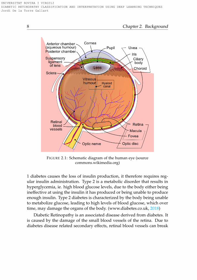
Eyes are globular organs of sight present in humans and vertebrates withthe function of capturing the light coming from the environment and con-vert it into signals that are interpreted by the brain as images. From thisimages the brain is able to extract information and construct abstractionsfrom the external world. Eyes are composed of different parts, each onehaving a differentiated function (see figure 2.1). Light coming from theenvironment travels through the cornea, iris and lens, reaching the retina,situated in the internal back side of the eyeball. Retina is continuous withthe optic nerve, and consists of several layers, one of which contains therods and cones that are sensitive to light. Activated rods and cones trans-fer information through the optic nerve, that is interpreted by the brain asan image.
Diabetes is a disorder of the body due to its inability of producing orresponding to the hormone insulin, resulting in abnormal metabolism ofcarbohydrates and elevated levels of glucose in the blood. Such high bloodglucose levels can damage blood vessels and nerves, increasing the prob-ability in diabetic patients of developing other derived diseases, like Dia-betic Retinopathy.
Diabetes can be of two different types: type 1 and 2. Type 1 is an au-toimmune disease that causes the insulin producing beta cells in the pan-creas to be destroyed, preventing the body from being able to produceenough insulin to adequately regulate blood glucose levels. Because type
UNIVERSITAT ROVIRA I VIRGILI DIABETIC RETINOPATHY CLASSIFICATION AND INTERPRETATION USING DEEP LEARNING TECHNIQUES Jordi De la Torre Gallart
8 Chapter 2. Background
FIGURE 2.1: Schematic diagram of the human eye (sourcecommons.wikimedia.org)
1 diabetes causes the loss of insulin production, it therefore requires reg-ular insulin administration. Type 2 is a metabolic disorder that results inhyperglycemia, ie. high blood glucose levels, due to the body either beingineffective at using the insulin it has produced or being unable to produceenough insulin. Type 2 diabetes is characterized by the body being unableto metabolize glucose, leading to high levels of blood glucose, which overtime, may damage the organs of the body. (www.diabetes.co.uk, 2018)
Diabetic Retinopathy is an associated disease derived from diabetes. Itis caused by the damage of the small blood vessels of the retina. Due todiabetes disease related secondary effects, retinal blood vessels can break
UNIVERSITAT ROVIRA I VIRGILI DIABETIC RETINOPATHY CLASSIFICATION AND INTERPRETATION USING DEEP LEARNING TECHNIQUES Jordi De la Torre Gallart
2.1. Diabetic retinopathy 9
down, leak or become blocked; affecting the transport of nutrients and oxy-gen to parts of the retina, causing impaired vision over time. Due to theblockages, abnormal blood vessels can grow on the retina surface, caus-ing an increment of the probability of bleeding and liquid leakages. Suchstructural changes can result initially in vision blurring and in last stages,even in retinal detachment and/or glaucoma.
During the first two decades of the diabetes disease, nearly all patientswith type 1 and more than 60% of patients with type 2 diabetes, will de-velop a retinopathy (Fong et al., 2004).
2.1.1 Retina health evaluation
There are several tests that a doctor may perform to evaluate retina eyehealth:
An ophtalmoscope is a specialized type of microscope that allows theinspection of the vitreus, retina and other internal structures of the eye.With this instrument is possible to create a mirrored image of the variousportions of the eye.
A visual field or perimetry test, mesures the ability of the examined eyeto see straight ahead and the peripheral vision. The purpose of this testis to determine if there are any peripheral vision areas that are developingblind spots.
Fluorescein angiography allows the doctor to inspect retina blood vessels.A vegetable-based dye is injected into patient blood stream. As blood cir-culates in the retina, a series of quick, sequential photographs of the eye aretaken. These photographs provide useful information about its condition.Fluorescein angiography is one of the most important tests performed fordetermining the diagnosis and treatment of retinal disorders.
B-scan ultrasound uses high frequency sound waves to view the backportions of the eye. This technology provides a full surface view of the eyethat can be also used for retina condition evaluation.
Fundus photography utilizes special cameras to document and track theprogress of certain retinal diseases, like diabetic retinopathy, as well asmonitor its treatment. This type of images are the used in this thesis forcreating the automatic diagnostic system.
UNIVERSITAT ROVIRA I VIRGILI DIABETIC RETINOPATHY CLASSIFICATION AND INTERPRETATION USING DEEP LEARNING TECHNIQUES Jordi De la Torre Gallart
10 Chapter 2. Background
Fundus photography
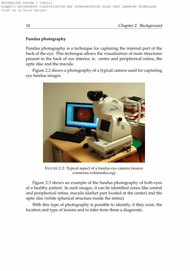
Fundus photography is a technique for capturing the internal part of theback of the eye. This technique allows the visualization of main structurespresent in the back of eye interior, ie. center and peripherical retina, theoptic disc and the macula.
Figure 2.2 shows a photography of a typical camera used for capturingeye fundus images.
FIGURE 2.2: Typical aspect of a fundus eye camera (sourcecommons.wikimedia.org)
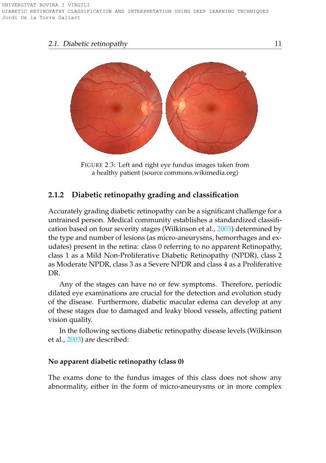
Figure 2.3 shows an example of the fundus photography of both eyesof a healthy patient. In such images, it can be identified zones like centraland peripherical retina, macula (darker part located at the center) and theoptic disc (white spherical structure inside the retina).
With this type of photography is possible to identify, if they exist, thelocation and type of lesions and to infer from them a diagnostic.
UNIVERSITAT ROVIRA I VIRGILI DIABETIC RETINOPATHY CLASSIFICATION AND INTERPRETATION USING DEEP LEARNING TECHNIQUES Jordi De la Torre Gallart
2.1. Diabetic retinopathy 11
FIGURE 2.3: Left and right eye fundus images taken froma healthy patient (source commons.wikimedia.org)
2.1.2 Diabetic retinopathy grading and classification
Accurately grading diabetic retinopathy can be a significant challenge for auntrained person. Medical community establishes a standardized classifi-cation based on four severity stages (Wilkinson et al., 2003) determined bythe type and number of lesions (as micro-aneurysms, hemorrhages and ex-udates) present in the retina: class 0 referring to no apparent Retinopathy,class 1 as a Mild Non-Proliferative Diabetic Retinopathy (NPDR), class 2as Moderate NPDR, class 3 as a Severe NPDR and class 4 as a ProliferativeDR.
Any of the stages can have no or few symptoms. Therefore, periodicdilated eye examinations are crucial for the detection and evolution studyof the disease. Furthermore, diabetic macular edema can develop at anyof these stages due to damaged and leaky blood vessels, affecting patientvision quality.
In the following sections diabetic retinopathy disease levels (Wilkinsonet al., 2003) are described:
No apparent diabetic retinopathy (class 0)
The exams done to the fundus images of this class does not show anyabnormality, either in the form of micro-aneurysms or in more complex
UNIVERSITAT ROVIRA I VIRGILI DIABETIC RETINOPATHY CLASSIFICATION AND INTERPRETATION USING DEEP LEARNING TECHNIQUES Jordi De la Torre Gallart
12 Chapter 2. Background
forms. A diabetic patient with no retinopathy has a < 1% chance of devel-oping a PDR in the next four years (Klein et al., 2009).
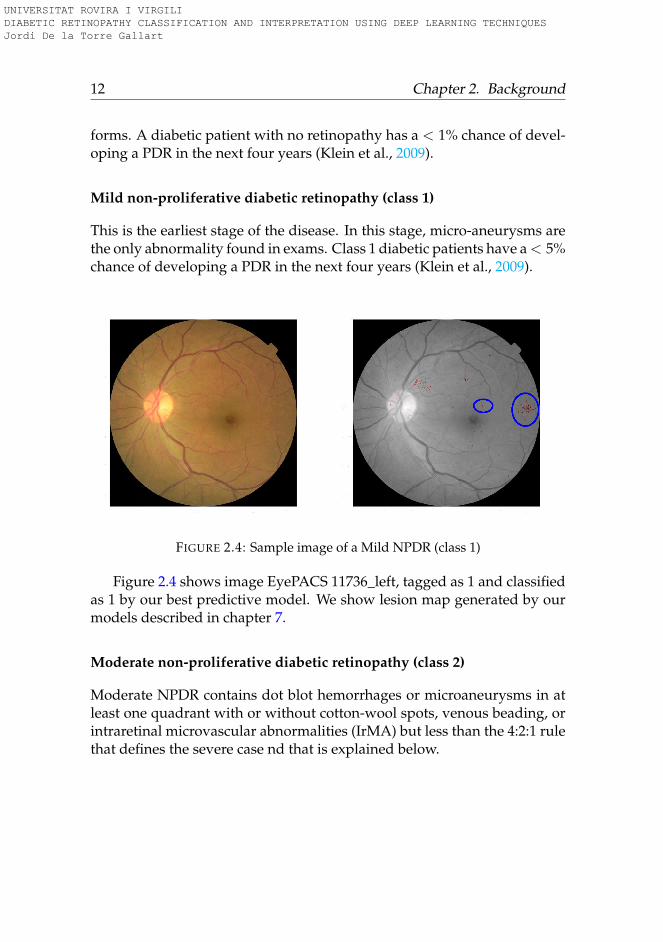
Mild non-proliferative diabetic retinopathy (class 1)
This is the earliest stage of the disease. In this stage, micro-aneurysms arethe only abnormality found in exams. Class 1 diabetic patients have a < 5%chance of developing a PDR in the next four years (Klein et al., 2009).
FIGURE 2.4: Sample image of a Mild NPDR (class 1)
Figure 2.4 shows image EyePACS 11736_left, tagged as 1 and classifiedas 1 by our best predictive model. We show lesion map generated by ourmodels described in chapter 7.
Moderate non-proliferative diabetic retinopathy (class 2)
Moderate NPDR contains dot blot hemorrhages or microaneurysms in atleast one quadrant with or without cotton-wool spots, venous beading, orintraretinal microvascular abnormalities (IrMA) but less than the 4:2:1 rulethat defines the severe case nd that is explained below.
UNIVERSITAT ROVIRA I VIRGILI DIABETIC RETINOPATHY CLASSIFICATION AND INTERPRETATION USING DEEP LEARNING TECHNIQUES Jordi De la Torre Gallart
2.1. Diabetic retinopathy 13
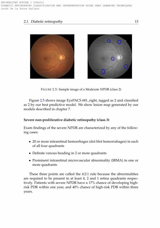
FIGURE 2.5: Sample image of a Moderate NPDR (class 2)
Figure 2.5 shows image EyePACS 681_right, tagged as 2 and classifiedas 2 by our best predictive model. We show lesion map generated by ourmodels described in chapter 7.
Severe non-proliferative diabetic retinopathy (class 3)
Exam findings of the severe NPDR are characterized by any of the follow-ing cases:
• 20 or more intraretinal hemorrhages (dot blot hemorrahages) in eachof all four quadrants
• Definite venous beading in 2 or more quadrants
• Prominent intraretinal microvascular abnormality (IRMA) in one ormore quadrants
These three points are called the 4:2:1 rule because the abnormalitiesare required to be present in at least 4, 2 and 1 retina quadrants respec-tively. Patients with severe NPDR have a 17% chance of developing high-risk PDR within one year, and 40% chance of high-risk PDR within threeyears.
UNIVERSITAT ROVIRA I VIRGILI DIABETIC RETINOPATHY CLASSIFICATION AND INTERPRETATION USING DEEP LEARNING TECHNIQUES Jordi De la Torre Gallart
14 Chapter 2. Background
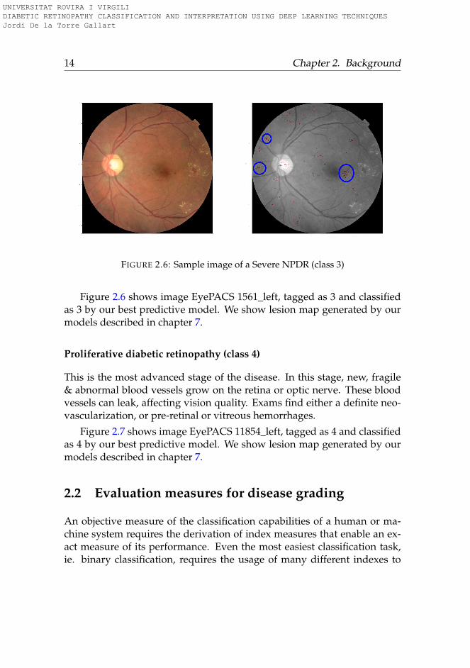
FIGURE 2.6: Sample image of a Severe NPDR (class 3)
Figure 2.6 shows image EyePACS 1561_left, tagged as 3 and classifiedas 3 by our best predictive model. We show lesion map generated by ourmodels described in chapter 7.
Proliferative diabetic retinopathy (class 4)
This is the most advanced stage of the disease. In this stage, new, fragile& abnormal blood vessels grow on the retina or optic nerve. These bloodvessels can leak, affecting vision quality. Exams find either a definite neo-vascularization, or pre-retinal or vitreous hemorrhages.
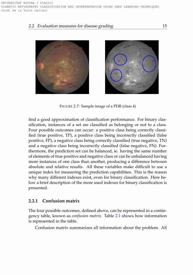
Figure 2.7 shows image EyePACS 11854_left, tagged as 4 and classifiedas 4 by our best predictive model. We show lesion map generated by ourmodels described in chapter 7.
2.2 Evaluation measures for disease grading
An objective measure of the classification capabilities of a human or ma-chine system requires the derivation of index measures that enable an ex-act measure of its performance. Even the most easiest classification task,ie. binary classification, requires the usage of many different indexes to
UNIVERSITAT ROVIRA I VIRGILI DIABETIC RETINOPATHY CLASSIFICATION AND INTERPRETATION USING DEEP LEARNING TECHNIQUES Jordi De la Torre Gallart
2.2. Evaluation measures for disease grading 15
FIGURE 2.7: Sample image of a PDR (class 4)
find a good approximation of classification performance. For binary clas-sification, instances of a set are classified as belonging or not to a class.Four possible outcomes can occur: a positive class being correctly classi-fied (true positive, TP), a positive class being incorrectly classified (falsepositive, FP), a negative class being correctly classified (true negative, TN)and a negative class being incorrectly classified (false negative, FN). Fur-thermore, the prediction set can be balanced, ie. having the same numberof elements of true positive and negative class or can be unbalanced havingmore instances of one class than another, producing a difference betweenabsolute and relative results. All these variables make difficult to use aunique index for measuring the prediction capabilities. This is the reasonwhy many different indexes exist, even for binary classification. Here be-low a brief description of the more used indexes for binary classification ispresented.
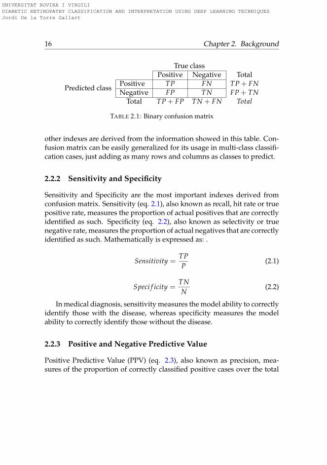
2.2.1 Confusion matrix
The four possible outcomes, defined above, can be represented in a contin-gency table, known as confusion matrix. Table 2.1 shows how informationis represented in the table.
Confusion matrix summarizes all information about the problem. All
UNIVERSITAT ROVIRA I VIRGILI DIABETIC RETINOPATHY CLASSIFICATION AND INTERPRETATION USING DEEP LEARNING TECHNIQUES Jordi De la Torre Gallart
16 Chapter 2. Background
True classPositive Negative Total
Predicted classPositive TP FN TP + FNNegative FP TN FP + TN
Total TP + FP TN + FN Total
TABLE 2.1: Binary confusion matrix
other indexes are derived from the information showed in this table. Con-fusion matrix can be easily generalized for its usage in multi-class classifi-cation cases, just adding as many rows and columns as classes to predict.
2.2.2 Sensitivity and Specificity
Sensitivity and Specificity are the most important indexes derived fromconfusion matrix. Sensitivity (eq. 2.1), also known as recall, hit rate or truepositive rate, measures the proportion of actual positives that are correctlyidentified as such. Specificity (eq. 2.2), also known as selectivity or truenegative rate, measures the proportion of actual negatives that are correctlyidentified as such. Mathematically is expressed as: .
Sensitivity =TPP
(2.1)
Speci f icity =TNN
(2.2)
In medical diagnosis, sensitivity measures the model ability to correctlyidentify those with the disease, whereas specificity measures the modelability to correctly identify those without the disease.
2.2.3 Positive and Negative Predictive Value
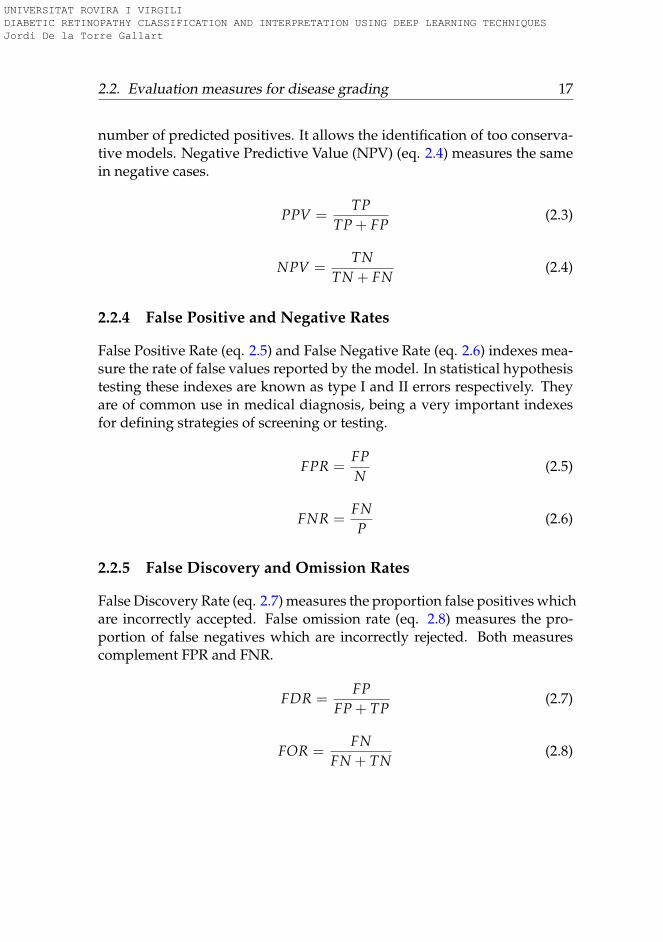
Positive Predictive Value (PPV) (eq. 2.3), also known as precision, mea-sures of the proportion of correctly classified positive cases over the total
UNIVERSITAT ROVIRA I VIRGILI DIABETIC RETINOPATHY CLASSIFICATION AND INTERPRETATION USING DEEP LEARNING TECHNIQUES Jordi De la Torre Gallart
2.2. Evaluation measures for disease grading 17
number of predicted positives. It allows the identification of too conserva-tive models. Negative Predictive Value (NPV) (eq. 2.4) measures the samein negative cases.
PPV =TP
TP + FP(2.3)
NPV =TN
TN + FN(2.4)
2.2.4 False Positive and Negative Rates
False Positive Rate (eq. 2.5) and False Negative Rate (eq. 2.6) indexes mea-sure the rate of false values reported by the model. In statistical hypothesistesting these indexes are known as type I and II errors respectively. Theyare of common use in medical diagnosis, being a very important indexesfor defining strategies of screening or testing.
FPR =FPN
(2.5)
FNR =FNP
(2.6)
2.2.5 False Discovery and Omission Rates
False Discovery Rate (eq. 2.7) measures the proportion false positives whichare incorrectly accepted. False omission rate (eq. 2.8) measures the pro-portion of false negatives which are incorrectly rejected. Both measurescomplement FPR and FNR.
FDR =FP
FP + TP(2.7)
FOR =FN
FN + TN(2.8)
UNIVERSITAT ROVIRA I VIRGILI DIABETIC RETINOPATHY CLASSIFICATION AND INTERPRETATION USING DEEP LEARNING TECHNIQUES Jordi De la Torre Gallart
18 Chapter 2. Background
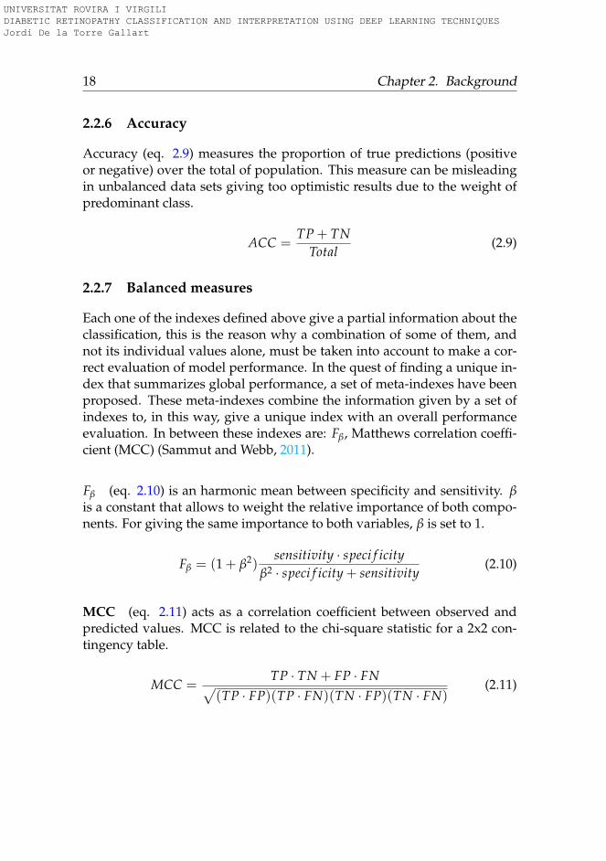
2.2.6 Accuracy
Accuracy (eq. 2.9) measures the proportion of true predictions (positiveor negative) over the total of population. This measure can be misleadingin unbalanced data sets giving too optimistic results due to the weight ofpredominant class.
ACC =TP + TN
Total(2.9)
2.2.7 Balanced measures
Each one of the indexes defined above give a partial information about theclassification, this is the reason why a combination of some of them, andnot its individual values alone, must be taken into account to make a cor-rect evaluation of model performance. In the quest of finding a unique in-dex that summarizes global performance, a set of meta-indexes have beenproposed. These meta-indexes combine the information given by a set ofindexes to, in this way, give a unique index with an overall performanceevaluation. In between these indexes are: Fβ, Matthews correlation coeffi-cient (MCC) (Sammut and Webb, 2011).
Fβ (eq. 2.10) is an harmonic mean between specificity and sensitivity. βis a constant that allows to weight the relative importance of both compo-nents. For giving the same importance to both variables, β is set to 1.
Fβ = (1 + β2)sensitivity · speci f icity
β2 · speci f icity + sensitivity(2.10)
MCC (eq. 2.11) acts as a correlation coefficient between observed andpredicted values. MCC is related to the chi-square statistic for a 2x2 con-tingency table.
MCC =TP · TN + FP · FN√
(TP · FP)(TP · FN)(TN · FP)(TN · FN)(2.11)
UNIVERSITAT ROVIRA I VIRGILI DIABETIC RETINOPATHY CLASSIFICATION AND INTERPRETATION USING DEEP LEARNING TECHNIQUES Jordi De la Torre Gallart
2.2. Evaluation measures for disease grading 19
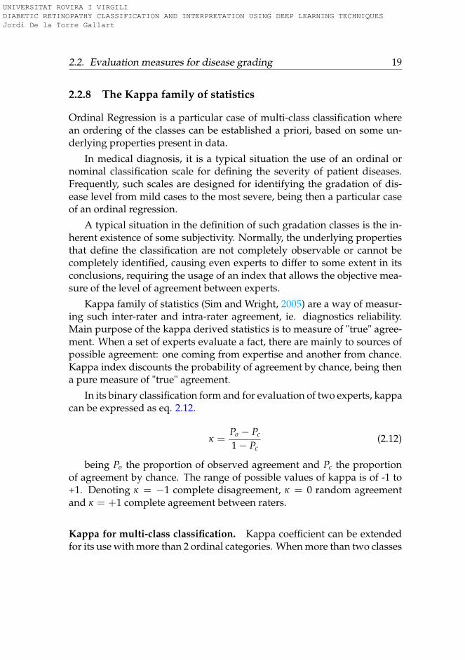
2.2.8 The Kappa family of statistics
Ordinal Regression is a particular case of multi-class classification wherean ordering of the classes can be established a priori, based on some un-derlying properties present in data.
In medical diagnosis, it is a typical situation the use of an ordinal ornominal classification scale for defining the severity of patient diseases.Frequently, such scales are designed for identifying the gradation of dis-ease level from mild cases to the most severe, being then a particular caseof an ordinal regression.
A typical situation in the definition of such gradation classes is the in-herent existence of some subjectivity. Normally, the underlying propertiesthat define the classification are not completely observable or cannot becompletely identified, causing even experts to differ to some extent in itsconclusions, requiring the usage of an index that allows the objective mea-sure of the level of agreement between experts.
Kappa family of statistics (Sim and Wright, 2005) are a way of measur-ing such inter-rater and intra-rater agreement, ie. diagnostics reliability.Main purpose of the kappa derived statistics is to measure of "true" agree-ment. When a set of experts evaluate a fact, there are mainly to sources ofpossible agreement: one coming from expertise and another from chance.Kappa index discounts the probability of agreement by chance, being thena pure measure of "true" agreement.
In its binary classification form and for evaluation of two experts, kappacan be expressed as eq. 2.12.
κ =Po − Pc
1− Pc(2.12)
being Po the proportion of observed agreement and Pc the proportionof agreement by chance. The range of possible values of kappa is of -1 to+1. Denoting κ = −1 complete disagreement, κ = 0 random agreementand κ = +1 complete agreement between raters.
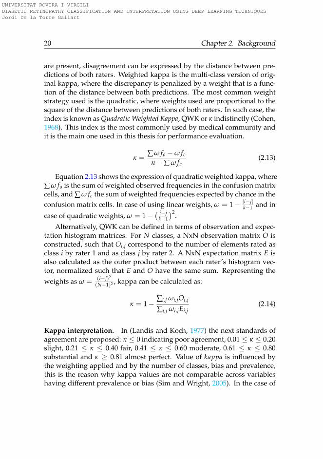
Kappa for multi-class classification. Kappa coefficient can be extendedfor its use with more than 2 ordinal categories. When more than two classes
UNIVERSITAT ROVIRA I VIRGILI DIABETIC RETINOPATHY CLASSIFICATION AND INTERPRETATION USING DEEP LEARNING TECHNIQUES Jordi De la Torre Gallart
20 Chapter 2. Background
are present, disagreement can be expressed by the distance between pre-dictions of both raters. Weighted kappa is the multi-class version of orig-inal kappa, where the discrepancy is penalized by a weight that is a func-tion of the distance between both predictions. The most common weightstrategy used is the quadratic, where weights used are proportional to thesquare of the distance between predictions of both raters. In such case, theindex is known as Quadratic Weighted Kappa, QWK or κ indistinctly (Cohen,1968). This index is the most commonly used by medical community andit is the main one used in this thesis for performance evaluation.
κ =∑ ω fo −ω fc
n−∑ ω fc(2.13)
Equation 2.13 shows the expression of quadratic weighted kappa, where∑ ω fo is the sum of weighted observed frequencies in the confusion matrixcells, and ∑ ω fc the sum of weighted frequencies expected by chance in theconfusion matrix cells. In case of using linear weights, ω = 1− |i−j|
k−1 and in
case of quadratic weights, ω = 1−( i−j
k−1
)2.
Alternatively, QWK can be defined in terms of observation and expec-tation histogram matrices. For N classes, a NxN observation matrix O isconstructed, such that Oi,j correspond to the number of elements rated asclass i by rater 1 and as class j by rater 2. A NxN expectation matrix E isalso calculated as the outer product between each rater’s histogram vec-tor, normalized such that E and O have the same sum. Representing theweights as ω = (i−j)2
(N−1)2 , kappa can be calculated as:
κ = 1− ∑i,j ωi,jOi,j
∑i,j ωi,jEi,j(2.14)
Kappa interpretation. In (Landis and Koch, 1977) the next standards ofagreement are proposed: κ ≤ 0 indicating poor agreement, 0.01 ≤ κ ≤ 0.20slight, 0.21 ≤ κ ≤ 0.40 fair, 0.41 ≤ κ ≤ 0.60 moderate, 0.61 ≤ κ ≤ 0.80substantial and κ ≥ 0.81 almost perfect. Value of kappa is influenced bythe weighting applied and by the number of classes, bias and prevalence,this is the reason why kappa values are not comparable across variableshaving different prevalence or bias (Sim and Wright, 2005). In the case of
UNIVERSITAT ROVIRA I VIRGILI DIABETIC RETINOPATHY CLASSIFICATION AND INTERPRETATION USING DEEP LEARNING TECHNIQUES Jordi De la Torre Gallart
2.3. Machine Learning 21
diabetic retinopathy disease grading, using QWK, the inter-rating agree-ment between expert ophthalmologists is about 0.80. For the purpose ofthis thesis, such value (κ = 0.80) is the standard of reference our modelsare compared against.
2.2.9 How to define human performance
A key factor for evaluation of machine performance against humans is thestandard used to measure the last one. In the context of medical classifica-tion, the next comparison standards can be used:
1. A person (not a doctor)
2. A general doctor
3. A specialized doctor
4. A highly experienced specialized doctor
5. A team of highly experienced specialized doctors
The team of highly experienced specialized doctors can be approxi-mated to the Bayes Optimal Error (Fukunaga, 2013), (Tumer and Ghosh,1996). In any case, it is important to define the standard we are comparingagainst. For the purpose of this thesis, human performance is establishedas the given by a highly experienced specialized doctor.
2.3 Machine Learning
Machine Learning is a Computer Science discipline, sub-field of ArtificialIntelligence, that include all the tools and techniques used for enablingcomputers to learn from data and, from a more ambitious perspective, giv-ing computers the ability of acting without being explicitly programmed.
All tools and techniques available in the discipline can be classified ac-cording on the type of learning algorithm that they implement: supervised,unsupervised and reinforced learning.
UNIVERSITAT ROVIRA I VIRGILI DIABETIC RETINOPATHY CLASSIFICATION AND INTERPRETATION USING DEEP LEARNING TECHNIQUES Jordi De la Torre Gallart
22 Chapter 2. Background
Supervised learning algorithms require all the instances of the trainingset to be labeled. From this previous knowledge the algorithm is able tolearn and generalize, being able to predict new never seen before samples.From a probability perspective these type of algorithms learn a conditionaldistribution, ie. P(c|X), being c the class to predict and X the sample.
Unsupervised learning algorithms allow the learning of underlying reg-ularities present in the training set without requiring labeling of the indi-vidual instances. From a probability perspective, such models are able tolearn the joint distribution of the population represented by the trainingset, ie. P(X), being X the sample.
Reinforcement learning algorithms give models the capacity of learningfrom environment, ie. accumulating experience from its interaction withthe surroundings. Such models are goal oriented, having an internal rep-resentation of the environment that is updated periodically with the objec-tive of maximizing gain.
2.3.1 Supervised Learning
In this thesis we used supervised learning techniques for learning fromdata. As previously stated, in this learning paradigm a labeled training setis used as a foundation for learning general representations that can beused for generalizing behaviors and inferring then new labels in never seenbefore data.
Classification vs Regression
The objective of supervised learning is the learning of a conditional prob-ability distribution in the form of P(c|X). Depending on the nature of thevariable to be predicted, it can be differentiated between classification orregression. Fundamentally, classification is about a disjoint class label pre-diction and regression is about a quantity prediction. Ordinal regression isa particular case of classification, where some a priori class ordinality canbe established.
UNIVERSITAT ROVIRA I VIRGILI DIABETIC RETINOPATHY CLASSIFICATION AND INTERPRETATION USING DEEP LEARNING TECHNIQUES Jordi De la Torre Gallart
2.3. Machine Learning 23
Dataset management
In supervised learning, the source of knowledge is represented by a labeleddata set. The probability distribution of the population that it is supposedto be predicted is assumed to be represented by a sample, ie. a labeled dataset. The design process of a predictive model has two parts: building themodel (ie. training) and statistical evaluation of its performance. Perfor-mance evaluation require the usage of a never seen before data set, so theoriginal full data set is required to be split in two parts: one for training(called training set) and another for testing (called test set). Both train andtest set must be big enough either for training good models or for having ahigh statistical confidence of its generalization capabilities.
Strategies for hyper-parameter optimization
Frequently, supervised learning models have parameters that must be fixedbefore learning. In such cases, model performance can change dramaticallydepending on the selected parameters, requiring also a meta-learning pa-rameter optimization for selection of the highest performance model, morecommonly known as hyper-parameter optimization.
Different strategies can be followed in order to optimize such meta-parameters:
Hold Out method: This method splits original training data set usingrandom sampling without repetition into 2 subsets. The first called train-ing set is used for fitting the model/s, the second one, called validation setis used for hyper-parameter optimization and for model selection, not onlybetween hyper-parameters but also between different types of models. Asa rule of thumb, training set use to have between 50% to 70% of the dataand validation set between 50% to 30%.
K-fold cross validation: The original training set is split in K folds of thesame size using random sampling without repetition. The model/s aretrained K times, each one of them using as training set K − 1 folds and 1(the not used one) as a validation set. Prediction error is the average ofK individual errors. Error variance can be used as a measure of the model
UNIVERSITAT ROVIRA I VIRGILI DIABETIC RETINOPATHY CLASSIFICATION AND INTERPRETATION USING DEEP LEARNING TECHNIQUES Jordi De la Torre Gallart
24 Chapter 2. Background
stability. The advantage of this method is that it matters less how the data isdivided, ie. the model is less prone of having selection bias. After choosingthe best model hyper-parameters and/or model, a retrain with the wholedata set is recommended.
Leave one out cross-validation: It is a type of K-fold cross validationwhere it is hold out only one sample each time. It is a good way to val-idate, but requires a high computation time.
Bootstrap methods: It randomly draws data sets from the original sam-ple. Each sample size is equal to the original training size. Each model/swith its particular hyper-parameters is fitted using the bootstrapped sam-ples. Model/s are examined with the out-of-bag data, ie. data not selectedin each bootstrap.
2.3.2 Algorithms used in supervised machine learning
The most widely used learning algorithms can be divided into the nextcategories:
• Linear / Logistic regression
• Support Vector Machines
• Probabilistic Graphical Models
• Decision trees related algorithms
• Deep Learning (Multilayer Perceptron, Neural Networks)
• Others (clustering, association rules, inductive logic, representationlearning, similarity and metric learning, sparse dictionary learning,genetic algorithms, etc.)
Linear/Logistic Regression are regression and classification algorithms,where a linear combination of the inputs is optimized for least squares er-ror minimization in the first case and for cross entropy minimization in thesecond.
UNIVERSITAT ROVIRA I VIRGILI DIABETIC RETINOPATHY CLASSIFICATION AND INTERPRETATION USING DEEP LEARNING TECHNIQUES Jordi De la Torre Gallart
2.3. Machine Learning 25
Support Vector Machines are similar to linear/logistic regression but us-ing a different optimization function. They minimize the Hinge loss, givingas a result maximum-margin classifiers. Support vector machines can beused as linear classifiers but also as a non-linear ones, substituting its fea-tures with so-called kernels, that are non-linear functions of the featuresand training set samples.
Probabilistic Graphical Models are a set of models based on probabilis-tic conditional dependency graphs that use bayesian rules for model con-struction and inference.
Decision Trees based models are a set of very effective algorithms basedon the usage of weak learners like decision trees for constructing very pow-erful predictors combining them using bagging or boosting techniques.This category include algorithms like Random Forest or Gradient Boost-ing.
Deep Learning also known as Artificial Neural Networks or MultilayerPerceptrons, is a set of Machine Learning techniques for automatically con-structing models from the underlying distribution represented by a largeset of examples, using multiple levels of representation (in the form oflayers), with the final objective of mapping a high-multidimensional in-put into a smaller multidimensional output (f: Rn 7→ Rm, n � m). Thismapping allows the classification of multidimensional objects into a smallnumber of categories. The model is composed by many neurons that areorganized in layers and blocks of layers, using a cascade of layers in a hier-archical way. Every neuron receives the input from a predefined set of neu-rons. Every connection has a parameter that corresponds to the weight ofthe connection. The function of every neuron is to make a transformationof the received inputs into a calculated output value. For every incom-ing connection, the weight is multiplied by the input value received bythe neuron and the aggregated value that used by an activation functionthat calculates the output of the neuron. Parameters are usually optimizedusing a stochastic gradient descent algorithm that minimizes a predefinedloss function. Network parameters are updated after back-propagating theloss function gradients through the network. These hierarchical models are
UNIVERSITAT ROVIRA I VIRGILI DIABETIC RETINOPATHY CLASSIFICATION AND INTERPRETATION USING DEEP LEARNING TECHNIQUES Jordi De la Torre Gallart
26 Chapter 2. Background
able to learn multiple levels of representation that correspond to differentlevels of abstraction, which enables the representation of complex conceptsin a compressed way (Lecun, Bengio, and Hinton, 2015), (Schmidhuber,2015), (Bengio, Courville, and Vincent, 2013), (Bengio, 2009). The modelsused in this thesis are based mainly in Deep Learning.
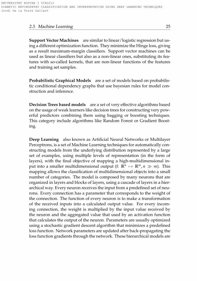
2.3.3 Pattern recognition
Traditional models of pattern recognition
The traditional model for pattern recognition since the 50’s were based ona fix design of a set of important features manually engineered or derivedfrom a fixed kernel (Fig. 2.8). Such kernels allowed the extraction of tex-ture, statistic, position, geometry features that were posteriously combinedwith a simple classifier. A great diversity of methods for feature extrac-tion exist as the local binary pattern, histogram of oriented gradients, graylevel co-occurence matrix, gabor filters, between others. In the classifica-tion phase it was common practice to use k-nearest neighbors, linear dis-criminant analysis, support vector machines or decision trees derived al-gorithms like random forest or gradient boosting.
ImageInput
Hand-CraftedFeature
Extractor
’Simple’Classifier Class
FIGURE 2.8: Traditional pattern recognition scheme
Such pattern recognition pipeline required a lot of labor time for de-signing the appropriate filters for every particular application.
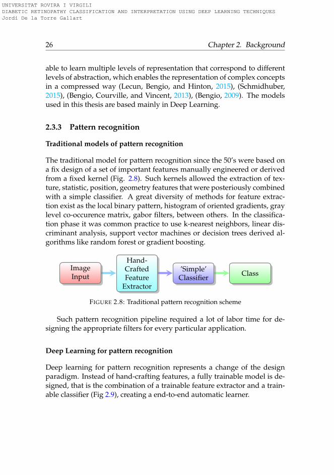
Deep Learning for pattern recognition
Deep learning for pattern recognition represents a change of the designparadigm. Instead of hand-crafting features, a fully trainable model is de-signed, that is the combination of a trainable feature extractor and a train-able classifier (Fig 2.9), creating a end-to-end automatic learner.
UNIVERSITAT ROVIRA I VIRGILI DIABETIC RETINOPATHY CLASSIFICATION AND INTERPRETATION USING DEEP LEARNING TECHNIQUES Jordi De la Torre Gallart
2.3. Machine Learning 27
ImageInput
TrainableFeature
Extractor
TrainableClassifier Class
FIGURE 2.9: Deep Learning pattern recognition scheme(end-to-end learning)
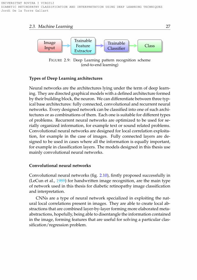
Types of Deep Learning architectures
Neural networks are the architectures lying under the term of deep learn-ing. They are directed graphical models with a defined architecture formedby their building block, the neuron. We can differentiate between three typ-ical base architectures: fully connected, convolutional and recurrent neuralnetworks. Every designed network can be classified into one of such archi-tectures or as combinations of them. Each one is suitable for different typesof problems. Recurrent neural networks are optimized to be used for se-rially organized information, for example text or sound related problems.Convolutional neural networks are designed for local correlation exploita-tion, for example in the case of images. Fully connected layers are de-signed to be used in cases where all the information is equally important,for example in classification layers. The models designed in this thesis usemainly convolutional neural networks.
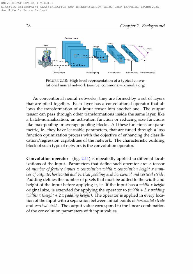
Convolutional neural networks
Convolutional neural networks (fig. 2.10), firstly proposed successfully in(LeCun et al., 1989) for handwritten image recognition, are the main typeof network used in this thesis for diabetic retinopathy image classificationand interpretation.
CNNs are a type of neural network specialized in exploiting the nat-ural local correlations present in images. They are able to create local ab-stractions that are combined layer-by-layer forming more elaborated meta-abstractions, hopefully, being able to disentangle the information containedin the image, forming features that are useful for solving a particular clas-sification/regression problem.
UNIVERSITAT ROVIRA I VIRGILI DIABETIC RETINOPATHY CLASSIFICATION AND INTERPRETATION USING DEEP LEARNING TECHNIQUES Jordi De la Torre Gallart
28 Chapter 2. Background
FIGURE 2.10: High level representation of a typical convo-lutional neural network (source: commons.wikimedia.org)
As conventional neural networks, they are formed by a set of layersthat are piled together. Each layer has a convolutional operator that al-lows the transformation of a input tensor into another one. The outputtensor can pass through other transformations inside the same layer, likea batch-normalization, an activation function or reducing size functionslike max-pooling or average pooling blocks. All these functions are para-metric, ie. they have learnable parameters, that are tuned through a lossfunction optimization process with the objective of enhancing the classifi-cation/regression capabilities of the network. The characteristic buildingblock of such type of network is the convolution operator.
Convolution operator (fig. 2.11) is repeatedly applied to different local-izations of the input. Parameters that define such operator are: a tensorof number of feature inputs x convolution width x convolution height x num-ber of outputs, horizontal and vertical padding and horizontal and vertical stride.Padding defines the number of pixels that must be added to the width andheight of the input before applying it, ie. if the input has a width x heightoriginal size, is extended for applying the operator to (width + 2 x paddingwidth) x (height + 2 x padding height). The operator is applied in every loca-tion of the input with a separation between initial points of horizontal strideand vertical stride. The output value correspond to the linear combinationof the convolution parameters with input values.
UNIVERSITAT ROVIRA I VIRGILI DIABETIC RETINOPATHY CLASSIFICATION AND INTERPRETATION USING DEEP LEARNING TECHNIQUES Jordi De la Torre Gallart
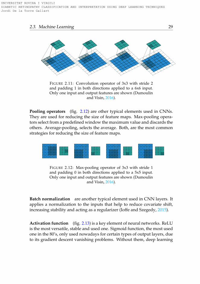
2.3. Machine Learning 29
FIGURE 2.11: Convolution operator of 3x3 with stride 2and padding 1 in both directions applied to a 6x6 input.Only one input and output features are shown (Dumoulin
and Visin, 2016).
Pooling operators (fig. 2.12) are other typical elements used in CNNs.They are used for reducing the size of feature maps. Max-pooling opera-tors select from a predefined window the maximum value and discards theothers. Average-pooling, selects the average. Both, are the most commonstrategies for reducing the size of feature maps.
2
2
3
0
3
0
0
1
0
3
0
0
2
1
2
0
2
2
3
1
1
2
3
1
0
3.0
3.0
3.0
2.0
3.0
3.0
3.0
3.0
3.0
2
2
3
0
3
0
0
1
0
3
0
0
2
1
2
0
2
2
3
1
1
2
3
1
0
3.0
3.0
3.0
2.0
3.0
3.0
3.0
3.0
3.0
2
2
3
0
3
0
0
1
0
3
0
0
2
1
2
0
2
2
3
1
1
2
3
1
0
3.0
3.0
3.0
2.0
3.0
3.0
3.0
3.0
3.0
2
2
3
0
3
0
0
1
0
3
0
0
2
1
2
0
2
2
3
1
1
2
3
1
0
3.0
3.0
3.0
2.0
3.0
3.0
3.0
3.0
3.0
FIGURE 2.12: Max-pooling operator of 3x3 with stride 1and padding 0 in both directions applied to a 5x5 input.Only one input and output features are shown (Dumoulin
and Visin, 2016).
Batch normalization are another typical element used in CNN layers. Itapplies a normalization to the inputs that help to reduce covariate shift,increasing stability and acting as a regularizer (Ioffe and Szegedy, 2015).
Activation function (fig. 2.13) is a key element of neural networks. ReLUis the most versatile, stable and used one. Sigmoid function, the most usedone in the 80’s, only used nowadays for certain types of output layers, dueto its gradient descent vanishing problems. Without them, deep learning
UNIVERSITAT ROVIRA I VIRGILI DIABETIC RETINOPATHY CLASSIFICATION AND INTERPRETATION USING DEEP LEARNING TECHNIQUES Jordi De la Torre Gallart
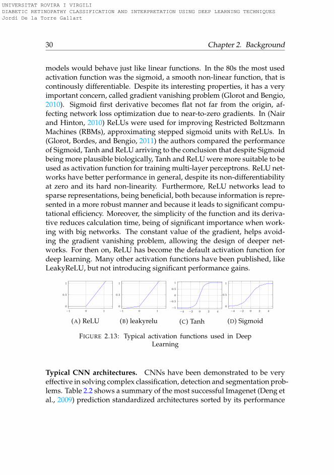
30 Chapter 2. Background
models would behave just like linear functions. In the 80s the most usedactivation function was the sigmoid, a smooth non-linear function, that iscontinously differentiable. Despite its interesting properties, it has a veryimportant concern, called gradient vanishing problem (Glorot and Bengio,2010). Sigmoid first derivative becomes flat not far from the origin, af-fecting network loss optimization due to near-to-zero gradients. In (Nairand Hinton, 2010) ReLUs were used for improving Restricted BoltzmannMachines (RBMs), approximating stepped sigmoid units with ReLUs. In(Glorot, Bordes, and Bengio, 2011) the authors compared the performanceof Sigmoid, Tanh and ReLU arriving to the conclusion that despite Sigmoidbeing more plausible biologically, Tanh and ReLU were more suitable to beused as activation function for training multi-layer perceptrons. ReLU net-works have better performance in general, despite its non-differentiabilityat zero and its hard non-linearity. Furthermore, ReLU networks lead tosparse representations, being beneficial, both because information is repre-sented in a more robust manner and because it leads to significant compu-tational efficiency. Moreover, the simplicity of the function and its deriva-tive reduces calculation time, being of significant importance when work-ing with big networks. The constant value of the gradient, helps avoid-ing the gradient vanishing problem, allowing the design of deeper net-works. For then on, ReLU has become the default activation function fordeep learning. Many other activation functions have been published, likeLeakyReLU, but not introducing significant performance gains.
−1 0 1
0
0.5
1
(A) ReLU
−1 0 1
0
0.5
1
(B) leakyrelu
−4 −2 0 2 4
−1
−0.5
0
0.5
1
(C) Tanh
−4 −2 0 2 4
0
0.5
1
(D) Sigmoid
FIGURE 2.13: Typical activation functions used in DeepLearning
Typical CNN architectures. CNNs have been demonstrated to be veryeffective in solving complex classification, detection and segmentation prob-lems. Table 2.2 shows a summary of the most successful Imagenet (Deng etal., 2009) prediction standardized architectures sorted by its performance
UNIVERSITAT ROVIRA I VIRGILI DIABETIC RETINOPATHY CLASSIFICATION AND INTERPRETATION USING DEEP LEARNING TECHNIQUES Jordi De la Torre Gallart
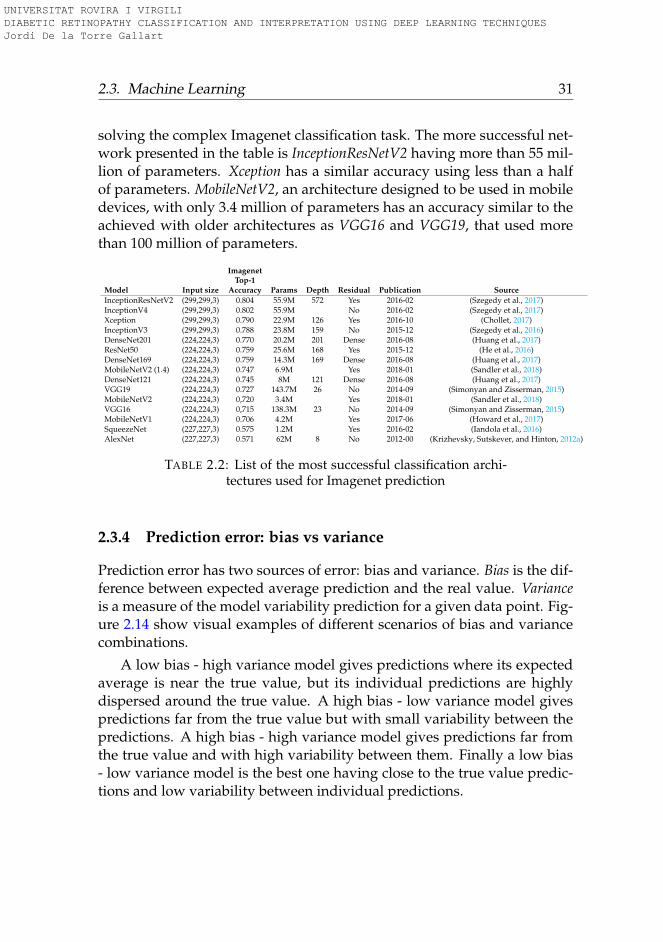
2.3. Machine Learning 31
solving the complex Imagenet classification task. The more successful net-work presented in the table is InceptionResNetV2 having more than 55 mil-lion of parameters. Xception has a similar accuracy using less than a halfof parameters. MobileNetV2, an architecture designed to be used in mobiledevices, with only 3.4 million of parameters has an accuracy similar to theachieved with older architectures as VGG16 and VGG19, that used morethan 100 million of parameters.
Model Input size
ImagenetTop-1
Accuracy Params Depth Residual Publication SourceInceptionResNetV2 (299,299,3) 0.804 55.9M 572 Yes 2016-02 (Szegedy et al., 2017)InceptionV4 (299,299,3) 0.802 55.9M No 2016-02 (Szegedy et al., 2017)Xception (299,299,3) 0.790 22.9M 126 Yes 2016-10 (Chollet, 2017)InceptionV3 (299,299,3) 0.788 23.8M 159 No 2015-12 (Szegedy et al., 2016)DenseNet201 (224,224,3) 0.770 20.2M 201 Dense 2016-08 (Huang et al., 2017)ResNet50 (224,224,3) 0.759 25.6M 168 Yes 2015-12 (He et al., 2016)DenseNet169 (224,224,3) 0.759 14.3M 169 Dense 2016-08 (Huang et al., 2017)MobileNetV2 (1.4) (224,224,3) 0.747 6.9M Yes 2018-01 (Sandler et al., 2018)DenseNet121 (224,224,3) 0.745 8M 121 Dense 2016-08 (Huang et al., 2017)VGG19 (224,224,3) 0.727 143.7M 26 No 2014-09 (Simonyan and Zisserman, 2015)MobileNetV2 (224,224,3) 0,720 3.4M Yes 2018-01 (Sandler et al., 2018)VGG16 (224,224,3) 0,715 138.3M 23 No 2014-09 (Simonyan and Zisserman, 2015)MobileNetV1 (224,224,3) 0.706 4.2M Yes 2017-06 (Howard et al., 2017)SqueezeNet (227,227,3) 0.575 1.2M Yes 2016-02 (Iandola et al., 2016)AlexNet (227,227,3) 0.571 62M 8 No 2012-00 (Krizhevsky, Sutskever, and Hinton, 2012a)
TABLE 2.2: List of the most successful classification archi-tectures used for Imagenet prediction
2.3.4 Prediction error: bias vs variance
Prediction error has two sources of error: bias and variance. Bias is the dif-ference between expected average prediction and the real value. Varianceis a measure of the model variability prediction for a given data point. Fig-ure 2.14 show visual examples of different scenarios of bias and variancecombinations.
A low bias - high variance model gives predictions where its expectedaverage is near the true value, but its individual predictions are highlydispersed around the true value. A high bias - low variance model givespredictions far from the true value but with small variability between thepredictions. A high bias - high variance model gives predictions far fromthe true value and with high variability between them. Finally a low bias- low variance model is the best one having close to the true value predic-tions and low variability between individual predictions.
UNIVERSITAT ROVIRA I VIRGILI DIABETIC RETINOPATHY CLASSIFICATION AND INTERPRETATION USING DEEP LEARNING TECHNIQUES Jordi De la Torre Gallart
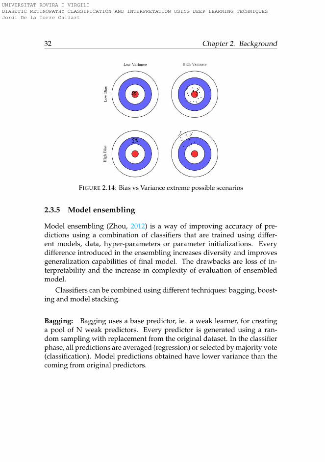
32 Chapter 2. Background
FIGURE 2.14: Bias vs Variance extreme possible scenarios
2.3.5 Model ensembling
Model ensembling (Zhou, 2012) is a way of improving accuracy of pre-dictions using a combination of classifiers that are trained using differ-ent models, data, hyper-parameters or parameter initializations. Everydifference introduced in the ensembling increases diversity and improvesgeneralization capabilities of final model. The drawbacks are loss of in-terpretability and the increase in complexity of evaluation of ensembledmodel.
Classifiers can be combined using different techniques: bagging, boost-ing and model stacking.
Bagging: Bagging uses a base predictor, ie. a weak learner, for creatinga pool of N weak predictors. Every predictor is generated using a ran-dom sampling with replacement from the original dataset. In the classifierphase, all predictions are averaged (regression) or selected by majority vote(classification). Model predictions obtained have lower variance than thecoming from original predictors.
UNIVERSITAT ROVIRA I VIRGILI DIABETIC RETINOPATHY CLASSIFICATION AND INTERPRETATION USING DEEP LEARNING TECHNIQUES Jordi De la Torre Gallart
2.4. Data 33
Boosting: Boosting predictor generation process is sequential, buildingmultiple incremental models to decrease bias, while keeping variance small.In every step, Boosting increases the weights of miss-classified data to em-phasize the importance of the most difficult cases. Boosting also assignsweights in the classification stage to predictors giving more importance tobest predictors. Due to this weighting strategy, boosting is able not onlyto reduce variance but also to reduce bias. In counterpart, boosting canover-fit training data, problem that is not present in bagging predictors.
Model stacking: allows the combination of model predictors of completelydifferent nature. It fits a meta-model such as for example, a logistic re-gression, using cross validation predictions coming from multiple models,achieving better results than source predictors.
2.4 Data
Data is at the core of any machine learning model, its quality determinesthe validity and generalization capabilities of any model derived from it.Machine learning paradigm is based, precisely, in the design of models thatare able to learn from data. In this section, we aim to make an exploratoryanalysis of the data sets that have been used for the elaboration of thisthesis.
2.4.1 Datasets
Three different datasets have been used: EyePACS, Messidor-2 and Reus.EyePACS, the biggest dataset available, have been used for model train-ing, validation and testing. Messidor-2 and Reus have been used for test-ing purposes and for checking validity of trained models over alternativepopulations.
UNIVERSITAT ROVIRA I VIRGILI DIABETIC RETINOPATHY CLASSIFICATION AND INTERPRETATION USING DEEP LEARNING TECHNIQUES Jordi De la Torre Gallart
34 Chapter 2. Background
2.4.2 EyePACS dataset
EyePACS dataset (EyePACS, 2018) is formed by the images of 44, 346 dif-ferent patients. For each one of them, left and right eye images are avail-able, having a total of 88, 692 retina fundus images. Each one of the imagesis classified according to the standards defined in (Wilkinson et al., 2003).The images are taken in variable conditions: by different cameras, in differ-ent illumination conditions and have different resolutions. The dataset ishighly imbalanced having 65, 343 class 0 images; 6, 195 of class 1; 13, 153 ofclass 2; 2, 087 of class 3 and 1, 914 of class 4. Figure 2.15a shows a graphicalrepresentation of the class distribution of the dataset.
2.4.3 Messidor-2 dataset
Messidor-2 dataset (Decencière et al., 2014) is formed by a total of 1, 748retina fundus images. Each one of the images has adjudicated grades forDiabetic Retinopathy Severity following (Wilkinson et al., 2003), DiabeticMacular Edema (DME) based on hard exudates classification, and Grad-ability. The grades were adjudicated by a panel of three Retina Specialists(Brain, 2018). This fact gives high confidence to the tagging (being nearBayes Optimal Error), making the dataset suitable to be used as a high con-fidence test set. The dataset is also highly imbalanced having 1, 017 class0 images; 270 of class 1; 347 of class 2; 75 of class 3 and 35 of class 4. Noexplicit differentiation between eyes of the same patient is given. Figure2.15b shows a graphical representation of its class distribution.
2.4.4 HUSJR dataset
We have been able to obtain a third dataset from a reference hospital inCatalonia region: Hospital Universitari Sant Joan de Reus (HUSJR). It islocated in Tarragona province, concretely in the city of Reus. The ophthal-mology unit of this hospital has collected data from population of Cau-casian, T2DM patients between January 1, 2007 and December 31, 2016.This included 85.33% of T2DM patients of this area. Patients have beenscreened with the nonmydriatic fundus camera units (NMCU) at HUSJR.Screening was carried out with one 45o field retinography, centered on thefovea. If DR was diagnosed, the patient was sent to the Ophthalmology
UNIVERSITAT ROVIRA I VIRGILI DIABETIC RETINOPATHY CLASSIFICATION AND INTERPRETATION USING DEEP LEARNING TECHNIQUES Jordi De la Torre Gallart
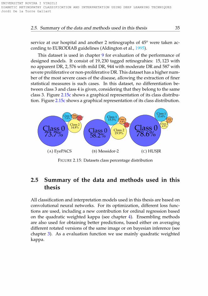
2.5. Summary of the data and methods used in this thesis 35
service at our hospital and another 2 retinographs of 45o were taken ac-cording to EURODIAB guidelines (Aldington et al., 1995).
This dataset is used in chapter 9 for evaluation of the performance ofdesigned models. It consist of 19, 230 tagged retinograhies: 15, 123 withno apparent DR, 2, 576 with mild DR, 944 with moderate DR and 587 withsevere proliferative or non-proliferative DR. This dataset has a higher num-ber of the most severe cases of the disease, allowing the extraction of finerstatistical measures is such cases. In this dataset, no differentiation be-tween class 3 and class 4 is given, considering that they belong to the sameclass 3. Figure 2.15c shows a graphical representation of its class distribu-tion. Figure 2.15c shows a graphical representation of its class distribution.
Class 073.7%
Class 17.0%
Class 214.8%
Class 32.3%Class 4
2.2%
(A) EyePACS
Class 058.2%
Class 115.5%
Class 219.9%
Class 34.4%
Class 42.0%
(B) Messidor-2
Class 078.6%
Class 113.4%
Class 24.9%
Class 33.1%
(C) HUSJR
FIGURE 2.15: Datasets class percentage distribution
2.5 Summary of the data and methods used in thisthesis
All classification and interpretation models used in this thesis are based onconvolutional neural networks. For its optimization, different loss func-tions are used, including a new contribution for ordinal regression basedon the quadratic weighted kappa (see chapter 4). Ensembling methodsare also used for obtaining better predictions, based either on averagingdifferent rotated versions of the same image or on bayesian inference (seechapter 3). As a evaluation function we use mainly quadratic weightedkappa.
UNIVERSITAT ROVIRA I VIRGILI DIABETIC RETINOPATHY CLASSIFICATION AND INTERPRETATION USING DEEP LEARNING TECHNIQUES Jordi De la Torre Gallart

36 Chapter 2. Background
Relating to data, all models are trained using different subsets of Eye-PACS dataset and tested using another subset of the same dataset. Messidor-2 is used for testing purposes in chapter 5 and for model fine-tuning of thelast classification layer in chapter 9. Reus dataset is used only for testingpurposes in chapter 9.
UNIVERSITAT ROVIRA I VIRGILI DIABETIC RETINOPATHY CLASSIFICATION AND INTERPRETATION USING DEEP LEARNING TECHNIQUES Jordi De la Torre Gallart

37
Part I
Classification
UNIVERSITAT ROVIRA I VIRGILI DIABETIC RETINOPATHY CLASSIFICATION AND INTERPRETATION USING DEEP LEARNING TECHNIQUES Jordi De la Torre Gallart

UNIVERSITAT ROVIRA I VIRGILI DIABETIC RETINOPATHY CLASSIFICATION AND INTERPRETATION USING DEEP LEARNING TECHNIQUES Jordi De la Torre Gallart
39
Chapter 3
Preliminary Models
In this chapter we present the models that where designed in the earlystage of the thesis. The aim of this work was to understand better theproblem, ie. explore different input sizes, types of models, data augmenta-tion techniques and hyper-parameters and explore the possibilities of us-ing deep learning for successfully solving this task. They where publishedin (Torre, Valls, and Puig, 2016a).
3.1 Introduction
In the last decade, several attempts to automatize the DR diagnosis throughimages of the eye fundus have been tested. They are basically focused onapplying well-known pattern recognition models. In this work, we wantto apply a Deep Convolutional Neural Network (DCNN) model, as it hasbeen proven to be a very effective algorithm to solve general image clas-sification problems. DCNN is a supervised learning model for automaticclassification that does not require any pretreatment of the images, nor anyfeature analysis.
Deep learning techniques are focused on learning multiple levels ofrepresentation and abstraction that help to make sense of the hidden in-formation in data such as images. In this way having a complete set ofcorrectly classified images and without having any a priori understand-ing of the features required to make the classification, the system is able tolearn the properties of the image that minimize a defined cost function thatis direct or indirectly related with the classification score index that has to
UNIVERSITAT ROVIRA I VIRGILI DIABETIC RETINOPATHY CLASSIFICATION AND INTERPRETATION USING DEEP LEARNING TECHNIQUES Jordi De la Torre Gallart
40 Chapter 3. Preliminary Models
be optimized. In this chapter we show that a DCNN is able to learn fromdata the most important features to make the classification of retinal im-ages into the five DR categories, without the need of a hand-crafted featureextraction process.
In this chapter we explore methods for classifying retina images intothe five different classes of DR defined in chapter 2, that are:
0. - No apparent retinopathy
1. - Mild Non-Proliferative Diabetic Retinopathy (NPDR)
2. - Moderate NPDR
3. - Severe NPDR
4. - Proliferative DR
The chapter is organized as follows: we present the related work, nextwe explain the characteristics of the available data and why deep learningtechniques can be applied over them, next we explain the methodologyused for solving the problem, we show the obtained results and finally weexpose the conclusions and further steps for improving the results.
3.2 Related work
Traditional models of pattern recognition in images since the late 50s havebeen based on extracting hand-crafted fixed engineered features or fixedkernels from the image and, then, using a trainable classifier on top ofthose features to get the final classification. Using this model, the prob-lem of the DR detection has been tackled by feature extraction using onhand models targeted to the detection of microaneurisms, haemorrhagesand exudates in retinal images (e.g. (Sudha and Thirupurasundari, 2014),(Torrents-Barrena et al., 2015), etc).
This type of approach requires a good understanding of disease mech-anisms to be able to find the important features present in the image. Thisknowledge is specific of the problem to be solved, requires a lot of labor
UNIVERSITAT ROVIRA I VIRGILI DIABETIC RETINOPATHY CLASSIFICATION AND INTERPRETATION USING DEEP LEARNING TECHNIQUES Jordi De la Torre Gallart
3.3. Data 41
time and is task specific and thereby not reusable for other different classi-fication problems.
Deep learning is a new powerful method for supervised learning. Byadding more layers and more units within a layer of a neural network, wecan represent functions of increasing complexity. Training must be doneon sufficiently large annotated image data sets. In computer vision classi-fication problems, neural networks have largely displaced the traditionalapproaches based on handcrafted features. They have proved to be thebest available method for solving the biggest classification challenges, likefor example IMAGENET (Russakovsky et al., 2015). In this previous typeof image analysis problems, distinct objects should be recognized on dif-ferent types of images. In the case of DR classification, all images are verysimilar (as they are retina photos) and very small and vague lesions haveto be detected at different locations in order to find the correct severity cat-egory of DR. This chapter, thus, wants to study the performance of DCNNsfor this kind of medical image analysis.
3.3 Data
We use the EyePACS dataset presented in chapter 2. We split the datasetusing random selection in two disjoint sets. The training set contains 35,126images; 25,810 of class 0, 2,443 of class 1, 5,292 of class 2, 873 of class 3 and708 of class 4. The test set contains a total of 53,576 images; 39,533 of class0, 3,762 of class 1, 7,861 of class 2, 1,214 of class 3 and 1,206 of class 4.
3.4 Methodology for retinal image classification
All the state-of-the-art architectures for supervised deep learning over im-ages (e.g. AlexNet (Krizhevsky, Sutskever, and Hinton, 2012b), GoogleNet(Szegedy et al., 2015) and VGGNet (Simonyan and Zisserman, 2015)) arebased on convolutional neural networks (CNNs). A set of convolutionallayers with dimensional down-sizing blocks between them, also knownas pooling layers, extract the statistical information from the data (featureextraction) that is passed to the posterior layers to construct more elabo-rate abstractions (features of features) that are useful for the classification.
UNIVERSITAT ROVIRA I VIRGILI DIABETIC RETINOPATHY CLASSIFICATION AND INTERPRETATION USING DEEP LEARNING TECHNIQUES Jordi De la Torre Gallart
42 Chapter 3. Preliminary Models
As a final stage a fully connected set of layers perform the classificationbased on the information coming from the last layers of the convolutionalnetwork. This kind of structure provides an end to end learning process,where either the classes or the features are learned from data with no hu-man intervention.
Next we explain the different phases of the DCNN construction for per-forming DR detection based on the available data: evaluation function,data pre-processing and data augmentation, model, training, testing andprobabilistic combination of the models of both eyes.
3.4.1 Evaluation function
The performance of the classification model is measured using the quadraticweighted kappa (QWK) index (see eq. 3.1), defined previously in chapter 2.As a brief summary, QWK, also known as Cohen’s Kappa, measures inter-rater agreement for categorical items in multi-class classification problems(Fleiss, Cohen, and Everitt, 1969), penalizing the discrepancy quadrati-cally with the distance from the correct class. It is generally thought to bea more robust measure than simple percent agreement calculation, sinceQWK takes into account the agreement occurring by chance. This met-ric typically varies from 0 (random agreement) to 1 (complete agreement).Negative values are also possible, the maximum possible negative value(-1) indicates a complete disagreement between classes. Being Oi,j the ob-served values, Ei,j the expected ones and C number of classes, QWK isdefined as:
κ = 1− ∑Ci=1 ∑C
j=1 ωi,jOi,j
∑Ci=1 ∑C
j=1 ωi,jEi,jwhere ωi,j =
(i− j)2
(C− 1)2 (3.1)
The QWK coefficient is used to compare the performance of differentprediction models and with the performance of the human experts (SE etal., 1985). Individual human experts report values of QWK of about 0.80in the prediction of the correct class in the DR disease. This value is con-sidered excellent because small discrepancies between the class predictiondoes not affect the treatment of the disease. The most important is the dif-ferentiation between presence or absence of the disease.
UNIVERSITAT ROVIRA I VIRGILI DIABETIC RETINOPATHY CLASSIFICATION AND INTERPRETATION USING DEEP LEARNING TECHNIQUES Jordi De la Torre Gallart
3.4. Methodology for retinal image classification 43
3.4.2 Data pre-processing and data augmentation
Firstly, DCNNs require large data-sets in order to avoid overfitting. A classbalanced data-set is also desirable as well (MA et al., 2008). One of theproven approaches that has good results to get more data from small data-sets is to use data augmentation techniques (Krizhevsky, Sutskever, andHinton, 2012b). The data augmentation is done in two stages: first a copyof the training examples of the small classes is done until they have thesame number of images as the biggest class. This generates an equilibratedtraining set. After this first step, to every image the next transformationsare applied in order to diversify the training examples:
• Cropping, random uniform
• Rotation (0◦ to 360◦), random uniform
• Mirroring ( X and Y axes), random uniform
• Brightness correction, random gaussian (σ = 0.1)
• Contrast correction, random gaussian (σ = 0.1)
All these transformations are applied to every image of the balancedtraining set and redone for every training epoch. This transformations as-sure that every image of the training set is different between each other forevery epoch, making the final prediction invariant to rotation, brightnessand contrast over the training set.
Secondly, DCNNs perform better when then input data is normalizedby having mean equal to 0 and standard deviation equal to 1, on each chan-nel (RGB). Thus, a normalization must be done on each image.
3.4.3 Model
The well-known LeCun et al. architecture has been taken (LeCun et al.,1998). It is composed by a series of convolutional layers followed by activa-tion function blocks, with some max-pooling dimensional reducing blocks.At the end, a final fully connected layer performs the classification and, fi-nally, a softmax output layer gives a probability estimation of every class(Figure 3.1).
UNIVERSITAT ROVIRA I VIRGILI DIABETIC RETINOPATHY CLASSIFICATION AND INTERPRETATION USING DEEP LEARNING TECHNIQUES Jordi De la Torre Gallart
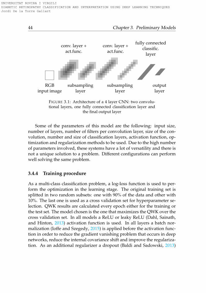
44 Chapter 3. Preliminary Models
RGBinput image
conv. layer +act.func.
subsamplinglayer
conv. layer +act.func.
subsamplinglayer
fully connectedclassific.
layer
outputlayer
FIGURE 3.1: Architecture of a 4 layer CNN: two convolu-tional layers, one fully connected classification layer and
the final output layer
Some of the parameters of this model are the following: input size,number of layers, number of filters per convolution layer, size of the con-volution, number and size of classification layers, activation function, op-timization and regularization methods to be used. Due to the high numberof parameters involved, these systems have a lot of versatility and there isnot a unique solution to a problem. Different configurations can performwell solving the same problem.
3.4.4 Training procedure
As a multi-class classification problem, a log-loss function is used to per-form the optimization in the learning stage. The original training set issplitted in two random subsets: one with 90% of the data and other with10%. The last one is used as a cross validation set for hyperparameter se-lection. QWK results are calculated every epoch either for the training orthe test set. The model chosen is the one that maximizes the QWK over thecross validation set. In all models a ReLU or leaky ReLU (Dahl, Sainath,and Hinton, 2013) activation function is used. In all layers a batch nor-malization (Ioffe and Szegedy, 2015) is applied before the activation func-tion in order to reduce the gradient vanishing problem that occurs in deepnetworks, reduce the internal covariance shift and improve the regulariza-tion. As an additional regularizer a dropout (Baldi and Sadowski, 2013)
UNIVERSITAT ROVIRA I VIRGILI DIABETIC RETINOPATHY CLASSIFICATION AND INTERPRETATION USING DEEP LEARNING TECHNIQUES Jordi De la Torre Gallart
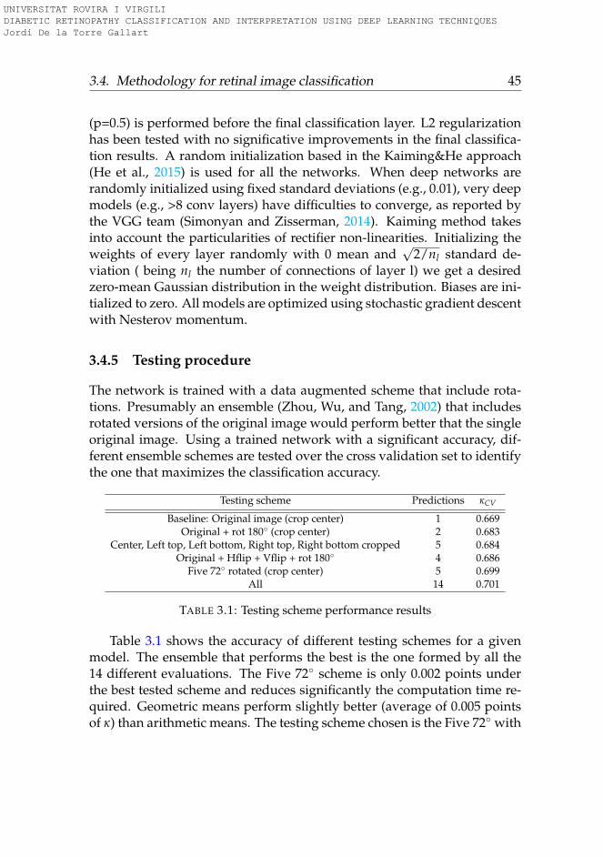
3.4. Methodology for retinal image classification 45
(p=0.5) is performed before the final classification layer. L2 regularizationhas been tested with no significative improvements in the final classifica-tion results. A random initialization based in the Kaiming&He approach(He et al., 2015) is used for all the networks. When deep networks arerandomly initialized using fixed standard deviations (e.g., 0.01), very deepmodels (e.g., >8 conv layers) have difficulties to converge, as reported bythe VGG team (Simonyan and Zisserman, 2014). Kaiming method takesinto account the particularities of rectifier non-linearities. Initializing theweights of every layer randomly with 0 mean and
√2/nl standard de-
viation ( being nl the number of connections of layer l) we get a desiredzero-mean Gaussian distribution in the weight distribution. Biases are ini-tialized to zero. All models are optimized using stochastic gradient descentwith Nesterov momentum.
3.4.5 Testing procedure
The network is trained with a data augmented scheme that include rota-tions. Presumably an ensemble (Zhou, Wu, and Tang, 2002) that includesrotated versions of the original image would perform better that the singleoriginal image. Using a trained network with a significant accuracy, dif-ferent ensemble schemes are tested over the cross validation set to identifythe one that maximizes the classification accuracy.
Testing scheme Predictions κCV
Baseline: Original image (crop center) 1 0.669Original + rot 180◦ (crop center) 2 0.683
Center, Left top, Left bottom, Right top, Right bottom cropped 5 0.684Original + Hflip + Vflip + rot 180◦ 4 0.686
Five 72◦ rotated (crop center) 5 0.699All 14 0.701
TABLE 3.1: Testing scheme performance results
Table 3.1 shows the accuracy of different testing schemes for a givenmodel. The ensemble that performs the best is the one formed by all the14 different evaluations. The Five 72◦ scheme is only 0.002 points underthe best tested scheme and reduces significantly the computation time re-quired. Geometric means perform slightly better (average of 0.005 pointsof κ) than arithmetic means. The testing scheme chosen is the Five 72◦ with
UNIVERSITAT ROVIRA I VIRGILI DIABETIC RETINOPATHY CLASSIFICATION AND INTERPRETATION USING DEEP LEARNING TECHNIQUES Jordi De la Torre Gallart
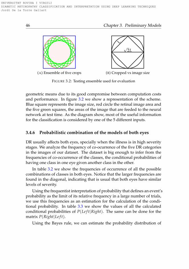
46 Chapter 3. Preliminary Models
(A) Ensemble of five crops
√2L
L
(B) Cropped vs image size
FIGURE 3.2: Testing ensemble used for evaluation
geometric means due to its good compromise between computation costsand performance. In figure 3.2 we show a representation of the scheme.Blue square represents the image size, red circle the retinal image area andthe five green squares, the areas of the image that are feeded to the neuralnetwork at test time. As the diagram show, most of the useful informationfor the classification is considered by one of the 5 different inputs.
3.4.6 Probabilistic combination of the models of both eyes
DR usually affects both eyes, specially when the illness is in high severitystages. We analyze the frequency of co-ocurrence of the five DR categoriesin the images of our dataset. The dataset is big enough to infer from thefrequencies of co-occurrence of the classes, the conditional probabilities ofhaving one class in one eye given another class in the other.
In table 3.2 we show the frequencies of occurrence of all the possiblecombinations of classes in both eyes. Notice that the larger frequencies arefound in the diagonal, indicating that is usual that both eyes have similarlevels of severity.
Using the frequentist interpretation of probability that defines an event’sprobability as the limit of its relative frequency in a large number of trials,we use this frequencies as an estimation for the calculation of the condi-tional probability. In table 3.3 we show the values of all the calculatedconditional probabilities of P(Le f t|Right). The same can be done for thematrix P(Right|Le f t).
Using the Bayes rule, we can estimate the probability distribution of
UNIVERSITAT ROVIRA I VIRGILI DIABETIC RETINOPATHY CLASSIFICATION AND INTERPRETATION USING DEEP LEARNING TECHNIQUES Jordi De la Torre Gallart
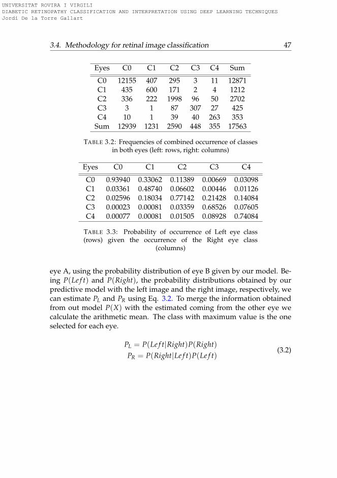
3.4. Methodology for retinal image classification 47
Eyes C0 C1 C2 C3 C4 Sum
C0 12155 407 295 3 11 12871C1 435 600 171 2 4 1212C2 336 222 1998 96 50 2702C3 3 1 87 307 27 425C4 10 1 39 40 263 353
Sum 12939 1231 2590 448 355 17563
TABLE 3.2: Frequencies of combined occurrence of classesin both eyes (left: rows, right: columns)
Eyes C0 C1 C2 C3 C4
C0 0.93940 0.33062 0.11389 0.00669 0.03098C1 0.03361 0.48740 0.06602 0.00446 0.01126C2 0.02596 0.18034 0.77142 0.21428 0.14084C3 0.00023 0.00081 0.03359 0.68526 0.07605C4 0.00077 0.00081 0.01505 0.08928 0.74084
TABLE 3.3: Probability of occurrence of Left eye class(rows) given the occurrence of the Right eye class
(columns)
eye A, using the probability distribution of eye B given by our model. Be-ing P(Le f t) and P(Right), the probability distributions obtained by ourpredictive model with the left image and the right image, respectively, wecan estimate PL and PR using Eq. 3.2. To merge the information obtainedfrom out model P(X) with the estimated coming from the other eye wecalculate the arithmetic mean. The class with maximum value is the oneselected for each eye.
PL = P(Le f t|Right)P(Right)PR = P(Right|Le f t)P(Le f t)
(3.2)
UNIVERSITAT ROVIRA I VIRGILI DIABETIC RETINOPATHY CLASSIFICATION AND INTERPRETATION USING DEEP LEARNING TECHNIQUES Jordi De la Torre Gallart
48 Chapter 3. Preliminary Models
3.5 Experiments
Different experiments have been conducted to analyze the quality of theclassification with different parameters of the DCNN. First, we perform anstudy of the best image size. Due to the type of image classification thatis done, it is crucial to choose the right size of the input images in orderto detect the important features involved in the RD severity detection. Asexplained before, cropping is part of the data augmentation scheme. Theoriginal size is chosen from the NN input size as
√2 times the input size.
In this way, due to the circular nature of the retina, we maximize the usefulinformation of the square cropped from the center of the image (see Fig.3.2). The input sizes tested are:
• Resizing to 181x181 cropped to 128x128 NN input
• Resizing to 362x362 cropped to 256x256 NN input
• Resizing to 543x543 cropped to 384x384 NN input
• Resizing to 724x724 cropped to 512x512 NN input
Different number of layers have also been studied for each image size.In table 3.4 are presented the higher classification rates obtained from thebest models obtained for different input sizes. The number of layers of thebest models are also shown.
Layers Input size κtest FN FP
12 (3,128,128) 0.488 11.6% 11.5%14 (3,256,256) 0.636 4.4% 28.7%16 (3,384,384) 0.668 7.9% 14.9%16 (3,512,512) 0.725 5.0% 11.9%
TABLE 3.4: Best classification results for different inputsizes
As the input size and the complexity of the network is increased theresults obtained become better. Greater sizes give more definition of the
UNIVERSITAT ROVIRA I VIRGILI DIABETIC RETINOPATHY CLASSIFICATION AND INTERPRETATION USING DEEP LEARNING TECHNIQUES Jordi De la Torre Gallart
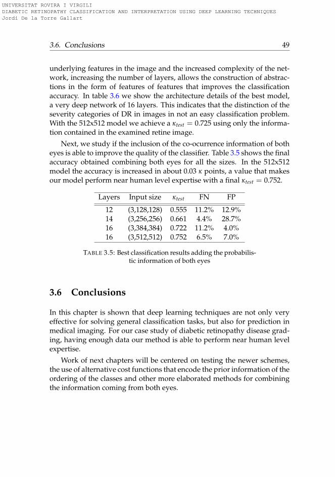
3.6. Conclusions 49
underlying features in the image and the increased complexity of the net-work, increasing the number of layers, allows the construction of abstrac-tions in the form of features of features that improves the classificationaccuracy. In table 3.6 we show the architecture details of the best model,a very deep network of 16 layers. This indicates that the distinction of theseverity categories of DR in images in not an easy classification problem.With the 512x512 model we achieve a κtest = 0.725 using only the informa-tion contained in the examined retine image.
Next, we study if the inclusion of the co-ocurrence information of botheyes is able to improve the quality of the classifier. Table 3.5 shows the finalaccuracy obtained combining both eyes for all the sizes. In the 512x512model the accuracy is increased in about 0.03 κ points, a value that makesour model perform near human level expertise with a final κtest = 0.752.
Layers Input size κtest FN FP
12 (3,128,128) 0.555 11.2% 12.9%14 (3,256,256) 0.661 4.4% 28.7%16 (3,384,384) 0.722 11.2% 4.0%16 (3,512,512) 0.752 6.5% 7.0%
TABLE 3.5: Best classification results adding the probabilis-tic information of both eyes
3.6 Conclusions
In this chapter is shown that deep learning techniques are not only veryeffective for solving general classification tasks, but also for prediction inmedical imaging. For our case study of diabetic retinopathy disease grad-ing, having enough data our method is able to perform near human levelexpertise.
Work of next chapters will be centered on testing the newer schemes,the use of alternative cost functions that encode the prior information of theordering of the classes and other more elaborated methods for combiningthe information coming from both eyes.
UNIVERSITAT ROVIRA I VIRGILI DIABETIC RETINOPATHY CLASSIFICATION AND INTERPRETATION USING DEEP LEARNING TECHNIQUES Jordi De la Torre Gallart
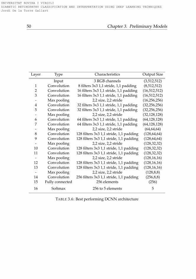
50 Chapter 3. Preliminary Models
Layer Type Characteristics Output Size
Input 3 RGB channels (3,512,512)1 Convolution 8 filters 3x3 1,1 stride, 1,1 padding (8,512,512)2 Convolution 16 filters 3x3 1,1 stride, 1,1 padding (16,512,512)3 Convolution 16 filters 3x3 1,1 stride, 1,1 padding (16,512,512)- Max pooling 2,2 size, 2,2 stride (16,256,256)4 Convolution 32 filters 3x3 1,1 stride, 1,1 padding (32,256,256)5 Convolution 32 filters 3x3 1,1 stride, 1,1 padding (32,256,256)- Max pooling 2,2 size, 2,2 stride (32,128,128)6 Convolution 64 filters 3x3 1,1 stride, 1,1 padding (64,128,128)7 Convolution 64 filters 3x3 1,1 stride, 1,1 padding (64,128,128)- Max pooling 2,2 size, 2,2 stride (64,64,64)8 Convolution 128 filters 3x3 1,1 stride, 1,1 padding (128,64,64)9 Convolution 128 filters 3x3 1,1 stride, 1,1 padding (128,64,64)- Max pooling 2,2 size, 2,2 stride (128,32,32)
10 Convolution 128 filters 3x3 1,1 stride, 1,1 padding (128,32,32)11 Convolution 128 filters 3x3 1,1 stride, 1,1 padding (128,32,32)- Max pooling 2,2 size, 2,2 stride (128,16,16)
12 Convolution 128 filters 3x3 1,1 stride, 1,1 padding (128,16,16)13 Convolution 128 filters 3x3 1,1 stride, 1,1 padding (128,16,16)- Max pooling 2,2 size, 2,2 stride (128,8,8)
14 Convolution 256 filters 3x3 1,1 stride, 1,1 padding (256,8,8)15 Fully connected 256 elements (256)
16 Softmax 256 to 5 elements 5
TABLE 3.6: Best performing DCNN architecture
UNIVERSITAT ROVIRA I VIRGILI DIABETIC RETINOPATHY CLASSIFICATION AND INTERPRETATION USING DEEP LEARNING TECHNIQUES Jordi De la Torre Gallart
51
Chapter 4
Kappa a Loss Function forOrdinal Regression
The aim of this work was to study the possibilities of using the QuadraticWeighted Kappa evaluation function as a loss function for optimizing deepneural networks. In this chapter we explore the usage of QWK for ordinalregression using deep learning models. For this purpose 3 case studiesof completely different nature are presented, proving an increase of morethan 5% in results over traditional log-loss optimization. This method gen-eralize directly to other multi-class classification problems where there is aprior known information about the predefined ordering of the classes. Thework presented in this chapter have been published in the paper (Torre,Puig, and Valls, 2018).
4.1 Introduction
Optimization of neural networks for multi-class classification is tradition-ally done using logarithmic loss. Logarithmic loss has a very robust prob-abilistic foundation: minimizing it, is the same as minimizing the loga-rithmic likelihood, that is equivalent to do a Maximum Likelihood Estima-tion (MLE) or equivalently, to find the Maximum a Posteriori Probability(MAP), given a uniform prior (Murphy, 2012). This loss function is de-signed to find perpendicular vectors in the output space. This model issuitable when output classes are independent, but it may not be good in
UNIVERSITAT ROVIRA I VIRGILI DIABETIC RETINOPATHY CLASSIFICATION AND INTERPRETATION USING DEEP LEARNING TECHNIQUES Jordi De la Torre Gallart
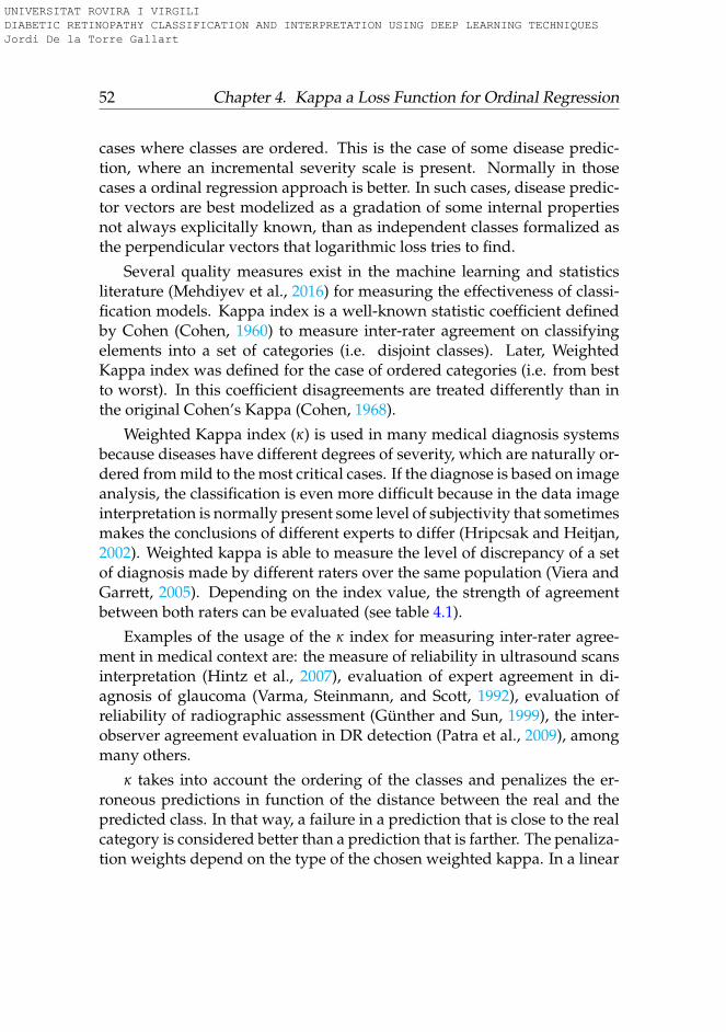
52 Chapter 4. Kappa a Loss Function for Ordinal Regression
cases where classes are ordered. This is the case of some disease predic-tion, where an incremental severity scale is present. Normally in thosecases a ordinal regression approach is better. In such cases, disease predic-tor vectors are best modelized as a gradation of some internal propertiesnot always explicitally known, than as independent classes formalized asthe perpendicular vectors that logarithmic loss tries to find.
Several quality measures exist in the machine learning and statisticsliterature (Mehdiyev et al., 2016) for measuring the effectiveness of classi-fication models. Kappa index is a well-known statistic coefficient definedby Cohen (Cohen, 1960) to measure inter-rater agreement on classifyingelements into a set of categories (i.e. disjoint classes). Later, WeightedKappa index was defined for the case of ordered categories (i.e. from bestto worst). In this coefficient disagreements are treated differently than inthe original Cohen’s Kappa (Cohen, 1968).
Weighted Kappa index (κ) is used in many medical diagnosis systemsbecause diseases have different degrees of severity, which are naturally or-dered from mild to the most critical cases. If the diagnose is based on imageanalysis, the classification is even more difficult because in the data imageinterpretation is normally present some level of subjectivity that sometimesmakes the conclusions of different experts to differ (Hripcsak and Heitjan,2002). Weighted kappa is able to measure the level of discrepancy of a setof diagnosis made by different raters over the same population (Viera andGarrett, 2005). Depending on the index value, the strength of agreementbetween both raters can be evaluated (see table 4.1).
Examples of the usage of the κ index for measuring inter-rater agree-ment in medical context are: the measure of reliability in ultrasound scansinterpretation (Hintz et al., 2007), evaluation of expert agreement in di-agnosis of glaucoma (Varma, Steinmann, and Scott, 1992), evaluation ofreliability of radiographic assessment (Günther and Sun, 1999), the inter-observer agreement evaluation in DR detection (Patra et al., 2009), amongmany others.
κ takes into account the ordering of the classes and penalizes the er-roneous predictions in function of the distance between the real and thepredicted class. In that way, a failure in a prediction that is close to the realcategory is considered better than a prediction that is farther. The penaliza-tion weights depend on the type of the chosen weighted kappa. In a linear
UNIVERSITAT ROVIRA I VIRGILI DIABETIC RETINOPATHY CLASSIFICATION AND INTERPRETATION USING DEEP LEARNING TECHNIQUES Jordi De la Torre Gallart
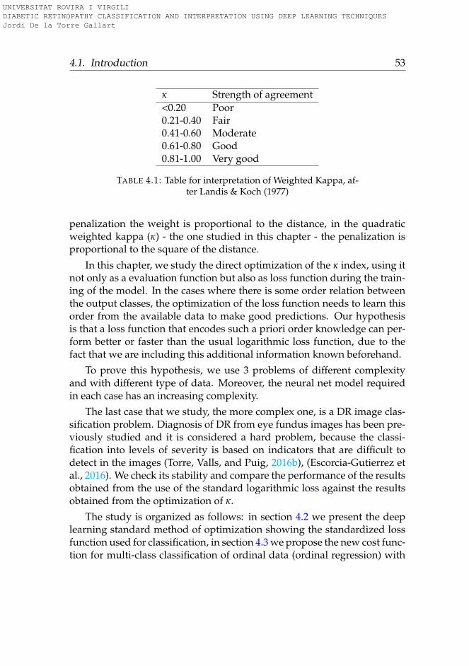
4.1. Introduction 53
κ Strength of agreement<0.20 Poor0.21-0.40 Fair0.41-0.60 Moderate0.61-0.80 Good0.81-1.00 Very good
TABLE 4.1: Table for interpretation of Weighted Kappa, af-ter Landis & Koch (1977)
penalization the weight is proportional to the distance, in the quadraticweighted kappa (κ) - the one studied in this chapter - the penalization isproportional to the square of the distance.
In this chapter, we study the direct optimization of the κ index, using itnot only as a evaluation function but also as loss function during the train-ing of the model. In the cases where there is some order relation betweenthe output classes, the optimization of the loss function needs to learn thisorder from the available data to make good predictions. Our hypothesisis that a loss function that encodes such a priori order knowledge can per-form better or faster than the usual logarithmic loss function, due to thefact that we are including this additional information known beforehand.
To prove this hypothesis, we use 3 problems of different complexityand with different type of data. Moreover, the neural net model requiredin each case has an increasing complexity.
The last case that we study, the more complex one, is a DR image clas-sification problem. Diagnosis of DR from eye fundus images has been pre-viously studied and it is considered a hard problem, because the classi-fication into levels of severity is based on indicators that are difficult todetect in the images (Torre, Valls, and Puig, 2016b), (Escorcia-Gutierrez etal., 2016). We check its stability and compare the performance of the resultsobtained from the use of the standard logarithmic loss against the resultsobtained from the optimization of κ.
The study is organized as follows: in section 4.2 we present the deeplearning standard method of optimization showing the standardized lossfunction used for classification, in section 4.3 we propose the new cost func-tion for multi-class classification of ordinal data (ordinal regression) with
UNIVERSITAT ROVIRA I VIRGILI DIABETIC RETINOPATHY CLASSIFICATION AND INTERPRETATION USING DEEP LEARNING TECHNIQUES Jordi De la Torre Gallart
54 Chapter 4. Kappa a Loss Function for Ordinal Regression
all the mathematical equations required for the optimization using first or-der gradient descent algorithms, in section 4.4 we define the experiments,in section 4.5 we present the results obtained and finally in section 4.6 wepresent the conclusions of the chapter.
4.2 Deep learning method
Supervised deep learning techniques are recently used extensively for manyautomatic classification tasks. In the case of images, most of the state of theart methods are based on the use of deep convolutional neural networks(DCNN): CIFAR-10 (Graham, 2014), CIFAR-100 (Clevert, Unterthiner, andHochreiter, 2015), STL10 (Dundar, Jin, and Culurciello, 2015), SVHN (Liaoand Carneiro, 2015), ImageNet (Krizhevsky, Sutskever, and Hinton, 2012a),among many others. These techniques are focused on learning multiplelevels of representation and abstraction that help to make sense of the hid-den information in data such as images. In this way, having a completeset of correctly classified images and without any a priori understandingof the features, the model is able to learn the properties of the image thatminimize a defined cost function that is direct or indirectly related with theclassification score index to optimize.
ImageInput
FeatureExtrac-
tionLayers
Classi-ficationLayers
ClassProb-ability
CostFunction
FIGURE 4.1: High level description of a deep learning im-age classification scheme
As shown in Fig. 4.1 for image classification, several convolutional neu-ral networks are optimized for making a good feature extraction. Theselayers are followed by one or more classification layers. Finally, the lastoutput layer is formed by as many outputs as classes to predict. In the out-put layer is usual to have a soft-max function that represents the outputprobability of every class to predict. Normally, the class assigned to theimage is the one with the highest value of probability.
The main parameters to define are: total number of layers, the size ofthe convolutions with its stride and padding, the activation function to use,
UNIVERSITAT ROVIRA I VIRGILI DIABETIC RETINOPATHY CLASSIFICATION AND INTERPRETATION USING DEEP LEARNING TECHNIQUES Jordi De la Torre Gallart
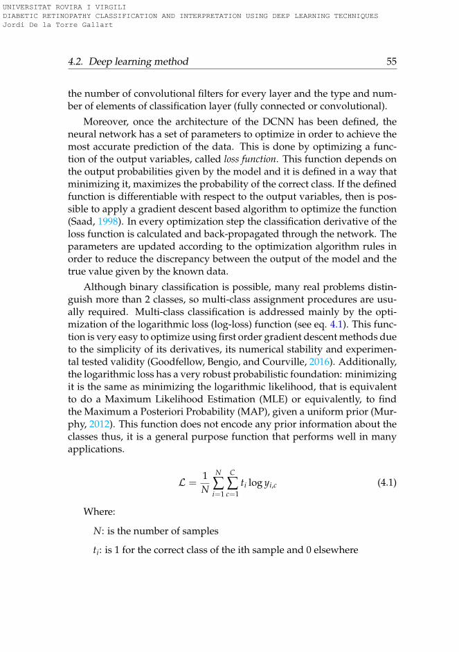
4.2. Deep learning method 55
the number of convolutional filters for every layer and the type and num-ber of elements of classification layer (fully connected or convolutional).
Moreover, once the architecture of the DCNN has been defined, theneural network has a set of parameters to optimize in order to achieve themost accurate prediction of the data. This is done by optimizing a func-tion of the output variables, called loss function. This function depends onthe output probabilities given by the model and it is defined in a way thatminimizing it, maximizes the probability of the correct class. If the definedfunction is differentiable with respect to the output variables, then is pos-sible to apply a gradient descent based algorithm to optimize the function(Saad, 1998). In every optimization step the classification derivative of theloss function is calculated and back-propagated through the network. Theparameters are updated according to the optimization algorithm rules inorder to reduce the discrepancy between the output of the model and thetrue value given by the known data.
Although binary classification is possible, many real problems distin-guish more than 2 classes, so multi-class assignment procedures are usu-ally required. Multi-class classification is addressed mainly by the opti-mization of the logarithmic loss (log-loss) function (see eq. 4.1). This func-tion is very easy to optimize using first order gradient descent methods dueto the simplicity of its derivatives, its numerical stability and experimen-tal tested validity (Goodfellow, Bengio, and Courville, 2016). Additionally,the logarithmic loss has a very robust probabilistic foundation: minimizingit is the same as minimizing the logarithmic likelihood, that is equivalentto do a Maximum Likelihood Estimation (MLE) or equivalently, to findthe Maximum a Posteriori Probability (MAP), given a uniform prior (Mur-phy, 2012). This function does not encode any prior information about theclasses thus, it is a general purpose function that performs well in manyapplications.
L =1N
N
∑i=1
C
∑c=1
ti log yi,c (4.1)
Where:
N: is the number of samples
ti: is 1 for the correct class of the ith sample and 0 elsewhere
UNIVERSITAT ROVIRA I VIRGILI DIABETIC RETINOPATHY CLASSIFICATION AND INTERPRETATION USING DEEP LEARNING TECHNIQUES Jordi De la Torre Gallart
56 Chapter 4. Kappa a Loss Function for Ordinal Regression
C: is the number of classes
On the other hand, there are applications where we have a priori in-formation about some properties of the classes to predict. For example,in the case of ordinal regression, the different categories are sorted in apredefined way, representing a gradation of the output classes. When thelog-loss is applied for the classification in this type of problems, the modelhas to learn such ordering from the data in order to obtain enough accu-racy of the classification rate. In this case, a specialized loss like weightedkappa could be more appropriate than a general loss like the logarithm. Inthe rest of this chapter we will study if Weighted Kappa can perform betteror even faster, due to the fact that it does not need to learn the order fromthe available data.
4.3 Weighted kappa as loss function in deep learning
In this section we present our contribution to the optimization of neuralnetworks in general and deep learning in particular using Weighted Kappaindex. Weighted Kappa has been normally used as an index to measure theinter-rating agreement between raters in a multi-class classification prob-lem where the categories have an a priori defined ordering, in such a waythat the classes to categorize are a high level abstraction of some sort ofintrinsic information that we want to extract from data.
Three matrices are involved in the calculation of this index: the matrixof observed scores, O, the matrix of expected scores based on chance agree-ment, E, and the weight matrix, ω. The Weighted Kappa is defined as eq.4.2.
κ = 1− ∑i,j ωi,jOi,j
∑i,j ωi,jEi,j(4.2)
, where:
C: is the number of classes
i, j ∈ {1, 2, ..., C}
UNIVERSITAT ROVIRA I VIRGILI DIABETIC RETINOPATHY CLASSIFICATION AND INTERPRETATION USING DEEP LEARNING TECHNIQUES Jordi De la Torre Gallart
4.3. Weighted kappa as loss function in deep learning 57
Oi,j: the number of observations classified in the i-th category by theprediction model and they are in the j-th category in the correct clas-sification (i.e. "true value").
Ei,j: outer product between the two classification histogram vectors(prediction and "true value"), normalized such that E and O have thesame sum.
ωi,j: weight penalization for every pair i, j. Generally, ωi,j =(i−j)n
(C−1)n .For linear penalization n = 1. For quadratic penalization (more com-monly used and the studied in this chapter): n = 2.
This index establishes a penalization when there is a discrepancy be-tween the classifiers that depends on the distance between both predic-tions. In the case of the κ the penalization of the discrepancy grows quadrat-ically with the distance between the two ratings (i.e. ordered classifica-tions). If the predicted classes of both raters is the same, we say that thereis an absolute concordance between both raters and no penalization is ap-plied. When the predicted classes are different, we say that the there isrelative concordance between both raters and there is a penalization in thecalculation of the inter-rating index that is proportional - in the case ofquadratic κ - to the square of the distance between both predictions.
In the numerator of eq. 4.2 we take into account the discrepancies be-tween the observed classification of the prediction model and the true as-signments. These discrepancies are calculated for all the N items. Thispenalizing term is normalized dividing their value by the expected dis-crepancy, obtaining as a result a value between -1 and 1. A value of 1of the index indicates a perfect agreement between both raters, -1 a perfectsymmetric disagreement between the classes and 0 indicates that a randomassignment method is used (i.e. no agreement at all).
4.3.1 Mathematical foundation
In Deep Convolutional Neural Networks and in neural networks in gen-eral, the optimization problem to solve during the training of the model isbased on finding the values of the parameters for the model that maximizethe probability of a correct classification. Thus, if the evaluation index of
UNIVERSITAT ROVIRA I VIRGILI DIABETIC RETINOPATHY CLASSIFICATION AND INTERPRETATION USING DEEP LEARNING TECHNIQUES Jordi De la Torre Gallart
58 Chapter 4. Kappa a Loss Function for Ordinal Regression
the correctness of the classification is κ, the optimization problem can beformulated as presented in equation 4.3.
maximize κ = 1− ∑i,j ωi,jOi,j
∑i,j ωi,jEi,j, where κ ∈ [−1, 1] (4.3)
However, optimization of the loss function (L) is normally presentedas a minimization problem, therefore in equation 4.4 we present the sameproblem converted to minimization. Notice that in this case, we proposeto take the logarithm of the index, in order to increase the penalization ofincorrect assignments.
minimize L = log (1− κ) where L ∈ (−∞, log 2] (4.4)
In neural networks for multi-class classification the model constructeddoes not give a unique predicted class as output, but a probability distri-bution over the set of possible classes. Consequently, we need to rewrite κin terms of probability distributions. Having κ = 1−N/D, in eq. 4.5 weshow the expression of the numeratorN in terms of the probabilities of theprediction. In eq. 4.6 we also show the redefinition of the denominator Din order to take into account the probabilities given by the model.
N = ∑i,j
ωi,jOi,j =N
∑k=1
C
∑c=1
ωtk ,cPc(Xk) (4.5)
D = ∑i,j
ωi,jEi,j =C
∑i=1
Ni
C
∑j=1
(ωi,j
N
∑k=1
Pj(Xk)
)(4.6)
, where:
Xk: input data of the k-th sample
Ei,j =Ni ∑N
k=1 Pj(Xk)N = Ni ∑N
k=1 Pj(Xk)
N: number of samples
Ni: number of samples of the i-th class
Ni = NiN
UNIVERSITAT ROVIRA I VIRGILI DIABETIC RETINOPATHY CLASSIFICATION AND INTERPRETATION USING DEEP LEARNING TECHNIQUES Jordi De la Torre Gallart
4.3. Weighted kappa as loss function in deep learning 59
tk: correct class number for sample k
Pc(Xk): conditional probability that the k-th sample belongs to classc given that the true class is tk
4.3.2 Partial derivatives of the weighted kappa loss function
For solving this optimization problem using any gradient descent basedalgorithm, we need to derive the partial derivatives of the loss functionwith respect to the output variables of the network.
For the case minimizing the loss function L = log ND , the derivativetakes the next form:
∂L∂ym
=1N
∂N∂ym− 1D
∂D∂ym
(4.7)
And ∂N∂ym
and ∂D∂ym
can be calculated with the next expressions:
∂N∂ym(Xk)
= ωtkm (4.8)
∂D∂ym(Xk)
=C
∑i=1
Niωi,m (4.9)
Where: m ∈ {1, 2, ..., C}In array form it can be rewritten as:
∂N∂ym
=
ωt1,1 ωt1,2 ... ... ωt1,Cωt2,1 ωt2,2 ... ... ωt2,C
... ... ... ... ...ωtN ,1 ωtN ,2 ... ... ωtN ,C
(4.10)
∂D∂ym
=
∑Ci=1 Niω1,i ... ... ... ∑C
i=1 NiωC,i
∑Ci=1 Niω1,i ... ... ... ∑C
i=1 NiωC,i... ::: ... ... ...
∑Ci=1 Niω1,i ... ... ... ∑C
i=1 NiωC,i
(4.11)
UNIVERSITAT ROVIRA I VIRGILI DIABETIC RETINOPATHY CLASSIFICATION AND INTERPRETATION USING DEEP LEARNING TECHNIQUES Jordi De la Torre Gallart
60 Chapter 4. Kappa a Loss Function for Ordinal Regression
With the definition of the loss function and its derivatives we have allthe equations required to apply any first order optimization algorithm ona neural network based learning method.
4.4 Experiments
The aim of the experiments of this chapter is to test the performance of theproposed optimization loss function. Although our main area of interestis medical image analysis, we present two other completely different clas-sification problems in order to prove the generality of the improvementof the performance when optimizing the qwk-loss function for solving or-dinal regression problems. Three real case studies are solved, which arepresented in order of increasing model complexity. In Case 1 the relevanceof the results provided by eCommerce search engines is estimated usinga linear classifier; in Case 2 the level of expectancy of contracting a life in-surance is predicted using a fully connected 3-layer perceptron; finally, inCase 3, the most complex, a deep convolutional neural network is trainedto solve a DR image classification problem. All three are real-world prob-lems that are proposed as challenges in different competitions hosted inthe Kaggle Platform1. These problems were chosen because in all three theindex used for evaluation in the Kaggle challenge is κ. It is worth to notethat the neural network models presented here may not necessarily be thebest ones for solving the concrete case studies. In some cases it is better an-other approach, however we study and present the neural network modelbecause the contribution of this chapter is for this learning method.
4.4.1 Case 1. Search results relevance
Problem definition
Many electronic commerce sites have a search engine that helps the user tofind the most suitable products. Search algorithms are developed ad-hocfor each site. Sometimes, the user experience with the results provided bythese systems is discouraging, which may lead to a poor use of the onlineshop. Currently, small online businesses have no good way of evaluating
1https://www.kaggle.com/competitions
UNIVERSITAT ROVIRA I VIRGILI DIABETIC RETINOPATHY CLASSIFICATION AND INTERPRETATION USING DEEP LEARNING TECHNIQUES Jordi De la Torre Gallart
4.4. Experiments 61
the performance of their search algorithms, making it difficult for them toprovide a good customer experience. The objective of this problem is tomeasure the relevance of the results reported by a search engine. Giventhe queries entered by customers and the resulting product descriptionsreported by the search engine, the model has to predict the relevance thatcustomers will give to the results obtained from the search engine. Suchrelevance is classified in four different categories sorted from not relevant(1) to very relevant (4).
Data
The dataset was created using query-result pairings from the CrowdFlowerplatform. The training data set includes 41,327 records with the next fields:product identification, query, product description, median relevance re-ported by three different raters as a value between 1 and 4 and the rele-vance variance of the scores given by the raters. The test data set includes256,735 records with the next fields: product identification, user query anda product description. The dataset comes from the Crowdflower Search Re-sults Relevance competition hosted in the Kaggle Platform.
Procedure
The training set has been split into two random subsets: 85% of the datais used for training and 15% is used for validation. As a pre-processingstep, TF-IDF algorithm (Ramos, 2003) is applied to the query and productfields of the training set in order to make a first feature extraction. A singu-lar value decomposition (SVD) of the features is applied and truncated tothe first 400 components. After centering and scaling, the 400 componentsare feeded to a linear classifier that is trained using the Adam optimizer(Kingma and Ba, 2014) either with the log-loss or the qwk-loss function.
4.4.2 Case 2. Life insurance assessment
Problem definition
The goal of this classification problem is to rate the customers of an in-surance company in eight categories in function of the expectancy for the
UNIVERSITAT ROVIRA I VIRGILI DIABETIC RETINOPATHY CLASSIFICATION AND INTERPRETATION USING DEEP LEARNING TECHNIQUES Jordi De la Torre Gallart
62 Chapter 4. Kappa a Loss Function for Ordinal Regression
customer of contracting a life insurance, from low expectancy (class 1) tohigh expectancy (class 8). The USA company Prudential helps people ofall ages and backgrounds grow and protect their wealth through a vari-ety of products and services, including life insurance. The dataset includesthe personal, medical and commercial information that this company hasgathered from they customers.
Data
A database with 128 categorical, discrete and continuous variables is avail-able with personal information, contracted products, medical history andfamily history of customers. The training set consist of 59,381 records. Thetest set consist of a total of 19,765 records. Some of the variables are miss-ing. For every training record a class label is reported. The dataset comesfrom the Prudential Life Insurance Assessment competition hosted in theKaggle Platform.
Procedure
Training set has been split into two random subsets: 85% of the data is usedfor training and 15% is used for validation. As a preprocessing step, all thecategorical variables are converted to dummy variables. The empty valuesare filled with the mean value and finally all the dataset is normalized andscaled to have zero mean and unit standard deviation. After this, the initial128 input variables are converted into 1,078 variables. These new variablesare the input of a 3-layer fully connected multilayer perceptron. The firsthidden layer has 128 units, the second one 64 and the output one 8. Thetwo hidden layers use a ReLU activation function and are preceded by abatch-normalization layer. The model is trained using the Adam optimizereither with the log-loss or the qwk-loss functions.
UNIVERSITAT ROVIRA I VIRGILI DIABETIC RETINOPATHY CLASSIFICATION AND INTERPRETATION USING DEEP LEARNING TECHNIQUES Jordi De la Torre Gallart
4.4. Experiments 63
4.4.3 Case 3. Diabetic retinopathy detection
Problem definition
DR is a leading disabling chronic disease and one of the main causes ofblindness and visual impairment in developed countries for diabetic pa-tients. Studies reported that 90% of the cases can be prevented throughearly detection and treatment (Romero-Aroca et al., 2006). Eye screen-ing through retinal images is used by physicians to detect the lesions re-lated with this disease. Due to the increasing number of diabetic people,the amount of images to be manually analyzed is becoming unaffordable.Moreover, training new personnel for this type of image-based diagnosisis long, because it requires to acquire expertise by daily practice.
In 2003 the medical community established a standardized classifica-tion based on four severity stages ((Wilkinson et al., 2003)) determined bythe type and number of lesions (as micro-aneurysms, hemorrhages and ex-udates): class 0 referring to no apparent retinopathy, class 1 as a Mild Non-Proliferative Diabetic Retinopathy (NPDR), class 2 as Moderate NPDR,class 3 as a Severe NPDR and class 4 as a Proliferative DR.
The problem consists on optimizing a deep convolutional neural net-work to maximize the classification rate with a test set of images never seenbefore. The generalization capability will be scored against the quadraticweighted kappa over the test set.
Data
The dataset used in this work consists of two independent high resolutionimage sets (train and test). For every patient right and left eye images arereported. All the images are classified by ophthalmologists according tothe standard severity scale presented before in (Wilkinson et al., 2003). Theimages are taken in variable conditions: by different cameras, illuminationconditions and resolutions.
The training set contains a total of 35,126 images; 25,810 of class 0, 2,443of class 1, 5,292 of class 3, 873 of class 3 and 708 of class 4. The test setcontains a total of 53,576 images; 39,533 of class 0, 3,762 of class 1, 7,861 ofclass 2, 1,214 of class 3 and 1,206 of class 4.
UNIVERSITAT ROVIRA I VIRGILI DIABETIC RETINOPATHY CLASSIFICATION AND INTERPRETATION USING DEEP LEARNING TECHNIQUES Jordi De la Torre Gallart
64 Chapter 4. Kappa a Loss Function for Ordinal Regression
The images come from the EyePACS dataset used in a Diabetic Retinopa-thy Detection competition hosted on the internet Kaggle Platform.
The models
Four different models have been used, one for every different image size.The idea was to first design small models based on restricted image sizesin order to have a small training time that could allow to run the maxi-mum amount of experiments. This big set of previous experiments wouldallow to restrict the hyper-parameter space. Bigger models, slow to train,would then be trained with the best selection of hyper-parameters. For im-age sizes will be used: 128x128, 256x256, 384x384 and 512x512. The highresolution images of the dataset are resized to this values prior the training.
All models follow the scheme defined in fig. 4.1. The feature extractionlayers use all 3x3 convolutions with padding of 1 and stride of 1, followedby a batch normalization(Ioffe and Szegedy, 2015) and a ReLU activationfunction (Dahl, Sainath, and Hinton, 2013). Every two feature layers, a 2x2max-pooling layer of stride 2 is applied for dimensionality reduction. Thenumber of feature layers vary depending on the image size. All models usea unique classification layer followed by the final output soft-max layer.The number of layers and the total number of parameters of each modelare summarized in table 4.5.
The model used for the 128x128 image case has 1.16 million parameters,10 feature layers of 32/32, 64/64, 128/128, 128/128 filters in every convo-lution (/ separate the filters for every map size, the commas indicate a 2x2max-pooling operation) and a 4x4 convolution of 128 filters as a classifi-cation layer. The model used for the 256x256 image case has 1.44 millionparameters, 12 feature lavers of 32/32, 64/64, 128/128, 128/128, 128/128filters in every convolution and a 4x4 convolution of 128 filters as a classi-fication layer. The model used for the 384x384 image case has 1.77 millionparameters, 12 feature lavers of 32/32, 64/64, 128/128, 128/128, 128/128filters in every convolution and a 6x6 convolution of 128 filters as a clas-sification layer. Finally, the model used for the 512x512 image case has11.3 million parameters, 12 feature lavers of 16/16, 32/32, 64/64, 128/128,256/256, 512/512 filters in every convolution, a 5x5 convolution of 512 fil-ters as classification layer, followed by a 4x4 average pooling and a dropout
UNIVERSITAT ROVIRA I VIRGILI DIABETIC RETINOPATHY CLASSIFICATION AND INTERPRETATION USING DEEP LEARNING TECHNIQUES Jordi De la Torre Gallart
4.4. Experiments 65
layer (ratio = 0.3) previous to the final soft-max output layer.
Procedure
The original training set is split into two random subsets: one with 90% ofthe data and other with 10%. The last one is used as a validation set forhyper-parameter selection.
Notice that the image set is highly imbalanced. In order facilitate thelearning, the training set is artificially equalized using data augmentationtechniques (Krizhevsky, Sutskever, and Hinton, 2012b) based on 0-180 de-grees random rotation, X and Y mirroring and contrast and brightness ran-dom sampling.
A random initialization based in the Kaiming&He approach (He et al.,2015) is used for all the networks. All models are optimized using a batchbased first order optimization algorithm called Adam (Kingma and Ba,2014). We study different learning rates in order to find the optimal onefor each loss function.
As qwk-loss function uses a normalization term in the denominator, wewill use a batch-based gradient calculation. Presumably this loss functionwill be more sensible to small batches that the log-loss, this is the reasonfor considering the batch size (BS) an important hyper-parameter to study.
For every batch, the images are chosen randomly from the training set,with repetition. Data augmentation techniques are applied to augmentthe diversity of the classes (random rotations and brightness and contrastmodifications). The epoch size is set to maintain fixed the total number ofimages per epoch to 100,000. This value is approximately the number ofsample images required to ensure that all of them have been selected everyepoch. Additionally, the number of updates per epoch of the parametersof the neural network is changed for different batch sizes. In the case ofsmall batch sizes the number of updates per epoch is greater than the caseof bigger batch sizes. Studying different batch sizes we would also exploredifferent number of parameter updates. In all experiments training wererun for 100 epochs.
UNIVERSITAT ROVIRA I VIRGILI DIABETIC RETINOPATHY CLASSIFICATION AND INTERPRETATION USING DEEP LEARNING TECHNIQUES Jordi De la Torre Gallart
66 Chapter 4. Kappa a Loss Function for Ordinal Regression
4.5 Results
In this section we present the results of the experiments. For each case, wepresent a table with the detailed experiments done training the model withthe two loss functions with different parameters. Additionally, a figureis presented with the results obtained in the best model achieved in thetraining stage, for every batch size and loss function.
4.5.1 Case 1. Search results relevance
For the selection of the best hyper-parameters a grid search is done overthe learning rate (LR) and the batch size (BS) of the model. In table 4.2we show all the experiments. In every row of the table we show the re-sults obtained from training the model either with the log-loss and withthe qwk-loss functions.
In figure 4.2 we show the best results achieved for every batch size withthe validation set for the best hyper-parameter selection. As we can see,the models trained with qwk-loss function perform consistently better inall the configurations.
The κval indicator is always higher for the model that optimizes qwk-loss function. This indicates that the class order information has been cor-rectly introduced into the model. Therefore, the classification mistakesare done within neighbor categories and not within separated categories(which is highly penalized with the quadratic weighted kappa index).
After the study, we check the performance of the best model trainedwith qwk-loss and log-loss, using the test set (i.e. against never seen be-fore records) consisting on 256,735 records. The test of the best modeltrained with qwk-loss reports a κtest = 0.500 ± 0.043 (95% confidence).The best model trained with log-loss achieves a kappa in the test set ofκtest = 0.468 ± 0.050 (95% confidence). The difference between the twomodels is about a 6% increase of the value of κtest (see fig. 4.6).
4.5.2 Case 2. Life insurance assessment
In figure 4.3, the best results achieved on the training stage for every batchsize and learning rate are shown. For each batch size, 5 LR values are
UNIVERSITAT ROVIRA I VIRGILI DIABETIC RETINOPATHY CLASSIFICATION AND INTERPRETATION USING DEEP LEARNING TECHNIQUES Jordi De la Torre Gallart
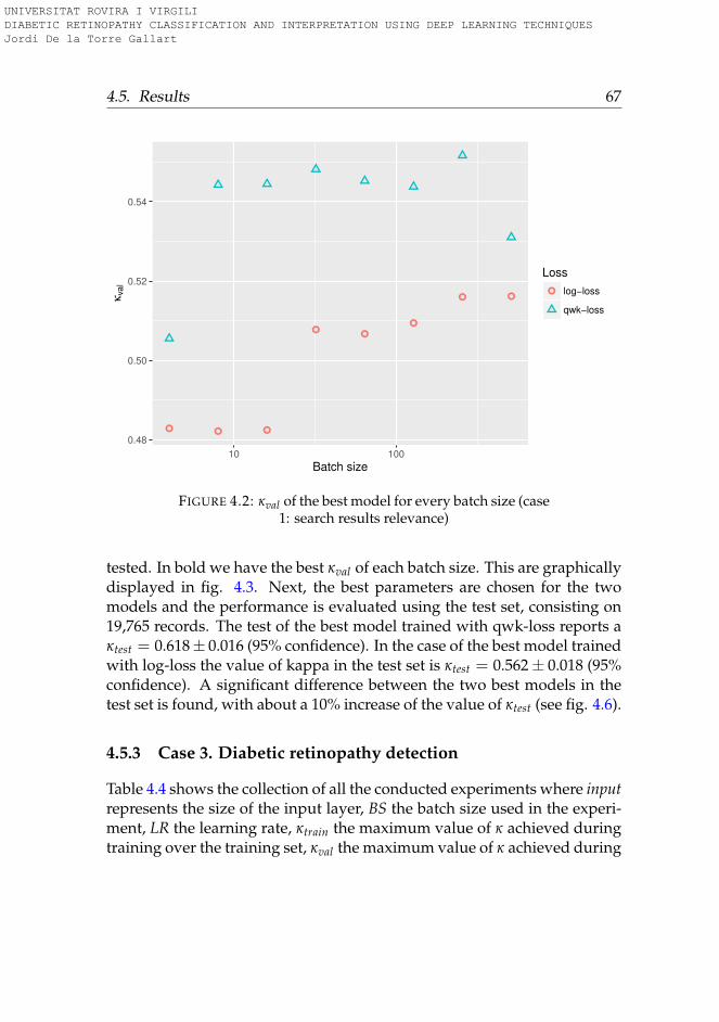
4.5. Results 67
0.48
0.50
0.52
0.54
10 100
Batch size
κval
Loss
log−loss
qwk−loss
FIGURE 4.2: κval of the best model for every batch size (case1: search results relevance)
tested. In bold we have the best κval of each batch size. This are graphicallydisplayed in fig. 4.3. Next, the best parameters are chosen for the twomodels and the performance is evaluated using the test set, consisting on19,765 records. The test of the best model trained with qwk-loss reports aκtest = 0.618± 0.016 (95% confidence). In the case of the best model trainedwith log-loss the value of kappa in the test set is κtest = 0.562± 0.018 (95%confidence). A significant difference between the two best models in thetest set is found, with about a 10% increase of the value of κtest (see fig. 4.6).
4.5.3 Case 3. Diabetic retinopathy detection
Table 4.4 shows the collection of all the conducted experiments where inputrepresents the size of the input layer, BS the batch size used in the experi-ment, LR the learning rate, κtrain the maximum value of κ achieved duringtraining over the training set, κval the maximum value of κ achieved during
UNIVERSITAT ROVIRA I VIRGILI DIABETIC RETINOPATHY CLASSIFICATION AND INTERPRETATION USING DEEP LEARNING TECHNIQUES Jordi De la Torre Gallart
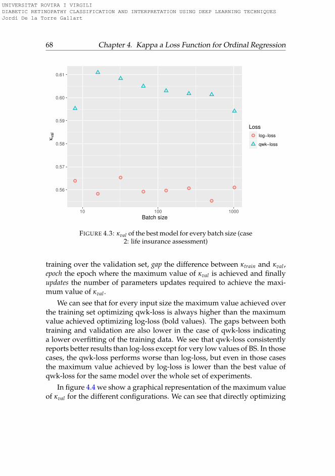
68 Chapter 4. Kappa a Loss Function for Ordinal Regression
0.56
0.57
0.58
0.59
0.60
0.61
10 100 1000
Batch size
κval
Loss
log−loss
qwk−loss
FIGURE 4.3: κval of the best model for every batch size (case2: life insurance assessment)
training over the validation set, gap the difference between κtrain and κval ,epoch the epoch where the maximum value of κval is achieved and finallyupdates the number of parameters updates required to achieve the maxi-mum value of κval .
We can see that for every input size the maximum value achieved overthe training set optimizing qwk-loss is always higher than the maximumvalue achieved optimizing log-loss (bold values). The gaps between bothtraining and validation are also lower in the case of qwk-loss indicatinga lower overfitting of the training data. We see that qwk-loss consistentlyreports better results than log-loss except for very low values of BS. In thosecases, the qwk-loss performs worse than log-loss, but even in those casesthe maximum value achieved by log-loss is lower than the best value ofqwk-loss for the same model over the whole set of experiments.
In figure 4.4 we show a graphical representation of the maximum valueof κval for the different configurations. We can see that directly optimizing
UNIVERSITAT ROVIRA I VIRGILI DIABETIC RETINOPATHY CLASSIFICATION AND INTERPRETATION USING DEEP LEARNING TECHNIQUES Jordi De la Torre Gallart
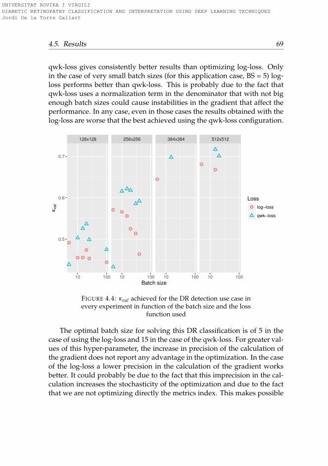
4.5. Results 69
qwk-loss gives consistently better results than optimizing log-loss. Onlyin the case of very small batch sizes (for this application case, BS = 5) log-loss performs better than qwk-loss. This is probably due to the fact thatqwk-loss uses a normalization term in the denominator that with not bigenough batch sizes could cause instabilities in the gradient that affect theperformance. In any case, even in those cases the results obtained with thelog-loss are worse that the best achieved using the qwk-loss configuration.
128x128 256x256 384x384 512x512
0.5
0.6
0.7
10 100 10 100 10 100 10 100
Batch size
κval
Loss
log−loss
qwk−loss
FIGURE 4.4: κval achieved for the DR detection use case inevery experiment in function of the batch size and the loss
function used
The optimal batch size for solving this DR classification is of 5 in thecase of using the log-loss and 15 in the case of the qwk-loss. For greater val-ues of this hyper-parameter, the increase in precision of the calculation ofthe gradient does not report any advantage in the optimization. In the caseof the log-loss a lower precision in the calculation of the gradient worksbetter. It could probably be due to the fact that this imprecision in the cal-culation increases the stochasticity of the optimization and due to the factthat we are not optimizing directly the metrics index. This makes possible
UNIVERSITAT ROVIRA I VIRGILI DIABETIC RETINOPATHY CLASSIFICATION AND INTERPRETATION USING DEEP LEARNING TECHNIQUES Jordi De la Torre Gallart
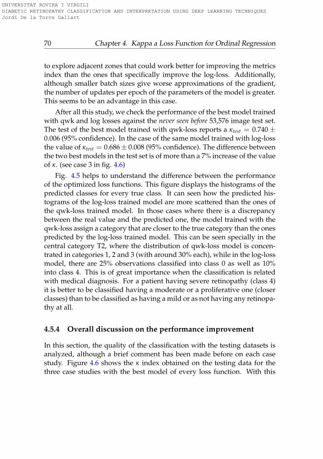
70 Chapter 4. Kappa a Loss Function for Ordinal Regression
to explore adjacent zones that could work better for improving the metricsindex than the ones that specifically improve the log-loss. Additionally,although smaller batch sizes give worse approximations of the gradient,the number of updates per epoch of the parameters of the model is greater.This seems to be an advantage in this case.
After all this study, we check the performance of the best model trainedwith qwk and log losses against the never seen before 53,576 image test set.The test of the best model trained with qwk-loss reports a κtest = 0.740±0.006 (95% confidence). In the case of the same model trained with log-lossthe value of κtest = 0.686± 0.008 (95% confidence). The difference betweenthe two best models in the test set is of more than a 7% increase of the valueof κ. (see case 3 in fig. 4.6)
Fig. 4.5 helps to understand the difference between the performanceof the optimized loss functions. This figure displays the histograms of thepredicted classes for every true class. It can seen how the predicted his-tograms of the log-loss trained model are more scattered than the ones ofthe qwk-loss trained model. In those cases where there is a discrepancybetween the real value and the predicted one, the model trained with theqwk-loss assign a category that are closer to the true category than the onespredicted by the log-loss trained model. This can be seen specially in thecentral category T2, where the distribution of qwk-loss model is concen-trated in categories 1, 2 and 3 (with around 30% each), while in the log-lossmodel, there are 25% observations classified into class 0 as well as 10%into class 4. This is of great importance when the classification is relatedwith medical diagnosis. For a patient having severe retinopathy (class 4)it is better to be classified having a moderate or a proliferative one (closerclasses) than to be classified as having a mild or as not having any retinopa-thy at all.
4.5.4 Overall discussion on the performance improvement
In this section, the quality of the classification with the testing datasets isanalyzed, although a brief comment has been made before on each casestudy. Figure 4.6 shows the κ index obtained on the testing data for thethree case studies with the best model of every loss function. With this
UNIVERSITAT ROVIRA I VIRGILI DIABETIC RETINOPATHY CLASSIFICATION AND INTERPRETATION USING DEEP LEARNING TECHNIQUES Jordi De la Torre Gallart
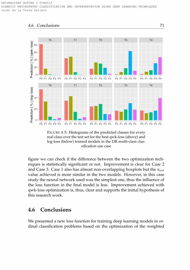
4.6. Conclusions 71
T0 T1 T2 T3 T4
0
20
40
60
80
P0 P1 P2 P3 P4 P0 P1 P2 P3 P4 P0 P1 P2 P3 P4 P0 P1 P2 P3 P4 P0 P1 P2 P3 P4
Pre
dic
tio
n [
% ]
(q
wk−
loss)
T0 T1 T2 T3 T4
0
20
40
P0 P1 P2 P3 P4 P0 P1 P2 P3 P4 P0 P1 P2 P3 P4 P0 P1 P2 P3 P4 P0 P1 P2 P3 P4
Pre
dic
tio
n [
% ]
(lo
g−
loss)
FIGURE 4.5: Histograms of the predicted classes for everyreal class over the test set for the best qwk-loss (above) andlog-loss (below) trained models in the DR multi-class clas-
sification use case
figure we can check if the difference between the two optimization tech-niques is statistically significant or not. Improvement is clear for Case 2and Case 3. Case 1 also has almost non-overlapping boxplots but the κtestvalue achieved is more similar in the two models. However, in this casestudy the neural network used was the simplest one, thus the influence ofthe loss function in the final model is less. Improvement achieved withqwk-loss optimization is, thus, clear and supports the initial hypothesis ofthis research work.
4.6 Conclusions
We presented a new loss function for training deep learning models in or-dinal classification problems based on the optimization of the weighted
UNIVERSITAT ROVIRA I VIRGILI DIABETIC RETINOPATHY CLASSIFICATION AND INTERPRETATION USING DEEP LEARNING TECHNIQUES Jordi De la Torre Gallart
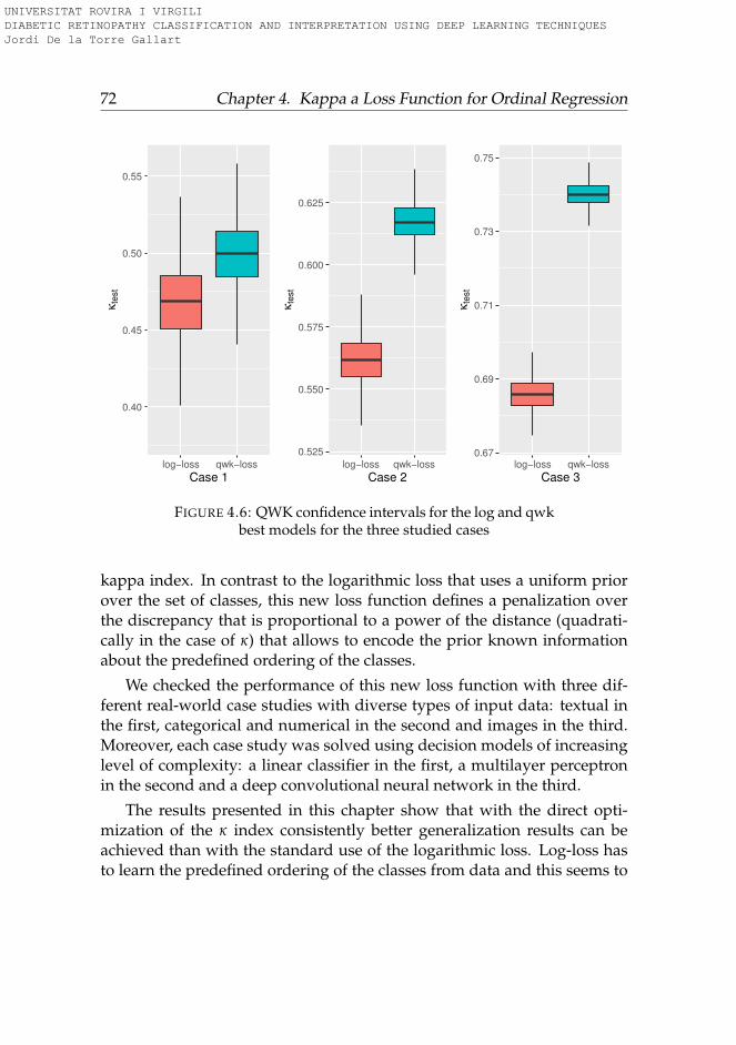
72 Chapter 4. Kappa a Loss Function for Ordinal Regression
0.40
0.45
0.50
0.55
log−loss qwk−loss
Case 1
κte
st
0.525
0.550
0.575
0.600
0.625
log−loss qwk−loss
Case 2
κte
st
0.67
0.69
0.71
0.73
0.75
log−loss qwk−loss
Case 3
κte
st
FIGURE 4.6: QWK confidence intervals for the log and qwkbest models for the three studied cases
kappa index. In contrast to the logarithmic loss that uses a uniform priorover the set of classes, this new loss function defines a penalization overthe discrepancy that is proportional to a power of the distance (quadrati-cally in the case of κ) that allows to encode the prior known informationabout the predefined ordering of the classes.
We checked the performance of this new loss function with three dif-ferent real-world case studies with diverse types of input data: textual inthe first, categorical and numerical in the second and images in the third.Moreover, each case study was solved using decision models of increasinglevel of complexity: a linear classifier in the first, a multilayer perceptronin the second and a deep convolutional neural network in the third.
The results presented in this chapter show that with the direct opti-mization of the κ index consistently better generalization results can beachieved than with the standard use of the logarithmic loss. Log-loss hasto learn the predefined ordering of the classes from data and this seems to
UNIVERSITAT ROVIRA I VIRGILI DIABETIC RETINOPATHY CLASSIFICATION AND INTERPRETATION USING DEEP LEARNING TECHNIQUES Jordi De la Torre Gallart
4.6. Conclusions 73
be a disadvantage. Results showed that, depending on the use case, be-tween 6-10% of improvement of κ scores can be obtained from the directoptimization of the function.
This is a significant improvement that may be worth in many domains,such as the one of medical diagnosis, since an accurate detection of thelevel of severity of a disease usually has great influence on the treatmentprescription and the possibility of minimizing bad consequences of the ill-ness.
One minor drawback of the new loss is its low performance with verysmall batch sizes in the image classification study. The experiments showthat for the retinopathy classification problem with batch sizes of 5, theperformance of the function is lower than using the logarithmic loss. Thisparameter is for sure problem dependent and has to be taken into accountas an important parameter to check in other image classification tasks thatuse a deep neural network.
UNIVERSITAT ROVIRA I VIRGILI DIABETIC RETINOPATHY CLASSIFICATION AND INTERPRETATION USING DEEP LEARNING TECHNIQUES Jordi De la Torre Gallart
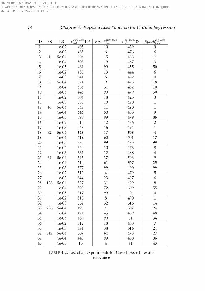
74 Chapter 4. Kappa a Loss Function for Ordinal Regression
ID BS LR κqwk-lossval 103 Epochqwk-loss
best κlog-lossval 103 Epochlog-loss
best1
4
1e-02 405 10 439 92 1e-03 485 6 476 63 5e-04 506 15 483 144 1e-04 503 19 467 35 1e-05 461 99 455 506
8
1e-02 450 13 444 67 1e-03 544 6 482 08 5e-04 524 9 475 189 1e-04 535 31 482 10
10 1e-05 445 99 479 5011
16
1e-02 504 18 425 312 1e-03 535 10 480 113 5e-04 543 11 480 114 1e-04 545 50 483 915 1e-05 395 99 479 8616
32
1e-02 515 12 436 217 1e-03 548 16 494 118 5e-04 548 17 508 419 1e-04 519 60 501 1720 1e-05 385 99 485 9921
64
1e-02 520 10 473 822 1e-03 531 12 488 423 5e-04 545 37 506 924 1e-04 514 61 507 2525 1e-05 377 99 400 9926
128
1e-02 513 4 479 527 1e-03 544 23 497 628 5e-04 527 31 499 829 1e-04 503 72 509 5530 1e-05 317 99 0 031
256
1e-02 510 8 490 132 1e-03 552 32 516 1433 5e-04 490 21 507 2434 1e-04 421 45 469 4835 1e-05 189 99 61 3436
512
1e-02 512 18 488 737 1e-03 531 38 516 2438 5e-04 509 64 493 2739 1e-04 443 99 450 8640 1e-05 15 4 41 43
TABLE 4.2: List of all experiments for Case 1: Search resultsrelevance
UNIVERSITAT ROVIRA I VIRGILI DIABETIC RETINOPATHY CLASSIFICATION AND INTERPRETATION USING DEEP LEARNING TECHNIQUES Jordi De la Torre Gallart
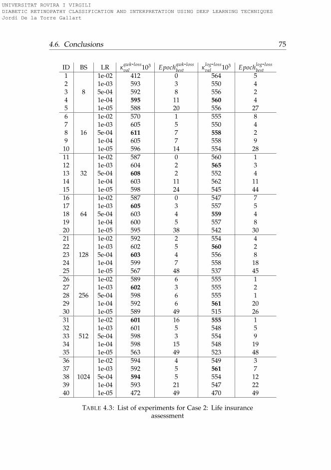
4.6. Conclusions 75
ID BS LR κqwk-lossval 103 Epochqwk-loss
best κlog-lossval 103 Epochlog-loss
best1
8
1e-02 412 0 564 52 1e-03 593 3 550 43 5e-04 592 8 556 24 1e-04 595 11 560 45 1e-05 588 20 556 276
16
1e-02 570 1 555 87 1e-03 605 5 550 48 5e-04 611 7 558 29 1e-04 605 7 558 9
10 1e-05 596 14 554 2811
32
1e-02 587 0 560 112 1e-03 604 2 565 313 5e-04 608 2 552 414 1e-04 603 11 562 1115 1e-05 598 24 545 4416
64
1e-02 587 0 547 717 1e-03 605 3 557 518 5e-04 603 4 559 419 1e-04 600 5 557 820 1e-05 595 38 542 3021
128
1e-02 592 2 554 422 1e-03 602 5 560 223 5e-04 603 4 556 824 1e-04 599 7 558 1825 1e-05 567 48 537 4526
256
1e-02 589 6 555 127 1e-03 602 3 555 228 5e-04 598 6 555 129 1e-04 592 6 561 2030 1e-05 589 49 515 2631
512
1e-02 601 16 555 132 1e-03 601 5 548 533 5e-04 598 3 554 934 1e-04 598 15 548 1935 1e-05 563 49 523 4836
1024
1e-02 594 4 549 337 1e-03 592 5 561 738 5e-04 594 5 554 1239 1e-04 593 21 547 2240 1e-05 472 49 470 49
TABLE 4.3: List of experiments for Case 2: Life insuranceassessment
UNIVERSITAT ROVIRA I VIRGILI DIABETIC RETINOPATHY CLASSIFICATION AND INTERPRETATION USING DEEP LEARNING TECHNIQUES Jordi De la Torre Gallart
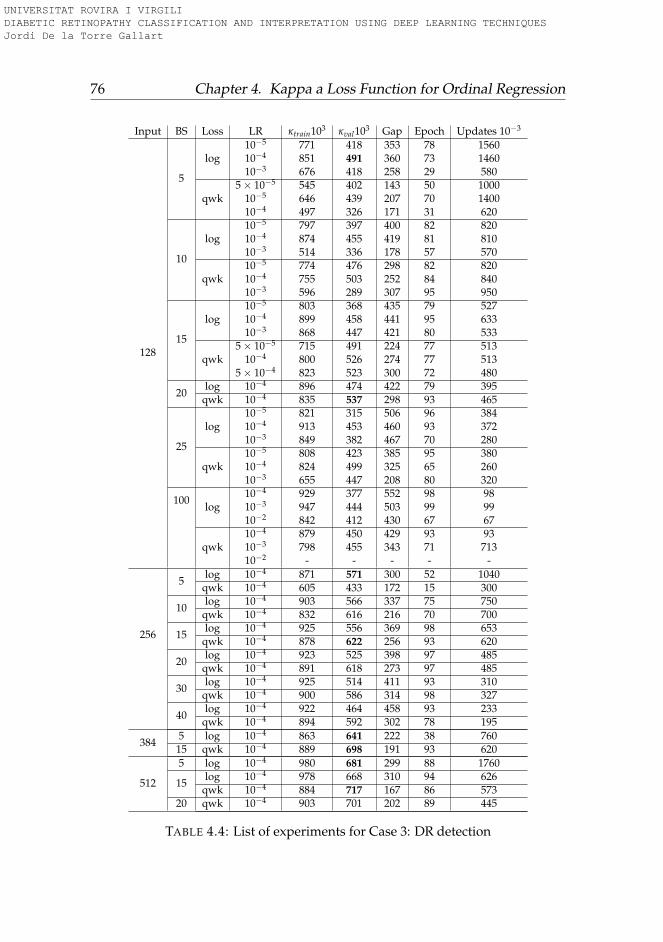
76 Chapter 4. Kappa a Loss Function for Ordinal Regression
Input BS Loss LR κtrain103 κval103 Gap Epoch Updates 10−3
128
5
log10−5 771 418 353 78 156010−4 851 491 360 73 146010−3 676 418 258 29 580
qwk5× 10−5 545 402 143 50 1000
10−5 646 439 207 70 140010−4 497 326 171 31 620
10
log10−5 797 397 400 82 82010−4 874 455 419 81 81010−3 514 336 178 57 570
qwk10−5 774 476 298 82 82010−4 755 503 252 84 84010−3 596 289 307 95 950
15
log10−5 803 368 435 79 52710−4 899 458 441 95 63310−3 868 447 421 80 533
qwk5× 10−5 715 491 224 77 513
10−4 800 526 274 77 5135× 10−4 823 523 300 72 480
20log 10−4 896 474 422 79 395
qwk 10−4 835 537 298 93 465
25
log10−5 821 315 506 96 38410−4 913 453 460 93 37210−3 849 382 467 70 280
qwk10−5 808 423 385 95 38010−4 824 499 325 65 26010−3 655 447 208 80 320
100log
10−4 929 377 552 98 9810−3 947 444 503 99 9910−2 842 412 430 67 67
qwk10−4 879 450 429 93 9310−3 798 455 343 71 71310−2 - - - - -
256
5log 10−4 871 571 300 52 1040
qwk 10−4 605 433 172 15 300
10log 10−4 903 566 337 75 750
qwk 10−4 832 616 216 70 700
15log 10−4 925 556 369 98 653
qwk 10−4 878 622 256 93 620
20log 10−4 923 525 398 97 485
qwk 10−4 891 618 273 97 485
30log 10−4 925 514 411 93 310
qwk 10−4 900 586 314 98 327
40log 10−4 922 464 458 93 233
qwk 10−4 894 592 302 78 195
3845 log 10−4 863 641 222 38 76015 qwk 10−4 889 698 191 93 620
512
5 log 10−4 980 681 299 88 1760
15log 10−4 978 668 310 94 626
qwk 10−4 884 717 167 86 57320 qwk 10−4 903 701 202 89 445
TABLE 4.4: List of experiments for Case 3: DR detection
UNIVERSITAT ROVIRA I VIRGILI DIABETIC RETINOPATHY CLASSIFICATION AND INTERPRETATION USING DEEP LEARNING TECHNIQUES Jordi De la Torre Gallart
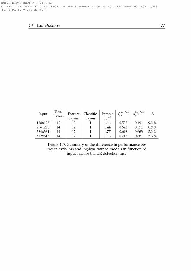
4.6. Conclusions 77
InputTotal
LayersFeatureLayers
Classific.Layers
Params10−6
κqwk-lossval κ
log-lossval ∆
128x128 12 10 1 1.16 0.537 0.491 9.3 %256x256 14 12 1 1.44 0.622 0.571 8.9 %384x384 14 12 1 1.77 0.698 0.663 5.3 %512x512 14 12 1 11.3 0.717 0.681 5.3 %
TABLE 4.5: Summary of the difference in performance be-tween qwk-loss and log-loss trained models in function of
input size for the DR detection case
UNIVERSITAT ROVIRA I VIRGILI DIABETIC RETINOPATHY CLASSIFICATION AND INTERPRETATION USING DEEP LEARNING TECHNIQUES Jordi De la Torre Gallart

UNIVERSITAT ROVIRA I VIRGILI DIABETIC RETINOPATHY CLASSIFICATION AND INTERPRETATION USING DEEP LEARNING TECHNIQUES Jordi De la Torre Gallart
79
Chapter 5
Enhanced Models
In this chapter we present a part of the work published in (Torre, Valls, andPuig, 2017). Concretely, the optimized classification model for DR diseasegrading. The model presented here has a statistically proven ophthalmol-ogist level performance, reaching a inter-rating agreement in never-seen-before Messidor dataset of QWK = 0.83, with a unique evaluation and noensembling.
5.1 Introduction
Deep Learning (DL) methods (Lecun, Bengio, and Hinton, 2015), (Schmid-huber, 2015) have been extensively used in the last years for many auto-matic classification tasks. For the case of image classification, the usualprocedure consists on extracting the important features using a set of con-volutional layers and, after that, make a final classification with these fea-tures using a set of fully connected layers. At the end, a soft-max outputlayer gives the predicted output probabilities of belonging to the classespredefined in the model. During training, model parameters are changedusing a gradient-based optimization algorithm, which minimizes a prede-fined loss function.(Goodfellow, Bengio, and Courville, 2016)
Once the classifier has been trained (i.e. model layer parameters havebeen fixed), the quality of the classification output is compared against thecorrect "true" values stored on a labeled dataset. This data is considered asthe gold standard, ideally coming from the consensus of the knowledge ofa committee of human experts.
UNIVERSITAT ROVIRA I VIRGILI DIABETIC RETINOPATHY CLASSIFICATION AND INTERPRETATION USING DEEP LEARNING TECHNIQUES Jordi De la Torre Gallart
80 Chapter 5. Enhanced Models
This mapping allows the classification of multi-dimensional objects intoa small number of categories. The model is composed by many neuronsthat are organized in layers and blocks of layers, piled together in a hi-erarchical way. Every neuron receives the input from a predefined set ofneurons. In addition, every connection has a parameter that correspondsto the weight of the relation.
The function of every neuron is to make a transformation of the re-ceived inputs into a calculated output value. For each incoming connec-tion, a weight is multiplied by the input value and the aggregation overall inputs is fed to an activation function that calculates the neuron out-put. Parameters are usually optimized using a stochastic gradient descentalgorithm that minimizes a predefined loss function. Network parametersare updated after back-propagating the loss function gradients through thenetwork. These hierarchical models are able to learn multiple levels ofrepresentation that correspond to different levels of abstraction, which en-ables the representation of complex concepts in a compressed way (Bengio,Courville, and Vincent, 2013), (Bengio, 2009).
The first successful convolutional neural network (CNN) published (Le-Cun et al., 1998) was designed for hand-written digit recognition. Thisearly CNN implementation used a combination of convolution, poolingand non-linearity that has been the key feature of DL until now. It usedconvolutions for extracting spatial features, sub-sampling for reducing mapssize, a non-linearity in the form of tanh or sigmoids, and a fully connectedmulti-layer neural network as final classifier. Network parameters were alllearned using an end-to-end optimization algorithm using stochastic gra-dient descent. One of the first successful implementations using GPUs waspublished in (Ciresan et al., 2010) where they successfully trained a neu-ral network with 9 layers, also for handwritten digit recognition. The DLbreakthrough took place with the publication of (Krizhevsky, Sutskever,and Hinton, 2012a) where, for the first time, a CNN won the Imagenet(Denget al., 2009) classification competition by a large margin. The network,named AlexNet, introduced a set of innovative techniques like data aug-mentation, the use of rectified linear units (ReLUs) as non-linearities, theuse of dropout for avoiding overfitting, overlapping max-pooling avoidingthe averaging effects of avg-pooling and the use of GPUs for speeding upthe training time. This paper proved experimentally that CNNs were able
UNIVERSITAT ROVIRA I VIRGILI DIABETIC RETINOPATHY CLASSIFICATION AND INTERPRETATION USING DEEP LEARNING TECHNIQUES Jordi De la Torre Gallart
5.1. Introduction 81
to solve complex tasks. From the publication of this paper many improve-ments where published, like (Sermanet et al., 2014) with the introductionof Overfeat, a network derivation of AlexNet where they proposed learn-ing bounding boxes, which later gave rise to many other papers on thesame topic. In (Simonyan and Zisserman, 2015), VGG networks wherepresented. It was the first time that small 3x3 convolution filters whereused and combined as a sequence of convolutions. The previous big filtersof 9x9 and 11x11 present in AlexNet started to become smaller. The greatadvantage of VGG network was the insight of stacking 3x3 convolutionsas a substitution of large filters. These ideas were used in the design ofposterior networks like ResNet and Inception. GoogleNet(Szegedy et al.,2015) and Inception (Szegedy et al., 2016) were the first attempts to reducethe size of big networks. DL was becoming very useful for categorizationof images and video frames, but its main concern was its low efficiency insize and computation. Inception module used a parallel calculation of 1x1,3x3 and 5x5 convolutions significantly reducing the number of operationsrequired by networks like AlexNet and VGG. Bottleneck layers (1x1 con-volutions) where used before the calculation of bigger size convolutionsfor reducing the number of input filters, reducing in this way the compu-tational costs without losing generality. So, 1x1 convolutions have beenproven to achieve state-of-the-art results in Imagenet classification tasks.The reason of this success is that input features are correlated, being re-moved by combining them appropriately with the 1x1 convolutions. Then,after convolution with a smaller number of features, they can be expandedagain into a meaningful combination for the next layer. Another revolutioncame with the introduction of residual networks in (He et al., 2016). Thesenetworks used a combination of 3x3 convolutional layers with a by-passof the input every two layers that was summed up to the output. The in-troduction of such bypass improved the gradient propagation through thenetwork allowing the use of deeper networks and improving the classifica-tion capabilities. In (Szegedy et al., 2017), a modified version of Inceptionnetworks called InceptionResNet was published to introduce this idea tosuch networks. Residual blocks allowed the reduction of training time, notimproving significantly the classification performance.
DL models have been also successfully applied in many medical clas-sification tasks. In (Esteva et al., 2017) a DL classifier was designed achiev-ing dermatologist-level accuracy for skin cancer detection. In (Zhu et al.,
UNIVERSITAT ROVIRA I VIRGILI DIABETIC RETINOPATHY CLASSIFICATION AND INTERPRETATION USING DEEP LEARNING TECHNIQUES Jordi De la Torre Gallart
82 Chapter 5. Enhanced Models
2018) a 3D CNN for automated pulmonary nodule detection and classifica-tion was built. In (Wang et al., 2018) a CNN Alzheimer’s disease classifierwith high performance was also described. In (Gulshan, Peng, and Coram,2016) the authors presented a DR classifier with better performance thanhuman experts in the detection of the most severe cases of the disease.
5.2 Related work
Many deep learning classifiers for DR have been published in the last years.In (Torre, Puig, and Valls, 2018) a DL classifier was published for the pre-diction of the different disease grades. This model was trained using thepublic available EyePACS dataset. The training set had 35,126 images andthe test set 53,576. The quadratic weighted kappa (QWK) evaluation met-ric (Cohen, 1968) was close to the reported by human experts in the test setusing a unique DL model without ensembling.
In (Gulshan, Peng, and Coram, 2016) a binary DL classifier was pub-lished for the detection of the most severe cases of DR (grouping classes 0and 1 of DR on one side, and classes 2, 3 and 4 on another). This modelwas trained using an extended version of the EyePACS dataset mentionedbefore with a total of 128,175 images and improving the proper taggingof the images using a set of 3 to 7 experts chosen from a panel of 54 USexpert ophthalmologists. This model surpassed the human expert capa-bilities, reaching approximately a performance of 97% in sensitivity and93.5% in specificity in test sets of about 10,000 images. The strength of thismodel was its ability to predict the more severe cases with a sensitivity andspecificity greater than human experts. The drawback, as many DL basedmodels, is its lack of interpretability. The model acts like a intuition machinewith a highly statistical confidence but lacking an interpretation of the ra-tionale behind the decisions, making difficult to the experts to have cluesto improve the diagnostics.
UNIVERSITAT ROVIRA I VIRGILI DIABETIC RETINOPATHY CLASSIFICATION AND INTERPRETATION USING DEEP LEARNING TECHNIQUES Jordi De la Torre Gallart
5.3. Classification model for DR 83
5.3 Classification model for DR
5.3.1 Data
We use the EyePACS dataset presented in chapter 2. The dataset is splitinto two disjoint sets containing eye images of different patients, one fortraining and the other for testing.
The training set contains a total of 75, 650 images; 55, 796 of class 0,5, 259 of class 1, 11, 192 of class 2, 1, 805 of class 3 and 1, 598 of class 4. Thevalidation set used for hyper-parameter optimization has 3, 000 images;2, 150 of class 0, 209 of class 1, 490 of class 2, 61 of class 3 and 90 of class 4.
The test set contains a total of 10, 000 images of patients not present intraining set; 7, 363 of class 0, 731 of class 1, 1, 461 of class 2, 220 of class 3and 225 of class 4.
This dataset is not so rich and well tagged as the used in (Gulshan,Peng, and Coram, 2016) but allows to train models near human expertisethat are useful to show the purposes of our work, which is not only a goodperformance of the classification results but mainly to provide tools forinterpretability of the final classification of each patient.
5.3.2 Construction of the classifier
The model calculates the probability P(C|I), being C one of the possibleoutput classes and I the retina image. Using as a last layer a So f tMaxfunction over the values after the last linear combination of features. Thisprobability is calculated as P(C|I) = eSi
∑Cj=1 eSj
. Let us call SC the score of
class C, being SC the final value of each output neuron before applying theSo f tmax. So f tmax function is required for calculating the probability of ev-ery class, but in case of being interested only on argmax(So f tmax), we donot need evaluate So f tmax because argmax(Si) = argmax(So f tmax(Si)).Thus, we skip So f tmax from the interpretation analysis.
UNIVERSITAT ROVIRA I VIRGILI DIABETIC RETINOPATHY CLASSIFICATION AND INTERPRETATION USING DEEP LEARNING TECHNIQUES Jordi De la Torre Gallart
84 Chapter 5. Enhanced Models
Design guidelines for DR classification
Up to now, the design of deep neural network models is mainly driven byexperience. Nowadays it is still more an art than a science and lacks a sys-tematic way for designing the best architecture for solving a problem. Inprevious works (see (Torre, Valls, and Puig, 2016a) and (Torre, Puig, andValls, 2018)), we have tested different kinds of architectures for DR clas-sification. Using the previous experience in such works we report here aset of guidelines that have been used to build the proposed classificationmodel for DR. These design principles for DR classification can be summa-rized into: use an optimal image resolution, use all the image informationavailable, use a fully CNN, use small convolutions, adapt the combinationof convolution sizes and number of layers to have a final RF as similaras possible to the image size, use ReLU as activation function, use batchnormalization in every layer, use QWK as a loss function, use a efficientnumber of features and use a linear classifier as the last layer.
Use an optimal image resolution On the one hand, image input size hasa great importance in the classification results. For this problem, other pa-pers like (Torre, Valls, and Puig, 2016a) have shown that better results canbe achieved with retina diameters of 512 pixels than with 384, 256 or 128pixels. Some tests done using densities larger than 512 pixel/diameterseem to not improve significantly the classification rates. On the otherhand, the hardware of calculation devices fix a limitation on the availableresources. Input image size has a great impact on the memory and calcu-lation time required for the training and test of the deep neural networkmodels. For this present work, we tested models of 128, 256, 384, 512, 640,724, 768 and 892 pixels of retina diameter. With this dataset, diametersgreater than 640 does not seem to report better results. The optimal size isa retina diameter equal to 640 pixels. This is the one used for the resultsshown in this chapter.
Use all the available image information In previous studies publishedin (Torre, Valls, and Puig, 2016a), due to hardware limitations, the classifi-cation models were designed using limited input information, using onlypart of the available input, requiring ensembling solutions to combine the
UNIVERSITAT ROVIRA I VIRGILI DIABETIC RETINOPATHY CLASSIFICATION AND INTERPRETATION USING DEEP LEARNING TECHNIQUES Jordi De la Torre Gallart
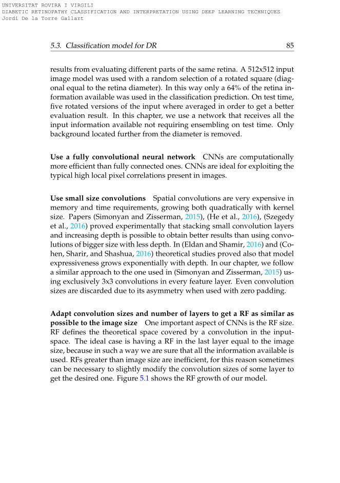
5.3. Classification model for DR 85
results from evaluating different parts of the same retina. A 512x512 inputimage model was used with a random selection of a rotated square (diag-onal equal to the retina diameter). In this way only a 64% of the retina in-formation available was used in the classification prediction. On test time,five rotated versions of the input where averaged in order to get a betterevaluation result. In this chapter, we use a network that receives all theinput information available not requiring ensembling on test time. Onlybackground located further from the diameter is removed.
Use a fully convolutional neural network CNNs are computationallymore efficient than fully connected ones. CNNs are ideal for exploiting thetypical high local pixel correlations present in images.
Use small size convolutions Spatial convolutions are very expensive inmemory and time requirements, growing both quadratically with kernelsize. Papers (Simonyan and Zisserman, 2015), (He et al., 2016), (Szegedyet al., 2016) proved experimentally that stacking small convolution layersand increasing depth is possible to obtain better results than using convo-lutions of bigger size with less depth. In (Eldan and Shamir, 2016) and (Co-hen, Sharir, and Shashua, 2016) theoretical studies proved also that modelexpressiveness grows exponentially with depth. In our chapter, we followa similar approach to the one used in (Simonyan and Zisserman, 2015) us-ing exclusively 3x3 convolutions in every feature layer. Even convolutionsizes are discarded due to its asymmetry when used with zero padding.
Adapt convolution sizes and number of layers to get a RF as similar aspossible to the image size One important aspect of CNNs is the RF size.RF defines the theoretical space covered by a convolution in the input-space. The ideal case is having a RF in the last layer equal to the imagesize, because in such a way we are sure that all the information available isused. RFs greater than image size are inefficient, for this reason sometimescan be necessary to slightly modify the convolution sizes of some layer toget the desired one. Figure 5.1 shows the RF growth of our model.
UNIVERSITAT ROVIRA I VIRGILI DIABETIC RETINOPATHY CLASSIFICATION AND INTERPRETATION USING DEEP LEARNING TECHNIQUES Jordi De la Torre Gallart
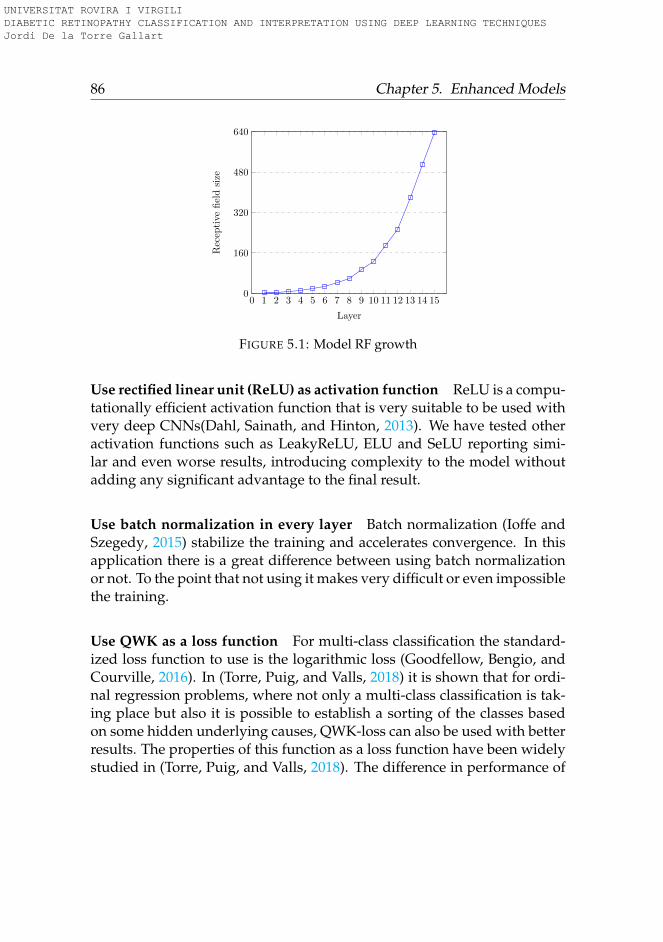
86 Chapter 5. Enhanced Models
0 1 2 3 4 5 6 7 8 9 10 11 12 13 14 150
160
320
480
640
Layer
Rec
epti
vefi
eld
size
FIGURE 5.1: Model RF growth
Use rectified linear unit (ReLU) as activation function ReLU is a compu-tationally efficient activation function that is very suitable to be used withvery deep CNNs(Dahl, Sainath, and Hinton, 2013). We have tested otheractivation functions such as LeakyReLU, ELU and SeLU reporting simi-lar and even worse results, introducing complexity to the model withoutadding any significant advantage to the final result.
Use batch normalization in every layer Batch normalization (Ioffe andSzegedy, 2015) stabilize the training and accelerates convergence. In thisapplication there is a great difference between using batch normalizationor not. To the point that not using it makes very difficult or even impossiblethe training.
Use QWK as a loss function For multi-class classification the standard-ized loss function to use is the logarithmic loss (Goodfellow, Bengio, andCourville, 2016). In (Torre, Puig, and Valls, 2018) it is shown that for ordi-nal regression problems, where not only a multi-class classification is tak-ing place but also it is possible to establish a sorting of the classes basedon some hidden underlying causes, QWK-loss can also be used with betterresults. The properties of this function as a loss function have been widelystudied in (Torre, Puig, and Valls, 2018). The difference in performance of
UNIVERSITAT ROVIRA I VIRGILI DIABETIC RETINOPATHY CLASSIFICATION AND INTERPRETATION USING DEEP LEARNING TECHNIQUES Jordi De la Torre Gallart
5.3. Classification model for DR 87
the final results is very high. Optimizing directly QWK allows achievingbetter classification results.
Use a linear classifier as a last layer For simplicity and interpretability,we expect the model to disentangle completely the features required forthe classification. Final classification is required to be done using a linearcombination of last layer features.
0 16 32 48 630
25
50
75
100
Feature
%varian
ceexplained
FIGURE 5.2: Feature space cummulative PCA variance oftraining set
Use a efficient number of features With infinitely number of resourceswe can use a big network. In our project we have limited device resources.In addition, we would like to be able to implement the result in deviceswith low resources too. Having this in mind, we tested networks of dif-ferent sizes. In order to check the redundancy of information, we made aprincipal component analysis (PCA) in the feature space of the last layer,arriving to the conclusion that about 32 of the features explain 98.3 % and48 features, 99.997% of the total variance. We studied different configu-rations using different number of features from 512 to 32. Values of 32showed a reduction in performance that increased when using 64 features.Higher number of features did not improve the results. In figure 5.2 weshow the variance explained by the 64 feature vector space.
UNIVERSITAT ROVIRA I VIRGILI DIABETIC RETINOPATHY CLASSIFICATION AND INTERPRETATION USING DEEP LEARNING TECHNIQUES Jordi De la Torre Gallart
88 Chapter 5. Enhanced Models
Classification model description
Following the given guidelines, our model uses a 3x640x640 input imageobtained from a minimal preprocessing step, where only the external back-ground borders are trimmed and later resized to the required input size.Figure 5.3 shows a block diagram of the model. It is a CNN with 391,325parameters, divided in 17 layers. Layers are divided into two groups: thefeature extractor and the classifier. The feature extraction has 7 blocks of2 layers. Every layer is a stack of a 3x3 convolution with stride 1x1 andpadding 1x1 followed by a batch normalization and a ReLU activationfunction. Between every block a 2x2 max-pooling operation of stride 2x2 isapplied. After the 7 blocks of feature extraction, the RF of the network hasgrown till reaching 637x637, that is approximately equal to the input size640x640 (see fig 5.1 to see the RF of every layer). Afterwards, the classifi-cation phase takes place using a 2x2 convolution. A 4x4 average-poolingreduces the dimensionality to get a final 64 feature vector that are linearlycombined to obtain the output scores of every class. A soft-max functionallows the conversion of scores to probabilities to feed the values to theproper cost function during the optimization process. The feature extrac-tor has 16 filters in the first block, 32 in the second and 64 in all the other.
5.3.3 Training procedure
As presented in section 5.3.1, the training set training set has 75,650 imagesand the validation set used for hyper-parameter selection 3,000. Noticethat the image set is highly imbalanced. In order to facilitate the learning,the training set is artificially equalized using data augmentation techniques(Krizhevsky, Sutskever, and Hinton, 2012b) based on 0− 180◦ random ro-tation, X and Y mirroring and contrast&brightness random sampling.
A random initialization based in the Kaiming&He approach (He et al.,2015) is used. All models are optimized using a batch based first order opti-mization algorithm called Adam (Kingma and Ba, 2014). The loss functionused for optimizing the model is the QWK-loss function, with a batch sizeof 15 and a learning rate of 3x10⁻⁴ (Torre, Puig, and Valls, 2018). For everybatch, the images are chosen randomly from the training set, with repeti-tion.
UNIVERSITAT ROVIRA I VIRGILI DIABETIC RETINOPATHY CLASSIFICATION AND INTERPRETATION USING DEEP LEARNING TECHNIQUES Jordi De la Torre Gallart
5.4. Results 89
After network training, a linear classifier formed by the combinationof the 128 features of the two eyes of the patient is trained. In this way ispossible to increase further the prediction performance of the model usingall the information available of the patient.
5.4 Results
The model is trained for 300 epochs, reaching a QWK value of 0.814 onthe validation set. The value achieved in the testing set (with images notused in the training) of 10,000 images is of 0.801. Using a linear classifier forcombining the features of both eyes QWKtest, we can reach a QWK value of0.844. Expert ophthalmologist report QWK inter-rating agreement valuesclose to 0.80.
If we consider a binary classification with two categories, one for severecases of DR (grouping classes 2, 3 and 4) and another for non-sever cases(classes 0 and 1), we can calculate the usual classification evaluation met-rics. Over EyePACS test set we obtain the following values for differentmeasures1: N=10,000, TP=1,727, TN=6,859, FP=1,235, FN=179, Sensitiv-ity=0.906 (95% CI: 0.893 to 0.919), Specificity=0.847 (95% CI: 0.840-0.855),PPV=0.583, NPV=0.975, Accuracy=0.857, F1=0.710 and MCC=0.648.
For comparison purposes with other works, we tested also our modelagainst the standardised Messidor-2 dataset (Decencière et al., 2014). Weachieve a QWK of 0.832 for this dataset. Binary classification statistics forprediction of the most severe cases of DR (grouping classes 2, 3 and macu-lar edema) are: N=1200, TP=465, TN=627, FP=61, FN=47, Sensitivity=0.908(95% CI: 0.883 to 0.933), Specificity=0.911 (95% CI: 0.890-0.933), PPV=0.884,NPV=0.930, Accuracy=0.910, F1=0.896 and MCC=0.817.
We can see that the results obtained with the Messidor-2 dataset arebetter because of the improved quality of images in the dataset and a alsoa better labelling of the examples.
In order to compare our model with state-of-the-art (Gulshan, Peng,and Coram, 2016), table 5.1 show statistics for prediction of the most severe
1 Notation: N: sample size, TP: true positives, TN: true negatives, FP: false positives,FN: false negatives, CI: confidence interval, PPV: positive predictive value, NPV: negativepredictive value, F1: F1 score and MCC: Matthews correlation coefficient
UNIVERSITAT ROVIRA I VIRGILI DIABETIC RETINOPATHY CLASSIFICATION AND INTERPRETATION USING DEEP LEARNING TECHNIQUES Jordi De la Torre Gallart
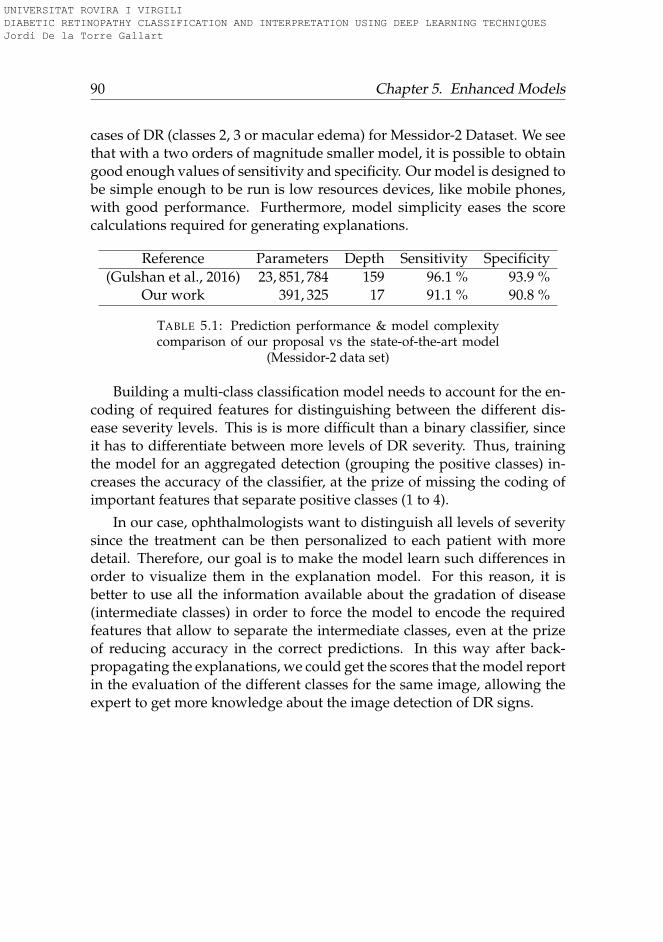
90 Chapter 5. Enhanced Models
cases of DR (classes 2, 3 or macular edema) for Messidor-2 Dataset. We seethat with a two orders of magnitude smaller model, it is possible to obtaingood enough values of sensitivity and specificity. Our model is designed tobe simple enough to be run is low resources devices, like mobile phones,with good performance. Furthermore, model simplicity eases the scorecalculations required for generating explanations.
Reference Parameters Depth Sensitivity Specificity(Gulshan et al., 2016) 23, 851, 784 159 96.1 % 93.9 %
Our work 391, 325 17 91.1 % 90.8 %
TABLE 5.1: Prediction performance & model complexitycomparison of our proposal vs the state-of-the-art model
(Messidor-2 data set)
Building a multi-class classification model needs to account for the en-coding of required features for distinguishing between the different dis-ease severity levels. This is is more difficult than a binary classifier, sinceit has to differentiate between more levels of DR severity. Thus, trainingthe model for an aggregated detection (grouping the positive classes) in-creases the accuracy of the classifier, at the prize of missing the coding ofimportant features that separate positive classes (1 to 4).
In our case, ophthalmologists want to distinguish all levels of severitysince the treatment can be then personalized to each patient with moredetail. Therefore, our goal is to make the model learn such differences inorder to visualize them in the explanation model. For this reason, it isbetter to use all the information available about the gradation of disease(intermediate classes) in order to force the model to encode the requiredfeatures that allow to separate the intermediate classes, even at the prizeof reducing accuracy in the correct predictions. In this way after back-propagating the explanations, we could get the scores that the model reportin the evaluation of the different classes for the same image, allowing theexpert to get more knowledge about the image detection of DR signs.
UNIVERSITAT ROVIRA I VIRGILI DIABETIC RETINOPATHY CLASSIFICATION AND INTERPRETATION USING DEEP LEARNING TECHNIQUES Jordi De la Torre Gallart
5.5. Conclusions 91
5.5 Conclusions
We designed a model for DR classification, reaching more than 90% of sen-sitivity and specificity for the detection of the more severe cases of DR,not far from the state-of-the-art solution with two orders of magnitude lessparameters. The designed model is also able to differentiate between thefive standardized levels of disease severity, achieving in the test set of theEyePACS dataset a quadratic weighted kappa of 0.80 with the informationof one eye and of 0.844 using the information coming from both eyes. Inthe Messidor-2 dataset the value of QWK achieved is of 0.83 using only theinformation of one eye. In all cases, the achieved performance is similar oreven better than the reported by experts ophthalmologists, that is also near0.80.
UNIVERSITAT ROVIRA I VIRGILI DIABETIC RETINOPATHY CLASSIFICATION AND INTERPRETATION USING DEEP LEARNING TECHNIQUES Jordi De la Torre Gallart
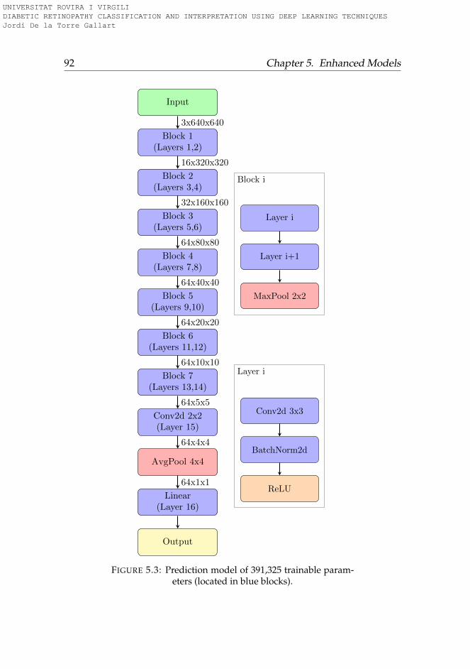
92 Chapter 5. Enhanced Models
Input
Block 1(Layers 1,2)
Block 2(Layers 3,4)
Block 3(Layers 5,6)
Block 4(Layers 7,8)
Block 5(Layers 9,10)
Block 6(Layers 11,12)
Block 7(Layers 13,14)
Conv2d 2x2(Layer 15)
AvgPool 4x4
Linear(Layer 16)
Output
3x640x640
16x320x320
32x160x160
64x80x80
64x40x40
64x20x20
64x10x10
64x5x5
64x4x4
64x1x1
Block i
Layer i
Layer i+1
MaxPool 2x2
Layer i
Conv2d 3x3
BatchNorm2d
ReLU
FIGURE 5.3: Prediction model of 391,325 trainable param-eters (located in blue blocks).
UNIVERSITAT ROVIRA I VIRGILI DIABETIC RETINOPATHY CLASSIFICATION AND INTERPRETATION USING DEEP LEARNING TECHNIQUES Jordi De la Torre Gallart
93
Chapter 6
Classification Stability
In this chapter we present a stability study done using our best perfor-mance algorithm. Deep learning models act many times as black box pre-diction machines that are trained using, many times, a large but finite train-ing set. The purpose of the analysis presented in this chapter is study howthe prediction capabilities of the model are affected by changes in the prop-erties of input images. Learning about this behavior gives a better under-standing of the robustness and limitations of the designed model.
6.1 Introduction
Deep learning models are trained using an end-to-end automatic processthat allows to learn the best internal representation (ie. the features andthe optimal classifier) minimizing a predefined loss function. As a result,an optimal parameterized model is obtained. Such models typically havehundreds of thousands or millions of parameters, being difficult to inter-pret. The model validity is tested using a test data set hopefully comingfrom the same data distribution that the training set. Using a big enoughtest set of never seen before data, it is possible to corroborate the statisti-cal validity of the results reported by the model. Such type of test givesus a overall understanding about the statistical performance, however itdoes not give us any information about the model behavior under varia-tion of typical input image parameters like rotation, lightness, hue, satura-tion, zoom, etc.
The purpose of this chapter is the study of results variability under
UNIVERSITAT ROVIRA I VIRGILI DIABETIC RETINOPATHY CLASSIFICATION AND INTERPRETATION USING DEEP LEARNING TECHNIQUES Jordi De la Torre Gallart
94 Chapter 6. Classification Stability
typical changes in the input image parameters. This study allows a bet-ter understanding of the nature of trained models in order to increase itsrobustness and to know the intrinsic limitations of the trained models.
6.2 Methods
First of all, the method used for testing model robustness consists on defin-ing set of parameters that are considered important to test. For all the setof parameters an interval of variation is defined. For a set of images, rep-resentative of the population of study, new images are generated with thenew parameters defined. Classification scores are calculated for every newimage generated and a graphical representation of classification scores ver-sus parameter values are also generated. With such plots it is possible thedetermine the stability of model results under typical variations of the in-put properties.
The image parameters that are studied in this chapter are: rotation,lightness, hue and saturation.
Rotation: The model of study have been trained using data augmen-tation techniques that included random rotation. Therefore, the modelshould be robust to changes in image input rotation. Testing against suchproperty will help us decide if multiple evaluations using different inputrotated versions are required and also if results are seriously affected tochanges of this variable or not. For each image, 360 evaluations have beendone using different rotated versions of the same image, each one sepa-rated by 1 degree of rotation.
Hue, Lightness and Saturation: The model uses as input a 3 channelsred, green, blue (RGB) representation of the retina image. From a con-ceptual perspective, color space is sometimes better to be considered us-ing another type of representation, ie. hue, lightness and saturation (HLS)color space (see figure 6.1). HLS aligns better with the way human visionperceives color-making attributes. Lightness representing the brightnessrelative to the brightness of a similarly illuminated white; hue referring tothe attribute of a visual sensation according to which an area appears to be
UNIVERSITAT ROVIRA I VIRGILI DIABETIC RETINOPATHY CLASSIFICATION AND INTERPRETATION USING DEEP LEARNING TECHNIQUES Jordi De la Torre Gallart
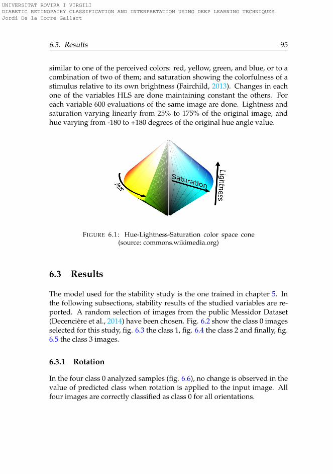
6.3. Results 95
similar to one of the perceived colors: red, yellow, green, and blue, or to acombination of two of them; and saturation showing the colorfulness of astimulus relative to its own brightness (Fairchild, 2013). Changes in eachone of the variables HLS are done maintaining constant the others. Foreach variable 600 evaluations of the same image are done. Lightness andsaturation varying linearly from 25% to 175% of the original image, andhue varying from -180 to +180 degrees of the original hue angle value.
FIGURE 6.1: Hue-Lightness-Saturation color space cone(source: commons.wikimedia.org)
6.3 Results
The model used for the stability study is the one trained in chapter 5. Inthe following subsections, stability results of the studied variables are re-ported. A random selection of images from the public Messidor Dataset(Decencière et al., 2014) have been chosen. Fig. 6.2 show the class 0 imagesselected for this study, fig. 6.3 the class 1, fig. 6.4 the class 2 and finally, fig.6.5 the class 3 images.
6.3.1 Rotation
In the four class 0 analyzed samples (fig. 6.6), no change is observed in thevalue of predicted class when rotation is applied to the input image. Allfour images are correctly classified as class 0 for all orientations.
UNIVERSITAT ROVIRA I VIRGILI DIABETIC RETINOPATHY CLASSIFICATION AND INTERPRETATION USING DEEP LEARNING TECHNIQUES Jordi De la Torre Gallart
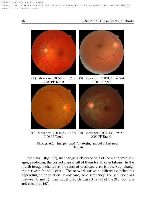
96 Chapter 6. Classification Stability
(A) Messidor 20051020 625100100 PP Tag: 0
(B) Messidor 20060523 455240100 PP Tag: 0
(C) Messidor 20060523 487090100 PP Tag: 0
(D) Messidor 20051130 590290400 PP Tag: 0
FIGURE 6.2: Images used for testing model robustness(Tag: 0)
For class 1 (fig. 6.7), no change is observed in 3 of the 4 analyzed im-ages, predicting the correct class in all of them for all orientations. In thefourth image a change in the score of predicted class is observed, chang-ing between 0 and 1 class. The network arrive to different conclusionsdepending on orientation. In any case, the discrepancy is only of one class(between 0 and 1). The model predicts class 0 in 193 of the 360 rotationsand class 1 in 167.
UNIVERSITAT ROVIRA I VIRGILI DIABETIC RETINOPATHY CLASSIFICATION AND INTERPRETATION USING DEEP LEARNING TECHNIQUES Jordi De la Torre Gallart
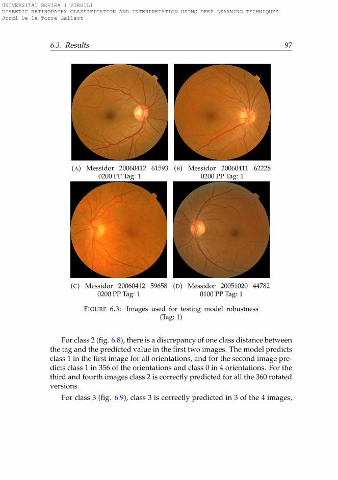
6.3. Results 97
(A) Messidor 20060412 615930200 PP Tag: 1
(B) Messidor 20060411 622280200 PP Tag: 1
(C) Messidor 20060412 596580200 PP Tag: 1
(D) Messidor 20051020 447820100 PP Tag: 1
FIGURE 6.3: Images used for testing model robustness(Tag: 1)
For class 2 (fig. 6.8), there is a discrepancy of one class distance betweenthe tag and the predicted value in the first two images. The model predictsclass 1 in the first image for all orientations, and for the second image pre-dicts class 1 in 356 of the orientations and class 0 in 4 orientations. For thethird and fourth images class 2 is correctly predicted for all the 360 rotatedversions.
For class 3 (fig. 6.9), class 3 is correctly predicted in 3 of the 4 images,
UNIVERSITAT ROVIRA I VIRGILI DIABETIC RETINOPATHY CLASSIFICATION AND INTERPRETATION USING DEEP LEARNING TECHNIQUES Jordi De la Torre Gallart
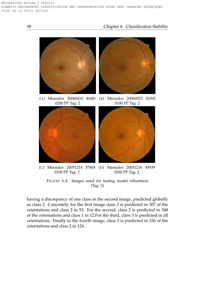
98 Chapter 6. Classification Stability
(A) Messidor 20060410 404810200 PP Tag: 2
(B) Messidor 20060523 503920100 PP Tag: 2
(C) Messidor 20051214 574040100 PP Tag: 2
(D) Messidor 20051216 449390200 PP Tag: 2
FIGURE 6.4: Images used for testing model robustness(Tag: 2)
having a discrepancy of one class in the second image, predicted globallyas class 2. Concretely, for the first image class 3 is predicted in 307 of theorientations and class 2 in 53. For the second, class 2 is predicted in 348of the orientations and class 1 in 12.For the third, class 3 is predicted in allorientations. Finally in the fourth image, class 3 is predicted in 236 of theorientations and class 2 in 124.
UNIVERSITAT ROVIRA I VIRGILI DIABETIC RETINOPATHY CLASSIFICATION AND INTERPRETATION USING DEEP LEARNING TECHNIQUES Jordi De la Torre Gallart
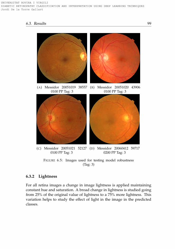
6.3. Results 99
(A) Messidor 20051019 385570100 PP Tag: 3
(B) Messidor 20051020 439060100 PP Tag: 3
(C) Messidor 20051021 521270100 PP Tag: 3
(D) Messidor 20060412 597170200 PP Tag: 3
FIGURE 6.5: Images used for testing model robustness(Tag: 3)
6.3.2 Lightness
For all retina images a change in image lightness is applied maintainingconstant hue and saturation. A broad change in lightness is studied goingfrom 25% of the original value of lightness to a 75% more lightness. Thisvariation helps to study the effect of light in the image in the predictedclasses.
UNIVERSITAT ROVIRA I VIRGILI DIABETIC RETINOPATHY CLASSIFICATION AND INTERPRETATION USING DEEP LEARNING TECHNIQUES Jordi De la Torre Gallart
100 Chapter 6. Classification Stability
Figure 6.10 shows the results for class 0 studied classes. For all fourimages a similar effect in score values of each class is observed for all thestudied range of lightness following a parallel behavior under changes oflightness.
Figure 6.11 shows the results for class 1 images. All score classes followa similar change in the curves, being parallel between each other, exceptclass 0 curve that consistently show higher values of its score relative to allother classes in both extremes of the lightness sprectrum. Either for darkor for too clear images, class 0 score increases respect all the other classesincreasing the probability of false negatives in both extremes. The valuesof lightness under and above which class 0 score becomes the highest are43 and 125 for first image, 30 and 125 forthe second, 38 for the third and 70and 105 for the fourth. For all four images the predicted value under initialconditions is 1.
Figure 6.12 shows the results for class 2 images. The effect of lightnessis similar to the observed in previous cases, that is class 0 increasing inboth extremes of the curve with one difference: the score signaling of class2 and 3 are above the increase in value of class 0 scores. That’s why only inthe first case, that is predicted as class 1, a important reduction of lightnesscauses a false negative (under 40). In all other cases, the prediction is equalto the tag (class 2) showing a good stability under a high range of lightness.
Figure 6.13 shows the results of class 3 images. Similar effects to theprevious cases are observed that is, an increase of class 0 and 1 scores in thelow and high lightness extremes, not being important under mild changesof lightness.
6.3.3 Saturation
For all retina images a change in image saturation is applied maintainingconstant hue and lightness. A broad change in saturation is studied goingfrom 25% less from original value to 75% more saturation. This variationhelps to study the effect of color saturation in the image in the predictedclasses.
Figure 6.14 shows the changes in predicted scores under different satu-ration degrees. No modification in predicted class is observed for the first
UNIVERSITAT ROVIRA I VIRGILI DIABETIC RETINOPATHY CLASSIFICATION AND INTERPRETATION USING DEEP LEARNING TECHNIQUES Jordi De la Torre Gallart
6.4. Conclusions 101
three images. A change predicted class is observed in the last case for val-ues of saturation under 90s.
Figures 6.15, 6.16 and 6.17, show the scores for class 1, 2 and 3 imagesrespectively. No significant changes are observed in the behavior of pre-dicted classes, being the score maps flat in most of the cases.
6.3.4 Hue
Hue is the studied variable having the most important influence on classprediction. This is an expected result due to its nature. Hue angle repre-sents color, being such property the most important characteristic used fordifferentiating lesions, thus the model is expected to use color informationfor score determination. Extreme hue values far from true values give thehigher score to class 0. Only in a narrow range between the original valuesthe model is able to find the correct classification. Figures 6.18, 6.19, 6.20and 6.21 show the score representations for changes in hue. The patternobserved is the same for all images of all classes.
6.4 Conclusions
The objective of this chapter was to study the capabilities and limitationsof the classification model designed in chapter 5. For this purpose a test ofthe robustness of its results has been done applying different changes to theinputs, in order to determine the important elements that have to be takeninto account in inference time. The chosen properties of study have been:rotation, lightness, saturation and hue. A set of four random images ofeach class have been selected and modified according to the properties ofstudy. A graphical representation of each variable versus scores have beengenerated in order to study the influence of each one of such variables inpredicted classes.
From this analysis we have made several observations:
A) The model shows a high robustness to changes in rotation. One eval-uation is enough in most of the cases, allowing only a slight improve-ment in statistical results when more than one evaluation is used.
UNIVERSITAT ROVIRA I VIRGILI DIABETIC RETINOPATHY CLASSIFICATION AND INTERPRETATION USING DEEP LEARNING TECHNIQUES Jordi De la Torre Gallart
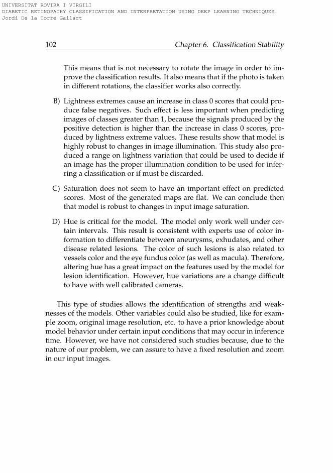
102 Chapter 6. Classification Stability
This means that is not necessary to rotate the image in order to im-prove the classification results. It also means that if the photo is takenin different rotations, the classifier works also correctly.
B) Lightness extremes cause an increase in class 0 scores that could pro-duce false negatives. Such effect is less important when predictingimages of classes greater than 1, because the signals produced by thepositive detection is higher than the increase in class 0 scores, pro-duced by lightness extreme values. These results show that model ishighly robust to changes in image illumination. This study also pro-duced a range on lightness variation that could be used to decide ifan image has the proper illumination condition to be used for infer-ring a classification or if must be discarded.
C) Saturation does not seem to have an important effect on predictedscores. Most of the generated maps are flat. We can conclude thenthat model is robust to changes in input image saturation.
D) Hue is critical for the model. The model only work well under cer-tain intervals. This result is consistent with experts use of color in-formation to differentiate between aneurysms, exhudates, and otherdisease related lesions. The color of such lesions is also related tovessels color and the eye fundus color (as well as macula). Therefore,altering hue has a great impact on the features used by the model forlesion identification. However, hue variations are a change difficultto have with well calibrated cameras.
This type of studies allows the identification of strengths and weak-nesses of the models. Other variables could also be studied, like for exam-ple zoom, original image resolution, etc. to have a prior knowledge aboutmodel behavior under certain input conditions that may occur in inferencetime. However, we have not considered such studies because, due to thenature of our problem, we can assure to have a fixed resolution and zoomin our input images.
UNIVERSITAT ROVIRA I VIRGILI DIABETIC RETINOPATHY CLASSIFICATION AND INTERPRETATION USING DEEP LEARNING TECHNIQUES Jordi De la Torre Gallart
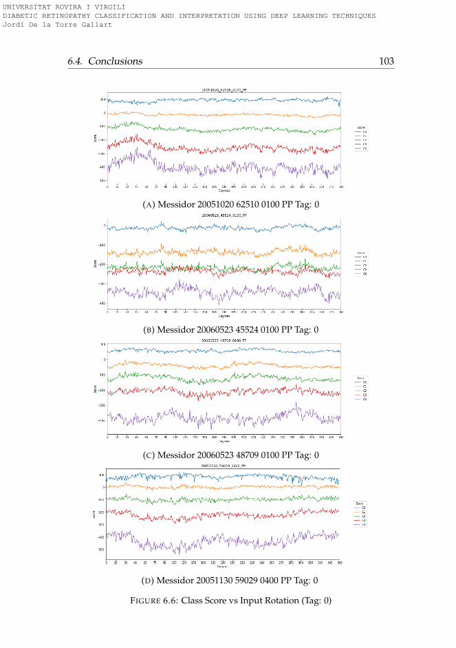
6.4. Conclusions 103
(A) Messidor 20051020 62510 0100 PP Tag: 0
(B) Messidor 20060523 45524 0100 PP Tag: 0
(C) Messidor 20060523 48709 0100 PP Tag: 0
(D) Messidor 20051130 59029 0400 PP Tag: 0
FIGURE 6.6: Class Score vs Input Rotation (Tag: 0)
UNIVERSITAT ROVIRA I VIRGILI DIABETIC RETINOPATHY CLASSIFICATION AND INTERPRETATION USING DEEP LEARNING TECHNIQUES Jordi De la Torre Gallart
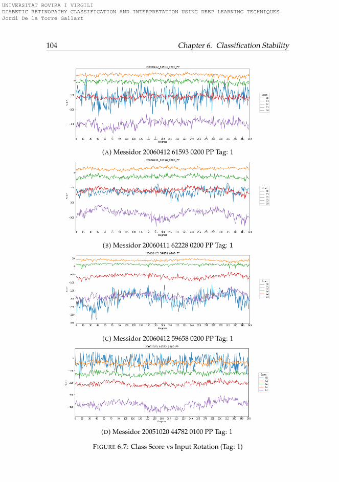
104 Chapter 6. Classification Stability
(A) Messidor 20060412 61593 0200 PP Tag: 1
(B) Messidor 20060411 62228 0200 PP Tag: 1
(C) Messidor 20060412 59658 0200 PP Tag: 1
(D) Messidor 20051020 44782 0100 PP Tag: 1
FIGURE 6.7: Class Score vs Input Rotation (Tag: 1)
UNIVERSITAT ROVIRA I VIRGILI DIABETIC RETINOPATHY CLASSIFICATION AND INTERPRETATION USING DEEP LEARNING TECHNIQUES Jordi De la Torre Gallart
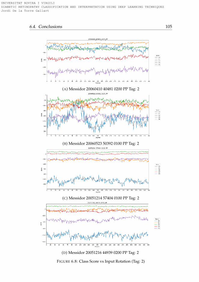
6.4. Conclusions 105
(A) Messidor 20060410 40481 0200 PP Tag: 2
(B) Messidor 20060523 50392 0100 PP Tag: 2
(C) Messidor 20051214 57404 0100 PP Tag: 2
(D) Messidor 20051216 44939 0200 PP Tag: 2
FIGURE 6.8: Class Score vs Input Rotation (Tag: 2)
UNIVERSITAT ROVIRA I VIRGILI DIABETIC RETINOPATHY CLASSIFICATION AND INTERPRETATION USING DEEP LEARNING TECHNIQUES Jordi De la Torre Gallart
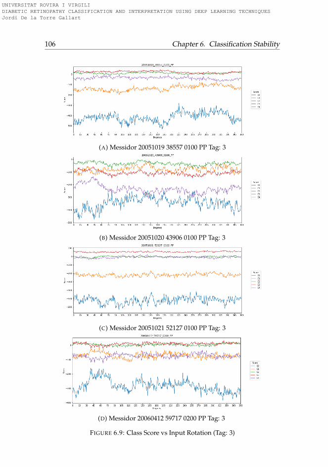
106 Chapter 6. Classification Stability
(A) Messidor 20051019 38557 0100 PP Tag: 3
(B) Messidor 20051020 43906 0100 PP Tag: 3
(C) Messidor 20051021 52127 0100 PP Tag: 3
(D) Messidor 20060412 59717 0200 PP Tag: 3
FIGURE 6.9: Class Score vs Input Rotation (Tag: 3)
UNIVERSITAT ROVIRA I VIRGILI DIABETIC RETINOPATHY CLASSIFICATION AND INTERPRETATION USING DEEP LEARNING TECHNIQUES Jordi De la Torre Gallart
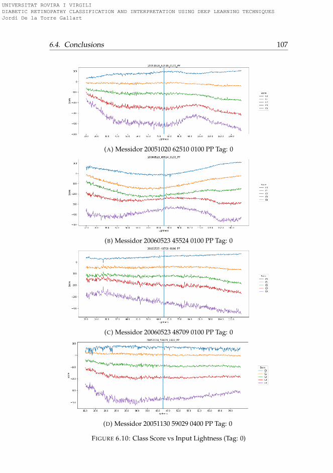
6.4. Conclusions 107
(A) Messidor 20051020 62510 0100 PP Tag: 0
(B) Messidor 20060523 45524 0100 PP Tag: 0
(C) Messidor 20060523 48709 0100 PP Tag: 0
(D) Messidor 20051130 59029 0400 PP Tag: 0
FIGURE 6.10: Class Score vs Input Lightness (Tag: 0)
UNIVERSITAT ROVIRA I VIRGILI DIABETIC RETINOPATHY CLASSIFICATION AND INTERPRETATION USING DEEP LEARNING TECHNIQUES Jordi De la Torre Gallart
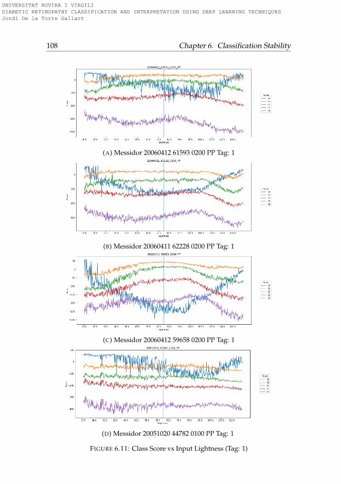
108 Chapter 6. Classification Stability
(A) Messidor 20060412 61593 0200 PP Tag: 1
(B) Messidor 20060411 62228 0200 PP Tag: 1
(C) Messidor 20060412 59658 0200 PP Tag: 1
(D) Messidor 20051020 44782 0100 PP Tag: 1
FIGURE 6.11: Class Score vs Input Lightness (Tag: 1)
UNIVERSITAT ROVIRA I VIRGILI DIABETIC RETINOPATHY CLASSIFICATION AND INTERPRETATION USING DEEP LEARNING TECHNIQUES Jordi De la Torre Gallart
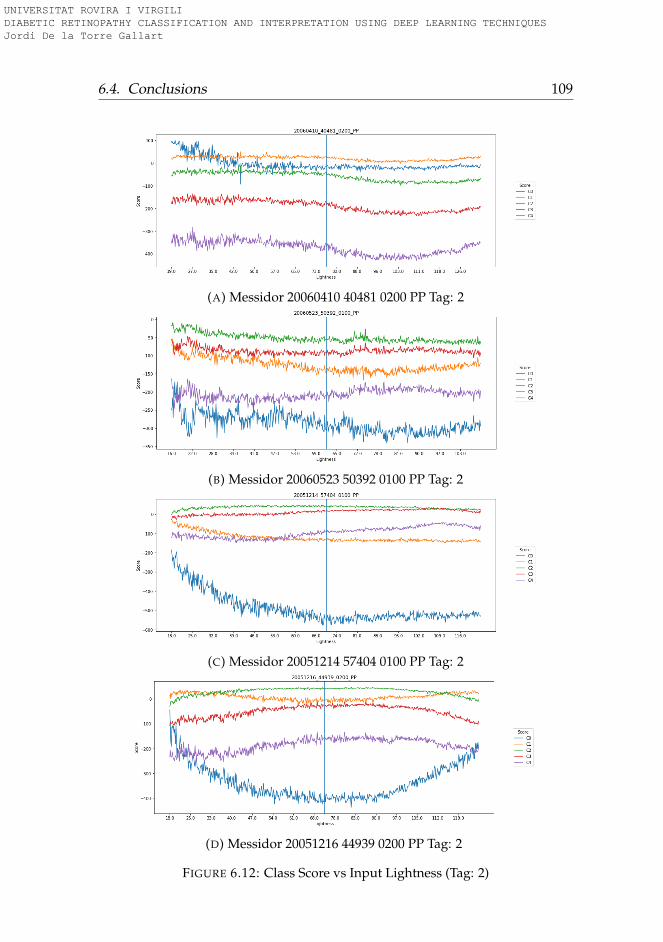
6.4. Conclusions 109
(A) Messidor 20060410 40481 0200 PP Tag: 2
(B) Messidor 20060523 50392 0100 PP Tag: 2
(C) Messidor 20051214 57404 0100 PP Tag: 2
(D) Messidor 20051216 44939 0200 PP Tag: 2
FIGURE 6.12: Class Score vs Input Lightness (Tag: 2)
UNIVERSITAT ROVIRA I VIRGILI DIABETIC RETINOPATHY CLASSIFICATION AND INTERPRETATION USING DEEP LEARNING TECHNIQUES Jordi De la Torre Gallart
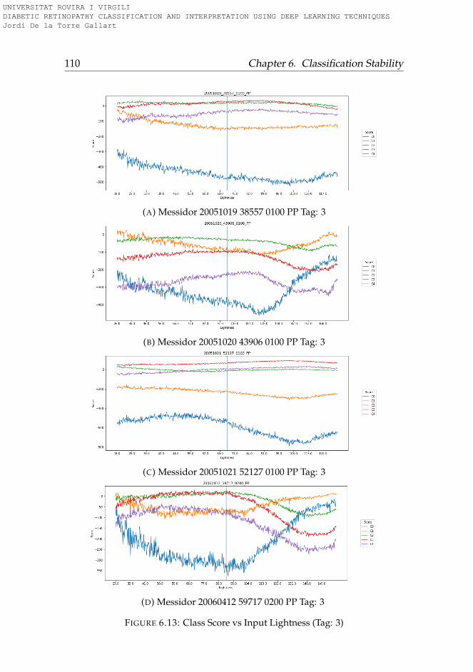
110 Chapter 6. Classification Stability
(A) Messidor 20051019 38557 0100 PP Tag: 3
(B) Messidor 20051020 43906 0100 PP Tag: 3
(C) Messidor 20051021 52127 0100 PP Tag: 3
(D) Messidor 20060412 59717 0200 PP Tag: 3
FIGURE 6.13: Class Score vs Input Lightness (Tag: 3)
UNIVERSITAT ROVIRA I VIRGILI DIABETIC RETINOPATHY CLASSIFICATION AND INTERPRETATION USING DEEP LEARNING TECHNIQUES Jordi De la Torre Gallart
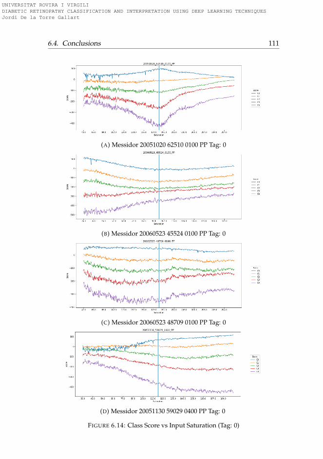
6.4. Conclusions 111
(A) Messidor 20051020 62510 0100 PP Tag: 0
(B) Messidor 20060523 45524 0100 PP Tag: 0
(C) Messidor 20060523 48709 0100 PP Tag: 0
(D) Messidor 20051130 59029 0400 PP Tag: 0
FIGURE 6.14: Class Score vs Input Saturation (Tag: 0)
UNIVERSITAT ROVIRA I VIRGILI DIABETIC RETINOPATHY CLASSIFICATION AND INTERPRETATION USING DEEP LEARNING TECHNIQUES Jordi De la Torre Gallart
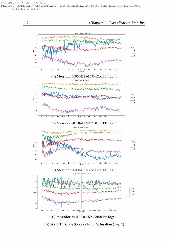
112 Chapter 6. Classification Stability
(A) Messidor 20060412 61593 0200 PP Tag: 1
(B) Messidor 20060411 62228 0200 PP Tag: 1
(C) Messidor 20060412 59658 0200 PP Tag: 1
(D) Messidor 20051020 44782 0100 PP Tag: 1
FIGURE 6.15: Class Score vs Input Saturation (Tag: 1)
UNIVERSITAT ROVIRA I VIRGILI DIABETIC RETINOPATHY CLASSIFICATION AND INTERPRETATION USING DEEP LEARNING TECHNIQUES Jordi De la Torre Gallart
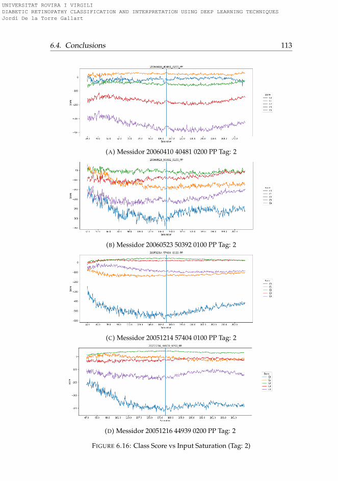
6.4. Conclusions 113
(A) Messidor 20060410 40481 0200 PP Tag: 2
(B) Messidor 20060523 50392 0100 PP Tag: 2
(C) Messidor 20051214 57404 0100 PP Tag: 2
(D) Messidor 20051216 44939 0200 PP Tag: 2
FIGURE 6.16: Class Score vs Input Saturation (Tag: 2)
UNIVERSITAT ROVIRA I VIRGILI DIABETIC RETINOPATHY CLASSIFICATION AND INTERPRETATION USING DEEP LEARNING TECHNIQUES Jordi De la Torre Gallart
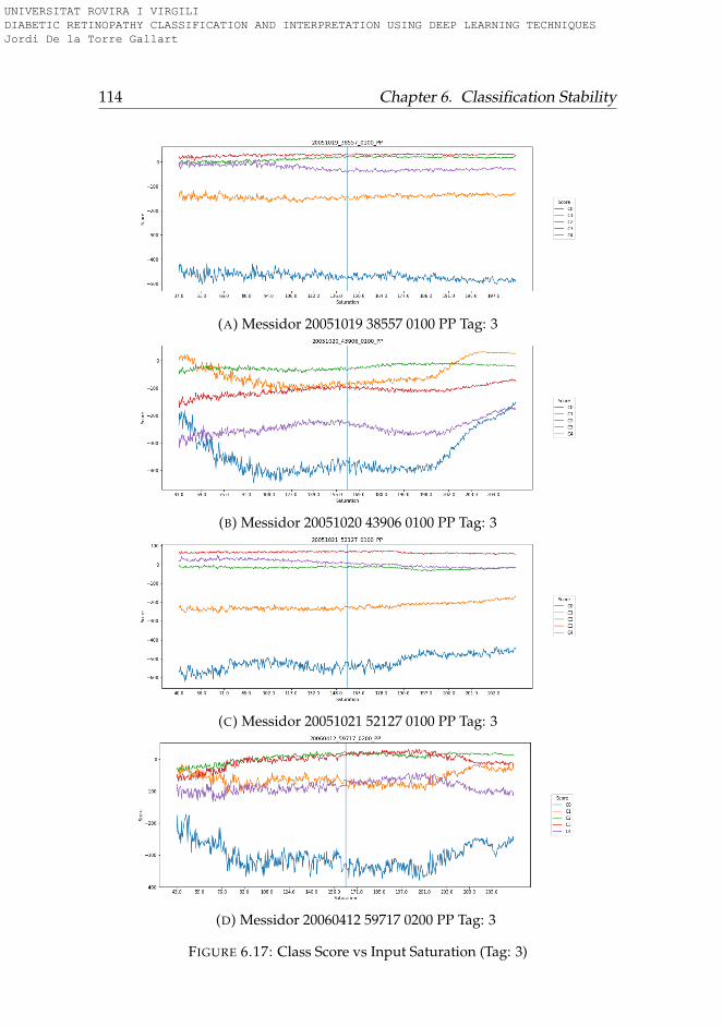
114 Chapter 6. Classification Stability
(A) Messidor 20051019 38557 0100 PP Tag: 3
(B) Messidor 20051020 43906 0100 PP Tag: 3
(C) Messidor 20051021 52127 0100 PP Tag: 3
(D) Messidor 20060412 59717 0200 PP Tag: 3
FIGURE 6.17: Class Score vs Input Saturation (Tag: 3)
UNIVERSITAT ROVIRA I VIRGILI DIABETIC RETINOPATHY CLASSIFICATION AND INTERPRETATION USING DEEP LEARNING TECHNIQUES Jordi De la Torre Gallart
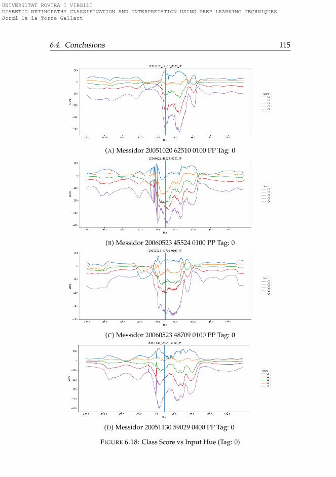
6.4. Conclusions 115
(A) Messidor 20051020 62510 0100 PP Tag: 0
(B) Messidor 20060523 45524 0100 PP Tag: 0
(C) Messidor 20060523 48709 0100 PP Tag: 0
(D) Messidor 20051130 59029 0400 PP Tag: 0
FIGURE 6.18: Class Score vs Input Hue (Tag: 0)
UNIVERSITAT ROVIRA I VIRGILI DIABETIC RETINOPATHY CLASSIFICATION AND INTERPRETATION USING DEEP LEARNING TECHNIQUES Jordi De la Torre Gallart
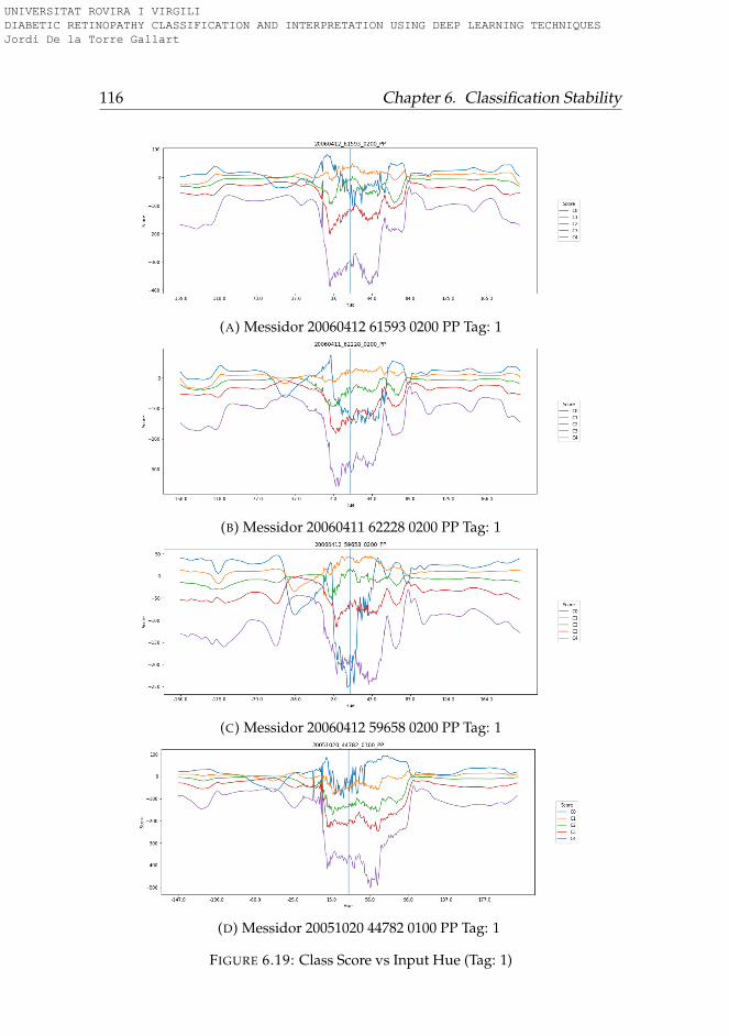
116 Chapter 6. Classification Stability
(A) Messidor 20060412 61593 0200 PP Tag: 1
(B) Messidor 20060411 62228 0200 PP Tag: 1
(C) Messidor 20060412 59658 0200 PP Tag: 1
(D) Messidor 20051020 44782 0100 PP Tag: 1
FIGURE 6.19: Class Score vs Input Hue (Tag: 1)
UNIVERSITAT ROVIRA I VIRGILI DIABETIC RETINOPATHY CLASSIFICATION AND INTERPRETATION USING DEEP LEARNING TECHNIQUES Jordi De la Torre Gallart
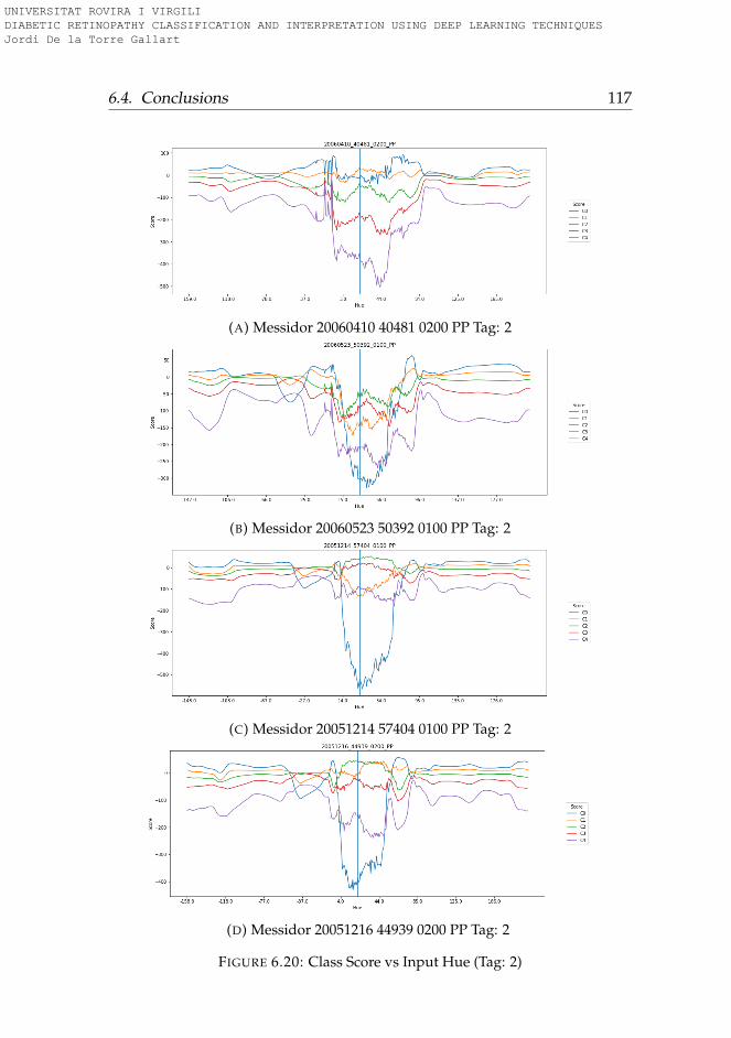
6.4. Conclusions 117
(A) Messidor 20060410 40481 0200 PP Tag: 2
(B) Messidor 20060523 50392 0100 PP Tag: 2
(C) Messidor 20051214 57404 0100 PP Tag: 2
(D) Messidor 20051216 44939 0200 PP Tag: 2
FIGURE 6.20: Class Score vs Input Hue (Tag: 2)
UNIVERSITAT ROVIRA I VIRGILI DIABETIC RETINOPATHY CLASSIFICATION AND INTERPRETATION USING DEEP LEARNING TECHNIQUES Jordi De la Torre Gallart
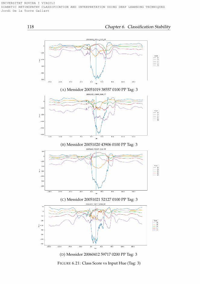
118 Chapter 6. Classification Stability
(A) Messidor 20051019 38557 0100 PP Tag: 3
(B) Messidor 20051020 43906 0100 PP Tag: 3
(C) Messidor 20051021 52127 0100 PP Tag: 3
(D) Messidor 20060412 59717 0200 PP Tag: 3
FIGURE 6.21: Class Score vs Input Hue (Tag: 3)
UNIVERSITAT ROVIRA I VIRGILI DIABETIC RETINOPATHY CLASSIFICATION AND INTERPRETATION USING DEEP LEARNING TECHNIQUES Jordi De la Torre Gallart
119
Part II
Interpretation
UNIVERSITAT ROVIRA I VIRGILI DIABETIC RETINOPATHY CLASSIFICATION AND INTERPRETATION USING DEEP LEARNING TECHNIQUES Jordi De la Torre Gallart

UNIVERSITAT ROVIRA I VIRGILI DIABETIC RETINOPATHY CLASSIFICATION AND INTERPRETATION USING DEEP LEARNING TECHNIQUES Jordi De la Torre Gallart
121
Chapter 7
Explanation Maps Generation
In this chapter we present work done regarding the interpretation goal ofthe thesis. In medical diagnosis tasks it is important not only the accuracyof predictions but also the reasons behind decisions. Self-explainable mod-els enable the physicians to contrast the information reported by the modelwith their own knowledge, increasing the probability of a good diagnostic,which may have a significant influence in patient’s treatment. The aim ofthis work is the elaboration of a general purpose interpretation algorithm,able to generate pixel maps that help in the interpretation of classificationresults reported by the model. With this model, it is possible to generateautomatically very precise lesion maps that are learn indirectly only fromgeneral classification information. The model encodes statistical regulari-ties present in data and the model presented in this chapter is able to visu-alize them. The system is organized using individual building blocks thatmake it easily transferable to be used with other architectures and in othercompletely different domains.
7.1 Introduction
Different attempts have been done for interpreting the results reported byneural networks. In (Zeiler and Fergus, 2014) a network propagation tech-nique is used for input-space feature visualization. After this work, (Bachet al., 2015) used a pixel-wise decomposition for classification problems.This decomposition could be done in two ways: considering the networkas a global function, disregarding its topology (functional approach) or us-ing the natural properties of the inherent function topology for applying a
UNIVERSITAT ROVIRA I VIRGILI DIABETIC RETINOPATHY CLASSIFICATION AND INTERPRETATION USING DEEP LEARNING TECHNIQUES Jordi De la Torre Gallart
122 Chapter 7. Explanation Maps Generation
message passing technique, propagating back into the pixel space the lastlayer output values. After this work, in (Montavon et al., 2017) they used aso-named Deep Taylor decomposition technique to replace the inherentlyintractable standard Taylor decomposition, using a multitude of simpleranalytically tractable Taylor decompositions.
In this chapter we follow an approach similar to pixel-wise decompo-sition taking into account the compositional nature of the topology, as in(Zeiler and Fergus, 2014) and (Bach et al., 2015). The concept of score inour chapter is similar to the concept of relevance used in the layer-wise rel-evance propagation method. The novelty of our approach comes from thefact that we assume that there are two factors that contribute to outputscore: one is the input-space contribution, while the other is a contributioncoming from the receptive fields of each layer. This last contribution de-pends solely on the parameters of each layer, thus being independent fromthe input-space. The second factor is not an attribute of the individual pix-els that has to be propagated back, but a contribution of the receptive field(RF) that represents the layer as an individual entity. Therefore, we onlypropagate back the score part that depends on the precedent input in eachlayer. In the proposed explanation model, we consider the constant partas a property of the RF of each layer. This approach allows us to do an ex-act propagation of the scores using a de-convolutional approach. Differingalso from (Zeiler and Fergus, 2014), our method allows the integration ofbatch normalization and of other typical neural network block constituentsinto the score propagation. A full set of score propagation blocks with themore typical DL functional constituents is derived in the chapter, in orderto facilitate the portability of this new explanatory method to other net-works and applications.
This interpretation model is tested in our application research area: Di-abetic Retinopathy for grading the level of disease. This model is able toreport the predicted class and also to score the importance of each pixel ofthe input image in the final classification decision. In such a way, it is pos-sible to determine which pixels in the input image are more important inthe final decision and facilitate the human experts an explanation to verifythe results reported by the model.
UNIVERSITAT ROVIRA I VIRGILI DIABETIC RETINOPATHY CLASSIFICATION AND INTERPRETATION USING DEEP LEARNING TECHNIQUES Jordi De la Torre Gallart
7.2. Related work 123
7.2 Related work
In last years, different approximations have been proposed to convert theinitial DL black box classifiers into interpretable classifiers. In the next sec-tions we introduce the most successful interpretation models existing to-day: sensitivity maps, layer-wise relevance propagation and Taylor decom-position models.
7.2.1 Sensitivity maps
Sensitivity maps (Simonyan, Vedaldi, and Zisserman, 2013) are pixel-spacematrices obtained from the calculation of ∂ f (I)
∂Ic,i,j∀c, i, j, where I is the input
image and f (I) is the DL function. These matrices are easy to calculate fordeep neural networks because they use the same backpropagation rulesthat are used during training, requiring only one more backpropagationstep for reaching the input-space. The problem with this approach is thatthere is no direct relationship between f (I) and ∇ f (I). The main concernof these models is that being the objective to explain f (x), ∂ f (I)
∂Ic,i,jis only
giving information about the local change of the function. For high non-linear functions, like deep neural networks, the local variation is pointingto the nearest local optimum, which should not necessarily be in the samedirection that the global minimum (Baehrens et al., 2010).
7.2.2 Layer-wise relevance propagation
In (Bach et al., 2015) the authors split the total score of a classification intoindividual relevance scores Rd that act as a positive or negative contributionsto the final result.
The method has the next general assumptions: the first one is the natureof the classification function, which has to be decomposable into severallayers of computation (like a deep neural network), the second is about thefact that the total relevance must be preserved from one layer to another,which means that the relevance of one layer is equal to the ones of all otherlayers (eq. 7.1) and, finally, the relevance of each node must be equal to thesum of all the incoming relevance messages of such node and also equal
UNIVERSITAT ROVIRA I VIRGILI DIABETIC RETINOPATHY CLASSIFICATION AND INTERPRETATION USING DEEP LEARNING TECHNIQUES Jordi De la Torre Gallart
124 Chapter 7. Explanation Maps Generation
to the sum of all the outgoing relevance messages from the same node (eq.7.2).
f (x) = ∑d∈l+1
R(l+1)d = ∑
d∈lR(l)
d = ... = ∑d
R(1)d (7.1)
where R(l)d is the relevance of node d in layer l.
R(l,l+1)i←k = R(l+1)
kaiωik
∑h ahωhk(7.2)
where R(l,l+1)i←k is the relevance message passing from node k located in
layer l + 1 to node i, located in layer l; ai is the activation of node i and ωijis the weight connecting node i and j.
7.2.3 Taylor-type decomposition
Another way for solving the interpretability problem is using the classifi-cation function gradient to calculate the next Taylor approximation (Bachet al., 2015):
f (I) ≈ f (I0) +∇(I0)[I − I0] = f (I0) +C
∑c=1
H
∑i=1
W
∑j=1
∂ f∂Ic,i,j
(Ic,i,j − I0c,i,j) (7.3)
Being I0 a free parameter that should be chosen in a way that f (I0) = 0in the case that f (I) is defined as a function that reports a value greaterthan one when belongs to the class, and lower than 0 otherwise. Definedin such a way, f (I) = 0 express the case of maximum uncertainty aboutthe image. Finding I0 allows us to express f (I) as:
f (I) ≈ ∇(I0)[I − I0] =C
∑c=1
H
∑i=1
W
∑j=1
∂ f∂Ic,i,j
(Ic,i,j − I0c,i,j) being f (I0) = 0
(7.4)
Equation 7.4 is per se an explanation of f (I) dependent only of the
UNIVERSITAT ROVIRA I VIRGILI DIABETIC RETINOPATHY CLASSIFICATION AND INTERPRETATION USING DEEP LEARNING TECHNIQUES Jordi De la Torre Gallart
7.3. Receptive field score distribution model 125
derivative function and of I0. The main concern of this approach is find-ing a valid root that is close to the analyzed image I using the Euclideannorm. In that way, we are approximating the function with a order 1 Taylorexpansion and the residuum is proportional to the Euclidean distance be-tween both points. Different ways for finding I0 have been proposed. Forexample, doing a unsupervised search of f (I) over the training set, lookingfor those images reporting f (I) near 0 and averaging them for finding I0.
7.2.4 Deep Taylor decomposition
Deep Taylor decomposition (Montavon et al., 2017) uses an approximationthat combines the layer-wise and Taylor type models. Taking advantageof the compositional nature of DL models, this approach assumes also thedecomposability of the relevance function, considering the existence forevery node of a partial relevance function Ri(ai) that depends on the acti-vation. It considers this function unknown and applies a Taylor decompo-sition through a root point. Summing up all the individual contributions,using the relevance conservation property defined in the previous mod-els, makes possible the propagation of intermediate relevance scores untileventually reach the input-space. Then, it generates a heat-map of the totalrelevance of the prediction in the input image.
7.3 Receptive field score distribution model
In this section we explain the new method proposed in this thesis for dis-tributing the output score into the previous layers in DL models (Torre,Valls, and Puig, 2017). We hypothesize that the output score of a partic-ular classification model is not only due to pixel score contributions butalso due to all the contributions of the receptive fields analyzed by the net-work. In next sections we will prove that, for all typical neural networktypes of layers, the output score can be expressed as the sum of layer’sconstants plus a value proportional to the layer’s input. Pixel-wise ex-planation model uses a similar approach for propagating backwards thescores, but with an important difference: pixel-wise (Bach et al., 2015) prop-agates back not only the input layer contribution, but also constants,suchas the bias, etc. Such a way of propagating backwards the scores breaks
UNIVERSITAT ROVIRA I VIRGILI DIABETIC RETINOPATHY CLASSIFICATION AND INTERPRETATION USING DEEP LEARNING TECHNIQUES Jordi De la Torre Gallart
126 Chapter 7. Explanation Maps Generation
the linear transformation. A way of maintaining the linear transformationis propagating backwards only the part that depends on the input, leav-ing the other part as a contribution of the layer (ie. of the receptive field).As the biases are not propagated, the normalization term used in pixel-wise method is not required anymore. Although neural network design isnon-linear, score back-propagation is linear over the activated nodes. Non-linear phase takes place in the forward pass, but the backward part onlytakes place over the activated nodes. In our formulation, we consider thescore entering into a node as the combination of two parts: one that can betransformed into a linear function dependent on the activated inputs andanother one that is constant for the considered node. Then, the final scoreis expressed as the sum of contributions of all nodes belonging to the stud-ied feature space (or pixel space) plus a constant score for the contributionof each node to every following layer. Such node constant scores dependon layer parameters and, in some way, on the output activations of the pre-vious layer. Thus, the propagated score depends solely on the individualactivation inputs of the layer. In such a way, we are able not only to finda unique way for mapping the score of every output in the input-space,but also and, most importantly, to find a linear relationship between out-put scores and image scores. This last property is due to the fact of usingexclusively linear transformations in all layers.
Formally, in this work, the following propositions are assumed:
Proposition 1. The score of every activation in the network is proportionalto the activation value:
Sl = λlal (7.5)
being Sl the tensor representative of all the scores of layer l, al the activa-tions tensor and λl another tensor establishing the required relationshipbetween Sl and al for l ∈ {1, ..., L}, being L the total number of layers.
Proposition 2. The score observed as output in one layer can be decom-posed into two parts: one dependent on the score of the previous layerSl−1 and another one Skl that is constant because it does not depend on theinput activations but only on the model parameters that are used in thatlayer:
Sl+1 = Sl + Skl (7.6)
UNIVERSITAT ROVIRA I VIRGILI DIABETIC RETINOPATHY CLASSIFICATION AND INTERPRETATION USING DEEP LEARNING TECHNIQUES Jordi De la Torre Gallart
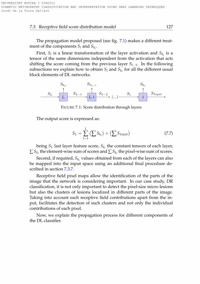
7.3. Receptive field score distribution model 127
The propagation model proposed (see fig. 7.1) makes a different treat-ment of the components Sl and Skl .
First, Sl is a linear transformation of the layer activation and Skl is atensor of the same dimensions independent from the activation that actsshifting the score coming from the previous layer Sl−1. In the followingsubsections we explain how to obtain Sl and Skl for all the different usualblock elements of DL networks.
L
SkL
L-1
SkL−1
(...) 1
Sk1
SL SL−1 SL−2 S1 SInput
FIGURE 7.1: Score distribution through layers
The output score is expressed as:
SL =L
∑l=1
(∑ Skl
)+(∑ SInput
)(7.7)
being SL last layer feature score, Skl the constant tensors of each layer,∑ Skl the element-wise sum of scores and ∑ Skl the pixel-wise sum of scores.
Second, if required, Skl values obtained from each of the layers can alsobe mapped into the input space using an additional final procedure de-scribed in section 7.3.7.
Receptive field pixel maps allow the identification of the parts of theimage that the network is considering important. In our case study, DRclassification, it is not only important to detect the pixel-size micro lesionsbut also the clusters of lesions localized in different parts of the image.Taking into account each receptive field contributions apart from the in-put, facilitates the detection of such clusters and not only the individualcontributions of each pixel.
Now, we explain the propagation process for different components ofthe DL classifier.
UNIVERSITAT ROVIRA I VIRGILI DIABETIC RETINOPATHY CLASSIFICATION AND INTERPRETATION USING DEEP LEARNING TECHNIQUES Jordi De la Torre Gallart
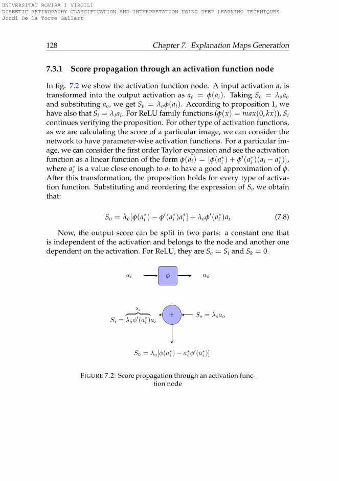
128 Chapter 7. Explanation Maps Generation
7.3.1 Score propagation through an activation function node
In fig. 7.2 we show the activation function node. A input activation ai istransformed into the output activation as ao = φ(ai). Taking So = λoaoand substituting ao, we get So = λoφ(ai). According to proposition 1, wehave also that Si = λiai. For ReLU family functions (φ(x) = max(0, kx)), Sicontinues verifying the proposition. For other type of activation functions,as we are calculating the score of a particular image, we can consider thenetwork to have parameter-wise activation functions. For a particular im-age, we can consider the first order Taylor expansion and see the activationfunction as a linear function of the form φ(ai) = [φ(a∗i ) + φ′(a∗i )(ai − a∗i )],where a∗i is a value close enough to ai to have a good approximation of φ.After this transformation, the proposition holds for every type of activa-tion function. Substituting and reordering the expression of So we obtainthat:
So = λo[φ(a∗i )− φ′(a∗i )a∗i ] + λoφ′(a∗i )ai (7.8)
Now, the output score can be split in two parts: a constant one thatis independent of the activation and belongs to the node and another onedependent on the activation. For ReLU, they are So = Si and Sk = 0.
ai φ ao
Si =
λi︷ ︸︸ ︷λoφ
′(a∗i )ai+ So = λoao
Sk = λo[φ(a∗i )− a∗iφ′(a∗i )]
FIGURE 7.2: Score propagation through an activation func-tion node
UNIVERSITAT ROVIRA I VIRGILI DIABETIC RETINOPATHY CLASSIFICATION AND INTERPRETATION USING DEEP LEARNING TECHNIQUES Jordi De la Torre Gallart
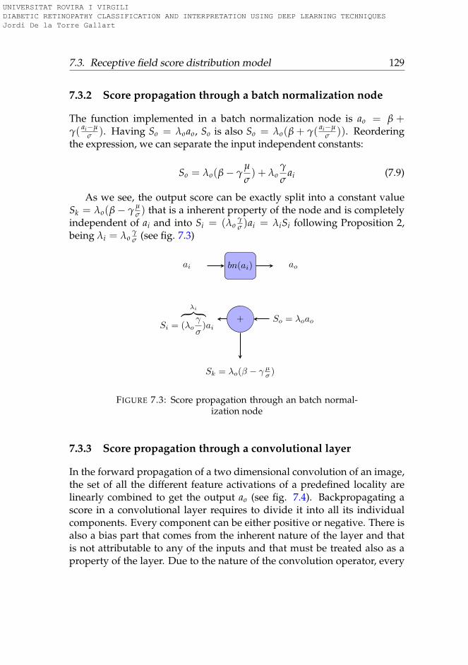
7.3. Receptive field score distribution model 129
7.3.2 Score propagation through a batch normalization node
The function implemented in a batch normalization node is ao = β +γ( ai−µ
σ ). Having So = λoao, So is also So = λo(β + γ( ai−µσ )). Reordering
the expression, we can separate the input independent constants:
So = λo(β− γµ
σ) + λo
γ
σai (7.9)
As we see, the output score can be exactly split into a constant valueSk = λo(β− γ
µσ ) that is a inherent property of the node and is completely
independent of ai and into Si = (λoγσ )ai = λiSi following Proposition 2,
being λi = λoγσ (see fig. 7.3)
ai bn(ai) ao
Si =
λi︷ ︸︸ ︷(λo
γ
σ)ai
+ So = λoao
Sk = λo(β − γ µσ )
FIGURE 7.3: Score propagation through an batch normal-ization node
7.3.3 Score propagation through a convolutional layer
In the forward propagation of a two dimensional convolution of an image,the set of all the different feature activations of a predefined locality arelinearly combined to get the output ao (see fig. 7.4). Backpropagating ascore in a convolutional layer requires to divide it into all its individualcomponents. Every component can be either positive or negative. There isalso a bias part that comes from the inherent nature of the layer and thatis not attributable to any of the inputs and that must be treated also as aproperty of the layer. Due to the nature of the convolution operator, every
UNIVERSITAT ROVIRA I VIRGILI DIABETIC RETINOPATHY CLASSIFICATION AND INTERPRETATION USING DEEP LEARNING TECHNIQUES Jordi De la Torre Gallart
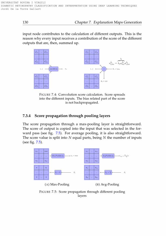
130 Chapter 7. Explanation Maps Generation
input node contributes to the calculation of different outputs. This is thereason why every input receives a contribution of the score of the differentoutputs that are, then, summed up.
af1i,11 ... af1i,1w
... ... ...
af1i,h1 ... af1i,hw
(...)
afNi,11 ... afNi,1w
... ... ...
afNi,h1 ... afNi,hw
conv2d(Ai) ao
sf1i,11 ... sf1i,1w
... ... ...
sf1i,h1 ... sf1i,hw
(...)
sfNi,11 ... sfNi,1w
... ... ...
sfNi,h1 ... sfNi,hw
+ So = λoao
Sk = λob
sfki,hw =
λi︷ ︸︸ ︷λoω
fkhwa
fki,hw
FIGURE 7.4: Convolution score calculation. Score spreadsinto the different inputs. The bias related part of the score
is not backpropagated.
7.3.4 Score propagation through pooling layers
The score propagation through a max-pooling layer is straightforward.The score of output is copied into the input that was selected in the for-ward pass (see fig. 7.5). For average pooling, it is also straightforward.The score value is split into N equal parts, being N the number of inputs(see fig. 7.5).
a11 ... max
... ... ...
ah1 ... ahw
MaxPool2d(Ai) ao = max
0 ... Si
... ... ...
0 ... 0
So = Si So
(A) Max-Pooling
a11 ... a1w
... ... ...
ah1 ... ahw
AvgPool2d(Ai) ao =∑
ij aij
N
S11 ... S1w
... ... ...
Sh1 ... Shw
Sij =So
N So
(B) Avg-Pooling
FIGURE 7.5: Score propagation through different poolinglayers
UNIVERSITAT ROVIRA I VIRGILI DIABETIC RETINOPATHY CLASSIFICATION AND INTERPRETATION USING DEEP LEARNING TECHNIQUES Jordi De la Torre Gallart
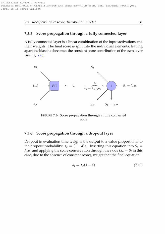
7.3. Receptive field score distribution model 131
7.3.5 Score propagation through a fully connected layer
A fully connected layer is a linear combination of the input activations andtheir weights. The final score is split into the individual elements, leavingapart the bias that becomes the constant score contribution of the own layer(see fig. 7.6).
a1
(...)
aN
FC ao
S1
Si =
λi︷︸︸︷λoωiai
SN
+ So = λoao
Sk = λob
FIGURE 7.6: Score propagation through a fully connectednode
7.3.6 Score propagation through a dropout layer
Dropout in evaluation time weights the output to a value proportional tothe dropout probability: ao = (1− d)ai. Inserting this equation into So =λoao and applying the score conservation through the node (So = Si in thiscase, due to the absence of constant score), we get that the final equation:
λi = λo(1− d) (7.10)
UNIVERSITAT ROVIRA I VIRGILI DIABETIC RETINOPATHY CLASSIFICATION AND INTERPRETATION USING DEEP LEARNING TECHNIQUES Jordi De la Torre Gallart
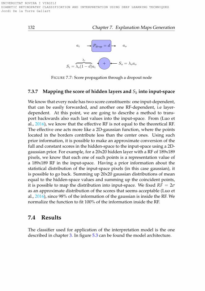
132 Chapter 7. Explanation Maps Generation
ai Pdrop = d ao
Si =
λi︷ ︸︸ ︷λo(1− d)ai
+ So = λoao
FIGURE 7.7: Score propagation through a dropout node
7.3.7 Mapping the score of hidden layers and Sk into input-space
We know that every node has two score constituents: one input-dependent,that can be easily forwarded, and another one RF-dependent, i.e layer-dependent. At this point, we are going to describe a method to trans-port backwards also such last values into the input-space. From (Luo etal., 2016), we know that the effective RF is not equal to the theoretical RF.The effective one acts more like a 2D-gaussian function, where the pointslocated in the borders contribute less than the center ones. Using suchprior information, it is possible to make an approximate conversion of thefull and constant scores in the hidden-space to the input-space using a 2D-gaussian prior. For example, for a 20x20 hidden layer with a RF of 189x189pixels, we know that each one of such points is a representation value ofa 189x189 RF in the input-space. Having a prior information about thestatistical distribution of the input-space pixels (in this case gaussian), itis possible to go back. Summing up 20x20 gaussian distributions of meanequal to the hidden-space values and summing up the coincident points,it is possible to map the distribution into input-space. We fixed RF = 2σas an approximate distribution of the scores that seems acceptable (Luo etal., 2016), since 98% of the information of the gaussian is inside the RF. Wenormalize the function to fit 100% of the information inside the RF.
7.4 Results
The classifier used for application of the interpretation model is the onedescribed in chapter 3. In figure 5.3 can be found the model architecture.
UNIVERSITAT ROVIRA I VIRGILI DIABETIC RETINOPATHY CLASSIFICATION AND INTERPRETATION USING DEEP LEARNING TECHNIQUES Jordi De la Torre Gallart
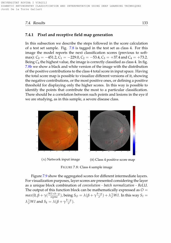
7.4. Results 133
7.4.1 Pixel and receptive field map generation
In this subsection we describe the steps followed in the score calculationof a test set sample. Fig. 7.8 is tagged in the test set as class 4. For thisimage the model reports the next classification scores (previous to soft-max): C0 = −451.2, C1 = −229.0, C2 = −53.4, C3 = +37.4 and C4 = +73.2.Being C4 the highest value, the image is correctly classified as class 4. In fig.7.8b we show a black and white version of the image with the distributionof the positive contributions to the class 4 total score in input space. Havingthe total score map is possible to visualize different versions of it, showingthe negative contributions, or the most positive ones, or defining a positivethreshold for displaying only the higher scores. In this way is possible toidentify the points that contribute the most to a particular classification.There should be a correlation between such points and lesions in the eye ifwe are studying, as in this sample, a severe disease class.
(A) Network input image (B) Class 4 positive score map
FIGURE 7.8: Class 4 sample image
Figure 7.9 show the aggregated scores for different intermediate layers.For visualization purposes, layer scores are presented considering the layeras a unique block combination of convolution - batch normalization - ReLU.The output of this function block can be mathematically expressed as O =
max(0, β + γ(WI+b−µsigma ), being SO = λ(β + γ
b−µσ ) + λ γ
σ WI. In this way SI =
λ γσ WI and Sk = λ(β + γ
b−µσ ).
UNIVERSITAT ROVIRA I VIRGILI DIABETIC RETINOPATHY CLASSIFICATION AND INTERPRETATION USING DEEP LEARNING TECHNIQUES Jordi De la Torre Gallart
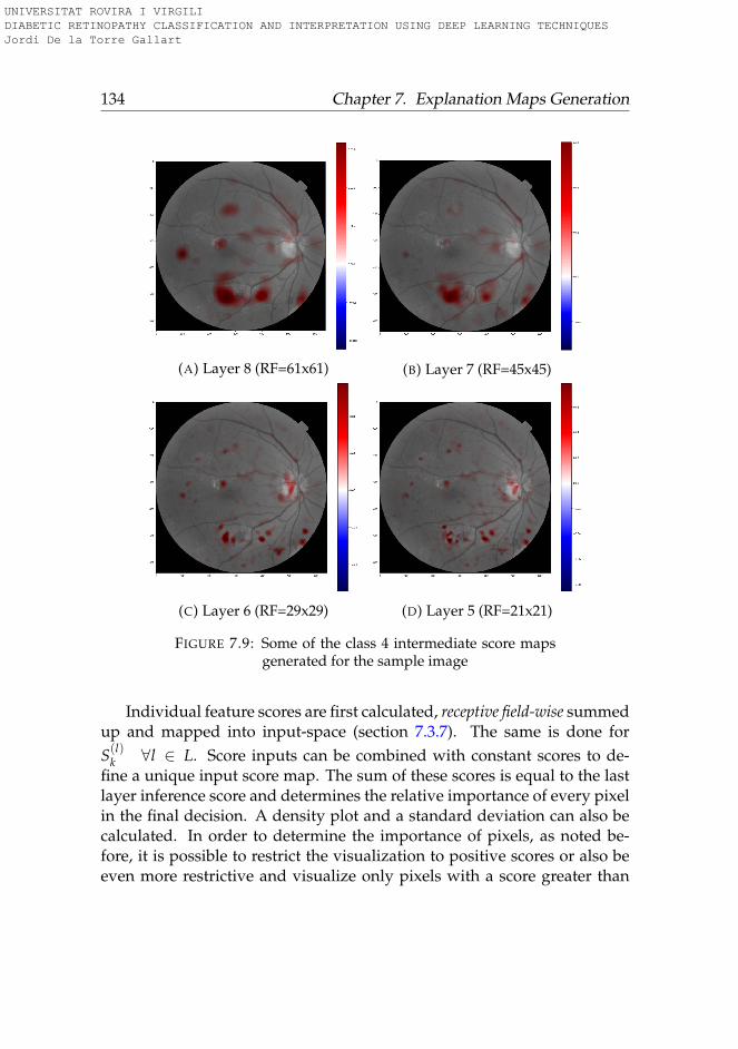
134 Chapter 7. Explanation Maps Generation
(A) Layer 8 (RF=61x61) (B) Layer 7 (RF=45x45)
(C) Layer 6 (RF=29x29) (D) Layer 5 (RF=21x21)
FIGURE 7.9: Some of the class 4 intermediate score mapsgenerated for the sample image
Individual feature scores are first calculated, receptive field-wise summedup and mapped into input-space (section 7.3.7). The same is done forS(l)
k ∀l ∈ L. Score inputs can be combined with constant scores to de-fine a unique input score map. The sum of these scores is equal to the lastlayer inference score and determines the relative importance of every pixelin the final decision. A density plot and a standard deviation can also becalculated. In order to determine the importance of pixels, as noted be-fore, it is possible to restrict the visualization to positive scores or also beeven more restrictive and visualize only pixels with a score greater than
UNIVERSITAT ROVIRA I VIRGILI DIABETIC RETINOPATHY CLASSIFICATION AND INTERPRETATION USING DEEP LEARNING TECHNIQUES Jordi De la Torre Gallart
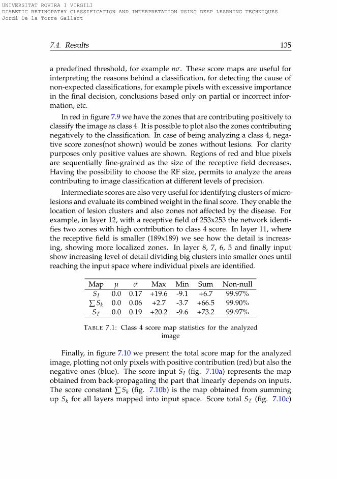
7.4. Results 135
a predefined threshold, for example nσ. These score maps are useful forinterpreting the reasons behind a classification, for detecting the cause ofnon-expected classifications, for example pixels with excessive importancein the final decision, conclusions based only on partial or incorrect infor-mation, etc.
In red in figure 7.9 we have the zones that are contributing positively toclassify the image as class 4. It is possible to plot also the zones contributingnegatively to the classification. In case of being analyzing a class 4, nega-tive score zones(not shown) would be zones without lesions. For claritypurposes only positive values are shown. Regions of red and blue pixelsare sequentially fine-grained as the size of the receptive field decreases.Having the possibility to choose the RF size, permits to analyze the areascontributing to image classification at different levels of precision.
Intermediate scores are also very useful for identifying clusters of micro-lesions and evaluate its combined weight in the final score. They enable thelocation of lesion clusters and also zones not affected by the disease. Forexample, in layer 12, with a receptive field of 253x253 the network identi-fies two zones with high contribution to class 4 score. In layer 11, wherethe receptive field is smaller (189x189) we see how the detail is increas-ing, showing more localized zones. In layer 8, 7, 6, 5 and finally inputshow increasing level of detail dividing big clusters into smaller ones untilreaching the input space where individual pixels are identified.
Map µ σ Max Min Sum Non-nullSI 0.0 0.17 +19.6 -9.1 +6.7 99.97%
∑ Sk 0.0 0.06 +2.7 -3.7 +66.5 99.90%ST 0.0 0.19 +20.2 -9.6 +73.2 99.97%
TABLE 7.1: Class 4 score map statistics for the analyzedimage
Finally, in figure 7.10 we present the total score map for the analyzedimage, plotting not only pixels with positive contribution (red) but also thenegative ones (blue). The score input SI (fig. 7.10a) represents the mapobtained from back-propagating the part that linearly depends on inputs.The score constant ∑ Sk (fig. 7.10b) is the map obtained from summingup Sk for all layers mapped into input space. Score total ST (fig. 7.10c)
UNIVERSITAT ROVIRA I VIRGILI DIABETIC RETINOPATHY CLASSIFICATION AND INTERPRETATION USING DEEP LEARNING TECHNIQUES Jordi De la Torre Gallart
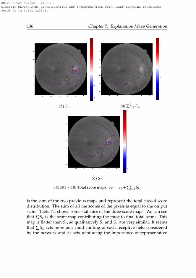
136 Chapter 7. Explanation Maps Generation
(A) SI (B) ∑Ll=1 Skl
(C) ST
FIGURE 7.10: Total score maps: ST = SI + ∑Ll=1 Skl
is the sum of the two previous maps and represent the total class 4 scoredistribution. The sum of all the scores of the pixels is equal to the outputscore. Table 7.1 shows some statistics of the three score maps. We can seethat ∑ Sk is the score map contributing the most to final total score. Thismap is flatter than SI , so qualitatively SI and ST are very similar. It seemsthat ∑ Sk acts more as a mild shifting of each receptive field consideredby the network and SI acts reinforcing the importance of representative
UNIVERSITAT ROVIRA I VIRGILI DIABETIC RETINOPATHY CLASSIFICATION AND INTERPRETATION USING DEEP LEARNING TECHNIQUES Jordi De la Torre Gallart
7.5. Conclusions 137
individual pixels.
7.5 Conclusions
In this chapter we proposed a method for generating, for every class, scoreimportance pixel maps, providing ophthalmologists the possibility of bothinference and interpretation. The reduced number of model parameters en-ables the use of these algorithms even in low resources devices, like mobilephones. The score generation is done back-propagating layer-wise onlythe score part that depends on the inputs and leaving the constant part asa contribution to the score of the considered layer. In this way, this methodis are able to generate scores in a unique and exact way.
Additionally, we have developed a technique, consisting on applyinga 2D-gaussian prior over the RFs, for mapping the constant hidden-spacescores to the input. With this technique we can generate a unique scoremap representative of the class, making possible to distribute the 100%score class information of the output layer.
We concluded also that for a good understanding of the causes behind aclassification, not only the pixel-space maps should be considered, but alsothe intermediate ones. The combination of the micro-information given bythe input space maps with the macro-information obtained from interme-diate scores is the key for understanding the results and to help the medicalpersonnel to improve the diagnosis processes.
UNIVERSITAT ROVIRA I VIRGILI DIABETIC RETINOPATHY CLASSIFICATION AND INTERPRETATION USING DEEP LEARNING TECHNIQUES Jordi De la Torre Gallart

UNIVERSITAT ROVIRA I VIRGILI DIABETIC RETINOPATHY CLASSIFICATION AND INTERPRETATION USING DEEP LEARNING TECHNIQUES Jordi De la Torre Gallart
139
Chapter 8
Feature Space Compression
The motivation of this work is the compression of information presentin diabetic retinopathy state-of-the-art models. Neural networks featurespaces are frequently high-dimensional spaces with high correlation val-ues between dimensions, ie. are low dimensional manifolds embedded inhigh dimensional spaces.
In this chapter a methodology for linear compression of the featurespace is presented, allowing the feature space compression from the orig-inal 64 dimensions to only 3 with a reduction of performance lower than2.5%.
8.1 Introduction
In this chapter we study a technique that allows the identification, sepa-ration and visualization in the input and hidden space of the independentcomponent (IC) responsible of a particular DR classification decision takenby a DL classifier given a certain eye fundus image. This is done by calcu-lating the minimum number of ICs that are able to encode the maximuminformation about the particular classification. Identifying such compo-nents, we reduce the redundancy of feature space and identify the com-ponents that share the minimum mutual information between each other.In that way, under the supposition that the feature extraction phase of thedeep learning model has been able to disentangle completely the featureinformation, we are able to separate the independent elements causing thedisease.
UNIVERSITAT ROVIRA I VIRGILI DIABETIC RETINOPATHY CLASSIFICATION AND INTERPRETATION USING DEEP LEARNING TECHNIQUES Jordi De la Torre Gallart
140 Chapter 8. Feature Space Compression
Independent Component Analysis (ICA) (Hyvärinen and Oja, 2000) isa statistical method for the separation of a multi-dimensional random sig-nal into a linear combination of components that are statistically as inde-pendent from each other as possible. The theoretical foundation of ICA isbased on the Central Limit Theorem, which establishes that the distribu-tion of the sum (average or linear combination) of N independent randomvariables approaches a gaussian as N → ∞. When ICA method is applied,it is assumed that such separation exist, ie. that is possible to express thesignal as a linear combination of independent components. Perfect inde-pendence between random variables is achieved when mutual informa-tion between them is zero. Mutual information can be expressed as theKullback-Leibler divergence between the joint distribution and the prod-uct of the distributions of each variable. Mutual information can be de-composed, under linear transforms, as the sum of two terms: one termexpressing the decorrelation of the components and one expressing theirnon-Gaussianity (Cardoso, 2003). ICA uses optimization to calculate itscomponents. Two types of optimization objectives can be used: minimizethe mutual information or maximize the non-gaussianess of each compo-nent.
We use the pixel-wise visualization method to identify in pixel spacesuch independent causes. We use the assessment of experts clinicians forinterpreting such ICs.
DL models are organized in layers, being the inputs of each one a com-bination of the outputs of previous ones. We design the output layer to be alinear combination of last layer feature space components. In this way weare forcing the model to disentangle the important features that, combinedin a linear way, allow the achievement of a maximum possible classifica-tion score. These components (or other obtained as a linear combination ofthem, like with ICA analysis), are easy to analyze due to the linear natureof its relationship with the classification scores.
8.2 ICA based interpretation procedure
In this chapter we go a step forward in the interpretation of score maps.Instead of generating directly the pixel maps associated with a particularclass, we try to identify and separate independent elements associated with
UNIVERSITAT ROVIRA I VIRGILI DIABETIC RETINOPATHY CLASSIFICATION AND INTERPRETATION USING DEEP LEARNING TECHNIQUES Jordi De la Torre Gallart
8.2. ICA based interpretation procedure 141
the disease. Our new contribution comes from the identification, separa-tion and visualization of the IC that explain a particular classification deci-sion. We hypothesize that in order to achieve high performance classifica-tion scores, the network has to encode the information required to make theclassification. Human experts base its decisions in the number and types oflesions present in the image. That’s why in some way, such information hasto be present in a disentangled form in last layer feature space, previous tothe output layer. Instead of directly visualizing the more important pixelsunder a classification decision, we split the information of such last featurelayer into independent features using a Independent Component Analysis(ICA). A posteriori we use a pixel-wise relevance propagation method tovisualize such independent component in input space. In this way, we can,not only generate importance pixel maps, but also differentiate betweenthe underlying independent causes of the disease.
First, we studied the last layer feature space, previous to the outputlayer linear combination in order to identify its properties and try to iso-late the independent elements that are causing a particular classification.For this purpose we used a principal component analysis (PCA) (Pear-son, 1901) to appraise the redundancy of this space and a ICA (Hyvärinenand Oja, 2000) using different number of components to identify the mini-mum of them required to achieve a classification score close enough to theachieved without such a dimensional reduction. ICA allows to find a lin-ear representation of non-Gaussian data so that the components are statis-tically independent, or as independent as possible. Such a representationseems to capture the essential structure of the data in many applications,including feature extraction (Hyvärinen and Oja, 2000). When the data isnot Gaussian, there are higher order statistics beyond variance that are nottaken into account by PCA. While PCA captures only uncorrelated compo-nents, these uncorrelated components are not necessarily independent forgeneral distributions. ICA minimizes the mutual information (or relativeKullback-Leibler divergence) of non-Gaussian data because two distribu-tions with zero mutual information are statistically independent (Comon,1994).
For finding the optimal number of IC, we apply ICA to the last layerfeature space training set vectors. Using different number of IC and com-paring the classification performance of the original model with the ob-tained using a linear combination of the reduced number of calculated
UNIVERSITAT ROVIRA I VIRGILI DIABETIC RETINOPATHY CLASSIFICATION AND INTERPRETATION USING DEEP LEARNING TECHNIQUES Jordi De la Torre Gallart
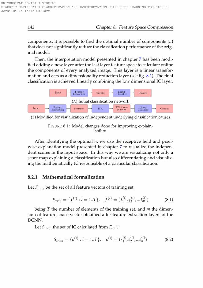
142 Chapter 8. Feature Space Compression
components, it is possible to find the optimal number of components (n)that does not significantly reduce the classification performance of the orig-inal model.
Then, the interpretation model presented in chapter 7 has been modi-fied adding a new layer after the last layer feature space to calculate onlinethe components of every analyzed image. This layer is a linear transfor-mation and acts as a dimensionality reduction layer (see fig. 8.1). The finalclassification is achieved linearly combining the low dimensional IC layer.
Input FeatureExtraction Features Linear
Classifier Classes
(A) Initial classification network
Input FeatureExtraction Features ICA
ICA Com-ponents
LinearClassifier Classes
(B) Modified for visualization of independent underlying classification causes
FIGURE 8.1: Model changes done for improving explain-ability
After identifying the optimal n, we use the receptive field and pixel-wise explanation model presented in chapter 7 to visualize the indepen-dent scores in the input space. In this way we are visualizing not only ascore map explaining a classification but also differentiating and visualiz-ing the mathematically IC responsible of a particular classification.
8.2.1 Mathematical formalization
Let Ftrain be the set of all feature vectors of training set:
Ftrain = { f (i) : i = 1..T}, f (i) = ( f (i)1 , f (i)2 , ... f (i)m ) (8.1)
being T the number of elements of the training set, and m the dimen-sion of feature space vector obtained after feature extraction layers of theDCNN.
Let Strain the set of IC calculated from Ftrain:
Strain = {s(i) : i = 1..T}, s(i) = (s(i)1 , s(i)2 , ...s(i)n ) (8.2)
UNIVERSITAT ROVIRA I VIRGILI DIABETIC RETINOPATHY CLASSIFICATION AND INTERPRETATION USING DEEP LEARNING TECHNIQUES Jordi De la Torre Gallart
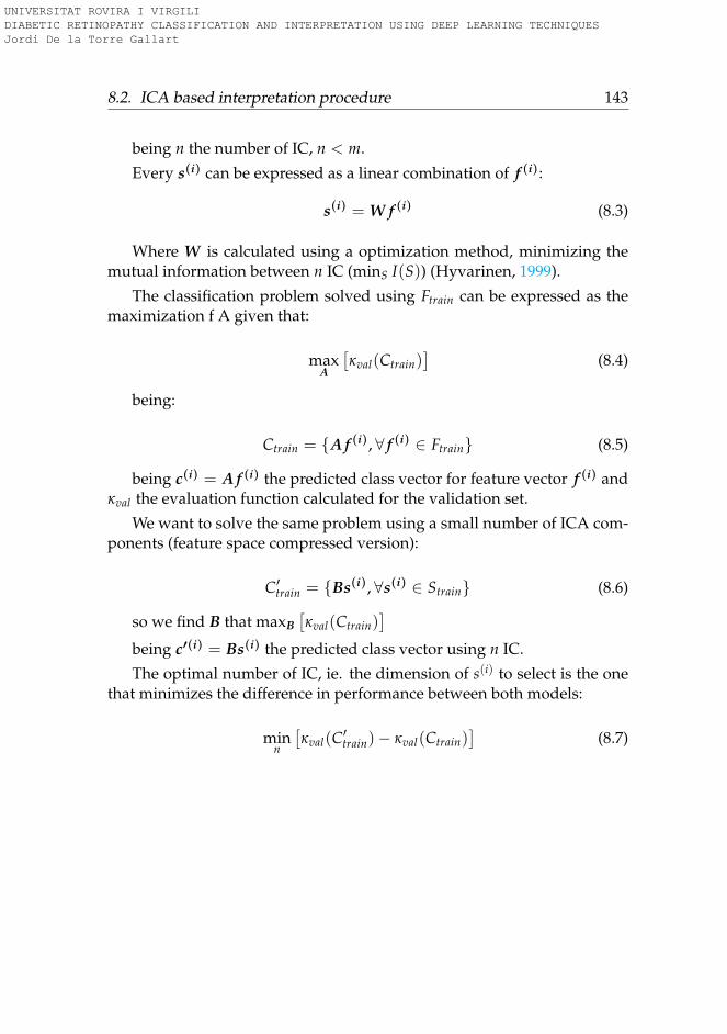
8.2. ICA based interpretation procedure 143
being n the number of IC, n < m.
Every s(i) can be expressed as a linear combination of f (i):
s(i) = W f (i) (8.3)
Where W is calculated using a optimization method, minimizing themutual information between n IC (minS I(S)) (Hyvarinen, 1999).
The classification problem solved using Ftrain can be expressed as themaximization f A given that:
maxA
[κval(Ctrain)
](8.4)
being:
Ctrain = {A f (i), ∀ f (i) ∈ Ftrain} (8.5)
being c(i) = A f (i) the predicted class vector for feature vector f (i) andκval the evaluation function calculated for the validation set.
We want to solve the same problem using a small number of ICA com-ponents (feature space compressed version):
C′train = {Bs(i), ∀s(i) ∈ Strain} (8.6)
so we find B that maxB[κval(Ctrain)
]
being c′(i) = Bs(i) the predicted class vector using n IC.
The optimal number of IC, ie. the dimension of s(i) to select is the onethat minimizes the difference in performance between both models:
minn
[κval(C′train)− κval(Ctrain)
](8.7)
UNIVERSITAT ROVIRA I VIRGILI DIABETIC RETINOPATHY CLASSIFICATION AND INTERPRETATION USING DEEP LEARNING TECHNIQUES Jordi De la Torre Gallart
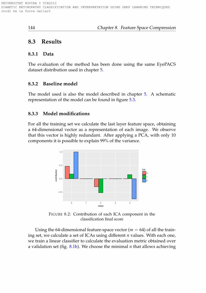
144 Chapter 8. Feature Space Compression
8.3 Results
8.3.1 Data
The evaluation of the method has been done using the same EyePACSdataset distribution used in chapter 5.
8.3.2 Baseline model
The model used is also the model described in chapter 5. A schematicrepresentation of the model can be found in figure 5.3.
8.3.3 Model modifications
For all the training set we calculate the last layer feature space, obtaininga 64-dimensional vector as a representation of each image. We observethat this vector is highly redundant. After applying a PCA, with only 10components it is possible to explain 99% of the variance.
−0.5
0.0
0.5
1.0
0 1 2 3 4
class
contr
ibution ica
0
1
2
FIGURE 8.2: Contribution of each ICA component in theclassification final score
Using the 64-dimensional feature-space vector (m = 64) of all the train-ing set, we calculate a set of ICAs using different n values. With each one,we train a linear classifier to calculate the evaluation metric obtained overa validation set (fig. 8.1b). We choose the minimal n that allows achieving
UNIVERSITAT ROVIRA I VIRGILI DIABETIC RETINOPATHY CLASSIFICATION AND INTERPRETATION USING DEEP LEARNING TECHNIQUES Jordi De la Torre Gallart
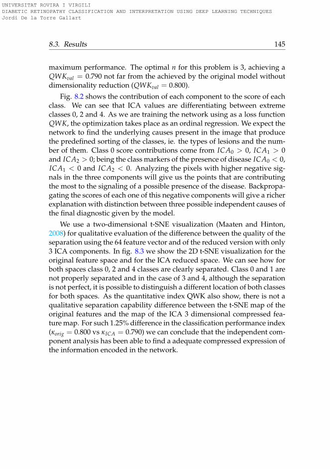
8.3. Results 145
maximum performance. The optimal n for this problem is 3, achieving aQWKval = 0.790 not far from the achieved by the original model withoutdimensionality reduction (QWKval = 0.800).
Fig. 8.2 shows the contribution of each component to the score of eachclass. We can see that ICA values are differentiating between extremeclasses 0, 2 and 4. As we are training the network using as a loss functionQWK, the optimization takes place as an ordinal regression. We expect thenetwork to find the underlying causes present in the image that producethe predefined sorting of the classes, ie. the types of lesions and the num-ber of them. Class 0 score contributions come from ICA0 > 0, ICA1 > 0and ICA2 > 0; being the class markers of the presence of disease ICA0 < 0,ICA1 < 0 and ICA2 < 0. Analyzing the pixels with higher negative sig-nals in the three components will give us the points that are contributingthe most to the signaling of a possible presence of the disease. Backpropa-gating the scores of each one of this negative components will give a richerexplanation with distinction between three possible independent causes ofthe final diagnostic given by the model.
We use a two-dimensional t-SNE visualization (Maaten and Hinton,2008) for qualitative evaluation of the difference between the quality of theseparation using the 64 feature vector and of the reduced version with only3 ICA components. In fig. 8.3 we show the 2D t-SNE visualization for theoriginal feature space and for the ICA reduced space. We can see how forboth spaces class 0, 2 and 4 classes are clearly separated. Class 0 and 1 arenot properly separated and in the case of 3 and 4, although the separationis not perfect, it is possible to distinguish a different location of both classesfor both spaces. As the quantitative index QWK also show, there is not aqualitative separation capability difference between the t-SNE map of theoriginal features and the map of the ICA 3 dimensional compressed fea-ture map. For such 1.25% difference in the classification performance index(κorig = 0.800 vs κICA = 0.790) we can conclude that the independent com-ponent analysis has been able to find a adequate compressed expression ofthe information encoded in the network.
UNIVERSITAT ROVIRA I VIRGILI DIABETIC RETINOPATHY CLASSIFICATION AND INTERPRETATION USING DEEP LEARNING TECHNIQUES Jordi De la Torre Gallart
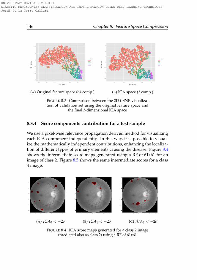
146 Chapter 8. Feature Space Compression
−60 −40 −20 0 20 40
−30
−20
−10
0
10
20
label01234
t− sne1
t−sn
e 2
(A) Original feature space (64 comp.)
−40 −20 0 20 40
−30
−20
−10
0
10
20
30
label01234
t− sne1
t−sn
e 2
(B) ICA space (3 comp.)
FIGURE 8.3: Comparison between the 2D t-SNE visualiza-tion of validation set using the original feature space and
the final 3-dimensional ICA space
8.3.4 Score components contribution for a test sample
We use a pixel-wise relevance propagation derived method for visualizingeach ICA component independently. In this way, it is possible to visual-ize the mathematically independent contributions, enhancing the localiza-tion of different types of primary elements causing the disease. Figure 8.4shows the intermediate score maps generated using a RF of 61x61 for animage of class 2. Figure 8.5 shows the same intermediate scores for a class4 image.
(A) ICA0 < −2σ (B) ICA1 < −2σ (C) ICA2 < −2σ
FIGURE 8.4: ICA score maps generated for a class 2 image(predicted also as class 2) using a RF of 61x61
UNIVERSITAT ROVIRA I VIRGILI DIABETIC RETINOPATHY CLASSIFICATION AND INTERPRETATION USING DEEP LEARNING TECHNIQUES Jordi De la Torre Gallart
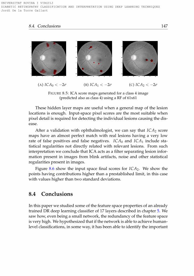
8.4. Conclusions 147
(A) ICA0 < −2σ (B) ICA1 < −2σ (C) ICA2 < −2σ
FIGURE 8.5: ICA score maps generated for a class 4 image(predicted also as class 4) using a RF of 61x61
These hidden layer maps are useful when a general map of the lesionlocations is enough. Input-space pixel scores are the most suitable whenpixel detail is required for detecting the individual lesions causing the dis-ease.
After a validation with ophthalmologist, we can say that ICA2 scoremaps have an almost perfect match with real lesions having a very lowrate of false positives and false negatives. ICA0 and ICA1 include sta-tistical regularities not directly related with relevant lesions. From suchinterpretation we conclude that ICA acts as a filter separating lesion infor-mation present in images from blink artifacts, noise and other statisticalregularities present in images.
Figure 8.6 show the input space final scores for ICA2. We show thepoints having contributions higher than a prestablished limit, in this casewith values higher than two standard deviations.
8.4 Conclusions
In this paper we studied some of the feature space properties of an alreadytrained DR deep learning classifier of 17 layers described in chapter 5. Wesaw how, even being a small network, the redundancy of the feature spaceis very high. We hypothesized that if the network is able to achieve human-level classifications, in some way, it has been able to identify the important
UNIVERSITAT ROVIRA I VIRGILI DIABETIC RETINOPATHY CLASSIFICATION AND INTERPRETATION USING DEEP LEARNING TECHNIQUES Jordi De la Torre Gallart
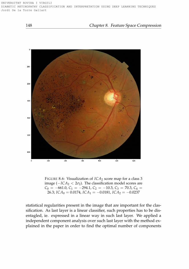
148 Chapter 8. Feature Space Compression
FIGURE 8.6: Visualization of ICA2 score map for a class 3image (−ICA2 < 2σ2). The classification model scores areC0 = −661.0, C1 = −294.1, C2 = −10.3, C3 = 70.3, C4 =
26.3; ICA0 = 0.0174, ICA1 = −0.0181, ICA2 = −0.0237
statistical regularities present in the image that are important for the clas-sification. As last layer is a linear classifier, such properties has to be dis-entagled, ie. expressed in a linear way in such last layer. We applied aindependent component analysis over such last layer with the method ex-plained in the paper in order to find the optimal number of components
UNIVERSITAT ROVIRA I VIRGILI DIABETIC RETINOPATHY CLASSIFICATION AND INTERPRETATION USING DEEP LEARNING TECHNIQUES Jordi De la Torre Gallart
8.4. Conclusions 149
that maximize the classification capabilities of such compressed versionof the features. We experimentally proved that reducing to only 3 com-ponents is possible to achieve almost 99% of the evaluation metric. Suchvalue experimentally prove that the ICA compression has been able to ex-tract all the important elements required for the classification. With suchelements, we applied a visualization technique for identifying the elementsin the image of each one of the components, using a pixel-wise derived vi-sualization technique. We are able to generate three maps for every imageeach one identifying independent statistical regularities important for theclassification.
Our method allows not only the classification of retinographies but alsothe identification and localization in the image of the independent signs ofthe disease. The presented ICA score model is of general applicability andcan be easily adapted for the usage in other image classification tasks.
UNIVERSITAT ROVIRA I VIRGILI DIABETIC RETINOPATHY CLASSIFICATION AND INTERPRETATION USING DEEP LEARNING TECHNIQUES Jordi De la Torre Gallart

UNIVERSITAT ROVIRA I VIRGILI DIABETIC RETINOPATHY CLASSIFICATION AND INTERPRETATION USING DEEP LEARNING TECHNIQUES Jordi De la Torre Gallart
151
Part III
Experimental Application andConclusions
UNIVERSITAT ROVIRA I VIRGILI DIABETIC RETINOPATHY CLASSIFICATION AND INTERPRETATION USING DEEP LEARNING TECHNIQUES Jordi De la Torre Gallart

UNIVERSITAT ROVIRA I VIRGILI DIABETIC RETINOPATHY CLASSIFICATION AND INTERPRETATION USING DEEP LEARNING TECHNIQUES Jordi De la Torre Gallart
153
Chapter 9
Inference using HUSJR data
In this chapter is presented a study done with the collaboration of a teamof ophthalmologists of Tarragona province with images collected during 8years at Hospital Universitari Sant Joan de Reus (HUSJR) in the framework ofthe Spanish project PI15/01150. The results show that the original modeltrained with EyePACS, after being fine-tuned for the prediction of classes,following the Messidor-2 standard, is able to predict with a high confidencethe ophthalmologists’ classifications.
9.1 Introduction
Machine Learning paradigm allow computer systems the ability to learnfrom data. These algorithms permit the identification of the most relevantfeatures and the way of combining them to maximize the performance ina particular classification or regression problem. Identifying such a set ofimportant features enables the generalization of prediction capabilities ofthe designed models.
After the training process we usually want to use the model for infer-ence over different data. New data can share a priori most of the prop-erties of data used in training, but also it may have distinctive proper-ties not present in the original data that could influence on the classifi-cation, ie. the probability distributions of both populations can be similarbut also have some differences. Therefore, before applying inference overthis new data, it is important to check for the existence of distinctive ele-ments affecting the classification/regression performance. If this happens,
UNIVERSITAT ROVIRA I VIRGILI DIABETIC RETINOPATHY CLASSIFICATION AND INTERPRETATION USING DEEP LEARNING TECHNIQUES Jordi De la Torre Gallart
154 Chapter 9. Inference using HUSJR data
we say that there is a dataset shift between both populations producing aco-variate shift in the model derived features used for prediction by themodel (Sugiyama, Lawrence, and Schwaighofer, 2017). Detecting or dis-carding such a co-variate shift is critical when using models from predic-tion in similar but different populations.
Exploratory Analysis using Graphical Methods are a very good wayof detecting the class separation quality. Feature-space domains are fre-quently highly correlated spaces that can be compressed into lower dimen-sional space representations. The shape of the internal representation ofthe data manifold determines the effectiveness of the dimensionality re-duction method. In cases where the manifold holds a linear representa-tion, methods like Principal Components Analysis (PCA) (Pearson, 1901),Multidimensional Scaling (MDS) (Kruskal, 1964) or Independent Compo-nents Analysis (ICA) (Hyvarinen, 1999) can be very effective. In caseswhere the manifold is non-linear or the points are to close to each other,non-linear techniques like Isometric Mapping (ISOMAP) (Tenenbaum, DeSilva, and Langford, 2000) or t-distributed Stochastic Neighboring Embed-ding (t-SNE) (Maaten and Hinton, 2008) are more effective.
For visualization purposes the objective is to find a method that is ableto separate diverging points and to cluster those with similar propertiesin a two-dimensional or three dimensional space. Even in cases where themanifold can be linearly compressed into a smaller representation, if thedimensions are more than three, it does not allow visualization, requiringthe usage of non-linear methods to reduce even more the dimensionalityto two or three dimensions.
t-SNE is a very effective visualization method that, with the proper se-lection of parameters, is able to separate effectively the different classespresent in the manifold. t-SNE uses an optimization algorithm to minimizethe Kullback-Leibler divergence (Kullback and Leibler, 1951) between twoprobability distributions, one in the original multidimensional space andanother one in the visualization space. Variables to optimize are the dis-tance between points in the visualization space.
Therefore, we will use t-SNE for the analysis of the dataset provided byHUSJR. We also have, in this case, the assistance of the ophtalmology teamof this hospital. So, we defined a four-step methodology for the testing ofthe classification model using their dataset. The description of this dataset
UNIVERSITAT ROVIRA I VIRGILI DIABETIC RETINOPATHY CLASSIFICATION AND INTERPRETATION USING DEEP LEARNING TECHNIQUES Jordi De la Torre Gallart
9.2. Methods 155
can be found in chapter 2.
9.2 Methods
In this section we present the method that is used for adapting the modeltrained with the EyePACS model to the HUSJR population.
The steps required for model adaptation can be summarized in: modelevaluation, standardization of categories, model and dataset adaptationsand final evaluation.
9.2.1 Original model evaluation
In this phase disease experts check the model predictions over the test setof the original model. The first thing that has to be checked is the compati-bility between class output definition in the original model with the classesdefined in the objective data set. If differences in class definition are identi-fied, they must be taken into account because it would require a retrainingof the model. This first step allows also the evaluation of the predictionsquality and to have a qualitative evaluation on original model test images.
9.2.2 Category standardization
The objective of this part is comparing if the categorization used in originalmodel is the same that is required in the target population. Sometimes,categories can be interpreted in slightly different ways if the definition ismore precisely established. This happens in medicine where subjectivityappears. If differences are detected, they require some adaptation either inthe target class or in the model class definitions.
9.2.3 Model and dataset adaptations
If evident discrepancies are detected, class re-definitions in original modeland target population should be applied, requiring either retraining inmodel or relabeling in target population. If model classes are redefined,the model must be retrained. If changes are mild, probably a last layer
UNIVERSITAT ROVIRA I VIRGILI DIABETIC RETINOPATHY CLASSIFICATION AND INTERPRETATION USING DEEP LEARNING TECHNIQUES Jordi De la Torre Gallart
156 Chapter 9. Inference using HUSJR data
classification retraining will suffice. If evaluation function results are notoptimal, deep changes are required, ie. a full network retraining.
9.2.4 Final evaluation
Finally, the modified dataset is tested with the classification model in orderto validate it. Having possible qualitative and quantitative results, the finalmodel can be used for inference in the new objective population.
9.3 Results
In this section we present the results of the four steps proposed for analyz-ing the HUSJR dataset.
9.3.1 Original model evaluation
The first important difference between model and the new population isthe categorization employed. Original model is designed for differentia-tion of 5 classes. HUSJR population distinguishes between only 4 classes.Expert analysis over images of the original data set indicate that, HUSJRclassification groups together class 3 and 4 of the original model.
Two tests are done in order to have a initial evaluation of the perfor-mance of the model:
Firstly, an evaluation of all images is done using the original DCNNmodel. Table 9.1 shows the results obtained of the classification. Cal-culated QWK index is 0.791 for 4 classes (grouping class 3 and 4). Thisvalue is about 1,6% lower than the achieved for the EyePACS test set, ie.QWK = 0.804 and a 5% lower than the achieved for Messidor-2 Dataset ofthe original model (QWK = 0.831).
Secondly, t-SNE is used for visualizing the feature-space vector repre-sentation of each image. Figure 9.1 shows a two-dimensional t-SNE visu-alization of the feature space. Each point representing an image and pointcolor representing the tagged class. We can see a gradation separationbetween classes very similar to the observed in original and in Messidordatasets.
UNIVERSITAT ROVIRA I VIRGILI DIABETIC RETINOPATHY CLASSIFICATION AND INTERPRETATION USING DEEP LEARNING TECHNIQUES Jordi De la Torre Gallart
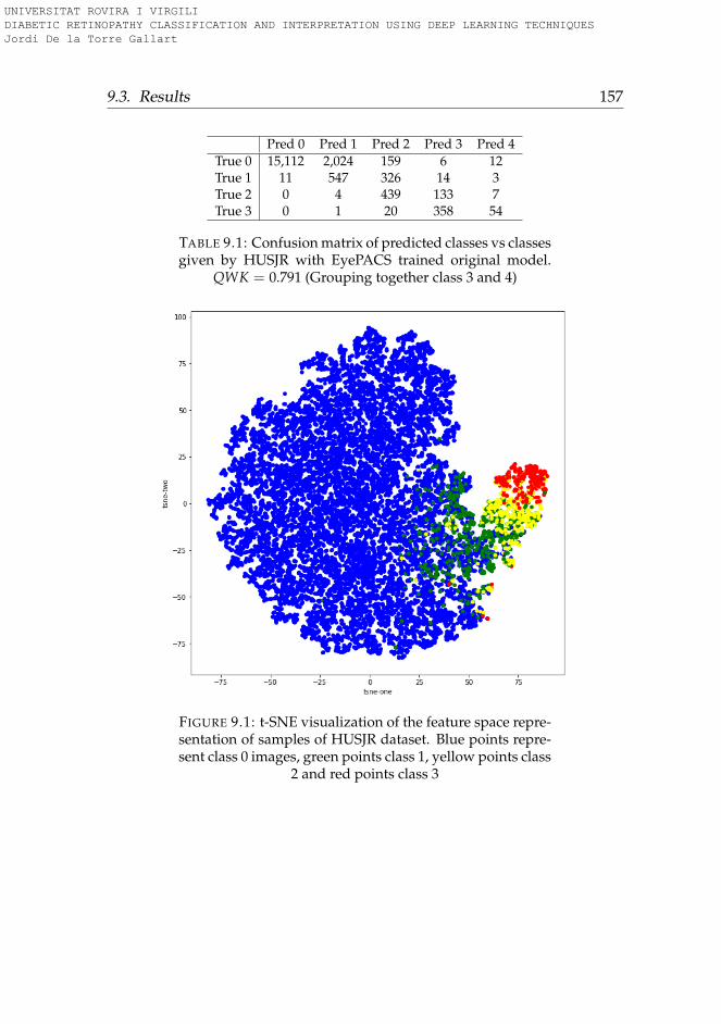
9.3. Results 157
Pred 0 Pred 1 Pred 2 Pred 3 Pred 4True 0 15,112 2,024 159 6 12True 1 11 547 326 14 3True 2 0 4 439 133 7True 3 0 1 20 358 54
TABLE 9.1: Confusion matrix of predicted classes vs classesgiven by HUSJR with EyePACS trained original model.
QWK = 0.791 (Grouping together class 3 and 4)
FIGURE 9.1: t-SNE visualization of the feature space repre-sentation of samples of HUSJR dataset. Blue points repre-sent class 0 images, green points class 1, yellow points class
2 and red points class 3
UNIVERSITAT ROVIRA I VIRGILI DIABETIC RETINOPATHY CLASSIFICATION AND INTERPRETATION USING DEEP LEARNING TECHNIQUES Jordi De la Torre Gallart
158 Chapter 9. Inference using HUSJR data
9.3.2 Category standardization
Due to the differences observed between the original classification and thenew one, HUSJR experts decide to use as a standard classification the de-fined one in Messidor-2 database (Decencière et al., 2014). In this catego-rization, only four classes are defined. HUSJR sample is reviewed to adaptthe original classification to the new defined standard.
9.3.3 Model adaptation
Original model is designed as a combination of a fully convolutional neuralnetwork that acts as a feature extractor. Features are linearly combined forclassification. Messidor-2 last layer feature vectors are calculated. A newlinear classifier is trained using these features for the prediction of newstandardized classes. The combination of original feature extractor withthe new last linear layer is used as a new prediction model for calculationof the new predicted classes of the HUSJR sample.
9.3.4 Results re-evaluation
The new confusion matrix obtained for HUSJR is presented in table 9.2.
Pred 0 Pred 1 Pred 2 Pred 3True 0 15,277 1,944 83 9True 1 5 595 284 17True 2 0 2 456 125True 3 0 1 6 426
TABLE 9.2: Confusion matrix of predicted classes vs orig-inal classes (HUSJR Dataset) with EyePACS trained origi-nal model plus a linear classifier retrained using Messidor
Dataset. QWK = 0.823
QWK inter-rater agreement evaluation index obtained (QWK = 0.823)is similar to the reached between ophthalmologist experts in disease detec-tion.
The indexes obtained for classification of the most severe cases of thedisease (considering positive class = 2,3 and negative class = 0,1) are:
UNIVERSITAT ROVIRA I VIRGILI DIABETIC RETINOPATHY CLASSIFICATION AND INTERPRETATION USING DEEP LEARNING TECHNIQUES Jordi De la Torre Gallart
9.4. Conclusions 159
• Sensitivity = 0.997
• Specificity = 0.978
• Positive predictive value (PPV) = 0.720
• Negative predictive value (NPV) = 0.9998
• False negative rate (FNR) = 0.003
• False positive rate (FPR) = 0.022
• False discovery rate (FDR) = 0.280
• False omission rate (FOR) = 0.0001
• Accuracy (ACC) = 0.979
• F1 Score = 0.836
• Matthews correlation coefficient (MCC) = 0.838
• Bookmaker Informedness (BM) = 0.975
• Markedness (MK) = 0.720
Sensitivity obtained is greater than 0.99 and Speci f icity near 0.98 forthe detection of the most severe cases of the disease. These and all theother indexes prove experimentally that the model is able to predict withhigh confidence the correct values of the disease for the new population ofstudy.
9.4 Conclusions
In this chapter, it is studied the applicability of our best model for the pre-diction of diabetic retinopathy, trained using the EyePACS dataset, for theprediction of diabetic retinopathy in HUSJR. A feature space visualizationhas been done in order to check its capacity for separating between classes.After checking that the separation was done properly, a first evaluation ofthe model predictability was done, obtaining good results, but with small
UNIVERSITAT ROVIRA I VIRGILI DIABETIC RETINOPATHY CLASSIFICATION AND INTERPRETATION USING DEEP LEARNING TECHNIQUES Jordi De la Torre Gallart
160 Chapter 9. Inference using HUSJR data
loss in performance. This loss was probably produced to the slight differ-ences in class definitions. After its standardization, the linear classifier ofthe model was retrained using Messidor-2 Dataset, using as a feature ex-tractor the original model. Performance of the new model was tested again,reaching values of inter-rater agreement similar to the obtained by expertophthalmologists. Classification indexes for the detection of the most se-vere cases of the disease are also presented, showing excellent performancealso over the new population. Modified model is ready to be used for in-ference over the new population. Medical team is extremely satisfied withthe results. Dr. Pere Romero, head of Ophthalmology Unit at HUSJR con-firms that the quality of the classification is good enough to be used in anear future.
UNIVERSITAT ROVIRA I VIRGILI DIABETIC RETINOPATHY CLASSIFICATION AND INTERPRETATION USING DEEP LEARNING TECHNIQUES Jordi De la Torre Gallart
161
Chapter 10
Conclusions
10.1 Summary of contributions
Medical diagnosis is heavily supported by Medical Imaging. The analy-sis of medical images requires highly specialized expertise that is providedby specialized doctors. The advent of advanced machine learning tech-niques, like deep learning, is facilitating the design of high performanceautomatic classifiers in a broad range of applications, also for medical di-agnosis. The purpose of this thesis is the exploration of new automaticdiagnostic methods for medical diagnosis, concretely for diabetic retinopa-thy disease grading. As stated before in this work, DR is one of the maincauses of blindness in the world. Early detection can reduce disease pro-gression and consequently also the incidence of blindness. The diagnosticof DR is done primarily by retina fundus image analysis, that is done byophthalmologists specifically trained for this purpose. Automatic diagnos-tic systems for DR can reduce dramatically not only the costs associated todiagnostic, but also the probability of developing blindness in the generalpopulation.
For this purpose we use supervised deep learning techniques. Givena class differentiation based on objective properties present in data, theseparameterized models are able to learn the statistical regularities that haveto be taken into account to separate the images. In this thesis, convolutionalneural networks are used, which are efficient neural networks designed forexploiting local high correlations present in images.
Machine learning methods in general and deep learning in particularare models that learn from data. Thus, a key factor for the success is having
UNIVERSITAT ROVIRA I VIRGILI DIABETIC RETINOPATHY CLASSIFICATION AND INTERPRETATION USING DEEP LEARNING TECHNIQUES Jordi De la Torre Gallart
162 Chapter 10. Conclusions
a statistically representative dataset of the population from which we wantto predict a concrete property, in this case, a disease class. For this purposeit is required to have a labeled dataset with enough samples (that are ofthe order of magnitude of thousands elements per class) in order to createmodels with good generalization. For this purpose, we use a public datasetof EyePACS. This dataset is described in chapter 2.
In chapter 3, we explore the first classification methods. In this casethe original images have different high resolution values. Ideally, it is in-teresting to use images with the highest resolution available, but mem-ory and computation time required make infeasible to use neural networkmodels in such conditions. Furthermore, neural networks architectures areparameterized models that require the usage of constant input size. Addi-tionally, lesions present in images, from which classification is inferred, canbe detected with lower resolutions. In this chapter, we explore the usageof different input sizes, data augmentation techniques and optimizationstrategies, that serve as a basis for selecting the best hyper-parameters. En-sembling techniques, averaging a set of predictions coming from the eval-uation of different rotated versions of the same input image, and bayesiananalysis, combining predictions of one patient eye with conditional prob-abilities of having the disease in the other, are also used for improving re-sults. From this preliminary work, a near human-level performance modelis obtained. Loss function used in this chapter for neural network param-eter optimization is the established standard for multi-class classification,ie. logarithmic loss.
As the evaluation function used for performance measure is quadraticweighted kappa, it is hypothesized that directly optimizing such functioncould generalize better. In chapter 4 it is presented a way to use quadraticweighted kappa as a loss function for optimization of neural networks.First order derivatives are developed, in order to facilitate its usage withgradient descent derived optimization methods. Different ordinal regres-sion use cases using quadratic weighted kappa as a main evaluation func-tion are studied, proving that in all of them, more than 5% increase in per-formance can be achieved optimizing directly QWK instead of logarithmicloss.
In chapter 5 the new hardware available enables the usage of higherinput resolutions and a faster computation time. This fact combined with
UNIVERSITAT ROVIRA I VIRGILI DIABETIC RETINOPATHY CLASSIFICATION AND INTERPRETATION USING DEEP LEARNING TECHNIQUES Jordi De la Torre Gallart
10.1. Summary of contributions 163
the usage of hyper-parameters selected in chapter 3 and with the designof the new loss function done in chapter 4 permits the design of modelswith ophthalmologist-level performance. In section 5.3.2 of this chapter,the most important hyper-parameters that have to be taken into account toachieve such results are summarized. This guidelines include parameterslike the input size, convolution operators recommended sizes, number offilters per layer, data augmentation strategies, etc.
In chapter 6, model robustness against changes in input images is alsostudied. Deep learning models are known to be very sensible to changesin input conditions. The objective of this chapter is the study of modelrobustness to typical changes in input conditions. The studied variablesare rotation, hue, saturation and lightness, experimentally proving that thedesigned model is robust to changes in lightness, saturation and rotationbut very sensible, as expected, to hue changes in input images. The huedependency seems to be due to the fact that network use color informationfor differentiating lesions from healthy tissue.
At this point, performance standards are achieved, but having the modelhigh statistical confidence, it shares with other deep learning models a ma-jor drawback, its lack of interpretability made it behave as a black box intu-ition machine. For improving medical applicability of such classifiers it isvery important not only to have a high confidence statistical classifier butalso to have a model that is able to provide an interpretation of the resultsto physicians.
With the idea of providing interpretation capabilities to our models,in chapter 7, a general purpose pixel-wise explanation model is designed.Such interpretation model backpropagates last layer classification scoresuntil reaching input space generating the so called pixel score maps, thatare maps with the distribution of the final score for each input pixel. Thepixels having higher scores are identified as the most important for a par-ticular classification. Such model propagates scores through the networkin two different ways: scores that depend on layer input are directly propa-gated to previous layer and constant scores of the layer, ie. related to biases,are transferred directly to the corresponding receptive field using a gaus-sian prior. Such interpretation model is designed in a modular manner,making it usable for any model architecture and in any application. In thisthesis, its validity for predicting lesions (that explain classifications for the
UNIVERSITAT ROVIRA I VIRGILI DIABETIC RETINOPATHY CLASSIFICATION AND INTERPRETATION USING DEEP LEARNING TECHNIQUES Jordi De la Torre Gallart
164 Chapter 10. Conclusions
diabetic retinopathy disease grading) is tested, achieving high correlationbetween predicted and real lesions.
In chapter 8, another way of improving interpretabilibity is explored,that is feature space data compression. Feature space deep learning mod-els tend to be high correlated, high dimensional spaces. In this chapter, amethod for compression of such space is proposed. In cases where classi-fication layer is designed as a linear feature combinations we assume thatthe model is able to disentangle the important features required for theclassification, making its dependency linear. For such models, a method isproposed for compressing the feature space based on Independent Com-ponent Analysis. A method for the selection of optimal number of com-ponents is proposed. The proposed method is of general applicability andits validity is tested using our diabetic retinopathy disease grading model.The original vector space of 64 dimensions is compressed to only three fea-tures, achieving 99% of performance of the original model without com-pression. Furthermore, such independent components can independentlyvisualized in the input space using the method designed in chapter 7.
Finally, in chapter 9 designed models are adapted to be used in a poten-tially different population coming from Hospital de Reus patients. Featurevisualization techniques were used in order to check that the class sepa-ration capabilities showed in the original model are compatible with thenew population, arriving to a positive conclusion. Compatibility of classdefinitions is also tested, detecting some discrepancies between the stan-dards defined in EyePACS and the HUSJR requirements. A retraining ofthe classification layer using Messidor-2 dataset was enough to achieveophtalmologist level accuracy in the new dataset.
After the work done in this thesis, we can conclude that designed mod-els can be used successfully as a high confidence diagnostic tool that canhelp to reduce costs in diagnostic and also to reduce the incidence of theDR disease in the general population.
UNIVERSITAT ROVIRA I VIRGILI DIABETIC RETINOPATHY CLASSIFICATION AND INTERPRETATION USING DEEP LEARNING TECHNIQUES Jordi De la Torre Gallart
10.2. Future research lines 165
10.2 Future research lines
After the work done in this PhD thesis and the knowledge we have gotfrom deep learning models as well as from diabetic retinopathy disease,some other study lines can be derived.
Future research lines can be focused on the next different directions,that we explain below:
1. Increase the number of classes to predict: One of the lines to explore isincreasing the number of properties to predict of the original model.Instead of only predicting diabetic retinopathy class, other classes canalso be included. Gradability class for example, can add informationabout image quality, ie. if its enough to be used as a proof of dis-ease. Macular Edema prediction can also be added, incrementing thedisease diagnostic information given by the automatic classifier. Fur-thermore, other diseases not directly related with diabetic retinopa-thy can also be detected, broadening the spectra of diagnostic. Wehypothesize that using the same network for diagnostic of differentdiseases can help to increase the network performance, due to the in-crease the number of images available and to the added diversity forthe detection of different diseases.
2. Transfer learning: Successful networks in challenging tasks like Ima-geNet, can be good candidates to perform well in specialized med-ical imaging tasks like ours. Transferring knowledge from trainednetworks to other completely different fields have been proven to bea good way to initialize networks and improving performance.
3. Unsupervised learning: Generative Adversarial Networks can also beexplored for generating new high quality samples from the originaldataset. Such sample generation models are able to generate poten-tially unlimited number of artificial training samples that could al-low, not only the training of more powerful models, but also the us-age of artificially generated images that do not belong to any particu-lar patient, ie. removing completely potential privacy legal concerns.
UNIVERSITAT ROVIRA I VIRGILI DIABETIC RETINOPATHY CLASSIFICATION AND INTERPRETATION USING DEEP LEARNING TECHNIQUES Jordi De la Torre Gallart
166 Chapter 10. Conclusions
4. Reinforcement Learning: Adding to the models the possibility of en-hancing its performance, designing online learning methods that al-low continuous learning of networks from the corrections done byophthalmologists on inference time. Hospital Universitari Sant Joande Reus wants to use the classification model developed in this the-sis in its daily work. This needs a previous process of integration ofcomputer systems as well as the permission of Catalan Health Careauthorities. If it is finally done, learning from online work could bevery interesting.
5. Use of Interpretation Model in other applications: The designed interpre-tation model is domain independent, therefore, it would be interest-ing the study of its application in other domains, ie. for interpretationof other medical imaging classification tasks like for example, radiol-ogy, ultrasound, or other related imaging applications.
6. Interpretation model for unsupervised image segmentation: Other inter-esting aspect to explore is its usage in the segmentation domain. Forthis particular area of expertise U-Net derived networks are workingvery well but it could be interesting to explore the usage of classifica-tion networks amplified with its interpretation model as a alternativeway of segmenting images without specifically annotating segmen-tation masks.
UNIVERSITAT ROVIRA I VIRGILI DIABETIC RETINOPATHY CLASSIFICATION AND INTERPRETATION USING DEEP LEARNING TECHNIQUES Jordi De la Torre Gallart
167
Bibliography
Aguiree, Florencia et al. (2013). “IDF diabetes atlas”. In:Aldington, SJ et al. (1995). “Methodology for retinal photography and as-
sessment of diabetic retinopathy: the EURODIAB IDDM complicationsstudy”. In: Diabetologia 38.4, pp. 437–444.
Bach, Sebastian et al. (2015). “On pixel-wise explanations for non-linearclassifier decisions by layer-wise relevance propagation”. In: PloS one10.7, e0130140.
Baehrens, David et al. (2010). “How to explain individual classification de-cisions”. In: Journal of Machine Learning Research 11.Jun, pp. 1803–1831.
Baldi, P. and P. Sadowski (2013). “Understanding Dropout”. In: Advances inNeural Information Processing Systems (NIPS). Ed. by C. J. C. Burges et al.Vol. 26, pp. 2814–2822.
Bengio, Yoshua (2009). “Learning deep architectures for AI”. In: Founda-tions and Trends in Machine Learning 2.1, pp. 1–127.
Bengio, Yoshua, Aaron Courville, and Pascal Vincent (Aug. 2013). “Repre-sentation Learning: A Review and New Perspectives”. In: IEEE Trans.Pattern Anal. Mach. Intell. 35.8, pp. 1798–1828. ISSN: 0162-8828.
Brain, Google (Nov. 2018). Diabetic Retinopathy grades (as well as DME andGradability) for the publicaly available MESSIDOR-2 fundus image database@ONLINE. URL: https://www.kaggle.com/google-brain/messidor2-dr-grades/home.
Bushberg, Jerrold T and John M Boone (2011). The essential physics of medicalimaging. Lippincott Williams & Wilkins.
Cardoso, Jean-François (2003). “Dependence, correlation and gaussianityin independent component analysis”. In: Journal of Machine Learning Re-search 4, pp. 1177–1203.
Chollet, François (2017). “Xception: Deep learning with depthwise separa-ble convolutions”. In: arXiv preprint, pp. 1610–02357.
UNIVERSITAT ROVIRA I VIRGILI DIABETIC RETINOPATHY CLASSIFICATION AND INTERPRETATION USING DEEP LEARNING TECHNIQUES Jordi De la Torre Gallart
168 Bibliography
Ciresan, Dan Claudiu et al. (2010). “Deep, Big, Simple Neural Nets forHandwritten Digit Recognition”. In: Neural Computation 22.12, pp. 3207–3220.
Clevert, Djork-Arné, Thomas Unterthiner, and Sepp Hochreiter (2015). “Fastand Accurate Deep Network Learning by Exponential Linear Units (ELUs)”.In: CoRR abs/1511.07289.
Cohen, Jacob (1960). “A coefficient of agreement for nominal scales”. In:Educational and psychological measurement 20.1, pp. 37–46.
— (1968). “Weighted kappa: Nominal scale agreement provision for scaleddisagreement or partial credit.” In: Psychological bulletin 70.4, p. 213.
Cohen, Nadav, Or Sharir, and Amnon Shashua (2016). “On the expressivepower of deep learning: A tensor analysis”. In: Conference on LearningTheory, pp. 698–728.
Comon, Pierre (1994). “Independent component analysis, a new concept?”In: Signal processing 36.3, pp. 287–314.
Dahl, George E., Tara N. Sainath, and Geoffrey E. Hinton (2013). “Improv-ing Deep Neural Networks for LVCSR using Rectified Linear Units andDropout”. In: IEEE International Conference on Acoustics, Speech and Sig-nal Processing (ICASSP), pp. 8609–8613.
Decencière, Etienne et al. (Aug. 2014). “Feedback on a publicly distributeddatabase: the Messidor database”. en. In: Image Analysis & Stereology33.3, pp. 231–234. ISSN: 1854-5165. DOI: 10.5566/ias.1155. URL: http://www.ias-iss.org/ojs/IAS/article/view/1155.
Deng, J. et al. (2009). “ImageNet: A Large-Scale Hierarchical Image Database”.In: CVPR09.
Dumoulin, Vincent and Francesco Visin (2016). “A guide to convolutionarithmetic for deep learning”. In: arXiv preprint arXiv:1603.07285.
Dundar, Aysegul, Jonghoon Jin, and Eugenio Culurciello (2015). “Convolu-tional Clustering for Unsupervised Learning”. In: CoRR abs/1511.06241.
Eldan, Ronen and Ohad Shamir (2016). “The power of depth for feedfor-ward neural networks”. In: Conference on Learning Theory, pp. 907–940.
Escorcia-Gutierrez, José et al. (2016). “Interactive Optic Disk Segmentationvia Discrete Convexity Shape Knowledge Using High-Order Function-als”. In: Artificial Intelligence Research and Development - Proceedings of the19th International Conference of the Catalan Association for Artificial Intelli-gence, Barcelona, Catalonia, Spain, October 19-21, 2016, pp. 39–44.
UNIVERSITAT ROVIRA I VIRGILI DIABETIC RETINOPATHY CLASSIFICATION AND INTERPRETATION USING DEEP LEARNING TECHNIQUES Jordi De la Torre Gallart
Bibliography 169
Esteva, Andre et al. (2017). “Dermatologist-level classification of skin can-cer with deep neural networks”. In: Nature 542.7639, p. 115.
EyePACS (Nov. 2018). EyePACS Dataset @ONLINE. URL: https://www.kaggle.com/c/diabetic-retinopathy-detection/data.
Fairchild, Mark D (2013). Color appearance models. John Wiley & Sons.Fleiss, Joseph L., Jacob Cohen, and B. S. Everitt (1969). “Large sample stan-
dard errors of kappa and weighted kappa”. In: Psychological Bulletin72(5), pp. 323–327.
Fong, Donald S et al. (2004). “Retinopathy in diabetes”. In: Diabetes care27.suppl 1, s84–s87.
Fukunaga, Keinosuke (2013). Introduction to statistical pattern recognition. El-sevier.
Glorot, Xavier and Yoshua Bengio (2010). “Understanding the difficulty oftraining deep feedforward neural networks”. In: Proceedings of the thir-teenth international conference on artificial intelligence and statistics, pp. 249–256.
Glorot, Xavier, Antoine Bordes, and Yoshua Bengio (2011). “Deep sparserectifier neural networks”. In: Proceedings of the fourteenth internationalconference on artificial intelligence and statistics, pp. 315–323.
Goodfellow, Ian, Yoshua Bengio, and Aaron Courville (2016). Deep Learn-ing. MIT Press.
Graham, Benjamin (2014). “Fractional Max-Pooling”. In: CoRR abs/1412.6071.Gulshan, V., L. Peng, and M. Coram (2016). “Development and validation
of a deep learning algorithm for detection of diabetic retinopathy inretinal fundus photographs”. In: Journal of the American Medical Associ-ation 316.22, pp. 2402–2410.
Günther, Klaus P and Yi Sun (1999). “Reliability of radiographic assess-ment in hip and knee osteoarthritis”. In: Osteoarthritis and Cartilage 7.2,pp. 239–246.
He, K. et al. (2015). “Delving Deep into Rectifiers: Surpassing Human-LevelPerformance on ImageNet Classification”. In: 2015 IEEE InternationalConference on Computer Vision (ICCV), pp. 1026–1034.
He, Kaiming et al. (2016). “Deep residual learning for image recognition”.In: Proceedings of the IEEE conference on computer vision and pattern recog-nition, pp. 770–778.
UNIVERSITAT ROVIRA I VIRGILI DIABETIC RETINOPATHY CLASSIFICATION AND INTERPRETATION USING DEEP LEARNING TECHNIQUES Jordi De la Torre Gallart
170 Bibliography
Hintz, Susan R et al. (2007). “Interobserver reliability and accuracy of cra-nial ultrasound scanning interpretation in premature infants”. In: TheJournal of pediatrics 150.6, pp. 592–596.
Howard, Andrew G et al. (2017). “Mobilenets: Efficient convolutional neu-ral networks for mobile vision applications”. In: arXiv preprint arXiv:1704.04861.
Hripcsak, George and Daniel F Heitjan (2002). “Measuring agreement inmedical informatics reliability studies”. In: Journal of biomedical infor-matics 35.2, pp. 99–110.
Huang, Gao et al. (2017). “Densely Connected Convolutional Networks.”In: CVPR. Vol. 1. 2, p. 3.
Hyvarinen, Aapo (1999). “Fast and robust fixed-point algorithms for inde-pendent component analysis”. In: IEEE transactions on Neural Networks10.3, pp. 626–634.
Hyvärinen, Aapo and Erkki Oja (2000). “Independent component analysis:algorithms and applications”. In: Neural networks 13.4-5, pp. 411–430.
Iandola, Forrest N et al. (2016). “Squeezenet: Alexnet-level accuracy with50x fewer parameters and< 0.5 mb model size”. In: arXiv preprint arXiv:1602.07360.
Ioffe, Sergey and Christian Szegedy (2015). “Batch Normalization: Accel-erating Deep Network Training by Reducing Internal Covariate Shift”.In: CoRR abs/1502.03167.
Kingma, Diederik P. and Jimmy Ba (2014). “Adam: A Method for StochasticOptimization”. In: CoRR abs/1412.6980.
Klein, Ronald et al. (2009). “The Wisconsin Epidemiologic Study of Dia-betic Retinopathy XXIII: the twenty-five-year incidence of macular edemain persons with type 1 diabetes”. In: Ophthalmology 116.3, pp. 497–503.
Krizhevsky, Alex, Ilya Sutskever, and Geoffrey E Hinton (2012a). “Ima-geNet Classification with Deep Convolutional Neural Networks”. In:Advances in Neural Information Processing Systems 25. Ed. by F. Pereiraet al. Curran Associates, Inc., pp. 1097–1105.
Krizhevsky, Alex, Ilya Sutskever, and Geoffrey E. Hinton (2012b). “Ima-geNet Classification with Deep Convolutional Neural Networks”. In:Advances in Neural Information Processing Systems 25. Ed. by F. Pereiraet al. Curran Associates, Inc., pp. 1097–1105.
Kruskal, Joseph B (1964). “Multidimensional scaling by optimizing good-ness of fit to a nonmetric hypothesis”. In: Psychometrika 29.1, pp. 1–27.
Kullback, Solomon and Richard A Leibler (1951). “On information and suf-ficiency”. In: The annals of mathematical statistics 22.1, pp. 79–86.
UNIVERSITAT ROVIRA I VIRGILI DIABETIC RETINOPATHY CLASSIFICATION AND INTERPRETATION USING DEEP LEARNING TECHNIQUES Jordi De la Torre Gallart
Bibliography 171
La Torre, Jordi de et al. (2018). “Identification and Visualization of the Un-derlying Independent Causes of the Diagnostic of Diabetic Retinopathymade by a Deep Learning Classifier”. In: CoRR abs/1809.08567. arXiv:1809.08567. URL: http://arxiv.org/abs/1809.08567.
Landis, J Richard and Gary G Koch (1977). “The measurement of observeragreement for categorical data”. In: biometrics, pp. 159–174.
LeCun, Y. et al. (1998). “Gradient-Based Learning Applied to DocumentRecognition”. In: Proceedings of the IEEE 86.11, pp. 2278–2324.
Lecun, Yann, Yoshua Bengio, and Geoffrey Hinton (May 2015). “Deep learn-ing”. In: Nature 521.7553, pp. 436–444. ISSN: 0028-0836.
LeCun, Yann et al. (1989). “Backpropagation applied to handwritten zipcode recognition”. In: Neural computation 1.4, pp. 541–551.
Liao, Zhibin and Gustavo Carneiro (2015). “Competitive Multi-scale Con-volution”. In: CoRR abs/1511.05635.
Luo, Wenjie et al. (2016). “Understanding the effective receptive field indeep convolutional neural networks”. In: Advances in Neural InformationProcessing Systems, pp. 4898–4906.
MA, Mazurowski et al. (2008). “Training neural network classifiers for med-ical decision making: The effects of imbalanced datasets on classifica-tion performance”. In: Neural Networks 21(2-3), pp. 427–436.
Maaten, Laurens van der and Geoffrey Hinton (2008). “Visualizing datausing t-SNE”. In: Journal of machine learning research 9.Nov, pp. 2579–2605.
Mehdiyev, Nijat et al. (2016). “Evaluating Forecasting Methods by Consid-ering Different Accuracy Measures”. In: Procedia Computer Science 95,pp. 264–271.
Montavon, Grégoire et al. (2017). “Explaining nonlinear classification deci-sions with deep taylor decomposition”. In: Pattern Recognition 65, pp. 211–222.
Murphy, Kevin P. (2012). Machine Learning: A Probabilistic Perspective. TheMIT Press. ISBN: 0262018020, 9780262018029.
Nair, Vinod and Geoffrey E Hinton (2010). “Rectified linear units improverestricted boltzmann machines”. In: Proceedings of the 27th internationalconference on machine learning (ICML-10), pp. 807–814.
Patra, S et al. (2009). “Interobserver agreement between primary gradersand an expert grader in the Bristol and Weston diabetic retinopathy
UNIVERSITAT ROVIRA I VIRGILI DIABETIC RETINOPATHY CLASSIFICATION AND INTERPRETATION USING DEEP LEARNING TECHNIQUES Jordi De la Torre Gallart
172 Bibliography
screening programme: a quality assurance audit”. In: Diabetic Medicine26.8, pp. 820–823.
Pearson, Karl (1901). “Principal components analysis”. In: The London, Ed-inburgh, and Dublin Philosophical Magazine and Journal of Science 6.2, p. 559.
Ramos, Juan (2003). Using TF-IDF to Determine Word Relevance in DocumentQueries. Tech. rep. Department of Computer Science, Rutgers Univer-sity, 23515 BPO Way, Piscataway, NJ, 08855e.
Romero-Aroca, Pedro et al. (2006). “Nonproliferative diabetic retinopathyand macular edema progression after phacoemulsification: prospectivestudy”. In: Journal of Cataract & Refractive Surgery 32.9, pp. 1438–1444.
Romero-Aroca, Pedro et al. (2018). “A Clinical Decision Support Systemfor Diabetic Retinopathy Screening: Creating a Clinical Support Appli-cation”. In: Telemedicine and e-Health.
Russakovsky, Olga et al. (2015). “ImageNet Large Scale Visual Recogni-tion Challenge”. In: International Journal of Computer Vision (IJCV) 115.3,pp. 211–252.
Saad, David (1998). “Online algorithms and stochastic approximations”.In: Online Learning 5.
Sammut, Claude and Geoffrey I Webb (2011). Encyclopedia of machine learn-ing. Springer Science & Business Media.
Sandler, Mark et al. (2018). “MobileNetV2: Inverted Residuals and LinearBottlenecks”. In: Proceedings of the IEEE Conference on Computer Visionand Pattern Recognition, pp. 4510–4520.
Schmidhuber, J. (2015). “Deep Learning in Neural Networks: An Overview”.In: Neural Networks 61, pp. 85–117.
SE, Moss et al. (1985). “Comparison Between Ophthalmoscopy and Fun-dus Photography in Determining Severity of Diabetic Retinopathy”. In:Ophthalmology 92(1), pp. 62–67.
Sermanet, Pierre et al. (2014). “Overfeat: Integrated recognition, localiza-tion and detection using convolutional networks”. In: International Con-ference on Learning Representations (ICLR2014), CBLS, April 2014.
Shaw, Jonathan E, Richard A Sicree, and Paul Z Zimmet (2010). “Globalestimates of the prevalence of diabetes for 2010 and 2030”. In: Diabetesresearch and clinical practice 87.1, pp. 4–14.
Sim, Julius and Chris C Wright (2005). “The kappa statistic in reliabilitystudies: use, interpretation, and sample size requirements”. In: Physicaltherapy 85.3, pp. 257–268.
UNIVERSITAT ROVIRA I VIRGILI DIABETIC RETINOPATHY CLASSIFICATION AND INTERPRETATION USING DEEP LEARNING TECHNIQUES Jordi De la Torre Gallart
Bibliography 173
Simonyan, Karen, Andrea Vedaldi, and Andrew Zisserman (2013). “DeepInside Convolutional Networks: Visualising Image Classification Mod-els and Saliency Maps”. In: CoRR abs/1312.6034. arXiv: 1312.6034.
Simonyan, Karen and Andrew Zisserman (2014). “Very Deep Convolu-tional Networks for Large-Scale Image Recognition”. In: CoRR abs/1409.1556.
— (2015). “Very Deep Convolutional Networks for Large-Scale Image Recog-nition”. In: International Conference on Learning Representations, ICLR 2015.
Sudha, L. R. and S. Thirupurasundari (2014). “Analysis and detection ofhaemorrhages and exhudates in retinal images”. In: International Journalof Scientific and Research Publications 4, pp. 1–5.
Sugiyama, Masashi, Neil D Lawrence, Anton Schwaighofer, et al. (2017).Dataset shift in machine learning. The MIT Press.
Szegedy, Christian et al. (2015). “Going Deeper with Convolutions”. In:Computer Vision and Pattern Recognition (CVPR).
Szegedy, Christian et al. (2016). “Rethinking the inception architecture forcomputer vision”. In: Proceedings of the IEEE Conference on Computer Vi-sion and Pattern Recognition, pp. 2818–2826.
Szegedy, Christian et al. (2017). “Inception-v4, inception-resnet and the im-pact of residual connections on learning.” In: AAAI. Vol. 4, p. 12.
Tenenbaum, Joshua B, Vin De Silva, and John C Langford (2000). “A globalgeometric framework for nonlinear dimensionality reduction”. In: sci-ence 290.5500, pp. 2319–2323.
Torre, Jordi de la, Domenec Puig, and Aida Valls (2018). “Weighted kappaloss function for multi-class classification of ordinal data in deep learn-ing”. In: Pattern Recognition Letters 105, pp. 144–154.
Torre, Jordi de la, Aïda Valls, and Domenec Puig (2016a). “Diabetic Retinopa-thy Detection Through Image Analysis Using Deep Convolutional Neu-ral Networks”. In: Artificial Intelligence Research and Development - Pro-ceedings of the 19th International Conference of the Catalan Association forArtificial Intelligence, Barcelona, Catalonia, Spain, October 19-21, 2016. Ed.by Àngela Nebot, Xavier Binefa, and Ramon López de Mántaras. Vol. 288.Frontiers in Artificial Intelligence and Applications. IOS Press, pp. 58–63. ISBN: 978-1-61499-695-8.
UNIVERSITAT ROVIRA I VIRGILI DIABETIC RETINOPATHY CLASSIFICATION AND INTERPRETATION USING DEEP LEARNING TECHNIQUES Jordi De la Torre Gallart
174 Bibliography
Torre, Jordi de la, Aida Valls, and Domenec Puig (2016b). “Diabetic Retinopa-thy Detection Through Image Analysis Using Deep Convolutional Neu-ral Networks”. In: Artificial Intelligence Research and Development, Fron-tiers in Artificial Intelligence and Applications. Vol. 288. IOS Press, pp. 58–63.
— (2017). “A Deep Learning Interpretable Classifier for Diabetic Retinopa-thy Disease Grading”. In: arXiv preprint arXiv:1712.08107.
Torrents-Barrena, Jordina et al. (2015). “Screening for Diabetic Retinopa-thy through Retinal Colour Fundus Images using Convolutional Neu-ral Networks”. In: Artificial Intelligence Research and Development - Pro-ceedings of the 18th International Conference of the Catalan Association forArtificial Intelligence. IOSPress, pp. 259–262.
Tumer, Kagan and Joydeep Ghosh (1996). “Estimating the Bayes error ratethrough classifier combining”. In: Proceedings of the International Confer-ence on Pattern Recognition, Vienna, Austria, pages IV, pp. 695–699.
Varma, Rohit, William C Steinmann, and Ingrid U Scott (1992). “Expertagreement in evaluating the optic disc for glaucoma”. In: Ophthalmology99.2, pp. 215–221.
Viera, Anthony J, Joanne M Garrett, et al. (2005). “Understanding interob-server agreement: the kappa statistic”. In: Fam Med 37.5, pp. 360–363.
Wang, Shui-Hua et al. (2018). “Classification of Alzheimer’s Disease Basedon Eight-Layer Convolutional Neural Network with Leaky RectifiedLinear Unit and Max Pooling”. In: Journal of medical systems 42.5, p. 85.
Wilkinson, CP et al. (2003). “Global Diabetic Retinopathy Project Group.Proposed international clinical diabetic retinopathy and diabetic mac-ular edema disease severity scales”. In: Ophthalmology 110.9, pp. 1677–1682.
www.diabetes.co.uk (Nov. 2018). Diabetes Types @ONLINE. URL: https://www.diabetes.co.uk/diabetes-types.html.
Zeiler, Matthew D and Rob Fergus (2014). “Visualizing and understand-ing convolutional networks”. In: European conference on computer vision.Springer, pp. 818–833.
Zhou, Zhi-Hua (2012). Ensemble methods: foundations and algorithms. Chap-man and Hall/CRC.
Zhou, Zhi-Hua, Jianxin Wu, and Wei Tang (2002). “Ensembling neural net-works: Many could be better than all”. In: Artificial Intelligence 137, pp. 239–263.
UNIVERSITAT ROVIRA I VIRGILI DIABETIC RETINOPATHY CLASSIFICATION AND INTERPRETATION USING DEEP LEARNING TECHNIQUES Jordi De la Torre Gallart

Bibliography 175
Zhu, Wentao et al. (2018). “Deeplung: Deep 3d dual path nets for auto-mated pulmonary nodule detection and classification”. In: IEEE WinterConference on Applications of Computer Vision.
UNIVERSITAT ROVIRA I VIRGILI DIABETIC RETINOPATHY CLASSIFICATION AND INTERPRETATION USING DEEP LEARNING TECHNIQUES Jordi De la Torre Gallart

UNIVERSITAT ROVIRA I VIRGILI DIABETIC RETINOPATHY CLASSIFICATION AND INTERPRETATION USING DEEP LEARNING TECHNIQUES Jordi De la Torre Gallart


