Differential Dynamic Microscopy: aHigh-Throughput Method for Characterizing

the Motility of Microorganism

Vincent A. Martinez 1, Rut Besseling 1, Ottavio A. Croze 2, Julien Tailleur 3,Mathias Reufer 1, Jana Schwarz-Linek 1, Laurence G. Wilson 1,4

Martin A. Bees 2, Wilson C. K. Poon 1

(1) SUPA, School of Physics and Astronomy, University of EdinburghMayfield Road, Edinburgh EH9 3JZ, UK

(2) School of Mathematics and Statistics, University of GlasgowGlasgow G12 8QW, UK

(3) Universite Paris Diderot, MSC Sorbonne Paris CiteUMR 7057 CNRS, F75205 Paris, France

(4) Rowland Institute at HarwardCambridge, Massachusetts, 02142, USA

February 9, 2012

1Corresponding author. email: vincent.martinez@ed.ac.uk

arX

iv:1

202.

1702

v1 [

phys

ics.

bio-

ph]

8 F

eb 2

012

Abstract

We present a fast, high-throughput method for characterizing the motilityof microorganisms in 3D based on standard imaging microscopy. Instead oftracking individual cells, we analyse the spatio-temporal fluctuations of theintensity in the sample from time-lapse images and obtain the intermediatescattering function (ISF) of the system. We demonstrate our method on twodifferent types of microorganisms: bacteria, both smooth swimming (runonly) and wild type (run and tumble) Escherichia coli, and the bi-flagellatealga Chlamydomonas reinhardtii. We validate the methodology using com-puter simulations and particle tracking. From the ISF, we are able to extract(i) for E. coli: the swimming speed distribution, the fraction of motile cellsand the diffusivity, and (ii) for C. reinhardtii: the swimming speed distribu-tion, the amplitude and frequency of the oscillatory dynamics. In both cases,the motility parameters are averaged over ∼ 104 cells and obtained in a fewminutes.

Key words: Particle Tracking; Bacteria; Algae; Microswimmer

DDM applied to bacteria and algae 2

Introduction

The motility of micro-organisms, both prokaryotes and eukaryotes, is impor-tant in biology and medicine. For example, the virulence of the bacterialpathogen Helicobacter pylori depends on its locomotion through host epithe-lial mucosa (1); the phototaxis of Chlamydomonas reinhardtii and similaralgae, and therefore their photosynthesis, is predicated on motility. Animalreproduction relies on motile spermatozoa. In all cases, organisms with typ-ical linear dimension R in the range 0.5 µm . R . 10 µm swim with speedsof v ∼ 10− 100 µm/s, so that the Reynolds number, Re = ρvR/η (ρ and ηare the density and viscosity of the liquid medium) are vanishingly small: inaqueous media, Re . 10−3. In this ‘creeping flow’ regime, micro-organismshave evolved a variety of strategies for generating the non-reciprocating mo-tion necessary for propulsion, e.g. by rotating or beating one or more flagella.The resulting motility phenotypes are hugely varied. Amongst these, themotility of the enteric bacterium Escherichia coli is perhaps best understood(2).

In wild type (WT) E. coli, a single cell (roughly a 1 µm × 2 µm sphe-rocylinder) is equipped with six to ten helical flagella (each 6 − 10 µmlong). When these rotate counterclockwise (CCW, viewed from flagella to cellbody), the individual flagella bundle together and propel the cell forward ina straight line (known as a ‘run’), with directional deviations brought aboutby orientational Brownian motion. Every second or so, one or more of theflagella reverse to clockwise (CW) rotation briefly, unbundle, and the cellundergoes large-angle re-orientation known as ‘tumble’. When all motorsrotate CCW again, the cell begins a new run in an essentially random direc-tion. Such ‘run and tumble’ gives rise to a random walk, which the cell canbias by decreasing the tumble frequency when running in the direction of afavorable chemical gradient (chemotaxis).

Such detailed information in E. coli or other micro-organisms can onlybe obtained by single-cell tracking. On the other side, tracking is laborious,and seldom averages over more than a few hundred cells, limiting the sta-tistical accuracy. Moreover, since three-dimensional (3D) tracking requiresspecialized equipment (3–5), the usual practice is to rely on measuring 2Dprojections in a single imaging plane, which further limits statistical accuracybecause of cells moving out of the plane.

We recently proposed (6) that differential dynamic microscopy (DDM)can be used for characterizing the motility of micro-organisms. DDM is fast,

DDM applied to bacteria and algae 3

fully 3D and provides statistics from much larger samples than tracking,allowing averaging over ∼ 104 cells in a few minutes, using standard mi-croscopy imaging. We demonstrated DDM for swimming wild-type E. coli,and validated the method using simulations.

In this paper, we explain the full details of our method, discuss its limita-tions, and provide in-depth justification for the approximations made usingcomputer simulation and tracking. We applied the method to a smooth-swimming (run only) mutant of E. coli, investigated its use on the WT (runand tumble) in more detail, and extended it for the first-time to study theswimming of bi-flagellate WT alga C. reinhardtii, a completely different mi-croorganism in terms of time scale, length scale, and swimming dynamics.Our results should give the basis for generalizing DDM to many other bio-logically and medically important micro-swimmers, including spermatozoa.

1 Differential Dynamic Microscopy

The key idea of DDM (6–8) is to characterize the motility of a population ofparticles (colloids or micro-organisms) by studying the temporal fluctuationsof the local number density of particles over different length scales via imageanalysis. It yields the same quantity accessed in dynamic light scattering(DLS), the ‘intermediate scattering function’ (ISF). The advantage of DDMis that the required range of length scale to study microorganism motility,such as bacteria or algae, is easily accessible in contrast to DLS (9).

In DDM, one takes time-lapse images of particles, described by the inten-sity I(~r, t) in the image plane, where ~r is pixel position and t is time. As par-ticles move, I(~r, t) fluctuates with time. The statistics of these fluctuationscontain information about the particle motions. To quantify these fluctua-tions, DDM measures the Differential Image Correlation Function (DICF),g(~q, τ), i.e. the square modulus of the Fourier transform of the difference oftwo images separated by τ in time

g(~q, τ) =⟨|I(~q, t+ τ)− I(~q, t)|2

⟩t. (1)

Here, 〈...〉t means average over the initial time t, and I(~q, t) is the Fouriertransform of I(~r, t), which picks out the component in the image I(~r, t) thatvaries sinusoidally with wavelength 2π/q in the direction ~q. In isotropic sam-ples (no preferred direction of motion), the relevant variable is the magnitude

DDM applied to bacteria and algae 4

q of ~q. It can be shown (6–8) that g(q, τ) is related to the ISF, f(q, τ), by

g(q, τ) = A(q)[1− f(q, τ)] +B(q), (2)

where A(q) depends on the optics, the individual particle shape and thesample’s structure, and B(q) represents the camera noise. For independentparticles, the ISF is given by (10)

f(q, τ) =⟨e−i~q·∆~r(τ)

⟩, (3)

with ∆~r(τ) the single-particle displacement and 〈...〉 an average over all par-ticles.

Eq. 3 shows that f(q, 0) = 1 and f(q, τ → ∞) = 0. This decay ofthe ISF from unity to zero reflects the fact that particle configurations (andtherefore images) separated by progressively longer delay time, τ , becomemore decorrelated due to particle motion. The precise manner in whichf(q, τ) decays contains information on these motions on the length scale 2π/q.The analytic form of the ISF is known for a number of ideal systems (10). Asan example, for identical spheres undergoing purely Brownian motion withdiffusion coefficient D, f(q, τ) = e−Dq

2τ . On the other hand, for an isotropicpopulation of straight swimmers in 3D with speed v, f(q, τ) = sin(qvτ)/qvτ .

Figure 1 shows the calculated f(q, τ) for (i) diffusing spheres with aboutthe same volume as a typical E. coli cell; (ii) isotropic swimmers with aspeed distribution P (v) typical of E. coli; and (iii) for a mixture of these(11) (see later, Eq. 4) at q = 1 µm−1. The curve for the mixture illustratesthe utility of plotting the ISF against log τ : it renders obvious that thereare two processes, a fast one due to swimming that decorrelates density(or, equivalently, intensity) fluctuations over ∼ 10−1 s, and a slower processdue to diffusion that decorrelates over ∼ 1 s (at this q). Their fractionalcontributions can be visually estimated to be ≈ 7 : 3.

2 Methods

2.1 Samples

E. coli AB1157 (WT and ∆cheY strains (12)) were grown in Luria-Bertanibroth (LB) at 30◦C and shaken at 200 rpm, harvested in the exponentialphase, washed three times by careful filtration (0.45 µm filter) with and re-suspended in motility buffer (6.2 mM K2HPO4, 3.8 mM KH2PO4, 67 mM

DDM applied to bacteria and algae 5

NaCl, 0.1 mM EDTA, pH=7.0) to optical density 0.3 (at 600 nm), corre-sponding to ≈ 5×108 cells/ml, and ≈ 0.06% by cell volume. Care was takenthroughout to minimize damage to flagella. A ≈ 400 µm deep flat glass cellwas filled with ≈ 150 µl of cell suspension, sealed, and observed at 22±1◦C.Swimming behavior was constant over a 15 minute period.

Batch cultures of WT C. reinhardtii (CCAP 11/32B) were grown on 3NBold’s medium (15), and concentrated in cotton using gravitaxis (16). Con-centrated cell stock was diluted in growth media to optical density 0.175 (at590 nm), corresponding to 1.4 × 106 cells/ml, and ≈ 0.002% by volume ofcells. Cells were observed at 22±1◦C in the same glass cells used for E. coliunder a 600 nm long pass filter (Cokin) to avoid stimulating the phototaxis(17). The sample dimensions are sufficiently large to avoid boundary effectsand small enough to avoid bioconvection or thermal convection (5). Thealgae motility was constant for 20 minutes. In all cases, we waited at leastone minute before capturing images to avoid drift due to mixing flows.

2.2 Differential dynamic microscopy

We collected movies using a Nikon Eclipse Ti inverted microscope and a high-speed camera (Mikrotron MC 1362) connected to a PC with a frame grabbercard with 1GB onboard memory. The CMOS pixel size (14 µm × 14 µm)and magnification determine the inverse pixel size k (in pixel/ µm) in theimage plane, which, together with the image size L (in pixels), define thespatial sampling frequency (qmin = 2πk/L). For bacteria, 10× phase-contrastmovies were acquired at L = 500, which gives k = 0.712 µm−1 and a q rangeof 0.01 / q / 2.2 µm−1. This allows the imaging of ∼ 104 bacteria cellsat a bulk cell density of 5 × 108 cells/ml in a 0.49 mm2 field of view with adepth of field δ ≈ 40 µm, over 38 s at a frame rate of 100 fps. For algae,4× bright-field movies were acquired at L = 500, giving k = 0.285 µm−1

and a q range of 0.004 / q / 0.9 µm−1, and allowing the imaging of ∼ 104

algae cells at a bulk cell density of 1.4 × 106 cells/ml in a 3.2 mm2 field ofview with δ ≈ 200 µm, over 3.8 s at a frame rate of 1000 fps. We imaged at≈ 200 µm from the bottom of a 400 µm thick glass capillary cell to minimizewall effects.

DDM applied to bacteria and algae 6

2.3 Data reduction and fitting

The image processing and fitting analysis are easily automated and detailsare given below (18). Figure 1b illustrates how we obtain the DICF, g(q, τ),from the movies. For a given delay time τ , the difference images Di(~r, τ) =I(~r, ti + τ) − I(~r, ti) are calculated for a set of N different initial times ti(typically i = 1, 4, 7, . . . , 313). After computing the fast Fourier transform,FDi(~q, τ), of each Di(~r, τ) and calculating the squared modulus, |FDi(~q, τ)|2,we average over initial times ti, giving g(~q, τ) = 〈|FDi(~q, τ)|2〉i, to improvethe signal-to-noise ratio (averaged image appears less grainy, Fig. 1b).

For isotropic swimmers, g(~q, τ) is azimuthally symmetric and can be az-imuthally averaged to give g(q, τ) = 〈g(~q, τ)〉~q. We linearly interpolate be-tween four adjacent points in discrete ~q-space to find values for g(~q, τ) alonga circle of equidistant points with radius q. The finite image size causes nu-merical artefacts (8) mainly along the horizontal and vertical center lines ofthe image g(~q, τ); these are reduced by omitting the values for qx = 0 andqy = 0 during the azimuthal averaging. The procedure is repeated for a set ofdelay times τ to obtain the full time-evolution of g(q, τ). Calculations weredone in LabView (National Instruments) on an 4-core PC (3 GHz Quad core,3 GB RAM) . Processing . 4000 frames with L = 500 and averaging over≈ 100 initial times ti take ≈ 5 min.

We fitted independently each g(q, τ) to Eq. 2 using the appropriateparametrized model for f(q, τ). At each q, non-linear least-squares fittingbased on χ2 minimization using the Levenberg-Marquardt algorithm andthe ‘all-at-once-fitting’ procedure in IGOR Pro (WaveMetrics) returns A(q),B(q) and motility parameters.

2.4 Simulation

We carried out Brownian dynamics simulations in 3D of non-interacting pointparticles (‘bacteria’) at a concentration and in a sample chamber geometrydirectly comparable to our experiments, using periodic boundary conditionsto keep the bulk density of swimmers constant. Each particle has a drift ve-locity whose direction and magnitude were chosen from uniform and Schulzdistributions, respectively. During a tumble event, a wild-type (run and tum-ble) swimmer undergoes standard Brownian diffusion and a new swimmingdirection is chosen uniformly at random after each ‘tumble’. The swimmingspeed is constant for each bacterium.

DDM applied to bacteria and algae 7

From these simulations, we constructed 2D pixelated ‘images’. Particlesin a slice of thickness d, centered at z = 0, contribute to the image. A particleat (x, y, z) is ‘smeared’ into an ‘image’ covering the pixel containing (x, y) andthe 8 neighboring pixels. To define the image contrast of a bacterium, whichdepends on z, we used the experimentally measured z-contrast function c(z)(Section 3.4). This mimics the finite depth of field in a microscope.

2.5 Tracking

Both experimental and simulated data were analyzed using standard parti-cle tracking (19) giving the 2D tracks r2D(t). We used inverted 20× videosof E. coli with bright cells of ≈ 3 pixels on a dark background and a run-ning average of 3 frames to improve the features’ signal over noise ratio. Insimulations, equivalent 10× videos could be tracked due to the absence ofnoise. In all cases, > 400 features were identified per frame, using only highbrightness features near the focal plane. Tracking of simulated movies ofnon-motile (NM) or motile cells reproduced the input diffusion coefficient Dand swimming speed distribution P (v)(20). Tracking of experimental dataof purely NM E. coli yields the same D as from DDM.

The analysis of (simulated or experimental) mixed populations of motileand NM cells is more challenging. We generalized a recently-proposed method(21) to analyze such data. Each trajectory is split into short elementary seg-ments of duration ∆t over which an average swimmer moves ≈ 1 pixel. First,the mean angle 〈|θ|〉 between successive segments is calculated; 〈|θ|〉 = π/2for a random walk and 〈|θ|〉 = 0 for a straight swimmer. Then, using thetrajectory’s start-to-end distance L, duration T , and the mean elementarysegment length ∆r2D(∆t), we calculate the parameter Nc = L/∆r2D

T/∆t. Thus

Nc = 0 for a random walk with T →∞ and Nc = 1 for a straight swimmer.Previous tracking of mixed swimmers and diffusing particles in 2D (at a wall)(21) returned two well-separated clusters in the (Nc, 〈|θ|〉) plane, from whichmotile and NM populations could be separated and the respective P (v) andD- via fitting of the mean-squared displacement (MSD), 〈∆r2

2D,NM(τ)〉 = 4Dτ- could be extracted.

However, our bulk data (Section. 3.3) show a much less well definedseparation in contrast to the clear distinction in (21) between motile andNM populations (specific for near wall dynamics). Therefore, we studiedthe dependence of motility parameters with the population selection criteria(Nc, 〈|θ|〉). In addition, we use another estimate for the diffusion coefficient,

DDM applied to bacteria and algae 8

Dg, obtained by fitting the distribution of 1D displacements, P (∆xNM(τ)),to a Gaussian and using the linear increase of the variance of the fitted dis-tribution with τ to obtain Dg.

Finally we tracked the C. reinhardtii videos, identifying ≈ 300 algae perframe with ≈ 5 pixels per cell, and applied the above track diagnostic method(using ∆t such that ∆r(∆t) ≈ 1 pixel on average) to separate ‘straight’tracks in the imaging plane from other tracks. Further details are given inSection 5.3.

3 Smooth swimming E. coli

In (6), we demonstrated DDM using a WT strain of E. coli, in which cells ‘runand tumble’. We suggested that while salient features of bacterial motilitycould be explained ignoring the effect of tumbling, some details of the data,such as a small q-dependence in the fitted swimming velocity, could only beunderstood by taking tumbling into account. Here, we present measurementsfor a smooth swimming mutant of E. coli. The simplicity of the motioncompared to the WT makes this mutant the ideal organism for presentingthe details of DDM. We return to the WT in Section 4.

3.1 Model of f(q, τ)

In a smooth swimming (SS) mutant, each cell possesses a flagellar bundle thatrotates exclusively CCW (at ∼ 100 Hz); this propels the cell in a straightline, but angular deviations accumulate from orientational Brownian motion.Since the whole ‘cell+flagella’ complex must be torque free, the cell bodyrotates CW (at ∼ 10 Hz). Moreover, the flagella bundle in general propelsthe cell off-centered, therefore the cell body ‘wobbles’.

To extract motility parameters from the ISF, f(q, τ), it is important tomeasure this function in the appropriate q range. An upper bound for qexists because at q & 2π/R ∼ 6 µm−1, where R ∼ 1 µm is a typical cell size,both swimming and body wobble contribute to the decay of f(q, τ), so thatit is impractical to extract swimming parameters cleanly in this regime. Wethus need to access lower q, or, equivalently, larger length scales. A lowerbound for q is set by deviations from straight-line swimming due to Brownianorientational fluctuations and/or tumbling. For E. coli, cells run for ∼ 20 µmbetween tumbles; this is also the ‘persistence length’ of the trajectory of SS

DDM applied to bacteria and algae 9

cells due to orientational fluctuations. Thus, we do not want to probe muchbelow q ∼ 0.5 µm−1.

Within the range 0.5 µm−1 . q . 6 µm−1, it is possible to model apopulation of swimming E. coli as straight swimming particles with a speeddistribution P (v) and uniformly distributed directions. Each particle alsoundergoes Brownian motion, with diffusivity D. To model a natural pop-ulation, which inevitably contain non-motile cells, we specify that only afraction α of the particles are swimming. The resulting ISF has been derivedbefore (11):

f(q, τ)= (1− α)e−q2Dτ + αe−q

2Dτ

∫ ∞0

P (v)sin(qvt)

qvtdv. (4)

To use Eq. 4 to fit experimental data, we need a parametrized form for P (v).Limited previous data (11, 22) suggest that P (v) is peaked. Using a Schulz(or generalised exponential) distribution

P (v) =vZ

Z!

(Z + 1

v

)Z+1

exp[−vv

(Z + 1)], (5)

where Z is related to the variance σ2 of P (v) via σ = v(Z + 1)−1/2, leads tothe following analytical solution of the integration in Eq. 4 (24)∫ ∞

0

P (v)sin(qvτ)

qvτdv =

(Z + 1

Zqvτ

)sin(Ztan−1Λ)

(1 + Λ2)Z/2, (6)

where Λ = (qvτ)/(Z + 1).Figure 1 (green curve) shows an example of an ISF calculated at q =

1 µm−1 using typical E. coli motility parameters in Eqs. 4-6. The ISF showsa characteristic two-stage decay. The integral in Eq. 4 due to the straight-line motion of swimmers dominates the first, faster, process, while the purelydiffusive first term due to the Brownian motion of non-swimmers dominatesthe second, slower, process.

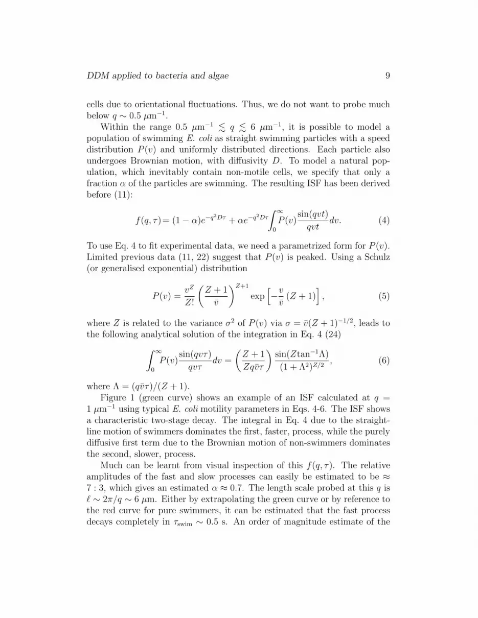
Much can be learnt from visual inspection of this f(q, τ). The relativeamplitudes of the fast and slow processes can easily be estimated to be ≈7 : 3, which gives an estimated α ≈ 0.7. The length scale probed at this q is` ∼ 2π/q ∼ 6 µm. Either by extrapolating the green curve or by reference tothe red curve for pure swimmers, it can be estimated that the fast processdecays completely in τswim ∼ 0.5 s. An order of magnitude estimate of the

DDM applied to bacteria and algae 10

swimming speed is therefore v ∼ `/τswim ∼ 12 µm/s. The slower, diffusive,process decays completely in τdiff ∼ 20 s, so that an estimate of the diffusioncoefficient of the non-swimmers can be obtained from 6Dτdiff ∼ `2, givingD ∼ 0.35 µm2/s. These are credible estimates of the parameters used togenerate this ISF: v = 15 µm/s, D = 0.3 µm2/s, and α = 0.7.

3.2 DDM Results

Fig. 2a shows typical DICFs, g(q, τ), measured using DDM in the range0.45 ≤ q ≤ 2.22 µm−1 for a suspension of SS E.coli mutant ∆cheY. Themeasured g(q, τ) have a characteristic shape reminiscent of the calculatedf(q, τ) shown in Fig. 1 (Note the log-scale for the y-axis in Fig. 2a); indeed,Eq. 2 shows that g(q, τ) should take the shape of an (un-normalized) ‘up-side-down’ f(q, τ). Eq. 2 also shows that the value of g(q, τ) at small τ givesa measure of the camera noise parameter B(q), which is therefore seen to bemore or less q-independent. The total amplitude of g(q, τ) measures the pre-factor A(q), which evidently increases rapidly as q decreases. This reflectsthe strong q dependence of both the form factor of a single bacterium andthe contrast function of the microscope objective.

The above qualitative remarks can be quantified by fitting the measuredg(q, τ) using Eqs. 2, 4 & 6. From the fit, we extract the six parameters v,σ, D, α, A and B. The fitted functions A(q) and B(q) allow us to calculatef(q, τ) from the measured g(q, τ) via Eq. 2 (25), Fig. 2b.

The ISFs calculated from experimental data (especially those for q ≈1 µm−1) show the characteristic shape already encountered in the theoreticalISF shown in Fig. 1: a fast decay due to swimming, followed by a slowdecay due to diffusion. The identity of these two processes is confirmedby the different scaling of the time axis required to collapse the data atdifferent q values: the slow (diffusive) decay scales as q2τ , Fig. 3a, and thefast (swimming, or ballistic) decay scales as qτ , Fig. 3b.

A clear separation of the swimming and diffusive decays is important forrobust fitting of the ISF using Eq. 4. Such separation of time scales will beachieved if a cell takes much less time to swim the characteristic distanceprobed, ` = 2π/q, than to diffuse over the same distance (in the imageplane), i.e. τswim ∼ `/v � τdiff ∼ `2/4D, which requires q � qc ∼ v/D ∼20 − 50 µm−1 for typical E. coli values of v and D. All the data shown inFig. 2b fit comfortably into this regime (23).

Fig. 4 shows the fit parameters (v, σ, α,D,A,B) from Eq. 4-6 as functions

DDM applied to bacteria and algae 11

of q. A common feature, particularly evident in D(q), is the enhanced noiseat low q. This is because at low q, the long-time, diffusive part of f(q, τ) hasnot fully decayed yet in our time window, rendering it harder to determineD accurately. This can be improved by probing g(q, τ) over long times. Towithin experimental uncertainties, the motility parameters (v, σ, α,D) are allq independent for q & 1 µm−1, which suggests that our model, Eq. 4, is indeedable to capture essential aspects of the dynamics of a dilute mixture of non-motile and smooth swimming E. coli. Note that a fit using fixed D, over thefull q-range, results in q-independent motility parameters only when the valueused for D is within 10% of the value found in free fitting (data not shown).Averaging over q, in the range 0.5 / q / 2.2, yields v = 10.9 ± 0.3 µm/s,σ = 6.43± 0.04 µm/s, α = 0.585± 0.002 and D = 0.348± 0.003 µm2/s witherror bars being the standard deviation of the mean in all cases except for vwhere estimated error bars reflects the residual q dependence.

Note that the value of D = 0.35 µm2/s is higher than the value (6)of D = 0.30 µm2/s expected for a suspension of purely non-motile E. coliwith ”paralyzed” flagella (∆motA) with similar geometry as the wild type.This is due to an enhancement of the diffusion of non-motile cells (and othercolloidal-sized objects) in a suspension of motile organisms (6, 21). More-over, the fitting of D is dominated by the diffusion of non-motile organisms:changing our model from Eq. 4 to one in which the motile cells do not diffusedoes not change the results (data not shown).

We used a Schulz distribution for modelling P (v) for analytic conveniencein the integration of Eq. 4. In Fig. 5a we show the average speed obtainedby fitting with three different probability distributions. The results for theSchulz and log-normal distributions agree closely, but using a Gaussian formproduced noisier data and a significantly lower v. The latter is becauseP (v = 0) 6= 0 for the Gaussian distribution, strongly overestimating thenumber of slow swimmers. The presence of these spurious slow swimmersin turns renders it difficult to fit D, causing noisier data for all motilityparameters.

We were able to fit the data satisfactorily irrespective of whether brightfield, phase contrast or fluorescence imaging was used. However, phase-contrast imaging shows a better signal to noise ratio (A(q)/B(q)). In partic-ular, changing A(q) and B(q) by using a 20× phase-contrast objective (whichis suboptimal for our experiment) produced the same results in the relevantq range (data not shown).

DDM applied to bacteria and algae 12

3.3 Tracking results

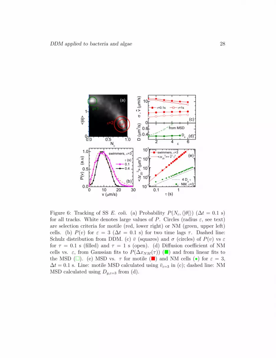
Figure 6(a) show the probability density of the track diagnostics (Nc, 〈|θ|〉)(Section 2.5). Recall that (Nc, 〈|θ|〉) = (1, 0) for straight swimming and(0, π/2) for Brownian diffusion. While two clear maxima corresponding todiffusion and (nearly-straight) swimming are observed, there is a substan-tial statistical weight of tracks with intermediate (Nc, 〈|θ|〉) values. The ac-tual distribution obtained depends on ∆t, the elementary time interval intowhich we segment trajectories. Our optimal choice, ∆t = 0.1s, over whichthe average swimming distance is ≈ 1 pixel, gave the most sharply sepa-rated peaks. However, the motile and NM populations are still not cleanlyseparated in our (Nc, 〈|θ|〉) data, Fig. 6a. We therefore select various pop-ulations of motile and NM cells by including tracks with (Nc, 〈|θ|〉) valueswithin progressively larger circles centered on their respective peaks in the(Nc, 〈|θ|〉) space. The radius of the circle (ε) is measured in units such thatthe (0 ≤ Nc ≤ 1, 0 ≤ 〈|θ|〉 ≤ π/2) space in Fig. 6a is a 10× 10 rectangle.

For motile cells, P (v) was determined, at each ε, by calculating the speed,v = 〈∆r2D(τ)/τ〉T , for each trajectory, averaged over the trajectory durationT , for various τ . The limit τ → 0 gives the instantaneous linear velocity. Inpractice, the lowest reasonable τ is set by ∆t = 0.1s. Figure 6b shows P (v) atε = 3 for τ = 0.1 s and 0.4 s, while Fig. 6c shows v and σ of P (v) for τ = 0.1 sand τ = 1 s. Unsurprisingly, v decreases with ε as progressively more ‘non-ideal’ swimming tracks are included: first more curved trajectories and then(at larger ε), some diffusive ones. Thus, there are ambiguities involved inmotility characterisation using tracking. It was also not possible to extractreliably a value for α due to strong dependence on ε.

However, the results for the other motility parameters show reasonableagreement with DDM (Fig. 4). In particular, using (∆t, τ) = (0.1s, 0.1s)(•, Fig. 6c), and averaging over all ε, v = 10.7 ± 0.3 µm/s and σ = 5.1 ±0.1 µm/s. The mean speed vε for each ε is also consistent with the MSDof the swimmers, Fig. 6e. The measured P (v) depends on τ , e.g. some fastswimmers will not be tracked for large τ unless perfectly aligned with theimage plane, while for very short τ the 2D-projection contributes to P (v) atsmall v (20). Yet, for τ ∼ 0.1 − 0.2s, our measured P (v) agrees with theSchulz distribution inferred from DDM, Fig. 6c.

For NM cells, we determined D by fitting the MSDs for selected tracks atseveral ε. We again found a dependence on (∆t, τ) and ε. The MSD for ε > 1showed deviations from purely diffusive behaviour and/or the resulting values

DDM applied to bacteria and algae 13

of D depend significantly on ε (Fig. 6d, �). Both effects are due to (likelyartificial) non-Gaussian tails in P (∆xNM(τ)) (not shown). Another estimateof the diffusion coefficient is Dg (based on Gaussian fits to P (∆xNM(τ)),Section 2.5), shown as a function of ε in Fig. 6d. The average value Dg =0.36 µm2/s agrees with the DDM value of 0.35 µm2/s and to the one fromthe MSD for ε = 1. Figure. 6e shows both the incorrect MSD of the diffusersobtained for ε = 3 and the appropriate MSD based on Dg.

3.4 Vertical motion and depth of field

Our derivation of Eq. 2 assumes that the image contrast of a bacterium doesnot vary with its position along the vertical (optical) z-axis, i.e. assumes aninfinite depth of field (δ). The validity of this assumption depends on howfast cells move relatively to the finite δ in reality. Giavazzi et al. presenteda complex theoretical model, based on the coherence theory, to take intoaccount this effect (8). Here, we suggest a simple model and use simulationsto investigate this effect and its importance over the accessible q-range. Oursimple model captures the essential features and reproduces qualitatively andquantitatively the experimental results.

Experimentally (6), the intensity profile of a bacterium along the z-axiscan be described by the contrast function

C(z) = CB − C0

(1− 4z2

δ2

)(7)

where CB and C0 are the background and the amplitude of an object inthe focal plane (z = 0) respectively. We determined CB and C0 experimen-tally, and then used this function to ‘smear’ the simulated data previouslypresented (6) to give simulated ‘images’ at a range of δ. At each δ exceptthe lowest, the input values {v, σ, α,D} are recovered from DDM analysisof these images at q & 2π/δ; the case of v is shown in Fig. 7. However, forq . 2π/δ, the analysis returns v and D values that are too high: disappear-ance of cells along the z axis due to the rapid fading of C(z) is mistaken asswimming and diffusion. Comparison between simulated data (Fig. 7) andexperimental data (Fig. 4 & 5b) shows that the effect of finite depth of field,δ, is negligible for q > 0.5 µm−1 using 10x phase-contrast imaging and thatour experimental depth of field δ & 20 µm.

DDM applied to bacteria and algae 14

4 Wild-Type E.coli

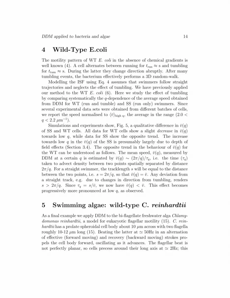
The motility pattern of WT E. coli in the absence of chemical gradients iswell known (4). A cell alternates between running for trun ≈ s and tumblingfor ttum ≈ s. During the latter they change direction abruptly. After manytumbling events, the bacterium effectively performs a 3D random-walk.

Modelling the ISF using Eq. 4 assumes that swimmers follow straighttrajectories and neglects the effect of tumbling. We have previously appliedour method to the WT E. coli (6). Here we study the effect of tumblingby comparing systematically the q-dependence of the average speed obtainedfrom DDM for WT (run and tumble) and SS (run only) swimmers. Sinceseveral experimental data sets were obtained from different batches of cells,we report the speed normalised to 〈v〉high q, the average in the range (2.0 <q < 2.2 µm−1).

Simulations and experiments show, Fig. 5, a qualitative difference in v(q)of SS and WT cells. All data for WT cells show a slight decrease in v(q)towards low q, while data for SS show the opposite trend. The increasetowards low q in the v(q) of the SS is presumably largely due to depth offield effects (Section 3.4). The opposite trend in the behaviour of v(q) forthe WT can be understood as follows. The mean speed, v(q), measured byDDM at a certain q is estimated by v(q) ∼ (2π/q)/τq, i.e. the time (τq)taken to advect density between two points spatially separated by distance2π/q. For a straight swimmer, the tracklength s will be equal to the distancebetween the two points, i.e. s = 2π/q, so that v(q) = v. Any deviation froma straight track, e.g. due to changes in direction from tumbling, renderss > 2π/q. Since τq = s/v, we now have v(q) < v. This effect becomesprogressively more pronounced at low q, as observed.

5 Swimming algae: wild-type C. reinhardtii

As a final example we apply DDM to the bi-flagellate freshwater alga Chlamy-domonas reinhardtii, a model for eukaryotic flagellar motility (15). C. rein-hardtii has a prolate spheroidal cell body about 10 µm across with two flagellaroughly 10-12 µm long (15). Beating the latter at ' 50Hz in an alternationof effective (forward moving) and recovery (backward moving) strokes pro-pels the cell body forward, oscillating as it advances. The flagellar beat isnot perfectly planar, so cells precess around their long axis at ' 2Hz; this

DDM applied to bacteria and algae 15

rotation, critical to phototaxis (17), results in helical swimming trajectories.For length scales ∼ 100 µm the direction of the axis of the helical tracksis approximately straight, but on larger scales the stochastic nature of theflagellar beat causes directional changes resulting in random walk (5, 26, 27).

Racey et al. (28) carried out the first high-speed microscopic trackingstudy of C. reinhardtii, obtaining the cells’ swimming speed distribution,with mean speed v = 84µm/s, as well as the average amplitude A = 1.53µmand frequency f = 49 Hz of the beat. A more recent tracking study obtaineda 2D swimming speed distribution with v ≈ 100µm/s (29). The swimmingof C. reinhardtii has also been studied with dynamic light scattering (DLS)(28, 30). However, studies at appropriately small q are difficult, severelylimiting useful data (the limitation is even greater than for bacteria: algaeswim on larger length scales, requiring smaller values of q). We present herethe first characterisation of the swimming motility of C. reinhardtii usingDDM. As for E. coli, the technique allows to study the 3D motion of muchlarger numbers of cells (∼ 104) than tracking, and allows easy access to largerlength scale than DLS.

5.1 Model of f(q, τ)

The swimming dynamics of C. reinhardtii are on larger length scales, shortertime scale (algae swim faster) and of a different nature than E. coli, somodels and experimental conditions used for DDM need to be adjusted forthis organism. In particular, the decay of the ISF, f(q, τ), will reflect thesealgae’s peculiar dynamics. Cells oscillate at lengthcales < 10µm, translatein the range 10µm < L < 30µm, spiral over 30µm < L < 100µm, anddiffuse for L > 100µm. A schematic representation of a helical trajectory,highlighting the small scale oscillatory motion is shown in inset of Fig. 8(diffusive length scales are not shown).

At length scales L / 30 µm, the swimming of C. reinhardtii can beapproximated as a sinusoidal oscillation superimposed on a linear progression,so that the particle displacement ∆r(τ) of a cell after a time interval τ isgiven by (30)

∆r(τ) = vτ + A0[sin(2πf0τ + φ)− sin(φ)], (8)

where A0 and f0 are the amplitude and frequency of the swimming oscillationand φ is a random phase to ensure the swimming beats of different cells

DDM applied to bacteria and algae 16

are not synchronised. Substituting this into Eq. 3, averaging over φ, andassuming a Schulz distribution for the swimming speed (Eq. 5), we obtainthe ISF,

falgae(q, τ) =1

2

∫ 1

−1

cos [(Z + 1) tan−1 (Λχ)][1 + (Λχ)2](Z+1)/2

J0[2qA0χ sin(πf0τ)] dχ, (9)

where Λ ≡ qvτZ+1

, χ ≡ cosψ, where ψ is the angle between ~q and ~r, J0 isthe zeroth order Bessel function. All other terms are as previously defined.The first and second term describe the contribution from straight swimmingand oscillatory beat, respectively. In the limit qA0 � 1 (J0 → 1), Eq. 9analytically integrates to Eq. 6, the same expression as for the progressivemodel used for E. coli.

The derivation of Eq. 9 assumes the distributions P (A) and P (f) forswimming amplitude and frequency, respectively, are narrowly centred aroundthe values A0 and f0 and ignores (i) the negligible diffusion of non-motile al-gae; (ii) any bias in the swimming direction caused by gravitaxis (31); and(iii) the helical nature of the swimming.

5.2 DDM results

Fig. 8a shows a typical DICF, g(q, τ), at q = 0.52 µm−1 (l ≈ 12 µm), fora suspension of WT alga C. reinhardtii measured using DDM. The recon-structed ISFs, f(q, τ), are shown in Fig. 8b in the range 0.2 / q / 0.9 µm−1,corresponding to a length scale range of 7 / l / 30 µm−1. f(q, τ) showsa characteristic shape for all q’s: a fast decay at τ ≤ 0.02 s due to theoscillatory beat and a slower decay at τ ≥ 0.02 s due to swimming. Theidentity of these two processes is confirmed by their difference in τ− and q−dependencies. The characteristic time of the fast process is independent ofq, while its amplitude decreases with q. Both observations fully agree withthe term (J0) due to the oscillatory contribution in Eq. 9. Moreover, 0.02 scorresponds to the period of a 50 Hz oscillatory beat. Finally, the slow pro-cess scales perfectly with qτ (data not shown) confirming the ballistic nature(swimming) of this process.

Fig. 9 shows the fitting parameters (v, σ, A0, f0) from Eq. 2 using the os-cillatory model (Eq. 9) as a function of q. All parameters display a smallq-dependence. This is likely due to effects not captured by the simple oscilla-tory model (e.g. body precession and helical swimming) and will be discussed

DDM applied to bacteria and algae 17

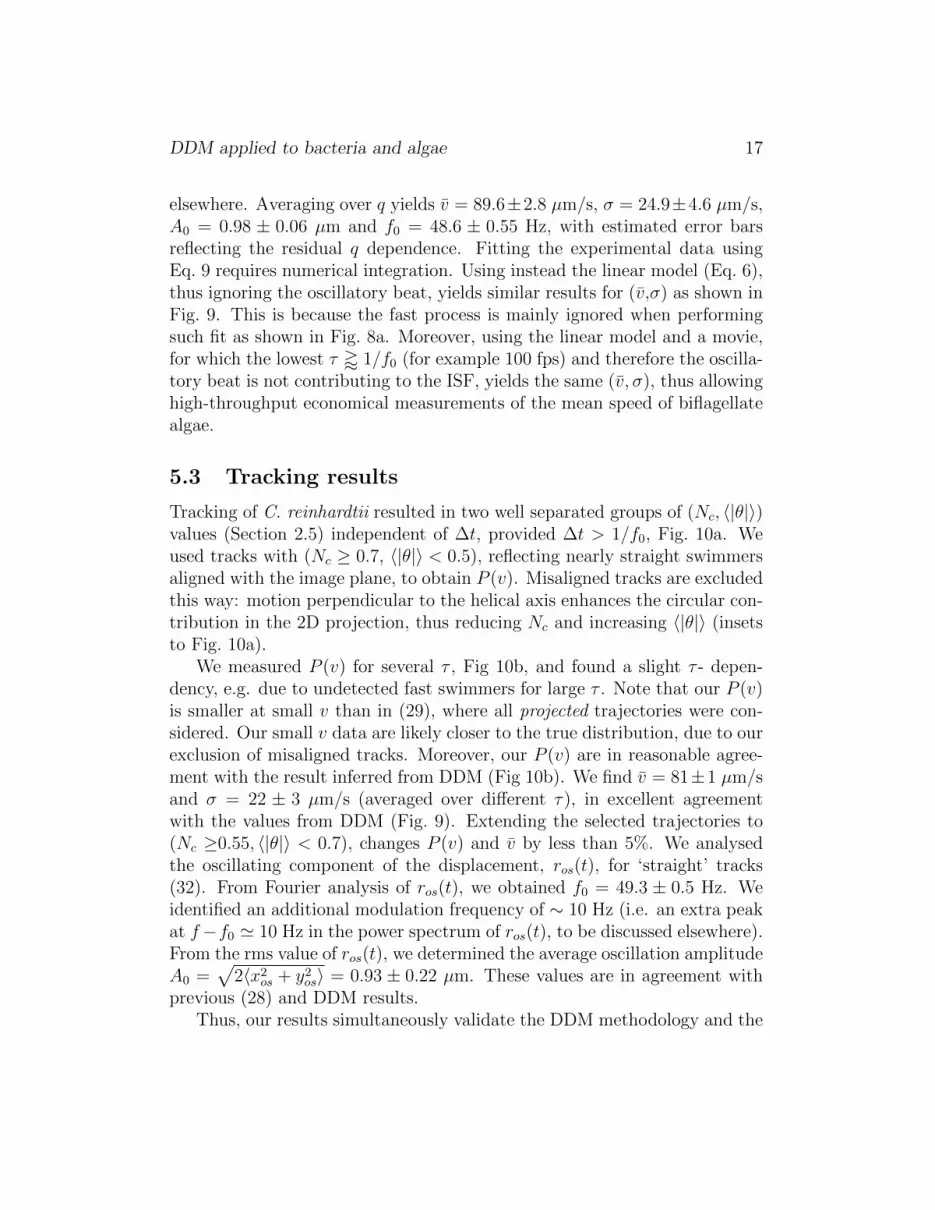
elsewhere. Averaging over q yields v = 89.6±2.8 µm/s, σ = 24.9±4.6 µm/s,A0 = 0.98 ± 0.06 µm and f0 = 48.6 ± 0.55 Hz, with estimated error barsreflecting the residual q dependence. Fitting the experimental data usingEq. 9 requires numerical integration. Using instead the linear model (Eq. 6),thus ignoring the oscillatory beat, yields similar results for (v,σ) as shown inFig. 9. This is because the fast process is mainly ignored when performingsuch fit as shown in Fig. 8a. Moreover, using the linear model and a movie,for which the lowest τ ' 1/f0 (for example 100 fps) and therefore the oscilla-tory beat is not contributing to the ISF, yields the same (v, σ), thus allowinghigh-throughput economical measurements of the mean speed of biflagellatealgae.

5.3 Tracking results

Tracking of C. reinhardtii resulted in two well separated groups of (Nc, 〈|θ|〉)values (Section 2.5) independent of ∆t, provided ∆t > 1/f0, Fig. 10a. Weused tracks with (Nc ≥ 0.7, 〈|θ|〉 < 0.5), reflecting nearly straight swimmersaligned with the image plane, to obtain P (v). Misaligned tracks are excludedthis way: motion perpendicular to the helical axis enhances the circular con-tribution in the 2D projection, thus reducing Nc and increasing 〈|θ|〉 (insetsto Fig. 10a).

We measured P (v) for several τ , Fig 10b, and found a slight τ - depen-dency, e.g. due to undetected fast swimmers for large τ . Note that our P (v)is smaller at small v than in (29), where all projected trajectories were con-sidered. Our small v data are likely closer to the true distribution, due to ourexclusion of misaligned tracks. Moreover, our P (v) are in reasonable agree-ment with the result inferred from DDM (Fig 10b). We find v = 81±1 µm/sand σ = 22 ± 3 µm/s (averaged over different τ), in excellent agreementwith the values from DDM (Fig. 9). Extending the selected trajectories to(Nc ≥0.55, 〈|θ|〉 < 0.7), changes P (v) and v by less than 5%. We analysedthe oscillating component of the displacement, ros(t), for ‘straight’ tracks(32). From Fourier analysis of ros(t), we obtained f0 = 49.3 ± 0.5 Hz. Weidentified an additional modulation frequency of ∼ 10 Hz (i.e. an extra peakat f−f0 ' 10 Hz in the power spectrum of ros(t), to be discussed elsewhere).From the rms value of ros(t), we determined the average oscillation amplitudeA0 =

√2〈x2

os + y2os〉 = 0.93 ± 0.22 µm. These values are in agreement with

previous (28) and DDM results.Thus, our results simultaneously validate the DDM methodology and the

DDM applied to bacteria and algae 18

simple model (Eq. 8 & 9) for the swimming of C. reinhardtii. Our methodcan therefore be used for the fast and accurate characterisation of the motilityof large ensembles of this organism, and, potentially, of other algae.

Conclusions

We have shown that DDM is a powerful, high-throughput technique to char-acterise the 3D swimming dynamics of microorganisms over a range of timescales and length scales (∼ 3 and ∼ 1 order of magnitude respectively) si-multaneously in a few minutes, based on standard imaging microscopy. Thetime scales and length scales of interest depend on the swimming dynamicsof the microorganism, and are easily tuned by changing the frame rate oroptical magnification respectively.

We have studied in considerable detail how to use DDM for character-ising the motility of smooth-swimming (run only) and wild-type (run andtumble) E. coli, as well as the wild-type alga C. reinhardtii. We validatedthe methodology using tracking and simulations. The latter was also usedto investigate the effect of a finite depth of field and tumbling. Using DDM,we were able to extract (i) for E. coli: the swimming speed distribution, thefraction of motile cells and the diffusivity; and (ii) for C. reinhardtii: theswimming speed distribution, the amplitude and frequency of the oscillatorydynamics. In both cases, these parameters were obtained by averaging overmany thousands of cells in a few minutes without the need for specialisedequipment.

Further developments are possible. For E. coli, analytic expressions forv(q) taking into account either trajectory curvature due to rotational Brown-ian motion (smooth swimmers) or directional changes due to tumbling (wildtype), can be derived. Fitting these expressions to data should then yieldquantitative information on the respective features. For C. reinhardtii, thehelical motion, the asymmetric nature of the swimming stroke, and the higherharmonics in the body oscillations observed by tracking could be exploredtheoretically and using DDM experiments. This will allow us to test sim-ulations that use the method of regularised stokeslets to reproduce the finedetails of the swimming of bi-flagellate algae (33).

DDM is based on the measurement of the spatio-temporal fluctuationsin intensity, and therefore does not require good optical resolution of themotile objects. Thus, DDM can probe a large field of view, yielding good

DDM applied to bacteria and algae 19

statistics even under relatively poor imaging conditions. Moreover, DDMcould also be used to probe anisotropic or asymmetric dynamics (34) ofmicroorganisms. Finally, the analysis is not restricted to dilute suspensionsand can be used to investigate the swimming dynamics at different timescales and length scales of the collective behaviour of populations. However,quantitative interpretation of the resulting data will require new models ofthe ISF.

With the availability of DDM, quantitative characterisation of motilitycan become a routine laboratory method, provided suitable theoretical mod-els are available for fitting of the ISF. Even without such models, however,qualitative features of the measured ISF can still allow conclusions to bedrawn and trends to be studied (e.g. the speeding up of the decay of the ISFalmost invariably correspond to faster motion). DDM should therefore be apowerful tool in future biophysical studies of microorganismic locomotion.

Acknowledgment

Authors acknowledge support from FP7-PEOPLE (PIIF-GA-2010-276190);EPSRC (EP/D073398/1); the Carnegie Trust for the Universities of Scotland;the Swiss National Science Foundation (PBFRP2-127867 and 200021-127192)and EPSRC (EP/E030173/1 and EP/D071070/1).

References

1. Yoshiyama, H., and T. Nakazawa. 2000. Unique mechanism of Heli-cobacter pylori for colonizing the gastric mucus. Microbes and Infection,2, 55-60.

2. Berg, H.C. 2004. E. coli in motion. Springer.

3. Berg, H.C. 1971. How to track bacteria. Rev. Sci. Instr., 42, 868-871.

4. Berg, H.C. and D.A. Brown. 1972. Chemotaxis in Escherichia coli anal-ysed by Three-dimensional Tracking. Nature, 239, 500-504.

5. Drescher, K., K.C. Leptos, and R.E. Goldstein. 2009. How to trackprotists in three dimensions. Rev. Sci. Instrum. 80:014301.

DDM applied to bacteria and algae 20

6. Wilson, L.G., V.A. Martinez, J. Schwarz-Linek, J. Tailleur, G. Bryant,P.N. Pusey and W.C.K. Poon. 2011. Differential Dynamic Microscopyof Bacterial Motility. Phys. Rev. Lett., 106:018101.

7. Cerbino, R., and V. Trappe. 2008. Differential Dynamic Microscopy:Probing Wave Vector Dependent Dynamics with a Microscope. Phys.Rev. Lett., 100:188102.

8. Giavazzi, F., D. Brogioli, V. Trappe, T. Bellini and R. Cerbino. 2009.Scattering information obtained by optical microscopy: Differential dy-namic microscopy and beyond Phys. Rev. E, 80:031403.

9. Boon, J.P., R. Nossal and S.H. Chen. 1974. Light-scattering spectrumdue to wiggling motions of bacteria. Biophys. J., 14:847–864.

10. Berne, B.J. and R. Pecora. 2000. Dynamic Light Scattering, Dover.

11. Stock, G.B. 1978. The measurement of bacterial translation by photoncorrelation spectroscopy. Biophys. J., 22:79–96.

12. P1 phage transduction (13) was used to create a smooth swimming(AB1157 ∆cheY) using the appropriate E. coli K-12 single knockoutmutant from the KEIO collection (14). Kanamycin (final concentration30 mg/l) was added to all growth media for AB1157 ∆cheY.

13. Miller, J.H. 1972. Experiments in Molecular Genetics. Cold Spring Har-bor Laboratory Press.

14. Baba, T., T. Ara, M. Hasegawa, Y. Takai, Y. Okumura, M. Baba, K.A.Datsenko, M. Tomita, B.L. Wanner and H. Mori. 2006. Construction ofEscherichia coli K-12 in-frame, single-gene knockout mutants: the Keiocollection. Mol. Syst. Biol., 2, 111.

15. Harris, E.H. 2009. The Chlamydomonas sourcebook. Academic Press.

16. Croze, O.A., E.E. Ashraf, and M.A. Bees. 2010. Sheared bioconvectionin a horizontal tube. Phys. Biol. 7:046001.

17. Foster, K.W. and R.D. Smyth. 1980. Light antennas in phototactic algae.Microbiol. Rev. 44:572–630.

18. All relevant softwares are available on request.

DDM applied to bacteria and algae 21

19. Crocker, J.C. and D.G Grier. 1996. Methods of digital video microscopyfor colloidal studies J. Coll. Int. Sci., 179:298–310.

20. 2D tracking measures P (v cos(β)) (β is the angle with the image plane)rather than P (v), but this has only a small effect on the results. Bytracking only the brightest features within z of the focal plane, onlytracks with τv sin(β) < z contribute, which supresses projection effects.Moreover, the diagnostic method to select ’straight’ swimmers, presentedlater, further excludes large β tracks from the motile population, sincethese tracks exhibit a stronger diffusive (E. coli) or circular component(algae), a result of the projection.

21. Mino, G., T.E. Mallouk, T.Darnige, M. Hoyos, J. Dauchet, J. Dunstan,R. Soto, Y. Wang , A. Rousselet and E. Clement. 2011. Enhanceddiffusion due to active swimmers at a solid surface Phys. Rev. Lett.,106:048102.

22. Nossal, R., S.H. Chen and C.C. Lai. 1971. Use of laser scattering forquantitative determinations of bacterial motility. Opt. Commun., 4:35–39.

23. In the regime of q � qc, the ISF separates into a fast diffusive processfollowed by a slower swimming process.

24. Pusey, P.N. and W. van Megen. 1984. Detection of small polydispersitiesby photon correlation spectroscopy J. Chem. Phys., 80:3513–3520.

25. The determination of A(q) and B(q) does not necessarily requires fit-ting of g(q, τ) and therefore a model for f(q, τ). They could simplybe determined from the short and long time limit of g(q, τ) such as:B(q) = f(q, τ → 0) and A(q) = f(q, τ → ∞) − B(q). However, the lat-ter requires well-defined ”plateau” at both short and long time regimes,which are not always observed depending on the value of q, and the ex-perimental time window restricted: at short-time by the frame rate andat long-time by the duration of the movie.

26. Hill, N.A. and T.J. Pedley. 2005. Bioconvection. Fluid. Dyn. Res., 37:1–20.

DDM applied to bacteria and algae 22

27. Polin, M., I. Tuval, K. Drescher, J.P. Gollub and R.E. Goldstein. 2009.Chlamydomonas swims with two ”gears” in a eukaryotic version of run-and-tumble locomotion. Science, 325:487–490.

28. Racey, T.J., R. Hallett and B. Nickel. 1981. A quasi-elastic light scatter-ing and cinematographical investigation of motile Chlamydomonas rein-hardtii. Biophys. J., 35:557–571.

29. K.C. Leptos, J.S. Guasto, J.P. Gollub,A.I. Pesci and R.E. Goldstein.2009. Dynamics of Enhanced Tracer Diffusion in Suspensions of Swim-ming Eukaryotic Microorganisms Phys. Rev. Lett., 103:198103.

30. T.J. Racey and F.R. Hallett, 1983. A low angle quasi-elastic light scat-tering investigation of Chlamydomonas reinhardtii J. Musc. Res. Cell.Motil., 4:321–331.

31. N.A. Hill and D.P. Hader. 1997. A Biased Random Walk Model for theTrajectories of Swimming Micro-organisms J. Theor. Biol., 186:503–526.

32. We define ros(t) = (xos, yos)(t) = r2D(t)−〈r2D(t)〉dt with dt = 2/f0. ros(t)is well resolved due to subpixel accuracy ∼ 0.2 µm of the coordinates.

33. O’Malley, S. and M.A. Bees, 2011. The Orientation of Swimming Biag-ellates in Shear Flows Bull. Math. Bio., 74:232–255.

34. Reufer, M., V.A. Martinez, P. Schurtenberger and W.C.K. Poon.2012. Differential dynamic microscopy for anisotropic colloidal dynamics.Langmuir. In press.

DDM applied to bacteria and algae 23

timeI(r,t1)

r

ti+t

t1

ti

Di(r,t)= I(r,ti + t) - I(r,ti)FFT,

FD (q,t)2

. 2

LxL pixels

.

q

ig(q,t)

ti. g(q,t)q

(b)

Figure 1: (a) Theoretical ISF, f(q, τ), vs τ at q = 1 µm−1, for (black dottedline) a population of diffusing spheres with D = 0.3 µm2/s, (red dashedline) a population of equivalent-size spheres swimming isotropically in 3Dwith a Schulz speed distribution P (v) with average speed v = 15 µm/sand width σ = 7.5 µm/s, and (green line) a 30:70 mixture of diffusers andswimmers. (b) Schematic of the image processing to obtain the DICFs,g(q, τ), from the videos (left) collected in an experiment. (Middle) Non-averaged image, |FDi(~q, τ)|2 and (right) averaged image, g(~q, τ), over initialtimes ti at τ = 0.52 s.

DDM applied to bacteria and algae 24

46

106

2

46

107

2

4

g(q,

)

q (µm-1) 0.45 0.67 0.90 1.12 1.34 1.56 1.79 2.01 2.22

(a)

1.0

0.8

0.6

0.4

0.2

0.0

f(q,

)

10-2

10-1

100

101

Delay Time (s)

(b)

Figure 2: DDM for smooth swimming E. coli. (a) Measured (symbols) andfitted (lines) DICFs, g(q, τ). (b) ISFs, f(q, τ), reconstructed from g(q, τ)using Eqs. 2,4 & 6.

DDM applied to bacteria and algae 25

1.0

0.8

0.6

0.4

0.2

0.0

f(q,

)

10-2

10-1

100

101

q (s / µm)

(a)

1.0

0.8

0.6

0.4

0.2

0.0

f(q,

)

10-3

10-2

10-1

100

101

102

q2

(s / µm2)

(b)

Figure 3: The reconstructed ISFs, f(q, τ), shown in Fig. 2 plotted against(a) qτ and (b) q2τ . Data collapse for the fast process in (a) and for the slowprocess in (b). q value increases from red to blue end of the spectrum colourin the range 0.3 ≤ q ≤ 2.2 µm−1.

DDM applied to bacteria and algae 26

141210v

(µ

108642

µ

0.80.60.40.2

0.80.60.40.2D

(µ

105

107

A(q

), B

(q)

2.01.51.00.50.0

q (µ

Figure 4: SS E. coli. Fitting parameters vs q using Eqs. 2, 4 & 6. From topto bottom: v and σ of the Schulz distribution, motile fraction α, diffusivityD, and A(q) (◦) and B(q) (�). Red lines are results from tracking, withthickness corresponding to the error bars. No reliable value for α could beobtained from tracking.

DDM applied to bacteria and algae 27

µ

µ

µ

Figure 5: Swimming speed vs. q from DDM. (a) Effect of using differentforms of the speed distribution: lognormal (�), Schulz (◦), and Gaussian(4). (b) Effect of tumbling (experiments): four data sets from the SS (blacksymbols) and four data sets from the WT (red symbols). (c) Effect of tum-bling (simulations): SS (◦) and WT (�). Note that for (b) and (c) panels,the swimming speed has been normalised to 〈v〉high q to enable comparisonand highlight the difference in q-dependence.

DDM applied to bacteria and algae 28

Figure 6: Tracking of SS E. coli. (a) Probability P (Nc, 〈|θ|〉) (∆t = 0.1 s)for all tracks. White denotes large values of P . Circles (radius ε, see text)are selection criteria for motile (red, lower right) or NM (green, upper left)cells. (b) P (v) for ε = 3 (∆t = 0.1 s) for two time lags τ . Dashed line:Schulz distribution from DDM. (c) v (squares) and σ (circles) of P (v) vs εfor τ = 0.1 s (filled) and τ = 1 s (open). (d) Diffusion coefficient of NMcells vs. ε, from Gaussian fits to P (∆xNM(τ)) (�) and from linear fits tothe MSD (�). (e) MSD vs. τ for motile (�) and NM cells (•) for ε = 3,∆t = 0.1 s. Line: motile MSD calculated using vε=3 in (c); dashed line: NMMSD calculated using Dg,ε=3 from (d).

DDM applied to bacteria and algae 29

µm-1

)

(µm) 5 10 20 40 75 100

Figure 7: Effect of the depth of field on DDM analysis of simulated data.Normalised mean swimming speed v/vinput versus q for smooth swimmersand several values of depth of field δ. vinput = 15µm/s is the input meanswimming speed used to generate the simulated data.

DDM applied to bacteria and algae 30

7x106

6

5

4

3

2

1

g(q,

)

q=0.54 µm-1

Eq. 3 & 7 Eq. 3 & 10

(a)

1.0

0.8

0.6

0.4

0.2

0.0

f(q,

)

10-3

2 4 6 8

10-2

2 4 6 8

10-1

2

(s)

q (µm-1

) 0.18 0.27 0.36 0.45 0.54 0.63 0.72 0.81 0.89

(b)

Lo

Lp50 Hz

2 Hz

Lo

Lp50 Hz

2 Hz

Figure 8: DDM for WT C. reinhardtii. (a) Measured (circles) g(q, τ). Lineand dashed line are fits using the oscillatory model (Eq. 9) and the linearmodel (Eq. 6), respectively. Inset: Portion of a helical C. reinhardtii tra-jectory. The progressive, Lp, and (zoomed-in) oscillatory, L0, length scalesprobed by DDM are shown, with the frequencies of the helical precession(2 Hz) and oscillatory swimming (50 Hz). (b) ISFs, f(q, τ), using Eqs. 2 &9.

DDM applied to bacteria and algae 31

1101009080v

(µm

/s)

40

20 (µm

/s)

1.5

1.0

A0

(µm

)

50

45

40

f 0 (H

z)

0.90.80.70.60.50.40.30.2

q (µm-1

)

Figure 9: Fitting parameters using the oscillatory model Eq. 9 (circles) orlinear model Eq. 6 (squares) as function of q for C. reinhardtii. From top tobottom: v and σ of the Schulz distribution, amplitude A0, and frequency f0.Red lines are results from tracking with dashed lines corresponding to errorbars.

Figure 10: Tracking of C. reinhardtii. (a) Probability P (Nc, 〈|θ|〉) of all tracks(∆t = 0.05 s). Tracks within the red bordered region (example in top rightinset, 7 s, scalebar 150 µm) are used to measure P (v); Top left inset: anexcluded track with Nc < 0.4 (30 s, scalebar 30 µm). (b) Normalised P (v)from tracks selected in (a), for two values of τ . Dashed line: P (v) from DDManalysis.