Differential Pulse Code ModulationDifferential Pulse Code ModulationDPCMDPCM

Introduction

General block diagram

Bi-dimensional prediction

DPCM distortions

Examples

Lossless coding scheme

Application to motion estimation (introduction)

Thanks for material provided

Inald Lagendijk, Delft University of TechnologyThomas Wiegand, Heinrich-Hertz-Institut

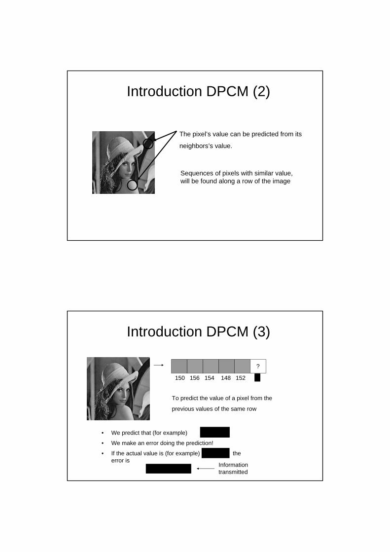
IntroductionIntroduction DPCM (1)DPCM (1)First technique of image coding (~1952)

500 1000 1500 2000 2500 3000 3500 4000 4500100

0

100

∆x(

n)=

x(n)

-x(n

-1) 0 500 1000 1500 2000 2500 3000 3500 4000 450050

100

150

200

250

x(n

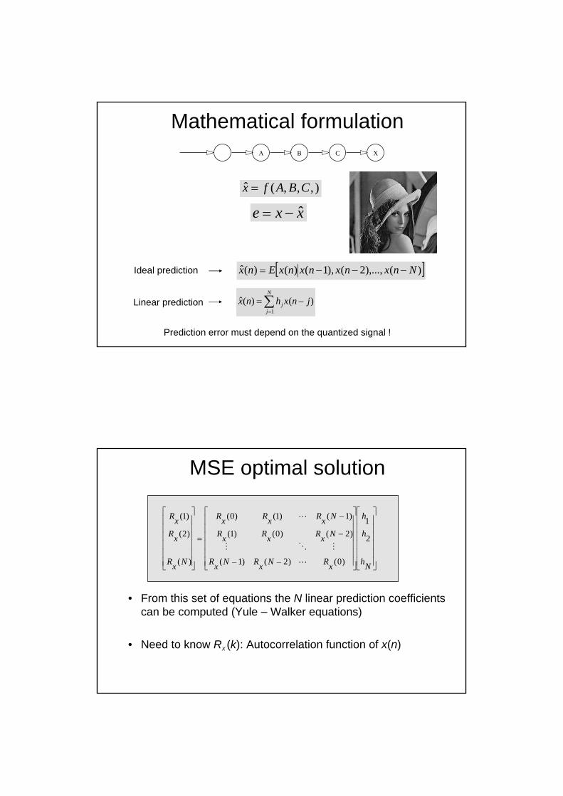
IntroductionIntroduction DPCM DPCM (2)(2)

The pixel’s value can be predicted from its

neighbors’s value.

Sequences of pixels with similar value, will be found along a row of the image

IntroductionIntroduction DPCM DPCM (3)(3)

150 156 154 148 152

?

To predict the value of a pixel from the

previous values of the same row

• We predict that (for example)

• We make an error doing the prediction!

• If the actual value is (for example) the error is

x̂

150ˆ =x

149=x

1ˆ −=−= xxe Informationtransmitted

A X

MathematicalMathematical formulationformulationB C

),,,(ˆ CBAfx =

xxe ˆ−=

[ ])(),...,2(),1()()(ˆ NnxnxnxnxEnx −−−=Ideal prediction

)()(ˆ1

jnxhnxN

jj −= ∑

=Linear prediction

Prediction error must depend on the quantized signal !

MSE optimal solutionMSE optimal solution

RxRx

Rx N

Rx Rx Rx N

Rx Rx Rx N

Rx N Rx N Rx

h

h

hN

( )

( )

( )

( ) ( ) ( )

( ) ( ) ( )

( ) ( ) ( )

1

2

0 1 1

1 0 2

1 2 0

1

2

⎡

⎣

⎢⎢⎢⎢⎢⎢

⎤

⎦

⎥⎥⎥⎥⎥⎥

=

−

−

− −

⎡

⎣

⎢⎢⎢⎢⎢⎢

⎤

⎦

⎥⎥⎥⎥⎥⎥

⎡

⎣

⎢⎢⎢⎢⎢⎢

⎤

⎦

⎥⎥⎥⎥⎥⎥

L

M O M

L

• From this set of equations the N linear prediction coefficients can be computed (Yule – Walker equations)

• Need to know RX (k): Autocorrelation function of x(n)

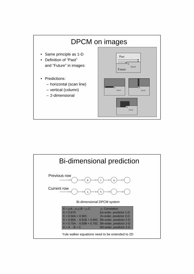
DPCM on imagesDPCM on images• Same principle as 1-D• Definition of “Past”

and “Future” in images:

• Predictions:– horizontal (scan line)– vertical (column)– 2-dimensional

B C D

A X

Bi-dimensional DPCM system

X = ρhA - ρh ρvB + ρvC ρ: CorrelationX = 0.97A 1st-order, predictor 1-D X = 0.50A + 0.50C 2n-order, predictor 2-DX = 0.90A - 0.81B + 0.90C 3th-order, predictor 2-D X = 0.75A - 0.50B + 0.75C 3th-order, predictor 2-D X = A - B + C 3th-order, predictor 2-D

BiBi--dimensionaldimensional predictionprediction

Previous row

Current row

Yule walker equations need to be extended to 2D

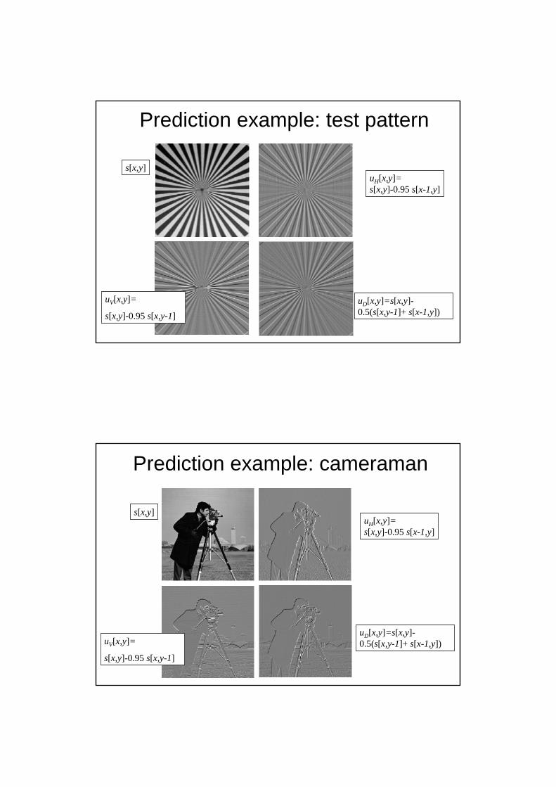
Prediction example: test patternPrediction example: test pattern

s[x,y]

uV[x,y]=

s[x,y]-0.95 s[x,y-1]

uH[x,y]=s[x,y]-0.95 s[x-1,y]

uD[x,y]=s[x,y]-0.5(s[x,y-1]+ s[x-1,y])

Prediction example: cameramanPrediction example: cameraman

s[x,y]uH[x,y]=s[x,y]-0.95 s[x-1,y]

uV[x,y]=

s[x,y]-0.95 s[x,y-1]

uD[x,y]=s[x,y]-0.5(s[x,y-1]+ s[x-1,y])

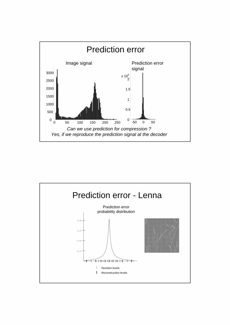
PredictionPrediction errorerror

0 50 100 150 200 2500

500

1000

1500

2000

2500

3000

Image signal Prediction errorsignal

Can we use prediction for compression ?Yes, if we reproduce the prediction signal at the decoder

-50 0 500

0.5

1

1.5

2x 104

PredictionPrediction error error -- LennaLennaPrediction error

probability distribution

0.10

0.20

0.30

0.40

Reconstruction levels

Decision levels

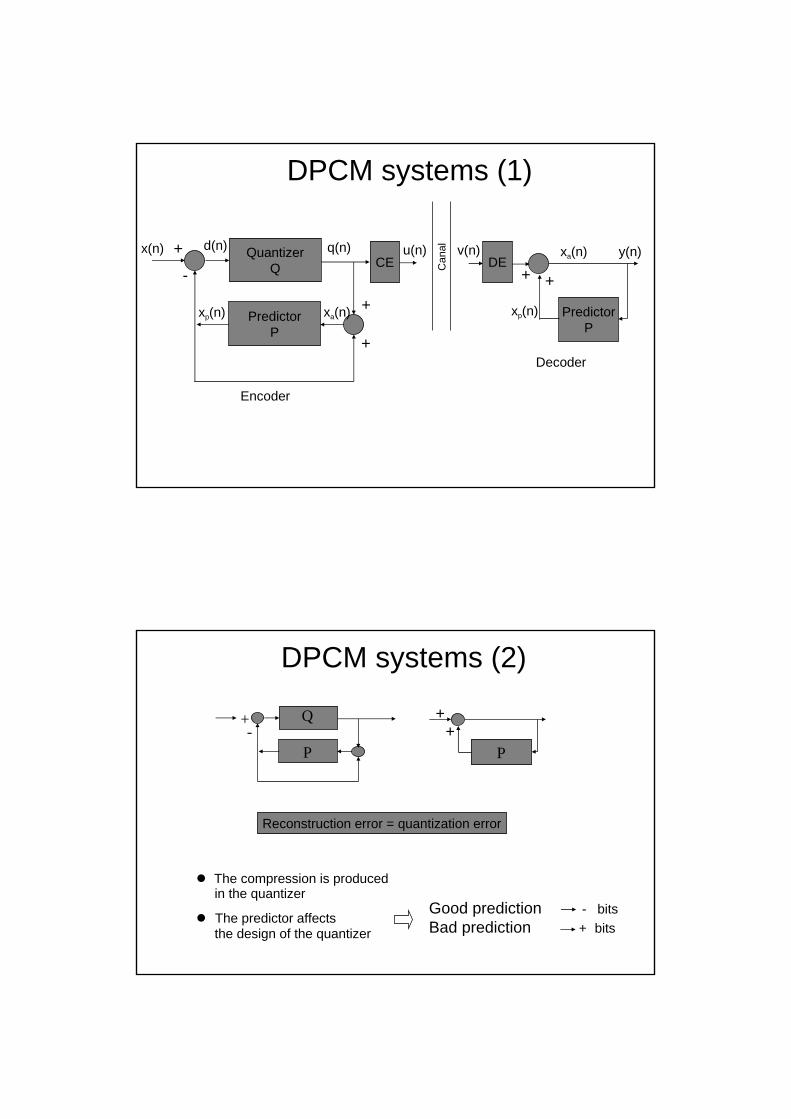
DPCM DPCM systems (systems (1)1)

PredictorP

++xa(n)

xp(n)

v(n) y(n)QuantizerQ

PredictorP

q(n)

+

+

+

-

d(n)x(n)

xp(n) xa(n)

Encoder

Decoder

CE DEu(n)

Can

al

DPCM DPCM systems (systems (2)2)

+-

Q

P P

Reconstruction error = quantization error

The compression is produced in the quantizer

The predictor affectsthe design of the quantizer

Good prediction - bitsBad prediction + bits

++

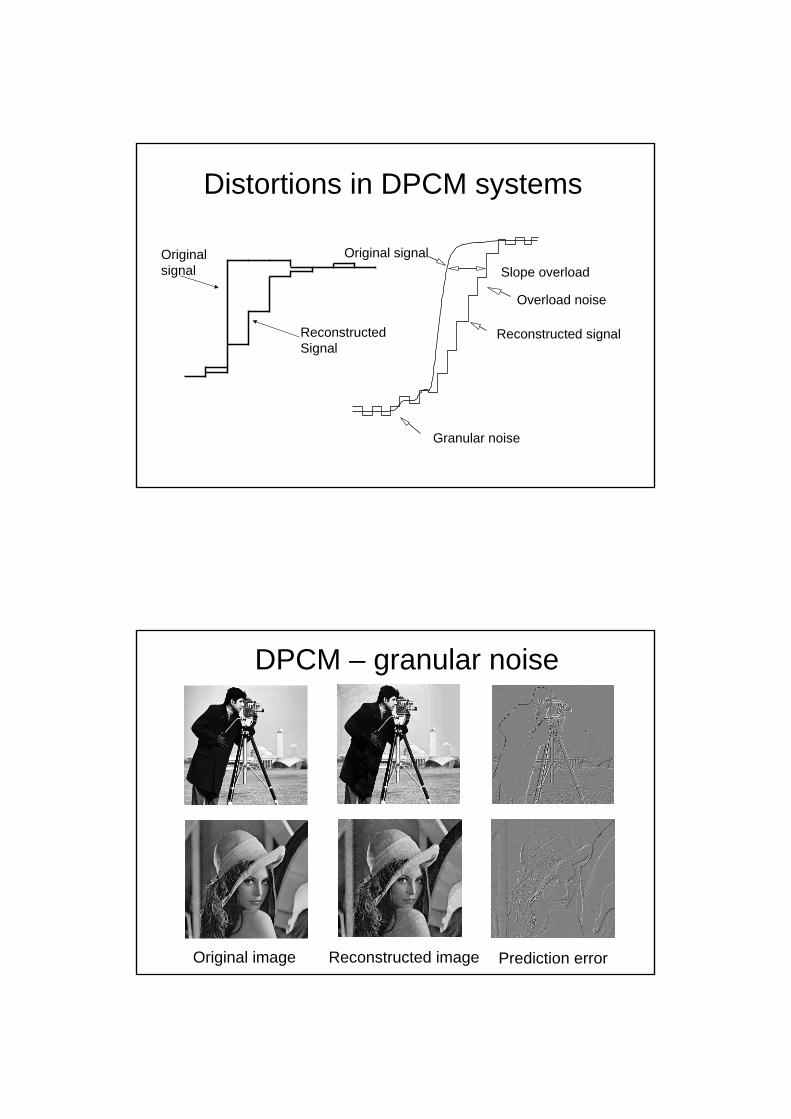
DistortionsDistortions in in DPCMDPCM systemssystems

Reconstructed signal

Original signalSlope overload

Granular noise

Overload noise

ReconstructedSignal

Original signal

DPCM DPCM –– granular granular noisenoise

Reconstructed image Prediction errorOriginal image

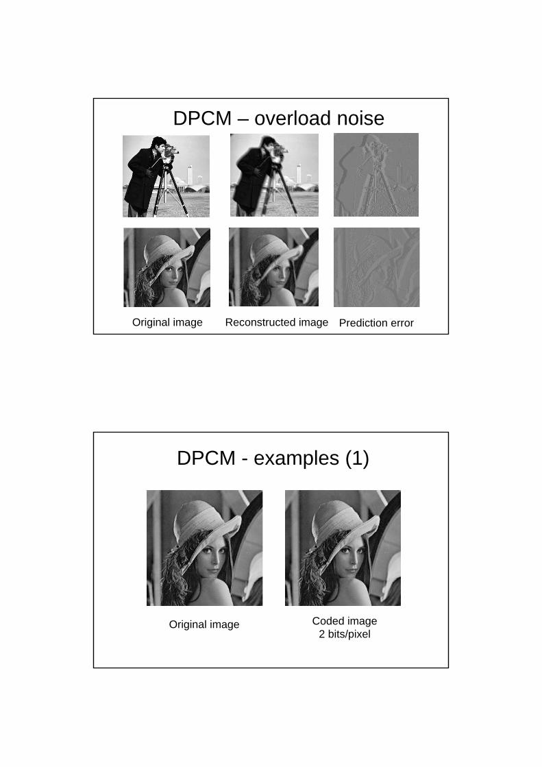
DPCM DPCM –– overloadoverload noisenoise

Reconstructed image Prediction errorOriginal image

DPCM DPCM -- examplesexamples (1)(1)

Original image Coded image2 bits/pixel

Prediction error1 bits/pixel

Prediction error2 bit/pixel

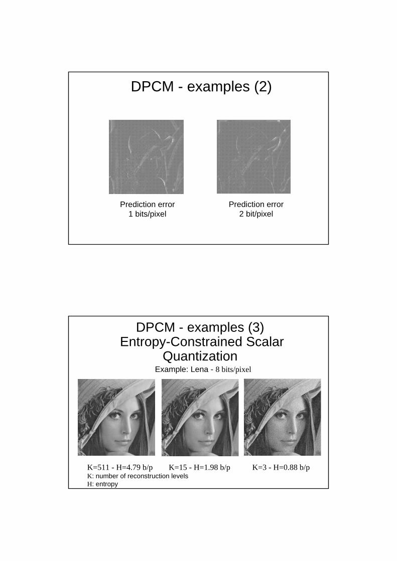
DPCM DPCM -- examplesexamples (2)(2)

DPCM DPCM -- examplesexamples (3)(3)EntropyEntropy--Constrained Scalar Constrained Scalar

QuantizationQuantization

K=511 - H=4.79 b/p K=15 - H=1.98 b/p K=3 - H=0.88 b/pK: number of reconstruction levelsH: entropy

Example: Lena - 8 bits/pixel

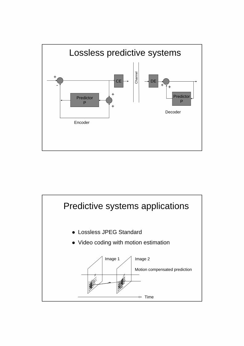
LosslessLossless predictivepredictive systemssystems

PredictorP

+

+

+

-

Encoder

CE

PredictorP

++

Decoder

DECha

nnel

PredictivePredictive systemssystems applicationsapplications

Lossless JPEG Standard

Video coding with motion estimation

Motion compensated prediction

Time

Image 1 Image 2