arX

iv:0

807.

4888

v3 [

mat

h.C

A]

21

Jan

2011

Dihedral Gauss hypergeometric functions

Raimundas Vidunas

Kobe University

January 24, 2011

Abstract

Gauss hypergeometric functions with a dihedral monodromy group can be ex-

pressed as elementary functions, since their hypergeometric equations can be trans-

formed to Fuchsian equations with cyclic monodromy groups by a quadratic change

of the argument variable. The paper presents general elementary expressions of

these dihedral hypergeometric functions, involving finite bivariate sums expressible

as terminating Appell’s F2 or F3 series. Additionally, trigonometric expressions for

the dihedral functions are presented, and degenerate cases (logarithmic, or with the

monodromy group Z/2Z) are considered.

1 Introduction

As well known, special cases of the Gauss hypergeometric function 2F1

(

A,BC

∣

∣

∣z)

can

be represented in terms of elementary functions. A particularly interesting case are

hypergeometric functions with a dihedral monodromy group; they can be expressed with

square roots inside power or logarithmic functions. The simplest examples are:

2F1

( a2, a+1

2

a+ 1

∣

∣

∣

∣

z

)

=

(

1 +√1− z2

)−a

, (1.1)

2F1

(

a2, a+1

2

1

2

∣

∣

∣

∣

∣

z

)

=(1 −√z)−a + (1 +

√z)−a

2, (1.2)

2F1

(

a+1

2, a+2

2

3

2

∣

∣

∣

∣

∣

z

)

=(1 −√z)−a − (1 +

√z)−a

2 a√z

(a 6= 0), (1.3)

2F1

(

1

2, 13

2

∣

∣

∣

∣

∣

z

)

=log(1 +

√z)− log(1 −√z)2√z

=arctan

√−z√−z , (1.4)

2F1

(

1

2, 1

2

3

2

∣

∣

∣

∣

∣

z

)

=log(√1− z +

√−z)√

−z =arcsin

√z√

z. (1.5)

These are solutions of the hypergeometric differential equation with the local exponent

differences 1/2, 1/2, a at the three singular points. The monodromy group is an infinite

1

dihedral group (for general a ∈ C), or a finite dihedral group (for rational non-integer

a), or an order 2 group (for non-zero integers a). We refer to Gauss hypergeometric

functions with a dihedral monodromy group as dihedral hypergeometric functions.

Despite a rich history of research of Gauss hypergeometric functions, only simplest

formulas for dihedral 2F1 functions like above are given in common literature [1, 15.1], [4,

2.8]. General dihedral 2F1 functions are contiguous to the simplest functions given above

(or their fractional-linear transformations); that is, their upper and lower parameters

differ by integers from the respective parameters of the simplest functions. The local

exponent differences of their hypergeometric equations are k + 1/2, ℓ + 1/2 and λ ∈ C,

where k, ℓ are integers.

An interesting problem is to find explicit elementary expressions for general dihedral

Gauss hypergeometric functions. A set of these expressions is presented in Sections 3,

4, 6 of this paper. The most general canonical expressions are given in Section 3, in

terms of terminating Appell’s F2 double sums. The key observation is that a particular

univariate specialization of Appell’s F2 function satisfies the same Fuchsian equation as

a quadratic transformation of general hypergeometric equations; see Theorem 2.1. When

the monodromy group of the hypergeometric equation is dihedral, the alluded F2 function

is a terminating double sum. Linear relations between dihedral 2F1 and terminating F2

solutions of the same Fuchsian equation give the announced elementary expressions for

the former.

Section 4 looks at the simpler case of dihedral hypergeometric equations with the local

monodromy differences k + 1/2, 1/2, λ. Then the terminating F2 doublesums become

terminating 2F1 sums. The case of the local exponent differences k + 1/2, k+ 1/2, λ can

be reduced to the described case by a quadratic transformation of the hypergeometric

equation.

Section 5 considers comprehensively degenerate cases with λ ∈ Z.

Section 6 considers trigonometric formulas for dihedral Gauss hypergeometric func-

tions. The simplest such expressions are [1, 15.1], [4, 2.8]:

2F1

(

a2, −a

2

1

2

∣

∣

∣

∣

∣

sin2 x

)

= cos ax, (1.6)

2F1

(

1+a2, 1−a

2

3

2

∣

∣

∣

∣

∣

sin2 x

)

=sin ax

a sinx. (1.7)

Supplementing paper [10] presents similar expressions (as double hypergeometric

sums) for quadratic invariants for hypergeometric equations with the dihedral mon-

odromy group, and describes rational pull-back transformations between dihedral hy-

pergeometric functions.

2

2 Preliminary facts

Basic facts on hypergeometric functions, Fuchsian equations, the monodromy group,

contiguous relations, terminating hypergeometric sums, Zeilberger’s algorithm are well

known. We suggest [2], [3], [5] as standard though overwhelming references. Wikipedia

pages [11] can be satisfactorily consulted for quick references.

2.1 The hypergeometric equation

The Gauss hypergeometric function 2F1

(

A, B

C

∣

∣

∣

∣

z

)

satisfies the hypergeometric differen-

tial equation [2, Formula (2.3.5)]:

z (1− z) d2y(z)

dz2+(

C − (A+ B + 1) z) dy(z)

dz−AB y(z) = 0. (2.1)

This is a canonical Fuchsian equation on P1 with three singular points. The singularities

are z = 0, 1,∞, and the local exponents are:

0, 1− C at z = 0; 0, C −A−B at z = 1; and A, B at z =∞.

The local exponent differences at the singular points are equal (up to a sign) to 1 − C,C −A−B and A− B, respectively. Let us denote a hypergeometric equation with the

local exponent differences d1, d2, d3 by E(d1, d2, d3), and consider the order of the three

arguments unimportant.

Because of frequent use, we recall Euler’s and Pfaff’s fractional-linear transformations

[2, Theorem 2.2.5]:

2F1

(

a, b

c

∣

∣

∣

∣

z

)

= (1− z)c−a−b2F1

(

c− a, c− bc

∣

∣

∣

∣

z

)

(2.2)

= (1− z)−a2F1

(

a, c− bc

∣

∣

∣

∣

z

z − 1

)

. (2.3)

The following quadratic transformation [2, (3.1.3),(3.1.9),(3.1.7)] will illustrate the

key reduction of the dihedral monodromy group to a cyclic monodromy group:

2F1

(

a, ba+b+1

2

∣

∣

∣

∣

x

)

= 2F1

(

a2, b

2

a+b+1

2

∣

∣

∣

∣

∣

4x (1 − x))

, (2.4)

2F1

(

a, b

a− b+ 1

∣

∣

∣

∣

x

)

= (1 + x)−a2F1

( a2, a+1

2

a− b + 1

∣

∣

∣

∣

4x

(1 + x)2

)

, (2.5)

2F1

(

a, b

2b

∣

∣

∣

∣

x

)

=(

1− x

2

)−a

2F1

(

a2, a+1

2

b+ 1

2

∣

∣

∣

∣

∣

x2

(2 − x)2

)

. (2.6)

The hypergeometric equations are related in the same way, by a quadratic pull-back

transformation of the form

z 7−→ ϕ(x), y(z) 7−→ Y (x) = θ(x) y(ϕ(x)), (2.7)

3

where ϕ(x) is a rational (quadratic in this case) function, and θ(x) is a power factor.

Geometrically, the transformation pull-backs the starting differential equation on the

projective line P1z to a differential equation on the projective line P1

x, with respect to

the covering ϕ : P1x → P1

z. The factor θ(x) shifts the local exponents of the pull-backed

equation, but it does not change the local exponent differences. We write the quadratic

transformation of hypergeometric equations as

E(

1

2, λ, µ

) 2←− E (λ, λ, 2µ) , (2.8)

as the local exponent differences 1/2, µ are doubled by the quadratic substitution, and the

point with the local exponent difference 1/2 becomes non-singular after an appropriate

choice of θ(x). The arrow follows the direction of the pull-back covering, as in [8], [10].

2.2 The monodromy group

The simplest hypergeometric equations with a dihedral monodromy group areE(1/2, 1/2, a).

The monodromy representation for these equations group can be computed using explicit

expressions (1.1)–(1.4). If a 6= 0, we take (1.2) and a√z times (1.3) as a basis of solutions;

analytic continuation along loops around z = 0 and z = 1 gives the following generators

of the monodromy group:(

1 0

0 −1

)

and

(

1+w2

1−w2

1−w2

1+w2

)

, w = exp(−2πia). (2.9)

If a = 0, the monodromy generators are

(

1 0

0 −1

)

and

(

1 2πi

0 1

)

.

In general, dihedral hypergeometric functions are contiguous to E(1/2, 1/2, a). They

are characterized by the property that their differences of local exponents at two of the

three singular points are half-integers. If the third local exponent is an irrational number,

the monodromy group is an infinite dihedral group; if it is a non-integer rational number,

the monodromy group is a finite dihedral group. If the third local exponent difference

is an integer, the monodromy group is isomorphic either to Z/2Z or (in presence of

logarithmic solutions) to an infinite dihedral group. The distinction of these two cases is

given in Theorem 5.1 below.

The main results of this paper are stated for solutions of hypergeometric equation

(2.1) with

A =a

2, B =

a+ 1

2+ ℓ, C =

1

2− k. (2.10)

The local exponent differences of our working hypergeometric equation are k+1/2, ℓ+1/2

and λ = a+ k + ℓ. Throughout the paper, k, ℓ,m denote non-negative integers. Except

in Section 5, we assume that a is not an integer.

2.3 The main observation

If we apply a quadratic pull-back transformation to a hypergeometric equation, and

the two ramified points are singularities of the equation, the transformed equation is

4

a Fuchsian equation with generally 4 singular points (and can be solved in terms of

Heun functions). Suppose that the hypergeometric equation has a dihedral monodromy

group, hence it is E(

k + 1

2, ℓ+ 1

2, λ)

, and the two ramified points are the points with

the half-integer local exponent differences. Then the local exponent differences of the

transformed equation are 2k + 1, 2ℓ + 1, λ, λ. With an appropriate choice of the power

factor θ(x) in (2.7), the transformed equation has trivial monodromy around the two

points with the integer local exponent differences 2k+1, 2ℓ+1. These two points are not

logarithmic because the corresponding points with half-integer local exponent differences

are not logarithmic. The monodromy action for the transformed equation will come only

from the other two points. The global monodromy group is therefore cyclic, and the

monodromy representation is reducible.

In the simplest case k = 0, ℓ = 0 the transformed equation has just two singularities.

Correspondingly, the classical quadratic transformation (2.4) gives

2F1

( a2, a+1

2

a+ 1

∣

∣

∣

∣

4x(1− x))

= 2F1

(

a, a+ 1

a+ 1

∣

∣

∣

∣

x

)

= (1− x)−a. (2.11)

This formula is equivalent to (1.1). If exactly one of k, ℓ is zero, the transformed equation

is equivalent to a hypergeometric equation again. The transformation is then

E(

1

2, k + 1

2, λ) 2←− E (2k + 1, λ, λ) , (2.12)

and the transformed solutions can be expressed in terms of terminating 2F1 sums, as we

demonstrate in Section 4.

Even with general integer k, ℓ, the transformed solution must have elementary power

(at worst logarithmic) solutions, because of the reducible monodromy group. With a

proper normalization by θ(x) in (2.7) the elementary power solutions can be polynomials

in x. It turns out that those polynomials can be written as terminating Appell’s F2 or

F3 hypergeometric sums. Recall that Appell’s F2 and F3 bivariate functions are defined

by the series

F2

(

a; b1, b2c1, c2

∣

∣

∣

∣

x, y

)

=

∞∑

p=0

∞∑

q=0

(a)p+q (b1)p (b2)q(c1)p (c2)q p! q!

xp yq, (2.13)

F3

(

a1, a2; b1, b2c

∣

∣

∣

∣

x, y

)

=

∞∑

i=0

∞∑

j=0

(a1)p(a2)q(b1)p(b2)q(c)p+q p! q!

xp yq. (2.14)

As usual, (a)n denotes the Pochhammer symbol (also called raising factorial), which is

the product a(a+ 1) · · · (a+ n− 1).

The key fact is that quadratic transformations of general hypergeometric equations

coincide with the differential equations for some univariate specializations of Appell’s F2

or F3 functions. In particular, the following is proved in [9].

Theorem 2.1. The functions

F2

(

a; b1, b22b1, 2b2

∣

∣

∣

∣

x, 2− x)

and (x− 2)−a2F1

(

a2, a+1

2− b2

b1 +1

2

∣

∣

∣

∣

∣

x2

(2− x)2

)

(2.15)

5

satisfy the same second order Fuchsian equation.

Proof. Part 1 of Theorem 2.4 in [9].

For general values of the 3 parameters a, b1, b2, the double series for the F2(x, 2− x)function does not converge for any x. However, when b1 and b2 are zero or negative

integers, the F2(x, 2 − x) function can be seen as a finite sum of (1 − b1)(1 − b2) terms;

see Remark 2.3 below. On the other hand, the 2F1 function in (2.15) is contiguous to

the 2F1 function in (1.2) for integer values of b1, b2, hence in general it has a dihedral

monodromy group as well. This relation between terminating F2(x, 2 − x) sums and

dihedral hypergeometric functions is behind our explicit expressions for general dihedral

functions. We formulate the following variation of Theorem 2.1.

Corollary 2.2. For non-positive integers k, ℓ, the functions

2F1

(

a2, a+1

2+ ℓ

1

2− k

∣

∣

∣

∣

∣

z

)

and (1 +√z)−a F2

(

a;−k,−ℓ−2k,−2ℓ

∣

∣

∣

∣

2√z

1 +√z,

2

1 +√z

)

(2.16)

satisfy the same second order Fuchsian equation.

Proof. Substitute b1 = −k, b2 = −ℓ and x = 2√z/(1 +

√z) in Theorem 2.1.

We present explicit consequences of this coincidence of differential equations in Section

3. Note that if k = 0 or ℓ = 0 then the double F2(x, 2 − x) sum becomes a terminating

2F1(x) sum, in agreement with an observation after formula (2.11).

Appell’s F2(x, y) and F3(x, y) functions are closely related. They satisfy the same

system of partial differential equations up to a simple transformation, and particularly,

terminating F2 sums become terminating F3 sums when summation is reversed in both

directions. In particular, for (a)k+ℓ 6= 0 we have

F2

(

a;−k,−ℓ−2k,−2ℓ

∣

∣

∣

∣

x, y

)

=k! ℓ! (a)k+ℓ

(2k)! (2ℓ)!xk yℓ F3

(

k + 1, ℓ+ 1;−k,−ℓ1− a− k − ℓ

∣

∣

∣

∣

1

x,1

y

)

. (2.17)

Remark 2.3. The hypergeometric series 2F1

(−k, a−2k

∣

∣

∣

∣

x

)

is not conventionally defined

for a non-negative integer k, because of the zero or negative lower parameter. But it can

be usefully interpreted in two ways: as a terminating sum of k+1 hypergeometric terms,

or by taking the term-wise limit with k ∈ R approaching a non-negative positive integer.

With both interpretations, the 2F1 function is a solution of the respective hypergeometric

equation.

In this paper, we adopt the terminating sum interpretation for such 2F1 functions and

similar bivariate hypergeometric sums. In particular, the F2 function in (2.16) is a sum

of (k + 1)(ℓ+ 1) hypergeometric terms.

6

3 Explicit expressions for dihedral functions

The following theorem presents generalizations of (1.1)–(1.3). The identities are finite

elementary expressions for general dihedral hypergeometric functions. The F2 and F3

series are finite sums of (k + 1)(ℓ + 1) terms. Because these formulas express solutions

of any dihedral hypergeometric equation, we refer to them as canonical.

Note that the F3 sum in (3.1) terminates for all (positive or negative) integers k, ℓ,

as the set of upper parameters does not change under the substitutions k 7→ −k− 1 and

ℓ 7→ −ℓ− 1.

Theorem 3.1. The following formulas hold for non-negative integers k, ℓ and general

a ∈ C:

2F1

( a2, a+1

2+ ℓ

a+ k + ℓ+ 1

∣

∣

∣

∣

1− z)

= zk/2(

1 +√z

2

)−a−k−ℓ

×

F3

(

k + 1, ℓ+ 1;−k,−ℓa+ k + ℓ+ 1

∣

∣

∣

∣

√z − 1

2√z,1−√z

2

)

, (3.1)

(

a+1

2

)

ℓ(

1

2

)

ℓ

2F1

(

a2, a+1

2+ ℓ

1

2− k

∣

∣

∣

∣

∣

z

)

=(1 +

√z)−a

2F2

(

a;−k,−ℓ−2k,−2ℓ

∣

∣

∣

∣

2√z

1 +√z,

2

1 +√z

)

+(1−√z)−a

2F2

(

a;−k,−ℓ−2k,−2ℓ

∣

∣

∣

∣

2√z√

z − 1,

2

1−√z

)

, (3.2)

(

a+1

2

)

k

(

a2

)

k+ℓ+1(

1

2

)

k

(

1

2

)

k+1

(

1

2

)

ℓ

(−1)kzk+ 122F1

(

a+1

2+ k, a

2+ k + ℓ+ 1

3

2+ k

∣

∣

∣

∣

∣

z

)

=(1−√z)−a

2F2

(

a;−k,−ℓ−2k,−2ℓ

∣

∣

∣

∣

2√z√

z − 1,

2

1−√z

)

− (1 +√z)−a

2F2

(

a;−k,−ℓ−2k,−2ℓ

∣

∣

∣

∣

2√z

1 +√z,

2

1 +√z

)

. (3.3)

Proof. The first identity follows directly from Karlsson’s identity [6, 9.4.(90)]; the series

on both sides coincide in a neighborhood of z = 1. Other local solution at z = 1 is

(1 − z)−a−k−ℓ2F1

( −a2− k − ℓ, 1−a

2− k

1− a− k − ℓ

∣

∣

∣

∣

1− z)

, (3.4)

which evaluates to

zk/2(

2− 2√z)−a−k−ℓ

F3

(

k + 1, ℓ+ 1;−k,−ℓ1− a− k − ℓ

∣

∣

∣

∣

√z − 1

2√z,1−√z

2

)

(3.5)

by (3.1) with the substitution a 7→ −a− 2k − 2ℓ.

The three terms in (3.2) are solutions of the same second order Fuchsian equation by

Corollary 2.2, so there must be a linear relation between them. Up to a scalar multiple,

the right-hand side of (3.2) is the only linear combination of the two F2 terms which

is invariant under the conjugation√z 7→ −√z. Hence the left and right-hand sides of

7

(3.2) differ by a factor independent of z. Evaluation of the right side at z = 0 leads to a

terminating 2F1(2) sum. It remains to prove that

2F1

(

a,−ℓ−2ℓ

∣

∣

∣

∣

2

)

=

(

a+1

2

)

ℓ(

1

2

)

ℓ

. (3.6)

Zeilberger’s algorithm is by now a routine technique to find two-term hypergeometric

identities or recurrence relations for hypergeometric sums [5], [2, Section 3.11]. Its whole

output includes certificate information, that allows to check the identity or recurrence

relation without computer assistance. Particularly, Zeilberger’s algorithm returns the

following difference equation for the 2F1(2) summand S(ℓ, j):

(2ℓ+ 1)S(ℓ+ 1, j)− (a+ 1 + 2ℓ)S(ℓ, j) = H(ℓ, j + 1)−H(ℓ, j), (3.7)

where

S(ℓ, j) =(a)j (−ℓ)jj! (−2ℓ)j

2j, H(ℓ, j) = − j (2ℓ+ 1− j)2 (ℓ+ 1− j) S(ℓ, j).

This certificate identity can be checked by hand straightforwardly. To avoid the 0/0

indeterminancy for j = ℓ+ 1, we may also write H(ℓ, j) = (1− a− j)S(ℓ, j − 1). While

summing up both sides of (3.7) over j = 0, 1, . . . , ℓ+1 we obtain a telescoping sum on the

right hand side that simplifies to H(ℓ, ℓ + 2)−H(ℓ, 0) = 0. The summation of the left-

hand side gives a first order difference equation for the 2F1(2) sum. The same difference

equation is satisfied by the right-hand side of (3.6), and a check that the initial values at

ℓ = 0 coincide completes the proof of (3.6).

As an intermediate step between formulas (3.1)–(3.2) and (3.3), we derive formula

(3.8) in Lemma 3.2 immediately below. Then we use connection formula [2, (2.3.13)],

with both right-side terms transformed by Euler’s transformation (2.2):

zk+122F1

(

a+1

2+ k, a

2+ k + ℓ+ 1

3

2+ k

∣

∣

∣

∣

∣

z

)

=Γ(

3

2+ k)

Γ(−a− k − ℓ)Γ(

1− a2

)

Γ(

1−a2− ℓ) 2F1

( a2, a+1

2+ ℓ

a+ k + ℓ+ 1

∣

∣

∣

∣

1−z)

+Γ(

3

2+ k)

Γ(a+ k + ℓ)

Γ(

a+1

2+ k)

Γ(

a2+ k + ℓ+ 1

) (1 − z)−a−k−ℓ2F1

(−a2− k − ℓ, 1−a

2− k

1− a− k − ℓ

∣

∣

∣

∣

1−z)

.

After applying evaluation (3.1) to both right-side terms and using relations (2.17), (3.8),

we get (3.3).

Lemma 3.2. We have the following transformation formulas for the terminating F2 and

8

F3 sums appearing in (3.1)–(3.3):

(

1 +√z)k+ℓ

F2

(

a; −k,−ℓ−2k,−2ℓ

∣

∣

∣

∣

2√z

1 +√z,

2

1 +√z

)

=

(−1)ℓ(

a+1

2

)

ℓ(

a+1

2+ k)

ℓ

(

1−√z)k+ℓ

F2

( −a− 2k − 2ℓ; −k,−ℓ−2k,−2ℓ

∣

∣

∣

∣

2√z√

z − 1,

2

1−√z

)

. (3.8)

F3

(

k + 1, ℓ+ 1;−k,−ℓa+ k + ℓ+ 1

∣

∣

∣

∣

√z − 1

2√z,1−√z

2

)

=

(a)k+ℓ

(

a+1

2+ k)

ℓ

(1 + a+ k + ℓ)k+ℓ

(

a+1

2

)

ℓ

F3

(

k + 1, ℓ+ 1;−k,−ℓ1− a− k − ℓ

∣

∣

∣

∣

√z + 1

2√z,1 +√z

2

)

. (3.9)

Proof. Connection formula [2, (2.3.13)] gives

2F1

(

a2, a+1

2+ ℓ

1

2− k

∣

∣

∣

∣

∣

z

)

=Γ(

1

2− k)

Γ(−a− k − ℓ)Γ(

1−a2− k)

Γ(

−a2− k − ℓ

) 2F1

( a2, a+1

2+ ℓ

a+ k + ℓ+ 1

∣

∣

∣

∣

1− z)

+Γ(

1

2− k)

Γ(a+ k + ℓ)

Γ(

a2

)

Γ(

a+1

2+ ℓ) (1− z)−a−k−ℓ

2F1

( −a2− k − ℓ, 1−a

2− k

1− a− k − ℓ

∣

∣

∣

∣

1− z)

.

We evaluate both terms on the right-hand side using (3.1), apply (2.17) twice and compare

the whole formula with (3.2). The functions (1+√z)−a and (1−√z)−a are algebraically

independent in general, and identification of respective terms to them gives (3.8).

Formula (3.9) follows from (3.8) via (2.17).

Summarising, the 2F1 functions (3.2) and (3.3) form a local basis of solutions at x = 0;

the functions in (3.1) and (3.4) form a local basis of solutions at x = 1; the functions

z−a22F1

(

a2, a+1

2+ k

1

2− ℓ

∣

∣

∣

∣

∣

1

z

)

, z−a+1

2−ℓ

2F1

(

a+1

2+ ℓ, a

2+ k + ℓ+ 1

3

2+ ℓ

∣

∣

∣

∣

∣

1

z

)

(3.10)

form a local basis of solutions at x = ∞. Each of the six functions can be (generally)

expressed by a hypergeometric series in 4 different ways following Euler-Pfaff transfor-

mations (2.2)–(2.3). This gives the standard set (and structure) of 6× 4 = 24 Kummer’s

hypergeometric solutions of hypergeometric equation (2.1). The symmetries of (2.1) cor-

respond to the permutations of the 3 singular points and of local exponents at them.

Within our context described by (2.10), the action of these permutations on the param-

eters of hypergeometric functions is the following:

• Permutation of the local exponents at z = 0: the parameters are transformed as

k 7→ −k − 1, a 7→ a+2k+1; the hypergeometric solution gets multiplied by zk+1/2.

• Permutation of the local exponents at z = 1: the parameters are transformed as

a 7→ −a− 2k − 2ℓ; the hypergeometric solution gets multiplied by (1− z)−a−k−ℓ.

• Permutation of the local exponents at z = ∞: the parameters are transformed as

ℓ 7→ −ℓ− 1, a 7→ a+2ℓ+1; the hypergeometric solution gets multiplied by z−ℓ−1/2.

9

• Permutation z 7→ 1/z of the singularities z = 0, z = ∞: the parameters are

transformed as k ↔ ℓ; the hypergeometric solution gets multiplied by z−a/2.

• Permutation z 7→ 1 − z of the singularities z = 0, z = 1: the parameters are

transformed as k 7→ −a− k − ℓ− 1

2.

• Permutation z 7→ z/(z − 1) of the singularities z = 1, z = ∞: the parameters are

transformed as ℓ 7→ −a− k− ℓ− 1

2; the hypergeometric solution gets multiplied by

(1 − z)−a/2.

Pfaff’s fractional-linear transformation (2.3) gives a different relation between the upper

parameters in (3.2) or (3.3); for example

2F1

(

a2, a+1

2+ ℓ

1

2− k

∣

∣

∣

∣

∣

z

)

= (1− z)−a22F1

(

a2,−a

2− k − ℓ

1

2− k

∣

∣

∣

∣

∣

z

z − 1

)

. (3.11)

The alternative shape of the upper parameters is convenient in Section 6.

4 The simple cases

In the special cases k = 0 or ℓ = 0, one of the local exponents of dihedral hypergeometric

equation (2.1) is equal to 1/2. Then the terminating double F2 or F3 sums in (3.1)–(3.3)

become terminating single 2F1 sums. For example, special cases of (3.2)–(3.3) are

2F1

(

a2, a+1

2

1

2− k

∣

∣

∣

∣

∣

z

)

=

(1+√z)−a

22F1

(−k, a−2k

∣

∣

∣

∣

2√z

1+√z

)

+(1−√z)−a

22F1

(−k, a−2k

∣

∣

∣

∣

2√z√

z−1

)

, (4.1)

(

a+1

2

)

ℓ(

1

2

)

ℓ

2F1

(

a2, a+1

2+ ℓ

1

2

∣

∣

∣

∣

∣

z

)

=

(1+√z)−a

22F1

(−ℓ, a−2ℓ

∣

∣

∣

∣

2

1+√z

)

+(1−√z)−a

22F1

(−ℓ, a−2ℓ

∣

∣

∣

∣

2

1−√z

)

, (4.2)

(−1)k (a)2k+1

22k+1(

1

2

)

k

(

1

2

)

k+1

zk+122F1

(

a+1

2+ k, a

2+ k + 1

3

2+ k

∣

∣

∣

∣

∣

z

)

=

(1−√z)−a

22F1

(−k, a−2k

∣

∣

∣

∣

2√z√

z−1

)

− (1+√z)−a

22F1

(−k, a−2k

∣

∣

∣

∣

2√z

1+√z

)

, (4.3)

2(

a2

)

ℓ+1(

1

2

)

ℓ

√z 2F1

(

a+1

2, a

2+ ℓ+ 13

2

∣

∣

∣

∣

∣

z

)

=

(1−√z)−a

22F1

(−ℓ, a−2ℓ

∣

∣

∣

∣

2

1−√z

)

− (1+√z)−a

22F1

(−ℓ, a−2ℓ

∣

∣

∣

∣

2

1+√z

)

. (4.4)

10

This appearance of terminating 2F1 sums is expectable, since quadratic transformation

(2.12) leads to a hypergeometric equation with a cyclic monodromy group. We have

quadratic transformations between the dihedral and terminating 2F1 functions. In par-

ticular, the identification z = 4x/(1 + x)2 in classical formula (2.5) gives

2F1

( a2, a+1

2

a+ k + 1

∣

∣

∣

∣

z

)

=

(

1 +√1− z2

)−a

2F1

( −k, aa+ k + 1

∣

∣

∣

∣

1−√1− z

1 +√1− z

)

, (4.5)

while formulas (2.4) and (2.3) give

2F1

( a2, a+1

2+ ℓ

a+ ℓ+ 1

∣

∣

∣

∣

z

)

=

(

1 +√1− z2

)−a

2F1

( −ℓ, aa+ ℓ+ 1

∣

∣

∣

∣

√1− z − 1√1− z + 1

)

. (4.6)

We recognize here special cases of (3.1) after the substitution z 7→ 1− z and application

of Pfaff’s fractional-linear transformation (2.3) to the terminating 2F1 series. Relatedly,

formulas (3.8), (3.9) are standard hypergeometric identities when k = 0 or ℓ = 0.

The dihedral functions with k = ℓ can be reduced to the considered case k ℓ = 0 via

a quadratic transformation. The quadratic transformation is

E(

1

2, k + 1

2, λ) 2←− E

(

k + 1

2, k + 1

2, 2λ

)

. (4.7)

Quadratic transformations (2.5) and (2.6) give the following expressions:

2F1

(

a, a+ k + 1

2

1

2− k

∣

∣

∣

∣

∣

z

)

= (1 + z)−a2F1

(

a2, a+1

2

1

2− k

∣

∣

∣

∣

∣

4z

(1 + z)2

)

=(1+√z)−2a

22F1

(−k, a−2k

∣

∣

∣

∣

4√z

(1+√z)2

)

+(1−√z)−2a

22F1

(−k, a−2k

∣

∣

∣

∣

− 4√z

(√z−1)2

)

,(4.8)

2F1

(

a, a+ k + 1

2

2a+ 2k + 1

∣

∣

∣

∣

1− z)

=

(

1 + z

2

)−a

2F1

( a2, a+1

2

a+ k + 1

∣

∣

∣

∣

(1− z)2(1 + z)2

)

= zk/2(

1 +√z

2

)−2a−2k

2F1

( −k, k + 1

a+ k + 1

∣

∣

∣

∣

− (√z−1)24√z

)

. (4.9)

Comparing with formulas (3.2), (3.1) for the left-hand sides here, we conclude

F2

(

2a; −k,−k−2k,−2k

∣

∣

∣

∣

x, 2 − x)

=

(

a+ 1

2

)

k(

1

2

)

k

2F1

( −k, a−2k

∣

∣

∣

∣

x(2 − x))

, (4.10)

F3

( −k,−k; k + 1, k + 1

2a+ 2k + 1

∣

∣

∣

∣

x,x

2x− 1

)

= 2F1

( −k, k + 1

a+ k + 1

∣

∣

∣

∣

x2

2x− 1

)

. (4.11)

11

The finite 2F1 sums can be modified using these transformation formulas [7, Section 7]:

2F1

( −k, a−2k

∣

∣

∣

∣

x

)

= (1− x)k 2F1

( −k, −a− 2k

−2k

∣

∣

∣

∣

x

x− 1

)

(4.12)

=k! (a)k(2k)!

xk 2F1

( −k, k + 1

1− a− k

∣

∣

∣

∣

1

x

)

(4.13)

=k! (1 + a+ k)k

(2k)!xk 2F1

( −k, k + 1

1 + a+ k

∣

∣

∣

∣

1− 1

x

)

(4.14)

=k! (1 + a+ k)k

(2k)!2F1

( −k, a1 + a+ k

∣

∣

∣

∣

1− x)

(4.15)

=k! (a)k(2k)!

(x− 1)k 2F1

( −k, −a− 2k

1− a− k

∣

∣

∣

∣

1

1− x

)

. (4.16)

These six hypergeometric expressions have the following arguments after the substitution

x = 2√z/

(1 +√z), respectively:

2√z

1 +√z,

2√z√

z − 1,

1 +√z

2√z,

√z − 1

2√z,

√z − 1√z + 1

,

√z + 1√z − 1

. (4.17)

It is easy to substitute further z 7→ 1/z or z 7→ 1−z here. The substitution z 7→ z/(z−1)

leads to the following six arguments, respectively:

2z − 2√

z2 − z, 2z + 2√

z2 − z, 1

2+

√z2 − z2z

,1

2−√z2 − z2z

,

1− 2z + 2√

z2 − z, 1− 2z − 2√

z2 − z. (4.18)

The argument on the right-hand side of (4.6) can be written as

√1− z − 1√1− z + 1

= 1− 2

z+

2√1− zz

. (4.19)

Remark 4.1. As well known [2, Section 2.9], there are generally 24 hypergeometric

series that are solutions of the same hypergeometric equation (2.1); they are referred

to as 24 Kummer’s solutions. Particularly, a general hypergeometric equation has a

basis of hypergeometric solutions at each of the three singular points; the six solutions

are different functions, and each of them has 4 representations as Gauss hypergeometric

series due to Euler-Pfaff transformations (2.2)–(2.3). When terminating or logarithmic

solutions are present, this structure of 24 solutions degenerates [7].

The hypergeometric equation on the left-hand side of transformation (2.12) has a

degenerate structure of 24 Kummer’s solutions, as exemplified by formulas (4.12)–(4.16).

According to [7, Section 7], the same hypergeometric equation has other terminating

solution

(1− x)−a−k2F1

( −k, −a− 2k

−2k

∣

∣

∣

∣

x

)

= (1− x)−a2F1

( −k, a−2k

∣

∣

∣

∣

x

x− 1

)

. (4.20)

12

When written in terms of z under the identification x = 2√z/

(1 +√z), both terminat-

ing solutions are related (up to a power factor) by the conjugation√z 7→ −√z. The

two different terminating solutions are present on the left-hand side of (4.1). Both ter-

minating solutions are representable by 6 terminating and 4 non-terminating 2F1 sums.

The remaining 4 Kummer’s solutions of the transformed equation are non-terminating

2F1 series at x = 0. They are related by Euler-Pfaff transformations (2.2)–(2.3), and

represent the following solution:

(−1)k k!2 (a)2k+1

(2k)! (2k + 1)!x2k+1

2F1

(

k + 1, a+ 2k + 1

2k + 2

∣

∣

∣

∣

x

)

=

(1− x)−a−k2F1

( −k, −a− 2k

−2k

∣

∣

∣

∣

x

)

− 2F1

( −k, a−2k

∣

∣

∣

∣

x

)

. (4.21)

Quadratic transformation (2.6) gives the following identification:

2F1

(

k + 1, a+ 2k + 1

2k + 2

∣

∣

∣

∣

2√z

1 +√z

)

=(

1 +√z)a

2F1

(

a+1

2+ k, a

2+ k + ℓ+ 1

3

2+ k

∣

∣

∣

∣

∣

z

)

, (4.22)

consistent with (3.3). Formulas (2.2)–(2.6) for fractional-linear and quadratic transfor-

mations may not hold when a degenerate set of 24 Kummer’s solutions is involved. In

particular, the terminating 2F1 sums in (4.12) and (4.20) are not related by Euler-Pfaff

transformations (2.2)–(2.3). As noted in [7, Lemma 3.1], the generic transformations are

correct here only if exactly one of the 2F1 sums is interpreted as non-terminating (follow-

ing Remark 2.3). The right-hand side of (4.21) can be seen as the difference between the

terminating and non-terminating interpretations of 2F1

( −k, a−2k

∣

∣

∣

∣

x

)

. Relatedly, there are

no two-term identities between the dihedral function in (4.5) and the terminating 2F1sums in (4.12) or (4.20).

Transformations (2.12) and (4.7) involve degenerate Gauss hypergeometric functions

on both sides when λ is an integer. We comment further on degeneracies of Kummer’s

24 solutions in Subsection sc:degenerate below.

Remark 4.2. The dihedral functions with k = 0 or ℓ = 0 can be expressed in terms of

the (associated) Legendre functions Pµν (z), Q

µν (z) with integer ν or half-integer µ. The

relation to the Legendre functions with integer ν is clear after comparing the terminating

series in (4.13) with the definition [1, 8.1.2]:

Pµk (x) =

1

Γ(1 − µ)

(

x+ 1

x− 1

)

µ2

2F1

( −ν, ν + 1

1− µ

∣

∣

∣

∣

1− x2

)

. (4.23)

13

By formulas in [1, Chapter 8] or [4, Chapter III] we obtain these expressions:

(2k − 1)!!

Γ(1− a) z−k

2 (1− z) a+k2

2F1

(

a2, a+1

2

1

2− k

∣

∣

∣

∣

∣

z

)

=1

2P a+kk

(

1√z

)

+(−1)k

2P a+kk

(

− 1√z

)

(4.24)

= P a+kk

(

1√z

)

− sinπa

(−1)a π Qa+kk

(

1√z

)

, (4.25)

zk+1

2 (1− z) a+k2

2F1

(

a+1

2, a2+ k + 1

3

2+ k

∣

∣

∣

∣

∣

z

)

=(2k + 1)!!

Γ(a+ 2k + 1)(−1)−a−kQa+k

k

(

1√z

)

, (4.26)

2ℓ+1(

a+1

2

)

ℓ(1 − z) a+ℓ

2

(−1) a−ℓ2 Γ(1− a)

2F1

(

a2, a+1

2+ ℓ

1

2

∣

∣

∣

∣

∣

z

)

= P a+ℓk

(√z)

+ (−1)−a−ℓ P a+ℓk

(

−√z)

, (4.27)

2ℓ+2(

a2

)

ℓ+1(1− z) a+ℓ

2

√z

(−1) a−ℓ2 Γ(1 − a)

2F1

(

a+1

2, a2+ ℓ+ 13

2

∣

∣

∣

∣

∣

z

)

= P a+ℓk

(√z)

− (−1)−a−ℓ P a+ℓk

(

−√z)

, (4.28)

z−k2

(

1− z4

)

a+k2

2F1

( a2, a+1

2

a+ k + 1

∣

∣

∣

∣

1− z)

= Γ(1 + a+ k)P−a−kk

(

1√z

)

. (4.29)

We generally mean (−1)x = exp(iπx) here. For integer k, formulas [1, 8.2.3, 8.2.5] give

the simpler relation

P−µk (x) = (−1)k Γ(1− µ+ k)

Γ(1 + µ+ k)Pµk (−x), (4.30)

while [1, 8.2.4, 8.2.6] give

Qµk(−x) = (−1)k+1Qµ

k(x), Q−µk (x) = (−1)−2µ Γ(1− µ+ k)

Γ(1 + µ+ k)Qµ

k(x). (4.31)

Expressions in terms of Legendre functions with half-integer µ are obtained by applying

[1, 8.2.7–8]:

P−k− 1

2

−µ− 12

(

1√1− z

)

=(−1)−µ

√

2/π

Γ(µ+ k + 1)

(

1− zz

)14

Qµk

(

1√z

)

,

Q−k− 1

2

−µ− 12

(

1√1− z

)

= i (−1)k+1Γ(−µ− k)√

π

2

(

1− zz

)14

Pµk

(

1√z

)

.

5 Degenerate and logarithmic solutions

So far we considered solutions of hypergeometric equations E(k+1/2, ℓ+1/2, λ), where

k, ℓ are integers but λ is not an integer. If the third local exponent difference λ is an

integer, the monodromy group is either completely reducible and isomorphic to Z/2Z or

(in presence of logarithmic solutions) it is isomorphic to an infinite dihedral group. First

we state conditions how to separate the two cases.

14

5.1 Conditions for logarithmic solutions

Theorem 5.1. Let k, ℓ, n denote non-negative integers. Then equation E(k + 1/2, ℓ+ 1/2, n)

has logarithmic solutions if and only if

n ≤ k + ℓ, if n+ k + ℓ is even, (5.1)

n < |k − ℓ| , if n+ k + ℓ is odd. (5.2)

If this is the case, the monodromy group of (2.1) is an infinite dihedral group; otherwise

the monodromy group is isomorphic to Z/2Z.

Proof. A representative equation (2.1) with the assumed local exponents has

A = −n+ k + ℓ

2, B = −n+ k − ℓ− 1

2, C =

1

2− k.

The sequence A, 1−B, C −A, 1 +B −C contains exactly two integers. By part (3) of

[7, Theorem 2.2], there are no logarithmic solutions precisely when the two integers are

either both positive or both non-positive. Equivalently, there are logarithmic solutions

precisely when one of the integers is positive while the other is non-positive. If n+ k+ ℓ

is even, the two integers are

A = −n+ k + ℓ

2and 1 +B − C = 1 +

k + ℓ− n2

.

The first integer is always zero or negative; the second integer is positive exactly when

n ≤ k + ℓ. If n+ k + ℓ is odd, the two integers are

1−B =1 + n+ k − ℓ

2and C −A =

1 + n− k + ℓ

2.

We may assume ℓ ≤ k without loss of generality. Then the first integer is positive; the

second integer is non-positive exactly when n < k − ℓ.

For comparison, recall [7, Section 9] that hypergeometric equation E(k, ℓ, n) with

non-negative integers k, ℓ, n has logarithmic solutions if and only if one of the integers

is greater than the sum of the other two. Here is a more direct formulation of Theorem

5.1.

Corollary 5.2. Suppose that p, q are half-integers, and n is a non-negative integer. The

set {|p− q|, |p+ q|} contains two integers of different parity; let K be the integer in this

set such that K+n is odd. Then equation E(p, q, n) has the monodromy group isomorphic

to Z/2Z if K < n, and it has logarithmic solutions otherwise.

Here is a formulation of Theorem 5.1 that refers to the parameter a = λ + k + ℓ in

(2.10) rather than to the local exponent difference λ.

15

Corollary 5.3. Let k, ℓ,m denote non-negative integers, and suppose that k ≤ ℓ. Hyper-geometric equation (2.1) with (2.10) and a = −m has logarithmic solutions if and only

if

0 ≤ m

2≤ k + ℓ, for even m, (5.3)

k <m+ 1

2≤ ℓ, for odd m. (5.4)

If this is the case, the monodromy group of (2.1) is an infinite dihedral group; otherwise

the monodromy group is isomorphic to Z/2Z.

Proof. Theorem 5.1 is being applied to equation E(k + 1/2, ℓ + 1/2,m − k − ℓ) or to

E(k + 1/2, ℓ+ 1/2, k + ℓ−m).

We refer to solutions of a hypergeometric equation with the monodromy group Z/2Z

as degenerate. Degenerate or logarithmic solutions are involved exactly when a Pochham-

mer factor on the left-hand side of our main identities (3.2)–(3.3) vanishes. The identities

are still valid even if the left-hand side vanishes. Recalling λ = a− k − ℓ, we set

K1 = min(k, ℓ), K2 = ℓ− k, L = k + ℓ. (5.5)

Then Pochhammer factors in both (3.2) and (3.3) vanish if and only if

a ∈ {−1,−3, . . . , 1− 2K1}, (5.6)

λ ∈ {|K2|+ 1, |K2|+ 3, . . . , L− 1}. (5.7)

Only a Pochhammer factor in (3.3) vanishes if and only if

a ∈ {0,−2, . . . ,−2L)} ∪ {−1− 2K1,−3− 2K1, . . . , 1− 2k}, (5.8)

λ ∈ {−L, 2− L, . . . , L} ∪ {K2 + 1,K2 + 3, . . . , |K2| − 1}, (5.9)

and only the Pochhammer factor in (3.2) vanishes if and only if

a ∈ {−1− 2K1,−3− 2K1, . . . , 1− 2ℓ}, (5.10)

λ ∈ {−K2 + 1,−K2 + 3, . . . , |K2| − 1}. (5.11)

By Theorem 5.1, hypergeometric equation E(k+1/2, ℓ+ 1/2, λ) has logarithmic solutions

if and only if exactly one of conditions (5.9) or (5.11) holds. Equivalently, by Corollary

5.3 we have to check whether exactly one of conditions (5.8) or (5.10) holds.

5.2 The monodromy group Z/2Z

By Corollary 5.3, the monodromy group of hypergeometric equation (2.1) with (2.10) and

a = −m is isomorphic to Z/2Z if and only if either (5.6) holds or both (5.8) and (5.10)

16

hold. In the former case, formulas (3.2) and (3.3) do not give terminating expressions

for the functions

2F1

(

−m2, ℓ− m−1

2

1

2− k

∣

∣

∣

∣

∣

z

)

, 2F1

(

k − m−1

2, k + ℓ− m

2+ 1

3

2+ k

∣

∣

∣

∣

∣

z

)

. (5.12)

But terminating expressions for these functions are obtained by applying Euler’s trans-

formation (2.2). Adding up the right-hand sides of (3.2) and (3.3) suggests the following

lemma.

Lemma 5.4. Suppose that m is an odd positive integer. Then for any b, c ∈ C the

terminating sum F2

( −m; b, c

2b, 2c

∣

∣

∣

∣

x, 2 − x)

is identically zero.

Proof. Here we have a triangular p ≥ 0, q ≥ 0, p + q ≤ m terminating sum (2.13), as

opposed to rectangular 0 ≤ p ≤ k, 0 ≤ q ≤ ℓ terminating sums frequent in this article.

The F2(x, 2− x) sum is a rational function in b, c of degree at most 2m. It is enough

to show that this rational function is zero for infinitely many values of b, c. By (3.2) and

(3.3), the F2 sum is zero when b, c are integers ≤ −m+1

2.

We have the monodromy group Z/2Z also in the cases a = −m with odd m >

2max(k, ℓ) or evenm > 2(k+ℓ). Then the hypergeometric functions in (5.12) themselves

terminate, while a non-terminating 2F1 solution is (3.4). Theorem 5.4 does not apply to

the F2 functions in (3.2)–(3.3) for odd m > 2min(k, ℓ), because generally

limb→−k

(−m)i+j(b)i(c)ji!j! (2b)i(2c)j

6= 0 for 2k < i ≤ m (5.13)

in the triangular sum of Theorem 5.4, while the same term is taken for zero in the

rectangular sums in (3.2)–(3.3).

5.3 Logarithmic solutions

By Corollary 5.3, hypergeometric equation (2.1) with (2.10) and a = −m has logarithmic

solutions if and only if exactly one of the conditions (5.8) or (5.10) holds. Then one of

the equations (3.2), (3.3) vanishes, and the other is a terminating hypergeometric sum.

The terminating sum is a non-logarithmic solution, obviously. We have(

1−m2

)

ℓ(

1

2

)

ℓ

2F1

(

−m2, ℓ− m−1

2

1

2− k

∣

∣

∣

∣

∣

z

)

= (1 −√z)mF2

(−m;−k,−ℓ−2k,−2ℓ

∣

∣

∣

∣

2√z√

z − 1,

2√z − 1

)

(5.14)

in the case (5.8) with a = −m, since both summands on the right-hand side of (3.2) are

equal. We have the same right-hand side expression for the left-hand side of (3.3) in the

case (5.10) with a = −m. The 2F1 function in the vanishing equation (3.2) or (3.3) has a

logarithmic expression that can be obtained by differentiating both sides of the vanishing

equation with respect to a and evaluating at a = −m. We have

d

da(1 +

√z)−a = −(1 +

√z)−a log(1 +

√z)

17

and similarly for dda(1−

√z)−a. On the left-hand side of the vanishing equation (3.2) or

(3.3) we have exactly one (Pochhammer) factor vanishing; to differentiate the product,

it is enough to differentiate only the vanishing Pochhammer symbol.

Lemma 5.5. The formula for differentiating a Pochhammer symbol is

d

da(a)N =

{

(a)N

(

1

a + 1

a+1+ . . .+ 1

a+N−1

)

, if (a)N 6= 0,

(−1)a(−a)!(N + a− 1)!, if (a)N = 0.(5.15)

Proof. If (a)N 6= 0, we are differentiating a product ofN linear functions in a. If (a)N = 0

then a is zero or a negative integer. Writing a = −m+ ǫ we have

(a)N = (−m+ ǫ)(1 −m+ ǫ) · · · (−1 + ǫ) ǫ (1 + ǫ) · · · (N −m− 1 + ǫ). (5.16)

The differentiation is equivalent to dividing out ǫ and setting ǫ = 0.

Let ψ(x) denote the digamma function, ψ(x) = Γ′(x)/Γ(x). The sum 1

a +1

a+1+ . . .+

1

a+N−1can be written as ψ(a+N)− ψ(a) if a is not zero or a negative integer. For an

integer m ≥ 0 let us define the derivative Pochhammer symbol

(−m)†N =d

da(a)N

∣

∣

∣

∣

a=−m

. (5.17)

By Lemma 5.5 we have

(−m)†N =

{

(−m)N(

ψ(m+ 1−N)− ψ(m+ 1))

if N ≤ m,(−1)mm! (N −m− 1)! if N > m.

(5.18)

Note that (−m)†N 6= 0 when N > 0. On the other hand, (−m)†0 = 0 even if m = 0.

When differentiating both sides of (3.2) or (3.3) with respect to a, we keep in mind

that dda

(

a2

)

Nevaluates to 1

2

(

−m2

)†

N. For even a = −m satisfying (5.8), we differentiate

(3.3), use (5.14) and obtain

(

1−m2

)

k

(

m2

)

!(

k + ℓ− m2

)

!(

1

2

)

k

(

1

2

)

k+1

(

1

2

)

ℓ

(−1)k+m2 zk+

122F1

(

k − m−1

2, k + ℓ− m

2+ 1

3

2+ k

∣

∣

∣

∣

∣

z

)

=

(

1−m2

)

ℓ(

1

2

)

ℓ

log1 +√z

1−√z 2F1

(

−m2, ℓ− m−1

2

1

2− k

∣

∣

∣

∣

∣

z

)

+(1−√z)m F †

2

( −m;−k,−ℓ−2k,−2ℓ

∣

∣

∣

∣

2√z√

z − 1,

2

1−√z

)

−(1 +√z)m F †

2

( −m;−k,−ℓ−2k,−2ℓ

∣

∣

∣

∣

2√z

1 +√z,

2

1 +√z

)

. (5.19)

Here the F †2 functions are rectangular sums of (k + 1)(ℓ + 1) terms, defined as the F2

sums in (2.13) but with each Pochhammer symbol (−m)i+j replaced by the derivative

18

(−m)†i+j following (5.18). For odd a = −m satisfying (5.8), the differentiation of (3.3)

gives the same right-hand side, but the left-hand side is

(

m−1

2

)

!(

k − m+1

2

)

!(

−m2

)

k+ℓ+1(

1

2

)

k

(

1

2

)

k+1

(

1

2

)

ℓ

(−1)k+m−1

2 zk+122F1

(

k − m−1

2, k + ℓ− m

2+ 1

3

2+ k

∣

∣

∣

∣

∣

z

)

.

(5.20)

For odd a = −m satisfying (5.10), differentiation of (3.2) gives

(

m−1

2

)

!(

ℓ− m+1

2

)

!(

1

2

)

ℓ

(−1)m−1

22F1

(

−m2, ℓ− m−1

2

1

2− k

∣

∣

∣

∣

∣

z

)

=

(

1−m2

)

k

(

−m2

)

k+ℓ+1(

1

2

)

k

(

1

2

)

k+1

(

1

2

)

ℓ

(−1)k zk+ 12 log

1 +√z

1−√z 2F1

(

k − m−1

2, k + ℓ− m

2+ 1

3

2+ k

∣

∣

∣

∣

∣

z

)

+(1 +√z)m F †

2

( −m;−k,−ℓ−2k,−2ℓ

∣

∣

∣

∣

2√z

1 +√z,

2

1 +√z

)

+(1−√z)m F †

2

( −m;−k,−ℓ−2k,−2ℓ

∣

∣

∣

∣

2√z√

z − 1,

2

1−√z

)

. (5.21)

As we will see in Section 6, nice expressions for our dihedral 2F1 functions are obtained

under the trigonometric substitution z 7→ − tan2 x. In particular, one may recognize

arctanx =1

2ilog

1 + ix

1− ix . (5.22)

5.4 Degeneration of 24 Kummer’s solutions

As observed in Remark 4.1, the structure of 24 Kummer’s solutions degenerates if the

hypergeometric equation has terminating or logarithmic solutions. Particurlarly, not all

24 Kummer’s solutions are well defined or distinct when logarithmic solutions are present.

In the case of the monodromy group Z/2Z, the degenerate structure is described in

[7, Section 7]. The two solutions in (5.12) can be represented by terminating 2F1 sums in

6 ways (with any of the arguments z, z/(z− 1), 1/z, 1/(1− z), 1− 1/z, 1− z) and by non-

terminating 2F1 series (around z = 0 or z =∞) in 4 ways. The remaining four of the 24

Kummer’s solutions represent, up to a power factor, the function in (3.1). Terminating

F3 expression (3.1) holds, but that function can be expressed as a linear combination of

two terminating 2F1 solutions. For example, the following z 7→ 1 − z version of [7, (43)]

can be used:

(1− z)n+m+12F1

(

a+ n+ 1, m+ 1

n+m+ 2

∣

∣

∣

∣

1− z)

=(n+ 1)m+1

(−a)m+12F1

( −n, a−m1 + a

∣

∣

∣

∣

z

)

+(m+ 1)n+1

(a)n+1

z−a2F1

( −m,−a− n1− a

∣

∣

∣

∣

z

)

,(5.23)

19

with

(n,m, a) 7→(

k − m+1

2, ℓ− m+1

2,−k − 1

2

)

, for odd m < 2min(k, ℓ),

(n,m, a) 7→(

m−1

2− ℓ, m−1

2− k,−k − 1

2

)

, for odd m > 2max(k, ℓ),

(n,m, a) 7→(

m2, m

2− k − ℓ− 1,−k − 1

2

)

, for even m > 2(k + ℓ).

The logarithmic case with terminating solutions is described in [7, Section 6]. There

are 20 distinct hypergeometric series, or less if m = k + ℓ. Among them, there are 8

terminating and 4 nonterminating hypergeometric series representing the non-logarithmic

terminating solution, as in (5.14). The remaining 8 (in general) Kummer’s solutions are

non-terminating series around z = 0 or z = ∞ and represent two different functions, in

particular the logarithmic solution among (5.19)–(5.21). The logarithmic solution can be

expressed following [7, Theorem 6.1] as well. Formulas [7, (36) and (38)] give the generic

identity

(−1)m+1zn+m+1−a

(1− a)n+m+1

2F1

(

m+ 1− a, n+m+ 1

n+m+ 2− a

∣

∣

∣

∣

z

)

=(m+ 1− a)nn! (n+m)!

2F1

( −n, aa− n−m

∣

∣

∣

∣

z

)

(log(1 − z) + π cotπa)

− (z − 1)−m

(1− a)m

m−1∑

j=0

(a−m)j (m− j − 1)!

(n+m− j)! j! (1− z)j

+

n∑

j=0

(a)j (ψ(a+j) + ψ(n−j+1)− ψ(m+j+1)− ψ(j+1))

(m+ j)! (n− j)! j! (z−1)j

+(−1)n∞∑

j=n+1

(a)j (j − n− 1)!

(m+ j)! j!(1− z)j, (5.24)

where we should substitute

(n,m, a) 7→(

m2, k + ℓ−m, ℓ− m−1

2

)

, if m is even, 0 ≤ m ≤ k + ℓ,

(n,m, a) 7→(

k + ℓ− m2,m− k − ℓ, m+1

2− k)

, if m is even, k + ℓ ≤ m ≤ 2(k + ℓ),

(n,m, a) 7→(

m−1

2− ℓ, k + ℓ−m,−m

2

)

, if m is odd, 2min(k, ℓ) < m < 2k,

(n,m, a) 7→(

m−1

2− k, k + ℓ−m, k + ℓ− m

2+ 1)

, if m is odd, 2min(k, ℓ) < m < 2ℓ,

to get the same 2F1 function on the left-hand side as in (5.19)–(5.21). The cotπa term

is zero when a is a half-integer in (5.24). These formulas do not contain double sums or

square roots, but the last term in (5.24) is a non-terminating series.

Remark 5.6. As observed in Section 4, the terminating F2 or F3 sums in (3.1)–(3.3)

become terminating 2F1 sums in the case k = 0 or ℓ = 0. If, additionally, a is an inte-

ger, the structure of 24 Kummer’s solutions for the quadratically transformed equation

degenerates further. If a = −m with 0 ≤ m ≤ 2k, there are logarithmic solutions by

Corollary 5.3. We have to apply then [7, Section 9] with (n,m, ℓ) = (|k −m|, |k −m|,m)

20

to the transformed 2F1 sums. There are at most 10 different terminating 2F1 solutions,

all representing the same elementary solution of the transformed equation.

If a is an integer and |a + k| > k, the dihedral group degenerates to Z/2Z, while

the monodromy group of the quadratically transformed equation is trivial. By [7, Sec-

tion 8], the transformed equation has 3 solutions like in (4.12), each representable by 6

terminating and 2 non-terminating 2F1 series.

6 Trigonometric expressions

Formulas (1.6)–(1.7) show attractive trigonometric expressions for the simplest dihedral

functions. Analogous trigonometric expressions are possible for all dihedral functions,

if only due to contiguous relations. The literature appears to give only trigonometric

expressions for the simplest dihedral functions. In particular [1, 15.1], [4, 2.8], here are

fractional-linear transformations of (1.6)–(1.7):

2F1

(

1+a2, 1−a

2

1

2

∣

∣

∣

∣

∣

sin2 x

)

=cos ax

cosx, (6.1)

2F1

(

2+a2, 2−a

2

3

2

∣

∣

∣

∣

∣

sin2 x

)

=2 sin ax

a sin 2x, (6.2)

2F1

(

a2, a+1

2

1

2

∣

∣

∣

∣

∣

− tan2 x

)

= cos ax cosa x, (6.3)

2F1

(

a+1

2, a+2

2

3

2

∣

∣

∣

∣

∣

− tan2 x

)

=sin ax

a sinxcosa+1 x. (6.4)

According to the latter two formulas, we should use the argument substitution z 7→− tan2 x in our main expressions. Nicer expressions are obtained after fractional-linear

transformation (2.3), hence with the argument sin2 x.

6.1 General trigonometric expressions

The following theorem gives trigonometric versions of formulas (3.2)–(3.3) after Pfaff’s

transformation (2.3). Subsequently, we discuss here simplification of trigonometric for-

mulas. Trigonometric modification of formula (3.1) is discussed in Subsection 6.4.

Theorem 6.1. Let us denote

Υa,k,ℓp,q (x) :=

2p+q (−k)p (−ℓ)q (a)p+q

(−2k)p (−2ℓ)q p! q!sinp x cosq x. (6.5)

21

Then

(

a+1

2

)

ℓ(

1

2

)

ℓ

2F1

(

a2, −a

2− k − ℓ

1

2− k

∣

∣

∣

∣

∣

sin2 x

)

=

k∑

p=0

ℓ∑

q=0

Υa,k,ℓp,q (x) cos

(

ax+ (p+ q)x− π2p)

, (6.6)

(

a+1

2

)

k

(

a2

)

k+ℓ+1sin2k+1 x

(

1

2

)

k

(

1

2

)

k+1

(

1

2

)

ℓ

2F1

(

a+1

2+ k, 1−a

2− ℓ

3

2+ k

∣

∣

∣

∣

∣

sin2 x

)

=

k∑

p=0

ℓ∑

q=0

Υa,k,ℓp,q (x) sin

(

ax+ (p+ q)x− π2p)

. (6.7)

Proof. After fractional-linear transformation (2.3) and the substitution z 7→ − tan2 x in

(3.2) we get

(

a+1

2

)

ℓ(

1

2

)

ℓ

2F1

(

a2,−a

2− k − ℓ

1

2− k

∣

∣

∣

∣

∣

sin2 x

)

=exp(−iax)

2F2

(

a;−k,−ℓ−2k,−2ℓ

∣

∣

∣

∣

2i sinx

exp ix,2 cosx

exp ix

)

+exp iax

2F2

(

a;−k,−ℓ−2k,−2ℓ

∣

∣

∣

∣

−2i sinxexp(−ix) ,

2 cosx

exp(−ix)

)

.

We use Euler’s formula exp ix = cosx+ i sinx as well. We add the two double sums term

by term, and after the identification ±2i = 2 exp(±iπ2) we get the double sum in (6.6).

Note that Υa,k,ℓp,q (x) is the generic summand of F2

(

a; −k,−ℓ−2k,−2ℓ

∣

∣

∣

∣

2 sinx, 2 cosx

)

.

Formula (6.7) follows similarly. Withal, the substitution z 7→ − tan2 x into (−1)kzk+1/2

gives i sin2k+1 x/ cos2k+1 x.

The right-hand side of (6.6) can be written as

Pk,ℓ(x) cos ax+Qk,ℓ(x) sinax, (6.8)

with

Pk,ℓ(x) =

k∑

p=0

ℓ∑

q=0

Υa,k,ℓp,q (x) cos

(

π2p− (p+ q)x

)

,

Qk,ℓ(x) =k∑

p=0

ℓ∑

q=0

Υa,k,ℓp,q (x) sin

(

π2p− (p+ q)x

)

.

The right-hand side of (6.7) can be then written as

Pk,ℓ(x) sin ax−Qk,ℓ(x) cos ax, (6.9)

and we have

Pℓ,k(x) = Pk,ℓ(π2− x), Qℓ,k(x) = −Qk,ℓ(

π2− x). (6.10)

22

Generally, here are the first few terms of the double sums Pk,ℓ(x), Qk,ℓ(x):

Pk,ℓ(x) = 1 + a cos2 x+a(a+ 1)(ℓ − 1)

2ℓ− 1cos2 x cos 2x+

a(a+ 1)(a+ 2)(ℓ− 2)

3(2ℓ− 1)cos3 x cos 3x+ . . .

+a sin2 x+a(a+ 1)

2sin2 2x+

a(a+ 1)(a+ 2)(ℓ− 1)

2ℓ− 1sinx cos2 x sin 3x+ . . .

−a(a+ 1)(k − 1)

2k − 1sin2 x cos 2x− a(a+ 1)(a+ 2)(k − 1)

2k − 1sin2 x cosx cos 3x+ . . .

−a(a+ 1)(a+ 2)(k − 2)

3(2k − 1)sin3 x sin 3x− . . .

+ . . . ,

Qk,ℓ(x) = 0− a

2sin 2x− a(a+ 1)(ℓ − 1)

2ℓ− 1cos2 x sin 2x− a(a+ 1)(a+ 2)(ℓ− 2)

3(2ℓ− 1)cos3 x sin 3x− . . .

+a

2sin 2x+

a(a+ 1)

4sin 4x+

a(a+ 1)(a+ 2)(ℓ− 1)

2ℓ− 1sinx cos2 x cos 3x+ . . .

+a(a+ 1)(k − 1)

2k − 1sin2 x sin 2x+

a(a+ 1)(a+ 2)(k − 1)

2k − 1sin2 x cos x sin 3x+ . . .

−a(a+ 1)(a+ 2)(k − 2)

3(2k − 1)sin3 x cos 3x− . . .

− . . . .

Evidently, significant simplification in the double sums Pk,ℓ(x), Qk,ℓ(x) is possible if we

collect terms to the same Pochhammer products (a)p+q. If both k ≥ 3 and ℓ ≥ 3, we

have

Pk,ℓ(x) = 1 + a+a(a+ 1)

2

(

1−Bk,ℓ(x) cos 2x)

+a(a+ 1)(a+ 2)

6

(

1− 3Bk,ℓ(x) cos 2x)

+ . . . ,

Qk,ℓ(x) =a(a+ 1)

2Bk,ℓ(x) sin 2x+

a(a+ 1)(a+ 2)

2Bk,ℓ(x) sin 2x+ . . . ,

where

Bk,ℓ(x) =cos2 x

2ℓ− 1− sin2 x

2k − 1.

Simplification in the symmetric case k = ℓ is particularly significant, as could be

expected from relation (4.8) to the case ℓ = 0. Quadratic transformation (2.4) can be

written as

2F1

(

a, ba+b+1

2

∣

∣

∣

∣

sin2 x

)

= 2F1

(

a2, b

2

a+b+1

2

∣

∣

∣

∣

∣

sin2 2x

)

. (6.11)

This relates the case ℓ = k with a 7→ 2a of (6.6) to the case ℓ = 0 with x→ 2x of (6.6).

To use (6.11) similarly with (6.7), one has to apply Euler’s transformation (2.2) to the

2F1 function in (6.7) first.

For the dihedral functions with small k, ℓ nice expressions are obtained if we make

the substitution a 7→ λ − k − ℓ and write the right-hand sides of (6.6) and (6.7) as,

23

respectively,

Pk,ℓ(x) cosλx+Qk,ℓ(x) sinλx, (6.12)

Pk,ℓ(x) sinλx−Qk,ℓ(x) cosλx. (6.13)

Explicitly, we have the rotation transformation

Pk,ℓ(x) = Pk,ℓ(x) cos(k + ℓ)x−Qk,ℓ sin(k + ℓ)x,

Qk,ℓ(x) = Pk,ℓ(x) sin(k + ℓ)x+Qk,ℓ cos(k + ℓ)x.(6.14)

A bit tedious translation of (6.10) shows the following effect of interchange of the indices

k, ℓ:

Pℓ,k(x) =

{

(−1)j Pk,ℓ(π2− x), if k + ℓ = 2j even,

(−1)j Qk,ℓ(π2− x), if k + ℓ = 2j + 1 odd,

(6.15)

Qℓ,k(x) =

{

(−1)j−1 Qk,ℓ(π2− x), if k + ℓ = 2j even,

(−1)j Pk,ℓ(π2− x), if k + ℓ = 2j + 1 odd.

(6.16)

But here are attractive evaluation formulas after the substitution a 7→ λ− k − ℓ:

2F1

(

−1+λ2

, −1−λ2

1

2

∣

∣

∣

∣

∣

sin2 x

)

= cosx cosλx + sinxsinλx

λ, (6.17)

2F1

(

−1+λ2

, −1−λ2

− 1

2

∣

∣

∣

∣

∣

sin2 x

)

= cosx cosλx + λ sinx sinλx, (6.18)

2F1

(

λ2, −λ

2

3

2

∣

∣

∣

∣

∣

sin2 x

)

=λ cosx sinλx − sinx cosλx

(λ2 − 1) sinx, (6.19)

2F1

(

2+λ2, 2−λ

2

5

2

∣

∣

∣

∣

∣

sin2 x

)

= 3cosx sinλx− λ sinx cosλx

λ (λ− 1) (λ+ 1) sin3 x, (6.20)

2F1

(

−2+λ2

, −2−λ2

− 1

2

∣

∣

∣

∣

∣

sin2 x

)

= cos 2x cosλx+λ

2sin 2x sinλx, (6.21)

2F1

(

3+λ2, 3−λ

2

5

2

∣

∣

∣

∣

∣

sin2 x

)

= 3cos 2x sinλx− 1

2λ sin 2x cosλx

λ (λ− 2) (λ+ 2) sin3 x. (6.22)

24

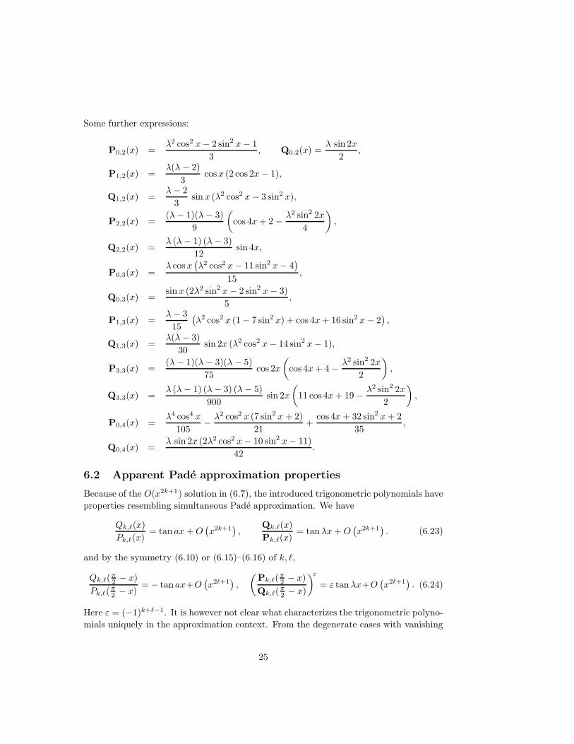
Some further expressions:

P0,2(x) =λ2 cos2 x− 2 sin2 x− 1

3, Q0,2(x) =

λ sin 2x

2,

P1,2(x) =λ(λ− 2)

3cosx (2 cos 2x− 1),

Q1,2(x) =λ− 2

3sinx (λ2 cos2 x− 3 sin2 x),

P2,2(x) =(λ− 1)(λ− 3)

9

(

cos 4x+ 2− λ2 sin2 2x

4

)

,

Q2,2(x) =λ (λ− 1) (λ− 3)

12sin 4x,

P0,3(x) =λ cosx

(

λ2 cos2 x− 11 sin2 x− 4)

15,

Q0,3(x) =sinx (2λ2 sin2 x− 2 sin2 x− 3)

5,

P1,3(x) =λ− 3

15

(

λ2 cos2 x (1− 7 sin2 x) + cos 4x+ 16 sin2 x− 2)

,

Q1,3(x) =λ(λ− 3)

30sin 2x (λ2 cos2 x− 14 sin2 x− 1),

P3,3(x) =(λ− 1)(λ− 3)(λ− 5)

75cos 2x

(

cos 4x+ 4− λ2 sin2 2x

2

)

,

Q3,3(x) =λ (λ− 1) (λ− 3) (λ− 5)

900sin 2x

(

11 cos 4x+ 19− λ2 sin2 2x

2

)

,

P0,4(x) =λ4 cos4 x

105− λ2 cos2 x (7 sin2 x+ 2)

21+

cos 4x+ 32 sin2 x+ 2

35,

Q0,4(x) =λ sin 2x (2λ2 cos2 x− 10 sin2 x− 11)

42.

6.2 Apparent Pade approximation properties

Because of the O(x2k+1) solution in (6.7), the introduced trigonometric polynomials have

properties resembling simultaneous Pade approximation. We have

Qk,ℓ(x)

Pk,ℓ(x)= tan ax+O

(

x2k+1)

,Qk,ℓ(x)

Pk,ℓ(x)= tanλx +O

(

x2k+1)

. (6.23)

and by the symmetry (6.10) or (6.15)–(6.16) of k, ℓ,

Qk,ℓ(π2− x)

Pk,ℓ(π2− x) = − tanax+O

(

x2ℓ+1)

,

(

Pk,ℓ(π2− x)

Qk,ℓ(π2− x)

)ε

= ε tanλx+O(

x2ℓ+1)

. (6.24)

Here ε = (−1)k+ℓ−1. It is however not clear what characterizes the trigonometric polyno-

mials uniquely in the approximation context. From the degenerate cases with vanishing

25

Pochhammer factors on the right-hand sides of (6.6) or (6.7) we get the following van-

ishing or exact approximation properties:

Pk,ℓ(x) = 0, Qk,ℓ(x) = 0, if (5.6) holds,

Qk,ℓ(x)

Pk,ℓ(x)= tan ax, if (5.8) holds,

Pk,ℓ(x)

Qk,ℓ(x)= − tanax, if (5.10) holds, (6.25)

Pk,ℓ(x) = 0, Qk,ℓ(x) = 0, if (5.7) holds,

Qk,ℓ(x)

Pk,ℓ(x)= tanλx, if (5.9) holds,

Pk,ℓ(x)

Qk,ℓ(x)= − tanλx, if (5.11) holds,

and similarly with Pk,ℓ(π2−x), Qk,ℓ(

π2−x) or Pk,ℓ(

π2−x),Qk,ℓ(

π2−x). These conditions

do not determine the trigonometric polynomials uniquely either, because Pk,ℓ(x),Qk,ℓ(x)

are not the shifted a 7→ λ− k − ℓ versions of Pk,ℓ(x), Qk,ℓ(x).

6.3 Contiguous relations

Contiguous relations for the considered 2F1 functions translate into the following recur-

rence relations:

Pk,ℓ(x) =a+ 2k − 1

2k − 1sin2 xPk−1,ℓ(x) +

a+ 2ℓ− 1

2ℓ− 1cos2 xPk,ℓ−1(x), (6.26)

(a

2+ k + ℓ+ 1

)

Pk,ℓ(x) =

(

k +1

2

)

Pk+1,ℓ(x) +

(

ℓ+1

2

)

Pk,ℓ+1(x), (6.27)

(

ℓ+1

2

)

Pk,ℓ+1(x) =

(

ℓ+1

2+ (a+ k + ℓ) cos2 x

)

Pk,ℓ(x)

−a+ 2ℓ− 1

2ℓ− 1

( a

2+ k + ℓ

)

cos2 xPk,ℓ−1(x). (6.28)

The recurrence relations for Qk,ℓ’s are the same. Three-term recurrences for the trigono-

metric polynomials Pk,ℓ(x), Qk,ℓ(x) are less clear, because some shifts in k, ℓ lead to

half-integer shifts in the upper parameters of the 2F1 functions, and transformation (6.14)

mixes Pk,ℓ’s with Qk,ℓ’s. Since we formally have Q0,0(x) = 0, Q0,−1(x) = 0, three-term

recurrences between these polynomials with minimal shifts in k, ℓ should not be expected.

26

Here are some consequences of the contiguous relations, nevertheless:

(

2k cos2 x+ 2ℓ sin2 x+ 1)

Pk,ℓ(x) =2k + 1

2ℓ− 1(λ− k + ℓ− 1) cos2 xPk+1,ℓ−1(x)

+2ℓ+ 1

2k − 1(λ+ k − ℓ− 1) sin2 xPk−1,ℓ+1(x), (6.29)

sin2 x

2k + 1Pk,ℓ(x) +

Pk+1,ℓ+1(x)

λ− k − ℓ− 1=

λ− k + ℓ− 1

(2ℓ− 1)(2ℓ+ 1)cos2 xPk+1,ℓ−1(x), (6.30)

(2ℓ− 1)Pk,ℓ(x) =λ2 − (k + ℓ)2

(2k − 1)(2k + 1)(λ− k − ℓ+ 1) sin2 xPk−1,ℓ−1(x)

+(λ− k + ℓ − 1)Pk+1,ℓ−1(x). (6.31)

6.4 A hyperbolic trigonometric version of (3.1)

A trigonometric version of formula (3.1) is pointless, because the substitution z 7→ − tan2 x

does not give a meaningful 2F1 argument for a local expansion. We may however use the

hyperbolic tangent substitution z 7→ tanh2 x (plus a 7→ λ − k − ℓ for a little neatness),

and consider the approximation x→ +∞:

2F1

( λ−k−ℓ2

, λ−k+ℓ+1

2

λ+ 1

∣

∣

∣

∣

1

cosh2 x

)

= 2λ coshλ x (coshλx− sinhλx) tanhk x×

F3

(

k + 1, ℓ+ 1;−k,−ℓλ+ 1

∣

∣

∣

∣

1− cothx

2,1− tanhx

2

)

. (6.32)

Trigonometric expressions for the dihedral functions with kℓ = 0 or k = ℓ could be

obtained in relation to the Legendre functions (as described in Remark 4.2). Infinite

trigonometric series for general Legendre functions are given in [1, 8.7.1–8.7.2].

6.5 Trigonometric expressions for logarithmic solutions

The use of trigonometric arguments is instructive for degenerate or logarithmic dihedral

2F1 functions as well, as suggested by formulas (1.4), (1.5). In the logarithmic cases (5.8),

(5.10) the non-logarithmic solution like (5.14) in (3.2) or (3.3) is, respectively,

Pk,ℓ(x)

cos ax, −Qk,ℓ(x)

cos ax, (6.33)

due to (6.25). The logarithmic solution is obtained by differentiating (6.9) or (6.8) with

respect to a. Under condition (5.8), the left hand side of (5.19) if a is even, or (5.20) if

a is odd, is equal to

xPk,ℓ(x)

cos ax+dPk,ℓ(x)

dasin ax− dQk,ℓ(x)

dacos ax, with a = −m. (6.34)

Under condition (5.10), the left hand side of (5.21) is equal to

xQk,ℓ(x)

cos ax+dPk,ℓ(x)

dacos ax+

dQk,ℓ(x)

dasin ax, with a = −m. (6.35)

27

Similar expressions can be obtained with the more compact trigonometric polynomials

Pk,ℓ(x),Qk,ℓ(x), which depend on the parameter λ = a+ k + ℓ.

References

[1] M. Abramowitz and I.A. Stegun. Handbook of mathematical functions, with formu-

las, graphs and mathematical tables. Number 55 in Applied Math. Series. Nat. Bur.

Standards, Washington, D.C., 1964.

[2] G.E. Andrews, R. Askey, and R. Roy. Special Functions. Cambridge Univ. Press,

Cambridge, 1999.

[3] F. Beukers. Gauss’ hypergeometric function. In W. Abikoff et al, editor, The

Mathematical Legacy of Wilhelm Magnus: Groups, geometry and special functions,

volume 169 of Contemporary Mathematics series, pages 29–43. AMS, Providence,

2007.

[4] A. Erdelyi, editor. Higher Transcendental Functions, volume I. McGraw-Hill Book

Company, New-York, 1953.

[5] M. Petkovsek, H.S. Wilf, and D. Zeilberger. A=B. A. K. Peters, Wellesley, Mas-

sachusetts, 1996.

[6] H. M. Srivastava and P. W. Karlsson. Multiple Gaussian Hypergeometric Series.

Ellis Horwood Ltd., 1985.

[7] R. Vidunas. Degenerate Gauss hypergeometric functions. Kyushu Journal of Math-

ematics, 61:109–135, 2007. Available at http://arxiv.org/math.CA/0407265.

[8] R. Vidunas. Algebraic transformations of Gauss hypergeometric

functions. Funkcialaj Ekvacioj, 52(2):139–180, 2009. Available at

http://arxiv.org/math.CA/0408269.

[9] R. Vidunas. Specialization of Appell’s functions to univariate hypergeometric func-

tions. Journal of Mathematical Analysis and Applications, 355:145–163, 2009. Avail-

able at http://arxiv.org/abs/0804.0655.

[10] R. Vidunas. Transformations and invariants for dihedral Gauss hypergeometric

functions. Available at http://arxiv.org/abs/1101.3688., 2011.

[11] Wikipedia. Hypergeometric series. http://en.wikipedia.org/wiki/Hypergeometric series.

28