Diophantine approximations for a constant related to elliptic functions

J. Math. Soc. JapanVol. 53, No. 4, 2001

Diophantine approximations for a constant related to elliptic

functions

By Marc Huttner and Tapani Matala-aho

(Received Jun. 5, 2000)

Abstract. This paper is devoted to the study of rational approximations of the

ratio h�l�=o�l�, where o�l� and h�l� are the real period and real quasi-period, re-

spectively, of the elliptic curve y2 � x�xÿ 1��xÿ l�. Using monodromy principle for

hypergeometric function in the logarithm case we obtain rational approximations of

�h=o��l� with l A Q and we shall ®nd new measures of irrationality, both in the

archimedean and non archimedean case.

1. Results and notations.

The Gauss hypergeometric function is de®ned by the power series

2F1a; b

c

�

�

�

�

x

� �

�X

y

n�0

�a�n�b�n�c�nn!

xn; �c0 0;ÿ1;ÿ2; . . .�;�1�

where �a�0 � 1 and �a�n � a�a� 1��a� 2� � � � �a� nÿ 1� for nb 1.

This series is an analytic solution in jxj < 1 to the diërential equation.

x�1ÿ x�y 00 � �cÿ �a� b� 1�x�y 0 ÿ aby � 0�2�

Let El be the family of elliptic curves

y2 � x�xÿ 1��xÿ l��3�

where l A C �, 0 < jlj < 1. Legendre notations for the periods of these curves

(i.e. complete integrals of the ®rst kind) and quasi-period (i.e. complete integrals

of the second kind) are, respectively

o�l� �def p

22F1

1=2; 1=2

1

�

�

�

�

l

� �

�4�

2000 Mathematics Subject Classi®cation. 11J82, 33C75, 34A20, 11J61.

Key Words and Phrase. Measure of irrationality, Elliptic integrals, hypergeometric function,

Diërential equations in the complex domain, p-adic.

h�l� �def p22F1

ÿ1=2; 1=2

1

�

�

�

�

l

� �

�5�

G�l� � h�l�=o�l�:�6�

There is no loss of generality in studying the diophantine approximations of

2F13=2; 3=2

2

�

�

�

�

l

� ��

2F11=2; 1=2

1

�

�

�

�

l

� �

:�7�

Indeed, from the contiguous relation, we have

2F13=2; 3=2

2

�

�

�

�

l

� ��

2F11=2; 1=2

1

�

�

�

�

l

� �

� 1

l�1ÿ l� �G�l� � lÿ 1�;�8�

so we can study equivalently the fraction (7).

We shall denote by Qp the p-adic completion of Q, where p A fy,

primes pg, in particular Qy

� R. For an irrational number y A Qp, we shall call

the irrationality measure mp�y� of y the in®mum of the m's satisfying the fol-

lowing condition: for any e > 0 there exists an H0 � H0�e� such that

jaÿ P=Qjp > Hÿmÿe

for any rational P=Q satisfying H � maxfjPj; jQjgbH0. From now on we

denote my�y� � m�y�. All our measures are eëctive in the sense that H0 can be

eëctively determined. Throughout this paper, we also suppose that l is a

rational number, p a prime number and vp�l� � v the p-adic valuation of l � pv �a=b, a A Z; b A Z�, pa ab and we set jljp � pÿv. We also use the notation

u�a� � 2v2�a�; if v2�a� < 4

24; if v2�a�b 4

�

In the following theorems let a=b A Q� be such that �a; b� � 1 and b A Z�.In the archimedean case we have

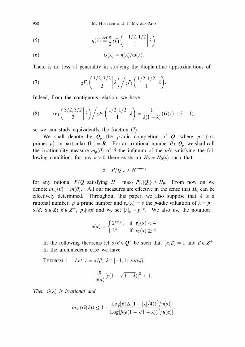
Theorem 1. Let l � a=b, l A �ÿ1; 1� satisfy

b

u�a� �e�1ÿ��

1ÿ lp

��2 < 1:

Then G�l� is irrational and

my�G�l��a 1ÿ Log�b�2e�1� jlj=4��2=u�a��Log�b�e�1ÿ

��

1ÿ lp

��2=u�a��:

M. Huttner and T. Matala-Aho958

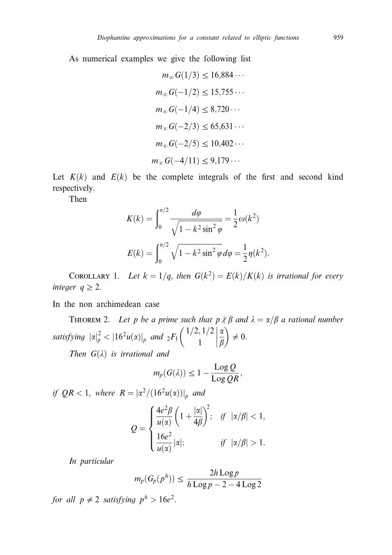
As numerical examples we give the following list

myG�1=3�a 16;884 � � �

myG�ÿ1=2�a 15;755 � � �

myG�ÿ1=4�a 8;720 � � �

myG�ÿ2=3�a 65;631 � � �

myG�ÿ2=5�a 10;402 � � �

myG�ÿ4=11�a 9;179 � � �

Let K�k� and E�k� be the complete integrals of the ®rst and second kind

respectively.

Then

K�k� �

� p=2

0

dj��

1ÿ k2 sin2 j

q �1

2o�k2�

E�k� �

� p=2

0

��

1ÿ k2 sin2 j

q

dj �1

2h�k2�:

Corollary 1. Let k � 1=q, then G�k2� � E�k�=K�k� is irrational for every

integer qb 2.

In the non archimedean case

Theorem 2. Let p be a prime such that pa b and l � a=b a rational number

satisfying jaj2p < j162u�a�jp and 2F1

1=2; 1=2

1

�

�

�

�

a

b

� �

0 0.

Then G�l� is irrational and

mp�G�l��a 1ÿLogQ

LogQR;

if QR < 1, where R � ja2=�162u�a��jp and

Q �

4e2b

u�a�1�

jaj

4b

� �2

; if ja=bj < 1,

16e2

u�a�jaj; if ja=bj > 1.

8

>

>

>

<

>

>

>

:

In particular

mp�Gp�ph��a

2hLog p

hLog pÿ 2ÿ 4Log 2

for all p0 2 satisfying ph > 16e2.

Diophantine approximations for a constant related to elliptic functions 959

2. Derivation of the approximation form.

Let nb 1 be an integer. We want to ®nd a remainder function Rn�x� such

that ord0 Rnb 2n and

Rn�x� � Pn�x�2F1a� 1; b� 1

c� 1

�

�

�

�

x

� �

ÿQnÿ1�x�2F1a; b

c

�

�

�

�

x

� �

�9�

for some polynomials Pn�x� and Qnÿ1�x� of degree n and nÿ 1, respectively.

Lemma 1. With the above notations

Rn�x� � Cnx2n

2F1a� n� 1; b� n� 1

c� 2n� 1

�

�

�

�

x

� �

where Cn 0 0 depends only on a; b; c and n.

Proof. Let us recall the main ideas of the Riemann's proof. Linear al-

gebra ensures us of the existence of two non zero polynomials Pn�x� and Qnÿ1�x�

of degree at most n and nÿ 1 respectively such that the linear form (11) satis®es

ord0 R�x�b 2n. The remainder function Rn�x� is an holomorphic solution in a

neighborhood of zero of a family of Fuchsian second order linear diërential

equation (2).

The non apparent singularities of (2) in P1�C� are 0; 1;y. We have to ®nd

the roots of indicial equations of (2) (Exponents of (2)). There is no loss of

generality in assuming that a; b and c are real.

In ``0'', lower bounds modN , for exponents are �2n;ÿc�.

In ``1'': �0; cÿ aÿ bÿ 1�.

In ``y'': (Using local parameter t � 1=x), �ÿn� a� 1;ÿn� b� 1�.

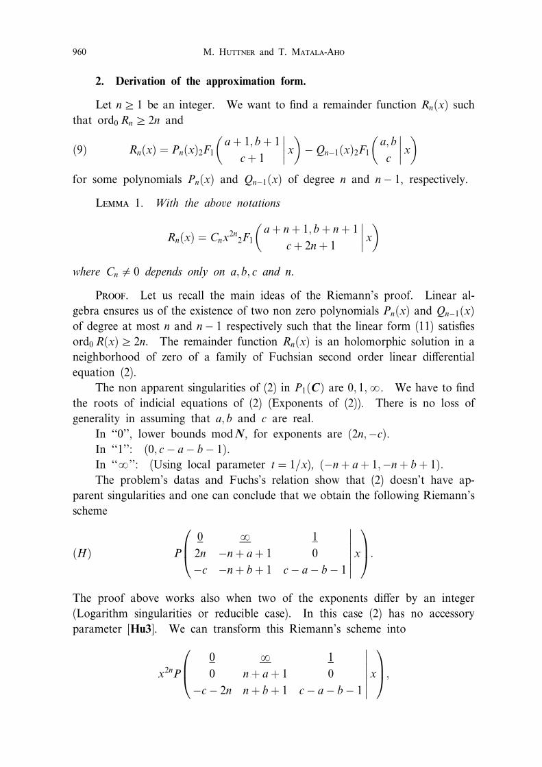
The problem's datas and Fuchs's relation show that (2) doesn't have ap-

parent singularities and one can conclude that we obtain the following Riemann's

scheme

P

0 y 1

2n ÿn� a� 1 0

ÿc ÿn� b� 1 cÿ aÿ bÿ 1

�

�

�

�

�

�

�

x

0

B

@

1

C

A:�H�

The proof above works also when two of the exponents diër by an integer

(Logarithm singularities or reducible case). In this case (2) has no accessory

parameter [Hu3]. We can transform this Riemann's scheme into

x2nP

0 y 1

0 n� a� 1 0

ÿcÿ 2n n� b� 1 cÿ aÿ bÿ 1

�

�

�

�

�

�

�

x

0

B

@

1

C

A;


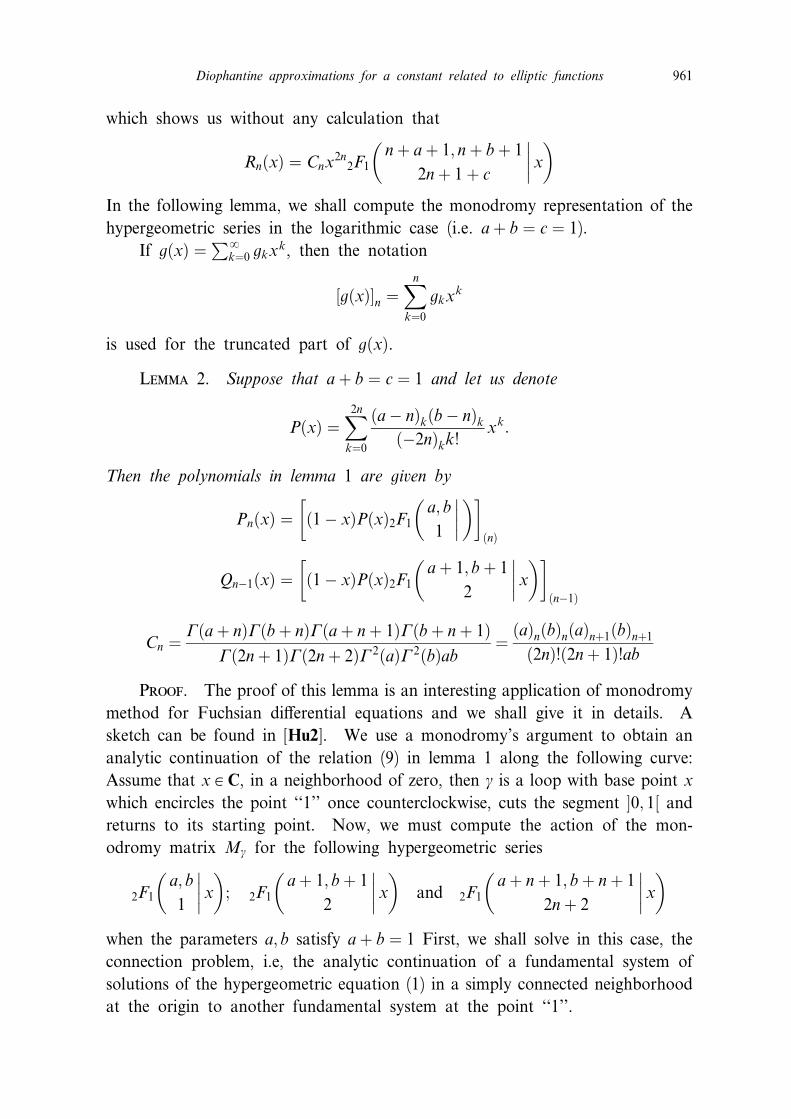
which shows us without any calculation that

Rn�x� � Cnx2n

2F1n� a� 1; n� b� 1

2n� 1� c

�

�

�

�

x

� �

In the following lemma, we shall compute the monodromy representation of the

hypergeometric series in the logarithmic case (i.e. a� b � c � 1).

If g�x� �P

y

k�0 gkxk, then the notation

�g�x��n �X

n

k�0

gkxk

is used for the truncated part of g�x�.

Lemma 2. Suppose that a� b � c � 1 and let us denote

P�x� �X

2n

k�0

�aÿ n�k�bÿ n�k�ÿ2n�kk!

xk:

Then the polynomials in lemma 1 are given by

Pn�x� � �1ÿ x�P�x�2F1a; b

1

�

�

�

�

� ��

�n�

Qnÿ1�x� � �1ÿ x�P�x�2F1a� 1; b� 1

2

�

�

�

�

x

� ��

�nÿ1�

Cn �G�a� n�G�b� n�G�a� n� 1�G�b� n� 1�

G�2n� 1�G�2n� 2�G 2�a�G 2�b�ab�

�a�n�b�n�a�n�1�b�n�1

�2n�!�2n� 1�!ab

Proof. The proof of this lemma is an interesting application of monodromy

method for Fuchsian diërential equations and we shall give it in details. A

sketch can be found in [Hu2]. We use a monodromy's argument to obtain an

analytic continuation of the relation (9) in lemma 1 along the following curve:

Assume that x A C, in a neighborhood of zero, then g is a loop with base point x

which encircles the point ``1'' once counterclockwise, cuts the segment �0; 1� and

returns to its starting point. Now, we must compute the action of the mon-

odromy matrix Mg for the following hypergeometric series

2F1a; b

1

�

�

�

�

x

� �

; 2F1a� 1; b� 1

2

�

�

�

�

x

� �

and 2F1a� n� 1; b� n� 1

2n� 2

�

�

�

�

x

� �

when the parameters a; b satisfy a� b � 1 First, we shall solve in this case, the

connection problem, i.e, the analytic continuation of a fundamental system of

solutions of the hypergeometric equation (1) in a simply connected neighborhood

at the origin to another fundamental system at the point ``1''.


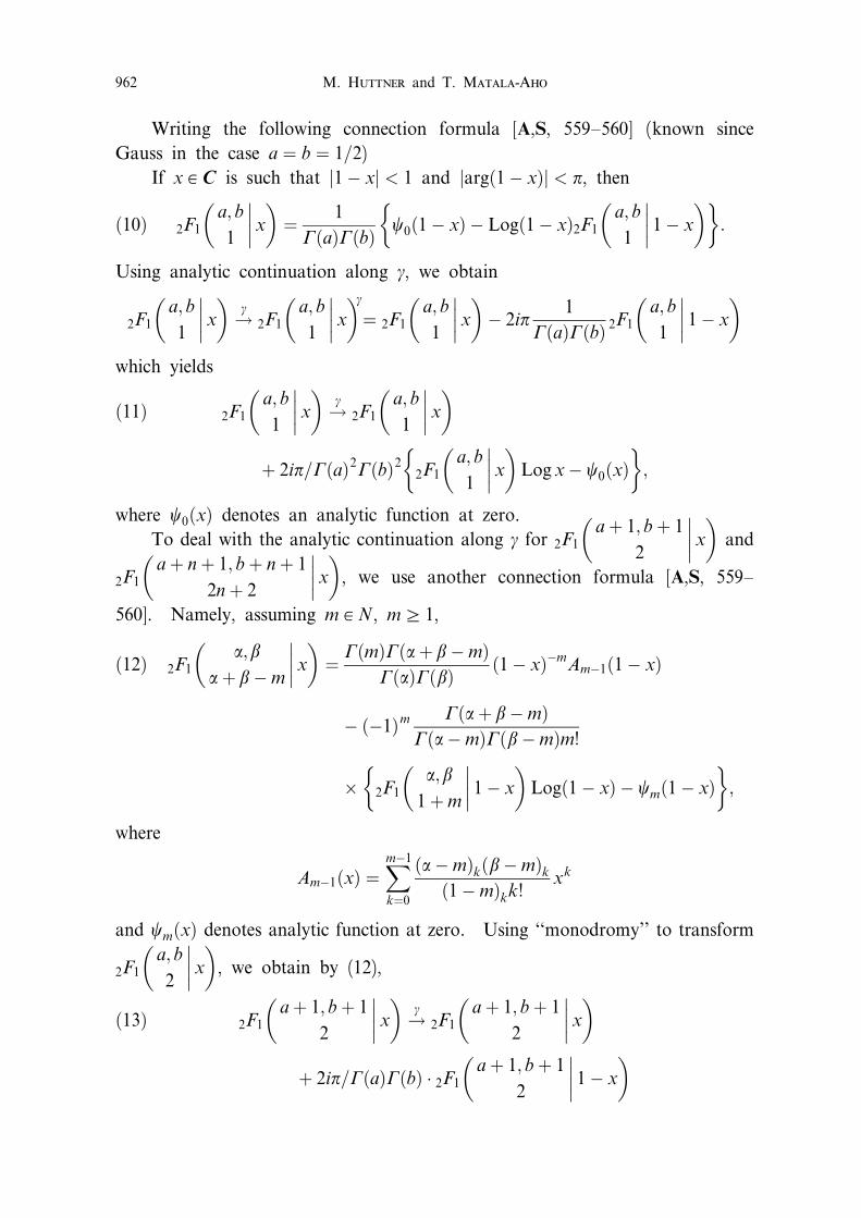
Writing the following connection formula [A,S, 559±560] (known since

Gauss in the case a � b � 1=2)

If x A C is such that j1ÿ xj < 1 and jarg�1ÿ x�j < p, then

2F1a; b

1

�

�

�

�

x

� �

�1

G�a�G�b�c0�1ÿ x� ÿ Log�1ÿ x�2F1

a; b

1

�

�

�

�

1ÿ x

� ��

:�10�

Using analytic continuation along g, we obtain

2F1a; b

1

�

�

�

�

x

� �

!g

2F1a; b

1

�

�

�

�

x

� �g

� 2F1a; b

1

�

�

�

�

x

� �

ÿ 2ip1

G�a�G�b�2F1

a; b

1

�

�

�

�

1ÿ x

� �

which yields

2F1a; b

1

�

�

�

�

x

� �

!g

2F1a; b

1

�

�

�

�

x

� �

�11�

� 2ip=G�a�2G�b�2 2F1a; b

1

�

�

�

�

x

� �

Log xÿ c0�x�

� �

;

where c0�x� denotes an analytic function at zero.

To deal with the analytic continuation along g for 2F1a� 1; b� 1

2

�

�

�

�

x

� �

and

2F1a� n� 1; b� n� 1

2n� 2

�

�

�

�

x

� �

, we use another connection formula [A,S, 559±

560]. Namely, assuming m A N, mb 1,

2F1a; b

a� b ÿm

�

�

�

�

x

� �

�G�m�G�a� b ÿm�

G�a�G�b��1ÿ x�ÿm

Amÿ1�1ÿ x��12�

ÿ �ÿ1�mG�a� b ÿm�

G�aÿm�G�b ÿm�m!

� 2F1a; b

1�m

�

�

�

�

1ÿ x

� �

Log�1ÿ x� ÿ cm�1ÿ x�

� �

;

where

Amÿ1�x� �X

mÿ1

k�0

�aÿm�k�b ÿm�

k

�1ÿm�kk!

xk

and cm�x� denotes analytic function at zero. Using ``monodromy'' to transform

2F1a; b

2

�

�

�

�

x

� �

, we obtain by (12),

2F1a� 1; b� 1

2

�

�

�

�

x

� �

!g

2F1a� 1; b� 1

2

�

�

�

�

x

� �

�13�

� 2ip=G�a�G�b� � 2F1a� 1; b� 1

2

�

�

�

�

1ÿ x

� �


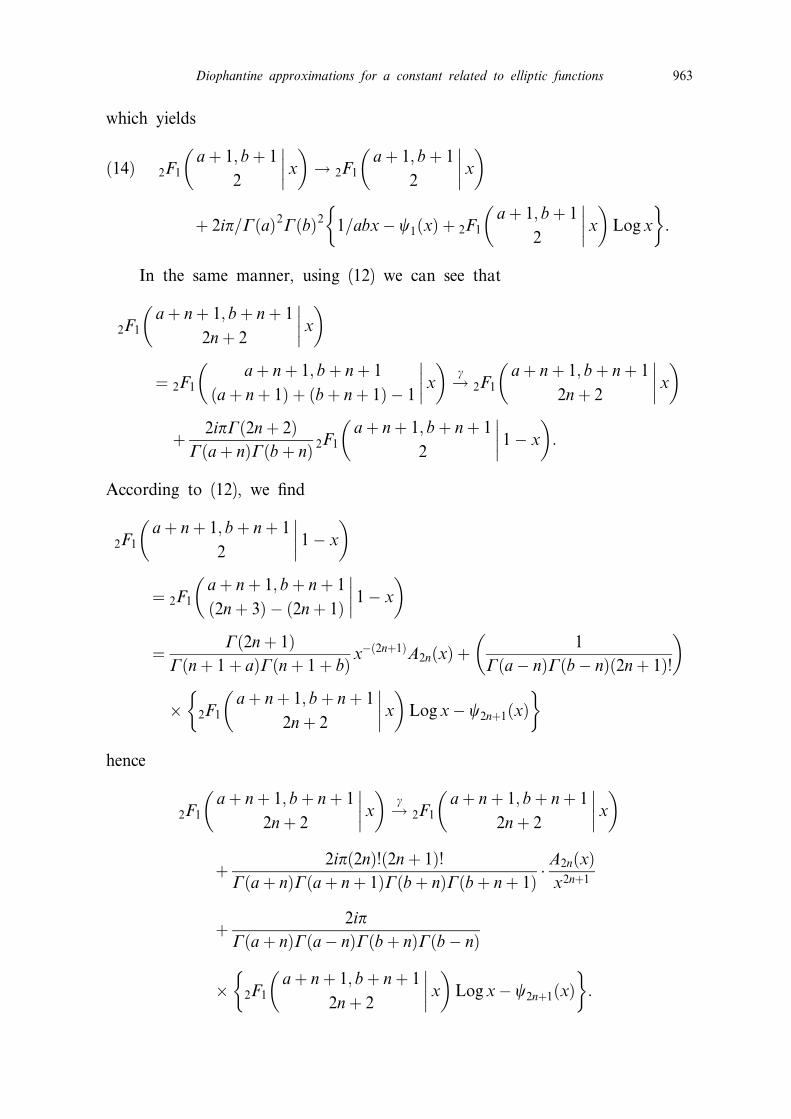
which yields

2F1a� 1; b� 1

2

�

�

�

�

x

� �

! 2F1a� 1; b� 1

2

�

�

�

�

x

� �

�14�

� 2ip=G�a�2G�b�2�

1=abxÿ c1�x� � 2F1a� 1; b� 1

2

�

�

�

�

x

� �

Log x

�

:

In the same manner, using (12) we can see that

2F1a� n� 1; b� n� 1

2n� 2

�

�

�

�

x

� �

� 2F1a� n� 1; b� n� 1

�a� n� 1� � �b� n� 1� ÿ 1

�

�

�

�

x

� �

!g

2F1a� n� 1; b� n� 1

2n� 2

�

�

�

�

x

� �

�2ipG�2n� 2�

G�a� n�G�b� n�2F1

a� n� 1; b� n� 1

2

�

�

�

�

1ÿ x

� �

:

According to (12), we ®nd

2F1a� n� 1; b� n� 1

2

�

�

�

�

1ÿ x

� �

� 2F1a� n� 1; b� n� 1

�2n� 3� ÿ �2n� 1�

�

�

�

�

1ÿ x

� �

�G�2n� 1�

G�n� 1� a�G�n� 1� b�xÿ�2n�1�A2n�x� �

1

G�aÿ n�G�bÿ n��2n� 1�!

� �

� 2F1a� n� 1; b� n� 1

2n� 2

�

�

�

�

x

� �

Log xÿ c2n�1�x�

� �

hence

2F1a� n� 1; b� n� 1

2n� 2

�

�

�

�

x

� �

!g

2F1a� n� 1; b� n� 1

2n� 2

�

�

�

�

x

� �

�2ip�2n�!�2n� 1�!

G�a� n�G�a� n� 1�G�b� n�G�b� n� 1��A2n�x�

x2n�1

�2ip

G�a� n�G�aÿ n�G�b� n�G�bÿ n�

� 2F1a� n� 1; b� n� 1

2n� 2

�

�

�

�

x

� �

Log xÿ c2n�1�x�

� �

:


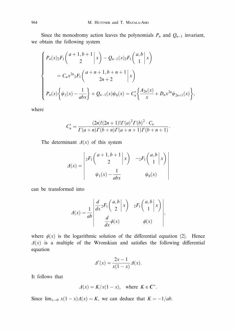
Since the monodromy action leaves the polynomials Pn and Qnÿ1 invariant,

we obtain the following system

Pn�x�2F1a� 1; b� 1

2

�

�

�

�

x

� �

ÿQnÿ1�x�2F1a; b

1

�

�

�

�

x

� �

� Cnx2n

2F1a� n� 1; b� n� 1

2n� 2

�

�

�

�

x

� �

Pn�x� c1�x� ÿ1

abx

� �

�Qnÿ1�x�c0�x� � C 0n

A2n�x�

x�Dnx

2nc2n�1�x�

� �

;

8

>

>

>

>

>

>

>

>

>

>

<

>

>

>

>

>

>

>

>

>

>

:

where

C 0n �

�2n�!�2n� 1�!G�a�2G�b�2 � Cn

G�a� n�G�b� n�G�a� n� 1�G�b� n� 1�:

The determinant D�x� of this system

D�x� �

�

�

�

�

�

�

�

�

�

2F1a� 1; b� 1

2

�

�

�

�

x

� �

ÿ2F1a; b

1

�

�

�

�

x

� �

c1�x� ÿ1

abxc0�x�

�

�

�

�

�

�

�

�

�

can be transformed into

D�x� �1

ab

�

�

�

�

�

�

�

�

�

d

dx2F1

a; b

2

�

�

�

�

x

� �

2F1a; b

1

�

�

�

�

x

� �

d

dxf�x� f�x�

�

�

�

�

�

�

�

�

�

;

where f�x� is the logarithmic solution of the diërential equation (2). Hence

D�x� is a multiple of the Wronskian and satis®es the following diërential

equation

D 0�x� �2xÿ 1

x�1ÿ x�D�x�:

It follows that

D�x� � K=x�1ÿ x�, where K A C�.

Since limx!0 x�1ÿ x�D�x� � K , we can deduce that K � ÿ1=ab.


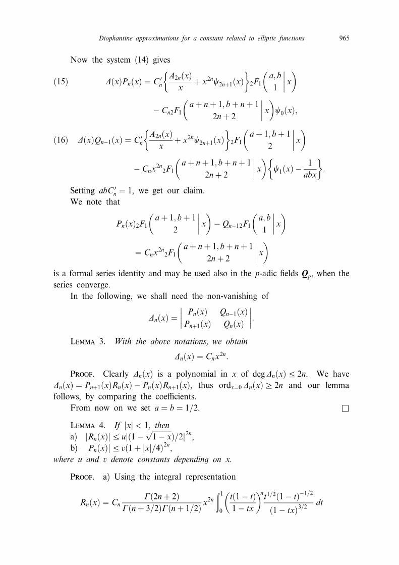
Now the system (14) gives

D�x�Pn�x� � C 0n

A2n�x�x

� x2nc2n�1�x��

2F1a; b

1

�

�

�

�

x

� �

�15�

ÿ Cn2F1a� n� 1; b� n� 1

2n� 2

�

�

�

�

x

� �

c0�x�;

D�x�Qnÿ1�x� � C 0n

A2n�x�x

� x2nc2n�1�x��

2F1a� 1; b� 1

2

�

�

�

�

x

� �

�16�

ÿ Cnx2n

2F1a� n� 1; b� n� 1

2n� 2

�

�

�

�

x

� �

c1�x� ÿ1

abx

� �

:

Setting abC 0n � 1, we get our claim.

We note that

Pn�x�2F1a� 1; b� 1

2

�

�

�

�

x

� �

ÿQnÿ12F1a; b

1

�

�

�

�

x

� �

� Cnx2n

2F1a� n� 1; b� n� 1

2n� 2

�

�

�

�

x

� �

is a formal series identity and may be used also in the p-adic ®elds Qp, when the

series converge.

In the following, we shall need the non-vanishing of

Dn�x� �Pn�x� Qnÿ1�x�Pn�1�x� Qn�x�

�

�

�

�

�

�

�

�

:

Lemma 3. With the above notations, we obtain

Dn�x� � Cnx2n.

Proof. Clearly Dn�x� is a polynomial in x of degDn�x�a 2n. We have

Dn�x� � Pn�1�x�Rn�x� ÿ Pn�x�Rn�1�x�, thus ordx�0 Dn�x�b 2n and our lemma

follows, by comparing the coe½cients.

From now on we set a � b � 1=2. r

Lemma 4. If jxj < 1, then

a) jRn�x�ja uj�1ÿ��

1ÿ xp

�=2j2n,b) jPn�x�ja v�1� jxj=4�2n,

where u and v denote constants depending on x.

Proof. a) Using the integral representation

Rn�x� � Cn

G�2n� 2�G�n� 3=2�G�n� 1=2� x

2n

�1

0

t�1ÿ t�1ÿ tx

� �nt1=2�1ÿ t�ÿ1=2

�1ÿ tx�3=2dt


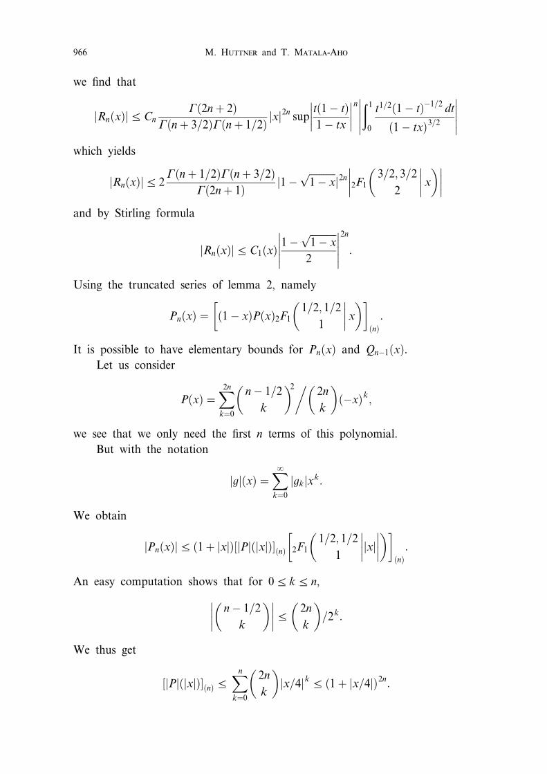
we ®nd that

jRn�x�jaCn

G�2n� 2�G�n� 3=2�G�n� 1=2� jxj

2nsup

t�1ÿ t�1ÿ tx

�

�

�

�

�

�

�

�

n �1

0

t1=2�1ÿ t�ÿ1=2dt

�1ÿ tx�3=2

�

�

�

�

�

�

�

�

�

�

which yields

jRn�x�ja 2G�n� 1=2�G�n� 3=2�

G�2n� 1� j1ÿ��

1ÿ xp

j2n 2F1

3=2; 3=2

2

�

�

�

�

x

� ��

�

�

�

�

�

�

�

and by Stirling formula

jRn�x�jaC1�x�1ÿ

��

1ÿ xp

2

�

�

�

�

�

�

�

�

�

�

2n

:

Using the truncated series of lemma 2, namely

Pn�x� � �1ÿ x�P�x�2F1

1=2; 1=2

1

�

�

�

�

x

� ��

�n�:

It is possible to have elementary bounds for Pn�x� and Qnÿ1�x�.Let us consider

P�x� �X

2n

k�0

nÿ 1=2

k

� �2�2n

k

� �

�ÿx�k;

we see that we only need the ®rst n terms of this polynomial.

But with the notation

jgj�x� �X

y

k�0

jgkjxk:

We obtain

jPn�x�ja �1� jxj��jPj�jxj��n� 2F1

1=2; 1=2

1

�

�

�

�

jxj�

�

�

�

� ��

�n�:

An easy computation shows that for 0a ka n,

nÿ 1=2

k

� ��

�

�

�

�

�

�

�

a2n

k

� �

=2k:

We thus get

�jPj�jxj��n�aX

n

k�0

2n

k

� �

jx=4jka �1� jx=4j�2n:


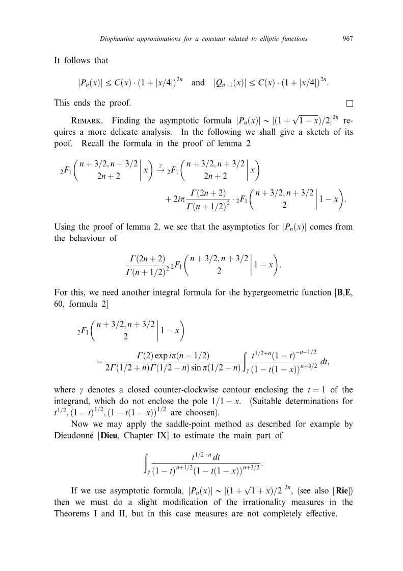
It follows that

jPn�x�jaC�x� � �1� jx=4j�2n and jQnÿ1�x�jaC�x� � �1� jx=4j�2n:

This ends the proof. r

Remark. Finding the asymptotic formula jPn�x�j@ j�1��

1ÿ xp

�=2j2n re-

quires a more delicate analysis. In the following we shall give a sketch of its

poof. Recall the formula in the proof of lemma 2

2F1n� 3=2; n� 3=2

2n� 2

�

�

�

�

x

� �

!g 2F1n� 3=2; n� 3=2

2n� 2

�

�

�

�

x

� �

� 2ipG�2n� 2�G�n� 1=2�2

� 2F1n� 3=2; n� 3=2

2

�

�

�

�

1ÿ x

� �

:

Using the proof of lemma 2, we see that the asymptotics for jPn�x�j comes from

the behaviour of

G�2n� 2�G�n� 1=2�2 2F1

n� 3=2; n� 3=2

2

�

�

�

�

1ÿ x

� �

:

For this, we need another integral formula for the hypergeometric function [B,E,

60, formula 2]

2F1n� 3=2; n� 3=2

2

�

�

�

�

1ÿ x

� �

� G�2� exp ip�nÿ 1=2�2G�1=2� n�G�1=2ÿ n� sin p�1=2ÿ n�

�

g

t1=2�n�1ÿ t�ÿnÿ1=2

�1ÿ t�1ÿ x��n�3=2dt;

where g denotes a closed counter-clockwise contour enclosing the t � 1 of the

integrand, which do not enclose the pole 1=1ÿ x. (Suitable determinations for

t1=2; �1ÿ t�1=2; �1ÿ t�1ÿ x��1=2 are choosen).

Now we may apply the saddle-point method as described for example by

DieudonneÂ [Dieu, Chapter IX] to estimate the main part of

�

g

t1=2�n dt

�1ÿ t�n�1=2�1ÿ t�1ÿ x��n�3=2:

If we use asymptotic formula, jPn�x�j@ j�1��

1� xp

�=2j2n, (see also [Rie])

then we must do a slight modi®cation of the irrationality measures in the

Theorems I and II, but in this case measures are not completely eëctive.


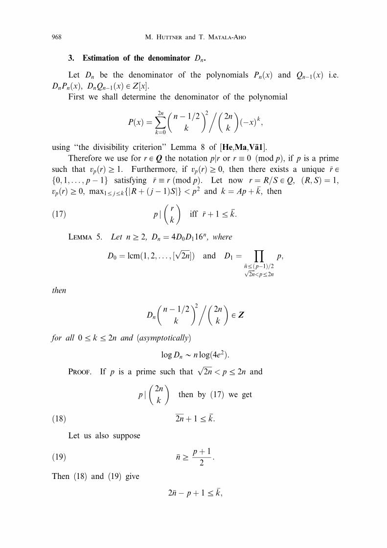
3. Estimation of the denominator Dn.

Let Dn be the denominator of the polynomials Pn�x� and Qnÿ1�x� i.e.

DnPn�x�, DnQnÿ1�x� A Z�x�.First we shall determine the denominator of the polynomial

P�x� �X

2n

k�0

nÿ 1=2

k

� �2� 2n

k

� �

�ÿx�k;

using ``the divisibility criterion'' Lemma 8 of [He,Ma,VaÈ1].

Therefore we use for r A Q the notation pjr or r1 0 �mod p�, if p is a prime

such that vp�r�b 1. Furthermore, if vp�r�b 0, then there exists a unique r A

f0; 1; . . . ; pÿ 1g satisfying r1 r �mod p�. Let now r � R=S A Q, �R;S� � 1,

vp�r�b 0, max1a jakfjR� � j ÿ 1�Sjg < p2 and k � Ap� k, then

p j r

k

� �

iff r� 1a k:�17�

Lemma 5. Let nb 2, Dn � 4D0D116n, where

D0 � lcm�1; 2; . . . ; ��

2np

�� and D1 �Y

na�pÿ1�=2��

2np

<pa2n

p;

then

Dn

nÿ 1=2

k

� �2� 2n

k

� �

A Z

for all 0a ka 2n and (asymptotically)

logDn @ n log�4e2�.

Proof. If p is a prime such that��

2np

< pa 2n and

p j 2n

k

� �

then by �17� we get

2n� 1a k:�18�

Let us also suppose

nbp� 1

2:�19�

Then (18) and (19) give

2nÿ p� 1a k;


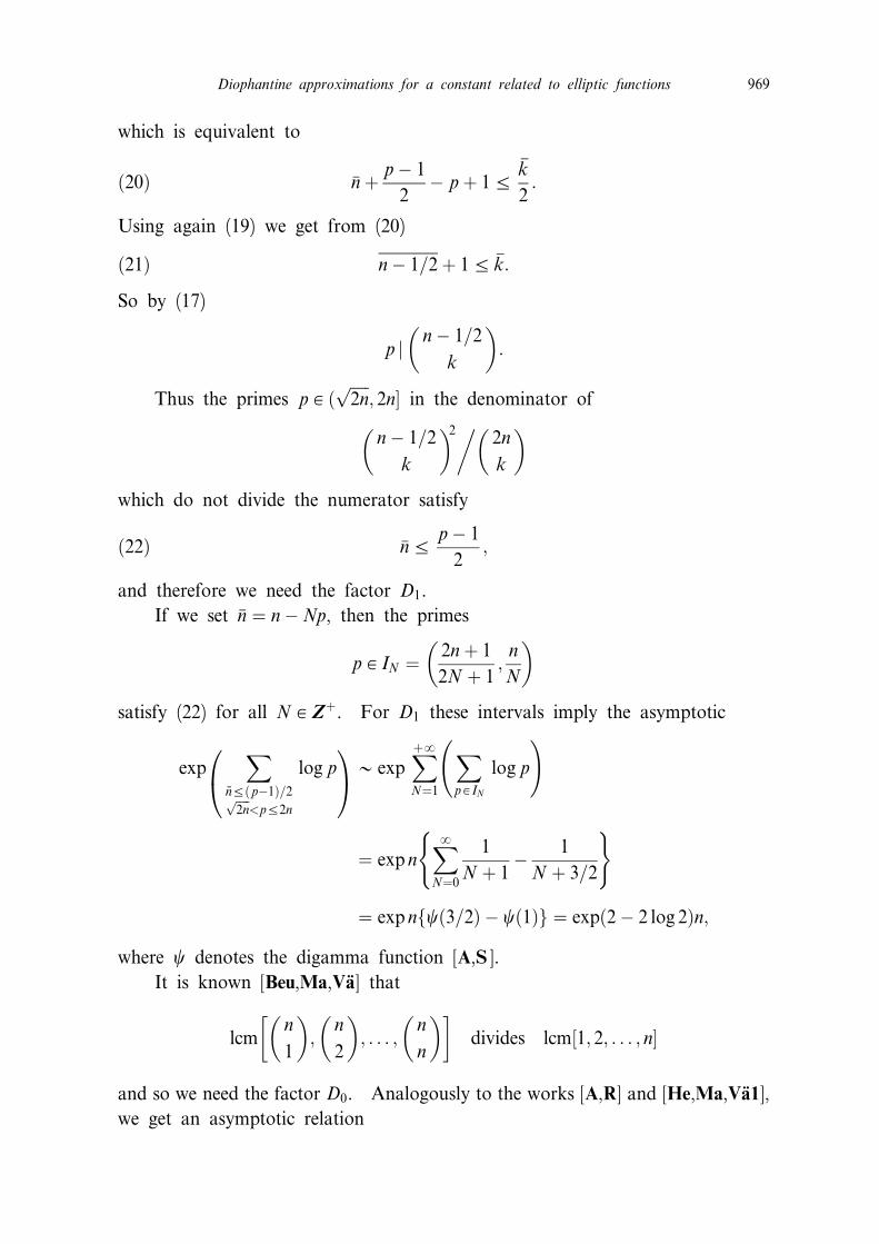
which is equivalent to

n� pÿ 1

2ÿ p� 1a

k

2:�20�

Using again (19) we get from (20)

nÿ 1=2� 1a k:�21�

So by (17)

p j nÿ 1=2

k

� �

:

Thus the primes p A ��

2np

; 2n� in the denominator of

nÿ 1=2

k

� �2� 2n

k

� �

which do not divide the numerator satisfy

napÿ 1

2;�22�

and therefore we need the factor D1.

If we set n � nÿNp, then the primes

p A IN � 2n� 1

2N � 1;n

N

� �

satisfy (22) for all N A Z�. For D1 these intervals imply the asymptotic

exp0

@

X

na�pÿ1�=2��

2np

<pa2n

log p

1

A

@ expX

�y

N�1

X

p A IN

log p

!

� exp nX

y

N�0

1

N � 1ÿ 1

N � 3=2

( )

� exp nfc�3=2� ÿ c�1�g � exp�2ÿ 2 log 2�n;

where c denotes the digamma function [A,S ].

It is known [Beu,Ma,VaÈ ] that

lcmn

1

� �

;n

2

� �

; . . . ;n

n

� ��

divides lcm�1; 2; . . . ; n�

and so we need the factor D0. Analogously to the works [A,R] and [He,Ma,VaÈ1],

we get an asymptotic relation


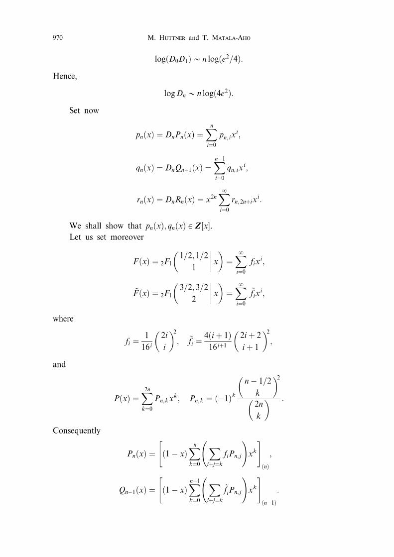
log�D0D1�@ n log�e2=4�.

Hence,

logDn @ n log�4e2�.

Set now

pn�x� � DnPn�x� �X

n

i�0

pn; ixi;

qn�x� � DnQnÿ1�x� �X

nÿ1

i�0

qn; ixi;

rn�x� � DnRn�x� � x2nX

y

i�0

rn;2n�ixi:

We shall show that pn�x�; qn�x� A Z�x�.

Let us set moreover

F �x� � 2F1

1=2; 1=2

1

�

�

�

�

x

� �

�X

y

i�0

fixi;

~F �x� � 2F1

3=2; 3=2

2

�

�

�

�

x

� �

�X

y

i�0

~fixi;

where

fi �1

16 i

2i

i

� �2

; ~fi �4�i � 1�

16 i�1

2i � 2

i � 1

� �2

;

and

P�x� �X

2n

k�0

Pn;kxk; Pn;k � �ÿ1�k

nÿ 1=2

k

� �2

2n

k

� � :

Consequently

Pn�x� � �1ÿ x�X

n

k�0

X

i�j�k

fiPn; j

!

xk

" #

�n�

;

Qnÿ1�x� � �1ÿ x�X

nÿ1

k�0

X

i�j�k

~fiPn; j

!

xk

" #

�nÿ1�

:


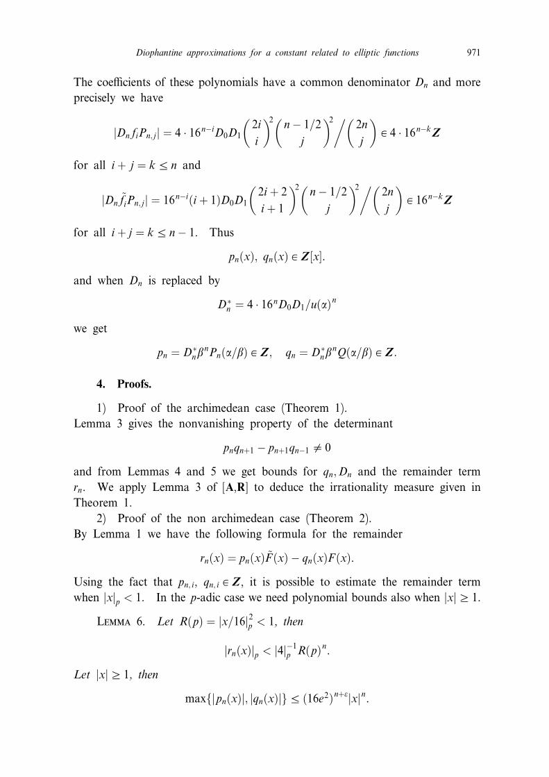
The coe½cients of these polynomials have a common denominator Dn and more

precisely we have

jDn fiPn; jj � 4 � 16nÿiD0D12i

i

� �2nÿ 1=2

j

� �2� 2n

j

� �

A 4 � 16nÿkZ

for all i � j � ka n and

jDn~fiPn; jj � 16nÿi�i � 1�D0D1

2i � 2

i � 1

� �2nÿ 1=2

j

� �2� 2n

j

� �

A 16nÿkZ

for all i � j � ka nÿ 1. Thus

pn�x�; qn�x� A Z�x�.

and when Dn is replaced by

D�n � 4 � 16nD0D1=u�a�

n

we get

pn � D�nb

nPn�a=b� A Z; qn � D�nb

nQ�a=b� A Z:

4. Proofs.

1) Proof of the archimedean case (Theorem 1).

Lemma 3 gives the nonvanishing property of the determinant

pnqn�1 ÿ pn�1qnÿ1 0 0

and from Lemmas 4 and 5 we get bounds for qn;Dn and the remainder term

rn. We apply Lemma 3 of [A,R] to deduce the irrationality measure given in

Theorem 1.

2) Proof of the non archimedean case (Theorem 2).

By Lemma 1 we have the following formula for the remainder

rn�x� � pn�x� ~F�x� ÿ qn�x�F�x�.

Using the fact that pn; i, qn; i A Z, it is possible to estimate the remainder term

when jxjp < 1. In the p-adic case we need polynomial bounds also when jxjb 1.

Lemma 6. Let R�p� � jx=16j2p < 1, then

jrn�x�jp < j4jÿ1p R�p�n.

Let jxjb 1, then

maxfjpn�x�j; jqn�x�jga �16e2�n�ejxjn.


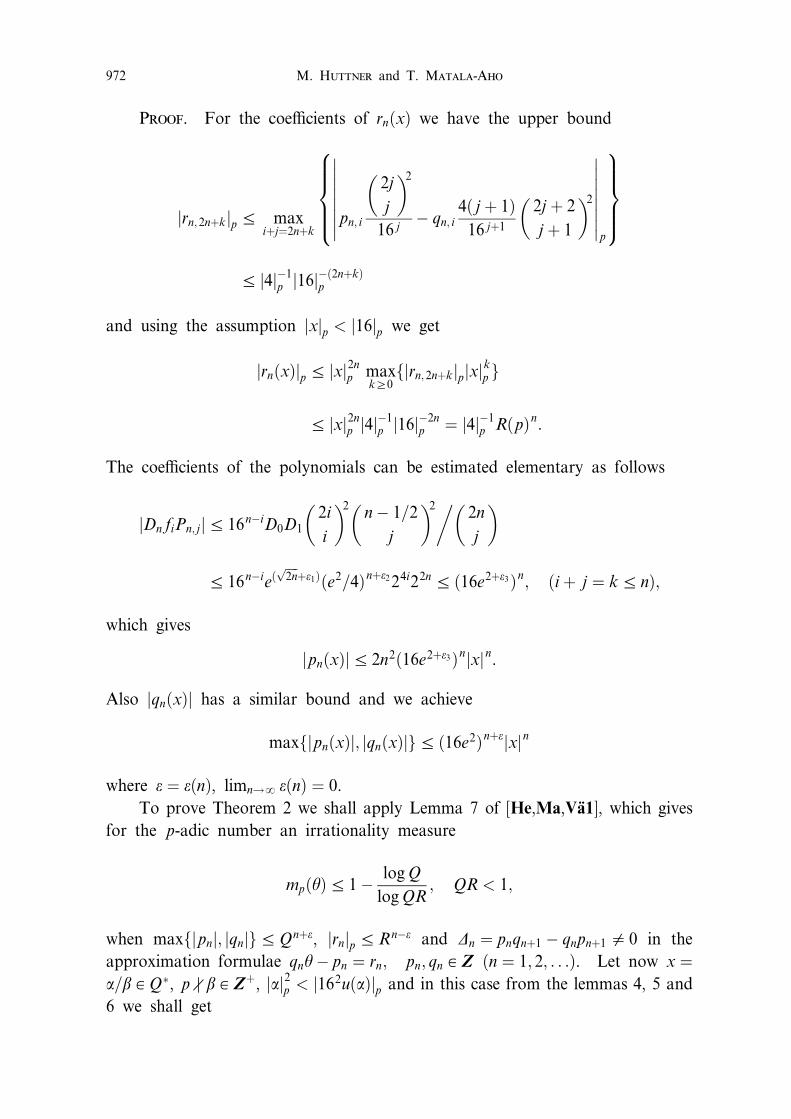
Proof. For the coe½cients of rn�x� we have the upper bound

jrn;2n�kjpa maxi�j�2n�k

8

>

>

>

<

>

>

>

:

�

�

�

�

�

�

�

�

pn; i

2j

j

� �2

16 jÿ qn; i

4� j � 1�16 j�1

2j � 2

j � 1

� �2

�

�

�

�

�

�

�

�

p

9

>

>

>

=

>

>

>

;

a j4jÿ1p j16jÿ�2n�k�

p

and using the assumption jxjp < j16jp we get

jrn�x�jpa jxj2np maxkb0

fjrn;2n�kjpjxjkp g

a jxj2np j4jÿ1p j16jÿ2n

p � j4jÿ1p R�p�n:

The coe½cients of the polynomials can be estimated elementary as follows

jDn fiPn; jja 16nÿiD0D12i

i

� �2nÿ 1=2

j

� �2� 2n

j

� �

a 16nÿie��

2np

�e1��e2=4�n�e224i22na �16e2�e3�n; �i � j � ka n�;

which gives

jpn�x�ja 2n2�16e2�e3�njxjn.

Also jqn�x�j has a similar bound and we achieve

maxfjpn�x�j; jqn�x�jga �16e2�n�ejxjn

where e � e�n�, limn!y e�n� � 0.

To prove Theorem 2 we shall apply Lemma 7 of [He,Ma,VaÈ1], which gives

for the p-adic number an irrationality measure

mp�y�a 1ÿ logQ

logQR; QR < 1;

when maxfjpnj; jqnjgaQn�e, jrnjpaRnÿe and Dn � pnqn�1 ÿ qnpn�1 0 0 in the

approximation formulae qnyÿ pn � rn; pn; qn A Z �n � 1; 2; . . .�. Let now x �a=b A Q�, pa b A Z

�, jaj2p < j162u�a�jp and in this case from the lemmas 4, 5 and

6 we shall get


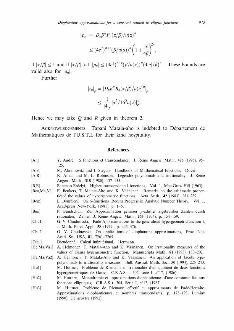
jpnj � jDnbnPn�a=b�=u�a�

nj

a �4e2�n�e�b=u�a��n 1�jaj

4b

� �2n

;

if ja=bja 1 and if ja=bj > 1 jpnja �4e2�n�e�b=u�a��n�4jaj=b�n. These bounds are

valid also for jqnj.

Further

jrnjp � jDnbnRn�a=b�=u�a�

njp

a1

j4jpja2=162u�a�jnp :

Hence we may take Q and R given in theorem 2.

Acknowledgements. Tapani Matala-aho is indebted to DeÂpartement de

MatheÂmatiques de l'U.S.T.L for their kind hospitality.

References

[An] Y. AndreÂ, G fonctions et transcendance, J. Reine Angew. Math., 476 (1996), 95±

125.

[A,S] M. Abramovitz and I. Stegun, Handbook of Mathematical functions, Dover.

[A,R] K. Alladi and M. L. Robinson, Legendre polynomials and irrationality, J. Reine

Angew. Math., 318 (1980), 137±155.

[B,E] Bateman-Erdelyi, Higher transcendantal fonctions, Vol. 1, Mac-Graw-Hill (1963).

[Beu,Ma,VaÈ] F. Beukers, T. Matala-Aho and K. VaÈaÈnaÈnen, Remarks on the arithmetic proper-

tiesof the values of hypergeometric functions, Acta Arith., 42 (1983), 281±289.

[Bom] E. Bombieri, On G-functions. Recent Progress in Analytic Number Theory, Vol. 1,

Acad-press New-York, (1981), p. 1±67.

[Bun] P. Bundschuh, Zur Approximation gewisser p-adisher algebraisher Zahlen durch

rationalen, Zahlen. J. Reine Angew. Math., 265 (1974), p. 154±159.

[Chu1] G. V. Chudnovski, PadeÂ Approximations to the generalised hypergeometricfunction I,

J. Math. Pures Appl., 58 (1979), p. 445±476.

[Chu2] G. V. Chudnovski, On applications of diophantine approximations, Proc. Nat.

Acad. Sci. USA, 81, 7261±7265.

[Dieu] DieudonneÂ, Calcul in®niteÂsimal, Hermann.

[He,Ma,VaÈ1] A. Heimonen, T. Matala-Aho and K. VaÈaÈnaÈnen, On irrationality measures of the

values of Gauss hypergeometric function, Manuscripta Math., 81 (1993), 183±202.

[He,Ma,VaÈ2] A. Heimonen, T. Matala-Aho and K. VaÈaÈnaÈnen, An application of Jacobi type-

polynomials to irrationality measures, Bull. Austral. Math. Soc., 50 (1994), 225±243.

[Hu1] M. Huttner, ProbleÁme de Riemann et irrationaliteÂ d'un quotient de deux fonctions

hypergeÂomeÂtriques de Gauss, C.R.A.S, t. 302, seÂrie I, n�17, (1986).

[Hu2] M. Huttner, Monodromie et approximations diophantiennes d'une constante lieÂe aux

fonctions elliptiques, C.R.A.S t. 304, SeÂrie I, n�12, (1987).

[Hu3] M. Huttner, ProbleÁme de Riemann eëctif et approximants de PadeÂ-Hermite.

Approximations diophantiennes et nombres transcendants, p. 173±193, Luminy

(1990), De gruyter (1992).


[Ma] W. Maier, Potenzreihen irrationalen grenzwertes, J. Reine Angew Math., 156

(1927), 93±148.

[Rie] B. Riemann, êuvres matheÂmatiques BlanchardÐParis, (1968).

[Sch] Th. Schneider, Introduction aux nombres transcendants, Gauthier-Villars, Paris,

(1959).

Marc Huttner

UFR de MatheÂmatiques

URA D751 au CNRS

UniversiteÂ de Lille I

F-59655ÐVilleneuve d'AscqÐFrance

Tapani Matala-aho

Matemaattisten tieteiden Laitos

PL 3000, 90014 Oulun Yliopisto

Finland


Documents

Diophantine approximations for a constant related to elliptic functions