Direct methods and protein crystallography at low resolution

Acta Cryst. (2000). D56, 1205±1214 Gilmore � Direct methods at low resolution 1205

research papers

Acta Crystallographica Section D

BiologicalCrystallography

ISSN 0907-4449

Direct methods and protein crystallography at lowresolution

Christopher J. Gilmore

Department of Chemistry, University of

Glasgow, Glasgow G12 8QQ, Scotland

Correspondence e-mail: [email protected]

# 2000 International Union of Crystallography

Printed in Denmark ± all rights reserved

The tools of modern direct methods are examined and their

limitations for solving protein structures discussed. Direct

methods need atomic resolution data (1.1±1.2 AÊ ) for struc-

tures of around 1000 atoms if no heavy atom is present. For

low-resolution data, alternative approaches are necessary and

these include maximum entropy, symbolic addition, Sayre's

equation, group scattering factors and electron microscopy.

Received 4 April 2000

Accepted 27 June 2000

1. The tools of direct methods

Direct methods have evolved from the early 1950s to become

the method of choice for solving small-molecule crystal

structures from diffraction data. In this context, `small'

extends from ten atoms in the asymmetric unit to a small

protein with 1000 or more atoms. In this section, the tools that

direct methods use and their limitations are examined. This is

necessarily brief; for a full description, see Giacovazzo (1998),

Woolfson & Fan (1995) or Fortier (1997).

1.1. Normalization

Intensity data are ®rst normalized to give normalized

structure factors or E magnitudes,

jEhj2 �k jFobs

h j2

"h

PNj�1

f 2j exp�2B sin2 �=�2�

; �1�

where k is a scale factor that puts the observed intensities |Fh|2

on an absolute scale, "h is the statistical weight for re¯ection h

and fj is the atomic scattering factor for atom j. There are N

atoms in the unit cell, with an overall isotropic temperature

factor B. B and k need to be determined and this is carried out

using Wilson's method (Wilson, 1949). This assumes that the

atoms in the unit cell are uniformly and randomly distributed

and such an assumption forms the basis of Wilson statistics.

Obviously, in proteins and other biological macromolecules

this is not the case; at the very least, we have an ordered

protein and a disordered solvent volume that really requires a

different treatment. Nonetheless, it is possible to obtain useful

values of k and B by this method.

The distribution of E magnitudes depends on whether the

space group is centrosymmetric or not and does not depend on

structural complexity. In the non-centrosymmetric case,�37%

of the normalized structure factors are expected to be >1.0,

1.8% >2.0 and only 0.01% >3.0.

1.2. Triplets

Each structure-factor magnitude |Fh| has an asscoiated

phase angle 'h which we wish to determine. Triplets are the

research papers

1206 Gilmore � Direct methods at low resolution Acta Cryst. (2000). D56, 1205±1214

fundamental phase relationship in direct methods and they

take the form

�3 � 'h � 'k � 'ÿhÿk ' 0: �2�It is obvious that the indices of the three re¯ections sum to

zero. Associated with each triplet is a concentration parameter

�h,k

�h;k �2jEhEkEÿhÿkj

N1=2; �3�

where N is the number of atoms assumed equal in the unit cell,

excluding H atoms. Relationship (2) implies a probabilistic

origin and the Cochran distribution (Cochran, 1955) gives us

the required formula,

P��3j�h;k� �1

2�I0��h;k�exp��h;k cos �3�: �4�

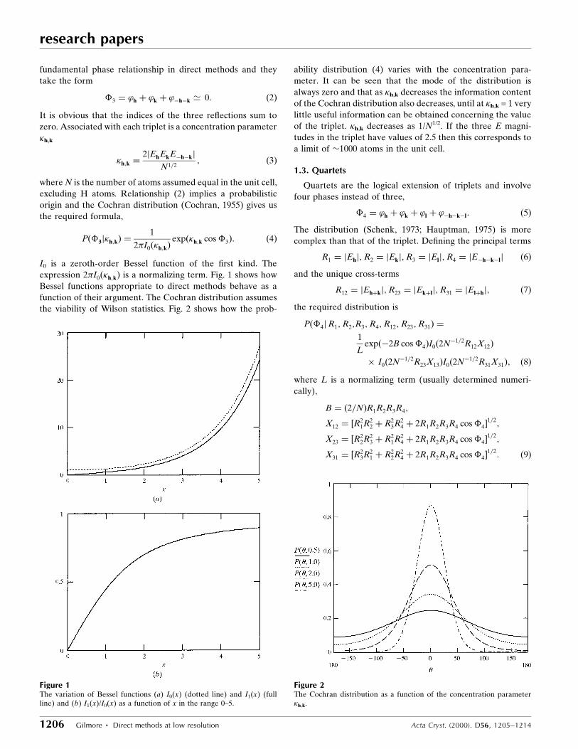
I0 is a zeroth-order Bessel function of the ®rst kind. The

expression 2�I0��h;k� is a normalizing term. Fig. 1 shows how

Bessel functions appropriate to direct methods behave as a

function of their argument. The Cochran distribution assumes

the viability of Wilson statistics. Fig. 2 shows how the prob-

ability distribution (4) varies with the concentration para-

meter. It can be seen that the mode of the distribution is

always zero and that as �h,k decreases the information content

of the Cochran distribution also decreases, until at �h,k = 1 very

little useful information can be obtained concerning the value

of the triplet. �h,k decreases as 1/N1/2. If the three E magni-

tudes in the triplet have values of 2.5 then this corresponds to

a limit of �1000 atoms in the unit cell.

1.3. Quartets

Quartets are the logical extension of triplets and involve

four phases instead of three,

�4 � 'h � 'k � 'l � 'ÿhÿkÿl: �5�The distribution (Schenk, 1973; Hauptman, 1975) is more

complex than that of the triplet. De®ning the principal terms

R1 � jEhj;R2 � jEkj;R3 � jElj;R4 � jEÿhÿkÿlj �6�and the unique cross-terms

R12 � jEh�kj;R23 � jEk�lj;R31 � jEl�hj; �7�the required distribution is

P��4jR1;R2;R3;R4;R12;R23;R31� �1

Lexp�ÿ2B cos �4�I0�2Nÿ1=2R12X12�� I0�2Nÿ1=2R23X13�I0�2Nÿ1=2R31X31�; �8�

where L is a normalizing term (usually determined numeri-

cally),

B � �2=N�R1R2R3R4;

X12 � �R21R2

2 � R23R2

4 � 2R1R2R3R4 cos �4�1=2;

X23 � �R22R2

3 � R21R2

4 � 2R1R2R3R4 cos �4�1=2;

X31 � �R23R2

1 � R22R2

4 � 2R1R2R3R4 cos �4�1=2: �9�

Figure 1The variation of Bessel functions (a) I0(x) (dotted line) and I1(x) (fullline) and (b) I1(x)/I0(x) as a function of x in the range 0±5.

Figure 2The Cochran distribution as a function of the concentration parameter�h,k.

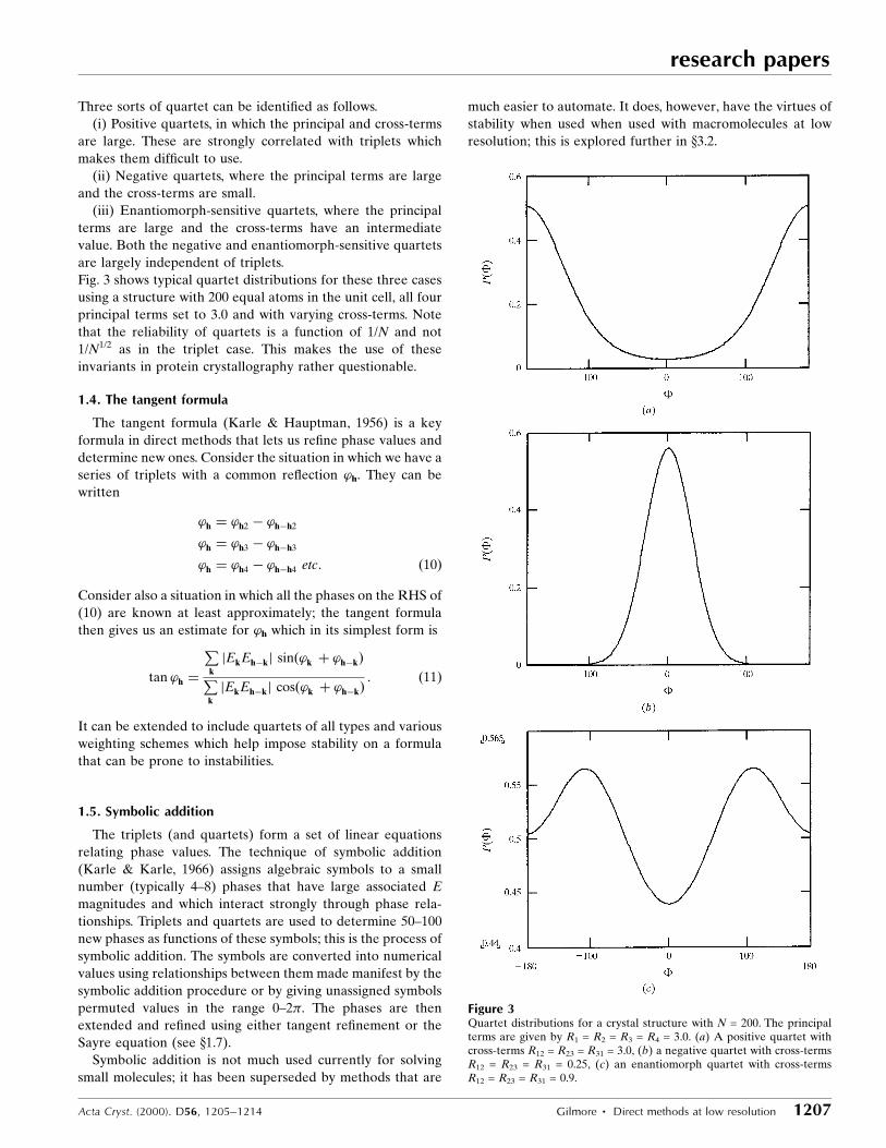
Three sorts of quartet can be identi®ed as follows.

(i) Positive quartets, in which the principal and cross-terms

are large. These are strongly correlated with triplets which

makes them dif®cult to use.

(ii) Negative quartets, where the principal terms are large

and the cross-terms are small.

(iii) Enantiomorph-sensitive quartets, where the principal

terms are large and the cross-terms have an intermediate

value. Both the negative and enantiomorph-sensitive quartets

are largely independent of triplets.

Fig. 3 shows typical quartet distributions for these three cases

using a structure with 200 equal atoms in the unit cell, all four

principal terms set to 3.0 and with varying cross-terms. Note

that the reliability of quartets is a function of 1/N and not

1/N1/2 as in the triplet case. This makes the use of these

invariants in protein crystallography rather questionable.

1.4. The tangent formula

The tangent formula (Karle & Hauptman, 1956) is a key

formula in direct methods that lets us re®ne phase values and

determine new ones. Consider the situation in which we have a

series of triplets with a common re¯ection 'h. They can be

written

'h � 'h2 ÿ 'hÿh2

'h � 'h3 ÿ 'hÿh3

'h � 'h4 ÿ 'hÿh4 etc: �10�Consider also a situation in which all the phases on the RHS of

(10) are known at least approximately; the tangent formula

then gives us an estimate for 'h which in its simplest form is

tan 'h �P

k

jEkEhÿkj sin�'k � 'hÿk�Pk

jEkEhÿkj cos�'k � 'hÿk�: �11�

It can be extended to include quartets of all types and various

weighting schemes which help impose stability on a formula

that can be prone to instabilities.

1.5. Symbolic addition

The triplets (and quartets) form a set of linear equations

relating phase values. The technique of symbolic addition

(Karle & Karle, 1966) assigns algebraic symbols to a small

number (typically 4±8) phases that have large associated E

magnitudes and which interact strongly through phase rela-

tionships. Triplets and quartets are used to determine 50±100

new phases as functions of these symbols; this is the process of

symbolic addition. The symbols are converted into numerical

values using relationships between them made manifest by the

symbolic addition procedure or by giving unassigned symbols

permuted values in the range 0±2�. The phases are then

extended and re®ned using either tangent re®nement or the

Sayre equation (see x1.7).

Symbolic addition is not much used currently for solving

small molecules; it has been superseded by methods that are

much easier to automate. It does, however, have the virtues of

stability when used when used with macromolecules at low

resolution; this is explored further in x3.2.


research papers

Figure 3Quartet distributions for a crystal structure with N = 200. The principalterms are given by R1 = R2 = R3 = R4 = 3.0. (a) A positive quartet withcross-terms R12 = R23 = R31 = 3.0, (b) a negative quartet with cross-termsR12 = R23 = R31 = 0.25, (c) an enantiomorph quartet with cross-termsR12 = R23 = R31 = 0.9.

research papers


1.6. The minimal principle

The mode of the Cochran distribution for triplets is always

zero. However, the mean can be computed as

hcos �3i �R�0

cos �3P��3j�h;k� �I1��h;k�I0��h;k�

: �12�

This expression gives rise to the minimal function (DeTitta et

al., 1994)

R��3� �Ph;k

�h;k cos Th;k ÿI1��h;k�I0��h;k�

� �2�Ph;k

�h;k; �13�

where cosTh,k is the value of the triplet computed from known

phases. The function R(�3) serves two purposes: (i) as a

formula to re®ne and estimate new phases by minimizing the

difference between the estimated value and the mean of the

cosine of the triplet and (ii) as the minimal principle which

uses (13) to de®ne the best phase set, i.e. as a ®gure of merit.

1.7. The Sayre equation

The Sayre equation (Sayre, 1952) is algebraic rather than

probabilistic in origin and is derived from the expression for

the electron density and its square,

Fh � ��=V�Pk

FkFhÿk: �14�

In terms of E magnitudes this takes the form of the Sayre±

Hughes (Hughes, 1953) equation,

Eh � N1=2hEkEhÿki: �15�The Sayre equation can be used in the same way as the tangent

formula, but has a more general validity and is not constrained

to use only large structure-factor magnitudes.

1.8. Figures of merit

In general, direct methods are multi-solutional: they give

rise to multiple phase sets and we need to select those which

are most likely to give useful structural information. Figures of

merit serve this purpose and are used to rank phase sets. There

are numerous such indicators, including the following. (i) The

minimal function (13). An optimal phase set will have a

minimum value of R(�3). (ii) The negative quartet ®gure of

merit (DeTitta et al., 1975),

NQEST �

Pnegative

B cos�'h � 'k � 'l � 'ÿhÿkÿl�Pnegative

B; �16�

where the summation spans all those quartets assumed

negative using (8). An optimal phase set should have a

minimum value of NQEST.

Usually, several ®gures of merit are calculated for a given

phase set and these are combined to given an overall ®gure

called a CFOM.

1.9. Correlation coefficients

Let Eo be the observed E magnitude and Ec the calculated

value from, for example, a variant of the tangent formula; let w

be the associated weight. For a set of such magnitudes we can

then compute the correlation coef®cient CC, which takes

many forms. A useful expression from Read (1986) is

CC � PwE2

oE2c

PwÿPwE2

o

PwE2

c

ÿ �=ÿ��P

wE4o

Pwÿ ÿPwE2

o

�2�� PwE4

c

Pwÿ ÿPwE2

c

�2�1=2�: �17�

Correlation coef®cients lie between ÿ1 � CC � 1.0. They can

be used as ®gures of merit.

1.10. E maps

So far our discussions have involved reciprocal-space

quantities; the transform into real space is carried out using E

magnitudes via E maps,

��x� ' 1

V

Ph

jEhj exp�i'h� exp�ÿ2�ih � x�: �18�

The use of E magnitudes and the limits we shall impose on the

re¯ections entering the summation in (16) mean that the

electron density is only approximate (at the very least, there

are serious series-termination errors), but hopefully is suf®-

cient to reveal structural features so that model building can

begin.

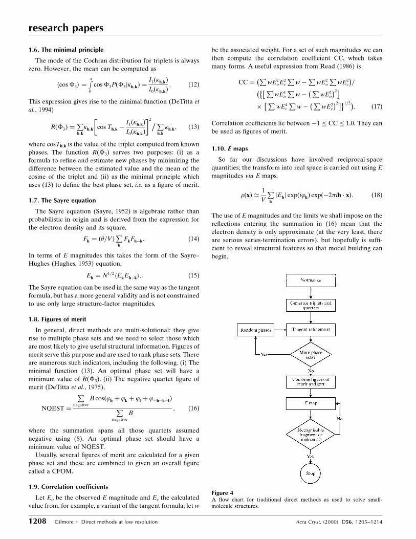
Figure 4A ¯ow chart for traditional direct methods as used to solve small-molecule structures.

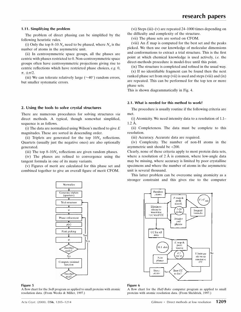
1.11. Simplifying the problem

The problem of direct phasing can be simpli®ed by the

following heuristic rules.

(i) Only the top 8±10 Na need to be phased, where Na is the

nunber of atoms in the asymmetric unit.

(ii) In centrosymmetric space groups, all the phases are

centric with phases restricted to 0. Non-centrosymmetric space

groups often have centrosymmetric projections giving rise to

centric re¯ections which have restricted phase choices, e.g. 0,

�, ��/2.

(iii) We can tolerate relatively large (�40�) random errors,

but smaller systematic errors.

2. Using the tools to solve crystal structures

There are numerous procedures for solving structures via

direct methods. A typical, though somewhat simpli®ed,

sequence is as follows.

(i) The data are normalized using Wilson's method to give E

magnitudes. These are sorted in descending order.

(ii) Triplets are generated for the top 10Na re¯ections.

Quartets (usually just the negative ones) are also optionally

generated.

(iii) The top 8±10Na re¯ections are given random phases.

(iv) The phases are re®ned to convergence using the

tangent formula in one of its many variants.

(v) Figures of merit are calculated for this phase set and

combined together to give an overall ®gure of merit CFOM.

(vi) Steps (iii)±(v) are repeated 24±1000 times depending on

the dif®culty and complexity of the structure.

(vii) The phase sets are sorted on CFOM.

(viii) An E map is computed for the best set and the peaks

picked. We then use our knowledge of molecular dimensions

and conformations to extract a trial structure. This is the ®rst

point at which chemical knowledge is used actively, i.e. the

direct-methods procedure is model-free until this point.

(ix) The structure is completed and re®ned in the usual way.

(x) If no identi®able fragment can be found then the next

ranked phase set from step (vii) is used and steps (viii) and (ix)

are repeated. This can be performed for the top ten or more

phase sets.

This is shown diagrammatically in Fig. 4.

2.1. What is needed for this method to work?

The procedure is usually routine if the following criteria are

met.

(i) Atomicity. We need intensity data to a resolution of 1.1±

1.2 AÊ .

(ii) Completeness. The data must be complete to this

resolution.

(iii) Accuracy. Accurate data are required.

(iv) Complexity. The number of non-H atoms in the

asymmetric unit should be <200.

Clearly, none of these criteria apply to most protein data sets,

where a resolution of 2 AÊ is common, where low-angle data

may be missing, where accuracy is limited by poor crystalline

specimens and where the number of atoms in the asymmetric

unit is several thousand.

This latter problem can be overcome using atomicity as a

stronger constraint and this gives rise to the computer


research papers

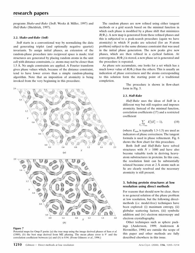
Figure 6A ¯ow chart for the Half-Bake computer program as applied to smallproteins with atomic resolution data. (From Sheldrick, 1997.)

Figure 5A ¯ow chart for the SnB program as applied to small proteins with atomicresolution data. (From Weeks & Miller, 1997.)

research papers


programs Shake-and-Bake (SnB; Weeks & Miller, 1997) and

Half-Bake (Sheldrick, 1997).

2.2. Shake-and-Bake (SnB)

SnB starts in a conventional way by normalizing the data

and generating triplet (and optionally negative quartet)

invariants. To assign initial phases, an extension of the

random-phase procedure into reciprocal space is made; trial

structures are generated by placing random atoms in the unit

cell with distance constraints, i.e. atoms may not be closer than

1.5 AÊ . No angle constraints are applied. A Fourier transform

gives phase values which, because of the distance constraint,

tend to have lower errors than a simple random-phasing

algorithm. Note that an imposition of atomicity is being

invoked from the very beginning in this procedure.

The random phases are now re®ned using either tangent

methods or a grid search based on the minimal function in

which each phase is modi®ed by a phase shift that minimizes

R(�3). A new map is generated from these re®ned phases and

this is subjected to a peak-search procedure (again we have

atomicity) in which N peaks are selected (for an N-atom

problem) subject to the same distance constraint that was used

in the initial phase generation. The new peaks give new

phases, which are then re®ned in a cyclical fashion. At

convergence, R(�3) is stored, a new phase set is generated and

the procedure is repeated.

As phase sets accumulate, one looks for a set which has a

much lower value of R(�3) than the others. This is usually an

indication of phase correctness and the atoms corresponding

to this solution form the starting point of a traditional

completion.

The procedure is shown in ¯ow-chart

form in Fig. 5.

2.3. Half-Bake

Half-Bake uses the ideas of SnB in a

different way but still requires and imposes

atomicity. Instead of the minimal function,

correlation coef®cients (17) and a restricted

coef®cient PEo>Emin

E2c�E2

o ÿ 1�; �19�

(where Emin is typically 1.3±1.5) are used as

indicators of phase correctness. The tangent

formula is used in phase re®nement. Fig. 6

shows the ¯ow chart for this procedure.

Both SnB and Half-Bake have solved

structures with N > 1000 and have also

become valuable tools in deriving heavy-

atom substructures in proteins. In this case,

the resolution limit can be substantially

relaxed because even at 2 AÊ atoms such as

Se are clearly resolved and the necessary

atomicity is still present.

3. Solving protein structures at lowresolution using direct methods

For reasons that should now be clear, there

is no general solution of the phase problem

at low resolution, but the following direct-

methods (i.e. model-free) techniques have

been explored: (i) maximum entropy, (ii)

globular scattering factors, (iii) symbolic

addition and (iv) electron microscopy and

electron crystallography.

Other techniques such as sphere pack-

ings (Andersson, 1999; Andersson &

HovmoÈ ller, 1996) are outside the scope of

this paper and other methods are fully

described elsewhere in this issue.

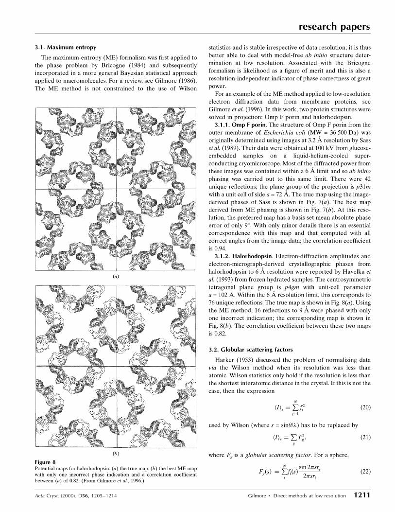
Figure 7Potential maps for Omp F porin: (a) the true map using the image derived phases of Sass et al.(1989), (b) the best map derived from ME phasing. The mean phase error is 9� and thecorrelation coef®cient between (a) and (b) is 0.94. (From Gilmore et al., 1996.)

3.1. Maximum entropy

The maximum-entropy (ME) formalism was ®rst applied to

the phase problem by Bricogne (1984) and subsequently

incorporated in a more general Bayesian statistical approach

applied to macromolecules. For a review, see Gilmore (1986).

The ME method is not constrained to the use of Wilson

statistics and is stable irrespective of data resolution; it is thus

better able to deal with model-free ab initio structure deter-

mination at low resolution. Associated with the Bricogne

formalism is likelihood as a ®gure of merit and this is also a

resolution-independent indicator of phase correctness of great

power.

For an example of the ME method applied to low-resolution

electron diffraction data from membrane proteins, see

Gilmore et al. (1996). In this work, two protein structures were

solved in projection: Omp F porin and halorhodopsin.

3.1.1. Omp F porin. The structure of Omp F porin from the

outer membrane of Escherichia coli (MW = 36 500 Da) was

originally determined using images at 3.2 AÊ resolution by Sass

et al. (1989). Their data were obtained at 100 kV from glucose-

embedded samples on a liquid-helium-cooled super-

conducting cryomicroscope. Most of the diffracted power from

these images was contained within a 6 AÊ limit and so ab initio

phasing was carried out to this same limit. There were 42

unique re¯ections; the plane group of the projection is p31m

with a unit cell of side a = 72 AÊ . The true map using the image-

derived phases of Sass is shown in Fig. 7(a). The best map

derived from ME phasing is shown in Fig. 7(b). At this reso-

lution, the preferred map has a basis set mean absolute phase

error of only 9�. With only minor details there is an essential

correspondence with this map and that computed with all

correct angles from the image data; the correlation coef®cient

is 0.94.

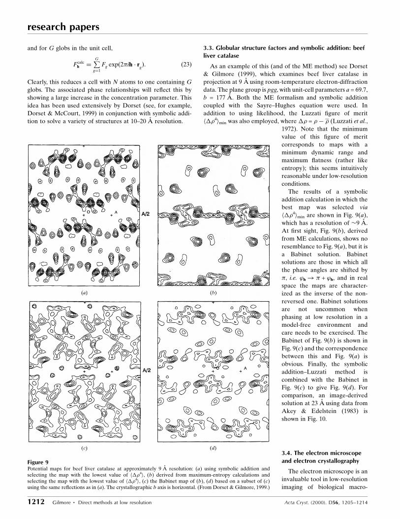
3.1.2. Halorhodopsin. Electron-diffraction amplitudes and

electron-micrograph-derived crystallographic phases from

halorhodopsin to 6 AÊ resolution were reported by Havelka et

al. (1993) from frozen hydrated samples. The centrosymmetric

tetragonal plane group is p4gm with unit-cell parameter

a = 102 AÊ . Within the 6 AÊ resolution limit, this corresponds to

76 unique re¯ections. The true map is shown in Fig. 8(a). Using

the ME method, 16 re¯ections to 9 AÊ were phased with only

one incorrect indication; the corresponding map is shown in

Fig. 8(b). The correlation coef®cient between these two maps

is 0.82.

3.2. Globular scattering factors

Harker (1953) discussed the problem of normalizing data

via the Wilson method when its resolution was less than

atomic. Wilson statistics only hold if the resolution is less than

the shortest interatomic distance in the crystal. If this is not the

case, then the expression

hIis �PNj�1

f 2j �20�

used by Wilson (where s = sin�/�) has to be replaced by

hIis �P

g

F2g ; �21�

where Fg is a globular scattering factor. For a sphere,

Fg�s� �PN

i

fi�s�sin 2�sri

2�sri

�22�


research papers

Figure 8Potential maps for halorhodopsin: (a) the true map, (b) the best ME mapwith only one incorrect phase indication and a correlation coef®cientbetween (a) of 0.82. (From Gilmore et al., 1996.)

research papers


and for G globs in the unit cell,

Fcalch � PG

g�1

Fg exp�2�ih � rg�: �23�

Clearly, this reduces a cell with N atoms to one containing G

globs. The associated phase relationships will re¯ect this by

showing a large increase in the concentration parameter. This

idea has been used extensively by Dorset (see, for example,

Dorset & McCourt, 1999) in conjunction with symbolic addi-

tion to solve a variety of structures at 10±20 AÊ resolution.

3.3. Globular structure factors and symbolic addition: beefliver catalase

As an example of this (and of the ME method) see Dorset

& Gilmore (1999), which examines beef liver catalase in

projection at 9 AÊ using room-temperature electron-diffraction

data. The plane group is pgg, with unit-cell parameters a = 69.7,

b = 177 AÊ . Both the ME formalism and symbolic addition

coupled with the Sayre±Hughes equation were used. In

addition to using likelihood, the Luzzati ®gure of merit

h��4imin was also employed, where �� = � ÿ � (Luzzati et al.,

1972). Note that the minimum

value of this ®gure of merit

corresponds to maps with a

minimum dynamic range and

maximum ¯atness (rather like

entropy); this seems intuitively

reasonable under low-resolution

conditions.

The results of a symbolic

addition calculation in which the

best map was selected via

h��4imin are shown in Fig. 9(a),

which has a resolution of �9 AÊ .

At ®rst sight, Fig. 9(b), derived

from ME calculations, shows no

resemblance to Fig. 9(a), but it is

a Babinet solution. Babinet

solutions are those in which all

the phase angles are shifted by

�, i.e. 'h! � + 'h, and in real

space the maps are character-

ized as the inverse of the non-

reversed one. Babinet solutions

are not uncommon when

phasing at low resolution in a

model-free environment and

care needs to be exercised. The

Babinet of Fig. 9(b) is shown in

Fig. 9(c) and the correspondence

between this and Fig. 9(a) is

obvious. Finally, the symbolic

addition±Luzzati method is

combined with the Babinet in

Fig. 9(c) to give Fig. 9(d). For

comparison, an image-derived

solution at 23 AÊ using data from

Akey & Edelstein (1983) is

shown in Fig. 10.

3.4. The electron microscopeand electron crystallography

The electron microscope is an

invaluable tool in low-resolution

imaging of biological macro-

Figure 9Potential maps for beef liver catalase at approximately 9 AÊ resolution: (a) using symbolic addition andselecting the map with the lowest value of h��4i, (b) derived from maximum-entropy calculations andselecting the map with the lowest value of h��4i, (c) the Babinet map of (b), (d) based on a subset of (c)using the same re¯ections as in (a). The crystallographic b axis is horizontal. (From Dorset & Gilmore, 1999.)

molecules. It is the source of two sorts of data for crystal-

lographic purposes.

(i) Phased re¯ections, where the phase information comes

from the Fourier transform of electron-microscope images

after suitable ®ltering. Usually the phases so derived corre-

spond to intensities that have a signi®cantly lower resolution

than the diffraction data and there are some signi®cant

sources of error in image data arising from radiation damage,

curvilinear paracrystalline distortion and transfer-function

uncertainties, but they are invaluable.

(ii) The electron diffraction data, which are less problematic

and have a higher resolution than those in (i). Clearly, to

achieve optimum resolution we need to extend the image-

derived phases to phase the diffraction intensities and this is a

problem that direct methods can address.

Two sorts of situation arise in phase extension as follows.

(i) The image phase set is suf®ciently large and well

distributed in reciprocal space to permit an unambiguous

phase-extension procedure without recourse to multi-solution

methods, i.e. those that involve phase permutation.

(ii) When the basis set is small or in some way inadequate

we have a branching problem. This problem arises when

phases are selected without exploring the relevant phase space

in suf®cient detail, so that what appears to be an unambiguous

phase choice is no such thing. The methods outlined in x3 can

be employed here; for a survey of electron crystallography and

these problems in an ME context, see Gilmore (1996).

3.5. The use of very low resolution reflections

Traditional wisdom dictates that very low angle re¯ections

in protein crystallography are of minimal value and their use

can prevent a successful structure solution. This is effectively

refuted by Andersson (1999) and by the results presented

above where the very low order re¯ections played a key role.

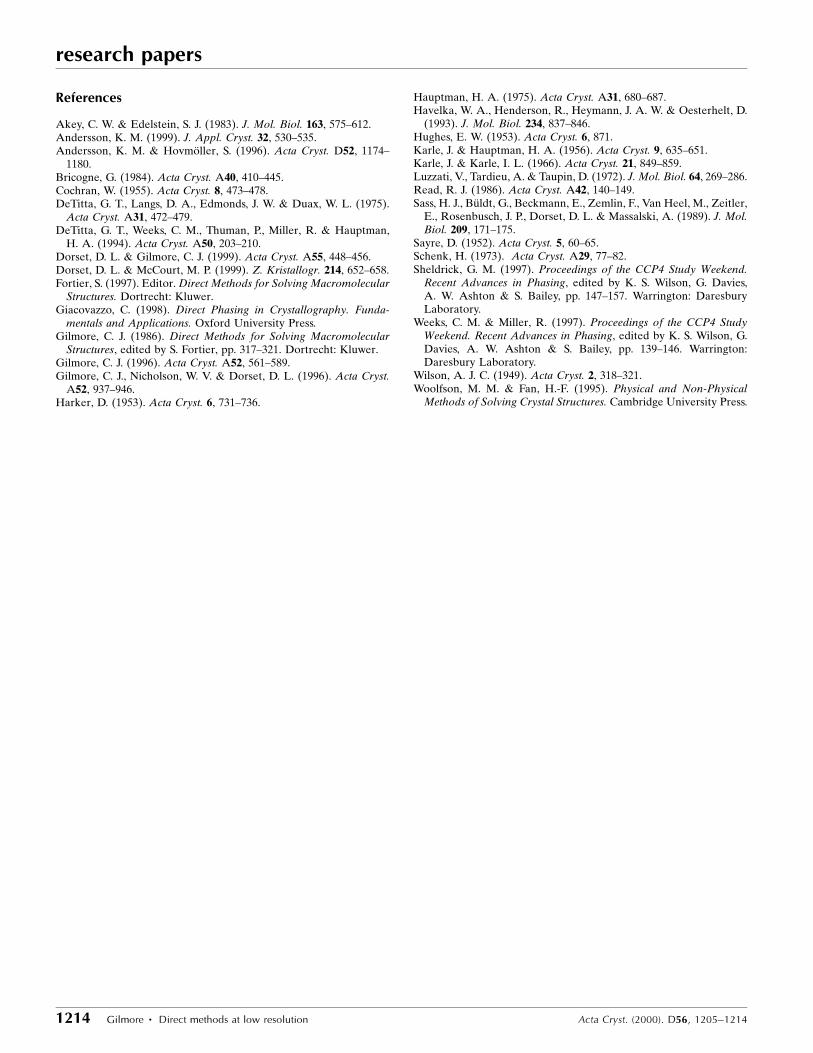
To summarize his arguments: the solvent contribution to a

given re¯ection depends on the difference between the elec-

tron density of the solvent and that of the protein. At very low

resolution, the Babinet principle means that the phases of the

solvent are shifted by � relative to the protein (see Fig. 11).

The correlation coef®cient is close to 100% to 15 AÊ resolution,

but becomes effectively zero at less than 3 AÊ . This means that

no bulk-solvent correction is needed when using only low-

angle re¯ections. When mixing data at low and high resolution

then the magnitude of the solvent vector depends on the

solvent±protein contrast and we can write the total structure

factor |Fh|total as

jFhjtotal � jFhjp ÿ ksjFhjp exp�ÿBs sin2 �=�2�; �24�

where ks measures the density ratio of solvent and protein and

Bs is the solvent temperature factor. Thus, properly handled,

there is no reason to exclude low-order data from ab intio

structure determination.

I wish to acknowledge invaluable and stimulating discus-

sions with Klas Andersson and Doug Dorset and support from

Eastman-Kodak (Rochester), EPSRC and BBSRC.


research papers

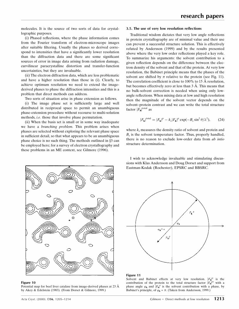
Figure 10Potential map for beef liver catalase from image-derived phases at 23 AÊ

by Akey & Edelstein (1983). (From Dorset & Gilmore, 1999.)

Figure 11Solvent and Babinet effects at very low resolution. |Fh|p is thecontribution of the protein to the total structure factor |Fh|ps with aphase angle 'h and |Fh|s is the solvent contribution with a phase, byBabinet's principle, of 'h + �. (Taken from Andersson, 1999.)

research papers


References

Akey, C. W. & Edelstein, S. J. (1983). J. Mol. Biol. 163, 575±612.Andersson, K. M. (1999). J. Appl. Cryst. 32, 530±535.Andersson, K. M. & HovmoÈ ller, S. (1996). Acta Cryst. D52, 1174±

1180.Bricogne, G. (1984). Acta Cryst. A40, 410±445.Cochran, W. (1955). Acta Cryst. 8, 473±478.DeTitta, G. T., Langs, D. A., Edmonds, J. W. & Duax, W. L. (1975).

Acta Cryst. A31, 472±479.DeTitta, G. T., Weeks, C. M., Thuman, P., Miller, R. & Hauptman,

H. A. (1994). Acta Cryst. A50, 203±210.Dorset, D. L. & Gilmore, C. J. (1999). Acta Cryst. A55, 448±456.Dorset, D. L. & McCourt, M. P. (1999). Z. Kristallogr. 214, 652±658.Fortier, S. (1997). Editor. Direct Methods for Solving Macromolecular

Structures. Dortrecht: Kluwer.Giacovazzo, C. (1998). Direct Phasing in Crystallography. Funda-

mentals and Applications. Oxford University Press.Gilmore, C. J. (1986). Direct Methods for Solving Macromolecular

Structures, edited by S. Fortier, pp. 317±321. Dortrecht: Kluwer.Gilmore, C. J. (1996). Acta Cryst. A52, 561±589.Gilmore, C. J., Nicholson, W. V. & Dorset, D. L. (1996). Acta Cryst.

A52, 937±946.Harker, D. (1953). Acta Cryst. 6, 731±736.

Hauptman, H. A. (1975). Acta Cryst. A31, 680±687.Havelka, W. A., Henderson, R., Heymann, J. A. W. & Oesterhelt, D.

(1993). J. Mol. Biol. 234, 837±846.Hughes, E. W. (1953). Acta Cryst. 6, 871.Karle, J. & Hauptman, H. A. (1956). Acta Cryst. 9, 635±651.Karle, J. & Karle, I. L. (1966). Acta Cryst. 21, 849±859.Luzzati, V., Tardieu, A. & Taupin, D. (1972). J. Mol. Biol. 64, 269±286.Read, R. J. (1986). Acta Cryst. A42, 140±149.Sass, H. J., BuÈ ldt, G., Beckmann, E., Zemlin, F., Van Heel, M., Zeitler,

E., Rosenbusch, J. P., Dorset, D. L. & Massalski, A. (1989). J. Mol.Biol. 209, 171±175.

Sayre, D. (1952). Acta Cryst. 5, 60±65.Schenk, H. (1973). Acta Cryst. A29, 77±82.Sheldrick, G. M. (1997). Proceedings of the CCP4 Study Weekend.

Recent Advances in Phasing, edited by K. S. Wilson, G. Davies,A. W. Ashton & S. Bailey, pp. 147±157. Warrington: DaresburyLaboratory.

Weeks, C. M. & Miller, R. (1997). Proceedings of the CCP4 StudyWeekend. Recent Advances in Phasing, edited by K. S. Wilson, G.Davies, A. W. Ashton & S. Bailey, pp. 139±146. Warrington:Daresbury Laboratory.

Wilson, A. J. C. (1949). Acta Cryst. 2, 318±321.Woolfson, M. M. & Fan, H.-F. (1995). Physical and Non-Physical

Methods of Solving Crystal Structures. Cambridge University Press.

Documents

Direct methods and protein crystallography at low resolution