Direct Nuclear Reactions

N. Keeley

National Centre for Nuclear Research

The aim of these lectures:

1) What is a direct reaction?

2) Why should we study them?

3) How do we interpret them?

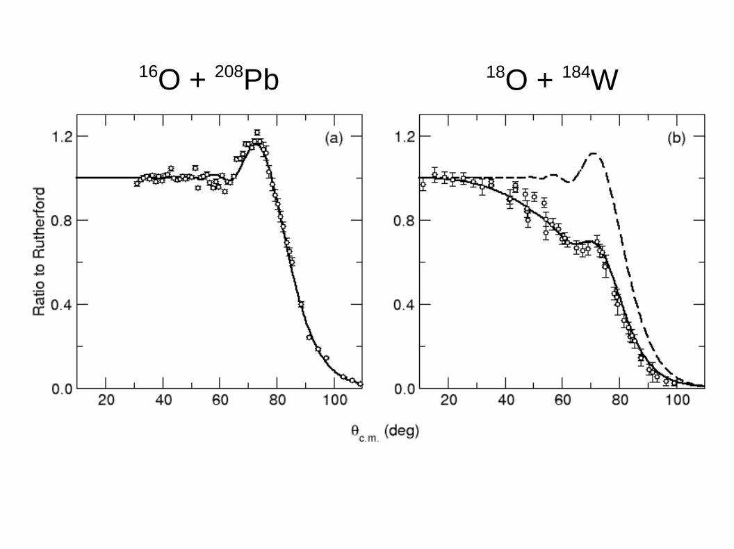
16O + 208Pb 18O + 184W

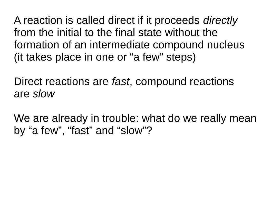
A reaction is called direct if it proceeds directlyfrom the initial to the final state without the formation of an intermediate compound nucleus(it takes place in one or “a few” steps)

Direct reactions are fast, compound reactions are slow

We are already in trouble: what do we really meanby “a few”, “fast” and “slow”?

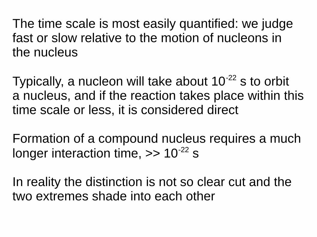
The time scale is most easily quantified: we judgefast or slow relative to the motion of nucleons inthe nucleus

Typically, a nucleon will take about 10-22 s to orbita nucleus, and if the reaction takes place within thistime scale or less, it is considered direct

Formation of a compound nucleus requires a muchlonger interaction time, >> 10-22 s

In reality the distinction is not so clear cut and thetwo extremes shade into each other

As for the number of steps involved, the distinctionis even less clear-cut.

A single-step reaction is clearly direct, but …

As the projectile interacts successively it penetratesthe target more deeply until eventually a compoundnucleus is formed. However, the reaction mayterminate after only a few interactions. Is this stilldirect? The distinction is often largely a question ofpersonal taste.

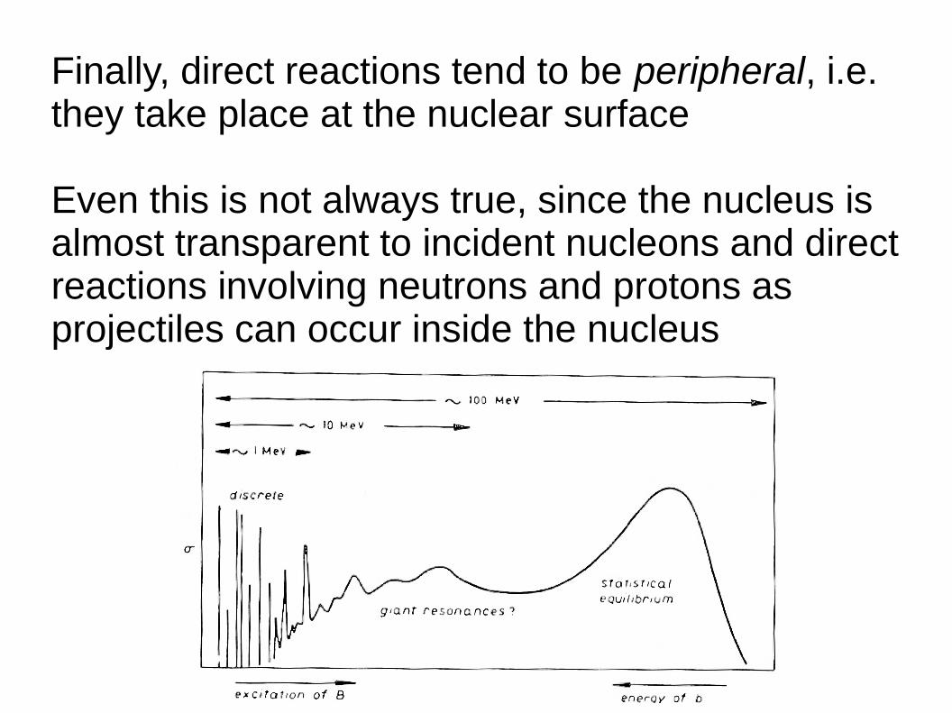
Finally, direct reactions tend to be peripheral, i.e.they take place at the nuclear surface

Even this is not always true, since the nucleus isalmost transparent to incident nucleons and directreactions involving neutrons and protons asprojectiles can occur inside the nucleus

What are the different types of (direct) reaction?

Some nomenclature:

We write a reaction thus:

A + a → B + b + Q

A is the target, a the projectile, B the residual, b the ejectile and Q is the “Q value”.

This is written more concisely as:

A(a,b)B

Each possible combination of particles is referredto as a partition. Further, within a partition we mayspecify the state of excitation of each nucleus.Such a pair of nuclei each in a specific state isknown as a channel. Each partition can in principle consist of many channels.

Thus the combination A + a is known as theentrance channel (both nuclei are in their groundstates). The various possible sets of products Band b in their specific excitation states constitutethe exit channels.

The Q value is simply the energy released duringthe reaction. It is most simply defined as:

Q = Ef − E

i

If the Q value is negative the reaction is termedendothermic, i.e. the final total kinetic energy is less than the initial.

If the Q value is positive we have an exothermicreaction, and binding energy (or rest mass) isreleased during the reaction

For negative Q, there is a threshold energy sinceE

f must be > 0, E

i = E

th = −Q

Back to the various classes of (direct) reaction …

1) Elastic scattering. The simplest “reaction”. Theinternal states of a and A are unchanged and Q = 0.Written as: A(a,a)A

2) Inelastic scattering. Usually, this term is appliedto a reaction where A is left in an excited state, i.e.B = A* and therefore Q = − E

x. a is then emitted

with reduced energy and the reaction is written as:A(a,a′)A*. For complex projectiles a may be excited instead of the target or both a and A may be left in excited states (mutual excitation).

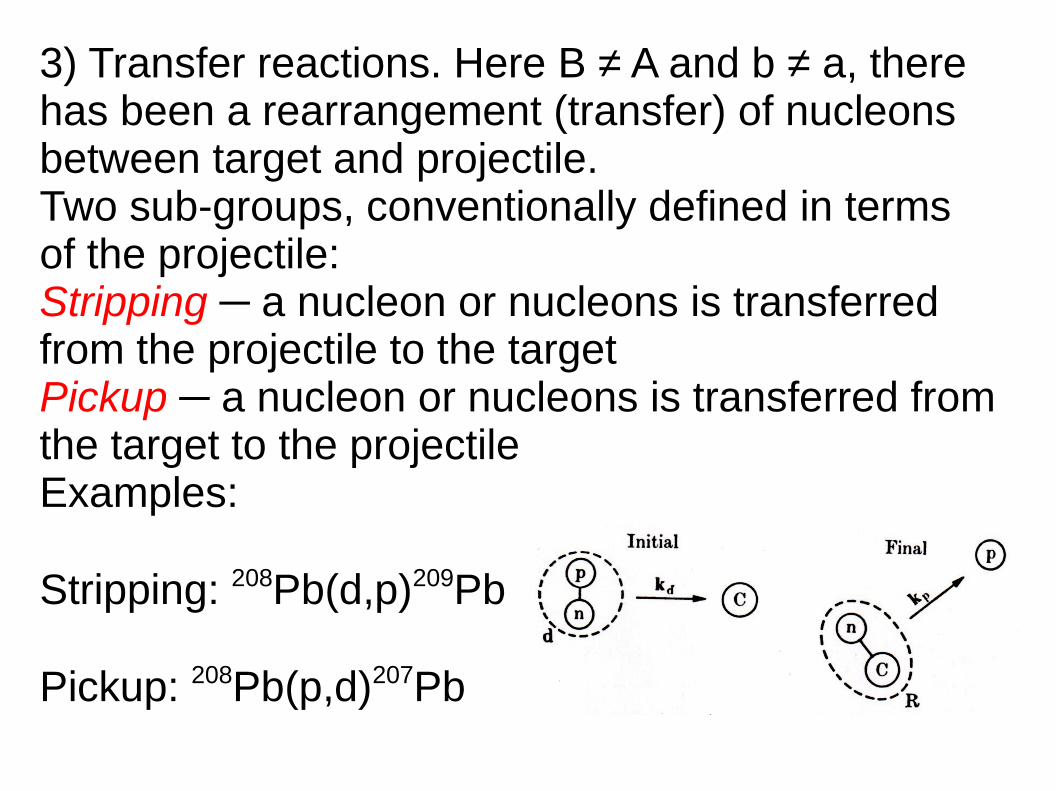
3) Transfer reactions. Here B ≠ A and b ≠ a, therehas been a rearrangement (transfer) of nucleonsbetween target and projectile. Two sub-groups, conventionally defined in terms of the projectile: Stripping ─ a nucleon or nucleons is transferred from the projectile to the targetPickup ─ a nucleon or nucleons is transferred fromthe target to the projectileExamples:

Stripping: 208Pb(d,p)209Pb

Pickup: 208Pb(p,d)207Pb

4) Breakup. This is no longer a simple two-bodyprocess but (usually) a three-body one:

A(a,a*→b + c)A

i.e. a is excited to a “state” (either a resonance orthe continuum) above the emission threshold forparticle c (a is considered to consist of particle cbound to core b)

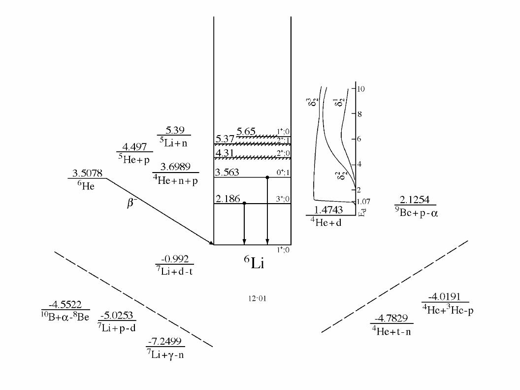
Example: 6Li* → α + d

Four-body (or more) breakup modes can also occur,e.g. 6He → α + n + n

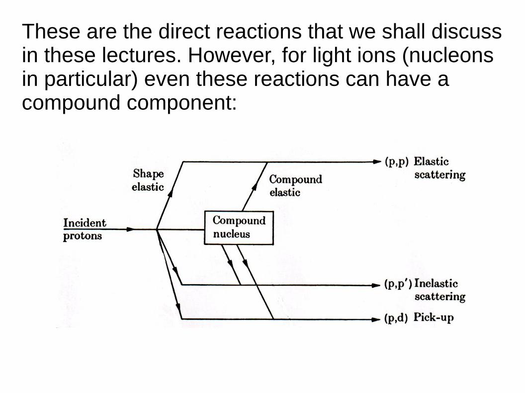
These are the direct reactions that we shall discussin these lectures. However, for light ions (nucleonsin particular) even these reactions can have acompound component:

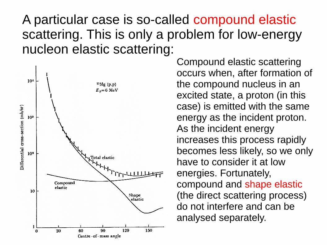
A particular case is so-called compound elasticscattering. This is only a problem for low-energynucleon elastic scattering:

Compound elastic scattering occurs when, after formation of the compound nucleus in an excited state, a proton (in this case) is emitted with the same energy as the incident proton. As the incident energy increases this process rapidly becomes less likely, so we only have to consider it at low energies. Fortunately, compound and shape elastic (the direct scattering process) do not interfere and can be analysed separately.

Finally, if the projectile has exactly the right energyresonant behaviour can occur (usually only inelastic or inelastic scattering). This is not confinedto nucleons or light ions, it can also occur for thelighter heavy ions (a heavy ion is by convention anything heavier than an α particle). However, it usually only occurs at low incident energies andwe shall not consider it further here.

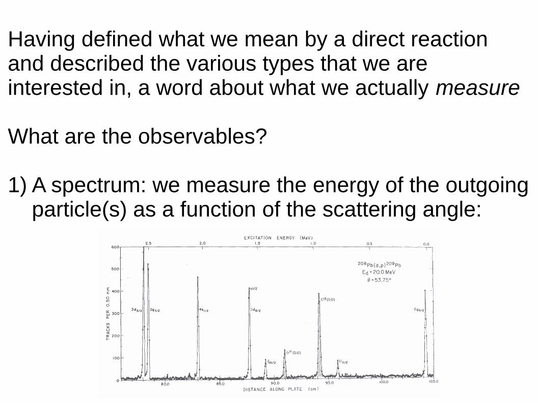
Having defined what we mean by a direct reactionand described the various types that we areinterested in, a word about what we actually measure

What are the observables?

1) A spectrum: we measure the energy of the outgoing particle(s) as a function of the scattering angle:

2) We can count the number of outgoing particles (of a particular type) either in total or as a function of angle. This is usually reduced to a “standardised” number, the cross section

Remember that any other “experimental” quantities are in fact derived from these observables using models

How is cross section defined? Although it has unitsof area (usually measured in barns ― symbol b, 1b = 10-28 m2 ― or sub-multiples thereof in nuclear physics) it is really a measure of the probability that a particular reaction will occur.

Returning to our typical reaction A(a,b)B. If we haveI0 particles of type a per unit area incident on a

target containing N particles of type A then the number of particles b that we detect is obviouslyproportional to I

0 and N, the constant of

proportionality being the cross section, σ:

σ = number of particles b detected I

0 x N

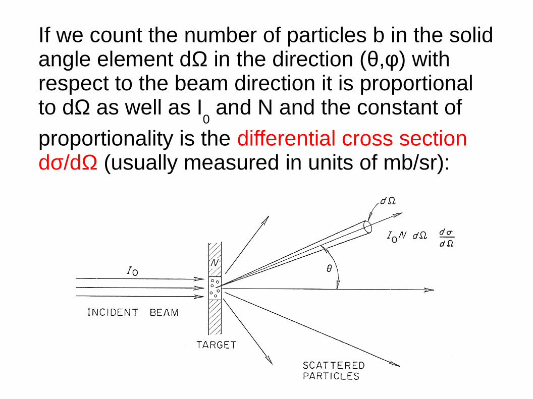
If we count the number of particles b in the solidangle element dΩ in the direction (θ,φ) with respect to the beam direction it is proportionalto dΩ as well as I

0 and N and the constant of

proportionality is the differential cross sectiondσ/dΩ (usually measured in units of mb/sr):

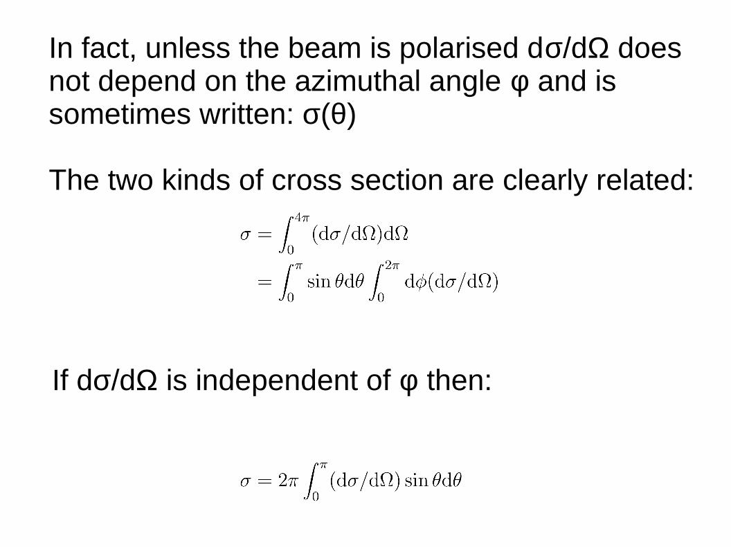
In fact, unless the beam is polarised dσ/dΩ doesnot depend on the azimuthal angle φ and is sometimes written: σ(θ)

The two kinds of cross section are clearly related:

If dσ/dΩ is independent of φ then:

In direct reaction work we usually measure theangular distribution of the differential cross section,since this contains most of the information (as weshall see later on).

However, sometimes the cross section σ is measured.If we measure σ for each type of particle emitted in anon-elastic process this is called the reaction crosssection. If we then add σ

el to this number we obtain

the total cross section, a measure of the probabilitythat something will occur during the collision

The reaction cross section, σR, is the most useful of

these quantities and we shall meet it again later.

Finally, a word about books:

Introduction to Nuclear Reactions, G. R. Satchlertwo editions, 1980 and 1991 (paperback). Still thebest introduction to the subject but long out of printand difficult to find.

Direct Nuclear Reactions, G. R. Satchler, OUP 1983.Long out of print and very difficult to find. Still a verygood monograph on the subject.

Nuclear Reactions and Nuclear Structure, P. E. Hodgson, OUP 1971. Also long out of print anddifficult to find. A good monograph on light-ion induced reactions and their analysis.

Nuclear Reactions for Astrophysics: Principles, Calculation and Applications of Low-Energy Reactions, I. J. Thompson and F. M. Nunes, CUP2009. Perhaps the best of the in-print books on thesubject. Linked to practical use of the direct reactioncode FRESCO.

Lecture 2: Kinematics

“Kinematics” covers a multitude of sins. In this lecturewe shall define some more quantities that will beuseful later and look at the consequences of someconservation laws.

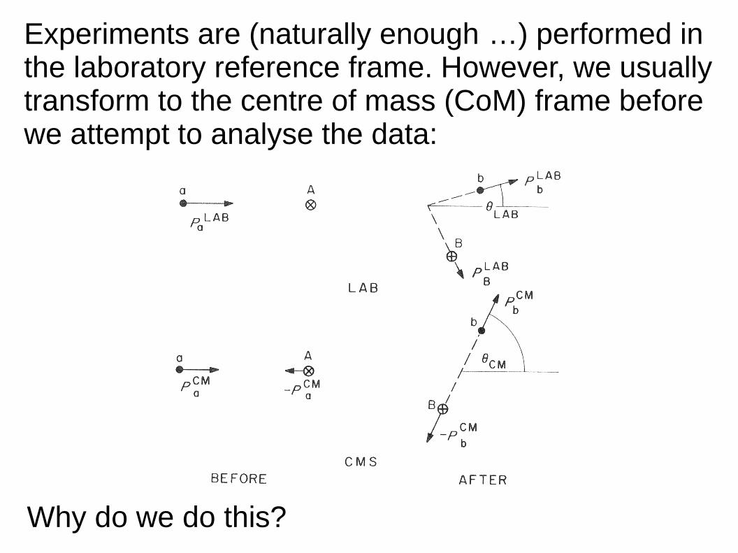
Experiments are (naturally enough …) performed inthe laboratory reference frame. However, we usuallytransform to the centre of mass (CoM) frame beforewe attempt to analyse the data:

Why do we do this?

It makes life easier! One conserved quantity in anuclear collision is the total momentum. We thuschose a reference system where the total momentum is 0 – the centre of mass system.

Here, the centre of mass of the projectile-target system is at rest and the projectile and targetapproach each other with equal and oppositemomenta: P′

a = −P′

A . Since total momentum is

conserved, P′b = −P′

B if there are only two products.

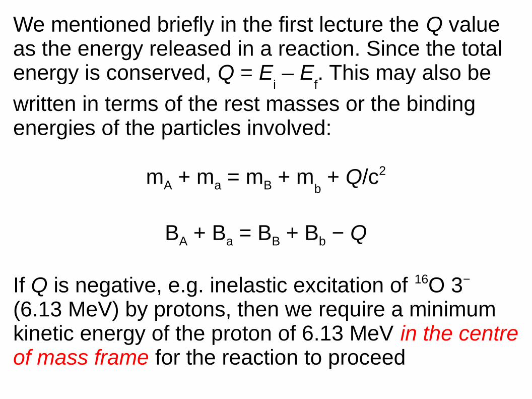
We mentioned briefly in the first lecture the Q valueas the energy released in a reaction. Since the totalenergy is conserved, Q = E

i – E

f. This may also be

written in terms of the rest masses or the binding energies of the particles involved:

mA + ma = mB + mb + Q/c2

BA + Ba = BB + Bb − Q

If Q is negative, e.g. inelastic excitation of 16O 3− (6.13 MeV) by protons, then we require a minimum kinetic energy of the proton of 6.13 MeV in the centreof mass frame for the reaction to proceed

The kinetic energy of the motion of the centre of mass of the system is conserved and is therefore not available for producing nuclear excitations: advantageof CoM system is that it is zero (CoM at rest, bydefinition) so we do not need to worry about it!

Other conserved quantities are total charge, numberof neutrons and protons (in the reactions we willconsider; it is not always so), the parity and the totalangular momentum. Any change in the total (vectorsum) of the intrinsic spins of the nuclei must be compensated for by a change in the orbital angularmomentum of their relative motion. Likewise for theproduct of their intrinsic parities.

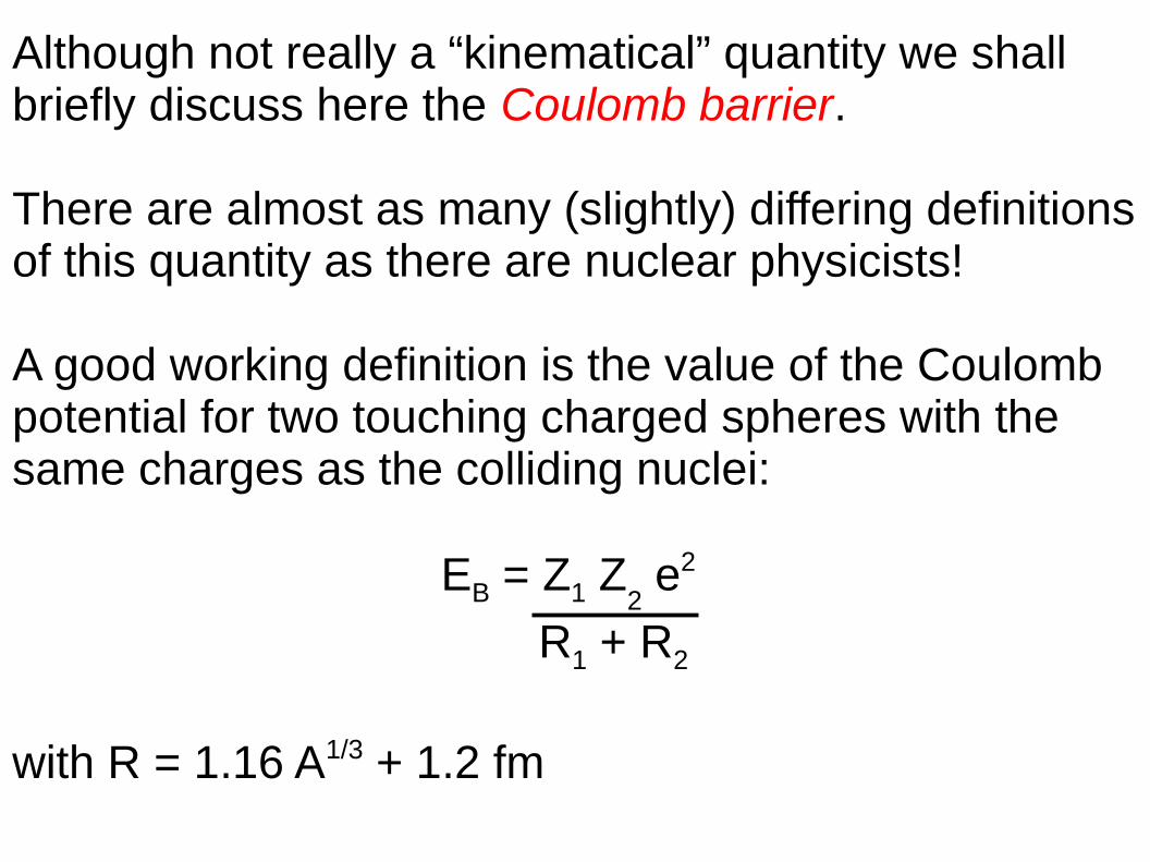
Although not really a “kinematical” quantity we shallbriefly discuss here the Coulomb barrier.

There are almost as many (slightly) differing definitionsof this quantity as there are nuclear physicists!

A good working definition is the value of the Coulombpotential for two touching charged spheres with the same charges as the colliding nuclei:

EB = Z1 Z2 e2

R1 + R2

with R = 1.16 A1/3 + 1.2 fm

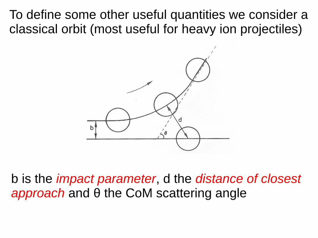
To define some other useful quantities we consider aclassical orbit (most useful for heavy ion projectiles)

b is the impact parameter, d the distance of closest approach and θ the CoM scattering angle

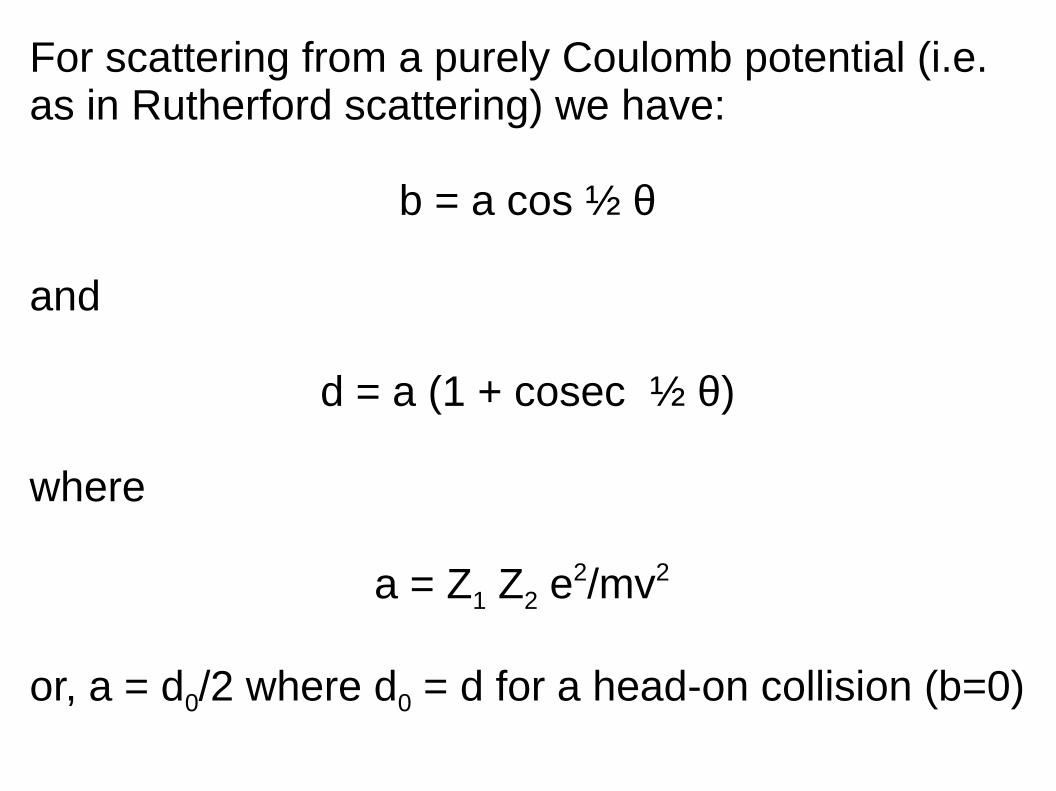
For scattering from a purely Coulomb potential (i.e.as in Rutherford scattering) we have:

b = a cos ½ θ

and

d = a (1 + cosec ½ θ)

where

a = Z1 Z2 e2/mv2

or, a = d0/2 where d0 = d for a head-on collision (b=0)

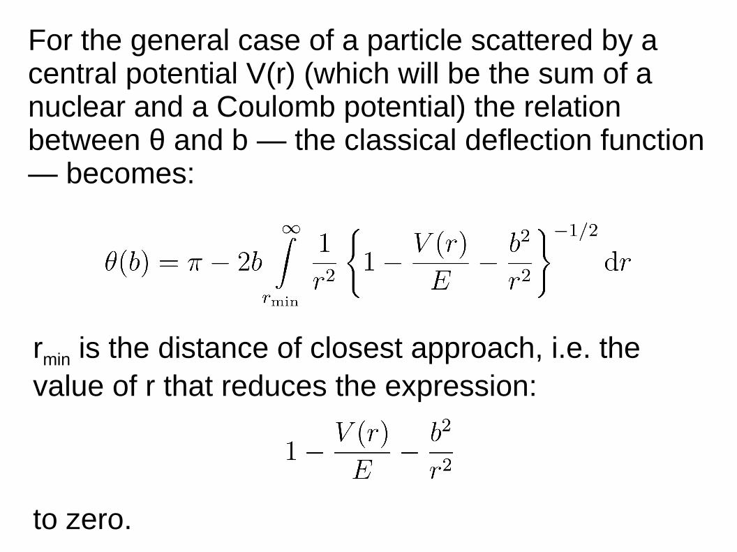
For the general case of a particle scattered by a central potential V(r) (which will be the sum of anuclear and a Coulomb potential) the relation between θ and b ― the classical deflection function― becomes:

rmin is the distance of closest approach, i.e. the value of r that reduces the expression:

to zero.

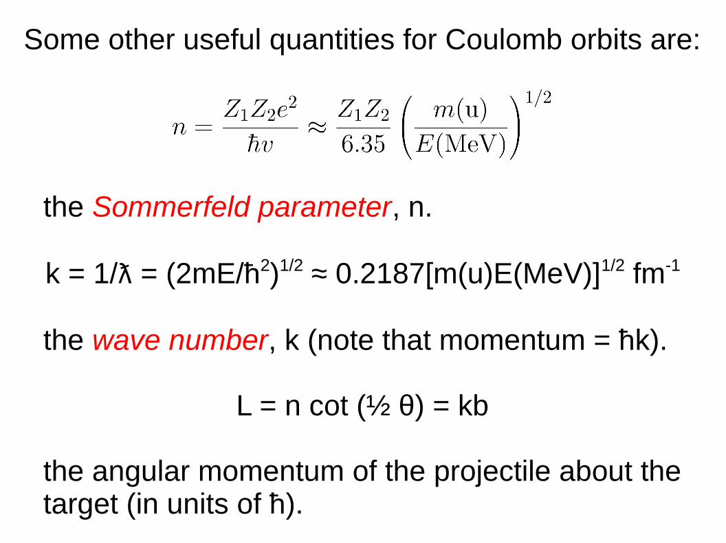
Some other useful quantities for Coulomb orbits are:

the Sommerfeld parameter, n.

k = 1/ƛ = (2mE/ħ2)1/2 ≈ 0.2187[m(u)E(MeV)]1/2 fm-1

the wave number, k (note that momentum = ħk).

L = n cot (½ θ) = kb

the angular momentum of the projectile about thetarget (in units of ħ).

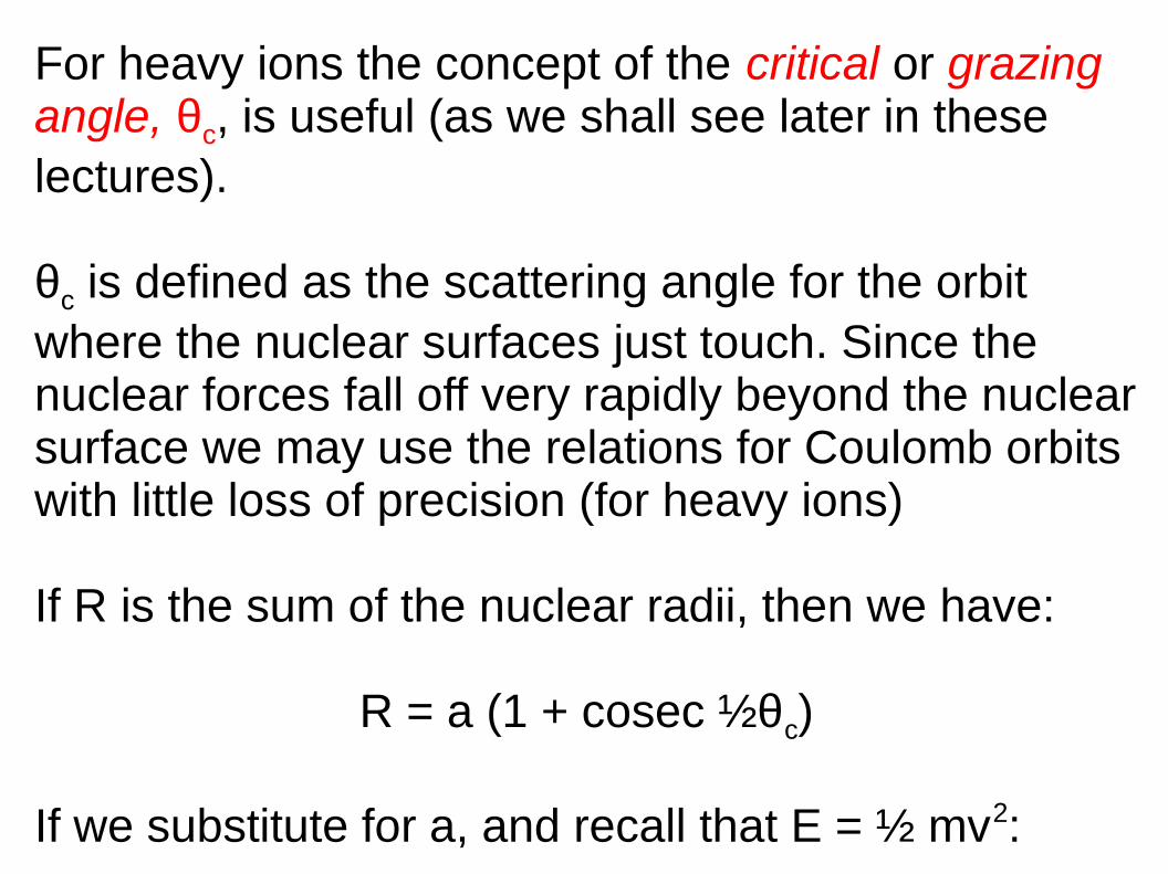
For heavy ions the concept of the critical or grazingangle, θc, is useful (as we shall see later in theselectures).

θc is defined as the scattering angle for the orbitwhere the nuclear surfaces just touch. Since the nuclear forces fall off very rapidly beyond the nuclearsurface we may use the relations for Coulomb orbitswith little loss of precision (for heavy ions)

If R is the sum of the nuclear radii, then we have:

R = a (1 + cosec ½θc)

If we substitute for a, and recall that E = ½ mv2:

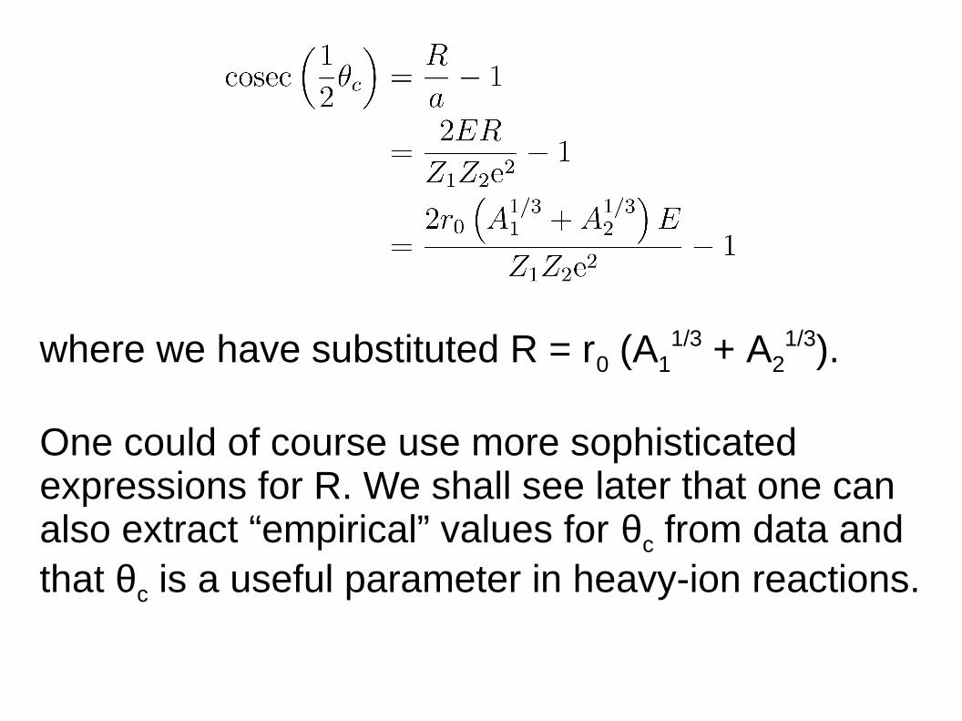
where we have substituted R = r0 (A11/3 + A2

1/3).

One could of course use more sophisticated expressions for R. We shall see later that one canalso extract “empirical” values for θc from data andthat θc is a useful parameter in heavy-ion reactions.

All these definitions are based on classical concepts.This is a reasonable approximation provided that:

n >> 1

This condition is often satisfied for heavy ions (particularly at low energies) because they are massive and carry large charges.

We can further refine these ideas to include somequantum concepts and produce semi-classicaltheories. Some of these concepts are nevertheless useful even for light-ion induced reactions …

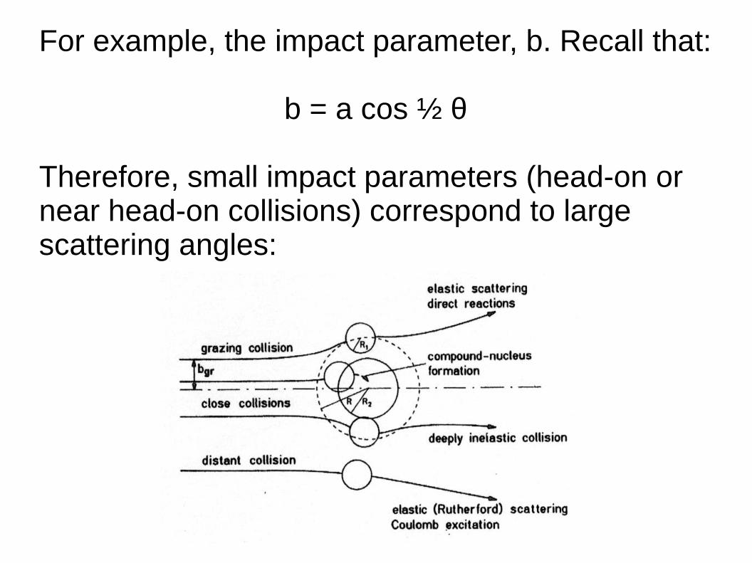
For example, the impact parameter, b. Recall that:

b = a cos ½ θ

Therefore, small impact parameters (head-on ornear head-on collisions) correspond to large scattering angles:

Lecture 2: Scattering theory

The full quantum mechanical treatment of scattering.The classical and semi-classical treatments have their uses (as we have just seen) but we need to cover the essentials of the quantum mechanical theory heresince it underlies the analysis methods we shall describe later.

Those interested in going further are referred to thebooks by Satchler (Direct Nuclear Reactions), Austern(Direct Nuclear Reaction Theories, Wiley 1970) andGlendenning (Direct Nuclear Reactions, AcademicPress 1983 or World Scientific 2004).

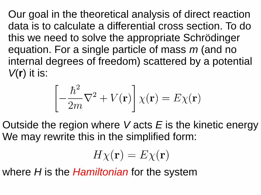
Our goal in the theoretical analysis of direct reactiondata is to calculate a differential cross section. To dothis we need to solve the appropriate Schrödingerequation. For a single particle of mass m (and nointernal degrees of freedom) scattered by a potentialV(r) it is:

Outside the region where V acts E is the kinetic energyWe may rewrite this in the simplified form:

where H is the Hamiltonian for the system

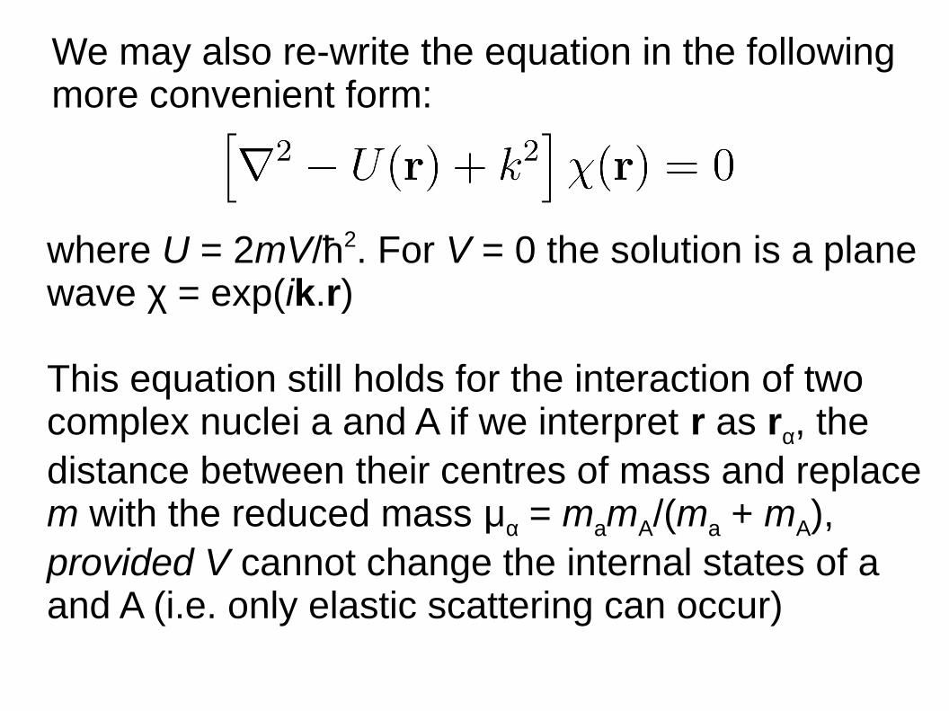
We may also re-write the equation in the followingmore convenient form:

where U = 2mV/ħ2. For V = 0 the solution is a planewave χ = exp(ik.r)

This equation still holds for the interaction of twocomplex nuclei a and A if we interpret r as rα, thedistance between their centres of mass and replacem with the reduced mass μα = mamA/(ma + mA),provided V cannot change the internal states of aand A (i.e. only elastic scattering can occur)

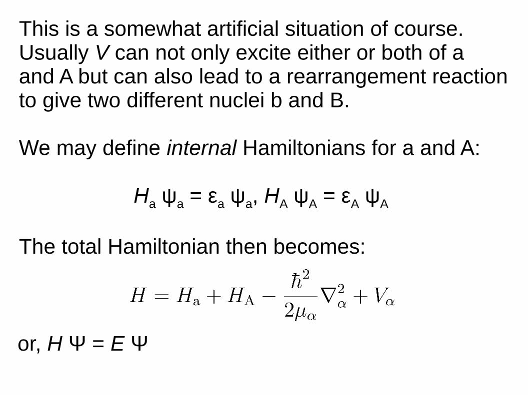
This is a somewhat artificial situation of course. Usually V can not only excite either or both of a and A but can also lead to a rearrangement reactionto give two different nuclei b and B.

We may define internal Hamiltonians for a and A:

Ha ψa = εa ψa, HA ψA = εA ψA

The total Hamiltonian then becomes:

or, H Ψ = E Ψ

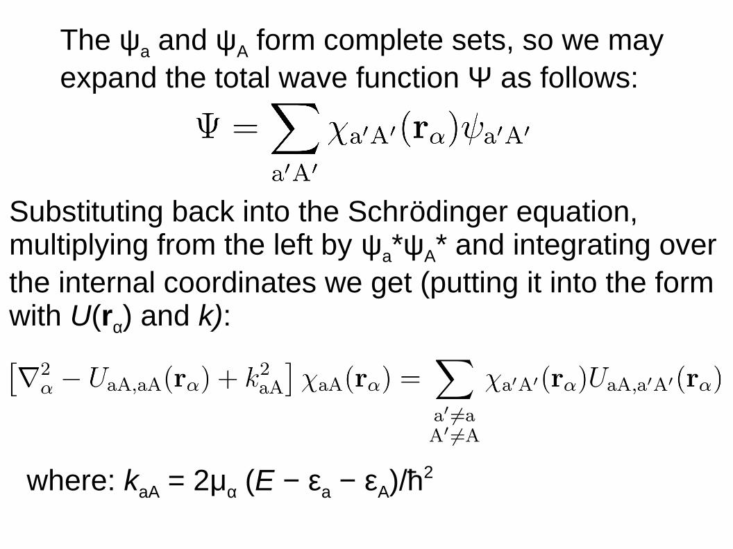
The ψa and ψA form complete sets, so we may expand the total wave function Ψ as follows:

Substituting back into the Schrödinger equation,multiplying from the left by ψa*ψA* and integrating overthe internal coordinates we get (putting it into the form with U(rα) and k):

where: kaA = 2μα (E − εa − εA)/ħ2

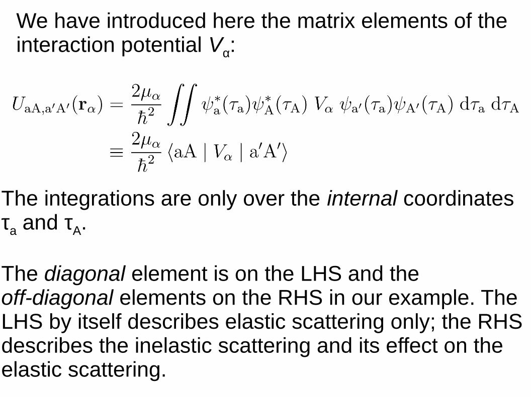
We have introduced here the matrix elements of the interaction potential Vα:

The integrations are only over the internal coordinates τa and τA.

The diagonal element is on the LHS and the off-diagonal elements on the RHS in our example. The LHS by itself describes elastic scattering only; the RHS describes the inelastic scattering and its effect on the elastic scattering.

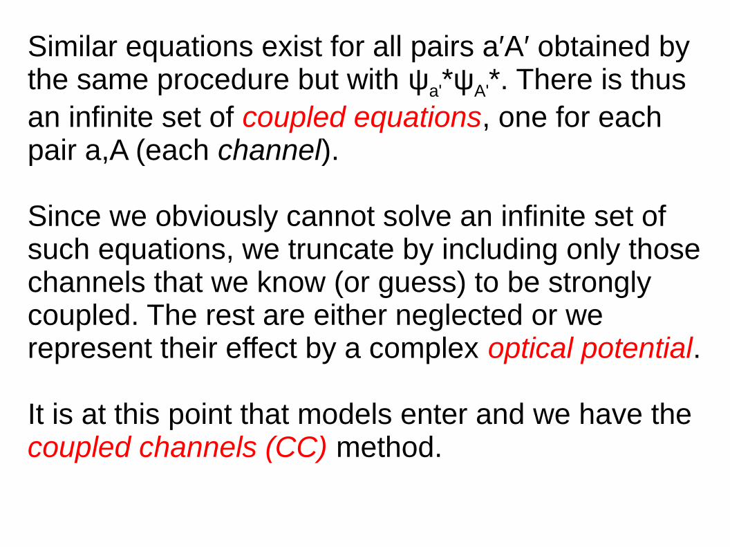
Similar equations exist for all pairs a′A′ obtained by the same procedure but with ψa'*ψA'*. There is thusan infinite set of coupled equations, one for eachpair a,A (each channel).

Since we obviously cannot solve an infinite set ofsuch equations, we truncate by including only thosechannels that we know (or guess) to be stronglycoupled. The rest are either neglected or we represent their effect by a complex optical potential.

It is at this point that models enter and we have thecoupled channels (CC) method.

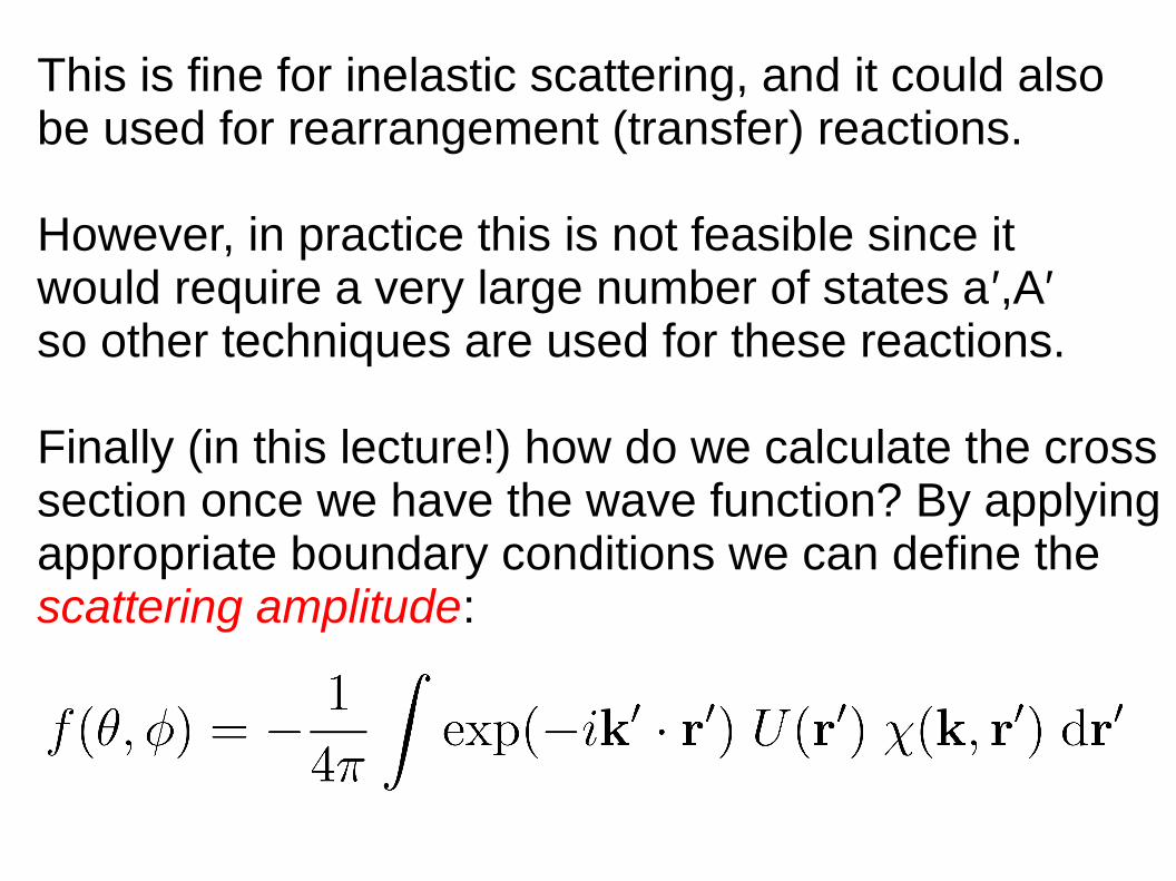
This is fine for inelastic scattering, and it could also be used for rearrangement (transfer) reactions.

However, in practice this is not feasible since itwould require a very large number of states a′,A′so other techniques are used for these reactions.

Finally (in this lecture!) how do we calculate the crosssection once we have the wave function? By applyingappropriate boundary conditions we can define thescattering amplitude:

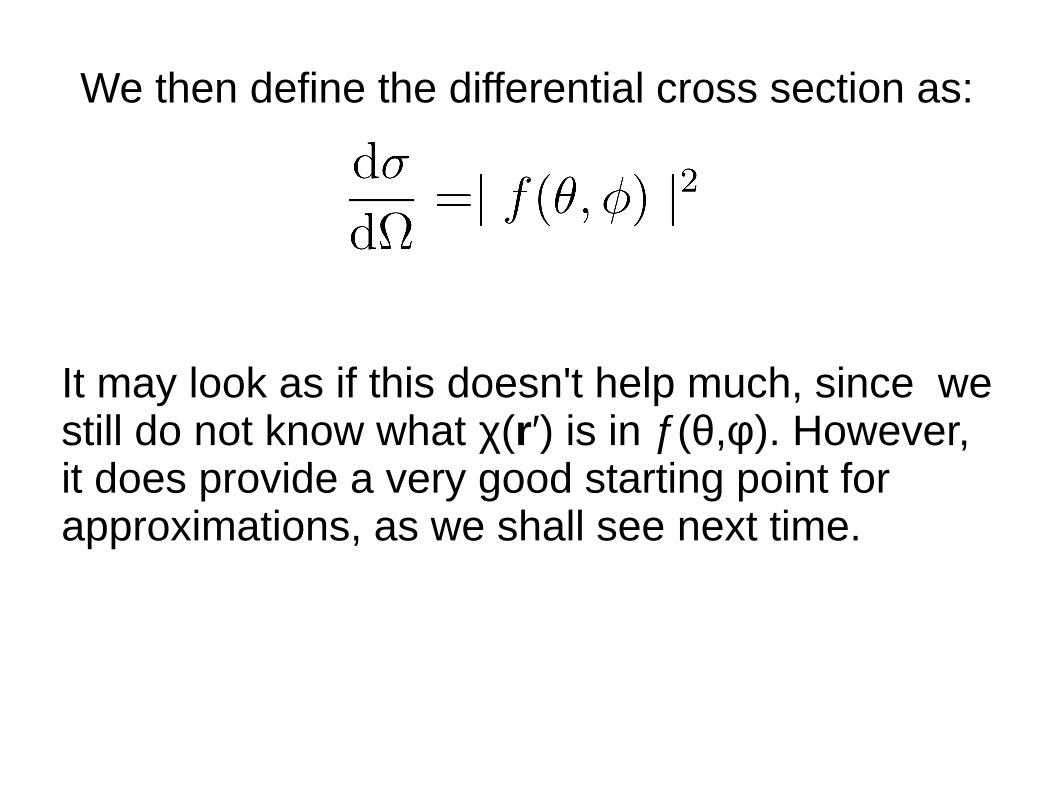
We then define the differential cross section as:

It may look as if this doesn't help much, since westill do not know what χ(r′) is in ƒ(θ,φ). However, it does provide a very good starting point forapproximations, as we shall see next time.

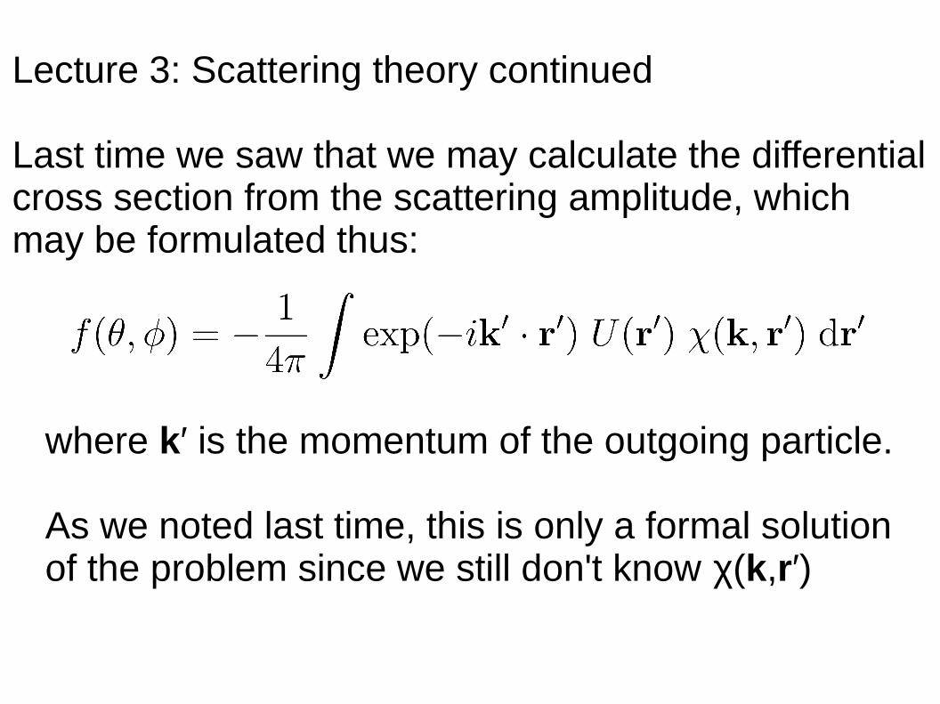
Lecture 3: Scattering theory continued

Last time we saw that we may calculate the differentialcross section from the scattering amplitude, which may be formulated thus:

where k′ is the momentum of the outgoing particle.

As we noted last time, this is only a formal solutionof the problem since we still don't know χ(k,r′)

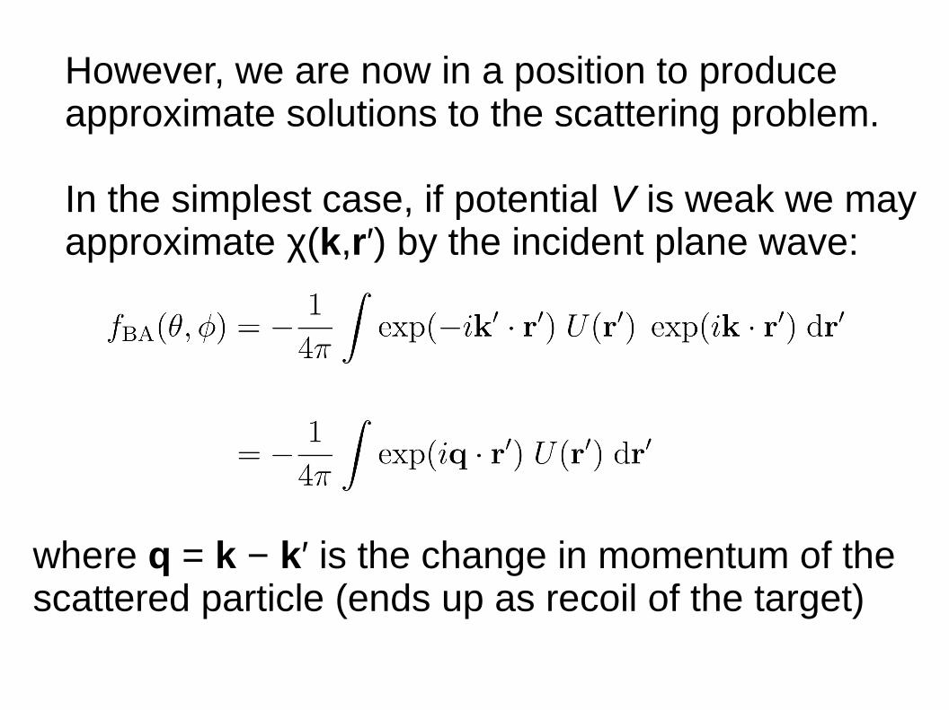
However, we are now in a position to produceapproximate solutions to the scattering problem.

In the simplest case, if potential V is weak we mayapproximate χ(k,r′) by the incident plane wave:

where q = k − k′ is the change in momentum of the scattered particle (ends up as recoil of the target)

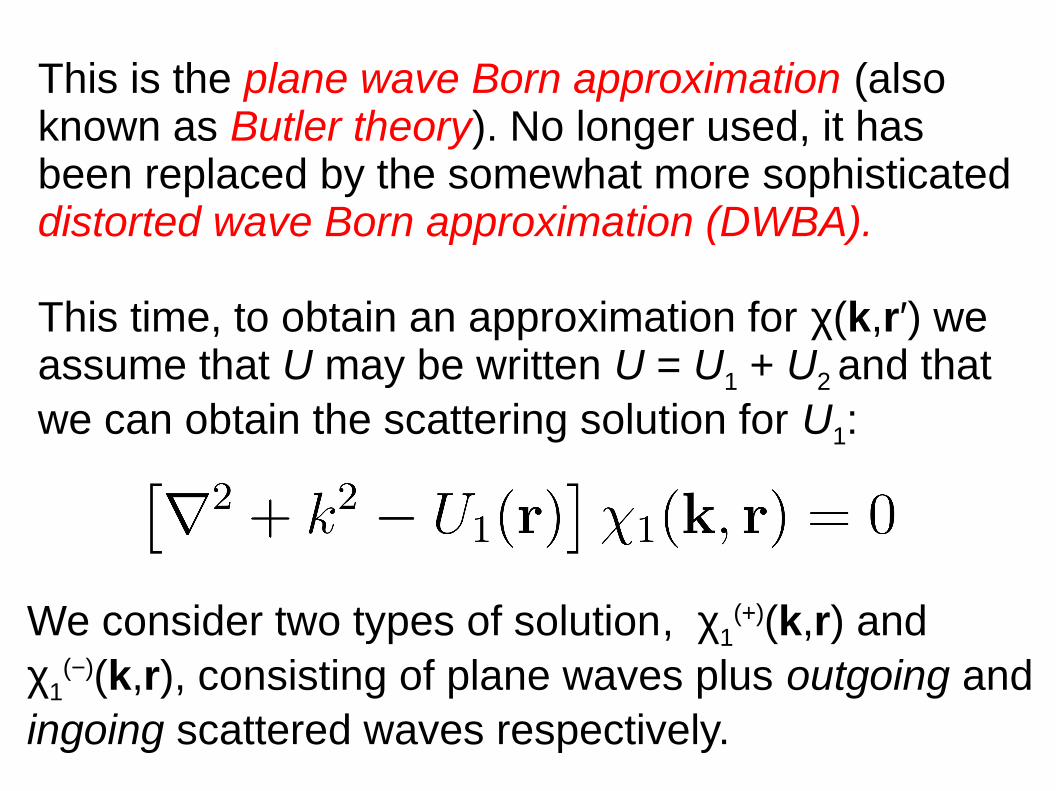
This is the plane wave Born approximation (alsoknown as Butler theory). No longer used, it hasbeen replaced by the somewhat more sophisticateddistorted wave Born approximation (DWBA).

This time, to obtain an approximation for χ(k,r′) weassume that U may be written U = U1 + U2 and thatwe can obtain the scattering solution for U1:

We consider two types of solution, χ1(+)(k,r) and

χ1(−)(k,r), consisting of plane waves plus outgoing and

ingoing scattered waves respectively.

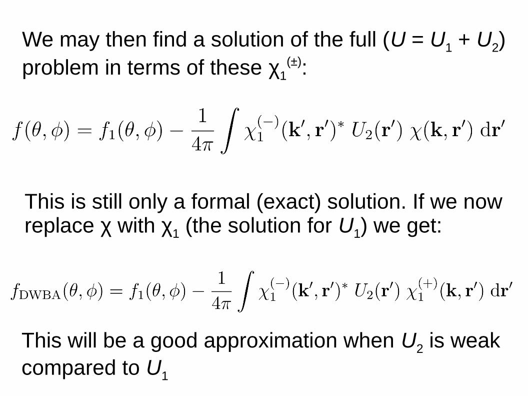
We may then find a solution of the full (U = U1 + U2)problem in terms of these χ1

(±):

This is still only a formal (exact) solution. If we nowreplace χ with χ1 (the solution for U1) we get:

This will be a good approximation when U2 is weak compared to U1

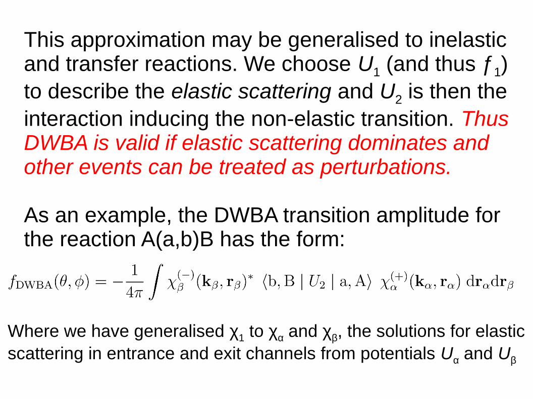
This approximation may be generalised to inelasticand transfer reactions. We choose U1 (and thus ƒ1)to describe the elastic scattering and U2 is then theinteraction inducing the non-elastic transition. ThusDWBA is valid if elastic scattering dominates andother events can be treated as perturbations.

As an example, the DWBA transition amplitude forthe reaction A(a,b)B has the form:

Where we have generalised χ1 to χα and χβ, the solutions for elasticscattering in entrance and exit channels from potentials Uα and Uβ

Finally, a few words on partial wave expansion. Therelative angular momentum of two colliding particles,ℓћ, is quantised in units of ћ. Since nuclear forces areshort ranged and nuclei have reasonably sharp edgesonly particles with angular momentum less than somemaximum value interact with the target. This can bequite small (for protons, as little as ℓ = 10 – 15).

If we have a central potential (usual in nuclear reactions) angular momentum is conserved and we may write:

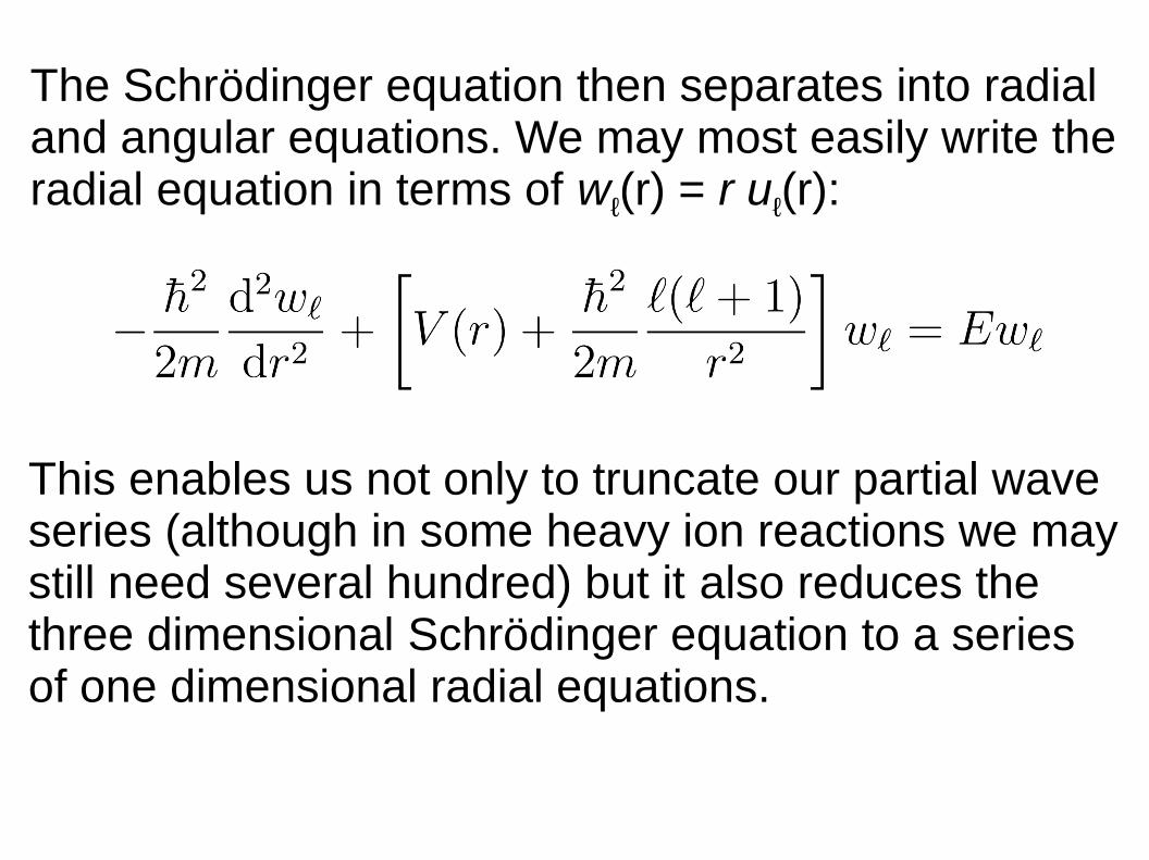
The Schrödinger equation then separates into radialand angular equations. We may most easily write theradial equation in terms of wℓ(r) = r uℓ(r):

This enables us not only to truncate our partial wave series (although in some heavy ion reactions we maystill need several hundred) but it also reduces thethree dimensional Schrödinger equation to a series of one dimensional radial equations.

Lecture 3: elastic scattering and the optical model

We now begin the main subject of these lectures: howdo we interpret direct reactions and why should westudy them?

We start with the most fundamental process, elasticscattering. It is always present, so any direct reactiontheory must take account of it in some way. Here weconsider the simplest theory of elastic scattering, theoptical model, which treats elastic scattering alone.

The optical model replaces the full scattering problemwith that for scattering by a (complex) potential, thesimplest case we considered in our brief look atscattering theory.

The optical potential must be complex to account forabsorption into other reaction channels that we donot treat explicitly.

It is possible formally to construct an optical potentialof this type from the full problem in scattering theory(usually referred to as “Feshbach Theory”). However,in practice it is virtually impossible to calculate sucha potential which is in any case non-local and L-dependent.

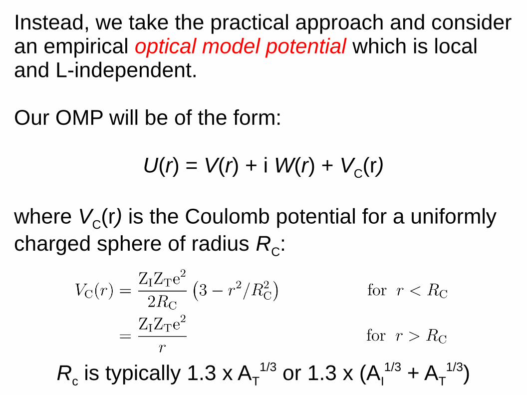
Instead, we take the practical approach and consideran empirical optical model potential which is localand L-independent.

Our OMP will be of the form:

U(r) = V(r) + i W(r) + VC(r)

where VC(r) is the Coulomb potential for a uniformlycharged sphere of radius RC:

Rc is typically 1.3 x AT1/3 or 1.3 x (AI

1/3 + AT1/3)

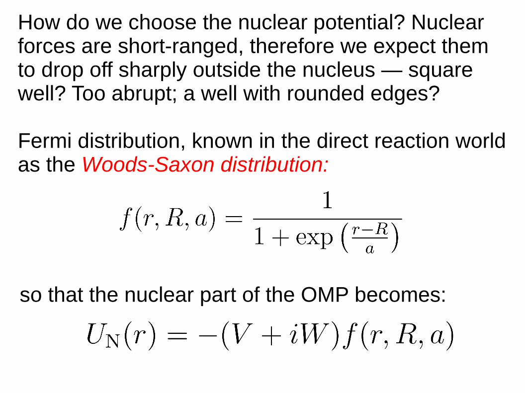
How do we choose the nuclear potential? Nuclearforces are short-ranged, therefore we expect themto drop off sharply outside the nucleus — squarewell? Too abrupt; a well with rounded edges?

Fermi distribution, known in the direct reaction worldas the Woods-Saxon distribution:

so that the nuclear part of the OMP becomes:

In this form we have four adjustable parameters:V, W, R and a. However, there is no a priori reason why R and a need be the same for the real and imaginary parts of the potential, so we can have up to six parameters to be determined.

This is the usual form employed in analyses ofheavy ion elastic scattering data. However, it isnormally found that only three parameters need bevaried (for a given system): V, W and aW (more onthis later).

For nucleons and other light ions we usually go alittle further:

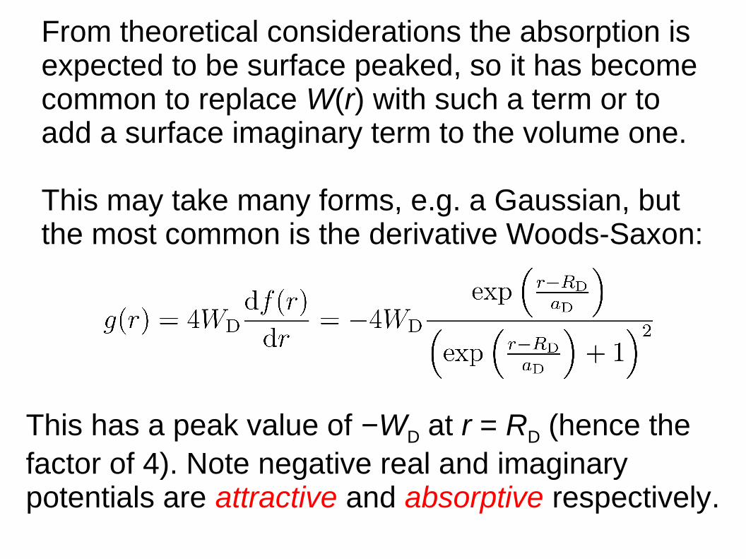
From theoretical considerations the absorption isexpected to be surface peaked, so it has becomecommon to replace W(r) with such a term or toadd a surface imaginary term to the volume one.

This may take many forms, e.g. a Gaussian, butthe most common is the derivative Woods-Saxon:

This has a peak value of −WD at r = RD (hence the factor of 4). Note negative real and imaginary potentials are attractive and absorptive respectively.

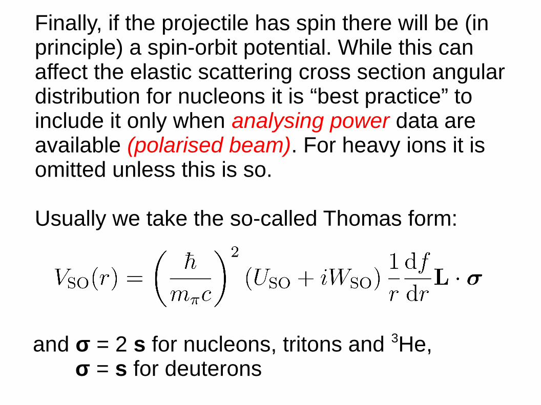
Finally, if the projectile has spin there will be (inprinciple) a spin-orbit potential. While this canaffect the elastic scattering cross section angulardistribution for nucleons it is “best practice” toinclude it only when analysing power data areavailable (polarised beam). For heavy ions it isomitted unless this is so.

Usually we take the so-called Thomas form:

and σ = 2 s for nucleons, tritons and 3He, σ = s for deuterons

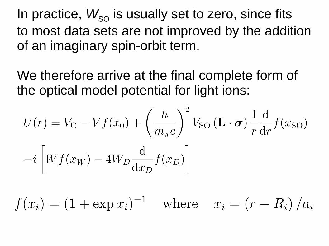
In practice, WSO is usually set to zero, since fits to most data sets are not improved by the additionof an imaginary spin-orbit term.

We therefore arrive at the final complete form ofthe optical model potential for light ions:

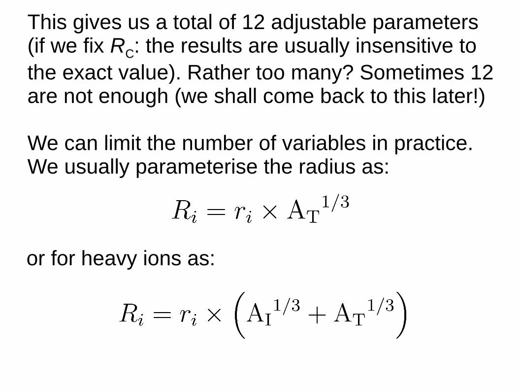
This gives us a total of 12 adjustable parameters(if we fix RC: the results are usually insensitive to the exact value). Rather too many? Sometimes 12are not enough (we shall come back to this later!)

We can limit the number of variables in practice.We usually parameterise the radius as:

or for heavy ions as:

This removes the “trivial” dependence on mass number and we can often fix the ri for a wide rangeof nuclei (so although in principle r0, rW, rD and rSO

could all have different values they remain fixed).“Typical” values for nucleons are ri = 1.15 fm or1.25 fm. Often r0 and rSO will be fixed at the samevalue, with rW and rD fixed at a different value.

It has been found from a large number of analysesthat the OMP parameters for a given projectile +target combination vary as a function of bombardingenergy. This is true for both nucleons and other lightions and heavy ions, although it can be difficult toprove this for the latter.

The reasons are, however, different. Recall that theformal optical potential is both non-local and L-dependent. While it is always possible to find alocal equivalent to such a potential (with someconsequences that we will come back to when welook at transfer reactions) this introduces an energydependence into the local equivalent potential.

For nucleons this energy dependence is dominatedby the non-locality introduced by exchange effects.

For heavy ions, exchange effects are essentiallynegligible, and the energy dependence in the localequivalent potential is due to the non-locality inducedby couplings to other reaction channels.

It should be remembered that the empirical OMP that we obtain by fitting data is not the “local equivalent”of the formal optical potential but a purely empiricalobject, so that some of the energy dependence ofthe parameters that we find may be intrinsic ratherthan a consequence of the two sources of non-locality

To recap, we have seen that in its full form the empirical OMP may have up to 12 adjustable parameters. Supposing that we are able to obtain agood description of data by adjusting these parameters (we shall briefly explain how this is donein the next lecture) what have we gained by so doing?

1) By fitting large numbers of data sets for many systems over a wide range of energies we can look for systematic variations with A, Z and incident energy (cf. Kepler and Tycho Brahe's planetary observations).

2) For light ions (particularly nucleons) we may obtain “global” parameter sets that fit in an average way large bodies of data for different systems. These are useful in many ways, but can provide greatest insight when they fail badly — this can be an indication of shell effects etc.

3) They are needed as input to other calculations (inelastic scattering and transfer reactions).

It would, of course, be much more satisfying if wecould calculate an optical model potential from firstprinciples. We have said that trying to do so usingFeshbach theory is virtually impossible. However,it has been done — with considerable success —for nucleons.

While there are more modern theories, the standardto which these are compared is the so-called “JLM”potential: J. P. Jeukenne, A. Lejeune, and C. Mahaux, Phys. Rev. C 16, 80 (1977). This approach is based on a complex effective nucleon-nucleon interaction and infinite nuclear matter (folded over the target density) so works less well for light targets.

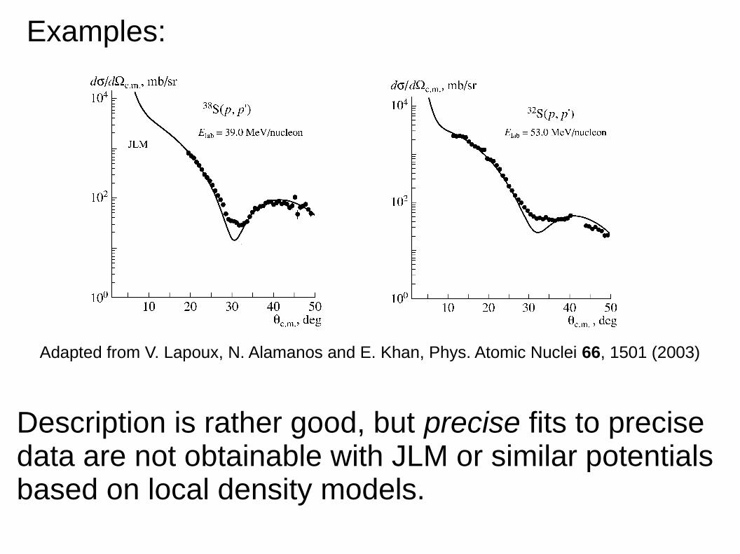
Examples:

Adapted from V. Lapoux, N. Alamanos and E. Khan, Phys. Atomic Nuclei 66, 1501 (2003)

Description is rather good, but precise fits to precisedata are not obtainable with JLM or similar potentialsbased on local density models.

For heavy ions, although various attempts have beenmade to calculate an OMP the agreement with datais usually worse. The problem is in calculating theimaginary part of the potential. As we shall see later,the real part may be calculated with considerablesuccess for heavy ions, based on clues given by theformal theory.

In the next lecture we shall examine how the opticalmodel is used in practice to analyse light ion elasticscattering data.

Lecture 4: Optical model analysis of light ion elasticscattering

Before proceeding to show how an optical modelanalysis is performed in practice we will make a few general observations about how light ion elasticscattering data are presented.

Very often, proton elastic scattering data are plottedon an absolute cross section scale, i.e. the angulardistribution of the differential cross section isplotted in units of mb/sr:

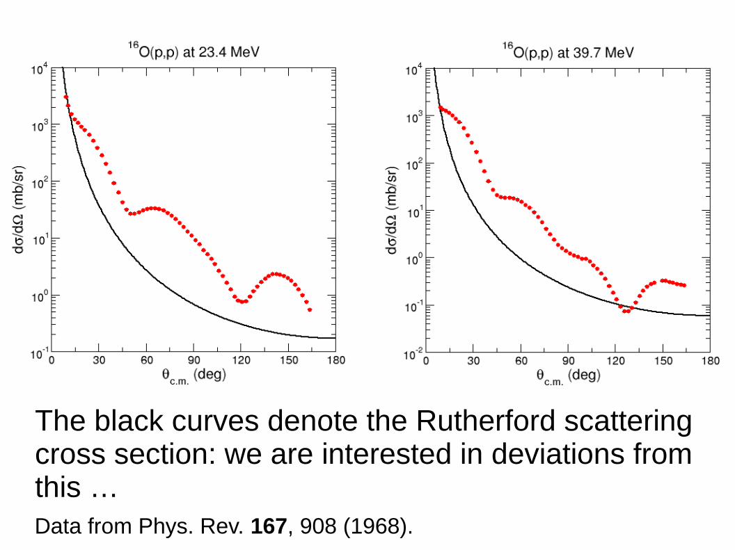
The black curves denote the Rutherford scatteringcross section: we are interested in deviations fromthis …Data from Phys. Rev. 167, 908 (1968).

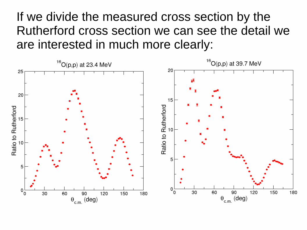
If we divide the measured cross section by theRutherford cross section we can see the detail weare interested in much more clearly:

This is not usually done for proton scattering, but it should be! It is, however, fairly routine for plotting theelastic scattering of deuterons or heavier ions.

Now (finally) how do we go about performing an optical model analysis?

Even for the relatively simple problem of scatteringfrom a (complex) potential well the equations haveto be solved numerically. Our first requirement isthus a code to perform the numerical calculations.

Several are available: ECIS, FRESCO (SFRESCO),HERMES. All allow searching on parameters (weshall return to this shortly).

ECIS and FRESCO are general direct reaction codeswhich of course includes the ability to perform optical model calculations. HERMES is a specific optical model code. DWBA codes such as DWUCK can also calculate the elastic scattering using the optical model but do not usually allow parameter searches.

Optical model calculations have to be performednumerically (there are no analytic solutions). However, the asymptotic solutions for the wave function are known analytically, so we may save some trouble by matching to these at an appropriate radius, the matching radius, Rm.

We also need to define a radial step size for thenumerical integrations that have to be performed, dr.

Finally, we truncate the infinite series of partial wavesat some finite number, ℓmax.

How do we choose these numbers for a particularcase? There is a useful “rule of thumb” which uses the relationship between ℓ and Rℓ, the classical turning point of the Rutherford orbit:

ℓ (ℓ + 1) = kRℓ (kRℓ − 2n)

k = 0.2187[m(u)E(MeV)]1/2 fm-1

n = 0.1575 Z1Z2[m(u)/E(MeV)]1/2

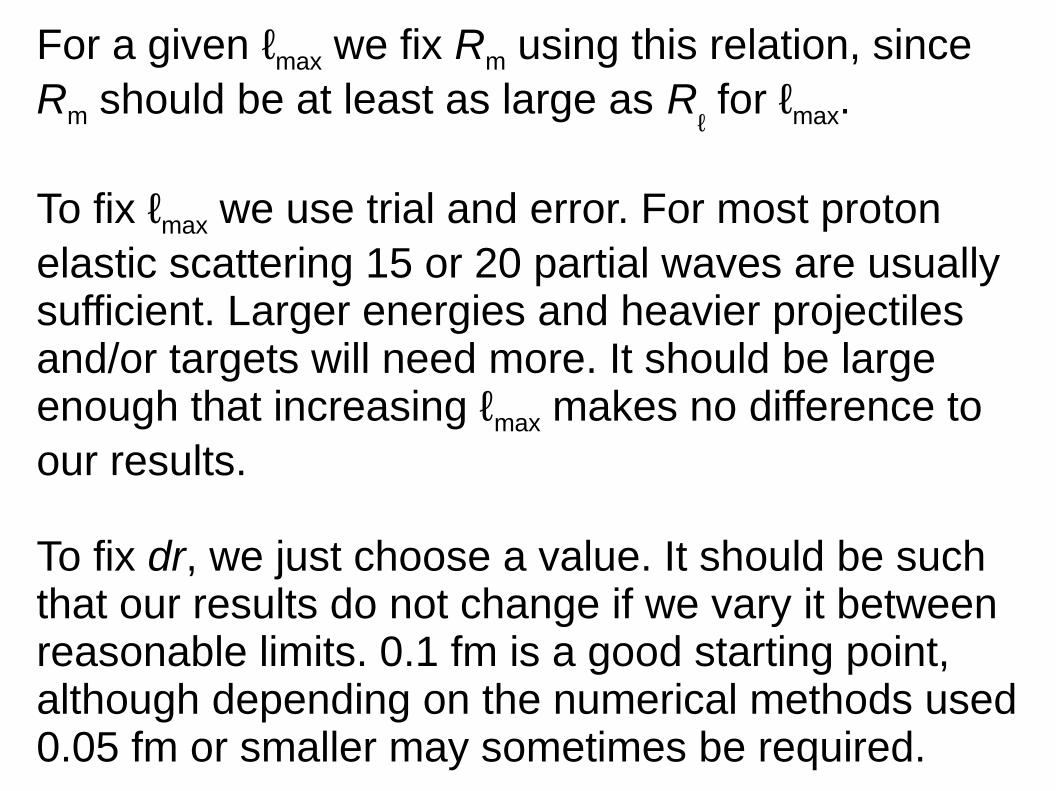
For a given ℓmax we fix Rm using this relation, since Rm should be at least as large as R

ℓ for ℓmax.

To fix ℓmax we use trial and error. For most protonelastic scattering 15 or 20 partial waves are usuallysufficient. Larger energies and heavier projectilesand/or targets will need more. It should be largeenough that increasing ℓmax makes no difference toour results.

To fix dr, we just choose a value. It should be such that our results do not change if we vary it betweenreasonable limits. 0.1 fm is a good starting point,although depending on the numerical methods used0.05 fm or smaller may sometimes be required.

As an example we consider the 16O(p,p) data wesaw earlier. There exists in the literature a set ofpotentials for these data in Phys. Rev. 184, 1061 (1969), so we begin by repeating these calculations.We use the code FRESCO (www.fresco.org.uk)

Points to watch in this type of exercise:

1) Check the definition of any surface terms with that used in the code of your choice. In this case there is a surface imaginary term of Gaussian form. The same thing applies to any spin-orbit terms; sometimes L . s is used rather than L . σ

2) Do a visual check of the calculation compared to the data; does your calculation match the original? Also check the value of the reaction cross section, if given. Does it match your value? (within small variations due to machine precision).

Now we choose the parameters for the numericalevaluation. Start with dr = 0.1 fm. We take ℓmax = 15as a starting point, which gives values of 15.8 fmand 12.1 fm for the classical turning points at 23.4and 39.7 MeV respectively. Take R

m = 16 and 15 fm.

How do the results compare to the original calculations and the data?

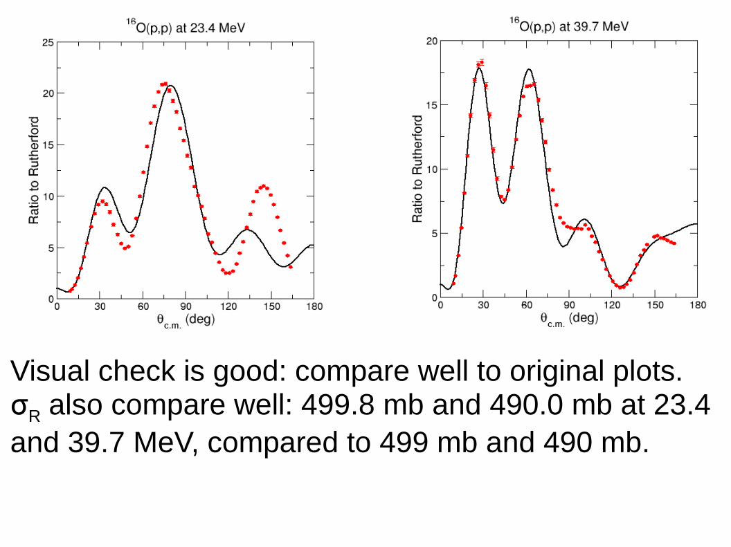
Visual check is good: compare well to original plots.σR also compare well: 499.8 mb and 490.0 mb at 23.4 and 39.7 MeV, compared to 499 mb and 490 mb.

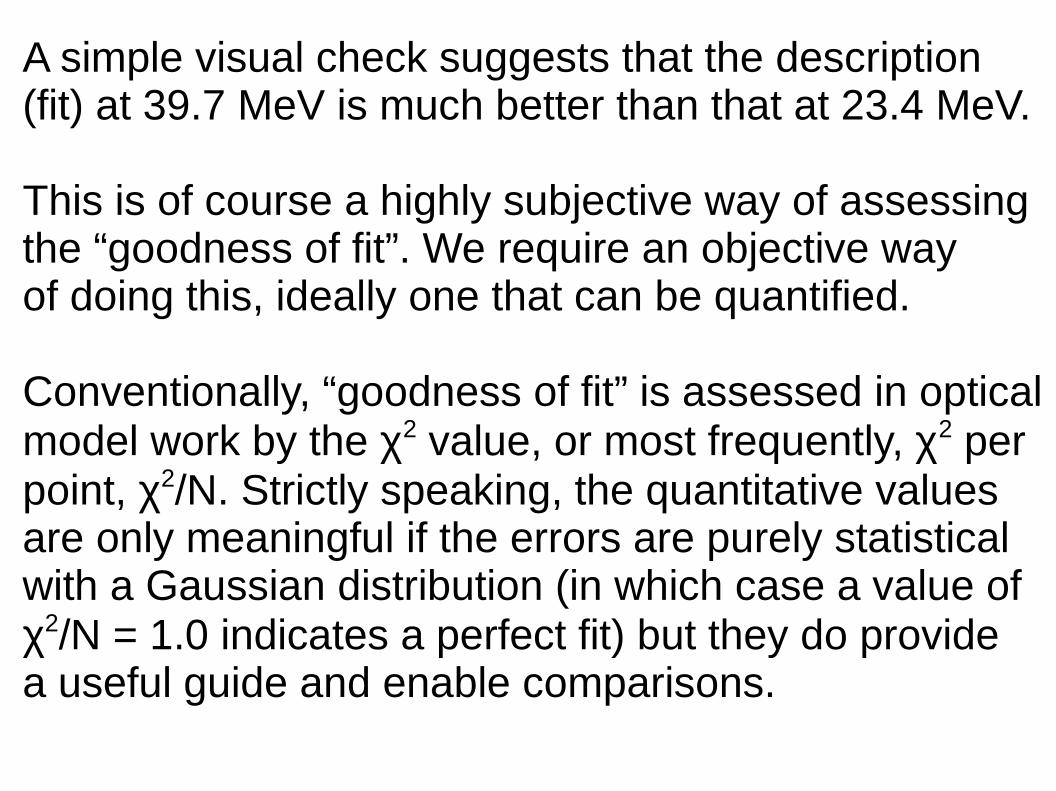
A simple visual check suggests that the description(fit) at 39.7 MeV is much better than that at 23.4 MeV.

This is of course a highly subjective way of assessingthe “goodness of fit”. We require an objective wayof doing this, ideally one that can be quantified.

Conventionally, “goodness of fit” is assessed in opticalmodel work by the χ2 value, or most frequently, χ2 perpoint, χ2/N. Strictly speaking, the quantitative valuesare only meaningful if the errors are purely statisticalwith a Gaussian distribution (in which case a value ofχ2/N = 1.0 indicates a perfect fit) but they do providea useful guide and enable comparisons.

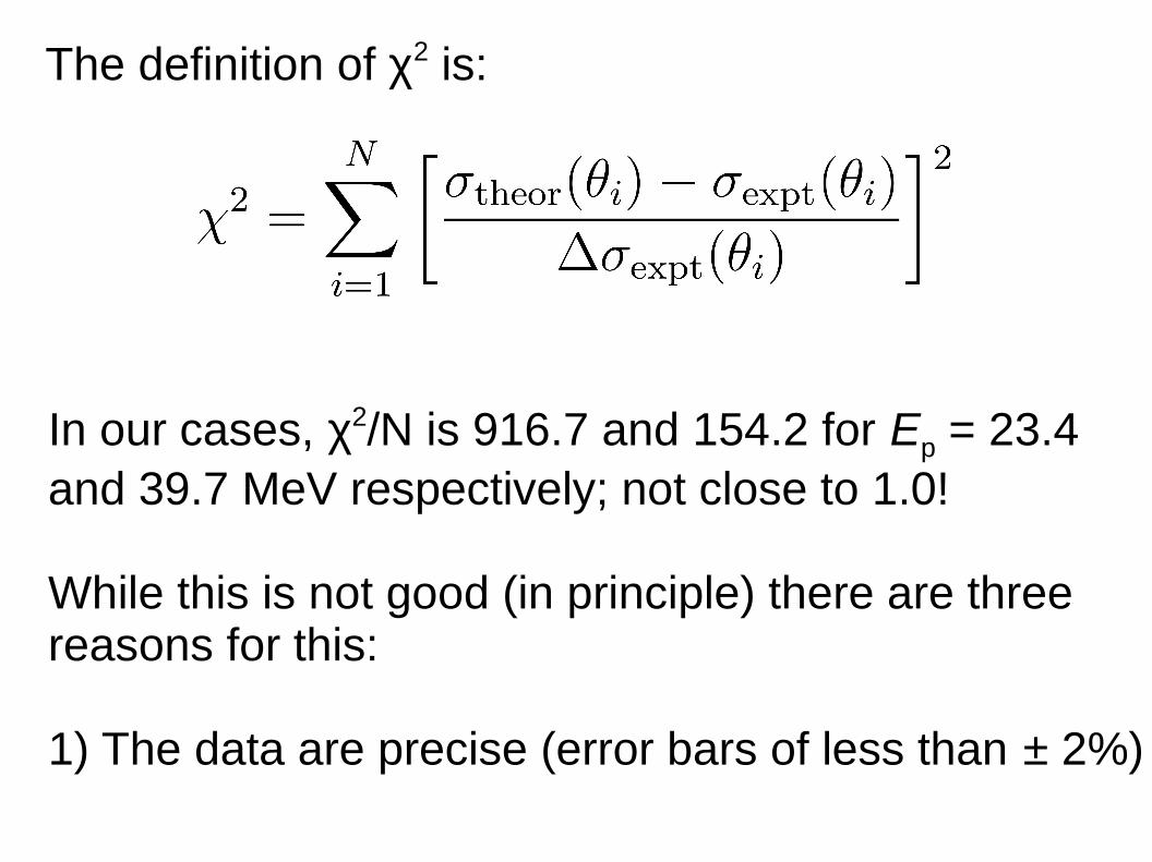
The definition of χ2 is:

In our cases, χ2/N is 916.7 and 154.2 for Ep = 23.4and 39.7 MeV respectively; not close to 1.0!

While this is not good (in principle) there are threereasons for this:

1) The data are precise (error bars of less than ± 2%)

2) The original fits were constrained to have the same “geometry” (i.e. radii and diffuseness) at all energies

3) Polarisation data were also included in the fit

However, precise data deserve precise fits; if notthere is information contained in them that we aremissing. Can we improve on these fits, and howdo we go about it?

We must search on the parameters and try tominimise χ2. However, the OMP used here has9 parameters (12 at 39.7 MeV); searching on all of them at once is not a good idea!

Two reasons:

1) Purely practical; can take a long time to minimise χ2 when varying so many parameters

2) The parameters are not, in fact, independent, there are correlations between some of them.

It is also not usually a good idea to adjust the spin-orbit potential parameters without polarisationdata.

We will see if we can improve significantly the fitat 23.4 MeV. Since the “geometry” was fixed fora wide range of energies, try searching on that.

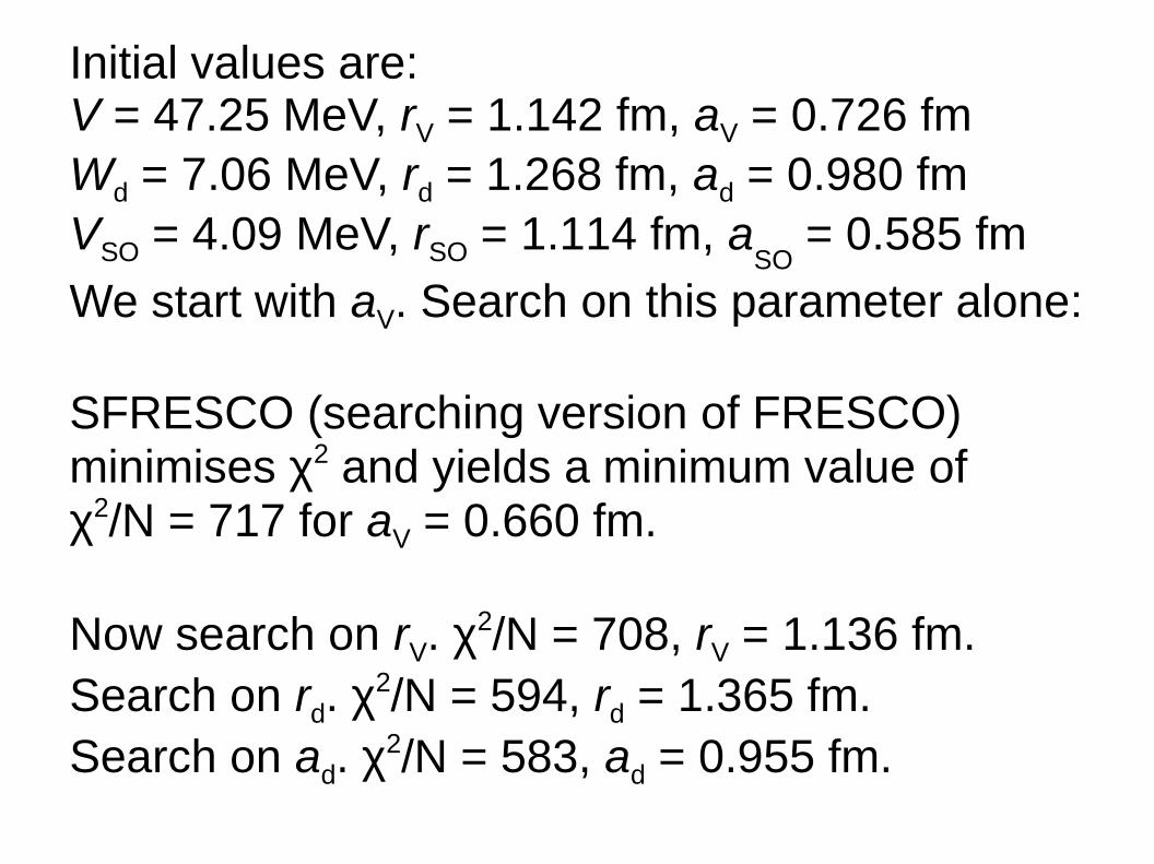
Initial values are:V = 47.25 MeV, rV = 1.142 fm, aV = 0.726 fmWd = 7.06 MeV, rd = 1.268 fm, ad = 0.980 fmVSO = 4.09 MeV, rSO = 1.114 fm, a

SO = 0.585 fm

We start with aV. Search on this parameter alone:

SFRESCO (searching version of FRESCO)minimises χ2 and yields a minimum value of χ2/N = 717 for aV = 0.660 fm.

Now search on rV. χ2/N = 708, rV = 1.136 fm.

Search on rd. χ2/N = 594, rd = 1.365 fm.

Search on ad. χ2/N = 583, ad = 0.955 fm.

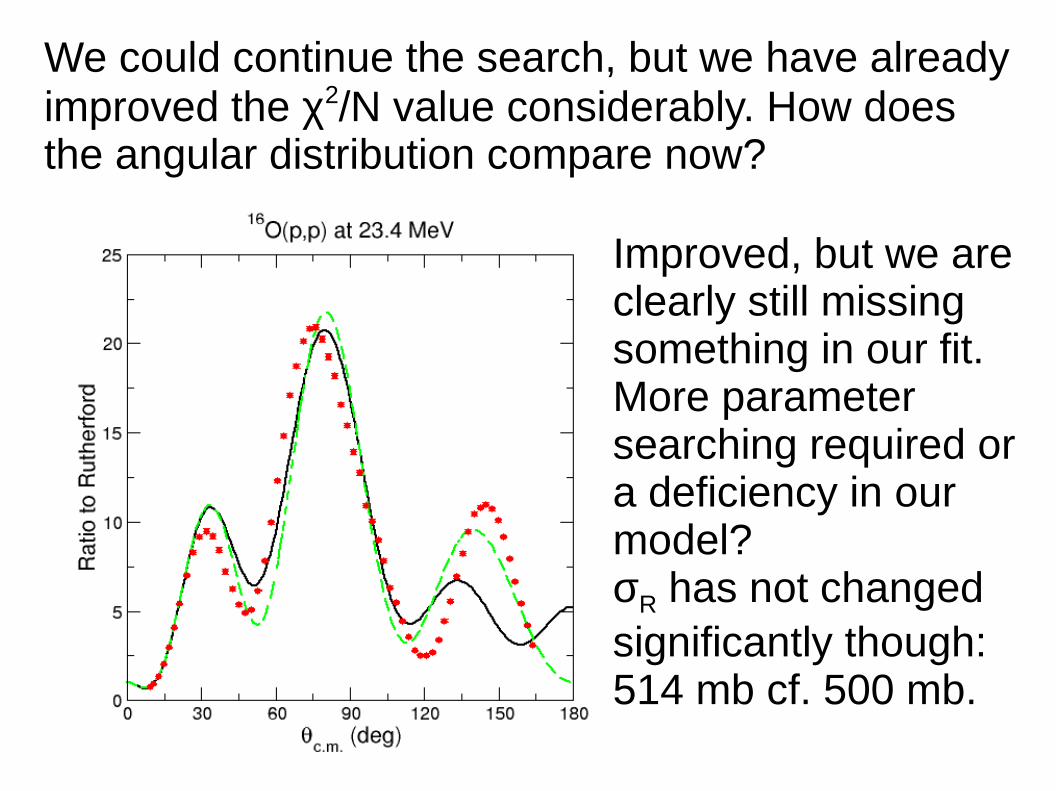
We could continue the search, but we have alreadyimproved the χ2/N value considerably. How doesthe angular distribution compare now?

Improved, but we areclearly still missingsomething in our fit.More parametersearching required ora deficiency in ourmodel?σR has not changedsignificantly though: 514 mb cf. 500 mb.

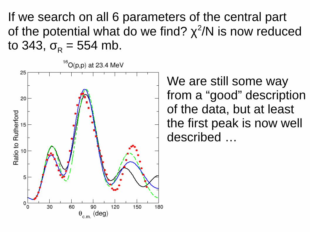
If we search on all 6 parameters of the central partof the potential what do we find? χ2/N is now reducedto 343, σR = 554 mb.

We are still some wayfrom a “good” descriptionof the data, but at leastthe first peak is now welldescribed …

Agreement is better, but parameters are now a little strained:

V = 64.65 MeV, rV = 0.9095 fm, aV = 0.841 fmWd = 6.55 MeV, rd = 1.363 fm, ad = 1.095 fm

(recall that we have not searched on spin-orbitpotential).

This is about as far as we can go without introducingyet more parameters (we could add a volume absorption term, as at 39.7 MeV, but recall the wellknown quote of von Neumann!). What does thiscomparative failure to fit the data well tell us?

1) Fitting precise data precisely can be difficult!

2) As we saw previously, the OMP is intrinsically non-local (and L-dependent). While it is always possible to find a local equivalent to this N-L potential it may not be (and in general will not be) parameterisable with “standard” potential forms.

3) Linked to 2), strong couplings may induce effective potentials that cannot be satisfactorily modelled with standard potential forms.

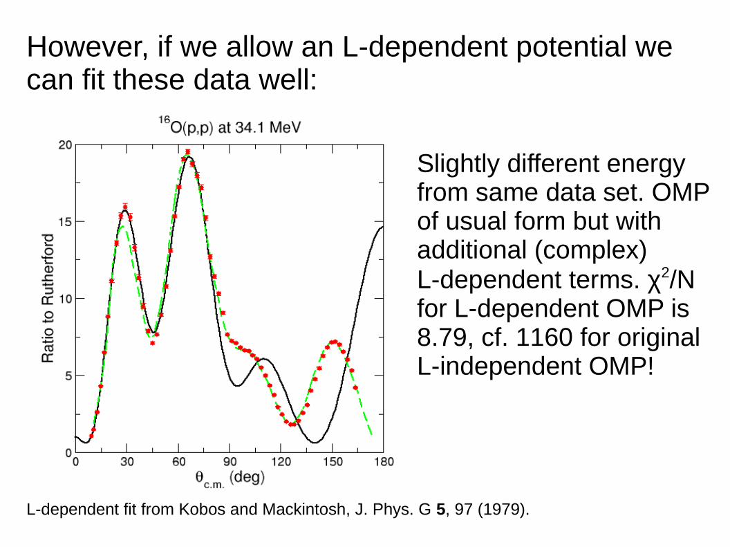
However, if we allow an L-dependent potential wecan fit these data well:

L-dependent fit from Kobos and Mackintosh, J. Phys. G 5, 97 (1979).

Slightly different energyfrom same data set. OMPof usual form but withadditional (complex)L-dependent terms. χ2/Nfor L-dependent OMP is8.79, cf. 1160 for originalL-independent OMP!

Evidence for L-dependence seems compelling. Itdoes introduce extra parameters, but improvementin quality of fit is dramatic.

The good fit does not tell us what causes the L-dependence, but at least we now know that the OMP for this system must have this characteristic.

Also suggests that standard OMP forms can beinadequate for proton scattering from light targets. Could also be a signature of strong coupling effects on elastic scattering from other reaction channels (giant resonances, (p,d) pickup etc.)

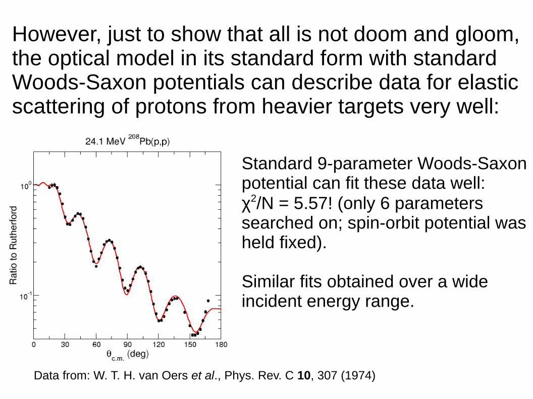
However, just to show that all is not doom and gloom,the optical model in its standard form with standardWoods-Saxon potentials can describe data for elasticscattering of protons from heavier targets very well:

Data from: W. T. H. van Oers et al., Phys. Rev. C 10, 307 (1974)

Standard 9-parameter Woods-Saxonpotential can fit these data well:χ2/N = 5.57! (only 6 parameterssearched on; spin-orbit potential washeld fixed).

Similar fits obtained over a wideincident energy range.

A word about potential ambiguities …

The OMP is not normally uniquely determined bythe data. The multi-dimensional χ2 space will ingeneral have local minima as well as the overallor “global” minimum. These minima are often quitebroad in certain directions, so some parameters arenot well determined; there are ambiguities.

OMP ambiguities are of two basic types: continuousand discrete. Continuous ambiguities arise due tothe broadness of the “valleys” or minima in the χ2

space. The best known continuous ambiguity is:

with n ≈ 2

Any change in V can be compensated for by acorresponding change in rV (within certain limits,up to about 10 %).

Similar ambiguities exist for W and aW and thereare undoubtedly more involving three parameters.

Discrete ambiguities are somewhat different. It isfound that if V is steadily increased and the otherparameters readjusted to optimise the fit χ2 passesthrough a whole series of minima. Basically, thisis due to an additional half-wave fitting inside thewell than for the next shallowest potential. Thisleads to “families” of deep and shallow potentials.

Lecture 5: Optical model analysis of heavy ion elasticscattering

While the theory we use is still the same – the opticalmodel does not differ for light and heavy ions – thereare some important differences in the analysis techniques for heavy ion elastic scattering.

The target nucleus is more or less transparent to nucleons, deuterons and to a lesser extent the other light ions (t, 3He, α).

In contrast, heavy ions are strongly absorbed andthe target is more or less opaque or even “black”.

This has important implications for optical modelanalyses: we are no longer sensitive at all to thepotential in the nuclear interior. Heavy ion elasticscattering data only determine the optical potentialin a relatively narrow region at the nuclear surfaceso that the ambiguities in the OMP extracted fromdata are even more pronounced than for light ions.

There will thus usually be many “families” of OMPsthat fit a given data set, each with its own continuousambiguities. This should always be borne in mindwhen speaking of “the OMP” for heavy ion elasticscattering.

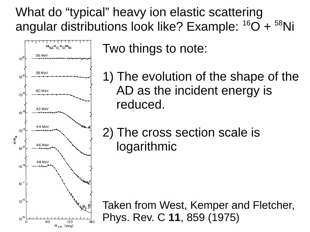
What do “typical” heavy ion elastic scatteringangular distributions look like? Example: 16O + 58Ni

Two things to note:

1) The evolution of the shape of the AD as the incident energy is reduced.

2) The cross section scale is logarithmic

Taken from West, Kemper and Fletcher, Phys. Rev. C 11, 859 (1975)

Why is the logarithmic cross section scale significant?

If we only plot our data in this fashion we may misssome significant information:

“A particularly sensitive part of the angular distribution is the oscillatory region just before the exponential fall below the Rutherford cross section. (The details of this region may be overlooked if, as is often done, the ratio-to-Rutherford cross section is shown on a semi-logarithmic plot. It is more revealing to use a linear plot.)” J. B. Ball et al., Nucl. Phys. A 252, 208 (1975).

See also: G. R. Satchler, Phys. Lett. B 55, 167 (1975).

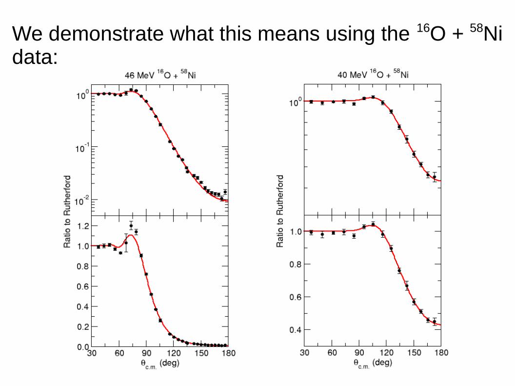
We demonstrate what this means using the 16O + 58Nidata:

Fits are from the original publication: “geometry” isfixed at r0 = 1.22 x (161/3 + 581/3) fm, a0 = 0.50 fmfor both real and imaginary parts (so vary V and Wto obtain best fit).

While the fits are rather good – χ2/N = 0.71 and 4.77at 40 and 46 MeV respectively – the linear plot showsroom for improvement at 46 MeV.

V and W are: 90.5 MeV and 7.26 MeV at 40 MeV 85.7 MeV and 33.3 MeV at 46 MeV

How well defined are these values, and how can wefind out?

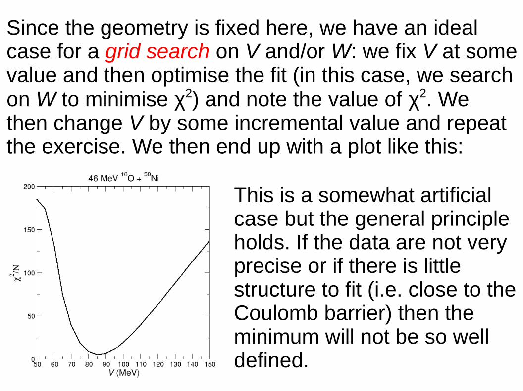
Since the geometry is fixed here, we have an idealcase for a grid search on V and/or W: we fix V at somevalue and then optimise the fit (in this case, we search on W to minimise χ2) and note the value of χ2. Wethen change V by some incremental value and repeatthe exercise. We then end up with a plot like this:

This is a somewhat artificialcase but the general principleholds. If the data are not veryprecise or if there is littlestructure to fit (i.e. close to theCoulomb barrier) then the minimum will not be so welldefined.

The constraint that the real and imaginary geometriesare the same is rather artificial for heavy ion scattering.In general it will not be possible to obtain good fits todata under this assumption (there is no real physicalreason for doing so anyway).

If we remove this constraint can we significantly improve the fit at 46 MeV ? Yes, but only at the cost of unphysical OMP parameters:

Fix rC = rV = rW = 1.3 x (161/3 + 581/3) fm

Search on the other parameters: V = 29.8 MeV, aV = 0.55 fm W = 44.4 MeV, aW = 0.324 fmχ2/N = 2.51 (c.f. previous value of 4.77)

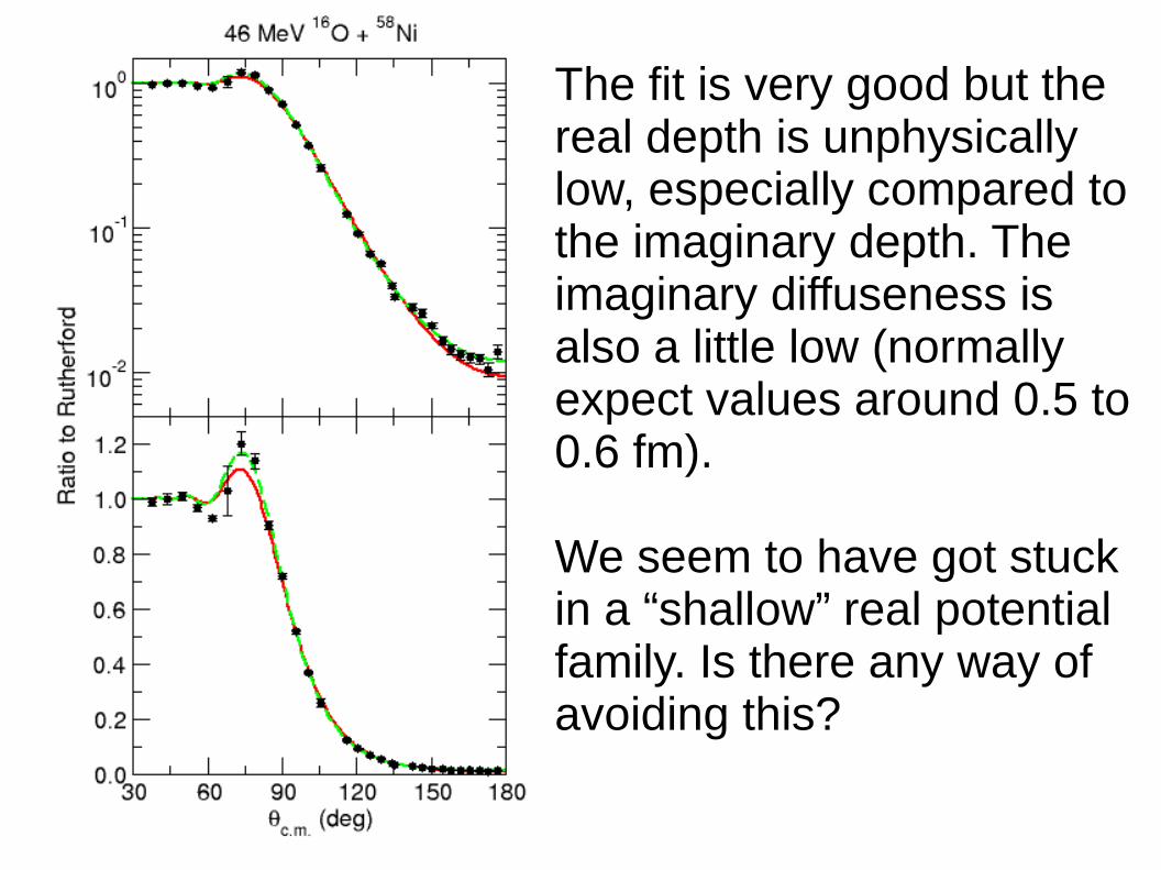
The fit is very good but thereal depth is unphysicallylow, especially compared tothe imaginary depth. Theimaginary diffuseness isalso a little low (normallyexpect values around 0.5 to0.6 fm).

We seem to have got stuckin a “shallow” real potentialfamily. Is there any way ofavoiding this?

Yes, and at the same time we can at least place the real part of the OMP on a sounder theoretical basis.

Feshbach theory gives us a clue. This suggests thatwe may write the real part of the OMP in thefollowing schematic fashion:

V(r) = Vf(r) + ΔV(r)

where Vf(r) is the so-called double-folding potentialand ΔV(r) is the real part of the dynamic polarisationpotential (DPP). The double-folding potential is obtained by integrating — “folding” — an effectivenucleon-nucleon force over the matter densities ofthe projectile and target.

The DPP arises due to the effects of coupling to thenon-elastic channels (inelastic excitations, transfers).

In fact, the DPP also has an imaginary term and wecould also write W(r) in a similar schematic fashion.The imaginary part of the DPP accounts for theabsorption induced by the couplings to other directchannels, with the equivalent of Vf(r) being animaginary potential “inside” the Coulomb barrier thataccounts for absorption due to fusion.

However, the DPP is essentially impossible tocalculate ab initio, so this formal exercise does notseem to have helped us much so far.

Nevertheless, it can be turned to practical use. Wemake no attempt to calculate the imaginary part ofthe OMP from first principles and instead keep theempirical (usually Woods-Saxon) form with its threeadjustable parameters.

For the real part, we assume that ΔV(r) is small enough compared to Vf(r) that we may safely neglect it. We therefore arrive at what we might call a “semi-microscopic” OMP of the following form:

U(r) = NR Vf(r) + i W(r)

where NR is a normalisation factor.

If our assumption is good then NR should be close to1.0. A large body of data was analysed using this model by Satchler and Love, Phys. Rep. 55, 183 (1979) and they found a mean value of:

NR ≈ 1.11 ± 0.13

so the assumption seems to be valid for a wide rangeof systems (we shall discuss the exceptions later).

The use of the double-folding model to calculate thereal part of the OMP at least fixes the shape and, tosome extent, the depth of the real potential, leavingus with a maximum of 4 adjustable parameters.

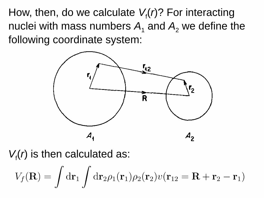
How, then, do we calculate Vf(r)? For interactingnuclei with mass numbers A1 and A2 we define thefollowing coordinate system:

Vf(r) is then calculated as:

We need the densities, ρ1(r1) and ρ2(r2) and theeffective nucleon-nucleon interaction. The densitiesare the nuclear matter densities. These can beobtained by calculation, e.g. the shell model, or canbe derived from empirical charge densities (from e.g.electron scattering).

The charge density is first converted to the protondensity by unfolding the proton charge distribution.The neutron matter density is then obtained byassuming that:

ρn = (N/Z) ρp

this is only a reasonable approximation if N ≈ Z

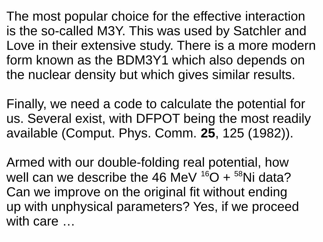
The most popular choice for the effective interactionis the so-called M3Y. This was used by Satchler andLove in their extensive study. There is a more modernform known as the BDM3Y1 which also depends onthe nuclear density but which gives similar results.

Finally, we need a code to calculate the potential forus. Several exist, with DFPOT being the most readilyavailable (Comput. Phys. Comm. 25, 125 (1982)).

Armed with our double-folding real potential, how well can we describe the 46 MeV 16O + 58Ni data? Can we improve on the original fit without ending up with unphysical parameters? Yes, if we proceed with care …

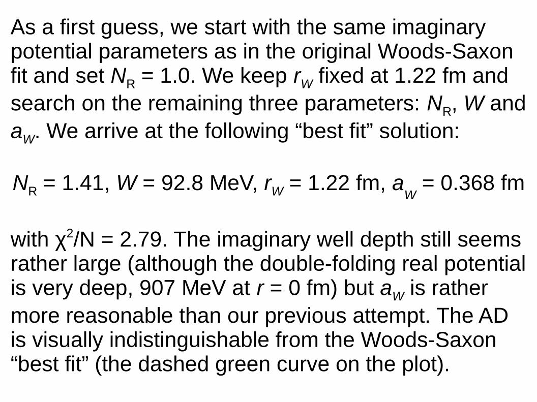
As a first guess, we start with the same imaginarypotential parameters as in the original Woods-Saxonfit and set NR = 1.0. We keep rW fixed at 1.22 fm andsearch on the remaining three parameters: NR, W andaW. We arrive at the following “best fit” solution:

NR = 1.41, W = 92.8 MeV, rW = 1.22 fm, aW = 0.368 fm

with χ2/N = 2.79. The imaginary well depth still seemsrather large (although the double-folding real potentialis very deep, 907 MeV at r = 0 fm) but aW is rather more reasonable than our previous attempt. The ADis visually indistinguishable from the Woods-Saxon“best fit” (the dashed green curve on the plot).

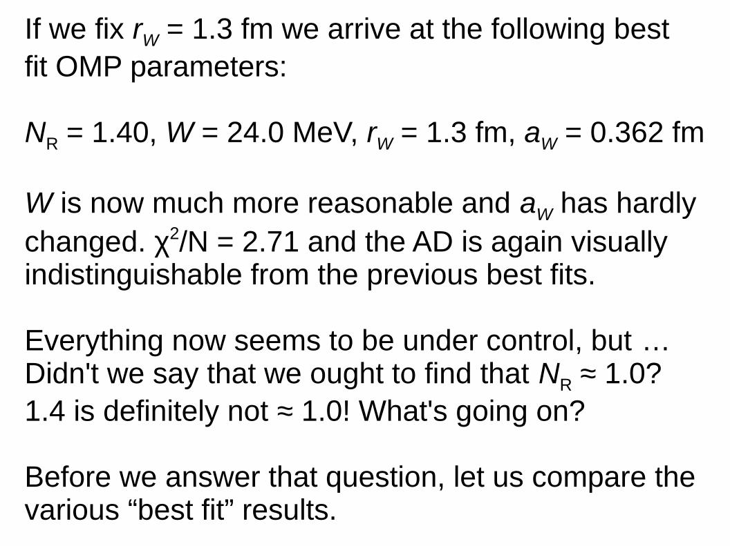
If we fix rW = 1.3 fm we arrive at the following best fit OMP parameters:

NR = 1.40, W = 24.0 MeV, rW = 1.3 fm, aW = 0.362 fm

W is now much more reasonable and aW has hardlychanged. χ2/N = 2.71 and the AD is again visuallyindistinguishable from the previous best fits.

Everything now seems to be under control, but … Didn't we say that we ought to find that NR ≈ 1.0? 1.4 is definitely not ≈ 1.0! What's going on?

Before we answer that question, let us compare the various “best fit” results.

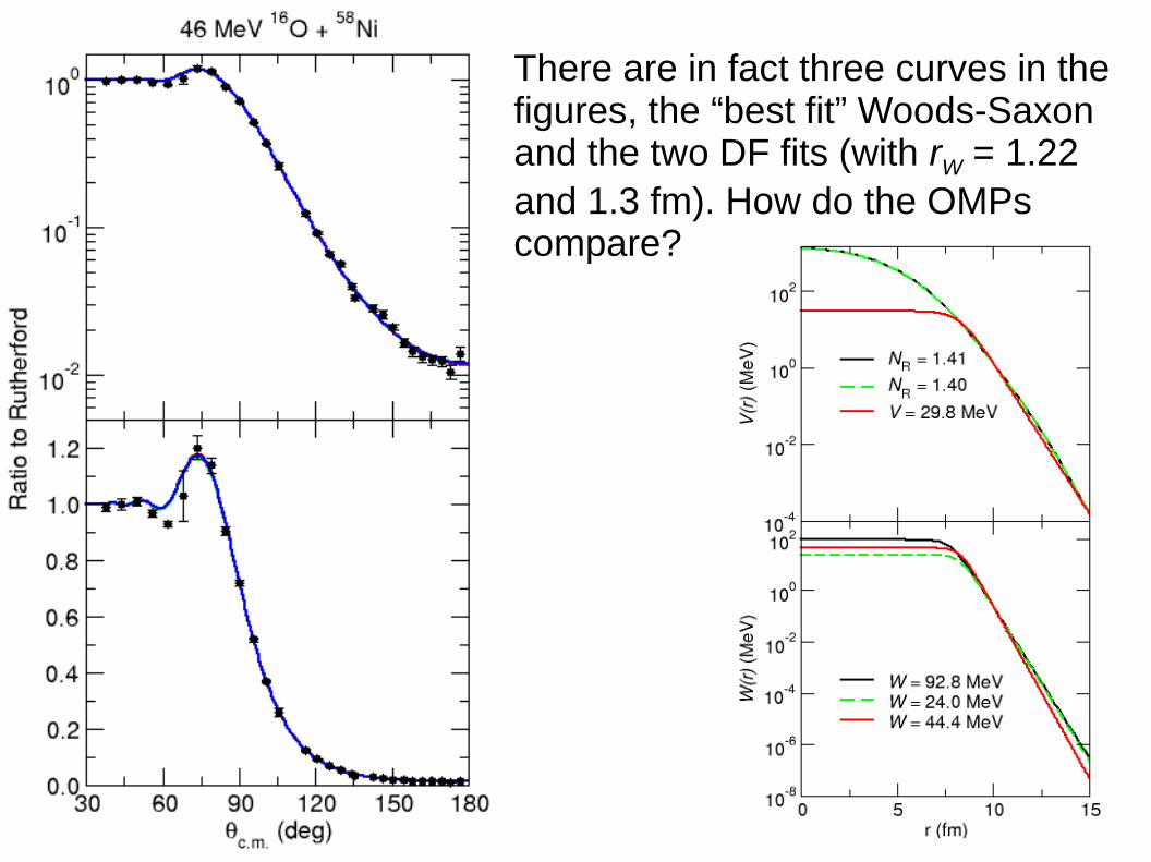
There are in fact three curves in the figures, the “best fit” Woods-Saxonand the two DF fits (with rW = 1.22and 1.3 fm). How do the OMPscompare?

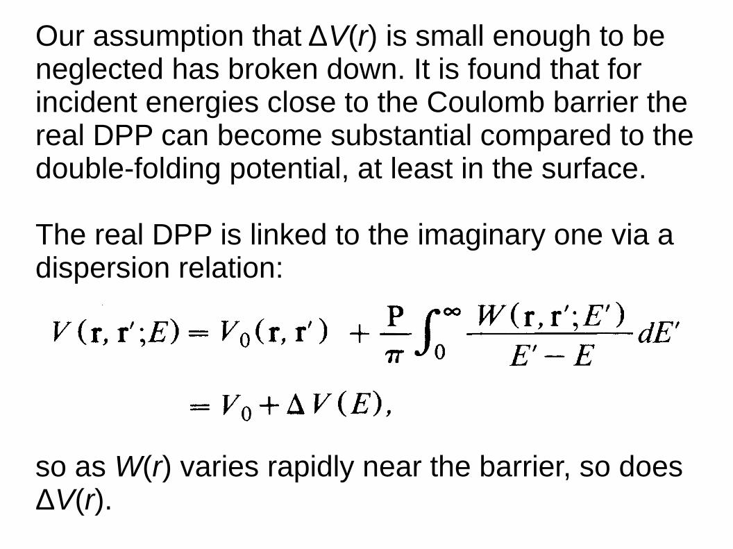
Our assumption that ΔV(r) is small enough to be neglected has broken down. It is found that for incident energies close to the Coulomb barrier the real DPP can become substantial compared to thedouble-folding potential, at least in the surface.

The real DPP is linked to the imaginary one via adispersion relation:

so as W(r) varies rapidly near the barrier, so does ΔV(r).

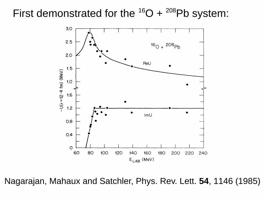
First demonstrated for the 16O + 208Pb system:

Nagarajan, Mahaux and Satchler, Phys. Rev. Lett. 54, 1146 (1985)

The effect should, in principle, be universal, but itcan be difficult to demonstrate unambiguously.

We can simulate the effect of ΔV(r) by the factor NR because for heavy ions the data are only sensitive to the potential around the surface; the effective real potential induced by couplings is peaked atthe surface.

The 16O + 58Ni system is one case where the effectis large enough to be clearly defined as an energyvariation in the surface strength of the potentials.They also follow a dispersion relation quite well …

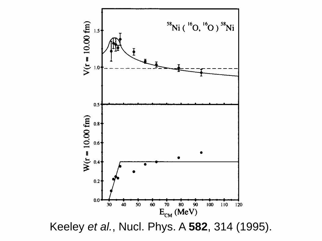
Keeley et al., Nucl. Phys. A 582, 314 (1995).

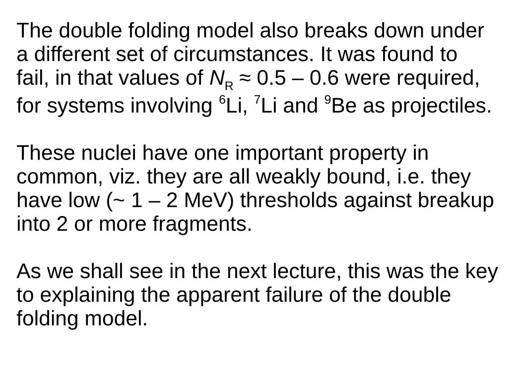
The double folding model also breaks down undera different set of circumstances. It was found tofail, in that values of NR ≈ 0.5 – 0.6 were required,for systems involving 6Li, 7Li and 9Be as projectiles.

These nuclei have one important property in common, viz. they are all weakly bound, i.e. they have low (~ 1 – 2 MeV) thresholds against breakup into 2 or more fragments.

As we shall see in the next lecture, this was the key to explaining the apparent failure of the doublefolding model.

Lecture 6: Optical model analysis of heavy ion elasticscattering continued

We saw last time that the “semi microscopic” OMPconsisting of a renormalised double folding real partand a Woods-Saxon imaginary part was able todescribe well a wide range of data with NR ≈ 1.0, withthe exception of energies close to the Coulombbarrier where ∆V(r) can be large compared to Vf(r).

Other exceptions are data for 6,7Li and 9Be projectiles:

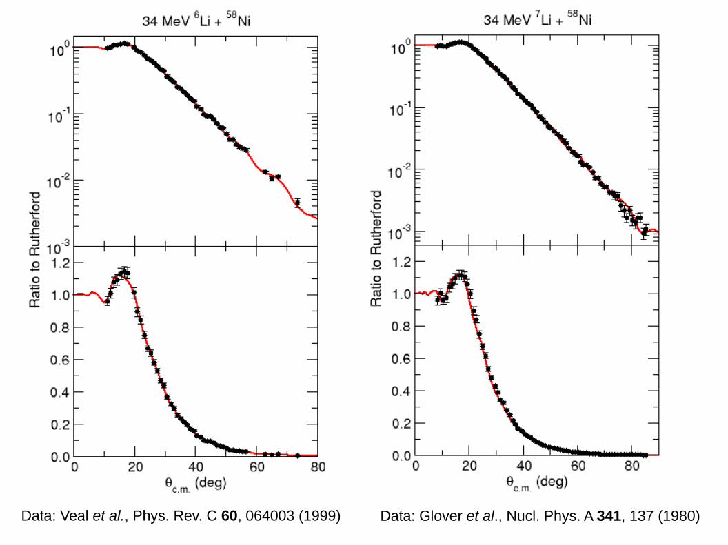
Data: Glover et al., Nucl. Phys. A 341, 137 (1980)Data: Veal et al., Phys. Rev. C 60, 064003 (1999)

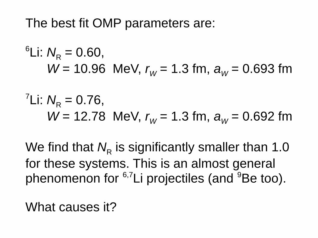
The best fit OMP parameters are:

6Li: NR = 0.60, W = 10.96 MeV, rW = 1.3 fm, aW = 0.693 fm

7Li: NR = 0.76, W = 12.78 MeV, rW = 1.3 fm, aW = 0.692 fm

We find that NR is significantly smaller than 1.0for these systems. This is an almost generalphenomenon for 6,7Li projectiles (and 9Be too).

What causes it?

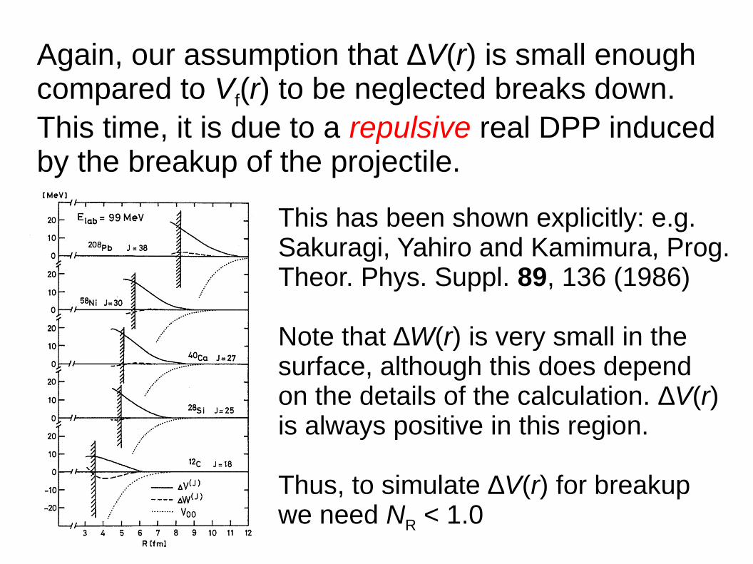
Again, our assumption that ∆V(r) is small enoughcompared to Vf(r) to be neglected breaks down.This time, it is due to a repulsive real DPP inducedby the breakup of the projectile.

This has been shown explicitly: e.g.Sakuragi, Yahiro and Kamimura, Prog. Theor. Phys. Suppl. 89, 136 (1986)

Note that ∆W(r) is very small in thesurface, although this does dependon the details of the calculation. ∆V(r)is always positive in this region.

Thus, to simulate ∆V(r) for breakupwe need NR < 1.0

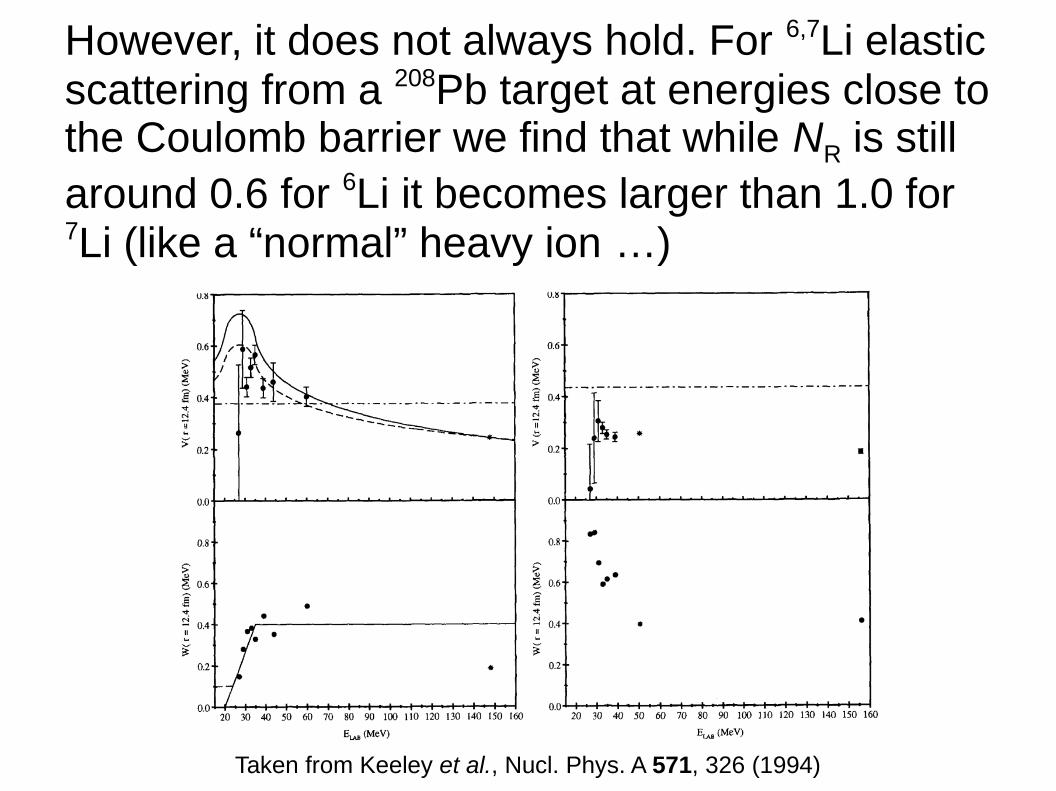
However, it does not always hold. For 6,7Li elasticscattering from a 208Pb target at energies close tothe Coulomb barrier we find that while NR is still around 0.6 for 6Li it becomes larger than 1.0 for7Li (like a “normal” heavy ion …)

Taken from Keeley et al., Nucl. Phys. A 571, 326 (1994)

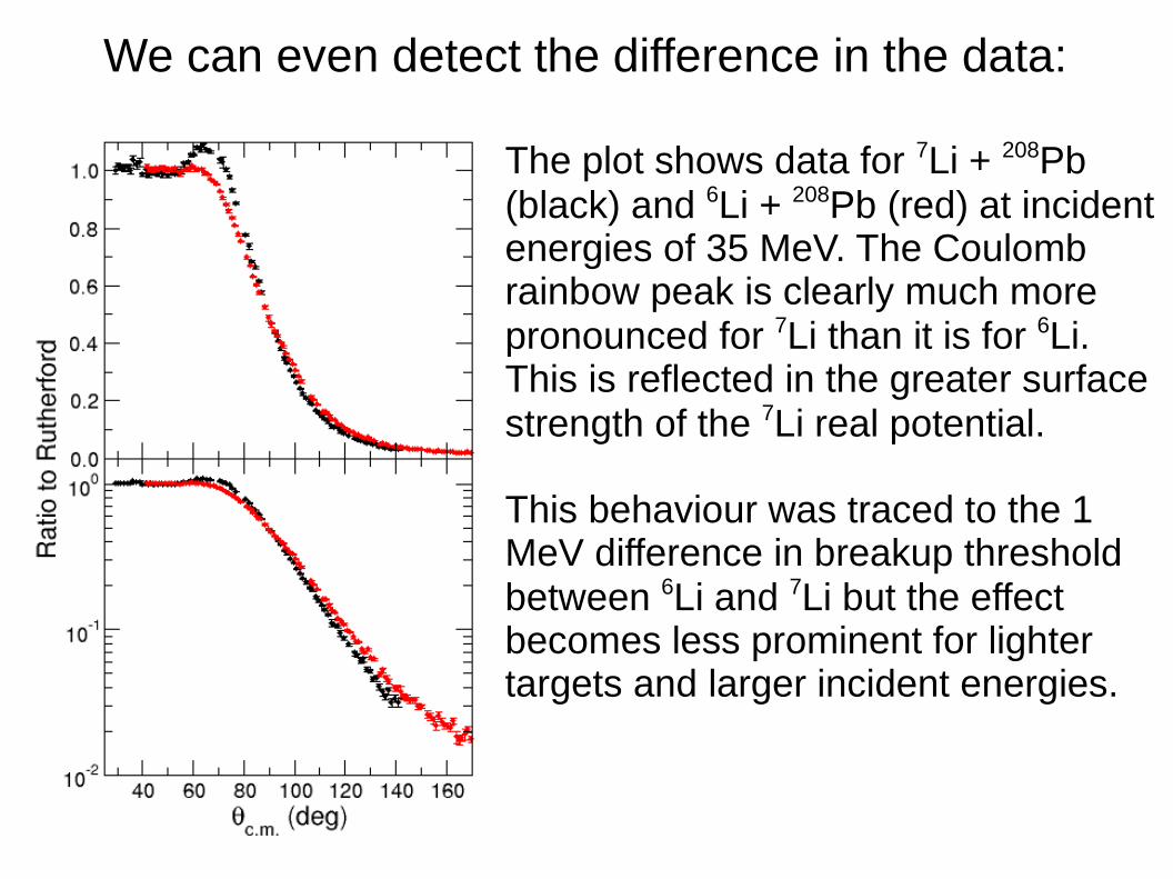
We can even detect the difference in the data:

The plot shows data for 7Li + 208Pb(black) and 6Li + 208Pb (red) at incidentenergies of 35 MeV. The Coulombrainbow peak is clearly much morepronounced for 7Li than it is for 6Li.This is reflected in the greater surfacestrength of the 7Li real potential.

This behaviour was traced to the 1MeV difference in breakup thresholdbetween 6Li and 7Li but the effectbecomes less prominent for lightertargets and larger incident energies.

This brings us quite nicely to the final part of this lecture: why study elastic scattering?

There are two answers to this question:

1) Since elastic scattering is always present, it is a vital ingredient in the analysis of other direct reactions. We need optical potentials that describe the appropriate elastic scattering as input to any analysis of inelastic scattering and transfer reactions.

2) For its own sake. Elastic scattering can provide information on the structure of the colliding nuclei itself. Coupling effects are also worthy of study.

We shall demonstrate the first point in later lectureswhen we investigate these reactions.

Here, let us return to light ion elastic scattering,specifically proton scattering.

What does proton elastic scattering actually tell us?

The rms matter radius of the target nucleus and not much else, in most cases. Using sophisticated microscopic models to calculate the proton-nucleus potentials it is found that, provided the target density used has the correct rms matter radius, the fit to the elastic scattering data is more or less insensitive to other details of the nuclear matter density.

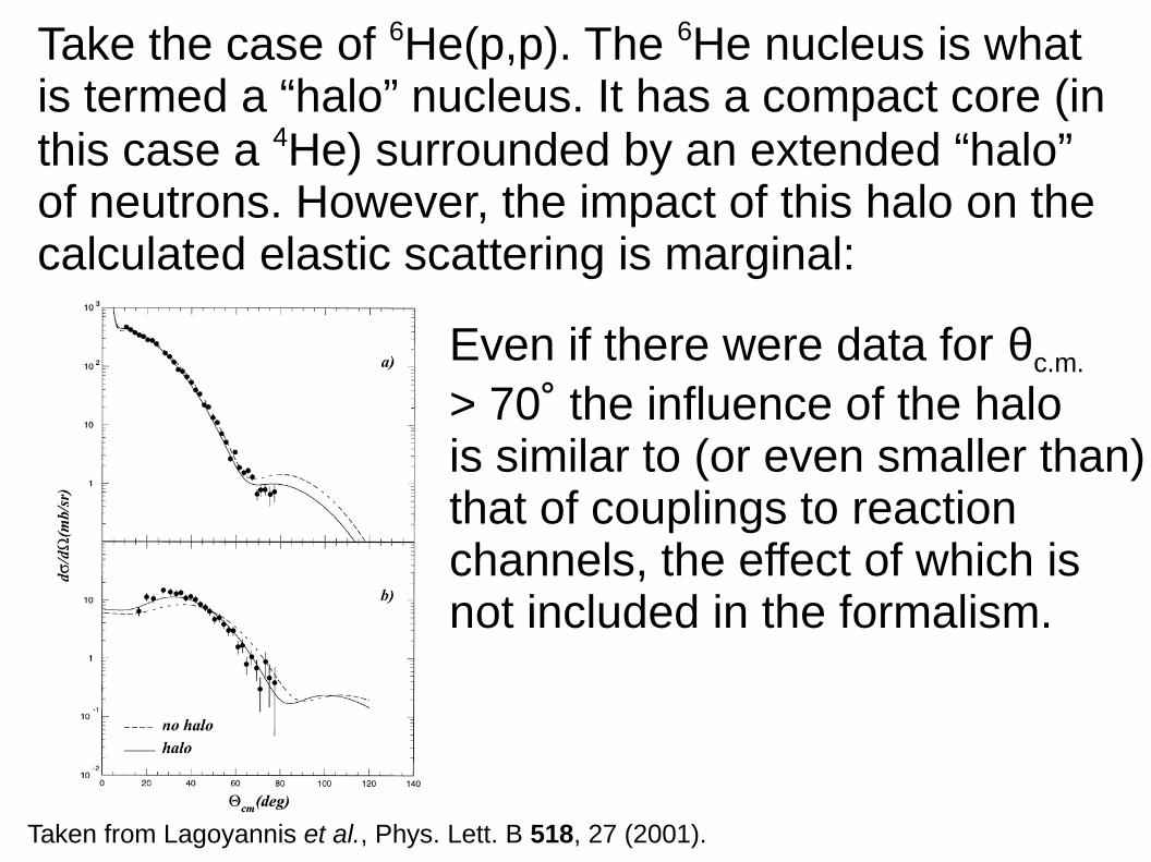
Take the case of 6He(p,p). The 6He nucleus is whatis termed a “halo” nucleus. It has a compact core (inthis case a 4He) surrounded by an extended “halo”of neutrons. However, the impact of this halo on thecalculated elastic scattering is marginal:

Taken from Lagoyannis et al., Phys. Lett. B 518, 27 (2001).

Even if there were data for θc.m.

> 70˚ the influence of the halois similar to (or even smaller than)that of couplings to reactionchannels, the effect of which isnot included in the formalism.

So much for what we might term “static” effects due to the specific nuclear structure of the target.

As we said previously though, fitting a large bodyof proton elastic scattering data with the opticalmodel may be likened to the work of Kepler inreducing Tycho Brahe's mass of planetary observations to his three laws.

It is for targets where the optical model fails (or atleast has difficulty) in fitting data with standard forms or where averaged (what we term “global”) OMP parameters describe the data poorly that we should look for “dynamic” effects due to thespecific nuclear structure.

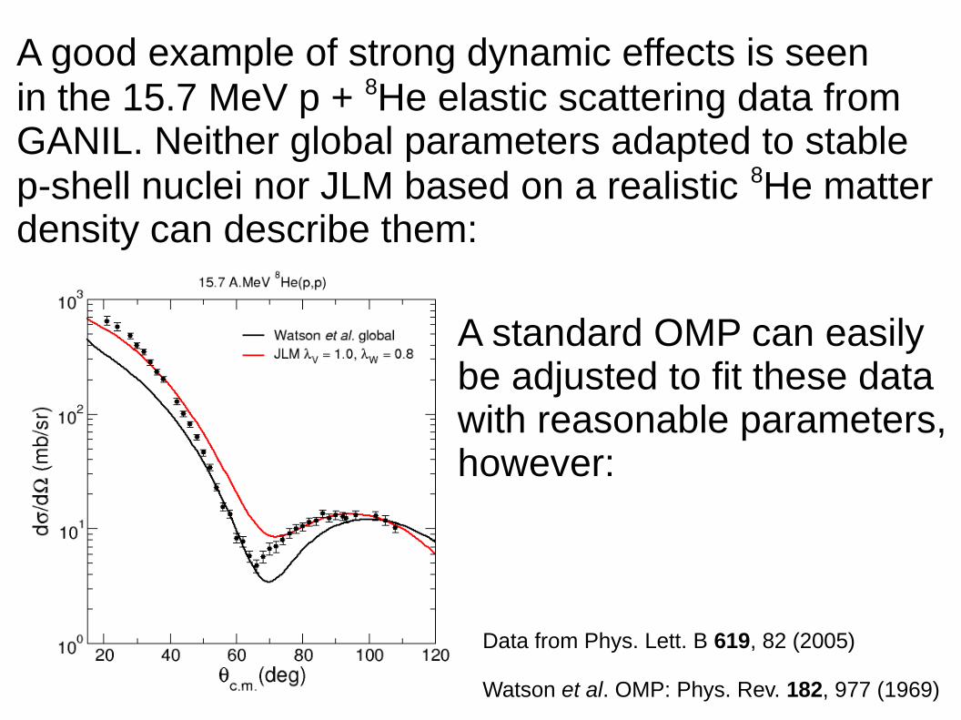
A good example of strong dynamic effects is seenin the 15.7 MeV p + 8He elastic scattering data from GANIL. Neither global parameters adapted to stable p-shell nuclei nor JLM based on a realistic 8He matter density can describe them:

A standard OMP can easilybe adjusted to fit these datawith reasonable parameters,however:

Data from Phys. Lett. B 619, 82 (2005)

Watson et al. OMP: Phys. Rev. 182, 977 (1969)

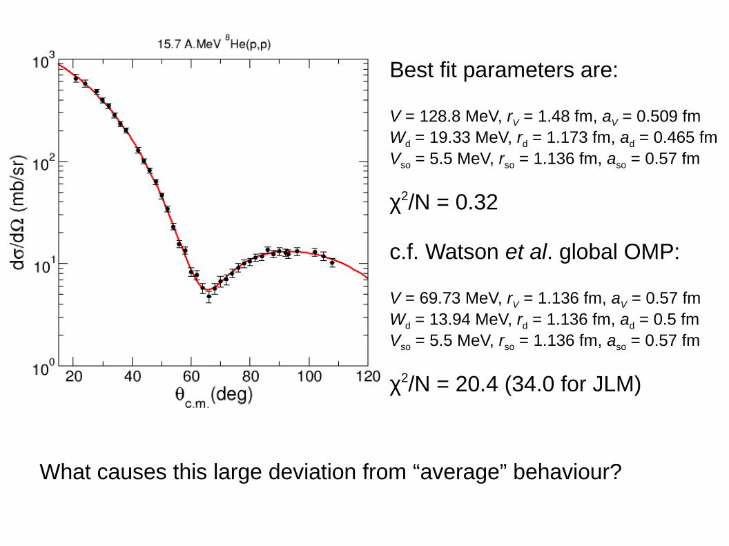
Best fit parameters are:

V = 128.8 MeV, rV = 1.48 fm, aV = 0.509 fmWd = 19.33 MeV, rd = 1.173 fm, ad = 0.465 fmVso = 5.5 MeV, rso = 1.136 fm, aso = 0.57 fm

χ2/N = 0.32

c.f. Watson et al. global OMP:

V = 69.73 MeV, rV = 1.136 fm, aV = 0.57 fmWd = 13.94 MeV, rd = 1.136 fm, ad = 0.5 fmVso = 5.5 MeV, rso = 1.136 fm, aso = 0.57 fm

χ2/N = 20.4 (34.0 for JLM)

What causes this large deviation from “average” behaviour?

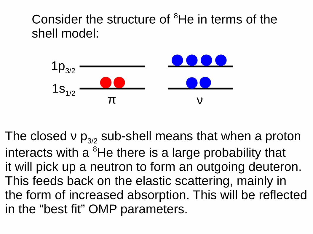
Consider the structure of 8He in terms of the shell model:

1s1/2

1p3/2

νπ

The closed ν p3/2 sub-shell means that when a protoninteracts with a 8He there is a large probability thatit will pick up a neutron to form an outgoing deuteron.This feeds back on the elastic scattering, mainly inthe form of increased absorption. This will be reflectedin the “best fit” OMP parameters.

What of heavy ion elastic scattering? Surely thatis uninteresting since it is only sensitive to theOMP in the surface? Also, it is not amenable toobtaining global potential parameters.

In fact, we have already seen that heavy ion elasticscattering can be sensitive to differences in thenuclear structure of the interacting nuclei under theright conditions:

1) Energy range – close to the Coulomb barrier2) Precise measurement – ~ 2-3 % uncertainty3) Careful choice of target and/or projectile

A sub-set of heavy ion elastic scattering data that are particularly sensitive to nuclear structure arethose systems where there is strong coupling toother reaction channels, usually inelastic excitations.

Under the right conditions such data can bequantitatively sensitive to the nuclear structure,although they are usually difficult, if not impossible,to fit with a conventional OMP.

A recent review article has dealt with this subject:Keeley, Kemper and Rusek, Eur. Phys. J. A 50, 145 (2014) so I will only show a few exampleshere.

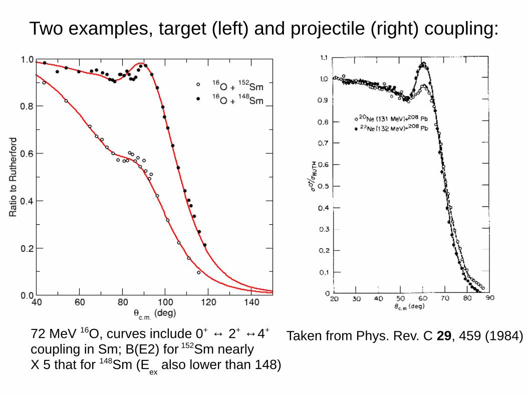
Two examples, target (left) and projectile (right) coupling:

72 MeV 16O, curves include 0+ ↔ 2+ ↔4+

coupling in Sm; B(E2) for 152Sm nearlyX 5 that for 148Sm (E

ex also lower than 148)

Taken from Phys. Rev. C 29, 459 (1984)

These are examples of strong coupling to inelastic excitations.

The elastic scattering is sensitive to the B(E2) value of therelevant coupling almost exclusively (it is the Coulombexcitation that is important here since the charge productZ1Z2 is large).

Such data are difficult to fit with an OMP of standard form.One can obtain very good descriptions either by explicitlyincluding the coupling (coupled channels calculations,as inthe previous slides, which we shall consider in the next lecture) or by adding a long-range imaginary DPP to the usual OMP.

The form of the latter can be estimated using semi-classicaltheories of Coulomb excitation and also works very well …

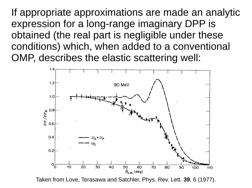
If appropriate approximations are made an analyticexpression for a long-range imaginary DPP isobtained (the real part is negligible under these conditions) which, when added to a conventional OMP, describes the elastic scattering well:

Taken from Love, Terasawa and Satchler, Phys. Rev. Lett. 39, 6 (1977).

Apart from the OMP parameters (obtained in thiscase by fitting the quasi-elastic scattering AD) theonly parameter in this model is the B(E2) value.

The only problem with this type of study is that itis essential to measure the pure elastic scattering.Since the strongly coupled states tend to have small excitation energies (~100 keV or even less)this can be a major experimental headache! Oftenmagnetic spectrometers are required to obtain thenecessary resolution, which leads to a longexperiment.

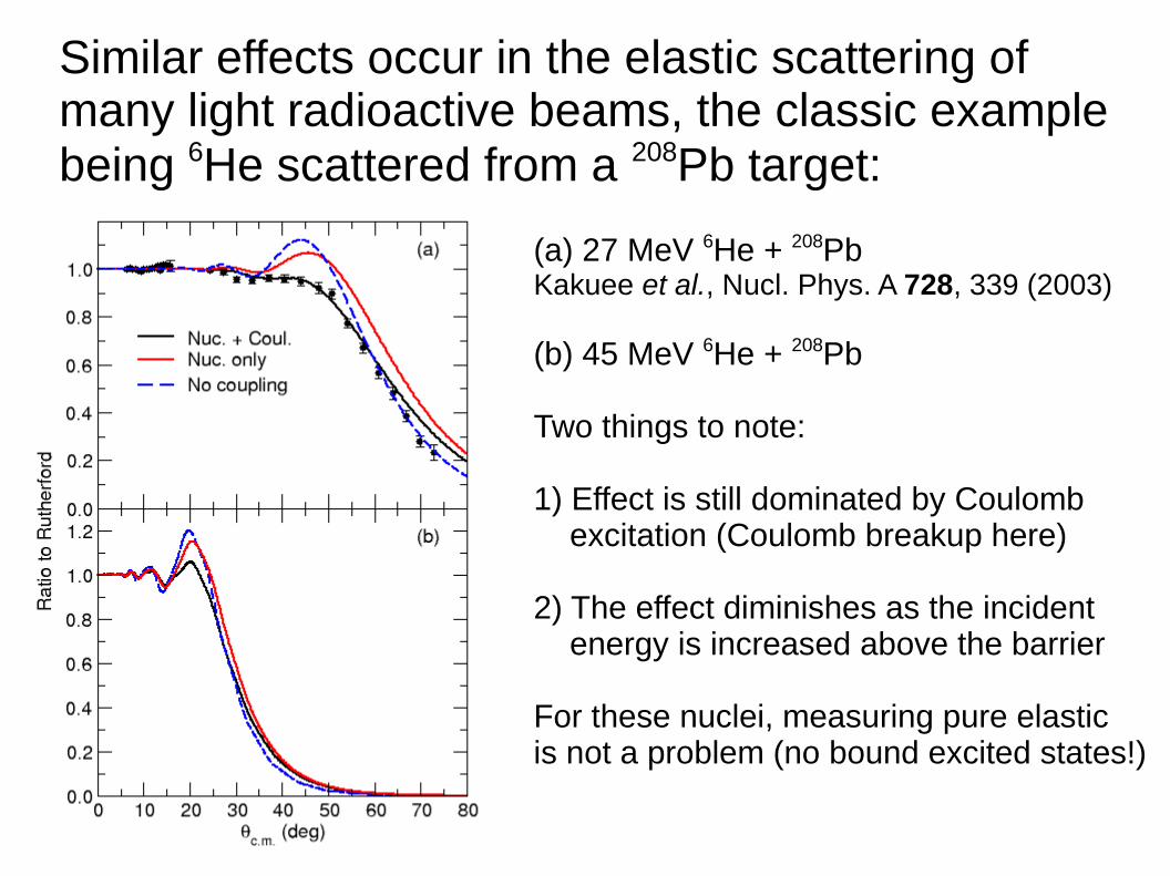
Similar effects occur in the elastic scattering ofmany light radioactive beams, the classic examplebeing 6He scattered from a 208Pb target:

(a) 27 MeV 6He + 208PbKakuee et al., Nucl. Phys. A 728, 339 (2003)

(b) 45 MeV 6He + 208Pb

Two things to note:

1) Effect is still dominated by Coulomb excitation (Coulomb breakup here)

2) The effect diminishes as the incident energy is increased above the barrier

For these nuclei, measuring pure elasticis not a problem (no bound excited states!)

There are many other examples of radioactivebeams where this behaviour is known or expected.There is still plenty of work to be done in this line.

I hope that this small digression has shown thatelastic scattering is interesting for its own sakeand not just as an ingredient to reaction studies.

Fitting data with an optical model may seem to bea somewhat pointless exercise in its own right, butsuch fits can give us clues to important physicaleffects that require more sophisticated models to describe.

Attempting to systematise large bodies of datathrough the search for simple laws that governtheir behaviour is a first step to true understanding:without Kepler's work Newton would have had amuch harder task in formulating his theory ofgravitation.

We might not yet have our Newton for elasticscattering but we certainly still need our Keplers!

Lecture 7: inelastic scattering

To recap, inelastic scattering takes place when wehave an inelastic collision between two interactingnuclei; i.e., one (or both for heavy ion projectiles)of the nuclei involved is raised to an excited state during the collision with a corresponding loss in the total kinetic energy of the system.

The excitation usually takes one of two basic forms:single particle (or hole) excitations or collectiveexcitations, subdivided into vibrational and rotationalexcitations.

This is, of course, a simplified picture, and someexcitations do not fall neatly into a particular category.

We shall not consider single particle excitations hereand concentrate on collective – vibrational androtational – excitations.

As the name implies, these are collective motions ofthe nucleus as a whole and can be pictured by analogy with the motions of a drop of liquid.

If this drop is deformed, i.e. non-spherical, in shape it can rotate about an axis of symmetry to producerotational excitations. If spherical, it can vibrate invarious ways to produce vibrational excitations.

Deformed nuclei can also vibrate, so they usuallyhave a mixture of rotational states (divided intobands of related states) and vibrational states (which may be the starting point – the band head – of a rotational band).

We will not go further into the details of nuclearstructure here – it is a specialist subject in its ownright – but will concentrate on how we model inelastic excitations using direct reaction theory.

The theory is identical for light and heavy ions,but Coulomb excitation is obviously much moreimportant for heavy ion inelastic scattering.

To begin, we take the case of an even-evenrotational nucleus. How do we model theexcitation of the first member of the ground state rotational band, i.e. the 0+ → 2+ transition?

We need to calculate the matrix elements forthe set of coupled equations (recall lecture 2).To do this we need an interaction potential thatcan take account of the collective excitations.

This is most simply done with a deformed opticalpotential. If we assume that the nucleus is permanently deformed then the radius is:

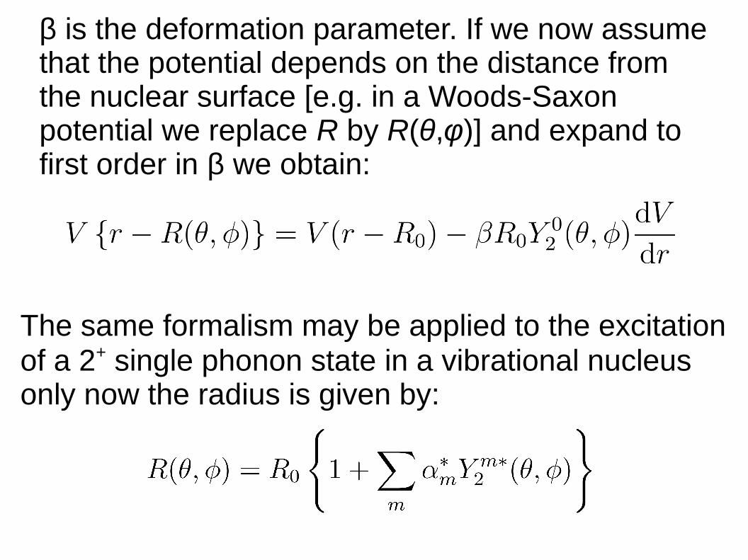
β is the deformation parameter. If we now assumethat the potential depends on the distance fromthe nuclear surface [e.g. in a Woods-Saxon potential we replace R by R(θ,φ)] and expand tofirst order in β we obtain:

The same formalism may be applied to the excitationof a 2+ single phonon state in a vibrational nucleus only now the radius is given by:

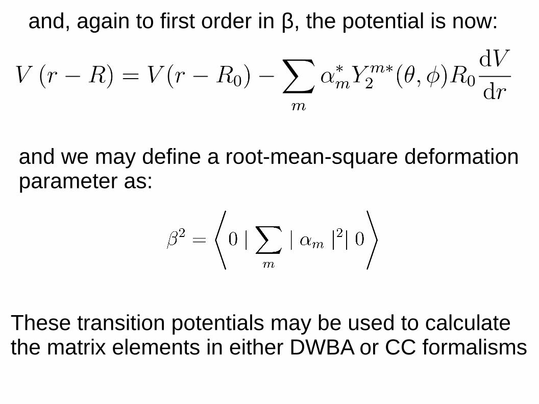
and, again to first order in β, the potential is now:

and we may define a root-mean-square deformationparameter as:

These transition potentials may be used to calculatethe matrix elements in either DWBA or CC formalisms

A similar exercise may be performed for the Coulombexcitation.

In DWBA there is no difference between excitationof a single quadrupole phonon in a vibrationalnucleus and excitation of the first 2+ state of the ground state band of a rotational nucleus.

However, if we use the more accurate CC theory,second order effects come into play, and for therotational nucleus reorientation terms appear. Theseare diagonal matrix elements linking states in differentmagnetic sub-states. They do not exist in vibrationalnuclei since these matrix elements are then zero.

In principle, CC should be used for collectivetransitions since they are strongly coupled, butDWBA is still sometimes used, particularly for thespecial case of giant resonances.

However, there are several important considerationsthat are common to both formalisms as applied toinelastic scattering.

We have seen that in addition to the spherical partof the optical potential we now need to define adeformation parameter β. In fact, this enters theequations as the combination βR0, referred to asthe deformation length, δ, usually given in fm.

Thus, in principle, we need only define β in additionto the usual optical potential to describe inelasticscattering. However, there are some choices to bemade!

1) There are nuclear and Coulomb potentials. Should βCoul = βNuc? Or should δCoul = δNuc? Or are the two independent?

2) The nuclear potential has both real and imaginary parts. Should βreal = βimag or δreal = δimag? Or are the two independent?

3) Should we deform the imaginary part at all?

To answer these questions, it should first be stressedthat both β and δ are model dependent, i.e. the exactvalue extracted by fitting a given data set will dependon the details of the model used. However, generallyδ is better defined than β and I personally prefer towork with it (most reaction codes use β, althoughFRESCO uses δ).

In principle, one expects that the Coulomb and nuclear responses should be the same in the collective model, so we would expect δCoul = δNuc. However, remember that our “nuclear fluid” hastwo components, neutrons and protons …

The Coulomb response depends on the distribution of the protons alone, whereas the nuclear responsewill also depend on the distribution of the neutrons. They need not coincide exactly, and for more exotic nuclei there is no a priori reason why δCoul = δNuc.

However, the nuclear response ought to be the samefor both real and imaginary parts. Since R0 will notin general be the same for both parts I prefer to fixδreal = δimag. It is, however, a moot point whether oneshould deform the imaginary part of the potential atall; certainly for heavy ions fits to data are worse ifthis is not done.

We can at least avoid the question of what to takefor βCoul (or δCoul) by using the B(Eλ) value insteadfor the Coulomb coupling.

B(Eλ) is the electric transition probability for the2λ-pole transition and is usually expressed in units of e2bλ, where e is the charge on the electron. N.B.in reaction work we use B(Eλ)↑, unlike in gammaspectroscopy where B(Eλ)↓ is quoted.

FRESCO, for example, uses the reduced matrixelements for Coulomb excitation, related to theB(Eλ). Other codes use βλ for the Coulomb as wellas the nuclear excitation.

The advantage of using B(Eλ) is that it can beindependently determined (e.g. by electron scatteringor Coulomb excitation) and is thus independent ofthe charge radius chosen. We can relate B(Eλ) toβ

λ within the collective model as follows:

B(Eλ) = (3/4π)2 (ZeRλ)2βλ2

where R is the nuclear charge radius. Thus, thevalue of β

λ obtained depends on the choice of R.

How does all this work out in practice? Let us take afew typical examples of inelastic excitation with bothlight and heavy ions.

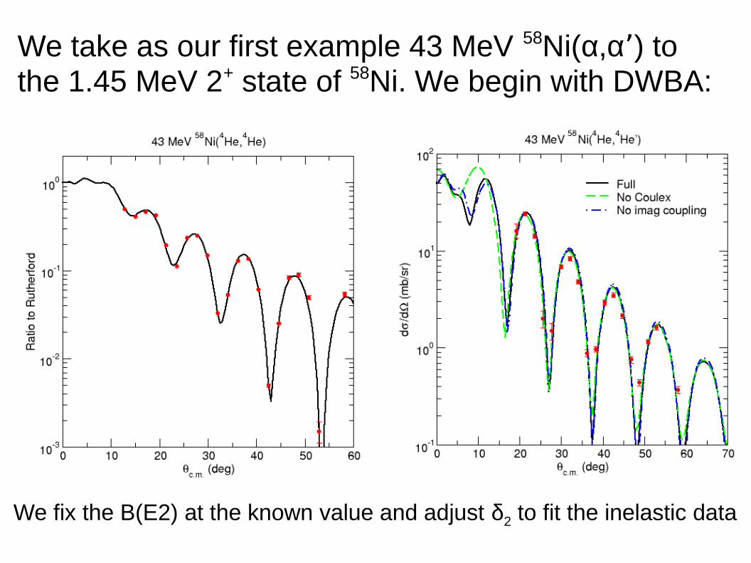
We take as our first example 43 MeV 58Ni(α,α ) toʼthe 1.45 MeV 2+ state of 58Ni. We begin with DWBA:

We fix the B(E2) at the known value and adjust δ2 to fit the inelastic data

The description is good, we obtain δ2 = 1.10 fm.

Note that we are insensitive to the inclusion of animaginary coupling potential in this case, and onlysensitive to the inclusion of Coulomb excitation atforward angles (where there are no data).

Thus, for inelastic scattering of α particles from amedium mass vibrational target nucleus DWBAseems to work well. What do we find if we performa coupled channels analysis?

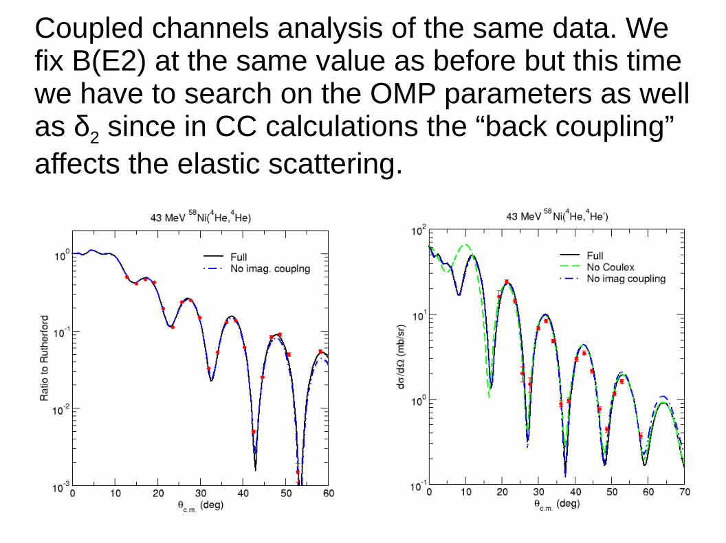
Coupled channels analysis of the same data. Wefix B(E2) at the same value as before but this timewe have to search on the OMP parameters as wellas δ2 since in CC calculations the “back coupling”affects the elastic scattering.

The result is very similar to DWBA, although wehave had to readjust the OMP parameters. Weagain see little sensitivity to the inclusion of eitherCoulomb excitation or imaginary coupling potentials(the omission of the latter does have a slight effecton the elastic scattering).

The value of δ2 obtained is 10 % smaller than in DWBA, δ2 = 1.00 fm, within the likely uncertainty.

Thus in this case DWBA seems perfectly adequate.This is largely due to the relatively weak couplingstrength.

As an example of a vibrational coupling in heavyion inelastic scattering, we stick with a 58Ni targetbut this time excite it with a 16O beam. We againperform both DWBA and CC analyses and assessthe importance of Coulomb excitation and theimaginary coupling.

We take as our data set elastic and inelastic scattering (to the 58Ni 1.45 MeV 2+ state) at 16Oincident energy of 42 MeV. We again include justthe 0+ → 2+ coupling in the 58Ni target, as in theα scattering, fixing the B(E2) at the same value.

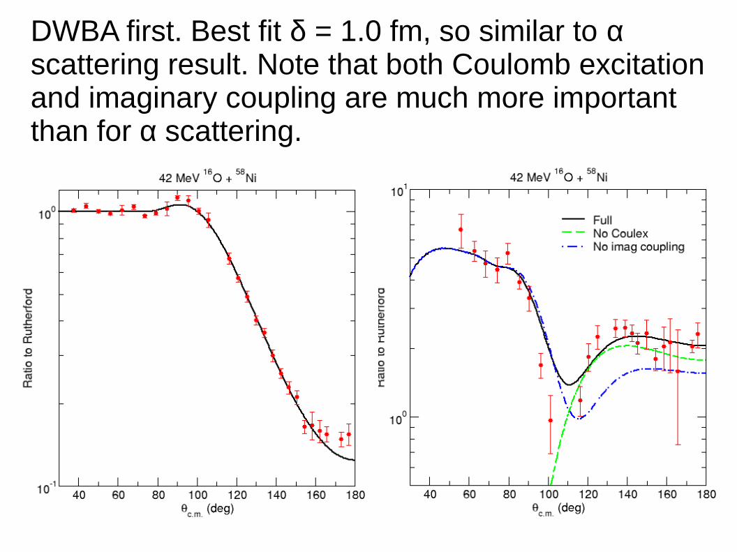
DWBA first. Best fit δ = 1.0 fm, so similar to αscattering result. Note that both Coulomb excitationand imaginary coupling are much more importantthan for α scattering.

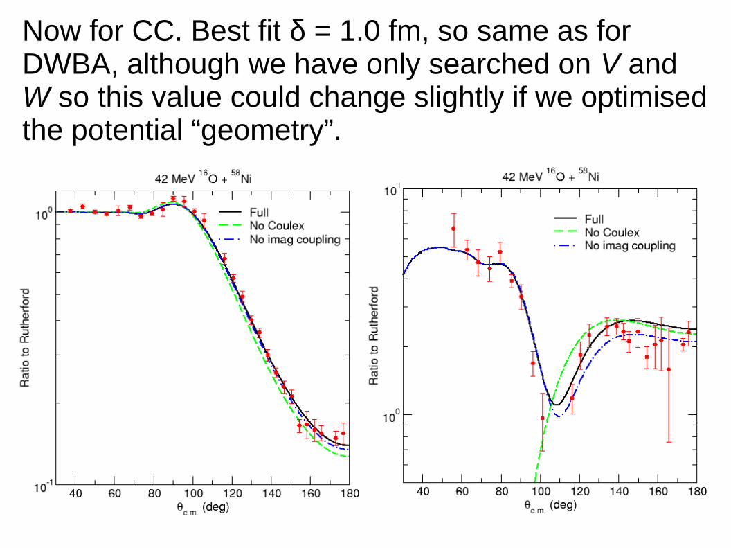
Now for CC. Best fit δ = 1.0 fm, so same as forDWBA, although we have only searched on V andW so this value could change slightly if we optimisedthe potential “geometry”.

Thus, for heavy ions we also find that DWBA isadequate for a typical vibrational nucleus, although CC does give more consistent results for data sets at different incident energies.

Coulomb excitation is important (as expected) butwe also find that imaginary couplings have asignificant influence on the inelastic scattering,although this is smaller for CC than for DWBA.

How well does the simple collective model accountfor couplings to a rotational band?

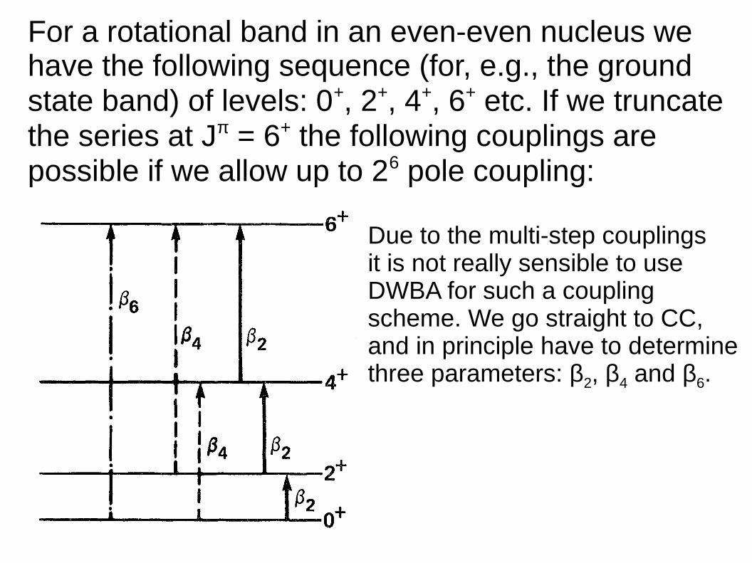
For a rotational band in an even-even nucleus wehave the following sequence (for, e.g., the groundstate band) of levels: 0+, 2+, 4+, 6+ etc. If we truncatethe series at Jπ = 6+ the following couplings arepossible if we allow up to 26 pole coupling:

Due to the multi-step couplingsit is not really sensible to useDWBA for such a coupling scheme. We go straight to CC, and in principle have to determinethree parameters: β2, β4 and β6.

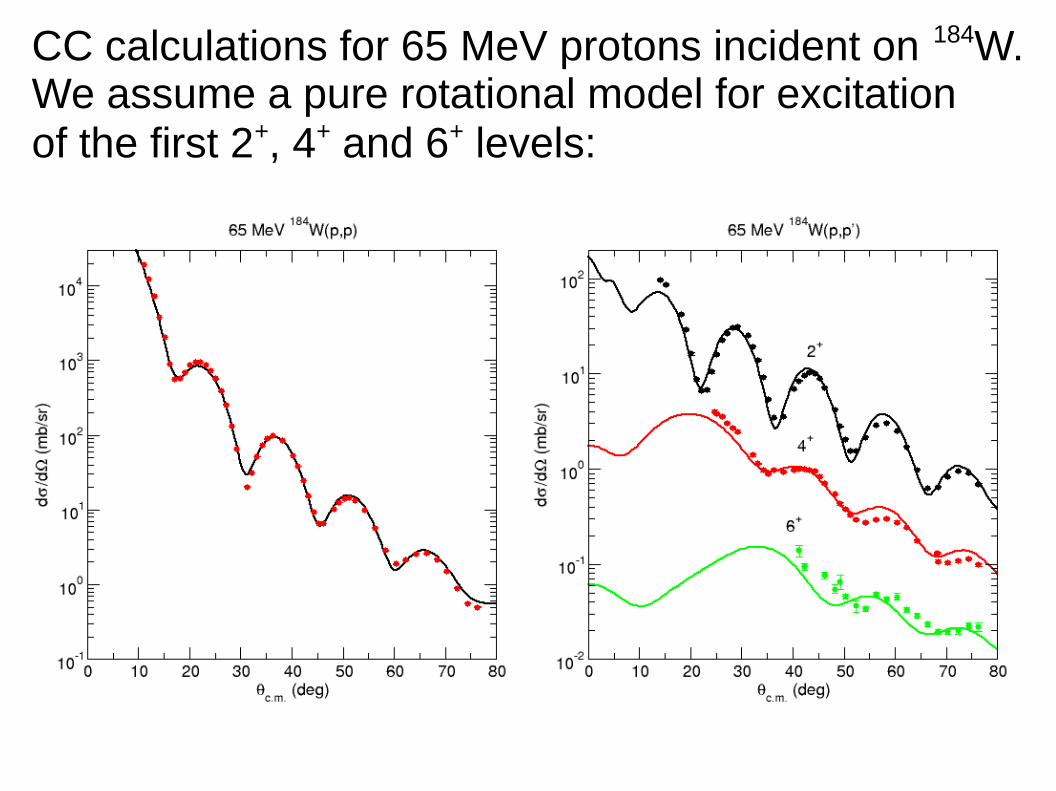
CC calculations for 65 MeV protons incident on 184W.We assume a pure rotational model for excitationof the first 2+, 4+ and 6+ levels:

Agreement is reasonable. Calculations do notinclude 26 pole couplings: evidence for thesein this case is marginal (at least with the available data). At least we can say that any26 pole coupling strength is small in this model.

We have thus seen that the pure rotational modelalso works rather well in a CC calculation.

In the next lecture we look at some refinementsin how the calculations are performed andinvestigate semi-microscopic methods.

Lecture 8: inelastic scattering continued

In the previous lecture we saw how DWBA or CCcalculations using the collective model were ableto describe rather well data for systems with collectivemotion.

However, you will recall that we simplified the treatment by only taking the expansion of thedeformed radius to first order in β. This has been standard practice for many years, but is known to be a relatively poor approximation if β is large.

Since DWBA is first order anyway refinements onlymake sense for CC calculations.

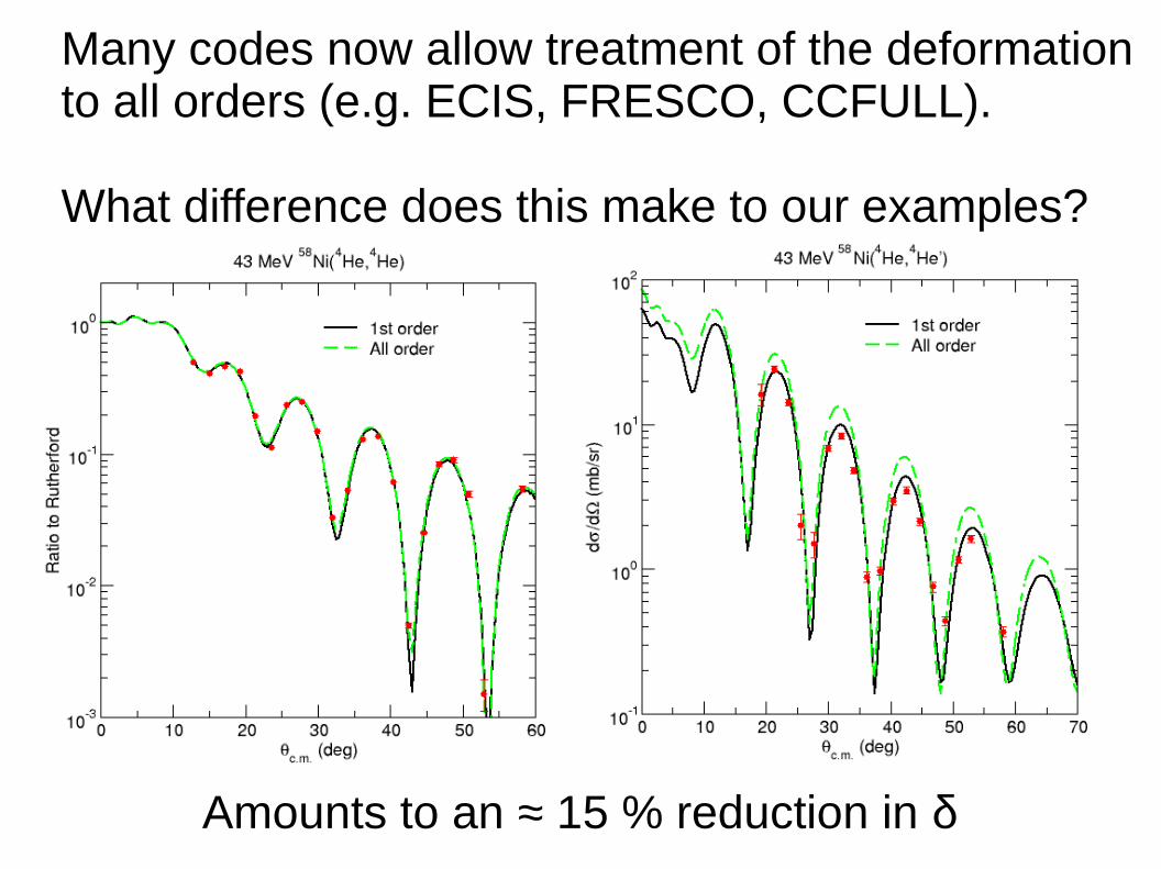
Many codes now allow treatment of the deformationto all orders (e.g. ECIS, FRESCO, CCFULL).

What difference does this make to our examples?

Amounts to an ≈ 15 % reduction in δ

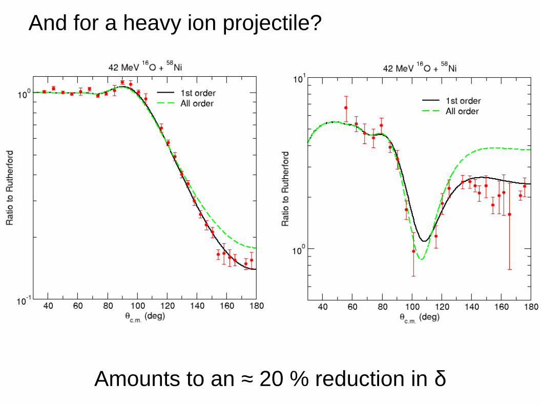
And for a heavy ion projectile?

Amounts to an ≈ 20 % reduction in δ

We find that even for a relatively weak vibrationalcoupling (the 0+ → 2+ coupling in 58Ni) there is asignificant change in the value of the deformationextracted if we go to all order, even if the shapesof the angular distributions are not significantlyaltered.

What happens in our rotational coupling casewhere the coupling strengths are stronger?

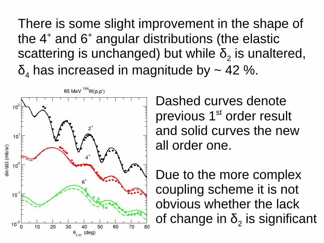
There is some slight improvement in the shape ofthe 4+ and 6+ angular distributions (the elasticscattering is unchanged) but while δ2 is unaltered,δ4 has increased in magnitude by ~ 42 %.

Dashed curves denoteprevious 1st order resultand solid curves the newall order one.

Due to the more complexcoupling scheme it is notobvious whether the lack of change in δ2 is significant

Since the question of all order versus first orderonly affects the nuclear excitation (it does not applyto the Coulomb excitation part) it will be seen thatdrawing quantitative conclusions from deformationparameters (either β or δ) extracted from fits toinelastic scattering data can be problematic.

This is particularly so if we want to look for evidenceof βCoul ≠ βNuc.

We have also confined ourselves to the strict collective model (at least for the rotational case)in that within a given band βλ values (includingreorientation couplings) are the same for alltransitions.

This need not be the case, and in general it is nottrue (although it is often a good approximation). Ifthe information is available (e.g. static quadrupolemoments of non spin-zero states for reorientationcouplings) most codes allow the strength of eachcoupling to be set individually.

One could of course try to determine the individualstrengths by fitting a set of inelastic scatteringdata. This brings us back to the old problem of trying to fit more parameters to a limited data set, but there can be cases where it is impossible adequately to “fit the elephant” otherwise!

Ultimately, how serious this model dependence of the nuclear deformation parameters is willdepend on the use one wishes to make of theinelastic scattering data. If one is attempting todraw nuclear structure conclusions from β or δvalues extracted from inelastic scattering datait can be a significant problem.

On the contrary, if one is mainly interested in thecoupling effect of inelastic excitations on theelastic scattering (often the case in heavy ion work)then it is only a problem if one is constrained to take β or δ from analyses in the literature, whencare should be taken to use the same model.

It would, of course, be more satisfying if we couldin some way calculate the transition strengthsusing a nuclear structure model (which might in principle be more sophisticated than the simple collective model).

Obviously, in the light of what we have just said, calculating the deformation parameters alone wouldnot help us much. Is there another way?

Yes: we may go back to the folding models we discussed for elastic scattering (JLM for nucleonsor double-folding for heavy ions). We can equallywell use these models with a transition densityreplacing one of the ground state matter densities.

These transition densities may be calculated usinga structure model (just as the ground state densitiescould) and used to calculate the transition potentialsrequired in our inelastic excitation calculations.

Alternatively, we may take a semi-empirical approachand deform the appropriate ground state density (asopposed to the OMP). This is known as the Tassiemodel.

Both approaches also get round a problem that may have occurred to you: all* the transition potentials in the “standard” collective model have the same radial shape. There is no reason why this should be so in reality.* Almost all. Monopole and dipole transitions have a different form

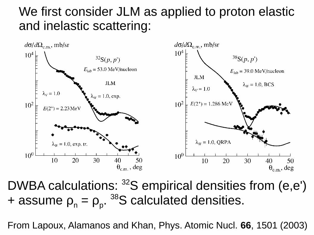
We first consider JLM as applied to proton elasticand inelastic scattering:

DWBA calculations: 32S empirical densities from (e,e')+ assume ρn = ρp.

38S calculated densities.

From Lapoux, Alamanos and Khan, Phys. Atomic Nucl. 66, 1501 (2003)

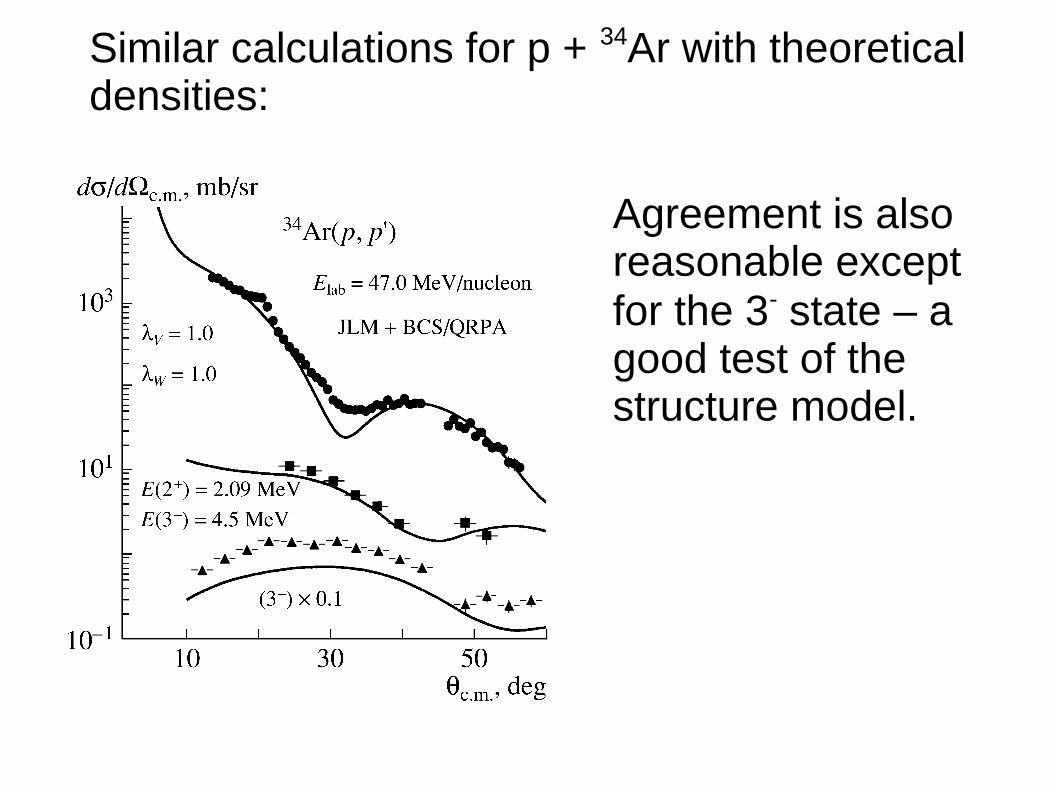
Similar calculations for p + 34Ar with theoreticaldensities:

Agreement is alsoreasonable exceptfor the 3- state – agood test of thestructure model.

JLM has the advantage that it calculates a complex OMP, so the imaginary excitation can be calculated in exactly the same way as the real.

In heavy ion work, if we use the double folding model to calculate the transition potentials as well as the diagonal OMP we are still left with the problem of what to do about the imaginary coupling potentials, since the M3Y and similar effective interactions are purely real.

One could use the DF potential for both, but there is no real physical justification for this and it places a heavy constraint on our OMP.

We therefore usually adopt a compromise: use the double folding method to calculate the real potentials (both scattering and transition) with either calculated or empirical densities (and possibly the Tassie model for the transition densities) and stick to the standard prescription for the imaginary part.

This complicates things a little if we wish to keep thereal and imaginary deformations identical (either β orδ).

Alternatively we may ignore imaginary couplings andhope to include all important couplings explicitly.

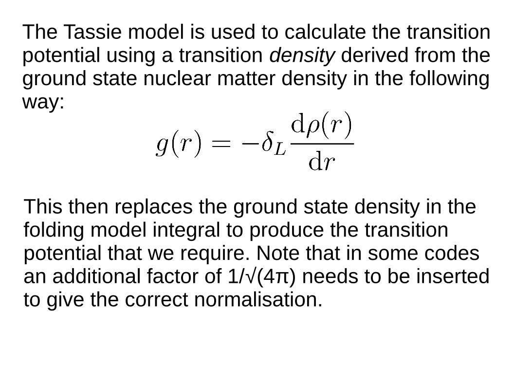
The Tassie model is used to calculate the transitionpotential using a transition density derived from theground state nuclear matter density in the followingway:

This then replaces the ground state density in the folding model integral to produce the transitionpotential that we require. Note that in some codesan additional factor of 1/√(4π) needs to be insertedto give the correct normalisation.

How does the Tassie model compare to the “standard”deformed potential model in an actual application?

Let us return to our example of 42 MeV 58Ni(16O,16O')We calculate the real transition potential in two ways:

1) Using the Tassie model by deforming the 58Ni ground state density

2) In the “standard” fashion by deforming the double folded real potential

In each case we use the same δ value and imaginarycoupling potential (diagonal potentials are also thesame in both cases).

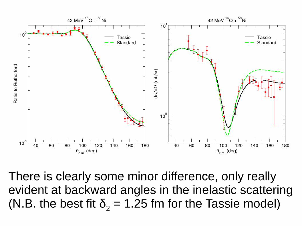
There is clearly some minor difference, only reallyevident at backward angles in the inelastic scattering(N.B. the best fit δ2 = 1.25 fm for the Tassie model)

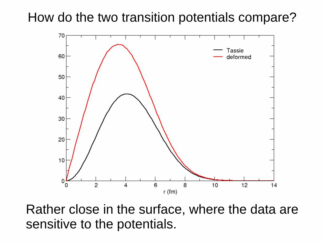
How do the two transition potentials compare?

Rather close in the surface, where the data aresensitive to the potentials.

We see that using the double folding model tocalculate transition potentials does make somedifference – the δ values are usually somewhat larger than with the usual deformed potential model.

However, if the Tassie model is used to obtain thetransition densities it is only first order in δ, so mightnot be as accurate as we could wish for strongcouplings.

Again, there are choices to be made and the valueswe extract for deformation parameters are modeldependent.

To summarise, why do we study inelastic scattering?

Inelastic scattering of the type we have beendiscussing here preferentially excites the strongcollective excitations of nuclei, thus making it agood probe of such excitations.

The “standard” approach using a deformed potentialmodel is problematic if we wish to draw detailedstructure conclusions – not only are the deformationparameters obtained model dependent but therelation of the potential deformations to those of thedensity distribution is not obvious.

Nevertheless, inelastic scattering, particularly ofprotons, is a valuable tool for probing the nuclearresponse of nuclei.

For proton scattering, JLM or similar models maybe used in conjunction with theoretical densities(both diagonal and transition) to calculate theinelastic scattering. In this way we can have a moredirect comparison between structure theory anddirect reaction data.

Such analyses can provide evidence for neutronhalo effects and the breakdown of old and theappearance of new magic numbers.

Lecture 9: transfer reactions

Transfer, or rearrangement, reactions are perhaps the most important type of direct reaction in nuclearphysics. Beyond their intrinsic interest they are a valuable tool for the extraction of nuclear structureinformation.

Their value for structure studies arises mostly dueto their selectivity: reactions such as (d,p) and (p,d)preferentially populate single particle and singlehole states respectively.

In the right energy regime direct reactions also havea very useful characteristic …

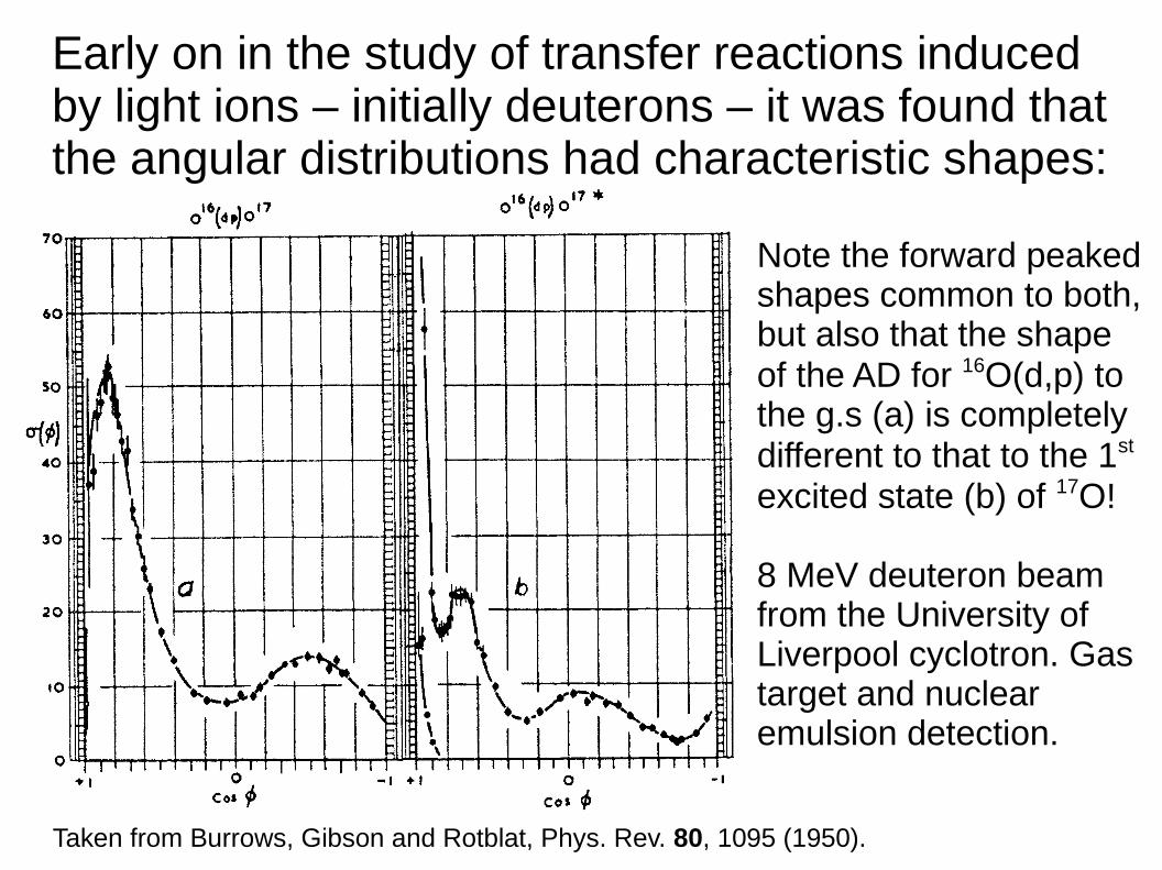
Early on in the study of transfer reactions inducedby light ions – initially deuterons – it was found thatthe angular distributions had characteristic shapes:

Note the forward peakedshapes common to both,but also that the shape of the AD for 16O(d,p) to the g.s (a) is completelydifferent to that to the 1st excited state (b) of 17O!

8 MeV deuteron beamfrom the University ofLiverpool cyclotron. Gastarget and nuclearemulsion detection.

Taken from Burrows, Gibson and Rotblat, Phys. Rev. 80, 1095 (1950).

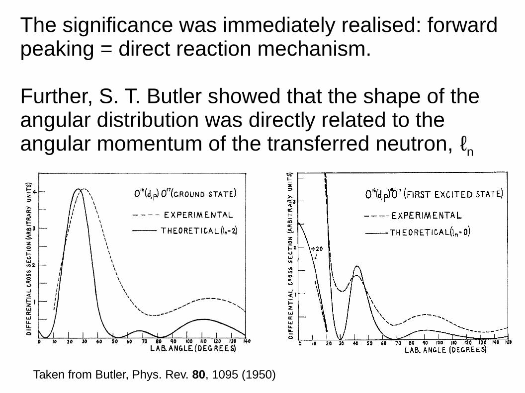
The significance was immediately realised: forward peaking = direct reaction mechanism.

Further, S. T. Butler showed that the shape of theangular distribution was directly related to theangular momentum of the transferred neutron, ℓn

Taken from Butler, Phys. Rev. 80, 1095 (1950)

This had enormous consequences for the subsequent development of direct reaction studies.

As Burrows et al. put it in their original note: “… it appears that (d, n) and (d, p) angular distributions may be of use in determining the spins and parities of ground and excited states in many nuclei.”

It was quickly realised that Butler's theory was infact equivalent to the plane wave Born approximation.This naturally prompted interest in examining the useof the distorted wave Born approximation (DWBA),first formulated in this context by Tobocman in 1958.

A significant problem with Butler theory was that not only were the shapes of the angular distributions only reproduced in general outline, but the magnitudes of the calculated cross sections bore no relation to the measured ones.

DWBA solved both problems. We may write the expression for the transfer angular distribution as :

dσ(θ,E)/dΩ = SJLFJL(θ,E)

where FJL(θ,E) is a factor containing all the reactioninformation (dependence on angle and energy) whileSJL contains structure information – the spectroscopicfactor

We may calculate FJL with an appropriate theory.The spectroscopic factor is then determined bynormalising the calculated to the measured angular distribution. With Butler theory the SJL

obtained made little or no sense.

It is important to note that SJL is not an observable,either in the quantum mechanical sense or in thesense that it can be measured. It is a derivedquantity and therefore model dependent, a factthat should always be borne in mind. The phrase“experimental spectroscopic factor” is in factnonsense in the literal sense.

In this lecture we shall examine how FJL is calculatedusing DWBA.

This will involve us in presenting a few equationsagain, but only to illustrate some of the quantitieswe need to calculate.

To begin with, DWBA comes in two “flavours”: zerorange and finite range. Each “flavour” can beformulated in one of two ways, known as post andprior. Which one we choose will depend on the typeof reaction we wish to model.

What do these expressions actually mean in termsof the formulation of DWBA?

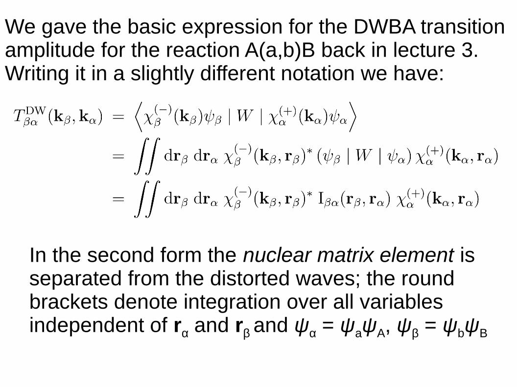
We gave the basic expression for the DWBA transition amplitude for the reaction A(a,b)B back in lecture 3.Writing it in a slightly different notation we have:

In the second form the nuclear matrix element isseparated from the distorted waves; the roundbrackets denote integration over all variables independent of rα and rβ and ψα = ψaψA, ψβ = ψbψB

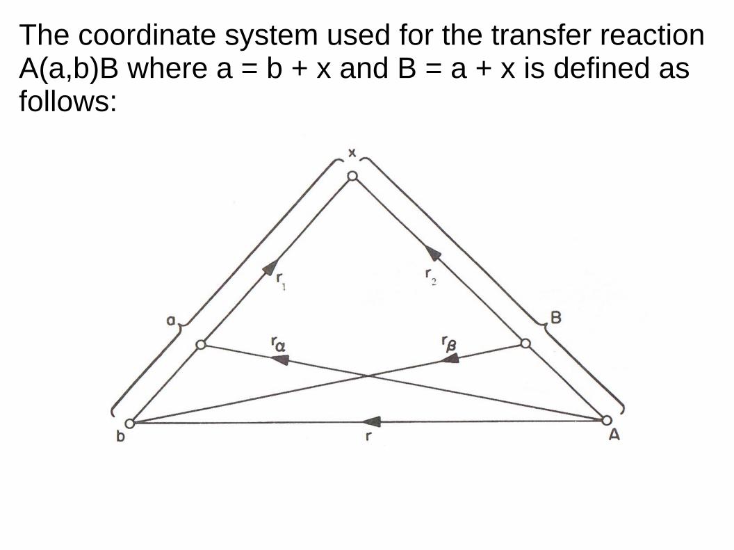
The coordinate system used for the transfer reaction A(a,b)B where a = b + x and B = a + x is defined asfollows:

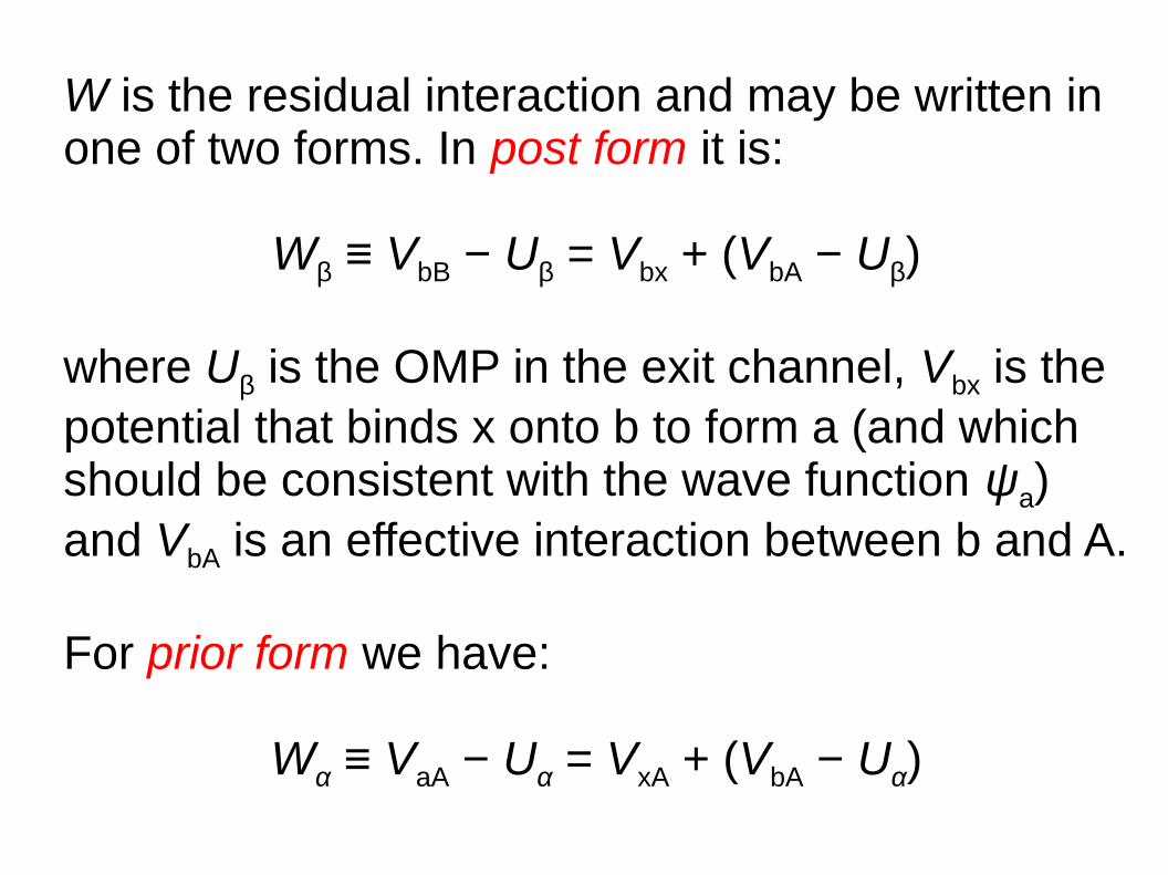
W is the residual interaction and may be written inone of two forms. In post form it is:

Wβ ≡ VbB − Uβ = Vbx + (VbA − Uβ)

where Uβ is the OMP in the exit channel, Vbx is the potential that binds x onto b to form a (and whichshould be consistent with the wave function ψa)and VbA is an effective interaction between b and A.

For prior form we have:

Wα ≡ VaA − Uα = VxA + (VbA − Uα)

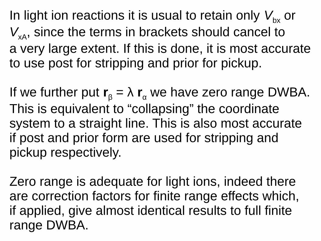
In light ion reactions it is usual to retain only Vbx orVxA, since the terms in brackets should cancel toa very large extent. If this is done, it is most accurateto use post for stripping and prior for pickup.

If we further put rβ = λ rα we have zero range DWBA.This is equivalent to “collapsing” the coordinatesystem to a straight line. This is also most accurateif post and prior form are used for stripping andpickup respectively.

Zero range is adequate for light ions, indeed there are correction factors for finite range effects which,if applied, give almost identical results to full finiterange DWBA.

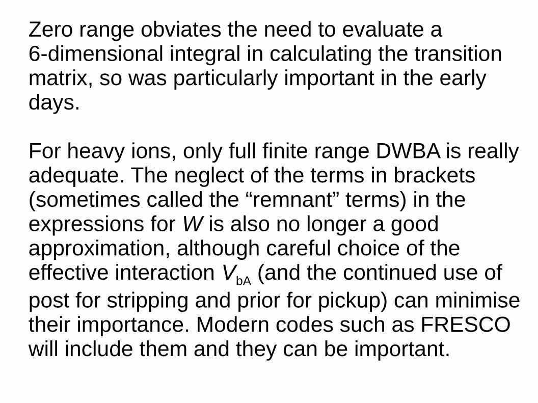
Zero range obviates the need to evaluate a 6-dimensional integral in calculating the transition matrix, so was particularly important in the earlydays.

For heavy ions, only full finite range DWBA is reallyadequate. The neglect of the terms in brackets(sometimes called the “remnant” terms) in the expressions for W is also no longer a goodapproximation, although careful choice of the effective interaction VbA (and the continued use ofpost for stripping and prior for pickup) can minimisetheir importance. Modern codes such as FRESCOwill include them and they can be important.

Finally, we come to how a DWBA calculation isperformed in practice. What are the “ingredients”that we need to assemble?

1) We need the distorted waves in the entrance and exit channels. These are calculated for us by the DWBA code from the appropriate OMPs

2) The residual interaction W. This usually boils down simply to the choice of the binding potential Vbx (post) or VxA (prior)

3) The nuclear wave function overlaps (ψB,ψA) and (ψa,ψb)

There is some overlap between 2) and 3) in actualapplications, since the wave functions required in3) are usually calculated by the code with bindingpotentials that should be consistent with the Vbx

or VxA of 2) depending on the choice of post orprior form.

Further, for 3) we also need to define 3 quantumnumbers: N ℓ j. To illustrate what these mean in the most simple way we will take a specific example, the 12C(d,p)13C deuteron stripping reaction.

Let us suppose that we want to analyse deuteronstripping to the ground state of 13C.

We know that the ground state of 13C has spin andparity Iπ = ½−. In our standard nomenclature, thecore nucleus for this state is A = 12C in its 0+ groundstate and the transferred particle x is a neutron, ofintrinsic spin and parity ½+.

We therefore have B = A + x → 13C = 12C + n

If we now apply the rules governing addition ofangular momentum in quantum mechanics, wesee that to form 13C in a ½- state the neutron musthave an angular momentum relative to the 12C coreℓ = 1 (we can exclude ℓ = 0, which could also give us a 13C spin of ½, since even ℓs give + ve parity).

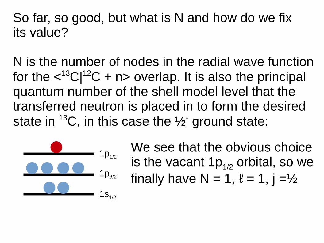
So far, so good, but what is N and how do we fixits value?

N is the number of nodes in the radial wave functionfor the <13C|12C + n> overlap. It is also the principalquantum number of the shell model level that thetransferred neutron is placed in to form the desiredstate in 13C, in this case the ½- ground state:

1s1/2

1p3/2

1p1/2We see that the obvious choiceis the vacant 1p1/2 orbital, so we finally have N = 1, ℓ = 1, j =½

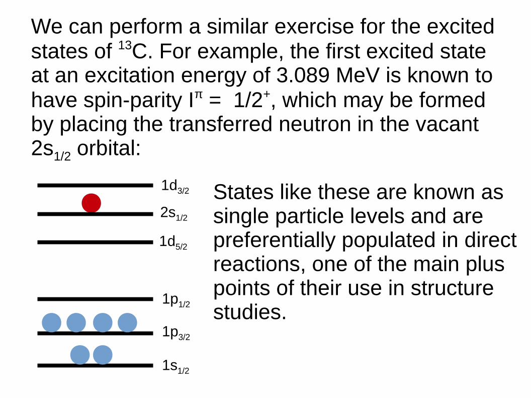
We can perform a similar exercise for the excitedstates of 13C. For example, the first excited stateat an excitation energy of 3.089 MeV is known to have spin-parity Iπ = 1/2+, which may be formedby placing the transferred neutron in the vacant2s1/2 orbital:

1s1/2

1p3/2

1p1/2

1d5/2

2s1/2

1d3/2 States like these are known assingle particle levels and arepreferentially populated in directreactions, one of the main pluspoints of their use in structurestudies.

Finally, to calculate the wave function for the<13C|12C + n> overlaps we need to specify a12C + n binding potential. This is usually a (real)Woods-Saxon well with some radius and diffuseness parameters, plus a spin-orbit part.

By convention the spin-orbit term has the sameradius and diffuseness as the central Woods-Saxonwell and is of the Thomas type we encountered when we considered the optical model. It has a fixeddepth (often around 5-6 MeV).

The central well-depth is adjusted so that the bindingenergy obtained is equal to the experimental value.

How do we choose the values for the radius anddiffuseness parameters? This is an important point,as we shall see in the next lecture.

In practice, the choice is somewhat arbitrary. Commonvalues are: R = 1.25 x A1/3 fm, a = 0.65 fm. There isno real physical justification for these time honouredvalues but they give reasonable results.

With the “geometry” of the binding potential fixed(and the spin-orbit term also fixed) and the N ℓ j valuesspecified the reaction code will search on the welldepth to give the correct binding energy.

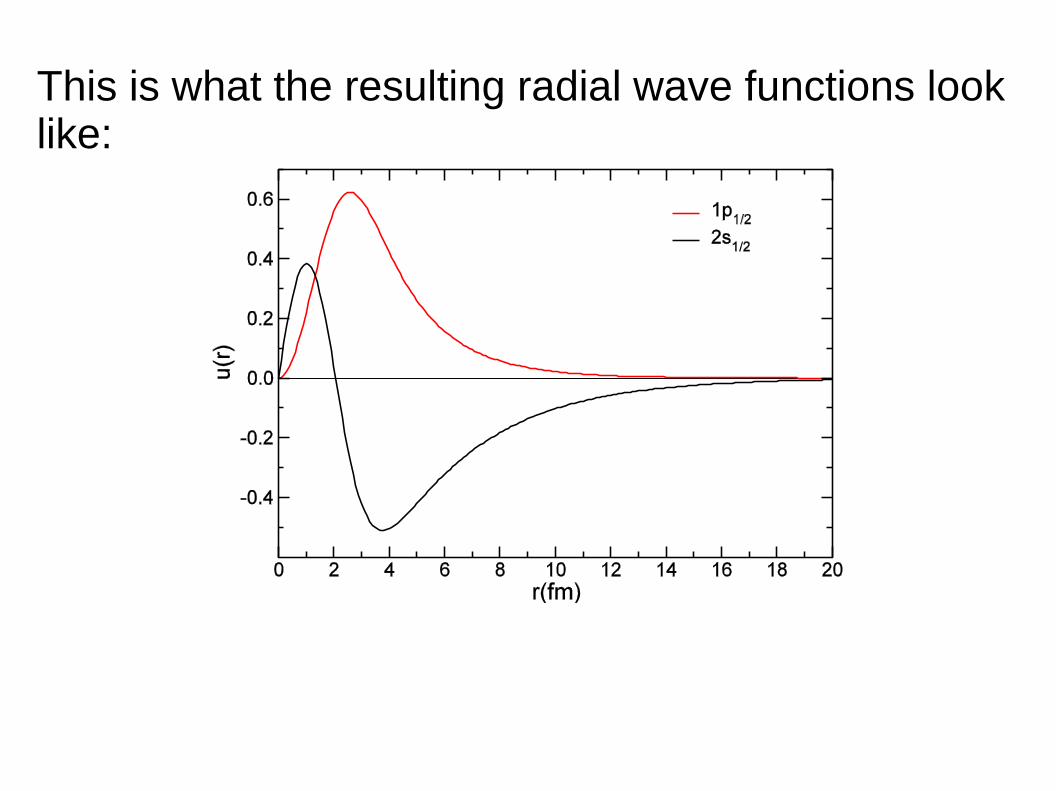
This is what the resulting radial wave functions look like:

We must carry out the same exercise for theprojectile-like overlap, in our example: <d|n + p>.

These overlaps (for light-ion induced reactions)are known, either empirically (from analyses oflarge sets of data) or theoretically (calculated usingtheoretical wave functions from structure theory).

In zero-range DWBA the projectile-like overlap isreduced to a normalisation factor D0. Values ofD0 are well known for (d,p), (d,n), (p,d) and (n,d)reactions, less well known for (d,t) and (d,3He) andvery imperfectly known for reaction like (3He,4He).

For finite-range DWBA the full wave functions arerequired, as for the target-like overlaps. Again,these are well known for (d,p) etc. reactions butless well defined for others (for heavy ion projectileswe use the same procedure as for the target overlaps).

We now have all the ingredients we need to performa DWBA calculation and we shall look at how this isdone in detail in the next lecture, continuing with the12C(d,p)13C reaction as our example.

Lecture 10: transfer reactions continued

In this lecture we shall look at how a DWBA analysisis performed in reality, taking the 12C(d,p)13C reactionat E

d = 30 MeV as our example.

Good data exist at this energy from Ohnuma et al.,Nucl. Phys. A 448 (1986) 205. We will look at transferto four states in 13C: the 0.0 MeV 1/2−, the 3.09 MeV 1/2+, the 3.68 MeV 3/2− and the 3.85 MeV 5/2+.

For direct, one-step transfer these states representa neutron in the 1p

1/2, 2s

1/2, 1p

3/2 and 1d

5/2 shell model

orbitals outside the 12C 0+ core.

In this case the spins and parities of the final statesare all known, so calculating the wave functionsfor the <13C|12C + n> overlaps is simple. We just need to choose the following:

1) An entrance channel d + 12C OMP

2) Exit channel p + 13C OMPs (since the energy of the proton ejectile will be a function of E

x of the

final state in 13C)

3) n + 12C and n + p binding potential parameters for finite range DWBA, D

0 for zero range

For 1) and 2) we simply take the same potentialsas in the original analysis of Ohnuma et al. (oftenthe energy dependence of the exit channel OMPis ignored and we use that for E

x = 0 MeV)

For the n + 12C binding potentials, we assume aWoods-Saxon shape and radius parameters ofR = 1.25 x 121/3 fm, diffusenesses a = 0.65 fm,plus a spin-orbit term of Thomas form with a depthof 6.0 MeV.

The depth of the central Woods-Saxon well is automatically adjusted by our DWBA code – FRESCO here – to give us the correct binding energies

For the n + p binding potential in finite range DWBAwe use that due to Reid, Ann. Phys. (N.Y.) 50, 441 (1968). This gives a realistic deuteron wave function,including the small D state component.

For zero range DWBA we take D0 = 1.55 x 104 MeV fm3

and a finite range correction factor of 0.621 fm, apopular choice since it is given as an example in theDWUCK4 manual (a zero range DWBA code).

How do finite range and zero range DWBA comparewith each other and the data?

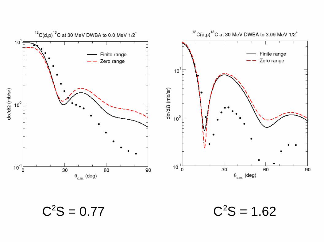
C2S = 0.77 C2S = 1.62

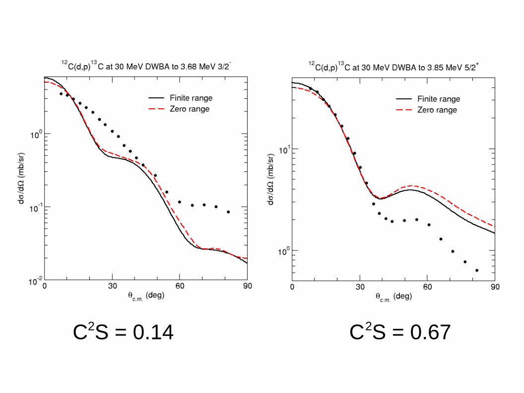
C2S = 0.14 C2S = 0.67

While zero range and finite range give similar results – the spectroscopic factors (C2S) are the same forboth calculations in each case – it has to be saidthat they do not reproduce the measured ADs very well. This could be for multiple reasons:

1) Our choice of OMP in entrance and exit channel

2) Our choice of binding potential parameters

3) DWBA is not an adequate theory here, the reaction mechanism is more complicated than simple one- step transfer

Leaving aside 3) for the present (although the C2Svalues suggest that it may be relevant, since none ofthem are particularly close to 1.0, the expected valuefor a pure single particle state) let us consider 1).

There are no d + 12C elastic scattering data at 30 MeVbut there are some at E

d = 29.5 MeV – close enough!

How well are they described by our OMP?

The answer is not too bad, but could do much better!

We should be able to improve on the description ofthe d + 12C elastic scattering, but will this affect the12C(d,p)13C results?

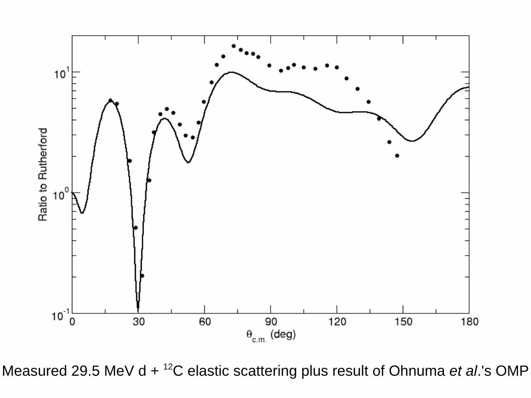
Measured 29.5 MeV d + 12C elastic scattering plus result of Ohnuma et al.'s OMP

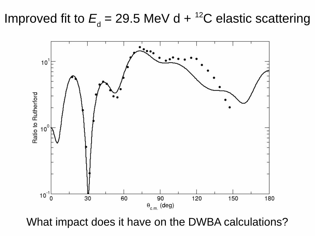
Improved fit to Ed = 29.5 MeV d + 12C elastic scattering

What impact does it have on the DWBA calculations?

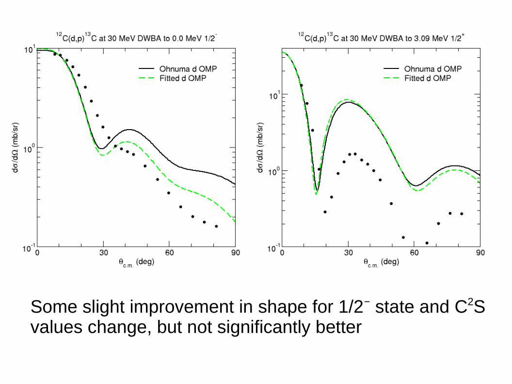
Some slight improvement in shape for 1/2− state and C2Svalues change, but not significantly better

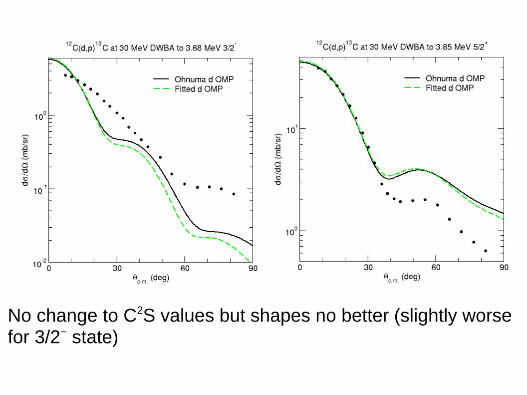
No change to C2S values but shapes no better (slightly worse for 3/2− state)

Thus, the general conclusion is that the DWBAdescription of the 12C(d,p)13C data is not improved by a better description of the entrance channel elastic scattering

What about the exit channel? There are data forelastic scattering of 30.4 MeV protons from 13C,close to the energy of the exit channel for populatingthe 13C 1/2− ground state

What effect does replacing the exit channel OMP ofOhnuma et al. have on the DWBA? We retain the“best fit” d + 12C OMP in the entrance channel …

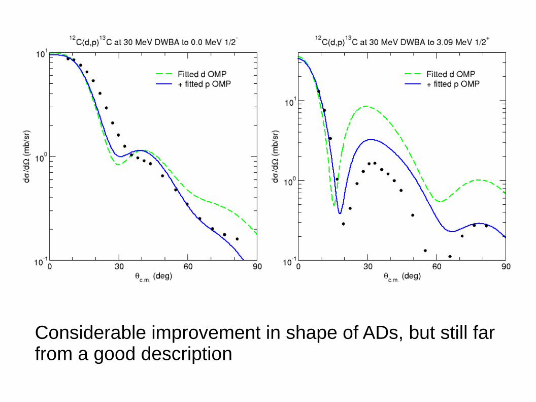
Considerable improvement in shape of ADs, but still far from a good description

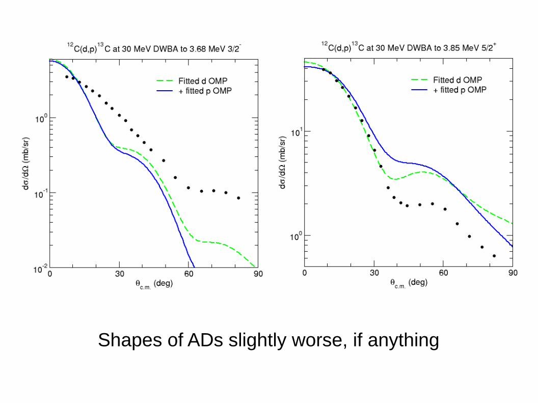
Shapes of ADs slightly worse, if anything

A general conclusion for this case seems to be that we can obtain some improvement by using OMPsthat give a better description of the relevant elasticscattering (here mostly the exit channel) but we arestill some way from a satisfactory description.

Let us now consider point 2), the binding potentialparameters. We consider just the target-like case,since the projectile overlap is well-known (and in thezero range case is reduced to a normalisation factoranyway, D

0).

What effect does changing r0 over a reasonable

range have? Investigate effect of r0 = 1.0 and 1.5 fm

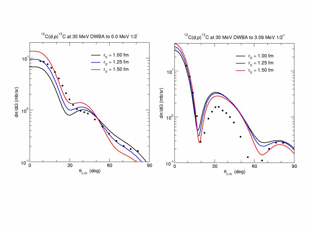
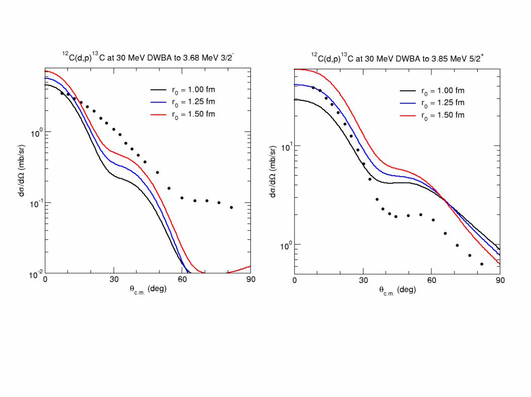
Only in the case of the 5/2+ state is the shape ofthe AD improved. The main effect in each case isto change the magnitude of the cross section, i.e.the spectroscopic factor.

This is in fact a general problem, since one of themain pieces of information that we wish to extractfrom direct reaction data of this type is the C2Svalue. Since it is rather sensitive to the choice ofr

0 and we do not have a reliable way of fixing this

parameter the uncertainties can be large …

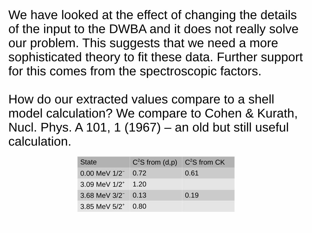
We have looked at the effect of changing the detailsof the input to the DWBA and it does not really solveour problem. This suggests that we need a moresophisticated theory to fit these data. Further supportfor this comes from the spectroscopic factors.

How do our extracted values compare to a shellmodel calculation? We compare to Cohen & Kurath,Nucl. Phys. A 101, 1 (1967) – an old but still usefulcalculation.

State C2S from (d,p) C2S from CK

0.00 MeV 1/2− 0.72 0.61

3.09 MeV 1/2+ 1.20

3.68 MeV 3/2− 0.13 0.19

3.85 MeV 5/2+ 0.80

Agreement is reasonable, given the poor descriptionof the ADs by DWBA (CK did not calculate the C2Svalues for the positive parity states since their modelonly allowed states up to the p-shell).

What is significant is that the 3/2− state has a smallC2S, much smaller than 1.0. This is therefore notwell described as a neutron in a shell model leveloutside the 12C core in its ground state.

A glance at the shell model scheme explains this:

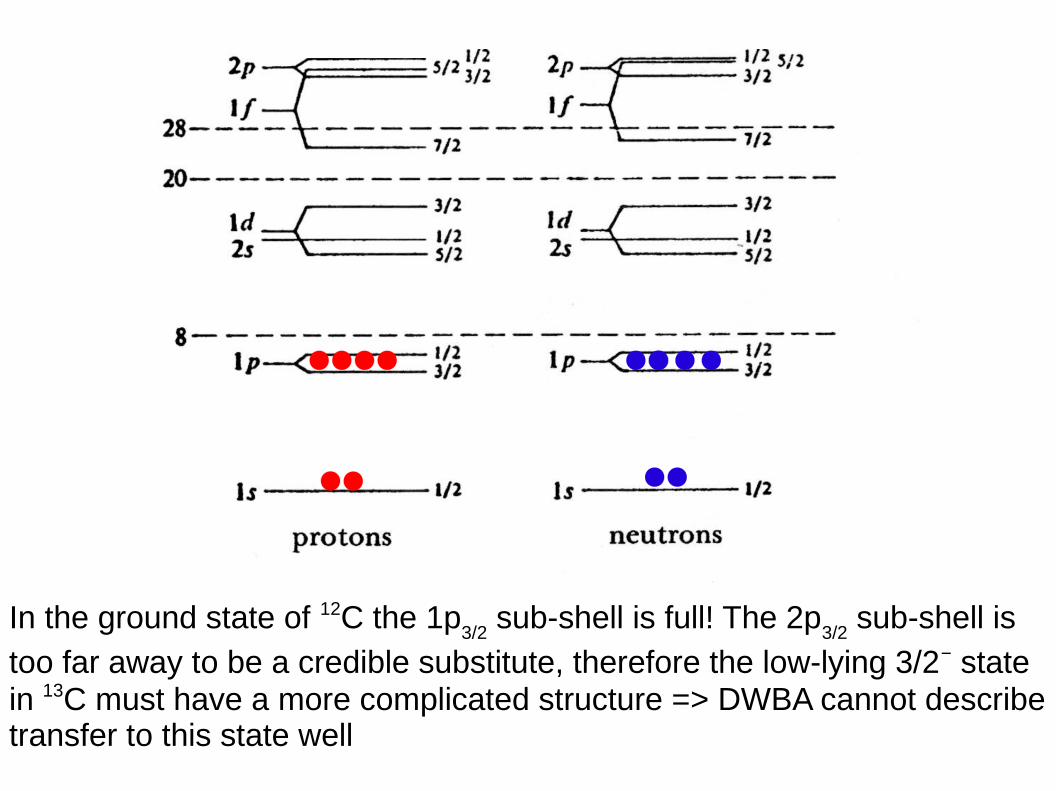
In the ground state of 12C the 1p3/2

sub-shell is full! The 2p3/2

sub-shell is

too far away to be a credible substitute, therefore the low-lying 3/2− statein 13C must have a more complicated structure => DWBA cannot describetransfer to this state well

The poor description of the 3/2− state by the DWBAis thus explained by its structure; there is littleoverlap between the ground state of 12C and thisstate in 13C.

Therefore, to describe this state (and the better todescribe the other states) we need to use a moresophisticated theory of the reaction which will allowthe inclusion of 2-step (or more) reaction paths, e.g.excitation of the 4.44 MeV 2+ state in 12C followedby transfer of a neutron to form states with structureslike: <13C|12C* + n>

To do this we need to use the coupled channelsBorn approximation (CCBA) or the coupled reactionchannels (CRC) formalisms. We shall look at thesenext week. We will also briefly consider the rôle ofthe weak binding energy of the deuteron and how itcan be taken into account.

Finally for this lecture, a word about spectroscopicfactors.

You will have noticed that I have used the label “C2S”in the text of this lecture to denote the spectroscopicfactor; why have I done so and what is this mysterious C?

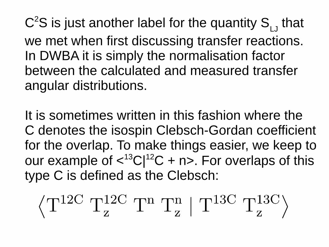
C2S is just another label for the quantity SLJ

thatwe met when first discussing transfer reactions.In DWBA it is simply the normalisation factorbetween the calculated and measured transferangular distributions.

It is sometimes written in this fashion where theC denotes the isospin Clebsch-Gordan coefficientfor the overlap. To make things easier, we keep toour example of <13C|12C + n>. For overlaps of thistype C is defined as the Clebsch:

T and Tz are well known for the neutron: T = T

z = ½

For 12C and 13C, Tz is easily calculated by the

following relation:

Tz = (N − Z)/2

This applies to all nuclei (N.B. the sign conventionsfor T

z are as used in nuclear physics).

For T, we must look it up for the state in question.For light nuclei, the following site gives the values:

http://www.tunl.duke.edu/nucldata/

For 12C, Tz = 0 and we find that T = 0 too for the

ground state.

For 13C, Tz = (7 − 6)/2 = ½ and we find that T = ½

too for all the states we are considering

We therefore need the following Clebsch:

< 0 0 ½ ½ | ½ ½>

These are tabulated and there are also on-linecalculators, e.g.

http://personal.ph.surrey.ac.uk/~phs3ps/cgjava.html

In this case, C = 1.0 so C2S = S. It is not always so,and C is often < 1.0.

Why bother with this extra complication since thenumber we extract from our data is C2S anyway?

Simply that often calculated spectroscopic factorsare just S and do not contain the C2 factor (this isthe case for the Cohen and Kurath values citedearlier) so if we wish to compare our empirical valueswith, say, the shell model then we need to be awareof this and calculate the relevant C2.

In the next lecture, more sophisticated reaction theories.

Lecture 11: transfer reactions continued

We saw last time how DWBA was unable to providea satisfactory description of the 12C(d,p)13C reactionat E

d = 30 MeV.

This suggests a more complicated reaction mechanism than the simple, single step weak process supposed by DWBA.

We saw that at least in one case (the 3/2− excited state)the shell model level sequence supports this possibilitysince the 1p

3/2 level is already full in 12C.

There are two main possible sources of complex, i.e. more than single step, reaction paths in the d + 12Csystem:

i) 12C has a strongly coupled excited state (2+) at E

x = 4.44 MeV. We can envisage excitation of this

state followed by transfer as a two step process

ii) the deuteron is weakly bound (Sn = S

p = 2.22 MeV)

so breaks up easily. This process can interfere with the (d,p) transfer so absorbing its effect into the OMP may not be adequate

Of course, both these effects may contribute …

We begin by looking at the first possibility, inelasticexcitation followed by transfer. How do we handle it?

The simplest way is to retain DWBA for the transferstep and to use coupled channels theory for theinelastic scattering step. This is known as the CoupledChannels Born Approximation, or CCBA

We use CC for the inelastic excitation since it isstrong (therefore DWBA not in principle suitable) andretain DWBA for the transfer as it is assumed weak

How can we visualise CCBA versus DWBA?

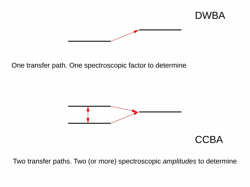
DWBA

CCBA

One transfer path. One spectroscopic factor to determine

Two transfer paths. Two (or more) spectroscopic amplitudes to determine

Before considering the extra ingredients neededin CCBA compared to DWBA we should explainwhat we mean by a spectroscopic amplitude inthis context and why there could be more than two(surely two transfer paths, two amplitudes?)

First of all, the spectroscopic amplitudes (SA) arethe square roots of the spectroscopic factors wemet last time, i.e. SA = √(C2S)

They are therefore signed (can be +ve or −ve) andthe signs matter since we may have interferencebetween different reaction paths

Secondly, we may have more than two of them to determine here thanks to our old friends the rules for angular momentum addition in quantum mechanics

As an illustration, take 12C(d,p)13C to the 3.68 MeV3/2− state of 13C. As we saw last time, for transferonto the 0+ state of the 12C core the neutron canonly occupy a p

3/2 shell model level. Since the core

spin Jcore

was 0 it didn't enter consideration.

For the two step path, Jcore

= 2, so we now have to“couple” to the core spin too when we determine whichshell model levels can give us a 3/2− state in the final13C nucleus.

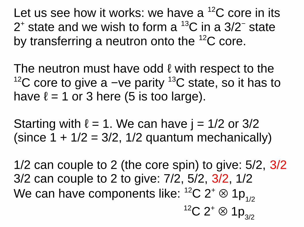
Let us see how it works: we have a 12C core in its2+ state and we wish to form a 13C in a 3/2− state by transferring a neutron onto the 12C core.

The neutron must have odd ℓ with respect to the12C core to give a −ve parity 13C state, so it has to have ℓ = 1 or 3 here (5 is too large).

Starting with ℓ = 1. We can have j = 1/2 or 3/2 (since 1 + 1/2 = 3/2, 1/2 quantum mechanically)

1/2 can couple to 2 (the core spin) to give: 5/2, 3/2 3/2 can couple to 2 to give: 7/2, 5/2, 3/2, 1/2We can have components like: 12C 2+ 1p

1/2

12C 2+ 1p3/2

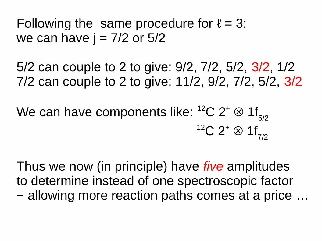
Following the same procedure for ℓ = 3:we can have j = 7/2 or 5/2

5/2 can couple to 2 to give: 9/2, 7/2, 5/2, 3/2, 1/27/2 can couple to 2 to give: 11/2, 9/2, 7/2, 5/2, 3/2

We can have components like: 12C 2+ 1f5/2

12C 2+ 1f7/2

Thus we now (in principle) have five amplitudesto determine instead of one spectroscopic factor − allowing more reaction paths comes at a price …

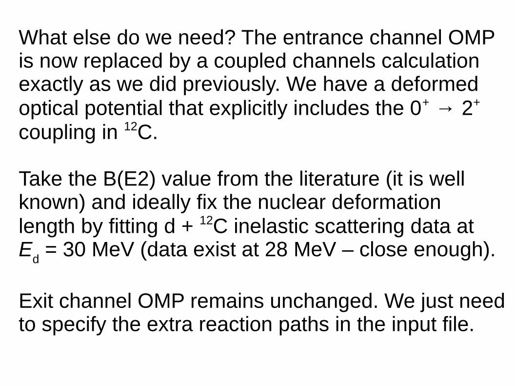
What else do we need? The entrance channel OMPis now replaced by a coupled channels calculationexactly as we did previously. We have a deformedoptical potential that explicitly includes the 0+ → 2+

coupling in 12C.

Take the B(E2) value from the literature (it is well known) and ideally fix the nuclear deformation length by fitting d + 12C inelastic scattering data at E

d = 30 MeV (data exist at 28 MeV – close enough).

Exit channel OMP remains unchanged. We just needto specify the extra reaction paths in the input file.

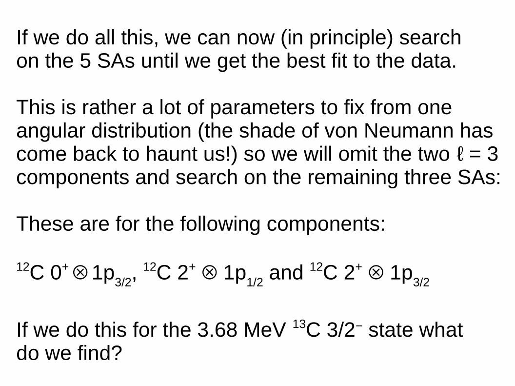
If we do all this, we can now (in principle) search on the 5 SAs until we get the best fit to the data.

This is rather a lot of parameters to fix from oneangular distribution (the shade of von Neumann hascome back to haunt us!) so we will omit the two ℓ = 3components and search on the remaining three SAs:

These are for the following components:

12C 0+ 1p3/2

, 12C 2+ 1p1/2

and 12C 2+ 1p3/2

If we do this for the 3.68 MeV 13C 3/2− state what do we find?

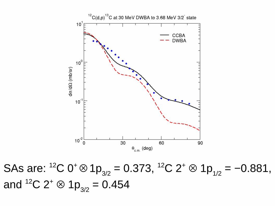
SAs are: 12C 0+ 1p3/2

= 0.373, 12C 2+ 1p1/2

= −0.881,

and 12C 2+ 1p3/2

= 0.454

We see that the CCBA fit to the data is much better(at the price of an additional two adjustable parameterswith all that this implies) and in this case the SA for the12C 0+ 1p

3/2 component has not changed.

However, the reproduction is still far from perfect: thecalculated AD is too structured compared to themeasured one.

This could be due to the missing ℓ = 3 components,components built on other excited states of the 12Ccore (e.g. the 9.63 MeV 3−) or the effect of deuteronbreakup.

This provides a convenient point to consider thequestion of how the effects of deuteron breakupmay be explicitly included in a transfer calculation.

The simplest way is to use the adiabatic model.[Johnson and Soper, Phys. Rev. C 1 (1970) 976, Harvey and

Johnson, Phys. Rev. C 3 (1971) 636]

This model keeps the DWBA formalism but thedeuteron distorted wave (entrance channel for (d,p)or exit channel for (p,d) reactions) is redefined. Itstill describes the motion of the centre of mass of the neutron and proton but they may no longer be in the form of a bound deuteron.

This is done by introducing an adiabatic potentialinto a standard DWBA code in lieu of the usualdeuteron OMP. The potential is adiabatic becauseit ignores the “excitation energy” of the deuteroncompared to its incident energy.

We will not discuss how the adiabatic potential iscalculated here, but there are approximationsavailable that make it a simple job.

Therefore, the adiabatic model should work bestfor higher incident energies. In fact, it is found towork well even at fairly low E

d values, due to the

errors in the assumptions largely cancelling eachother out.

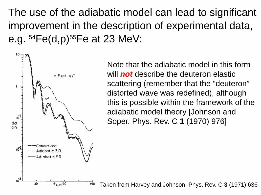
Taken from Harvey and Johnson, Phys. Rev. C 3 (1971) 636

Note that the adiabatic model in this formwill not describe the deuteron elasticscattering (remember that the “deuteron”distorted wave was redefined), although this is possible within the framework of theadiabatic model theory [Johnson and Soper. Phys. Rev. C 1 (1970) 976]

The use of the adiabatic model can lead to significant improvement in the description of experimental data, e.g. 54Fe(d,p)55Fe at 23 MeV:

The disadvantage of the adiabatic model is thatit can only be used as a replacement for DWBA;it cannot be adapted to CCBA scenarios. Also, itis not suitable for use within the coupled reactionchannels (CRC) formalism, which we shall discusspresently.

A more accurate theory for the modelling of breakupexists, known as the coupled discretised continuumchannels (CDCC) method, due to Rawitscher, Phys.Rev. C 9, 2210 (1974). We will not go into detailshere, but suffice it to say that it is an extension of thestandard CC theory to include couplings to thecontinuum.

CDCC can be used to model the deuteron breakupin a CCBA-type calculation (target excitation can beincluded) and is also suitable for use in a CRCcalculation.

It can also be used in other reactions involving deuterons such as (d,t), (d,3He), (d,6Li) etc., whichthe adiabatic model can not.

CDCC is therefore more flexible than the adiabaticmodel but requires much more computing time sincethe continuum couplings are explicitly included in aCC type calculation (and there are usually many ofthem).

The final refinement that we can make in our reactionmodel is to treat the transfer step(s) on the samefooting as the other couplings, i.e. no longer treatthem as weak so that they can be handled withperturbation theory, as in DWBA.

To do this we use so-called coupled reaction channelsor CRC. In principle this is CC theory with the extracomplication that the exit channel now belongs to adifferent partition.

In practice it is handled by iterating a series of DWBA steps until the result converges, since “full” CRC would be very computationally intensive (the two methods give identical results).

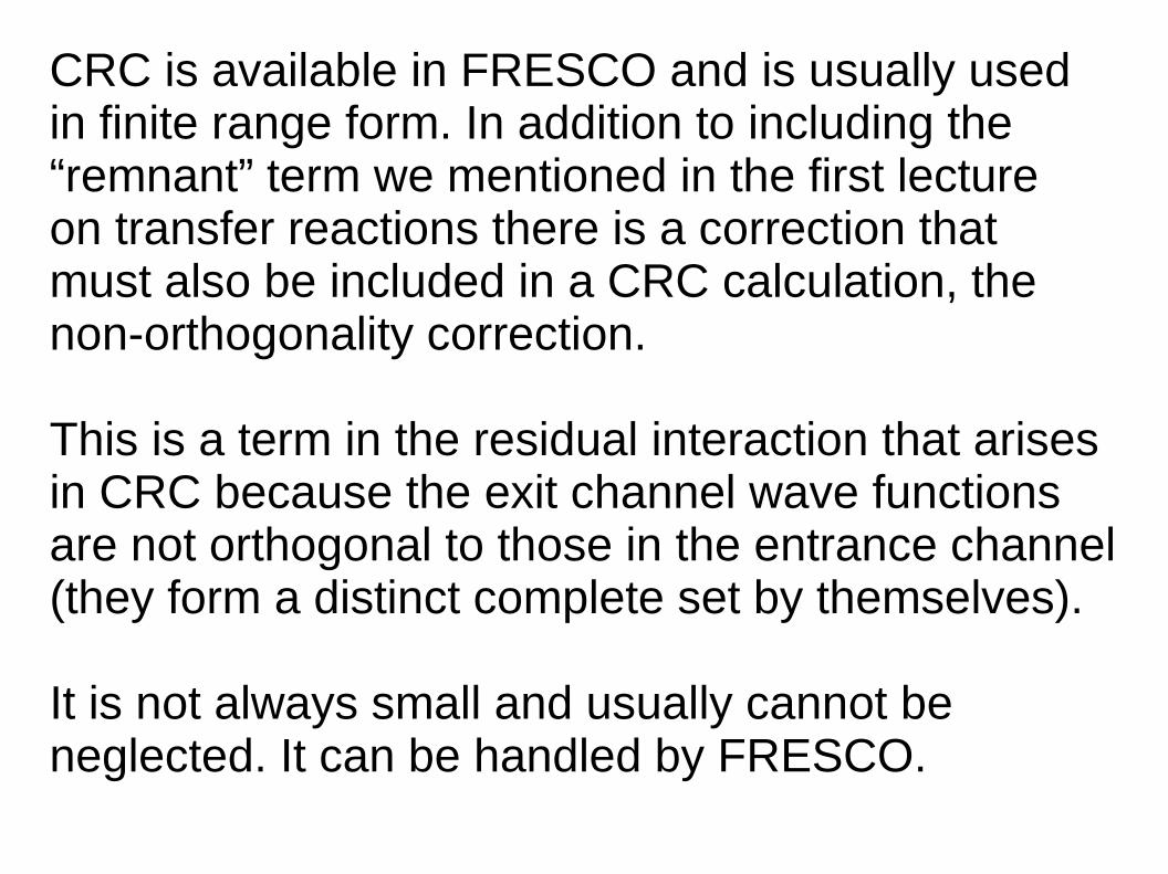
CRC is available in FRESCO and is usually usedin finite range form. In addition to including the“remnant” term we mentioned in the first lectureon transfer reactions there is a correction thatmust also be included in a CRC calculation, thenon-orthogonality correction.

This is a term in the residual interaction that arisesin CRC because the exit channel wave functionsare not orthogonal to those in the entrance channel(they form a distinct complete set by themselves).

It is not always small and usually cannot be neglected. It can be handled by FRESCO.

Putting it all together: keeping to our 12C(d,p)13Cexample how well can we describe these datausing the most sophisticated model of the reactionmechanism we have available?

This is CC for the inelastic excitation of the 12C2+ state, CDCC for deuteron breakup and CRC for transfer steps, including two step via the 12C2+ state.

How well does all this apparatus work in reality?

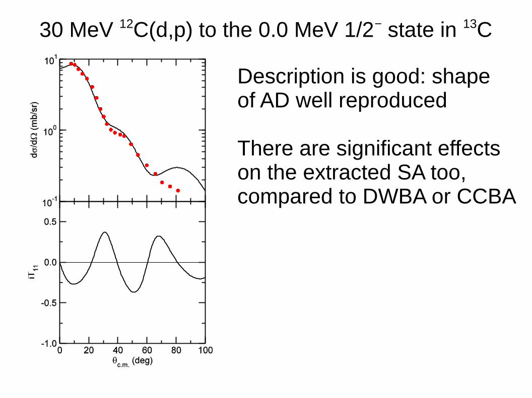
30 MeV 12C(d,p) to the 0.0 MeV 1/2− state in 13C

Description is good: shapeof AD well reproduced

There are significant effectson the extracted SA too,compared to DWBA or CCBA

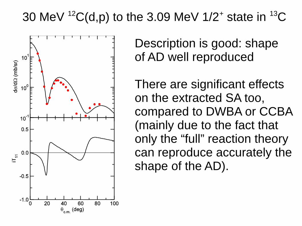
30 MeV 12C(d,p) to the 3.09 MeV 1/2+ state in 13C

Description is good: shapeof AD well reproduced

There are significant effectson the extracted SA too,compared to DWBA or CCBA(mainly due to the fact thatonly the “full” reaction theorycan reproduce accurately theshape of the AD).

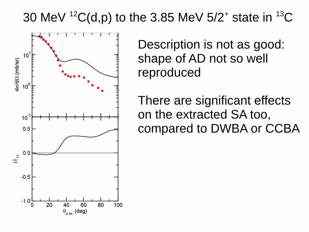
30 MeV 12C(d,p) to the 3.85 MeV 5/2+ state in 13C

Description is not as good: shape of AD not so well reproduced

There are significant effectson the extracted SA too,compared to DWBA or CCBA

We see that the “full” model of the reaction in general leads to a much improved description ofthe data (there are still problems with the 5/2+ state)

Not only are the shapes of the ADs better reproducedbut there are also significant changes in the spectroscopic amplitudes (or factors) that we extractfrom the normalisation of the theory curves to thedata.

Thus, failure of DWBA to describe transfer data canindicate real physics – it may mean that we need touse a more sophisticated reaction model becausethe assumptions underlying DWBA are no longer valid

However, to avoid giving you the wrong impression,DWBA works very well when the conditions arefulfilled. As a case study, we take the 124Sn(d,p)125Snreaction at E

d = 9 MeV.

These data also provide a good example of “typical” radioactive beam data (although 124Sn is effectively stable these data were taken in inverse kinematics as a test of a RIB set-up and analysis techniques).

Data from: Jones et al., Phys. Rev. C 70 (2004) 067602

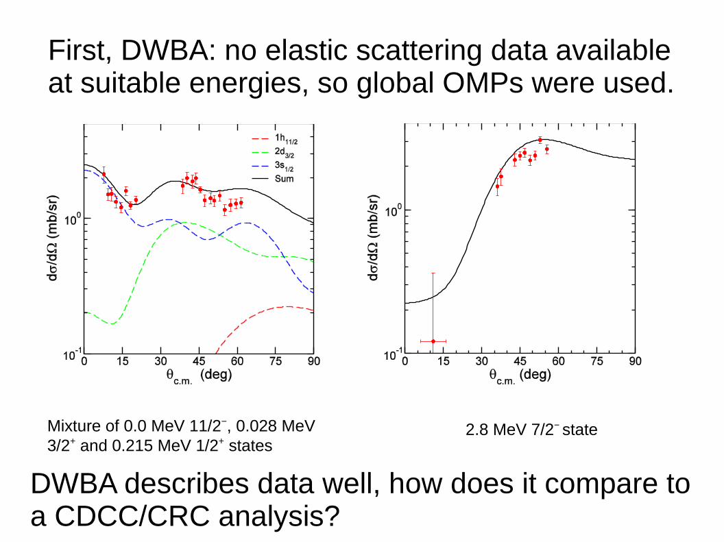
First, DWBA: no elastic scattering data availableat suitable energies, so global OMPs were used.

Mixture of 0.0 MeV 11/2−, 0.028 MeV3/2+ and 0.215 MeV 1/2+ states

2.8 MeV 7/2− state

DWBA describes data well, how does it compare toa CDCC/CRC analysis?

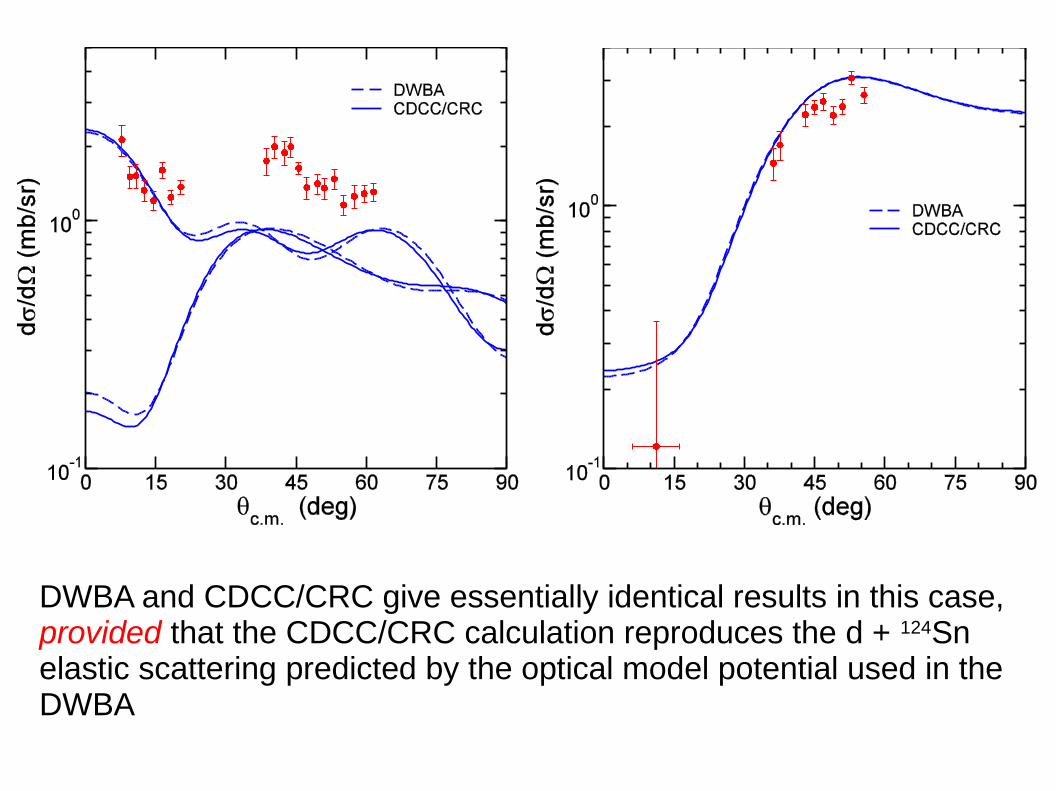
DWBA and CDCC/CRC give essentially identical results in this case, provided that the CDCC/CRC calculation reproduces the d + 124Sn elastic scattering predicted by the optical model potential used in the DWBA

Finally, a word about spectroscopic factors/amplitudes

We saw in the first lecture on transfers that the shapeof the angular distribution can give us the ℓ value of thefinal state, an important piece of information (it placeslimits on the spin of the state).

Another useful piece of information is the spectroscopicfactor. As we said earlier, it should always be borne inmind that this is not an observable and is thereforemodel dependent.

We have seen that the exact value obtained can depend on the reaction model used.

It is also sensitive to the binding potentials usedto bind the transferred particle to the core nucleus.It is most sensitive to the radius of this potential,which is not usually fixed with any degree ofcertainty.

In CCBA and CRC we may also have to determineseveral spectroscopic amplitudes from a single AD,so the situation is even worse.

However, we can distinguish with certainty betweensmall and large spectroscopic factors, so we cansay which states are good single particle levels

As usual in direct reaction work, we must be carefulabout making detailed comparisons of absolutenumbers extracted from experiment using somemodel with what is calculated by a structure theory:they are not necessarily the same thing!

In the final lecture we consider transfer reactionsinduced by heavy ions and why they are interesting.

Lecture 12: heavy ion induced transfer reactions

The previous two lectures have concentrated ontransfer reactions induced by light ions. We haveseen that such reactions are important sources ofnuclear structure information due to their selectivity (preferential population of single-particlestates).

In this final lecture we shall look at transfer reactionsinduced by heavy ions. Here the motivation is ratherdifferent since we are mainly concerned with thereaction mechanism and the effect of such couplingson the elastic scattering.

It is possible to use heavy ion induced transferreactions for spectroscopy, but this is not oftendone due to the need to fix the “projectile-like”spectroscopic factor(s)/wave functions as wellas the “target-like” (usually the ones of interest).

e.g. 208Pb(12C,11B)209Bi could be used to look at “single proton” levels in 209Bi instead of the (3He,d) reaction but the <12C|11B+p> overlap is much less well known than the <3He|d+p> one.

There can be advantages to using heavy ion projectiles though, due to Q matching

Heavy ion induced transfer reactions are observedto have a strong dependence on the Q value ofthe reaction. This Q-window effect is due to therequirement that for maximum transfer amplitudethe orbits of the incoming and outgoing particlesbefore and after the transfer are continuous.

This means that for a given reaction there is anoptimum Q value that favours it. For neutrontransfers this is always 0 MeV. For proton transfersit is negative for stripping (as in our (12C,11B) example)and positive for pickup (e.g. the (12C,13N) reaction).

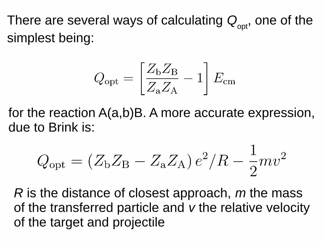
There are several ways of calculating Qopt

, one of the simplest being:

for the reaction A(a,b)B. A more accurate expression,due to Brink is:

R is the distance of closest approach, m the mass of the transferred particle and v the relative velocityof the target and projectile

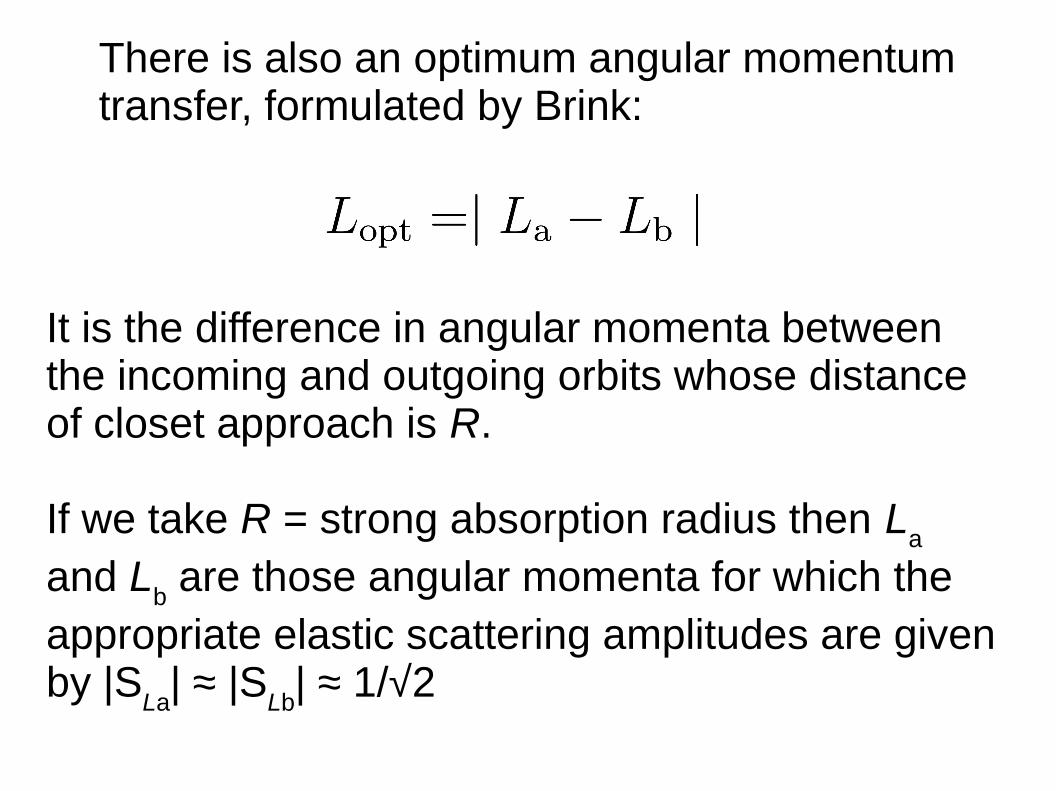
There is also an optimum angular momentumtransfer, formulated by Brink:

It is the difference in angular momenta betweenthe incoming and outgoing orbits whose distanceof closet approach is R.

If we take R = strong absorption radius then La

and Lb are those angular momenta for which the

appropriate elastic scattering amplitudes are given by |S

La| ≈ |S

Lb| ≈ 1/√2

These matching conditions mean that with carefulchoice of the projectile it is possible preferentially topopulate particular levels with heavy ion reactions.

This can be useful for spectroscopic purposes, butas we said previously, it is difficult to extract absolute spectroscopic factors from such reactions.

The relative C2S value are fairly well fixed, sincethe normalisation of calculation to data fixes theproduct S

aS

A and S

a is the same for all transitions,

so the relative values should match well with those obtained from light ion reactions.

Turning now to a practical example, we choose the208Pb(12C,11B)209Bi single proton stripping reactionat an incident energy of 97.9 MeV.

Data for this reaction exist for 5 states in 209Bi:0.0 MeV 9/2−, 0.90 MeV 7/2−, 1.61 MeV 13/2+,2.84 MeV 5/2− and 3.12 MeV 3/2−. There are alsodata for the elastic scattering in the entrance andexit channels at suitable energies.

We first repeat the original DWBA analysis inK. S. Toth et al., Phys. Rev. C 14 1471 (1976).

Entrance and exit channel distorted waves arecalculated using the OMP parameters given inthe original paper. We do the same thing for thebound state wave functions for the projectile andtarget overlaps.

For the projectile overlap the procedure is one thatis found to work well for light, p-shell projectiles.We take the calculated spectroscopic factors ofCohen and Kurath, Nucl. Phys. A 101, 1 (1967) and use a Woods-Saxon well of radius 1.25 x A1/3

and diffuseness 0.65 fm.

N.B. here C2 ≠ 1 since the isospin Clebsch-Gordan coefficient for 12C = 11B + p is 1/√2

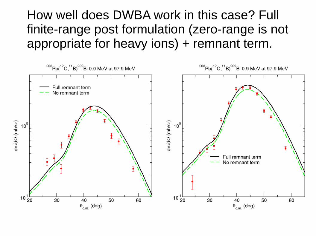
How well does DWBA work in this case? Fullfinite-range post formulation (zero-range is notappropriate for heavy ions) + remnant term.

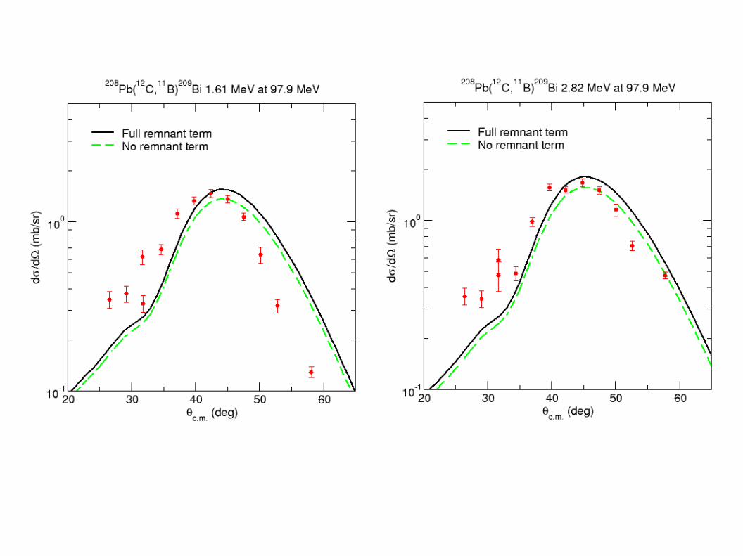
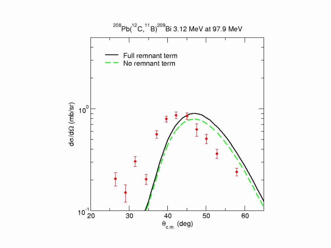
The overall description is reasonable, althoughthere are a few things to note:

1) If we use the full remnant term post and prior give identical results

2) Omission of the remnant term makes a significant difference, cf. dashed green and solid black curves

3) There is a systematic shift to larger angles of the calculated transfer peak compared to the measured one (most notable for the 3.12 MeV 3/2− state).

The <209Bi|208Pb+p> spectroscopic factors turnout to be quite reasonable when compared toother measurements and theoretical values, although the latter comparison is always subjective.

However, the discrepancy in the peak positionssuggests some problems with simple DWBA.

It is possible that choice of OMP affects the result,and choice of bound state potential radius may doso too. These possibilities were checked and had little influence on the shape of the transfer ADs.

This suggests that the reaction mechanism may bemore complicated than the simple one-step directassumed in DWBA.

Two-step mechanisms – inelastic excitation ofstates followed by transfer – can be more importantfor heavy ions, since in addition to excitation of thetarget-like nuclei it is now possible to excite theprojectile-like nuclei too.

In the 208Pb(12C,11B)209Bi reaction there are possiblecollective excitations of the 208Pb core (we expectexcitations of 209Bi to be weaker) plus the 12C projectile and 11B ejectile (these should also be weaker)

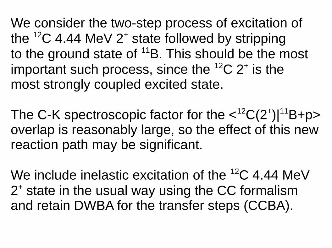
We consider the two-step process of excitation ofthe 12C 4.44 MeV 2+ state followed by strippingto the ground state of 11B. This should be the mostimportant such process, since the 12C 2+ is themost strongly coupled excited state.

The C-K spectroscopic factor for the <12C(2+)|11B+p>overlap is reasonably large, so the effect of this newreaction path may be significant.

We include inelastic excitation of the 12C 4.44 MeV2+ state in the usual way using the CC formalismand retain DWBA for the transfer steps (CCBA).

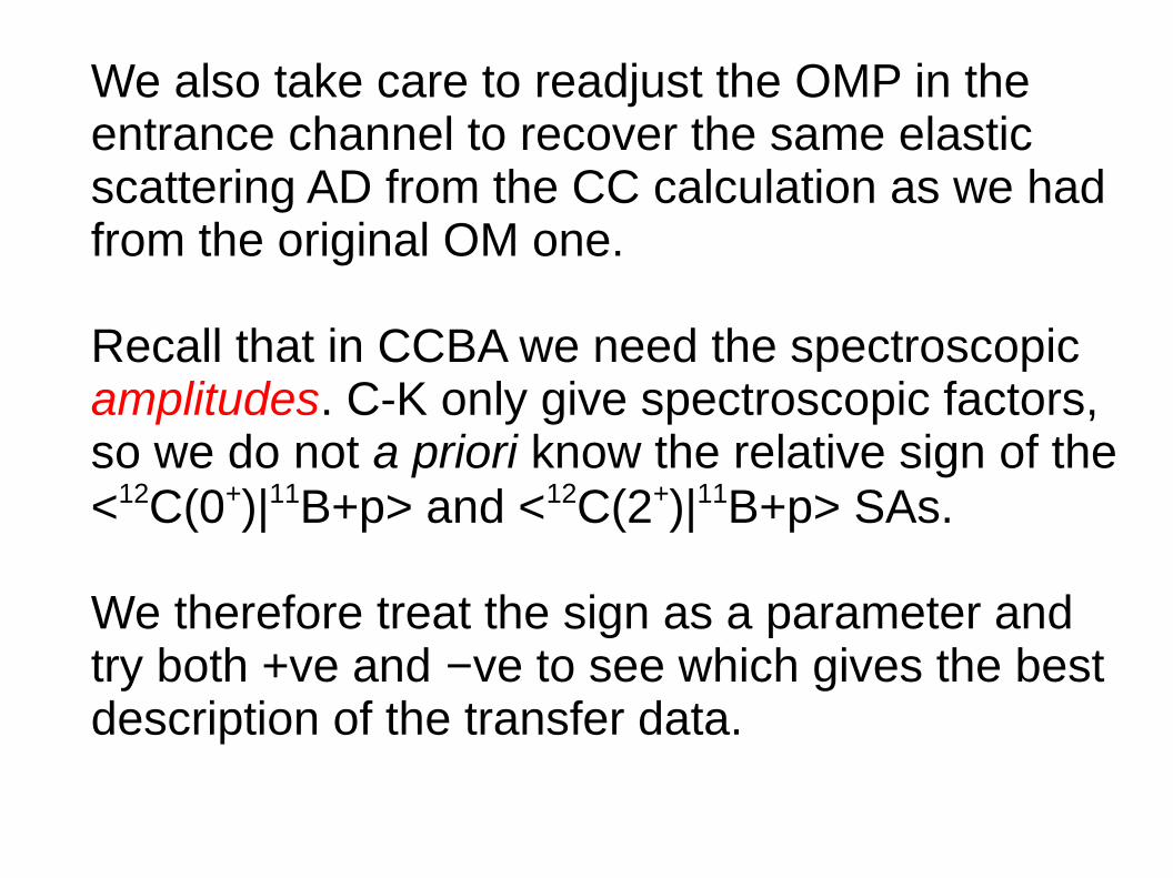
We also take care to readjust the OMP in theentrance channel to recover the same elasticscattering AD from the CC calculation as we hadfrom the original OM one.

Recall that in CCBA we need the spectroscopicamplitudes. C-K only give spectroscopic factors,so we do not a priori know the relative sign of the<12C(0+)|11B+p> and <12C(2+)|11B+p> SAs.

We therefore treat the sign as a parameter andtry both +ve and −ve to see which gives the bestdescription of the transfer data.

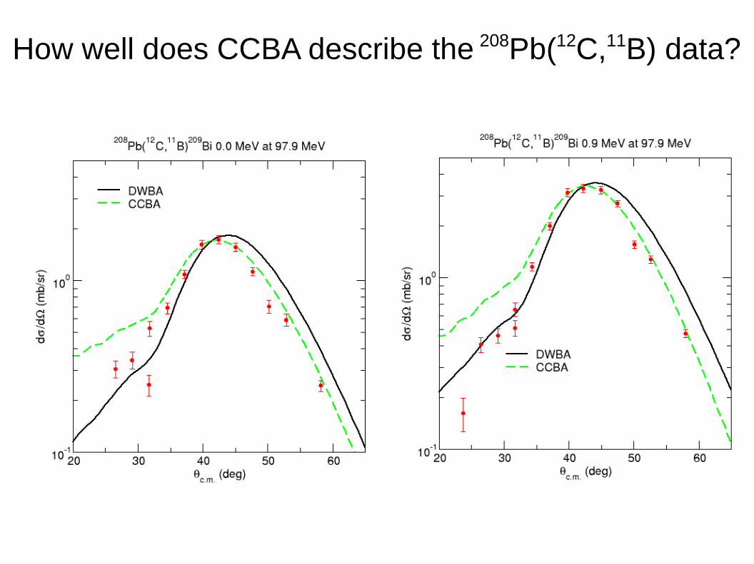
How well does CCBA describe the 208Pb(12C,11B) data?

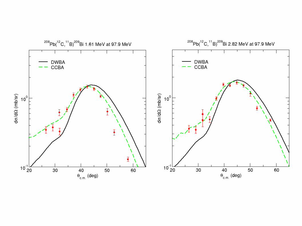
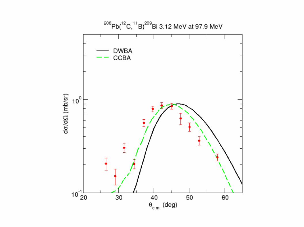
CCBA is able to provide a very good description ofall the data, with the exception of stripping to the3.12 MeV 3/2− state where there is still a mis-matchbetween the position of the measured peak in theAD and the calculated one (but it is much improvedcompared to the DWBA result).

The reaction mechanism does indeed seem to bemore complicated than single-step (and perhapseven three-step or more paths contribute to strippingto the 3.12 MeV 3/2− state).

There are two things to note from this result:

1) Heavy ion transfer reactions can be sensitive to details of the reaction mechanism

2) The relative sign of the <12C(0+)|11B+p> and <12C(2+)|11B+p> spectroscopic amplitudes is unambiguously fixed by this analysis; it must be negative otherwise the peak position shifts to larger angles, i.e. in the wrong direction

We do gain some useful spectroscopic informationfrom this heavy ion transfer after all, in addition to the interest of pinning down the reaction mechanism.

Another motivation for studying heavy ion transferreactions is their possible influence on the elasticscattering. For these studies we must use the CRCtheory, since in both DWBA and CCBA the transferstep is treated as a perturbation and so cannotinfluence the elastic scattering.

We will take as an example some new data for aradioactive beam, 8He, incident on a 208Pb targetat 22 MeV, close to the Coulomb barrier.

Energies close to the Coulomb barrier are wherecoupling effects (of any sort) are most importantfor the elastic scattering.

8He should prove an interesting case. The Q matchingwindow should favour 1n-stripping to low-lying levelsof 209Pb, which are known to be good single-particlelevels.

Also, the <8He|7He+n> and <209Pb|208Pb+n> spectroscopic factors are well known, so a calculationof the 208Pb(8He,7He)208Pb stripping reaction should give a realistic result.

This is an important point since we cannot check theaccuracy of the calculated transfer angular distributions in this case since 7He is unbound (andcoincidence measurements with neutrons are difficult)

There are at least two schools of thought as to how togo about a CRC study of transfer coupling effects onthe elastic scattering:

1) Take a “bare” OMP consisting of a double-folded real part and an imaginary part that simulates absorption due to compound nuclear processes (fusion) only. Then build up all other sources of absorption by coupling explicitly with CC (inelastic) and CRC (transfer) formalisms to all the important channels.

2) Start from the OMP that fits the elastic scattering and readjust its parameters each time you add a coupling to recover the fit.

Both approaches have their merits, and in principleif one could always include all the important channelsin the calculation they would eventually give the sameresults.

In our test case, 8He + 208Pb, we will use the secondapproach since we are interested in the effect ofcoupling to a single process – 1n-stripping – only. The effect of coupling to other channels is absorbedinto the entrance channel OMP.

What does the full CRC calculation look like, and what effect does switching off the 1n-stripping couplings have on the elastic scattering?

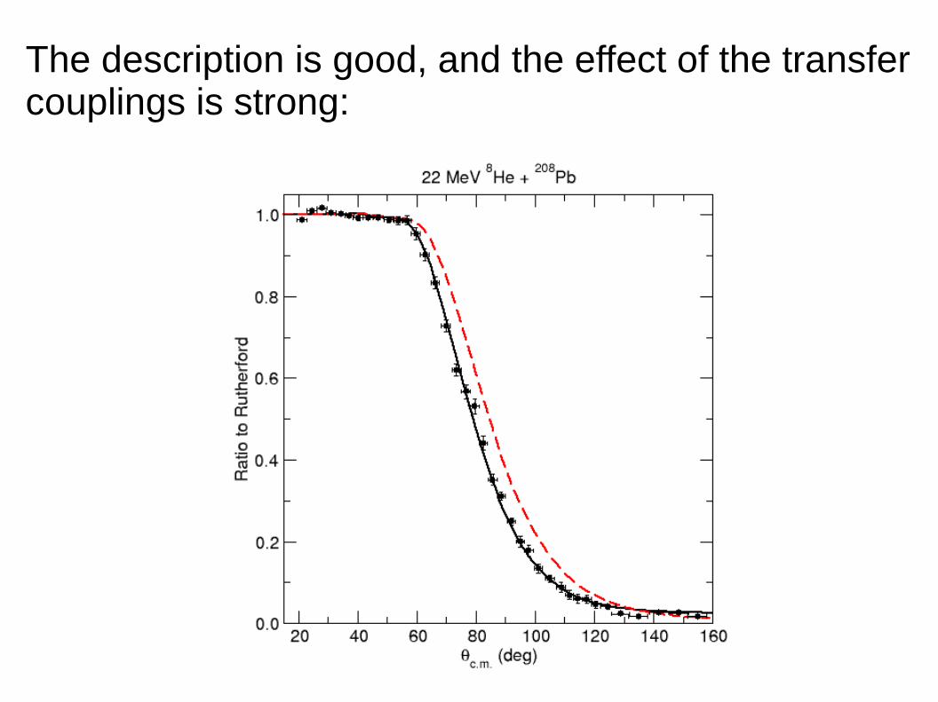
The description is good, and the effect of the transfercouplings is strong:

In fact, the 1n-stripping in this case accounts forabout 365 mb out of a total reaction cross sectionof 1517 mb, so about 24 %.

Thus it seems reasonable that the coupling effecton the elastic scattering is large (however, it is notalways so, and a large cross section does notguarantee a large coupling effect).

In fact, the 1n-stripping coupling accounts for about38 % of the total imaginary potential strength aswell as making a significant contribution to the realpart.

Thus we see that heavy ion induced transfer reactionscan also be interesting from the point of view of theirinfluence on the elastic scattering.

This is one of the major motivations for the study ofheavy ion reactions in general – their coupling effectson elastic scattering can be important and are oftenquite sensitive probes of the properties of thecolliding nuclei.

We have finally come to the end of this series oflectures on direct reactions and their analysis. Ihope that I have given a flavour of the interest andmotivation for such studies.

I have not touched on the interesting area of breakup reactions and their analysis, mainly through lack of time.

There are some other details of reaction analysistechniques that I have not mentioned, but you should now have enough knowledge to understanda direct reaction paper and assess it critically.