Direct solution of Navier–Stokes equations by radial basis functions

Available online at www.sciencedirect.com

Applied Mathematical Modelling 32 (2008) 1848–1858

www.elsevier.com/locate/apm

Direct solution of Navier–Stokes equationsby radial basis functions

G. Demirkaya a, C. Wafo Soh b, O.J. Ilegbusi a,*

a Department of Mechanical, Materials, and Aerospace Engineering, University of Central Florida,

4000 Central Florida Blvd., Orlando, FL 32816, USAb Department of Mathematics, College of Science, Engineering and Technology, Jackson State University,

P.O. Box 17619, Jackson, MS 39217, USA

Received 1 June 2006; received in revised form 1 May 2007; accepted 4 June 2007Available online 23 June 2007

Abstract

The pressure–velocity formulation of the Navier–Stokes (N–S) equation is solved using the radial basis functions (RBF)collocation method. The non-linear collocated equations are solved using the Levenberg–Marquardt method. The primarynovelty of this approach is that the N–S equation is solved directly, instead of using an iterative algorithm for the primitivevariables. Two flow situations are considered: Couette flow with and without pressure gradient, and 2D laminar flow in aduct with and without flow obstruction. The approach is validated by comparing the Couette flow results with the analyt-ical solution and the 2D results with those obtained using the well-validated CFD-ACETM commercial package.� 2007 Published by Elsevier Inc.

Keywords: Meshless method; Radial basis functions; Navier–Stokes equations

1. Introduction

Several computational methods have been applied to solve the Navier–Stokes equations, prominent amongwhich are the finite difference method (FDM), the finite element method (FEM) and the finite volume method(FVM). Although these methods have been successfully applied to many engineering situations, their accuracydepends critically on mesh quality. Specifically, appropriate mesh generation is typically a major difficulty incomputational fluid dynamics (CFD). If the geometry of the problem is complex, mesh generation, modifica-tion and re-meshing become difficult and time-consuming. Thus, numerical simulations and solution proce-dures using these traditional methods are often hampered by slow mesh generation.

Meshless methods have generated considerable interest recently due to the need to overcome the high costof mesh generation associated with human labor [1–12]. Mesh-free schemes avoid grid generation and thedomain of interest is discretized by a set of scattered points among which there is no pre-defined connectivity.

0307-904X/$ - see front matter � 2007 Published by Elsevier Inc.

doi:10.1016/j.apm.2007.06.019

* Corresponding author. Tel.: +1 407 823 1157; fax: +1 407 823 0208.E-mail address: [email protected] (O.J. Ilegbusi).

mailto:[email protected]

G. Demirkaya et al. / Applied Mathematical Modelling 32 (2008) 1848–1858 1849

In addition, geometry discretization is updated by simply adding or deleting points in the domain of interest.Previous meshless methods typically solve NS equations by using iterative schemes to solve the pressure-cor-rection equation. However, our approach in this paper differs from these methods in that, instead of using theprimitive variables (u, v, and p) in the iterative algorithm, we use a least-square method, which is inherentlyiterative, to find the unknown coefficients. The N–S and the boundary condition equations together constitutea system of non-linear equations, which are solved directly.

A number of meshless methods have been proposed. These methods include the smoothed particle hydro-dynamics method (SPH) [1], the diffuse element method (DEM) [2], the element-free Galerkin method(EFGM) [3], the reproducing kernel particle method (RKPM) [4], the partition of unity method (PUM) [5],the hp-clouds method (HPCM) [6], the finite point method (FPM) [7], the meshless local Petrov–Galerkinmethod (MLPGM) [8], the moving-particle semi-implicit method (MPSM) [9] and the general finite differencemethod (GFDM) [10]. Recently, a new meshless method was proposed based on the so-called radial basisfunctions (RBF) [11–17]. Kansa [11] introduced the direct collocation method using RBFs. To date, thismethod appears to be one of the most promising kernel approximation techniques because it produces a highlyefficient interpolation scheme, and can deal with unorganized data. In addition, it generally has better accu-racy on unorganized grids than the typical FDM based methods. RBF-based methods are also easier to imple-ment than traditional numerical schemes like FEM, FDM, and FVM.

Despite these advantages, the RFB-based methods are continuously being refined. Since the pioneeringwork of Kansa [11,12], several papers [13–24] have been dedicated to the improvement of RBF approachto PDEs. In a typical RBF iterative scheme, the equation under investigation is linearized about the previousiterate and a system of linear equations is solved at each iteration. As a rule, the matrix associated with thislinear system is very large, densely populated and ill-conditioned. Therefore, it is not surprising that severalsuggested RBF algorithms address these issues. Accuracy and stability are other important issues to considerwhen employing RBF. However, it should be pointed out that accuracy and stability of the solution dependstrongly on the type of RBF employed.

Relatively few studies have applied the meshless methods to solve convection-dominated flows. The finitepoint method [7] is one such method in which a non-element interpolation scheme with the weighted leastsquares (WLS) is used to solve the convection–diffusion problems. However, the presence of the convectionterm causes serious numerical difficulties, appearing in the form of ‘‘wiggles’’ (oscillatory solutions), whenthe convection term is dominant. Onate et al. [7] used the upwinding scheme with the FPM for the first deriv-ative to handle this problem. There is a significant drawback of the FPM as it is not easy to define the criticaldistance, which is important to stabilize the method and obtain good accuracy. In addition to this, the methodis based on point collocation, and is very sensitive to the choice of collocation points.

The meshless local Petrov–Galerkin (MLPG) method, have been developed in Zhu and Atluri [8], for solv-ing linear and non-linear boundary problems. Remarkable successes of the MLPG method have been reportedin solving the convection–diffusion problems, Navier–Stokes flows [25]. The MLPG method needs to intro-duce upwinding in order solve the convection–diffusion problems. MLPG works well for low Peclet numberflows, but is not good for high Peclet number flows. Atluri and Lin [25] indicated that the numerical integra-tion plays an important role in the convergence of numerical solutions of meshless methods, unfortunately, thenodal shape functions from meshless interpolations, such as Moving Least Squares, are highly complex in nat-ure. This feature makes an accurate numerical integration of the weak form highly difficult, especially in theconventional Galerkin type methods.

Meshless methods still require a considerable improvement, before they are equal to the convenience of thetraditional FDM, FVM, FEM, and BEM in computational fluid engineering area. However, in order to takefull advantage of the considerable potential of the meshless method, we have decided to implement the radialbasis function collocation method directly on N–S equations. In this paper, we present a novel approach foraccurate and stable solution of the Navier–Stokes equations using RBF. Specifically, instead of employing theclassical iterative approach to the solution of the RBF-collocated equations, we collocate the fully non-linearNavier–Stokes equation and solve the resulting non-linear system directly using the Levenberg–Marquardtmethod. This approach seems to produce accurate and stable results compared to the conventional iterativemethods. It is here applied to the classical Couette flow between two parallel plates with and without pressuregradient, and flow through a channel with and without an obstruction. The predicted Couette flow results

1850 G. Demirkaya et al. / Applied Mathematical Modelling 32 (2008) 1848–1858

mirror the analytical solutions, while the 2D results compare favorably with those obtained using the well-val-idated CFD-ACETM commercial package.

In order to examine the utility of this technique we have organized this paper into five sections of which thisintroduction is the first. In Section 2, we formulate and describe the numerical method used. Computationaldetails of the two classical flows under consideration are given in Section 3. The results are presented and com-pared with those of the commercial software CFD-ACE in Section 4. The last concluding Section 5 summa-rizes the major findings of the study.

2. Formulation

2.1. Systems considered

Two types of geometry are considered as shown in Fig. 1. Fig. 1a shows the Couette flow between parallelplates, Fig. 1b shows a 2D flow between two flat plates and finally, Fig. 1c shows a 2D flow between two flatplates with obstacle placed at the center of the bottom plate.

The meshless method requires a complete set of boundary conditions in order to obtain a solution. In thisstudy, the no-slip condition is imposed on all walls, implying upper wall velocity equal to U1, and zero veloc-ity on the lower wall for the Couette flow, and zero velocity on the walls for the 2D channel flow. The inflowvelocity for the 2D channel flow is specified with a mean velocity U1. The x-component of velocity is assumedto be equal to U1 at the inlet, the y-component of velocity is assumed to be zero, and the pressure is a ref-erence gage value of zero. The outlet is located sufficiently far from the inlet (L = 10H) to ensure fully-devel-oped flow in the channel. At the outlet, we assume that the flow exits with straight streamlines, the gradients ofall variables are zero in the flow direction and the continuity equation is satisfied. The wall and outlet pressureboundary equations are obtained by taking the scalar product of the momentum equation with the outwardnormal to the boundary. These boundary conditions are summarized in Table 1.

Fig. 1. Systems considered.

Table 1Boundary conditions

Velocity Pressure

Couette flow

Cwall u* = 1 v* = 0 @ y* = 1u* = 0 u* = 0 @ y* = 0

Channel flow

Cwall u* = 0 v* = 0 � op�

oy� þ 1Re

o2v�ox�2þ o2v�

oy�2

� �¼ 0 ðfor ny 6¼ 0 and nx ¼ 0Þ

� op�

ox� þ 1Re

o2u�ox�2 þ

o2u�oy�2

� �¼ 0 ðfor nx 6¼ 0 and ny ¼ 0Þ

Cinlet u* = 1 v* = 0 p* = 0Coutlet

ou�ox� þ ov�

oy� ¼ 0 ov�ox� ¼ 0 � op�

ox� þ 1Re

o2u�ox�2 þ

o2u�oy�2

� �� u� ou�

ox� þ v� ou�oy�

� �¼ 0


2.2. Governing equation

In this section, the new RBF method is described. It is then used to predict the velocity and pressure dis-tribution in a two-dimensional channel flow. The flow is assumed to be steady, viscous and incompressible.The Navier–Stokes equations for the flow in Cartesian coordinates are

ou�

ox�þ ov�

oy�¼ 0; ð1Þ

u�ou�

ox�þ v�

ou�

oy�¼ � op�

ox�þ 1

Reo

2u�

ox�2þ o

2u�

oy�2

� �; ð2Þ

u�ov�

ox�þ v�

ov�

oy�¼ � op�

oy�þ 1

Reo2v�

ox�2þ o2v�

oy�2

� �ð3Þ

in which all variables are non-dimensionalized, u* and v* represent the velocity components in the Cartesiancoordinate directions x* and y*, respectively, p* is the pressure, and Re is the Reynolds number (qU1D/l1)where D is the characteristic length of the domain, and q1 and U1 are the reference density and mean veloc-ity, respectively. The Cartesian coordinates x* and y* are non-dimensionalized with respect to D, u* and v* arenon-dimensionalized with respect to U1, and finally, p* is non-dimensionalized with respect to the dynamicpressure q1U 2

1.

2.3. Novelty of present approach

2.3.1. Solution method

The traditional pressure-correction methods are widely used to solve N–S equations. An example of thisapproach is the SIMPLE algorithm [26]. This method integrates the Navier–Stokes equations in time at eachtime-step by first solving the momentum equations using an approximate pressure field to yield an intermedi-ate velocity field that will not, in general, satisfy continuity. A Poisson equation is then solved with the diver-gence of the intermediate velocity as a source term to provide a pressure correction, which is then used tocorrect the intermediate velocity field, providing a divergence free velocity. The pressure is updated and inte-gration then proceeds to check the convergence. If the solution is converged the results are finalized. If not, theiterative process continues from the momentum equation with the new pressure and velocity field.

Kassab and Divo [21] combined the pressure-correction method with the radial basis collocation method tosolve heat diffusion–advection problems. Their approach, which is similar to the SIMPLE algorithm, is sum-marized as follows: The solution algorithm starts with an initial velocity field, which satisfies continuity, thenthe velocity field is introduced in the N–S equations, and the time derivatives are approximated using back-ward differencing, transforming the N–S to the Helmholtz Poisson equation set for estimating the velocityfield. Once the Helmholtz Poisson problem is solved subject to appropriate boundary conditions, the velocityfield is updated and forced to satisfy continuity. An equation to update the pressure field is obtained by takingthe divergence of the momentum equation and applying the continuity equation. The Poisson equation for thepressure field can be solved by imposing a proper and complete set of boundary conditions.


Our approach is distinct from the above in that, instead of using the primitive variables (u, v, and p) in theiterative algorithm, we use a least-square method, which is inherently iterative, to find the RBF expansioncoefficients. The N–S and the boundary condition equations together constitute a system of non-linear equa-tions, which are to be solved. These non-linear equations are then solved by one of the least-square methods,Levenberg–Marquardt. At the end we obtain the solutions of the velocity and pressure field directly. This pro-cedure is described in more detail below.

2.3.2. Radial basis function (RBF)

Consider the problem of finding a function whose values are known at a finite number of locations N. Wemay solve this problem by assuming that the unknown function is a linear combination of a complete set of N

functions. The coefficients of the linear combination are obtained by solving a linear system resulting from forc-ing the linear combination to take the given values at the N locations. In the RBF approach the complete set ofN functions are translated radial functions. Specifically, the approximation of a function f(x), using RBF is

f ðxÞ ffiXN

j¼1

ajWðkx� xjkÞ; ð4Þ

where k k is the Euclidian norm, N is the number of total collocation points, aj’s are the unknown coefficientsto be determined and W is the radial basis function. The interpolation coefficients a1,a2, . . . ,aN are determinedby solving the linear system of equations:

f ðxiÞ ffiXN

j¼1

ajWðrijÞ; i ¼ 1; . . . ;N ; ð5Þffiffiffiffiffiffiffiffiffiffiffiffiffiffiffiffiffiffiffiq

where rij ¼ ðxi � xjÞ2. The system of Eq. (5) can be written as

Wð0Þ Wðr12Þ Wðr13Þ � � � Wðr1N ÞWðr21Þ Wð0Þ Wðr23Þ � � � Wðr2N Þ

..

. ... ..

. ...

WðrN1Þ WðrN2Þ WðrN3Þ � � � WðrNN Þ

0BBBB@

1CCCCA

|fflfflfflfflfflfflfflfflfflfflfflfflfflfflfflfflfflfflfflfflfflfflfflfflfflfflfflfflfflfflfflfflfflfflfflfflfflfflfflfflffl{zfflfflfflfflfflfflfflfflfflfflfflfflfflfflfflfflfflfflfflfflfflfflfflfflfflfflfflfflfflfflfflfflfflfflfflfflfflfflfflfflffl}A

a1

a2

..

.

aN

0BBBB@

1CCCCA

|fflfflfflffl{zfflfflfflffl}a

¼

f1

f2

..

.

fN

0BBBB@

1CCCCA

|fflfflfflffl{zfflfflfflffl}fi

ð6Þ

or equivalently

Aa ¼ fi () a ¼ A�1fi; ð7Þ
where fi = f(xi).
The linear system of equations (7) can be solved numerically using techniques such as Gauss elimination.The coefficients a are back-substituted into Eq. (5) to obtain an approximation of f(x).

Common choices of W are

(a) Multi-quadratics (MQs): WðrÞ ¼ffiffiffiffiffiffiffiffiffiffiffiffiffiffir2 þ c2p

; c > 0.(b) Thin-plate splines (TPS): W(r) = r2n log(r), n is an integer.(c) Gaussians: WðrÞ ¼ e�cr2

; c > 0.(d) Inverse MQs: WðrÞ ¼ 1ffiffiffiffiffiffiffiffi

r2þc2p ; c > 0.

The shape parameter c defined in the MQs and Gaussian basis functions has an important role in theapproximation of the meshless methods. Although analyses are available for the shape parameter [27], thereis no mathematical theory on choosing its optimal value. We would like to eliminate this problem at this stagefor our proposed approach. We will use TPS RBF in this study since it does not require a shape parameter andits solution is not dependent on this parameter. Navier–Stokes equations is of second order, and we want toimprove and extend this method to 3D problems in the future, so we must use a higher order TPS [28,29] andthe integer n will be chosen as 2.


2.4. Expansion of the Navier–Stokes and boundary conditions by RBF

The velocity and pressure terms are globally expanded by collocation of all the points on the boundary anddomain as

ui ¼XNBþNI

a¼1

aiaWðk~r �~rakÞ i ¼ 1; 2 ðu� ¼ u1 and v� ¼ u2Þ; ð8Þ

p� ¼XNBþNI

a¼1

a0aWðk~r �~rakÞ; ð9Þ

where NB is the total number of boundary points enclosed in the domain, NI is the total internal points in thedomain, ai are the expansion coefficients and W is the radial basis expansion function.

The Navier–Stokes and boundary condition equations together constitute a system of non-linear equations,which are to be solved. The expanded velocity and pressure terms and their first and second derivatives aredirectly inserted into the equations. The boundary condition equations are collocated at the boundary points(i = 1..NB) and the continuity and momentum equations are collocated at the interior domain points(i = NB + 1. . .NB + NI). Then a non-linear system of equations for the unknown expansion coefficient a isformed as

F ðaÞ ¼ 0: ð10Þ
This non-linear system can be solved by the least-square optimization techniques such as the Levenberg–Mar-quardt method [30–32]. The Levenberg–Marquardt algorithm is an iterative technique that locates the mini-mum of a multivariate function that is expressed as the sum of squares of non-linear real-valued functions. Ithas become a standard technique for non-linear least-squares problems. The reader is referred to the literature[30–32] for further details of this method.
3. Computational details

The distribution of points in the domain for the flow situations considered is shown in Fig. 2. Fig. 2a rep-resents Couette flow between two channels, Fig. 2b represents flow through a 2D straight channel and Fig. 2cinvolves flow through a 2D channel with an obstruction on the lower wall. The obstruction is located mid-waybetween the inlet and the outlet. The non-dimensional length of the channel is 10, and the height is 1 in allcases. Fig. 2 shows that for Couette flow, a total of 42 (21 · 2) collocation points are used on the boundaryand 63 (21 · 3) collocation points are used in the interior for RBF expansion. For channel flow withoutobstruction, we used a total of 40 (15 · 2 + 10) collocation points on the boundary and 75 (5 · 15) collocationpoints in the interior. A total of 46 (21 + 15 + 10) collocation points are used on the boundary and 66 collo-cation points in the interior channel with obstruction.

This paper presents solutions at Re = 100. This case was chosen after systematic analysis of a number ofexamples over a wide range of Re. The Couette flow results are compared with the analytical solutions withand without pressure gradient while the 2D channel flow predictions are compared with those obtained usingthe finite volume method (FVM) approach embodied in the CFD–ACE computational package. In order to per-form error analysis, the relative percent error (e) is calculated for each node, and then the arithmetic mean (l)and the standard deviation (r) of the relative error are calculated for each case, using the following expressions:

e ¼ 100� X RBF � X CFD–ACE

X CFD–ACE

� �; ð11Þ

l ¼ 1

N

XN

i¼1

ei; ð12Þ

r ¼

ffiffiffiffiffiffiffiffiffiffiffiffiffiffiffiffiffiffiffiffiffiffiffiffiffiffiffiffiffiffi1

N

XN

i¼1

ðei � lÞ2vuut ð13Þ

in which X is any generic variable (velocity, pressure, stream function).

Fig. 2. Node distribution for Couette flow and 2D Channel flow considered.

Table 2A comparison of RBF CPU time with commercial CFD–ACE finite difference

Flow type Boundarynodes

Interiornodes

Totalnodes

CPU time (s) CFD–ACE (s)

Couette flow between 2 channels 42 63 105 35 NA (results compared with analysis)Channel flow with no obstruction 40 75 115 300 200Channel flow with obstruction 46 66 112 325 275


Our objective in the paper was to first demonstrate the feasibility of the direct solution approach usingRBF, which no one has attempted. Once the feasibility has been established in both 2D and 3D cases, we willset about optimization of the technique and code. However, in order to give an idea of the computational cost,we have summarized the CPU in Table 2 the computational costs of the three test cases compared with appli-cation of a commercial code. Specifically, it provides the CPU times required for the computations to be pre-sented in the following section, compared with the results obtained with the CFD–ACE commercial software.As expected, the CPU time for the meshless method depends on the number of nodes employed, as well as theLevenberg–Marquardt convergence criteria. However, a comparison of the results (following section) indi-cates that the node numbers indicated in Table 2 provide sufficiently accurate results. Considering that thereis still be room for optimization of the RBF code in the future, the computational costs as indicated in Tablecould be considered comparable to the commercial codes.

4. Results

4.1. Couette flow

The following three cases are investigated using RBF: (i) flow without pressure gradient; (ii) favorable(negative) pressure gradient; and (iii) adverse (positive) pressure gradient. The non-dimensional pressure


gradients considered in the streamwise x-direction for positive and negative cases are 0.05 and �0.05,respectively.

4.1.1. Zero pressure gradientThe predicted velocity vector for Couette flow with zero pressure gradient is presented in Fig. 3a while the

corresponding analytical solution is presented in Fig. 3b. The profile obtained with RBF compares favorablywith the exact analytical result. The arithmetic mean of the predicted relative error between the two sets ofresults is �0.00626%, and its standard deviation is 0.1558%, values which can be considered negligible.

4.1.2. Positive pressure gradient

The predicted velocity vectors with positive pressure gradient for RBF and analytical analysis are shown inFig. 4a and b, respectively. The RBF results are again quite close to the analytical results, with mean relativeerror between the two sets of results of 0.146% and standard deviation of 3.23%.

4.1.3. Negative pressure gradient

The predicted velocity vectors for negative pressure gradient case for RBF and analytical analysis areshown in Fig. 5a and b, respectively. The two sets of results are similar, with a mean relative error of0.17% and standard deviation of 0.69%, respectively between them.

Fig. 3. Predicted velocity vectors for Couette flow with zero pressure gradient for RBF (a) and exact analytical solution (b).

Fig. 4. Predicted velocity vectors for Couette flow with positive pressure gradient for RBF (a) and exact analytical solution (b).

Fig. 5. Predicted velocity vectors for Couette flow with negative pressure gradient for RBF (a) and exact analytical solution (b).


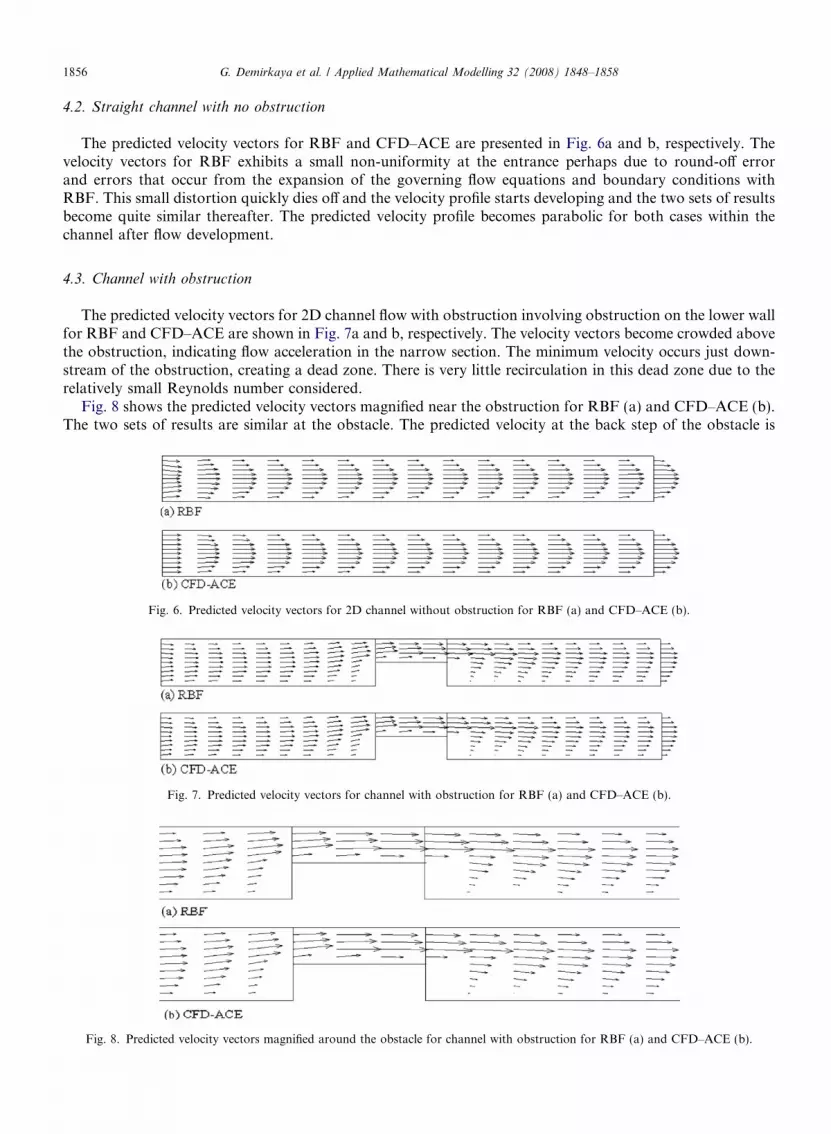
4.2. Straight channel with no obstruction

The predicted velocity vectors for RBF and CFD–ACE are presented in Fig. 6a and b, respectively. Thevelocity vectors for RBF exhibits a small non-uniformity at the entrance perhaps due to round-off errorand errors that occur from the expansion of the governing flow equations and boundary conditions withRBF. This small distortion quickly dies off and the velocity profile starts developing and the two sets of resultsbecome quite similar thereafter. The predicted velocity profile becomes parabolic for both cases within thechannel after flow development.

4.3. Channel with obstruction

The predicted velocity vectors for 2D channel flow with obstruction involving obstruction on the lower wallfor RBF and CFD–ACE are shown in Fig. 7a and b, respectively. The velocity vectors become crowded abovethe obstruction, indicating flow acceleration in the narrow section. The minimum velocity occurs just down-stream of the obstruction, creating a dead zone. There is very little recirculation in this dead zone due to therelatively small Reynolds number considered.

Fig. 8 shows the predicted velocity vectors magnified near the obstruction for RBF (a) and CFD–ACE (b).The two sets of results are similar at the obstacle. The predicted velocity at the back step of the obstacle is

Fig. 6. Predicted velocity vectors for 2D channel without obstruction for RBF (a) and CFD–ACE (b).

Fig. 7. Predicted velocity vectors for channel with obstruction for RBF (a) and CFD–ACE (b).

Fig. 8. Predicted velocity vectors magnified around the obstacle for channel with obstruction for RBF (a) and CFD–ACE (b).

Fig. 9. Predicted wall shear stress distribution along the lower wall for channel flow with obstruction.


small but negative in the x-direction, indicating a dead zone with a small recirculation. Subsequently the flowstarts to develop and recover to its original profile along the channel. The predicted recirculation length isapproximately 1.2H, extending from x� ¼ x

H ¼ 6 to x� ¼ xH ¼ 7:2.

The predicted shear stress distributions along the lower wall for channel flow with the obstacle are pre-sented in Fig. 9 for both RBF and CFD–ACE models. The two sets of results are generally in good agreement.The wall shear stress decreases from the channel entrance to the obstruction as the flow develops and thevelocity gradient decreases. Then it increases near the obstruction as the velocity gradient near the wallincreases. The stress continues to increase on the upstream part of the obstruction due to the favorable pres-sure gradient, reaching a peak at the center of the obstruction. Then it drops to its lowest value within therecirculation zone downstream of the obstruction. Subsequently the wall shear stress increases slowly as theflow recovers towards the outlet. The maximum relative error between the CFD–ACE and RBF shear stressresults is 1.719%, with a maximum standard deviation of 3.06%.

5. Conclusions

In this study, we have developed a novel method based on RBF for direction solution of the Navier–Stokesequations. We validated the proposed method by studying two classical flow situations, namely, the Couetteflow with and without pressure gradient, and 2D channel flows with and without obstruction. The predictedresults are then compared with the analytical solution for Couette flow and results obtained with and a well-validated commercial code for the channel flow.

Solution convergence was a major issue with RBF calculation. Convergence is significantly influenced bythe placement of the nodes. If node distribution is regular, the RBF method converges very quickly. As thenumber of points increases, the size of the Jacobian matrix used in the Levenberg–Marquardt methodemployed increases and slows down the solution algorithm. In extreme situations, the matrix may becomeill-conditioned.

The RBF method is well suited to problems involving complex geometry as it does not require the construc-tion of an elaborate grid typical of the traditional CFD methods. Despite the drawback of difficult conver-gence, the RBF approach proposed here has the potential to solve problems involving complex geometrycoupled with tools of parallel computing and some conditioning techniques.

This study has shown that the new method can compete with the traditional methods as far as accuracy isconcerned. Node distribution plays a crucial role in the accuracy of the RBF method. In addition, errors dueto the calculated derivatives evaluated directly from the RBF expansion can be significant if not carefully han-dled. Other techniques like weighted finite difference approximation may therefore be useful for such deriva-tives. The RBF method proposed here will be improved and applied to unsteady and higher-dimensionalproblems in a follow-up study.


Acknowledgements

The authors would like to acknowledge useful discussions with Dr. Alain. J. Kassab and Dr. EduardoDivo, both of the University of Central Florida.

References

[1] L.B. Lucy, A numerical approach to the testing of the fission hypothesis, Astron. J. 8 (1977) 1013–1024.[2] B. Nayroles, G. Touzot, P. Villon, Generalizing the finite element method: diffuse approximation and diffuse elements, Comput.

Mech. 10 (1992) 307–318.[3] T. Belytschko, Y.Y. Lu, L. Gu, Element-free Galerkin methods, Int. J. Numer. Methods Eng. 37 (1994) 229–256.[4] W. Liu, S. Jun, Y. Zhang, Reproducing kernel particle methods, Int. J. Numer. Methods Fluids 20 (1995) 1081–1106.[5] I. Babuska, J. Melenk, The partition of unity method, Int. J. Numer. Methods Eng. 40 (1997) 727–758.[6] C.A. Duarte, J.T. Oden, Hp clouds—a meshless method to solve boundary-value problems, TICAM Report 95-05.[7] E. Onate, S. Idelsohn, O.C. Zienkiewicz, R.L. Taylor, A finite point method in computational mechanics. Application to convective

transport and fluid flow, Int. J. Numer. Methods Eng. 39 (1996) 3839–3866.[8] S.N. Atluri, T. Zhu, New meshless local Petrov–Galerkin (MLPG) approach in computational mechanics, Comput. Mech. 22 (2)

(1998) 117–127.[9] S. Koshizuka, Y. Oka, Moving-particle semi-implicit method for fragmentation of incompressible fluid, Nucl. Sci. Eng. 123 (1996)

421–434.[10] T. Liszka, An interpolation method for an irregular net of nodes, Int. J. Numer. Methods Eng. 20 (1984) 1599–1612.[11] E.J. Kansa, Multiquadrics—A scattered data approximation scheme with applications to computational fluiddynamics—I. Surface

approximations and partial derivative estimates, Comput. Math. Appl. 19 (6–8) (1990) 127–145.[12] E.J. Kansa, Multiquadrics—A scattered data approximation scheme with applications to computational fluiddynamics—-II.

Solutions to parabolic, hyperbolic, and elliptic partial differential equations, Comput. Math. Appl. 19 (6–8) (1990) 147–161.[13] G.E. Fasshauer, Solving partial differential equations by collocation with radial basis functions, in: A.L. Mehaute, C. Rabut, L.L.

Schumaker (Eds.), Surface Fitting and Multiresolution Methods, 1997, pp. 131–138.[14] B. Jumarhon, S. Amini, K. Chen, The Hermite collocation method using radial basis functions, Eng. Anal. Bound. Elem. 24 (2000)

607–611.[15] T.A. Driscoll, B. Forberg, Interpolation in the limit of increasingly flat radial basis functions, Comput. Math. Appl. 43 (2002) 413–

422.[16] W. Chen, M. Tanaka, A. meshless, integration-free, and boundary-only RBF technique, Comput. Math. Appl. 43 (2002) 379–391.[17] C. Shu, H. Ding, K.S. Yeo, Local radial basis function-based differential quadrature method and its application to solve two-

dimensional incompressible Navier–Stokes equations, Comput. Methods Appl. Mech. Eng. 192 (2003) 941–954.[18] H. Takami, H.B. Keller, Steady two-dimensional viscous flow of an incompressible fluid past a circular cylinder, Phys. Fluids 12

(Suppl. II) (1969) 2–51.[19] Z. Wu, Solving PDE with radial basis function and the error estimation, in: Adv. Comput. Math., Lecture Notes on Pure and Applied

Mathematics, 1998, 202.[20] S.M. Wong, Y.C. Hon, T.S. Li, A meshless multi-layer model for a coastal system by radial basis functions, Comput. Math. Appl. 43

(3–4) (2002) 585–605.[21] E. Divo, A.J. Kassab, A meshless method for conjugate heat transfer problems, Eng. Anal. Boun. Elem. 29 (2005) 136–149.[22] T. Fujisawa, S. Ito, M. Inaba, G. Yagawa, Node-based parallel computing of three-dimensional incompressible flows using the free

mesh method, Eng. Anal. Boun. Elem. 28 (2004) 425–441.[23] I. Boztosun, A. Chara, M. Zerroukat, K. Djidjeli, Thin-plate spline radial basis function scheme for advection–diffusion problems,

Electron. J. Bound. Elem. BETEQ 2001 (2) (2002) 267–282.[24] J. Li, Y.C. Hon, C.S. Chen, Numerical comparisons of two meshless methods using radial basis functions, Comput. Methods Appl.

Mech. Eng. 194 (2005) 2001–2017.[25] H. Lin, S.N. Atluri, The meshless local Petrov–Galerkin (MLPG) method for solving incompressible Navier–Stokes equations,

CMES—Comput. Model. Eng. Sci. 2 (2) (2001) 117–142.[26] S.V. Patankar, Numerical Heat Transfer and Fluid Flow, Hemisphere Publishing Corporation, New York, 1980, ISBN 0-07-048740-

5.[27] A.H.-D. Cheng, M.A. Golberg, E.J. Kansa, G. Zammito, Exponential convergence and H-c multiquadric collocation method for

partial differential equations, Numer. Methods Partial Differen. Equat. 19 (5) (2003) 571–594.[28] M.D. Buhmann, Radial Basis Functions, Cambridge University Press, 2003.[29] M. Griebel, M.A. Schweitzer, Meshfree Methods for Partial Differential Equations, Springer, 2003.[30] K. Madsen, H.B. Nielsen, J. Sondergaard: Robust subroutines for non-linear optimization, Imm, Dtu, Report IMM-REP-2002-02.[31] K. Madsen, A combined Gauss–Newton and quasi-Newton method for non-linear least squares, Institute for Numerical Analysis,

DTU, Report NI-88-10.[32] K. Levenberg, A method for the solution of certain problems in least squares, Quart. Appl. Math. 2 (1944) 164–168.

Documents

Direct solution of Navier–Stokes equations by radial basis functions