Embed Size (px)
Citation preview
Univers
ity of
Cap
e Tow
n
Full Mueller Imaging
Direction Dependent Corrections in Polarimetric Radio Imaging
Preshanth Jagannathan

Univers
ity of
Cap
e Tow
n
The copyright of this thesis vests in the author. No quotation from it or information derived from it is to be published without full acknowledgement of the source. The thesis is to be used for private study or non-commercial research purposes only.
Published by the University of Cape Town (UCT) in terms of the non-exclusive license granted to UCT by the author.

Licensed under the Creative Commons Attribution-NonCommercial 3.0 Unported License(the “License”). You may not use this file except in compliance with the License. You mayobtain a copy of the License at http://creativecommons.org/licenses/by-nc/3.0.Unless required by applicable law or agreed to in writing, software distributed under theLicense is distributed on an “AS IS” BASIS, WITHOUT WARRANTIES OR CONDITIONS OF
ANY KIND, either express or implied. See the License for the specific language governingpermissions and limitations under the License.
Dec 2017

Acknowledgements
This thesis is a result of a four-year journey that has taken me across three continents. Itwould not have been possible but for the support of my supervisors, family and colleagues.At this juncture, I would like to thank a few of them that have been indispensable to myjourney. I would like to thank Russ Taylor who has been patient and supportive of me. Hehas found time to answer my questions and provide guidance no matter the continent ortimezone either of us was in. Without him, this thesis and I might not have made it to thisjuncture.
Another instrumental figure in this journey is Sanjay Bhatnagar, my co-supervisor. Hehas been kind enough to take me under his wing and guided me through the worlds ofradio interferometry and algorithm developments. My interactions with Sanjay have beenilluminating to me both scientifically and personally and I am very fortunate to have afriend and mentor in him. He has also spent the better part of the last year poring overthese pages to make it more user friendly for the reader. Sanjay, thank you for everything,I am excited about getting back to Socorro and start working with you again.
Many people at NRAO have contributed towards this thesis undertaking, I wouldespecially like to thank my collaborators Urvashi Rau, and Walter Brisken for taking thetime to answer my myriad questions no matter how trivial. Kumar Golap and Urvashi Rauhave been an encyclopedia of CASA knowledge and without them, my work would haveprogressed at a much much slower pace. I would like to thank Vivek Dhawan, Rick Perleyand Peter Napier for the many holography and primary beam related discussions whichhave helped in improving my understanding of the instrument. My thanks to Steve Myersfor playing devil’s advocate throughout, and for raising my morale with his witticisms.Thanks, Huib Intema for the many hours of discussions on interferometry and imaging andfor the opportunity to work and learn with him on the TGSS ADR project. I would alsolike to thank Erik Bryer and James Robnett for their invaluable help with deploying mycode on HPC architecture.
My time in NRAO Socorro as a Reber fellow has been rewarding both professionally

and personally. I would like to thank NRAO for supporting me financially for the last threeyears through the Reber fellowship program. I am especially thankful for the coffee groupin Room 300, for the much-needed sustenance in terms of caffeine and company.
My parents and my sister have been a source of consistent support and encouragement,and I want to thank them for it. Ramya, you have been the source of my strength andsanity these past years of my PhD. As my wife and best friend you have helped shore upmy moral when I needed it the most and for that I thank you.
All software written for this project has made use of open-source development packagesand code within CASA. I would also like to acknowledge the Python software developmentcommunity, in particular, NumPy, SciPy, Matplotlib and, Seaborn packages which havebeen used extensively in this thesis.

Contents
1 Introduction . . . . . . . . . . . . . . . . . . . . . . . . . . . . . . . . . . . . . . . . . . . . . . . . . 7
1.1 Motivation 71.1.1 Goals . . . . . . . . . . . . . . . . . . . . . . . . . . . . . . . . . . . . . . . . . . . . . . . . . . . . . . . . 11
1.2 Overview of the thesis 111.3 Radio Polarimetry 121.3.1 Polarization ellipse & the Poincaré sphere . . . . . . . . . . . . . . . . . . . . . . . . . 121.3.2 Stokes Parameters . . . . . . . . . . . . . . . . . . . . . . . . . . . . . . . . . . . . . . . . . . . . . . 151.3.3 Jones Calculus . . . . . . . . . . . . . . . . . . . . . . . . . . . . . . . . . . . . . . . . . . . . . . . . 161.3.4 Mueller Calculus . . . . . . . . . . . . . . . . . . . . . . . . . . . . . . . . . . . . . . . . . . . . . . . 16
2 Radio Interferometry . . . . . . . . . . . . . . . . . . . . . . . . . . . . . . . . . . . . . . 192.0.1 Spatial Coherence Function . . . . . . . . . . . . . . . . . . . . . . . . . . . . . . . . . . . . . 19
2.1 Matrix formulation of the measurement equation 212.2 Calibration 232.3 Imaging 242.3.1 Imaging through Optimization . . . . . . . . . . . . . . . . . . . . . . . . . . . . . . . . . . . 252.3.2 Gridding and De-gridding . . . . . . . . . . . . . . . . . . . . . . . . . . . . . . . . . . . . . . . 27
2.4 Direction Dependent Gains and Projection Algorithms 292.4.1 W-Projection . . . . . . . . . . . . . . . . . . . . . . . . . . . . . . . . . . . . . . . . . . . . . . . . . . 292.4.2 Antenna Primary Beam . . . . . . . . . . . . . . . . . . . . . . . . . . . . . . . . . . . . . . . . . 30
3 Direction Dependent Effects . . . . . . . . . . . . . . . . . . . . . . . . . . . . . 33
3.1 Introduction 333.2 Primary Beam as a Direction Dependent Effect 33

3.3 Simulations 373.3.1 An Off-Axis Point Source as viewed by a single interferometric baseline 383.3.2 Polarization Fidelity and Observing Interval . . . . . . . . . . . . . . . . . . . . . . . . 393.3.3 Effect on Rotation Measure Synthesis . . . . . . . . . . . . . . . . . . . . . . . . . . . . . 403.3.4 Effects of Primary Beam Squash . . . . . . . . . . . . . . . . . . . . . . . . . . . . . . . . . . 433.4 Conclusion 44
4 Antenna Aperture Illumination . . . . . . . . . . . . . . . . . . . . . . . . . . . 474.1 A-Solver 484.1.1 Physical Modeling of the AIP . . . . . . . . . . . . . . . . . . . . . . . . . . . . . . . . . . . . 484.2 Measuring the PB through holography 504.2.1 Holography . . . . . . . . . . . . . . . . . . . . . . . . . . . . . . . . . . . . . . . . . . . . . . . . . . . 514.3 Optimizing the model through holography 514.3.1 Apparent Central Blockage . . . . . . . . . . . . . . . . . . . . . . . . . . . . . . . . . . . . . 534.3.2 Feed Illumination Taper . . . . . . . . . . . . . . . . . . . . . . . . . . . . . . . . . . . . . . . . . 544.3.3 Pointing Offset . . . . . . . . . . . . . . . . . . . . . . . . . . . . . . . . . . . . . . . . . . . . . . . . . 554.3.4 Antenna AIP and Imaging . . . . . . . . . . . . . . . . . . . . . . . . . . . . . . . . . . . . . . . 554.3.5 Imaging Simulations . . . . . . . . . . . . . . . . . . . . . . . . . . . . . . . . . . . . . . . . . . . . 594.4 Conclusions 60
5 Full Mueller A-Projection . . . . . . . . . . . . . . . . . . . . . . . . . . . . . . . . . 635.1 A-Projection Algorithm 635.1.1 The Full Polarization Antenna AIP . . . . . . . . . . . . . . . . . . . . . . . . . . . . . . . . . 645.2 Simulations with point sources 675.2.1 Simulated Deep Field . . . . . . . . . . . . . . . . . . . . . . . . . . . . . . . . . . . . . . . . . . . 685.3 Full Mueller Imaging of Supernova Remnant G55.7+3.4 725.3.1 Calibration . . . . . . . . . . . . . . . . . . . . . . . . . . . . . . . . . . . . . . . . . . . . . . . . . . . . 725.3.2 Full Mueller Imaging . . . . . . . . . . . . . . . . . . . . . . . . . . . . . . . . . . . . . . . . . . . . 725.3.3 Rotation Measure Synthesis . . . . . . . . . . . . . . . . . . . . . . . . . . . . . . . . . . . . . . 735.4 Conclusions 74
6 Algorithms & Computation . . . . . . . . . . . . . . . . . . . . . . . . . . . . . . . 796.1 Parallel Optimization & Solving for parameterized AIP 796.2 Full Mueller - AW Projection Implementation 80
7 Conclusion . . . . . . . . . . . . . . . . . . . . . . . . . . . . . . . . . . . . . . . . . . . . . . . . 837.1 Full Mueller A-Projection & Polarimetric Imaging 837.2 Future Work 85
Appendix . . . . . . . . . . . . . . . . . . . . . . . . . . . . . . . . . . . . . . . . . . . . . . . . . . 87
Bibliography . . . . . . . . . . . . . . . . . . . . . . . . . . . . . . . . . . . . . . . . . . . . . . . 89Books 89Articles 89

1. Introduction
1.1 Motivation“A very large part of space-time must be investigated, if reliable results are to
be obtained.”—Alan Turing
Magnetic fields pervade the universe, spanning a multitude of scales from the dipolarfield on Earth, to the largest gravitationally bound structures such as galaxy clusters [1].The magnetic fields play a vital role in the evolution of these astronomical systems. Inaddition to the multitude of scales, magnetic fields are present in different astronomicalsystems of varying strengths. The strongest observed astronomical magnetic fields are inneutron stars with a field strength of ≈ 1015 G [2], far higher than any man-made fieldstill date. In stark contrast magnetic fields in the interstellar medium while ubiquitousare only a few µG in field strength. Many fundamental processes in astrophysics havemagnetism at their heart, be it cosmic ray particle acceleration, star formation, or thelaunch of radio galaxy jets, pulsars, etc. One key fundamental process that allows us todetect and characterize cosmic magnetic fields with radio astronomy is the polarization ofsynchrotron radiation.
Synchrotron radiation is intrinsically polarized broadband continuum radiation emittedby relativistic charged particles accelerated by the presence of magnetic fields. The emis-sivity of the synchrotron radiation is tied to the magnetic field strength B and the spectralindex α (defined such that the flux density S ∝ ν−α ) such that ε ∝ B1+α . Radio continuumobservations measuring the total intensity and accurate spectral index measurements area direct probe of the source magnetic field. While total intensity measurements providethe magnetic field strength, measurements of the fractional polarization in the emissionare related to the degree of order in the source magnetic field, over the volume contained
8 Chapter 1. Introduction
in the angular resolution of the observation. Polarization angle (also known as the elec-tric vector polarization angle) is another measure that can be derived from the linearlypolarized emission. The polarization angle of the source is related to the direction of thesource magnetic field. The observed polarization angle is affected by Faraday rotation, aphenomenon by which intervening plasmas between the source and the telescope rotatethe plane of polarization. Faraday depth φ of the source as defined by [3] is,
φ = 812∫ 0
LneB||dl (1.1)
where L is the path length along the line of sight in kpc, ne is the electron density ofthe plasma in cm−3 and B|| is the magnetic field component parallel to the line of sight.Faraday rotation can be thought of in terms of refractive optics such that the magnetizedplasma has a different refractive index for each of the orthogonal components of theincident polarizations of the radio waves. This would result in the slowing down of oneof the polarization inputs with respect to the other, which manifests as a rotation in theobserved polarization angle of the radio waves (refer Chen [4] for a detailed derivation).
As shown in Eq.1.1, the Faraday rotation of the incident angle of polarization due to anintervening magnetized plasma is a function of a) the electron density of the interveningplasma and b) the strength and direction of the magnetic field component along the line ofsight. These factors collectively define the strength of the RM signal that can be observed.In cases where both the Faraday depth along the line of sight and the electron densityof the intervening plasma are available the magnetic field structure along the sight canbe gleaned. In practice, because φ is an integrated quantity, it is difficult to measure theelectron density of various intervening plasmas along the line of sight which means it is notpossible to dissociate various components of Faraday depth φ in terms of plasma magneticfields at a known distance between the source and the telescope. In the limiting case of Lbeing the distance of the source the Faraday depth reduces to the source rotation measure(RM) given by,
Ω = Ω0 +RMλ2 (1.2)
where Ω is the measured angle of polarization, Ω0 is the true angle of polarization of thesource and λ is the wavelength of observation. Brentjens and de Bruyn [5] introduced RMsynthesis a technique for the reconstruction of linear polarization as a function of Faradaydepth from the measured complex polarized intensity as a function of λ 2 despite limitedcoverage in λ 2 domain (For a detailed overview of the technique and its implementationrefer Sec. 3.3.3.)
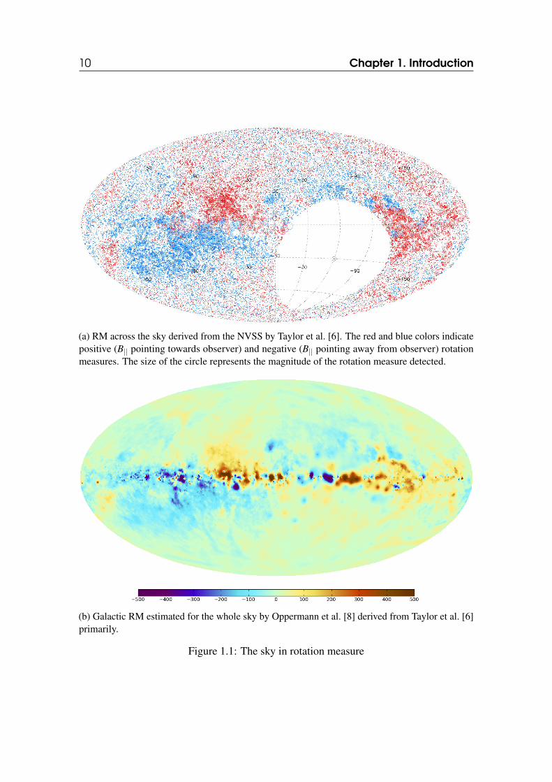
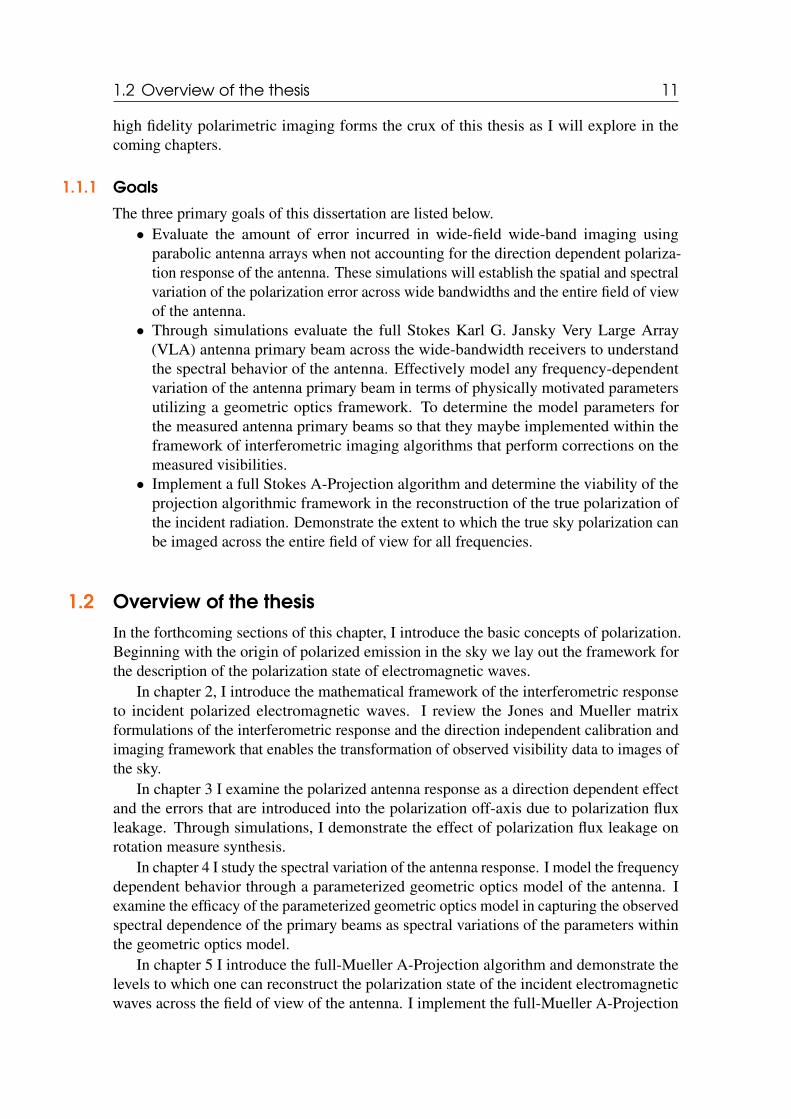
Large area spectro-polarimetric surveys have produced grids of RM values to back-ground sources allowing us to study the polarization and depolarization properties of radiosources and consequently their magnetic field properties and the RM signatures of theGalactic foregrounds. Taylor et al. [6] derived the largest catalog of polarized sourcesproducing an RM grid of sources from the NRAO VLA sky survey (NVSS) [7] shownin Fig. 1.1a. They obtained a catalog of 37543 polarized radio sources spanning over80% of the sky. An all-sky background of RM then allows us to study the interveningmagneto-ionic media in a statistical fashion as demonstrated by Oppermann et al. [8] inestimating the median galactic RM map, shown in Fig. 1.1b. Using the estimated mediangalactic RM Oppermann et al. [9] determined the extragalactic contribution arising from
1.1 Motivation 9
the magneto-ionic media outside our galaxy to a polarized source to be minimal, ≤ 7rad/m2. The background RM grid of sources has been used to probe the magnetic fieldstructure of intervening sources from coronal mass ejection of the sun (Kooi et al. [10]), tonebulae(Savage et al. [11]; Purcell et al. [12]; Costa et al. [13]), to our own Galactic Halo(Mao et al. [14]), to galaxies (Stil [15]), and clusters of galaxies (Lawler and Dennison[16]).
Magnetic fields in galaxies also manifest a variety of depolarization mechanisms(differential Faraday rotation, internal Faraday dispersion) (Sokoloff et al. [17]). Thesedepolarization mechanisms have been utilized to study the large scale magnetic fields ofnearby galaxies (Heald et al. [18];Stil et al. [19]). In the cases where the radio sourcedisplays significant depolarization in addition to polarized emission, it is essential tounderstand Π(λ 2), i.e. the fractional polarization (Π) as a function of λ 2 [20]. They showthat a source with two spatially unresolved RM components can produce an apparent linearbehavior of the polarization position angle as a function of λ 2 a degeneracy broken whenexamining the fractional polarization.
Beyond nearby galaxies, deep radio observations have enabled the study of polarizedemission and magnetic field evolution across cosmic time. Observations by Mesa et al.[21] and Taylor et al. [22] indicate an increase in fractional polarization with decreasingflux density for sources down to 500µJy in polarized intensity. This suggests a change ineither the magnetic field structure or the Faraday screen surrounding these objects, or theemergence of a different class of objects [21]. Deeper observations down to the 10µJyby Hales et al. [23] and Rudnick and Owen [24] observe no trend of increasing fractionalpolarization with flux density. Since the primary limitation of deep fields is the samplesize of the sources used in determining the nature of the ensemble a next generation surveythat is both deep and wide is required to truly determine the nature of the faintly polarizedpopulation.
The next generation of radio polarimetric surveys are a part of a new era of wide-band, wide-area, full Stokes continuum surveys on parabolic antenna interferometer arrays.These surveys will collect data over very large instantaneous bandwidths in the GHzfrequency regime. From past surveys [25], it is known that at the minimum a quarter ofthe observed polarized sources will display complex behavior in Faraday depth (Law et al.[25];O’Sullivan et al. [26]). To accurately reconstruct the true nature of these polarizedsources either through RM synthesis [5] or model fitting [26], it is essential to producehigh-fidelity, high dynamic range images in all polarization states of the incoming radiationover the full field-of-view of the array antennas. While interferometric arrays record data inall polarizations the recorded data has inter-mixing of polarization states. Reconstructionof pure polarization states of the incoming electromagnetic waves to a high fidelity is animaging requirement for all next-generation instruments.
Imaging algorithms to date have focused on achieving high fidelity and high dynamicrange imaging primarily only in total power. In the absence of high fidelity reconstructionof polarization states across the entire field of view, polarimetry is restricted to sources veryclose to the antenna pointing centers. While this is a time consuming means of studyingindividual sources of interest, it limits our ability to survey and map the polarizationstate of the entire sky efficiently. It is therefore vital to extend the existing algorithmicframework to account for wide-field polarization effects during radio interferometric imagereconstruction. The process of extending the existing algorithmic framework to achieve
10 Chapter 1. Introduction
(a) RM across the sky derived from the NVSS by Taylor et al. [6]. The red and blue colors indicatepositive (B|| pointing towards observer) and negative (B|| pointing away from observer) rotationmeasures. The size of the circle represents the magnitude of the rotation measure detected.
(b) Galactic RM estimated for the whole sky by Oppermann et al. [8] derived from Taylor et al. [6]primarily.
Figure 1.1: The sky in rotation measure
1.2 Overview of the thesis 11
high fidelity polarimetric imaging forms the crux of this thesis as I will explore in thecoming chapters.
1.1.1 Goals
The three primary goals of this dissertation are listed below.• Evaluate the amount of error incurred in wide-field wide-band imaging using
parabolic antenna arrays when not accounting for the direction dependent polariza-tion response of the antenna. These simulations will establish the spatial and spectralvariation of the polarization error across wide bandwidths and the entire field of viewof the antenna.• Through simulations evaluate the full Stokes Karl G. Jansky Very Large Array
(VLA) antenna primary beam across the wide-bandwidth receivers to understandthe spectral behavior of the antenna. Effectively model any frequency-dependentvariation of the antenna primary beam in terms of physically motivated parametersutilizing a geometric optics framework. To determine the model parameters forthe measured antenna primary beams so that they maybe implemented within theframework of interferometric imaging algorithms that perform corrections on themeasured visibilities.• Implement a full Stokes A-Projection algorithm and determine the viability of the
projection algorithmic framework in the reconstruction of the true polarization ofthe incident radiation. Demonstrate the extent to which the true sky polarization canbe imaged across the entire field of view for all frequencies.
1.2 Overview of the thesisIn the forthcoming sections of this chapter, I introduce the basic concepts of polarization.Beginning with the origin of polarized emission in the sky we lay out the framework forthe description of the polarization state of electromagnetic waves.
In chapter 2, I introduce the mathematical framework of the interferometric responseto incident polarized electromagnetic waves. I review the Jones and Mueller matrixformulations of the interferometric response and the direction independent calibration andimaging framework that enables the transformation of observed visibility data to images ofthe sky.
In chapter 3 I examine the polarized antenna response as a direction dependent effectand the errors that are introduced into the polarization off-axis due to polarization fluxleakage. Through simulations, I demonstrate the effect of polarization flux leakage onrotation measure synthesis.
In chapter 4 I study the spectral variation of the antenna response. I model the frequencydependent behavior through a parameterized geometric optics model of the antenna. Iexamine the efficacy of the parameterized geometric optics model in capturing the observedspectral dependence of the primary beams as spectral variations of the parameters withinthe geometric optics model.
In chapter 5 I introduce the full-Mueller A-Projection algorithm and demonstrate thelevels to which one can reconstruct the polarization state of the incident electromagneticwaves across the field of view of the antenna. I implement the full-Mueller A-Projection
12 Chapter 1. Introduction
algorithm within the Common Astronomy Software Application framework and show itsperformance on measured data from the VLA.
In chapter 6 I examine the performance of the implementation of the full-MuellerA-Projection algorithm, its limitations and the scope of improvements that will be exploredin the future.
1.3 Radio PolarimetryOne of the primary mechanisms of radio emission is synchrotron radiation. Synchrotronradiation is the emission of electromagnetic waves by ultra-relativistic electrons that areaccelerated by a magnetic field into gyrations. Synchrotron radiation is observed from ourgalaxy, supernova remnants and external radio galaxies, particularly at the centimeter andmeter wavelengths. It is the dominant source of cosmic radiation as low frequency
If we consider a charged particle of mass m0 and charge ze, moving at a relativisticvelocity~v, and Lorentz factor γ in a uniform magnetic field ~B, its equation of motion canbe written as,
γm0d~vdt
= ze(~v×~B). (1.3)
One can separate the components of the particle velocity into a parallel and perpendicularcomponent. With only the perpendicular component being altered by the magnetic field,causing the particle to undergo gyrations around the magnetic field lines. The parallelcomponent of the velocity couples to enable a helical motion in the most general case.This accelerated charged particle emits in along the direction of acceleration which isperpendicular to both the velocity vector v and the direction of the magnetic field B. If weconsider the case of the charged particle to be an electron we can determine its energy lossrate as,
−dEdt
=γ4e2
6πε0c3 a⊥ =e4B2
6πε0cm2e
v2
c2 γ2sin2
θ (1.4)
where me is the mass of the electron and ε0 is the emissivity of free space, a⊥ is theperpendicular acceleration vector. The energy loss rate −dE
dt in the ultra-relativistic limitv→ c is converted into synchrotron radiation that is emitted across a wide spectrumof frequencies as electromagnetic waves from high energy X-rays to radio waves. Theradiation that is emitted is highly polarized (for a detailed derivation of the polarized natureof the emitted radiation refer Pacholczyk [27]).
Since the incoming electromagnetic wave is the only vector observable there are streamsof astronomy dedicated to observing and analyzing the different aspects of the vector.The electromagnetic wave can be completely characterized by knowing the amplitude(photometry), frequency (spectroscopy), the direction of its poynting vector (imaging) andthe orientation of the electric and magnetic field vectors with respect to a reference frame(polarimetry).
1.3.1 Polarization ellipse & the Poincaré sphereSince Maxwell’s equations impose the condition that the direction of either field cannot bealong the direction of propagation we can determine the polarization state of the wave by
1.3 Radio Polarimetry 13
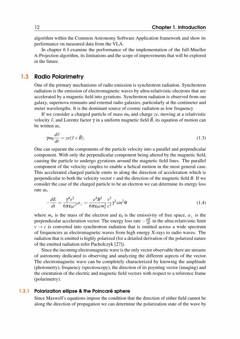
Figure 1.2: The polarization ellipse is shown in the xy plane. Where a and b are thesemi-major and semi-minor axes of the ellipse. ψ is the inclination of the semi-major axisof the ellipse with respect to the local x coordinate axis.
looking at either the electric or magnetic field vectors. In radio astronomy, only the voltagesinduced by the incident electric field on an antenna is measured and so the descriptionhenceforth will be focused on the electric field vector of an electromagnetic wave. Let usconsider a Cartesian coordinate system that is oriented such that the z-axis is pointed alongthe line of sight. Then the electric field vector is oscillating in the xz and yz planes whilepropagating towards us along the z-axis. The equation of electromagnetic waves can thenbe written as
~E = Exx+Eyy = E0xei(2πνt+δx)x+E0yei(2πνt+δy)y, (1.5)
where ~E is the electric field vector, E0x and E0y are the amplitudes of the electric fieldcomponents Ex and Ey along the x and y axes. x and y are the unit vectors along the x andy axes. δx and δy are the phases of the electric field components. The electric field vectoris moving helically in three dimensions whose projection on the xy plane corresponds tothe polarization ellipse. The ellipse equation can then be written as,
E2x
E2x0+
E2y
E2y0− 2ExEyη
Ex0Ey0= sin2(η), (1.6)
where η = δx−δy is the phase difference between electric field phases along the x andy axes. Some special cases of the polarization ellipse are of particular interest, Ex0 = Ey0and η = 0 is when the wave is perfectly linearly polarized. Similarly, when Ex0 = Ey0and η =±pi/2 we get a circularly polarized wave, when the phase is positive the electricfield vector rotates in a clockwise direction also known as right circular polarization(RCP) and when the phase is negative the electric field vector rotates in an anti-clockwisedirection known as the left circular polarization (LCP). A more compact representation of
14 Chapter 1. Introduction
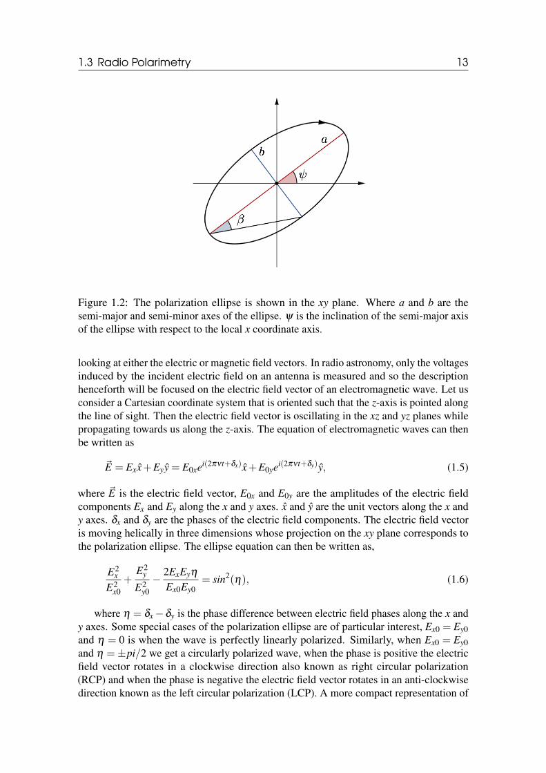
Figure 1.3: The Poincaré sphere of a polarization vector P(2ψ,2β ) is shown. The Cartesianaxes, S1, S2 and S3, form the Stokes parameter axes, as the projection of the P along eachof the axes gives rise to the polarized Stokes parameters.
the polarization state of the electric field vector can be had in the polar coordinates of thepolarization ellipse. In the polar form, the polarization ellipse is constrained only by theratio of the semi-major (a) and semi-minor axes (b) given by sin(2β ), and the inclinationangle of the electric field vector with respect to the x-axis of the coordinate frame tan(2ψ)as shown in Fig. 1.2.
tan(2ψ) =2Ex0Ey0cosη
E2x0−E2
y0(1.7)
sin(2β ) =2Ex0Ey0sinη
E2x0 +E2
y0(1.8)
Henri Poincaré demonstrated that any polarization state can then be represented on asphere utilizing the ellipticity parameter (2β ) as the longitude, the azimuth angle of thepolarization ellipse (2ψ) as the latitude, and the amplitude of the electric field vector givenby P = (E2
x0 +E2y0) as the radius of the sphere as shown in fig 1.3. The sphere provides a
compact representation of the different polarization states and consequently the differentbasis in which the electric field vector is represented. The states are defined as follows:• Linear Polarization : When 2β = 0, and 2ψ = 0, the electric field vector is horizon-
tally polarized. When2β = 0 and 2ψ = 180 the electric field vector is verticallypolarized.• Circular Polarization : When 2ψ = 90 for all β the vector is considered to be
circularly polarized.• Elliptical Polarization : All other states of polarization barring the special cases of
linear and circular polarization with arbitrary values of ψ and β constitute ellipticalpolarization.
In the Poincaré sphere the radius vector from the origin to the surface corresponds to the
1.3 Radio Polarimetry 15
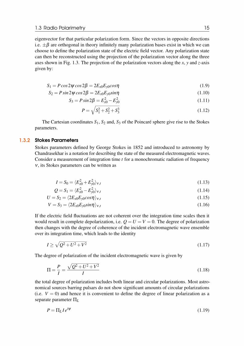
eigenvector for that particular polarization form. Since the vectors in opposite directionsi.e. ±β are orthogonal in theory infinitely many polarization bases exist in which we canchoose to define the polarization state of the electric field vector. Any polarization statecan then be reconstructed using the projection of the polarization vector along the threeaxes shown in Fig. 1.3. The projection of the polarization vectors along the x, y and z-axisgiven by:
S1 = P cos2ψ cos2β = 2Ex0Ey0cosη (1.9)S2 = P sin2ψ cos2β = 2Ex0Ey0sinη (1.10)
S3 = P sin2β = E2x0−E2
y0 (1.11)
P =√
S21 +S2
2 +S33 (1.12)
The Cartesian coordinates S1, S2 and, S3 of the Poincaré sphere give rise to the Stokesparameters.
1.3.2 Stokes ParametersStokes parameters defined by George Stokes in 1852 and introduced to astronomy byChandrasekhar is a notation for describing the state of the measured electromagnetic waves.Consider a measurement of integration time t for a monochromatic radiation of frequencyν , its Stokes parameters can be written as
I = S0 = 〈E2x0 +E2
y0〉ν ,t (1.13)
Q = S1 = 〈E2x0−E2
y0〉ν ,t (1.14)U = S2 = 〈2Ex0Ey0cosη〉ν ,t (1.15)V = S3 = 〈2Ex0Ey0sinη〉ν ,t (1.16)
If the electric field fluctuations are not coherent over the integration time scales then itwould result in complete depolarization, i.e. Q =U =V = 0. The degree of polarizationthen changes with the degree of coherence of the incident electromagnetic wave ensembleover its integration time, which leads to the identity
I ≥√
Q2 +U2 +V 2 (1.17)
The degree of polarization of the incident electromagnetic wave is given by
Π =PI=
√Q2 +U2 +V 2
I(1.18)
the total degree of polarization includes both linear and circular polarizations. Most astro-nomical sources barring pulsars do not show significant amounts of circular polarizations(i.e. V = 0) and hence it is convenient to define the degree of linear polarization as aseparate parameter ΠL
P = ΠL I eiψ (1.19)

16 Chapter 1. Introduction
where ΠL is the fractional linear polarization and ψ the electric vector polarization angle.ΠL and ψ are defined in terms of the observed Stokes parameters as,
ΠL =
√Q2 +U2
I(1.20)
ψ =12
tan−1(
UQ
)(1.21)
high fidelity measurement of the complex polarization vector P of the incident electromag-netic wave is one of the primary goals of radio polarimetry.
1.3.3 Jones CalculusWhile the Stokes parameters are convenient to describe the state of the ensemble ofmeasured electromagnetic waves, it is not a convenient form to describe the transformationsthat the incident electromagnetic waves have undergone. The Jones vector 〈E〉ν ,t is definedas
〈E〉ν ,t =(〈Ex0eiηx〉〈Ey0eiηy〉
)ν ,t
(1.22)
The Jones vector is defined by the amplitude and phase of the electric field vector in the xand y directions. Any transformation of the Jones vector can then be represented as a 2×2Jones matrix. The Jones matrices are then operators that describe the transformations ofthe Jones vector such as polarization mixing, birefringence etc. In subsequent chapters ofthis thesis we will revisit the role of the Jones matrix in radio interferometry
1.3.4 Mueller CalculusThe Mueller calculus is a means of manipulating the Stokes vectors themselves to representtransformations of the incident electromagnetic waves. Introduced by Hans Mueller in1943, it extended the Jones Calculus formalism to include the most general descriptionof an optical transformation of the incident electromagnetic wave. The measured Stokesvector ~S′ is the transformation of the emitted Stokes vector ~S by the 4×4 Mueller matrixM.
I′
Q′
U ′
V ′
=
M00 M01 M02 M03M10 M11 M12 M13M20 M21 M22 M23M30 M31 M32 M33
IQUV
(1.23)
The Mueller matrix is a transform matrix of the incident polarized electromagnetic wavesit does not retain phase information of incident electric field, unlike the Jones matrix whichworks directly on electric fields themselves. In the case of polarized electromagnetic wavesthe Jones matrices can be transformed into the Mueller matrix by means of the tensorproduct operation, M = J⊗J∗, where J∗ is the complex conjugate of the Jones matrix J. Itis also worthwhile noting that the basis of representation of the incident electromagneticwaves determines the basis of the Mueller matrix that is applied to it. Any orthogonalbasis of representation of the Stokes vectors such as circular (R,L, right and left circularly

1.3 Radio Polarimetry 17
polarized), or linear basis (X ,Y ) are equivalent to each other. For a more detailed overviewof the matrix transformation from one basis to another is can be found in the Appendix.
Armed with the Jones and Mueller calculi I will apply it in the context of the measure-ment equation of a radio interferometer, in the next chapter. I will also explore directionindependent calibration and the direction dependent nature of polarization leakage as itpertains to the antenna response function also called the antenna primary beam.

18 Chapter 1. Introduction
2. Radio Interferometry
In order to understand the Full-Mueller A-Projection algorithm, it is vital that we under-stand the modern formulation of the measurement equation. With that goal in mind, I willrevisit some fundamental concepts of interferometry and the framework upon which thesimulations and algorithms of the forthcoming chapters are built. The notation used in thischapter follows Hamaker et al. [28] and Rau et al. [29]. The derivation of spatial coherenceof an electric field follows chapter 1 of Taylor et al. [30].
2.0.1 Spatial Coherence Function
To image a source with an interferometer the source of interest must be an incoherentemitter, i.e the there is no spatial correlation in the emission from one region of the sourceto the other. If you consider a source that is a monochromatic emitter of electromagneticwaves and the emission is constant over time, we can write the emission from a direction~ras the vector ε(~r, t) = εν(~r)e−2πiνt , where εν(~r) is the complex amplitude of the electricfield vector. Consider the electric field of a quasi-monochromatic EM-wave originatingfrom the source at ~R and is incident on the detector location at~r. Under the assumptionsthat, the intervening space between the source and detector is empty we can relate thecomplex amplitude of the electric field at the detector Eν(~r) to the EM-wave of frequencyν originating at the source of strength εν(~r) through Huygen’s principle.
Eν(~r) =∫
εν(~R)e2πiν |~R−~r|/c
|~R−~r|dS (2.1)
where S is the projected shape of the source on the two-dimensional celestial sphere anddS is the elemental area of the projected source shape. The spatial coherence of the electricfields incident at two locations ~r1 and ~r2 on the detector originating from two locations ~R1
20 Chapter 2. Radio Interferometry
and ~R2 within the source S can be expressed as follows.
〈Eν(~r1)E∗ν(~r2)〉= 〈∫ ∫
εν(~R1)ε∗ν(~R2)
e2πiν |~R1−~r1|/c
|~R1−~r1|e2πiν |~R2−~r2|/c
|~R2−~r2|dS1dS2〉 (2.2)
If the source is an incoherent emitter 〈εν(~r1)ε∗ν(~r2)〉 = 〈|εν |2〉δ (~r1− ~r2) = 〈|εν(~R)|2〉,
where ~R1 = ~R2 = ~R. If the distance of the source vastly exceeds the size of detector then~R >> ~r1,~r2 then 1
|~R−~r1|, 1|~R−~r2|
→ 1|R| . Each source element dS can be written in terms of
the solid angle subtended on the celestial sphere by the source, as seen by the detector as|R|2dΩ. If s is the unit vector along ~R and we define Iν(s) = 〈|εν(s)|2〉 as the observedintensity of the source at the detector, Eq. 2.2 reduces to
〈Eν(~r1)E∗ν(~r2)〉=∫
Iν(s)e−2πiνs.|~r1−~r2|/cdΩ (2.3)
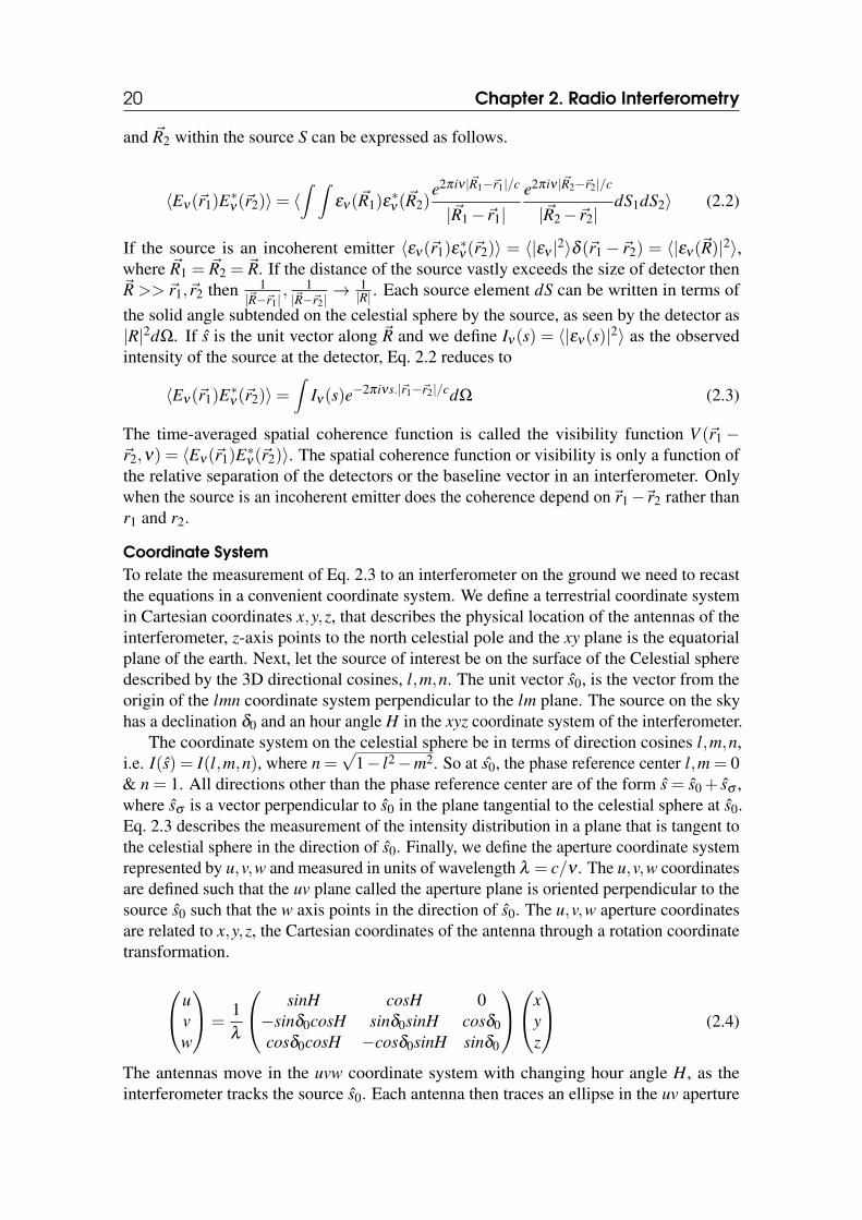
The time-averaged spatial coherence function is called the visibility function V (~r1−~r2,ν) = 〈Eν(~r1)E∗ν(~r2)〉. The spatial coherence function or visibility is only a function ofthe relative separation of the detectors or the baseline vector in an interferometer. Onlywhen the source is an incoherent emitter does the coherence depend on~r1−~r2 rather thanr1 and r2.
Coordinate SystemTo relate the measurement of Eq. 2.3 to an interferometer on the ground we need to recastthe equations in a convenient coordinate system. We define a terrestrial coordinate systemin Cartesian coordinates x,y,z, that describes the physical location of the antennas of theinterferometer, z-axis points to the north celestial pole and the xy plane is the equatorialplane of the earth. Next, let the source of interest be on the surface of the Celestial spheredescribed by the 3D directional cosines, l,m,n. The unit vector s0, is the vector from theorigin of the lmn coordinate system perpendicular to the lm plane. The source on the skyhas a declination δ0 and an hour angle H in the xyz coordinate system of the interferometer.
The coordinate system on the celestial sphere be in terms of direction cosines l,m,n,i.e. I(s) = I(l,m,n), where n =
√1− l2−m2. So at s0, the phase reference center l,m = 0
& n = 1. All directions other than the phase reference center are of the form s = s0 + sσ ,where sσ is a vector perpendicular to s0 in the plane tangential to the celestial sphere at s0.Eq. 2.3 describes the measurement of the intensity distribution in a plane that is tangent tothe celestial sphere in the direction of s0. Finally, we define the aperture coordinate systemrepresented by u,v,w and measured in units of wavelength λ = c/ν . The u,v,w coordinatesare defined such that the uv plane called the aperture plane is oriented perpendicular to thesource s0 such that the w axis points in the direction of s0. The u,v,w aperture coordinatesare related to x,y,z, the Cartesian coordinates of the antenna through a rotation coordinatetransformation.
uvw
=1λ
sinH cosH 0−sinδ0cosH sinδ0sinH cosδ0cosδ0cosH −cosδ0sinH sinδ0
xyz
(2.4)
The antennas move in the uvw coordinate system with changing hour angle H, as theinterferometer tracks the source s0. Each antenna then traces an ellipse in the uv aperture
2.1 Matrix formulation of the measurement equation 21
plane, this phenomenon is called the earth rotation aperture synthesis. A baseline vectorof two antennas given by the 3D vector~b(u,v,w) = ~r1−~r2. The non zero w value meanswe have to introduce a time delay τ =~bs0/ν = (w1−w2)/ν to ensure that the pair ofantennas are sampling the same wavefront in the direction s0. A point of note is that w is afunction of (δ ,H) and hence is a direction dependent effect. The delay τ corrects for onlythe direction of s0. Directions in the sky away from the phase center (s0) still possess a nonzero w− term that needs to be corrected during imaging. Finally, we have a finite numberof antennas sampling the aperture plane in uv denoted by S(u,v), the sampling function
S(u,v) = W(u,v)∑n
δ (u−un)δ (v− vn) (2.5)
where n is the index of baselines. The sampling is an instantaneous delta function inu,v of the 3D baseline vector. The instantaneous sampling changes with earth rotationand the cumulative sampling S(u,v), represents the spatial frequencies sampled by theinterferometer. We can then recast Eq. 2.3 in terms of coordinate system we have createdfor the aperture and the sky planes.
V obs(u,v,w) = S(u,v,w)∫ ∫
I(l,m,n)e−2πi(ul+vm+w(n−1))
ndldm (2.6)
where V obs(u,v,w) =V (u,v,w) ·S(u,v), is the visibilities sampled by the interferometerdiscretized per baseline. For a coplanar array (w = 0) or when imaging a small region ofthe sky such that l2 +m2 ' 1 resembles Eq. 2.6 reduces to
V obs(u,v)≈ S(u,v,w)∫ ∫
I(l,m)e−2πi(ul+vm)dldm (2.7)
An interferometer then measures the spatial frequencies corresponding to the Fouriertransform of the sky brightness distribution as measured by a pair of antennas. This isknown as the van Cittert-Zernike theorem (Thompson et al. [31]), or the measurementequation and is at the heart of interferometry. The image made using the data from all thebaselines is a convolution of the Fourier transform of the sampling function (FS ) and thesky brightness distribution (~Isky). The effects of the sampling function S are removed as apart of imaging as discussed in subsequent sections.
2.1 Matrix formulation of the measurement equationFor full Stokes imaging, we need to include the full polarization description of the emissionfrom the sky and the full polarization response of the interferometer. Consider a quasi-monochromatic electromagnetic wave emitted by a single point source in the sky, as itpropagates towards us the observer, given by ε . We can then write the measured voltageat the feed of antenna a in an interferometric baseline as, ~V = Ja ·~ε . In terms of theorthogonal feed basis p and q of the antenna a.
~V = Ja ·~ε = Ja
(epeq
)(2.8)
where Ja is the Jones matrix that contains all the linear transformation occurring affectingthe incident EM wave. The feed basis p,q can be replaced with any orthogonal basis such
22 Chapter 2. Radio Interferometry
as the linear X ,Y , or circular R,L basis, without any loss of generality. The transforma-tions that the signal might be subjected to along its propagation path can be completelycharacterized in terms of a 2× 2 Jones matrix under the assumptions that the interven-ing transformations are linear. The transformation falls under two categories, directionindependent (DI, such as receiver gains, leakages, etc) and direction dependent (DD gains,such as ionospheric delays, primary beam) We will revisit the effect of the Jones matriceson the signal in the discussion on calibration and imaging.
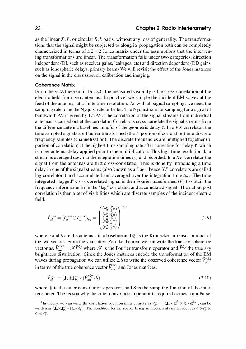
Coherence MatrixFrom the vCZ theorem in Eq. 2.6, the measured visibility is the cross-correlation of theelectric field from two antennas. In practice, we sample the incident EM waves at thefeed of the antennas at a finite time resolution. As with all signal sampling, we need thesampling rate to be the Nyquist rate or better. The Nyquist rate for sampling for a signal ofbandwidth ∆ν is given by 1/2∆ν . The correlation of the signal streams from individualantennas is carried out at the correlator. Correlators cross-correlate the signal streams fromthe difference antenna baselines mindful of the geometric delay τ . In a FX correlator, thetime sampled signals are Fourier transformed (the F portion of correlation) into discretefrequency samples (channelization). The discrete frequencies are multiplied together (Xportion of correlation) at the highest time sampling rate after correcting for delay τ , whichis a per antenna delay applied prior to the multiplication. This high time resolution datastream is averaged down to the integration times tint and recorded. In a XF correlator thesignal from the antennas are first cross-correlated. This is done by introducing a timedelay in one of the signal streams (also known as a "lag", hence XF correlators are calledlag correlators) and accumulated and averaged over the integration time tint . The timeintegrated "lagged" cross-correlated signal is then Fourier transformed (F) to obtain thefrequency information from the "lag" correlated and accumulated signal. The output postcorrelation is then a set of visibilities which are discrete samples of the incident electricfield.
~V obsab = 〈~εobs
a ⊗~εobsb 〉tint =
〈ep
aepb∗〉
〈epaeq
b∗〉〈eq
aepb∗〉
〈eqaeq
b∗〉
obs
(2.9)
where a and b are the antennas in a baseline and ⊗ is the Kronecker or tensor product ofthe two vectors. From the van Cittert-Zernike theorem we can write the true sky coherencevector as, ~V sky
ab = F~Isky where F is the Fourier transform operator and~Isky the true skybrightness distribution. Since the Jones matrices encode the transformation of the EMwaves during propagation we can utilize 2.8 to write the observed coherence vector ~V obs
abin terms of the true coherence vector ~V sky
ab and Jones matrices.
~V obsab = (Ja~J∗b)? (~V
skyab ·S) (2.10)
where ~ is the outer convolution operator1, and S is the sampling function of the inter-ferometer. The reason why the outer convolution operator is required comes from Parse-
1In theory, we can write the correlation equation in its entirety as ~V obsab = (Ja ? ε
skya ~J∗b ? ε
skyb ), can be
written as (Ja~J∗b)? (εa~ε∗b ). The condition for the source being an incoherent emitter reduces εa~ε∗b toεa⊗ ε∗b .
2.2 Calibration 23
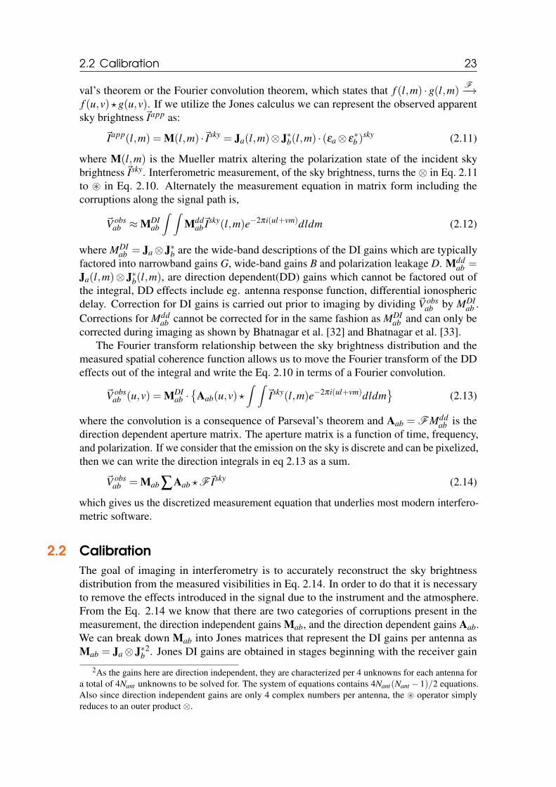
val’s theorem or the Fourier convolution theorem, which states that f (l,m) · g(l,m)F−→
f (u,v)?g(u,v). If we utilize the Jones calculus we can represent the observed apparentsky brightness~Iapp as:
~Iapp(l,m) = M(l,m) ·~Isky = Ja(l,m)⊗J∗b(l,m) · (εa⊗ ε∗b )
sky (2.11)
where M(l,m) is the Mueller matrix altering the polarization state of the incident skybrightness~Isky. Interferometric measurement, of the sky brightness, turns the ⊗ in Eq. 2.11to ~ in Eq. 2.10. Alternately the measurement equation in matrix form including thecorruptions along the signal path is,
~V obsab ≈MDI
ab
∫ ∫Mdd
ab~Isky(l,m)e−2πi(ul+vm)dldm (2.12)
where MDIab = Ja⊗J∗b are the wide-band descriptions of the DI gains which are typically
factored into narrowband gains G, wide-band gains B and polarization leakage D. Mddab =
Ja(l,m)⊗ J∗b(l,m), are direction dependent(DD) gains which cannot be factored out ofthe integral, DD effects include eg. antenna response function, differential ionosphericdelay. Correction for DI gains is carried out prior to imaging by dividing ~V obs
ab by MDIab .
Corrections for Mddab cannot be corrected for in the same fashion as MDI
ab and can only becorrected during imaging as shown by Bhatnagar et al. [32] and Bhatnagar et al. [33].
The Fourier transform relationship between the sky brightness distribution and themeasured spatial coherence function allows us to move the Fourier transform of the DDeffects out of the integral and write the Eq. 2.10 in terms of a Fourier convolution.
~V obsab (u,v) = MDI
ab ·
Aab(u,v)?∫ ∫
~Isky(l,m)e−2πi(ul+vm)dldm
(2.13)
where the convolution is a consequence of Parseval’s theorem and Aab = FMddab is the
direction dependent aperture matrix. The aperture matrix is a function of time, frequency,and polarization. If we consider that the emission on the sky is discrete and can be pixelized,then we can write the direction integrals in eq 2.13 as a sum.
~V obsab = Mab ∑Aab ?F~Isky (2.14)
which gives us the discretized measurement equation that underlies most modern interfero-metric software.
2.2 CalibrationThe goal of imaging in interferometry is to accurately reconstruct the sky brightnessdistribution from the measured visibilities in Eq. 2.14. In order to do that it is necessaryto remove the effects introduced in the signal due to the instrument and the atmosphere.From the Eq. 2.14 we know that there are two categories of corruptions present in themeasurement, the direction independent gains Mab, and the direction dependent gains Aab.We can break down Mab into Jones matrices that represent the DI gains per antenna asMab = Ja⊗J∗b
2. Jones DI gains are obtained in stages beginning with the receiver gain
2As the gains here are direction independent, they are characterized per 4 unknowns for each antenna fora total of 4Nant unknowns to be solved for. The system of equations contains 4Nant(Nant −1)/2 equations.Also since direction independent gains are only 4 complex numbers per antenna, the ~ operator simplyreduces to an outer product ⊗.
24 Chapter 2. Radio Interferometry
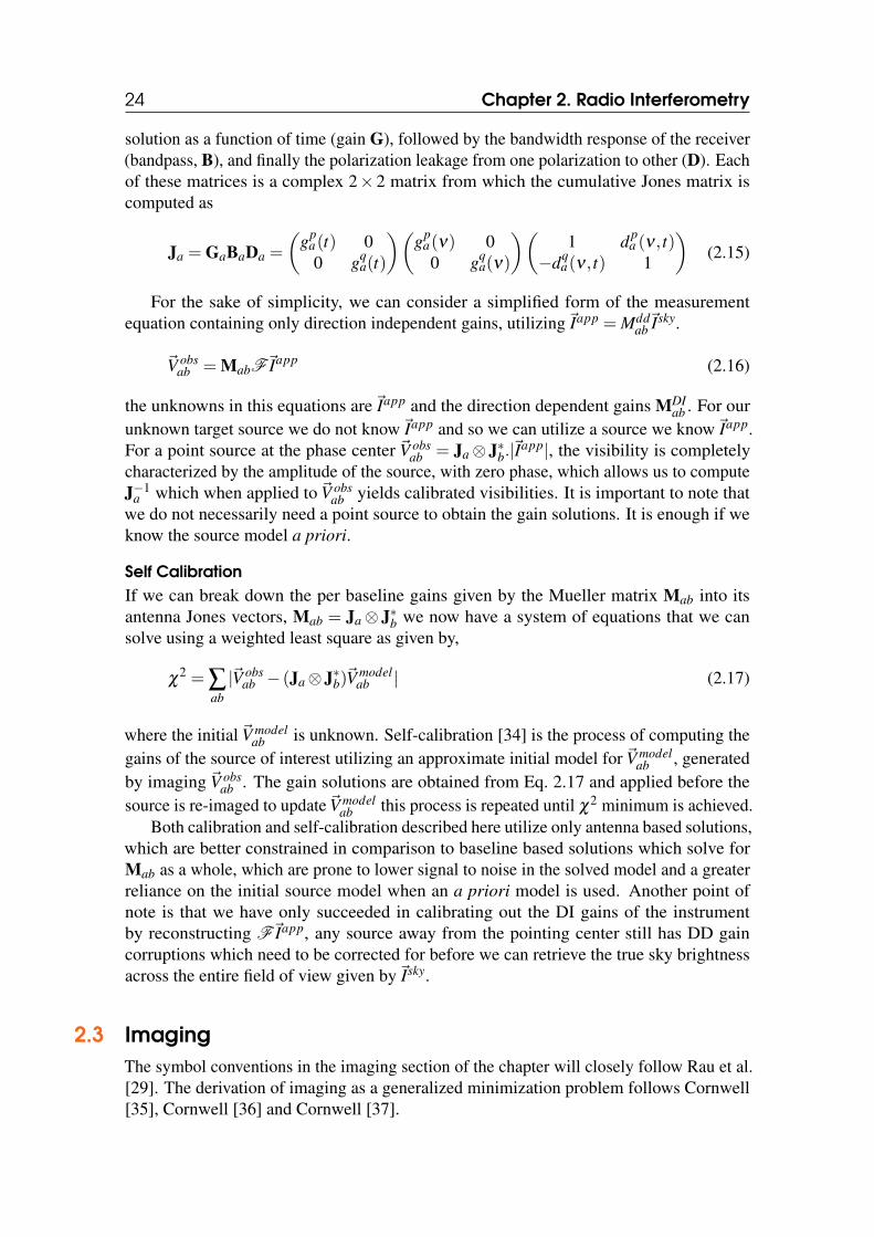
solution as a function of time (gain G), followed by the bandwidth response of the receiver(bandpass, B), and finally the polarization leakage from one polarization to other (D). Eachof these matrices is a complex 2× 2 matrix from which the cumulative Jones matrix iscomputed as
Ja = GaBaDa =
(gp
a(t) 00 gq
a(t)
)(gp
a(ν) 00 gq
a(ν)
)(1 dp
a (ν , t)−dq
a(ν , t) 1
)(2.15)
For the sake of simplicity, we can consider a simplified form of the measurementequation containing only direction independent gains, utilizing~Iapp = Mdd
ab~Isky.
~V obsab = MabF~Iapp (2.16)
the unknowns in this equations are~Iapp and the direction dependent gains MDIab . For our
unknown target source we do not know~Iapp and so we can utilize a source we know~Iapp.For a point source at the phase center ~V obs
ab = Ja⊗ J∗b.|~Iapp|, the visibility is completelycharacterized by the amplitude of the source, with zero phase, which allows us to computeJ−1
a which when applied to ~V obsab yields calibrated visibilities. It is important to note that
we do not necessarily need a point source to obtain the gain solutions. It is enough if weknow the source model a priori.
Self CalibrationIf we can break down the per baseline gains given by the Mueller matrix Mab into itsantenna Jones vectors, Mab = Ja⊗ J∗b we now have a system of equations that we cansolve using a weighted least square as given by,
χ2 = ∑
ab|~V obs
ab − (Ja⊗J∗b)~Vmodelab | (2.17)
where the initial ~V modelab is unknown. Self-calibration [34] is the process of computing the
gains of the source of interest utilizing an approximate initial model for ~V modelab , generated
by imaging ~V obsab . The gain solutions are obtained from Eq. 2.17 and applied before the
source is re-imaged to update~V modelab this process is repeated until χ2 minimum is achieved.
Both calibration and self-calibration described here utilize only antenna based solutions,which are better constrained in comparison to baseline based solutions which solve forMab as a whole, which are prone to lower signal to noise in the solved model and a greaterreliance on the initial source model when an a priori model is used. Another point ofnote is that we have only succeeded in calibrating out the DI gains of the instrumentby reconstructing F~Iapp, any source away from the pointing center still has DD gaincorruptions which need to be corrected for before we can retrieve the true sky brightnessacross the entire field of view given by~Isky.
2.3 ImagingThe symbol conventions in the imaging section of the chapter will closely follow Rau et al.[29]. The derivation of imaging as a generalized minimization problem follows Cornwell[35], Cornwell [36] and Cornwell [37].
2.3 Imaging 25
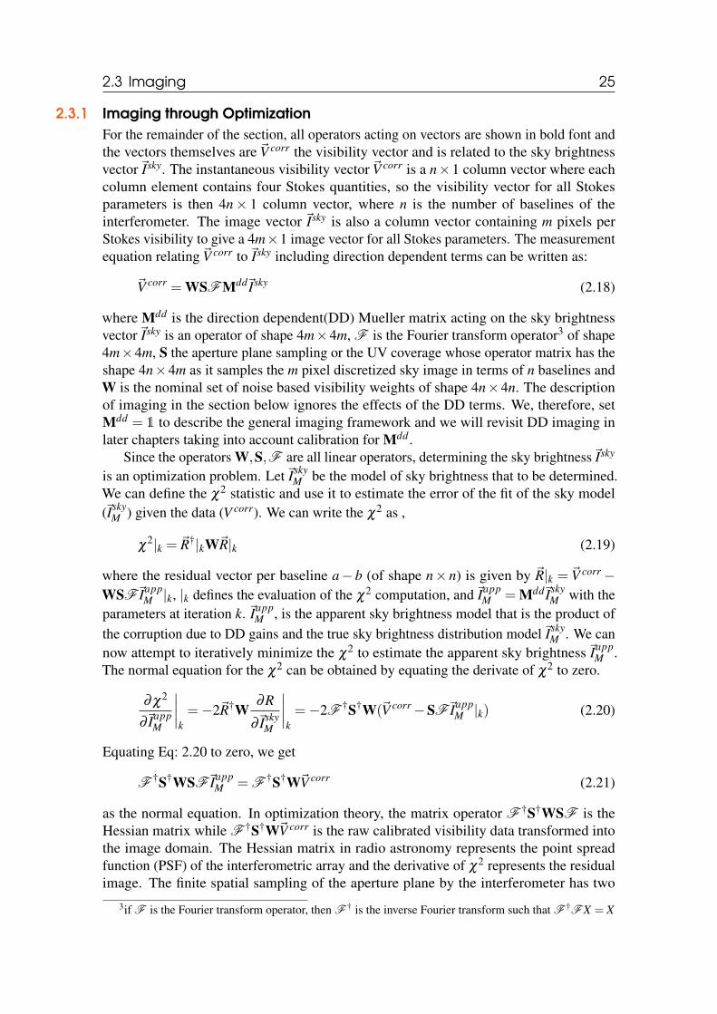
2.3.1 Imaging through OptimizationFor the remainder of the section, all operators acting on vectors are shown in bold font andthe vectors themselves are ~V corr the visibility vector and is related to the sky brightnessvector~Isky. The instantaneous visibility vector ~V corr is a n×1 column vector where eachcolumn element contains four Stokes quantities, so the visibility vector for all Stokesparameters is then 4n× 1 column vector, where n is the number of baselines of theinterferometer. The image vector ~Isky is also a column vector containing m pixels perStokes visibility to give a 4m×1 image vector for all Stokes parameters. The measurementequation relating ~V corr to~Isky including direction dependent terms can be written as:
~V corr = WSFMdd~Isky (2.18)
where Mdd is the direction dependent(DD) Mueller matrix acting on the sky brightnessvector~Isky is an operator of shape 4m×4m, F is the Fourier transform operator3 of shape4m×4m, S the aperture plane sampling or the UV coverage whose operator matrix has theshape 4n×4m as it samples the m pixel discretized sky image in terms of n baselines andW is the nominal set of noise based visibility weights of shape 4n×4n. The descriptionof imaging in the section below ignores the effects of the DD terms. We, therefore, setMdd = 1 to describe the general imaging framework and we will revisit DD imaging inlater chapters taking into account calibration for Mdd .
Since the operators W,S,F are all linear operators, determining the sky brightness~Isky
is an optimization problem. Let~IskyM be the model of sky brightness that to be determined.
We can define the χ2 statistic and use it to estimate the error of the fit of the sky model(~Isky
M ) given the data (V corr). We can write the χ2 as ,
χ2|k = ~R†|kW~R|k (2.19)
where the residual vector per baseline a− b (of shape n× n) is given by ~R|k = ~V corr−WSF~Iapp
M |k, |k defines the evaluation of the χ2 computation, and~IappM = Mdd~Isky
M with theparameters at iteration k. ~Iapp
M , is the apparent sky brightness model that is the product ofthe corruption due to DD gains and the true sky brightness distribution model~Isky
M . We cannow attempt to iteratively minimize the χ2 to estimate the apparent sky brightness~Iapp
M .The normal equation for the χ2 can be obtained by equating the derivate of χ2 to zero.
∂ χ2
∂~IappM
∣∣∣∣k=−2~R†W
∂R
∂~IskyM
∣∣∣∣k=−2F †S†W(~V corr−SF~Iapp
M |k) (2.20)
Equating Eq: 2.20 to zero, we get
F †S†WSF~IappM = F †S†W~V corr (2.21)
as the normal equation. In optimization theory, the matrix operator F †S†WSF is theHessian matrix while F †S†W~V corr is the raw calibrated visibility data transformed intothe image domain. The Hessian matrix in radio astronomy represents the point spreadfunction (PSF) of the interferometric array and the derivative of χ2 represents the residualimage. The finite spatial sampling of the aperture plane by the interferometer has two
3if F is the Fourier transform operator, then F † is the inverse Fourier transform such that F †FX = X
26 Chapter 2. Radio Interferometry
consequences for the equation, a) It renders the Hessian matrix singular and rules out asimple inversion of the matrix to solve the normal equation. b) It introduces an impulseresponse function or point spread function into the measurement.
~Ips f is the PSF or the response function in the direction of the image produced by apoint source on the sky in that direction. From Eq. 2.18 the PSF of the image can bederived by replacing~Iapp with a point source of unit source flux density placed at the phasecenter ~V corr
ab then becomes 1 and
~Ips f = F †S†W†1. (2.22)
The PSF shape is determined by the weighted UV coverage, and the width of the PSF andconsequently, maximum resolution of the interferometric array is θ = 1
Bmax, where Bmax is
the maximum baseline length in wavelengths. The finite sampling means~Ips f as shownin Eq. 2.22 has positive and negative side-lobes due to the missing spacings between theshortest and longest spatial frequencies, and a sharp cut-off beyond the largest sampledspatial frequencies of the interferometer.
Since the Hessian in Eq. 2.21 is not invertible we will have to solve the normal equationusing an iterative Newton-Raphson approach to obtain Iobs
M .1. Initialize any prior image model we might have as Isky
M , and in the absence of a prioriinformation an empty image model. The residual vector image is defined as
~Ires|k = F †S†W~R|k = F †S†W(~V corr−SF~IappM |k) (2.23)
For n = 0 and~IappM |k = 0, then~Idirty =~Ires|k=0, is the raw image, also called the dirty
image of the sky obtained by taking a Fourier transform of the calibrated visibilities.When ~Isky
M 6= 0 the computation of the model visibilities as, ~V mod = SF~IappM |k is
called the predict step or forward transform used to determine the residuals visibilityvector ~V res|k =~V corr−~V mod|k. Equivalently the computation of the residual image~Ires = F †SW~V res is called the reverse transform or the imaging step. The operationof updating the model image and computing the residuals is known as the major cycle.To perform the forward and reverse transform efficiently Fast Fourier Transform(FFT) is utilized. FFT requires that the data lie on a regular grid We will revisitgridding in sec. 2.3.2.
2. We now update the IobsM |k based on the derivative of ∂ χ2
∂ IobsM
, as
~IappM |k =~Iapp
M |k−1 +T
(∂ χ2
∂~IM
∣∣∣∣k−1
)(2.24)
where T is the deconvolution operation on the residual image as 12
∂ χ2
∂~IM
∣∣∣∣k−1
= Ires.
The operator T deconvolves, Ips f from the residual Ires to build up our estimate ofthe sky model and can be written as,
~IappM |i+1
k =~IappM |ik + γT (~Ires|k,~Ips f ) (2.25)
where i is the index of iteration for the deconvolution process and γ is the loop gainof the deconvolution process. The model Iobs
M |k is built up by adding γImod , where
2.3 Imaging 27
~Imod is the deconvolved model flux. The loop gain factor γ in a general Newton-Raphson gradient minimization is the second derivate of χ2 with respect of~IM, inradio astronomy, however, the second derivative is highly unstable hence a smallstep size (usually ∼ 0.1) is chosen to prevent the image model from diverging fromthe estimate obtained in the previous iteration. The deconvolution loop is terminatedwhen the peak in~Ires is comparable to the first side-lobe level of the~Ips f . Finally theupdated model~Iapp
M |k is reconciled with the data via Eq. 2.23, as an update step inthe optimization process. The process of deconvolution to build up the sky model~Iapp
M |k is called the minor cycle.3. The optimization is carried out by looping back to step 1 and repeating the process
until~Ires is noise-like. Once the stopping criterion is reached the final model~IappM is
restored by smoothing with the clean beam. The clean beam is obtained by fitting a2D Gaussian to the main-lobe of~Ips f . The final residual image contains any residualsignal that has not been modeled during deconvolution along with the measurementnoise. To produce a representative image of the sky the final residual image~Ires isthen added to the smoothed final model image~Iapp
M .
Most modern-day interferometric algorithms working follows the general frameworkdescribed above. The choice of the operator T in Eq. 2.25 is a source of distinctionbetween the different variants of the optimization algorithm. CLEAN algorithm and itsvariants are iterative minimization algorithms following the steepest gradient to find theχ2 minima. For a more detailed overview of the different deconvolution algorithms referto Rau et al. [29], section III.
The resulting sky brightness model vector~IappM still contains direction dependent effects
that are not corrected in the imaging framework described above. The imaging frameworkdescribed above does not yet correct for DD effects. DD effects during the major cycle, asa convolutional gridding correction, was proposed by Bhatnagar et al. [32] and expandedfor imaging of wide-band data in Bhatnagar et al. [33]. Before delving into the class ofalgorithms known as Projection algorithms that correct for DD effects, let us examine thegridding and de-gridding steps used in imaging.
2.3.2 Gridding and De-gridding
The major cycle of the CLEAN algorithm performs Fourier transform (F and F †) op-erations on the visibility data in the course of the forward and reverse steps as describedin the previous section. These are intensive operations for which the Discrete FourierTransform (DFT) would take a prohibitive amount of time to complete. A faster numericaloperation called the Fast Fourier Transform (FFT) takes only a fraction of the time takenby DFT. FFT requires that the data needs to be resampled on a regularly sampled uv grid,an operation called "gridding" in radio astronomy literature. Gridding is then the processof interpolating the weighted visibility data V w(u,v) to V R(uk,vk), where uk and vk are thecenters of the regular grid. This interpolation is done by means of a convolution operationwherein a convolution function CF is convolved with the weighted visibilities and it isresampled at each (uk,vk). In theory, we can use this method of interpolation to span all thek grid points, in practice, we only allow a finite support for the convolution function. Thesupport of the convolution function is defined as the number of uv grid cells it spans whencentered at V w(u,v). The support sized consequently defines the scale of this convolutional
28 Chapter 2. Radio Interferometry
gridding. We can write the gridded visibilities ~V R as:
V R(uk,vk) =X(u/∆u,v∆v)(CF ?V w(u,v)) (2.26)
where X is the resampling function known as the ’sha’ function (chapter 5, Bracewell[38])and ∆u and ∆v the size of the uv-grid cell. The X function has the unique propertyof being discrete delta functions in the aperture plane and in the image sky plane, i.e
(FX(u/∆u,v∆v))(l,m) = ∆u∆vX(l/∆l,m∆m). (2.27)
∆θl,∆θm is the angular span of each pixel respectively, and let the image be made of Nland Nm. If Ns is the sampling required to reconstruct the resolution element or PSF of theimage, then Ns ≥ 2(from Nyquist sampling theorem). The size of the uv grid cell in unitsof wavelength in terms of the pixels on the sky and the PSF sampling is
∆u =1
NsNl∆θl∆v =
1NsNm∆θm
. (2.28)
In practice, the PSF is sampled by at least 3 pixels along l and m (Ns ≥ 3). From theresampled visibilities in Eq. 2.26 we can compute the residual in Eq. 2.23 using the griddedvisibilities as
~Ires|k =~I−1CF F †G†
CFS†W~V res|k (2.29)
where G†CF is the convolutional resampling operator, and ~ICF = F †GCF is the normal-
ization for the convolutional operator in the image plane. An appropriate choice of thefunctional form to avoid aliasing would result in an image normalization factor~ICF thatdrops off very rapidly beyond the edges of the image. The prolate spheroidal function fitsthe requirements of an anti-aliasing convolution function with an image normalizationfactor that suppresses signal at > 10−3 of the peak beyond the region of interest [39].The convolutional gridding can be represented by a diagonal matrix operator4 Ps whichcan be written as Gps
CF = (F †Ps)F , and ~IPS = F †Ps is the corresponding image planenormalization of the Ps operator. In the case of the prolate spheroidal function a real-valued convolution function, Gps†
CF = GpsCF , trivially. For DD gain corrections, however,
the convolution functions are complex where the order of operators are significant and isdiscussed in the next sub-section.
The reverse transform follows the Eq. 2.29 while the forward transform to modelvisibilities required to compute the residual vector ~R is modified to include the griddingoperator as:
~V mod|k = SGpsCFF~I−1
CF~Iapp
M |k (2.30)
where~ICF =~IPS.It is worthwhile remembering that the visibility data being gridded here has the em-
bedded effects of Mdd as shown in Eq. 2.18. Convolutional gridding with an appropriateconvolution function offers the means to correct for DD gains. In the following section, Iwill examine a broad class of imaging algorithms that account for DD imaging during theconvolutional gridding step as a part of the imaging major cycle.
4The convolutional matrix operator is known as a Toeplitz matrix. Any discrete convolution operationcan be represented in terms of a Toeplitz matrix product. The structure of the Toeplitz matrix T in terms ofthe elements is such that Ti, j = Ti+1, j+1 = ti− j, where i, j are the row and column indices respectively and tis an arbitrary element of the Toeplitz matrix T .
2.4 Direction Dependent Gains and Projection Algorithms 29
2.4 Direction Dependent Gains and Projection AlgorithmsThe Eq. 2.18 have corruptions due to DD gains in the form of Mdd . The gains canbe introduced during the signal transmission (differential ionospheric delay) or can beintroduced into the measurement due to instrumental effects (non-coplanarity of the array,antenna far field voltage pattern(VP)) are multiplicative in the image plane (as in Eq. 2.18),or a convolution in the aperture plane. Mdd is the DD gains as a function of time, frequencyand, polarization, and is the 4×4 Mueller matrix per direction on the sky. The DD gainsin the aperture plane Gdd = FMddF † can be written as a convolution operator. FromEq. 2.18, the observed visibilities including DD gains in the aperture plane in terms of thetrue sky coherence function can be written as:
~V obs = WSGdd~V sky. (2.31)
If the DD gains Gdd acting on the true sky coherence matrix has finite support in aperture(restricted to few uv cells per visibility), and the Gdd matrix is approximately unitary thenthe reverse step in the major cycle to get the true model visibilities including DD gains isgiven:
~V mod|k = SGpsCFGdd
CFF I−1dd~I−1
CF~Iapp
M |k. (2.32)
where~IappM = Mdd~Isky
M is the apparent sky brightness model in terms of the DD Muellermatrix and the true sky brightness model. Algorithms that perform convolutional griddingcorrections for DD gains relying on the approximately unitary5 nature of the DD gainsin the aperture plane are called projection algorithms. We can rewrite the residual imagefrom Eq. 2.32 to include the DD gridding convolution function Gdd†
CF as:
~Ires|k =~I−1dd~I−1
CF F †GpsCFGdd†
CF S†W~V res|k. (2.33)
where Gdd†CF Gdd
CF ≈ C ·1, is a time and frequency independent constant, and I−1dd is the
weighted image plane normalization of the DD convolution function, given by Idd =F †Gdd†
CF WGddCFF and~V res|k=0 =~V obs. Eq. 2.33 is the forward step producing the residual
image for PSF deconvolution. In the forthcoming section, we will explore the two formsof the Gdd
CF , the effect of non-coplanar arrays and the role of the antenna far field powerpattern (also known as the primary beam (PB)).
2.4.1 W-ProjectionLet us revisit the van Cittert-Zernike equation given in Eq. 2.6. We made the simplifyingassumption that for a coplanar array w = 0. The additional term e−2πiw(
√1−l2−m2−1)
known as the w-term is a significant DD effect that increases as we move away from thephase center. The w-term is significant when imaging very wide fields of view, wherethe flat sky approximation is not valid
√1− l2−m2 6= 0, or when the baselines are non-
coplanar, i.e w 6= 0. The appropriate choice of GddCF during gridding can ensure that the
gridded visibilities and the residual image, are free from the effects of the w-term inthe measurement. The choice of Gdd
CF = e−2πiw(√
1−l2−m2−1) in the reverse step and its
5It can be shown that for non conserving operators represented by a normal (not unitary) matrix operatorcan also be projected out in theory.
30 Chapter 2. Radio Interferometry
conjugate during the forward step allows for the removal of the DD effects of the w-term.This convolutional gridding method of removing w-term was proposed by Cornwell et al.[40] and has been shown to be significantly faster computationally than the faceted imagingapproach. Variants of this basic approach (w-stacking, [41], w-snapshots [42], etc) areoptimizations of the w-projection algorithm for arrays with large w-term (MWA, LOFAR,etc).
2.4.2 Antenna Primary BeamThe antenna far field power pattern is also a DD effect. The DD Mueller Matrix (Mdd) fromEq. 2.18, varies as a function of time, frequency and polarization. The form and choice ofthe convolution function (Gdd
CF ) allows us to account for the full polarization response ofthe antenna PB is the full polarization baseline aperture illumination pattern (AIP). Aa andAb are the AIP of antennas a and b then, Aa = FJa and Ab = Jb, describes the Fouriertransform relationship between the DD Jones matrix (the antenna PB in this case). Similarly,the baseline aperture illumination function Aab = Aa~A∗b =FMdd =FJa⊗FJb, where~ is the outer convolution operator.
Bhatnagar et al. [32] proposed the approximately unitary nature of the antenna AIP(Aa). Bhatnagar et al. [32] used the approximately unitary nature of the antenna AIP tocorrect for the time and direction dependence in Stokes -I and -V of the VLA antenna fornarrowbandwidths. By choosing the gridding convolution function(Gdd
CF = ad j(A)≈ A†)such that the predicted model visibilities in the reverse step as in Eq. 2.32 is recast as
~V mod|k = SGpsCFA†F I−1
dd~Iapp (2.34)
where A† = A†a~A†
b is the adjoint (and the complex conjugate) of the baseline AIP A.The accumulated model visibilities are now independent of the DD A term and is used inforward step to compute the residual image for deconvolution as,
~Ires|k =~I−1dd~I−1
CF F †GpsCFA†S†W~V res|k, (2.35)
where ~V res|k =~V obs−~V mod|k, and,
~I−1dd = det(F †
∑t
A) (2.36)
is the image domain normalization is the Fourier transform of the determinant of theantenna AIP A averaged over all time. The A-projection framework depends on theindividual antenna AIP, and is applicable even in the case of heterogeneous arrays involvingdifferent types of antennas in the array such as ALMA.
A-Projection was extended to account for the frequency dependence of the antennaAIP by Bhatnagar et al. [33]. They defined A†(ν∗) as the wide-band gridding operatorused in Eq. 2.34, where ν∗ is called the conjugate frequency, and is chosen such that
F †A(ν∗)F †A(ν) = F †A(νre f ) (2.37)
where, νre f is the reference frequency at which the wide-band continuum image is beingproduced. This allows for the use of wide-band deconvolution algorithms in the construc-tion of the image model such as the MTMFS, (Rau and Cornwell [43]). The wide-bandA-Projection algorithm till date utilizes only two of the sixteen terms in A matrix.

2.4 Direction Dependent Gains and Projection Algorithms 31
This thesis extends the algorithmic framework described above to account for the fullpolarization response of the antenna AIP in time and frequency. In chapter 3 we demon-strate the errors induced due to the uncorrected PB polarization response. In chapter 4 weexamine the frequency dependence of the antenna AIP and show that modeling the AIPby means of ray-tracing offers a means of generating the convolution function(Gdd
CF ). Inchapter 5 we demonstrate the approximately unitary nature of the A matrix and use it tocorrect for the full Mueller DD gains.

32 Chapter 2. Radio Interferometry
3. Direction Dependent Effects
3.1 IntroductionThe PB response of radio antennas varies with both direction and frequency. For altitude-azimuth mounted antennas the sky brightness distribution rotates with respect to theantenna primary beam as a function of the antenna parallactic angle. Consequently, forlong integration observations during which the parallactic angle changes, the responseof the array to a radio source includes an instrumental component that varies with time,frequency and polarization. These variations corrupt the wide-field image by introducingimage artifacts that are not removed by standard image deconvolution approaches, therebylimiting dynamic range and fidelity. The latter effect has been shown to be particularlyimportant for the polarization response (Jagannathan et al. [44]).
In this chapter, I examine the effects of wide-band DD errors on full-Stokes imagingperformance based on ray-trace models of the JVLA L-band full-Stokes PB response. Inchapter 5, I will assess the efficacy of the full-Mueller wide-band A-Projection algorithmin correcting for the DD effects. In this chapter using simulations of the sky brightnessdistribution, I demonstrate the limits of imaging fidelity that can be achieved with classicalcalibration and imaging, and the levels at which the full-Mueller A-Projection algorithmbecomes necessary to enable high-fidelity and -dynamic full-Stokes imaging of wide-bandobservations.
3.2 Primary Beam as a Direction Dependent EffectThe continuous visibility full-polarization vector-field ~Vab = F~I is sampled by the interfer-ometer via Aab as in Eq. 2.31 to give ~V obs
ab . Aab terms introduce the effects of the antennafar-field pattern in the observed data, which if ignored, limits the imaging performanceof the instrument (Rau et al. [45]). The Aab varies with frequency, time (due to relativerotation of the sky with for Alt-Az mount antennas as, or as time-dependent antenna
34 Chapter 3. Direction Dependent Effects
RR RR ← RL RR ← LR RR ← LL
RL ← RR RL RL ← LR RL ← LL
LR ← RR LR ← RL LR LR ← LL
LL ← RR LL ← RL LL ← LR LL
−6
−5
−4
−3
−2
−1
0
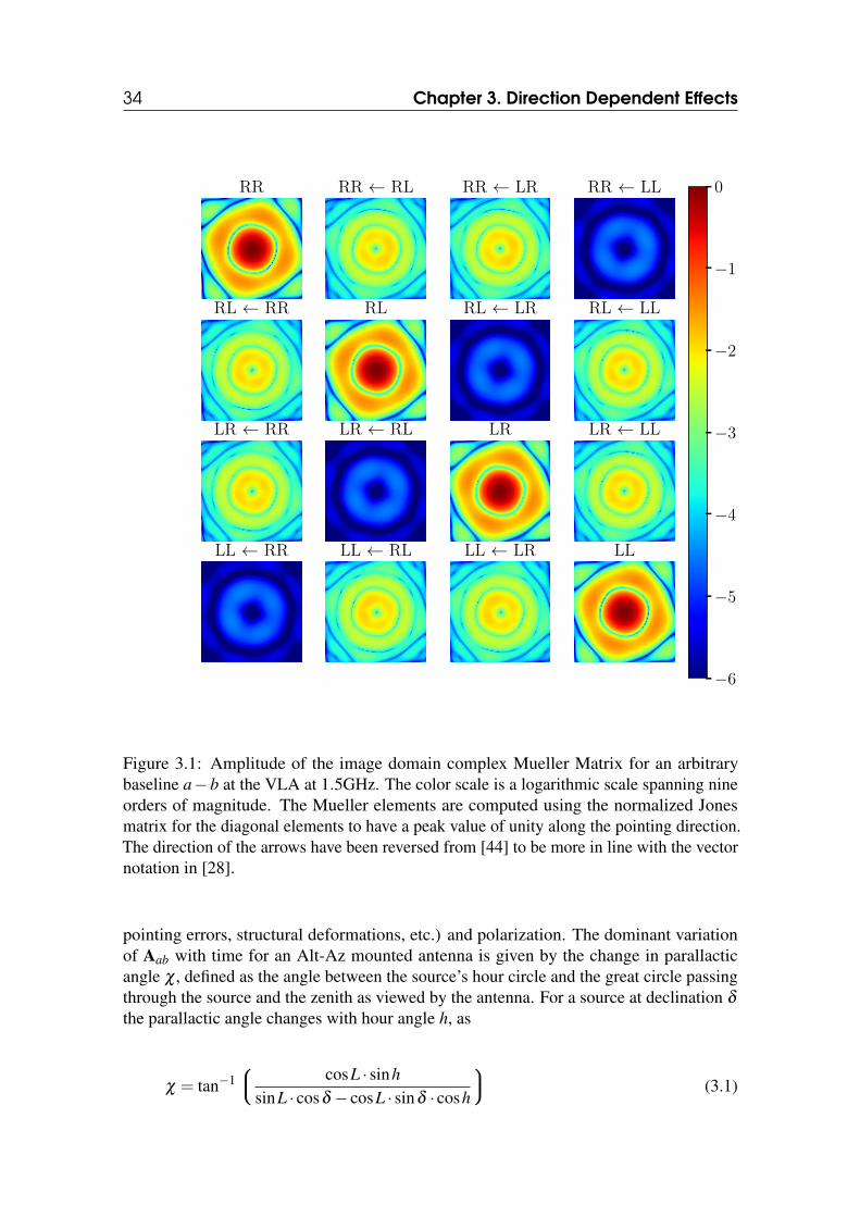
Figure 3.1: Amplitude of the image domain complex Mueller Matrix for an arbitrarybaseline a−b at the VLA at 1.5GHz. The color scale is a logarithmic scale spanning nineorders of magnitude. The Mueller elements are computed using the normalized Jonesmatrix for the diagonal elements to have a peak value of unity along the pointing direction.The direction of the arrows have been reversed from [44] to be more in line with the vectornotation in [28].
pointing errors, structural deformations, etc.) and polarization. The dominant variationof Aab with time for an Alt-Az mounted antenna is given by the change in parallacticangle χ , defined as the angle between the source’s hour circle and the great circle passingthrough the source and the zenith as viewed by the antenna. For a source at declination δ
the parallactic angle changes with hour angle h, as
χ = tan−1 cosL · sinh
sinL · cosδ − cosL · sinδ · cosh
(3.1)
3.2 Primary Beam as a Direction Dependent Effect 35
I I ← Q I ← U I ← V
Q ← I Q Q ← U Q ← V
U ← I U ← Q U U ← V
V ← I V ← Q V ← U V
−6
−4
−2
0
2
4
6
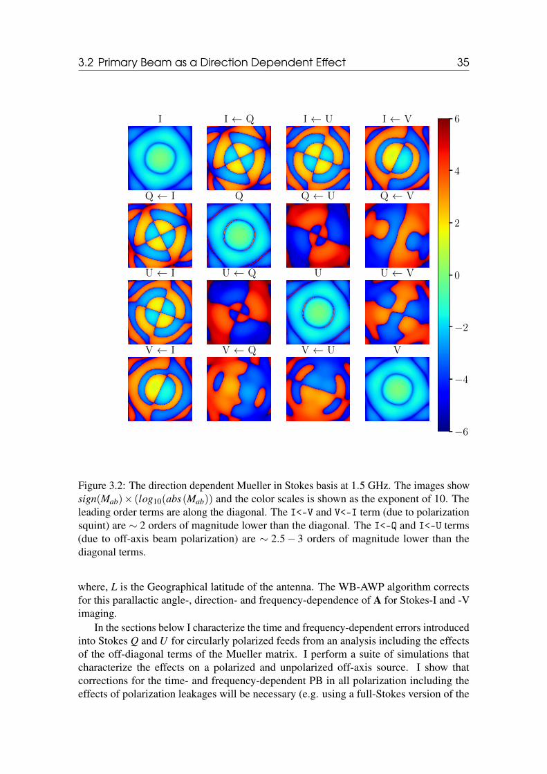
Figure 3.2: The direction dependent Mueller in Stokes basis at 1.5 GHz. The images showsign(Mab)× (log10(abs(Mab)) and the color scales is shown as the exponent of 10. Theleading order terms are along the diagonal. The I<-V and V<-I term (due to polarizationsquint) are ∼ 2 orders of magnitude lower than the diagonal. The I<-Q and I<-U terms(due to off-axis beam polarization) are ∼ 2.5− 3 orders of magnitude lower than thediagonal terms.
where, L is the Geographical latitude of the antenna. The WB-AWP algorithm correctsfor this parallactic angle-, direction- and frequency-dependence of A for Stokes-I and -Vimaging.
In the sections below I characterize the time and frequency-dependent errors introducedinto Stokes Q and U for circularly polarized feeds from an analysis including the effectsof the off-diagonal terms of the Mueller matrix. I perform a suite of simulations thatcharacterize the effects on a polarized and unpolarized off-axis source. I show thatcorrections for the time- and frequency-dependent PB in all polarization including theeffects of polarization leakages will be necessary (e.g. using a full-Stokes version of the
36 Chapter 3. Direction Dependent Effects
WB-AWP algorithm) for accurate reconstruction of the true full-Stokes flux density vectorin wide-field, wide-band imaging. In chapter 5 I will lay out the framework and workingsof the full-Stokes WB-AWP algorithm that corrects for the entire Mueller matrix duringimage reconstruction.
The measurement equation in the image-plane can be cast in Stokes basis as,
~IM = ∑k
Mk ·~I (3.2)
where k is an index over time, frequency, and baseline. The vector~I is the true incidentfull-Stokes sky brightness distribution. ~IM is the measured apparent sky brightness distri-bution. Mk encodes the response of the interferometer to the incident polarization vector.Expanding Mk in Eq. 3.2 shows explicitly the dependence on the incident polarization.
~IM = ∑k
Mk
III +MkIQQ+Mk
IUU +MkIVV
MkQII +Mk
QQQ+MkQUU +Mk
QVVMk
UII +MkUQQ+Mk
UUU +MkUVV
MkVII +Mk
VQQ+MkVUU +Mk
VVV
(3.3)
The diagonal of the Mueller matrix encodes the response of the interferometer pair toeach individual Stokes parameter. The off-diagonal elements encode the leakage betweenStokes parameters. Mk
IQ and MkIU encodes the amount of flux leaking from I into Q and
U respectively. Magnitude of leakage i.e. the fraction of flux leakage is ∼5×10⁻² of Ifor the VLA at L-band at the half power point (refer, Fig. 3.2), and grows with increasingdistance from the beam center. The typical linear polarized intensity of astrophysicalsources is at the level of a few percent of Stokes-I flux. Hence, the flux leakage resultsin a fractional error of up to 100% in the wide-band full-Stokes measurements of typicalastrophysical signals. It is noteworthy that the Mueller matrix element Mk
QI representingthe mutual coupling between Stokes Q and I, has exactly the same magnitude as Mk
IQ,within calibration errors. However, the amount of flux leakage is modulated by the intensityof the Stokes parameters. The amount of flux leaking from Stokes Q into I is Mk
IQ ·Q. Fora typical linear polarization of a few %, the magnitude of flux leaking from Stokes Q into Iis a 10−4−10−5, which will be of a concern only for very high dynamic range imaging.However, in cases of highly polarized emission such as may be seen in extended radiojets of some radio galaxies, leakage from Q to I of order 10−3 may occur in uncorrectedimages.
One can isolate the effects of leakage by recasting Eq. 3.2 into a sum of the diagonaland off-diagonal elements,
~IM = ∑a,ν ,t
Maa · Ia + ∑b,a6=b
MabIb
(3.4)
The first term is the direction-dependent PB responses in each Stokes parameter. Thesecond term isolates the direction-dependent leakage between Stokes flux leakage, whichfor linear polarization is dominated by the direction-dependent Stokes I leakage. Notethat for the time-variable component, all terms can be ignored and the second term isrepresented as a constant only for very short “snapshot” observations with Alt-Az antennas.
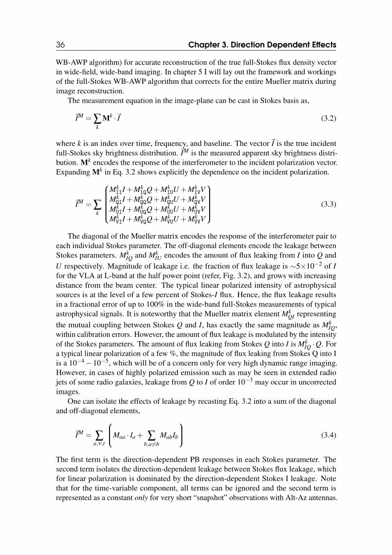
3.3 Simulations 37
Figure 3.3: The imaging simulations followed the methodology outlined in the flowdiagram. The sky model image was multiplied by the Fourier transform of the Muellermatrix for a change in parallactic angle of 5
This approach was used for the NVSS (Condon et al. [7]). Observations with equatorialmount antennas or antennas with the third axis of motion to maintain a fixed parallacticangle (McConnell et al. [46]) allow for a simple correction in the form of a direction-dependent flux subtraction post imaging. This technique was used to good effect for theCanadian Galactic Plane Survey (Taylor et al. [47] ) using the equatorial mount antennas ofthe Dominion Radio Astronomy Observatory synthesis radio telescope. For observationscovering a large parallactic range with Alt-Az antennas, these effects must be corrected aspart of the deconvolution and imaging stage.
3.3 SimulationsTo examine the characteristics of the errors in polarized signals and their effect on as-trophysical measurements I carried out a suite of simulations. In each case, I considera simple point source located at an off-axis point in the PB. This simple model allowsfor an intuitive understanding and interpretation of the resulting PB effects. Three caseswere considered. In the first case I consider the effect on an unpolarized point source.I then consider two polarized sources, one with zero Faraday Rotation Measure (RM)and the second with an RM of 100 rad m−2. These cases allow us to explore the effectsof the frequency dependence of the Mueller terms on Faraday Rotation synthesis. Thesimulations in all these cases utilized the ray-traced PBs using the implementation in theCASA R&D code base.
I simulated observations over an hour angle range of −4 hr to +4 hr and spanning1 GHz bandwidth in two frequency resolutions, the first with eight 128 MHz-wide spectralwindows across the VLA L-Band (1-2 GHz) to understand continuum polarization imagingfidelity. The second with 64 spectral windows with a bandwidth of 16 MHz each tounderstand the effects of antenna PB on Faraday rotation synthesis. The sources wereat Declination +70. An image domain sky model was created following Eq. 3.2. Thesky model was then used to create visibilities given by the Eq. 2.31 for the VLA in C-
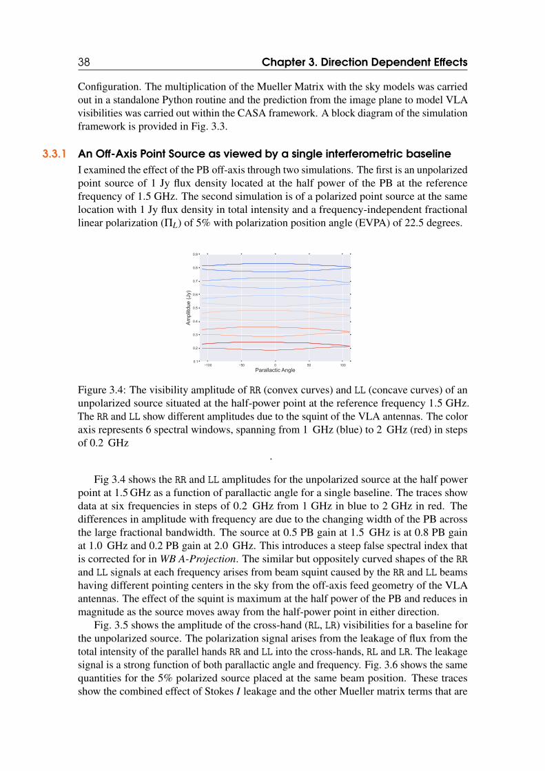
38 Chapter 3. Direction Dependent Effects
Configuration. The multiplication of the Mueller Matrix with the sky models was carriedout in a standalone Python routine and the prediction from the image plane to model VLAvisibilities was carried out within the CASA framework. A block diagram of the simulationframework is provided in Fig. 3.3.
3.3.1 An Off-Axis Point Source as viewed by a single interferometric baselineI examined the effect of the PB off-axis through two simulations. The first is an unpolarizedpoint source of 1 Jy flux density located at the half power of the PB at the referencefrequency of 1.5 GHz. The second simulation is of a polarized point source at the samelocation with 1 Jy flux density in total intensity and a frequency-independent fractionallinear polarization (ΠL) of 5% with polarization position angle (EVPA) of 22.5 degrees.
−100 −50 0 50 100Parallactic Angle
0.1
0.2
0.3
0.4
0.5
0.6
0.7
0.8
0.9
Amplitd
ue (J
y)
Figure 3.4: The visibility amplitude of RR (convex curves) and LL (concave curves) of anunpolarized source situated at the half-power point at the reference frequency 1.5 GHz.The RR and LL show different amplitudes due to the squint of the VLA antennas. The coloraxis represents 6 spectral windows, spanning from 1 GHz (blue) to 2 GHz (red) in stepsof 0.2 GHz
.
Fig 3.4 shows the RR and LL amplitudes for the unpolarized source at the half powerpoint at 1.5 GHz as a function of parallactic angle for a single baseline. The traces showdata at six frequencies in steps of 0.2 GHz from 1 GHz in blue to 2 GHz in red. Thedifferences in amplitude with frequency are due to the changing width of the PB acrossthe large fractional bandwidth. The source at 0.5 PB gain at 1.5 GHz is at 0.8 PB gainat 1.0 GHz and 0.2 PB gain at 2.0 GHz. This introduces a steep false spectral index thatis corrected for in WB A-Projection. The similar but oppositely curved shapes of the RRand LL signals at each frequency arises from beam squint caused by the RR and LL beamshaving different pointing centers in the sky from the off-axis feed geometry of the VLAantennas. The effect of the squint is maximum at the half power of the PB and reduces inmagnitude as the source moves away from the half-power point in either direction.
Fig. 3.5 shows the amplitude of the cross-hand (RL, LR) visibilities for a baseline forthe unpolarized source. The polarization signal arises from the leakage of flux from thetotal intensity of the parallel hands RR and LL into the cross-hands, RL and LR. The leakagesignal is a strong function of both parallactic angle and frequency. Fig. 3.6 shows the samequantities for the 5% polarized source placed at the same beam position. These tracesshow the combined effect of Stokes I leakage and the other Mueller matrix terms that are
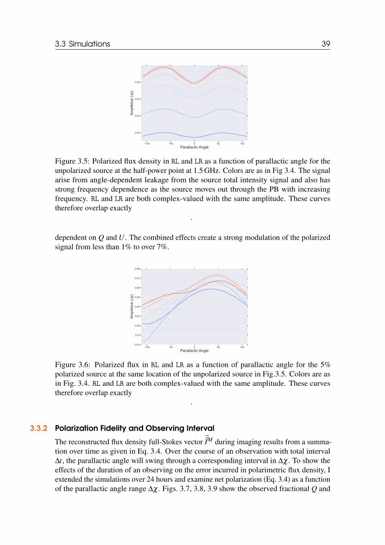
3.3 Simulations 39
−100 −50 0 50 100Parallactic Angle
0.02
0.03
0.04
0.05
Amplitd
ue (J
y)
Figure 3.5: Polarized flux density in RL and LR as a function of parallactic angle for theunpolarized source at the half-power point at 1.5 GHz. Colors are as in Fig 3.4. The signalarise from angle-dependent leakage from the source total intensity signal and also hasstrong frequency dependence as the source moves out through the PB with increasingfrequency. RL and LR are both complex-valued with the same amplitude. These curvestherefore overlap exactly
.
dependent on Q and U . The combined effects create a strong modulation of the polarizedsignal from less than 1% to over 7%.
−100 −50 0 50 100Parallactic Angle
0.00
0.01
0.02
0.03
0.04
0.05
0.06
0.07
0.08
Amplitd
ue (J
y)
Figure 3.6: Polarized flux in RL and LR as a function of parallactic angle for the 5%polarized source at the same location of the unpolarized source in Fig.3.5. Colors are asin Fig. 3.4. RL and LR are both complex-valued with the same amplitude. These curvestherefore overlap exactly
.
3.3.2 Polarization Fidelity and Observing Interval
The reconstructed flux density full-Stokes vector~~IM during imaging results from a summa-tion over time as given in Eq. 3.4. Over the course of an observation with total interval∆t, the parallactic angle will swing through a corresponding interval in ∆χ . To show theeffects of the duration of an observing on the error incurred in polarimetric flux density, Iextended the simulations over 24 hours and examine net polarization (Eq. 3.4) as a functionof the parallactic angle range ∆χ . Figs. 3.7, 3.8, 3.9 show the observed fractional Q and
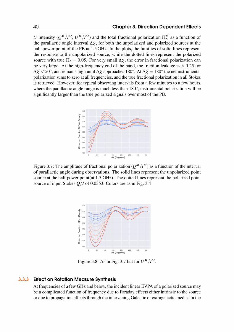
40 Chapter 3. Direction Dependent Effects
U intensity (QM/IM, UM/IM) and the total fractional polarization ΠML as a function of
the parallactic angle interval ∆χ , for both the unpolarized and polarized sources at thehalf-power point of the PB at 1.5 GHz. In the plots, the families of solid lines representthe response to the unpolarized source, while the dotted lines represent the polarizedsource with true ΠL = 0.05. For very small ∆χ , the error in fractional polarization canbe very large. At the high-frequency end of the band, the fraction leakage is > 0.25 for∆χ < 50, and remains high until ∆χ approaches 180. At ∆χ = 180 the net instrumentalpolarization sums to zero at all frequencies, and the true fractional polarization in all Stokesis retrieved. However, for typical observing intervals from a few minutes to a few hours,where the parallactic angle range is much less than 180, instrumental polarization will besignificantly larger than the true polarized signals over most of the PB.
0 50 100 150 200 250 300 350
Δχ (degrees)−0.25
−0.20
−0.15
−0.10
−0.05
0.00
0.05
0.10
0.15
Obs
erve
d Frac
tion Q Flux Den
sity
Figure 3.7: The amplitude of fractional polarization (QM/IM) as a function of the intervalof parallactic angle during observations. The solid lines represent the unpolarized pointsource at the half power point(at 1.5 GHz). The dotted lines represent the polarized pointsource of input Stokes Q/I of 0.0353. Colors are as in Fig. 3.4
0 50 100 150 200 250 300 350
Δχ (degrees)
−0.30
−0.25
−0.20
−0.15
−0.10
−0.05
0.00
0.05
Obs
erve
d Frac
tion U Flux Den
sity
Figure 3.8: As in Fig. 3.7 but for UM/IM.
3.3.3 Effect on Rotation Measure SynthesisAt frequencies of a few GHz and below, the incident linear EVPA of a polarized source maybe a complicated function of frequency due to Faraday effects either intrinsic to the sourceor due to propagation effects through the intervening Galactic or extragalactic media. In the
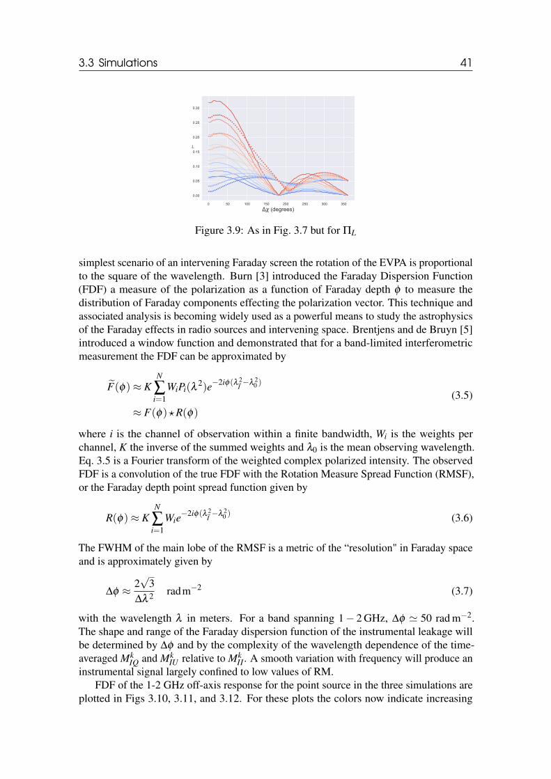
3.3 Simulations 41
0 50 100 150 200 250 300 350
Δχ (degrees)
0.00
0.05
0.10
0.15
0.20
0.25
0.30
πL
Figure 3.9: As in Fig. 3.7 but for ΠL
simplest scenario of an intervening Faraday screen the rotation of the EVPA is proportionalto the square of the wavelength. Burn [3] introduced the Faraday Dispersion Function(FDF) a measure of the polarization as a function of Faraday depth φ to measure thedistribution of Faraday components effecting the polarization vector. This technique andassociated analysis is becoming widely used as a powerful means to study the astrophysicsof the Faraday effects in radio sources and intervening space. Brentjens and de Bruyn [5]introduced a window function and demonstrated that for a band-limited interferometricmeasurement the FDF can be approximated by
F(φ)≈ KN
∑i=1
WiPi(λ2)e−2iφ(λ 2
~I−λ 2
0 )
≈ F(φ)?R(φ)
(3.5)
where i is the channel of observation within a finite bandwidth, Wi is the weights perchannel, K the inverse of the summed weights and λ0 is the mean observing wavelength.Eq. 3.5 is a Fourier transform of the weighted complex polarized intensity. The observedFDF is a convolution of the true FDF with the Rotation Measure Spread Function (RMSF),or the Faraday depth point spread function given by
R(φ)≈ KN
∑i=1
Wie−2iφ(λ 2
~I−λ 2
0 ) (3.6)
The FWHM of the main lobe of the RMSF is a metric of the “resolution" in Faraday spaceand is approximately given by
∆φ ≈ 2√
3∆λ 2 radm−2 (3.7)
with the wavelength λ in meters. For a band spanning 1− 2 GHz, ∆φ ' 50 rad m−2.The shape and range of the Faraday dispersion function of the instrumental leakage willbe determined by ∆φ and by the complexity of the wavelength dependence of the time-averaged Mk
IQ and MkIU relative to Mk
II . A smooth variation with frequency will produce aninstrumental signal largely confined to low values of RM.
FDF of the 1-2 GHz off-axis response for the point source in the three simulations areplotted in Figs 3.10, 3.11, and 3.12. For these plots the colors now indicate increasing
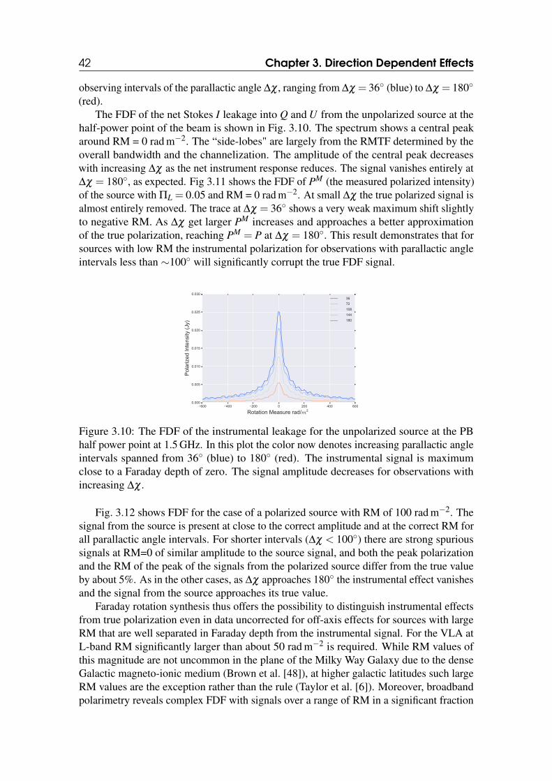
42 Chapter 3. Direction Dependent Effects
observing intervals of the parallactic angle ∆χ , ranging from ∆χ = 36 (blue) to ∆χ = 180
(red).The FDF of the net Stokes I leakage into Q and U from the unpolarized source at the
half-power point of the beam is shown in Fig. 3.10. The spectrum shows a central peakaround RM = 0 rad m−2. The “side-lobes" are largely from the RMTF determined by theoverall bandwidth and the channelization. The amplitude of the central peak decreaseswith increasing ∆χ as the net instrument response reduces. The signal vanishes entirely at∆χ = 180, as expected. Fig 3.11 shows the FDF of PM (the measured polarized intensity)of the source with ΠL = 0.05 and RM = 0 rad m−2. At small ∆χ the true polarized signal isalmost entirely removed. The trace at ∆χ = 36 shows a very weak maximum shift slightlyto negative RM. As ∆χ get larger PM increases and approaches a better approximationof the true polarization, reaching PM = P at ∆χ = 180. This result demonstrates that forsources with low RM the instrumental polarization for observations with parallactic angleintervals less than ∼100 will significantly corrupt the true FDF signal.
−600 −400 −200 0 200 400 600
Rotation Measure rad/m2
0.000
0.005
0.010
0.015
0.020
0.025
0.030
Polarized
Intens
ity (J
y)
∆χ 36∆χ 72∆χ 108∆χ 144∆χ 180
Figure 3.10: The FDF of the instrumental leakage for the unpolarized source at the PBhalf power point at 1.5 GHz. In this plot the color now denotes increasing parallactic angleintervals spanned from 36 (blue) to 180 (red). The instrumental signal is maximumclose to a Faraday depth of zero. The signal amplitude decreases for observations withincreasing ∆χ .
Fig. 3.12 shows FDF for the case of a polarized source with RM of 100 rad m−2. Thesignal from the source is present at close to the correct amplitude and at the correct RM forall parallactic angle intervals. For shorter intervals (∆χ < 100) there are strong spurioussignals at RM=0 of similar amplitude to the source signal, and both the peak polarizationand the RM of the peak of the signals from the polarized source differ from the true valueby about 5%. As in the other cases, as ∆χ approaches 180 the instrumental effect vanishesand the signal from the source approaches its true value.
Faraday rotation synthesis thus offers the possibility to distinguish instrumental effectsfrom true polarization even in data uncorrected for off-axis effects for sources with largeRM that are well separated in Faraday depth from the instrumental signal. For the VLA atL-band RM significantly larger than about 50 rad m−2 is required. While RM values ofthis magnitude are not uncommon in the plane of the Milky Way Galaxy due to the denseGalactic magneto-ionic medium (Brown et al. [48]), at higher galactic latitudes such largeRM values are the exception rather than the rule (Taylor et al. [6]). Moreover, broadbandpolarimetry reveals complex FDF with signals over a range of RM in a significant fraction
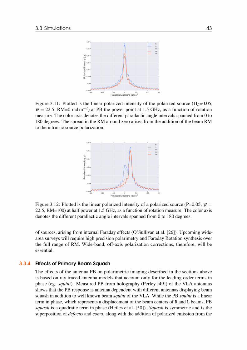
3.3 Simulations 43
−600 −400 −200 0 200 400 600
Rotation Measure rad/m2
0.00
0.01
0.02
0.03
0.04
0.05
0.06
0.07
Polarized
Intens
ity (J
y)
∆χ 36∆χ 72∆χ 108∆χ 144∆χ 180
Figure 3.11: Plotted is the linear polarized intensity of the polarized source (ΠL=0.05,ψ = 22.5, RM=0 rad m−2) at PB the power point at 1.5 GHz, as a function of rotationmeasure. The color axis denotes the different parallactic angle intervals spanned from 0 to180 degrees. The spread in the RM around zero arises from the addition of the beam RMto the intrinsic source polarization.
−600 −400 −200 0 200 400 600
Rotation Measure rad/m2
0.00
0.01
0.02
0.03
0.04
0.05
0.06
Polarized
Intens
ity (J
y)
∆χ 36∆χ 72∆χ 108∆χ 144∆χ 180
Figure 3.12: Plotted is the linear polarized intensity of a polarized source (P=0.05, ψ =22.5, RM=100) at half power at 1.5 GHz, as a function of rotation measure. The color axisdenotes the different parallactic angle intervals spanned from 0 to 180 degrees.
of sources, arising from internal Faraday effects (O’Sullivan et al. [26]). Upcoming wide-area surveys will require high precision polarimetry and Faraday Rotation synthesis overthe full range of RM. Wide-band, off-axis polarization corrections, therefore, will beessential.
3.3.4 Effects of Primary Beam Squash
The effects of the antenna PB on polarimetric imaging described in the sections aboveis based on ray traced antenna models that account only for the leading order terms inphase (eg. squint). Measured PB from holography (Perley [49]) of the VLA antennasshows that the PB response is antenna dependent with different antennas displaying beamsquash in addition to well known beam squint of the VLA. While the PB squint is a linearterm in phase, which represents a displacement of the beam centers of R and L beams, PBsquash is a quadratic term in phase (Heiles et al. [50]). Squash is symmetric and is thesuperposition of defocus and coma, along with the addition of polarized emission from the
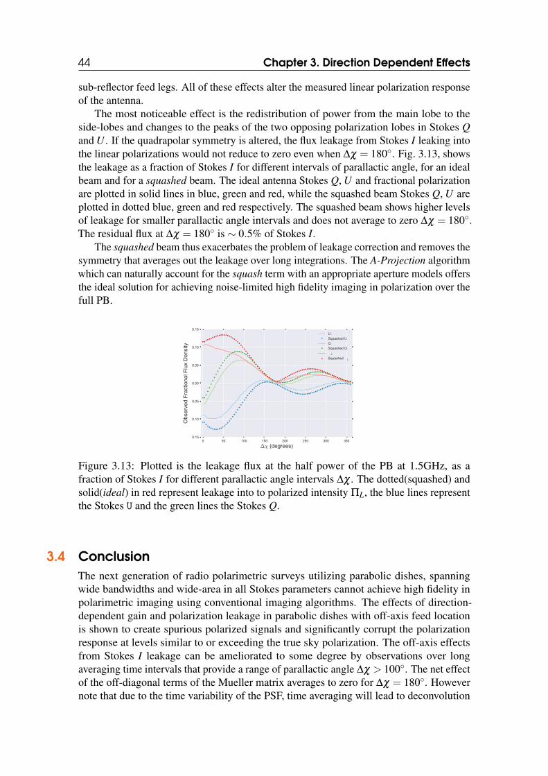
44 Chapter 3. Direction Dependent Effects
sub-reflector feed legs. All of these effects alter the measured linear polarization responseof the antenna.
The most noticeable effect is the redistribution of power from the main lobe to theside-lobes and changes to the peaks of the two opposing polarization lobes in Stokes Qand U . If the quadrapolar symmetry is altered, the flux leakage from Stokes I leaking intothe linear polarizations would not reduce to zero even when ∆χ = 180. Fig. 3.13, showsthe leakage as a fraction of Stokes I for different intervals of parallactic angle, for an idealbeam and for a squashed beam. The ideal antenna Stokes Q, U and fractional polarizationare plotted in solid lines in blue, green and red, while the squashed beam Stokes Q, U areplotted in dotted blue, green and red respectively. The squashed beam shows higher levelsof leakage for smaller parallactic angle intervals and does not average to zero ∆χ = 180.The residual flux at ∆χ = 180 is ∼ 0.5% of Stokes I.
The squashed beam thus exacerbates the problem of leakage correction and removes thesymmetry that averages out the leakage over long integrations. The A-Projection algorithmwhich can naturally account for the squash term with an appropriate aperture models offersthe ideal solution for achieving noise-limited high fidelity imaging in polarization over thefull PB.
0 50 100 150 200 250 300 350
∆χ (degrees)
−0.15
−0.10
−0.05
0.00
0.05
0.10
0.15
Obs
erve
d Frac
tiona
l Flu Den
sity
USquashed UQSquashed QΠL
Squashed ΠL
Figure 3.13: Plotted is the leakage flux at the half power of the PB at 1.5GHz, as afraction of Stokes I for different parallactic angle intervals ∆χ . The dotted(squashed) andsolid(ideal) in red represent leakage into to polarized intensity ΠL, the blue lines representthe Stokes U and the green lines the Stokes Q.
3.4 ConclusionThe next generation of radio polarimetric surveys utilizing parabolic dishes, spanningwide bandwidths and wide-area in all Stokes parameters cannot achieve high fidelity inpolarimetric imaging using conventional imaging algorithms. The effects of direction-dependent gain and polarization leakage in parabolic dishes with off-axis feed locationis shown to create spurious polarized signals and significantly corrupt the polarizationresponse at levels similar to or exceeding the true sky polarization. The off-axis effectsfrom Stokes I leakage can be ameliorated to some degree by observations over longaveraging time intervals that provide a range of parallactic angle ∆χ > 100. The net effectof the off-diagonal terms of the Mueller matrix averages to zero for ∆χ = 180. Howevernote that due to the time variability of the PSF, time averaging will lead to deconvolution

3.4 Conclusion 45
errors during image reconstruction. Observations that do not span such long time intervalsor cover exactly symmetric hour angles about the meridian, the polarization leakage doesnot vanish. I have also shown that for realistic beam models with measurable second-ordererrors (beam squash) averaging of polarization leakage is not a viable solution.
The off-axis instrumental polarization response of the antenna in Faraday space isshown to be close to RM of 0 rad m−2. For typical RM signatures of astrophysical sourcesat GHz frequencies the off-axis leakage response alters the Faraday dispersion spectrum,introducing spurious signals similar in scale to the sky polarization and corrupting the truesky RM signature. Our simulations show that achieving polarimetric imaging simultane-ously over wide-fields and wide-bands for next-generation deep and wide surveys will notbe possible through conventional imaging methods that do not include DD corrections.

46 Chapter 3. Direction Dependent Effects
4. Antenna Aperture Illumination
The aperture illumination pattern (AIP) of an antenna determines the directional gain andsensitivity of the antenna to the sky brightness distribution. For an interferometric baselineconsisting of a pair of antennas, the outer convolution of the two AIPs determines theMueller matrix. The Mueller matrix encodes the mixing of the input polarization signals,including the effects of the off-axis leakage of one polarization product into another. Italso largely determines the imaging performance. Accurate knowledge of the antenna AIPis essential for high-fidelity imaging performance of a radio interferometric array.
The current and next generation of interferometric arrays are outfitted with dual-polarization, wide-bandwidth receivers having high fractional bandwidths (Total band-width/center frequency), e.g. in the case of the VLA, by as much as 66–75% (L, S, and Cbands). The directional properties of the AIP in each polarization will change significantlyacross the band. In addition to smoothly varying geometric frequency scaling of the AIP,effects can arise due to, imperfect optical alignments or standing waves between opticalelements of the antenna (e.g. Popping and Braun [51]). Standard calibration and imagingalgorithms that do not account for the directional and frequency dependence of the antennaAIP lead to errors whose magnitude increases with distance from the antenna pointingdirection and are particularly significant for polarization imaging (Jagannathan et al. [52]).With a known AIP, the direction-dependent errors can be corrected over the field-of-viewusing the A-Projection algorithm (Bhatnagar et al. [32, 33]).
The AIP can be modeled to the first order by a simple ray-tracing geometric model.Geometric models of aperture illumination deliver sufficient accuracy in the regime wherethe incident wavelength of electro-magnetic waves is much smaller than the blockingantenna structures in the optical path. At its highest operation frequencies of 10s of GHz,the VLA falls in this geometric regime. However at GHz frequencies and lower purelygeometric approaches are insufficient, higher order effects from diffraction and, scatteringsignificantly affect and alter the AIP. These effects introduce higher order frequency-dependent terms. Full Electromagnetic (EM) simulations of the antenna in principle
48 Chapter 4. Antenna Aperture Illumination
allow for the accurate modeling of the AIP including higher order effects (Brisken [53]).However such approaches are computationally expensive (even more for high spectralresolution simulation across wide bandwidths) and are limited by the accuracy of antennamodels and illumination patterns which are given as an initial input. Results from such EMsimulations often do not accurately reflect the real AIPs and are difficult (and expensive)to perturb to fit the measured AIPs. In this chapter, I describe a hybrid method, called theA-solver, that uses holographic measurements in combination with low-order parametricmodeling based on the physical structure of the antennas to efficiently create a high spectralresolution model of the full-polarization AIP over the very wide-bandwidth of the VLA.
4.1 A-Solver4.1.1 Physical Modeling of the AIP
Approaches to computer models of the AIP or the antenna voltage pattern (VP) can bebroadly classified as Physical Modeling or Phenomenological Modeling. While a detaileddiscussion of these styles of modeling is beyond the scope of this discussion, I would liketo mention here that Physical Modeling (e.g. simulators using Physical Optics (PO) orfull-EM simulators) minimizes the required degrees-of-freedom in the model and followsthe physics of the problem, both of which have significant numerical and computationaladvantages. Physical Modeling also leads to a fundamental understanding of the instrument.Phenomenological modeling on the other hand1 ignores physics and models individualeffects as free parameters.
A simple model of the far-field radiation pattern can be computed using geometricoptics (GO). This works well for smooth surfaces away from edges and structures that aremuch smaller than the wavelength of radiation, where diffractive effects become important.For observations above several GHz with the VLA, diffractive effects are expected to besmall (e.g. see Bhatnagar et al. [32] where instrumental Stokes-V is modeled using a GOsimulator for the VP). An adaptation of a GO simulator [53] exists in CASA, and referredto as the “CASSBEAM” simulator. The code though VLA centric is general and can beused to model Cassegrain antennas in general. The simulator takes as input a parametricdescription of the structure of the antenna. The VLA antennas are shaped Cassegrainsystem, with a nearly parabolic primary and a hyperbolic secondary designed to attain amore uniform illumination of the antenna aperture. The shaped aperture alters the side-lobelevels of the antenna far-field, and the side-lobe azimuthal symmetry is altered by thepresence of the quadrupod legs holding up the secondary. The general shape of the mainlobe and the side lobes is also altered by the central blockage due to the sub-reflector.
The set of parameters used in our work to describe the structure and optics of a VLAantenna are shown in Fig. 4.1 and are listed in Table 4.1. The shape of the secondaryreflector is not part of the model and is computed on-the-fly during ray tracing by enforcingthe optical path length of the rays to be a constant, from the time of the first incidence. Thealgorithm computes the changes in the electric field for the different reflections, followingthe rays to the feed where the electric fields in a natural linear polarization basis are
1An extreme example of this in radio interferometric imaging is the Peeling approach where eachcomponent of the sky brightness distribution is modeled separately, parameterized to separately accountfor each effect, like polarization squint, antenna pointing offset, the dependence of beam shapes with time,frequency and polarization, amongst others.
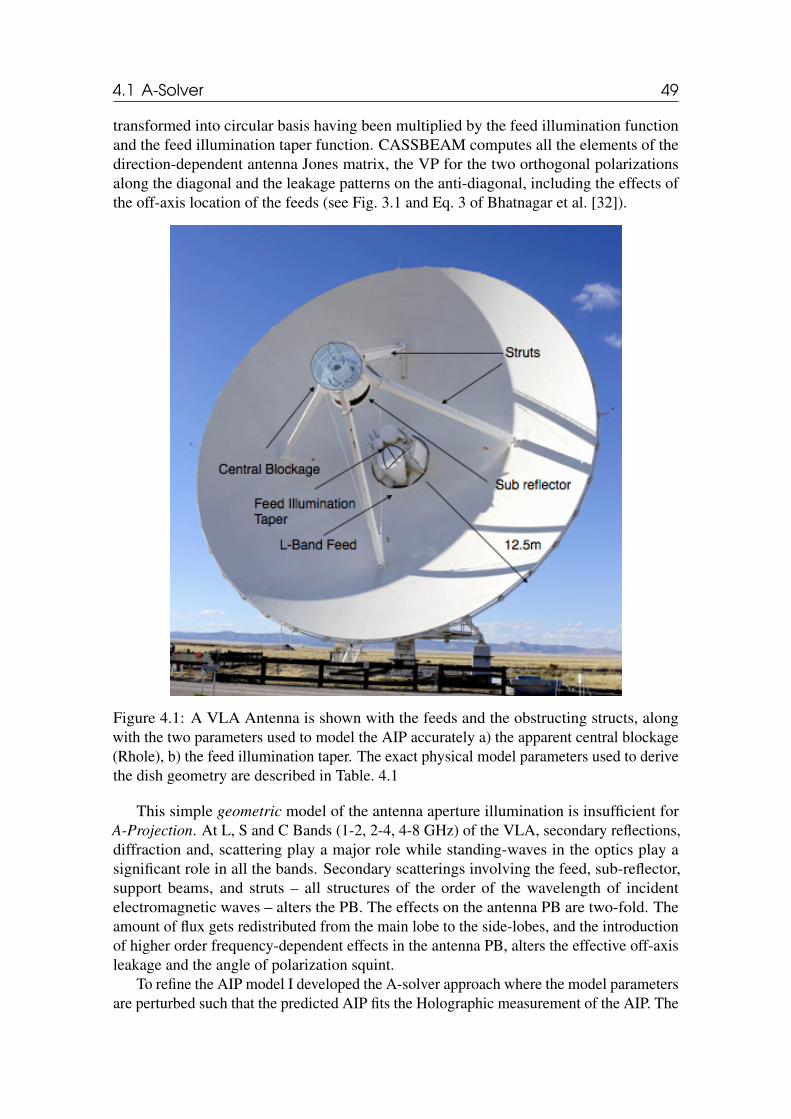
4.1 A-Solver 49
transformed into circular basis having been multiplied by the feed illumination functionand the feed illumination taper function. CASSBEAM computes all the elements of thedirection-dependent antenna Jones matrix, the VP for the two orthogonal polarizationsalong the diagonal and the leakage patterns on the anti-diagonal, including the effects ofthe off-axis location of the feeds (see Fig. 3.1 and Eq. 3 of Bhatnagar et al. [32]).
Figure 4.1: A VLA Antenna is shown with the feeds and the obstructing structs, alongwith the two parameters used to model the AIP accurately a) the apparent central blockage(Rhole), b) the feed illumination taper. The exact physical model parameters used to derivethe dish geometry are described in Table. 4.1
This simple geometric model of the antenna aperture illumination is insufficient forA-Projection. At L, S and C Bands (1-2, 2-4, 4-8 GHz) of the VLA, secondary reflections,diffraction and, scattering play a major role while standing-waves in the optics play asignificant role in all the bands. Secondary scatterings involving the feed, sub-reflector,support beams, and struts – all structures of the order of the wavelength of incidentelectromagnetic waves – alters the PB. The effects on the antenna PB are two-fold. Theamount of flux gets redistributed from the main lobe to the side-lobes, and the introductionof higher order frequency-dependent effects in the antenna PB, alters the effective off-axisleakage and the angle of polarization squint.
To refine the AIP model I developed the A-solver approach where the model parametersare perturbed such that the predicted AIP fits the Holographic measurement of the AIP. The
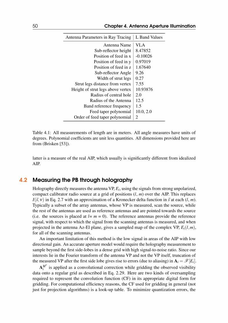
50 Chapter 4. Antenna Aperture Illumination
Antenna Parameters in Ray Tracing L Band Values
Antenna Name VLASub-reflector height 8.47852Position of feed in x -0.10026Position of feed in y 0.97019Position of feed in z 1.67640Sub-reflector Angle 9.26Width of strut legs 0.27
Strut legs distance from vertex 7.55Height of strut legs above vertex 10.93876
Radius of central hole 2.0Radius of the Antenna 12.5
Band reference frequency 1.5Feed taper polynomial 10.0, 2.0
Order of feed taper polynomial 2
Table 4.1: All measurements of length are in meters. All angle measures have units ofdegrees. Polynomial coefficients are unit less quantities. All dimensions provided here arefrom (Brisken [53]).
latter is a measure of the real AIP, which usually is significantly different from idealizedAIP.
4.2 Measuring the PB through holographyHolography directly measures the antenna VP, Ei, using the signals from strong unpolarized,compact calibrator radio source at a grid of positions (l, m) over the AIP. This replacesI(~s,ν) in Eq. 2.7 with an approximation of a Kronecker delta function in~s at each (l, m).Typically a subset of the array antennas, whose VP is measured, scan the source, whilethe rest of the antennas are used as reference antennas and are pointed towards the source(i.e. the sources is placed at l= m = 0). The reference antennas provide the referencesignal, with respect to which the signal from the scanning antennas is measured, and whenprojected in the antenna Az-El plane, gives a sampled map of the complex VP, Ei(l,m),for all of the scanning antennas.
An important limitation of this method is the low signal in areas of the AIP with lowdirectional gain. An accurate aperture model would require the holography measurement tosample beyond the first side-lobes in a dense grid with high signal-to-noise ratio. Since ourinterests lie in the Fourier transform of the antenna VP and not the VP itself, truncation ofthe measured VP after the first side lobe gives rise to errors (due to aliasing) in Ai =F [Ei].
AM†
i is applied as a convolutional correction while gridding the observed visibilitydata onto a regular grid as described in Eq. 2.29. Here are two kinds of oversamplingrequired to represent the convolution function (CF) in its appropriate digital form forgridding. For computational efficiency reasons, the CF used for gridding in general (notjust for projection algorithms) is a look-up table. To minimize quantization errors, the
4.3 Optimizing the model through holography 51
CF look-up table needs to be oversampled by a factor represented by the symbol Oap(typically Oap ≥ 20). Holographic measurements are the measurements of the antenna VP(Ei) itself. To minimize aliasing as well as to measure the various features of the antennaVP accurately, the holographic measurements are also oversampled. However, due topractical limitations, a much smaller oversampling factor (1.5×) was used and found tobe sufficient for these antenna VP measurements. Since the holographic oversamplingfactor in the antenna VP measurement is much less than the oversampling factor neededfor gridding (Oap), a parameterized model of the antenna AIP is required.
4.2.1 HolographyFor the holography data used here, an unpolarized source, 3C147 (< 0.04% polarized),was scanned in a 35×35 grid in the antenna reference frame with a step size of ∆l,∆m =2.5057′, out to the second null (at 1GHz). In addition, a polarized calibrator 3C286was observed to provide polarization angle calibration. Half the array was utilized asreference antennas while the other target antennas scanned the array. For more details onthe holographic measurement see Perley [49].
The visibility data were imported into AIPS to obtain the antenna grid coordinates(l,m) for each holography scan. The uncalibrated data were exported as UVFITS file andimported into CASA as a Measurement Set. The calibrator fluxes were set using [54] and[55] for both 3C147 and 3C286 in all polarizations across the full bandwidth. On-axisgain, bandpass, frequency-dependent polarization leakage and polarization position anglecalibration were carried out and the calibration solutions were applied to the data using theAPPLYCAL task in CASA. Subsequently, utilizing the CASA toolkit, data from baselinesbetween the target antennas and each of the reference antennas were averaged to improvethe signal-to-noise ratio of the measured VPs. Further, the data recorded on a grid pointfor 10 seconds was averaged. This gave the final set of antenna VP data per channelper holography grid. The VP data were then interpolated onto a 128×128 grid on a perchannel basis to create a 1024-channel image cube for each of the target antennas, inpolarizations R and L (the diagonal elements of the DD antenna Jones matrix) and leakagepatterns R←L, L←R (the anti-diagonal elements of DD antenna Jones matrix).
4.3 Optimizing the model through holographyThe ray-tracing AIP simulator code within the CASA imaging R&D code base wasmodified to accept input parameters from a Python wrapper code. This was wrapped as aparameterized function in Python and utilized as the unknown function to be determined bythe Nelder-Mead simplex algorithm (Nelder and Mead [56]), minimizing for the functionparameters against each of the individual channel images of the target antenna VP cubeproduced from the holography data (see Section 4.2.1). The optimization parameters werethe apparent blockage (Rhole), the feed illumination taper function (ftaper as a 4th orderpolynomial), and the antenna pointing offset in R.A. and Dec (xoffset, yoffset)2. Thesimplex algorithm traversed each parameter space independent of the others varying themuntil a joint minima is found. The residuals before and after the joint minimization are
2The antenna pointing offset solved for is the mechanical antenna pointing, different from pointing offsetsdue to polarization squint. The latter is an optical phenomenon and is naturally included in the computationof the VP due to the physics of off-axis optics and does not need to be solved-for as an independent parameter
52 Chapter 4. Antenna Aperture Illumination
shown in the upper and lower panels of Fig. 4.2. The choice of the simplex algorithm overmore computationally optimal algorithms arises from the lack of apriori knowledge ofthe gradients of the various minimization parameters, in the seven-dimensional parameterspace.
The CASSBEAM code uses OpenMP thread parallelization and was set to launch fourthreads per process call. This parallelization allowed for the fast production of a new beammodel for every convergence iteration. Despite this parallelization, the minimization takes4 hours per channel per polarization to converge to a solution. So a serial minimizationwould take 2×1024×4 hours to derive a channelized solution for an antenna. Since eachchannel minimization based on the parameterization is independent of the next channel asimple frequency-based parallelization was used to trigger a parallel minimization run of1024 channels and two polarizations on the Amazon Web Services (AWS) compute cluster.This reduced the compute time down to 6 hours per antenna. The results for three antennasare discussed below. One should note here that the run-time would be unreasonably long ifa full Physical Optics simulator like GRASP 3 was used instead.
In order to highlight the efficacy of the parameterized model of AM~I
as against the idealmodel of the AIP’s Fig. 4.2 shows a comparison between |EHolo
~I−F †Aideal
~I| (top row)
and the |EHolo~I−F †AM
~I| (bottom row). Aideal
~Irefers to the default aperture illumination
produced by the CASSBEAM code, and AM~I
is derived from the parameter values obtainedby the optimization procedure discussed in Sec. 4.3. The first side-lobe is underestimatedin the upper panels of Fig. 4.2 by 50% in both polarizations (L upper left and R upper right).Within the main-lobe of the VP, the residuals in the upper panel show a systematic offsetin power within the main-lobe in both polarizations. The offset within the main-lobesthat affects both polarizations equally is a sign of mechanical antenna pointing error. Incontrast, the lower panel images (lower-left for L lower left and lower right for R lowerright) of the parameterized model residuals shows no sign of side-lobe power discrepancyor residual pointing error. These are residuals for one frequency channel. The optimizedresiduals show similar improvement across the entire bandwidth at the VLA L-Band forall the optimized antennas.
The optimization procedure solved for the pointing offset of the antenna and then fittedthe data for Rhole – the apparent blockage. Heiles et al. [50] demonstrated that a blockedaperture leads to increased power in the side-lobes. They also show that the size and extentof the VP side-lobes can be effectively shaped by tapering the illumination of the feeds. Inline with their finding, I was able to effectively model the first side-lobe power alteringthe apparent blockage in ray-tracing in conjunction with the ftaper, feed illuminationtaper polynomial function utilized in the code. I find that an increased apparent blockageand a sharper tapering function for feed illumination, determined per channel across theentire band allows for the capture of all significant changes in the antenna VP out thefirst side-lobe. I also note that the trend captured in the optimized parameters correlateswith the measured wide-band sensitivity of the VLA L-Band Momjian et al. [57], whichsuggests that the optimized models correctly estimate the departures from an idealizedantenna.
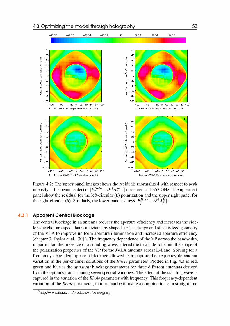
4.3 Optimizing the model through holography 53
Figure 4.2: The upper panel images shows the residuals (normalized with respect to peakintensity at the beam center) of |EHolo
~I−F †Aideal
~I| measured at 1.353 GHz. The upper left
panel show the residual for the left-circular (L) polarization and the upper right panel forthe right-circular (R). Similarly, the lower panels shows |EHolo
~I−F †AM
~I|.
4.3.1 Apparent Central BlockageThe central blockage in an antenna reduces the aperture efficiency and increases the side-lobe levels – an aspect that is alleviated by shaped surface design and off-axis feed geometryof the VLA to improve uniform aperture illumination and increased aperture efficiency(chapter 3, Taylor et al. [30] ). The frequency dependence of the VP across the bandwidth,in particular, the presence of a standing wave, altered the first side-lobe and the shape ofthe polarization properties of the VP for the JVLA antenna across L-Band. Solving for afrequency-dependent apparent blockage allowed us to capture the frequency-dependentvariation in the per-channel solutions of the Rhole parameter. Plotted in Fig. 4.3 in red,green and blue is the apparent blockage parameter for three different antennas derivedfrom the optimization spanning seven spectral windows. The effect of the standing wave iscaptured in the variation of the Rhole parameter with frequency. This frequency-dependentvariation of the Rhole parameter, in turn, can be fit using a combination of a straight line
3http://www.ticra.com/products/software/grasp
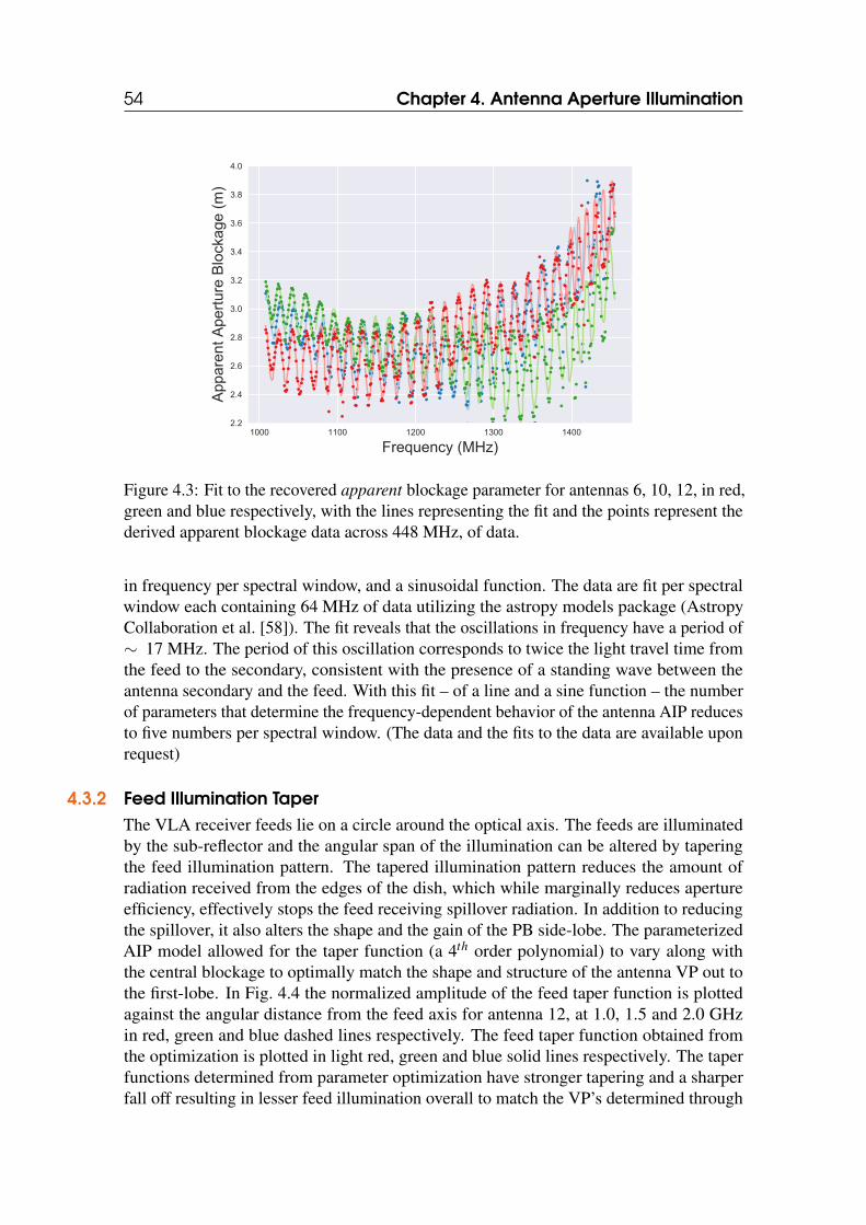
54 Chapter 4. Antenna Aperture Illumination
1000 1100 1200 1300 1400
Frequency (MHz)
2.2
2.4
2.6
2.8
3.0
3.2
3.4
3.6
3.8
4.0
App
aren
t Ape
rture Blockag
e (m
)
Figure 4.3: Fit to the recovered apparent blockage parameter for antennas 6, 10, 12, in red,green and blue respectively, with the lines representing the fit and the points represent thederived apparent blockage data across 448 MHz, of data.
in frequency per spectral window, and a sinusoidal function. The data are fit per spectralwindow each containing 64 MHz of data utilizing the astropy models package (AstropyCollaboration et al. [58]). The fit reveals that the oscillations in frequency have a period of∼ 17 MHz. The period of this oscillation corresponds to twice the light travel time fromthe feed to the secondary, consistent with the presence of a standing wave between theantenna secondary and the feed. With this fit – of a line and a sine function – the numberof parameters that determine the frequency-dependent behavior of the antenna AIP reducesto five numbers per spectral window. (The data and the fits to the data are available uponrequest)
4.3.2 Feed Illumination TaperThe VLA receiver feeds lie on a circle around the optical axis. The feeds are illuminatedby the sub-reflector and the angular span of the illumination can be altered by taperingthe feed illumination pattern. The tapered illumination pattern reduces the amount ofradiation received from the edges of the dish, which while marginally reduces apertureefficiency, effectively stops the feed receiving spillover radiation. In addition to reducingthe spillover, it also alters the shape and the gain of the PB side-lobe. The parameterizedAIP model allowed for the taper function (a 4th order polynomial) to vary along withthe central blockage to optimally match the shape and structure of the antenna VP out tothe first-lobe. In Fig. 4.4 the normalized amplitude of the feed taper function is plottedagainst the angular distance from the feed axis for antenna 12, at 1.0, 1.5 and 2.0 GHzin red, green and blue dashed lines respectively. The feed taper function obtained fromthe optimization is plotted in light red, green and blue solid lines respectively. The taperfunctions determined from parameter optimization have stronger tapering and a sharperfall off resulting in lesser feed illumination overall to match the VP’s determined through
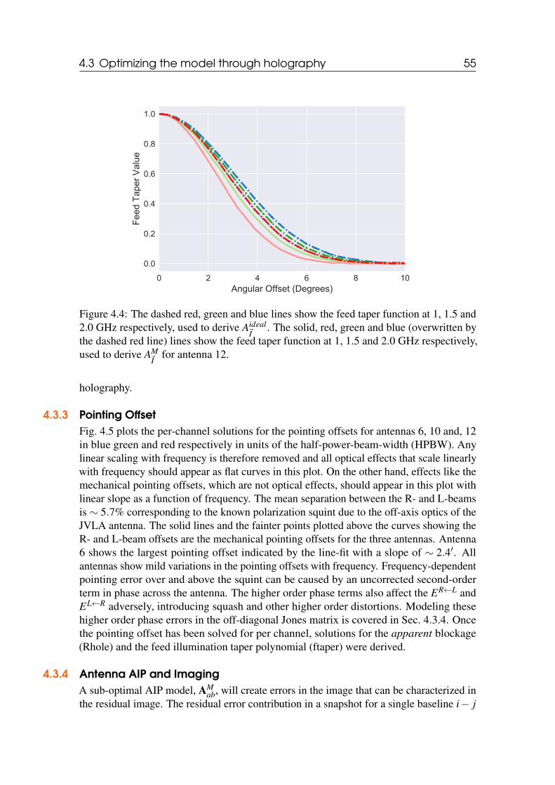
4.3 Optimizing the model through holography 55
0 2 4 6 8 10Angular Offset (Degrees)
0.0
0.2
0.4
0.6
0.8
1.0
Feed
Tap
er Value
Figure 4.4: The dashed red, green and blue lines show the feed taper function at 1, 1.5 and2.0 GHz respectively, used to derive Aideal
~I. The solid, red, green and blue (overwritten by
the dashed red line) lines show the feed taper function at 1, 1.5 and 2.0 GHz respectively,used to derive AM
~Ifor antenna 12.
holography.
4.3.3 Pointing OffsetFig. 4.5 plots the per-channel solutions for the pointing offsets for antennas 6, 10 and, 12in blue green and red respectively in units of the half-power-beam-width (HPBW). Anylinear scaling with frequency is therefore removed and all optical effects that scale linearlywith frequency should appear as flat curves in this plot. On the other hand, effects like themechanical pointing offsets, which are not optical effects, should appear in this plot withlinear slope as a function of frequency. The mean separation between the R- and L-beamsis ∼ 5.7% corresponding to the known polarization squint due to the off-axis optics of theJVLA antenna. The solid lines and the fainter points plotted above the curves showing theR- and L-beam offsets are the mechanical pointing offsets for the three antennas. Antenna6 shows the largest pointing offset indicated by the line-fit with a slope of ∼ 2.4′. Allantennas show mild variations in the pointing offsets with frequency. Frequency-dependentpointing error over and above the squint can be caused by an uncorrected second-orderterm in phase across the antenna. The higher order phase terms also affect the ER←L andEL←R adversely, introducing squash and other higher order distortions. Modeling thesehigher order phase errors in the off-diagonal Jones matrix is covered in Sec. 4.3.4. Oncethe pointing offset has been solved for per channel, solutions for the apparent blockage(Rhole) and the feed illumination taper polynomial (ftaper) were derived.
4.3.4 Antenna AIP and ImagingA sub-optimal AIP model, AM
ab, will create errors in the image that can be characterized inthe residual image. The residual error contribution in a snapshot for a single baseline i− j
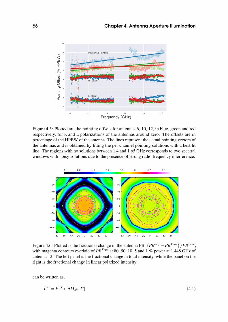
56 Chapter 4. Antenna Aperture Illumination
1.0 1.2 1.4 1.6 1.8 2.0
Frequency (GHz)
(4
(2
0
2
4
6
8
10
P inting Offset (%
HPBW)
R - Beam
L - Beam
Mechanical Pointing
Figure 4.5: Plotted are the pointing offsets for antennas 6, 10, 12, in blue, green and redrespectively, for R and L polarizations of the antennas around zero. The offsets are inpercentage of the HPBW of the antenna. The lines represent the actual pointing vectors ofthe antennas and is obtained by fitting the per channel pointing solutions with a best fitline. The regions with no solutions between 1.4 and 1.65 GHz corresponds to two spectralwindows with noisy solutions due to the presence of strong radio frequency interference.
Figure 4.6: Plotted is the fractional change in the antenna PB,(PBde f −PBTrue)/PBTrue,
with magenta contours overlaid of PBTrue at 80, 50, 10, 5 and 1 % power at 1.448 GHz ofantenna 12. The left panel is the fractional change in total intensity, while the panel on theright is the fractional change in linear polarized intensity
can be written as,
Ires = Ips f ? [∆Mab · I] (4.1)
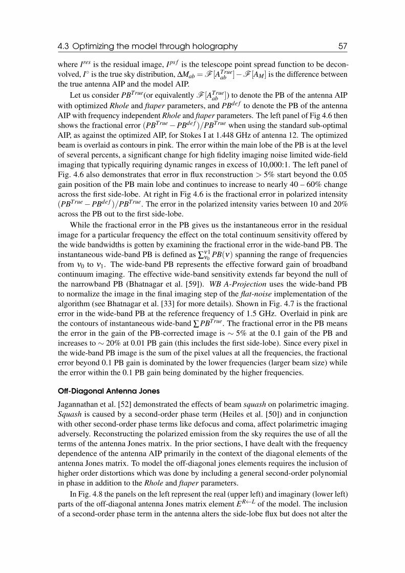
4.3 Optimizing the model through holography 57
where Ires is the residual image, Ips f is the telescope point spread function to be decon-volved, I is the true sky distribution, ∆Mab =F [ATrue
ab ]−F [AM] is the difference betweenthe true antenna AIP and the model AIP.
Let us consider PBTrue(or equivalently F [ATrueab ]) to denote the PB of the antenna AIP
with optimized Rhole and ftaper parameters, and PBde f to denote the PB of the antennaAIP with frequency independent Rhole and ftaper parameters. The left panel of Fig 4.6 thenshows the fractional error (PBTrue−PBde f )/PBTrue when using the standard sub-optimalAIP, as against the optimized AIP, for Stokes I at 1.448 GHz of antenna 12. The optimizedbeam is overlaid as contours in pink. The error within the main lobe of the PB is at the levelof several percents, a significant change for high fidelity imaging noise limited wide-fieldimaging that typically requiring dynamic ranges in excess of 10,000:1. The left panel ofFig. 4.6 also demonstrates that error in flux reconstruction > 5% start beyond the 0.05gain position of the PB main lobe and continues to increase to nearly 40 – 60% changeacross the first side-lobe. At right in Fig 4.6 is the fractional error in polarized intensity(PBTrue−PBde f )/PBTrue. The error in the polarized intensity varies between 10 and 20%across the PB out to the first side-lobe.
While the fractional error in the PB gives us the instantaneous error in the residualimage for a particular frequency the effect on the total continuum sensitivity offered bythe wide bandwidths is gotten by examining the fractional error in the wide-band PB. Theinstantaneous wide-band PB is defined as ∑
ν1ν0
PB(ν) spanning the range of frequenciesfrom ν0 to ν1. The wide-band PB represents the effective forward gain of broadbandcontinuum imaging. The effective wide-band sensitivity extends far beyond the null ofthe narrowband PB (Bhatnagar et al. [59]). WB A-Projection uses the wide-band PBto normalize the image in the final imaging step of the flat-noise implementation of thealgorithm (see Bhatnagar et al. [33] for more details). Shown in Fig. 4.7 is the fractionalerror in the wide-band PB at the reference frequency of 1.5 GHz. Overlaid in pink arethe contours of instantaneous wide-band ∑PBTrue. The fractional error in the PB meansthe error in the gain of the PB-corrected image is ∼ 5% at the 0.1 gain of the PB andincreases to ∼ 20% at 0.01 PB gain (this includes the first side-lobe). Since every pixel inthe wide-band PB image is the sum of the pixel values at all the frequencies, the fractionalerror beyond 0.1 PB gain is dominated by the lower frequencies (larger beam size) whilethe error within the 0.1 PB gain being dominated by the higher frequencies.
Off-Diagonal Antenna Jones
Jagannathan et al. [52] demonstrated the effects of beam squash on polarimetric imaging.Squash is caused by a second-order phase term (Heiles et al. [50]) and in conjunctionwith other second-order phase terms like defocus and coma, affect polarimetric imagingadversely. Reconstructing the polarized emission from the sky requires the use of all theterms of the antenna Jones matrix. In the prior sections, I have dealt with the frequencydependence of the antenna AIP primarily in the context of the diagonal elements of theantenna Jones matrix. To model the off-diagonal jones elements requires the inclusion ofhigher order distortions which was done by including a general second-order polynomialin phase in addition to the Rhole and ftaper parameters.
In Fig. 4.8 the panels on the left represent the real (upper left) and imaginary (lower left)parts of the off-diagonal antenna Jones matrix element ER←L of the model. The inclusionof a second-order phase term in the antenna alters the side-lobe flux but does not alter the
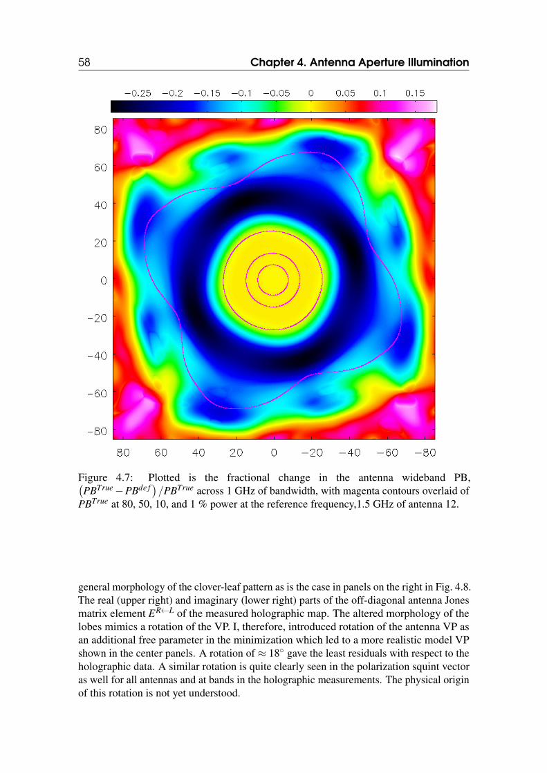
58 Chapter 4. Antenna Aperture Illumination
Figure 4.7: Plotted is the fractional change in the antenna wideband PB,(PBTrue−PBde f )/PBTrue across 1 GHz of bandwidth, with magenta contours overlaid of
PBTrue at 80, 50, 10, and 1 % power at the reference frequency,1.5 GHz of antenna 12.
general morphology of the clover-leaf pattern as is the case in panels on the right in Fig. 4.8.The real (upper right) and imaginary (lower right) parts of the off-diagonal antenna Jonesmatrix element ER←L of the measured holographic map. The altered morphology of thelobes mimics a rotation of the VP. I, therefore, introduced rotation of the antenna VP asan additional free parameter in the minimization which led to a more realistic model VPshown in the center panels. A rotation of ≈ 18 gave the least residuals with respect to theholographic data. A similar rotation is quite clearly seen in the polarization squint vectoras well for all antennas and at bands in the holographic measurements. The physical originof this rotation is not yet understood.
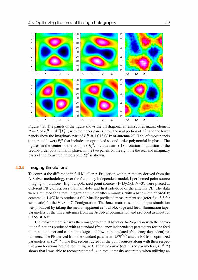
4.3 Optimizing the model through holography 59
Figure 4.8: The panels of the figure shows the off diagonal antenna Jones matrix elementR← L of EM
i = F †[AMi ], with the upper panels show the real portion of EM
i and the lowerpanels show the imaginary part of EM
i at 1.013 GHz of antenna 27. The left most panels(upper and lower) EM
i that includes an optimized second-order polynomial in phase. Thefigures in the center of the complex EM
i , includes an ≈ 18 rotation in addition to thesecond-order polynomial in phase. In the two panels on the right the the real and imaginaryparts of the measured holographic EM
i is shown.
4.3.5 Imaging SimulationsTo contrast the difference in full Mueller A-Projection with parameters derived from theA-Solver methodology over the frequency independent model, I performed point sourceimaging simulations. Eight unpolarized point sources (I=1Jy,Q,U,V=0), were placed atdifferent PB gains across the main-lobe and first side-lobe of the antenna PB. The datawere simulated for a total integration time of fifteen minutes, with a bandwidth of 64MHzcentered at 1.4GHz to produce a full Mueller predicted measurement set (refer fig . 3.3 forschematic) for the VLA in C-Configuration. The Jones matrix used in the input simulationwas produced by taking the median apparent central blockage and feed illumination taperparameters of the three antennas from the A-Solver optimization and provided as input forCASSBEAM.
The measurement set was then imaged with full Mueller A-Projection with the convo-lution functions produced with a) standard (frequency independent) parameters for the feedillumination taper and central blockage, and b)with the updated (frequency-dependent) pa-rameters. The PB derived from the standard parameters (PBde f ) and the PB from optimizedparameters as PBTrue. The flux reconstructed for the point sources along with their respec-tive gain locations are plotted in Fig. 4.9. The blue curve (optimized parameters, PBTrue)shows that I was able to reconstruct the flux in total intensity accurately when utilizing an
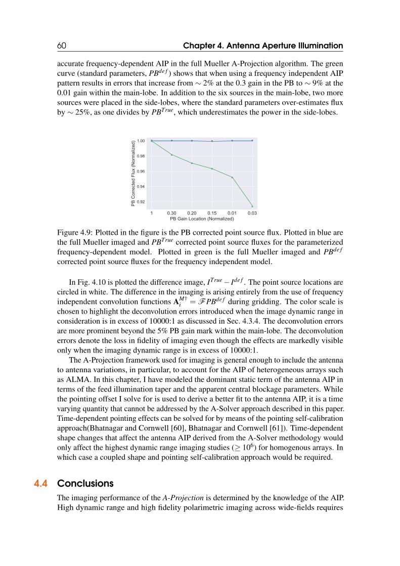
60 Chapter 4. Antenna Aperture Illumination
accurate frequency-dependent AIP in the full Mueller A-Projection algorithm. The greencurve (standard parameters, PBde f ) shows that when using a frequency independent AIPpattern results in errors that increase from ∼ 2% at the 0.3 gain in the PB to ∼ 9% at the0.01 gain within the main-lobe. In addition to the six sources in the main-lobe, two moresources were placed in the side-lobes, where the standard parameters over-estimates fluxby ∼ 25%, as one divides by PBTrue, which underestimates the power in the side-lobes.
1 0.30 0.20 0.15 0.01 0.03PB Gain Location (Normalized)
0.92
0.94
0.96
0.98
1.00
PB Corrected
Flux (N
ormalized
)
Figure 4.9: Plotted in the figure is the PB corrected point source flux. Plotted in blue arethe full Mueller imaged and PBTrue corrected point source fluxes for the parameterizedfrequency-dependent model. Plotted in green is the full Mueller imaged and PBde f
corrected point source fluxes for the frequency independent model.
In Fig. 4.10 is plotted the difference image, ITrue− Ide f . The point source locations arecircled in white. The difference in the imaging is arising entirely from the use of frequencyindependent convolution functions AM†
i = FPBde f during gridding. The color scale ischosen to highlight the deconvolution errors introduced when the image dynamic range inconsideration is in excess of 10000:1 as discussed in Sec. 4.3.4. The deconvolution errorsare more prominent beyond the 5% PB gain mark within the main-lobe. The deconvolutionerrors denote the loss in fidelity of imaging even though the effects are markedly visibleonly when the imaging dynamic range is in excess of 10000:1.
The A-Projection framework used for imaging is general enough to include the antennato antenna variations, in particular, to account for the AIP of heterogeneous arrays suchas ALMA. In this chapter, I have modeled the dominant static term of the antenna AIP interms of the feed illumination taper and the apparent central blockage parameters. Whilethe pointing offset I solve for is used to derive a better fit to the antenna AIP, it is a timevarying quantity that cannot be addressed by the A-Solver approach described in this paper.Time-dependent pointing effects can be solved for by means of the pointing self-calibrationapproach(Bhatnagar and Cornwell [60], Bhatnagar and Cornwell [61]). Time-dependentshape changes that affect the antenna AIP derived from the A-Solver methodology wouldonly affect the highest dynamic range imaging studies (≥ 106) for homogenous arrays. Inwhich case a coupled shape and pointing self-calibration approach would be required.
4.4 ConclusionsThe imaging performance of the A-Projection is determined by the knowledge of the AIP.High dynamic range and high fidelity polarimetric imaging across wide-fields requires
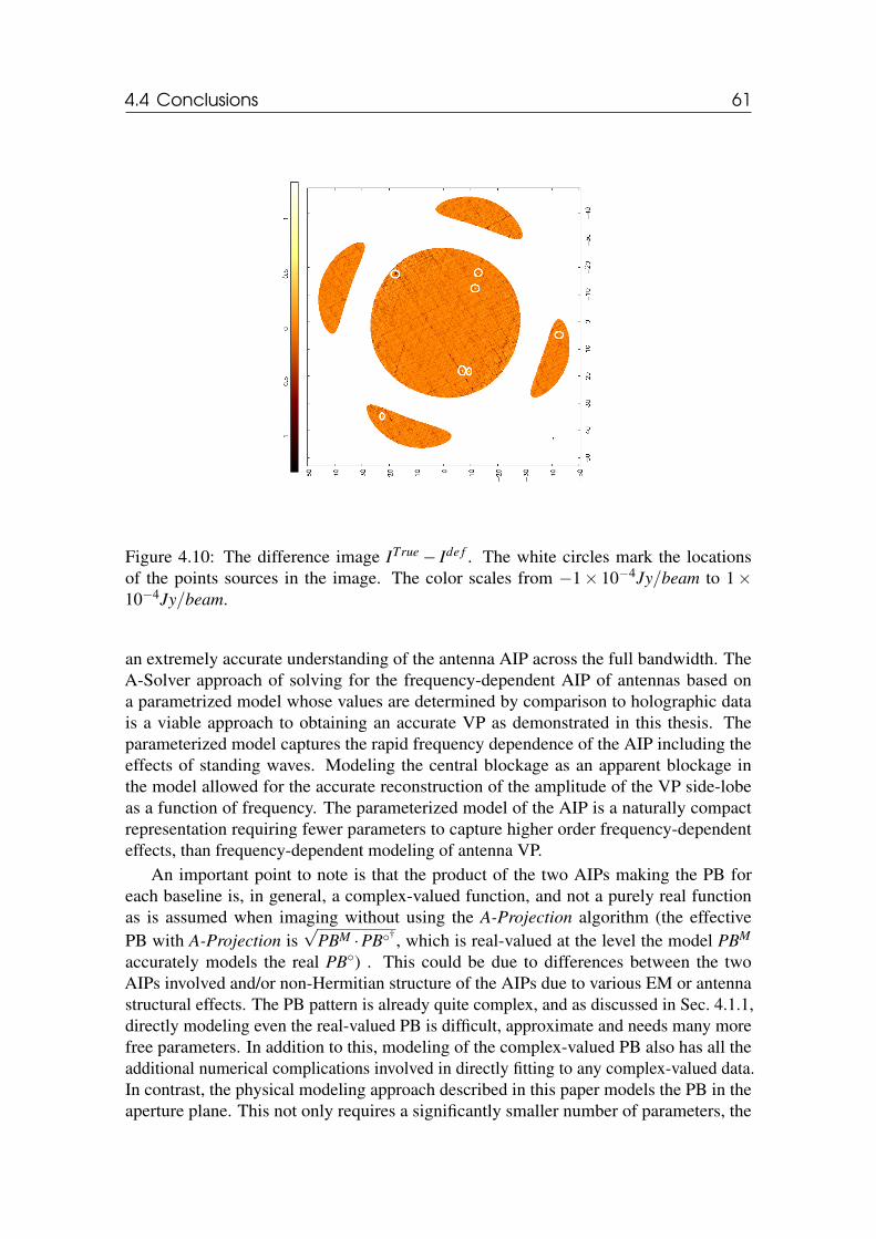
4.4 Conclusions 61
Figure 4.10: The difference image ITrue− Ide f . The white circles mark the locationsof the points sources in the image. The color scales from −1× 10⁻⁴Jy/beam to 1×10⁻⁴Jy/beam.
an extremely accurate understanding of the antenna AIP across the full bandwidth. TheA-Solver approach of solving for the frequency-dependent AIP of antennas based ona parametrized model whose values are determined by comparison to holographic datais a viable approach to obtaining an accurate VP as demonstrated in this thesis. Theparameterized model captures the rapid frequency dependence of the AIP including theeffects of standing waves. Modeling the central blockage as an apparent blockage inthe model allowed for the accurate reconstruction of the amplitude of the VP side-lobeas a function of frequency. The parameterized model of the AIP is a naturally compactrepresentation requiring fewer parameters to capture higher order frequency-dependenteffects, than frequency-dependent modeling of antenna VP.
An important point to note is that the product of the two AIPs making the PB foreach baseline is, in general, a complex-valued function, and not a purely real functionas is assumed when imaging without using the A-Projection algorithm (the effectivePB with A-Projection is
√PBM ·PB† , which is real-valued at the level the model PBM
accurately models the real PB) . This could be due to differences between the twoAIPs involved and/or non-Hermitian structure of the AIPs due to various EM or antennastructural effects. The PB pattern is already quite complex, and as discussed in Sec. 4.1.1,directly modeling even the real-valued PB is difficult, approximate and needs many morefree parameters. In addition to this, modeling of the complex-valued PB also has all theadditional numerical complications involved in directly fitting to any complex-valued data.In contrast, the physical modeling approach described in this paper models the PB in theaperture plane. This not only requires a significantly smaller number of parameters, the

62 Chapter 4. Antenna Aperture Illumination
parameters themselves are real-valued describing the physics of the optics (here, via theantenna structural parameters). The fitting procedure, therefore, deals with real-valuedparameters. This has significant numerical advantages, and computational advantages inthe production of parameterized convolution functions for a given frequency.
5. Full Mueller A-Projection
In chapter 2, I have established that there exist a class of algorithms that can account forDD effects during convolutional gridding. In this chapter, I will also outline the algorithmicdetails of the Full Mueller A-Projection (FM-AWP) algorithm. Further, I will apply thealgorithm to simulated data and demonstrate imaging results in the case of representativepoint sources spread across the antenna PB and a radio field. In both of these cases, thefocus is on the comparison of imaging fidelity with FM-AWP as against standard imaging.Finally, I will apply the algorithm to VLA test data at L-Band and discuss the results.
5.1 A-Projection Algorithm
In chapter 2 I briefly introduced the A-Projection algorithm which corrects for the antennaAIP during the imaging major cycle as a convolutional gridding correction. The correctionis carried out in two stages during the imaging major cycle. While the algorithm allowsfor different kinds of image normalization, I discuss the "flat noise" case of normalizationwhich allows for the minor cycle algorithms to carry out deconvolution on an image withuniform noise across the entirety of the image. The algorithm presented in Alg. 1 is thegeneral wide-band FM-AWP form of the algorithm. In the forward step described below,for the narrowband case, the conjugate frequency reduces to the true frequency of the databeing gridded, i.e. ν∗ = ν .
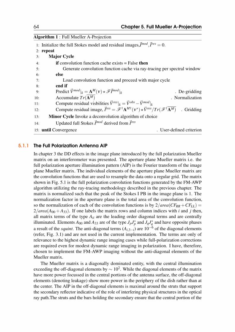
64 Chapter 5. Full Mueller A-Projection
Algorithm 1 : Full Mueller A-Projection
1: Initialize the full Stokes model and residual images,~Imod,~Ires = 0.2: repeat3: Major Cycle4: if convolution function cache exists = False then5: Generate convolution function cache via ray-tracing per spectral window6: else7: Load convolution function and proceed with major cycle8: end if9: Predict ~V mod|k = AM(ν)?F~Imod|k . De-gridding
10: Accumulate Tr(AM) . Normalization11: Compute residual visbilities ~V res|k =~V obs−~V mod|k12: Compute residual image,~Ires = F †AM†(ν∗)?~V res/Tr(F †AM) . Gridding13: Minor Cycle Invoke a deconvolution algorithm of choice14: Updated full Stokes~Imod derived from~Ires
15: until Convergence . User-defined criterion
5.1.1 The Full Polarization Antenna AIP
In chapter 3 the DD effects in the image plane introduced by the full polarization Muellermatrix on an interferometer was presented. The aperture plane Mueller matrix i.e. thefull polarization aperture illumination pattern (AIP) is the Fourier transform of the imageplane Mueller matrix. The individual elements of the aperture plane Mueller matrix arethe convolution functions that are used to resample the data onto a regular grid. The matrixshown in Fig. 5.1 is the full polarization convolution functions generated by the FM-AWPalgorithm utilizing the ray-tracing methodology described in the previous chapter. Thematrix is normalized such that the peak of the Stokes I PB in the image plane is 1. Thenormalization factor in the aperture plane is the total area of the convolution function,so the normalization of each of the convolution functions is by 2/area(CFRR +CFLL) =2/area(A00 +A33). If one labels the matrix rows and column indices with i and j then,all matrix terms of the type Aii are the leading order diagonal terms and are centrallyilluminated. Elements A00 and A33 are of the type JpJ∗p and JqJ∗q and have opposite phasesa result of the squint. The anti-diagonal terms (Ai,3−i) are 10−6 of the diagonal elements(refer, Fig. 3.1) and are not used in the current implementation. The terms are only ofrelevance to the highest dynamic range imaging cases while full-polarization correctionsare required even for modest dynamic range imaging in polarization. I have, therefore,chosen to implement the FM-AWP imaging without the anti-diagonal elements of theMueller matrix.
The Mueller matrix is a diagonally dominated entity, with the central illuminationexceeding the off-diagonal elements by ∼ 102. While the diagonal elements of the matrixhave more power focussed in the central portions of the antenna surface, the off-diagonalelements (denoting leakage) show more power in the periphery of the dish rather than atthe center. The AIP in the off-diagonal elements is maximal around the struts that supportthe secondary reflector indicative of the role of interfering physical structures in the opticalray path.The struts and the bars holding the secondary ensure that the central portion of the
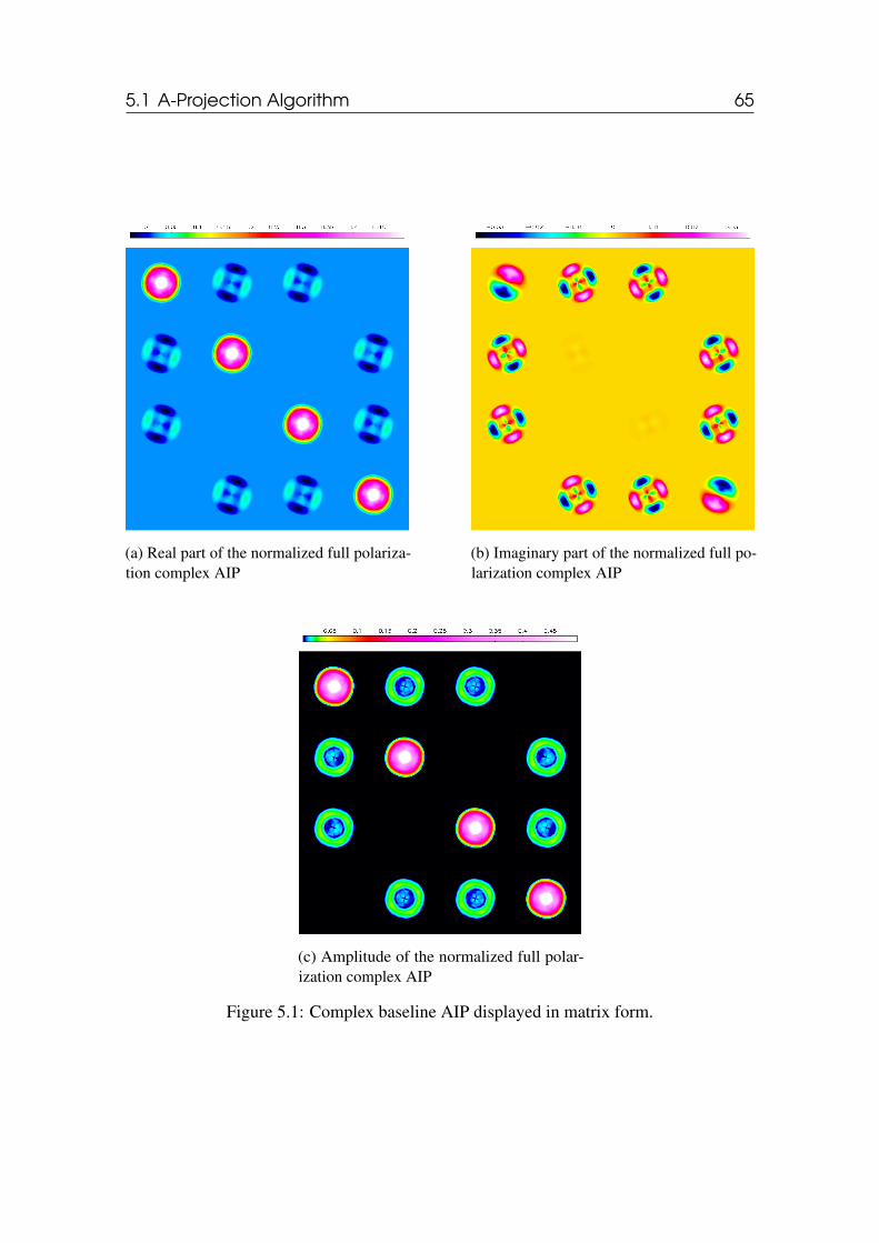
5.1 A-Projection Algorithm 65
(a) Real part of the normalized full polariza-tion complex AIP
(b) Imaginary part of the normalized full po-larization complex AIP
(c) Amplitude of the normalized full polar-ization complex AIP
Figure 5.1: Complex baseline AIP displayed in matrix form.
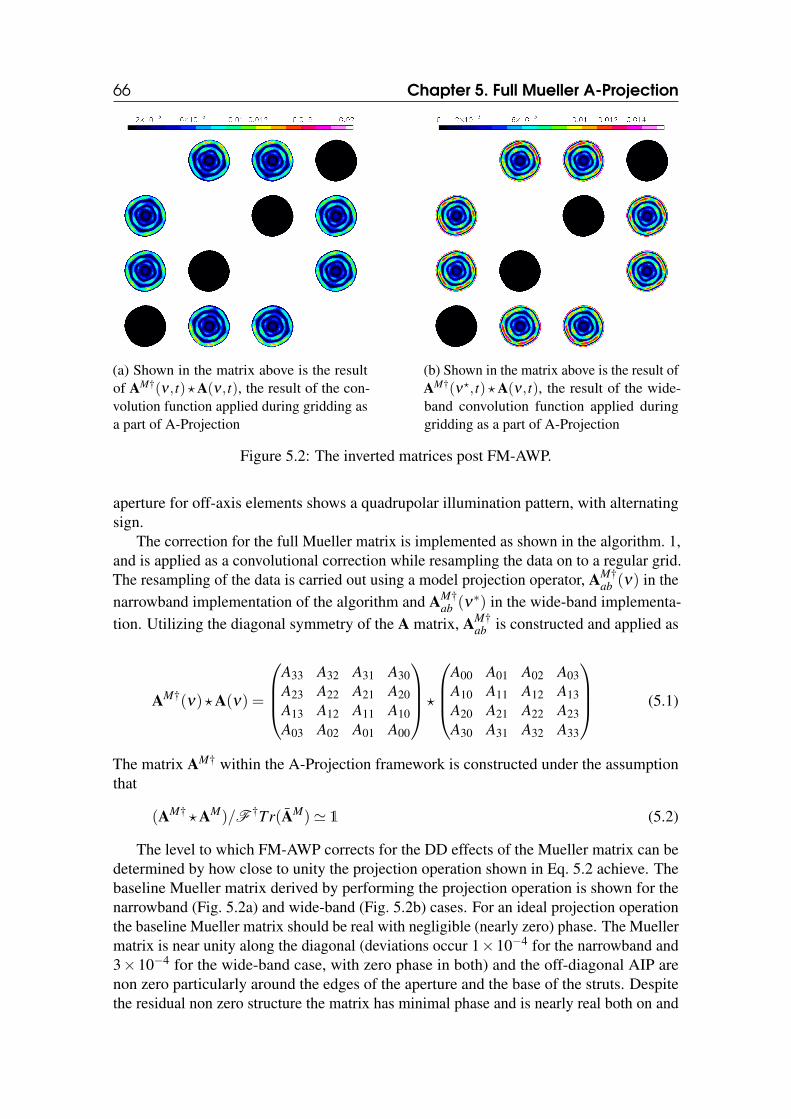
66 Chapter 5. Full Mueller A-Projection
(a) Shown in the matrix above is the resultof AM†(ν , t) ?A(ν , t), the result of the con-volution function applied during gridding asa part of A-Projection
(b) Shown in the matrix above is the result ofAM†(ν?, t) ?A(ν , t), the result of the wide-band convolution function applied duringgridding as a part of A-Projection
Figure 5.2: The inverted matrices post FM-AWP.
aperture for off-axis elements shows a quadrupolar illumination pattern, with alternatingsign.
The correction for the full Mueller matrix is implemented as shown in the algorithm. 1,and is applied as a convolutional correction while resampling the data on to a regular grid.The resampling of the data is carried out using a model projection operator, AM†
ab (ν) in thenarrowband implementation of the algorithm and AM†
ab (ν∗) in the wide-band implementa-tion. Utilizing the diagonal symmetry of the A matrix, AM†
ab is constructed and applied as
AM†(ν)?A(ν) =
A33 A32 A31 A30A23 A22 A21 A20A13 A12 A11 A10A03 A02 A01 A00
?
A00 A01 A02 A03A10 A11 A12 A13A20 A21 A22 A23A30 A31 A32 A33
(5.1)
The matrix AM† within the A-Projection framework is constructed under the assumptionthat
(AM† ?AM)/F †Tr(AM)' 1 (5.2)
The level to which FM-AWP corrects for the DD effects of the Mueller matrix can bedetermined by how close to unity the projection operation shown in Eq. 5.2 achieve. Thebaseline Mueller matrix derived by performing the projection operation is shown for thenarrowband (Fig. 5.2a) and wide-band (Fig. 5.2b) cases. For an ideal projection operationthe baseline Mueller matrix should be real with negligible (nearly zero) phase. The Muellermatrix is near unity along the diagonal (deviations occur 1×10⁻⁴ for the narrowband and3×10−4 for the wide-band case, with zero phase in both) and the off-diagonal AIP arenon zero particularly around the edges of the aperture and the base of the struts. Despitethe residual non zero structure the matrix has minimal phase and is nearly real both on and
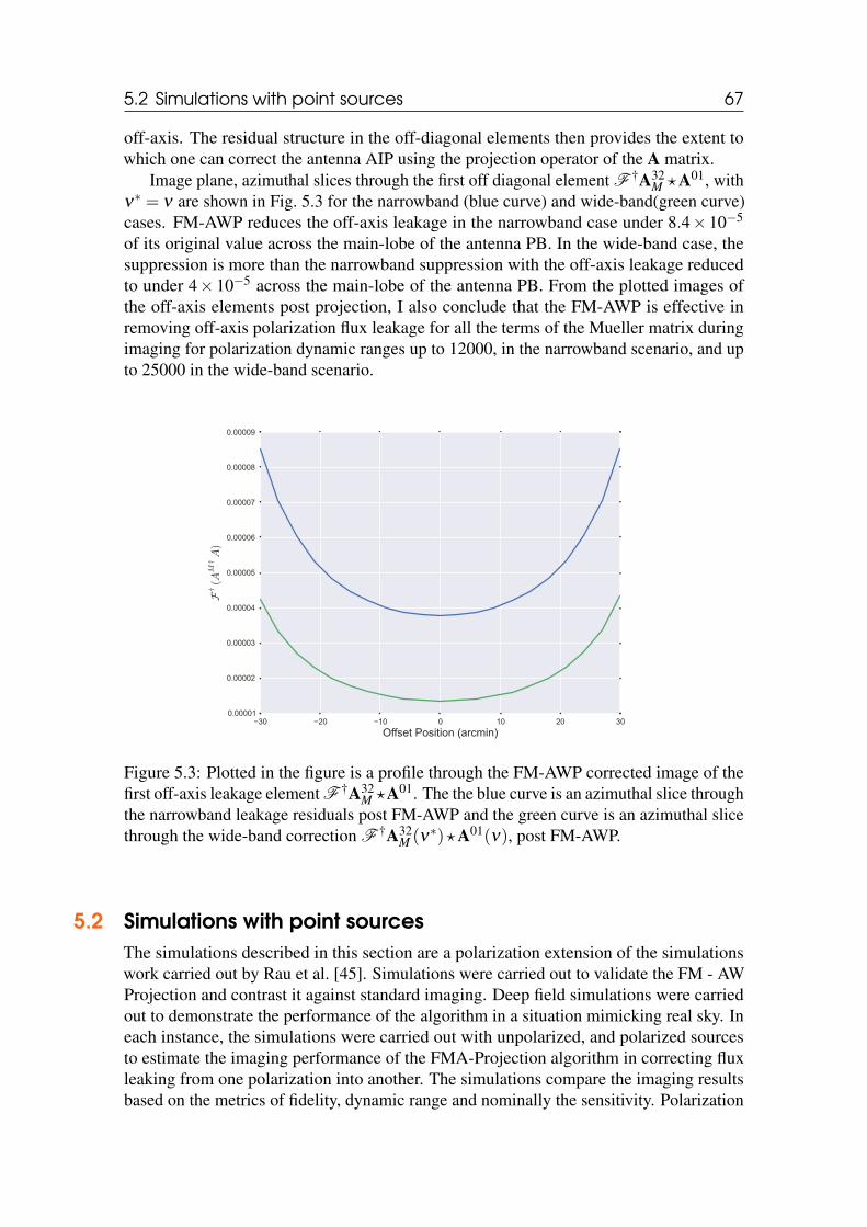
5.2 Simulations with point sources 67
off-axis. The residual structure in the off-diagonal elements then provides the extent towhich one can correct the antenna AIP using the projection operator of the A matrix.
Image plane, azimuthal slices through the first off diagonal element F †A32M ?A01, with
ν∗ = ν are shown in Fig. 5.3 for the narrowband (blue curve) and wide-band(green curve)cases. FM-AWP reduces the off-axis leakage in the narrowband case under 8.4×10⁻⁵
of its original value across the main-lobe of the antenna PB. In the wide-band case, thesuppression is more than the narrowband suppression with the off-axis leakage reducedto under 4× 10⁻⁵ across the main-lobe of the antenna PB. From the plotted images ofthe off-axis elements post projection, I also conclude that the FM-AWP is effective inremoving off-axis polarization flux leakage for all the terms of the Mueller matrix duringimaging for polarization dynamic ranges up to 12000, in the narrowband scenario, and upto 25000 in the wide-band scenario.
−30 −20 −10 0 10 20 30Offset Position (arcmin)
0.00001
0.00002
0.00003
0.00004
0.00005
0.00006
0.00007
0.00008
0.00009
F†(AM
†A)
Figure 5.3: Plotted in the figure is a profile through the FM-AWP corrected image of thefirst off-axis leakage element F †A32
M ?A01. The the blue curve is an azimuthal slice throughthe narrowband leakage residuals post FM-AWP and the green curve is an azimuthal slicethrough the wide-band correction F †A32
M (ν∗)?A01(ν), post FM-AWP.
5.2 Simulations with point sourcesThe simulations described in this section are a polarization extension of the simulationswork carried out by Rau et al. [45]. Simulations were carried out to validate the FM - AWProjection and contrast it against standard imaging. Deep field simulations were carriedout to demonstrate the performance of the algorithm in a situation mimicking real sky. Ineach instance, the simulations were carried out with unpolarized, and polarized sourcesto estimate the imaging performance of the FMA-Projection algorithm in correcting fluxleaking from one polarization into another. The simulations compare the imaging resultsbased on the metrics of fidelity, dynamic range and nominally the sensitivity. Polarization
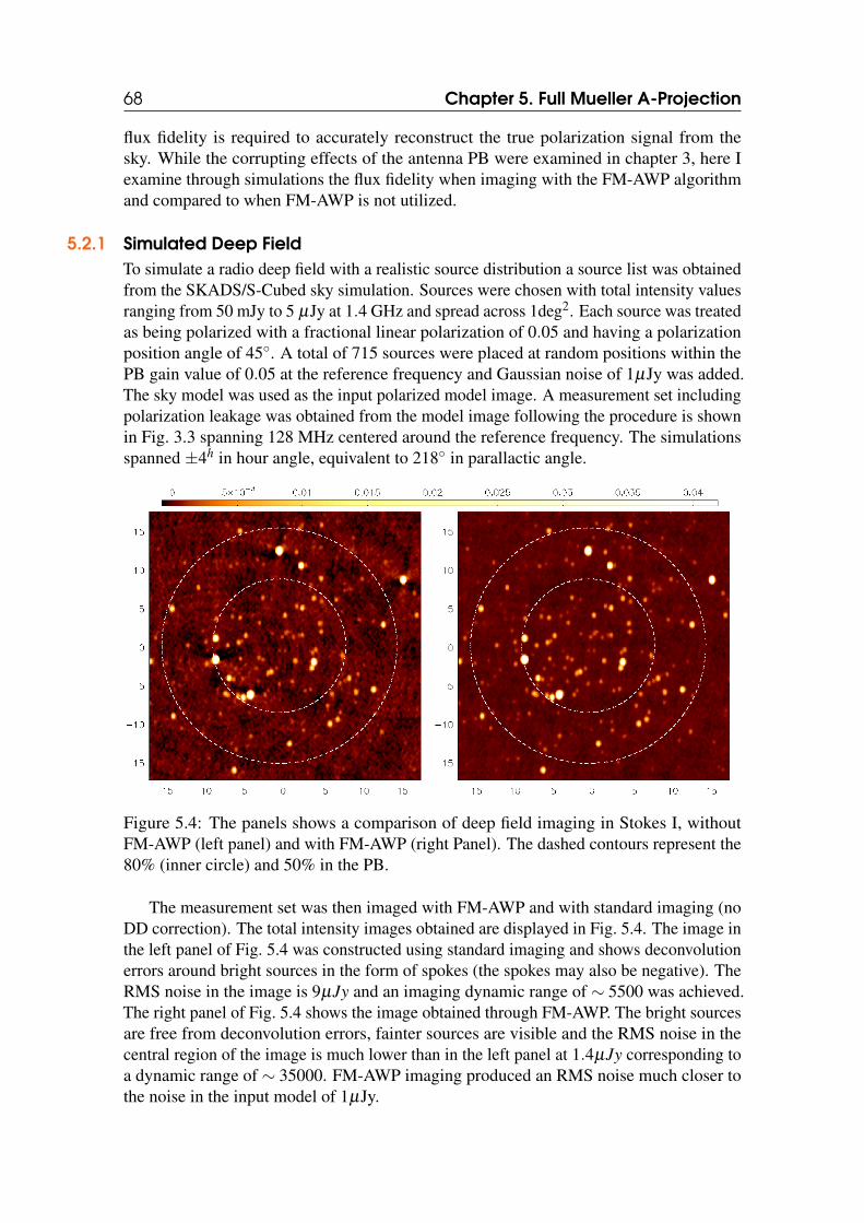
68 Chapter 5. Full Mueller A-Projection
flux fidelity is required to accurately reconstruct the true polarization signal from thesky. While the corrupting effects of the antenna PB were examined in chapter 3, here Iexamine through simulations the flux fidelity when imaging with the FM-AWP algorithmand compared to when FM-AWP is not utilized.
5.2.1 Simulated Deep FieldTo simulate a radio deep field with a realistic source distribution a source list was obtainedfrom the SKADS/S-Cubed sky simulation. Sources were chosen with total intensity valuesranging from 50 mJy to 5 µJy at 1.4 GHz and spread across 1deg2. Each source was treatedas being polarized with a fractional linear polarization of 0.05 and having a polarizationposition angle of 45. A total of 715 sources were placed at random positions within thePB gain value of 0.05 at the reference frequency and Gaussian noise of 1µJy was added.The sky model was used as the input polarized model image. A measurement set includingpolarization leakage was obtained from the model image following the procedure is shownin Fig. 3.3 spanning 128 MHz centered around the reference frequency. The simulationsspanned ±4h in hour angle, equivalent to 218 in parallactic angle.
Figure 5.4: The panels shows a comparison of deep field imaging in Stokes I, withoutFM-AWP (left panel) and with FM-AWP (right Panel). The dashed contours represent the80% (inner circle) and 50% in the PB.
The measurement set was then imaged with FM-AWP and with standard imaging (noDD correction). The total intensity images obtained are displayed in Fig. 5.4. The image inthe left panel of Fig. 5.4 was constructed using standard imaging and shows deconvolutionerrors around bright sources in the form of spokes (the spokes may also be negative). TheRMS noise in the image is 9µJy and an imaging dynamic range of ∼ 5500 was achieved.The right panel of Fig. 5.4 shows the image obtained through FM-AWP. The bright sourcesare free from deconvolution errors, fainter sources are visible and the RMS noise in thecentral region of the image is much lower than in the left panel at 1.4µJy corresponding toa dynamic range of ∼ 35000. FM-AWP imaging produced an RMS noise much closer tothe noise in the input model of 1µJy.
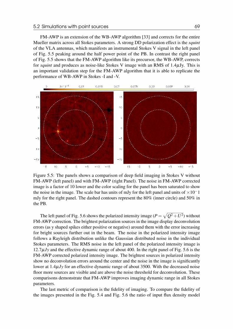
5.2 Simulations with point sources 69
FM-AWP is an extension of the WB-AWP algorithm [33] and corrects for the entireMueller matrix across all Stokes parameters. A strong DD polarization effect is the squintof the VLA antennas, which manifests an instrumental Stokes V signal in the left panelof Fig. 5.5 peaking around the half power point of the PB. In contrast the right panelof Fig. 5.5 shows that the FM-AWP algorithm like its precursor, the WB-AWP, correctsfor squint and produces as noise-like Stokes V image with an RMS of 1.4µJy. This isan important validation step for the FM-AWP algorithm that it is able to replicate theperformance of WB-AWP in Stokes -I and -V.
Figure 5.5: The panels shows a comparison of deep field imaging in Stokes V withoutFM-AWP (left panel) and with FM-AWP (right Panel). The noise in FM-AWP correctedimage is a factor of 10 lower and the color scaling for the panel has been saturated to showthe noise in the image. The scale bar has units of mJy for the left panel and units of ×10−1mJy for the right panel. The dashed contours represent the 80% (inner circle) and 50% inthe PB.
The left panel of Fig. 5.6 shows the polarized intensity image (P =√
Q2 +U2) withoutFM-AWP correction. The brightest polarization sources in the image display deconvolutionerrors (as y shaped spikes either positive or negative) around them with the error increasingfor bright sources further out in the beam. The noise in the polarized intensity imagefollows a Rayleigh distribution unlike the Gaussian distributed noise in the individualStokes parameters. The RMS noise in the left panel of the polarized intensity image is12.7µJy and the effective dynamic range of about 400. In the right panel of Fig. 5.6 is theFM-AWP corrected polarized intensity image. The brightest sources in polarized intensityshow no deconvolution errors around the center and the noise in the image is significantlylower at 1.4µJy for an effective dynamic range of about 3500. With the decreased noisefloor more sources are visible and are above the noise threshold for deconvolution. Thesecomparisons demonstrate that FM-AWP improves imaging dynamic range in all Stokesparameters.
The last metric of comparison is the fidelity of imaging. To compare the fidelity ofthe images presented in the Fig. 5.4 and Fig. 5.6 the ratio of input flux density model
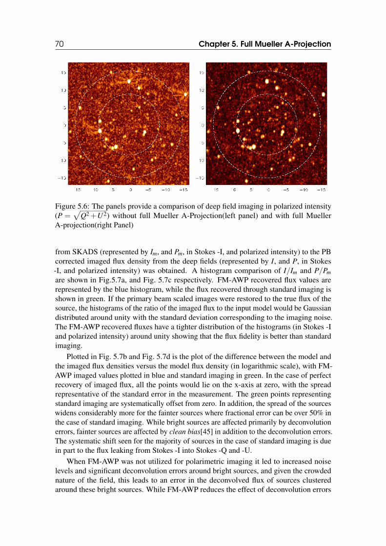
70 Chapter 5. Full Mueller A-Projection
Figure 5.6: The panels provide a comparison of deep field imaging in polarized intensity(P =
√Q2 +U2) without full Mueller A-Projection(left panel) and with full Mueller
A-projection(right Panel)
from SKADS (represented by Im, and Pm, in Stokes -I, and polarized intensity) to the PBcorrected imaged flux density from the deep fields (represented by I, and P, in Stokes-I, and polarized intensity) was obtained. A histogram comparison of I/Im and P/Pmare shown in Fig.5.7a, and Fig. 5.7c respectively. FM-AWP recovered flux values arerepresented by the blue histogram, while the flux recovered through standard imaging isshown in green. If the primary beam scaled images were restored to the true flux of thesource, the histograms of the ratio of the imaged flux to the input model would be Gaussiandistributed around unity with the standard deviation corresponding to the imaging noise.The FM-AWP recovered fluxes have a tighter distribution of the histograms (in Stokes -Iand polarized intensity) around unity showing that the flux fidelity is better than standardimaging.
Plotted in Fig. 5.7b and Fig. 5.7d is the plot of the difference between the model andthe imaged flux densities versus the model flux density (in logarithmic scale), with FM-AWP imaged values plotted in blue and standard imaging in green. In the case of perfectrecovery of imaged flux, all the points would lie on the x-axis at zero, with the spreadrepresentative of the standard error in the measurement. The green points representingstandard imaging are systematically offset from zero. In addition, the spread of the sourceswidens considerably more for the fainter sources where fractional error can be over 50% inthe case of standard imaging. While bright sources are affected primarily by deconvolutionerrors, fainter sources are affected by clean bias[45] in addition to the deconvolution errors.The systematic shift seen for the majority of sources in the case of standard imaging is duein part to the flux leaking from Stokes -I into Stokes -Q and -U.
When FM-AWP was not utilized for polarimetric imaging it led to increased noiselevels and significant deconvolution errors around bright sources, and given the crowdednature of the field, this leads to an error in the deconvolved flux of sources clusteredaround these bright sources. While FM-AWP reduces the effect of deconvolution errors
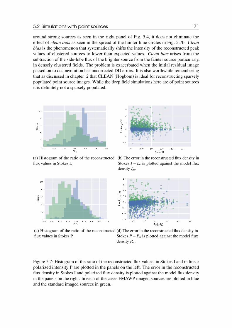
5.2 Simulations with point sources 71
around strong sources as seen in the right panel of Fig. 5.4, it does not eliminate theeffect of clean bias as seen in the spread of the fainter blue circles in Fig. 5.7b. Cleanbias is the phenomenon that systematically shifts the intensity of the reconstructed peakvalues of clustered sources to lower than expected values. Clean bias arises from thesubtraction of the side-lobe flux of the brighter source from the fainter source particularly,in densely clustered fields. The problem is exacerbated when the initial residual imagepassed on to deconvolution has uncorrected DD errors. It is also worthwhile rememberingthat as discussed in chapter 2 that CLEAN (Hogbom) is ideal for reconstructing sparselypopulated point source images. While the deep field simulations here are of point sourcesit is definitely not a sparsely populated.
(a) Histogram of the ratio of the reconstructedflux values in Stokes I.
(b) The error in the reconstructed flux density inStokes I− Im is plotted against the model fluxdensity Im.
(c) Histogram of the ratio of the reconstructedflux values in Stokes P.
(d) The error in the reconstructed flux density inStokes P−Pm is plotted against the model fluxdensity Pm.
Figure 5.7: Histogram of the ratio of the reconstructed flux values, in Stokes I and in linearpolarized intensity P are plotted in the panels on the left. The error in the reconstructedflux density in Stokes I and polarized flux density is plotted against the model flux densityin the panels on the right. In each of the cases FMAWP imaged sources are plotted in blueand the standard imaged sources in green.
72 Chapter 5. Full Mueller A-Projection
5.3 Full Mueller Imaging of Supernova Remnant G55.7+3.4G55.7+3.4 is a supernova remnant observed by the enhanced VLA [59], the data areavailable in the public domain. The observations were designed to produce an imagingtest dataset spanning 1−2 GHz with the supernova remnant occupying the entire PB ofthe telescope at 2 GHz. Being a complex extended source that is significantly affectedby DD effects across the band, it is an ideal reference source to test the new FM-AWPalgorithm. The data were taken on August 23rd , 2010 in D-configuration with the WIDARcorrelator. There were four non-working antennas which did not have the upgradedwide-band receivers at that time. Two primary flux calibrators 3C147 and 3C286, and asecondary phase calibrator J1925+2106 were observed. J1925+2106 was observed every30 minutes covering a wide array of parallactic angles over the 8-hour observation.
5.3.1 CalibrationThe data were flagged using auto-flagging algorithms implemented in CASA via theflagdata task and calibrated using the procedure outlined in the CASA guide1 to producethe bandpass and gain calibration tables. For wide-band polarization calibration, additionalcalibration steps are required. The model for the primary calibrator included was frequency-dependent (Perley and Butler [54]). 3C286 is linearly polarized (Perley and Butler [55])with a known partial polarization spectral index across the band, with an RM = 0 and apolarization position angle of 33 and hence is a primary polarization angle calibrator.The setjy task within CASA was used to set the flux density model in total intensity,utilizing the spectral index and curvature terms. The task is also capable of setting afrequency-dependent polynomial model in fractional polarization (ΠL) and polarizationposition angle (ψ) along with the source rotation measure (RM = 0). This was used to setthe flux density model of the polarization angle calibrator 3C286.
In addition to the total intensity calibration, polarization angle calibration on a perchannel basis was carried out using 3C286 as the reference source. The secondary phasecalibrator J1925+2106 was used to compute the polarization leakage with no constraintson the source polarization, using the Xf+QU mode in the polcal task in CASA. Thepolarization calibration along with the gain and bandpass calibration tables derived fromthe CASA guide was applied to the data. Spectral window 5 (centered at 1.576 GHz) wasnot used for calibration or imaging due to excessive RFI in this part of the frequency band.
5.3.2 Full Mueller ImagingThe data were imaged in all Stokes polarization using W-Projection (major cycle) andMT-MFS (minor cycle), a combination referred to here on as "standard imaging". Thedata were also imaged using FM-AWP (major cycle) and MT-MFS (minor cycle) in allStokes polarizations. In both imaging cases 64 w-planes and 2 nterms were used. Forthe FM-AWP imaging, convolution functions were generated and cached to disk to beused during gridding. For each of the 64 w-planes, 12 convolution functions (as shown inFig. 5.1 for w=0 are generated. One convolution function for each Mueller matrix elementbarring the 4 second-order elements) per Mueller matrix are generated, for a total of 768convolution functions that are cached on disk. During gridding in FM-AWP imaging the
1https://casaguides.nrao.edu/index.php/EVLA_Wide-Band_Wide-Field_Imaging:_G55.7_3.4-CASA4.4
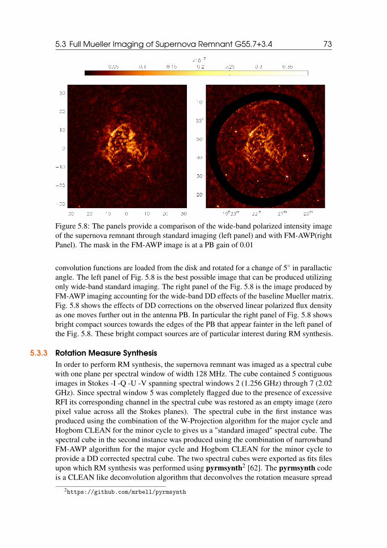
5.3 Full Mueller Imaging of Supernova Remnant G55.7+3.4 73
Figure 5.8: The panels provide a comparison of the wide-band polarized intensity imageof the supernova remnant through standard imaging (left panel) and with FM-AWP(rightPanel). The mask in the FM-AWP image is at a PB gain of 0.01
convolution functions are loaded from the disk and rotated for a change of 5 in parallacticangle. The left panel of Fig. 5.8 is the best possible image that can be produced utilizingonly wide-band standard imaging. The right panel of the Fig. 5.8 is the image produced byFM-AWP imaging accounting for the wide-band DD effects of the baseline Mueller matrix.Fig. 5.8 shows the effects of DD corrections on the observed linear polarized flux densityas one moves further out in the antenna PB. In particular the right panel of Fig. 5.8 showsbright compact sources towards the edges of the PB that appear fainter in the left panel ofthe Fig. 5.8. These bright compact sources are of particular interest during RM synthesis.
5.3.3 Rotation Measure SynthesisIn order to perform RM synthesis, the supernova remnant was imaged as a spectral cubewith one plane per spectral window of width 128 MHz. The cube contained 5 contiguousimages in Stokes -I -Q -U -V spanning spectral windows 2 (1.256 GHz) through 7 (2.02GHz). Since spectral window 5 was completely flagged due to the presence of excessiveRFI its corresponding channel in the spectral cube was restored as an empty image (zeropixel value across all the Stokes planes). The spectral cube in the first instance wasproduced using the combination of the W-Projection algorithm for the major cycle andHogbom CLEAN for the minor cycle to gives us a "standard imaged" spectral cube. Thespectral cube in the second instance was produced using the combination of narrowbandFM-AWP algorithm for the major cycle and Hogbom CLEAN for the minor cycle toprovide a DD corrected spectral cube. The two spectral cubes were exported as fits filesupon which RM synthesis was performed using pyrmsynth2 [62]. The pyrmsynth codeis a CLEAN like deconvolution algorithm that deconvolves the rotation measure spread
2https://github.com/mrbell/pyrmsynth
74 Chapter 5. Full Mueller A-Projection
function (RMSF) from the band-limited Faraday depth function (FDF). The band-limitedFDF as given by Eq. 3.5, is a function of the polarized intensity per channel Pi(λ
2), whereλ is the wavelength of the channel i. DD imaging corrections through FM-AWP alters thePi per channel for sources lying farther out in the antenna PB. Since the RMSF is nearlyidentical for the two spectral cubes (RMSF depends only on bandwidth and channelization)and has an HPBW of ≈ 130 rad/m2. So any difference in the derived Faraday depthfunction of the two channel cubes is a result of DD imaging corrections.
In chapter 3 I show that the Full Mueller Antenna PB needs to be accounted for inorder to allow unencumbered deconvolution of RMSF from the FDF. So any uncorrectedeffects in the antenna PB will result in deconvolution errors in Faraday space that increaseswith distance from the center of the PB. To quantify the deconvolution error introducedin the cleaned RM map, the pyrmsynth code was run on the image cubes produced withand without FM-AWP imaging. Since the sources in this field are fainter than the NVSSdetection threshold they do not have a prior RM value in [6]. However, the median RMderived from 60 of the nearest sources around the supernova remnant puts the median RMfor the galactic latitude (l = 55), and longitude (b = 3) at 110 rad/m2 3. In Fig. 5.9a thedeconvolved RM of the supernova remnant derived from FM-AWP corrected image hasa median RM of 125 rad/m2. Fig. 5.9b shows the difference in the RM obtained whenFaraday synthesis was performed on the image cube with and without FM-AWP. In regionsof high signal to noise, the deconvolution of the RMSF from the FDF is similar in bothinstances at the center of the PB.
For a closer examination of the FDF and the effect FM-AWP has on the data, threelines of sights across the Faraday depth cube are plotted in the Fig 5.10. Plotted in blueis the FDF derived from the FM-AWP corrected cube while plotted in green are the FDFderived from standard imaging. In Fig. 5.10a the data are derived from the central regionof the image around the 0.8 gain in the PB at the reference frequency 1.64 GHz, of diffuseextended emission in the supernova remnant. The plotted points differ from each otherin polarized intensity by about 5 % where the polarized intensity peaks at an FDF of 120rad/m2, in line with the median RM predicted by Taylor et al. [6]. The Fig. 5.10c containsa point source (brightest source in the map, J1920+2129 on the south eastern side of thesupernova remnant) located at a PB gain of 0.2 at the reference frequency of 1.64 GHz.The Pi contribution to the FDF in the case of FM-AWP is significantly different from thePi in the standard imaging cube. This difference in the FDF results in a shifted peak ofpolarized intensity in the FDF form 120 rad/m2 in the case of FM-AWP to ≈−180 rad/m2
for standard imaging, along with a 15% reduction in the peak polarized flux.
5.4 ConclusionsIn this chapter, I introduced the FM-AWP algorithm and demonstrated the existence ofthe inverse of the A matrix in both the case of narrowband and wide-band imaging cases.I have shown that the FM-AWP algorithm is capable of correcting for the effects of fullMueller matrix down to 8.4× 10⁻⁵ of the Stokes I flux in the main-lobe and the firstside-lobe in the narrowband case and 4× 10⁻⁵ of the Stokes I flux in the wide-bandcase. Through simulations of deep radio fields, I have demonstrated that the FM-AWP
3The median RM is a reasonable estimate of the expected RM in the galactic plane as the plasmas probedwould be galactic and lying at a similar depth in Faraday space
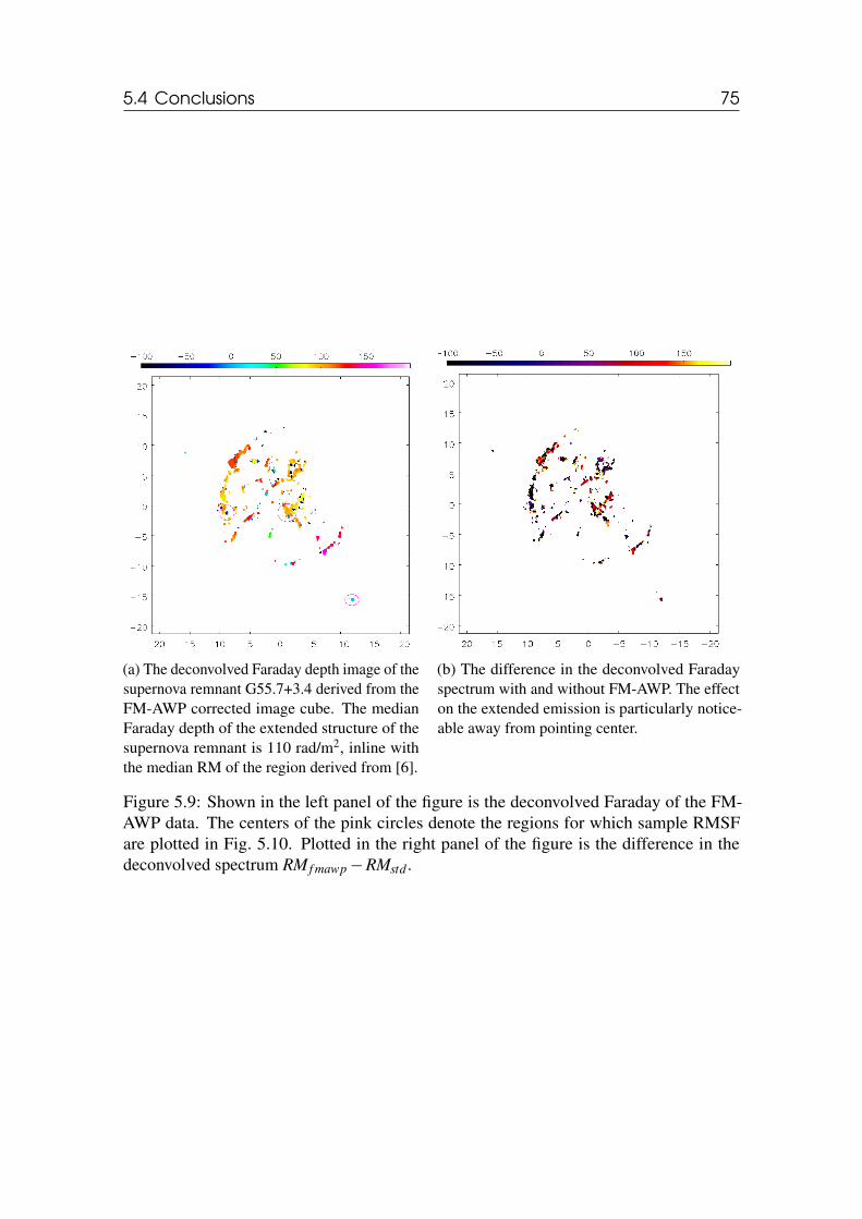
5.4 Conclusions 75
(a) The deconvolved Faraday depth image of thesupernova remnant G55.7+3.4 derived from theFM-AWP corrected image cube. The medianFaraday depth of the extended structure of thesupernova remnant is 110 rad/m2, inline withthe median RM of the region derived from [6].
(b) The difference in the deconvolved Faradayspectrum with and without FM-AWP. The effecton the extended emission is particularly notice-able away from pointing center.
Figure 5.9: Shown in the left panel of the figure is the deconvolved Faraday of the FM-AWP data. The centers of the pink circles denote the regions for which sample RMSFare plotted in Fig. 5.10. Plotted in the right panel of the figure is the difference in thedeconvolved spectrum RM f mawp−RMstd .
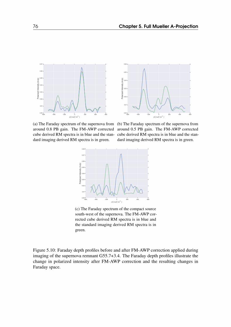
76 Chapter 5. Full Mueller A-Projection
−600 −400 −200 0 200 400 600
φ(rad/m2 )
0.00
0.01
0.02
0.03
0.04
0.05
0.06
0.07
Polarized
Intens
ity (m
Jy)
(a) The Faraday spectrum of the supernova fromaround 0.8 PB gain. The FM-AWP correctedcube derived RM spectra is in blue and the stan-dard imaging derived RM spectra is in green.
−600 −400 −200 0 200 400 600
φ(rad/m2 )
0.00
0.01
0.02
0.03
0.04
0.05
0.06
Polarized
Intens
ity (m
Jy)
(b) The Faraday spectrum of the supernova fromaround 0.5 PB gain. The FM-AWP correctedcube derived RM spectra is in blue and the stan-dard imaging derived RM spectra is in green.
−600 −400 −200 0 200 400 600
φ(rad/m2 )
0.00
0.01
0.02
0.03
0.04
0.05
0.06
0.07
0.08
Polarized
Intens
ity (m
Jy)
(c) The Faraday spectrum of the compact sourcesouth-west of the supernova. The FM-AWP cor-rected cube derived RM spectra is in blue andthe standard imaging derived RM spectra is ingreen.
Figure 5.10: Faraday depth profiles before and after FM-AWP correction applied duringimaging of the supernova remnant G55.7+3.4. The Faraday depth profiles illustrate thechange in polarized intensity after FM-AWP correction and the resulting changes inFaraday space.

5.4 Conclusions 77
algorithm outperforms direction independent imaging methods in both dynamic range andpolarization flux fidelity. Having shown that the FM-AWP method works on simulatedpoint source, I applied it to the VLA supernova remnant G55.7+3.4 data set. The dataclearly show that FM-AWP is better at recovering the true channel polarized intensity (Pi)particularly for point sources farther out in the primary beam. Through Faraday synthesis,I also examined the effect of improper flux reconstruction in polarized intensity for twolines of sights in Faraday depth space. The stark difference for sources located outside theregion of 0.8 PB gain is visible in terms of the shift in the location of the peak in polarizedintensity and the recovered polarized flux density. I show that FM-AWP imaging producesa Faraday depth measurement for the supernova remnant that is consistent with the RMvalue predicted by Taylor et al. [6].

78 Chapter 5. Full Mueller A-Projection
6. Algorithms & Computation
“If you were ploughing a field, which would you rather use ? Two strong oxenor 1024 chicken ?”
—Seymour Cray
Algorithmic development and computational advances proceed in tandem and are truefor the work in this thesis too. The development of a new algorithm requires conceptual-ization, followed by iterative development and testing before a viable algorithm is born.The FM-AWP algorithm started as a conceptual extension of the convolution function pro-duction within the A-Projection framework. All of the code development was carried outwithin the Common Astronomy Software Application (CASA), research and developmentcodebase. One of the primary features of CASA that allowed for this work to be possiblewas the implementation of the parallel mpicasa1. The computational work required forthe completion of the thesis is on two separate fronts, both requiring parallel computation.The first was solving for the ray-traced antenna AIP on a per channel basis for L-Bandholography measurements detailed in Sec. 6.1. The second is an implementation of theFM-AWP algorithm within the CLEAN task framework within CASA.
6.1 Parallel Optimization & Solving for parameterized AIPIn order to solve for antenna AIP, it was necessary to revisit the ray-tracing code thatproduces the per antenna Jones matrix. This is carried out by the BeamCalc module withinCASA. The BeamCalc module contains the ray-tracing code that constructs the antennageometry based on physical parameters that are band specific. From the constructed dishgeometry the ray-tracing produces the AIP for a given frequency and parallactic angle
1https://safe.nrao.edu/wiki/pub/HPC/CasaParallelization/CASA-%204.3-MPI-Parallel-Processing-Framework-Installation-and-advance-user-guide-v1.2.pdf
80 Chapter 6. Algorithms & Computation
specified. The first step was to test the production of the entire Jones matrix given a test dataset. In order to ensure that the code exits after the production of the Jones matrix, (withinthe full imager framework gridding and the first major cycle would immediately follownormally) a test program in C++ was created. The program instantiates the AWProjectFTmodule responsible for WB-AWP and ensures that the BeamCalc module contains therequisite imaging parameters such as the coordinate information of the source, the imagesize, frequency, and resolution. The program wrote to disk both the antenna AIP andimage plane PB matrices. Comparison of the ray-traced theoretical AIP to the measuredPB from holography revealed that the theoretical AIP was underestimating the gain in thefirst side-lobe. In order to solve for the side-lobe as a function of frequency, in terms ofthe input parameters of the antenna geometry in BeamCalc, I modified the calculation ofthe antenna geometry to accept user-defined inputs for pointing offset, central blockageand the taper polynomial for feed illumination. To optimize these parameters I wrote awrapper function in Python that accepted user-defined input values and passed them to thestandalone C++ code. This allowed us to pass the Python wrapper as a function to a scipyminimization routine. The minimization routine traversed the multi-dimensional parameterspace providing parameter values to the ray-tracing code until the parameters converged.This minimization routine for a single frequency channel for one antenna takes 4.5 hoursof runtime to complete running a single thread with sufficient RAM, with minimal disk I/O.Which meant a serial run for 1024 channels in an antenna would take 192 days of runtime.
As the optimization was compute-limited I moved the execution onto a 16 core machineat NRAO compute cluster. Utilizing Python multiprocessing2 libraries an MPI basedPython implementation I parallelized the minimization to run each channel independentlyallowing us to run 16 simultaneous processes on the machine in parallel. Since theparallelization utilizes sub-processes it is a process parallel implementation that reducedthe compute time by a factor if 16. While significant I needed vastly more computationin order to run the optimization for multiple antennas. NRAO data management andsystems (DMS) group provided us access to the Amazon web services (AWS) based on acompute grant they had obtained. Utilizing the AWS compute cluster I was able to run1024 concurrent processes reducing the runtime per-antenna to 6 hours. In this fashion, Icompleted three antennas at a compute cost of nearly $120 per-antenna with a speed up inthe compute time by a factor of 103.
The AWS cluster execution of my code was possible because of the support providedin particular by Erik Bryer and James Robnett of the DMS group. They helped me withcluster management and data transfer between the AWS cluster and NRAO, and in settingup a custom Linux environment required for the installation and execution of the CASAbased code.
6.2 Full Mueller - AW Projection ImplementationThe software implementation of FM-AWP is an extension of the wide-band AW-Projectionsoftware. In this section, I will lay out the framework of the code and the associatedoptimizations that are implemented within CASA that made a working algorithm possible.
The synthesis imaging framework3 within CASA is encapsulated within a high-level
2https://docs.Python.org/2/library/multiprocessing.html3https://casa.nrao.edu/casadocs/casa-5.1.0/global-task-list/task_tclean/about

6.2 Full Mueller - AW Projection Implementation 81
task clean. It accepts user inputs for data, along with the choice of the iterative major andminor cycle algorithms and their termination criteria. The task then performs synthesisimaging on the input data following the imaging equations laid out in chapter 2. CASAhas a base level of C++ code with higher level Python layers made of tools which arein turn used to construct tasks. This layered model allows for swift testing of new ideasin Python before the final implementation is carried out in C++. In order to implementFM-AWP, I restricted ourselves to the existing A-Projection framework. Once a userinvokes A-projection for all Stokes parameters, the clean task triggers the C++ moduleAWProjectFT at the base level. FM-AWP is implemented in the code within this module.In the following pseudocode function in italics highlight, the regions of the code thatrequired changes towards the implementation of the FM-AWP algorithm.
Code Outline Full Mueller A-Projection Module OverviewInitialize the full Stokes model and residual images, determine major cycle algorithm
Major Cycle Algorithm : FM-AWP
1: AWProjectFT2:3: Setup grid and lattice parameters, Stokes parameters4:5: Invoke PolOuterProduct (POP)6: Define hybrid mode Mueller configuration (12 CFs), and initialize POP::init7: POP::MakePolIndex - Map Stokes to feed parameters8: POP::MakeConjPolIndex - Map Stokes to conjugate of feed parameters9: POP::MakePolMat - Initialize the Mueller matrix indices (A)
10: POP::MakeConjPolMat - Initialize Conjugate Mueller indices (AM†)
11: Invoke AWConvFunc(AWCF) module12: AWCF:: findConvFunc - locate cached CF.
13: AWCF:: makeConvFunc. - calls VLACalcIlluminationConvFunc (VCICF)14: VCICF: applyPB - Determine frequency, PA, CF size - Invoke BeamCalc.15: BeamCalc::skyMueller - Ray traced Jones matrix per-antenna, PA, spw.16: VCICF::makeMueller - Mueller matrix for the baseline i− j, per PA, per spw.17: Pass CF and data to the gridder - AWVisResampler(AWVR) module18: AWVR::accumulateToGrid the forward step to produce gridded visibilities19: Pass visiblity buffer(subset) and CF to fortranized gridding loops20: AWVR::accumulateFromGrid the reverse step to produce de-gridded visibilities21: Pass gridded visiblity buffer(subset) and CF to fortranized de-gridding loops
The progression of the code development was both linear and modular. Initial changeswere performed within the AWConvFunc (AWCF) module (refer pseudocode shown) toimplement the ray-traced AIP, which formed the focus of the chapters 3 and 4. Uponsuccessful testing of the CF’s produced by the code, I implemented the PolOuterProduct
82 Chapter 6. Algorithms & Computation
(POP) module to ensure the polarization mapping between the correlations in the visibilityand the imaging Stokes parameters for hybrid mode. The hybrid mode excludes the secondorder anti-diagonal term of the Mueller matrix, thus reducing the total number of termsper row of the Mueller matrix from 4 to 3. As a final step, I altered the AWVisResampler(AWVR) gridding and de-gridding module to accept the visibility to Stokes mapping andensured that it was passed on to the Fortranized loops which perform the gridding basedonly on the mappings specified.
The CF production in full Mueller A-Projection as implemented in CASA is on a perspectral window basis (typically 16 to 32 spectral windows across a VLA observing band).While higher spectral resolution CF production is possible, the necessary changes in codehave not been implemented at the task level of CASA till date. The CFs are producedonce at the start of the imaging and are cached by AWProjectFT. Parallelization of theCF production is what made the FM-AWP testing a reality. The parallelization of theCF production utilizes the parallel MPI CASA imaging module developed by the CASAhigh-performance computing group along with the CASA algorithms group. Along withthe MPI parallelization, additional changes were carried out to enable smarter cachedCF management which allows for only the CF used in the gridding of the subset of datato be read in rather than reading in the entirety of the cache and holding the cache inmemory. While these are extremely important updates it must be noted that FM-AWPalgorithm development only played a role in testing the implementation of the memorymanagement code. The smart CF cache was developed by the CASA algorithms R&Dgroup independent of the efforts to develop the FM-AWP algorithm.
In a typical A-Projection imaging cycle, 80% of the time is spent in the gridding of thedata. The convolution function production is a significantly lesser fraction of the imagingruntime and is a one time cost. With the parallelization, of the gridder through MPIframework in CASA, the gridding cost can now be distributed across multiple processorsand nodes efficiently. The parallelization offers a scalable solution for addressing theincreased computational complexity of the projection algorithms. With the rise in theavailability of computing infrastructure (AWS, Google Cloud), parallel implementationsof interferometric imaging algorithms are the way forward.

7. Conclusion
“We can only see a short distance ahead, but we can see plenty there that needsto be done.”
—Alan Turing
In line with the thesis goals outlined in chapter 1, I have developed a Projectionalgorithm (FM-AWP) that corrects for the effects of the Mueller matrix during the courseof the imaging major cycle. I demonstrated the effects of the instrumental Mueller matrixon polarimetric imaging with particular emphasis on Faraday synthesis in chapter 3. Ideveloped a frequency-dependent high spectral resolution model of the antenna AIP to beused within the FM-AWP as a part of the convolution function production in chapter 4. Idemonstrated the workings of the FM-AWP on VLA data in chapter 5. In the followingsections 7.1, I will summarize the work required to achieve FM-AWP algorithm and itscurrent capabilities and limitations and examine the road ahead for further algorithmicdevelopment in Sec. 7.2
7.1 Full Mueller A-Projection & Polarimetric ImagingThe initial stage of the FM-AWP algorithm was to evaluate the effect of the Mueller matrixon imaging. I characterized the error induced in polarized flux due to the time-varyingMueller matrix through simulation of point sources distributed across the field of viewof the antenna PB for the VLA. The tests showed that flux leakage from Stokes -I into-Q and -U is significant up to 10% of the total intensity. Furthermore, I show that theleakage changes with the changing PA for an alt-az mounted telescope such as the VLA.Long integration observations of ∆PA > 100 leads to a reduction in the polarization fluxleakage due to averaging. However, flux leakage vanishes only for a perfectly symmetricalhour angle coverages around the meridian or for observations with ∆PA = 180. I also
84 Chapter 7. Conclusion
demonstrated that for realistic beam models with measurable second-order effects, suchas beam squash, averaging of polarization leakage does not go to zero for ∆PA = 180.I also examined the role of off-axis polarization leakage in the antenna PB in Faradayspace and showed that it manifests as a peaked signal near RM of 0 rad m−2. For realisticextragalactic sources with a Faraday space signatures ranging ±100 rad m−2, the off-axispolarization leakage acts as a distorting signal in the Faraday space. The distorted signalcauses confusion for deconvolution algorithms such as RM Clean. FM-AWP algorithmcorrects for these off-axis effects provided a model of the antenna AIP as a function oftime, frequency and polarization are available.
In the second stage of the FM-AWP algorithm development, I considered ray-tracedantenna AIP models that can be supplied as convolution functions to the algorithm tocorrect for the effects of the full Mueller matrix. The models did not reflect the frequency-dependent structure (such as a standing wave) across the bandwidth of L, S and C bandsseen in Holographic measurements. In order to bridge the difference between the measuredPB and the PB derived from the model AIP, I carried out parameter optimization of physi-cally motivated antenna parameters. The parameters being optimized were the antennapointing off-set, tapering of the feed illumination and the radius of the central apertureblockage. The parameters capture the frequency-dependent variations of the antenna PBper channel out to the first-side lobe. The optimized parameters were fit as a function offrequency using a straight line and sine function for the central blockage parameter. The fitcaptured the presence of a standing wave 17 MHz in frequency arising from a secondaryreflection between the feed and the antenna secondary. The aperture illumination parame-ters were fit also with straight lines. This resulted in a highly compressed representation ofthe frequency-dependent behavior of the AIP (and consequently the PB). I also performedpoint source simulations to demonstrate that the frequency dependence of the antenna PBis required for high fidelity high dynamic range imaging for dynamic ranges of 100000:1or higher.
As a culmination of the algorithmic work, I introduced the FM-AWP algorithm. Itutilizes the unitary nature of the Jones matrix to project out the effects of the full Muellermatrix. I demonstrated the existence of the normalizable projection operator AM†(ν∗)?A(ν) = Tr(A)21, for the narrowband and broadband instances of the algorithm. FM-AWP in the narrowband case reduces the off-diagonal elements (F †Ai j, i 6= j) of theMueller matrix down to 4× 10⁻⁵ in the narrowband implementation and 8.4× 10⁻⁵ inthe broadband implementation. Through point source simulations of radio deep fields,I showed that for crowded fields with many clustered sources the FM-AWP algorithmoutperforms standard imaging (Cotton-Schwab CLEAN). Sources of known polarizedflux were simulated to create a measurement set that was imaged using FM-AWP andstandard imaging. The ratio of the recovered flux to the input flux was plotted as histogramsin the case of Stokes -Q, -U and in polarized intensity. Imaging with FM-AWP led totightly distributed histograms around unity while standard imaging resulted in extremelywidely distributed denoting poor flux fidelity in terms of imaging. I then applied theFM-AWP algorithm to VLA data of the supernova remnant G55.7+3.4. FM-AWP reducedthe depolarization due to the time-variable primary beam and removed flux leaking fromStoke -I into Stokes -Q and -U as demonstrated by the polarized intensity images.
In order to perform Faraday synthesis, the supernova remnant was imaged per spectralwindow to produce an image cube with both FM-AWP and standard imaging. The resulting
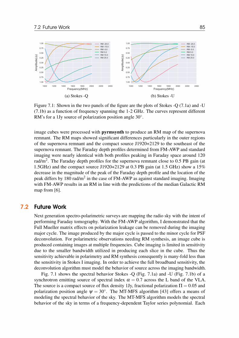
7.2 Future Work 85
1000 1200 1400 1600 1800 2000 2200 2400Frequency(MHz)
−1.00
−0.75
−0.50
−0.25
0.00
0.25
0.50
0.75
1.00
Amplitu
de(Jy)
RM -25.0RM -15.0RM -5.0RM 5.0RM 15.0RM 25.0
(a) Stokes -Q
1000 1200 1400 1600 1800 2000 2200 2400Frequency(MHz)
−1.00
−0.75
−0.50
−0.25
0.00
0.25
0.50
0.75
1.00
Amplitu
de(Jy)
RM -25.0RM -15.0RM -5.0RM 5.0RM 15.0RM 25.0
(b) Stokes -U
Figure 7.1: Shown in the two panels of the figure are the plots of Stokes -Q (7.1a) and -U(7.1b) as a function of frequency spanning the 1-2 GHz. The curves represent differentRM’s for a 1Jy source of polarization position angle 30.
image cubes were processed with pyrmsynth to produce an RM map of the supernovaremnant. The RM maps showed significant differences particularly in the outer regionsof the supernova remnant and the compact source J1920+2129 to the southeast of thesupernova remnant. The Faraday depth profiles determined from FM-AWP and standardimaging were nearly identical with both profiles peaking in Faraday space around 120rad/m2. The Faraday depth profiles for the supernova remnant close to 0.5 PB gain (at1.5GHz) and the compact source J1920+2129 at 0.3 PB gain (at 1.5 GHz) show a 15%decrease in the magnitude of the peak of the Faraday depth profile and the location of thepeak differs by 180 rad/m2 in the case of FM-AWP as against standard imaging. Imagingwith FM-AWP results in an RM in line with the predictions of the median Galactic RMmap from [6].
7.2 Future WorkNext generation spectro-polarimetric surveys are mapping the radio sky with the intent ofperforming Faraday tomography. With the FM-AWP algorithm, I demonstrated that theFull Mueller matrix effects on polarization leakage can be removed during the imagingmajor cycle. The image produced by the major cycle is passed to the minor cycle for PSFdeconvolution. For polarimetric observations needing RM synthesis, an image cube isproduced containing images at multiple frequencies. Cube imaging is limited in sensitivitydue to the smaller bandwidth utilized in producing each slice in the cube. Thus thesensitivity achievable in polarimetry and RM synthesis consequently is many-fold less thanthe sensitivity in Stokes I imaging. In order to achieve the full broadband sensitivity, thedeconvolution algorithm must model the behavior of source across the imaging bandwidth.
Fig. 7.1 shows the spectral behavior Stokes -Q (Fig. 7.1a) and -U (Fig. 7.1b) of asynchrotron emitting source of spectral index α = 0.7 across the L band of the VLA.The source is a compact source of flux density 1Jy, fractional polarization Π = 0.05 andpolarization position angle ψ = 30. The MT-MFS algorithm [43] offers a means ofmodeling the spectral behavior of the sky. The MT-MFS algorithm models the spectralbehavior of the sky in terms of a frequency-dependent Taylor series polynomial. Each
86 Chapter 7. Conclusion
term of the frequency-dependent polynomial (nterms ≥ 2) are gridded and deconvolvedseparately (for details refer Rau and Cornwell [43]) and the resultant images are used toreconstruct the spectral behavior of the source in total intensity such as the spectral indexor spectral curvature. The MT-MFS framework extended to polarization would allow forthe modeling of the frequency dependence of Stokes -Q and -U in terms of the Taylorpolynomial. The fitted polynomials terms beyond the first (intensity in that polarization)can be modeled for different kinds of intervening plasma models (such as Faraday "thin"or Faraday "thick") and compared to the imaged data. This imaging method will allowfor a) greater sensitivity (full bandwidth used in imaging), b) resolution (no smoothingrequired during spectral modeling). c) reduced overall computation (deconvolution isnot per channel like in cube imaging but rather per term) and, d) faster Faraday spaceidentification of the source model.
It can be seen that polynomial fits are not the ideal basis for fitting Stokes -Q and -Uin the presence of larger rotation measures (RM ≥ |±25|) from Fig. 7.1. Alternatively,Fourier basis functions(sine and cosine) fitted to the source in wavelength squared spacewould allow us to model the source spectral behavior in Stokes -Q and -U for all measurablerotation measures. This would also result in an improved linear polarized intensity imagealong with fits to the Faraday space behavior of each source in the field of view. Such amethod will allow for easy classification of sources in wide-field broadband surveys of thesky planned with the next generation of radio telescopes since most of the source in thesky ( 75% of the detected sources) are Faraday "thin" sources [25]. A polarized MTMFSalgorithm is then a means of performing Stokes -Q and -U fitting in a model-independentfashion.
I have demonstrated the FM-AWP imaging method for the VLA, in general, it isapplicable to other parabolic dish arrays such as the GMRT, MeerKAT, ASKAP, SKA andthe ngVLA. The FM-AWP algorithm in its current form needs rigorous implementationand testing before integration within CASA for use by the wider user community. Imagingwith the FM-AWP algorithm for other telescope arrays can be incorporated through theinclusion of their respective antenna AIP. With the antenna AIP incorporated in the FM-AWP code framework, high fidelity wide-field broadband polarimetric imaging for thenext-generation of spectro-polarimetic surveys would be possible.
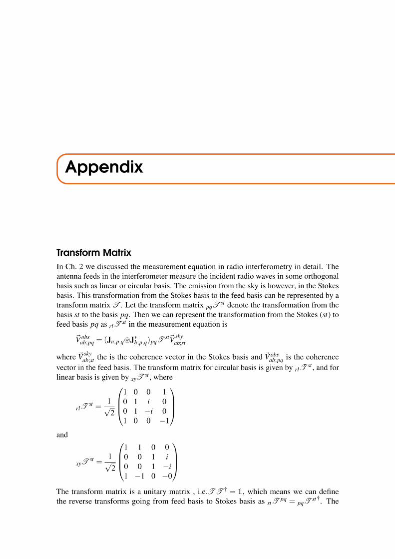
Appendix
Transform MatrixIn Ch. 2 we discussed the measurement equation in radio interferometry in detail. Theantenna feeds in the interferometer measure the incident radio waves in some orthogonalbasis such as linear or circular basis. The emission from the sky is however, in the Stokesbasis. This transformation from the Stokes basis to the feed basis can be represented by atransform matrix T . Let the transform matrix pqT st denote the transformation from thebasis st to the basis pq. Then we can represent the transformation from the Stokes (st) tofeed basis pq as rlT
st in the measurement equation is
~V obsab;pq = (Ja;p,q~J∗b;p,q)pqT
st~V skyab;st
where ~V skyab;st the is the coherence vector in the Stokes basis and ~V obs
ab;pq is the coherencevector in the feed basis. The transform matrix for circular basis is given by rlT
st , and forlinear basis is given by xyT st , where
rlTst =
1√2
1 0 0 10 1 i 00 1 −i 01 0 0 −1
and
xyTst =
1√2
1 1 0 00 0 1 i0 0 1 −i1 −1 0 −0
The transform matrix is a unitary matrix , i.e.T T † = 1, which means we can definethe reverse transforms going from feed basis to Stokes basis as stT pq = pqT st†. The
88 Chapter 7. Conclusion
transform matrix for circular basis is given by stT rl , and for linear basis is given by stT xy,where
stTrl =
1√2
1 0 0 10 1 i 00 −i i 01 0 0 −1
and
stTxy =
1√2
1 0 0 11 0 0 −10 1 1 00 −i i −0
The transform matrix provides the instantaneous transformation from one basis to another.In the case of an Alt-Az mounted antenna, there is an additional parallactic angle rotationthat needs to be included in the transform matrix. If the antenna parallactic angle is χ , thetransform matrix due to the parallactic angle rotation for a baseline can be given in termsof the individual antenna parallactic angles as,
Tχ =
(eiχa 00 e−iχa
)⊗(
eiχb 00 e−iχb
)∗=
ei(χa+χb) 0 0 0
0 ei(χa−χb) 0 00 0 ei(χb−χa) 00 0 0 e−i(χa+χb)
The effective transform matrix in the case of an Alt-Az mounted antenna is then Tχ · pqT st .

Bibliography
Books4F. F. Chen, Introduction to Plasma Physics and Controlled Fusion (1984) (cit. on p. 8).
27A. G. Pacholczyk, Radio astrophysics. Nonthermal processes in galactic and extragalac-tic sources (1970) (cit. on p. 12).
30G. B. Taylor, C. L. Carilli, and R. A. Perley, eds., Synthesis Imaging in Radio AstronomyII, Vol. 180, Astronomical Society of the Pacific Conference Series (1999) (cit. on pp. 19,53).
31A. R. Thompson, J. M. Moran, and G. W. Swenson, Jr., Interferometry and Synthesis inRadio Astronomy, 3rd Edition (2017) (cit. on p. 21).
38R. N. Bracewell, The Fourier transform and its applications (2000) (cit. on p. 28).
Articles1C. L. Carilli, and G. B. Taylor, “Cluster Magnetic Fields”, Annual Reviews of Astronomy& Astrophysics 40, 319–348 (2002) (cit. on p. 7).
2D. M. Palmer, S. Barthelmy, N. Gehrels, R. M. Kippen, T. Cayton, C. Kouveliotou, D.Eichler, R. A. M. J. Wijers, P. M. Woods, J. Granot, Y. E. Lyubarsky, E. Ramirez-Ruiz,L. Barbier, M. Chester, J. Cummings, E. E. Fenimore, M. H. Finger, B. M. Gaensler, D.Hullinger, H. Krimm, C. B. Markwardt, J. A. Nousek, A. Parsons, S. Patel, T. Sakamoto,G. Sato, M. Suzuki, and J. Tueller, “A giant γ-ray flare from the magnetar SGR 1806 -20”, Nature 434, 1107–1109 (2005) (cit. on p. 7).
3B. J. Burn, “On the depolarization of discrete radio sources by Faraday dispersion”,Monthly Notices of the Royal Astronomical Society 133, 67 (1966) (cit. on pp. 8, 41).
90 Chapter 7. Conclusion
5M. A. Brentjens, and A. G. de Bruyn, “Faraday rotation measure synthesis”, Astronomy& Astrophysics 441, 1217–1228 (2005) (cit. on pp. 8, 9, 41).
6A. R. Taylor, J. M. Stil, and C. Sunstrum, “A Rotation Measure Image of the Sky”, TheAstrophysical Journal 702, 1230–1236 (2009) (cit. on pp. 8, 10, 42, 74, 75, 77, 85).
7J. J. Condon, W. D. Cotton, E. W. Greisen, Q. F. Yin, R. A. Perley, G. B. Taylor, and J. J.Broderick, “The NRAO VLA Sky Survey”, The Astronomical Journal 115, 1693–1716(1998) (cit. on pp. 8, 37).
8N. Oppermann, H. Junklewitz, G. Robbers, M. R. Bell, T. A. Enßlin, A. Bonafede,R. Braun, J. C. Brown, T. E. Clarke, I. J. Feain, B. M. Gaensler, A. Hammond, L.Harvey-Smith, G. Heald, M. Johnston-Hollitt, U. Klein, P. P. Kronberg, S. A. Mao,N. M. McClure-Griffiths, S. P. O’Sullivan, L. Pratley, T. Robishaw, S. Roy, D. H. F. M.Schnitzeler, C. Sotomayor-Beltran, J. Stevens, J. M. Stil, C. Sunstrum, A. Tanna, A. R.Taylor, and C. L. Van Eck, “An improved map of the Galactic Faraday sky”, Astronomy& Astrophysics 542, A93, A93 (2012) (cit. on pp. 8, 10).
9N. Oppermann, H. Junklewitz, M. Greiner, T. A. Enßlin, T. Akahori, E. Carretti, B. M.Gaensler, A. Goobar, L. Harvey-Smith, M. Johnston-Hollitt, L. Pratley, D. H. F. M.Schnitzeler, J. M. Stil, and V. Vacca, “Estimating extragalactic Faraday rotation”, As-tronomy & Astrophysics 575, A118, A118 (2015) (cit. on p. 8).
10J. E. Kooi, P. D. Fischer, J. J. Buffo, and S. R. Spangler, “VLA Measurements of FaradayRotation through Coronal Mass Ejections”, Solar Physics 292, 56, 56 (2017) (cit. onp. 9).
11A. H. Savage, S. R. Spangler, and P. D. Fischer, “Probing the Rosette Nebula StellarBubble with Faraday Rotation”, The Astrophysical Journal 765, 42, 42 (2013) (cit. onp. 9).
12C. R. Purcell, B. M. Gaensler, X. H. Sun, E. Carretti, G. Bernardi, M. Haverkorn,M. J. Kesteven, S. Poppi, D. H. F. M. Schnitzeler, and L. Staveley-Smith, “A Radio-Polarisation and Rotation Measure Study of the Gum Nebula and Its Environment”, TheAstrophysical Journal 804, 22, 22 (2015) (cit. on p. 9).
13A. H. Costa, S. R. Spangler, J. R. Sink, S. Brown, and S. A. Mao, “Denser Samplingof the Rosette Nebula with Faraday Rotation Measurements: Improved Estimates ofMagnetic Fields in H II Regions”, The Astrophysical Journal 821, 92, 92 (2016) (cit. onp. 9).
14S. A. Mao, N. M. McClure-Griffiths, B. M. Gaensler, J. C. Brown, C. L. van Eck, M.Haverkorn, P. P. Kronberg, J. M. Stil, A. Shukurov, and A. R. Taylor, “Magnetic Fieldsin the Milky Way Halo”, Highlights of Astronomy 16, 403–403 (2015) (cit. on p. 9).
16J. M. Lawler, and B. Dennison, “On intracluster Faraday rotation. II - Statistical analysis”,The Astrophysical Journal 252, 81–91 (1982) (cit. on p. 9).
17D. D. Sokoloff, A. A. Bykov, A. Shukurov, E. M. Berkhuijsen, R. Beck, and A. D.Poezd, “Depolarization and Faraday effects in galaxies”, Monthly Notices of the RoyalAstronomical Society 299, 189–206 (1998) (cit. on p. 9).
18G. Heald, R. Braun, and R. Edmonds, “The Westerbork SINGS survey. II Polarization,Faraday rotation, and magnetic fields”, Astronomy & Astrophysics 503, 409–435 (2009)(cit. on p. 9).
7.2 Future Work 91
19J. M. Stil, M. Krause, R. Beck, and A. R. Taylor, “The Integrated Polarization of SpiralGalaxy Disks”, The Astrophysical Journal 693, 1392–1403 (2009) (cit. on p. 9).
20D. Farnsworth, L. Rudnick, and S. Brown, “Integrated Polarization of Sources at λ ˜ 1m and New Rotation Measure Ambiguities”, The Astronomical Journal 141, 191, 191(2011) (cit. on p. 9).
21D. Mesa, C. Baccigalupi, G. De Zotti, L. Gregorini, K.-H. Mack, M. Vigotti, and U.Klein, “Polarization properties of extragalactic radio sources and their contribution tomicrowave polarization fluctuations”, Astronomy & Astrophysics 396, 463–471 (2002)(cit. on p. 9).
22A. R. Taylor, J. M. Stil, J. K. Grant, T. L. Landecker, R. Kothes, R. I. Reid, A. D. Gray,D. Scott, P. G. Martin, A. I. Boothroyd, G. Joncas, F. J. Lockman, J. English, A. Sajina,and J. R. Bond, “Radio Polarimetry of the ELAIS N1 Field: Polarized Compact Sources”,The Astrophysical Journal 666, 201–211 (2007) (cit. on p. 9).
23C. A. Hales, R. P. Norris, B. M. Gaensler, and E. Middelberg, “ATLAS 1.4 GHz datarelease 2 - II. Properties of the faint polarized sky”, Monthly Notices of the RoyalAstronomical Society 440, 3113–3139 (2014) (cit. on p. 9).
24L. Rudnick, and F. N. Owen, “The Distribution of Polarized Radio Sources greater than15 microJy in GOODS-N”, The Astrophysical Journal 785, 45, 45 (2014) (cit. on p. 9).
25C. J. Law, B. M. Gaensler, G. C. Bower, D. C. Backer, A. Bauermeister, S. Croft, R.Forster, C. Gutierrez-Kraybill, L. Harvey-Smith, C. Heiles, C. Hull, G. Keating, D.MacMahon, D. Whysong, P. K. G. Williams, and M. Wright, “Spectropolarimetry withthe Allen Telescope Array: Faraday Rotation Toward Bright Polarized Radio Galaxies”,The Astrophysical Journal 728, 57, 57 (2011) (cit. on pp. 9, 86).
26S. P. O’Sullivan, S. Brown, T. Robishaw, D. H. F. M. Schnitzeler, N. M. McClure-Griffiths, I. J. Feain, A. R. Taylor, B. M. Gaensler, T. L. Landecker, L. Harvey-Smith,and E. Carretti, “Complex Faraday depth structure of active galactic nuclei as revealedby broad-band radio polarimetry”, Monthly Notices of the Royal Astronomical Society421, 3300–3315 (2012) (cit. on pp. 9, 43).
28J. P. Hamaker, J. D. Bregman, and R. J. Sault, “Understanding radio polarimetry. I.Mathematical foundations.”, Astronomy & Astrophysics, Supplements 117, 137–147(1996) (cit. on pp. 19, 34).
29U. Rau, S. Bhatnagar, M. A. Voronkov, and T. J. Cornwell, “Advances in Calibrationand Imaging Techniques in Radio Interferometry”, IEEE Proceedings 97, 1472–1481(2009) (cit. on pp. 19, 24, 27).
32S. Bhatnagar, Cornwell, K. Golap, and J. M. Uson, “Correcting direction-dependentgains in the deconvolution of radio interferometric images”, Astronomy & Astrophysics487, 419–429 (2008) (cit. on pp. 23, 27, 30, 47–49).
33S. Bhatnagar, U. Rau, and K. Golap, “Wide-field wide-band Interferometric Imaging:The WB A-Projection and Hybrid Algorithms”, The Astrophysical Journal 770, 91, 91(2013) (cit. on pp. 23, 27, 30, 47, 57, 69).
34T. J. Cornwell, and P. N. Wilkinson, “A new method for making maps with unstable radiointerferometers”, Monthly Notices of the Royal Astronomical Society 196, 1067–1086(1981) (cit. on p. 24).
92 Chapter 7. Conclusion
35T. Cornwell, “Recommendation for the AIPS++ Imaging Model”, AIPS++ Note Series148 (1992) (cit. on p. 24).
36T. Cornwell, “The Generic Interferometer I : Overview of Calibration and Imaging”,AIPS++ Note Series 183 (1995) (cit. on p. 24).
37T. Cornwell, “The Generic Interferometer II: Image Solvers”, AIPS++ Note Series 184(1995) (cit. on p. 24).
40T. J. Cornwell, K. Golap, and S. Bhatnagar, “The Noncoplanar Baselines Effect in RadioInterferometry: The W-Projection Algorithm”, IEEE Journal of Selected Topics in SignalProcessing 2, 647–657 (2008) (cit. on p. 30).
41B. Humphreys, and T. Cornwell, “Analysis of Convolutional Resampling AlgorithmPerformance”, SKA Memo Series 132 (2011) (cit. on p. 30).
43U. Rau, and T. J. Cornwell, “A multi-scale multi-frequency deconvolution algorithm forsynthesis imaging in radio interferometry”, Astronomy & Astrophysics 532, A71, A71(2011) (cit. on pp. 30, 85, 86).
44P. Jagannathan, S. Bhatnagar, U. Rau, and R. Taylor, “Direction-Dependent Effects InWide-Field Wideband Full-Stokes Radio Imaging”, Astronomical Society of the PacificConference Series 495, edited by A. R. Taylor, and E. Rosolowsky, 379 (2015) (cit. onpp. 33, 34).
45U. Rau, S. Bhatnagar, and F. N. Owen, “Deep Wideband Single Pointings and Mosaicsin Radio Interferometry: How Accurately Do We Reconstruct Intensities and SpectralIndices of Faint Sources?”, The Astronomical Journal 152, 124, 124 (2016) (cit. onpp. 33, 67, 70).
46D. McConnell, J. R. Allison, K. Bannister, M. E. Bell, H. E. Bignall, A. P. Chippendale,P. G. Edwards, L. Harvey-Smith, S. Hegarty, I. Heywood, A. W. Hotan, B. T. Indermuehle,E. Lenc, J. Marvil, A. Popping, W. Raja, J. E. Reynolds, R. J. Sault, P. Serra, M. A.Voronkov, M. Whiting, S. W. Amy, P. Axtens, L. Ball, T. J. Bateman, D. C.-J. Bock,R. Bolton, D. Brodrick, M. Brothers, A. J. Brown, J. D. Bunton, W. Cheng, T. Cornwell,D. DeBoer, I. Feain, R. Gough, N. Gupta, J. C. Guzman, G. A. Hampson, S. Hay, D. B.Hayman, S. Hoyle, B. Humphreys, C. Jacka, C. A. Jackson, S. Jackson, K. Jeganathan,J. Joseph, B. S. Koribalski, M. Leach, E. S. Lensson, A. MacLeod, S. Mackay, M.Marquarding, N. M. McClure-Griffiths, P. Mirtschin, D. Mitchell, S. Neuhold, A. Ng, R.Norris, S. Pearce, R. Y. Qiao, A. E. T. Schinckel, M. Shields, T. W. Shimwell, M. Storey,E. Troup, B. Turner, J. Tuthill, A. Tzioumis, R. M. Wark, T. Westmeier, C. Wilson,and T. Wilson, “The Australian Square Kilometre Array Pathfinder: Performance ofthe Boolardy Engineering Test Array”, Publications of the Astron. Soc. of Australia 33,e042, e042 (2016) (cit. on p. 37).
47A. R. Taylor, S. J. Gibson, M. Peracaula, P. G. Martin, T. L. Landecker, C. M. Brunt,P. E. Dewdney, S. M. Dougherty, A. D. Gray, L. A. Higgs, C. R. Kerton, L. B. G. Knee,R. Kothes, C. R. Purton, B. Uyaniker, B. J. Wallace, A. G. Willis, and D. Durand, “TheCanadian Galactic Plane Survey”, The Astronomical Journal 125, 3145–3164 (2003)(cit. on p. 37).

7.2 Future Work 93
48J. C. Brown, A. R. Taylor, R. Wielebinski, and P. Mueller, “On Large-Scale MagneticField Reversals in the Outer Galaxy”, The Astrophysical Journal Letters 592, L29–L32(2003) (cit. on p. 42).
49R. Perley, “Jansky Very Large Array Primary Beam Characteristics”, VLA Memo 196(2016) (cit. on pp. 43, 51).
50C. Heiles, P. Perillat, M. Nolan, D. Lorimer, R. Bhat, T. Ghosh, E. Howell, M. Lewis,K. O’Neil, C. Salter, and S. Stanimirovic, “All-Stokes Parameterization of the MainBeam and First Sidelobe for the Arecibo Radio Telescope”, Publications of the Astron.Soc. of Pacific 113, 1247–1273 (2001) (cit. on pp. 43, 52, 57).
51A. Popping, and R. Braun, “The standing wave phenomenon in radio telescopes. Fre-quency modulation of the WSRT primary beam”, Astronomy & Astrophysics 479, 903–913 (2008) (cit. on p. 47).
52P. Jagannathan, S. Bhatnagar, U. Rau, and A. R. Taylor, “Direction Dependent Correc-tions in Polarimetric Radio Imaging I : Characterizing the effects of the primary beamon full Stokes imaging”, ArXiv e-prints (2017) (cit. on pp. 47, 57).
53W. Brisken, “Using Grasp8 to study the VLA beam”, VLA Memo 58 (2003) (cit. onpp. 48, 50).
54R. A. Perley, and B. J. Butler, “An Accurate Flux Density Scale from 50 MHz to 50GHz”, The Astrophysical Journal Supplements 230, 7, 7 (2017) (cit. on pp. 51, 72).
55R. A. Perley, and B. J. Butler, “Integrated Polarization Properties of 3C48, 3C138, 3C147,and 3C286”, The Astrophysical Journal Supplements 206, 16, 16 (2013) (cit. on pp. 51,72).
56J. A. Nelder, and R. Mead, “A Simplex Method for Function Minimization”, TheComputer Journal 7, 308–313 (1965) (cit. on p. 51).
57E. Momjian, R. Perley, and R. Hayward, “The Impact of the New Thermal Gap ReceiverAssembly on the Sensitivity of the EVLA at L-Band (1?2 GHz)”, VLA Memo 165 (2014)(cit. on p. 52).
58 Astropy Collaboration, T. P. Robitaille, E. J. Tollerud, P. Greenfield, M. Droettboom,E. Bray, T. Aldcroft, M. Davis, A. Ginsburg, A. M. Price-Whelan, W. E. Kerzendorf,A. Conley, N. Crighton, K. Barbary, D. Muna, H. Ferguson, F. Grollier, M. M. Parikh,P. H. Nair, H. M. Unther, C. Deil, J. Woillez, S. Conseil, R. Kramer, J. E. H. Turner,L. Singer, R. Fox, B. A. Weaver, V. Zabalza, Z. I. Edwards, K. Azalee Bostroem, D. J.Burke, A. R. Casey, S. M. Crawford, N. Dencheva, J. Ely, T. Jenness, K. Labrie, P. L.Lim, F. Pierfederici, A. Pontzen, A. Ptak, B. Refsdal, M. Servillat, and O. Streicher,“Astropy: A community Python package for astronomy”, Astronomy & Astrophysics558, A33, A33 (2013) (cit. on p. 54).
59S. Bhatnagar, U. Rau, D. A. Green, and M. P. Rupen, “Expanded Very Large ArrayObservations of Galactic Supernova Remnants: Wide-field Continuum and Spectral-index Imaging”, The Astrophysical Journal Letters 739, L20, L20 (2011) (cit. on pp. 57,72).
60S. Bhatnagar, and T. Cornwell, “Solving for Antenna Based Pointing Errors”, EVLAMemo Series 84 (2004) (cit. on p. 60).

94 Chapter 7. Conclusion
61S. Bhatnagar, and T. J. Cornwell, “The Pointing Self Ccalibration Algorithm for ApertureSynthesis Radio Telescopes”, The Astronomical Journal (2017) (cit. on p. 60).
62M. R. Bell, and T. A. Enßlin, “Faraday synthesis. The synergy of aperture and rotationmeasure synthesis”, Astronomy & Astrophysics 540, A80, A80 (2012) (cit. on p. 73).

List of Figures
1.1 The sky in rotation measure . . . . . . . . . . . . . . . . . . . . . . . . . . . . . . . . . . . . . 101.2 The polarization ellipse is shown in the xy plane. Where a and b are thesemi-major and semi-minor axes of the ellipse. ψ is the inclination of thesemi-major axis of the ellipse with respect to the local x coordinate axis. 131.3 The Poincaré sphere of a polarization vector P(2ψ,2β ) is shown. TheCartesian axes, S1, S2 and S3, form the Stokes parameter axes, as theprojection of the P along each of the axes gives rise to the polarized Stokesparameters. . . . . . . . . . . . . . . . . . . . . . . . . . . . . . . . . . . . . . . . . . . . . . . . . . . . . . . . . 14
3.1 Amplitude of the image domain complex Mueller Matrix for an arbi-trary baseline a−b at the VLA at 1.5GHz. The color scale is a logarithmicscale spanning nine orders of magnitude. The Mueller elements are com-puted using the normalized Jones matrix for the diagonal elements to havea peak value of unity along the pointing direction. The direction of thearrows have been reversed from [44] to be more in line with the vectornotation in [28]. . . . . . . . . . . . . . . . . . . . . . . . . . . . . . . . . . . . . . . . . . . . . . . . . . . . . 343.2 The direction dependent Mueller in Stokes basis at 1.5 GHz. The im-ages show sign(Mab)× (log10(abs(Mab)) and the color scales is shown as theexponent of 10. The leading order terms are along the diagonal. The I<-Vand V<-I term (due to polarization squint) are ∼ 2 orders of magnitudelower than the diagonal. The I<-Q and I<-U terms (due to off-axis beampolarization) are ∼ 2.5− 3 orders of magnitude lower than the diagonalterms. . . . . . . . . . . . . . . . . . . . . . . . . . . . . . . . . . . . . . . . . . . . . . . . . . . . . . . . . . . . . . . 353.3 The imaging simulations followed the methodology outlined in the flowdiagram. The sky model image was multiplied by the Fourier transform ofthe Mueller matrix for a change in parallactic angle of 5 . . . . . . . . . . . . . 37

96 LIST OF FIGURES
3.4 The visibility amplitude of RR (convex curves) and LL (concave curves)of an unpolarized source situated at the half-power point at the referencefrequency 1.5 GHz. The RR and LL show different amplitudes due to thesquint of the VLA antennas. The color axis represents 6 spectral windows,spanning from 1 GHz (blue) to 2 GHz (red) in steps of 0.2 GHz . . . . . . . . 38
3.5 Polarized flux density in RL and LR as a function of parallactic angle forthe unpolarized source at the half-power point at 1.5 GHz. Colors are as inFig 3.4. The signal arise from angle-dependent leakage from the sourcetotal intensity signal and also has strong frequency dependence as thesource moves out through the PB with increasing frequency. RL and LR areboth complex-valued with the same amplitude. These curves thereforeoverlap exactly . . . . . . . . . . . . . . . . . . . . . . . . . . . . . . . . . . . . . . . . . . . . . . . . . . . . 39
3.6 Polarized flux in RL and LR as a function of parallactic angle for the 5%polarized source at the same location of the unpolarized source in Fig.3.5.Colors are as in Fig. 3.4. RL and LR are both complex-valued with the sameamplitude. These curves therefore overlap exactly . . . . . . . . . . . . . . . . . . . 39
3.7 The amplitude of fractional polarization (QM/IM) as a function of theinterval of parallactic angle during observations. The solid lines representthe unpolarized point source at the half power point(at 1.5 GHz). Thedotted lines represent the polarized point source of input Stokes Q/I of0.0353. Colors are as in Fig. 3.4 . . . . . . . . . . . . . . . . . . . . . . . . . . . . . . . . . . . . . . 40
3.8 As in Fig. 3.7 but for UM/IM. . . . . . . . . . . . . . . . . . . . . . . . . . . . . . . . . . . . . . 40
3.9 As in Fig. 3.7 but for ΠL . . . . . . . . . . . . . . . . . . . . . . . . . . . . . . . . . . . . . . . . . 41
3.10 The FDF of the instrumental leakage for the unpolarized source atthe PB half power point at 1.5 GHz. In this plot the color now denotesincreasing parallactic angle intervals spanned from 36 (blue) to 180 (red).The instrumental signal is maximum close to a Faraday depth of zero. Thesignal amplitude decreases for observations with increasing ∆χ. . . . . . . 42
3.11 Plotted is the linear polarized intensity of the polarized source (ΠL=0.05,ψ = 22.5, RM=0 rad m−2) at PB the power point at 1.5 GHz, as a function ofrotation measure. The color axis denotes the different parallactic angleintervals spanned from 0 to 180 degrees. The spread in the RM around zeroarises from the addition of the beam RM to the intrinsic source polarization.43
3.12 Plotted is the linear polarized intensity of a polarized source (P=0.05,ψ = 22.5, RM=100) at half power at 1.5 GHz, as a function of rotation mea-sure. The color axis denotes the different parallactic angle intervals spannedfrom 0 to 180 degrees. . . . . . . . . . . . . . . . . . . . . . . . . . . . . . . . . . . . . . . . . . . . . . . 43
3.13 Plotted is the leakage flux at the half power of the PB at 1.5GHz, asa fraction of Stokes I for different parallactic angle intervals ∆χ. The dot-ted(squashed) and solid(ideal) in red represent leakage into to polarizedintensity ΠL, the blue lines represent the Stokes U and the green lines theStokes Q. . . . . . . . . . . . . . . . . . . . . . . . . . . . . . . . . . . . . . . . . . . . . . . . . . . . . . . . . . . . 44

LIST OF FIGURES 97
4.1 A VLA Antenna is shown with the feeds and the obstructing structs,along with the two parameters used to model the AIP accurately a) theapparent central blockage (Rhole), b) the feed illumination taper. Theexact physical model parameters used to derive the dish geometry aredescribed in Table. 4.1 . . . . . . . . . . . . . . . . . . . . . . . . . . . . . . . . . . . . . . . . . . . . . . 494.2 The upper panel images shows the residuals (normalized with respectto peak intensity at the beam center) of |EHolo
~I−F †Aideal
~I| measured at
1.353 GHz. The upper left panel show the residual for the left-circular (L)polarization and the upper right panel for the right-circular (R). Similarly, thelower panels shows |EHolo
~I−F †AM
~I|. . . . . . . . . . . . . . . . . . . . . . . . . . . . . . . . . . . 53
4.3 Fit to the recovered apparent blockage parameter for antennas 6,10, 12, in red, green and blue respectively, with the lines representing thefit and the points represent the derived apparent blockage data across448 MHz, of data. . . . . . . . . . . . . . . . . . . . . . . . . . . . . . . . . . . . . . . . . . . . . . . . . . . . 544.4 The dashed red, green and blue lines show the feed taper function at1, 1.5 and 2.0 GHz respectively, used to derive Aideal
~I. The solid, red, green
and blue (overwritten by the dashed red line) lines show the feed taperfunction at 1, 1.5 and 2.0 GHz respectively, used to derive AM
~Ifor antenna
12. . . . . . . . . . . . . . . . . . . . . . . . . . . . . . . . . . . . . . . . . . . . . . . . . . . . . . . . . . . . . . . . . . 554.5 Plotted are the pointing offsets for antennas 6, 10, 12, in blue, greenand red respectively, for R and L polarizations of the antennas aroundzero. The offsets are in percentage of the HPBW of the antenna. The linesrepresent the actual pointing vectors of the antennas and is obtained byfitting the per channel pointing solutions with a best fit line. The regionswith no solutions between 1.4 and 1.65 GHz corresponds to two spectralwindows with noisy solutions due to the presence of strong radio frequencyinterference. . . . . . . . . . . . . . . . . . . . . . . . . . . . . . . . . . . . . . . . . . . . . . . . . . . . . . . 56
4.6 Plotted is the fractional change in the antenna PB,(PBde f −PBTrue)/PBTrue,
with magenta contours overlaid of PBTrue at 80, 50, 10, 5 and 1 % powerat 1.448 GHz of antenna 12. The left panel is the fractional change intotal intensity, while the panel on the right is the fractional change in linearpolarized intensity . . . . . . . . . . . . . . . . . . . . . . . . . . . . . . . . . . . . . . . . . . . . . . . . . . 56
4.7 Plotted is the fractional change in the antenna wideband PB,(PBTrue−PBde f )/PBTrue
across 1 GHz of bandwidth, with magenta contours overlaid of PBTrue at 80,50, 10, and 1 % power at the reference frequency,1.5 GHz of antenna 12.584.8 The panels of the figure shows the off diagonal antenna Jones matrixelement R← L of EM
i = F †[AMi ], with the upper panels show the real portion
of EMi and the lower panels show the imaginary part of EM
i at 1.013 GHzof antenna 27. The left most panels (upper and lower) EM
i that includesan optimized second-order polynomial in phase. The figures in the centerof the complex EM
i , includes an ≈ 18 rotation in addition to the second-order polynomial in phase. In the two panels on the right the the real andimaginary parts of the measured holographic EM
i is shown. . . . . . . . . . . . 59

98 LIST OF FIGURES
4.9 Plotted in the figure is the PB corrected point source flux. Plotted inblue are the full Mueller imaged and PBTrue corrected point source fluxes forthe parameterized frequency-dependent model. Plotted in green is the fullMueller imaged and PBde f corrected point source fluxes for the frequencyindependent model. . . . . . . . . . . . . . . . . . . . . . . . . . . . . . . . . . . . . . . . . . . . . . . . 60
4.10 The difference image ITrue− Ide f . The white circles mark the locationsof the points sources in the image. The color scales from −1×10⁻⁴Jy/beamto 1×10⁻⁴Jy/beam. . . . . . . . . . . . . . . . . . . . . . . . . . . . . . . . . . . . . . . . . . . . . . . . . . . 61
5.1 Complex baseline AIP displayed in matrix form. . . . . . . . . . . . . . . . . . 65
5.2 The inverted matrices post FM-AWP. . . . . . . . . . . . . . . . . . . . . . . . . . . . . . 66
5.3 Plotted in the figure is a profile through the FM-AWP corrected imageof the first off-axis leakage element F †A32
M ?A01. The the blue curve is anazimuthal slice through the narrowband leakage residuals post FM-AWPand the green curve is an azimuthal slice through the wide-band correctionF †A32
M (ν∗)?A01(ν), post FM-AWP. . . . . . . . . . . . . . . . . . . . . . . . . . . . . . . . . . . . . . 67
5.4 The panels shows a comparison of deep field imaging in Stokes I,without FM-AWP (left panel) and with FM-AWP (right Panel). The dashedcontours represent the 80% (inner circle) and 50% in the PB. . . . . . . . . . . 68
5.5 The panels shows a comparison of deep field imaging in Stokes Vwithout FM-AWP (left panel) and with FM-AWP (right Panel). The noise inFM-AWP corrected image is a factor of 10 lower and the color scaling forthe panel has been saturated to show the noise in the image. The scalebar has units of mJy for the left panel and units of ×10−1 mJy for the rightpanel. The dashed contours represent the 80% (inner circle) and 50% in thePB. . . . . . . . . . . . . . . . . . . . . . . . . . . . . . . . . . . . . . . . . . . . . . . . . . . . . . . . . . . . . . . . . . 69
5.6 The panels provide a comparison of deep field imaging in polarizedintensity (P =
√Q2 +U2) without full Mueller A-Projection(left panel) and with
full Mueller A-projection(right Panel) . . . . . . . . . . . . . . . . . . . . . . . . . . . . . . . . . 70
5.7 Histogram of the ratio of the reconstructed flux values, in Stokes I andin linear polarized intensity P are plotted in the panels on the left. The errorin the reconstructed flux density in Stokes I and polarized flux density isplotted against the model flux density in the panels on the right. In eachof the cases FMAWP imaged sources are plotted in blue and the standardimaged sources in green. . . . . . . . . . . . . . . . . . . . . . . . . . . . . . . . . . . . . . . . . . . . 71
5.8 The panels provide a comparison of the wide-band polarized intensityimage of the supernova remnant through standard imaging (left panel)and with FM-AWP(right Panel). The mask in the FM-AWP image is at a PBgain of 0.01 . . . . . . . . . . . . . . . . . . . . . . . . . . . . . . . . . . . . . . . . . . . . . . . . . . . . . . . . 73
5.9 Shown in the left panel of the figure is the deconvolved Faraday of theFM-AWP data. The centers of the pink circles denote the regions for whichsample RMSF are plotted in Fig. 5.10. Plotted in the right panel of the figureis the difference in the deconvolved spectrum RM f mawp−RMstd. . . . . . . . 75

LIST OF FIGURES 99
5.10 Faraday depth profiles before and after FM-AWP correction appliedduring imaging of the supernova remnant G55.7+3.4. The Faraday depthprofiles illustrate the change in polarized intensity after FM-AWP correctionand the resulting changes in Faraday space. . . . . . . . . . . . . . . . . . . . . . . . . 76
7.1 Shown in the two panels of the figure are the plots of Stokes -Q (7.1a)and -U (7.1b) as a function of frequency spanning the 1-2 GHz. The curvesrepresent different RM’s for a 1Jy source of polarization position angle 30.85

100 LIST OF FIGURES


