Discrete-Time Geo/G/2 Queue under a Serial and Parallel Queue Disciplines

Discrete-Time Geo/G/2 Queue under a Serialand Parallel Queue Disciplines

Sivasamy Ramasamy, Onkabetse A. Daman and Sulaiman Sani ∗

Abstract—This article discusses the steady stateanalysis of a heterogeneous server queuing systemcalled the Geo/G/2 queue. We supposed that arrivalsoccur according to a geometric process to receive ser-vice on server-1 according to a geometric service timedistribution with mean rate μ or on server-2 accord-ing to a general distribution B(t) with mean rate μ2.There are two queue disciplines employed for servicenamely; the serial queue discipline (queue discipline-I) and the parallel queue discipline (queue discipline-II). Using the embedded method when the disciplineis serial and the supplementary variable techniquewhen it is parallel, we present an exact analysis of thearrival distribution. Furthermore, the actual waitingtime expectations are derived and approximated. Ouranalysis can be applied in managing service systemsin many areas of communication, telecommunications,business and computer systems where services are dis-crete in nature for instance, in the performance evalu-ation and design of buffers for statistical multiplexers,traffic concentrators, switch modules, networks.

Keywords: Geometric arrival, Geo/G/2 queue,Geo/(Geo+G)/2 queue, Geo/Geo,G/2 queue.

1 Introduction

We study a geometric arriving and general service timequeuing system1 called the Geo/G/2 queue with twoservers modeled as server-1 and server-2. This kind ofqueuing system is a model of slots with finite bound-aries where at most only one arrival (customer) oc-curs in a given time (late arrival) for service. We sup-pose that arrivals (customers, packets, inputs) and ser-vice times (length of service) are integer multiples of agiven slot. This implies that departures only occur atthe other end of the slot. The service and inter-arrivaldurations between consecutive arrivals are measured asrandom numbers of slot durations. This give rise to a

∗Sivasamy Ramasamy is a Professor of Statistics currently withthe Department of Statistics, University of Botswana-Gaborone.His field of research is Stochastic modeling & Analysis. OnkabetseA. Daman is a senior Lecturer and the former HOD, Dept. of Math-ematics, University of Botswana-Gaborone. His area of research isStochastic Processes, Mathematical Analysis & Applications. Su-laiman Sani is a Research Scholar in the Department of Mathe-matics, University of Botswana-Gaborone. His area of researchis on Stochastic modeling with bias in Queuing theory. Email:[email protected]: Manuscript submitted February 2015.

1Under two distinct queue disciplines.

discrete-time queuing system of the form Geo/Geo+G/2or Geo/Geo,G/2 depending on the schedule for service(queue discipline). Now, suppose that the proposed queu-ing systems have an infinite number of waiting positionswith server-1 faster than server-2. Then, an interestingfeature of this investigation is that, it derives the discreteresults of this work to the corresponding continuous timeversion M/G/2 queues analyzed in Sivasamy, Daman &Sulaiman [15].

Normally, discrete-time scaling (small time scale) andtheir corresponding models often reflect an underlying ap-plication. For example, the clock time unit in a computersystem, the fixed size data units (bits, bytes, fixed lengthpackets) on a communication channel. Similarly, for suf-ficiently small slot lengths, discrete-time queuing modelsare approximations for the corresponding models wherethe time scale is continuous. Furthermore, asynchronoustransfer mode (ATM) multiplexers and broadband in-tegrated service digital network (B-ISDN) are used totransfer data sets, voice and video communications ondiscrete-time basis. In both the multiplexers and theB-ISDN for instance, the time axis is normally dividedinto slots (fixed-length of continuous intervals called slotsof unit length (right-end boundary=left end boundary)).Takagi [17] indicated that this type of models is essen-tially the best choice for analyzing computer and commu-nication systems. Bruneel & Kim [5] compared some fea-tures of discrete-time parallel queuing models with thatof the continuous ones and indicated that in continuous-time parallel queuing models, the probability that an ar-rival and a departure occurring simultaneously in a verysmall time interval is zero. This is not so in discrete-timemodels where both events can occur simultaneously at aboundary epoch of a slot. Under this added advantage,it requires that the order of occurrence be taken care of;that is either arrival first (AF) or departure first (DF).Hence, the need to study such models for the benefit ofcomputers or telecommunication systems such as the onesexemplified above.

The literature on discrete-time queuing models is enor-mous. Over the years, a lot of research has been carriedout. For a survey of related ones, see Takagi [17], Bruneel[4], Bruneel & Kim [5], Ishizaki, Takine & Hasegawa [10],Bruneel, Walraevens, Claeys, & Wittevrongel [6], Briem,Theimer, & Kroner [3]. Precisely, Briem, Theimer & Kro-

IAENG International Journal of Applied Mathematics, 45:4, IJAM_45_4_14

(Advance online publication: 14 November 2015)

______________________________________________________________________________________

ner [3] studied a discrete-time single server queuing sys-tem with a non-renewal customer process and providedan exact analysis of both the infinite and the finite ca-pacity queue yields in terms of the state probabilities atdeparture instants as well as the loss probability. Theresults show that one can obtain interesting results forqueues under discrete-time scaling assumption. For moreon single server discrete queuing systems, see Bruneel [5],Ishizaki, Takine & Hasegawa [10]. Similarly, works onmulti-server queuing systems with discrete-time scalinghave grown tremendously in the last two decades. For asurvey of related ones; see Goswami & Mund [8], Artalejo& Lopez Herrero [1], Goswami [7].

Now, what can be observed in these and many other liter-ature sources on multi-server models under discrete timeassumption is the adoption of the FCFS queue discipline.This assumption may not be realistic. For instance, ifa telecommunication system or device provides servicewith varying speeds, then arriving packets might be pre-ferred to be allocated the fastest device for service. Onthe other hand, if allocated the slowest device randomly,then there is a possibility that packets entering the sys-tem after the one allocated to the slow device to clearout earlier by obtaining service from the device with afaster working rate. Apparently in this case, the FCFSqueue discipline is violated due to heterogeneity in ser-vice speeds of the two working devices. This and similarreal life scenarios make the adoption of the FCFS queuediscipline unrealistic in multi-server discrete-time queu-ing systems with embedded heterogeneity because of thehigh probability of violation therein. Hence, there is theneed for designing alternative queue disciplines that canreduce the impact of the violation so that the resultingwaiting times of customers in this kind of queuing sys-tems are almost identical with that of the FCFS.

Our motivation to study these kind of models stemmedfrom the several applications of the models working un-der the proposed queue disciplines giving rise to either theGeo/Geo+G/2 or Geo/Geo,G/2 queuing models respec-tively. Specific examples of application scenarios includecomputer systems, communication systems, telecommu-nication networks, production management, BroadbandIntegrated Services Digital Network (BISDN), dynamicbandwidth allocation and flexible capacity allocation. Inthese systems, information is digitized and segmentedinto small packets arranged serially or in parallel. There-fore, analyzing models for such systems is an excellenttool for decision making relative to congestion man-agement for better service delivery. Interestingly, un-like in many models designed with similar assumptions,here, the effects of the two queue disciplines can all becomputed2. Most importantly, the analysis of the dis-crete time Geo/Geo,G/2 queue carried out is relativelyclose to that of Boxma, Deng & Zwart [2] and Krish-

2Both analytically and numerically.

namoorthi [11] but more convenient for application incommunications and modern computer systems. In thissense, each queue discipline here is an excellent alter-native for use in our real life applications. Precisely,the model under queue discipline-I is called the dis-crete time Geo/Geo + G/2 with serialized servers andthe model under queue discipline-II is called the discretetime Geo/Geo,G/2 queue with parallel servers. Withthis structuring, our work stands to benefit both the ser-vice provider and the customer through efficient resourcemanagement in the former and minimization of waitingtimes in the later.

1.1 Basic Assumptions

We suppose that a slot of unit length is given suchthat arrivals occur on slot boundaries according to anArrival First (AF) policy. Marking the time axis by0, 1, 2, .., t, ..., and supposing that these arrivals occur at0−, 1−, , t−, time points such that a service starts onlyat slot boundaries with each service duration taking anumber of slots. In addition, an arrival can leave thesystem upon service completion only3. Furthermore, weassumed that potential departures occur at slot bound-aries at 0+, 1+, ..., t+, .... instants. Denote the time be-tween successive arrivals (the inter-arrival time) by A.For a detail description of the discrete time concepts em-ployed here, see Gupta & Goswami [9] who modeled asingle-server bulk service queue with finite buffer spacein a discrete-time environment and provided the analysisunder both arrival first (AF) and departure first (DF)management policies and distributions of buffer contentat various epochs. Such management policies play a sig-nificant role in the determination of steady-state proba-bilities relating to the number of arrivals in the system(queue) at special epochs (e.g., arrival, departure, and ar-bitrary epochs) and hence, they affect performance mea-sures to a great extent. Now, assuming that the num-ber of arrivals in successive slots are independent andidentically distributed (i.i.d.) random variables (derivedfrom a Geometric (or Bernoulli) Arrival Process:) sub-ject to the condition that only one arrival occurs in aslot with probability λ; (0 < λ < 1). This assump-tion ensures that the inter-arrival time A is geometricallydistributed4 with mean 1

λ and probability distributionP (A = k slots) = λ(1−λ)k−1 for k = 1, 2, ... Denote fur-ther by A(z), the probability generating function (PGF)of inter-arrival times and by L(z), the PGF of the numberof arrivals in a slot such that

A(z) =λz

1− (1− λ)z; |z| < 1, L(z) = 1− (1− z)λ (1)

Now, if it is supposed that for arrivals serviced by server-1, the service time S1 follows the geometric distribution

3No reneging, balking by arrivals in the system.4We further suppose that S1 and S2 are mutually independent

with each other and the inter-arrival time distribution.



______________________________________________________________________________________

with probability mass function f1(k) = P (S1 = k) =μ(1−μ)k−1; k = 1, 2, ... with mean 1

μ per slot. Then the

PGF of S1 and the corresponding Ls(z) representing thePGF of the number of departures in a slot are respectivelygiven by5

F1(z) =

∞∑k=1

μ(1− μ)k−1zkμz

1− (1− μ)z(2)

Let the service times S2 of arrivals serviced by server-2follows a general distribution f2(k) = P (S2 = k) withPGF

F2(z) =

∞∑k=1

f2(z)zk; |z| < 1 (3)

If the mean service time is β with rate μ2 = 1β , then

one can provide an analysis for this discrete queuing sys-tem similar to that carried out in Sivasamy, Daman &Sulaiman [15] in the continuous-time case.

1.2 The Serial Queue Discipline

This is a new proposal of connecting the servers in series6

subject to the following:

1 If an arrival enters into an idle system, his serviceis immediately initiated by server-1. This arrival isserved by server-1 at a constant rate μ if no otherarrival occurs during his on-going service period.

2 Otherwise if at least one more arrival occurs be-fore his service completed, then the first arrival isserved jointly by both servers according to the ser-vice time distribution fmin(k) = P (Smin ≤ k),where Smin = Min(S1, S2) and the PGF of Smin

denoted by Fmin(z) given by7

Fmin(z) =

∞∑k=1

fmin(k)zk (4)

The expected values of S1, S2 and Smin are respectivelygiven by E[S1] = F ′

1(z) = 1μ , E[S2] = F ′

2(1) = β = 1μ2

and E[Smin] = F ′min(1). For example, if the service time

S2 of arrivals on server-2 is a geometric random variablewith mean 1

μ2, then the mean of Smin derived from (4) is

equal to8

5In this case, |z| < 1, Ls(z) = 1− (1− z)μ.6Queue Discipline-17Further simplification of (4) yields Fmin(z) = F1(z) + F2((1−

μ)z)(1− F1(z))8Similarly, the service rate of Smin = μ+μ2−μμ2,since there is

a positive probability of serving an arrival simultaneously by bothservers just before the end of a slot boundary.

E[Smin] = F ′min(1) =

1

μ+ μ2 − μμ2

Lemma 1.1 If no arrival is served simultaneously andthe service time for all arrivals is equivalent to some kslots, then the service (or departure) rate r(k) offered bythe combined service time distributions f1(k) and f2(k)of the serialized servers in the Geo/Geo + G/2 queuingsystem is given by

r(k) =f1(k)

1− P (S1 < k)+

f2(k)

1− P (S2 < k)(5)

Proof Suppose ρ = λμ < 1. Then a closed form expres-

sion for r(k) can be obtained for particular cases of f2(k)like the Geometric, Negative-binomial, or Phase (PH)type distributions. Suppose that the service time dis-tribution of arrivals served by the slow server (server-2)is any of the distributions mentioned above with a finitemean. Then our discussion follows viz;

1.3 Negative-binomial Distribution

Suppose that the service time S2 is a Negative-Binomial NB(α, β) random variable with mass functionb(k;α, μ2) = P (S2 = k). Let S2 denotes the number ofslots required to complete a service by server-2 at the αth

success in a sequence of independent Bernoulli trials withprobability of success v ∈ (0 < v < 1), then

b(k;α, v) =(k−1α−1

)vα(1− v)k−α; k = α, α+ 1, ...

The mean of S2 is denoted by E[S2] =αv and the variance

by V ar[S2] =α(1−v)

v2 . Similarly, the mean service rate μ2

is given by vα . Finally, the service (or departure) rate

r(k) offered by the combined service time distributionsf1(k) and f2(k) of serialized servers of the Geo/Geo +NB(α, v)/2 queuing system is given by9 μ+ v

α .

Corollary 1.2 Suppose that 1μ2

→ ∞. Then the

Geo/Geo+G/2→Geo/Geo/1.

Queuing models operating under conditions (1) through(4) above are a discrete-time class of the Geo/Geo+G/2queues.

1.4 The‘Parallel Queue‘Discipline

Here, we adopt the queue discipline in Krishnamoorthi[11] that minimizes the violation of the FCFS principle for

9One can carryout similar analysis for the above mentioned dis-tributions also.



______________________________________________________________________________________

a two heterogeneous server queue subject to the conditionthat the mean service rates of server-1 and server-2 are μand μ2 respectively. If an arrival occurs and find:

1. Both servers free; it occupies server-I (assuming thatserver-1 gives faster service on average).

2. Server-1 is engaged; it waits for service from server-Iwhether or not server-II is free. But if the number ofarrivals waiting for service from server-I becomes m(a positive integer), it goes to server-2 if that serveris free; otherwise it waits as the (m+ 1)th arrival inthe queue. Note that the first m arrivals in the queuewill be getting service from server-1 and the (m+1)th

arrival in the queue will go to server-2 if that serverbecomes free prior to the finishing of service of thearrival in server-1. Otherwise he will move up as themth arrival in the queue. Hence may decide to takeservice from server-1.

3. Both servers are engaged and a queue of length ngreater than or equal to m is formed; It joins thequeue as the (n+ 1)th arrival. All arrivals after themth arrival in the queue take a decision only whenthey reach the (m+ 1)th position in the queue. Thedecision is taken according to the rule mentioned in2 of server-I engaged above.

The positive integer m is to be chosen such that it isone less than the greatest integer in the ratio μ

μ2. It

is clear for this choice of m that: When there are marrivals10 waiting for service from server-I, an incomingarrival finds it profitable to go to server-2 if that serveris free since (m+2)μ−1 < μ−1

2 . Similarly, when there areonly (m−1) arrivals waiting for service from server-1, anincoming arrival will find it profitable to join the queuefor service from server-1, even if server-2 is free, since(m+1)μ−1 < μ−1

2 . In case μ

μ−12

is an integer, then μ

μ−12

−1,

so that joining the queue for service from server-1 is notany more or any less profitable than going to server-2 ifthe server is free. But there is no harm in assuming thateven in this case, the arrival joins the queue for servicefrom server-1 when there are only (m−1) arrivals waitingfor service.

Thus, this queue discipline achieves the objective thatthe least amount of waiting time is spent in the systemaccording to the conditions present upon its arrivals andalso reduces the violation of first-in first-out principle.In section 3, we consider the discrete-time Geo/Geo,G/2queue under the above queue discipline with m = 1 andsubject to the following time constraints that:

1. The service time is divided into slots numbered as0, 1, 2, ..., ..., η with each slot of unit length.

10We analyze the case for m = 1 customer.

2. A potential arrival occurs in an interval (η−, η) whilea potential departure served by either server-1 or byserver-2 occurs in the interval (η, η+) as consideredin Gupta & Goswami [9].

3. The state of the queue length process is defined atdeparture epoch η+ by two random variables N(η+)denoting the number of arrivals in the system at timeη+ and η is past service time of the arrival servedby server-2 if any.

The rest of the work is organized as follows; in sectiontwo, we derive the PGFs of the number of arrivals presentin the system, the waiting time distribution and theirmean values. Section 3 highlights the various specialfeatures of the proposed methodology on the analysis oftwo paralleled heterogeneous servers Geo/Geo,G/2 sys-tem which does not violate the FCFS principle. Section4 gives a concluding report and in section five, we givea conjecture that takes the results of this work to an-other model of interesting application similar to the onesdiscussed in this work.

2 The Geo/G/2 Queue under 1.2

Here, we consider ’the embedded time points’ generatedat departure instants of arrivals just after a service com-pletion either by server-1 or by server-2. Hence thesequence of system states observed at these embeddedpoints with state representation Nk = N(tk) denotingthe number of arrivals left behind in the queue by the kth

departing arrival at departure epoch tk forms a MarkovChain {Nk} with state space S = 0 , 1 , ....

2.1 PGF for the Number of Arrivals

Let qj be the steady state probability of finding j arrivalsin the system as observed by a departing arrival with az-transform V (z) =

∑j=∞j=0 qjz

j . Similarly, let αj denotesthe probability that j arrivals occur in a service comple-tion period with probability mass function fmin(k) andδj denotes the probability that j arrivals occur in a geo-metrically distributed service time with probability massfunction f1(k). Since these arrivals come from a geomet-ric process at a steady rate λ, then for j = 1, 2, 3, ..., wehave

αj =

∞∑k=1

fmin(k)(kj

)λj(1− λ)k−j (6)

and

δj =

∞∑k=1

f1(k)(kj

)λj(1− λ)k−j (7)



______________________________________________________________________________________

Now, denote the respective z-transforms of the probabil-ity distributions {αj} and {δj} by Amin(z) and A1(z)respectively such that

Amin(z) =

∞∑j=0

αjzj = Fmin(1− λ+ λz) (8)

and

A1(z) =

∞∑j=0

δjzj = F1(1− λ+ λz) (9)

Focusing on the embedded points under equilibrium con-ditions, let the unit step conditional transition proba-bility of the system going from state i of the (k − 1)st

embedded point to state j in the kth embedded point beqij = P (Nk = j/Nk−1 = i); i, j ∈ S . These transitionprobabilities will form a unit step transition probabilitymatrix Q = qij as below:

Q =

⎛⎜⎜⎜⎜⎝

δ0 δ1 δ2 δ3 . . . .δ0 δ1 δ2 δ3 . . . .0 α0 α1 α2 α3 . . .0 0 α0 α1 α2 α3 . .0 0 0 α0 α1 α2 α3 .

⎞⎟⎟⎟⎟⎠ (10)

If we denote by qj = limn→∞ qnij , the equilibrium stateprobabilities at departure instants where qnij representsthe n-step probability of moving from state i to j suchthat Q = qij with q = (q0, q1, q2, ...) and e = (1, 1, 1, ...)

′,.

Assuming that A′min(1) < 1, then the stationary dis-

tribution of the state transition matrix Q exits and isgiven by the unique solution of the following system ofequations:

qQ = q,qe = 1 (11)

Now, multiplying the jth equation of qQ = q in (11)by zj and summing all the left-hand sides and the right-hand sides from j = 0 to j = ∞, we get the PGF Vmin(z)of the queue length distribution qj of the sequence {Nk}below11

Vmin(z) =q1z[Amin(z)−A1(z)] + q0[Amin(z)−D]

Amin(z)− z(12)

Since q1 = ρq0, A′min(1) < 1, A′

1(1) = ρ and V (1) = 1,we derive from (12) that

Vmin(z) =(z − 1)A1(z) + (1 + ρz)[A1(z)−Amin(z)]

z −Amin(z)(13)

And12 the mean number E[N ] of arrivals present in thesystem at a random point or at a departure epoch of time

11D = zA1(z)

12Here, q0 =1−A

′min(1)

1+(ρ−A′min

(1))(1+ρ)

is13

E[N ] =

(ρ−A

′min(1)

) [ρ+A

′min(1)(1 + ρ)

]1 + (ρ−A

′min(1))(1 + ρ)

+K (14)

The14 discrete time equivalent of PASTA (Poison Ar-rivals See Time Averages) is referred to as BASTA(Bernoulli Arrivals See Time Averages) or GASTA (Geo-metric Arrivals See Time Averages). Using this property,we envisage that the distribution Vmin(z) in (13) also holdfor the number of arrivals in the system as seen by an ar-bitrary arrival entering the system. Now, if we denotethe PGF of the waiting time W representing the num-ber of slots for which an arrival stays in the system withdistribution W (k) = P (W = k) by W (z) for 0 < z < 1.Then replacing 1− (λ−λz) by z in (13), one obtains that

Vmin(z) = W (1− λ+ λz) (15)

And the mean waiting time of an arrival in the systemobtained from (15) satisfies the well-known Little’s for-mula. For a numerical illustration, suppose that λ variesfrom 5 to 15 as in Table-1 below while μ=8.0, μ2=7.5,the following numerical values are obtained:

Table-1: Mean queue Length E(N) and Meanwaiting Time W̄

μ = 8.0 and μ2 = 7.5

λ ρ ρ1 q0 E[N ] W̄5 0.63 0.32 0.45 1.01 0.208 1.00 0.52 0.25 2.05 0.2610 1.25 0.65 0.15 3.12 0.3111 1.38 0.71 0.11 3.90 0.3512 1.50 0.77 0.08 5.04 0.4213 1.63 0.84 0.05 6.97 0.5414 1.75 0.90 0.03 11.2 0.8015 1.88 0.97 0.01 32.0 2.14

From table-1, it can be seen that both the mean queuelength E[N] and the mean waiting time W̄ steadily in-crease with increase in λ. Also, the stationary q0 valuesdecrease with increase in λ as expected.

Lemma 2.1 Suppose server-2 breaks down during an op-erational period. Then the Geo/Geo+G/2 → Geo/Geo/1queue.

Proof Suppose that the load ρ = λμ < 1. Denote by

Q0(z) and W0(z) the PGFs of the queue length and thewaiting time distributions of the Geo/Geo/1 system suchthat

Q0(z) =(1− z)(1− ρ)F1(1− λ = λz)

F1(1− λ = λz)− z(16)

13This measure is obtained after differentiating the above equa-tion at z=1.

14K=ρ+[A

′min(1)]2

1−A′min

(1)



______________________________________________________________________________________

with mean

E[N ] = ρ+λ2

2(1− ρE(S1(S1 − 1)) (17)

Similarly, let

W0(z) =(1− z)(1− ρ)F1(z)

(1− z)− λ(1− F1(z))(18)

with mean

W̄0 =E[N ]

λ(19)

Now, if server-2 breaks down, then the service situationis equivalent to a long service time of mean service timeβ = ∞ units. Consequently, F2(z) cannot exist. Puttingμ2=0 in (4) and an onward simplification, one obtainsthat Amin(z) = F1(1 − λ + λz) = A1(z). Finally, thelemma follows if Amin(z) is replaced by A1(z) in the PGFof the queue length distribution Vmin(z) in (13).

3 The Geo/G/2 Queue under 1.4

We will now discuss the steady state analysis of theGeo/Geo,G/2 queue under the parallel queue disciplineoutlined above for m = 1 arrival. The analysis is carriedout using the past service time of the arrival being servedby server-2 as a supplementary variable.

Denote by N the steady state number of arrivals in thesystem and by ζ the steady state past service time ofthe current arrival on server-2. Looking at the system atdeparture instants, then the bi-variate process {N, ζ} is aMarkov process with state space S = 0 , 1 , 2 , ...× [0 ,∞).Suppose that P is a probability measure such that

R0 = P [Both servers are idle]

R1,0 = [Only Server − 1 is busy; N = 1]

R0,1(η) = P [Only Server − 2 is busy; N = 1]

R1,1(η) = P [Both Servers are busy; N = 2]

R1,1,0 = P [Only Server − 1 is busy; N = 2]

and that15

R1,1,1(η) = P [Both Servers are busy, N = 3]

Remark We assign η to Rj only when server-2 is busy.Given that two or more customers are present in the sys-tem and that their past service time lies in (η, η + dη)then in steady state, Rj(η) → Rj .

We give the steady state difference equations (56)through (66) in terms of the above probability measuresthat describe the queue length process in Appendix A.

15For any Rj when both servers are busy, the supplementaryvariable ζ is such that η ≤ ζ < η + dη.

3.1 Difference Operator

Let Δ denotes the forward type finite difference operatorthat is; Δf(x) = f(x+1)−f(x) for a real valued functionf(x). Analogous to rules for finding the derivative, wehave: If c is a constant, then Δc = 0. Similarly, for twoconstants a and b define Δ(af + bg) = aΔf + bΔg andΔ(fg) = fΔg + gΔf +ΔgΔf.16

3.1.1 The Stationary PGF P(z)

Let, for j = (0, 1), (1, 1), (1, 1, 1), 4, 5, ,

Qj(η) =Rj(η)

1−B(η)(20)

and that

R̃j =

∞∑η=0

Qj(η)ΔB(η); Q̃j = βR̃j (21)

Similarly, let

Q∗j (z) =

∞∑η=0

Qj(η)zη (22)

Substituting the quantities defined by (20), (21) and (22)into the equations provided by (56) through (66) of Ap-pendix A coupled with the application of the product rulefor two functions specified above, one obtains the follow-ing set of steady state equations:

λR0 = μR1,0 +1

βQ̃0,1 (23)

(λ+ μ)R1,0 = λR0 + μR1,1,0 +1

βQ̃1,1 (24)

(λ+ μ)R1,1,0 = λR1,0 +1

βQ̃1,1,1 (25)

ΔQ0,1(η) = −λQ0,1(η) + μQ1,1(η) (26)

Q0,1(0+) = 0 (27)

ΔQ1,1(η) = −(λ+ μ)Q1,1(η) + λQ0,1(η) + L (28)

Q1,1(0+) = 0 (29)

ΔQ1,1,1(η) = −(λ+ μ)Q1,1,1(η) + λQ1,1(η) +M (30)

16The ΔfΔg term is ignored in queuing applications.



______________________________________________________________________________________

Q1,1,1(0+) = λR1,1,0 +1

βQ̃4 (31)

And17 for j=4,5,..., we have18

ΔQj(η) = −(λ+ μ)Qj(η) + λQj−1(η) + H (32)

Qj(0+) =1

βQ̃j+1 (33)

To solve (23) through (33), multiply each Qj(η) by anappropriate zη : |z| < 1 and summing as in (22). Oneobtains following difference equations19

(1

z− 1

)Q∗

0,1(z) + λQ∗0,1(z) = μQ∗

1,1(z) (34)

(1

z− 1

)Q∗

1,1(z) + (λ+ μ)Q∗1,1(z) = O(z ) (35)

(1

z− 1

)Q∗

1,1,1(z) + (λ+ μ)Q∗1,1,1(z) = T (z ) (36)

(1

z− 1

)Q∗

4(z) + (λ+ μ)Q∗4(z) = μQ∗

5(z) +K (37)

Finally20, for j=5,6,7,..., we have

(1

z− 1

)Q∗

j (z) + (λ+ μ)Q∗j (z) = μQ∗

j+1(z) + U (38)

Lemma 3.1 Given that the traffic condition λ < μ +(μ2 = 1

β ) holds, then in a busy period

Q∗j (1) = βRj (39)

Moreover, for j=(0,1), (1,1), (1,1,1),4,5, Q̃j = Rj .

Proof Denote by X(t) = j the queue length at timet during a busy period when both servers in theGeo/Geo,G/2 system are busy. Let t1, t2, ... be the de-parture epochs of arrivals served by server-2 at whichthe process restarts from the scratch.21 Then the same

17Here, L = μQ1 ,1 (η) and M = μQ4 (η).18H = μQj+1(η)19Here also, O = λQ∗

0 ,1 (z ) + μQ∗1 ,1 ,1 (z ) and T = λQ∗

1 ,1 +

μQ∗4 (z ) + λR1 ,1 ,0 + 1

βQ̃4 .

20K = 1βQ̃5 and U = 1

βQ̃j+1

21That is, there exits the first time epoch t1 beyond which withprobability one the process is a probabilistic replica of the wholeprocess starting at t=0.

property regenerates at t2, t3, ... such that the sequenceof time epochs tn forms a renewal process. Conse-quently, {X(t)} is a regenerative process on the statespace Ω = {(0, 1), (1, 1), (1, 1, 1), 4, 5, ...}. Now, giventhat λ < μ + (μ2 = 1

β ) holds, then upon service com-pletion on server-2, the state probability is

Rj(t) = P [X(t) = j]; j = (0, 1), (1, 1), ... (40)

In addition, if the past service time is η units for thearrival being served by server-2 at a time t, then theconditional probability that there are j arrivals in thesystem is

Rj(t) =

∞∑η=0

P [X(t) = j|t1 = η]ΔB(η) (41)

=

∞∑η=0

P [X(t) = j, t1 > t|t1 = η]ΔB(η)

1−B(η)(42)

=

Qj(t) +

t∑η=0

P [X(t) = j|t1 > t− η|t1 = η]ΔB(η) (43)

=

Qj(t) +

t∑η=0

Rj(t− η)ΔB(η) (44)

Which is the unique solution of the discrete time renewalequation

Rj(t) = Qj(t) +

t∑η=0

Qj(t− η)ΔM(η) (45)

Where M(t) = E[X(t)] is the renewal function of therenewal process with distribution function B(t). SinceQj(t) tends to zero as t → ∞. Application of the keyrenewal theorem gives

Rj = limt→∞Rj(t) → 1

β

∞∑t=0

Qj(t) =1

βQ∗(1) (46)

Remark Note that one cannot obtain {Rj} completelyfor all general service time distributions. In case the ser-vice time distribution B(•) has a constant hazard rate,then a compact expression for each member of the se-quence of {Rj} can be computed.22

Now, if lemma 3.1 is applied in (34) through (38) and thensimplified as z → 1, one can obtain a compact expressionfor each member of the sequence Rj . Those simplified re-sults are reported in Appendix-B. A summarized version

22SinceΔB(η)1−B(η)

→ 1β

and∑∞

η=0Qj(t)ΔB(t) = 1

βRj



______________________________________________________________________________________

is given below23 for two real values a = (μ2 + λμ + λ2)and b = (a+ λμ+ 2λ2).

R1 =

(λ

b

)[λ2

μ2+

a+ λ2 + λμ

μ

]R0 (47)

R2 =

(λ

b

)[λ

μ

](1

μ2

)[aμ2

μ+ λ2

]R0 (48)

R1,1,1 =

(λ

b

)[λ2

μ2

](λ

μ

)2

R0 (49)

R4 =

[λ3 − μ2a

μ+ μ2

] [λ3

μ2bμ2

]R0 (50)

In general, for j ≥ 4

Rj =[(ρ1)

(j−4)](λ3 − μ2a

μ+ μ2)

[λ3

μ2bμ2

]R0 (51)

∞∑j=4

Rj =

[λ3 − μ2a

μ+ μ2

] [λ3

μ2bμ2

]R0

(1− ρ1)(52)

Similarly, the generating function P (z), the mean queuelength E[N ] and the mean waiting time W̄ are respec-tively given by

P (z) =

∞∑j=0

Rjzj = R0 + ..+

R4z4

(1− ρ1z)(53)

E(N) = R1 + 2R2 + 3R3 +R4

[4− 3ρ1(1− ρ1)2

](54)

W̄ =(R1 + 2R2 + 3R3) +R4

[4−3ρ1

(1−ρ1)2

]λ

(55)

Lemma 3.2 Suppose λ = μ. Then the underlyingMarkov chain {N = j} is ergodic if and only if μ > 3μ2.

Proof Under the stability condition λ < μ+μ2 i.e. ρ1 <1, the underlying Markov chain {N = j} is ergodic ifand only if each P (N = j) = Rj is positive inclusive of

R4 =[λ3−μ2aμ+μ2

] [λ3

μ2b

]R0. This implies that λ3−μ2a

μ+μ2> 0.

Now, given that λ = μ, then the lemma holds.

Lemma 3.3 The stationary distribution {Rj = P (N =j)} of the system size of the Geo/Geo,G/2 queue existsif and only if (λ3 > μ2 a) holds where a = λ2 + λμ+ μ2

23Detailed discussions and parallel results on the continuous timeversion M/G/2 queue is available in Sivasamy, Daman & Sulaiman[15].

Proof Since R4 is proportional to λ3 − μ2a and ispositive definite (being a probability value), it is trivialthat the stationary distribution {Rj = P (N = j)}of the system size of the Geo/Geo,G/2 queue exist if(λ3 > μ2 a) holds. Conversely, suppose (λ3 > μ2 a) > 0.Then R4 is positive definite and so it is proportional to(λ3 − μ2a).

4 Numerical Approximations

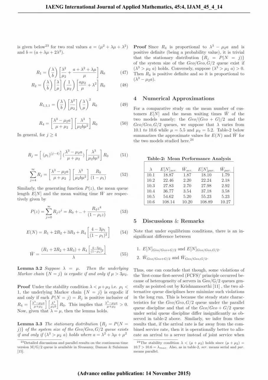
For a comparative study on the mean number of cus-tomers E[N ] and the mean waiting times W̄ of thetwo models namely; the Geo/(Geo + G)/2 and theGeo/Geo,G/2 queues, we suppose that λ varies from10.1 to 10.6 while μ = 5.5 and μ2 = 5.2. Table-2 belowsummarizes the approximate values for E(N) and W̄ forthe two models studied here.24

Table-2: Mean Performance Analysis

λ E[N ]ser. W̄ser. E[N ]par. W̄par.

10.1 18.87 1.87 18.10 1.7910.2 22.46 2.20 22.24 2.1810.3 27.83 2.70 27.98 2.9210.4 36.77 3.54 37.18 3.5810.5 54.62 5.20 55.23 5.2310.6 108.14 10.20 108.89 10.27

5 Discussions & Remarks

Note that under equilibrium conditions, there is an in-significant difference between

1. E[N ]Geo/Geo+G/2 and E[N ]Geo/Geo,G/2.

2. W̄Geo/Geo+G/2 and W̄Geo/Geo,G/2.

Thus, one can conclude that though, some violations ofthe ’first-come first-served (FCFS)’ principle occurred be-cause of heterogeneity of servers in Geo/G/2 queues gen-erally as pointed out by Krishnamoorthi [11] , the two al-ternative queue disciplines here minimize such violationsin the long run. This is because the steady state charac-teristics for the Geo/Geo,G/2 queue under the parallelqueue discipline and that of the Geo/Geo + G/2 queueunder serial queue discipline differ insignificantly as ob-served in table-2 above. Similarly, we infer from theseresults that, if the arrival rate is far away from the com-bined service rate, then it is operationally better to allo-cate an arrival to a server instead of joint service when

24The stability condition λ < (μ + μ2) holds since (μ + μ2) =10.7 > 10.6 = λmax. Also, as in table-2, ser . means serial and par .means parallel.



______________________________________________________________________________________

another arrival is present. As can be seen in the table-2above where in this case both the mean queue length andthe waiting time of the model under the parallel queuediscipline is stationary smaller than that of the model un-der serial service. However, the serial queue discipline isa better alternative especially in high-speed service sys-tems with arrival rates approaching the combined servicerates.

The results obtained in this work can be applied in ser-vice systems where customer distribution is required forbetter practice. Comparing the model with similar onesdiscussed in the literature, the ones here are simpler andresults compact, hence a good alternative for use. Mostimportantly is the new result of our work that under theserial queue discipline applied on the two-serially con-nected servers as in the Geo/Geo+G/2 and the parallelqueue discipline applied when the servers are in paral-lel as in the Geo/Geo,G/2 queue, the Geo/Geo + G/2and Geo/Geo,G/2 models are identical if and only ifλ3 > μ2(μ

2 + λμ + λ2). This ensures that the associ-ated Markov chain for the arrival distribution is ergodic.

There is a scope in studying the models discussed herevia Markov-renewal theory as in Senthamaraikannan andSivasamy [14].

The importance of control in the design and analysis ofmodels of service systems cannot be over emphasized.For a detail discussion, see Mohammad & Ali [13]. Re-cently, Sulaiman & Daman [16] have presented an exactanalysis of both the arrival distribution and waiting timeexpectation for a continuous time M/G/2 queuing systemworking under a control queue discipline.25 The analysisshows that the M/G/2 queue with the embedded controlperforms better than the continuous time M/G/2 queueunder both the serial and the parallel queue disciplines.Under similar assumptions employed for the model withcontrol, we conjectured that

Conjecture 1 Under heavy traffic conditions, theGeo/G(control)/2 model will perform better than theGeo/G/2 queues studied in this work.

Acknowledgment: This work has been supported bythe authorities of University of Botswana.

Appendices

Appendix AIf Rj = P [N = j] is the probability that there are jarrivals in the system, then

R0 = P [N = 0] = R0,0

R1 = P [N = 1] = R1,0 +R0,1

25Details of this queue discipline is found in Sulaiman & Daman[16].

R2 = P [N = 2] = R1,1,0 +R1,1

R3 = P [N = 3] = R1,1,1

Rj = P (N = j); j = 4, j = 5, ....,

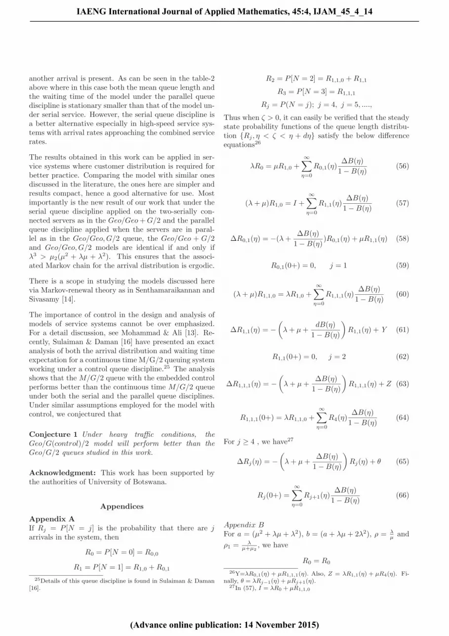
Thus when ζ > 0, it can easily be verified that the steadystate probability functions of the queue length distribu-tion {Rj , η < ζ < η + dη} satisfy the below differenceequations26

λR0 = μR1,0 +

∞∑η=0

R0,1(η)ΔB(η)

1−B(η)(56)

(λ+ μ)R1,0 = I +

∞∑η=0

R1,1(η)ΔB(η)

1−B(η)(57)

ΔR0,1(η) = −(λ+ΔB(η)

1−B(η))R0,1(η) + μR1,1(η) (58)

R0,1(0+) = 0, j = 1 (59)

(λ+ μ)R1,1,0 = λR1,0 +

∞∑η=0

R1,1,1(η)ΔB(η)

1−B(η)(60)

ΔR1,1(η) = −(λ+ μ+

dB(η)

1−B(η)

)R1,1(η) +Y (61)

R1,1(0+) = 0, j = 2 (62)

ΔR1,1,1(η) = −(λ+ μ+

ΔB(η)

1−B(η)

)R1,1,1(η) + Z (63)

R1,1,1(0+) = λR1,1,0 +

∞∑η=0

R4(η)ΔB(η)

1−B(η)(64)

For j ≥ 4 , we have27

ΔRj(η) = −(λ+ μ+

ΔB(η)

1−B(η)

)Rj(η) + θ (65)

Rj(0+) =

∞∑η=0

Rj+1(η)ΔB(η)

1−B(η)(66)

Appendix BFor a = (μ2 + λμ + λ2), b = (a + λμ + 2λ2), ρ = λ

μ and

ρ1 = λμ+μ2

, we have

R0 = R0

26Y=λR0,1(η) + μR1,1,1(η). Also, Z = λR1,1(η) + μR4(η). Fi-nally, θ = λRj−1(η) + μRj+1(η).

27In (57), I = λR0 + μR1,1,0



______________________________________________________________________________________

R1,1 = ρR0,1

R1,0 =

[μ2

λ

(λ2 + λμ+ a

λμ

)]R0,1 (67)

R1,1,0 =

[[μ2

λ

]( a

μ2

)]R0,1 (68)

R0,1 =

[λ3

μ2[a+ 2λ2 + λμ]

]R0 (69)

R2 =

[λ2

μμ2[a+ 2λ2 + λμ]

(a

μ+ λ2

)]R0 (70)

R1,1,1 =

(λ

μ

)2 [λ3

μ2[a+ 2λ2 + λμ]

]R0 (71)

R4 =

[λ3 − μ2a

μ+ μ2

] [λ3

μ2[a+ 2λ2 + λμ]

]R0 (72)

References

[1] Artalejo, J.R., & Lopez-Hererro, M.J., A Simulationstudy of a Discrete-Time Multiserver Retrial Queuewith Finite Population, Journal of Statistical Plan-ning and Inference, 137, 2536-2542, 2007.

[2] Boxma, O.J., Deng, Q., & Zwart, A.P., Waiting timeasymtotics for the M/G/2 queue with heterogeneousservers, Queuing Systems, 40, 5-31, 2002.

[3] Briem, U., Theimer, T.H., & Kroner, H., A GeneralDiscrete-Time Queuing Model: Analysis and Appli-cations, International Teletraffic Congress ITC-13,14, 13-19, 1991.

[4] Bruneel, H., Performance of Discrete-Time QueuingSystems, Computers in Operations Research, 20(3),303-320, 1993.

[5] Bruneel, H., & Kim, B.G., Discrete time modelsfor communication systems including ATM, KluwerAcademic Publishers, Norwell, MA, 1999.

[6] Bruneel, H., Walraevens, J., Claeys, D., & Wit-tevrongel, S., Analysis of a Discrete-Time Queuewith Geometrically Distributed Service Capaci-ties, LNCS 7314, Springer-Verlag-Berlin- Heidel-berg, 121135, 2012.

[7] Goswami, V., Analysis of discrete-time multi-server queue with balking, International Journal ofManagement Science and Engineering Management,9(1), 21-32, 2013.

[8] Goswami, V., & Mund, G.B., Multiserver bulk ser-vice discrete-time queue with finite buffer and re-newal input, Computers and Mathematics with Ap-plications, 57, 1377-1388, 2009.

[9] Gupta, U.C., & Goswami, V., Performance analysisof finite buffer discrete-time queue with bulk service,Computers & Operations Research, 29, 1331-1341,2002.

[10] Ishizaki, F., Takine, T., & Hasegawa, T., Analysisof a Discrete-Time Queue with geometrically Dis-tributed Gate Opening Intervals, Journal of theOperations Research Society of Japan, 39(1), 1-24,1996.

[11] Krishnamoorthi, B., On Poisson Queue with twoHeterogeneous Servers, Operations Research, 2(3),321-330, 1963.

[12] Mirtchev, S., & Goleva, R., Discrete-Time Singleserver model with a Multimodal packet size distri-bution, Proceedings of a Conjoint Seminar in Mod-eling and Control of Information Processes, Sofia,Bulgaria, CTP, Sofia, 83-101, 2009.

[13] Mohammad, K. & Ali, M., A Hybrid Method forSolving Optimal Control Problems, IAENG Inter-national Journal of Applied Mathematics, 42(2), 80-86, 2012.

[14] Senthamaraikannan, K., & Sivasamy, R., EmbeddedProcesses of a Markov Renewal Bulk Service Queue,Asia Pacific Journal of Operational Research, 11(1),51-65, 1997.

[15] Sivasamy, R., Daman, O.A., & Sulaiman, S., AnM/G/2 Queue where Customers are Served subjectto a Minimum Violation of the FCFS Queue Dis-cipline, European Journal of Operational Research,240, 140146, 2014.

[16] Sulaiman, S., & Daman, O.A., An M/G/2 Queuewith Heterogeneous Servers working Under a Con-trol Service Schedule: Stationary Performance Anal-ysis. IAENG International Journal of Applied Math-ematics, 45(1), 21-30, 2015.

[17] Takagi, H., Queuing Analysis: A Foundation ofPerformance Evaluation in Discrete-Time systems,Volume 3, North-Holland Publishing, Amsterdam,1993.



______________________________________________________________________________________

Documents

Discrete-Time Geo/G/2 Queue under a Serial and Parallel Queue Disciplines