Embed Size (px)
Citation preview

157
4Displacement Measuring Interferometry
Vivek G. Badami and Peter J. de Groot
CONTENTS
4.1 Introduction ........................................................................................................................ 1584.2 Fundamentals ..................................................................................................................... 1594.3 Phase Detection .................................................................................................................. 1614.4 Light Sources for Heterodyne Displacement Interferometry ...................................... 164
4.4.1 Zeeman-Stabilized Lasers .................................................................................... 1664.4.2 Polarization-Stabilized Lasers ............................................................................. 1684.4.3 Stabilization Using Saturated Absorption:
Iodine-Stabilized He-Ne Laser ........................................................................... 1704.5 Interferometer Design ....................................................................................................... 1734.6 Error Sources and Uncertainty in DMI .......................................................................... 178
4.6.1 Uncertainty Sources .............................................................................................. 1804.6.2 Vacuum Wavelength.............................................................................................. 1814.6.3 Refractive Index ..................................................................................................... 1824.6.4 Air Turbulence........................................................................................................ 1854.6.5 Cosine Error ............................................................................................................ 1864.6.6 Phase Measurement .............................................................................................. 1874.6.7 Cyclic Errors ........................................................................................................... 1884.6.8 Deadpath ................................................................................................................. 1914.6.9 Abbe Error............................................................................................................... 1934.6.10 Optics Thermal Drift ............................................................................................. 1964.6.11 Beam Shear ............................................................................................................. 1964.6.12 Target Contributions ............................................................................................. 1974.6.13 Data Age Uncertainty ............................................................................................ 1984.6.14 Mounting Effects .................................................................................................... 198
4.7 Applications of Displacement Interferometry ............................................................... 1994.7.1 Primary Feedback Applications .......................................................................... 199
4.7.1.1 High-Accuracy Machines ...................................................................... 1994.7.2 Angle Measurement .............................................................................................. 2024.7.3 Measuring Machines ............................................................................................. 2044.7.4 Very High Precision ............................................................................................... 2104.7.5 Reference or Validation Metrology ..................................................................... 210
4.8 Alternative Technologies .................................................................................................. 2144.8.1 Absolute Distance Interferometry ....................................................................... 2144.8.2 Optical Feedback Interferometry ........................................................................ 2164.8.3 Dispersion Interferometry .................................................................................... 217

158 Handbook of Optical Dimensional Metrology
4.1 Introduction
The wavelength of light provides an exceedingly precise measure of distance and is the foundation for commercial interferometric measurement tools that monitor object posi-tions with a resolution better than 1 nm for objects traveling at 2 m/s. A wide range of applications include machine tool stage positioning and distance monitoring over length scales from a few millimeters to hundreds of kilometers in space-based systems.
Displacement measuring interferometry or DMI enjoys multiple advantages with respect to other methods of position monitoring. In addition to high resolution, wide measure-ment range, and fast response, the laser beam for a DMI is a virtual axis of measurement that can pass directly through the measurement point of interest (POI) to eliminate Abbe offset errors. Figure 4.1 illustrates the position of DMI in terms of resolution and dynamic range with respect to capacitive gaging, optical encoders, and linear variable differential transformer (LVDT) methods. The measurement is noncontact and directly traceable to the unit of length. Since the first practical demonstration of automated, submicron stage control using displacement interferometry in the 1950s,1 DMI has played a dominant role in high-precision positioning systems.
This chapter is intended as an overview of the current state of the art in DMI as repre-sented by the technical and patent literature. The chapter structure is correspondingly encyclopedic and allows for access to specific topics without necessarily reading the chapter linearly from start to finish.
Following this brief introduction, we begin in Section 4.2 with fundamental physical principles of DMI, followed in Section 4.3 by a review of phase detection methods most
4.8.4 Optical Fibers and DMI ........................................................................................ 2184.8.5 Optical Encoders .................................................................................................... 220
4.9 Summary: Using Displacement Interferometry ............................................................ 221References .....................................................................................................................................222
10–5
10–10
10–9
10–8
10–7
10–6
10–4 10–3 10–2
Maximum range (m)
Reso
lutio
n (m
)
DMI
EncodersLVDT
Capaci
tance
gages
10–1 100 101 102
FIGURE 4.1DMI with respect to comparable devices for distance measurement.

159Displacement Measuring Interferometry
common in practical implementations, introducing the essential concepts of homodyne and heterodyne detection. Section 4.4 considers ways of generating wavelength-stable light having the coherence and modulation characteristics essential for heterodyne DMI. Section 4.5 catalogs some of the more common optical interferometer configurations sensitive to various measurement parameters such as displacement, angle, and refractive index. With these tools in hand, we then examine in Section 4.6 the question of system performance in terms of the measurement uncertainty, encompassing error sources such as wavelength instability, Abbe offset error, cyclic error, air turbulence, and thermal drift. A gallery of practical DMI applications follows in Section 4.7, considering calibration and validation tasks as well as integration of DMI into a complete machine for continuous motion control and/or measurement. The applications section includes examples of unusual technology approaches that may find more common usage going forward.
4.2 Fundamentals
The high precision of DMI leverages the rapid change of phase as light propagates, equiva-lent to a 2π phase shift for a distance of less than half a micron for visible light. This fine-scale, traceable metric is accessible through interferometric methods of comparing reference and measurement beams generated from a common source light beam and then recombined.
To establish terminology and notation, we provide here a mathematical description of the principles of the technique. The oscillating electric field of a source beam of ampli-tude E0 is
E t z E i ft nz( , ) exp= −
0 2π
λ (4.1)
wheref is the frequency of oscillationλ is the vacuum wavelengthz is the physical path lengthn is the index of refraction
The frequency at visible wavelengths is very high—approximately 6 × 10¹⁴ Hz—making it difficult to detect the phase 2π( ft − nz/λ) of E(t, z) directly. To access the wavelength as a unit of measurement, we need to remove or at least drastically slow down the optical fre-quency component. This is why we use interferometry.
Referring to Figure 4.2, the nonpolarizing beam splitter (NPBS) splits the source light into two beams, labeled 1 and 2 for the measurement and reference beams, respectively. These beams follow different paths and therefore have different phase offsets related to the propagation term nz/λ:
E t z r E ift i nz
1 1 1 012 2( , ) exp( )exp= −
π πλ
(4.2)

160 Handbook of Optical Dimensional Metrology
E t z r E ift i nz
2 2 2 022 2( , ) exp( )exp= −
π πλ
(4.3)
wherez1, z2 are the path lengths traversed by beams from the point that they are separated by
the NPBS to the point that they are recombinedr1, r2 are their relative strengths with respect to the original complex amplitude |E0|
When the two beams superimpose coherently on a square-law detector, the time average of the resulting intensity is
I z z E ift r i nz r i nz( ) exp( ) exp exp1 2 0
2 21
12
22 2 2= −
+ −
π πλ
πλ
2
(4.4)
The frequency term ft averaged over time becomes a constant:
exp( )2 12πift = (4.5)
but the final expression preserves the optical path difference z1 − z2:
I L I I I I L( ) cos[ ( )]= + +1 2 1 2 φ (4.6)
where
I r E1 1 02= (4.7)
I r E2 2 02= (4.8)
Non polarizingbeam splitter
(NPBS)
To detector
From source
Referencebeam (2)
Measurementbeam (1)
L
Referencemirror
Objectmirror
FIGURE 4.2Michelson-type amplitude division interferometer for monitoring the position of an object mirror.

161Displacement Measuring Interferometry
φ π
λ( )L nL=
4 (4.9)
2 1 2L z z= − (4.10)
The fundamental principle of DMI is to detect changes in the distance L by evaluation of the interference phase ϕ(L) via its effect on the time-averaged intensity I(L).
4.3 Phase Detection
As is the case with all forms of interferometry, there is a heavy emphasis in DMI technol-ogy development on methods of determining the phase ϕ(L). In the earliest interferom-eters, dating back to Michelson, phase estimation was visual.2,3 The visual method relies on the presence of a spatial fringe pattern viewed by the eye, generated, for example, by tilting one of the interferometer mirrors. The experienced observer with the aid of a crosswire or adjustable compensating optical element can estimate to about 1/40 th of a fringe or 15 nm—sufficient for routine gage block measurements.4,5 Another historical technique especially useful for objects in motion is fringe counting—essentially keep-ing a tally of the number of times that the output beam goes from light to dark—which is appropriate for low-precision applications for which a displacement estimate with a resolution of λ/2 is sufficient and for which there is no uncertainty regarding the direc-tion of motion.
Modern DMI systems rely on electronic detection and data processing to allow for an evaluation of the intensity over a range of controlled phase shifts to establish the direction of motion and to interpolate to small fractions of a fringe. In the majority of systems, this means encoding the reference and measurement beams by polarization, so that they can be mixed with three or more phase shifts α between them:6
I L I I I I L( , ) cos[ ( ) ]α φ φ α= + + + +1 2 1 2 0 (4.11)
A sequence of phase shifts allows for signal processing based on quadrature detection, the fitting of sines and cosines, or equivalent methods to solve for ϕ(L). The additional phase term ϕ0 is a constant offset equal to the detected phase for the displacement position defined as L = 0.
Figure 4.3 illustrates one arrangement for encoding the reference and measurement beams by polarization. A polarizing beam splitter (PBS) separates source light into a ref-erence and a measurement beam according to s and p linear polarizations, respectively. A suitable source polarization would be linear, at a 45° angle with respect to the plane of the figure. Reference and object corner cubes reverse the beam paths so that they are col-linear and aligned parallel when recombined by the PBS.7 This exit beam now contains the reference and measurement beams encoded by orthogonal linear polarizations.
Two established options for phase detection with polarization-encoded interferometers are the homodyne and heterodyne techniques.

162 Handbook of Optical Dimensional Metrology
In the homodyne method, polarizing optics and multiple detectors measure the inten-sity for several static phase shifts imposed by polarizing optics.8 Figure 4.4 illustrates an example homodyne detector employing quarter-wave and half-wave retardation plates (QWP and HWP, respectively). The four detectors shown in the figure detect intensity signals with π/2 relative phase shifts:
I I Lj j= ( , )α (4.12)
α π
jj=2
(4.13)
Polarizingbeam splitter
(PBS)
Referenceretroreflector
L
Objectretroreflector
From source
To phase detector
s polarizationp polarization
FIGURE 4.3Linear displacement interferometer using retroreflectors and polarization encoding of the measurement and reference beams.
From interferometer
QWP to introduce45° phase shift
HWP plate to rotate polarization 45°
Detector 1
Detector 3
Detector 4
Detector 2
PBS
NPBSPBS
FIGURE 4.4Optical components of a homodyne phase detector.

163Displacement Measuring Interferometry
The phase follows (to within a constant offset) from the formula
tan( )φ = −
−I II I
1 3
2 4
(4.14)
This method is to first order insensitive to fluctuations in the source intensity and fringe contrast and, to the degree that the imperfections in the detection optics can be compen-sated algorithmically9 or by design,10 provides a precise estimate of the instantaneous phase and the displacement L. Homodyne detection is popular for low-cost, single-axis DMI systems11,12 and for optical encoders.13 Variations include reversing the roles of the wave plates in Figure 4.4 or creating a spatial pattern of interference fringes by recombin-ing the measurement and reference beams at a small angle, similar to what was done in the earliest days of interferometry, with fixed sampling points at different points on a fringe.14
In the heterodyne method, the interference intensity is continuously shifted in phase with time by imparting a frequency difference between the reference and measurement beams.15–17 Instead of sharing a common optical frequency f, an offset frequency Δf = f2 − f1 is imposed between reference and measurement beams, usually at the source, resulting in a continuous, time-dependent phase shift in Equation 4.11:
α( )t ft= ∆ (4.15)
The output beam intensity varies sinusoidally at a rate of a few kilohertz to hundreds of megahertz, depending on the system design and the anticipated maximum object velocity. A single detector captures this signal for each measurement direction or axis (Figure 4.5). Several different ways are available to analyze this signal, including lock-in methods, zero crossing, and sliding-window Fourier analysis, with advanced data age compensation for high-speed servo control.18 Often there is an electronic reference sig-nal, generated either electronically from the drive electronics that generate the frequency shift Δ f or optoelectronically, by measuring the phase of the heterodyne signal detected prior to the interferometer optics.
Measurement beam,at frequency f1
Frominterferometer
Reference beam,at frequency f2
Fiber-optic pickup(FOP)
Mixing polarizerat 45°
Multimodeopticalfiber
Detector
SignalI
t
FIGURE 4.5Heterodyne detection using a fiber-optic pickup (FOP).

164 Handbook of Optical Dimensional Metrology
Of the several advantages of heterodyne systems, we note the simplicity of the detector, which is particularly important in cost-effective multiaxis systems, and the shifting of the signal to a frequency far from DC to avoid thermal and other statistical noise sources that scale inversely with frequency. The various components of a heterodyne interferometer system shown in Figure 4.6 address a wide variety of measurement configurations. In particular, heterodyne interferometry serves high-precision applications such as micro-lithographic staging (see Section 4.7).
4.4 Light Sources for Heterodyne Displacement Interferometry
Light sources for heterodyne interferometry must satisfy multiple optical and met-rological requirements. They generate two linear-polarized mutually orthogonal frequency-shifted beams at a stable and known wavelength. The last two requirements also establish traceability to the unit of length and provide the scaling factor required to convert the change in phase measured at the output of the interferometer into units of length. Common applications also require coherence lengths of the order of meters, although sources with short coherence lengths may be used to advantage in some appli-cations.19,20 Additional practical demands include compact size, low heat dissipation, high optical output power, high level of stability of the pointing and polarization state orientation relative to a mechanical datum, optical isolation from reflected beams, and high wavefront quality.
Laser sources, especially gas laser sources, satisfy virtually all of the requirements. One of the earliest two-frequency lasers to be applied to displacement interferometry was a modified helium–neon (He-Ne) gas laser15 shortly after continuous-wave emission at 632.9 nm was demonstrated in 1962.21 Although specialized applications use other laser types and wavelengths22,23 and a number of light sources provide a practical realiza-tion of the meter,24 the He-Ne laser operating at 632.9 nm remains the laser of choice for
Opticalfibers
Interferometer
Laser sourceElectronics
Objectmirror
FIGURE 4.6Components of a heterodyne laser system. (Photo courtesy of Zygo Corporation, Middlefield, CT.)

165Displacement Measuring Interferometry
metrology applications. This preference stems from a number of reasons, including inher-ent simplicity, ease of alignment due to the visible radiation, and the ready availability of silicon photodetectors.25 The following discussion confines itself to this type of laser and in particular to the commonly available commercial implementations and the stabilization schemes used therein.
The value of wavelength of the He-Ne laser and the associated uncertainty are key parameters in DMI. The value of the vacuum wavelength (along with the refractive index) scales the measured phase changes into units of length, and any uncertainty in the wave-length propagates directly into the uncertainty in the displacement measurement (see Section 4.6). The basic atomic physics of the He-Ne laser operating at a vacuum wavelength of 632.9 nm (3s2 → 2p4 transition in neon) has interesting implications for the realization of the unit of length in that the atomic transition is a reliable optical standard of wavelength, albeit with an associated uncertainty.26 As shown in Figure 4.7, the width of the gain curve above the threshold is ∼1.4 GHz (or 3 × 10⁻⁶ in terms of relative frequency) and is deter-mined by the governing physics of this type of laser. A recent recommendation of the Consultative Committee for Length (CCL) of the International Committee for Weights and Measures (CIPM) has resulted in the inclusion of the unstabilized He-Ne laser operating at 632.9 nm in the list of light sources used to realize the unit of length.27 The CIPM rec-ommended value of the associated relative standard uncertainty is 1.5 × 10⁻⁶, which with a coverage factor of two exceeds the width of the gain curve above threshold. Although this establishes some degree of traceability for a free-running He-Ne laser, the 1.5 × 10⁻⁶ level of uncertainty is insufficient for many DMI applications, and stabilization of the laser wavelength is a necessity.
Figure 4.8 represents a classification of He-Ne laser sources for heterodyne DMI based on the method used to stabilize them. Dual-frequency lasers (hereafter referred to as metrology lasers) are for use in heterodyne DMI systems. Reference lasers in the right-hand branch of Figure 4.8, such as the 127
2I -stabilized He-Ne laser, realize the definition of the meter to very high levels of accuracy for calibration of metrology lasers when used in accordance with the recommendations of the BIPM.24 The majority of commercial DMI laser systems follow the left-hand branch of Figure 4.8 and use a single emission mode for
Threshold
f= 473.6127 THzλ = 632.9908 nm
~1.4 GHz
FIGURE 4.7Gain curve of the He-Ne laser at ∼633 nm. Frequency and wavelength are the CIPM recommended values. (From Stone, J.A. et al., Metrologia, 46, 11, 2009.)

166 Handbook of Optical Dimensional Metrology
metrology, although they may operate multimode for the purpose of stabilization by refer-ence to the gain curve. A minority of these lasers use two or more lasing modes directly, with the heterodyne frequency established by the difference in optical frequency between these modes.28–30
Commercial metrology lasers are stabilized by controlling the position of two orthog-onally polarized TEM00 modes relative to the gain curve for the He-Ne gain medium. Adjustment of the length of the resonator under closed-loop control drives the differ-ence in intensities of the two modes to zero. Two methods effect gain-curve stabilization: Zeeman splitting and polarization stabilization.
4.4.1 Zeeman-Stabilized Lasers
The Zeeman laser31–33 traces its roots to the devices described by Tobias et al.34 and by de Lang et al.15 The method relies on the Zeeman effect,35 wherein the application of a relatively strong magnetic field along the axis of the tube results in a “splitting” of the single laser mode into two orthogonally circularly polarized modes as depicted in Figure 4.9, with frequencies slightly above and below the original center frequency f0, denoted by f+ and f−, respectively. Zeeman splitting provides the frequency difference required for heterodyne interferometry as well as a method for stabilization of the laser wavelength. The frequency difference depends on the magnitude of the applied mag-netic field and ranges from about 1 to 4 MHz. While commercial laser sources rely on a strong axial magnetic field to produce the two modes, alternate implementations using a transverse magnetic field have also been reported in the literature.36–38
Figure 4.10 shows a schematic of a typical Zeeman-split laser source. The internal cavity He-Ne laser operates at a single longitudinal and lateral mode at ∼633 nm. The require-ment for single-mode operation dictates the maximum length of the resonator cavity,
Two and threemode
Stabilized He-Nelaser sources at
~633 nm
Saturatedabsorptionstabilized
Lamb dipstabilized
Zeemanstabilized
Polarizationstabilized
Strong axialmagnetic
field
Weak axialmagnetic
field
Dual-frequency metrology sources
Transversemagnetic
fieldWavelength
reference sources
127I2 Stabilized
Gain curvestabilized
FIGURE 4.8Classification of laser sources. Dashed lines indicate sources that are restricted to laboratory use or in limited commercial use.

167Displacement Measuring Interferometry
which in turn sets an upper bound on the achievable power. Permanent magnets that surround the laser tube apply an axial magnetic field. A beam splitter (BS) samples a small portion of the two orthogonal circularly polarized beams exiting the tube for sta-bilization. The two circularly polarized states convert to orthogonal linearly polarized states that generate an error signal for the feedback system that controls the length of the laser cavity. Typical commercial implementations separate the two linearly polarized beams and direct them onto two detectors and use the difference in the outputs as the error signal.31,33 An alternative method that eliminates the need to match the detector gains employs a single detector and a programmable liquid-crystal polarization rotator to alternately sample the intensities of the two polarizations.33 The intensity difference between the two modes as a function of resonator length exhibits a zero crossing with a large slope at the point corresponding to the unshifted center frequency. This slope makes it possible to stabilize the wavelength by controlling the length of the resonator using either a piezoelectric (PZT) actuator15,31 or a heating element.33 An alternate method uses
LCP RCP
~2 MHz
f– f+f0
Threshold
FIGURE 4.9Splitting of single longitudinal laser mode into two orthogonal polarization states (left circular polarized or LCP and right circular polarized or RCP) due to Zeeman splitting. The split is exaggerated for clarity.
Polarizationseparation optics
Axial magnetic field
Controller
Circular linearpolarizations
Orthogonallinear
polarizationsQWP
MirrorMirror
Heaterelement
Polarizationseparation optics
Permanent magnetsBS
Intensitycomparison
f–
f–
f+
f+
FIGURE 4.10Schematic representation of a Zeeman-stabilized laser.

168 Handbook of Optical Dimensional Metrology
the beat frequency between the two modes,32 obtained by arranging for the two beams to interfere by means of a linear polarizer prior to directing them onto a single detector. Locating the minimum in the beat frequency as function of resonator length controls the resonator length.
As shown in Figure 4.10 by the dashed lines, the laser output for stabilization can be the weaker beam that exits the rear of the tube, thereby making all of the main output of the laser available to the metrology application. A recent design exploits the elliptically polarized beams that result from the inherent anisotropy in the laser tube to produce the feedback signal without any additional polarization optics.39,40 The light exiting the source transforms into two mutually orthogonal linearly polarized beams (at two slightly different frequencies) by means of a QWP. In this type of laser, the production of the two frequencies for heterodyne DMI is integral to the stabilization scheme.
While the Zeeman method has some drawbacks from a control standpoint,41 Hewlett–Packard (now Agilent),31,33 Zygo Corporation,42 and other manufacturers produce Zeeman laser DMI systems that have played a significant and widespread role in metrology. A drawback of this method is the low heterodyne frequency and the resulting limitation on the maximum slew rate of the target. A further drawback is the requirement on single-mode operation of the tube,43,44 which limits the length of the laser tube to less than about 10 cm and in turn reduces the achievable output power compared to the longer tubes used in polarization-stabilized lasers.
The quality of the exiting beams in terms of the orthogonality and ellipticity are key parameters that have an impact on the cyclic errors, as described in Section 4.6. Early char-acterizations of these parameters report deviations from orthogonality of 4°–7°,45 while more recent measurements suggest a much smaller value of 0.3° and an ellipticity of 1:170 in the electric field strength.46
4.4.2 Polarization-Stabilized Lasers
In contrast to the Zeeman-stabilized system, polarization-stabilized DMI laser source sys-tems separate the stabilization and frequency shifting functions.17,47–49 The stabilization technique relies on matching the intensities of two adjacent longitudinal modes as shown in Figure 4.11.50,51 The presence of two orthogonally polarized modes under the gain curve
Threshold
474 THz
640 MHz
~1.4 GHzLinear
orthogonallypolarized
modes
fk fk+ 1
FIGURE 4.11Two-mode operation of a polarization-stabilized laser.

169Displacement Measuring Interferometry
makes it possible for the tube in a polarization-stabilized laser to be longer than in the Zeeman-stabilized laser (∼30 cm).
A BS as shown in Figure 4.12 samples a small portion of the output beam. A Wollaston prism (or other suitable birefringent prism) divides the sampled beam according to the two orthogonal polarizations corresponding to the two lasing modes and directs them on to two detectors D1 and D2.50 The control system strives to minimize the difference in intensity observed at the two detectors D1 and D2 by adjusting the cavity length. As shown in Figure 4.11, which depicts the relative intensities of the modes when the laser is in the stabilized condition, the two modes are disposed symmetrically with respect to the wave-length corresponding to the peak of the gain curve.
The polarizer following the BS passes only one of the modes, which then passes through an acousto-optic modulator (AOM) to produce the two mutually orthogonal linearly polar-ized frequency-shifted beams arranged to overlap and emerge parallel to one another from the laser by using a second birefringent prism (not shown).47 The frequency difference Δf corresponds to the drive frequency of the AOM. Although one of the modes is rejected, the increase in tube length (when compared to a Zeeman-stabilized laser) for two-mode operation more than makes up for the loss of one of the modes, resulting in a net gain in output power. This method of frequency shifting allows for large frequency differences relative to the Zeeman frequency split, with a 20 MHz frequency difference being com-mon, which supports much higher slew rates of the target. This technique is however less efficient in its use of the available light. One way to recover the lost power is to use the two lasing modes to supply two independent interferometers.52
Commercial-stabilized laser sources typically specify a relative “vacuum wavelength accuracy” or “unit-to-unit variability” of ±0.1–0.8 × 10−6.42,52,53 These numbers can be the basis for the estimation of a standard uncertainty in the vacuum wavelength. If a more accurate value of the wavelength is desired, the wavelength should be determined for the source in question by comparison against an iodine-stabilized He-Ne laser 41,54 or against a frequency comb.55 Stabilities for commercial sources are typically specified over various time scales, with short-term (1 h), medium-term (24 h), and long-term (over the laser life-time) relative wavelength stabilities of ±0.5–2 × 10⁻⁹, ±1–10 × 10−9, and ±10–20 × 10−9, respec-tively.53,56 A recent report on the measurement of 28 different laser heads of both types by
Laser tube
Controller
+–
Heater element MirrorMirror BS Polarizer
AOM
D1
D2
∆f
f
f1 = f+ ∆f
f2 = f
Birefringentprism
FIGURE 4.12Schematic of a polarization-stabilized laser.

170 Handbook of Optical Dimensional Metrology
comparison to an iodine-stabilized He-Ne laser over a period of 20 years confirms that in general the manufacturer’s specifications are met or exceeded.57
Some special care is necessary to achieve the stated stability of the laser. One cause for degradation in laser stability is optical feedback caused by reflections back into the laser cavity from external sources.58,59 Even weak reflections of ∼0.01% of the output of the laser can cause major instabilities in older systems resulting from the formation of unstable external cavities outside the influence of the stabilization control.43,58 Traditional methods to combat optical feedback include rotating the polarization of the reflected beam in a nonreciprocal manner by means of a Faraday cell so as to prevent reentry of the reflected beam into the resonator by means of a crossed polarizer.60
Using an AOM to generate the two frequencies provides an inherently high degree of feedback isolation.47,61 Beams reflected back through the laser system are either directed away from their original beam paths or are frequency shifted outside the gain bandwidth of the laser.41,62 Some modern systems have further enhanced isolation by specialized AOM design, effectively eliminating optical feedback as a source of concern.52,63
General considerations common to all types of laser heads include beam size, heat dis-sipation, pointing stability, and other operational characteristics.
The beam is typically expanded by means of a telescope (not shown) to above 5 mm diameter so as to limit the natural beam divergence that results from Gaussian beam propagation and permit measurements over reasonable displacement ranges.64 Another consideration that dictates the beam size is tolerance to shear between the measurement and reference beams. Lateral translations and angular misalignments of the measurement beam relative to the reference beam can result from errors in the optics and alignment, and the beam size must provide adequate overlap.65 Commercial systems most commonly produce a beam with a 6 mm 1/e2 diameter, which offers a reasonable trade-off between measurement range and the size of the interferometer optics; 53,56,66,67 although 3 and 9 mm beam diameters are available as options.53
Heat dissipation by the laser head is a thermal management issue in demanding appli-cations. Laser heads typically dissipate 20–40 W during operation and must be carefully located to minimize the heat load.53,56 Specialized heads use liquid cooling to reduce the dissipated power to under 10 W.66,67 Another option is to locate the head remotely and couple the light into the application via optical fibers.66
4.4.3 Stabilization Using Saturated Absorption: Iodine-Stabilized He-Ne Laser
Lasers stabilized by saturated absorption provide the highest level of stability and repro-ducibility in the field of dimensional metrology and are typically used by National Metrology Institutes (NMIs) as the primary means to realize the unit of length.68 These sin-gle-frequency lasers represented by the right branch of Figure 4.8 calibrate two frequency metrology lasers. The 633 nm iodine (I2)-stabilized He-Ne developed in the early 1970s remains the most common primary standard laser for dimensional metrology, largely because of the ease of calibration, achieved by mixing the output of the He-Ne metrology laser with the I2-stabilized laser emission and directly measuring the resulting radio fre-quency beat signal.
The vastly superior performance of the absorption-stabilized laser stems from the sepa-ration of the light generation and stabilization functions, making it possible to use a transi-tion in separate species as a reference. The stabilization subsystem is physically separate from the laser tube and can therefore be placed in a stable environment, uncoupling it from the perturbations that occur during the process of light generation (such as variations

171Displacement Measuring Interferometry
in pressure of the discharge tube). The separation results in improvements in the repro-ducibility of approximately 103.41
The I2 He-Ne relies on the saturation of absorption69 of the iodine cells to eliminate the Doppler broadening and make the hyperfine absorption lines in the iodine spectrum accessible. The absorption saturates because of the bidirectional standing waves within the cavity, resulting in a Lorentzian-shaped dip in the absorption of the iodine cell, the width of which corresponds closely to the natural line width of the transition and occurs at the center of the absorption line. This drop in the absorption of the cell results in sharp Doppler-free peaks with quality factors of ∼108 superimposed upon the Doppler-broadened gain curve of the He-Ne laser as shown in Figure 4.13a. These hyperfine lines are highly reproducible and relatively immune to perturbations,70 in large part because the hyperfine absorption lines are the result of transitions from the ground state, eliminating the perturbing influences of an excitation mechanism71 and guaranteeing a high level of wavelength reproducibility.
The gain in power at these peaks is typically ∼0.1% of the base output power at that wavelength, and any locking technique must be capable of recovering the weak signal from a strong background in order for the peak to serve as a frequency discriminator. The location of the peak is usually determined by the method of third-harmonic lock-ing that effectively determines the third derivative of the signal.71,72 This produces an
(a)
(b)
0
(c)
0
a b cd e f g h i j kl
mn
FIGURE 4.13(a) Gain curve of a cavity with a He-Ne plasma tube and iodine cell. (b) First and (c) third derivatives of the gain bandwidth curve with respect to frequency.

172 Handbook of Optical Dimensional Metrology
antisymmetric zero crossing at the location of the peak as shown in Figure 4.13c in contrast to the first derivative shown in Figure 4.13b, which does not always produce a zero cross-ing due to a large background slope.
Figure 4.14 shows a representative schematic of an iodine-stabilized He-Ne laser. While several different designs are available,70,71,73–80 virtually all implementations employ a DC voltage excited plasma tube that contains the He-Ne gas and a separate intracavity I2 cell, both of which have Brewster windows. The cell contains 127
2I at low pressure to reduce contributions of pressure broadening. A temperature-controlled cold-finger integral to the cell controls the pressure of the cell. Two high-reflectance mirrors (typically spherical) form the resonator cavity, and a PZT actuator displaces one or both in a controlled man-ner. To lock the laser frequency, a PZT actuator imposes a sinusoidal modulation on one of the cavity mirrors, and a photodetector senses the resulting modulation in the output. The third harmonic of the photodetector signal is phase sensitively demodulated against a ref-erence at the third harmonic of the modulation frequency. The resulting third-derivative signal serves as an error signal to a second PZT under closed-loop control that varies the length of the cavity and strives to drive the value of the third derivative to zero.
The CIPM specifies, through periodic publications, the nominal wavelength for a specific transition of the 127
2I He-Ne, the associated relative standard uncertainty, and the conditions required to achieve the stated uncertainty. The current recommendations adopted in 2001 specify a slightly revised value for the recommended frequency and a slightly reduced relative standard uncertainty of the wavelength of 2.1 × 10⁻¹¹ for the a16 or f component of the R(127) 11−5 transition for 127
2I based on measurements using frequency combs.24,81
Numerous international intercomparisons between He-Ne lasers and the iodine cells themselves have established the reproducibility of the 127
2I -stabilized He-Ne operating
Cavity mirrors
He-Ne plasma tube
Plasma tube HVsupply
Oscillator
3X frequencymultiplier
3f reference
1f1f modulation
3f phase sensitivedetector (PSD)
3f band-passfilter
Integrator PZT amplifier
Cooler
Tuning PZTModulation PZT
Detector
Prea
mpl
ifier
Iodine cell
Coldfinger
FIGURE 4.14Schematic of iodine-stabilized He-Ne laser.

173Displacement Measuring Interferometry
at 633 nm.82,83 Comparisons over a period of 25 years show that ∼85% of the lasers in the comparison agree to within the relative standard uncertainty of 2.5 × 10⁻¹¹ specified by the then current mise en pratique,84 and all the lasers were in agreement to within the relative expanded uncertainty with k = 3.85 Recent measurements of the frequency of these lasers by direct comparison to the second using femtosecond frequency combs show a reproduc-ibility of 1 × 10−12.86
Iodine-stabilized reference lasers typically operate with much lower output powers of approximately 100 μW and produce only a single, user-settable frequency, thereby making them unsuitable for direct use as a metrology laser in a heterodyne system.87 An additional limitation is that the output intensity of the laser modulates as a natural consequence of the small modulation imposed on one of the cavity mirrors as part of the third-harmonic locking scheme.88 In high-accuracy applications where the stability of the metrology laser is inadequate and/or uncertainty in the nominal wavelength is too large, embedding these lasers into the machine provides for continuous monitoring of the wavelength of the metrology laser.89,90 They may also be used as reference lasers for multiple higher-power metrology lasers, which are offset locked to the iodine-stabilized He-Ne, thereby produc-ing a source that combines the high stability of the iodine-stabilized laser with the higher unmodulated output power available from a conventional He-Ne.88,89,91
Table 4.1 provides an estimate of the relative accuracies and wavelength stabilities from manufacturer’s specification sheets for lasers without any special calibration. Data for the dual-frequency lasers use the manufacturer’s nomenclature, because of a lack of consis-tency in the method of specification. In contrast, at least one commercial iodine-stabilized laser specifies a relative standard uncertainty in the wavelength and specifies the stability in terms of the Allan variance as a function of time.87,92,93
4.5 Interferometer Design
Returning to the interferometer optics, the linear interferometer configuration of Figure 4.3 with retroreflectors serves well for applications that involve single-axis motion. The object retroreflector preserves the parallelism of the reference and measurement beams after recombination, even for small tilts of the object.7
TABLE 4.1
Relative Wavelength Accuracies and Stability of Stabilized He-Ne Lasers
Laser Type FrequencyRelative Wavelength
“Accuracy”
Wavelength Stability (×10−9)
1 h 24 h Lifetime
Zeeman stabilized
Dual Accuracy (3σ) ± 0.1 × 10⁻⁶ ±2 Not specified
±20
Polarization stabilized
Accuracy or unit-to-unit variability ± 0.1 – 0.8 × 10⁻⁶
±0.5a ±1a ±10a
Iodine stabilized Singleuc( ) .λ
λ= × −2 1 10 11 Allan variance of 10 11− t where t is the
measurement time
a 3σ values.

174 Handbook of Optical Dimensional Metrology
For dual-axis motion as required by an x–y stage, the preferred object is a plane mirror rather than a retroreflector. Figure 4.15 shows how this may be accomplished using a QWP. The QWP converts linear polarization to circular and then back to an orthogonal linear polarization after reflection from the object mirror, which is now free to move orthogonal to the line of sight without disturbing the beam paths. Figure 4.16 shows how the dou-ble pass to the object mirror with a retroreflection compensates for a tilt θ of the mirror. An additional benefit of the double pass is a finer measurement resolution, with one full 2π phase cycle for every quarter wavelength of object motion.
Another popular design for a plane-mirror interferometer (PMI) is the high-stability type or high-stability plane-mirror interferometer (HSPMI), shown in Figure 4.17. This geometry self-compensates for any changes in the interferometer optics—for example, thermal expansion—by configuring the reference and measurement paths symmetrically,
From source
To FOP
Recirculationretroreflector
QWP
PBS
Referenceretroreflector
Objectmirror
FIGURE 4.15PMI with recirculating retroreflector.
From source
Objectmirror
θ
To FOP
FIGURE 4.16Function of a PMI when the object mirror tilts.

175Displacement Measuring Interferometry
with the same amount of glass in each beam.94 This approach brings thermal sensitivity to below 20 nm/°C in well-designed HSPMI packages.95
Although shown as 2D in the figures to clarify their function, actual interferometers are 3D and have more complicated beam paths, as shown in Figure 4.18. Practical designs use optics of BK7 or crystalline quartz, vacuum-grade low-volatility adhesives, and stainless steel housings. Although there are a large number of reflections and transmis-sions through various optical surfaces, the net light efficiency of a commercial HSPMI is approximately 60%.95
From source
To FOP
Referencemirror
objectmirrorQWP
QWP
PBS
FIGURE 4.17High-stability plane-mirror interferometer (HSPMI).
FIGURE 4.18HSPMI and corresponding beam paths presented in three dimensions.
176 Handbook of Optical Dimensional Metrology
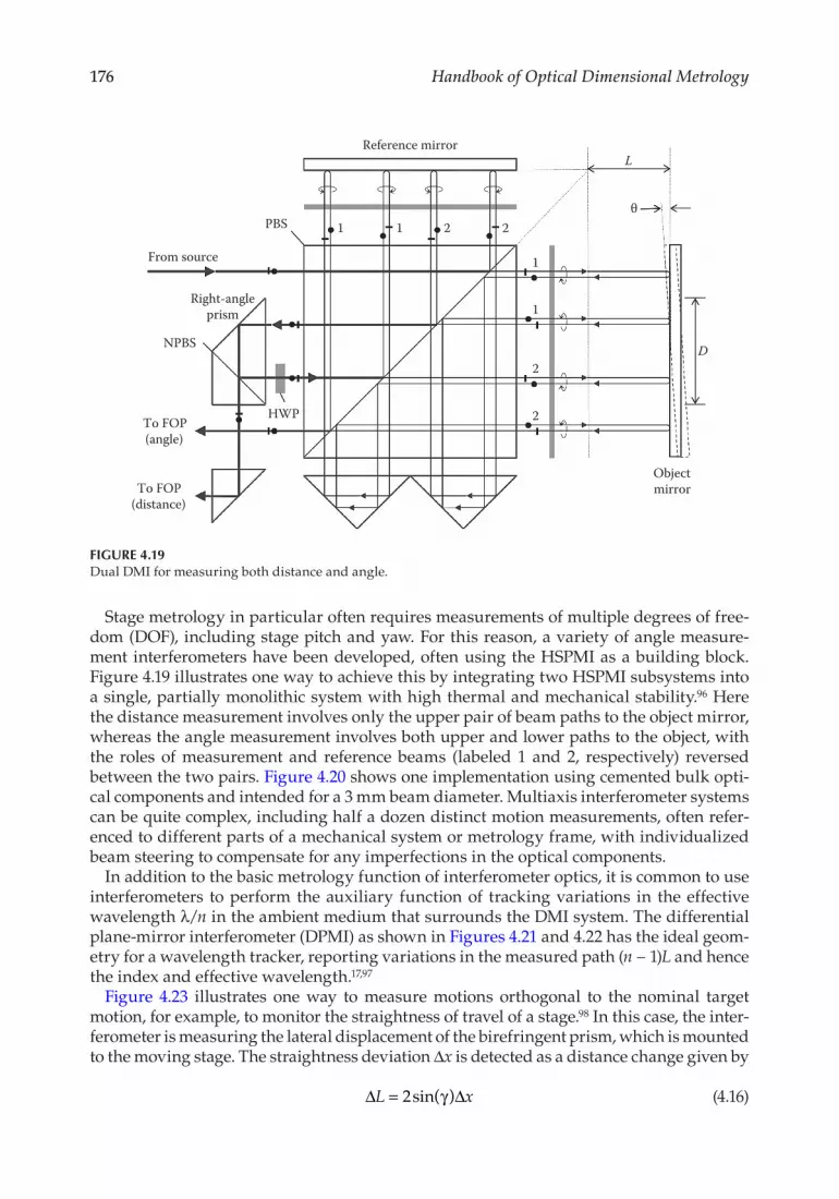
Stage metrology in particular often requires measurements of multiple degrees of free-dom (DOF), including stage pitch and yaw. For this reason, a variety of angle measure-ment interferometers have been developed, often using the HSPMI as a building block. Figure 4.19 illustrates one way to achieve this by integrating two HSPMI subsystems into a single, partially monolithic system with high thermal and mechanical stability.96 Here the distance measurement involves only the upper pair of beam paths to the object mirror, whereas the angle measurement involves both upper and lower paths to the object, with the roles of measurement and reference beams (labeled 1 and 2, respectively) reversed between the two pairs. Figure 4.20 shows one implementation using cemented bulk opti-cal components and intended for a 3 mm beam diameter. Multiaxis interferometer systems can be quite complex, including half a dozen distinct motion measurements, often refer-enced to different parts of a mechanical system or metrology frame, with individualized beam steering to compensate for any imperfections in the optical components.
In addition to the basic metrology function of interferometer optics, it is common to use interferometers to perform the auxiliary function of tracking variations in the effective wavelength λ/n in the ambient medium that surrounds the DMI system. The differential plane-mirror interferometer (DPMI) as shown in Figures 4.21 and 4.22 has the ideal geom-etry for a wavelength tracker, reporting variations in the measured path (n − 1)L and hence the index and effective wavelength.17,97
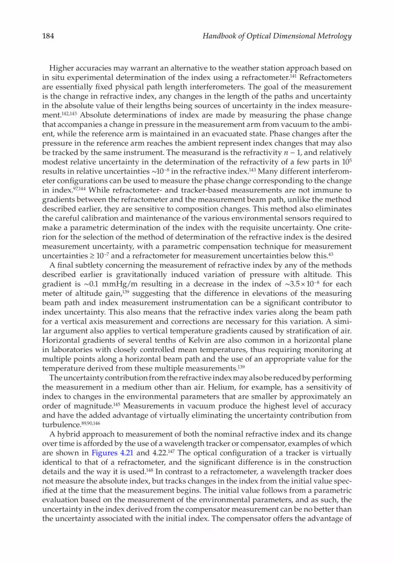
Figure 4.23 illustrates one way to measure motions orthogonal to the nominal target motion, for example, to monitor the straightness of travel of a stage.98 In this case, the inter-ferometer is measuring the lateral displacement of the birefringent prism, which is mounted to the moving stage. The straightness deviation Δx is detected as a distance change given by
∆ ∆L x= 2sin( )γ (4.16)
From source
Right-angleprism
NPBS
To FOP(angle)
To FOP(distance)
HWP
Objectmirror
PBS 1 1
1
1
2 2θ
L
D2
2
Reference mirror
FIGURE 4.19Dual DMI for measuring both distance and angle.

177Displacement Measuring Interferometry
where γ is the angle between the two parts of the dihedral mirror. To first order, this design is insensitive to the tip and tilt of the birefringent prism. In an alternative configuration using the same components, the stage carries the dihedral mirror and the birefringent prism is fixed. This measurement also follows Equation 4.16 but requires the measurement and compensation of the angular motion of the dihedral mirror in the plane of Figure 4.23. With more advanced geometries and considerable care, straightness of travel can be moni-tored and corrected to within a few nanometer over several hundred millimeter of travel.99
In addition to various configurations to measure different types of motion, interferom-eter designs vary according to strategies for reducing error sources. These include spe-cialized components such as polarization-preserving retroreflectors,100 split wave plates to reduce ghost reflections,101 single-pass plane-mirror configurations using dynamically
FIGURE 4.20Compact distance and angle interferometer as in Figure 4.19. The baseplate measures 54 mm. (Photo courtesy of Zygo Corporation, Middlefield, CT.)
To FOP
Polarization splittingshear plate
HWP to rotatepolarization 90°
QWP
PBSWindow
Vaccum cell(reference)
Mirror
L
FIGURE 4.21DPMI configured as a wavelength tracker, using a vacuum cell to detect changes in the ambient index of refraction.
178 Handbook of Optical Dimensional Metrology
steerable components,102 and roof mirror assemblies in place of plane mirrors for stage metrology.103 Figure 4.24, for example, shows a design that reduces errors related to beam mixing using birefringent prisms to encode and decode the measurement and reference beams according to a small difference in propagation angle.104,105 Figure 4.25 illustrates a method of eliminating most sources of cyclic error related to polarization leakage by main-taining the measurement and reference beams fully separated spatially.106–110
4.6 Error Sources and Uncertainty in DMI
Displacement interferometry is capable of producing high-accuracy measurements and is often the ultimate reference standard in many applications. Nonetheless, measurements of displacement using interferometry are like any other measurements in that they have
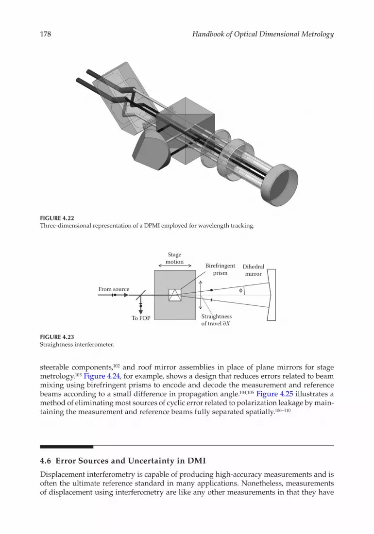
FIGURE 4.22Three-dimensional representation of a DPMI employed for wavelength tracking.
From source
To FOP
Stagemotion Birefringent
prismDihedralmirror
Straightnessof travel ∂X
FIGURE 4.23Straightness interferometer.

179Displacement Measuring Interferometry
sources of error and the required measurement uncertainty determines the suitability of DMI for a given application.111 Any uncertainty estimation requires the identification of the various contributing sources as a first step followed by appropriate combination of these.
This section discusses the most significant contributing sources of uncertainty in the context of a typical measurement—a simple linear interferometer configuration with a corner-cube target for the measurement of the displacement of a linear stage. Figure 4.26 indicates two distinct displacements: the measurand D, which is a displacement of the POI on the stage, and the measured displacement Dm. In general, because of the various sources of error, the measurand D and the measured displacement Dm are not the same.
The relationship between the various quantities defined earlier is
D D Dm i
i= + ∑ δ (4.17)
From source
Birefringentprism
Referenceretroreflector
Objectretroreflector
PBS(imperfect)
To FOP
FIGURE 4.24Interferometer using birefringent elements to overcome imperfect polarization separation of the reference and measurement beams at the beam splitter. (From de Groot, P.J. et al., US 6, 778, 280, 2004.)
Reference channel
AOM
AOM
f1
f2
Movingroof mirror
Fixedroof mirror
Measurement channel
FIGURE 4.25Unpolarized, separated beam interferometer using AOMs. (From Tanaka, M. et al., IEEE Trans. Instrum. Meas., 38, 552, 1989.)

180 Handbook of Optical Dimensional Metrology
where δDi represents displacements not directly attributable to the measurand and will henceforth be referred to as spurious displacements, each of which contributes to the uncer-tainty in the measurand u(D) through associated uncertainties ui(D). In the absence of any spurious displacements, D would equal the measured displacement Dm, and u(D) would equal the uncertainty in the measured displacement u(Dm). Expressing Dm in Equation 4.17 in terms of the phase change Δϕ that corresponds to the measured displacement Dm, we have112
D
NDi
i= ′
+ ∑λ
βφπ
δcos( )
∆2
(4.18)
whereN is an integer factor that depends on the number of passes (round-trips) of the measure-
ment beam to the target and backλ′ (the effective wavelength) is the ratio of the vacuum wavelength λ and the index of
refraction ncos(β) results from the angular misalignment β between the direction of motion of the
stage and the beam
For the particular configuration of Figure 4.26, the number of round-trip passes N = 2. Equation 4.18 serves as a mathematical model of the measurement and forms the basis of the discussion of uncertainty sources in the following sections. An overall uncertainty for the measurement combines the various contributions according to the procedures of the Guide to the Expression of Uncertainty in Measurement (GUM).113
4.6.1 Uncertainty Sources
The majority of the contributors fall into two broad categories:Category 1—uncertainty in the value of a parameter. Uncertainty contributors in this cat-egory are relatively few in number and correspond to most of the quantities in the first term of Equation 4.18. These contributors generate uncertainties that are proportional to the measurand, that is, their magnitude scales with the displacement D.
POI
Stage
Base
Dm
D
FIGURE 4.26An arrangement to measure the displacement of a linear stage.

181Displacement Measuring Interferometry
Category 2—uncertainty from sources that affect the measurand but in fact are not directly attributable to it, that is, from spurious displacements. These contributors are represented by Δϕ and the second term of Equation 4.18, and unlike the contributors in Category 1, the magnitude of these contributions is not dependent on D.Table 4.2 is a nonexhaustive list of common contributors in each of the earlier categories. Many of the contributors common to other measurement techniques (e.g., cosine error and Abbe error) are included here clarify their interpretation in the context of interferometric displacement measurement. Some uncertainty sources that are common to any measure-ment technique, for example, thermal changes in the metrology frame, are not discussed here but would contribute as they would in any measurement.
4.6.2 Vacuum Wavelength
The vacuum wavelength λ establishes the linkage between the unit of length and the change in phase, and any associated uncertainty u(λ) contributes directly in the calculated displacement. The uncertainty in the measurand uλ(D) depends on the relative uncertainty in the wavelength u(λ)/λ and is proportional to the measurand as given by114,115
u D u Dλ
λλ
( ) ( )= (4.19)
Uncertainty in the vacuum wavelength λ has multiple contributors: the uncertainty in the determination of the absolute value of the wavelength and a contribution arising from short- and long-term drift.116,117 Displacement interferometers typically use stabilized He-Ne lasers emitting at 633 nm as the light source, and the uncertainty in the wavelength and the associated stability depends on the method of stabilization as summarized in Table 4.1. For applications demanding a lower uncertainty in the vacuum wavelength, a reference laser such as an iodine-stabilized laser may be included within the system and used to monitor the wavelength of the metrology laser used for interferometry.89,90
In the case of two-frequency laser sources intended for use in heterodyne systems, a rather subtle error can result from the slightly different nominal vacuum wavelength for the two beams of slightly different frequencies (and different polarizations). The difference depends on the frequency difference (or split frequency). In such systems, it is important
TABLE 4.2
Typical Sources of Uncertainty in Displacement Interferometry
Category 1 Category 2
Uncertainty in vacuum wavelengthUncertainty in refractive index arising from either absence of correction or uncertainty in inputs to correction
Cosine error
Uncertainty in the measurement of phase change
Effect of deadpathCyclic errorsOptics thermal driftAbbe errorsTarget errorsBeam shearData age uncertaintyTurbulenceTarget mounting effects

182 Handbook of Optical Dimensional Metrology
to keep track of the wavelength of the beam in the measurement arm and to scale the mea-sured phase by the appropriate wavelength. Failure to do so results in a systematic error in the measured displacement, which can be significant depending on the application.
4.6.3 Refractive Index
Both the refractive index n and the vacuum wavelength λ relate directly to the traceability of displacement measurement.118 Since λ′ = λ/n scales the measured phase change into units of length, any uncertainties associated with the index u(n) affect λ′ and the measurand directly, that is, the uncertainty in the measurand due to index uncertainty un(D) is a direct function of the relative uncertainty in the index and is also proportional to the displacement:115
u D u n
nDn( ) ( )= (4.20)
DMI measurements are typically in air, and the refractive index of air nair is dependent on several environmental variables such as the pressure P, the temperature T, the moisture content or humidity H, and the exact composition. This can lead to significant variations in nair depending on the prevailing environmental conditions and/or deviations from the assumed composition at the time of the measurement.
A nominal value for nair follows from the so-called weather station approach119 or from a direct measurement using refractometers of various kinds.97,120 This first method is more pragmatic and relies on the measurement of P, T, and H, using instrumentation to provide the required inputs for index calculation. Fortunately, the refractive index of air is a well-characterized function of P, T, and H in the form of the empirical equations developed by several investigators.121–125 An expression commonly used today for dimensional metrology applications under laboratory conditions, that is, at temperatures near 20°C, is a modified form126,127 of the expression introduced by Edlén.122 The modified Edlén equation, some-times referred to as the NPL revision, was developed to account for discrepancies between the experimentally measured and calculated values and to also incorporate changes to the International Temperature Scale (ITS) instituted after the publication of Edlén’s original equa-tion. The modified equation agrees with experimental values128 to within 3 × 10⁻⁸(3σ) and to a few parts in 108 in more recent investigations.129,130 The complete (and somewhat cumber-some) expression, which is actually a set of three linked equations, appears in the paper by Birch and Downs.126,127 More recently developed equations by Ciddor apply over a larger wavelength range and more extreme environmental conditions to the stated uncertainty.131–133
While the full expression calculates the nominal value of the index corresponding to a set of environmental conditions, the uncertainty associated with this calculated value follows from the partial derivatives with respect to each of the environmental parameters for a vacuum wavelength of ∼633 nm. These derivatives are then evaluated at standard conditions (P = 101325 Pa, T = 293.15 K, and H = 50%) to give sensitivities KT, KP, and KH of the index of air to changes in temperature, pressure, and humidity,134 numerical values for which are provided in Equation 4.21:
K
K
T
P
= − × − ×
= + × + ×
− −
− −
0 927 10 1 10
2 682 10 1 10 3
6 6
9 6
. / ~ /
. / ~ /
K or K
Pa or mmm Hg
RH or %RHKH = − × − ×− −0 01 10 1 10 1006 6. /% ~ /
(4.21)

183Displacement Measuring Interferometry
The equation also gives (in round numbers) the required changes in key environmental parameters to produce a 1 × 10⁻⁶ change in the index in more commonly used units. The refractive index is most sensitive to changes in temperature and pressure with relatively large changes in humidity being required to cause a comparable change in the index. Note that the coefficients are signed, and while this usually is not of consequence in the deter-mination of the uncertainty, it is critical in establishing the sign of the error. The associated uncertainty u(nair) is a function of the uncertainties in the temperature u(T), pressure u(P), and humidity u(H) and is given by115,134
u n K u T K u P K u Hair T P H( ) ( ) ( ) ( )= + +2 2 2 2 2 2 (4.22)
There is also an “intrinsic” uncertainty associated with this empirical expression that derives from the uncertainty in the data used to derive them.121,135 In other words, even if the inputs to the equation are known exactly, there is an uncertainty in the calculated index that results from the uncertainty in the coefficients of the modified Edlén equation. The developers of the equation estimate this uncertainty contribution to be 3 × 10⁻⁸(3σ), or a standard uncertainty of 1 × 10⁻⁸ or 10 parts per billion (ppb), corresponding to 10 nm in a displacement over 1 m.126,127 This intrinsic uncertainty should be included in determina-tions of u(nair).136 In almost all practical applications, contributions from the uncertainties associated with the determination of the input parameters dwarf this contribution.
The weather station method depends on fixed assumptions regarding the composition, potentially leading to an important uncertainty in the calculated index. The modified Edlén assumes a CO2 concentration of 450 × 10−6.126 The CO2 concentration can vary—a prime example is a higher than assumed concentrations of CO2 caused by human respi-ration.137 Fortunately, changes in the index of ∼2 × 10⁻⁸ require a change in CO2 concen-tration of 150 × 10−6 and only become significant in the most demanding applications.138 A more significant contribution is due to changes in composition due to the presence of hydrocarbons, for example, acetone, which causes an index change of 10−7 for a contami-nation level of 130 × 10−6.59 Solvent vapors are present in many metrology environments, for example, the metrology of optics, where solvents such as acetone, alcohol, and various other volatile solvents are often used for cleaning, resulting in marked deviations from the assumed composition. The composition of the air is not typically monitored in such environments, although in general the presence of a detectable odor is a good indication of the presence of a volatile hydrocarbon at levels that are significant for the highest accu-racy measurments.59 One way this contribution may be incorporated into Equation 4.22 is via an additional term that captures the uncertainty in the concentration of the particular hydrocarbon and the appropriate sensitivity.
For high-accuracy determinations of the index, great care is required in making mea-surements of temperature, pressure, and humidity, as described in the classic paper by Estler.139 The measurements of the environmental parameters now also become part of the traceability chain.118 Recent refractometer comparisons have shown that it is possible with careful measurements to reduce the contribution from uncertainties in the input parameters to the point where the uncertainties in the parameters of the modified Edlén equation are comparable or even dominate.120,130 This however requires extremely careful measurements of the input parameters, something that is typically not easily achieved in nonlaboratory measurements. Factors such as the location of the sensors, gradients in temperature and pressure, thermal inertia, and self-heating of sensors also complicate the measurement of environmental parameters.140
184 Handbook of Optical Dimensional Metrology
Higher accuracies may warrant an alternative to the weather station approach based on in situ experimental determination of the index using a refractometer.141 Refractometers are essentially fixed physical path length interferometers. The goal of the measurement is the change in refractive index, any changes in the length of the paths and uncertainty in the absolute value of their lengths being sources of uncertainty in the index measure-ment.142,143 Absolute determinations of index are made by measuring the phase change that accompanies a change in pressure in the measurement arm from vacuum to the ambi-ent, while the reference arm is maintained in an evacuated state. Phase changes after the pressure in the reference arm reaches the ambient represent index changes that may also be tracked by the same instrument. The measurand is the refractivity n − 1, and relatively modest relative uncertainty in the determination of the refractivity of a few parts in 105 results in relative uncertainties ∼10−8 in the refractive index.143 Many different interferom-eter configurations can be used to measure the phase change corresponding to the change in index.97,144 While refractometer- and tracker-based measurements are not immune to gradients between the refractometer and the measurement beam path, unlike the method described earlier, they are sensitive to composition changes. This method also eliminates the careful calibration and maintenance of the various environmental sensors required to make a parametric determination of the index with the requisite uncertainty. One crite-rion for the selection of the method of determination of the refractive index is the desired measurement uncertainty, with a parametric compensation technique for measurement uncertainties ≥ 10−7 and a refractometer for measurement uncertainties below this.43
A final subtlety concerning the measurement of refractive index by any of the methods described earlier is gravitationally induced variation of pressure with altitude. This gradient is ∼0.1 mmHg/m resulting in a decrease in the index of ∼3.5 × 10⁻⁸ for each meter of altitude gain,139 suggesting that the difference in elevations of the measuring beam path and index measurement instrumentation can be a significant contributor to index uncertainty. This also means that the refractive index varies along the beam path for a vertical axis measurement and corrections are necessary for this variation. A simi-lar argument also applies to vertical temperature gradients caused by stratification of air. Horizontal gradients of several tenths of Kelvin are also common in a horizontal plane in laboratories with closely controlled mean temperatures, thus requiring monitoring at multiple points along a horizontal beam path and the use of an appropriate value for the temperature derived from these multiple measurements.139
The uncertainty contribution from the refractive index may also be reduced by performing the measurement in a medium other than air. Helium, for example, has a sensitivity of index to changes in the environmental parameters that are smaller by approximately an order of magnitude.145 Measurements in vacuum produce the highest level of accuracy and have the added advantage of virtually eliminating the uncertainty contribution from turbulence.89,90,146
A hybrid approach to measurement of both the nominal refractive index and its change over time is afforded by the use of a wavelength tracker or compensator, examples of which are shown in Figures 4.21 and 4.22.147 The optical configuration of a tracker is virtually identical to that of a refractometer, and the significant difference is in the construction details and the way it is used.148 In contrast to a refractometer, a wavelength tracker does not measure the absolute index, but tracks changes in the index from the initial value spec-ified at the time that the measurement begins. The initial value follows from a parametric evaluation based on the measurement of the environmental parameters, and as such, the uncertainty in the index derived from the compensator measurement can be no better than the uncertainty associated with the initial index. The compensator offers the advantage of

185Displacement Measuring Interferometry
higher bandwidth in that it responds virtually instantaneously to changes in index when compared to the time delay inherent in the measurement of the environmental parameters.
4.6.4 Air Turbulence
Air turbulence arises from the high airflow rates that are required in high-precision machinery in order to control the temperature, ensure cleanliness, etc., and their interac-tions with the often cramped confines of such equipment. Turbulence causes time-depen-dent variations in the index of refraction in the beam paths through localized pressure and temperature fluctuations, and the resulting optical path length changes manifest themselves as relatively high-frequency random fluctuations in the measured displace-ment.149 In high-accuracy applications such as microlithography, turbulence can often be the leading source of uncertainty.150 Turbulence also affects the measurement through direct interactions of the airflow with components within the metrology loop such as mir-rors and mounts, resulting in vibrations that contribute to the observed optical path length fluctuations.
While much data are available on the effects of atmospheric turbulence on the propaga-tion of radiation, data on turbulence as they relate to typical interferometric applications (particularly lithographic applications) are scarce, and much of the discussion here draws from Bobroff’s now classic paper on the subject.149 The magnitude of the contribution from turbulence scales with the length of path of the beams and a first level mitigation strat-egy is to minimize the lengths of air path, a measure that also minimizes the contribu-tions due to deadpath (see Section 4.6.8). The RMS magnitude of the fluctuations can vary from subnano-meter levels for enclosed beam paths to approximately 2.5 nm for flow rates of 100 linear feet per minute (LFM) perpendicular to the beam direction over a 150 mm length of exposed beam path.149
Another consequence of turbulence is its effect on correlation in the OPL fluctuations observed in two parallel beams. This has important implications for interferometer con-figurations of the column-reference type, wherein the measurement and reference beams monitor targets attached to two metrologically significant parts of the machine or struc-ture between which a differential measurement is desired, for example, the projection lens and the wafer in a microlithographic tool. In this configuration, the two beam paths are typically parallel and almost the same length (except for the stage travel in the mea-surement arm). In the absence of turbulence, index changes are correlated in the common portions of the two arms, thereby rejecting deadpath contributions to a high degree. In the presence of turbulence, this correlation decreases and cancelation is not as complete at high frequencies. A similar situation prevails in situations where two spatially separated interferometers working against a common target mirror measure angular motion of the mirror. In this configuration, the measurement arms of the two interferometers are paral-lel, and the lack of correlation is a source of uncertainty in the angle measurement.
Time averaging can minimize the effects of turbulence. The averaging period depends on the time scale of the phase fluctuations, and in general this gain comes at the expense of data rate, making it impractical for applications with high servo loop frequencies. Turbulence can also lead to mechanical noise in high-bandwidth systems as the controller attempts to compensate for the high-frequency changes in the measured displacement.
Another approach to minimizing the effects of turbulence is the careful design of flow paths and in general reducing the exposed paths to a minimum. Shielding the paths is effective, although this is not always practical in the measurement beam path. Turbulence can be eliminated by operating the interferometers in evacuated pathways89,151 or by
186 Handbook of Optical Dimensional Metrology
enclosing the entire device in a vacuum as is often done in extreme ultraviolet lithography (EUVL) machines152 and electron-beam lithography machines.153 Another, more specula-tive approach is dispersion interferometry, described in Section 4.8.3.
4.6.5 Cosine Error
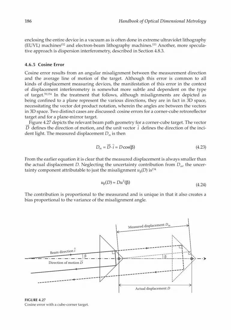
Cosine error results from an angular misalignment between the measurement direction and the average line of motion of the target. Although this error is common to all kinds of displacement measuring devices, the manifestation of this error in the context of displacement interferometry is somewhat more subtle and dependent on the type of target.59,154 In the treatment that follows, although misalignments are depicted as being confined to a plane represent the various directions, they are in fact in 3D space, necessitating the vector dot product notation, wherein the angles are between the vectors in 3D space. Two distinct cases are discussed: cosine errors for a corner-cube retroreflector target and for a plane-mirror target.
Figure 4.27 depicts the relevant beam path geometry for a corner-cube target. The vector D
defines the direction of motion, and the unit vector i defines the direction of the inci-dent light. The measured displacement Dm is then
D D i Dm = ⋅ = cos( )β (4.23)
From the earlier equation it is clear that the measured displacement is always smaller than the actual displacement D. Neglecting the uncertainty contribution from Dm, the uncer-tainty component attributable to just the misalignment uβ(D) is134
u D Duβ β( ) ( )≈ 2 (4.24)
The contribution is proportional to the measurand and is unique in that it also creates a bias proportional to the variance of the misalignment angle.
Actual displacement D
Measured displacement Dm
Beam direction i
Direction of motion D
β β
FIGURE 4.27Cosine error with a cube-corner target.
187Displacement Measuring Interferometry
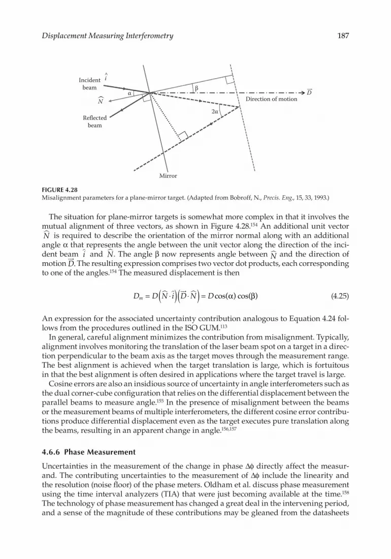
The situation for plane-mirror targets is somewhat more complex in that it involves the mutual alignment of three vectors, as shown in Figure 4.28.154 An additional unit vector N is required to describe the orientation of the mirror normal along with an additional angle α that represents the angle between the unit vector along the direction of the inci-dent beam i and N. The angle β now represents angle between N and the direction of motion D
. The resulting expression comprises two vector dot products, each corresponding
to one of the angles.154 The measured displacement is then
D D N i D N Dm = ⋅( ) ⋅( ) = cos( ) cos( )α β (4.25)
An expression for the associated uncertainty contribution analogous to Equation 4.24 fol-lows from the procedures outlined in the ISO GUM.113
In general, careful alignment minimizes the contribution from misalignment. Typically, alignment involves monitoring the translation of the laser beam spot on a target in a direc-tion perpendicular to the beam axis as the target moves through the measurement range. The best alignment is achieved when the target translation is large, which is fortuitous in that the best alignment is often desired in applications where the target travel is large.
Cosine errors are also an insidious source of uncertainty in angle interferometers such as the dual corner-cube configuration that relies on the differential displacement between the parallel beams to measure angle.155 In the presence of misalignment between the beams or the measurement beams of multiple interferometers, the different cosine error contribu-tions produce differential displacement even as the target executes pure translation along the beams, resulting in an apparent change in angle.156,157
4.6.6 Phase Measurement
Uncertainties in the measurement of the change in phase Δϕ directly affect the measur-and. The contributing uncertainties to the measurement of Δϕ include the linearity and the resolution (noise floor) of the phase meters. Oldham et al. discuss phase measurement using the time interval analyzers (TIA) that were just becoming available at the time.158 The technology of phase measurement has changed a great deal in the intervening period, and a sense of the magnitude of these contributions may be gleaned from the datasheets
Incidentbeam
Reflectedbeam
Mirror
Direction of motionD
2α
α
^
N
iβ
FIGURE 4.28Misalignment parameters for a plane-mirror target. (Adapted from Bobroff, N., Precis. Eng., 15, 33, 1993.)

188 Handbook of Optical Dimensional Metrology
of commercially available phase measurement electronics159 and manufacturer’s published guides to uncertainty.111 Accuracy figures are quoted for various measurement velocities of the target, with the accuracy number when the target is stationary representing the “static accuracy” or alternately the noise floor of the electronics. The accuracy numbers at different target velocities are a measure of the “dynamic accuracy” and in general tend to be larger than the noise floor of the instrument as they also include contributions from nonlinearities of the phase meter. The noise floor of the instrument is a strong function of the signal levels, and manufacturer’s specifications assume a certain signal level, both in terms of the total amount of light at the detector as well as the depth of modulation of the AC signal.18 Heterodyne interferometers have a distinct advantage over homodyne interferometers in the achievable noise floor for a given optical power. The shift in the operating point of the heterodyne interferometer away from DC and the large 1/f noise background makes it possible to achieve an extremely low noise floor in the presence of very low optical powers. This in turn makes it possible to illuminate a dozen or more mea-surement channels from a single laser source without sacrificing the noise performance.
In some applications where the length standard is established independently, for exam-ple, by the spacing between fiducials on a physical artifact, the uncertainty in the value of scaling factor resulting from uncertainties in the index, vacuum wavelength, alignment, etc., is much less important. This scenario is encountered in applications such as lithography where the measurement between two or more fiducials on the wafer sets the length scale and the interferometer system then simply serves to access locations relative to the coordinate system so established. The stability of the various scaling terms becomes far more important to guarantee the stability of this calibration for the duration of the measurement.
4.6.7 Cyclic Errors
Periodic or cyclic errors are characteristic of all systems that rely on phase estimation. Figure 4.29 shows small signal fluctuations and the typical periodic or cyclic error related to known component and alignment imperfections. Although most generally a cyclic error may have any cause that correlates to interference phase, in DMI, the most common ori-gins relate to insufficient isolation of the measurement and reference beams as they travel through the optical system or the admixture of unwanted reflected or scattered beams.
The estimation of the uncertainty contribution of cyclic errors is somewhat trick-ier because they are sinusoidal. Monte Carlo simulations graphically demonstrate the
11.8
12.0
12.2
12.4
12.6
12.8 1.0
0.5
–0.5
–1.0
0
Displacement (nm)
Signal (%) Displacement error (nm)
Displacement (nm)0 100 200 300 400 500 0 100 200 300 400 500
(a) (b)
FIGURE 4.29Simulations of signal fluctuation (a) and cyclic displacement measurement error (b) in a plane-mirror DMI system.

189Displacement Measuring Interferometry
U-shaped distributions that result from these errors.160 The standard uncertainty for these contributors may be calculated by assuming an underlying sinusoidal probability distri-bution function and scaling the amplitudes appropriately.115
Evaluating cyclic error sources and magnitudes begins with a model of the optical sys-tem, starting with a functional block diagram such as is shown in Figure 4.30. A significant amount of attention has been devoted to quantifying and mitigating errors arising from polarization mixing, ghost reflections, and other sources of spurious signals that result in periodic nonlinearities.161,162 The importance of polarization separation implies that Jones calculus notation is a suitable approach to representing each of the blocks or functional elements mathematically for subsequent analysis.163,164
In one such representation of the DMI system, the heterodyne optical signal is given by165
I = ⋅ ⋅ ⋅ ⋅Mix Int Src Frq Las 2 (4.26)
where the three-letter variables are mnemonics correspond to the functional blocks in Figure 4.30, in reverse order. A vector Las represents the laser source, emitting equally in the s and p polarization states, represented by the two elements of the vector:
Las =
12
11
(4.27)
The next functional matrix Frq corresponds to the device that provides a frequency shift between the two polarizations:
Frq( )t
ee
i f t
i f t=
+
−
π
π
∆
∆
00
(4.28)
The product
Frq⋅ =
+
−Las 1
2e
e
i f t
i f t
π
π
∆
∆ (4.29)
Laser Frequencyshifter
Sourceimperfections
Interferometeroptics
Mixer and fibercoupler
Heterodyneoptical signalObject mirror
FIGURE 4.30Functional block diagram of a heterodyne DMI measurement axis.

190 Handbook of Optical Dimensional Metrology
represents a heterodyne light source with a two-frequency emission encoded by polariza-tion, with a frequency difference Δf.
Continuing with Equation 4.26, the Jones matrix Src for source imperfections comprises potential contributions such as alignment errors, polarization ellipticity, and noise. An example contributor is orthogonality of the polarization states carrying the two source frequencies. The corresponding Jones matrix is
ort( )cos sinsin cos
,δχδχ δχ
δχ δχ=
( ) − ( )− ( ) ( )
2 22 2
(4.30)
where typically δχ is on the order of 10 mrad. The Src matrix is the product of ort and all of the other Jones matrix representations of source errors.165
The Jones matrix Int corresponds to the interferometer optics and depends of course on the specific optical geometry. Taking as an example a Michelson interferometer as in Figure 4.2 and assuming perfect alignment,
Int Ref Mes( ) ( ),L L= + (4.31)
where
Mes pbs U rtr U pbsT T( ) ( ) ( )L L L= ⋅ ⋅ ⋅ ⋅ (4.32)
and
Ref pbs U rtr U pbsR R= ⋅ ⋅ ⋅ ⋅( ) ( )L L (4.33)
Table 4.3 lists the component matrices. The final matrix to complete the model is the polar-izer to combine the reference and measurement beams:
Mix anl( ) ( )α αmix mix= (4.34)
There are several additional error sources not discussed here, including surface reflections and errors that vary with stage angle. All of these errors are incorporated into more exten-sive Jones matrix models. Computer simulation is straightforward using modeling of this type, leading to Figure 4.29.
Of several possible techniques for quantifying cyclic errors experimentally, the most effective is by Fourier or spectral analysis of the interference signal while the object mir-ror is in motion, resulting in a Doppler shift that separates the errors by frequency.166–168 Figure 4.31 illustrates such an analysis for a DPMI (as in Figure 4.21), showing the desired heterodyne peak labeled 1 in the figure and a number of secondary peaks, all correspond-ing to unwanted periodic errors.169 The displacement-equivalent amplitudes of peaks 2, 3, 4, 5, and 6 in this example are 4, 2, 1.2, 0.6, and 0.1 nm, respectively. Each of these peaks is associated with specific cyclic errors. For example, peaks 4 and 5 are leakage at the PBS (interferometer errors) and polarization mixing in the light source (source imperfections). In many cases, an adjustment of the interferometer optics, for example, by tilting compo-nents or adjusting wave plate orientation, can reduce several of these errors interactively while observing the spectral analysis in real time.170

191Displacement Measuring Interferometry
4.6.8 Deadpath
Deadpath is the difference in optical path length of the reference and measurement beams when the interferometer electronics are zeroed.171 This is not necessarily the position of closest approach of the target to the interferometer as emphasized by Figure 4.32.
The imbalance between the two arms results in a sensitivity to both changes in index Δn and source wavelength Δλ, the consequence of which is to shift the point in space at which
010
102
103
104
105
106
0.2
5
3
1
2
4
6
0.4 0.6Frequency (Nyquist)
Am
plitu
de (a
rb. u
nits
)
0.8 1.0
FIGURE 4.31Spectral analysis of the heterodyne interference signal in a DPMI. (From Hill, H.A., Tilted interferometer, U.S. Patent 6,806,962, 2004.)
TABLE 4.3
Interferometer Component Jones Matrices
Matrix Name Matrix Form Typical Values
Beam propagation U Ix i x( ) = ⋅
exp 2πλ λ = 632.8 nm
Antireflection coatings arc I= ⋅ TA TA = 99.5%
Polarizer pol( , )a ba
b=
00
—
Cube beam splitter reflection pbsR = arc · pol(Rcs, Rcp) · arc Rcs = 99.9%Rcp = 0.1%
Cube beam splitter transmission pbsT = arc · pol(Tcs, Tcp) · arc Tcs = 0.1%Tcp = 99.9%
Beam propagation U I( ) expx i x= ⋅
2πλ
λ = 632.8 nm
Polarization rotation rot( )cos( ) sin( )sin( ) cos( )
ϑϑ ϑϑ ϑ
=−
—
Corner-cube retroreflector rtr arc rot arc= ⋅ ⋅Rrtr ( )ζ Rrtr = 80%ζ = 85 mrad
Mixing polarizer (dichroic analyzer) anl arc rot
pol rot
( ) ( )
( , ) ( )
δα δα
δα
mix mix
mix mixT
= ⋅ ° +
⋅ ⋅ − ° − ⋅
45
0 45 aarc
δαmix = 10 mrad
Tmix = 80%

192 Handbook of Optical Dimensional Metrology
the zero location of the interferometer was established (hence the alternate use of the term “zero-shift” error). An equal index change results in an unequal change in the optical path lengths in the two arms, resulting in a spurious displacement.166 Variation of the source wave-length generates a similar effect. Even though changes in wavelength and index are typically compensated, these corrections usually apply only to the measured displacement, because a displacement interferometer is blind to any initial imbalance between the two arms.
The deadpath error δDDP for a length difference L0 = Li − LR between the initial position of the target and the reference arm is172
δD L n
nDP n, ∆∆=
− 0 (4.35)
for changes Δn = nf − ni in refractive index and
δ λ
λλD LDP,∆∆=
0 (4.36)
for changes Δλ = λf − λi wavelength. Here the subscripts i and f stand for the value at the beginning and end of the measurement, respectively. This definition of the deadpath assumes that the computation of the displacement uses the final values of wavelength and index in Equation 4.18, a different expression being applicable when a value other than the final value is used.173 The deadpath contribution is proportional to the length of deadpath, although it is independent of the magnitude of the measurand. The corresponding uncer-tainty contributions from the deadpath, neglecting the term due to the uncertainty in the deadpath length itself, are172
u D L u n
nDP n, ( ) ( )∆
∆= 0 (4.37)
Li
Dm
Dm
Li
Interferometer“zero”
Interferometer“zero”
LR
LR
FIGURE 4.32Initial position determines deadpath Li. Lower figure has longer deadpath.

193Displacement Measuring Interferometry
and
u D L uDP, ( ) ( )
∆∆
λλ
λ= 0 (4.38)
where u(Δn) and u(Δλ) are the standard deviation in the index and source wavelength variation over the period of the measurement.
There are a number of different ways to address the deadpath contribution. A simple software solution is to preset the phase meter with a value corresponding to L0 such that the interferometer displays this value at the “zero” position. This makes the interferometer system “aware” of the deadpath length and thus subject to the corrections for index and wavelength. The correction afforded by this technique has a residual uncertainty caused by the uncertainty in the determination of the deadpath length that must be included into the overall measurement uncertainty. Another solution relies on reducing L0 to the minimum allowed by the constraints of the interferometer lay-out. This typically involves moving the interferometer as close to the zero position of the target as possible, by a combination of physical arrangement of the optics and by zeroing out the interferometer when the target is at its point of closest approach to the interferometer.171 Another option may be to increase the length of the reference arm to match the distance to the zero position in the measurement arm, at the expense of the stability of the system. This of course assumes that both arms experience the same changes in index. Another zero-shift estimation applicable to certain applications such as scale measurement requires retaking a “zero” reading after a measurement cycle, any discrepancy being a representation of drift including the zero shift over the measurement cycle.43
4.6.9 Abbe Error
Abbe in 1890 first enunciated the Abbe principle, sometimes referred to as the comparator principle.174 Revised by Bryan,175 the Abbe principle articulates the notion that the line of measurement should coincide with the line along which the displacement measurement is desired in order to reject the contributions that arise from parasitic angular error motions of the object being monitored. Figure 4.33 is a schematic representation of a measurement scenario wherein the measurement axis of the linear interferometer is off-set from the mounting surface of the stage where the POI in the definition of the measur-and D is located. The nodal point of the retroreflector target establishes the location of the measurement axis, and the beam direction establishes the orientation of this axis,59 resulting in an Abbe offset Ω between the line of measurement and the POI. The figure depicts the effect of a parasitic pitch or angular motion of the stage in the plane of the fig-ure. For the sake of clarity, only the retroreflector and its mount are shown rotated by an angle θ, rather than showing the entire stage rotated through this angle. In the presence of an angular error motion θ and an offset Ω, the Abbe error is δDAbbe. The magnitude of the error is
δ θ
θ θ
DAbbe =
≈
Ω
Ω
tan
(forsmall ) (4.39)

194 Handbook of Optical Dimensional Metrology
Simplifying the expression given by Schmitz134 using the small angle approximation gives the associated uncertainty contribution:
u d u uAbbe2 2 2 2 2( ) ( ) ( )= +θ θΩ Ω (4.40)
The value of the angle θ and u (θ) typically derives from a priori knowledge of the angular error motions of the stage, for example, specification sheet for the stage or measurements, while Ω depends on the target type and the beam alignment technique. There are typi-cally two Abbe offsets (usually in two mutually orthogonal directions) for any POI and two accompanying angular error motions (about the two mutually orthogonal directions identified earlier). In other words, an expression analogous to Equation 4.40 describes a second contribution from the Abbe offset in the orthogonal direction and angular motions about that direction. In the simplest case where the error motions in the two directions are uncorrelated, the contributions that result from the two offsets combine in quadrature. In a more realistic scenario where the motions are not likely to be totally uncorrelated, an additional term that accounts for the correlation must be included.113
The stipulation that the line of measurement passes through the POI requires a way to identify the line of measurement. This in turn means identifying the orientation in space of the line of measurement and a point through which it passes relative to some features in the measurement setup. While this is typically easy to do with many kinds of displace-ment measuring devices, for example, LVDT and encoder scales, the identification of the line of measurement for an interferometer system is more subtle and depends on the type of interferometer and target. Figure 4.34, for example, shows the line of measurement for a two-pass PMI (as in Figure 4.15) and a single-pass retroreflector interferometer. For the PMI, the line of measurement is parallel to the normal N.154 Further, the fact that the phase change reported by the interferometer is the average of the phase change in each of the encounters with the mirror also means that the line of measurement is located midway between the two measurement beams. In contrast, the orientation i of the incident beam sets the orientation of the line of measurement for a retroreflector interferometer parallel to i in Figure 4.34, while the nodal point or optical center of the corner cube establishes the
Stage
Base
POI
θ
Ω
δDAbbe
Dm
D
FIGURE 4.33Abbe offset and the resulting error.

195Displacement Measuring Interferometry
measurement location.59,176 In the case of the PMI, the location of the line of measurement has to be determined in reference to a virtual datum, that is, the location of the two light beams. This implies a certain level of uncertainty in setting the location of the line relative to the POI. Experience suggests that one can usually minimize the Abbe offsets to approxi-mately 0.5 mm for standard beam diameters without special measures. A smaller value is achievable when using a corner cube because the reference point is precisely manufac-tured, although it may be inaccessible in some cases due to the retroreflector mounting. The limit to the accuracy of placement is typically the tolerance stack up and/or fixturing used to locate the corner cube.
Interferometers are particularly well suited to measurement configurations designed to minimize the Abbe offset as they establish a virtual axis of measurement that has no mechanical interference with other parts of the system. A family of coordinate measuring machines (CMM) typifies this approach, wherein the interferometer axes are in line with the probe.177,178 In the relatively rare situations where the POI is not directly accessible or the measurement of multiple DOF is desired, multiple interferometers and appropriately weighted outputs establish a virtual measurement axis.134,179
Additional strategies to mitigate the impact of any residual Abbe offset include driving the angular error motion θ to zero or measuring the angular error motions and applying a correction. In a first scenario, eliminating the angular motion minimizes the contribution, usually through active control, so that the angle θ and the first-order Abbe error are nominally zero.180,181 The uncertainty contribution results from any residual angular motions.
A second approach relies on the measurement of the angular motions.182 While the angle θ may be measured using a secondary measurement device, interferometers have an advan-tage in that there are many interferometer configurations that measure displacement and angle simultaneously, making it convenient to implement the desired correction.183,184 The uncertainty of the correction is now driven by uncertainty in the determination of the angle θ. This type of compensation applies only to rigid body motions, that is, there is the implicit assumption that there are no significant internal bending-type deformations within the monitored body. If these kinds of deformations are anticipated and the desired level of measurement accuracy demands it, a higher level of correction based on the mea-surement of the deformation is required, or the Abbe offset must be eliminated.
Plane mirror
Line ofmeasurement
Cube-cornerretroreflector
l
l
Second-reflected beam
First-reflectedbeam
Second-passincident beam
First-passincident beam
N
N
Beam direction i
Line ofmeasurement
FIGURE 4.34Line of measurement for plane-mirror and corner-cube targets.

196 Handbook of Optical Dimensional Metrology
4.6.10 Optics Thermal Drift
Optics thermal drift refers to apparent displacements that stem from optical path length changes caused by thermally induced index and dimension changes within the optics. The optical path length change occurs by virtue of the fact that the measurement and reference beams pass through different amounts and different portions of glass. Two related interferometer configurations exemplify the importance of balanced beam paths through the interferometer: the PMI of Figure 4.15 and the HSPMI configuration shown in Figure 4.17. The first configuration has a large mismatch in the optical path lengths of the measurement and reference beams. In contrast, the HSPMI configuration has matched path lengths resulting in a markedly lower sensitivity to temperature. An interferome-ter drift coefficient CI, typically provided by the manufacturer, quantifies this sensitiv-ity to temperature changes. The difference between the two configurations is evident in the drift coefficient CI values for the unbalanced and balanced configurations, which are ∼0.3 μm/°C and 0.02 μm/°C, respectively.184
The product of the drift coefficient CI and the change in temperature gives the mag-nitude of the apparent displacement related to the interferometer assembly. The corresponding uncertainty (neglecting the uncertainty in the coefficient itself) is simply the product of the drift coefficient and the standard uncertainty in the temperature. Typically, the manufacturer states the specified value of drift coefficient CI as a positive value, although in practice it can have a positive or negative sign, especially in the case of the nominally balanced configurations where the drift is associated with mechanical tolerances. A similar effect in solid corner-cube targets is quantified by an analogous drift coefficient CT related to the optical path length, the temperature coefficient of index, and thermal expansion coefficient. The displacement contribution due to the target is as before the product of the drift coefficient CT and the change in temperature. Again, neglecting the uncertainty in CT, the corresponding uncertainty contribution is identical to the one derived earlier except CT replaces CI.
4.6.11 Beam Shear
Beam shear affects the measurement uncertainty through several mechanisms. In an interferometer with a corner-cube target, beam shear typically occurs due to relative lat-eral motion of the beam and the corner cube and can originate in either misalignment between the direction of motion and the measurement beam or due to translations of the cube perpendicular to the direction of motion. This motion of the input beam within the aperture of the corner cube causes a proportional motion of the return beam, resulting in a shear between the measurement and reference beams at the detector.65 In PMIs, a tilt of the target mirror results in beam shear at the detector (see Figure 4.16), with the magnitude of the shear (for a given tilt) being proportional to the distance of the mirror from the inter-ferometer.59 Beam shear results in a change in the overlap between the two beams with a resulting decrease in the heterodyne component (the AC component) of the beam and an increase in the constant intensity component (the DC component) from the nonoverlap-ping portions of the two beams. This decrease in the AC-to-DC ratio results in an overall increase in the electronic noise, thereby increasing the measurement uncertainty.
Another consequence of beam shear is an uncertainty contribution attributable to aberrations in the wavefront of the interfering beams. Wavefront aberration is a natural consequence of the fact the detector plane is typically some distance from the beam waist, which is the only point along the beam where the wavefront is a plane wave. A quadratic

197Displacement Measuring Interferometry
term dominates the shape of the wavefront at points away from the waist, the magni-tude of which is proportional to the distance from the waist. With the exception of bal-anced interferometer configurations, in most cases, the reference and measurement beams propagate over very different distances, which results in interfering wavefronts with very different curvatures, which in the presence of beam shear contribute a spurious phase term.59,185 This contribution can become significant in applications where the plane- mirror target undergoes relatively large angular displacements, for example, in X–Y–θ stage applications.186 Very modest beam shears of a few tenths of a millimeter can contribute ∼0.5 nm, even in applications where beam shear results from parasitic motions and mis-alignments.185 Bobroff describes a technique for estimating the contribution from sheared aberrated wavefronts based on monitoring the change in the phase meter output as a small aperture is used to profile the interfering beams and suggests using the observed change as a bounding value for the uncertainty contribution.59
Specialized “zero shear” interferometer configurations reduce the beam shear to virtually zero in the presence of large angular excursions of the target mirror and may be suitable for applications where beam shear is an issue, for example, applications where long measurement ranges magnify small angular error motions.187,188
4.6.12 Target Contributions
Defects in the target contribute to the measurement uncertainty. These defects can range from the obvious such as figure errors in a plane-mirror target to more subtle sources such as refractive index inhomogeneity in solid corner-cube targets. Figure errors typi-cally couple into the measurement when the target translates in a direction orthogonal to the beam. The measured phase change is now a combination of the change due to target displacement along the beam direction as well as contributions due to the deviation of the target from the desired shape (usually a plane). In the case of a plane-mirror target, the contribution is one-for-one for figure errors with spatial wavelengths greater than the beam diameter. The finite size of the beam patch on the target provides an averaging effect over the spot, thereby greatly attenuating the effects of figure variations with spatial wave-lengths smaller than the beam size. Figure errors typically result from fabrication, mount-ing stresses, and gravity loads.189 Translations of the beam on the surface of the target may be due to application-related translations perpendicular to the beam or due to parasitic motions and misalignments as described in the section on beam shear.
Measuring the figure and generating a corresponding error map can compensate for the effects of figure error. Error mapping usually requires the in situ measurement of the mirrors in the mounted configuration, as much of the mirror deformation can result from mounting stresses. The mirror figure may be measured by comparison to a reference straightedge using a displacement interferometer190 or by making measurements of the target mirror using multiple spatially separated measuring points.183,191–193 The latter method does not require an external artifact, and the mirror figure may be recovered in quasi real time. Straightedge reversal techniques separate the straightness error motions of the stage from the out-of-flatness of the target mirror.189,194 Reversal techniques do not apply to target mirrors with reflecting surfaces oriented perpendicular to the gravity vector, making it necessary to account for the deviation from flatness due to self-weight-induced gravity sag by analytical or finite element methods.189
Refractive index inhomogeneity in solid corner-cube targets can produce a contribution in addition to the figure errors of the corner-cube facets. This contribution may be larger where the corner cube rotates as it translates in applications such as angle measurement195

198 Handbook of Optical Dimensional Metrology
or servo-track writing.196 A more subtle contribution results from the change in phase change on reflection (PCOR) at each of the reflecting facets of the corner cube as the inter-nal angles of incidence change with rotation.59,197 Similar considerations also apply to plane targets coated with metallic coatings198 or dielectric coatings199 that undergo significant angular excursions.
4.6.13 Data Age Uncertainty
Data age refers to the time difference between the occurrence of a motion event and the time that the information becomes available to the user control system. Issues related to data age apply to multiple-axis systems that measure multiple DOF nominally simultane-ously for the purposes of producing coordinated motion or calculating a parameter based on the readings of two or more axes, for example, angle. In order to achieve full accuracy, all measurements must have the same or at least a known data age. An example of the effect of data age error is an angle measurement derived from interferometric displace-ment measurement of two points on a stage as the stage executes linear motions. It is easy to see that if the data from the two interferometers do not arrive at the same instant, an error in the difference reading that computes the angle equal to the product of the time lag and the stage velocity results, causing an error in the measured angle.
Data age uncertainty has a root cause in the changes in the time delay in the signal path, including the lengths of optical and electronic cables, and electronic processing delays. Ultimately, data age uncertainty compromises the ability of the controller to produce coor-dinated motion and results in errors in positioning.
The magnitude of the error δDage due to data age uncertainty is
δD tVage = (4.41)
wheret is the data age uncertaintyV is the velocity of the target18
For example, a data age uncertainty of 10 ns will result in an error of 10 nm for a stage moving at 1 m/s. Data age uncertainty has two components: a fixed delay and a variable delay.200 Modern phase meters provide for onboard adjustment of data age for each chan-nel and allow the user to address the fixed delay component of the data age within 1 ns over 60 channels and over multiple measurement boards.192,201 The ability to measure the total delay for each channel drives the current limitation on adjusting the data age. Many different techniques exist for the estimation of data age. Some are based on calculation and factory calibration, while others are based on in situ measurements on an assembled system.192 The variable component of the data age uncertainty arises from the fact that the group delay of the signals through the electronics is a function of frequency and hence velocity due to a nonlinear phase behavior of the electronics. Techniques are also available to make adjustments for the variable component.200
4.6.14 Mounting Effects
The mounting of targets to the stage for displacement monitoring has a strong impact on the dynamic performance and stability, as any relative motion between the target and the stage constitutes a source of uncertainty. Slow relative displacements can result from the

199Displacement Measuring Interferometry
thermal expansion of the mount and the stage itself because the target cannot be located at the POI for practical reasons. A dynamic contribution also results from vibrations of the target relative to the stage. These vibrations are often excited by the motions of the stage itself and/or by interactions with turbulence in the airstream.149 In applications where the long-term stability of the measurement is paramount, slow mechanical drift of the optics within the mount can contribute to the measurement uncertainty.
4.7 Applications of Displacement Interferometry
Numerous high-accuracy metrology applications employ DMIs. In addition to measuring displacement, DMIs measure angle, refractive index, and index changes, in application areas as diverse as microlithography202 and formation flying of satellites.23
Displacement-related applications fall broadly into two categories: embedded metrology in a machine or instrument as part of a control system and external reference metrology for performance characterization and correction.
4.7.1 Primary Feedback Applications
Displacement interferometers are the primary source of position feedback in high- accuracy machines where direct traceability to the unit of length,203,204 high linearity,205 and large measurement range206 are critical. Applications in this category range from high-precision machine tools and CMMs to gravitational wave observatories.
4.7.1.1 High-Accuracy Machines
Here we define a machine as any device used to manufacture a part. These parts can range from integrated circuits (ICs) produced by microlithography machines to high-precision components produced by processes such as single-point diamond turning (SPDT) and grinding.
A first machining application of particular historical interest is the manufacture of dif-fraction gratings. In their original form, specialized machines for ruling gratings (ruling engines) operated under the control of mechanical indexing systems and were later modi-fied to incorporate fringe counting DMI and variants thereof.1,207–209 Engines such as the MIT “B” engine developed by Harrison and the Michelson engine have since been retrofit-ted with modern displacement interferometers that monitor and control the positioning of the ruling stylus relative to the grating blank.210,211 More modern engine designs feature heterodyne DMI as the primary feedback mechanism.212 Grating ruling represents a par-ticularly challenging application in that a ruling run can last weeks, imposing stringent requirements on the wavelength stability and corrections for index-related effects. More recent techniques for the production of large state-of-the-art gratings by scanning beam interference lithography (SBIL)213 also rely on displacement interferometers for the syn-chronization of stage motion to the fringe pattern used to write the grating pattern.
Microlithography (such as wafer exposure and mask inspection) for the manufacture of ICs has driven the development of highly advanced DMIs to accommodate ever-shrinking line widths and overlay requirements (ITRS road map—www.itrs.net). This industry is a consumer of state-of-the-art devices, which are used to measure and synchronize motions

200 Handbook of Optical Dimensional Metrology
of the reticle and wafer stage to nanometer levels to achieve the stringent overlay require-ments.214 Displacement measurements to the required accuracy demand exceptional atten-tion to detail and several advanced features, some of which are discussed in the following.
Although the basic interferometer arrangement in microlithography systems (Figure 4.35) measures displacements and rotations in the plane of the wafer and reticle,183,215 modern tools measure and control all the DOF of these stages. Additional measurement axes com-pensate for Abbe offsets and for numerous other measurements and require in excess of 50 channels of displacement metrology per exposure tool. Advances in the signal process-ing electronics and the low noise floor intrinsic to the heterodyne process make it possible to power multiple measurement channels with subnanometer noise performance from one laser head. These systems also may use specialized interferometers to reject any struc-tural deformations by making a differential measurement between the wafer or mask and the projection or inspection optics.216,217 Additionally, the deviation from flatness resulting from fabrication and mounting of the target mirrors becomes significant, requiring char-acterization of mirror shape. Characterization must be carried out in situ to measure the as-mounted mirror figure, by comparison to an external straightedge190 or by making mul-tiple redundant measurements of the mirror using multiple interferometers.192,193 Similarly, there is a need to characterize deviations from squareness in the reference mirrors and the motion axes. This is typically performed in situ using reversal techniques.218,219
The high velocities and requirements on synchronized motion in microlithography impose stringent requirements in the acceptable variation in the data age, as detailed in Section 4.7. The data age uncertainty results in a positioning error proportional to the velocity, and modern measurement electronics are designed with the ability to adjust the data age in order to minimize or eliminate the data age difference.18,220
Modern lithography tools may use a combination of optical encoders (see Section 4.8) and conventional interferometers to overcome air turbulence. These two systems complement each other: The short air path typical of encoders minimizes the effects of air turbulence, thus realizing an improvement in short-term repeatability,150 while the conventional inter-ferometer provides superior linearity when compared to the nonlinearities encountered in
Mask
Wafer
Stagemirrors
Measurementbeams
Laser head
FIGURE 4.35Schematic of a typical stage control application for microlithography.

201Displacement Measuring Interferometry
the encoder gratings.150,205 The limitations imposed by air turbulence disappear in vacuum environments, such as those encountered in reflective electron-beam lithography153,221 and EUVL 152,222 systems.
Microlithography for flat-panel displays poses its own special challenges. Although the positioning requirements are not as stringent relative to IC manufacture,223 the ever-increasing size of the substrates necessitates displacement measurements over several meters, an application ideal for interferometers.206 Long travels may also require long straightedges along multiple mirror segments, which involve an interferometer “hand-off” across the boundaries of the segments.220 A problem specific to this application is the possibility of large beam shears due to the large lever arm resulting from the long mea-surement ranges that magnify the effects of angular error motions, an issue that can be addressed by specialized zero beam shear interferometers.187,188
Interferometers also enable high-accuracy machines capable of optical quality toler-ances and surface finishes such as SPDT machines145,203,224 and specialized grinding machines.225,226 The application of interferometers to SPDT originated in diamond turning machines (DTM) built at the Lawrence Livermore National Laboratory (LLNL),145,203 cul-minating in the development of the large optics diamond turning machine (LODTM)— arguably the most accurate lathe ever built (Figure 4.36).203,227 These machines mitigated the dominant uncertainty contribution due to refractive index changes by conditioning the beam paths. The LODTM virtually eliminated this contribution by evacuating the beam paths (Figure 4.36),89 while another DTM at LLNL, DTM #3, used helium-filled beam paths to reduce the pressure- and temperature-related index changes.145 Commercial DTMs have also used laser interferometers for feedback, albeit without the conditioning of the beam paths described earlier.228,229
Tool station side
Carriage straightedge
Toolbar straightedge
Top optics box with threeinterferometers and three detectors
(moves with carriage)
SP 125 He-Ne laser
Evacuated bellows
Evacuatedbeam
enclosure
Beam splitter
Turning mirror Bragg cellI2 stabilized He-Ne laser
FIGURE 4.36Interferometer system for the LODTM. (Adapted from Slocum, A.H., Precision Machine Design, Prentice Hall, Englewood Cliffs, NJ, 1992.)

202 Handbook of Optical Dimensional Metrology
A specialized DTM for the manufacture of x-ray optics shares many of the attributes of the machines described earlier. In addition, it uses a combination of glass scales and inter-ferometers for ultraprecision machining. The machine also includes multiple probes with interferometer feedback for the inspection of the profile, roundness, and diameters of the finished components.224
Grinding machines for the production of large optical elements for large terrestrial tele-scopes also employ interferometric feedback.225,226 These machines incorporate multiple interferometers to reference all the stage motions to a decoupled metrology frame. Multiple refractometers correct for the refractive index. The machine uses a probe adjacent to the grinding spindle for in situ metrology referenced with interferometers to the metrology frame. Another example is an aspheric generator designed for both ductile regime grind-ing and SPDT.230,231 A more recent machine for the production of large free-form surfaces uses encoders as feedback for the machining axes but uses an interferometer as feedback on the probe that is used for inspection.232 Thread grinders operating under interferomet-ric control exploit the direct linkage to the unit of length.233,234 The interferometer corrects for variations in the pitch of the leadscrews through CNC control of the grinder rather than by hand lapping.
Servo-track writers generate the disk tracks for data storage hard drives at the time of manufacture. The increasing data density requires a finer spacing of the tracks, which are often written using a magnetic head under interferometric control on dedicated machines. The motion of the head may be linear or arcuate. For arcuate motions, an inter-ferometer with a corner-cube retroreflector accommodates the relative large rotations of the target.196
4.7.2 Angle Measurement
Angular displacement measuring interferometers (ADMI) do not measure angular dis-placements directly, but infer them from one of two methods: A first approach relies on a single measurement of the rotation-induced target displacement and knowledge of the perpendicular distance to the axis of rotation R (Figure 4.37a).235 A second approach relies on the differential displacement of two or more points on a rigid body and knowledge of the separation S between these points. The first configuration has the drawback that parasitic translation of the center of rotation along the measurement direction contami-nates the measured displacement. The second method separates the contributions from angular motion and the aforementioned translation and typically measures displacement at two or more spatially separated points on a rigid body (Figure 4.37b).236,237 Uncertainties in both the measured displacement and the separation drive the uncertainty of the angle measurement, with the uncertainty in the knowledge of the separation being dominant. Measurements at the highest levels of accuracy require an external calibration step to establish the effective separation.238
The range of angular motion and the ability to permit translation of the target perpendicular to the measurement direction determines the choice of DMI target. Plane mirrors are sufficient for relatively small angular motions17,96,183,195 and are used in conjunction with either separate PMIs195 or specialized interferometers that make two or three displacement measurements within a single compact interferometer package to measure one or two angular motions of the target, respectively (Figure 4.19).183,184,239 The angular sensitivity is proportional to the perpendicular distance between the beam and the center of rotation for measurements made with a single DMI and to the

203Displacement Measuring Interferometry
perpendicular distance between the measurement axes of the DMIs in the differential configurations. The subnanometer displacement resolution of modern DMI systems makes possible sub-microradian angular resolutions even for relatively modest beam separations of 10 mm.
Corner-cube retroreflectors,235,236,240 right-angle prisms,195,238,241–245 and roof reflectors237 are common for intermediate ranges of motions (∼10°). Many of the configurations for large angular displacements use one or more corner cubes as targets195,235 and trace their origin to the optical configuration implemented by Rohlin.235 While corner cubes confer immunity to changes in the angular orientation of the target, large angular motions result in shear between the measurement and reference beams, the maximum angular measure-ment range corresponding to the maximum permissible shear. All corner cube, right-angle prism, and roof prism-based ADMIs display a nonlinear relationship between the mea-sured angle and phase change at the output of the interferometer caused by nonlinear changes in the optical path length through the target.59
Some dual corner-cube interferometer configurations exploit the fact that both the mea-surement and reference beams translate equally, thereby eliminating the beam shear and permitting the measurement of angular displacements of ±10° (Figure 4.37b),155 although measurements in excess of 40° are possible.196 This arrangement also results in the can-celation of a majority of the nonlinear behavior by virtue of the fact that the both corner cubes rotate. Many of the limitations outlined earlier may be overcome while extending the measurement range to ±60° by use of a mechanical linkage that prevents the rotation of the corner cube242 (Figure 4.37c). This approach results in a more complex arrangement wherein the linkages and the rotary joints required for their articulation now form part of the metrology loop.
(a)
R
(b)
S
Plane mirror
(d)
Rotary table
Corner cube
Auxiliary table
Linkage
(c)
FIGURE 4.37ADMI configurations. (a) Single reflector. (From Rohlin, J., Appl. Opt., 2, 762, 1963.) (b) Dual reflector. (From Bird, H.M.B., Rev. Sci. Instrum., 42, 1513, 1971.) (c) Linkage mechanism to preserve reflector orientation. (From Shi, P. et al., Opt. Eng., 31, 2394, 1992.). (d) Retroreflector/plane mirror combination for large angular range. (From Murty, M.V.R.K., J. Opt. Soc. Am., 50, 83, 1960.)

204 Handbook of Optical Dimensional Metrology
A combination of plane mirrors and corner cubes have been used for large ranges of motion.195,235,240 Murty introduces an additional plane mirror into the measurement beam path, which retroreflects the output beam of the corner cube for a second trip through the corner cube before it returns to the interferometer246 (Figure 4.37d). This arrangement makes the system shear free but requires an additional component whose stability, align-ment, and figure now directly influence the measurement.
4.7.3 Measuring Machines
Interferometers serve as the primary metrology in a number of high-performance CMMs. The term CMM is used rather loosely here and encompasses measuring machines of all kinds ranging from conventional multiaxis CMMs204 and some more unusual multipurpose CMMs177,178,247,248 to specialized machines such as metrological atomic force microscopes (AFM),249–252 line scale comparators,146,253 and devices for the evaluation of encoders.254,255
The use of interferometers in CMMs is characteristic of the highest accuracy machines.177,178,180,204,248,256 One example is the Moore M48 CMM at the National Institute of Standards and Technology (NIST).204 The configuration of this machine is conventional (see Figure 4.38a), the exceptional performance attributable to the fidelity of the mechani-cal motions, careful error mapping, and stringent conditioning of the environment. Other machines rely less on the fidelity of the mechanical motions and take a different approach to mitigating the effect of the Abbe offset. Some rely on a combination of an adherence to the Abbe principle and active cancelation of angular error motions.180 Others locate the
Z interferometer
X interferometer
Y interferometer
Probe
Metrologyframe
(a) (b)
FIGURE 4.38CMM configurations. (a) Moore M48 CMM. (Photograph courtesy of Moore Special Tool.) (b) Geometry with nominally zero Abbe offset. (From Ruijl, T.A.M. and van Eijk, J., A novel ultra precision CMM based on funda-mental design principles, in Proceedings of the ASPE Topical Meeting on Coordinate Measuring Machines, Vol. 29, pp. 33–38, 2003.)

205Displacement Measuring Interferometry
interferometers such that the line of measurement of all the interferometers intersects at the location of the probe, thereby minimizing the Abbe offset to within the levels achiev-able by alignment (Figure 4.38b). Interferometers have a distinct advantage over encoders in these machines as they provide a means of satisfying the Abbe principle while at the same time allowing motions of the target orthogonal to the beam. This configuration has found application in some ultrahigh-accuracy laboratory machines248 and in a few com-mercial machines.177,178 A hybrid approach relies on retrofitting a conventional CMM with three orthogonal mirrors around the probe as targets for three linear/angular interferom-eters whose line of measurement passes through the probe and three dual-axis autocolli-mators mounted in a high-stability auxiliary metrology frame.247 The DMI measurements are corrected for the residual Abbe errors from any residual offset with the angle informa-tion obtained by the angle interferometers/autocollimators.
Line scale comparators measure, calibrate, and certify length artifacts such as line scales, encoder gratings and grids, end standards, and other artifacts that disseminate the standard of length. They are simple devices relative to CMMs in that the measurement is only in one direction, although additional measurement channels may perform differ-ential measurements and compensate for residual Abbe offsets. Measurements take place in carefully controlled environments with additional conditioning of the sample and the interferometer. Comparators consist of a single linear stage with interferometric position monitoring with respect to a suitable probe. A common approach is a differential interfer-ometer that makes a measurement between the probe and the line scale carriage with the beam paths in a carefully controlled environment253 or with evacuated beam paths.146,254,257 The Physikalisch-Technische Bundesanstalt (PTB) nanometer comparator (Figure 4.39) goes a step further with an additional axis of interferometric displacement measurement
Bellows
Bellowslide
BridgeMicroscopes
Measurementslide
Linear drives
Granite base
Scale
Vacuumtubes
Vibrationisolation
Vacuumchamber
Interferometerbeamsplitter
FIGURE 4.39PTB nanometer comparator. (Adapted from Flügge, J. et al., Interferometry at the PTB nanometer comparator: Design, status and development, in SPIE Proceedings, Fifth International Symposium on Instrumentation Science and Technology, Vol. 7133, pp. 713346-1–713346-8, 2009; Köning, R., Characterizing the performance of the PTB line scale interferometer by measuring photoelectric incremental encoders, in SPIE Proceedings, Recent Developments in Traceable Dimensional Measurements III, San Diego, CA, Vol. 5879, pp. 587908-1–587908-9, 2005.)

206 Handbook of Optical Dimensional Metrology
to measure the bending of the structure that carries the probe (Figure 4.40) in order to com-pensate for an Abbe offset between the probing point and the beam axis.151 Measurement slide angular error motions (pitch and yaw) are also measured by additional interferom-eters operating through the vacuum bellows.151 Another instrument for characterizing lin-ear artifacts uses both linear and angular interferometers to compensate for any residual errors from angular motions.181 Traceability is a key requirement, and all such devices use DMI with well-characterized laser sources as the primary metrology.
Interferometers also find application in a number of specialized CMMs built for the inspection of a particular part or component. An instrument for the measurement of free-form optics, for example, uses a combination of linear and rotary axes and an articulated optical probe.258 This instrument uses a novel interferometer system that measures the location of the cylindrical rotor of the articulated probe relative to a metrology frame to compensate for error motions of this rotary axis.259 The interferometer uses a cylindrical lens in one of its arms to measure the displacements of the rotor, which is confocal with the interferometer beam—a configuration also used to monitor a magnetically levitated rotor in a reflective electron-beam lithography tool.153 The free-form CMM also uses a PMI to track the motions of the probe in conformance with the Abbe principle.260 Plane-mirror DMIs are also used in a high-accuracy profiler for the measurement of free-form optics.261 Measuring machines for the inspection of grazing incidence optics use multiple interfer-ometers to simultaneously monitor the displacement of a mechanical probe, the straight-ness of the slide that carries the probe, and the displacement of the scanning head along the lateral dimension.262 Another custom machine for measuring inner diameter and circularity of cylindrical x-ray optics works as a combination roundness machine and a
Laser
AOM
Referencesignal
Measurementsignal
Polarization preservingfibers
Beamsplitter
To measurementslide through
bellows
To bridge throughvacuum tubesMirror
FIGURE 4.40PTB nanometer comparator interferometer details. (Adapted from Flügge, J. et al., Interferometry at the PTB nanometer comparator: Design, status and development, in SPIE Proceedings, Fifth International Symposium on Instrumentation Science and Technology, Vol. 7133, pp. 713346-1–713346-8, 2009; Köning, R., Characterizing the performance of the PTB line scale interferometer by measuring photoelectric incremental encoders, in SPIE Proceedings, Recent Developments in Traceable Dimensional Measurements III, San Diego, CA, Vol. 5879, pp. 587908-1–587908-9, 2005.)

207Displacement Measuring Interferometry
comparator.263 The diameter is determined by comparing the part under test to a length artifact that serves as a reference for the displacement interferometers.
DMIs also find application in high-accuracy instruments for the measurement of ring and plug gages264,265 and in more specialized instruments for the calibration of pressure standards.266 DMIs offer a combination of features that are important to such measure-ments, especially at the NMI level, that is, direct traceability to the unit of length and high resolution over a long measurement range. The last attribute makes it possible to use such instruments in comparator mode between artifacts of widely varying dimensions.
DMIs are common in metrological scanned probe microscopes to characterize standard artifacts for calibration of other instruments such as critical dimension scanning electron microscopes (CD-SEM) and other scanned probe instruments.249,250 This class of machines is exemplified by the NIST molecular measuring machine (M3), pictured in Figure 4.41. Figure 4.42 shows an exploded view of one of the interferometers, the x-axis interferom-eter, which measures the displacement of the probe tip relative to the metrology mirrors that form the box that carries the sample.249,267 These instruments use DMIs for minimizing Abbe offset errors and for direct traceability to the unit of length. While an ideal arrange-ment would make a differential measurement between the sample and the probe tip, the small size of the tip and other practical considerations make this extremely difficult. Therefore, virtually all such instruments make a measurement of the displacement of the structure that supports the tip. Interferometer geometries differ, some being designed to make a differential measurement between the sample holder and the tip holder,112,249,252,268
y-axis carriageAcoustic isolation shell
Temperature control shellCore structure
Pneumaticisolator
Vacuum systemActive vibration isolation
Scanning tunnelingmicroscope probe
Metrology referencemirrors
Interferometeropticsx-axis
carriage
FIGURE 4.41The NIST M3. (From Kramar, J.A. et al., Meas. Sci. Technol., 22, 024001, 2011. With permission.)

208 Handbook of Optical Dimensional Metrology
while others monitor the motion of the stage in translation and angle. Some designs use interferometers specifically designed to minimize the deadpath,250 while others exploit the DMI to minimize the Abbe offset.252 Other examples of metrology stages designed for use with scanned probe microscopes use specially configured PMIs in which the measure-ment beams makes four round-trips (four passes) to the target to achieve extremely high resolution in a compact package.269,270
Dilatometers that perform high-accuracy measurement of the coefficient of thermal expansion (CTE) of artifacts such as gage blocks271,272 and line scales273 rely almost exclusively on DMI metrology. A dilatometer for CTE measurement is equipped with a mechanism to vary the temperature of the sample and a means to monitor the temperature change. Dilatometers also measure dimensional stability274 and the CTE of ultralow expan-sion materials.275
In the highest accuracy DMI-based dilatometer measurements,276 a modified Michelson interferometer performs a differential measurement in one of two ways—between the end face of the sample and an auxiliary reference surface attached to the other end (Figure 4.43a)275,277–281 or by using a wraparound configuration that directly interrogates both sides of the sample (Figure 4.43b).282–284 The first configuration is relatively simple but includes the contributions of the contact between the remote or back face of the sample and the reference optic within the metrology loop and the associated uncertainty. The latter configuration eliminates the uncertainty associated with the behavior of the optical contact and monitors the deformation of the supporting structure and optical path length changes within the beam-directing optics used to wrap the beam around the sample, effectively eliminating the contribution of the structure. The full potential of either measurement technique is realized when the interferometer is operated in a vacuum to eliminate the
Metrology mirror
Metrology mirror
Retroreflector
Partiallyaluminized QWP
PBS
PBS
HWP
FIGURE 4.42Exploded view of the NIST M3 x-axis interferometer. (From Kramar, J.A., Meas. Sci. Technol., 16, 2121, 2005; Kramar, J.A. et al., Meas. Sci. Technol., 22, 024001, 2011.)

209Displacement Measuring Interferometry
effects of the environment-induced optical path length changes or by simultaneous deter-mination of the refractive index, using the equivalent of a wavelength tracker.172
Other examples of the measurement of long-term stability include the creep of epoxy joints under shear loading285 and rotational creep of Elgiloy spiral torsion springs.286 The latter application is somewhat unusual in that it measures rotational creep through an interferometer setup designed to track the change in angle. Another somewhat unusual approach for the measurement of the stability of line scales also uses DMIs.273,287
DMIs are often also embedded within setups that employ other interferometric instru-ments such as Fizeau interferometers and coherence scanning interferometers (CSI). An example of such a pairing is the measurement of aspheric surfaces, wherein one or more DMIs track the position of the surface under test.288,289 Such a setup may also measure the radius of curvature of an optical surface, using the DMI to track displacement of the surface from the confocal position to the cat’s eye position.134,290 Many more DOF may be measured using interferometers as is demonstrated in a unique design that is used to determine the position of one part relative to another in six DOF.99 Nine DMIs determine the six DOF, three of them providing redundant information.
Displacement interferometry combines with CSI (sometimes referred to as scanning white light interferometry or SWLI) for the purposes of performing relational metrol-ogy.291 The fringe localization that results from the low-coherence interferometer locates the surfaces whose relationship needs to be established, while the DMI measures the displacement between the positions of fringe localization. Systems measure step height, as in Figure 4.44, or the complete flatness, thickness, and parallelism of industrial parts using fully integrated DMI metrology.292 DMIs can also monitor the displacement of the microscope objective in a CSI during its scan.293 The same general principles extend to measurement systems that establish the relative locations of multiple transparent surfaces, for example, lens surfaces in a lens assembly, in a transmission measurement that uses an extended scan to move the region of coherence using a delay line interferometer. A DMI included in the delay line measures the distance between the surfaces.294
PBS 2
Mirror
Mirror
Mirror
HWP
QWP
HWP
Corner-cubeprism
Mirror
Measurement prismReference beam
Mirror
Detectionsystem
Specimen
Baseplate
Lase
rCorner
tubeRight-angle
prism
Sample
QWP
PBS 1
PBS PBS
(a) (b)
FIGURE 4.43Two dilatometer configurations. (a) Single-sided. (From Okaji, M. and Imai, H., Precis. Eng., 7, 206, 1985.) (b) Wraparound. (From Ren, D. et al., Meas. Sci. Technol., 19, 025303, 2008.)

210 Handbook of Optical Dimensional Metrology
4.7.4 Very High Precision
Although commercial interferometer systems routinely measure to 1 nm precision at high speeds, some highly specialized applications demonstrate an entirely different and even more exacting level of performance.
At national standards laboratories, optical interferometry provides a link between laser frequency standards and measurements of mechanical displacements. As part of these developments, systems have been developed to connect optical interferometry to x-ray interferometry.295 Specialized heterodyne Michelson interferometers have also achieved 0.01 nm positioning uncertainty.296 Another approach is to use a Fabry–Pérot interferom-eter, with the object mirror being one of the components of a resonant cavity, together with a tunable source. In this case, the measurement problem is reduced to that of measuring a frequency rather than a phase, which has been shown to provide absolute distance metrol-ogy to a relative uncertainty of 4 × 10⁻¹⁰ over a range of 25 mm.297
The ongoing effort to detect gravitational waves has involved astonishing requirements for precision in interferometers with path lengths measured in kilometer rather than millimeter. The Laser Interferometer Gravitational-Wave Observatory or LIGO and compa-rable projects internationally are capable of detecting the tiny force of gravitational waves by measuring the relative positions of free masses, as illustrated in Figure 4.45. The LIGO interferometers combine Michelson interferometry with resonant cavities and beam recy-cling to reach displacement sensitivities below 10−18 m/√Hz between 70 and 1000 Hz.298
4.7.5 Reference or Validation Metrology
Applications in this arena are often referred to as “strap-on” metrology applications where the displacement interferometer is external to the device under test (which has its own
HSPMI
Infrared camera
Glowing filament(λ ≈ 10 μm)
Heterodyne DMIlaser head
Sample part supportand DMI mirror
Reference mirroron PZT scan stage
Coarse adjustment stage
FIGURE 4.44Example geometry for a step-height measurement system based on infrared CSI combined with a two-axis laser displacement gage and two high-stability plane-mirror interferometers. (From de Groot, P.J. et al., Step height measurements using a combination of a laser displacement gage and a broadband interferometric surface pro-filer, in SPIE Proceedings, Interferometry XI: Applications, Vol. 4778, pp. 127–130, 2002).

211Displacement Measuring Interferometry
internal feedback mechanism) and is “strapped on” for the duration of the measurement, usually for the purpose of characterizing the performance of or calibrating a machine or sensor.
DMI systems have been used for characterizing the kinematic errors of machine tools almost from the time that the first Zeeman-stabilized laser became available 299 and con-tinue to play a key part in the measurement of errors and their compensation.300 Commercial DMIs for machine tool characterization consist of a frequency-stabilized laser head, readout, or a dedicated computer to acquire the data and a variety of optical accessories designed to measure specific error motions of a machine tool.301 These systems measure all of the error motions of a linear axis except for rotation about the axis of the beam, although the same information may be derived from making two straightness measurements along two parallel lines.157 A simple linear displacement interferometer measures the linear dis-placement accuracy of the slide (Figure 4.46).302 A dedicated interferometer setup with a specially designed straightness optic measures deviations from straightness in a direction orthogonal to the beam (Figure 4.23),98 while an interferometer that measures the differ-ential displacement of a double corner-cube target measures angular error motions.156,303 This set of optics can also be used in place of an autocollimator for the measurement of the flatness of machine beds and ways and for calibration of surface plates304,305 according to Moody’s method.306 Straightness errors can also be measured using a straightedge as a target for a PMI.189 A combination of straightness optics and an optical square establish the out of squareness of nominally orthogonal axes,301 an alternative being the method of laser diagonals.157
While virtually any interferometer system along with the appropriate optics may be adapted to make the required measurement, systems for machine tool metrology are char-acterized by their ease of use in terms of both the setup of the optics, data acquisition, and dedicated software. Some systems specifically aim at speeding up the machine char-acterization process, by eliminating the multiple setups that are required for character-ization by traditional means. One such instrument is the laser ball bar (LBB),307 which is based on the principles of trilateration and draws on the telescoping magnetic ball bar.308 The LBB replaces the short-range sensor in the telescoping magnetic ball bar with a fiber-fed heterodyne displacement interferometer to increase greatly the range of motion while
End mirrors
Cornermirrors
Fromlaser
Recylcingmirror
T= 50%
R= 100%R= 100%
T= 3%T= 3%
T= 3%
FIGURE 4.45LIGO optical geometry. (From Spero, R.E. and Whitcomb, S.E., Opt. Photon. News, 6, 35, 1995.)

212 Handbook of Optical Dimensional Metrology
maintaining the high-resolution characteristics. The LBB may also characterize spindle thermal drift in a machine tool by the method of sequential trilateration.309 Interferometric configurations for the characterization of specific aspects of machine performance such as the measurement of spindle error motions have also been devised and use an interferomet-ric probe against a master ball mounted in the machine spindle.310 An interferometer offers several advantages over the conventional method that uses capacitance gages such as a much higher bandwidth, higher spatial resolution, greater range of motion, and standoff to accommodate runout without sacrificing resolution and lastly eliminates interactions between the measurement system and the targets.310 A single-beam configuration with a converging lens typically references a reflective master ball. The ball may be at the focus of the lens in a cat’s eye arrangement or in a confocal arrangement, although the latter has an increased sensitivity to lateral motions that can be problematic.311 The same arrange-ment may also be used to make high-resolution, noncontact roundness measurements.312 Interferometric methods are also used indirectly to measure the length of ball bars, which are artifacts of a known fixed length that are used to characterize CMMs by comparing the measured length against the known length at various positions and orientations within the work volume. The length calibration is accomplished in a special instrument based on the principle of self-initialization wherein the displacements measured by a DMI estab-lish the absolute length of an artifact.313
The long range afforded by interferometry with laser sources and the fact that the inter-ferometer’s high resolution is maintained over this range (see Figure 4.1) make it ideally suited for metrology of large-scale objects such as aircraft structures, ship propellers, lay-out of large assembly tools, and the measurement of volumetric accuracy on large machine tools,314,315 CMMs,316,317 and hexapods. While many different techniques are used in this
Laser
Interferometer
Target
FIGURE 4.46Calibration of linear displacement for a machine tool. (From Calibration of a Machine Tool, Hewlett-Packard, Application Note 156–4.)

213Displacement Measuring Interferometry
arena,318,319 the DMI finds application in a device known as a laser tracker. First developed for robot metrology,320 this device has numerous applications beyond the original intended purpose. A laser tracker consists of a DMI whose measurement beam is actively steered to follow a target retroreflector. The DMI then measures the radial displacement of a target from a known zero position (usually set when the instrument is initialized), while high-resolution encoders in the beam steering assembly measure the pointing of the beam in horizontal and vertical angular directions. The three measurements in combination estab-lish a spherical coordinate system. The target retroreflector is somewhat different from the corner cube encountered in normal DMI, in that the corner cube is mounted inside a truncated sphere. Many different designs exist,318 but the most common is the spheri-cally mounted retroreflector (SMR), which consists of a hollow corner cube mounted with its apex mounted at the center of the sphere. Hollow corner cubes are preferred over the solid glass type to minimize refraction errors at large angles of incidence. The validation metrology for trackers also uses DMIs. A reference DMI is used to determine the ranging performance of a tracker by measuring the displacement of a target assembly that can be translated along a rail several meters long whose orientation may be changed to verify the ranging performance in different directions.321 The target assembly consists of an SMR and the target retroreflector for the reference DMI mounted together in an opposed configura-tion. Ranging performance over longer distances (restricted to one orientation) is validated in a similar manner on a rail of length 60 m.321 The measurement of the length of geodetic tapes used in surveying is another application where the long measuring range of a DMI can be used to advantage. The high coherence of the source enables measurement of tapes of 50 m length with an interferometer design that measures the change in separation between the carriages that bear the microscopes that measure the graduations on the scale.322
DMIs serve as reference sensors in applications where traceable calibrations323 are required or for the evaluation and validation of the performance of an actuator324 or other types of displacement sensor.325 As shown in Figure 4.47, in both situations, the DMI and the sensor under test (SUT) (or calibration) monitor a common target and the arrange-ment strives to minimize the Abbe offset between the lines of measurement of the two
Common targetmirror
Angularinterferometer
DPMI
Abbe offset
SUT
Referencesurface
Corner cube (×4)
FIGURE 4.47DMI used in the validation of a displacement sensor.

214 Handbook of Optical Dimensional Metrology
devices so as to reject uncertainty contributions from angular error motions of the target.182 Synchronization of the data acquisition from the two sensors is important and is especially critical at high target velocities or in dynamic situations.
Gravimeters use DMIs for the determinations of the absolute value of the acceleration due to gravity. These devices are Michelson interferometers in which the measurement tar-get is part of a free-falling mass within a vacuum chamber and an inertial reference carries the reference mirror. The vacuum mitigates both the effects of atmospheric drag and the uncertainty contributions due to index. Gravimeters require a length standard known to an uncertainty better than one part in 109 that is typically provided by an iodine-stabilized laser, although another stabilized laser may be used with periodic recalibration.326,327
Primary pressure standards use interferometric measurement of the differential dis-placement of the liquid columns of manometers, either directly by reflecting the measure-ment beam from the Hg surface328,329 or by using a corner cube suspended in the mercury on a suitable float.330
4.8 Alternative Technologies
4.8.1 Absolute Distance Interferometry
DMI according to the definition in the introductory part of this chapter refers to measure-ments of displacements or changes in position. A DMI reports only how object positions change while being measured, not how far away they are from a specific reference point in space. In a conventional DMI, if the measurement beam is blocked and subsequently rees-tablished, there is no information about any change in position of the object that occurred while the beam was blocked.
For many applications, the distance from the object to a reference position is of importance and needs to be measured at any given moment in time, without relying on a continuous time history of the object motion. Instruments for these applications measure the absolute distance L as opposed to a relative displacement D = Lf − Li from a first position Li to a second position Lf. There is abundant literature on this topic representing a wide range of solutions.331 Setting aside ranging systems that operate by pulsed time of flight or microwave intensity modulation,332,333 the majority of coherent or interferometric systems for absolute distance measurement employ multiple or swept-wavelength sources.
Multiple-wavelength methods have roots in the earliest interferometers for length stan-dards.3,4 The principle of measurement resides in the dependence of the interferometric phase on wavelength. Recalling Equation 4.9
φ π
λ( )L nL=
4 (4.42)
it is clear that there is a linear relationship between the phase ϕ and the angular wave number σ, where
σ π
λ=
2 (4.43)

215Displacement Measuring Interferometry
The rate of change of phase with wave number σ is proportional to the difference nL in the optical lengths for the measurement and reference paths. The historical method of excess fractions relies on matching up phase values for a sequence of discrete wavelengths to a specific distance using tables or a special slide rule. An alternative methodology involves the concept of an equivalent or synthetic wavelength Λ for a pair of wavelengths λ1 > λ2 and a synthetic phase Φ(L) calculated from the difference in the corresponding phase measure-ments ϕ1, ϕ2:334
Φ
Λ( )L nL= 4π (4.44)
Λ =
−λ λ
λ λ1 2
1 2( ) (4.45)
Φ = −φ φ2 1 (4.46)
For the simplest case of two wavelengths, the absolute measurement is unambiguous over a range defined by at least half the synthetic wavelength. Multiple-wavelength emissions from CO2 and other gas lasers are a natural choice for this type of absolute distance inter-ferometry.335 Two or more single-mode lasers locked to a Fabry–Pérot etalon, as illustrated in Figure 4.48, provide high relative wavelength stability for large variations in optical path length.336,337 A simple and compact configuration for short-path differences is one or more multimode laser diodes.338 Most recently, work has been carried out to take advantage of
Dual wavelength light source Measurement interferometer
Referencemirror
Laserdiode λ1
λ1 monitor
λ2 monitor λ2 detector
λ1 detector
Wavelengthfilters
Laserdiode λ2
Confocal etalonObjectmirror
FIGURE 4.48Simplified illustration of a dual wavelength interferometer based on laser diodes stabilized in wavelength to a common confocal Fabry–Pérot etalon. (From de Groot, P. and Kishner, S., Appl. Opt., 30, 4026, 1991.)

216 Handbook of Optical Dimensional Metrology
comb spectra from frequency comb lasers339,340 and to optimize the choice of wavelength for the largest possible unambiguous range.341
An alternative approach to multiple wavelengths is a continuously swept wavelength, sometimes referred to as frequency-modulated continuous wave (FMCW) ranging. Just as in multiple-wavelength methods, the principle follows the observation that the interfer-ence phase varies linearly with wave number defined in Equation 4.43 at a rate propor-tional to the distance:
dd
nLφσ
= 2 (4.47)
A linear variation of laser wave number generates an interference signal having a fre-quency that is also linearly dependent on the distance L, with no limit to the available unambiguous range, provided that the source is sufficiently coherent. Laser diodes have dominated this technique as tunable sources for the past two decades.342,343 Most often, the available tuning range is insufficient to resolve the absolute distance to within a wave-length, and consequently simple systems for FMCW ranging are usually not capable of the same precision as DMI. High precision on the order of one part in 109 of the measured distance is however feasible with advanced sources and sufficient care.344
4.8.2 Optical Feedback Interferometry
So far, we have considered interferometer geometries in which splitting the source light into reference and measurement beams followed by recombination at a detector estab-lishes the interference effect. However, it was discovered early in the history of the laser that reflected light directed into the laser cavity would produce wavelength and intensity modulations that could be used directly for distance and velocity measurement.345 The basic geometry for such systems can be very simple: All that is required is a path for reflected light to enter the laser—a condition that is almost unavoidable in many cases—and a detector for observing the modulations in the laser output in response to the phase of this reflected light.
The optical feedback or self-mixing effect is particularly strong in semiconductor laser diodes because of the strong gain medium and weak front-surface reflection of the las-ing cavity, which allows even weakly reflected light to influence the behavior of the laser. The amount of feedback need not be high for the effects to be significant—feedback or backscattered light at levels as small as 10−9 times the emission intensity is sufficient to measurably alter the power output and frequency of the laser. Figure 4.49 shows a simple system for velocimetry, where the detection is either the oscillation in the laser optical power output or even more simply the variation of the terminal voltage or driving current of the laser itself.346
The principles of optical self-mixing in lasers have been extensively analyzed, with most physical models based on the inclusion of the object itself as part of the laser cavity.347 The additional reflecting surface modulates the threshold gain of the system. A characteristic of self-mixing interferometry is that the signal shape is not sinusoidal but is rather more like a saw tooth, as a result of the laser system phase lock to the external reflection, provid-ing a directional discrimination to the homodyne signal without the need for phase shift-ing.348 The phase locking also introduces a frequency shift to the laser output, providing another method of detection that in multimode lasers can be particularly effective.349,350

217Displacement Measuring Interferometry
The principle advantage of self-mixing in addition to simplicity may be its very high sensitivity to small amounts of returned light from objects that are not mirrors or other optical elements but may simply be scattering surfaces. Indeed, if the return light intensity is too high, the laser can become unstable and the measurement is no longer useful. Self-mixing has been investigated for a wide range of sensing applications from displacement measurement to absolute distance measurement351 and has even been proposed for 3D imaging confocal microscopy.352
4.8.3 Dispersion Interferometry
DMI systems have achieved a level of performance such that a primary source of uncer-tainty is the natural variation in the refractive index of the air. Index changes follow envi-ronmental fluctuations in temperature and pressure, covering length and time scales ranging from ambient conditions to local turbulence in the beam path. As has been noted in Section 4.6, compensating for ambient conditions involves environmental monitoring and calculation of the refractive index122,130 or an empirical approach using an interferom-eter with a fixed measurement path, as in Figure 4.21.97,353
Air turbulence within the beam path presents a more challenging problem.149 A proposed solution is to use two or more wavelengths to detect changes in air density via refractive index dispersion. Dispersion interferometry has the advantage that the compensation can follow even rapid fluctuations in the air path. Figure 4.50 illustrates the basic principle with experimental data acquired by passing a DMI measurement beam comprised of two wavelengths, 633 and 317 nm, through a pressure cell.354 Pressure is increasing from left to right in the figure as air bleeds into the cell over time. As the air pressure is increased, the opti-cal path nL also increases. The index n1 for the UV wavelength is higher than the index n2 for the red wavelength, resulting in different measurements L1,L2 for the same physical length. The difference in the measured path length is proportional to the inverse dispersive power:
Γ =
−n
n n1
2( )1 (4.48)
Laserdiode
Typical signal
t
Turntable
Electronicallydetected
signal
Opticallydetected
signal
Detector
FIGURE 4.49Self-mixing laser diode interferometer setup to measure the velocity component along the line of sight using the scattered light from the edge of a rotating turntable.

218 Handbook of Optical Dimensional Metrology
Note that Γ is an intrinsic property of the gas, independent of temperature and pressure. To correct for this effect, one calculates a new length L that is independent of pressure from measurements taken at the two wavelengths, using
L L L L= − −1 2( )1 Γ (4.49)
Dispersion interferometry has most effectively been applied to very long distance geo-physical measurements (>1 km) through the atmosphere using interferometry. In an early example from 1972, a He-Ne laser (633 nm) and HeCd laser (440 nm) achieved <1 ppm (parts per million) performance in a portable system.355
In the 1990s, considerable effort was invested in adapting two-wavelength dispersion techniques to microlithography stage control, which requires however a much lower uncertainty than a geophysical instrument.356–358 Example results in Figure 4.51 using a doubled He-Ne laser demonstrate that a standard deviation of 1 nm in a turbulent nitro-gen atmosphere is achievable.354 The cost and complexity of dispersion interferometry has however so far discouraged commercial application of the technique for high-precision applications, with the preferred solution being short-path heterodyne optical encoders wherever practicable.
4.8.4 Optical Fibers and DMI
DMI interferometers are usually physically separated from their light sources and are often in difficult to access areas that complicate beam delivery. There is consequently a strong interest in transmitting the source light through flexible, single-mode optical fibers. Although clearly beneficial, there are several obstacles to a successful fiber-optic deliv-ery system. Firstly, coupling of the light into the fiber demands high precision and opto-mechanical stability of better than 1 μm for single-mode fibers for visible wavelengths. Next, if the system employs a polarized heterodyne source, the polarization of the two
5
4
3
2
1
00 1 2
Time (s)
Dist
ance
(µm
)
Corrected
L1
L2
FIGURE 4.50Atmospheric compensation using optical length measurements at two different wavelengths for an experi-ment involving a pressure cell. (From Deck, L.L., Dispersion interferometry using a doubled HeNe laser, Zygo Corporation, Middlefield, CT, Unpublished, 1999; de Groot, P. ed., Optical Metrology, Encyclopedia of Optics, Wiley-VCH Publishers, Weinheim, Germany, 2004, pp. 2085–2117.)

219Displacement Measuring Interferometry
frequencies must be carefully preserved,359 which may require using two fibers in place of one in a separated beam delivery or providing a frequency shifter local to the interfer-ometer itself (Figure 4.52). Finally, an additional detector must be placed at each interfer-ometer of a heterodyne system to monitor the relative phase of the two-frequency source beams, which otherwise would become indeterminate while traveling through fibers.360 In some proposed systems, this last requirement is satisfied by a push–pull interferom-eter design such as the one shown in Figure 4.53 in which both of the source beams pass through the measurement and reference paths together.15,361,362 An advantage of this push–pull approach is that it effectively doubles the resolution of the measurement.
30
20
10
0
–10
–200 1 2 3
Compensated red
Uncompensated red and UV
Time (s)
Dist
ance
(µm
)
FIGURE 4.51Dispersion interferometry for correction of air turbulence to the nm level. (From Deck, L.L., Dispersion interfer-ometry using a doubled HeNe laser, Zygo Corporation, Middlefield, CT, Unpublished, 1999.)
FIGURE 4.52Fiber-coupled light source with remote frequency shifters. (Photo courtesy of Zygo Corporation, Middlefield, CT.)
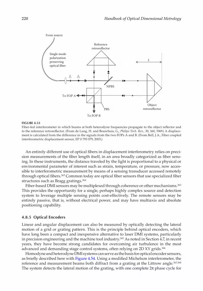
220 Handbook of Optical Dimensional Metrology
An entirely different use of optical fibers in displacement interferometry relies on preci-sion measurements of the fiber length itself, in an area broadly categorized as fiber sens-ing. In these instruments, the distance traveled by the light is proportional to a physical or environmental parameter of interest such as strain, temperature, or pressure, now acces-sible to interferometric measurement by means of a sensing transducer accessed remotely through optical fibers.363 Common today are optical fiber sensors that use specialized fiber structures such as Bragg gratings.364
Fiber-based DMI sensors may be multiplexed through coherence or other mechanisms.363 This provides the opportunity for a single, perhaps highly complex source and detection system to leverage multiple sensing points cost-effectively. The remote sensors may be entirely passive, that is, without electrical power, and may have multiaxis and absolute positioning capability.
4.8.5 Optical Encoders
Linear and angular displacement can also be measured by optically detecting the lateral motion of a grid or grating pattern. This is the principle behind optical encoders, which have long been a compact and inexpensive alternative to laser DMI systems, particularly in precision engineering and the machine tool industry.365 As noted in Section 4.7, in recent years, they have become strong candidates for overcoming air turbulence in the most advanced and demanding stage control systems, often relying on 2D XY grids.366
Homodyne and heterodyne DMI systems can serve as the basis for optical encoder sensors, as briefly described here with Figure 4.54. Using a modified Michelson interferometer, the reference and measurement beams both diffract from a grating at the Littrow angle.367,368 The system detects the lateral motion of the grating, with one complete 2π phase cycle for
From source
Single modepolarizationpreservingoptical fiber
To FOP A
PBS
To FOP B
Objectretroreflector
Referenceretroreflector
NPBS
L
f1 f2
FIGURE 4.53Fiber-fed interferometer in which beams at both heterodyne frequencies propagate to the object reflector and to the reference retroreflector. (From de Lang, H. and Bouwhuis, G., Philips Tech. Rev., 30, 160, 1969.) A displace-ment is calculated from the difference in the signals from the two FOPs A and B. (From Bell, J.A., Fiber coupled interferometric displacement sensor, EP 0 793 079, 2003.)

221Displacement Measuring Interferometry
each lateral displacement equal to half the grating period. Modern systems target sub-nanometer resolution and can have the benefit of reduced sensitivity to air turbulence.369 The configuration of Figure 4.54 is also sensitive to grating tilt, because of the wide separa-tion of the points of optical contact for the grating reference and measurement beam, and is useful for monitoring this degree of freedom. Designs have been developed specifically for lateral motions only, with tolerance for tip and tilt, using the same basic double-pass principles as an HSPMI.370–372
4.9 Summary: Using Displacement Interferometry
Throughout this survey, consistent themes characterize laser displacement interferometry as an option for precision position monitoring. Chief among this is high resolution (to <1 nm) over wide displacement ranges (>1 m typically, >1 km for geophysical and space applica-tions), low Abbe error, and high-speed data acquisition (Sections 4.1 and 4.2). Applications that rely on these favorable characteristics include microlithography stage position control, machine tool validation, and the calibration of secondary position sensors (Section 4.7). These benefits are offset by the relative high cost of laser interferometry compared to other options, sensitivity to air turbulence, and absence of absolute distance information for the most common commercial systems.
Assuming that the application calls for a displacement interferometer, there are addi-tional choices regarding the configuration and the necessary enabling elements to pro-vide the desired position data. Configuration choices include homodyne or heterodyne method detection (Section 4.3), Zeeman or externally modulated light source (Section 4.4), and the geometry for the interferometer optics (Section 4.5). The choice of inter-ferometer components and system combined with the environmental conditions and the measurement strategy will determine the level of uncertainty (Section 4.6) and dictate modifications or upgrades based on the magnitudes of the various uncertainty contributions.
The advancing requirements for applications continue to drive the advancement of new displacement interferometer systems. Developing solutions (Section 4.8) seek to overcome
From source To detector
PBS
Grating
FIGURE 4.54Optical encoder for detecting lateral motions of a grating using a Michelson interferometer. (From Akiyama, K. and Iwaoka, H., High resolution digital diffraction grating scale encoder, U.S. Patent 4,629,886, 1986.)
222 Handbook of Optical Dimensional Metrology
traditional limitations as well as to push the technology to new performance targets. These developments provide opportunities for innovation as well as new applications for what is arguably the most fundamental and historical application of optical interference in precision engineering.
References
1. G. R. Harrison and G. W. Stroke, Interferometric control of grating ruling with continuous car-riage advance, Journal of the Optical Society of America 45, 112–121 (1955).
2. A. A. Michelson, Comparison of the international metre with the wavelength of the light of cadmium, Astronomy and Astro-Physics 12, 556–560 (1893).
3. R. Benoît, Application des phénomènes d’interférence a des déterminations métrologique, Journal de Physique Théorique et Appliquée 7, 57–68 (1898).
4. S. P. Poole and J. H. Dowell, Application of interferometry to the routine measurement of block gauges, in Optics and Metrology, P. Mollet, ed. (Pergamon Press, New York, 405–419, 1960).
5. D. C. Barnes and M. J. Puttock, National physics laboratory interferometer, The Engineer 196, 763–766 (1953).
6. D. Malacara, M. Servín, and Z. Malacara, Signal phase detection, in Interferogram Analysis for Optical Testing (Marcel Dekker, Inc., New York, pp. 113–168, 1998).
7. E. R. Peck, A new principle in interferometer design, Journal of the Optical Society of America 38, 66 (1948).
8. R. Smythe and R. Moore, Instantaneous phase measuring interferometry, Optical Engineering 23, 361–364 (1984).
9. P. L. M. Heydemann, Determination and correction of quadrature fringe measurement errors in interferometers, Applied Optics 20, 3382–3384 (1981).
10. P. J. de Groot, Homodyne interferometric receiver and calibration method having improved accuracy and functionality, U.S. Patent 5,663,793 (1997).
11. M. J. Downs and K. W. Raine, An unmodulated bi-directional fringe-counting interferometer system for measuring displacement, Precision Engineering 1, 85–88 (1979).
12. A. Dorsey, R. J. Hocken, and M. Horowitz, A low cost laser interferometer system for machine tool applications, Precision Engineering 5, 29–31 (1983).
13. K. Taniguchi, H. Tsuchiya, and M. Toyama, Optical instrument for measuring displacement, U.S. Patent 4,676,645 (1987).
14. S. E. Jones, Unique advanced homodyne laser interferometer system provides a cost- effective and simple position feedback solution for precision motion control applications, in SPIE Proceedings, Photomask and Next-Generation Lithography Mask Technology XI, Yokohama, Japan, Vol. 5446, pp. 689–697 (2004).
15. H. de Lang and G. Bouwhuis, Displacement measurements with a laser interferometer, Philips Technical Review 30, 160–165 (1969).
16. J. N. Dukes and G. B. Gordon, A two-hundred-foot yardstick with graduations every micro-inch, Hewlett-Packard Journal 21, 2–8 (1970).
17. G. E. Sommargren, A new laser measurement system for precision metrology, Precision Engineering 9, 179–184 (1987).
18. F. C. Demarest, High-resolution, high-speed, low data age uncertainty, heterodyne displacement measuring interferometer electronics, Measurement Science and Technology 9, 1024–1030 (1998).
19. L. L. Deck, High-performance multi-channel fiber-based absolute distance measuring interferometer system, in SPIE Proceedings, Instrumentation, Metrology, and Standards for Nanomanufacturing III, San Diego, CA, Vol. 7405, pp. 74050E-1–74050E-9 (2009).

223Displacement Measuring Interferometry
20. P. de Groot, L. L. Deck, and C. Zanoni, Interferometer system for monitoring an object, U.S. Patent 7,826,064 (2010).
21. A. D. White and J. D. Rigden, Continuous gas maser operation in the visible, Proceedings IRE 50, 1697 (1962).
22. D. A. Shaddock, Space-based gravitational wave detection with LISA, Classical and Quantum Gravity 25, 114012 (2008).
23. D. A. Shaddock, An overview of the laser interferometer space antenna, Publications of the Astronomical Society of Australia 26, 128–132 (2009).
24. T. J. Quinn, Practical realization of the definition of the metre, including recommended radia-tions of other optical frequency standards (2001), Metrologia 40, 103–133 (2003).
25. S. J. Bennett, Length and displacement measurement by laser interferometry, in Optical Transducers and Techniques in Engineering Measurement A.R. Lunmoore, ed. (Applied Science Publishers, London, U.K., pp. 135–159, 1983).
26. The He-Ne Laser, in Springer Handbook of Lasers and Optics, F. Träger, ed. (Springer Verlag, Berlin, Germany, pp. 756–757, 2007).
27. J. A. Stone, J. E. Decker, P. Gill, P. Juncar, A. Lewis, G. D. Rovera, and M. Viliesid, Advice from the CCL on the use of unstabilized lasers as standards of wavelength: The helium-neon laser at 633 nm, Metrologia 46, 11–18 (2009).
28. H. Boersch, H. Eichler, and W. Wiesemann, Measurement of length shifts down to 10−3 Å with a two-mode laser, Applied Optics 9, 645–648 (1970).
29. M.-S. Kim and S.-W. Kim, Two-longitudinal-mode He-Ne laser for heterodyne interferometers to measure displacement, Applied Optics 41, 5938–5942 (2002).
30. S. Yokoyama, T. Yokoyama, and T. Araki, High-speed subnanometre interferometry using an improved three-mode heterodyne interferometer, Measurement Science and Technology 16, 1841–1847 (2005).
31. G. M. Burgwald and W. P. Kruger, An instant-on laser for length measurement, Hewlett-Packard Journal 21, 14–16 (1970).
32. T. Baer, F. V. Kowalski, and J. L. Hall, Frequency stabilization of a 0.633-μm He-Ne longitudinal Zeeman laser, Applied Optics 19, 3173–3177 (1980).
33. R. C. Quenelle and L. J. Wuerz, A new microcomputer-controlled laser dimensional measure-ment and analysis system, Hewlett-Packard Journal 34, 3–13 (1983).
34. I. Tobias, M. L. Skolnick, R. A. Wallace, and T. G. Polanyi, Derivation of a frequency-sensitive signal from a gas laser in an axial magnetic field, Applied Physics Letters 6, 198–200 (1965).
35. P. Zeeman, On the influence of magnetism on the nature of the light emitted by a substance, The Astrophysical Journal 5, 332–347 (1897).
36. R. H. Morris, J. B. Ferguson, and J. S. Warniak, Frequency stabilization of internal mirror He-Ne lasers in a transverse magnetic field, Applied Optics 14, 2808 (1975).
37. H. Takasaki, N. Umeda, and M. Tsukiji, Stabilized transverse Zeeman laser as a new light source for optical measurement, Applied Optics 19, 435–441 (1980).
38. N. Umeda, M. Tsukiji, and H. Takasaki, Stabilized 3He-20Ne transverse Zeeman laser, Applied Optics 19, 442–450 (1980).
39. L. L. Deck and M. L. Holmes, Optical frequency stabilization of a compact heterodyne source for an industrial distance measuring interferometer system, in Proceedings of the 1999 Annual Meeting of the American Society for Precision Engineering, Raleigh, NC, Vol. 20, pp. 477–480 (1999).
40. L. L. Deck, Frequency stabilized laser system, U.S. Patent 6,434,176 (2002). 41. R. J. Hocken and H. P. Layer, Lasers for dimensional measurement, Annals of the CIRP
28, 303–306 (1979). 42. ZMI™ 7705 Laser Head, Specification Sheet SS-0044 (Zygo Corporation, Middlefield, CT, 2009). 43. M. J. Downs, Optical metrology: The precision measurement of displacement using optical
interferometry, in From instrumentation to nanotechnology, 1st edn., J. W. Gardner and H. T. Hingle, eds. (CRC Press, Boca Raton, FL, pp. 213–226, 1992).

224 Handbook of Optical Dimensional Metrology
44. A. D. White and L. Tsufura, Helium-neon lasers, in Handbook of Laser Technology and Applications Volume II: Laser Design and Laser Systems, C. E. Webb and J. D. C. Jones, eds. (Institute of Physics, London, U.K., pp. 1399, 2004).
45. Y. Xie and Y.-Z. Wu, Elliptical polarization and nonorthogonality of stabilized Zeeman laser output, Applied Optics 28, 2043–2046 (1989).
46. D. J. Lorier, B. A. W. H. Knarren, S. J. A. G. Cosijns, H. Haitjema, and P. H. J. Schellekens, Laser polarization state measurement in heterodyne interferometry, CIRP Annals—Manufacturing Technology 52, 439–442 (2003).
47. G. E. Sommargren, Apparatus to transform a single frequency, linearly polarized laser beam into a beam with two, orthogonally polarized frequencies, U.S. Patent 4,684,828 (1987).
48. G. E. Sommargren and M. Schaham, Heterodyne interferometer system, U.S. Patent 4,688,940 (1987).
49. P. Dirksen, J. v. d. Werf, and W. Bardoel, Novel two-frequency laser, Precision Engineering 17, 114–116 (1995).
50. R. Balhorn, H. Kunzmann, and F. Lebowsky, Frequency stabilization of internal-mirror Helium-Neon lasers, Applied Optics 11, 742–744 (1972).
51. S. J. Bennett, R. E. Ward, and D. C. Wilson, Comments on: Frequency stabilization of internal mirror He-Ne lasers, Applied Optics 12, 1406–1406 (1973).
52. ZMI™ 7724 Laser head Specification Sheet, SS-0081 (Zygo Corporation, Middlefield, CT, 2009). 53. Optics and Laser Heads for Laser-Interferometer Positioning Systems: Product Overview, 5964–6190E
(Agilent Technologies, Santa Clara, CA, 2009). 54. J. Koning and P. H. J. Schellekens, Wavelength stability of He-Ne lasers used in interferometry:
Limitations and traceability, Annals of the CIRP 28, 307–310 (1979). 55. S. N. Lea, W. R. C. Rowley, H. S. Margolis, G. P. Barwood, G. Huang, P. Gill, J.-M. Chartier, and
R. S. Windeler, Absolute frequency measurements of 633 nm iodine-stabilized helium–neon lasers, Metrologia 40, 84–88 (2003).
56. ZMI 7702 Laser Head (P/N 8070–0102-XX) Operating Manual, OMP-0402H (Zygo Corporation, Middlefield, CT, 2007), p. 9.
57. W.-K. Lee, H. S. Suh, and C.-S. Kang, Vacuum wavelength calibration of frequency-stabilized He-Ne lasers used in commercial laser interferometers, Optical Engineering 50, 054301–054304 (2011).
58. N. Brown, Frequency stabilized lasers: Optical feedback effects, Applied Optics 20, 3711–3714 (1981).
59. N. Bobroff, Recent advances in displacement measuring interferometry, Measurement Science and Technology 4, 907–926 (1993).
60. L. J. Aplet and J. W. Carson, A Faraday effect optical isolator, Applied Optics 3, 544–545 (1964). 61. H. A. Hill and P. de Groot, Apparatus to transform two nonparallel propagating optical beam
components into two orthogonally polarized beam components, U.S. Patent 6,236,507 (2001). 62. H. P. Layer, Acoustooptic modulator intensity servo, Applied Optics 18, 2947–2949 (1979). 63. H. A. Hill, Apparatus for generating linearly-orthogonally polarized light beams, U.S. Patent
6,157,660 (2000). 64. P. Gill, Laser interferometry for precision engineering metrology, in Optical Methods in
Engineering Metrology, D. C. Williams, ed. (Chapman & Hall, New York, pp. 179–211 1993). 65. W. R. C. Rowley, Signal strength in two-beam interferometers with laser illumination, Journal of
Modern Optics 16, 159–168 (1969). 66. ZMI™ 7722/7724 Laser Manual P/N’s: 8070–0257-xx, 8070–0277-xx, OMP-0540C (Zygo
Corporation, Middlefield, CT, 2010), pp. 12–14. 67. ZMI™ 7714 Laser Head Manual P/N’s: 8070–0278-xx, 8070–0279-xx, OMP-0541F (Zygo
Corporation, Middlefield, CT, 2011), p. 11. 68. J. Helmcke, Realization of the metre by frequency-stabilized lasers, Measurement Science and
Technology 14, 1187–1199 (2003). 69. W. Demtröder, Laser Spectroscopy: Experimental Techniques, 4th edn. Vol. 2 (Springer Verlag,
Berlin, Germany 2008).

225Displacement Measuring Interferometry
70. G. Hanes and C. Dahlstrom, Iodine hyperfine structure observed in saturated absorption at 633 nm, Applied Physics Letters 14, 362–364 (1969).
71. A. Wallard, Frequency stabilization of the helium-neon laser by saturated absorption in iodine vapour, Journal of Physics E: Scientific Instruments 5, 926–930 (1972).
72. G. Wilson, Modulation broadening of NMR and ESR line shapes, Journal of Applied Physics 34, 3276–3285 (1963).
73. W. Schweitzer Jr, E. Kessler Jr, R. Deslattes, H. Layer, and J. Whetstone, Description, perfor-mance, and wavelengths of iodine stabilized lasers, Applied Optics 12, 2927–2938 (1973).
74. W. Tuma and C. van der Hoeven, Helium-neon laser stabilized on iodine: Design and perfor-mance, Applied Optics 14, 1896–1897 (1975).
75. V. Dandawate, Frequency stability and reproducibility of iodine stabilised He-Ne laser at 633 nm, Pramana 22, 573–578 (1984).
76. H. P. Layer, A portable iodine stabilized Helium-Neon laser, IEEE Transactions on Instrumentation and Measurement 29, 358–361 (1980).
77. J. Chartier, A. Chartier, J. Labot, and M. Winters, Absolute gravimeters: Status report on the use of iodine-stabilized He-Ne lasers at 633 nm, Metrologia 32, 181–184 (1995).
78. F. Petru, B. Popela, and Z. Vesela, Iodine-stabilized He-Ne Lasers at = 633 nm of a compact con-struction, Metrologia 29, 301–307 (1992).
79. G. Popescu, J. M. Chartier, and A. Chartier, Iodine stabilized He Ne laser at = 633 nm: Design and international comparison, Optical Engineering 35, 1348–1352 (1996).
80. J. Ishikawa, Portable national length standards designed and constructed using commercially available parts, Synthesiology-English edition 2, 246–257 (2010).
81. T. Yoon, J. Ye, J. Hall, and J. M. Chartier, Absolute frequency measurement of the iodine-stabilized He-Ne laser at 633 nm, Applied Physics B: Lasers and Optics 72, 221–226 (2001).
82. J. Chartier, H. Darnedde, M. Frennberg, J. Henningsen, U. Kärn, L. Pendrill, J. Hu, J. Petersen, O. Poulsen, and P. Ramanujam, Intercomparison of Northern European 127I2-Stabilized He-Ne Lasers at = 633 nm, Metrologia 29, 331–339 (1992).
83. J. Chartier, S. Picard-Fredin, and A. Chartier, International comparison of iodine cells, Metrologia 29, 361–367 (1992).
84. T. J. Quinn, Mise en Pratique of the definition of the Metre (1992), Metrologia 30, 523–541 (1994). 85. J. Chartier and A. Chartier, I2-stabilized 633-nm He-Ne lasers: 25 years of international compar-
isons, in SPIE Proceedings, Laser Frequency Stabilization, Standards, Measurement, and Applications, San Jose, CA, Vol. 4269, pp. 123–133 (2001).
86. A. A. Madej et al., Long-term absolute frequency measurements of 633 nm iodine-stabilized laser standards at NRC and demonstration of high reproducibility of such devices in interna-tional frequency measurements, Metrologia 41, 152–160 (2004).
87. Model 100 Iodine-stabilized He-Ne laser Specification Sheet (Winters Electro-Optics Inc., Longmont, CO).
88. J. Lawall, J. M. Pedulla, and Y. Le Coq, Ultrastable laser array at 633 nm for real-time dimen-sional metrology, Review of Scientific Instruments 72, 2879–2888 (2001).
89. E. D. Baird, R. R. Donaldson, and S. R. Patterson, The laser interferometer system for the large optics diamond turning machine, UCRL-ID-134693 (1990).
90. J. Flügge and R. G. Köning, Status of the nanometer comparator at PTB, in SPIE Proceedings, Recent Developments in Traceable Dimensional Measurements, Munich, Germany, Vol. 4401, pp. 275–283 (2001).
91. Model 200 Iodine-stabilized He-Ne laser Specification Sheet (Winters Electro-Optics Inc., Longmont, CO).
92. D. W. Allan, Statistics of atomic frequency standards, Proceedings of the IEEE 54, 221–230 (1966).
93. D. W. Allan, Time and frequency (time-domain) characterization, estimation, and prediction of precision clocks and oscillators, IEEE Transactions on Ultrasonics, Ferroelectrics and Frequency Control 34, 647–654 (1987).
94. S. J. Bennett, A double-passed Michelson interferometer, Optics Communications 4, 428–430 (1972).

226 Handbook of Optical Dimensional Metrology
95. ZMI High Stability Plane Mirror Interferometer (HSPMI) Specification Sheet, SS-0050 (Zygo Corporation, Middlefield, CT, 2009).
96. C. Zanoni, Differential interferometer arrangements for distance and angle measurements: Principles, advantages and applications, VDI-Berichte 749, 93–106 (1989).
97. P. Schellekens, G. Wilkening, F. Reinboth, M. J. Downs, K. P. Birch, and J. Spronck, Measurements of the refractive index of air using interference refractometers, Metrologia 22, 279–287 (1986).
98. R. R. Baldwin, B. E. Grote, and D. A. Harland, A laser interferometer that measures straightness of travel, Hewlett-Packard Journal 25, 10–20 (1974).
99. C. Evans, M. Holmes, F. Demarest, D. Newton, and A. Stein, Metrology and calibration of a long travel stage, CIRP Annals—Manufacturing Technology 54, 495–498 (2005).
100. H. A. Hill, Polarization preserving optical systems, U.S. Patent 6,198,574 (2001). 101. P. J. de Groot, Interferometer with tilted waveplates for reducing ghost reflections, U.S. Patent
6,163,379 (2000). 102. H. A. Hill and P. de Groot, Single-pass and multi-pass interferometry systems having a dynamic
beam-steering assembly for measuring distance, angle, and dispersion, U.S. Patent 6,313,918 (2001).
103. P. J. de Groot, Interferometric apparatus and method for measuring motion along multiple axes, U.S. Patent 6,208,424 (2001).
104. P. J. de Groot and H. A. Hill, Interferometry system and method employing an angular dif-ference in propagation between orthogonally polarized input beam components, U.S. Patent 6,778,280 (2004).
105. Y. Bitou, Polarization mixing error reduction in a two-beam interferometer, Optical Review 9, 227–229 (2002).
106. M. Tanaka, T. Yamagami, and K. Nakayama, Linear interpolation of periodic error in a hetero-dyne laser interferometer at subnanometer levels (dimension measurement), IEEE Transactions on Instrumentation and Measurement 38, 552–554 (1989).
107. C. M. Wu, S. T. Lin, and J. Fu, Heterodyne interferometer with two spatial-separated polariza-tion beams for nanometrology, Optical and Quantum Electronics 34, 1267–1276 (2002).
108. H. A. Hill, Separated beam multiple degree of freedom interferometer, U.S. Patent 7,057,739 (2006).
109. K.-N. Joo, J. D. Ellis, J. W. Spronck, P. J. M. van Kan, and R. H. M. Schmidt, Simple heterodyne laser interferometer with subnanometer periodic errors, Optics Letters 34, 386–388 (2009).
110. M. Gohlke, T. Schuldt, D. Weise, U. Johann, A. Peters, and C. Braxmaier, A high sensitivity het-erodyne interferometer as a possible optical readout for the LISA gravitational reference sensor and its application to technology verification, Journal of Physics: Conference Series 154, 012030 (2009).
111. N. Bennet, Error Sources (Zygo Corporation, Middlefield, CT, 2008). 112. J. Haycocks and K. Jackson, Traceable calibration of transfer standards for scanning probe
microscopy, Precision Engineering 29, 168–175 (2005). 113. JCGM 100:2008, Evaluation of Measurement Data—Guide to the Expression of Uncertainty in
Measurement, (JCGM, 2008). 114. H. F. F. Castro and M. Burdekin, Evaluation of the measurement uncertainty of a positional error
calibrator based on a laser interferometer, International Journal of Machine Tools and Manufacture 45, 285–291 (2005).
115. H. F. F. Castro, Uncertainty analysis of a laser calibration system for evaluating the positioning accuracy of a numerically controlled axis of coordinate measuring machines and machine tools, Precision Engineering 32, 106–113 (2008).
116. D. Ren, Optical measurements of dimensional instability, PhD dissertation, University of North Carolina, Charlotte, NC (2007).
117. T. Hausotte, B. Percle, E. Manske, R. Füßl, and G. Jäger, Measuring value correction and uncer-tainty analysis for homodyne interferometers, Measurement Science and Technology 22, 094028 (2011).

227Displacement Measuring Interferometry
118. H. P. Layer and W. T. Estler, Traceability of laser interferometric length measurements, National Bureau of Standards Technical Note 1248, National Bureau of Standards, Washington, DC, 1988.
119. M. L. Eickhoff and J. L. Hall, Real-time precision refractometry: New approaches, Applied Optics 36, 1223–1234 (1997).
120. H. Fang, A. Picard, and P. Juncar, A heterodyne refractometer for air index of refraction and air density measurements, Review of Scientific Instruments 73, 1934–1938 (2002).
121. H. Barrell and J. E. Sears, The refraction and dispersion of air for the visible spectrum, Philosophical Transactions of the Royal Society A: Mathematical, Physical and Engineering Sciences 238, 1–64 (1939).
122. B. Edlén, The refractive index of air, Metrologia 2, 71–80 (1966). 123. J. C. Owens, Optical refractive index of air: Dependence on pressure, temperature and compo-
sition, Applied Optics 6, 51–59 (1967). 124. F. E. Jones, Simplified equation for calculating the refractivity of air, Applied Optics 19, 4129–
4130 (1980). 125. F. E. Jones, The refractivity of air, Journal of Research of the National Bureau of Standards 86, 27–30
(1981). 126. K. P. Birch and M. J. Downs, An updated edlén equation for the refractive index of air, Metrologia
30, 155–162 (1993). 127. K. P. Birch and M. J. Downs, Correction to the updated edlén equation for the refractive index
of air, Metrologia 31, 315–316 (1994). 128. K. P. Birch and M. J. Downs, The results of a comparison between calculated and measured
values of the refractive index of air, Journal of Physics E: Scientific Instruments 21, 694–695 (1988).
129. K. P. Birch, F. Reinboth, R. E. Ward, and G. Wilkening, The effect of variations in the refractive index of industrial air upon the uncertainty of precision length measurement, Metrologia 30, 7–14 (1993).
130. G. Bönsch and E. Potulski, Measurement of the refractive index of air and comparison with modified Edlén’s formulae, Metrologia 35, 133–139 (1998).
131. P. E. Ciddor, Refractive index of air: New equations for the visible and near infrared, Applied Optics 35, 1566–1573 (1996).
132. P. E. Ciddor, Refractive index of air: 3. The roles of CO2, H2O, and refractivity virials, Applied Optics 41, 2292–2298 (2002).
133. P. E. Ciddor, Refractive index of air: 3. The roles of CO2, H2O, and refractivity virials: Erratum, Applied Optics 41, 7036 (2002).
134. T. L. Schmitz, C. J. Evans, A. Davies, and W. T. Estler, Displacement uncertainty in interferomet-ric radius measurements, CIRP Annals—Manufacturing Technology 51, 451–454 (2002).
135. J. Hilsenrath, Tables of Thermal Properties of Gases: Comprising Tables of Thermodynamic and Transport Properties of Air, Argon, Carbon dioxide, Carbon monoxide, Hydrogen, Nitrogen, Oxygen, and Steam, United States Government Printing Office, Washington, DC, 1955.
136. R. K. Leach, Fundamental Principles of Engineering Nanometrology (Elsevier, London, U.K., p. 81, 2010).
137. K. P. Birch and M. J. Downs, Error sources in the determination of the refractive index of air, Applied Optics 28, 825–826 (1989).
138. K. P. Birch, Precise determination of refractometric parameters for atmospheric gases, Journal of the Optical Society of America A 8, 647–651 (1991).
139. W. T. Estler, High-accuracy displacement interferometry in air, Applied Optics 24, 808–815 (1985).
140. M. J. Downs, D. H. Ferriss, and R. E. Ward, Improving the accuracy of the temperature mea-surement of gases by correction for the response delays in the thermal sensors, Measurement Science and Technology 1, 717–719 (1990).
141. M. J. Downs and K. P. Birch, Bi-directional fringe counting interference refractometer, Precision Engineering 5, 105–110 (1983).

228 Handbook of Optical Dimensional Metrology
142. K. Birch, M. Downs, and D. Ferriss, Optical path length changes induced in cell windows and solid etalons by evacuation, Journal of Physics E: Scientific Instruments 21, 690–692 (1988).
143. T. Li, Design principles for laser interference refractometers, Measurement 16, 171–176 (1995). 144. M. J. Renkens and P. H. Schellekens, An accurate interference refractometer based on a perma-
nent vacuum chamber—Development and results, CIRP Annals—Manufacturing Technology 42, 581–583 (1993).
145. J. Bryan, Design and construction of an ultraprecision 84 inch diamond turning machine, Precision Engineering 1, 13–17 (1979).
146. M. Sawabe, F. Maeda, Y. Yamaryo, T. Simomura, Y. Saruki, T. Kubo, H. Sakai, and S. Aoyagi, A new vacuum interferometric comparator for calibrating the fine linear encoders and scales, Precision Engineering 28, 320–328 (2004).
147. ZMI™ Compact Wavelength Compensator Accessory Manual, OMP-0415F (Zygo Corporation, Middlefield, CT, 2009).
148. G. E. Sommargren, Apparatus for the measurement of the refractive index of a gas, U.S. Patent 4,733,967 (1988).
149. N. Bobroff, Residual errors in laser interferometry from air turbulence and nonlinearity, Applied Optics 26, 2676–2682 (1987).
150. Y. Shibazaki, H. Kohno, and M. Hamatani, An innovative platform for high-throughput high-accuracy lithography using a single wafer stage, in SPIE Proceedings, Optical Microlithography XXII, Vol. 7274, pp. 72741I-1–72741I-12 (2009).
151. J. Flügge, C. Weichert, H. Hu, R. Köning, H. Bosse, A. Wiegmann, M. Schulz, C. Elster, and R. D. Geckeler, Interferometry at the PTB nanometer comparator: Design, status and development, in SPIE Proceedings, Fifth International Symposium on Instrumentation Science and Technology, Shenyang, China, Vol. 7133, pp. 713346-1–713346-8 (2009).
152. J. B. Wronosky, T. G. Smith, M. J. Craig, B. R. Sturgis, J. R. Darnold, D. K. Werling, M. A. Kincy, D. A. Tichenor, M. E. Williams, and P. M. Bischoff, Wafer and reticle positioning system for the extreme ultraviolet lithography engineering test stand, in SPIE Proceedings, Emerging Lithographic Technologies IV, Santa Clara, CA, Vol. 3997, pp. 829–839 (2000).
153. J. di Regolo and U. Ummethala, A novel distance measuring interferometer for rotary-linear stage metrology with shape error removal, in Proceedings of the 2011 Annual Meeting of the American Society for Precision Engineering, Denver, CO, Vol. 52, pp. 15–18 (2011).
154. N. Bobroff, Critical alignments in plane mirror interferometry, Precision Engineering 15, 33–38 (1993).
155. Laser and Optics User’s Manual, 05517–90045 (Agilent Technologies, Santa Clara, CA, pp. 7V1–7V10, 2001).
156. R. R. Baldwin, L. E. Truhe, and D. C. Woodruff, Laser optical components for machine tool and other calibrations, Hewlett-Packard Journal 34, 14–22 (1983).
157. G. Zhang and R. Hocken, Improving the accuracy of angle measurement in machine calibration, CIRP Annals—Manufacturing Technology 35, 369–372 (1986).
158. N. M. Oldham, J. A. Kramar, P. S. Hetrick, and E. C. Teague, Electronic limitations in phase meters for heterodyne interferometry, Precision Engineering 15, 173–179 (1993).
159. ZMI 4100™ Series Measurement Board Operating Manual, OMP-0508L (Zygo Corporation, Middlefield, CT, pp. 1–8, 2010).
160. T. Schmitz and H. Kim, Monte Carlo evaluation of periodic error uncertainty, Precision Engineering 31, 251–259 (2007).
161. R. C. Quenelle, Nonlinearity in interferometer measurements, Hewlett-Packard Journal 34, 10 (1983).
162. S. Cosijns, Modeling and verifying non-linearities in heterodyne displacement interferometry, Precision Engineering 26, 448–455 (2002).
163. J. Stone and L. Howard, A simple technique for observing periodic nonlinearities in Michelson interferometers, Precision Engineering 22, 220–232 (1998).
164. S. Olyaee, T. H. Yoon, and S. Hamedi, Jones matrix analysis of frequency mixing error in three-longitudinal-mode laser heterodyne interferometer, IET Optoelectronics 3, 215–224 (2009).

229Displacement Measuring Interferometry
165. P. de Groot, Jones matrix analysis of high-precision displacement measuring interferometers, in Proceedings of 2nd Topical Meeting on Optoelectronic Distance Measurement and Applications, ODIMAP II, Pavia, Italy, pp. 9–14 (1999).
166. C. M. Sutton, Non-linearity in length measurement using heterodyne laser Michelson Interferometry, Journal of Physics E: Scientific Instruments 20, 1290–1292 (1987).
167. S. Patterson and J. Beckwith, Reduction of systematic errors in heterodyne interferometric dis-placement measurement, in Proceedings of the 8th International Precision Engineering Seminar, IPES, Compiegne, France, pp. 101–104 (1995).
168. V. G. Badami and S. R. Patterson, A frequency domain method for the measurement of nonlin-earity in heterodyne interferometry, Precision Engineering 24, 41–49 (2000).
169. H. A. Hill, Tilted interferometer, U.S. Patent 6,806,962 (2004). 170. H. A. Hill, Systems and methods for quantifying nonlinearities in interferometry systems, U.S.
Patent 6,252,668 (2001). 171. C. R. Steinmetz, Sub-micron position measurement and control on precision machine tools
with laser interferometry, Precision Engineering 12, 12–24 (1990). 172. J. D. Ellis, Optical metrology techniques for dimensional stability measurements, PhD disserta-
tion, Technische Universiteit Delft, Delft, The Netherlands (2010). 173. J. Stone, S. D. Phillips, and G. A. Mandolfo, Corrections for wavelength variations in preci-
sion interferometric displacement measurements, Journal of Research of the National Institute of Standards and Technology 101, 671–674 (1996).
174. E. Abbe, Messapparate für Physiker, Zeitschrift für Instrumentenkunde 10, 446–448 (1890). 175. J. B. Bryan, The Abbé principle revisited: An updated interpretation, Precision Engineering 1,
129–132 (1979). 176. C. D. Craig and J. C. Rose, Simplified derivation of the properties of the optical center of a cor-
ner cube, Applied Optics 9, 974–975 (1970). 177. T. A. M. Ruijl and J. van Eijk, A novel ultra precision CMM based on fundamental design
principles, in Proceedings of the ASPE Topical Meeting on Coordinate Measuring Machines, Vol. 29, pp. 33–38 (2003).
178. I. Widdershoven, R. L. Donker, and H. A. M. Spaan, Realization and calibration of the Isara 400 ultra-precision CMM, Journal of Physics: Conference Series 311, 012002 (2011).
179. A. Davies, C. J. Evans, R. Kestner, and M. Bremer, The NIST X-ray optics CALIBration InteRferometer (XCALIBIR), in Optical Fabrication and Testing, OSA Technical Digest, Quebec, Canada, paper OWA5 (2000).
180. J. B. Bryan and D. L. Carter, Design of a new error-corrected co-ordinate measuring machine, Precision Engineering 1, 125–128 (1979).
181. J.-A. Kim, J. W. Kim, C.-S. Kang, J. Jin, and T. B. Eom, An interferometric calibration system for various linear artefacts using active compensation of angular motion errors, Measurement Science and Technology 22, 075304 (2011).
182. V. G. Badami and C. D. Fletcher, Validation of the performance of a high-accuracy compact interferometric sensor, in Proceedings of the 2009 Annual Meeting of the American Society for Precision Engineering, Monterey, CA, Vol. 47, pp. 112–115 (2009).
183. G. E. Sommargren, Linear/angular displacement interferometer for wafer stage metrology, in SPIE Proceedings, Optical/Laser Microlithography II, Santa Clara, CA, Vol. 1088, pp. 268–272 (1989).
184. ZMI™ Optics Guide, OMP-0326W (Zygo Corporation, Middlefield, CT, pp. 2–12, 2010). 185. M. L. Holmes and C. J. Evans, Displacement measuring interferometry measurement uncer-
tainty, in ASPE Topical Meeting on Uncertainty Analysis in Measurement and Design, State College, PA, Vol. 33, pp. 89–94 (2004).
186. R. Kendall, A servo guided X–Y–theta stage for electron beam lithography, Journal of Vacuum Science and Technology B 9, 3019–3023 (1991).
187. H. A. Hill, Beam shear reduction in interferometry systems, U.S. Patent 7,495,770 (2009). 188. H. A. Hill, Apparatus and methods for reducing non-cyclic non-linear errors in interferometry,
U.S. Patent 7,528,962 (2009).
230 Handbook of Optical Dimensional Metrology
189. W. T. Estler, Calibration and use of optical straightedges in the metrology of precision machines, Optical Engineering 24, 372–379 (1985).
190. E. W. Ebert, Flatness measurement of mounted stage mirrors, in SPIE Proceedings, Integrated Circuit Metrology, Inspection, and Process Control III, Los Angels, CA, Vol. 1087, pp. 415–424 (1989).
191. H. A. Hill and G. Womack, Multi-axis interferometer with procedure and data processing for mirror mapping, U.S. Patent 7,433,049 (2008).
192. S. L. Mielke and F. C. Demarest, Displacement measurement interferometer error correc-tion techniques, in Proceedings of the ASPE Topical Meeting on Precision Mechanical Design and Mechatronics for Sub-50nm Semiconductor Equipment, Berkley, CA, Vol. 43, pp. 113–116 (2008).
193. S. Woo, D. Ahn, D. Gweon, S. Lee, and J. Park, Measurement and compensation of bar-mirror flatness and squareness using high precision stage, in Proceedings of the 2011 Annual Meeting of the American Society for Precision Engineering, Denver, CO, Vol. 52, pp. 566–569 (2011).
194. C. J. Evans, R. J. Hocken, and W. T. Estler, Self-calibration: Reversal, redundancy, error separa-tion, and ‘absolute testing’, CIRP Annals—Manufacturing Technology 45, 617–634 (1996).
195. J.-h. Zhang and C.-H. Menq, A linear/angular interferometer capable of measuring large angu-lar motion, Measurement Science and Technology 10, 1247–1253 (1999).
196. Disk drive servo-track writing, Hewlett-Packard, Application Note 325–11,1991. 197. W. Zhou and L. Cai, An angular displacement interferometer based on total internal reflection,
Measurement Science and Technology 9, 1647–1652 (1998). 198. M. H. Chiu, J. Y. Lee, and D. C. Su, Complex refractive-index measurement based on Fresnel’s
equations and the uses of heterodyne interferometry, Applied Optics 38, 4047–4052 (1999). 199. M. H. Chiu, J. Y. Lee, and D. C. Su, Refractive-index measurement based on the effects
of total internal reflection and the uses of heterodyne interferometry, Applied Optics 36, 2936–2939 (1997).
200. F. C. Demarest, Data age adjustments, U.S. Patent 6,597,459 (2003). 201. F. C. Demarest, Method and apparatus for providing data age compensation in an interferom-
eter, U.S. Patent 5,767,972 (1998). 202. H. J. Levinson, Principles of Lithography, Vol. 146 (SPIE Press, Bellingham, WA, 2005). 203. R. R. Donaldson and S. R. Patterson, Design and construction of a large vertical axis diamond
turning machine (LODTM), in SPIE Proceedings, SPIE 27th Annual Technical Symposium and International Instrument Display, San Deigo, CA, Vol. 433, pp. 62–68 (1983).
204. J. R. Stoup and T. D. Doiron, Accuracy and versatility of the NIST M48 coordinate measur-ing machine, in SPIE Proceedings, Recent Developments in Traceable Dimensional Measurements Munich, Germany, Vol. 4401, pp. 136–146 (2001).
205. H. Kohno, Y. Shibazaki, J. Ishikawa, J. Kosugi, Y. Iriuchijima, and M. Hamatani, Latest per-formance of immersion scanner S620D with the Streamlign platform for the double pattern-ing generation, in SPIE Proceedings, Optical Microlithography XXIII, San Jose, CA, Vol. 7640, pp. 76401O-1–76401O-12 (2010).
206. T. Sandstrom and P. Ekberg, Mask lithography for display manufacturing, in SPIE Proceedings, 26th European Mask and Lithography Conference, Grenoble, France, Vol. 7545, pp. 75450K-1–75450K-18 (2010).
207. G. R. Harrison and J. E. Archer, Interferometric calibration of precision screws and control of ruling engines, Journal of the Optical Society of America 41, 495–503 (1951).
208. H. W. Babcock, Control of a ruling engine by a modulated interferometer, Applied Optics 1, 415–420 (1962).
209. I. R. Bartlett and P. C. Wildy, Diffraction grating ruling engine with piezoelectric drive, Applied Optics 14, 1–3 (1975).
210. R. Wiley, S. Zheleznyak, J. Olson, E. Loewen, and J. Hoose, A nanometer digital interferometric control for a stop start grating ruling engine, in Proceedings of the 1990 Annual Meeting of the American Society for Precision Engineering, Rochester, NY, USA, Vol. 2, pp. 131–134 (1990).
211. C. Palmer and E. Loewen, Diffraction Grating Handbook, 5th edn. (Newport Corporation, Irvine, CA, 2005).

231Displacement Measuring Interferometry
212. T. Kita and T. Harada, Ruling engine using a piezoelectric device for large and high-groove density gratings, Applied Optics 31, 1399–1406 (1992).
213. P. T. Konkola, Design and analysis of a scanning beam interference lithography system for pat-terning gratings with nanometer-level distortions, PhD dissertation, Massachusetts Institute of Technology, Cambridge, MA (2003).
214. M. Lercel, Controlling lithography variability: It’s no longer a question of nanometers (they are too big), in Proceedings of the ASPE Topical Meeting on Precision Mechanical Design and Mechatronics for Sub-50nm Semiconductor Equipment, Berkley, CA, Vol. 43, pp. 3–6 (2008).
215. H. Schwenke, U. Neuschaefer-Rube, T. Pfeifer, and H. Kunzmann, Optical methods for dimen-sional metrology in production engineering, CIRP Annals—Manufacturing Technology 51, 685–699 (2002).
216. ZMI™ Column Reference Interferometer (CRI), Vacuum Compatible Specification Sheet, SS-0067 (Zygo Corporation, Middlefield, CT, 2009).
217. J. Flügge, F. Riehle, and H. Kunzmann, Fundamental length metrology, Colin E. Webb and Julian D. C. Jones, in Handbook of Laser Technology and Applications: Applications, Institute of Physics Publishing, Philadelphia, p. 1723 (2004).
218. J. Hocken and B. R. Borchardt, On characterizing measuring machine technology, NBSIR 79–1752 (National Bureau of Standards, Washington, DC, 1979).
219. J. Ye, M. Takac, C. Berglund, G. Owen, and R. Pease, An exact algorithm for self-calibration of two-dimensional precision metrology stages, Precision Engineering 20, 16–32 (1997).
220. D. Musinski, Displacement-measuring interferometers provide precise metrology, Laser Focus World, 39, 80–83 (2003).
221. P. Petric, C. Bevis, M. McCord, A. Carroll, A. Brodie, U. Ummethala, L. Grella, A. Cheung, and R. Freed, Reflective electron beam lithography: A maskless ebeam direct write lithography approach using the reflective electron beam lithography concept, Journal of Vacuum Science and Technology B 28, C6C6–C6C13 (2010).
222. K. Suzuki and B. W. Smith, Microlithography: Science and Technology, Vol. 126 (CRC, Boca Raton, FL, pp. 383–464, 2007).
223. P. Ekberg, Ultra precision metrology: The key for mask lithography and manufacturing of high def-inition displays, Licentiate thesis, KTH Royal Institute of Technology, Stockholm, Sweden (2011).
224. W. Wills-Moren, H. Modjarrad, R. Read, and P. McKeown, Some aspects of the design and devel-opment of a large high precision CNC diamond turning machine, CIRP Annals—Manufacturing Technology 31, 409–414 (1982).
225. P. B. Leadbeater, M. Clarke, W. J. Wills-Moren, and T. J. Wilson, A unique machine for grinding large, off-axis optical components: the OAGM 2500, Precision Engineering 11, 191–196 (1989).
226. W. J. Wills-Moren and T. Wilson, The design and manufacture of a large CNC grinding machine for off-axis mirror segments, CIRP Annals—Manufacturing Technology 38, 529–532 (1989).
227. J. Klingman, The world’s most accurate lathe, Science and Technology Review 12–14 (2001). 228. D. H. Youden, Diamond turning achieves nanometer smoothness, Laser Focus World 26, 105–108
(1990). 229. Anon, More diamond turning machines, Precision Engineering 2, 225–227 (1980). 230. P. A. McKeown, K. Carlisle, P. Shore, and R. F. Read, Ultraprecision, high stiffness CNC grinding
machines for ductile mode grinding of brittle materials, in SPIE Proceedings, Infrared Technology and Applications, San Diego, CA, Vol. 1320, pp. 301–313 (1990).
231. W. J. Wills-Moren, K. Carlisle, P. A. McKeown, and P. Shore, Ductile regime grinding of glass and other brittle materials by the use of ultrastiff machine tools, in SPIE Proceedings, Advanced Optical Manufacturing and Testing, San Diego, CA, Vol. 1333, pp. 126–135 (1990).
232. P. Shore, P. Morantz, X. Luo, X. Tonnellier, R. Collins, A. Roberts, R. May-Miller, and R. Read, Big OptiX ultra precision grinding/measuring system, in Optical Fabrication, Testing, and Metrology II, SPIE Proceedings, Jena, Germany, Vol. 5965, pp. 59650Q-1–59650Q-8 (2005).
233. M. J. Liao, H. Z. Dai, P. Z. Zhang, and E. Salje, A laser interferometric auto-correcting system of high precision thread grinder, CIRP Annals—Manufacturing Technology 29, 309–312 (1980).

232 Handbook of Optical Dimensional Metrology
234. J. Otsuka, Precision thread grinding using a laser feedback system, Precision Engineering 11, 89–93 (1989).
235. J. Rohlin, An interferometer for precision angle measurements, Applied Optics 2, 762–763 (1963).
236. H. M. B. Bird, A computer controlled interferometer system for precision relative angle mea-surements, Review of Scientific Instruments 42, 1513–1520 (1971).
237. G. D. Chapman, Interferometric angular measurement, Applied Optics 13, 1646–1651 (1974). 238. J. R. Pekelsky and L. E. Munro, Bootstrap calibration of an autocollimator, index table and
sine bar ensemble for angle metrology, in SPIE Proceedings, Recent Developments in Traceable Dimensional Measurements III, San Diego, CA, Vol. 5879, pp. 58790D-1–58790D-17 (2005).
239. ZMI™ DPMI Accessory Manual, OMP-0223E (Zygo Corporation, Middlefield, CT, 2002). 240. J. G. Marzolf, Angle measuring interferometer, Review of Scientific Instruments 35, 1212–1215
(1964). 241. P. Shi and E. Stijns, New optical method for measuring small-angle rotations, Applied Optics
27, 4342–4344 (1988). 242. P. Shi, Y. Shi, and E. W. Stijns, New optical method for accurate measurement of large-angle
rotations, Optical Engineering 31, 2394–2400 (1992). 243. M. Ikram and G. Hussain, Michelson interferometer for precision angle measurement, Applied
Optics 38, 113–120 (1999). 244. T. Eom, D. Chung, and J. Kim, A small angle generator based on a laser angle interferometer,
International Journal of Precision Engineering and Manufacturing 8, 20–23 (2007). 245. H.-C. Liou, C.-M. Lin, C.-J. Chen, and L.-C. Chang, Cross calibration for primary angle
standards by a precision goniometer with a small angle interferometer, in Proceedings of the 2006 Annual Meeting of the American Society for Precision Engineering, Monterey, CA, Vol. 39, pp. 615–618 (2006).
246. M. V. R. K. Murty, Modification of michelson interferometer using only one cube-corner prism, Journal of the Optical Society of America 50, 83–84 (1960).
247. G. Peggs, A. Lewis, and S. Oldfield, Design for a compact high-accuracy CMM, CIRP Annals—Manufacturing Technology 48, 417–420 (1999).
248. I. Schmidt, T. Hausotte, U. Gerhardt, E. Manske, and G. Jäger, Investigations and calculations into decreasing the uncertainty of a nanopositioning and nanomeasuring machine (NPM-Machine), Measurement Science and Technology 18, 482–486 (2007).
249. J. A. Kramar, Nanometre resolution metrology with the molecular measuring machine, Measurement Science and Technology 16, 2121–2128 (2005).
250. I. Misumi, S. Gonda, Q. Huang, T. Keem, T. Kurosawa, A. Fujii, N. Hisata et al., Sub-hundred nanometre pitch measurements using an AFM with differential laser interferometers for designing usable lateral scales, Measurement Science and Technology 16, 2080–2090 (2005).
251. V. Korpelainen, J. Seppä, and A. Lassila, Design and characterization of MIKES metrological atomic force microscope, Precision Engineering 34, 735–744 (2010).
252. C. Werner, P. Rosielle, and M. Steinbuch, Design of a long stroke translation stage for AFM, International Journal of Machine Tools and Manufacture 50, 183–190 (2010).
253. J. S. Beers and W. B. Penzes, The NIST length scale interferometer, Journal of Research—National Institutes of Standards and Technology 104, 225–252 (1999).
254. R. Köning, Characterizing the performance of the PTB line scale interferometer by measur-ing photoelectric incremental encoders, in SPIE Proceedings, Recent Developments in Traceable Dimensional Measurements III, San Diego, CA, Vol. 5879, pp. 587908-1–587908-9 (2005).
255. M. Kajima and K. Minoshima, Picometer calibrator for precision linear encoder using a laser interferometer, in Quantum Electronics and Laser Science Conference, OSA Technical Digest (CD), paper JThB128 (2011).
256. D. Thompson and P. McKeown, The design of an ultra-precision CNC measuring machine, CIRP Annals—Manufacturing Technology 38, 501–504 (1989).
257. J. Flügge, Recent activities at PTB nanometer comparator, in SPIE Proceedings, Recent Developments in Traceable Dimensional Measurements II, San Diego, CA, Vol. 5190, pp. 391–399 (2003).

233Displacement Measuring Interferometry
258. R. Henselmans, Non-contact measurement machine for freeform optics, PhD dissertation, Eindhoven University of Technology, Eindhoven, the Netherlands (2009).
259. R. E. Henselmans and P. C. J. N. V. Rosielle, Free-form optical surface measuring apparatus and method, U.S. Patent 7,492,468 (2009).
260. L. A. Cacace, An optical distance sensor: Tilt robust differential confocal measurement with mm range and nm uncertainty, PhD dissertation, Eindhoven University of Technology, Eindhoven, the Netherlands (2009).
261. H. Takeuchi, K. Yosizumi, and H. Tsutsumi, Ultrahigh accurate 3-D profilometer using atomic force probe of measuring nanometer, in Proceedings of the ASPE Topical Meeting Freeform Optics: Design, Fabrication, Metrology, Assembly, Chapel Hill, NC, Vol. 29, pp. 102–107 (2004).
262. J. R. Cerino, K. L. Lewotsky, R. P. Bourgeois, and T. E. Gordon, High-precision mechanical profilometer for grazing incidence optics, in SPIE Proceedings, Current Developments in Optical Design and Optical Engineering IV, San Diego, CA, Vol. 2263, pp. 253–262 (1994).
263. T. E. Gordon, Circumferential and inner diameter metrology for the advanced X-ray astrophys-ics facility optics, in SPIE Proceedings, Advanced Optical Manufacturing and Testing, San Diego, CA, Vol. 1333, pp. 239–247 (1990).
264. M. Neugebauer, F. Lüdicke, D. Bastam, H. Bosse, H. Reimann, and C. Töpperwien, A new com-parator for measurement of diameter and form of cylinders, spheres and cubes under clean-room conditions, Measurement Science and Technology 8, 849–856 (1997).
265. J.-A. Kim, J. W. Kim, C.-S. Kang, and T. B. Eom, An interferometric Abbe-type comparator for the calibration of internal and external diameter standards, Measurement Science and Technology 21, 075109 (2010).
266. J. R. Miles, L. E. Munro, and J. R. Pekelsky, A new instrument for the dimensional characteriza-tion of piston–cylinder units, Metrologia 42, S220–S223 (2005).
267. J. A. Kramar, R. Dixson, and N. G. Orji, Scanning probe microscope dimensional metrology at NIST, Measurement Science and Technology 22, 024001 (2011).
268. S. Ducourtieux and B. Poyet, Development of a metrological atomic force microscope with mini-mized Abbe error and differential interferometer-based real-time position control, Measurement Science and Technology 22, 094010 (2011).
269. M. L. Holmes, Analysis and design of a long range scanning stage, PhD dissertation, University of North Carolina, Charlotte, NC (1998).
270. M. Holmes, R. Hocken, and D. Trumper, The long-range scanning stage: A novel platform for scanned-probe microscopy, Precision Engineering 24, 191–209 (2000).
271. S. J. Bennett, Thermal expansion of tungsten carbide gauge blocks, Metrology and Inspection 35–37, 1978.
272. M. Okaji, N. Yamada, and H. Moriyama, Ultra-precise thermal expansion measurements of ceramic and steel gauge blocks with an interferometric dilatometer, Metrologia 37, 165–171 (2000).
273. A. Takahashi, Measurement of long-term dimensional stability of glass ceramics using a high-precision line scale calibration system, International Journal of Automation Technology 5, 120–125 (2011).
274. S. R. Patterson, Dimensional stability of superinvar, in SPIE Proceedings, Dimensional Stability, San Diego, CA, Vol. 1335, pp. 53–59 (1990).
275. M. J. Dudik, P. G. Halverson, M. B. Levine, M. Marcin, R. D. Peters, and S. Shaklan, Precision cryogenic dilatometer for James Webb space telescope materials testing, in SPIE Proceedings, Optical Materials and Structures Technologies, San Diego, CA, Vol. 5179, pp. 155–164 (2003).
276. V. G. Badami and M. Linder, Ultra-high accuracy measurement of the coefficient of ther-mal expansion for ultra-low expansion materials, in SPIE Proceedings, Emerging Lithographic Technologies VI, San Jose, CA, Vol. 4688, pp. 469–480 (2002).
277. M. Okaji and H. Imai, High-resolution multifold path interferometers for dilatometric mea-surements, Journal of Physics E: Scientific Instruments 16, 1208–1213 (1983).
278. Y. Takeichi, I. Nishiyama, and N. Yamada, High-precision optical heterodyne interferometric dilatometer for determining absolute CTE of EUVL materials, in SPIE Proceedings, Emerging Lithographic Technologies IX, San Jose, CA, Vol. 5751, pp. 1069–1076 (2005).

234 Handbook of Optical Dimensional Metrology
279. Y. Takeichi, I. Nishiyama, and N. Yamada, High-precision (< 1ppb/° C) optical heterodyne inter-ferometric dilatometer for determining absolute CTE of EUVL materials, in SPIE Proceedings, Emerging Lithographic Technologies X, San Jose, CA, Vol. 6151, pp. 61511Z-1–61511Z-8 (2006).
280. S. J. Bennett, An absolute interferometric dilatometer, Journal of Physics E: Scientific Instruments 10, 525–530 (1977).
281. M. Okaji and N. Yamada, Precise, versatile interferometric dilatometer for room-temperature operation: Measurements on some standard reference materials, High Temperatures—High Pressures 29, 89–95 (1997).
282. V. G. Badami and S. R. Patterson, Device for high-accuracy measurement of dimensional changes, U.S. Patent 7,239,397 (2007).
283. V. G. Badami and S. R. Patterson, Optically balanced instrument for high accuracy measure-ment of dimensional change, U.S. Patent 7,426,039 (2008).
284. D. Ren, K. M. Lawton, and J. A. Miller, A double-pass interferometer for measurement of dimensional changes, Measurement Science and Technology 19, 025303 (2008).
285. S. Patterson, V. Badami, K. Lawton, and H. Tajbakhsh, The dimensional stability of lightly-loaded epoxy joints, in Proceedings of the 1998 Annual Meeting of the American Society for Precision Engineering, St.Louis, MO, Vol. 18, pp. 384–386 (1998).
286. K. Lawton, K. Lynn, and D. Ren, The measurement of creep of elgiloy springs with a balanced interferometer, Precision Engineering 31, 325–329 (2007).
287. A. Takahashi, Long-term dimensional stability and longitudinal uniformity of line scales made of glass ceramics, Measurement Science and Technology 21, 105301 (2010).
288. R. Smythe, Asphere interferometry powers precision lens manufacturing, Laser Focus World 42, 93–97 (2006).
289. M. F. Küchel, Interferometric measurement of rotationally symmetric aspheric surfaces, in SPIE Proceedings, Optical Measurement Systems for Industrial Inspection VI, Munich, Germany, pp. 738916-1–738916-34 (2009).
290. L. A. Selberg, Radius measurement by interferometry, Optical Engineering 31, 1961–1966 (1992). 291. X. C. de Lega, P. de Groot, and D. Grigg, Dimensional measurement of engineered parts
by combining surface profiling with displacement measuring interferometry, in Fringe 2001: Proceedings of the 4th International Workshop on Automatic Processing of Fringe Patterns, Berman, Germany, pp. 47–55 (2001).
292. P. de Groot, J. Biegen, J. Clark, X. Colonna de Lega, and D. Grigg, Optical interferometry for measurement of the geometric dimensions of industrial parts, Applied Optics 41, 3853–3860 (2002).
293. A. Olszak and J. Schmit, High-stability white-light interferometry with reference signal for real-time correction of scanning errors, Optical Engineering 42, 54–59 (2003).
294. A. Courteville, R. Wilhelm, M. Delaveau, F. Garcia, and F. de Vecchi, Contact-free on-axis metrology for the fabrication and testing of complex optical systems, in SPIE Proceedings, Optical Fabrication, Testing, and Metrology II, Jena, Germany, Vol. 5965, pp. 5965-10–596510-12 (2005).
295. R. D. Deslattes and A. Henins, X-ray to visible wavelength ratios, Physical Review Letters 31, 972–975 (1973).
296. J. Lawall and E. Kessler, Michelson interferometry with 10 pm accuracy, Review of Scientific Instruments 71, 2669–2676 (2000).
297. J. R. Lawall, Fabry-Perot metrology for displacements up to 50 mm, Journal of the Optical Society of America 22, 2786–2798 (2005).
298. M. A. Arain and G. Mueller, Design of the advanced LIGO recycling cavities, Optics Express 16, 10018–10032 (2008).
299. R. R. Baldwin, Machine tool evaluation by laser interferometer, Hewlett-Packard Journal 21, 12–13 (1970).
300. H. Schwenke, W. Knapp, H. Haitjema, A. Weckenmann, R. Schmitt, and F. Delbressine, Geometric error measurement and compensation of machines—An update, CIRP Annals—Manufacturing Technology 57, 660–675 (2008).
301. Calibration of a machine tool, Hewlett-Packard, Application Note 156–4.

235Displacement Measuring Interferometry
302. A. C. Okafor and Y. M. Ertekin, Vertical machining center accuracy characterization using laser interferometer: Part 1. Linear positional errors, Journal of Materials Processing Technology 105, 394–406 (2000).
303. A. C. Okafor and Y. M. Ertekin, Vertical machining center accuracy characterization using laser interferometer: Part 2. Angular errors, Journal of Materials Processing Technology 105, 407–420 (2000).
304. L. J. Wuerz and C. Burns, Dimensional metrology software eases calibration, Hewlett-Packard Journal 34, 4–5 (1983).
305. Calibration of a surface plate, Hewlett-Packard, Application Note 156–2. 306. J. C. Moody, How to calibrate surface plates in the plant, The Tool Engineer, 1955, 85–91
(1955). 307. J. C. Ziegert and C. D. Mize, The laser ball bar: A new instrument for machine tool metrology,
Precision Engineering 16, 259–267 (1994). 308. J. B. Bryan, A simple method for testing measuring machines and machine tools Part 1:
Principles and applications, Precision Engineering 4, 61–69 (1982). 309. N. Srinivasa, J. C. Ziegert, and C. D. Mize, Spindle thermal drift measurement using the laser
ball bar, Precision Engineering 18, 118–128 (1996). 310. H. F. F. Castro, A method for evaluating spindle rotation errors of machine tools using a laser
interferometer, Measurement 41, 526–537 (2008). 311. P. E. Klingsporn, Use of a laser interferometric displacement-measuring system for noncontact
positioning of a sphere on a rotation axis through its center and for measuring the spherical contour, Applied Optics 18, 2881–2890 (1979).
312. W. Barkman, A non-contact laser interferometer sweep gauge, Precision Engineering 2, 9–12 (1980).
313. V. Lee, Uncertainty of dimensional measurements obtained from self-initialized instruments, PhD dissertation, Clemson University, Clemson, SC (2010).
314. P. Freeman, Complete, practical, and rapid calibration of multi-axis machine tools using a laser tracker, Journal of the CMSC 2, 18–24 (2007).
315. H. Schwenke, R. Schmitt, P. Jatzkowski, and C. Warmann, On-the-fly calibration of linear and rotary axes of machine tools and CMMs using a tracking interferometer, CIRP Annals—Manufacturing Technology 58, 477–480 (2009).
316. K. Wendt, H. Schwenke, W. Bosemann, and M. Dauke, Inspection of large CMMs by sequen-tial multilateration using a single laser tracker, in Sixth International Conference and Exhibition on Laser Metrology, CMM and Machine Tool Performance (LAMDAMAP 2003), Huddersfield, UK, pp. 121–130 (2003).
317. H. Schwenke, M. Franke, J. Hannaford, and H. Kunzmann, Error mapping of CMMs and machine tools by a single tracking interferometer, CIRP Annals—Manufacturing Technology 54, 475–478 (2005).
318. W. T. Estler, K. L. Edmundson, G. N. Peggs, and D. H. Parker, Large-scale metrology—An update, CIRP Annals—Manufacturing Technology 51, 587–609 (2002).
319. G. Peggs, P. G. Maropoulos, E. Hughes, A. Forbes, S. Robson, M. Ziebart, and B. Muralikrishnan, Recent developments in large-scale dimensional metrology, Proceedings of the Institution of Mechanical Engineers, Part B: Journal of Engineering Manufacture 223, 571–595 (2009).
320. K. Lau, R. Hocken, and W. Haight, Automatic laser tracking interferometer system for robot metrology, Precision Engineering 8, 3–8 (1986).
321. B. Muralikrishnan, D. Sawyer, C. Blackburn, S. Phillips, B. Borchardt, and W. Estler, Performance evaluation of laser trackers, in Performance Metrics for Intelligent Systems Workshop, PerMIS’08, Gaithersburg, MD, pp. 149–155 (2008).
322. S. J. Bennett, The NPL 50-meter laser interferometer for the verification of geodetic tapes, Survey Review 22, 270–275 (1974).
323. T. Eom and J. Kim, Displacement measuring sensor calibration using nonlinearity free laser interferometer, in Proceedings, XVII IMEKO World Congress, Dubrovnik, Croatia, pp. 1911–1914 (2003).

236 Handbook of Optical Dimensional Metrology
324. H. Haitjema, Dynamic probe calibration in the μm region with nanometric accuracy, Precision Engineering 19, 98–104 (1996).
325. H. Haitjema and G. J. Kotte, Dynamic probe calibration up to 10 kHz using laser interferometry, Measurement 21, 107–111 (1997).
326. T. M. Niebauer, J. E. Faller, H. M. Godwin, J. L. Hall, and R. L. Barger, Frequency stability mea-surements on polarization-stabilized He-Ne lasers, Applied Optics 27, 1285–1289 (1988).
327. J. M. Chartier, J. Labot, G. Sasagawa, T. M. Niebauer, and W. Hollander, A portable iodine sta-bilized He-Ne laser and its use in an absolute gravimeter, IEEE Transactions on Instrumentation and Measurement, 42, 420–422 (1993).
328. C. R. Tilford, A fringe counting laser interferometer manometer, Review of Scientific Instruments 44, 180–182 (1973).
329. E. R. Harrison, D. J. Hatt, D. B. Prowse, and J. Wilbur-Ham, A new interferometric manometer, Metrologia 12, 115–122 (1976).
330. F. Alasia, A. Capelli, G. Cignolo, and M. Sardi, Performance of reflector-carrying floats in mer-cury manometers, Vacuum 46, 753–756 (1995).
331. T. Bosch and M. Lescure, Selected Papers on Laser Distance Measurement, SPIE Milestone Series, Vol. MS 115 (SPIE Press, Bellingham, WA, 1995).
332. W. R. Babbitt, J. A. Bell, B. A. Capron, P. J. de Groot, R. L. Hagman, J. A. McGarvey, W. D. Sherman, and P. F. Sjoholm, Method and apparatus for measuring distance to a target, U.S. Patent 5,589,928 (1996).
333. A. Biernat and G. Kompa, Powerful picosecond laser pulses enabling high-resolution pulsed laser radar, Journal of Optics 29, 225–228 (1998).
334. C. R. Tilford, Analytical procedure for determining lengths from fractional fringes, Applied Optics 16, 1857–1860 (1977).
335. G. L. Bourdet and A. G. Orszag, Absolute distance measurements by CO2 laser multiwave-length interferometry, Applied Optics 18, 225–227 (1979).
336. P. de Groot and S. Kishner, Synthetic wavelength stabilization for two-color laser-diode inter-ferometry, Applied Optics 30, 4026–4033 (1991).
337. K.-H. Bechstein and W. Fuchs, Absolute interferometric distance measurements applying a variable synthetic wavelength, Journal of Optics 29, 179–182 (1998).
338. P. de Groot, Three-color laser-diode interferometer, Applied Optics 30, 3612–3616 (1991). 339. P. Balling, P. Křen, P. Mašika, and S. A. van den Berg, Femtosecond frequency comb based dis-
tance measurement in air, Optics Express 17, 9300–9313 (2009). 340. J. Jin, J. W. Kim, C.-S. Kang, J.-A. Kim, and T. B. Eom, Thickness and refractive index measure-
ment of a silicon wafer based on an optical comb, Optics Express 18, 18339–18346 (2010). 341. K. Falaggis, D. P. Towers, and C. E. Towers, A hybrid technique for ultra-high dynamic range
interferometry, in SPIE Proceedings, Interferometry XIV: Techniques and Analysis, San Diego, CA, Vol. 7063, pp. 70630X-1–70630X-8 (2008).
342. H. Kikuta, K. Iwata, and R. Nagata, Distance measurement by the wavelength shift of laser diode light, Applied Optics 25, 2976–2980 (1986).
343. A. J. d. Boef, Interferometric laser rangefinder using a frequency modulated diode laser, Applied Optics 26, 4545–4550 (1987).
344. Z. W. Barber, W. R. Babbitt, B. Kaylor, R. R. Reibel, and P. A. Roos, Accuracy of active chirp linearization for broadband frequency modulated continuous wave radar, Applied Optics 49, 213–219 (2010).
345. M. J. Rudd, A laser doppler velocimeter employing the laser as a mixer-oscillator, Journal of Physics E: Scientific Instruments 1, 723–726 (1968).
346. S. Shinohara, A. Mochizuki, H. Yoshida, and M. Sumi, Laser doppler velocimeter using the self-mixing effect of a semiconductor laser diode, Applied Optics 25, 1417–1419 (1986).
347. P. J. de Groot, G. M. Gallatin, and S. H. Macomber, Ranging and velocimetry signal generation in a backscatter-modulated laser diode, Applied Optics 27, 4475–4480 (1988).
348. E. T. Shimizu, Directional discrimination in the self-mixing type laser Doppler velocimeter, Applied Optics 26, 4541–4544 (1987).

237Displacement Measuring Interferometry
349. D. E. T. F. Ashby and D. F. Jephcott, Measurement of plasma density using a gas laser as an infrared interferometer, Applied Physics Letters 3, 13–16 (1963).
350. P. de Groot, Range-dependent optical feedback effects on the multimode spectrum of laser diodes, Journal of Modern Optics 37, 1199–1214 (1990).
351. T. Bosch, N. l. Servagent, and S. Donati, Optical feedback interferometry for sensing applica-tion, Optical Engineering 40, 20–27 (2001).
352. A. Bearden, M. P. O’Neill, L. C. Osborne, and T. L. Wong, Imaging and vibrational analysis with laser-feedback interferometry, Optics Letters 18, 238–240 (1993).
353. H. Haitjema, Achieving traceability and sub-nanometer uncertainty using interferometric tech-niques, Measurement Science and Technology 19, 084002 4 (2008).
354. L. L. Deck, Dispersion interferometry using a doubled HeNe laser (Zygo Corporation, Middlefield, CT, Unpublished, 1999).
355. K. B. Earnshaw and E. N. Hernandez, Two-laser optical distance-measuring instrument that corrects for the atmospheric index of refraction, Applied Optics 11, 749–754 (1972).
356. A. Ishida, Two wavelength displacement-measuring interferometer using second-har-monic light to eliminate air-turbulence-induced errors, Japanese Journal of Applied Physics 28, L473–L475 (1989).
357. P. de Groot and H. A. Hill, Superheterodyne interferometer and method for compensating the refractive index of air using electronic frequency multiplication, U.S. Patent 5,838,485 (1998).
358. H. A. Hill, Apparatus and methods for measuring intrinsic optical properties of a gas, U.S. Patent 6,124,931 (2000).
359. B. Knarren, S. Cosijns, H. Haitjema, and P. Schellekens, Validation of a single fibre-fed het-erodyne laser interferometer with nanometre uncertainty, Precision Engineering 29, 229–236 (2005).
360. R. J. Chaney, Laser interferometer for measuring distance using a frequency difference between two laser beams, U.S. Patent 5,274,436 (1993).
361. J. A. Bell, B. A. Capron, C. R. Pond, T. S. Breidenbach, and D. A. Leep, Fiber coupled interfero-metric displacement sensor, EP 0 793 079 (2003).
362. K.-N. Joo, J. D. Ellis, E. S. Buice, J. W. Spronck, and R. H. M. Schmidt, High resolution het-erodyne interferometer without detectable periodic nonlinearity, Optics Express 18, 1159–1165 (2010).
363. A. D. Kersey, Interferometric optical fiber sensors for absolute measurement of displacement and strain, in SPIE Proceedings, Fiber Optic Sensors: Engineering and Applications, the Hague, Province of South Holland, the Netherlands, Vol. 1511, pp. 40–50 (1991).
364. A. Othonos and K. Kyriacos, Fiber Bragg Gratings (Artech House, Norwood, MA, 1999). 365. A. H. Slocum, Precision Machine Design (Prentice Hall, Englewood Cliffs, NJ, 1992). 366. J. Gargas, R. Dorval, D. Mansur, H. Tran, D. Carlson, and M. Hercher, A versatile XY stage with
a flexural six-degree-of-freedom fine positioner, in Proceedings of the 1995 Annual Meeting of the American Society for Precision Engineering, Austin, TX, Vol. 12, pp. 203–206 (1995).
367. K. Akiyama and H. Iwaoka, High resolution digital diffraction grating scale encoder, U.S. Patent 4,629,886 (1986).
368. C.-F. Kao, S.-H. Lu, H.-M. Shen, and K.-C. Fan, Diffractive laser encoder with a grating in littrow configuration, Japanese Journal of Applied Physics 47, 1833–1837 (2008).
369. C.-C. Wu, C.-C. Hsu, J.-Y. Lee, H.-Y. Chen, and C.-L. Dai, Optical heterodyne laser encoder with sub-nanometer resolution, Measurement Science and Technology 19, 045305 (2008).
370. W.-W. Chiang and C.-K. Lee, Wavefront reconstruction optics for use in a disk drive position measurement system, U.S. Patent 5,442,172 (1995).
371. N. Nishioki and T. Itabashi, Grating interference type displacement meter apparatus, U.S. Patent 5,035,507 (1991).
372. J. William R Trutna, G. Owen, A. B. Ray, J. Prince, E. S. Johnstone, M. Zhu, and L. S. Cutler, Littrow interferometer, U.S. Patent 7,440,113 (2008).
373. M. Okaji and H. Imai, Precise and versatile systems for dilatometric measurement of solid materials, Precision Engineering 7, 206–210 (1985).

238 Handbook of Optical Dimensional Metrology
374. P. J. de Groot, X. C. de Lega, and D. A. Grigg, Step height measurements using a combination of a laser displacement gage and a broadband interferometric surface profiler, in SPIE Proceedings, Interferometry XI: Applications, Seattle, WA, Vol. 4778, pp. 127–130 (2002).
375. R. E. Spero and S. E. Whitcomb, The laser interferometer gravitational-wave observatory (LIGO), Optics and Photonics News 6, 35–39 (1995).
376. P. de Groot, ed., Optical Metrology, Encyclopedia of Optics (Wiley-VCH Publishers, Weinheim, Germany, 2004), pp. 2085–2117.


