Embed Size (px)
Citation preview

The Astrophysical Journal, 691:277–298, 2009 January 20 doi:10.1088/0004-637X/691/1/277c© 2009. The American Astronomical Society. All rights reserved. Printed in the U.S.A.
DISSECTING THE GRAVITATIONAL LENS B1608+656. I. LENS POTENTIAL RECONSTRUCTION∗
S. H. Suyu1,2,3
, P. J. Marshall4, R. D. Blandford
1,2, C. D. Fassnacht
5, L. V. E. Koopmans
6, J. P. McKean
5,7, and
T. Treu4,8
1 Theoretical Astrophysics, 103-33, California Institute of Technology, Pasadena, CA, 91125, USA; [email protected] Kavli Institute for Particle Astrophysics and Cosmology, Stanford University, PO Box 20450, MS 29, Stanford, CA 94309, USA
3 Argelander Institut fur Astronomie, Auf dem Hugel 71, D-53121 Bonn, Germany4 Department of Physics, University of California, Santa Barbara, CA 93106-9530, USA
5 Department of Physics, University of California at Davis, 1 Shields Avenue, Davis, CA 95616, USA6 Kapteyn Astronomical Institute, University of Groningen, P.O. Box 800, 9700AV Groningen, The Netherlands
7 Max-Planck-Institut fur Radioastronomie, Auf dem Hugel 69, D-53121 Bonn, GermanyReceived 2008 April 16; accepted 2008 September 23; published 2009 January 9
ABSTRACT
Strong gravitational lensing is a powerful technique for probing galaxy mass distributions and for measuringcosmological parameters. Lens systems with extended source-intensity distributions are particularly useful for thispurpose since they provide additional constraints on the lens potential (mass distribution). We present a pixelatedapproach to modeling the lens potential and source-intensity distribution simultaneously. The method makesiterative and perturbative corrections to an initial potential model. For systems with sources of sufficient extentsuch that the separate lensed images are connected by intensity measurements, the accuracy in the reconstructedpotential is solely limited by the quality of the data. We apply this potential reconstruction technique to deepHubble Space Telescope observations of B1608+656, a four-image gravitational lens system formed by a pair ofinteracting lens galaxies. We present a comprehensive Bayesian analysis of the system that takes into accountthe extended source-intensity distribution, dust extinction, and the interacting lens galaxies. Our approach allowsus to compare various models of the components of the lens system, which include the point-spread function(PSF), dust, lens galaxy light, source-intensity distribution, and lens potential. Using optimal combinationsof the PSF, dust, and lens galaxy light models, we successfully reconstruct both the lens potential and theextended source-intensity distribution of B1608+656. The resulting reconstruction can be used as the basis ofa measurement of the Hubble constant. As an illustration of the astrophysical applications of our method, we useour reconstruction of the gravitational potential to study the relative distribution of mass and light in the lensinggalaxies. We find that the mass-to-light ratio for the primary lens galaxy is (2.0 ± 0.2)h M� L−1
B,� within theEinstein radius (3.9 h−1 kpc), in agreement with what is found for noninteracting lens galaxies at the same scales.
Key words: black hole physics – galaxies: nuclei – gravitational waves – relativity
1. INTRODUCTION
Strong gravitational lens systems provide a tool for probinggalaxy mass distributions (independent of their light profiles)and for measuring cosmological parameters (e.g., Kochaneket al. 2006, and references therein). Lens systems with extendedsource-intensity distributions are of special interest because theyprovide additional constraints on the lens potential (and hencethe surface mass density) due to surface brightness conservation.In this case, simultaneous determination of the source-intensitydistribution and the lens potential is needed. To describe ei-ther the source-intensity or the lens potential/mass distribution,there are two approaches in the literature: (1) “parametric,” orbetter, “simply parameterized,” using simple, physically mo-tivated functional forms described by a few (∼ 10) parame-ters (e.g., Kochanek; 1991; Kneib et al.; 1996; Keeton 2001;Marshall 2006; Jullo et al. 2007), and (2) pixel-based (“pixe-lated,” or “free-form,” or sometimes, inaccurately, “nonparamet-ric”) modeling on a grid, which has been done for both the sourceintensity (e.g., Wallington et al. 1996; Warren & Dye 2003;
∗ Based in part on observations made with the NASA/ESA Hubble SpaceTelescope, obtained at the Space Telescope Science Institute, which is operatedby the Association of Universities for Research in Astronomy, Inc., underNASA contract NAS 5-26555. These observations are associated with programGO-10158.8 Sloan Fellow, Packard Fellow.
Treu & Koopmans 2004; Dye & Warren 2005; Koopmans 2005;Brewer & Lewis 2006; Suyu et al. 2006; Wayth & Webster 2006;Dye et al. 2008) and the lens potential/mass distribution (e.g.,Williams & Saha 2000; Bradac et al. 2005; Koopmans 2005;Saha et al. 2006; Suyu & Blandford 2006; Jee et al. 2007; Vegetti& Koopmans 2008). Most of the developed lens modeling meth-ods are simply parameterized. In particular, for the measurementof the Hubble constant, lens potential/mass models prior to Sahaet al. (2006) have been simply parameterized because most ofthe strong lens systems with time delay measurements have onlypoint sources (as opposed to extended sources) to constrain thelens potential/mass distribution. A precise measurement of thevalue of H0 is important for testing the flat Λ-cold dark matter(CDM) model and studying dark energy. The cosmic microwavebackground (CMB) allows determination of cosmological pa-rameters with high accuracy with the exception of H0 (e.g.,Komatsu et al. 2008). An independent measurement of H0 tobetter than a few percent precision provides the single most use-ful complement to the CMB for dark energy studies (Hu 2005).
Koopmans (2005) developed a method for pixelated sourceintensity and lens potential reconstruction that is based on thepotential correction scheme proposed by Blandford et al. (2001).This pixelated potential reconstruction method is applicable tolens systems with extended source-intensity distributions. Pixel-based modeling has the advantage over simply-parameterizedmodeling in the flexibility in the parametrization. This is
277

278 SUYU ET AL. Vol. 691
especially important in complex lens systems (e.g., multicom-ponent source galaxies or multiple lens galaxies) where simply-parameterized models may become inadequate. Furthermore,pixel-based modeling has the capabilities of detecting dark mat-ter substructures (Koopmans 2005; Vegetti & Koopmans 2008).
In this paper, we present a lens modeling technique thatis similar to that of Koopmans (2005), but in a Bayesianframework to allow quantitative comparison between varioussource intensity and lens potential models. The point-spreadfunction (PSF), lens galaxy light, and dust models are alsoincorporated in this scheme. Therefore, this method providesa way to rank these data models (with the five interdependentcomponents: source-intensity distribution, lens potential, PSF,lens galaxy light, and dust) quantitatively. There are alsopropagation effects due to structures along the line of sight(LOS), but we ignore this for now and characterize this in aforthcoming paper (Paper II).
We choose to reconstruct the lens potential instead of thesurface mass density because (1) it is the quantity that directlyrelates to the cosmological parameters via the time delaysand angular diameter distance ratios and (2) the surface massdensity can, in principle, be easily obtained by differentiation.In contrast, Williams & Saha (2000) and Saha et al. (2006)pixelized the surface mass density. Since the surface massdensity over the entire lens plane is required in the integral forobtaining the lens potential, the conversion of the (finite) griddedmass density to the lens potential is not straightforward.
We apply the pixelated potential reconstruction method toB1608+656 (Myers et al. 1995), a quadruple image gravitationallens system with an extended source at zs = 1.394 (Fassnachtet al. 1996), and two interacting galaxy lenses at zd = 0.6304(Myers et al. 1995). B1608+656 is special in that it is the onlyfour-image gravitational lens systems with all three independenttime delays between the images measured with errors of only afew percent (Fassnacht et al. 1999, 2002). Thus, it providesa great opportunity to measure the Hubble constant, whichis the subject of Paper II. To obtain the Hubble constant tohigh precision, an accurate lens potential model is crucial.Koopmans & Fassnacht (1999) modeled this system usingsimply parameterized lens potentials, but did not account for thepresence of dust and the extended source intensity. Koopmanset al. (2003) improved on the simply parameterized modelingof the lens potential with the treatment of dust, the use ofa simply parameterized extended source-intensity distribution,and the inclusion of constraints from stellar dynamics. However,Suyu & Blandford (2006) showed that this most up-to-datesimply parameterized lens model in Koopmans et al. (2003) failscertain tests such as the crossing of the critical curve throughthe saddle point of the figure-eight-shaped intensity contour ofthe merging images. This suggests that the pixelated potentialmethod may be better suited than a simply parameterizedmethod for the two interacting galaxies. In this paper, wedeliver a comprehensive analysis of the B1608+656 systemthat incorporates the effects of the extended source intensity,presence of dust, and interacting lenses. The dissection ofB1608+656 allows us to study the relative distribution of massand light in the interacting lens galaxies.
The outline of the paper is as follows. In Section 2, weintroduce the pixelated potential reconstruction method. Wedemonstrate the method using simulated data in Section 3 andgeneralize the method to real data in Section 4. The remainingsections of the paper target B1608+656. In Section 5, wesummarize the Hubble Space Telescope (HST) observations of
B1608+656 and present the image processing. In Section 6,we show a pixelated potential reconstruction of B1608+656.Finally, in Section 7, we comment on the mass-to-light (M/L)ratio in B1608+656 based on the results of our lensing analysis.In Paper II, we use the resulting potential reconstruction ofB1608+656 together with a study of the lens environment toinfer the value of the Hubble constant.
Throughout this paper, we assume a flat Λ-CDM universewith Ωm = 0.26, ΩΛ = 0.74, and H0 = 100 h km s−1 Mpc−1
(Komatsu et al. 2008). For the lens and source redshifts inB1608+656, 1′′ on the sky corresponds to 4.9 h−1 kpc on thelens plane and 6.1 h−1 kpc on the source plane.
2. PIXELATED POTENTIAL RECONSTRUCTION
In the following subsections, we present the pixelated poten-tial reconstruction method. Section 2.1 contains the formalismof the method, and Section 2.2 is a practical implementation ofthe method.
2.1. Formalism for Iterative and Perturbative PotentialCorrections
The iterative and perturbative potential correction schemefor lens systems with extended sources was first suggestedby Blandford et al. (2001) and studied by Koopmans (2005),Suyu & Blandford (2006), and recently by Vegetti & Koopmans(2008). The pixelated potential reconstruction method that wepresent here is similar to that in Koopmans (2005) but differsin the numerical details and our use of Bayesian analysis,which allows for model comparison. The method in Vegetti& Koopmans (2008) is also based on Bayesian analysis andhas adaptive gridding on the source plane. In the rest of thesection, we briefly outline the theory of pixelated potentialreconstruction.
The central concept for this method is to start with aninitial lens potential model and to correct it, perturbatively anditeratively, to obtain an estimate of the true lens potential. Theinitial lens potential will usually be simply parameterized (toallow faster convergence with a smaller number of parameters)and ideally would be close to the true potential. It will thenbe refined via corrections on a grid of pixels. Obtaining theparameter values in the initial lens potential is often a nonlinearprocess; in contrast, the potential correction in each iteration isa linear inversion.
One way to think about this procedure is to observe that ina perfectly observed image, nested intensity contours in thesource plane map onto multiple regions of the image plane.Intensity is preserved by the lens and so the map is from a setof single source contours to the corresponding image contours.The only freedom that we have is to slide image points alongthe contours. Using the fact that the deflection field is curl-free effectively removes this freedom. What we describe is aprocedure to determine this map that takes into account a finitePSF, dust extinction, and source-intensity contamination by thelens galaxy light. In Paper II, we also include the influence ofpropagation effects.
To keep the formalism simple for the moment, let us ignorethe effects of the PSF, dust extinction, and lens galaxy light. Let�θ be the coordinates on the image plane and �β be the coordinateson the source plane. Let Id(�θ) be the observed image intensityof a lensed extended source, and let ψ(�θ) be an initial scaled

No. 1, 2009 DISSECTING THE GRAVITATIONAL LENS B1608+656. I. 279
surface potential model9 for the lens system. Given ψ(�θ), onecan obtain the best-fitting source-intensity distribution (e.g.,Suyu et al. 2006, and references therein). Let Is(�θ( �β)) be thesource intensity translated to the image plane via the potentialmodel, ψ(�θ), where �θ and �β are related via the lens equation�θ = �β − �∇ψ(�θ ). We define the intensity deficit (also known asthe image residual) on the image plane by
δI (�θ ) = Id(�θ) − Is(�θ( �β)). (1)
Suppose the initial lens potential model is perturbed from thetrue potential, ψ0(�θ), by δψ(�θ ):
ψ(�θ ) = ψ0(�θ) + δψ(�θ ). (2)
For a given image (fixed Id(�θ)) and the initial potential modelψ(�θ), we can relate the intensity deficit to the potential pertur-bation δψ(�θ ) by
δI (�θ ) = ∂Is( �β)
∂ �β · ∂δψ(�θ)
∂ �θ , (3)
to first order in δψ(�θ ) (see e.g., Suyu & Blandford 2006 fordetails). The source-intensity gradient ∂Is( �β)/∂ �β implicitlydepends on the potential model ψ(�θ) since the source position�β (where the gradient is evaluated) is related to ψ(�θ) via thelens equation. We can solve Equation (3) for δψ(�θ) given theintensity deficit and source-intensity gradients, update the initial(or previous iteration’s) potential model, and repeat the processof source-intensity reconstruction and potential correction untilthe potential converges to the true solution with zero intensitydeficit. In Section 2.2, we focus on solving Equation (3).
2.2. Implementation of Pixelated Potential Reconstruction
2.2.1. Probability Theory
The first step in solving Equation (3) for the potentialperturbation is to obtain the source-intensity gradients andthe intensity deficit, which appear in the correction equation.We follow Suyu et al. (2006) to obtain the source-intensitydistribution on a grid of pixels given the current iteration’slens potential model. In this source reconstruction approach,the data (observed image) are described by the vector dj, wherej = 1, . . . , Nd and Nd is the number of data pixels. The sourceintensity is described by the vector si, where i = 1, . . . , Nsand Ns is the number of source-intensity pixels. The observedimage is related to the source intensity via dj = fjisi + nj ,where fji is the so-called blurred lensing operator (mappingmatrix) that incorporates the lens potential (which governs thedeflection of light rays) and the PSF (blurring),10 and nj is thenoise in the data characterized by the covariance matrix CD. Inthe inference of si, we impose a prior on si, which can be thoughtof as “regularizing” the parameters si to avoid overfitting to thenoise in the data. Following Suyu et al. (2006), we use quadraticforms of the regularization (specifically, zeroth-order, gradient,and curvature forms of regularization). The Bayesian inferenceof the source-intensity distribution (si) given the observed image(dj) is a linear inversion and is a solved problem. Having
9 ψ includes the distance ratio.10 Dust extinction, if present, is also included in this mapping matrix fji .
obtained the source intensity, we can calculate the intensitydeficit and source-intensity gradients.
We pixelize the lens potential to allow for a flexibleparametrization scheme. To solve Equation (3), we cast itinto a matrix equation and invert the linear system. To writeEquation (3) in a matrix form, we discretize the lens potentialon a rectangular grid of Np pixels (which is less than the numberof data pixels Nd so that the potential and source-intensity pixelsare not underconstrained) and denote the potential perturbationby δψi , where i = 1, . . . , Np. The intensity deficit on the imagegrid is δIj = dj −fjisi , where j = 1, . . . , Nd (using the notationfrom source-intensity reconstruction, d, f, and s are the data vec-tor, the blurred lensing operator, and the source-intensity vector,respectively). Equation (3) now becomes
δI = tδψ + n, (4)
where t is a Nd × Np matrix, which incorporates the PSF, thesource-intensity gradient, and the gradient operator that acts onδψ (see the appendix for the explicit form of t), and n is thenoise in the data. The above equation is equivalent to
d = fs + tδψ + n. (5)
We can infer the potential corrections δψ given the datad, source intensity s, and source-intensity gradients that areencoded in t. In the inference, we impose a prior on δψ . Theposterior probability distribution is
posterior︷ ︸︸ ︷P (δψ |d, f, s, t, μ, gδψ ) =
likelihood︷ ︸︸ ︷P (d|δψ, t, f, s)
prior︷ ︸︸ ︷P (δψ |μ, gδψ )
P (d|f, s, t, μ, gδψ )︸ ︷︷ ︸evidence
,
(6)where μ and gδψ are the (fixed) strength and form of regu-larization for the potential correction inversion, and all irrele-vant (in)dependences have been dropped. Modeling the noise asGaussian, the likelihood is
P (d|δψ, t, f, s) = exp(−ED(d|δψ, t, f, s))
ZD, (7)
where
ED(d|δψ, t, f, s) = 1
2(d − fs − tδψ)TC−1
D (d − fs − tδψ)
(8)
= 1
2χ2, (9)
and ZD is the normalization for the probability. We express theprior in the following form:
P (δψ |μ, gδψ ) = exp(−μEδψ (δψ |gδψ ))
Zδψ (μ). (10)
We use quadratic forms of the regularizing function Eδψ . Inparticular, we use the curvature form of regularization (seefor example, Appendix A of Suyu et al. 2006 for an explicitexpression of the curvature form of regularization). We usethis regularization instead of the zeroth-order or gradient formsbecause the lens potential should in general be smooth, being theintegral of the surface mass density. Curvature regularization

280 SUYU ET AL. Vol. 691
in the potential corrections effectively corresponds to zeroth-order regularization in the surface mass density corrections.This implies a prior preference toward zero surface mass densitycorrections, thus suppressing the addition of mass to the initialmass model unless the data require it.
Maximizing the posterior of parameters δψ , we obtain themost probable solution
δψMP = A−1 D, (11)
where
A = B + μC,
B ≡ ∇∇ED(δψ) = tTC−1D t,
C ≡ ∇∇Eδψ (δψ),
D = tTC−1D (d − fs),
and ∇ ≡ ∂
∂δψ.
The matrices A, B, and C have dimensions Np × Np and are,by definition, the Hessians of the exponential arguments in theposterior, the likelihood, and the prior probability distributions,respectively.
As discussed in detail in, for example, MacKay (1992) andSuyu et al. (2006), the evidence is irrelevant in the first levelof inference where we maximize the posterior of parametersδψ to obtain the most probable parameters δψMP. However, theevidence is crucial for the second level of inference for modelcomparison, where a model incorporates the lens potential, PSF,and regularizations of both the source intensity and the potentialcorrection. If we assert that models are equally probable a priori,then the evidence gives the relative probability of the modelgiven the data. In other words, the ratio in the evidence valuesof two models tells us how much more probable the first modelis relative to the second model if we assume that the two modelsare a priori equally probable. Since the evidence gives only therelative probability, the data set needs to be kept the same formodel comparison.
The posterior (P (δψ |d, f, s, t, μ, gδψ )) and the evidence(P (d|f, s, t, μ, gδψ )) in Equation (6) are conditional onthe source-intensity distribution. Ideally, we would havean expression of the posterior for both s and δψ :P (s, δψ |d, f, λ, gS, t, μ, gδψ ), where λ and gS are, respectively,the strength and form of regularization for s. We would also ob-tain the evidence by marginalizing both the source-intensityand the potential correction values, P (d|f, λ, gS, t, μ, gδψ ) =∫
ds dδψ P(d|s, δψ, f, t) P (s, δψ |λ, gS, μ, gδψ ). However, dueto the iterative nature of the method (i.e., s and δψ arenot inferred simultaneously), we do not have such expres-sions for the posterior and the evidence. Pragmatically, we usethe evidence from the source reconstruction (given the cor-rections δψ), P (d|f, δψ, λ, gS), for comparing the potentialmodels, PSF, and regularizations. Specifically, after iteratingthrough the source-intensity reconstructions and lens poten-tial corrections, we use the final corrected lens potential forone last source-intensity reconstruction and use the evidencefrom this final source reconstruction for comparing models.This approximation is valid provided that the probability dis-tributions of δψ and the regularization constant are sharplypeaked at the most probable values. Suyu et al. (2006) showedthat the delta function approximation for the regularizationconstant is acceptable; simulations of the iterative potential
reconstruction method suggest that the probability of δψ af-ter the final iteration is sharply peaked. Therefore, the prob-ability of a given potential model, PSF, and form of regular-ization is P (f, gS|d) ∝ ∫
dλ dδψ P(d|f, δψ, λ, gS) P (f, gS) ∼P(d|f, ˆδψ, λ, gS)P(f, gS), where ˆδψ and λ are the most proba-ble solutions. Assuming that all models are equally probable apriori (i.e., P (f, gS) is constant), the evidence from the sourcereconstruction serves as a reasonable proxy to use for modelcomparison.
There is an uncertainty associated with the evidence valuesdue to finite source-intensity resolution as a result of the sourcepixelization. The source reconstruction region is initially chosensuch that the mapped source region on the image plane enclosesthe Einstein ring. This ensures that the source region containsthe entire source-intensity distribution. Throughout the iterativepixelated potential reconstruction, the source region and pix-elization are kept the same. In the final source reconstructionfor evidence computation, the evidence value depends on thepixelated source region because the goodness of fit on the im-age plane generally changes, especially in areas of significantintensity gradients, as one shifts the source region. To esti-mate the uncertainty in the evidence values, we perform the lastsource reconstruction for various source regions that are shiftedby a fraction of a pixel from the optimized one in the poten-tial reconstruction. The range of the resulting evidence valuesfor the various source regions then allow us to quantify the un-certainty in the evidence. In addition to the uncertainty due tosource pixelization, the evidence also depends on the amount ofregularization on δψ , which is discussed in Section 2.2.2.
2.2.2. Technicalities of the Pixelated Potential Reconstruction
Solving for the potential perturbations is very similar tosolving for the source-intensity distribution in Suyu et al. (2006)except for the following technical details.
1. In each iteration, the perturbative potential correction isobtained only in an annular region instead of over the entirelens potential grid due to the need for the source-intensitygradient (see Equation (3)) to be measurable. Since theextended source intensity is only non-negligible near theEinstein ring, we only have information about the source-intensity gradients in this region. In practice, the annularregion is the mapping of the finite source reconstructiongrid that encloses the extended source with a minimalnumber of source pixels (for computational efficiency). Theannulus of potential corrections obtained at each iterationis extrapolated for the next iteration by minimizing thecurvature in the potential corrections. This allows the shapeof the annular region to change as needed when the lenspotential gets corrected. In addition, the forms of theregularization matrix, as discussed in Appendix A of Suyuet al. (2006), are modified accordingly to take into accountthe nonrectangular reconstruction region (described in moredetail in the third point below).
2. Since Equation (5) is a perturbative equation in δψ , theinversion needs to be over-regularized to enforce a smallcorrection in each iteration. Empirically, we set the regu-larization constant, μ, at roughly the peak of the functionμEδψ (within a factor of 10), which corresponds to the valuebefore which the prior dominates. The resulting evidencevalue from the final source-intensity reconstruction weaklydepends on the value of μ, and we include this dependencein the uncertainty of the evidence value.

No. 1, 2009 DISSECTING THE GRAVITATIONAL LENS B1608+656. I. 281
3. The potential corrections are generally nonzero at theedge of the annular reconstruction region. This calls forslightly different structures of regularization compared tothose written in Appendix A in Suyu et al. (2006) forsource-intensity reconstruction (since the source grids arechosen to enclose the entire extended source such that edgepixels have nearly zero intensities). The regularizationsare still based on derivatives of δψ ; however, no patchingwith lower derivatives should be used for the edge pixelsbecause the zeroth-order regularization at the top/right edgewill incorrectly enforce the δψ values to zero in thoseareas. The absence of the lower derivative patches leadsto a singular regularization matrix,11 which is problematicfor evaluating the Bayesian evidence for lens potentialcorrection. However, since we do not use the evidencevalues to compare the forms of regularization for thepotential corrections (because we use only the curvatureform) nor to compare the lens potential and PSF model,the revised structure of regularization is acceptable. Wehave found this structure of regularization for potentialcorrections to work for various types of sources (withvarying sizes, shapes, number of components, etc.).
In the source reconstruction steps of this iterative scheme,we discover by using simulated data that over-regularizing thesource reconstruction in early iterations helps the process toconverge. This is because initial guess potentials that are sig-nificantly perturbed from the true potential often lead to highlydiscontinuous source distributions when optimally regularized(corresponding to maximal Bayesian evidence, which balancesthe goodness of fit and the prior), and over-regularization wouldgive a more regularized source-intensity gradient for the po-tential correction. Unfortunately, we do not have an objectiveway of setting this over-regularization factor for the source re-construction. Currently, at each source reconstruction iteration,we set the over-regularization factor such that the magnitude ofthe intensity deficit is at approximately the same level as thatfrom the optimally-regularized case but with a smoother source-intensity distribution for numerical derivatives. This scheme en-sures that we do not over-regularize when we are close to the truepotential. Based on simulated test runs, the recovery of the truepotential depends on the amount of over-regularization. Whenthe initial guess is far from the true potential, over-regularizationin the early iterations is crucial for convergence. We find that itis better to over-regularize in excess than in deficit. Too muchover-regularization simply leads to more iterations to converge,whereas too little over-regularization may not converge at all.
For each iteration of source-intensity reconstruction, there isalso a mask on the source plane to exclude source pixels thateither (1) are not mapped by that iteration’s lens potential on thedata grid or (2) have no neighboring pixels for the computationof numerical derivatives. We generalize the regularizing func-tion for this nonrectangular reconstruction region to have theright-most and top-most pixels (pixels adjacent to the edge oradjacent to the masked source pixels) patched with lower deriva-tives as we did for the edge pixels in Appendix A of Suyu et al.(2006). This patching ensures that the regularization matrix isnonsingular for the evaluation of the Bayesian evidence.
Based on simulated test runs, we find that a practical stoppingcriterion for the iterative procedure is to terminate when the
11 Having a singular regularization matrix (C) does not prevent one fromcalculating δψ because the matrix for inversion (A = B + μC) is, in general,nonsingular.
relative potential corrections between all image pairs are (δψ1 −δψ2)/(ψ1 − ψ2) < 0.1%, where 1 and 2 label the imagesin any pair. After this criterion is reached, further iterationsgive a negligible contribution to the predicted Fermat potentialdifferences between the images.
2.2.3. Mass-Sheet Degeneracy
The restriction to using only isophotal data implies that thepotential correction we obtain at each iteration may be affectedby the “mass-sheet degeneracy” (Falco et al. 1985). However,the addition of mass sheets is suppressed by the curvature formof the regularization for the potential correction and also by thelarge amount of over-regularization. We refer to Kochanek et al.(2006) and Paper II for a detailed description of the mass-sheetdegeneracy; here we review a few key points that are relevantfor the potential corrections. In essence, an arbitrary symmetricparaboloid, gradient sheet, and constant can be added to thepotential without changing the predicted lensed image:
ψν(�θ ) = 1 − ν
2|�θ |2 + �a · �θ + c + νψ(�θ ), (12)
where ψ(�θ ) is the original potential, ψν(�θ) is the transformedpotential, and ν, �a, and c are constants. The constants �a andc have no physical effects on the lens systems as they merelychange the origin on the source plane (which is unknowable) andchange the zero point of the potential (which is not observable).The parameter 1 − ν refers to the amount of mass sheet, whichcan be seen in the corresponding convergence transformation:κν(�θ) = (1 − ν) + νκ(�θ ). To make sure we remain “close” tothe initial potential model, we set ν = 1 and fix three points inthe corrected potential after each iteration to the correspondingvalues of the initial potential. Setting ν = 1 ensures that thesize of the extended source intensity remains approximately thesame, and the three fixed points allow us to solve for �a and c inEquation (12) to remove irrelevant gradient sheets and constantsin the reconstructed potential. We choose the three points tobe three of the four (top, left, right, and bottom) locations ofthe annular reconstruction region that are midway in thicknessbetween the annular edges. The three points are usually chosento be at places with lower surface brightness in the ring. Thistechnique of “fixing” the mass-sheet degeneracy is demonstratedin Section 2.2.4 using simulated data.
2.2.4. Summary
To summarize, the steps for the iterative and perturbative po-tential reconstruction scheme via matrices are as follows. (1)Reconstruct the source-intensity distribution given the initial(or corrected) lens potential based on Suyu et al. (2006). (2)Compute the intensity deficit and the source-intensity gradient.(3) Solve Equation (5) for the potential corrections δψ in theannulus of reconstruction. (4) Update the current potential usingEquation (2): ψnext iteration = ψcurrent iteration − δψ . (5) Transformthe corrected potential ψnext iteration via Equation (12) so thatν = 1 and the transformed corrected potential has the same val-ues as the initial potential at the three fixed points. (6) Extrapo-late the transformed corrected potential for the next iteration. (7)Interpolate the transformed corrected potential onto the resolu-tion of the data grid for the next iteration’s source reconstruction.(8) Repeat the process using the extrapolated and finely griddedreconstructed potential, and stop the process when the relativepotential correction between any pair of images is < 0.1%.

282 SUYU ET AL. Vol. 691
Figure 1. Demonstration of potential reconstruction: simulated data and potential perturbation. Left-hand panel: the simulated source-intensity distribution with anextended component (of peak intensity of 1.0 in arbitrary units) and a central point source (of intensity 3.0) on a 30 × 30 grid. The solid curves are the astroid causticsof the initial potential that consists of only the main SIE. Middle panel: the simulated image of the source-intensity distribution on the left using the true potentialconsisting of two SIEs (convolution with the Gaussian PSF and addition of noise are included, as described in the text). The solid line is the critical curve of theinitial potential and the dotted lines mark the annular region to which the source grid maps (using the mapping matrix f). Right-hand panel: the fractional potentialperturbation in the initial potential model. The Xs mark the three points where we fix the potential perturbation to zero. In both the middle and right-hand panels, theasterisk and the plus sign indicate the positions of the main SIE component and the perturbing SIE component, respectively.
Table 1The Relative Fermat Potential (φ = (�θ − �β)2/2 − ψ) Between the Four Images of the True Potential and of the Reconstructed Potential for a Few Selected Iterations
Potential φAB φCB φDB Source Position(arcsec)
True 0.141 0.234 0.437 . . .
Initial 0.172 ± 0.189 0.228 ± 0.156 0.437 ± 0.041 (2.587, 2.483) ± (0.013, 0.076)Iteration = 0 0.178 ± 0.070 0.246 ± 0.068 0.479 ± 0.010 (2.608, 2.483) ± (0.006, 0.034)Iteration = 2 0.161 ± 0.011 0.242 ± 0.010 0.471 ± 0.011 (2.623, 2.484) ± (0.005, 0.005)Iteration = 9 0.151 ± 0.006 0.244 ± 0.004 0.454 ± 0.006 (2.621, 2.484) ± (0.003, 0.002)
ν 0.96Iteration = 9 0.145 ± 0.006 0.234 ± 0.004 0.436 ± 0.006
Notes. We use the average source position of the four source positions for the computation of the Fermat potential. The four source positionsdeviate by ∼ 0.′′1 in the initial model, and agree within ∼ 0.′′005 at iteration = 9. The uncertainties in the predicted relative Fermat potential aredue to the uncertainties in the source position. The good agreement between the predicted Fermat potential values for the initial potential andthe true values is coincidental due to the use of the average source position.
3. DEMONSTRATION: POTENTIAL PERTURBATIONDUE TO AN INVISIBLE MASS CLUMP
In the previous section, we have outlined a method ofpixelated potential reconstruction. In this section, we willdemonstrate this method using simulated data with a lensconsisting of two mass components.
3.1. Simulated Data
We use singular isothermal ellipsoid (SIE) potentials(Kormann et al. 1994) to test the potential reconstructionmethod. For this demonstration, we let the lens be comprisedof two SIEs at the same redshift zd = 0.3: a main componentand a perturber. The main lens has a one-dimensional velocitydispersion of 260 km s−1, an axis ratio of 0.75, and a semimajoraxis position angle of 45◦ (from vertical in the counterclockwisedirection). The (arbitrary) origin of the coordinates is set suchthat the lens is centered at (2.′′5, 2.′′5), the center of the 5′′×5′′ im-age. The perturbing SIE is centered at (3.′′8, 2.′′5) with a velocitydispersion of 50 km s−1, axis ratio of 0.60, and semimajor axisposition angle of 70◦. The exact potential is the sum of these twoSIEs. We model the source intensity as an elliptical distributioninside the caustics at zs = 3.0 with an extended component (ofpeak intensity of 1.0 in arbitrary units) and a central point source(of intensity 3.0). This source is chosen such that the lensed im-
age resembles B1608+656. We use 100×100 image pixels eachof size 0.′′05 (typical pixel size of the HST Advanced Camera forSurveys (ACS)), 30 × 30 source pixels each of size 0.′′025, and25×25 potential pixels each of size 0.′′2. To obtain the simulateddata, we map the source-intensity distribution to the image planeusing the exact lens potential and the lens equation, convolvethe lensed image with a Gaussian PSF whose FWHM = 0.′′15,and add Gaussian noise of variance 0.015. Figure 1 shows thesimulated source in the left-hand panel and the simulated noisydata image in the middle panel. The Fermat potential differencebetween the images are listed in Table 1. The images are labeledby A, B, C, D, and their locations are (1.′′77, 1.′′02), (3.′′90, 3.′′59),(3.′′54, 1.′′26), and (1.′′34, 3.′′38), respectively.
3.2. Iterative and Perturbative Potential Corrections
We take the initial guess of the lens potential to be themain SIE component but with the position angle changed from45◦ to 40◦. This corresponds to a typical scenario where theperturbing SIE is faint/dark so that it is not detected in theimage, and hence is not incorporated in the smooth parametrizedmodel of the main SIE component. The rotation in the positionangle of the main SIE component corresponds to a situationwhere the mass of the galaxy does not strictly follow thelight, but the position angle of the lens mass distribution is
No. 1, 2009 DISSECTING THE GRAVITATIONAL LENS B1608+656. I. 283
initially adopted from the position angle of the lens galaxy light.Here and after, “initial potential” refers to this initial guess ofthe potential model (as opposed to the true/exact potential).Figure 1 shows the potential perturbation relative to the initialpotential in the right-hand panel. In obtaining this plot, the initialpotential has a constant gradient plane and offset added suchthat the top, left, and bottom midpoints in the annulus (markedby Xs in the plot) are fixed to the true potential with zeropotential perturbation (as described in the passage followingEquation (12)). In the iterative potential reconstruction process,the reconstructed potential at each iteration also has these threepoints in the annulus fixed to the initial model. The locationsof the three fixed points have no impact on recovering the truepotential when the source is extended enough to form an Einsteinring on the image plane. However, if the source is compact, thenlocations of the three points do matter and they are chosen tobe at places where the information content (image intensity) islow.
We perform 10 iterations of the perturbative potential correc-tion method outlined in Section 2.2. The iterations are labeled“PI” from 0 to 9. For each source reconstruction iteration, weadopt the curvature form of regularization and use the source-intensity reconstruction for the evaluation of the source-intensitygradients that are needed for the potential correction. The sourceinversions are over-regularized in early iterations in order to ob-tain smooth source reconstructions for evaluating the gradients.For each potential correction iteration, we use the curvatureform of regularization and set the regularization constant for thepotential reconstruction to be 10× the value of μ where μEδψ
peaks in iteration = 0. This regularization value is ∼ 108 andis used for all subsequent iterations (since we find that the peakin μEδψ changes little as the iterations proceed). For compari-son, the “optimal” regularization constant is ∼ 102 at iteration= 0 and is ∼ 107 at iteration = 9. Therefore, the potential re-construction inversions are heavily over-regularized in the earlyiterations to keep the corrections to first order; as the lens poten-tial gets corrected, the amount of over-regularization diminishesas the inversion approaches the linear regime with small inten-sity deficits. We show figures of source reconstructions andpotential corrections for some, but not all, of the iterations.
The top row of Figure 2 shows the results of PI = 0. Theover-regularized reconstructed source in the left-hand paneldoes not resemble the original source, and the (normalized)image residual in the middle-left panel shows prominent arcfeatures due to the presence of both the misaligned initial modeland the SIE potential perturbation. The reconstructed δψ in themiddle-right panel is of the same structures as the exact δψ inFigure 1, though the magnitude is smaller due to the correctionbeing a perturbative one. A plot of the image residual aftercorrection (= δ I − tδψ) continues to show arc features thoughless prominent than in the top middle-left panel in Figure 2. Thesame image residual plot with the true potential perturbation alsoshows similar arc features, which indicates that Equation (3)is indeed a perturbative equation and thus justifies the over-regularization in the potential correction step.
The second row of Figure 2 shows the results of PI = 2. Thereconstructed source in the left-hand panel better resembles theoriginal source in Figure 1. The amount of misfit in the imageresidual has decreased in the middle-left panel, signaling thatwe are correcting toward the true potential. The middle-rightpanel is the potential correction in PI = 2, and the right-handpanel is the amount of perturbation that remains after PI = 2.The amount of potential perturbation remaining is closer to zero
compared to the top row, which is a sign that the iterative methodconverges.
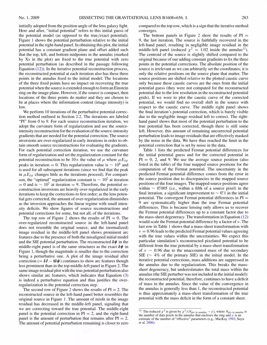
The bottom panels in Figure 2 show the results of PI =9, the last iteration. The source is faithfully recovered in theleft-hand panel, resulting in negligible image residual in themiddle-left panel (reduced χ2 = 1.02 inside the annulus12).The centroid of the source is slightly shifted compared to theoriginal because of our adding constant gradients to fix the threepoints in the potential corrections. The absolute position of thesource is irrelevant as we can arbitrarily set the coordinates; it isonly the relative positions on the source plane that matter. Thesource positions are shifted relative to the plotted caustic curveonly because these caustic curves are the ones from the initialpotential guess (they were not computed for the reconstructedpotential due to the low resolution in the reconstructed potentialgrids). If we were to plot the caustic curve of the correctedpotential, we would find no overall shift in the source withrespect to the caustic curve. The middle right panel showsthe final iteration’s potential correction, which is barely visibledue to the negligible image residual left to correct. The right-hand panel shows that most of the potential perturbation to thetrue potential has been corrected, though there is still someleft. However, this amount of remaining uncorrected potentialperturbation leads to image residuals that are effectively maskedby the noise in the data. We have thus reached the limit in thepotential correction that is set by noise in the data.
Table 1 lists the predicted Fermat potential differences forthe initial potential guess and for the corrected potential inPI = 0, 2, and 9. We use the average source position (alsolisted in the table) of the four mapped source positions for thecomputation of the Fermat potential. The uncertainty in thepredicted Fermat potential difference comes from the error inthe source position due to discrepancies in the mapped sourcepositions of the four images. The mapped source positions agreewithin ∼ 0.′′005 (i.e., within a fifth of a source pixel) in thefinal iteration, a significant improvement to ∼ 0.′′1 in the initialpotential. The convergent Fermat potential differences in PI =9 are systematically higher than the true Fermat potentialdifferences. This is because lensing only allows us to recoverthe Fermat potential differences up to a constant factor due tothe mass-sheet degeneracy. The transformation in Equation (12)would scale the Fermat potential difference by a factor of ν. Thelast row in Table 1 shows that a mass-sheet transformation withν = 0.96 leads to the predicted Fermat potential values agreeingwith the true values within the uncertainties. We expect thisparticular simulation’s reconstructed pixelated potential to bedifferent from the true potential by a mass-sheet transformationof ν ∼ 0.96 due to the unaccounted mass of the secondarySIE (∼ 4% of the primary SIE) in the initial model. In theiterative potential corrections, mass additions are suppressed inthe annulus due to the regularization. This breaks the mass-sheet degeneracy, but underestimates the total mass within theannulus (the SIE perturber was not included in the initial model):the reconstructed potential, therefore, continues to have a deficitof mass in the annulus. Since the value of the convergence inthe annulus is generally less than 1, the reconstructed potentialis thus approximately a mass-sheet transformation of the truepotential with the mass deficit in the form of a constant sheet.
12 The reduced χ2 is given by χ2/(Npix in annulus − γ ), where Npix in annulus isthe number of data pixels in the annulus that encloses the ring and γ is anestimate of the number of “effective” parameters (e.g., MacKay 1992; Suyuet al. 2006).

284 SUYU ET AL. Vol. 691
Figure 2. Demonstration of potential reconstruction: results of source-intensity reconstruction and potential correction for iteration = 0, 2, and 9. The top row showsthe results for PI = 0. Left-hand panel: the reconstructed source intensity using curvature regularization that is over-regularized to ensure a smooth resulting sourcefor evaluation of the gradients. The caustic curves in solid are those of the initial potential. Middle-left panel: the normalized image residual (difference betweenthe simulated image and the predicted image from the reconstructed source in the left-hand panel, in units of the estimated pixel uncertainty from the data imagecovariance matrix). The prominent arc features are due to the potential perturbation. Middle-right panel: the reconstructed δψ using the source-intensity gradients andimage residual. Right-hand panel: the amount of potential perturbation that remains to be corrected. The middle and bottom rows show the results for PI = 2 and PI =9, respectively, with the panels arranged in the same way as in the top row. As the iterative potential correction proceeds, the source resembles better the originalsource in Figure 1, the image residual becomes less prominent, and the magnitude of the reconstructed δψ decreases. At PI = 9, the source in the left-hand panel hasbeen faithfully reconstructed that results in negligible image residual in the middle-left panel. The remaining potential perturbation in the right-hand panel, now closeto zero, cannot be fully corrected due to the noise in the data.
The simulation we have shown is one of the worst-casescenarios where even the total mass of the initial lens modelenclosed within the Einstein ring is wrong. For initial potentialmodels that have the correct amount of mass within the Einsteinring (this enclosed mass is what lensing can robustly measureto ∼ 1%–2% accuracy in real systems) and with the mass-sheetdegeneracy broken (using external information such as stellardynamics), the reconstructed potential would faithfully recoverthe Fermat potential.
3.3. Discussion
This demonstration shows that the iterative and perturbativepotential reconstruction method works in practice. Using sim-ulated data, we find that potential perturbations � 5% (whichmay correspond to as much as ∼ 20% in the relative potentialperturbations between image pairs) are correctable, though theactual amount depends on the amount of over-regularizationfor both the source inversion and the potential correction, and
on the extendedness of the source-intensity distribution. In thecase where the solution converges, the magnitudes of the rela-tive potential corrections between image pairs steadily decrease,and we end the iterative procedure when the stopping criterion(described in Section 2.2) is met.
Regarding the size of the source-intensity distribution, themore extended a source is, the better we can recover thepotential. When the source is extended enough to be lensedinto a closed ring, the true potential can be fully recovered (upto the limit set by the noise in the data) from potential correctionsbased on Equation (5). When the source is extended to coverabout half of the Einstein ring, then the corrected potentialfaithfully reproduces the source with negligible image residual,but the relative Fermat potentials may not be recovered dueto a slight relative offset in the potential between the images.This is because the “connecting characteristics” (see Suyu &Blandford 2006) that fix the potential difference between theimages go through regions without much signal (light of thelensed source). Therefore, the potential is locally corrected at

No. 1, 2009 DISSECTING THE GRAVITATIONAL LENS B1608+656. I. 285
regions near the images (where there is light), but the globaloffset between the regions cannot be determined.
For sources that are small in extent, the potential correctionalso depends on the points we choose to fix to the initial potentialmodel. Since an isolated image is generally more prone to havingits potential be offset relative to the other images, we set twoof the three fixed points in the gaps on both sides of the mostisolated image and one point near the connecting images.
We find that a wrong PSF model (e.g., of a different width)would lead to intensity deficit that would not be correctableby the iterative potential reconstruction method. Therefore, anuncorrectable image residual is a sign that our model of thesystem (other than the lens potential) is wrong.
The potential grid that we used was 25 × 25, which we findto be a good balance between the number of degrees of freedomand goodness of fit. The higher the number of potential pixels,the better one can fit to the image residual; however, in thiscase, it is also more probable to have degenerate solutions. TheBayesian evidence from the source reconstruction in principlecan be used to compare the different potential grids. In general,we find that a potential grid that is ∼ 4 times coarser than theimage grid works well.
In Section 4, we generalize this iterative potential reconstruc-tion method, which has been shown to work on simulated data,to treat real gravitational lens images such as B1608+656.
4. GENERALIZATION TO REALISTIC DATA:INCORPORATING DUST EXTINCTION AND LENS
GALAXY LIGHT
In the previous section, we have demonstrated the method ofpixelated potential reconstruction using simulated data. In themock data, only the image of lensed source was there; in reality,there would also be light from the lens galaxy. Furthermore, insome cases, such as B1608+656, dust is present and absorbslight from both the source galaxy and the lens galaxy. Based onresults of the previous section, an accurate extraction of the lightfrom the lensed extended source is crucial for reconstructingthe lens potential. Therefore, we will generalize the formalismgiven in Section 2 to incorporate the lens galaxy light and dust.
Suppose that we have a set of PSF, dust, and lens galaxy lightmodels (the process of obtaining these models is described indetail in Section 5), a lens potential model, and the observedimage. Separating the observed image into two components, thelensed source and the lens galaxy, we can model the observedimage (as a vector for the intensities of the image pixels) as
d =lensed extended source︷ ︸︸ ︷
B · K · L · s +
lens galaxy︷ ︸︸ ︷B · K · l + n, (13)
where B is a PSF blurring matrix, K is a dust extinction matrix,L is the lensing matrix (containing the lens potential model), sis the source-intensity distribution, l is the lens galaxy intensitydistribution, and n is the noise in the data characterized bythe covariance matrix CD. This is an extended version of theequation d = fs + n in Suyu et al. (2006) with f replaced byB · K · L and d replaced by d − B · K · l . The order of the matrixproducts in both terms are obtained by tracing backwards alongthe light rays: we first encounter the PSF blurring from thetelescope (B), then dust extinction (K) in the lens plane, then thestrong lensing effects (L) in the case of the lensed source, andfinally the origin of light (s or l).
Here we assume that the dust lies in a screen in front of thelensed source and the lens galaxy. This assumption is not strictly
valid for the lens galaxy if the dust were to have originated fromG2 (Surpi & Blandford 2003). In this case, the dust and starsare mingled together in the lens galaxy. It is beyond the scope ofthis paper to treat this mixed light and dust problem. However,we note that the dust screen assumption is acceptable since theaim is to obtain an accurate lensed source-intensity distribution(for which the dust screen assumption is valid) and not the lensgalaxy intensity distribution near the core where the mixing ef-fects would dominate. Furthermore, in simple toy models, whereeither the dust and stars are uniformly mixed or the dust is ascreen lying inside the lens galaxy, we find that the extinction ofthe lens galaxy light is well approximated as extinction by a fore-ground dust screen with a reduced visual extinction. Our simpleforeground dust screen model thus provides an effective extinc-tion that incorporates the reduced extinction for the lens and thefull extinction by a foreground dust screen for the lensed source.
If the lensed source contains a bright core such as an activegalactic nucleus (AGN), then we could consider extendingEquation (13) and model the observed image as
d = B · K · L · s +Nimages∑i=1
KiαiPSF(�θi) + B · K · l + n, (14)
where the light from the extended part of the host (the first term)would be modeled separately from that from the point sources(the second term) and αi are the intensities (flux per unit solidangle in a pixel) of the point sources (which are generally not thesame for all images due to finite resolution—both lensing andmicrolensing give rise to different magnification of the point-like source—and, in the case of a time-varying core, time delaydifference). However, it is the extended image surface brightnessthat provides the information needed to reconstruct the lenspotential. For B1608+656, by taking into account the errors inthe modeling associated with the presence of the point sources(see Section 5.2.1), we will find that a separate modeling ofthe point sources is not necessary for reconstructing the lenspotential.
Given B, K, l , L, and d, one can solve for the most probablesource-intensity distribution sMP, as in Suyu et al. (2006).Furthermore, one can use the Bayesian evidence of the sourcereconstruction to rank different models of PSF, dust extinction,lens galaxy light, and lens potential (see Section 2.2.1). Whenwe compare models, we mark an annular region enclosing theEinstein ring and use the same annulus of data for all models(where models refer collectively to the lens potential, PSF, dust,lens galaxy light, and regularization). For the chosen data set, wedetermine the source region that maps to the annular region andreconstructs the source intensities in this region. The shape ofthis source region is generally not rectangular, so we generalizethe regularization schemes in Appendix A of Suyu et al. (2006)to patch the right-most and top-most pixels (pixels adjacent tothe edge of grid or adjacent to the unmapped source pixels) withlower derivatives. We will use the Bayesian evidence valuesfrom the source reconstruction in Sections 5 and 6 to comparevarious PSF, dust, lens galaxy light and lens potential modelsfor B1608+656.
To include the effects of galaxy light and dust in the pixelatedpotential reconstruction method, we incorporate K and l intoEquation (5) as in Equation (13), and include K into t (seethe Appendix for this inclusion). After these adjustments, wecan iteratively correct for the lens potential in real systemsgiven a PSF, a dust, and a lens galaxy light model based onthe machinery we developed in the previous sections.

286 SUYU ET AL. Vol. 691
Table 2HST Observations of B1608+656
Proposal Proposal Date Instrument Filter Exposures Exposure TimePI ID (s)
C. Fassnacht 10158 2004 Aug 24 ACS/WFC F606W 4 6094 646
F814W 4 6324 646
2004 Aug 25 ACS/WFC F606W 8 6098 646
F814W 8 6328 646
2004 Aug 29 ACS/WFC F606W 4 6094 646
F814W 4 6324 646
2004 Sep 17 ACS/WFC F606W 4 609F814W 4 632
4 6464 646
A. Readhead 7422 1998 Feb 7 NIC1 F160W 5 38401 20481 896
To conclude, we have outlined and demonstrated an iterativeand perturbative potential correction scheme where the accuracyin the reconstruction is limited by the noise in the data. Theinputs for this method are an initial guess of the lens potential aswell as assumptions regarding the PSF, dust, and lens galaxylight. The outputs are the reconstructed potential on a gridof pixels, the reconstructed source-intensity distribution, andthe Bayesian evidence from source reconstruction, given theassumptions. Our goal is to apply this method to the well-observed lens system B1608+656, and we begin by describingour HST observations of B1608+656 in Section 5.
5. IMAGE PROCESSING OF B1608+656
5.1. HST Observations of B1608+656
B1608+656 was observed with the ACS camera on HST inthe F606W and F814W filters in 2004 August (Proposal 10158;
PI:Fassnacht), specifically to get high signal-to-noise ratio(S/N) images of the lensed source emission. Table 2 summarizesthe observations. Each orbit of the ACS visits consisted ofone four-exposure dither pattern in either F606W or F814Wthrough the Wide Field Channel (WFC). We used the samedither pattern described in York et al. (2005) to permit drizzlingto a higher angular resolution than the default ACS CCD pixelsize (∼ 0.′′05). This subpixel scale is especially important forcharacterizing the PSF.
In order to correct for the dust extinction in the lens system,we also include the Near Infrared Camera and Multi-ObjectSpectrometer 1 (NICMOS) F160W images (Proposal 7422;PI:Readhead). Details of the NICMOS observations are alsolisted in Table 2.
The ACS images of B1608+656 are presented in Figure 3and show the two lensing galaxies and the presence of a dustlane through the system. We need to correct for both the dust
Figure 3. Left-hand (right-hand) panel: drizzled HST ACS F606W (F814W) images with 0.′′03 pixels from 9 (11) HST orbits. The dust lane and interacting galaxylenses are clearly visible. The white dots indicate the centroid positions of the images.

No. 1, 2009 DISSECTING THE GRAVITATIONAL LENS B1608+656. I. 287
lane and the light from the lens galaxies, which can affect theisophotes of the Einstein ring of the extended lensed source.Before we can determine the amount of extinction, we need tofirst unify the resolutions of the images in different wavelengthbands due to PSF dependencies. This requires PSF modeling,deconvolution, and reconvolution for images. Having unifiedthe resolutions of the images, we can determine the intrinsiccolors of the various components (lens galaxies, lensed sourcegalaxy, AGN at the core of the source galaxy) in the system thatare required for the dust correction. After correcting for dust,we can then determine the light profiles of G1 and G2 by fittingthem with Sersic profiles (I (r) ∝ exp(−(r/a)1/n), where r isthe radial coordinate, a is a scale length, and n is known as theSersic index; Sersic 1968). It is only at this stage, with the PSF,dust map, and lens galaxies’ light profiles, that we can recoverthe lensed Einstein ring surface brightness distribution for lenspotential modeling.
To execute the above plan of attack, in Section 5.2, we beginby describing the drizzling process for the ACS images that areused for the analysis. In Sections 5.3–5.5, we present a suite ofPSF, dust, and lens galaxies’ light models and describe in detailhow they are obtained. Finally, in Section 5.6, we compare thesemodels.
5.2. Image Drizzling
In the following subsections, we briefly describe the drizzlingprocess for combining the dithered ACS images and discuss thealignment of the NICMOS image to the ACS image.
5.2.1. ACS Image Processing
The ACS data were reduced using the multidrizzle package(Koekemoer et al. 2002) in an early version of the HAGGLeSimage-processing pipeline (P. J. Marshall et al. 2009, in prepa-ration), producing drizzled images with a 0.′′03 pixel scale. Thedrizzled ACS images are shown in Figure 3. The correspondingoutput weight images from multidrizzle give the values for theinverse variance of each pixel. We approximate the noise co-variance matrix as diagonal and use the variance pixel valuesfor the diagonal entries, even though drizzling will correlatethe noise between adjacent pixels. It is assumed that the effectof drizzling can be modeled as having a diagonal covariancematrix with the diagonal elements rescaled (Casertano et al.2000). In practice, we do not need to do the rescaling becausethe ranking of the models using the relative log evidence valuesfrom the source reconstruction is insensitive to rescaling of thecovariance matrix.
A pixelated representation of a continuous intensity distri-bution generally introduces error in the interpolated intensityvalues between pixels, especially for intensity distributions withsharp features. This error should be incorporated into the like-lihood function. Therefore, for modeling the source-intensitydistribution on a grid (in Sections 5.6 and 6), we also includethe error due to pixelization on the image and source planes(which we call “regridding error”) in the image covariance ma-trix. We express the regridding error on the image plane in termsof the data (instead of on the source plane and transforming itto the image plane) in order to obtain a noise map that is in-dependent of the pixelated lens modeling. The regridding errorassociated with pixel i is
(σ 2
grid
)i= 1
12μi
Δβ2
Δθ2
Nadj∑j∈ pixels adjacent to i
(dj − di)2
Nadj, (15)
where μi is the lensing magnification at pixel i, Δβ is thesource pixel size, Δθ is the image pixel size, Nadj is the numberof pixels adjacent to pixel i, and di (dj) is the image inten-sity at pixel i (j). The summation divided by Δθ2 in the aboveequation is a conservative estimate on the error due to pixeliza-tion on the image plane. Since sharper features in the imagehave larger gradients (hence, larger values for the summations),the regridding error is higher in these areas by construction. Theremaining quantities in the equation, μiΔβ2/12, account for theuncertainty in the predicted image (the source image mapped tothe image plane) due to the pixelization of the source-intensitydistribution. The factor 1/12 is the second moment of a uni-form distribution between −0.5 and 0.5. When one constructsthe predicted image by mapping each image pixel to the sourceplane and reading off the source-intensity value, the mappedsource position (of an image pixel) is generally not centeredon a source pixel, but have on average a (1/
√12)-pixel shift
from the center of the source pixel. Therefore, Δβ/√
12 is theeffective size of the source pixel, which is then magnified by(on average)
√μi due to lensing. In the pixelated potential re-
construction, we approximate the magnification at each imagepixel (which requires the second derivative of the potential) bythe value computed from the initial potential because (1) the ap-proximation enforces the regridding error to be independent ofthe pixelated potential modeling and (2) the corrected potentialvalues are obtained on an annular region only a few pixels thick.Having obtained an estimate for the regridding error, we add itin quadrature to the variance from the weight image to obtainthe entries of the approximated diagonal covariance matrix.
The inclusion of the regridding error is important for source-intensity reconstructions with sharp intensity features (such asthe presence of a bright core); it has the effect of stabilizingthe evidence values with respect to choices in the sourcepixelization. Without including the regridding error, a pixelateddescription of, for example, a source-intensity distribution witha bright core would be highly sensitive to the centering of thecore on the source pixels. A small mismatch could create largeimage residuals near the cores that would veto an otherwisegood lensing model, which has the rest of the extended featureswell described. Such an undesirable effect is mostly removed bythe inclusion of the regridding error. For B1608+656, the ratioof the regridding error to the error from the multidrizzle weightimage is around ∼ 30 near the image centroids and ∼ 1 in otherparts in the Einstein ring.
5.2.2. NICMOS Image Processing
The NICMOS F160W image was taken from Koopmanset al. (2003). Drizzled images on rectangular grids for differentinstruments are generally not on the same resolution and notaligned. This is the case for the NICMOS and ACS images. Weuse SWarp13 to align the combined NICMOS image to the ACSimages. The final SWarped NICMOS F160W image with 0.′′03pixel scales is shown in Figure 4.
5.3. PSF Modeling
In this subsection, we describe the procedure for obtainingthe PSFs for each of the ACS and the NICMOS data sets.
13 A package developed by Emmanuel Bertin at Institut d’Astrophysique deParis for resampling and coadding together FITS images.

288 SUYU ET AL. Vol. 691
5.3.1. ACS PSF
The ACS PSF is both spatially and temporally varying (e.g.,Rhodes et al. 2007). One source of temporal variation is the“breathing” of the telescope while it orbits, which causes thefocal length (and, hence, the PSF) of the telescope to change.Instead of adopting a universal PSF, we take the approach ofmodeling several PSFs using different means, and quantitativelycomparing them using the Bayesian analysis described inSection 2.2.1. This has the advantage of using the data (theobserved image) to rank the models. For each of the two drizzledACS images, we create five models for the PSF either basedon the TinyTim package (Krist & Hook 1997) or from theunsaturated stars in the field: (1) drizzled PSF (“PSF-drz”) froma set of TinyTim simulations (following Rhodes et al. 2007), (2)single (nondrizzled) TinyTim PSF (“PSF-f3”) with a telescopefocus value of −3, (3) the closest star (“PSF-C”) located at ∼ 9′′in the northeast direction from B1608+656 in the drizzled ACSfield with a Vega magnitude of 21.3 in F814W, (4) bright star #1(“PSF-B1”) that is located at ∼1.′9 southwest of B1608+656 inthe drizzled ACS field with a Vega magnitude of 18.7 in F814W,and (5) bright star #2 (“PSF-B2”) that is located at ∼ 1.′6 southof B1608+656 in the drizzled ACS field with a Vega magnitudeof 19.1.
The TinyTim frame(s) were drizzled and resampled to pixelsizes of 0.′′03 to match the resolution of the ACS images. Wekeep in mind that the TinyTim PSFs (PSF-drz and PSF-f3) maybe insufficient due to the time-varying nature of the PSF andthe aging of the detector since the TinyTim code was written.We expect the closest star to B1608+656 (PSF-C) to be agood approximation to the PSF because the spatial variationof the PSF across ∼ 9′′ should be negligible and any temporalvariations are the same as in the lens system. However, thisclosest star is not bright enough to see the secondary maximain the PSF, so we additionally include two of the brightest starsin the drizzled field mentioned above. For each of the stars inF606W and F814W, we make a small cutout around the star(25×25 pixels for PSF-C, 51×51 pixels for PSF-B1, and 41×41 pixels for PSF-B2) and center it on a 200 × 200 grid, whichis the size of the drizzled science image cutouts of B1608+656that are used for the image processing.
5.3.2. NICMOS PSF
The NICMOS PSF is thought to be more stable, and thus weassume a TinyTim model for it. The output TinyTim PSF is inthe CCD frame of NICMOS with pixel size 0.′′043. As with theF160W science image, the PSF was SWarped to be aligned withthe ACS images with 0.′′03 pixels. Since there is only one PSFmodel for NICMOS, PSF specifications throughout the rest ofthis paper refer to the ACS PSFs.
5.4. Dust Correction
With observations in two or more wavelengths, we can correctfor the dust extinction using empirical dust extinction laws.We adopt the extinction law of Cardelli et al. (1989) with thefollowing dust extinction ratios at the redshift of the lens zd =0.63 for RV = 3.1 (Galactic extinction): AF606W/AV = 1.56,AF814W/AV = 1.14, and AF160W/AV = 0.41, where Aλ isthe extinction (difference between the observed and intrinsicmagnitudes) at wavelength λ. These dust extinction ratios agreewith the values from the extinction law in Pei (1992) to within1.5%. In order to correct for the extinction, we need to knowthe intrinsic colors of the objects (details in Section 5.4.1). For
Figure 4. HST NICMOS F160W image that is SWarped to aligned to the ACSframe with a 0.′′03 pixel size. The white dots indicate the centroid positions ofthe images.
each color type of object (the lens galaxies, the source galaxy,and the AGN of source galaxy), we denote the intrinsic colorby QF = (mF,intrinsic − m1,intrinsic), where F = 1, . . . , Nb isin sequence from the reddest to the bluest wavelengths (byconstruction Q1 = 0), and Nb is the number of wavelengthbands used for dust correction. Combining the dust extinctionratios and the definition of intrinsic colors, we can modelthe observed magnitudes at each image pixel in each of thewavelength bands F in terms of AV and the intrinsic magnitudeof the reddest wavelength band m1,intrinsic as
mF ≡ mF,observed = m1,intrinsic + QF + AV kF + nF , (16)
where kF ≡ AF /AV are constants given by the extinction lawand nF is the noise in the data of wavelength band F. We cansolve for AV and m1,intrinsic at each image pixel by minimizingthe following χ2
dust for each pixel:
χ2dust =
Nb∑F=1
(mF − m1,intrinsic − QF − AV kF )2. (17)
We have weighted the images of the different bands equallybecause the uncertainty associated with mF is negligible com-pared to that of QF , and the uncertainties in QF are of comparablemagnitudes for the different bands F relative to the reddest. Thesolution that minimizes χ2
dust is
AV =[
1
Nb
(∑F
kF
)(∑F
mF
)
− 1
Nb
(∑F
kF
) (∑F
QF
)
−∑F
kF mF +∑F
kF QF
]/[
1
Nb
(∑F
kF
)2
−∑F
k2F
], (18)
No. 1, 2009 DISSECTING THE GRAVITATIONAL LENS B1608+656. I. 289
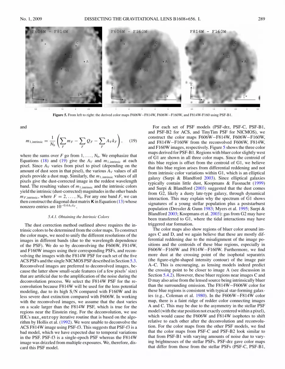
Figure 5. From left to right: the derived color maps F606W−F814W, F606W−F160W, and F814W-F160 using PSF-B1.
and
m1,intrinsic = 1
Nb
(∑F
mF −∑F
QF −∑F
AV kF
), (19)
where the sums over F go from 1, . . . , Nb. We emphasize thatEquations (18) and (19) give the AV and m1,intrinsic at eachpixel. Since AV varies from pixel to pixel (depending on theamount of dust seen in that pixel), the various AV values of allpixels provide a dust map. Similarly, the m1,intrinsic values of allpixels give the dust-corrected image in the reddest wavelengthband. The resulting values of m1,intrinsic and the intrinsic colorsyield the intrinsic (dust-corrected) magnitudes in the other bandsmF,intrinsic, where F = 2, . . . , Nb. For any one band F, we canthen construct the diagonal dust matrix K in Equation (13) whosenonzero entries are 10−0.4AV kF .
5.4.1. Obtaining the Intrinsic Colors
The dust correction method outlined above requires the in-trinsic colors to be determined from the color maps. To constructthe color maps, we need to unify the different resolutions of theimages in different bands (due to the wavelength dependenceof the PSF). We do so by deconvolving the F606W, F814W,and F160W images using their corresponding PSFs, and recon-volving the images with the F814W PSF for each set of the fiveACS PSFs and the single NICMOS PSF described in Section 5.3.Reconvolved images are preferred to deconvolved images, be-cause the latter show small-scale features (of a few pixels’ size)that are artificial due to the amplification of the noise during thedeconvolution process. We select the F814W PSF for the re-convolution because F814W will be used for the lens potentialmodeling, due to its high S/N compared with F160W and itsless severe dust extinction compared with F606W. In workingwith the reconvolved images, we assume that the dust varieson a scale larger than the F814W PSF, which is true for theregions near the Einstein ring. For the deconvolution, we useIDL’s max_entropy iterative routine that is based on the algo-rithm by Hollis et al. (1992). We were unable to deconvolve theACS F814W image using PSF-f3. This suggests that PSF-f3 is abad model, which we have expected due to temporal variationsin the PSF. PSF-f3 is a single-epoch PSF whereas the F814Wimage was drizzled from multiple exposures. We, therefore, dis-card this PSF model.
For each set of PSF models (PSF-drz, PSF-C, PSF-B1,and PSF-B2 for ACS, and TinyTim PSF for NICMOS), weconstruct the color maps F606W−F814W, F606W−F160W,and F814W−F160W from the reconvolved F606W, F814W,and F160W images, respectively. Figure 5 shows the three colormaps derived for PSF-B1. Regions with bluer color slightly westof G1 are shown in all three color maps. Since the centroid ofthis blue region is offset from the centroid of G1, we believethat this blue region arises from differential reddening and notfrom intrinsic color variations within G1, which is an ellipticalgalaxy (Surpi & Blandford 2003). Since elliptical galaxiestypically contain little dust, Koopmans & Fassnacht (1999)and Surpi & Blandford (2003) suggested that the dust comesfrom G2, likely a dusty late-type galaxy, through dynamicalinteraction. This may explain why the spectrum of G1 showssignatures of a young stellar population plus a poststarburstpopulation (Dressler & Gunn 1983; Myers et al. 1995; Surpi &Blandford 2003; Koopmans et al. 2003): gas from G2 may havebeen transferred to G1, where the tidal interactions may havetriggered star formation.
The color maps also show regions of bluer color around im-ages C and D, and we again believe that these are mostly dif-ferential reddening due to the misalignment of the image po-sitions and the centroids of these blue regions, especially inF606W−F160W and F814W−F160W. Furthermore, we findmore dust at the crossing point of the isophotal separatrix(the figure-eight-shaped intensity contour) of the image pairA–C. This is encouraging, as lensing models indeed predictthe crossing point to be closer to image A (see discussion inSection 5.4.2). However, these bluer regions near images C andD may also arise from the lensed source being intrinsically bluerthan the surrounding emission. The F814W−F606W color forthese blue regions is consistent with typical star-forming galax-ies (e.g., Coleman et al. 1980). In the F606W−F814W colormap, there is a faint ridge of redder color connecting imagesA and C. This may be due to the asymmetry in the stellar PSFmodel (with the star position not exactly centered within a pixel),which would cause the F606W and F814W isophotes to shiftrelative to each other after the deconvolution and reconvolu-tion. For the color maps from the other PSF models, we findthat the color maps from PSF-C and PSF-B2 look similar tothat from PSF-B1 with varying amounts of noise due to vary-ing brightnesses of the stellar PSFs. PSF-drz gave color mapsthat differ from those from the stellar PSFs (PSF-C, PSF-B1,

290 SUYU ET AL. Vol. 691
Figure 6. Left-hand panel: the AV map obtained from dust correction with PSF-B1 using all three bands of images and the intrinsic colors listed in Table 3. Thegalactic dust extinction law was assumed. The dust lane through images C, G2, G1, and D is visible. Right-hand panel: dust-extinction-corrected F814W image usingPSF-B1 and the three-band dust map in the left-hand panel. Compared to the right-hand panel in Figure 3, the light profile of G1 is more elliptical and the crossingpoint of the isophotal separatrix of images A and C has shifted toward A after the dust correction.
and PSF-B2) because PSF-drz, especially in the F606W band,did not exhibit a single brightness peak but a string of equalbrightness pixels at the center due to frame alignment difficultiesduring the drizzling process. This caused the brightest pixels inthe Einstein ring to shift by ∼ 1 pixel after the deconvolution andthe reconvolution process in F606W, and created artificial sharphighlights tracing the edge of the ring in the F606W−F814Wcolor map. As will be seen in Section 5.6, this leads to PSF-drzand its resulting dust map giving a lower goodness of fit in thelens inversion, and hence being ranked lower compared withother models.
In each of the color maps, we define three color regions forthe three color components: one within the Einstein ring for thelens galaxies (we assume G1 and G2 to have the same colors),one for the Einstein ring of the lensed extended source, and onefor the lensed AGN (core of the extended source). FollowingKoopmans et al. (2003), we determine the bluest color withineach region, assume that this part of the region was not absorbedby dust, and adopt this color as the intrinsic color. This assumesthat each of the three components has a constant intrinsic color.This would allow us to obtain the differential reddening for eachof the components across the lensed image; absolute reddeningis not needed because a uniform dust screen does not affect lensmodeling. Table 3 lists the intrinsic colors for each of the threepairs of color maps. The intrinsic colors of F606W−F814Ware not identical to the difference between F606W−F160W andF814W−F160W, but agree within the uncertainties (0.02–0.1).
5.4.2. Resulting Dust Maps
With the intrinsic colors determined for each PSF model, weobtain two dust maps (AV maps) using (1) only the ACS F606Wand F814W images and (2) the ACS F606W and F814W imagestogether with the NICMOS F160W image. In this way, we canassess whether the inclusion of the lower S/N NICMOS image(with the much broader PSF) improves the dust correction.
The left-hand panel of Figure 6 is the resulting AV dust mapderived using PSF-B1 and using images in all three bands. The
Figure 7. Crossing isophotes of the B1608+656 Einstein ring. Shown here isthe dust-corrected and galaxy-subtracted F814W image (solid contours), withthe critical curves of the SPLE1+D (isotropic) potential model (Koopmans et al.2003) overlaid (dashed curves). The inset shows a “zoomed-in” view of theregion between images C and A; here, the dotted curves in the zoomed-in panelare the intensity contours of the galaxy-subtracted F814W image without dustcorrection. After dust correction, the crossing point of the isophotal separatrix(the center of the figure-eight isophote) is shifted toward the critical curve,indicating successful dust correction.
dust map shows the east-west dust lane through the system(absorbing light from C, G2, G1, and D) that is visible in theoriginal drizzled ACS F606W and F814W images. There islittle extinction near images A and B, but there are faint ringssurrounding the images that are mostly due to imperfect F160Wdeconvolution. We note that the low S/N exterior to the Einsteinring results in the dust map being noisy in this area. We makesure that these noisy areas are not included in the Bayesian

No. 1, 2009 DISSECTING THE GRAVITATIONAL LENS B1608+656. I. 291
Figure 8. Sersic lens galaxy light profile fitting to the dust-corrected F814W image, with PSF-B1 and its corresponding three-band dust map, using GALFIT. Theleft-hand panel shows the best-fit Sersic light profiles with Sersic indices (nG1, nG2) = (3, 4). The middle panel shows the dust-extincted galaxy light profiles, whichis the left-hand panel with the dust extinction added back in. The right-hand panel shows image residual (difference between the F814W drizzled image in Figure 3and the middle panel) with misfit near the cores of the lens galaxies of ∼ 25%–35%.
Table 3Intrinsic Colors of the AGN, Einstein Ring, and Lens Galaxies in B1608+656
F606W−F814W F814W−F160W F606W−F160W
PSF-drz AGN 0.50 1.4 1.91Ring 0.70 1.5 2.20Lens 0.84 1.0 1.88
PSF-C AGN 0.78 1.3 2.10Ring 0.84 1.5 2.30Lens 1.04 1.0 2.05
PSF-B1 AGN 0.72 1.1 1.85Ring 0.76 1.3 2.10Lens 1.04 0.82 1.85
PSF-B2 AGN 0.70 1.17 1.99Ring 0.80 1.3 2.10Lens 1.01 0.85 1.92
Notes. The intrinsic colors are based on color maps derived from the fourACS PSF models (PSF-drz (drizzled TinyTim), PSF-C (closest star), PSF-B1(bright star #1), and PSF-B2 (bright star #2)) and the single NICMOS TinyTimPSF. The intrinsic colors for each of the three color regions are determinedfrom the bluest colors in the respective region. The uncertainties on the intrinsiccolors vary from 0.02 to 0.1. The higher uncertainties are associated with theF160W image, which has a lower S/N.
evidence computations in Sections 5.6 and 6. The right-handpanel of Figure 6 is the resulting dust-corrected F814W imagethat exhibits two signs of proper dust correction: the correctlyshifted crossing point of the isophotal separatrix of the imagepair A–C, as shown more clearly in Figure 7, and the smootherlens galaxy profiles. As a result of recovering the absorbed light,the dust-corrected image has higher intensity values than theuncorrected image. Therefore, we create a weight map for thedust-corrected image by scaling the multidrizzle weight imagein order to keep the S/N of each pixel the same (before andafter dust correction). This “dust-corrected weight image” willbe used in the next section for determining the lens galaxy light.
The dust maps obtained from the other PSF models withor without the inclusion of the NICMOS image show similarfeatures except for the following two dust maps.
1. The ACS-only (no NICMOS) dust map from PSF-B2showed a faint ridge of dust connecting images A and C. Asexplained, this may be due to the asymmetrical/bad PSFmodel. Since the dust map otherwise exhibits the correctfeatures, we keep this dust map for the next analysis step.
2. The ACS-only dust map from PSF-drz showed prominentartificial lensing arc features due to the ∼ 1 pixel offsetin the image positions/arcs in the deconvolved and recon-volved F606W and F814W images, respectively. Therefore,we discard this dust map of the ACS-only images for PSF-drz, but keep the dust map derived from using all threebands (that includes NICMOS).
After discarding the ACS PSF-f3 and the ACS-only dust mapfrom PSF-drz, we have a total of seven dust maps (and resultingdust-corrected F814W images). All of these are reasonable dustcorrections to use since they are derived using representativePSFs and intrinsic colors. We will compare these dust maps andPSF models in Section 5.6.
5.5. Lens Galaxy Light
For each of the seven resulting dust-corrected F814W imagesin Section 5.4.2 and its corresponding PSF, we create anelliptical mask for the lens galaxies’ region that excludes theEinstein ring and fit the lens galaxies’ light to elliptical Sersicprofiles using GALFIT (Peng et al. 2002). In particular, weimpose the Sersic indices to be one of the following pairs:(nG1, nG2) = (1, 1), (2, 2), (3, 3), (3, 4), (4, 3), (4, 4). There aremore pairings with n = 3 and n = 4 since previous worksby, for examples, Blandford et al. (2001) and Koopmans et al.(2003) found G1 to be well described by n = 4 (de Vaucouleursprofile). With the dust-corrected weight image, we obtain areduced χ2 value for each of the profile fittings. For each dust-corrected F814W image, we pick the Sersic index pair withthe lowest reduced χ2 from the fit (top two pairs in the caseof PSF-drz) and list it in Table 4. As an illustration, Figure 8shows the GALFIT Sersic (nG1, nG2) = (3, 4) results of thedust-corrected F814W image using the three-band dust mapfrom PSF-B1. The dark (light) patches in the upper right-hand corner of the middle (right-hand) panel result fromthe noisy dust map due to low signal to noise in this area.Apart from this area and the lens galaxies’ cores, most ofthe observed lens galaxies’ light matches the dusted Sersicprofiles in the middle panel, as shown in the residual mapin the right-hand panel. The misfit near the cores could bedue to intrinsic color variations in the lens galaxies, the dustscreen assumption, PSF imperfections, and/or inapplicability

292 SUYU ET AL. Vol. 691
Table 4Best-Fitting Sersic Light Profiles for the Lens Galaxies G1 and G2 for the
Seven Different Dust-Corrected F814W Images Based on Different PSFs andDust Maps
PSF Dust Map Sersic Indices (nG1, nG2) Reduced χ2lens light
drz Three-band (3, 4) 4.48drz Three-band (3, 3) 4.53C Three-band (3, 4) 5.11C Two-band (3, 3) 6.13B1 Three-band (3, 4) 5.53B1 Two-band (2, 2) 7.16B2 Three-band (2, 2) 5.95B2 Two-band (2, 2) 8.19
Notes. In the PSF column, “drz” = drizzled TinyTim, “C” = closest star, “B1” =bright star #1, and “B2” = bright star #2. In the dust map column, “two-band”represents the dust map obtained from just the two ACS bands, and “three-band”represents the dust map obtained from the two ACS and the one NICMOS bands.
of a single Sersic model at the center. Nonetheless, accuratelight fitting near the cores of the lens galaxies is not important;it is for the isophotes of the Einstein ring that we need to haveaccurate dust and lenses’ light corrections for the lens modeling.For the ring, the dust screen assumption in our approach isvalid.
5.6. Comparison of PSF, Dust, and Lens Galaxy Light Models
Following the method outlined in Section 4, we can usethe Bayesian evidence from the source-intensity reconstructionto compare the different PSF (B), dust (K) and lens galaxylight (l) models. For each set of B, K, and l , we obtain thecorresponding galaxy-subtracted F814W image (d − B · K · l)that is analogous to the one shown in the right-hand panelof Figure 8. We then make a 130 × 130 pixel cutout of the0.′′03 galaxy-subtracted image and use the SPLE1+D (isotropic)lens potential model in Koopmans et al. (2003), which is themost up-to-date simply parameterized lens potential model forB1608+656, for the source-intensity reconstruction. Due to thesource and image pixelizations, we include the regridding error(described in Section 5.2.1) in the image covariance matrix.
We select an annular region enclosing the Einstein ringand use the data inside this region for the source-intensityreconstructions for each set of the PSF, dust, and lens galaxylight models. The source grid, which we fix to have 32 × 32pixels, has pixel sizes that are ∼ 0.′′022 to cover the markedelliptical annular region when mapped to the image plane.This is sufficient for achieving reasonable reconstructions andis computationally manageable. In the inversions, we reducedthe PSF to 15 × 15 pixels to keep the matrices such as Breasonably sparse for computing speed. We try three formsof regularization: zeroth-order, gradient and curvature (e.g.,Appendix A of Suyu et al. 2006).
Table 5 lists the suite of PSF, dust, and lens galaxy lightmodels we obtained in the previous section. We label thedifferent models by numbers from 1 to 11 in the left-mostcolumn. Models 9 and 10 correspond to the mixing of thedust maps and lens galaxy light profiles derived from PSF-B1 with PSF-C and vice versa. Model 11, which is included asa consistency check, uses PSF-B1 and has no dust correctionapplied. For each set of models, the source-intensity distributionfor B1608+656 is reconstructed. As an example, Figure 9shows the results of the source reconstruction with gradientregularization using PSF-B1, its corresponding three-band dust
Table 5PSF, Dust, and Lens Galaxies’ Light Model Comparison Based on Bayesian
Source Inversion
PSF Dust Map Sersic (nG1, nG2) Reg. Type Log Evidence(×104)
1 drz Three-band (3, 4) grad 1.492 drz Three-band (3, 3) grad 1.483 C Three-band (3, 4) grad 1.604 C Two-band (3, 3) zeroth 1.405 B1 Three-band (3, 4) grad 1.566 B1 Two-band (2, 2) zeroth 1.107 B2 Three-band (2, 2) grad 1.558 B2 Two-band (2, 2) zeroth 1.239 C B1/three-band (3, 4) zeroth 1.56
10 B1 C/two-band (3, 3) zeroth 1.3611 B1 . . . (3, 4) zeroth 1.27
Notes. For each set of the PSF, dust, and lens galaxy light profiles derivedin Sections 5.3–5.5, the Bayesian log evidence value is from the source-intensity reconstruction using the SPLE1+D (isotropic) model in Koopmanset al. (2003). The uncertainty in the log evidence value due to source pixelizationis ∼ 0.03×10⁴. In the PSF column, “drz”=drizzled TinyTim, “C”=closest star,“B1”=bright star #1, and “B2”=bright star #2. In the dust map column, we list“two-band” for the dust map obtained from just the two ACS bands and “three-band” for the dust map obtained from the two ACS and the one NICMOS bands.Unless otherwise indicated in the dust map column, the PSF model used for thedust map derivation was the same as the corresponding PSF model in the PSFcolumn that was used for source reconstruction. For completeness, we restatethe Sersic indices in Table 4 in the lens galaxy light profile column, which wereobtained for the corresponding dust maps and PSFs specified in the dust mapcolumn. The column of “Reg. Type” refers to the preferred type of regularizationfor the source reconstruction, based on the highest Bayesian evidence value. Itcan be one of three types: zeroth-order, gradient, or curvature.
map, and the resulting Sersic (nG1, nG2) = (3, 4) galaxylight profile. The top left-hand panel shows the reconstructedsource-intensity distribution that is approximately localized, anindication that the lens potential model is close to the truepotential model. In the top-middle panel, the pixels that arefar from the source but are inside the caustics have lower 1σerror values than the pixels outside the caustics due to higherimage multiplicity inside the caustics. The bottom right-handpanel shows significant image residuals (the reduced χ2 is 1.9inside the annulus), a sign that the PSF, dust, lens galaxy light,and/or the lens potential models are not optimal. In Section 6,we will use the pixelated potential correction scheme, whichis more suitable for interacting galaxy lenses, to improve thesimply parameterized SPLE1+D (isotropic) model.
The source-intensity reconstructions using other PSF and lensgalaxy light models with three-band dust maps give overallsimilar inverted source intensities and image residuals, but thesource intensities can be more or less localized and the mag-nitude and structures of the image residuals vary for differentmodel sets. However, the source-intensity reconstructions usingmodels with two-band dust maps result in source intensities thatare not localized, and the image residuals show surpluses oflight in the ring region and deficits of light in the lens galaxyregion (corresponding to the color regions we marked for ob-taining the intrinsic colors). The reason is that with only twobands, the resulting dust-corrected F814W image is highly sen-sitive to relative shifts between the F606W and F814W images(due to an imperfect PSF model, deconvolution, and reconvo-lution) and errors in the modeled intrinsic colors. The abruptchange in the modeled intrinsic colors across the boundaries ofthe color regions creates artificial surpluses or deficits of dust-

No. 1, 2009 DISSECTING THE GRAVITATIONAL LENS B1608+656. I. 293
Figure 9. Source-intensity reconstruction of B1608+656 (assuming model #5 in Table 5). Top panels from left to right: the reconstructed source-intensity distributionwith the caustic curves of the SPLE1+D (isotropic) model overlaid, the 1σ error for the source-intensity values, the S/N of the reconstruction (i.e., the ratio of the topleft-hand to the top-middle panel). Bottom panels from left to right: the observed F814W galaxy-subtracted image, the reconstructed image using the reconstructedsource in the top left-hand panel, and the normalized image residual (i.e., the map of the difference between the bottom left-hand and the bottom middle panels, inunits of the estimated pixel uncertainty from the data image covariance matrix).
corrected light near the boundaries. This effect is suppressedwith the addition of the F160W image because the F160Wimage suffers relatively little extinction, and the error due tomisalignment in the images and abrupt change in the modeledintrinsic colors is reduced when one has more than two bands.A few tests suggest that the error in the dust-corrected imagedue to the range of intrinsic colors listed in Table 3 overwhelmsthe error associated with the foreground dust screen assumptionfor the lens galaxy light.
The source-intensity reconstruction in Model 11 with no dustcorrection shows significant image residuals in the extendedring, with overall surpluses of light surrounding images Aand B and deficits surrounding images C and D. The sourceintensity is also poorly reconstructed, being nonlocalized andnoisy. This illustrates the importance of dust correction for theinitial SPLE1+D (isotropic) model.
5.6.1. Results of Comparison
Table 5 summarizes the results of model comparison. The“Reg. Type” column denotes the preferred type of regularizationfor the source reconstruction based on the highest Bayesianevidence value (Suyu et al. 2006). It can be one of the threetypes that we use: zeroth-order, gradient, and curvature. Thelast column lists the log evidence values from the inversions.Assuming the different models to be equally probable a priori,we use these evidence values for model comparison. Thelog evidence values range from 1.1 × 10⁴ to 1.6 × 10⁴ withuncertainties of ∼ 0.03×10⁴ due to the finite source resolution.
The list shows that the three-band dust models have higherevidence values than the two-band dust models. This is attributed
to the two-band dust models showing image residuals from theaforementioned artificial surpluses and deficits of light in thedust-corrected image. The inclusion of the NICMOS F160Wimage to the ACS images (F606W and F814W) for the dustcorrection is, therefore, crucial due to (1) the proximity in thewavelengths of the ACS images and (2) the reduction in the errorassociated with image misalignments and simplistic intrinsiccolor models.
The three-band dust models also have higher evidence valuesthan the no-dust model. This further validates the three-banddust correction, as already indicated by Figure 7. The evidencevalue of the no-dust model is in midst of the values for thetwo-band dust models, suggesting that the systematic effectsin the two-band dust maps are comparable to the correctionsthat the dust maps are meant to achieve, thus leading to littleimprovement in the lens modeling.
The difference between the evidence values in Models 1 and2 (where the models only differ in the Sersic light profiles) is,in general, smaller than the difference between one of thesetwo models and another PSF/dust model. Therefore, the sourcereconstruction (part of lens modeling) seems to be less sensitiveto the galaxy light profiles than the PSF/dust models. This isin agreement with our finding that the dust-corrected imagedepends more on the PSF and the intrinsic color models thanon the form of the lens galaxy light and the dust associatedwith the lens galaxies. Models 1 and 2 with PSF-drz have logevidence values on the low side of the collection of models withthree-band dust maps, which was expected with PSF-drz nothaving a single brightness central peak due to misalignmentsin the drizzling process. The other models with three-band dust

294 SUYU ET AL. Vol. 691
maps (Models 3, 5, 7, and 9) have effectively the same evidencevalues within the uncertainties. The models with two-band dustmaps (Models 4, 6, 8, and 10) lead to a range of evidence valueswith the PSF-C dust map being preferred to the PSF-B1 andPSF-B2 dust maps. The two-band dust maps suggest that theshape of the primary maximum in the PSF is more importantin the modeling than the inclusion of secondary maxima sincePSF-C, which we expect to have a more accurate shape forthe primary PSF maximum than PSF-B1 and PSF-B2, does nothave the secondary maxima whereas PSF-B1 and PSF-B2 do.The asymmetry in the PSF due to the star not being centeredon a single pixel may also explain the less-preferred PSF-B1and PSF-B2. The distinction between the various stellar PSFsvanishes with the three-band dust maps, possibly due to thehigher amount of noise in the three-band dust map with theinclusion of the lower S/N NICMOS image. In this case,the effects of the PSF variations across the field are suppressed.
All models preferred either the zeroth-order or gradient formof regularization, but never the curvature form; however, wemention that the difference in the log evidence values betweenthe different regularization schemes (� 3×10²) are on the orderof the uncertainties due to source pixelization, and the resultingreconstructions for different types of regularizations are almostidentical. This is because differences in evidence values betweenmodels are currently dominated by changes in goodness of fitrather than subtle differences between the prior forms. Onlywhen the image residual is reduced will the prior (regularization)begin to play a greater role in avoiding the reconstruction to fitto noise in the data by keeping the source model simple.
This section has illustrated a method of creating sensiblePSF, dust, and lens galaxy light models for the gravitationallens B1608+656. We have obtained a representative sample ofmodels, and have compared these models quantitatively. Thiscollection of PSF, dust, and lens galaxy light models leads toimage residuals that cannot be beaten down further unless weimprove the SPLE1+D (isotropic) simply-parameterized lenspotential model by Koopmans et al. (2003) to take into accountthe two interacting galaxy lenses. The pixelated potentialreconstruction of B1608+656 is the subject of Section 6.
6. PIXELATED LENS POTENTIAL OF B1608+656
We reconstruct the lens potential for each set of the PSF,dust, and lens galaxies’ light in Models 2–11 in Table 5. Wedescribe in detail the potential reconstruction using Model 5,which is one of the four models that, within the uncertainties,have the highest Bayesian evidence value before the potentialcorrection. At the end of the section, we discuss the differencesin the potential reconstruction between the various PSF, dust,and lens galaxies’ light models.
To reconstruct the lens potential of B1608+656, we use a130 × 130 pixel cutout of the drizzled ACS/F814W image withthe pixel size 0.′′03 shown in Figure 3. The galaxy-subtractedF814W image (= d − B · K · l) is a 130 × 130 subimage of theright-hand panel in Figure 8 with 200 × 200 pixels.
We follow the potential reconstruction method that was shownto succeed in Section 3. For the initial lens potential model,we use the SPLE1+D (isotropic) model from Koopmans et al.(2003). We perform nine iterations (labeled as 0–8) of pixelatedpotential corrections on B1608+656. For each iteration, we firstreconstruct the source intensity on a 32 × 32 grid with pixelsizes of 0.′′022. The source region is chosen so that it mapsto a completely joined annulus on the image plane (so that we
can determine the relative potential difference between images).As in Section 5.6, the PSF is reduced to a 15 × 15 matrix tokeep the inversion matrices sparse (and computation time low).Furthermore, we use only the curvature type of regularizationfor the source reconstruction to reduce computation time andto have regularized source-intensity gradients for the potentialcorrections. The source inversions are over-regularized in theearly iterations to ensure a smooth resulting source for takinggradients. The source over-regularization factors start at 1000and are gradually decreased to 1 at iteration = 8. With theresulting source-intensity gradients and intensity deficits fromthe source reconstruction, we perform the potential correctionon a grid of 30 × 30 pixels. We use the curvature form ofregularization for each potential correction iteration. To keepthe corrections linear, the potential corrections are also over-regularized with the regularization constant (μ) set at 10 timesthe value where μEδψ peaks, as in Section 3. The correctedpotential has the midpoints in the left, bottom, and right partsof the annular reconstruction region fixed to the initial potentialmodel.
The top row of Figure 10 shows the results of iteration = 0 ofsource and potential reconstruction. The left-hand panel showsthe reconstructed source that has been over-regularized by afactor of 1000. The caustics are those of the initial SPLE1+D(isotropic) model. The source is localized and compact, a signthat the initial SPLE1+D (isotropic) potential we started from isclose to the true model. The middle-left panel shows significantimage residuals that are to be corrected, especially near thecores of the images due to the over-regularization of the source-intensity distribution. The annular region marks the region ofdata that we use for the evidence computation in the finaliteration of source reconstruction. Using the gradient from thereconstructed source and the intensity deficit, the middle-rightpanel shows the potential reconstruction of iteration = 0 and theright-hand panel shows the fraction of the accumulated potentialcorrections relative to the initial model.
The middle row of Figure 10 shows the result of iteration = 2of source and potential reconstruction. Compared to iteration =0 that has the same over-regularization factors, the sourcereconstruction is slightly smoother, the image residual hasdecreased, and the potential correction is not as large.
In the iterations from 3 to 8, the potential corrections aresmall; therefore, the source reconstruction and image residualchange only gradually during these iterations. The bottom rowof Figure 10 shows the results of iteration = 8 (the last iteration).The reconstructed source in the left-hand panel has morebackground noise than iteration = 2 because the source is nowoptimally regularized. The source after the potential correctionis more localized than that before the potential correction inFigure 9, which is a good indication that the reconstructedpotential is closer to the true potential (up to the mass-sheetdegeneracy). The normalized image residual in the middle leftpanel shows an overall decrease in the image residual comparedwith that in Figure 9. There remains intensity deficit near theimage locations since the intensities of point-like images donot generally match due to the time delays and variability. Thismisfit can also be due to the undersampling of the PSF. There isalso remaining image residual near image C that is likely due toimperfections in the dust correction. Nonetheless, the reducedχ2 inside the annulus is 1.1 (keeping in mind the unscalednature of our image pixel uncertainties). The right-hand panelin the bottom row of Figure 10 shows that the final accumulatedpotential correction relative to the initial model is only ∼ 2%.

No. 1, 2009 DISSECTING THE GRAVITATIONAL LENS B1608+656. I. 295
Figure 10. Results of the iterative pixelated potential reconstruction of B1608+656. Top row, which shows the results of iteration = 0: the left-hand panel shows theover-regularized curvature source reconstruction, the middle-left panel shows the normalized image residual (in units of the estimated pixel uncertainty from the dataimage covariance matrix) based on the inverted source, the middle-right panel shows the potential corrections on an annulus using the curvature form of regularization,and the right-hand panel shows the accumulated potential corrections relative to the initial potential model. The source is localized, an indication that we are close tothe initial model, but not at the true potential model because significant image residuals are present. Middle row, which shows the results of iteration = 2: the panelsare arranged in the same way as in the top row. Compared to iteration = 0, the image residuals and the potential corrections are both smaller. Bottom row, which showsthe results of iteration = 8: the panels are arranged in the same way as in the top row. The resulting source of the corrected potential is more localized than that of theuncorrected potential in Figure 9, and the image residual corresponds to a reduced χ2 of 1.1. The accumulated potential correction is only ∼ 2%.
The structure of the accumulated potential correction may seemto resemble the simulation in Figure 1; however, this does notmean that the potential correction in B1608+656 corresponds toa mass clump as in the simulation. We point out that the mapsof the potential corrections that generally look similar (due tothe fixing of the three points in the annulus) may lead to verydifferent convergence maps.
The potential reconstruction described above is for Model 5.After repeating the procedure for the other models, we findthat the image residual and source reconstruction in the finaliteration for the other three-band dust models are similar infeature to Model 5. In contrast, the two-band dust maps’ sourcereconstruction continue to show nonlocalized source intensitieswith spurious light pixels outside of the main component.Furthermore, parts of the artificial surpluses or deficits of thedust-corrected light near the color boundaries remain after thepotential correction. For Model 11 with no dust, the potentialcorrections lead to a localized source with image residuals thatshow misfit only near the image cores and locations of the dustlane.
These results of the potential reconstructions can be quantifiedusing the Bayesian evidence values from the source reconstruc-tion of the final corrected potential. Table 6 lists the evidencevalues for Models 2 to 11. The uncertainties in the evidencevalues are due to the source pixelization and the possible rangeof over-regularization for the source-intensity reconstructionand lens potential correction. We explored over-regularizationfactors in the range between 1 and 1000 for the source inten-sity, and various factors within 30 of the regularization con-stant μ that corresponds to the peak of μEδψ for the potentialcorrection. The table shows that the three-band dust maps areconsistently ranked higher than the two-band dust maps, in-dicating the importance of including the NICMOS image forthe dust correction. All three-band dust maps give the sameevidence values within the uncertainties, indicating that the var-ious PSF and three-band dust models are all acceptable. Fur-thermore, the resulting Fermat potential differences betweenthe images for these models agree within the uncertainties.Model 11 with no dust leads to the same evidence value asthe values for three-band dust models. The predicted Fermat

296 SUYU ET AL. Vol. 691
Table 6Ranked Model Comparison after Potential Reconstruction
Model PSF Dust Log Evidence(×104)
5 B1 Three-band 1.77 ± 0.059 C B1/three-band 1.76 ± 0.043 C Three-band 1.76 ± 0.05
11 B1 . . . 1.76 ± 0.052 drz Three-band 1.75 ± 0.057 B2 Three-band 1.75 ± 0.05
10 B1 C/two-band 1.61 ± 0.054 C Two-band 1.58 ± 0.056 B1 Two-band 1.41 ± 0.058 B2 Two-band 1.40 ± 0.05
Notes. In the PSF column, “drz” = drizzled TinyTim, “C” = closeststar, “B1” = bright star #1, and “B2” = bright star #2. In the dust mapcolumn, “two-band” represents the dust map obtained from just thetwo ACS bands, and “three-band” represents the dust map obtainedfrom the two ACS and the one NICMOS bands. The uncertainty inthe log evidence from the source-intensity reconstruction is due tothe source pixelization and the possible range of over-regularizationfor the source-intensity reconstruction and lens potential correction.Within the uncertainties, Models 5, 9, 3, 11, 2, and 7 have the highestevidence values. Note that the three-band dust maps are rankedhigher than the two-band dust maps.
potential differences between the images for Model 11 are alsoin similar ranges as those of the three-band dust models. Thisshows that the global structure of the lens potential remains rel-atively intact after the dust correction to give similar predictedFermat potential values, even though local pixelated potentialcorrections are flexible enough to mimic the effects of dust ex-tinction. It is encouraging that the dust extinction in B1608+656does not alter the surface brightness in a systematic way as tochange the global structure of the lens potential. This robust-ness in the global structure of the lens potential is important forinferring the value of the Hubble constant.
In summary, for the top PSF, dust, and lens galaxies’ lightmodels, the pixelated potential correction scheme was success-fully applied to B1608+656 leading to potential corrections of∼ 2%. This is only a small amount of correction, indicatingthat the smooth potential model in Koopmans et al. (2003) isremarkably good. The resulting source is also well localized.
This completes the dissection of the gravitational lensB1608+656. The image residual is not fully eliminated pos-sibly due to imperfect PSF, dust, lens galaxies’ light modeling,variability in the point source intensities, finite source resolu-tion, and/or undersampled PSF. In Paper II, we use the modelsin Table 6 to derive H0 and to estimate its uncertainty associatedwith the modeling.
7. MASS AND LIGHT IN THE B1608+656 LENS SYSTEM
The clean dissection of the lens system in the previoussections allows us to study the mass and light in G1 and G2.
Since the amount of potential correction is small, we cansafely neglect the implied corrections when estimating the massassociated with the lens galaxies. Integrating the SPLE1+D(isotropic) surface mass density of each of the lens galaxieswithin their respective Einstein radii, the mass of G1 enclosedwithin rE;G1 = 0.′′81 is MG1 = 1.9 × 10¹¹ h−1 M� and themass of G2 enclosed within rE;G2 = 0.′′28 is MG2 = 2.8 × 10¹⁰
h−1 M� . Our dust correction enables us to recover the intrinsicluminosity of the lens galaxies. We use the fitted Sersic light
profiles to estimate the luminosity of G1 and G2. Integratingthe flux of G1 and G2 within rE;G1 and rE;G2, respectively,the total mass to rest-frame B-band light ratio of G1 is(M/LB)G1 = (2.0 ± 0.2)h M� L−1
B,� and of G2 is (M/LB)G2 =(1.5 ± 0.2)h M� L−1
B,�. The total mass and M/L of G1 areconsistent with those from earlier works on B1608+656 (e.g.,Fassnacht et al. 1996) after taking into account the difference inthe Einstein radius (due to the different number of componentsin the lens model) and the lowered M/L as a result of thedust correction. The M/L ratio of G1 is low compared tothe lens galaxies in Treu & Koopmans (2004), which haveM/L in the range ∼ 3–8 M�/LB,�. This is consistent withthe spectrum of G1 showing signatures of both young andpoststarburst populations, since these types of galaxies canhave lower M/L ratios by a factor of ∼ 10 compared toother E/S0 galaxies at similar redshifts (e.g., van Dokkum &Stanford 2003). Therefore, even though B1608+656 consistsof two interacting galaxy lenses that lie in a group (Fassnachtet al. 2006), the M/L ratio of G1 is consistent with those innoninteracting lens systems.
8. CONCLUSIONS
In this paper, we have described and tested an iterative andperturbative lens potential reconstruction scheme whose accu-racy in the recovered lens potential is in principle solely limitedby the noise in the data, provided we have extended sourcesgiving well connected ring-like images. The method is based ona Bayesian analysis, which provides a quantitative approach forcomparing different models of the various constituents of a lenssystem: PSF, dust, lens galaxy light, and lens potential. We ap-plied this method to the gravitational lens B1608+656 with deepHST ACS observations. We presented an image processing tech-nique for obtaining a suite of PSF, dust, and lens galaxies’ lightmodels, and compared these models quantitatively. For eachmodel, we reconstructed the lens potential on a grid of pixels,using the simply-parameterized SPLE1+D (isotropic) model inKoopmans et al. (2003) as our initial model. The reconstructionsfor the models with three-band dust maps were deemed success-ful in that they led to an acceptable level of image residual anda well-localized inferred source-intensity distribution.
From our analysis, we draw the following conclusions.
1. The potential reconstruction method, which simultaneouslydetermines the extended source intensity and the lenspotential distributions on grids of pixels, can correct forpotential perturbations that are � 5%.
2. The mass-sheet degeneracy is broken in the potential cor-rections by choosing forms of regularization that suppresslarge deviations from the initial (mass-constrained) modelunless the data require them.
3. The NICMOS F160W image is needed to complement theACS F606W and F814W images for dust correction in orderto avoid systematic errors.
4. The level of potential correction required in B1608+656was found to be ∼ 2%, validating the use of the simply-parameterized model of Koopmans et al. (2003).
5. The effect of dust extinction does not alter the globalstructure of the lens potential, and hence the predictedFermat potential differences between the images.
6. The mass and M/LB of G1 inside rE = 0.′′81 are 1.9 × 10¹¹
h−1 M� and (2.0 ± 0.2)h M� L−1B,�, respectively. These
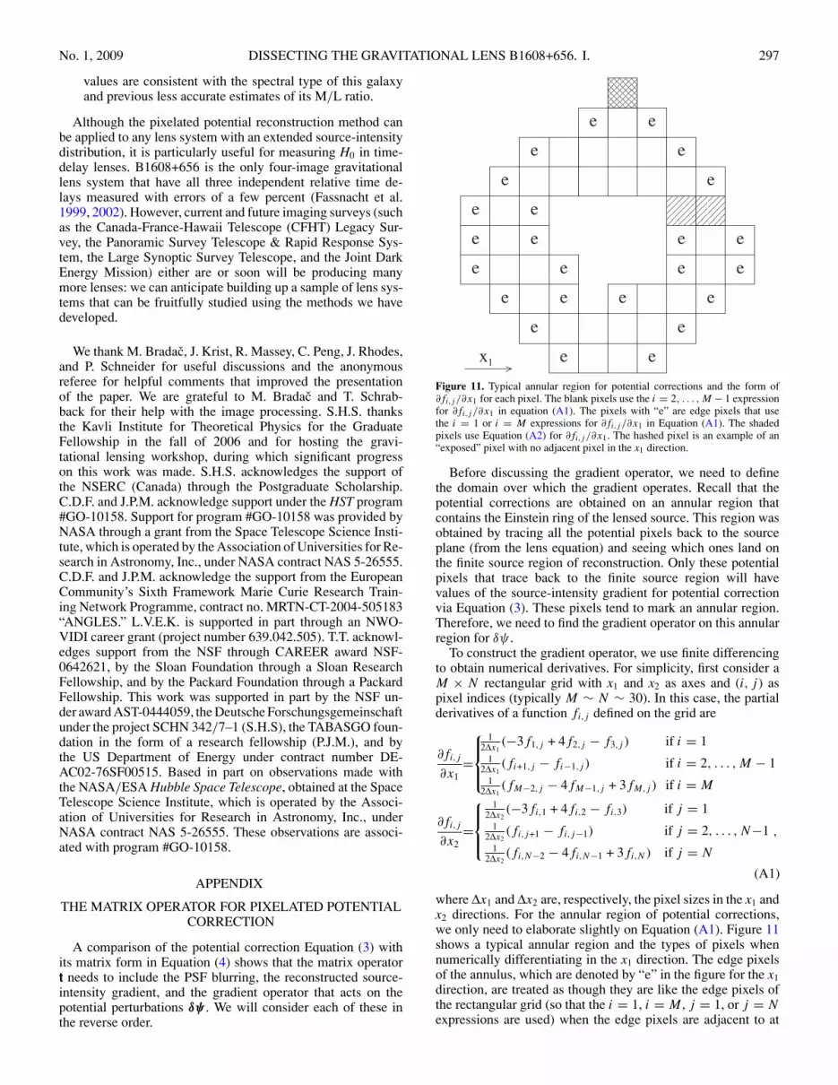
No. 1, 2009 DISSECTING THE GRAVITATIONAL LENS B1608+656. I. 297
values are consistent with the spectral type of this galaxyand previous less accurate estimates of its M/L ratio.
Although the pixelated potential reconstruction method canbe applied to any lens system with an extended source-intensitydistribution, it is particularly useful for measuring H0 in time-delay lenses. B1608+656 is the only four-image gravitationallens system that have all three independent relative time de-lays measured with errors of a few percent (Fassnacht et al.1999, 2002). However, current and future imaging surveys (suchas the Canada-France-Hawaii Telescope (CFHT) Legacy Sur-vey, the Panoramic Survey Telescope & Rapid Response Sys-tem, the Large Synoptic Survey Telescope, and the Joint DarkEnergy Mission) either are or soon will be producing manymore lenses: we can anticipate building up a sample of lens sys-tems that can be fruitfully studied using the methods we havedeveloped.
We thank M. Bradac, J. Krist, R. Massey, C. Peng, J. Rhodes,and P. Schneider for useful discussions and the anonymousreferee for helpful comments that improved the presentationof the paper. We are grateful to M. Bradac and T. Schrab-back for their help with the image processing. S.H.S. thanksthe Kavli Institute for Theoretical Physics for the GraduateFellowship in the fall of 2006 and for hosting the gravi-tational lensing workshop, during which significant progresson this work was made. S.H.S. acknowledges the support ofthe NSERC (Canada) through the Postgraduate Scholarship.C.D.F. and J.P.M. acknowledge support under the HST program#GO-10158. Support for program #GO-10158 was provided byNASA through a grant from the Space Telescope Science Insti-tute, which is operated by the Association of Universities for Re-search in Astronomy, Inc., under NASA contract NAS 5-26555.C.D.F. and J.P.M. acknowledge the support from the EuropeanCommunity’s Sixth Framework Marie Curie Research Train-ing Network Programme, contract no. MRTN-CT-2004-505183“ANGLES.” L.V.E.K. is supported in part through an NWO-VIDI career grant (project number 639.042.505). T.T. acknowl-edges support from the NSF through CAREER award NSF-0642621, by the Sloan Foundation through a Sloan ResearchFellowship, and by the Packard Foundation through a PackardFellowship. This work was supported in part by the NSF un-der award AST-0444059, the Deutsche Forschungsgemeinschaftunder the project SCHN 342/7–1 (S.H.S), the TABASGO foun-dation in the form of a research fellowship (P.J.M.), and bythe US Department of Energy under contract number DE-AC02-76SF00515. Based in part on observations made withthe NASA/ESA Hubble Space Telescope, obtained at the SpaceTelescope Science Institute, which is operated by the Associ-ation of Universities for Research in Astronomy, Inc., underNASA contract NAS 5-26555. These observations are associ-ated with program #GO-10158.
APPENDIX
THE MATRIX OPERATOR FOR PIXELATED POTENTIALCORRECTION
A comparison of the potential correction Equation (3) withits matrix form in Equation (4) shows that the matrix operatort needs to include the PSF blurring, the reconstructed source-intensity gradient, and the gradient operator that acts on thepotential perturbations δψ . We will consider each of these inthe reverse order.
1
e e
e
e
e
e
e e
e e
ee
ee
e
e e
e
e
e
ee
e
x
e
Figure 11. Typical annular region for potential corrections and the form of∂fi,j /∂x1 for each pixel. The blank pixels use the i = 2, . . . , M − 1 expressionfor ∂fi,j /∂x1 in equation (A1). The pixels with “e” are edge pixels that usethe i = 1 or i = M expressions for ∂fi,j /∂x1 in Equation (A1). The shadedpixels use Equation (A2) for ∂fi,j /∂x1. The hashed pixel is an example of an“exposed” pixel with no adjacent pixel in the x1 direction.
Before discussing the gradient operator, we need to definethe domain over which the gradient operates. Recall that thepotential corrections are obtained on an annular region thatcontains the Einstein ring of the lensed source. This region wasobtained by tracing all the potential pixels back to the sourceplane (from the lens equation) and seeing which ones land onthe finite source region of reconstruction. Only these potentialpixels that trace back to the finite source region will havevalues of the source-intensity gradient for potential correctionvia Equation (3). These pixels tend to mark an annular region.Therefore, we need to find the gradient operator on this annularregion for δψ .
To construct the gradient operator, we use finite differencingto obtain numerical derivatives. For simplicity, first consider aM × N rectangular grid with x1 and x2 as axes and (i, j ) aspixel indices (typically M ∼ N ∼ 30). In this case, the partialderivatives of a function fi,j defined on the grid are
∂fi,j
∂x1=
⎧⎪⎨⎪⎩
12Δx1
(−3f1,j + 4f2,j − f3,j ) if i = 11
2Δx1(fi+1,j − fi−1,j ) if i = 2, . . . , M − 1
12Δx1
(fM−2,j − 4fM−1,j + 3fM,j ) if i = M
∂fi,j
∂x2=
⎧⎪⎨⎪⎩
12Δx2
(−3fi,1 + 4fi,2 − fi,3) if j = 11
2Δx2(fi,j+1 − fi,j−1) if j = 2, . . . , N−1
12Δx2
(fi,N−2 − 4fi,N−1 + 3fi,N ) if j = N
,
(A1)
where Δx1 and Δx2 are, respectively, the pixel sizes in the x1 andx2 directions. For the annular region of potential corrections,we only need to elaborate slightly on Equation (A1). Figure 11shows a typical annular region and the types of pixels whennumerically differentiating in the x1 direction. The edge pixelsof the annulus, which are denoted by “e” in the figure for the x1direction, are treated as though they are like the edge pixels ofthe rectangular grid (so that the i = 1, i = M , j = 1, or j = Nexpressions are used) when the edge pixels are adjacent to at

298 SUYU ET AL. Vol. 691
least two other pixels in the annulus in the direction of whichthe numerical derivative is taken. If an edge pixel of the annulusis only adjacent to one other pixel in the direction of which thenumerical derivative is taken, such as the shaded pixels in thefigure for the x1 direction, then we construct the gradient bytaking the difference between the two and dividing by the pixelsize. For example, if fi,j is at the edge, and fi+1,j is also in theannulus (which will have to be an edge pixel if fi+2,j is not inthe annulus), then the numerical derivatives in the x1 directionfor both fi,j and fi+1,j are
∂fi,j
∂x1= fi+1,j − fi,j
Δx1. (A2)
A similar equation applies for the x2 direction. If an edge pixelin the annulus is “exposed” in the sense that in one of thedirections x1 or x2, it has no adjacent pixels in the annulus, thenthis pixel is removed from the annular region of reconstructionas no numerical derivative can be formed. An example of an“exposed” pixel in the x1 direction is the hashed pixel in thefigure. Following the above prescription, we can obtain thevalues (∂fi,j /∂x1, ∂fi,j /∂x2) of all the (i, j ) pixels in the annulusin terms of values of the function in the annulus fkl. Factoringout the fkl values, we obtain the gradient operator defined as twomatrices: D1 for ∂/∂x1 and D2 for ∂/∂x2.
To conform to the data grid (since the image residual andimage covariance matrix is defined on the data grid), we usebilinear interpolation. We overlay the data grid on the coarsergrid, and for every data pixel that lies inside the annular regionon the coarse grid, we bilinearly interpolate to get, effectively,gradient operators on the data grid. This gives us an Nd × Npmatrix G where each row (corresponding to a data pixel that lieswithin the annulus) has four nonzero values that correspond tothe coefficients of bilinearly interpolating among the four coarsepotential pixels surrounding this data pixel. Associated witheach data pixel are the source-intensity gradient values (∂I/∂β1and ∂I/∂β2) that were obtained by mapping the data pixel backto the source plane using the lens equation, and interpolating onthe reconstructed source-intensity gradient on the source grid.We define matrices G1 and G2 as the matrix G multiplied bythe source-intensity gradient components ∂I/∂β1 and ∂I/∂β2,respectively. By definition, G1 and G2 are also Nd×Np matrices.
Lastly, we represent the PSF as a blurring matrix (operator)B that is of dimensions Nd × Nd (see e.g., Section 4; Treu &Koopmans 2004). Note that this matrix B is different from thematrix in Section 2.2.1 that is the Hessian of the ED.
Combining all the pieces together, the matrix operator t is
t = B · G1 · D1 + B · G2 · D2, (A3)
which is of dimensions Nd × Np.For the gravitational lens system B1608+656, we also need
to include the effects of dust extinction, which we express asa diagonal matrix K. Tracing back along the light rays, weencounter the dust immediately after the PSF blurring (forthe light from the lensed source). Therefore, we include it inEquation (A3) after B to get the following expression for thematrix operator t that includes dust:
t = B · K · G1 · D1 + B · K · G2 · D2. (A4)
REFERENCES
Blandford, R., Surpi, G., & Kundic, T. 2001, in ASP Conf. Ser. 237, GravitationalLensing: Recent Progress and Future Goals, ed. T. G. Brainerd & C. S.Kochanek (San Francisco, CA: ASP), 65
Bradac, M., Schneider, P., Lombardi, M., & Erben, T. 2005, A&A,437, 39
Brewer, B. J., & Lewis, G. F. 2006, ApJ, 637, 608Cardelli, J. A., Clayton, G. C., & Mathis, J. S. 1989, ApJ, 345, 245Casertano, S., et al. 2000, AJ, 120, 2747Coleman, G. D., Wu, C.-C., & Weedman, D. W. 1980, ApJS, 43, 393Dressler, A., & Gunn, J. E. 1983, ApJ, 270, 7Dye, S., Evans, N. W., Belokurov, V., Warren, S. J., & Hewitt, P. 2008, MNRAS,
388, 384Dye, S., & Warren, S. J. 2005, ApJ, 623, 31Falco, E. E., Gorenstein, M. V., & Shapiro, I. I. 1985, ApJ, 289, L1Fassnacht, C. D., Gal, R. R., Lubin, L. M., McKean, J. P., Squires, G. K., &
Readhead, A. C. S. 2006, ApJ, 642, 30Fassnacht, C. D., Pearson, T. J., Readhead, A. C. S., Browne, I. W. A., Koopmans,
L. V. E., Myers, S. T., & Wilkinson, P. N. 1999, ApJ, 527, 498Fassnacht, C. D., Womble, D. S., Neugebauer, G., Browne, I. W. A., Readhead,
A. C. S., Matthews, K., & Pearson, T. J. 1996, ApJ, 460, L103Fassnacht, C. D., Xanthopoulos, E., Koopmans, L. V. E., & Rusin, D. 2002, ApJ,
581, 823Hollis, J. M., Dorband, J. E., & Yusef-Zadeh, F. 1992, ApJ, 386, 293Hu, W. 2005, in ASP Conf. Series 339, Observing Dark Energy, ed. S. C. Wolff
& T. R. Lauer (San Francisco, CA: ASP), 215Jee, M. J., et al. 2007, ApJ, 661, 728Jullo, E., Kneib, J.-P., Limousin, M., Elıasdottir, A., Marshall, P. J., & Verdugo,
T. 2007, New J. Phys., 9, 447Keeton, C. R. 2001, arXiv:astro-ph/0102340Kneib, J.-P., Ellis, R. S., Smail, I., Couch, W. J., & Sharples, R. M. 1996, ApJ,
471, 643Kochanek, C., Schneider, P., & Wambsganss, J. 2006, Gravitational Lensing:
Strong, Weak and Micro (New York: Springer)Kochanek, C. S. 1991, ApJ, 373, 354Koekemoer, A. M., Fruchter, A. S., Hook, R. N., & Hack, W. 2002, in Proc.
Workshop held at the Space Telescope Science Institute, The 2002 HSTCalibration Workshop: Hubble after the Installation of the ACS and theNICMOS Cooling System, ed. S. Arribas, A. Koekemoer, & B. Whitmore(Baltimore, MD: STScI), 337
Komatsu, E., et al. 2008, arXiv:0803.0547Koopmans, L. V. E. 2005, MNRAS, 363, 1136Koopmans, L. V. E., & Fassnacht, C. D. 1999, ApJ, 527, 513Koopmans, L. V. E., Treu, T., Fassnacht, C. D., Blandford, R. D., & Surpi, G.
2003, ApJ, 599, 70Kormann, R., Schneider, P., & Bartelmann, M. 1994, A&A, 284, 285Krist, J. E., & Hook, R. N. 1997, in The 1997 HST Calibration Workshop
with a New Generation of Instruments, ed. S. Casertano, R. Jedrzejewski,T. Keyes, & M. Stevens (Baltimore, MD: STScI), 192
MacKay, D. J. C. 1992, Neural Comput., 4, 415Marshall, P. 2006, MNRAS, 372, 1289Myers, S. T., et al. 1995, ApJ, 447, L5Pei, Y. C. 1992, ApJ, 395, 130Peng, C. Y., Ho, L. C., Impey, C. D., & Rix, H.-W. 2002, AJ, 124, 266Rhodes, J. D., et al. 2007, ApJS, 172, 203Saha, P., Coles, J., Maccio, A. V., & Williams, L. L. R. 2006, ApJ,
650, L17Sersic, J. L. 1968, Atlas de Galaxias Australes (Cordoba: Observatorio Astro-
nomico)Surpi, G., & Blandford, R. D. 2003, ApJ, 584, 100Suyu, S. H., & Blandford, R. D. 2006, MNRAS, 366, 39Suyu, S. H., Marshall, P. J., Hobson, M. P., & Blandford, R. D. 2006, MNRAS,
371, 983Treu, T., & Koopmans, L. V. E. 2004, ApJ, 611, 739van Dokkum, P. G., & Stanford, S. A. 2003, ApJ, 585, 78Vegetti, S., & Koopmans, L. V. E. 2008, arXiv:0805.0201Wallington, S., Kochanek, C. S., & Narayan, R. 1996, ApJ, 465, 64Warren, S. J., & Dye, S. 2003, ApJ, 590, 673Wayth, R. B., & Webster, R. L. 2006, MNRAS, 372, 1187Williams, L. L. R., & Saha, P. 2000, AJ, 119, 439York, T., Jackson, N., Browne, I. W. A., Wucknitz, O., & Skelton, J. E. 2005,
MNRAS, 357, 124


![[Dissecting aortic aneurysm simulating an acute myocardial infarct]](https://img.pdfslide.net/doc/110x75/63558f23922cbb7c550ca86c/dissecting-aortic-aneurysm-simulating-an-acute-myocardial-infarct.jpg)


